A habitat model for brown bear conservation and land use planning in the central Apennines

BIOLOGICAL

CONSERVATION

Biological Conservation 118 (2004) 141–150

www.elsevier.com/locate/biocon

A habitat model for brown bear conservation andland use planning in the central Apennines

Mario Posillico a,*, Alberto Meriggi b, Elisa Pagnin c, Sandro Lovari c, Luigi Russo d

a Gestione ex Azienda di Stato Foreste Demaniali, 67031 Castel di Sangro (AQ), Italyb Dipartimento di Biologia Animale, Universit�a di Pavia, 27100 Pavia, Italy

c Dipartimento di Scienze Ambientali, Sezione di Ecologia Comportamentale, Etologia e Gestione della Fauna, Universit�a di Siena, 53100 Siena, Italyd Parco Naturale Regionale Monti Simbruini, 00020 Jenne (RM), Italy

Received 23 November 2002; received in revised form 23 July 2003; accepted 29 July 2003

Abstract

We investigated the brown bear habitat suitability in an 8000 km2 study area encompassing Abruzzo, Latium, and Molise regions

in central-southern Italy. Based on long-term field surveys and published records, we classified bear habitat as occupied or unoc-

cupied in 92 out of 320 sample squares (5� 5 km). For each sample square 36 habitat variables were measured from topographic

maps and Corine land-cover III level digital maps. The influence of habitat features on bear presence was investigated by multi-

variate and one-way analyses of variance and by logistic regression analysis. The logistic model correctly classified 95.5% of sample

squares of bear presence and 93.8% of those where bears were absent. Average altitude, deciduous woodlands and ecotone length,

showed a positive relationship with bear presence, whereas vineyard-olive groves and shrublands were negatively correlated with

bear presence. No specific land management guidelines or strategies exist for bear conservation in central Italy, based on knowledge

of habitat–population relationships. The landscape scale habitat model we developed could be useful to predict bear occurrence, to

identify critical areas for a brown bear conservation strategy, and to enhance the arrangement of the protected areas network for the

conservation of this species.

� 2003 Elsevier Ltd. All rights reserved.

Keywords: Ursus arctos; Distribution; Habitat modelling; Management; Central Italy

1. Introduction

Worldwide, especially throughout densely populated

landscapes like those in central-southern Europe, hu-

man activities have often deprived wildlife of the mostsuitable habitat, confining large carnivores, e.g. bears, to

remote or less accessible areas (Swenson et al., 2000).

Once distributed along most of the Apennine mountain

chain, the brown bear (Ursus arctos) range in peninsular

Italy was gradually reduced because of habitat loss and

direct persecution (Febbo and Pellegrini, 1990). Today,

brown bears in central Italy exist as a remnant, isolated

* Corresponding author. Present address: Dipartimento di Scienze

Ambientali, Sezione di Ecologia Comportamentale, Etologia e Gesti-

one della Fauna, Universit�a di Siena, via P.A. Mattioli 4, 53100 Siena,

Italy. Tel.: +39-0577-23-2953/4; fax: +39-0577-23-2825.

E-mail address: [email protected] (M. Posillico).

0006-3207/$ - see front matter � 2003 Elsevier Ltd. All rights reserved.

doi:10.1016/j.biocon.2003.07.017

population inhabiting 3000–5000 km2 from Molise to

Marche and Umbria regions (Fig. 1). However, the most

densely and steadily occupied area is about 1500–2500

km2 wide, in the Apennine mountains of southern Ab-

ruzzo, Latium and Molise regions, surrounding theAbruzzo National Park (Meriggi et al., 2001). Minimum

bear population size, estimated by snow tracking in 1985

over 600 km2 (Abruzzo National Park+ 200 km2 of its

buffer area), was 38–39 bears (Boscagli, 1990). No

comprehensive estimates of population size have been

carried out, but a preliminary evaluation of average bear

density has been made by two DNA fingerprinting

studies through a part of the ‘‘core’’ distribution range.These suggest a population density of 1 bear/50–80 km2

(Lorenzini and Posillico, 2000; Forest Service, unpub-

lished data). At such densities, a small bear population

(e.g. 60 bears) might be distributed over a 3000–4800

km2 area. This fully protected, threatened bear

mail to: [email protected]

142 M. Posillico et al. / Biological Conservation 118 (2004) 141–150

population (Servheen, 1999) requires timely conserva-

tion strategies and a proactive management approach

(Peyton et al., 1999).

Active bear conservation is only scheduled within

protected areas and usually without common guidelines.Furthermore, no wide scale habitat management strat-

egies exist to accomplish bear conservation in central

Italy based on habitat–population relationships. The

available budget to conduct long-term research and time

are often limiting factors for bear conservation. Thus,

quantitative models could represent useful tools to as-

semble and synthesize existing knowledge to combine

research with conservation (Walters, 1986; Starfield,1997; Williams, 1997; Merrill et al., 1999; Gross and

Miller, 2001).

Our goal was to produce a model of bear–habitat

relationships to identify habitat variables (sensu Hall et

al., 1997) affecting bear presence at the home range level,

and to evaluate the effectiveness of the national and

regional networks of protected areas for bear conser-

vation. Brown bear occurrence through the eastern andnorthern parts of the former range is gradually in-

creasing in central Italy. Thus, our model could help to

predict the potential distribution of brown bears to

spread through their previous historical range, i.e. its

range during 16th–18th centuries, the earliest period for

which bear distribution is reasonably known (Febbo

and Pellegrini, 1990) and to identify critical areas for the

expansion of this population.

2. Methods

2.1. Study area

Our study area (8000 km2) was located in central

Italy, from Latium Apennines (west) to the Adriatic sea(east) (central coordinates: 41�510 North; 12�270 East)(Fig. 1). This area included the core bear range and

encompassed Latium, Abruzzo and Molise regions.

Land use was mainly deciduous forests (35%) and crops

(27%). Pastures (16%) and rocks (2%) were present

mainly on the ridges of the Apennine chain and olive-

tree groves, orchards and vineyards (4%) at the lowest

altitudes or along valley bottoms. Shrubland (11%)resulted mainly from re-colonisation of abandoned

pastures and cultivations and from forest degradation.

The climate ranges from Mediterranean type near the

sea coast to meso-Mediterranean and sub-Mediterra-

nean, with the increase of altitude. Urban areas and

villages (2%) were mainly located at low altitudes and

along valley bottoms. Lakes and rivers, wetlands and

perennial snowfields occupy the rest of the study area.These habitat features vary widely across the study

area, along north–south, east–west and altitudinal

gradients.

2.2. Habitat analysis

Using a Universal Transverse Mercator grid system

(UTM) we identified 320 sample squares of 25 km2 each

on a 5 km spaced grid. The size of the sample squareswas based on the average size of annual home ranges of

adult female brown bears. Because no data about home

range size of the Apennine bear population were avail-

able, we used data from Croatia where the estimated

female mean home range size was 107 km2 (SD ¼ 35.7;

range ¼ 78–147; N ¼ 3) (Huber and Roth, 1993). In

agreement with Laymon and Barrett (1986) and Schulz

and Joyce (1992), the sample square size we adopted wasroughly equal to 15–20% of the estimated home range.

For each sample square we measured 36 habitat vari-

ables of which 19 concerned land cover types, seven

landscape structure (McGarigal and Marks, 1995), five

human pressure, and five physical characteristics (Table

1). Percentage cover of each vegetation or landcover type

was measured from Corine land-cover III level vector

maps, issuedby theCentro Interregionale diCartografia –Ministry of the Environment. Corine land-covermaps are

based on a supervised, computer-aided classification of

Landsat Thematic Mapper imagery (pixel size

0.09 ha), providing a nationwide homogeneous landcover

database at a 1:100,000 scale. The interpretation

of Landsat imagery has been checked and enhanced us-

ing high resolution aerial images (1:70,000), allowing

a minimum mapping resolution finer than 6.3 ha (250�250m). Length of railways, sealed and unsealed roads and

trails were measured from vector data layers developed

from topographic maps (scale 1:100,000 and 1:25,000

respectively, Istituto Geografico Militare). We digitised

elevation contours and mapped elevation points (moun-

tain tops, springs, valley bottoms, etc.) from 1:25,000

topographic maps to build a digital terrain model (DTM)

in raster format. We calculated altitude variables (mean,maximum, minimum, range and standard deviation in m

a.s.l.) assigning an altitude value to a set of randompoints

(n ¼ 1000 per sample square) overlaid on the study area�sDTMand summarizing altitude values by sample square.

The Shannon–Wiener diversity index (HD)wasmeasured

as

HD ¼ �Xn

i¼1

ðPi � ln PiÞ;

where Pi is the proportion of the sample square occupied

by patch type i. All variables were measured by PatchAnalyst software (Elkie et al., 1999) and Spatial Analyst

(v. 2.0a) extension of Arcview� GIS (v. 3.2a, ESRI,

Redlands, CA, USA).

We determined the bear range within the study area

from literature and from data collected by several au-

thors (Russo, 1990; Boscagli et al., 1995; Posillico, 1996;

Posillico and Sammarone, 1997). Data on bear presence

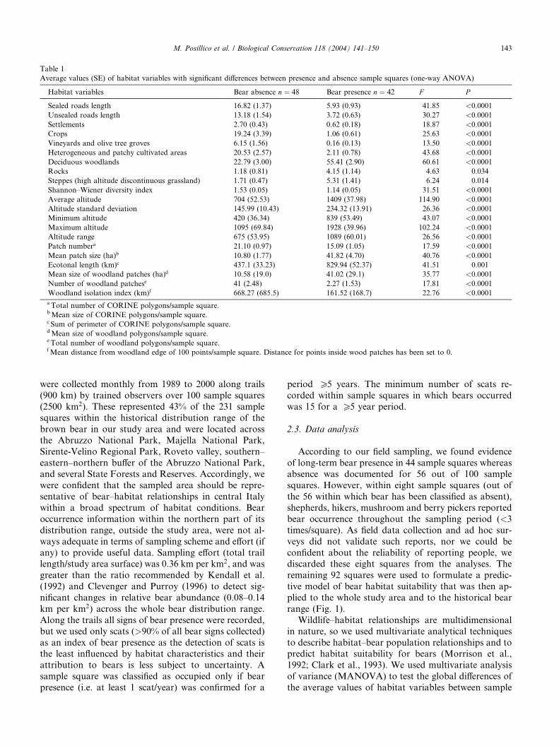
Table 1

Average values (SE) of habitat variables with significant differences between presence and absence sample squares (one-way ANOVA)

Habitat variables Bear absence n ¼ 48 Bear presence n ¼ 42 F P

Sealed roads length 16.82 (1.37) 5.93 (0.93) 41.85 <0.0001

Unsealed roads length 13.18 (1.54) 3.72 (0.63) 30.27 <0.0001

Settlements 2.70 (0.43) 0.62 (0.18) 18.87 <0.0001

Crops 19.24 (3.39) 1.06 (0.61) 25.63 <0.0001

Vineyards and olive tree groves 6.15 (1.56) 0.16 (0.13) 13.50 <0.0001

Heterogeneous and patchy cultivated areas 20.53 (2.57) 2.11 (0.78) 43.68 <0.0001

Deciduous woodlands 22.79 (3.00) 55.41 (2.90) 60.61 <0.0001

Rocks 1.18 (0.81) 4.15 (1.14) 4.63 0.034

Steppes (high altitude discontinuous grassland) 1.71 (0.47) 5.31 (1.41) 6.24 0.014

Shannon–Wiener diversity index 1.53 (0.05) 1.14 (0.05) 31.51 <0.0001

Average altitude 704 (52.53) 1409 (37.98) 114.90 <0.0001

Altitude standard deviation 145.99 (10.43) 234.32 (13.91) 26.36 <0.0001

Minimum altitude 420 (36.34) 839 (53.49) 43.07 <0.0001

Maximum altitude 1095 (69.84) 1928 (39.96) 102.24 <0.0001

Altitude range 675 (53.95) 1089 (60.01) 26.56 <0.0001

Patch numbera 21.10 (0.97) 15.09 (1.05) 17.59 <0.0001

Mean patch size (ha)b 10.80 (1.77) 41.82 (4.70) 40.76 <0.0001

Ecotonal length (km)c 437.1 (33.23) 829.94 (52.37) 41.51 0.001

Mean size of woodland patches (ha)d 10.58 (19.0) 41.02 (29.1) 35.77 <0.0001

Number of woodland patchese 41 (2.48) 2.27 (1.53) 17.81 <0.0001

Woodland isolation index (km)f 668.27 (685.5) 161.52 (168.7) 22.76 <0.0001

a Total number of CORINE polygons/sample square.bMean size of CORINE polygons/sample square.c Sum of perimeter of CORINE polygons/sample square.dMean size of woodland polygons/sample square.e Total number of woodland polygons/sample square.fMean distance from woodland edge of 100 points/sample square. Distance for points inside wood patches has been set to 0.

M. Posillico et al. / Biological Conservation 118 (2004) 141–150 143

were collected monthly from 1989 to 2000 along trails

(900 km) by trained observers over 100 sample squares

(2500 km2). These represented 43% of the 231 sample

squares within the historical distribution range of the

brown bear in our study area and were located across

the Abruzzo National Park, Majella National Park,

Sirente-Velino Regional Park, Roveto valley, southern–

eastern–northern buffer of the Abruzzo National Park,and several State Forests and Reserves. Accordingly, we

were confident that the sampled area should be repre-

sentative of bear–habitat relationships in central Italy

within a broad spectrum of habitat conditions. Bear

occurrence information within the northern part of its

distribution range, outside the study area, were not al-

ways adequate in terms of sampling scheme and effort (if

any) to provide useful data. Sampling effort (total traillength/study area surface) was 0.36 km per km2, and was

greater than the ratio recommended by Kendall et al.

(1992) and Clevenger and Purroy (1996) to detect sig-

nificant changes in relative bear abundance (0.08–0.14

km per km2) across the whole bear distribution range.

Along the trails all signs of bear presence were recorded,

but we used only scats (>90% of all bear signs collected)

as an index of bear presence as the detection of scats isthe least influenced by habitat characteristics and their

attribution to bears is less subject to uncertainty. A

sample square was classified as occupied only if bear

presence (i.e. at least 1 scat/year) was confirmed for a

period P5 years. The minimum number of scats re-

corded within sample squares in which bears occurred

was 15 for a P5 year period.

2.3. Data analysis

According to our field sampling, we found evidence

of long-term bear presence in 44 sample squares whereasabsence was documented for 56 out of 100 sample

squares. However, within eight sample squares (out of

the 56 within which bear has been classified as absent),

shepherds, hikers, mushroom and berry pickers reported

bear occurrence throughout the sampling period (<3

times/square). As field data collection and ad hoc sur-

veys did not validate such reports, nor we could be

confident about the reliability of reporting people, wediscarded these eight squares from the analyses. The

remaining 92 squares were used to formulate a predic-

tive model of bear habitat suitability that was then ap-

plied to the whole study area and to the historical bear

range (Fig. 1).

Wildlife–habitat relationships are multidimensional

in nature, so we used multivariate analytical techniques

to describe habitat–bear population relationships and topredict habitat suitability for bears (Morrison et al.,

1992; Clark et al., 1993). We used multivariate analysis

of variance (MANOVA) to test the global differences of

the average values of habitat variables between sample

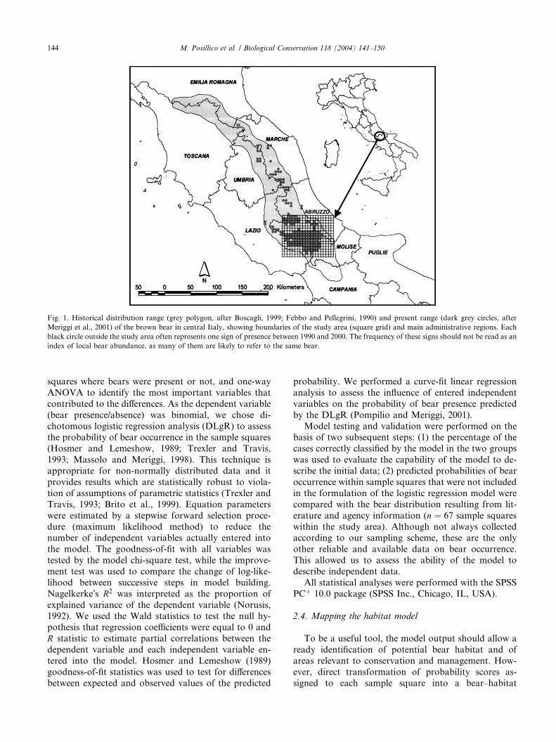
Fig. 1. Historical distribution range (grey polygon, after Boscagli, 1999; Febbo and Pellegrini, 1990) and present range (dark grey circles, after

Meriggi et al., 2001) of the brown bear in central Italy, showing boundaries of the study area (square grid) and main administrative regions. Each

black circle outside the study area often represents one sign of presence between 1990 and 2000. The frequency of these signs should not be read as an

index of local bear abundance, as many of them are likely to refer to the same bear.


squares where bears were present or not, and one-way

ANOVA to identify the most important variables that

contributed to the differences. As the dependent variable

(bear presence/absence) was binomial, we chose di-

chotomous logistic regression analysis (DLgR) to assessthe probability of bear occurrence in the sample squares

(Hosmer and Lemeshow, 1989; Trexler and Travis,

1993; Massolo and Meriggi, 1998). This technique is

appropriate for non-normally distributed data and it

provides results which are statistically robust to viola-

tion of assumptions of parametric statistics (Trexler and

Travis, 1993; Brito et al., 1999). Equation parameters

were estimated by a stepwise forward selection proce-dure (maximum likelihood method) to reduce the

number of independent variables actually entered into

the model. The goodness-of-fit with all variables was

tested by the model chi-square test, while the improve-

ment test was used to compare the change of log-like-

lihood between successive steps in model building.

Nagelkerke�s R2 was interpreted as the proportion of

explained variance of the dependent variable (Norusis,1992). We used the Wald statistics to test the null hy-

pothesis that regression coefficients were equal to 0 and

R statistic to estimate partial correlations between the

dependent variable and each independent variable en-

tered into the model. Hosmer and Lemeshow (1989)

goodness-of-fit statistics was used to test for differences

between expected and observed values of the predicted

probability. We performed a curve-fit linear regression

analysis to assess the influence of entered independent

variables on the probability of bear presence predicted

by the DLgR (Pompilio and Meriggi, 2001).

Model testing and validation were performed on thebasis of two subsequent steps: (1) the percentage of the

cases correctly classified by the model in the two groups

was used to evaluate the capability of the model to de-

scribe the initial data; (2) predicted probabilities of bear

occurrence within sample squares that were not included

in the formulation of the logistic regression model were

compared with the bear distribution resulting from lit-

erature and agency information (n ¼ 67 sample squareswithin the study area). Although not always collected

according to our sampling scheme, these are the only

other reliable and available data on bear occurrence.

This allowed us to assess the ability of the model to

describe independent data.

All statistical analyses were performed with the SPSS

PCþ 10.0 package (SPSS Inc., Chicago, IL, USA).

2.4. Mapping the habitat model

To be a useful tool, the model output should allow a

ready identification of potential bear habitat and of

areas relevant to conservation and management. How-

ever, direct transformation of probability scores as-

signed to each sample square into a bear–habitat


management map is unrealistic. First, the probability

score – and consequently management prescriptions –

assigned to every point within a sample square is influ-

enced by the position of the sampling grid used to

generate the model. The use of another – shifted – UTMsampling grid to calculate the probability of bear pres-

ence could produce different values for the same point,

with management options and priorities changing ac-

cordingly. Second, the model does not account for the

effect of adjacent probability scores on the value as-

signed to a given sample square or point. Thus, we built

15 additional sample square grids that were shifted 1.25

and 2.5 km east, west, north and south of the originalgrid. For the resulting 5120 sample squares (16 total

grids� 320 cells each) we ran a dichotomous logistic

regression model incorporating only the variables en-

tered in the original habitat model. The spatial inter-

section of the overlapping 16 grids produced 1.56 km2

pixels (1.25 km side), which was the mapping resolution

of our model. This is consistent with brown bear home

range size and with the spatial resolution of the Corinelandcover maps. The probability value assigned to each

pixel equalled the sum of the probability scores of the 16

overlapping squares divided by the number of overlap-

ping grids.

3. Results

We found significant broad differences between the

average values of habitat variables of squares with bear

presence and absence (Wilks� Lambda ¼ 0.2, d.f. ¼ 35,

P < 0:001). Twenty-one habitat variables significantly

contributed to these broad differences (Table 1). Vari-

ables related to human pressure were significantly lower

in the sample squares of bear presence, with the excep-

tion of railroad and trail length. Bear presence wassignificantly and positively associated with the extension

of deciduous woodlands and negatively associated to

woodland isolation index and woodland patch number

(Table 1). Crops, vineyard-olive groves, and heteroge-

neous cultivated areas showed average values signifi-

cantly lower in sample squares where bears were present.

The presence of the brown bear was significantly related

to rocks and steppe (i.e. high altitude discontinuous

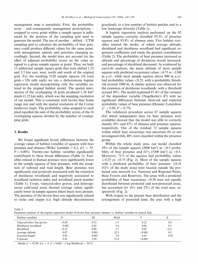
Table 2

Parameter estimate of the logistic regression model of brown bear presence–

Habitat variables B SE

Vineyard-olive tree groves )0.40 0.32

Deciduous woodland 0.042 0.02

Shrubland )0.22 0.09

Average altitude 0.07 0.001

Ecotonal length 0.03 0.001

Constant 9.81 2.50

Model v2 ¼ 97:99, d.f. ¼ 5, P < 0:001; )2 log likelihood ¼ 29.37.

grassland), to a low number of habitat patches and to a

low landscape diversity (Table 1).

A logistic regression analysis performed on the 92

sample squares correctly classified 95.5% of presence

squares and 93.8% of absence ones. Five habitat vari-ables entered the model, of which average altitude,

shrubland and deciduous woodland had significant re-

gression coefficients and made the greatest contribution

(Table 2). The probability of bear presence increased as

altitude and percentage of deciduous woods increased,

and percentage of shrubland decreased. As evidenced by

curve-fit analyses, the mean altitude of most sample

squares with predicted occurrence values >0.75 is >1100m a.s.l., while most sample squares above 900 m a.s.l.

had probability values <0.25, with a probability thresh-

old around 1000 m. A similar pattern was observed for

the extension of deciduous woodlands, with a threshold

around 50%. The model explained 87.4% of the variance

of the dependent variable (Nagelkerke�s R2) with no

significant differences between observed and expected

probability values of bear presence (Hosmer–Lemeshowv2 ¼ 5:08; P ¼ 0:75).

The validation procedure across 67 sample squares

(for which independent data on bear presence were

available) showed that the model was able to correctly

classify 93% and 87% of absence and presence squares,

respectively. Out of the residual 72 sample squares

within which bear occurrence was uncertain (8) or not

investigated (64), 40% were classified within the presencegroup.

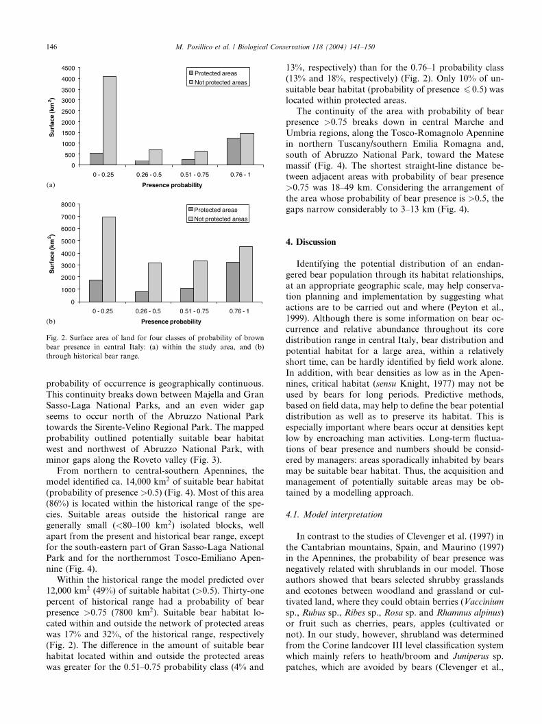
Within the whole study area, our model classified

39% of the sample squares (2800 km2) as >0.5 proba-

bility of bear presence and 61% (5200 km2) as <0.5.

Moreover, 71% of the squares had probability values

6 0.25 or >0.75 (Fig. 2). Most of the sample squares

with a predicted probability of bear presence 60.25

(52% of the study area) were located outside the pro-tected area network (i.e. National and Regional Parks,

State Forests and Reserves). The areas with a predicted

probability of bear occurrence >0.50 were not equally

distributed between protected and non-protected areas,

but accounted for 16% and 23% of the total area, re-

spectively (Fig. 2).

With respect to the present bear distribution and the

arrangement of protected land, the area with a high

absence vs. habitat variables in central Italy

Wald P R

1.5 0.22 0.0

3.4 0.06 0.1

5.7 0.02 )0.212.5 <0.001 0.3

3.8 0.05 0.01

15.4 <0.001

0

500

1000

1500

2000

2500

3000

3500

4000

4500

0 - 0.25 0.26 - 0.5 0.51 - 0.75 0.76 - 1

Presence probability

Su

rfac

e (k

m2 )

Protected areas

Not protected areas

0

1000

2000

3000

4000

5000

6000

7000

8000

0 - 0.25 0.26 - 0.5 0.51 - 0.75 0.76 - 1

Presence probability

Su

rfac

e (k

m2 )

Protected areas

Not protected areas

(a)

(b)

Fig. 2. Surface area of land for four classes of probability of brown

bear presence in central Italy: (a) within the study area, and (b)

through historical bear range.


probability of occurrence is geographically continuous.

This continuity breaks down between Majella and Gran

Sasso-Laga National Parks, and an even wider gap

seems to occur north of the Abruzzo National Park

towards the Sirente-Velino Regional Park. The mapped

probability outlined potentially suitable bear habitat

west and northwest of Abruzzo National Park, withminor gaps along the Roveto valley (Fig. 3).

From northern to central-southern Apennines, the

model identified ca. 14,000 km2 of suitable bear habitat

(probability of presence >0.5) (Fig. 4). Most of this area

(86%) is located within the historical range of the spe-

cies. Suitable areas outside the historical range are

generally small (<80–100 km2) isolated blocks, well

apart from the present and historical bear range, exceptfor the south-eastern part of Gran Sasso-Laga National

Park and for the northernmost Tosco-Emiliano Apen-

nine (Fig. 4).

Within the historical range the model predicted over

12,000 km2 (49%) of suitable habitat (>0.5). Thirty-one

percent of historical range had a probability of bear

presence >0.75 (7800 km2). Suitable bear habitat lo-

cated within and outside the network of protected areaswas 17% and 32%, of the historical range, respectively

(Fig. 2). The difference in the amount of suitable bear

habitat located within and outside the protected areas

was greater for the 0.51–0.75 probability class (4% and

13%, respectively) than for the 0.76–1 probability class

(13% and 18%, respectively) (Fig. 2). Only 10% of un-

suitable bear habitat (probability of presence 6 0.5) was

located within protected areas.

The continuity of the area with probability of bearpresence >0.75 breaks down in central Marche and

Umbria regions, along the Tosco-Romagnolo Apennine

in northern Tuscany/southern Emilia Romagna and,

south of Abruzzo National Park, toward the Matese

massif (Fig. 4). The shortest straight-line distance be-

tween adjacent areas with probability of bear presence

>0.75 was 18–49 km. Considering the arrangement of

the area whose probability of bear presence is >0.5, thegaps narrow considerably to 3–13 km (Fig. 4).

4. Discussion

Identifying the potential distribution of an endan-

gered bear population through its habitat relationships,

at an appropriate geographic scale, may help conserva-tion planning and implementation by suggesting what

actions are to be carried out and where (Peyton et al.,

1999). Although there is some information on bear oc-

currence and relative abundance throughout its core

distribution range in central Italy, bear distribution and

potential habitat for a large area, within a relatively

short time, can be hardly identified by field work alone.

In addition, with bear densities as low as in the Apen-nines, critical habitat (sensu Knight, 1977) may not be

used by bears for long periods. Predictive methods,

based on field data, may help to define the bear potential

distribution as well as to preserve its habitat. This is

especially important where bears occur at densities kept

low by encroaching man activities. Long-term fluctua-

tions of bear presence and numbers should be consid-

ered by managers: areas sporadically inhabited by bearsmay be suitable bear habitat. Thus, the acquisition and

management of potentially suitable areas may be ob-

tained by a modelling approach.

4.1. Model interpretation

In contrast to the studies of Clevenger et al. (1997) in

the Cantabrian mountains, Spain, and Maurino (1997)in the Apennines, the probability of bear presence was

negatively related with shrublands in our model. Those

authors showed that bears selected shrubby grasslands

and ecotones between woodland and grassland or cul-

tivated land, where they could obtain berries (Vaccinium

sp., Rubus sp., Ribes sp., Rosa sp. and Rhamnus alpinus)

or fruit such as cherries, pears, apples (cultivated or

not). In our study, however, shrubland was determinedfrom the Corine landcover III level classification system

which mainly refers to heath/broom and Juniperus sp.

patches, which are avoided by bears (Clevenger et al.,

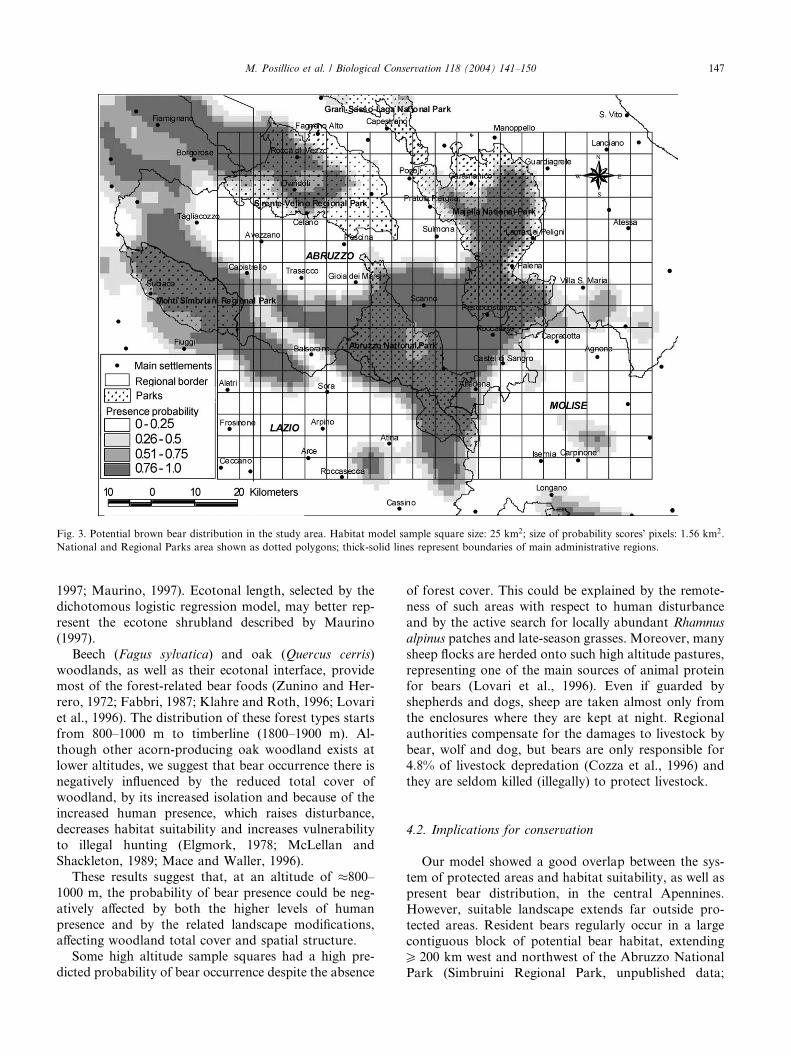
Fig. 3. Potential brown bear distribution in the study area. Habitat model sample square size: 25 km2; size of probability scores� pixels: 1.56 km2.

National and Regional Parks area shown as dotted polygons; thick-solid lines represent boundaries of main administrative regions.


1997; Maurino, 1997). Ecotonal length, selected by the

dichotomous logistic regression model, may better rep-

resent the ecotone shrubland described by Maurino

(1997).

Beech (Fagus sylvatica) and oak (Quercus cerris)

woodlands, as well as their ecotonal interface, providemost of the forest-related bear foods (Zunino and Her-

rero, 1972; Fabbri, 1987; Klahre and Roth, 1996; Lovari

et al., 1996). The distribution of these forest types starts

from 800–1000 m to timberline (1800–1900 m). Al-

though other acorn-producing oak woodland exists at

lower altitudes, we suggest that bear occurrence there is

negatively influenced by the reduced total cover of

woodland, by its increased isolation and because of theincreased human presence, which raises disturbance,

decreases habitat suitability and increases vulnerability

to illegal hunting (Elgmork, 1978; McLellan and

Shackleton, 1989; Mace and Waller, 1996).

These results suggest that, at an altitude of �800–

1000 m, the probability of bear presence could be neg-

atively affected by both the higher levels of human

presence and by the related landscape modifications,affecting woodland total cover and spatial structure.

Some high altitude sample squares had a high pre-

dicted probability of bear occurrence despite the absence

of forest cover. This could be explained by the remote-

ness of such areas with respect to human disturbance

and by the active search for locally abundant Rhamnus

alpinus patches and late-season grasses. Moreover, many

sheep flocks are herded onto such high altitude pastures,

representing one of the main sources of animal proteinfor bears (Lovari et al., 1996). Even if guarded by

shepherds and dogs, sheep are taken almost only from

the enclosures where they are kept at night. Regional

authorities compensate for the damages to livestock by

bear, wolf and dog, but bears are only responsible for

4.8% of livestock depredation (Cozza et al., 1996) and

they are seldom killed (illegally) to protect livestock.

4.2. Implications for conservation

Our model showed a good overlap between the sys-

tem of protected areas and habitat suitability, as well as

present bear distribution, in the central Apennines.

However, suitable landscape extends far outside pro-

tected areas. Resident bears regularly occur in a large

contiguous block of potential bear habitat, extendingP 200 km west and northwest of the Abruzzo National

Park (Simbruini Regional Park, unpublished data;

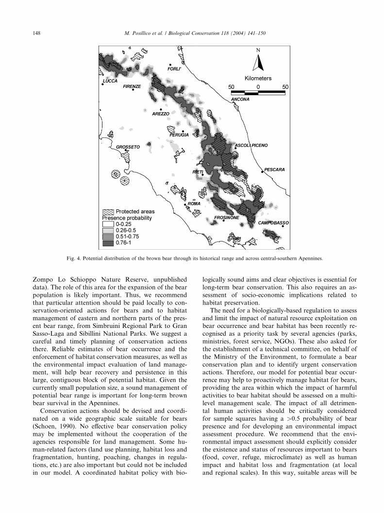
Fig. 4. Potential distribution of the brown bear through its historical range and across central-southern Apennines.


Zompo Lo Schioppo Nature Reserve, unpublished

data). The role of this area for the expansion of the bear

population is likely important. Thus, we recommend

that particular attention should be paid locally to con-

servation-oriented actions for bears and to habitatmanagement of eastern and northern parts of the pres-

ent bear range, from Simbruini Regional Park to Gran

Sasso-Laga and Sibillini National Parks. We suggest a

careful and timely planning of conservation actions

there. Reliable estimates of bear occurrence and the

enforcement of habitat conservation measures, as well as

the environmental impact evaluation of land manage-

ment, will help bear recovery and persistence in thislarge, contiguous block of potential habitat. Given the

currently small population size, a sound management of

potential bear range is important for long-term brown

bear survival in the Apennines.

Conservation actions should be devised and coordi-

nated on a wide geographic scale suitable for bears

(Schoen, 1990). No effective bear conservation policy

may be implemented without the cooperation of theagencies responsible for land management. Some hu-

man-related factors (land use planning, habitat loss and

fragmentation, hunting, poaching, changes in regula-

tions, etc.) are also important but could not be included

in our model. A coordinated habitat policy with bio-

logically sound aims and clear objectives is essential for

long-term bear conservation. This also requires an as-

sessment of socio-economic implications related to

habitat preservation.

The need for a biologically-based regulation to assessand limit the impact of natural resource exploitation on

bear occurrence and bear habitat has been recently re-

cognised as a priority task by several agencies (parks,

ministries, forest service, NGOs). These also asked for

the establishment of a technical committee, on behalf of

the Ministry of the Environment, to formulate a bear

conservation plan and to identify urgent conservation

actions. Therefore, our model for potential bear occur-rence may help to proactively manage habitat for bears,

providing the area within which the impact of harmful

activities to bear habitat should be assessed on a multi-

level management scale. The impact of all detrimen-

tal human activities should be critically considered

for sample squares having a >0.5 probability of bear

presence and for developing an environmental impact

assessment procedure. We recommend that the envi-ronmental impact assessment should explicitly consider

the existence and status of resources important to bears

(food, cover, refuge, microclimate) as well as human

impact and habitat loss and fragmentation (at local

and regional scales). In this way, suitable areas will be


preserved and population expansion and recovery of

bear could occur.

Acknowledgements

Our work has been endorsed and/or funded by the

Italian Ministry of the Environment (Nature Conser-

vation Direction) and by the Italian Ministry of Forests

and Agriculture (through a European Union grant,

LIFE99NAT/IT/006244). We thank P. Verucci, A. Ca-

rucci, B. Ragni, M. Spinetti and M. Dell�Orso for data

on recent bear presence within Latium, Umbria, Ab-ruzzo and Marche Regions. E. Dupr�e provided useful

suggestions as to GIS processing. A. Massolo provided

useful suggestions in statistics and habitat modelling.

We thank A. Cumer and I. Chiucchiarelli, who provided

Corine coverages and technical insight about Corine

landcover maps. We are particularly grateful to F. Van

Manen, N. Owen-Smith, F. Cassola and A. Clevenger

for revising our paper, their stimulating criticism as wellas for providing significant improvements.

References

Boscagli, G., 1990. Marsican brown bear population in Central Italy –

status report. Aquilo Series in Zoology 27, 81–83.

Boscagli, G., 1999. Status and management of the brown bear in

Central Italy (Abruzzo). In: Servheen, C., Herrero, S., Peyton, B.

(Eds.), Bears. Status Survey and Conservation Action Plan. IUCN/

SSC Bear and Polar Bear Specialist Group. IUCN, Gland

Switzerland, pp. 81–84.

Boscagli, G., Pellegrini, M., Febbo, D., Pellegrini, M., Cal�o, C.M.,

Castellucci, C., 1995. Distribuzione storica recente (1900–1991)

dell�orso bruno marsicano all�esterno del Parco Nazionale d�Ab-

ruzzo. Atti Societ�a Italiana di Scienze Naturali, Museo Civico di

Storia Naturale di Milano 134/1993, pp. 46–84.

Brito, J.C., Crespo, E.G., Paulo, O.S., 1999. Modelling wildlife

distributions: logistic multiple regression vs. overlap analysis.

Ecography 22, 251–260.

Clark, J.D., Dunn, J.E., Smith, K.G., 1993. A multivariate model of

black bear habitat use for a geographic information system.

Journal of Wildlife Management 57, 519–526.

Clevenger, A.P., Purroy, F.J., 1996. Sign surveys for estimating trend

of a remnant brown bear population in northern Spain. Wildlife

Biology 2, 275–281.

Clevenger, A.P., Purroy, F.J., Campos, M.A., 1997. Habitat assess-

ment of a relict brown bear population in Northern Spain.

Biological Conservation 80, 17–22.

Cozza, K., Fico, R., Battistini, M.L., Rogers, E., 1996. The damage–

conservation interface illustrated by predation on domestic live-

stock in central Italy. Biological Conservation 78, 329–336.

Elgmork, K., 1978. Human impact on a brown bear population.

Biological Conservation 13, 81–103.

Elkie, P.C., Rempel, R.S., Carr, A.P., 1999. Patch Analyst user�smanual. A tool for quantifying landscape structure. Northwest

Science & Technology, NWST Technical Manual TM-002. Ontario

Ministry for Natural Resources. Thunder Bay, Ontario, Canada.

Fabbri, M., 1987. Le abitudini alimentari dell�orso bruno nel Parco

Nazionale d�Abruzzo. M. Sc. (Laurea) Thesis, University of Parma,

Parma, Italy.

Febbo, D., Pellegrini, M., 1990. The historical presence of the

brown bear in the Apennines. Aquilo Series in Zoology 27,

85–88.

Gross, J.E., Miller, M.W., 2001. Chronic wasting disease in mule deer:

disease dynamics and control. Journal of Wildlife Management 65,

205–215.

Hall, L.S., Krausman, P.R., Morrison, M.L., 1997. The habitat

concept and a plea for standard terminology. Wildlife Society

Bulletin 25, 173–182.

Hosmer Jr., D.W., Lemeshow, S., 1989. Applied Logistic regression.

John Wiley and Sons, New York.

Huber, D., Roth, H.U., 1993. Movements of European brown bears in

Croatia. Acta Theriologica 38, 151–159.

Kendall, K.C., Metzgar, L.H., Patterson, D.A., Steele, B.M., 1992.

Power of sign surveys to monitor population trends. Ecological

Applications 2, 422–430.

Klahre, J., Roth, H.U., 1996. Nutritional preferences of Abruzzo

brown bears before hibernation. Abstracts. First Symposium of the

Italian Theriological Association, Perugia, October 1996.

Knight, R.R., 1977. Biological considerations in the delineation of

critical habitat. International Conference on Bear Research and

Management 3, 1–3.

Laymon, S.A., Barrett, R.H., 1986. Developing and testing habitat-

capability models: pitfalls and recommendations. In: Verner, J.,

Morrison, M.L., Ralph, C.J. (Eds.), Wildlife 2000. Modelling

Habitat Relationships of Terrestrial Vertebrates. University of

Wisconsin Press, Madison, WI, pp. 87–92.

Lorenzini, R., Posillico, M., 2000. DNA fingerprinting and brown bear

conservation in Abruzzo – central Italy. Italian Journal of Zoology

67, 326–327.

Lovari, S., Posillico, M., Varriale, M., Burrini, L., 1996. L�orso bruno

negli Altopiani maggiori d�Abruzzo. Final report to the Ministry of

Agriculture and Forests, Rome, Italy.

Mace, R.D., Waller, J.S., 1996. Grizzly bear distribution and human

conflicts in Jewel Basin Hiking Area, Swan Mountains, Montana.

Wildlife Society Bulletin 24, 461–467.

Massolo, A., Meriggi, A., 1998. Factors affecting habitat occupancy by

wolves in the northern Apennines (Northern Italy): a model of

habitat suitability. Ecography 21, 97–107.

Maurino, L., 1997. Uso dello habitat nell�orso bruno. M.Sc. (Laurea)

Thesis, University of Siena, Siena, Italy.

McGarigal, K., Marks B., 1995. FRAGSTATS: spatial pattern

analysis program for quantifying landscape structure. Gen Tech.

Rep. PNW-GTR-351. US Department of Agriculture, Forest

Service, Pacific Northwest Research Station, Portland, OR,

USA.

McLellan, B.N., Shackleton, D.M., 1989. Immediate reaction of

grizzly bears to human activities. Wildlife Society Bulletin 17, 269–

274.

Meriggi, A., Sacchi, O., Ziliani, U., Posillico, M., 2001. Definizione

dell�areale potenziale di cervo sardo, muflone e orso bruno. In:

Lovari, S. (Ed.), Progetto di monitoraggio dello stato di conserv-

azione di alcuni mammiferi particolarmente a rischio della fauna

italiana. Ministry of the Environment, Department for Nature

Conservation, Rome, Italy.

Merrill, T., Mattson, D.J., Wright, G.R., Quigley, H.B., 1999.

Defining landscapes suitable for the restoration of grizzly bears in

Idaho. Biological Conservation 87, 231–248.

Morrison, M.L., Marcot, G.B., Mannan, R.W., 1992. Wildlife–

Habitat Relationships: Concepts and Applications. University of

Wisconsin Press, Madison, WI.

Norusis M.J., 1992. SPSS/PC+ Advanced statistics, Ver. 5.0, Chicago.

Peyton, B., Servheen C., Herrero, S., 1999. An overview of bear

conservation planning and implementation. In: Servheen, C.,

Herrero, S., Peyton, B. (Eds.), Bears. Status Survey and Conser-

vation Action Plan. IUCN/SSC Bear and Polar Bear Specialist

Group, IUCN, Gland Switzerland, pp. 8–24.


Pompilio, L.,Meriggi, A., 2001.Modelling wild ungulate distribution in

Alpine habitat: a case study. Italian Journal of Zoology 68, 281–289.

Posillico, M., 1996. Brown bear presence in State Forests and

neighbour areas in Central Italy. Journal of Wildlife Research 1,

250–252.

Posillico, M., Sammarone, L., 1997. Relazione conclusiva del progetto

LIFE per la conservazione dell�orso bruno 1993–1997. Ministry of

Agriculture and Forests, State Forest Service, Rome, Italy.

Russo, L., 1990. L�orso bruno marsicano: dati preliminari dall�analisidelle schede faunistiche del Parco Nazionale d�Abruzzo. Bollettino

della Societ�a dei Naturalisti in Napoli 98–99, 107–122.

Servheen, C., 1999. Conservation of small bear populations through

strategic planning. Ursus 11, 67–74.

Schoen, J.W., 1990. Bear habitat management: a review and future

perspectives. International Conference on Bear Research and

Management 8, 143–154.

Schulz, T.T., Joyce, L.A., 1992. A spatial application of a marten

habitat model. Wildlife Society Bulletin 20, 74–83.

Starfield, A.M., 1997. A pragmatic approach to modelling for

wildlife management. Journal of Wildlife Management 61, 261–

270.

Swenson, J.E., Gerstl, N., Dahle, B., Zedrosser, A., 2000. Action Plan

for the Conservation of the Brown Bear in Europe. WWF

International, Gland, Switzerland.

Trexler, J.C., Travis, J., 1993. Non traditional regression analyses.

Ecology 74, 1629–1637.

Walters, C., 1986. Adaptive management of renewable resources.

Macmillan, New York.

Williams, B.K., 1997. Logic and science in wildlife biology. Journal of

Wildlife Management 61, 1007–1015.

Zunino, F., Herrero, S., 1972. The status of the brown bear in Abruzzo

National Park, 1971. Biological Conservation 4, 263–272.

A habitat model for brown bear conservation and land use planning in the central Apennines

Documents

Transcript of A habitat model for brown bear conservation and land use planning in the central Apennines