Konrad-Zuse-Zentrum fu r Informationstechnik Berlin

Takustraße 7 D-14195 Berlin-Dahlem

Germany

RALF KAHLER, MARK SIMON, HANS-CHRISTIAN HEGE

Fast Volume Rendering of Sparse Datasets Using Adaptive Mesh

Refinement

ZIB-Report 01-25 (July 2001)

Fast Volume Rendering of Sparse Datasets Using Adaptive Mesh Refinement

Ralf Kahler, Mark Simon, Hans-Christian Hege*

Abstract

In this paper we present an algorithm that accelerates 3D texture-based volume rendering of large and sparse data sets. A hierarchical data structure (known as AMR tree) consisting of nested uniform grids is employed in order to efficiently encode regions of interest. The hierarchies resulting from this kind of space partitioning yield a good balance between the amount of volume to render and the number of texture bricks – a prerequisite for fast rendering.

Comparing our approach to an octree based algorithm we show that our algorithm increases rendering performance significantly for sparse data. A further advantage is that less parameter tuning is necessary.

Keywords: scalar field visualization, volume rendering, 3D texture mapping, hierarchical space partitioning, AMR tree

1 Introduction 3D imaging and computational science produce increasingly large volumetric data sets. The number of voxels output by 3D imaging devices is proportional to the third power of their spatial resolution which continuously grows linear due to technical advances e.g. in detector technology. While data volumes consisting of O(109) voxels are not unusual today, future imaging devices and large scale simulations will create tera-scale data sets. These huge data sets have to be handled and explored interactively. Despite the enormous computer hardware development this remains a challenge.

Hierarchical representations allow to speed up the rendering process, typ­ically at the expense of some preprocessing time. Furthermore, they enable switching between different levels of detail, which greatly facilitates interactive navigation and provides appropriate means for data analysis of multiscale phe­nomena.

Since the early days of direct volume rendering, the prevalent types of ren­dering algorithms, namely ray casting [14, 19], cell projection, splatting [32], and volume rendering via 3D textures [9, 7, 34], have been accelerated by hier­archical volume representations.

Due to the advent of powerful texturing hardware, slice based volume ren­dering algorithms, either using 2D [11] or 3D texture mapping [7, 34], became

E-mail: {kaehler,mark.simon,hege}@zib.de .

1

very popular. They allow to obtain an image quality that suffices for many applications and make interactive frame rates on standard graphics hardware possible. The textures result from transfer functions that map the original data to color and opacity values. In case of 3D texture mapping, the texture coordi­nates at the polygon’s vertices are interpolated and determine a slice through the 3D texture. This approach leverages the trilinear interpolation hardware and has the additional advantage that textures need to be loaded only once, independent of the viewpoint. If the data set is too large to fit in texture mem­ory, the full volume may be rendered in multiple passes, placing only portions of the volume data, so called bricks, into the texture memory on each pass.

For sparse data sets the rendering speed can be significantly increased by skipping non-interesting regions, as noticed earlier in various volume rendering approaches. If the ratio of relevant to non-relevant volumes is small enough, this can be exploited with specialized variants of almost all types of volume rendering algorithms. This technique is well suited for interactive visualization, in particular if the criterion of relevance can be adjusted reasonable fast, such that user itself can ensure not to miss important details. More sophisticated approaches like truely error-controlled numerical computation of the volume ren­dering integrals, are more expensive and view-dependent. Furthermore, in many applications particular subvolumes shall be ignored deliberately, e.g. irrelevant spatial objects that have been identified in a preceding image segmentation step.

Disregarding irrelevant parts of the data volume is especially effective for spatially sparse data sets. Since such data occur frequently in nature i t is worthwhile to devise specific rendering algorithms. For instance in biomedical visualization, line-like structures, like vessel trees, neuron trees, trabeculae in bones, or filament structures in muscels, have to be visualized. Thin structures occur on all length scales in nature, ranging from chain molecules in chemistry to filaments of galaxies and galaxy clusters. In numerical simulations often large computational volumes have to be considered to take care of boundary condi­tions, though the interesting phenomena happen in very tight spatial regions. Here also a tight fitting of relevant subvolumes helps to save rendering time.

In case of rendering via 3D textures, sparsity of data can be exploited by assigning individual 3D textures – usually called texture bricks – to the relevant regions. The optimal coverage of the relevant subvolumes would be achieved by assigning a texture brick to each voxel that has been classified as relevant. This of course would result in an enormous number of texture and polygon coordi­nates to be computed and specified, since every brick has to be intersected with the proxy geometries (i.e. the slices to be rendered). Therefore a good balance between the volume enclosed by texture bricks and the number of created bricks is crucial.

In this paper we present an algorithm that achieves this balance by utilizing a hierarchical data structure, the so called adaptive mesh refinement (AMR) tree, which has been introduced by Marsha Berger in the 1980s for numerical gas dynamical simulations [5].

We compare the AMR-based algorithm with an octree-based algorithm and show that significant gains in rendering performance are achieved. The AMR-based algorithm has the additional advantage that i t requires less user inter­action for parameter adjustment, since its standard parameter settings already yield good rendering performance, almost independent of the topology and spa­tial distribution of the interesting subregions.

2

Section 2 surveys related work. We describe our approach in Section 3.1. In Section 3.2 we compare i t to an octree approach. Sections 4.1 and 4.2 address the 3D texture based rendering of AMR and octree hierarchies, respectively. In Section 5 we list performance results of the methods on different data sets. Conclusions and future work are presented in Sections 6 and 7, respectively.

2 Related Work

The idea to accelerate volume rendering algorithms by ignoring subregions that do not contribute to the final image has been pursued by many researchers. Levoy [20] presented a ray transversal algorithm that skips empty space by uti­lizing a hierarchical data structure indicating the presence of non-transparent material. The pyramidal data structure (a complete octree) has been employed by many researchers, too. Subramanian and Fussel [27] also designed a ray tracer that works efficiently when the data of interest is distributed sparsely through the volume. A simple preprocessing step identifies the voxels repre­senting features of interest and stores these in a kD-tree. The partitioned space is then efficiently ray-traced to render the voxel data.

Laur and Hanrahan [17] proposed a splatting algorithm that works on a pyramidal representation of the volume and chooses the number of splats adap-tively, according to user-supplied error criteria. Storing data mean and root mean square at each node permits rendering by progressive refinement. Nodes within the user-specified tolerance are rendered as single splats by utilizing tex­ture mapping capabilities.

Danskin and Hanrahan [10] presented algorithms that exploit homogeneity: not only empty, but also homogeneous regions are traversed in a fast manner. The algorithms enable to take into account also accumulated opacity. General­izing these ideas Wilhelms and Van Gelder used multi-dimensional trees, whose nodes contain also importance information which is used for selective traversal, e.g. in a coherent projection rendering approach [33].

Extending the idea of exploiting the distance transform to speed up the background traversal [35], Cohen and Sheffer [8] introduced so-called proxim­ity clouds that store the ’uniformity information’ typically encoded in a space partitioning tree directly in the voxel raster: voxel data contain either a data value or information indicating how far incident rays may leap without missing important features.

A different multiscale approach is to project the volume data into a wavelet basis and exploit this e.g. by performing the integration process for rays on the resulting wavelet coefficients directly [31]. This has been extended by Lippert and Gross [22], who employ Fourier descriptions of wavelet basis functions to efficiently compute line integrals.

Lee and Park [18] reduced ray-casting overheads by an adaptive block sub­division. Their algorithm applies a uniform space subdivision and then merges coherent uniform blocks in order to generate adaptive-sized blocks which are efficient for leaping space. They achieved 25% to 70% performance gain in rendering time over some octree implementation.

LaMar et. al. introduced a multiresolution technique for interactive texture-based volume visualization of very large data sets [16]. They also use an oc­tree representation and employ an adaptive scheme for rendering the volume in

3

regions-of-interest at high resolution and the volume away from these regions at progressively lower resolutions. Weiler et.al. [30] additionally developed meth­ods for avoiding artifacts that occur due to incorrect texture interpolation and opacity correction at brick boundaries. Boada et.al. [13] present an error and importance driven strategy for selecting a set of octree nodes from the full pyra­midal structure.

Some of these ideas have been extended for handling time-varying data sets. Ma et.al. [15] developed a corresponding octree encoding and rendering algo­rithm of time-varying volume data. Shen et. al. [25] proposed a data structure, called time-space partitioning (TSP) tree, that can effectively capture both the spatial and the temporal coherence from a time-varying field. This is utilized in a ray casting algorithm. In recent time this work has been extended to hardware volume rendering using 3D texture mapping [26].

For AMR data, resulting from simulations of hyperbolic PDEs by finite difference algorithms, a direct volume rendering using cell projection has been developed by Weber et.al. [29] and Ma [23].

Tong et.al. developed methods for volume block trimming and texture block merging in order to load only volume data hat contains important objects into texture memory [28]. Srinivasan et.al. [24] present an octree data structure to encapsulate non-transparent voxels.

We present an algorithm that in a first step creates an AMR hierarchy on base of the 3D image contents. I t utilizes a clustering algorithm for merging cells into rectilinear regions. In order to minimize waste of texture memory caused by OpenGL (and possibly hardware) restrictions as well as to reduce texture I/O, we employ a packing algorithm. The created hierarchies are rendered via hardware assisted 3D texture mapping.

3 Generating the Hierarchies

3.1 Generating the A M R Hierarchy

3.1.1 The A M R Data Structure

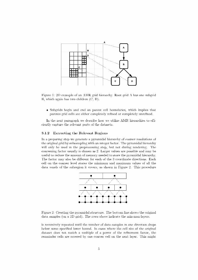
In the AMR approach the whole computational domain is covered by a coarse grid, representing the root node of the hierarchical data structure. In regions where higher resolution is required, finer subgrids are inserted as child nodes of the root grid. Together they define a new level of the hierarchy, increasing the resolution of their parent grid by a factor, usually referred to as refinement factor. Figure 1 shows a 2D example. This process repeats recursively until all grid cells on the finest resolution level satisfy certain error criteria, which depend on the particular numerical simulation. For simplification purposes the AMR schemes usually fulfill the following restrictions:

• The refinement factor is a positive integer, possibly different for the various spatial directions.

• The subgrids are axis-aligned, structured rectilinear meshes, consisting of hexahedral cells with constant edge lengths.

• Subgrids are completely contained within their parent grids.

4

B

C

Figure 1: 2D example of an AMR grid hierarchy. Root grid A has one subgrid B, which again has two children (C, D).

• Subgrids begin and end on parent cell boundaries, which implies that parents grid cells are either completely refined or completely unrefined.

In the next paragraph we describe how we utilize AMR hierarchies to effi­ciently capture the relevant parts of the datasets.

3.1.2 Extract ing the Relevant Regions

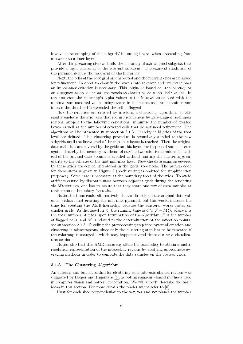
In a preparing step we generate a pyramidal hierarchy of coarser resolutions of the original grid by subsampling with an integer factor. The pyramidal hierarchy will only be used in the preprocessing step, but not during rendering. The coarsening factor usually is chosen as 2. Larger values are possible and may be useful to reduce the amount of memory needed to store the pyramidal hierarchy. The factor may also be different for each of the 3 coordinate directions. Each cell on the coarser level stores the minimum and maximum values of all the data voxels of the subregion i t covers, as shown in Figure 2. This procedure

* *

• • • •

111111111 Figure 2: Creating the pyramidal structure. The bottom line shows the original data samples (on a 2D grid). The rows above indicate the min-max-layers.

is recursively repeated until the number of data samples in one direction drops below some specified lower bound. In cases where the cell size of the original dataset does not match a multiple of a power of the refinement factor, the remainder cells are covered by one coarser cell on the next layer. This might

A

A

B

C D

5

involve some cropping of the subgrids’ bounding boxes, when descending from a coarser to a finer layer.

After this preparing step we build the hierarchy of axis-aligned subgrids that provide a tight enclosing of the relevant subareas. The coarsest resolution of the pyramid defines the root grid of the hierarchy.

Next, the cells of the root grid are inspected and the relevant ones are marked for refinement. In order to classify the voxels into relevant and irrelevant ones an importance criterion is necessary. This might be based on transparency or on a segmentation which assigns voxels to classes based upon their values. In the first case the colormap’s alpha values in the interval associated with the minimal and maximal values being stored in the coarse cells are examined and in case the threshold is exceeded the cell is flagged.

Now the subgrids are created by invoking a clustering algorithm. I t effi­ciently encloses the grid cells that require refinement by axis-aligned rectilinear regions, subject to the following conditions: minimize the number of created boxes as well as the number of covered cells that do not need refinement. The algorithm will be presented in subsection 3.1.3. Thereby child grids of the root level are defined. This clustering procedure is recursively applied to the new subgrids until the finest level of the min-max layers is reached. Then the original data cells that are covered by the grids on this layer, are inspected and clustered again. Thereby the memory overhead of storing two additional values for each cell of the original data volume is avoided without limiting the clustering gran­ularity to the cell size of the first min-max layer. Now the data samples covered by these grids are copied and stored in the grids’ tree node. The pseudo code for these steps is given in Figure 3 (re-clustering is omitted for simplification purposes). Some care is necessary at the boundary faces of the grids. To avoid artifacts caused by discontinuities between adjacent grids during the rendering via 3D-textures, one has to assure that they share one row of data samples at their common boundary faces [16].

Notice that one could alternatively cluster directly on the original data vol­ume, without first creating the min-max-pyramid, but this would increase the time for creating the AMR-hierarchy, because the clusterer works faster on smaller grids. As discussed in [6] the running time is O(k(P + M)) , where k is the total number of grids upon termination of the algorithm, P is the number of flagged cells, and M is related to the determination of the inflection points, see subsection 3.1.3. Dividing the preprocessing step into pyramid creation and clustering is advantageous, since only the clustering step has to be repeated if the colormap is changed – which may happen several times during a visualiza­tion session.

Notice also that this AMR hierarchy offers the possibility to obtain a multi­resolution representation of the interesting regions by applying appropriate av­eraging methods in order to compute the data samples on the coarser grids.

3.1.3 The Clustering Algor i thm

An efficient and fast algorithm for clustering cells into axis-aligned regions was suggested by Berger and Rigoutsos [6], adopting signature-based methods used in computer vision and pattern recognition. We will shortly describe the basic ideas in this section. For more details the reader might refer to [6].

First for each slice perpendicular to the x-y, x-z and y-z planes the number

6

struct AMRGrid { integer box[6]; pointer to data; pointer to children; pointer to parent;

}

AMRgrid createGrid(integer level, integer box[6])

{ generate subgrid;

if (level==maxlevel) { copy data samples to subgrid; insert subgrid into AMR_hierarchy;

} else { insert subgrid into AMR_hierarchy; markedCells=inspect(subgrid,

importance criterion); newBoxList=cluster(markedCells);

for each subbox in newBoxList { childGrid=createGrid(level+1, subbox); set subgrid as parent of childGrid; set childGrid as child of subgrid;

} } return subgrid;

}

create_hierarchy() { rootGrid = createGrid(0,rootLayerBox);

}

Figure 3: Pseudo code for creating the AMR hierarchy via clustering.

7

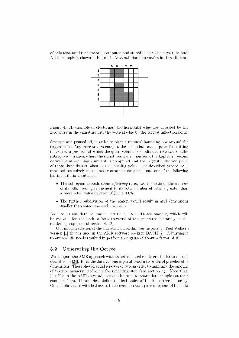
of cells that need refinement is computed and stored in so called signature lists. A 2D example is shown in Figure 4. Next exterior zero-entries in these lists are

5 6 6 2 2 3 3 0 2 3 5 5

Figure 4: 2D example of clustering: the horizontal edge was detected by the zero entry in the signature list, the vertical edge by the biggest inflection point.

detected and pruned off, in order to place a minimal bounding box around the flagged cells. Any interior zero entry in these lists indicates a potential cutting index, i.e. a position at which the given volume is subdivided into two smaller subregions. In cases where the signatures are all non-zero, the Laplacian second derivative of each signature list is computed and the biggest inflection point of these three lists is taken as the splitting point. The described procedure is repeated recursively on the newly created subregions, until one of the following halting criteria is satisfied:

• The subregion exceeds some efficiency ratio, i.e. the ratio of the number of its cells needing refinement to its total number of cells is greater than a preselected value between 0% and 100%.

• The further subdivision of the region would result in grid dimensions smaller than some minimal extension.

As a result the data volume is partitioned in a kD-tree manner, which will be relevant for the back-to-front traversal of the generated hierarchy in the rendering step (see subsection 4.1.2).

Our implementation of the clustering algorithm was inspired by Paul Walker’s version [1] that is used in the AMR software package DAGH [2]. Adjusting i t to our specific needs resulted in performance gains of about a factor of 10.

3.2 Generating the Octree

We compare the AMR approach with an octree based renderer, similar to the one described in [24]. First the data volume is partitioned into bricks of preselectable dimensions. These should equal a power of two, in order to minimize the amount of texture memory needed in the rendering step (see section 4). Note that, just like in the AMR case, adjacent nodes need to share data samples at their common faces. These bricks define the leaf nodes of the full octree hierarchy. Only subbranches with leaf nodes that cover non-transparent regions of the data

8

volume are inserted into the hierarchy. rendering performance is affected by

As mentioned in the introduction the

• the size of the subvolumes to render

the number of bricks. • the number of polygon and texture coordinates to be generated and thus

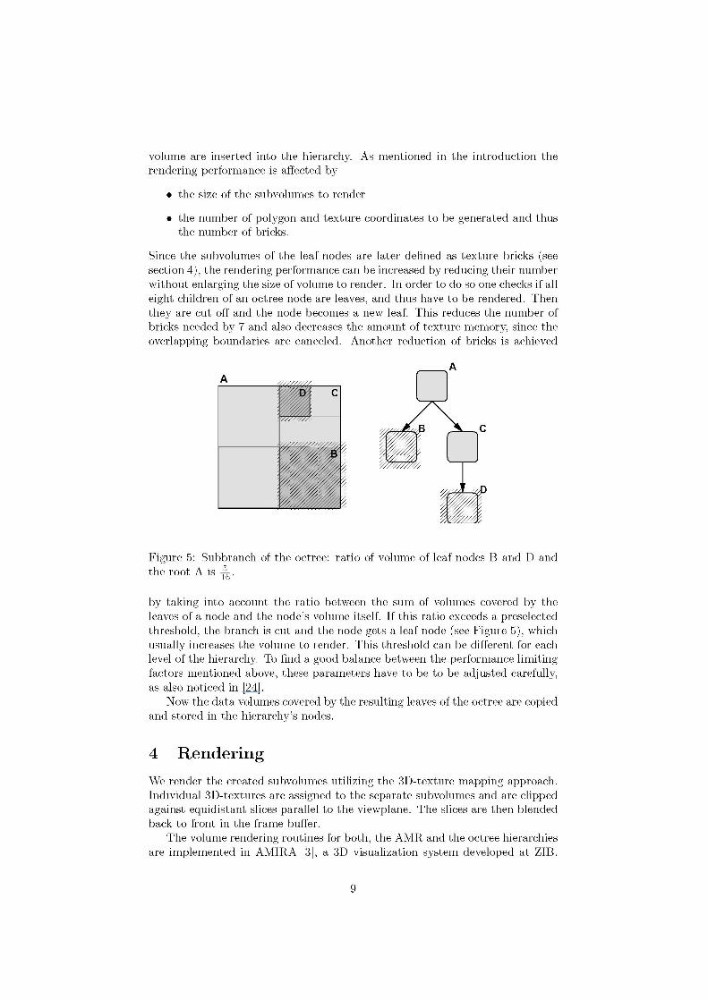
Since the subvolumes of the leaf nodes are later defined as texture bricks (see section 4), the rendering performance can be increased by reducing their number without enlarging the size of volume to render. In order to do so one checks if all eight children of an octree node are leaves, and thus have to be rendered. Then they are cut off and the node becomes a new leaf. This reduces the number of bricks needed by 7 and also decreases the amount of texture memory, since the overlapping boundaries are canceled. Another reduction of bricks is achieved

A A

(////////% B C

sssMssssD

Figure 5: Subbranch of the octree: ratio of volume of leaf nodes B and D and the root A is 1

56.

by taking into account the ratio between the sum of volumes covered by the leaves of a node and the node’s volume itself. If this ratio exceeds a preselected threshold, the branch is cut and the node gets a leaf node (see Figure 5), which usually increases the volume to render. This threshold can be different for each level of the hierarchy. To find a good balance between the performance limiting factors mentioned above, these parameters have to be to be adjusted carefully, as also noticed in [24].

Now the data volumes covered by the resulting leaves of the octree are copied and stored in the hierarchy’s nodes.

4 Rendering

We render the created subvolumes utilizing the 3D-texture mapping approach. Individual 3D-textures are assigned to the separate subvolumes and are clipped against equidistant slices parallel to the viewplane. The slices are then blended back-to-front in the frame buffer.

The volume rendering routines for both, the AMR and the octree hierarchies are implemented in AMIRA [3], a 3D visualization system developed at ZIB.

9

y 3max

8 8 9 10 y 2max

4 4 5 6 4 5 6 7 y 1max

1 2 3

X

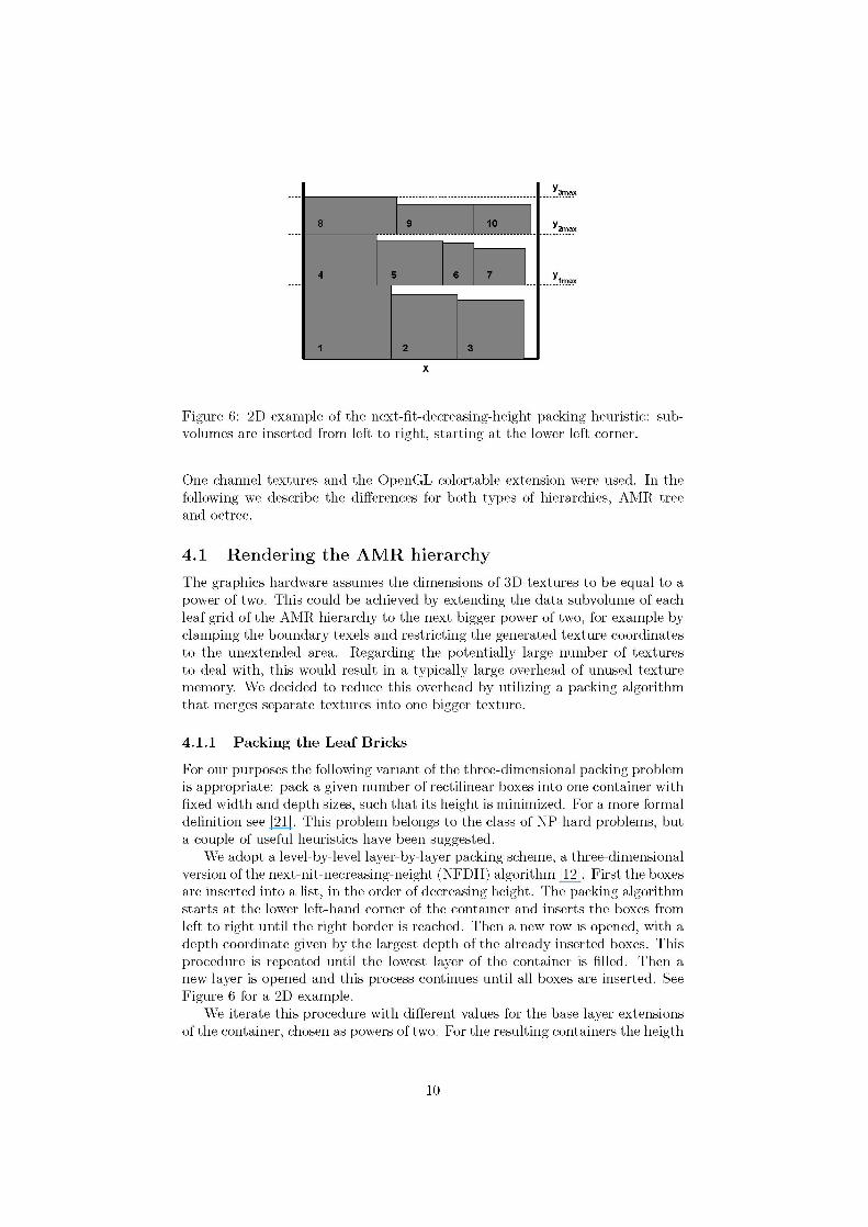
Figure 6: 2D example of the next-fit-decreasing-height packing heuristic: sub-volumes are inserted from left to right, starting at the lower left corner.

One channel textures and the OpenGL colortable extension were used. In the following we describe the differences for both types of hierarchies, AMR tree and octree.

4.1 Rendering the A M R hierarchy

The graphics hardware assumes the dimensions of 3D-textures to be equal to a power of two. This could be achieved by extending the data subvolume of each leaf grid of the AMR hierarchy to the next bigger power of two, for example by clamping the boundary texels and restricting the generated texture coordinates to the unextended area. Regarding the potentially large number of textures to deal with, this would result in a typically large overhead of unused texture memory. We decided to reduce this overhead by utilizing a packing algorithm that merges separate textures into one bigger texture.

4.1.1 Packing the Leaf Bricks

For our purposes the following variant of the three-dimensional packing problem is appropriate: pack a given number of rectilinear boxes into one container with fixed width and depth sizes, such that its height is minimized. For a more formal definition see [21]. This problem belongs to the class of NP-hard problems, but a couple of useful heuristics have been suggested.

We adopt a level-by-level layer-by-layer packing scheme, a three-dimensional version of the next-nit-necreasing-neight (NFDH) algorithm [12]. First the boxes are inserted into a list, in the order of decreasing height. The packing algorithm starts at the lower left-hand corner of the container and inserts the boxes from left to right until the right border is reached. Then a new row is opened, with a depth coordinate given by the largest depth of the already inserted boxes. This procedure is repeated until the lowest layer of the container is filled. Then a new layer is opened and this process continues until all boxes are inserted. See Figure 6 for a 2D example.

We iterate this procedure with different values for the base layer extensions of the container, chosen as powers of two. For the resulting containers the heigth

10

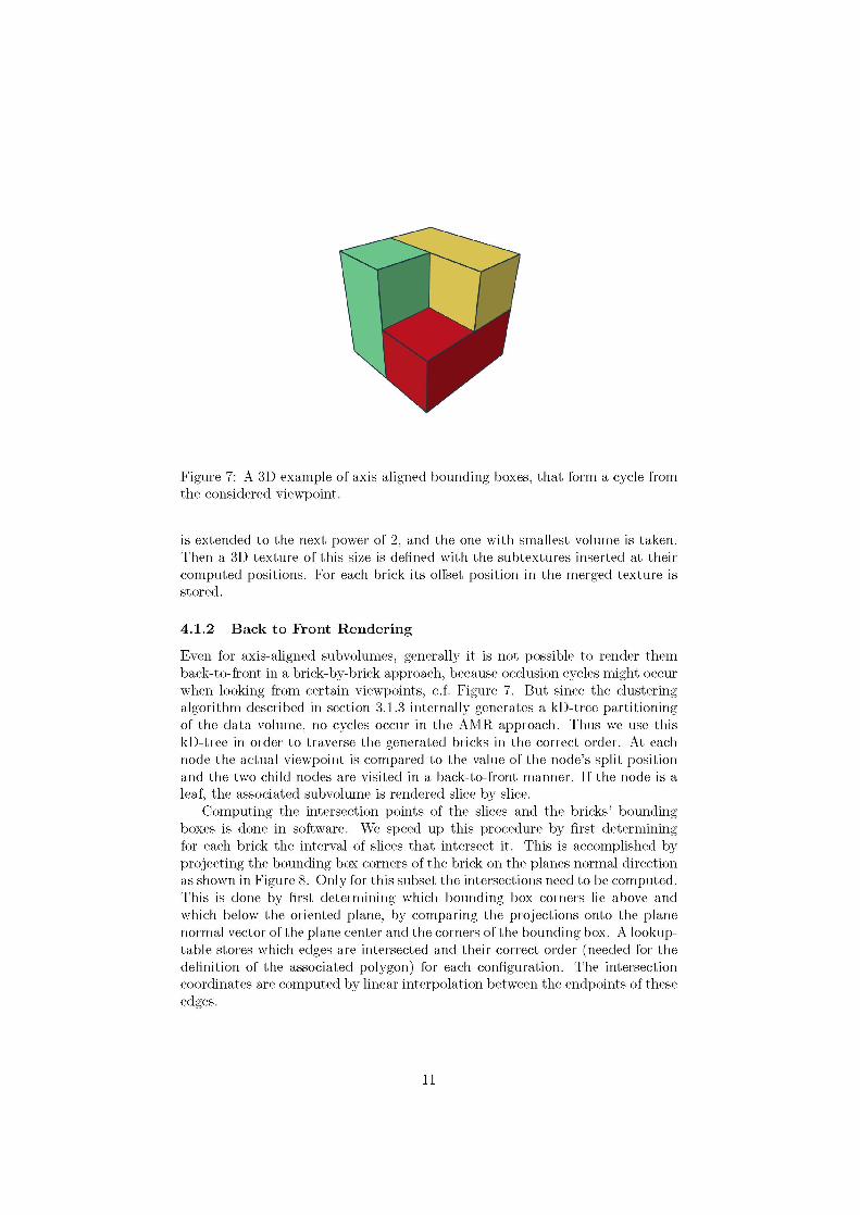
Figure 7: A 3D example of axis-aligned bounding boxes, that form a cycle from the considered viewpoint.

is extended to the next power of 2, and the one with smallest volume is taken. Then a 3D texture of this size is defined with the subtextures inserted at their computed positions. For each brick its offset position in the merged texture is stored.

4.1.2 Back to Front Rendering

Even for axis-aligned subvolumes, generally i t is not possible to render them back-to-front in a brick-by-brick approach, because occlusion cycles might occur when looking from certain viewpoints, c.f. Figure 7. But since the clustering algorithm described in section 3.1.3 internally generates a kD-tree partitioning of the data volume, no cycles occur in the AMR approach. Thus we use this kD-tree in order to traverse the generated bricks in the correct order. At each node the actual viewpoint is compared to the value of the node’s split position and the two child nodes are visited in a back-to-front manner. If the node is a leaf, the associated subvolume is rendered slice by slice.

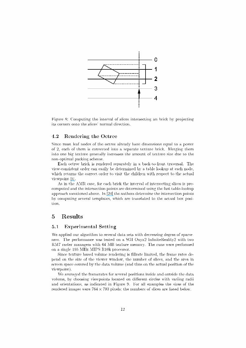
Computing the intersection points of the slices and the bricks’ bounding boxes is done in software. We speed up this procedure by first determining for each brick the interval of slices that intersect i t . This is accomplished by projecting the bounding box corners of the brick on the planes normal direction as shown in Figure 8. Only for this subset the intersections need to be computed. This is done by first determining which bounding box corners lie above and which below the oriented plane, by comparing the projections onto the plane normal vector of the plane center and the corners of the bounding box. A lookup-table stores which edges are intersected and their correct order (needed for the definition of the associated polygon) for each configuration. The intersection coordinates are computed by linear interpolation between the endpoints of these edges.

11

0

1

2

3

4 I Figure 8: Computing the interval of slices intersecting an brick by projecting its corners onto the slices’ normal direction.

4.2 Rendering the Octree

Since most leaf nodes of the octree already have dimensions equal to a power of 2, each of them is converted into a separate texture brick. Merging them into one big texture generally increases the amount of texture size due to the non-optimal packing scheme.

Each octree brick is rendered separately in a back-to-front traversal. The view-consistent order can easily be determined by a table lookup at each node, which returns the correct order to visit the children with respect to the actual viewpoint [4].

As in the AMR case, for each brick the interval of intersecting slices is pre-computed and the intersection points are determined using the fast table-lookup approach mentioned above. In [24] the authors determine the intersection points by computing several templates, which are translated to the actual box posi­tion.

5 Results

5.1 Experimental Setting

We applied our algorithm to several data sets with decreasing degree of sparse-ness. The performance was tested on a SGI Onyx2 InfiniteReality2 with two RM7 raster managers with 64 MB texture memory. The runs were performed on a single 195 MHz MIPS R10k processor.

Since texture based volume rendering is fillrate limited, the frame rates de­pend on the size of the viewer window, the number of slices, and the area in screen space covered by the data volume (and thus on the actual position of the viewpoint).

We averaged the framerates for several positions inside and outside the data volume, by choosing viewpoints located on different circles with variing radii and orientations, as indicated in Figure 9. For all examples the sizes of the rendered images were 764 × 793 pixels; the numbers of slices are listed below.

12

Figure 9: Some of the camera positions used for determination of the average rendering speed.

5.2 Input Data In the examples we used the opacity value as importance criterion. Voxels with an associated opacity value greater than α t h r e s = 0.03 were marked as relevant.

The datasets I and I I are confocal microscopy images of neurons inside a honey bee’s brain. About 0.1% respectively 0.2% voxels were marked as rele­vant and the volumes were rendered with 1.200 slices. For dataset I I a greater threshold of α t h r e s = 0.1 was used, in order to eliminate noise contained in the microscopy image.

Dataset I I I represents a part of a human vascular tree. Here 1.2% voxels were tagged as relevant. This dataset also was rendered with 1200 slices.

Example IV contains data from a molecular dynamics simulation and con-formational analysis. About 4% of voxels were marked as relevant. The volume was rendered with 320 slices. This is the only dataset which fitted into memory without bricking, i.e. in the standard volume rendering approach the frame rate was dominated by the fill rate.

The last example is a non sparse datatset containing 23% of relevant voxels, which was rendered with 900 slices.

Images of the different datasets are shown in Figure 10 to Figure 14. The left image of each figure shows an example volume rendering, the images in the middle depict the bounding boxes of the AMR hierarchy, and the right images display the octree bounding boxes.

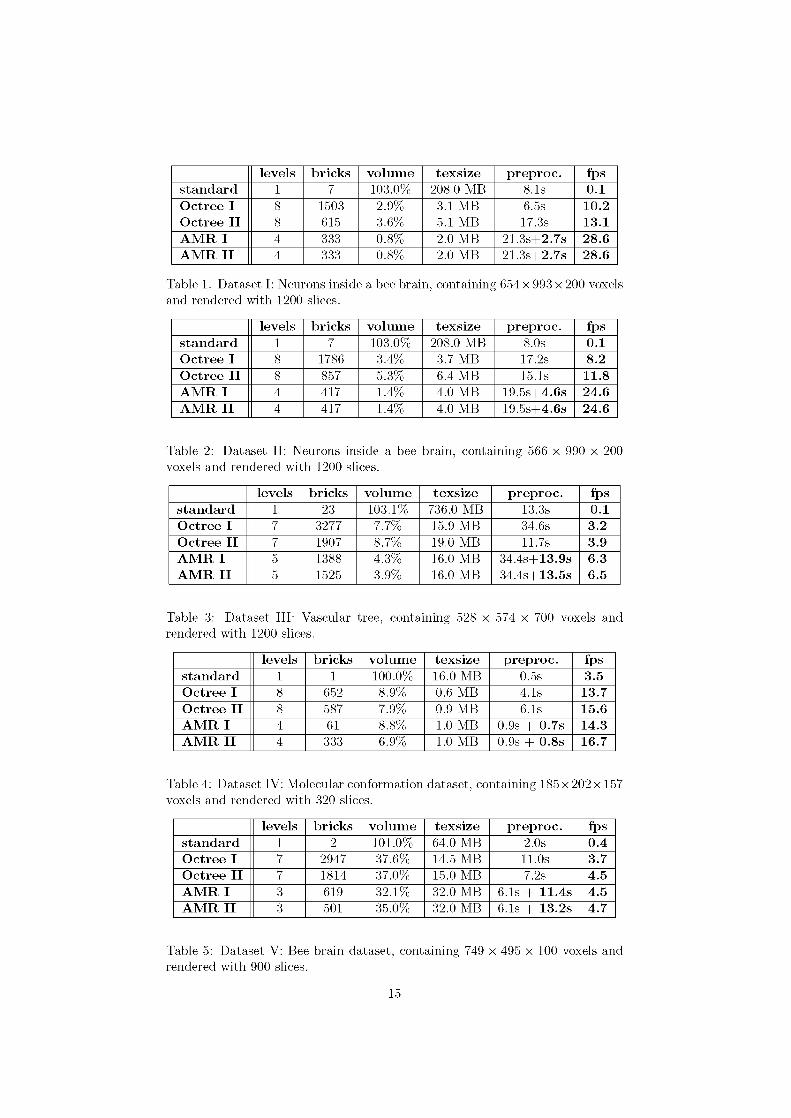
5.3 Experimental Results The statistics are shown in Tables 1 to 5. For each dataset we list the results for standard volume rendering, for the octree and the AMR approach. The first rows (‘Standard’) show the results for the standard volume rendering approach. Rows labeled ‘Octree I ’ contain the octree result with leaf dimensions that result in optimal frame rates. The ratio threshold was set to 1. Rows labeled ‘Octree

13

I I ’ show the best octree results we achieved, by adjusting the ratio threshold parameters. For the definition of these parameters see section 3.2.

The fourth rows (‘AMR I’) display AMR results with the clusterer’s effi­ciency parameter set to 0.85 and a minimal extension bound of 15. The last rows, labeled ‘AMR I I ’ , report the optimal results achieved by adjusting these parameters for each dataset. For datasets I and I I the entries for ‘AMR I ’ and ‘AMR I I ’ are identical because the parameters mentioned abouve already were optimal for these examples.

The tables’ columns list the number of created texture bricks, the percentage of the data volume covered by them, the amount of texture memory (after extension to the next power of 2 and packing them into one texture in the AMR case), the preprocessing times, the number of levels of the hierarchies and finally the frame rates. On the InfiniteReality2 the texelsize is 2, so the internal size of the textures is twice the number given in the table.

Note that for the datasets I,II,III and IV the volume entries for the standard case give values greater than 100%, because the bricks share a common row of voxels at their boundaries. For the standard approch the preprocessing times are just given by the times to allocate and define the texture or textures (in cases where bricking is necessary). The preprocessing times for the AMR hierarchies are split into the part needed for the resampling and a second part for clustering and packing. Note that only the clustering and packing step has to be updated, when the colormap is changed.

6 Conclusions

We presented an algorithm that accelerates the rendering of large datasets. The AMR approach achieves a good balance between the number of boxes needed for tightly capturing the relevant voxels of the data volume and the number of covered non-relevant ones. We compared our approach with the results of an octree based spatial subdivision. The number of created texture bricks is much smaller than the bricks created by the corresponding octree hierarchy, see Figures 1 to 5. Thus for the sparse datasets the AMR approach achieved significant performance gains. The frame rates for the standard and optimal parameter settings in the AMR cases are similar for all data sets. This shows that the standard setting usually yields good performance and hence almost no user interaction is necessary for finding optimal rendering parameters.

In contrast, the optimal parameter settings for the octree based algorithm vary strongly for the different datasets and are therefore difficult to determine for a given dataset.

We reduced the additional amount of texture memory caused by the power of 2 restrictions of OpenGL (respectively the graphics hardware), by packing several bricks into one bigger texture. For the datasets I, I I and I I I the best AMR results needed less texture memory compared to the best octree results. For dataset IV the size was almost equal. For the non-sparse dataset V the amount was twice as high as for the octree case.

So the AMR-based algorithm yields best results for sparse and large data sets and in this case has clear advantages compared to the octree-based one with regard to the frame rates, as well as to the amount of required texture memory.

14

levels bricks volume texsize preproc. fps standard 1 7 103.0% 208.0 MB 8.1s 0.1 Octree I 8 1503 2.9% 3.1 MB 6.5s 10.2 Octree I I 8 615 3.6% 5.1 MB 17.3s 13.1 A M R I 4 333 0.8% 2.0 MB 21.3s+2.7s 28.6 A M R I I 4 333 0.8% 2.0 MB 21.3s+2.7s 28.6

Table 1: Dataset I: Neurons inside a bee brain, containing 654×993×200 voxels and rendered with 1200 slices.

levels bricks volume texsize preproc. fps standard 1 7 103.0% 208.0 MB 8.0s 0.1 Octree I 8 1786 3.4% 3.7 MB 17.2s 8.2 Octree I I 8 857 5.3% 6.4 MB 15.1s 11.8 A M R I 4 417 1.4% 4.0 MB 19.5s+4.6s 24.6 A M R I I 4 417 1.4% 4.0 MB 19.5s+4.6s 24.6

Table 2: Dataset I I : Neurons inside a bee brain, containing 566 × 990 × 200 voxels and rendered with 1200 slices.

levels bricks volume texsize preproc. fps standard 1 23 103.1% 736.0 MB 13.3s 0.1 Octree I 7 3277 7.7% 15.9 MB 34.6s 3.2 Octree I I 7 1907 8.7% 19.0 MB 11.7s 3.9 A M R I 5 1388 4.3% 16.0 MB 34.4s+13.9s 6.3 A M R I I 5 1525 3.9% 16.0 MB 34.4s+13.5s 6.5

Table 3: Dataset I I I : Vascular tree, containing 528 × 574 × 700 voxels and rendered with 1200 slices.

levels bricks volume texsize preproc. fps standard 1 1 100.0% 16.0 MB 0.5s 3.5 Octree I 8 652 8.9% 0.6 MB 4.1s 13.7 Octree I I 8 587 7.9% 0.9 MB 6.1s 15.6 A M R I 4 61 8.8% 1.0 MB 0.9s + 0.7s 14.3 A M R I I 4 333 6.9% 1.0 MB 0.9s + 0.8s 16.7

Table 4: Dataset IV: Molecular conformation dataset, containing 185×202×157 voxels and rendered with 320 slices.

levels bricks volume texsize preproc. fps standard 1 2 101.0% 64.0 MB 2.0s 0.4 Octree I 7 2947 37.6% 14.5 MB 11.0s 3.7 Octree I I 7 1814 37.0% 15.0 MB 7.2s 4.5 A M R I 3 619 32.1% 32.0 MB 6.1s + 11.4s 4.5 A M R I I 3 501 35.0% 32.0 MB 6.1s + 13.2s 4.7

Table 5: Dataset V: Bee brain dataset, containing 749 × 495 × 100 voxels and rendered with 900 slices.

15

Even for the non-sparse data set V the AMR-based algorithm achieves frame rates comparable to those of the octree based algorithm.

7 Future Work

In order be forearmed for the large scale simulations and huge image data sets expected for the future we will optimize the texture packing approach. Fur­thermore we will examine the use of better packing algorithms, for example those similar to the one presented in [21]. I t would also be interesting to test other cluster algorithms and compare the preprocessing times and qualities of the resulting hierarchies.

Currently we are extending our algorithm for rendering data sets from AMR simulation, i.e. where an AMR hierarchy has already been established by the numerical solver. Here other requirements have to be considered, e.g. not refined areas have to be partitioned without introducing cycles. And one has to deal with the problem of opacity corrections and artifacts on the boundaries of grids with different levels of resolution.

8 Acknowledgments

We thank Malte Z¨ockler for the idea and implementation of the intersection al­gorithm based on a lookup-table, that was sketched in subsection 4.1.2 and Jo­hannes Schmidt-Ehrenberg, Detlev Stalling, Malte Z¨ockler and Werner Benger for proof reading and fruitful discussions respectively.

The single neuron and bee brain datasets where provided by Robert Brandt (research group Randolf Menzel, Freie Universit¨at Berlin), the vascular tree dataset by Thomas Lange (research group Peter Schlag, Robert-R¨ossle-Klinik and Unversit¨atsklinikum Charit´e, Berlin) and the molecular dataset by Jo­hannes Schmidt-Ehrenberg, Daniel Baum, and Frank Cordes (ZIB). This work was supported in part by the Max-Planck-Institut fu r Gravitation­sphysik (Albert-Einstein-Institut) in Potsdam/Germany.

References

[1] http://jean-luc.ncsa.uiuc.edu/Codes/3DCluster/.

[2] http://www.caip.rutgers.edu/ parashar/DAGH/.

[3] Amira User’s Guide and Reference Manual as well as Amira Programmer’s Guide. Konrad-Zuse-Zentrum fu r Informationstechnik Berlin (ZIB) and Indeed - Visual Concepts GmbH, Berlin, http://www.amiravis.com, 2000.

[4] Walid G. Aref and Hanan Samet. An algorithm for perspective viewing of objects represented by octrees. Computer Graphics Forum, 14(1):59–66, 1995.

[5] M. J. Berger and P. Collela. Local adaptive mesh refinement for shock hydrodynamics. J . Computational Physics, 82(1):64–84, 1989.

16

[6] Marsha Berger and Isidore Rigoutsos. An algorithm for point clustering and grid generation. IEEE Transactions on Systems, Man and Cybernetics, 21(5), 1991.

[7] B. Cabral, N. Cam, and J. Foran. Accelerated volume rendering and tomo-graphic reconstruction using texture mapping hardware. In Arie Kaufman and Wolfgang Krueger, editors, 1994 Symposium on Volume Visualization, pages 91–98, 1994.

[8] D. Cohen and Z. Sheffer. Proximity clouds: An acceleration technique for 3D grid traversal. The Visual Computer, 11:27–38, 1994.

[9] T. Cullip and U. Neumann. Accelerating volume reconstruction with 3D texture mapping hardware. Technical Report Technical Report TR93-027, Department of Computer Science at the University of North Carolina, Chapel Hill, 1993.

[10] John M. Danskin and Pat Hanrahan. Fast algorithms for volume ray trac­ing. In Workshop on Volume Visualization, pages 91–98, October 1992.

[11] Robert A. Drebin, Loren Carpenter, and Pat Hanrahan. Volume rendering. Computer Graphics (Proceedings of SIGGRAPH 88), 22(4):65–74, August 1988. Held in Atlanta, Georgia.

[12] D. S. Johnson E.G. Coffman, JR., M.R.Garey and R. E. Tarjan. Perfor­mance bounds for level-oriented two dimensional packing algorithms. SIAM Journal on Computing, 9:808–826, 1980.

[13] R.Scopigno I. Boada, I. Navazo. Multiresolution volume visualization with a texture-based octree. The Visual Computer, 17(5):185–197, 2001.

[14] James T. Kajiya and Brian P. Von Herzen. Ray tracing volume densities. Computer Graphics (Proceedings of SIGGRAPH 84), 18(3):165–174, July 1984. Held in Minneapolis, Minnesota.

[15] Kwan-Liu Ma, Diann Smith, Ming-Yun Shih and Han-Wei Shen. Efficient encoding and rendering of time-varying volume data. Technical report, ICASE Report No. 98-22 (NASA CR-1998-208424), Institute for Computer Applications in Science and Engineering, NASA Langley Research Center, Hampton, VA., June 1998.

[16] Eric C. LaMar, Bernd Hamann, and Kenneth I. Joy. Multiresolution tech­niques for interactive texture-based volume visualization. In David Ebert, Markus Gross, and Bernd Hamann, editors, IEEE Visualization ’99, pages 355–362, San Francisco, 1999. IEEE.

[17] David Laur and Pat Hanrahan. Hierarchical splatting: A progressive re­finement algorithm for volume rendering. Computer Graphics (Proceedings of SIGGRAPH 91), 25(4):285–288, July 1991. Held in Las Vegas, Nevada.

[18] Choong Hwan Lee and Kyo Ho Park. Fast volume rendering using adaptive block subdivision. Pacific Graphics ’97, October 1997. Held in Seoul, Korea.

17

[19] Marc Levoy. Display of surfaces from volume data. IEEE Computer Graph­ics & Applications, 8(3):29–37, May 1988.

[20] Marc Levoy. Efficient ray tracing of volume data. ACM Transactions on Graphics, 9(3):245–261, July 1990.

[21] Keqin Li and Kam-Hoi Cheng. On three-dimensional packing. SIAM Jour­nal on Computing, 19(5):847–867, 1990.

[22] L. Lippert and M. H. Gross. Fast wavelet based volume rendering by accumulation of transparent texture maps. Computer Graphics Forum, 14(3):431–444, 1995.

[23] Kwan-Liu Ma. Parallel rendering of 3d amr data on the sgi/cray t3e. Proc. 7th Symposium on Frontiers of Massively Parallel Computation, pages 138– 145, 1999.

[24] S. Huang R. Srinivasan, S. Fang. Rendering by template-based octree projection. Proceedings of the 8th Eurographics Workshop on Visualization in Scientific Computing, pages 155–163, 1997.

[25] Han-Wei Shen, Ling-Jan Chiang, and Kwan-Liu Ma. A fast volume render­ing algorithm for time-varying fields using a time-space partitioning (TSP) tree. In David Ebert, Markus Gross, and Bernd Hamann, editors, IEEE Visualization ’99, pages 371–378, San Francisco, 1999.

[26] Han-Wei Shen, David Ellsworth, and Ling-Jen Chiang. Accelerating time-varying hardware volume rendering using TSP trees and color-based error metrics. In Visualization and Graphics Symposium 2000, pages 119–128, Salt Lake City, UT, 2000.

[27] K. R. Subramanian and Donald S. Fussel. Applying space subdivision techniques to volume rendering. IEEE Visualization ’90, pages 150–159, 1990.

[28] X. Tong, W. Wang, W. Tsang, and Z. Tang. Efficiently rendering large volume data using texture mapping hardware. Joint EUROGRAPHICS - IEEE TCVG Symposium on Visualization, May 1999. Held in Vienna, Austria.

[29] Gunther H. Weber, Hans Hagen, Bernd Hamann, Kenneth I. Joy, Terry J. Ligocki, Kwan-Liu Ma, and John Shalf. Visualization of adaptive mesh refinement data. In Proceedings IS&T/SPIE Electronic Imaging 2001, 2001.

[30] M. Weiler, R. Westermann, C. Hansen, K. Zimmerman, and T. Ertl . Level-of-detail volume rendering via 3D textures. In IEEE Volume Visualization and Graphics Symposium 2000, pages 7–13, 1994.

[31] Ru¨diger Westermann. A multiresolution framework for volume rendering. 1994 Symposium on Volume Visualization, pages 51–58, October 1994.

[32] Lee Westover. Footprint evaluation for volume rendering. Computer Graph­ics (Proceedings of SIGGRAPH 90), 24(4):367–376, August 1990. ISBN 0-201-50933-4. Held in Dallas, Texas.

18

[33] Jane Wilhelms and Allen Van Gelder. Multi-dimensional trees for con­trolled volume rendering and compression. Technical Report UCSC-CRL-94-02, University of Santa Cruz, 1994.

[34] Orion Wilson, Allen VanGelder, and Jane Wilhelms. Direct volume ren­dering via 3D textures. Technical Report UCSC-CRL-94-19, University of Santa Cruz, 1994.

[35] K. Zuiderveld, A. Koning, and M. Viergever. Acceleration of ray-casting using 3d distance transforms. In Visualization in Biomedical Computing, Proceedings of VBC’92, pages 324–335. SPIE, 1992.

19

Figure 10: Dataset I, bee brain neuron, left: standard, middle: AMR, right: octree.

Figure 11: Dataset I I : bee brain neuron, left: standard, middle: AMR, right: octree.

Figure 12: Dataset I I I : vascular tree, left: standard, middle: AMR, right: oc­tree.

20

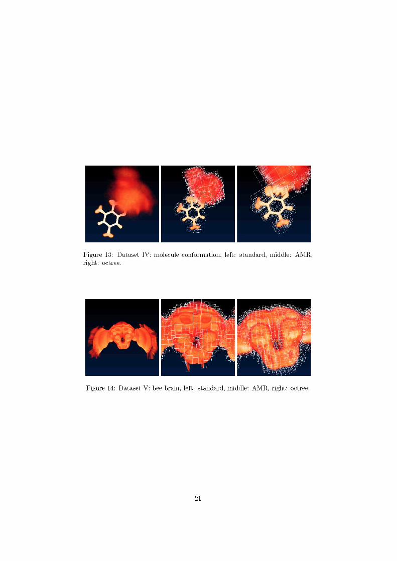
Figure 13: Dataset IV: molecule conformation, left: standard, middle: AMR, right: octree.

Figure 14: Dataset V: bee brain, left: standard, middle: AMR, right: octree.

21