AssessQueries for Interactive Analysis of Data CubesMatteo Francia

DISI - University of BolognaBologna, Italy

m.francia@unibo.it

Matteo GolfarelliDISI - University of Bologna

Bologna, Italymatteo.golfarelli@unibo.it

Patrick MarcelUniversity of Tours

Blois, Francepatrick.marcel@univ-tours.fr

Stefano RizziDISI - University of Bologna

Bologna, Italystefano.rizzi@unibo.it

Panos VassiliadisUniversity of Ioannina

Ioannina, Greecepvassil@cs.uoi.gr

ABSTRACTAssessment is the process of comparing the actual to the expectedbehavior of a business phenomenon and judging the outcome ofthe comparison. In this paper we propose assess, a novel query-ing operator that supports assessment based on the results of aquery on a data cube. This operator requires (1) the specificationof an OLAP query over a measure of a data cube, to define thetarget cube to be assessed; (2) the specification of a reference cubeof comparison (benchmark), which represents the expected per-formance of the measure; (3) the specification of how to performthe comparison between the target cube and the benchmark, and(4) a labeling function that classifies the result of this comparisonusing a set of labels. After introducing an SQL-like syntax forour operator, we formally define its semantics in terms of a setof logical operators. To support the computation of assess wepropose a basic plan as well as some optimization strategies, thenwe experimentally evaluate their performance using a prototype.

1 INTRODUCTIONAssume an analyst wants to assess the state of milk sales in Francefor 2019. She will have to issue a query against an OLAP server toobtain a cube, and then ask: “how good, normal, surprising, etc.is the situation I observe for this particular cube as compared tosome reference data?”. Assessment, as a process, is about compar-ing the actual to the expected behavior and judging, for instancethrough a labeling, the outcome of the comparison. Examples ofhow to assess the status of a cube (or of each single cell of a cube)include its comparison to:

(1) . . . a predefined target goal for the sales, e.g., because of theexistence of a predefined KPI (Key Performance Indicator);

(2) . . . a predefined golden standard, acting as a referencebenchmark (e.g., comparing French milk sales against theEU average) or, as an example in another domain, compar-ing a stock value to the S&P 500 index);

(3) . . . sibling cells, i.e., cells describing a similar context andsharing some dimension values (i.e., compare sales foryogurt and ice-cream in Greece in 2019, or milk sales inSpain and Italy for 2019);

(4) . . . the expected status of the cube as can be predicted fromthe past (e.g., compare actual milk sales in December 2018with those that can be predicted from the sales of theprevious six months).

© 2021 Copyright held by the owner/author(s). Published in Proceedings of the24th International Conference on Extending Database Technology (EDBT), March23-26, 2021, ISBN 978-3-89318-084-4 on OpenProceedings.org.Distribution of this paper is permitted under the terms of the Creative Commonslicense CC-by-nc-nd 4.0.

(5) . . . a new, derived measure produced via a function whoseformula involves other measures (e.g., profit=storeSales-storeCost).

This kind of tabular data assessment is consistently reportedas a frequent activity of data explorers [3, 12, 23] who often useSQL in combination with languages like Python and R. Notice-ably, assessment is one of the user’s intentions considered in theIntentional Analytics Model (IAM), which has been envisionedas a way to tightly couple OLAP and analytics [4, 21]. The IAMapproach relies on two major cornerstones: (i) the user exploresthe data space by expressing her analysis intentions rather thanby explicitly stating what data she needs, and (ii) in return shereceives both multidimensional data and knowledge insights inthe form of annotations of interesting subsets of data. Amongthe five intention operators proposed, assess is meant to judge acube measure with reference to some baseline.

In this paper we adopt the OLAP-centered nature of the IAMand operate in the context of a traditional OLAP environmentwith cubes, dimensions, hierarchies, and measures. This allowsus to take advantage of the neat logical-level schema structure ofOLAP and focus on the essence of the paper, which is proposingan assess operator to complement the traditional OLAP roll-up’sand drill-down’s. The idea of how to perform an assessment forthe measure values of a cube encompasses (a) the specificationof another cube, called benchmark, that represents the expectedor desirable performance of the measure; (b) the comparisonof the measure under investigation to the benchmark measure(for instance via a simple mathematical difference); and (c) thecharacterization, or labeling, of the status of the original cellbased on the result of the comparison.

Example 1.1. Given a SALES cube, the user’s intention de-scribed above can be expressed with this statement:

with SALES

for year = ’2019’, product = ’milk’by year, product

assess quantity against 1000

using ratio(quantity, 1000)

labels {[0, 0.9): bad, [0.9, 1.1]: acceptable, (1.1,inf): good}

Intuitively, the total quantity of milk sold in France in 2019 islabeled as bad/acceptable/good depending on the ratio with thetarget value 1000. □

Summary of contributions. Our contributions can be listedas follows:

• We introduce a novel operator, assess, that allows to au-tomatically evaluate and characterize the result of a cubequery.

Series ISSN: 2367-2005 121 10.5441/002/edbt.2021.12

• We introduce alternatives for specifying benchmarks, com-parison, and labeling schemes against which the resultsof a cube query can be compared and evaluated. For eachalternative we provide rigorous definitions and semantics,based on a set of logical operators, as well an SQL-likesyntax for the specification of an assess statement.

• We discuss alternative plans for the execution of assessstatements and experimentally evaluate them for theirefficiency and scalability.

Roadmap. In Section 2 we formalize the involved conceptsand give definitions. In Section 3 we explain how assessmentsare computed and introduce the alternatives of the assess opera-tor, while in Section 4 we provide its syntax and semantics. InSection 5 we present alternative strategies for query executionand in Section 6 we experimentally evaluate them. In Section 7we discuss the related work. Finally, in Section 8 we summarizeour findings and discuss our future work.

2 FORMALITIESTo simplify the formalization, we will restrict to consider linearhierarchies.

Definition 2.1 (Hierarchy and Cube Schema). A hierarchy is atriple ℎ = (𝐿, ⪰, ≥) where:(i) 𝐿 is a set of categorical levels, each coupled with a domain

of values (a.k.a. as members), 𝐷𝑜𝑚(𝑙) ;(ii) ⪰ is a roll-up total order of 𝐿; and(iii) ≥ is a part-of partial order of

⋃𝑙 ∈𝐿 𝐷𝑜𝑚(𝑙).

The part-of partial order is such that, for each couple of levels𝑙 and 𝑙 ′ such that 𝑙 ⪰ 𝑙 ′, for each member 𝑢 ∈ 𝐷𝑜𝑚(𝑙) there isexactly one member 𝑢 ′ ∈ 𝐷𝑜𝑚(𝑙 ′) such that 𝑢 ≥ 𝑢 ′.

A cube schema is a couple C = (𝐻,𝑀) where:(i) 𝐻 is a set of hierarchies;(ii) 𝑀 is a tuple1 of numerical measures, each coupled with one

aggregation operator 𝑜𝑝 (𝑚) ∈ {sum, avg, . . .}.

Example 2.2. As a working example we will use cube schemaSALES = (𝐻,𝑀), where

𝐻 = {ℎDate, ℎCustomer, ℎProduct, ℎStore},𝑀 = ⟨quantity, storeSales, storeCost⟩,date ⪰ month ⪰ year,

customer ⪰ gender,

product ⪰ type ⪰ category,

store ⪰ city ⪰ country

and 𝑜𝑝 (quantity) = 𝑜𝑝 (storeSales) = 𝑜𝑝 (storeCost) = sum. Asto the part-of partial order we have, for instance, Fresh Fruit ≥Fruit and 1997-04-15 ≥ 1997. □

Aggregation is the basic mechanism to query cubes, and itis captured by the following definition of group-by set. As nor-mally done when working with the multidimensional model, ifa hierarchy ℎ does not appear in a group-by set it is implicitlyassumed that a complete aggregation is done along ℎ.

Definition 2.3 (Group-by Set and Coordinate). Given cube schemaC = (𝐻,𝑀), a group-by set of C is a tuple of levels, at most onefrom each hierarchy of 𝐻 . The partial order induced on the setof all group-by sets of C by the roll-up orders of the hierarchies1When dealing with tuples we will write 𝑡1 = 𝑡2 |𝑠𝑜𝑟𝑡 (𝑡1 )

to denote that tuple 𝑡1 iscontained in tuple 𝑡2; (𝑡1, 𝑡2) to denote the tuple that concatenates 𝑡1 and 𝑡2; 𝑡 |𝑋to denote the projection of tuple 𝑡 on its component(s) 𝑋 [1].

in 𝐻 , is denoted with ⪰𝐻 . A coordinate of group-by set 𝐺 is atuple of members, one for each level of 𝐺 . Given coordinate 𝛾 ofgroup-by set 𝐺 and another group-by set 𝐺 ′ such that 𝐺 ⪰𝐻 𝐺 ′,we will denote with 𝑟𝑢𝑝𝐺′ (𝛾) the coordinate of 𝐺 ′ whose mem-bers are related to the corresponding members of 𝛾 in the part-oforders, and we will say that 𝛾 roll-ups to 𝑟𝑢𝑝𝐺′ (𝛾). By definition,𝑟𝑢𝑝𝐺 (𝛾) = 𝛾 .

Definition 2.4 (Detailed Cube). Let𝐺0 be the top group-by setin the ⪰𝐻 partial order (i.e., the finest one). A detailed cube overC is a partial function 𝐶0 that maps the coordinates of 𝐺0 to anumerical value for each measure𝑚 in𝑀 .

The function is partial since cubes are normally sparse: notall possible business events actually occur, and a coordinate par-ticipates in the function only if the event it describes took place.Each coordinate𝛾 that participates in𝐶0, with its associated tuple𝑡 of measure values, is called a cell of 𝐶0 and denoted 𝑐 = ⟨𝛾, 𝑡⟩.With a slight abuse of notation, we will also consider a cube asthe set of the coordinates corresponding to its cells, so we willwrite 𝛾 ∈ 𝐶0 to state that ⟨𝛾, 𝑡⟩ is a cell of 𝐶0.

Example 2.5. Three group-by sets of SALES are

𝐺0 = ⟨date, customer, product, store}⟩𝐺1 = ⟨date, type, country⟩𝐺2 = ⟨month, category⟩

where 𝐺0 ⪰𝐻 𝐺1 ⪰𝐻 𝐺2. 𝐺0 is the top group-by set. 𝐺1 ag-gregates sales by date, product type, and store country (for allcustomers), 𝐺2 by month and category (for all customers andstores). Examples of coordinates of the three group-by sets are,respectively,

𝛾0 = ⟨1997-04-15, Eric Long, Lemon, SmartMart⟩𝛾1 = ⟨1997-04-15, Fresh Fruit, Italy⟩𝛾2 = ⟨1997-04, Fruit⟩

where 𝑟𝑢𝑝𝐺1 (𝛾0) = 𝛾1 and 𝑟𝑢𝑝𝐺2 (𝛾1) = 𝛾2. An example of cellof a detailed cube over SALES is ⟨𝛾0, ⟨quantity = 5, storeSales =20, storeCost = 12⟩⟩. □

Definition 2.6 (Cube Query and Derived Cube). Given a detailedcube 𝐶0 over schema C, a query over 𝐶0 is a quadruple 𝑞 =

(𝐶0,𝐺𝑞, 𝑃𝑞, 𝑀𝑞) where:(i) 𝐺𝑞 is a group-by set of C;(ii) 𝑃𝑞 is a (possibly empty) set of selection predicates each

expressed over one level of 𝐻 ;(iii) 𝑀𝑞 ⊆ 𝑀 .The result of 𝑞 is called a derived cube, i.e., a partial function thatassigns to each coordinate 𝛾 of 𝐺𝑞 satisfying the conjunctionof the predicates in 𝑃𝑞 and to each measure𝑚 in 𝑀𝑞 the valuecomputed by applying 𝑜𝑝 (𝑚) to the values of𝑚 for all the coor-dinates of 𝐶0 that roll-up to 𝛾 , provided that such coordinates of𝐶0 exist.

Like detailed cubes, even derived cubes can be sparse; a co-ordinate 𝛾 does not participate in the function if there is nocoordinate in 𝐶0 that rolls-up to 𝛾 . Like for detailed cubes, wewill write 𝛾 ∈ 𝐶 to state that 𝛾 is a coordinate of the derived cube𝐶 . Consistently with this, we will denote with |𝐶 | the number ofcoordinates in 𝐶 .

Example 2.7. A cube query over SALES is 𝑞 = (𝐶0,𝐺𝑞, 𝑃𝑞, 𝑀𝑞)where 𝐺𝑞 = ⟨product, country⟩, 𝑃𝑞 = {type = ’Fresh Fruit’,country = ’Italy’}, and 𝑀𝑞 = ⟨quantity⟩. A cell of the resulting

122

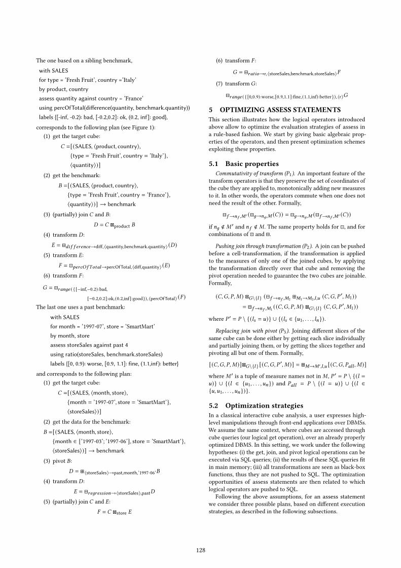
s e l e c t country , product , sum ( qu an t i t y ) as q u an t i t y2 from s a l e s s

j o i n cus tomer c on c . ckey = s . ckey4 j o i n p roduc t p on p . pkey = s . pkey

where type = ' Fre sh F r u i t ' and count ry = ' I t a l y '6 group by country , p roduc t

Listing 1: Getting the sales of fresh fruit products in Italy(Example 2.7)

cube is ⟨⟨Apple, Italy⟩, ⟨quantity = 100⟩⟩. The SQL formulationof 𝑞 on a star schema is given in Listing 1. □

3 COMPUTING AN ASSESSMENTBasically, the assessment of the values of a measure𝑚 in a cube𝐶 (called target cube) is done in three steps:

(1) the specification of a benchmark, i.e., a cube 𝐵 such that(i) its cells can be mapped one-to-one with the cells of 𝐶 ,and (ii) it has a measure𝑚′ representing the expected/ac-ceptable/normal performance of𝑚;

(2) the cell-wise comparison of𝑚 to𝑚′, which can be donein a basic way (e.g., algebraic/absolute/normalized differ-ence, percentage) or using more elaborate schemes (e.g.,z-scoring), possibly after applying some transformationsto𝑚 and𝑚′ (e.g., to compute derived measures);

(3) the characterization, or labeling, of the status of each cellof 𝐶 based on the result of the comparison; in the sim-plest case, this is done using a set of rules that map theresult of the comparison to a set of predefined labels (e.g.,“insufficient”, “excellent”, etc.).

3.1 BenchmarksThe specification of the benchmark is given by the analyst at theposing of the query. Thus, the question is “tell me how we aredoing with respect to this benchmark”.

A thorough comparison of a target cube 𝐶 against a bench-mark 𝐵 would require that the latter comes with the same levelmembers so that, for each cell of 𝐶 , we can map onto a cell of 𝐵.However, in practical cases, due to cube sparsity, there is no guar-antee that all cells can be mapped —especially if the benchmarkis retrieved from the web or other external data sources. Thus,in the following we provide a broad definition of the conditionsunder which two cubes are joinable, i.e., one of them can be usedas a benchmark to assess the other; in this definition, we will justrequire that the two cubes have the same group-by set.

Definition 3.1 (Cube Joinability). Let a target cube𝐶 over cubeschema C and a benchmark 𝐵 over B (where possibly, but notnecessarily, B = C) be given. Let 𝑞 = (𝐶0,𝐺𝐶 , 𝑃𝐶 , 𝑀𝐶 ) and𝑞′ = (𝐵0,𝐺𝐵, 𝑃𝐵, 𝑀𝐵) be the queries that resulted in 𝐶 and 𝐵,respectively. We say that 𝐶 and 𝐵 are joinable if

𝐺𝐶 = 𝐺𝐵

In OLAP terms, two cubes are joinable if a drill-across is possiblebetween 𝐶 and 𝐵.

Let C = (𝐻,𝑀) be the schema of the target cube 𝐶 , and 𝐶0 bethe detailed cube from which 𝐶 is derived. There are four typesof benchmarks we consider in our approach:

• Constant benchmarks. Here the user simply wants to assessthe cells of the target cube 𝐶 against some fixed value, astypically done with key performance indicators. In thiscase, the benchmark 𝐵 has schema B = (𝐻, ⟨𝑚𝑐𝑜𝑛𝑠𝑡 ⟩);

its cells have exactly the same coordinates as 𝐶 , and allof them store a constant value in𝑚𝑐𝑜𝑛𝑠𝑡 . The cell-to-cellmapping is trivially based on equality of coordinates.

• External benchmarks. Here the user’s goal is to assess thetarget cube against the data stored in a cube with schemaB = (𝐻 ′, 𝑀 ′). In principle, as long asB includes the group-by of the target cube (which ensures joinability), it is notnecessary to impose further constraints on B. However,for simplicity, in the following we will assume that theexternal benchmark has been reconciled with the targetcube so that 𝐻 = 𝐻 ′ and that all necessary transcodingsto level members have been applied (see e.g. [10] for anapproach that can be pursued to this end). Thus, also inthis case, mapping is based on equality of coordinates.

• Sibling benchmarks. The idea here is to compare the valuesof a measure in a slice on member 𝑢 ∈ 𝐷𝑜𝑚(𝑙) with thevalues of the same measure in another slice of 𝐶 relatedto a sibling member 𝑢𝑠𝑖𝑏 ∈ 𝐷𝑜𝑚(𝑙) (e.g., assess the salesof fruit in Italy with reference to those in France). In thiscase, the benchmark has the same schema C of the targetcube. Both cubes have the same group-by set, but whilethe cells in 𝐶 are those obtained from 𝐶0 using predicate𝑙 = 𝑢, those in 𝐵 are obtained from 𝐶0 using predicate𝑙 = 𝑢𝑠𝑖𝑏 . Then the cell-to-cell mapping is established byreplacing 𝑢 with 𝑢𝑠𝑖𝑏 in each coordinate of 𝐶 .

• Past benchmarks. In this case the user wants to assess thevalues taken by a measure𝑚 in some time slice with thevalues that can be predicted for𝑚 based on a number ofpast time slices. Like in the previous case, it is B = C. Thecells of 𝐵 have exactly the same coordinates as 𝐶 , but the(actual) values of𝑚 are replaced with the predicted ones.

Example 3.2. Let𝐶 be the derived cube obtained by query 𝑞 inExample 2.7 (total quantity sold by product and country for freshfruit products and Italy). An example of (joinable) sibling bench-mark is 𝐵 returned by 𝑞′, being 𝑞′ obtained from 𝑞 by replacingItaly with France. 𝐵 can be used to assess the sales of fresh fruitin Italy against those in France. The cell-to-cell mapping is estab-lished by replacing Italy with France; so, for instance, coordinate⟨Apple, Italy⟩ is mapped onto ⟨Apple, France⟩. □

3.2 Comparison & TransformationThe essence of assessment is to contrast the actual performanceagainst its expected value. Thus, the goal of this step is to providethe means to express and perform the evaluation of how far apartthe query result and the benchmark are. We refer to this actionas comparison to express the idea that this is not necessarilya simple measure difference. Modeling-wise, we assume that alibrary of comparison functions, all with signature 𝛿 : R × R→R, is available to the users. Practically, a cell-wise comparisonbetween measures of the target and benchmark can be easilyimplemented via different functions obeying the above signature,the simplest choice being a difference (either algebraic, or absolute,or normalized, etc.). In our examples, we will use two libraryfunctions of our system, named difference and ratio.

One could possibly expect that, once the target cube and thebenchmark have been obtained, their comparison is immediatelyapplicable. Interestingly, this is not always the case, since thecomparison may require the computation of derived measures.For instance, with reference to the SALES cube, comparing theactual profit for some given sales requires to compute a derivedmeasure as profit = storeSales− storeCost. Clearly, this requires

123

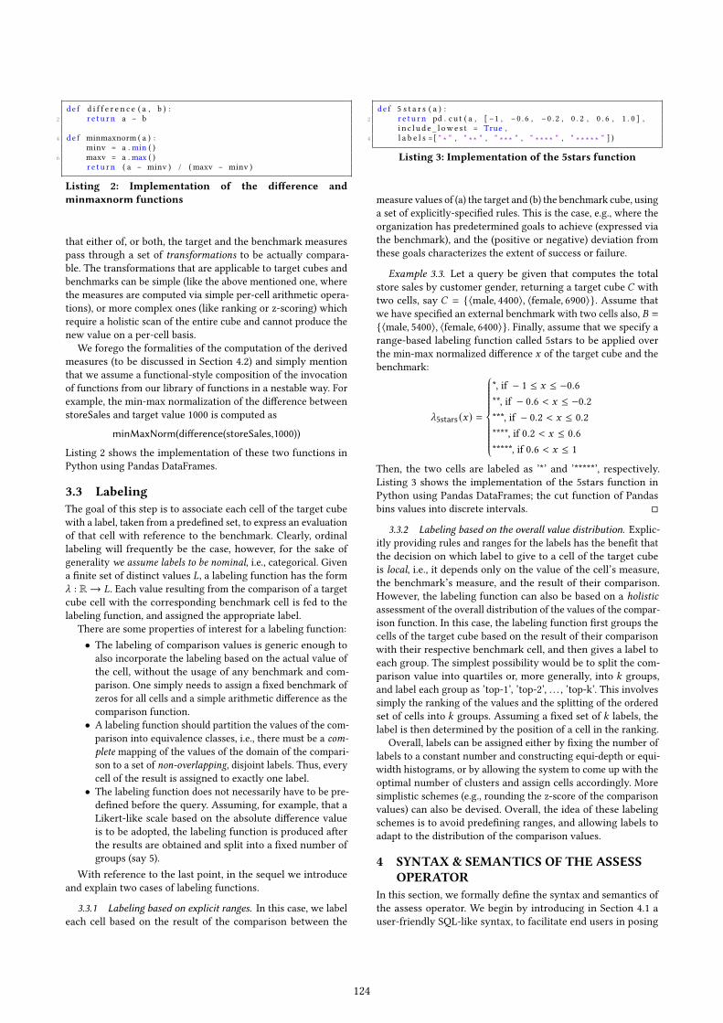
de f d i f f e r e n c e ( a , b ) :2 r e t u r n a − b

4 de f minmaxnorm ( a ) :minv = a . min ( )

6 maxv = a . max ( )r e t u r n ( a − minv ) / ( maxv − minv )

Listing 2: Implementation of the difference andminmaxnorm functions

that either of, or both, the target and the benchmark measurespass through a set of transformations to be actually compara-ble. The transformations that are applicable to target cubes andbenchmarks can be simple (like the above mentioned one, wherethe measures are computed via simple per-cell arithmetic opera-tions), or more complex ones (like ranking or z-scoring) whichrequire a holistic scan of the entire cube and cannot produce thenew value on a per-cell basis.

We forego the formalities of the computation of the derivedmeasures (to be discussed in Section 4.2) and simply mentionthat we assume a functional-style composition of the invocationof functions from our library of functions in a nestable way. Forexample, the min-max normalization of the difference betweenstoreSales and target value 1000 is computed as

minMaxNorm(difference(storeSales,1000))

Listing 2 shows the implementation of these two functions inPython using Pandas DataFrames.

3.3 LabelingThe goal of this step is to associate each cell of the target cubewith a label, taken from a predefined set, to express an evaluationof that cell with reference to the benchmark. Clearly, ordinallabeling will frequently be the case, however, for the sake ofgenerality we assume labels to be nominal, i.e., categorical. Givena finite set of distinct values 𝐿, a labeling function has the form_ : R→ 𝐿. Each value resulting from the comparison of a targetcube cell with the corresponding benchmark cell is fed to thelabeling function, and assigned the appropriate label.

There are some properties of interest for a labeling function:• The labeling of comparison values is generic enough toalso incorporate the labeling based on the actual value ofthe cell, without the usage of any benchmark and com-parison. One simply needs to assign a fixed benchmark ofzeros for all cells and a simple arithmetic difference as thecomparison function.

• A labeling function should partition the values of the com-parison into equivalence classes, i.e., there must be a com-plete mapping of the values of the domain of the compari-son to a set of non-overlapping, disjoint labels. Thus, everycell of the result is assigned to exactly one label.

• The labeling function does not necessarily have to be pre-defined before the query. Assuming, for example, that aLikert-like scale based on the absolute difference valueis to be adopted, the labeling function is produced afterthe results are obtained and split into a fixed number ofgroups (say 5).

With reference to the last point, in the sequel we introduceand explain two cases of labeling functions.

3.3.1 Labeling based on explicit ranges. In this case, we labeleach cell based on the result of the comparison between the

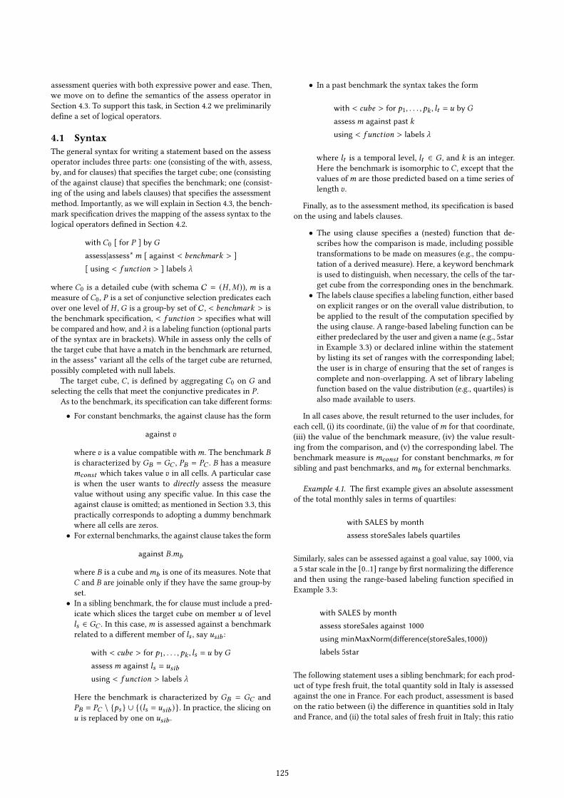
de f 5 s t a r s ( a ) :2 r e t u r n pd . cu t ( a , [ −1 , −0 . 6 , −0 . 2 , 0 . 2 , 0 . 6 , 1 . 0 ] ,

i n c l u d e _ l owe s t = True ,4 l a b e l s =[ " ∗ " , " ∗ ∗ " , " ∗ ∗ ∗ " , " ∗ ∗ ∗ ∗ " , " ∗ ∗ ∗ ∗ ∗ " ] )

Listing 3: Implementation of the 5stars function

measure values of (a) the target and (b) the benchmark cube, usinga set of explicitly-specified rules. This is the case, e.g., where theorganization has predetermined goals to achieve (expressed viathe benchmark), and the (positive or negative) deviation fromthese goals characterizes the extent of success or failure.

Example 3.3. Let a query be given that computes the totalstore sales by customer gender, returning a target cube 𝐶 withtwo cells, say 𝐶 = {⟨male, 4400⟩, ⟨female, 6900⟩}. Assume thatwe have specified an external benchmark with two cells also, 𝐵 =

{⟨male, 5400⟩, ⟨female, 6400⟩}. Finally, assume that we specify arange-based labeling function called 5stars to be applied overthe min-max normalized difference 𝑥 of the target cube and thebenchmark:

_5stars (𝑥) =

*, if − 1 ≤ 𝑥 ≤ −0.6**, if − 0.6 < 𝑥 ≤ −0.2***, if − 0.2 < 𝑥 ≤ 0.2****, if 0.2 < 𝑥 ≤ 0.6*****, if 0.6 < 𝑥 ≤ 1

Then, the two cells are labeled as ’*’ and ’*****’, respectively.Listing 3 shows the implementation of the 5stars function inPython using Pandas DataFrames; the cut function of Pandasbins values into discrete intervals. □

3.3.2 Labeling based on the overall value distribution. Explic-itly providing rules and ranges for the labels has the benefit thatthe decision on which label to give to a cell of the target cubeis local, i.e., it depends only on the value of the cell’s measure,the benchmark’s measure, and the result of their comparison.However, the labeling function can also be based on a holisticassessment of the overall distribution of the values of the compar-ison function. In this case, the labeling function first groups thecells of the target cube based on the result of their comparisonwith their respective benchmark cell, and then gives a label toeach group. The simplest possibility would be to split the com-parison value into quartiles or, more generally, into 𝑘 groups,and label each group as ’top-1’, ’top-2’, . . . , ’top-k’. This involvessimply the ranking of the values and the splitting of the orderedset of cells into 𝑘 groups. Assuming a fixed set of 𝑘 labels, thelabel is then determined by the position of a cell in the ranking.

Overall, labels can be assigned either by fixing the number oflabels to a constant number and constructing equi-depth or equi-width histograms, or by allowing the system to come up with theoptimal number of clusters and assign cells accordingly. Moresimplistic schemes (e.g., rounding the z-score of the comparisonvalues) can also be devised. Overall, the idea of these labelingschemes is to avoid predefining ranges, and allowing labels toadapt to the distribution of the comparison values.

4 SYNTAX & SEMANTICS OF THE ASSESSOPERATOR

In this section, we formally define the syntax and semantics ofthe assess operator. We begin by introducing in Section 4.1 auser-friendly SQL-like syntax, to facilitate end users in posing

124

assessment queries with both expressive power and ease. Then,we move on to define the semantics of the assess operator inSection 4.3. To support this task, in Section 4.2 we preliminarilydefine a set of logical operators.

4.1 SyntaxThe general syntax for writing a statement based on the assessoperator includes three parts: one (consisting of the with, assess,by, and for clauses) that specifies the target cube; one (consistingof the against clause) that specifies the benchmark; one (consist-ing of the using and labels clauses) that specifies the assessmentmethod. Importantly, as we will explain in Section 4.3, the bench-mark specification drives the mapping of the assess syntax to thelogical operators defined in Section 4.2.

with 𝐶0 [ for 𝑃 ] by 𝐺

assess|assess*𝑚 [ against < 𝑏𝑒𝑛𝑐ℎ𝑚𝑎𝑟𝑘 > ]

[ using < 𝑓 𝑢𝑛𝑐𝑡𝑖𝑜𝑛 > ] labels _

where 𝐶0 is a detailed cube (with schema C = (𝐻,𝑀)), 𝑚 is ameasure of 𝐶0, 𝑃 is a set of conjunctive selection predicates eachover one level of 𝐻 , 𝐺 is a group-by set of C, < 𝑏𝑒𝑛𝑐ℎ𝑚𝑎𝑟𝑘 > isthe benchmark specification, < 𝑓 𝑢𝑛𝑐𝑡𝑖𝑜𝑛 > specifies what willbe compared and how, and _ is a labeling function (optional partsof the syntax are in brackets). While in assess only the cells ofthe target cube that have a match in the benchmark are returned,in the assess* variant all the cells of the target cube are returned,possibly completed with null labels.

The target cube, 𝐶 , is defined by aggregating 𝐶0 on 𝐺 andselecting the cells that meet the conjunctive predicates in 𝑃 .

As to the benchmark, its specification can take different forms:

• For constant benchmarks, the against clause has the form

against 𝑣

where 𝑣 is a value compatible with𝑚. The benchmark 𝐵

is characterized by 𝐺𝐵 = 𝐺𝐶 , 𝑃𝐵 = 𝑃𝐶 . 𝐵 has a measure𝑚𝑐𝑜𝑛𝑠𝑡 which takes value 𝑣 in all cells. A particular caseis when the user wants to directly assess the measurevalue without using any specific value. In this case theagainst clause is omitted; as mentioned in Section 3.3, thispractically corresponds to adopting a dummy benchmarkwhere all cells are zeros.

• For external benchmarks, the against clause takes the form

against 𝐵.𝑚𝑏

where 𝐵 is a cube and𝑚𝑏 is one of its measures. Note that𝐶 and 𝐵 are joinable only if they have the same group-byset.

• In a sibling benchmark, the for clause must include a pred-icate which slices the target cube on member 𝑢 of level𝑙𝑠 ∈ 𝐺𝐶 . In this case,𝑚 is assessed against a benchmarkrelated to a different member of 𝑙𝑠 , say 𝑢𝑠𝑖𝑏 :

with < 𝑐𝑢𝑏𝑒 > for 𝑝1, . . . , 𝑝𝑘 , 𝑙𝑠 = 𝑢 by 𝐺

assess𝑚 against 𝑙𝑠 = 𝑢𝑠𝑖𝑏

using < 𝑓 𝑢𝑛𝑐𝑡𝑖𝑜𝑛 > labels _

Here the benchmark is characterized by 𝐺𝐵 = 𝐺𝐶 and𝑃𝐵 = 𝑃𝐶 \ {𝑝𝑠 } ∪ {(𝑙𝑠 = 𝑢𝑠𝑖𝑏 )}. In practice, the slicing on𝑢 is replaced by one on 𝑢𝑠𝑖𝑏 .

• In a past benchmark the syntax takes the form

with < 𝑐𝑢𝑏𝑒 > for 𝑝1, . . . , 𝑝𝑘 , 𝑙𝑡 = 𝑢 by 𝐺

assess𝑚 against past 𝑘

using < 𝑓 𝑢𝑛𝑐𝑡𝑖𝑜𝑛 > labels _

where 𝑙𝑡 is a temporal level, 𝑙𝑡 ∈ 𝐺 , and 𝑘 is an integer.Here the benchmark is isomorphic to 𝐶 , except that thevalues of𝑚 are those predicted based on a time series oflength 𝑣 .

Finally, as to the assessment method, its specification is basedon the using and labels clauses.

• The using clause specifies a (nested) function that de-scribes how the comparison is made, including possibletransformations to be made on measures (e.g., the compu-tation of a derived measure). Here, a keyword benchmarkis used to distinguish, when necessary, the cells of the tar-get cube from the corresponding ones in the benchmark.

• The labels clause specifies a labeling function, either basedon explicit ranges or on the overall value distribution, tobe applied to the result of the computation specified bythe using clause. A range-based labeling function can beeither predeclared by the user and given a name (e.g., 5starin Example 3.3) or declared inline within the statementby listing its set of ranges with the corresponding label;the user is in charge of ensuring that the set of ranges iscomplete and non-overlapping. A set of library labelingfunction based on the value distribution (e.g., quartiles) isalso made available to users.

In all cases above, the result returned to the user includes, foreach cell, (i) its coordinate, (ii) the value of𝑚 for that coordinate,(iii) the value of the benchmark measure, (iv) the value result-ing from the comparison, and (v) the corresponding label. Thebenchmark measure is𝑚𝑐𝑜𝑛𝑠𝑡 for constant benchmarks,𝑚 forsibling and past benchmarks, and𝑚𝑏 for external benchmarks.

Example 4.1. The first example gives an absolute assessmentof the total monthly sales in terms of quartiles:

with SALES by month

assess storeSales labels quartiles

Similarly, sales can be assessed against a goal value, say 1000, viaa 5 star scale in the [0..1] range by first normalizing the differenceand then using the range-based labeling function specified inExample 3.3:

with SALES by month

assess storeSales against 1000

using minMaxNorm(difference(storeSales,1000))

labels 5star

The following statement uses a sibling benchmark; for each prod-uct of type fresh fruit, the total quantity sold in Italy is assessedagainst the one in France. For each product, assessment is basedon the ratio between (i) the difference in quantities sold in Italyand France, and (ii) the total sales of fresh fruit in Italy; this ratio

125

is computed using library function 𝑝𝑒𝑟𝑐𝑂 𝑓𝑇𝑜𝑡𝑎𝑙 .

with SALES

for type = ’Fresh Fruit’, country =’Italy’by product, country

assess quantity against country = ’France’using percOfTotal(difference(quantity, benchmark.quantity))

labels {[-inf, -0.2): bad, [-0.2,0.2]: ok, (0.2, inf]: good},

Finally, in the next statement we use a past benchmark; specifi-cally, we assess the sales of a specific store in July 1997 againstthe past four months:

with SALES

for month = ’1997-07’, store = ’SmartMart’by month, store

assess storeSales against past 4

using ratio(storeSales, benchmark.storeSales)

labels {[0, 0.9): worse, [0.9, 1.1]: fine, (1.1,inf): better}

□

4.2 Logical operatorsThis section introduces the logical aspects behind the differentsteps of the evaluation of an assess statement, formulated aslogical operators. Note that our aim is not to propose a logicallanguage for manipulating cubes (such languages exist, see e.g.[2]) but to describe specific cube manipulations required to logi-cally optimize assess statements. In particular, we do not detailthe classical (roll-up, etc.) cube manipulations.

We recall from Section 2 that a cube is defined as a partialfunction that maps coordinates into tuples of measures. For acube 𝐶 and a coordinate 𝛾 such that 𝐶 (𝛾) = 𝑡 , we denote with𝑐 = ⟨𝛾, 𝑡⟩ the cell defined by 𝐶 (𝛾) and we abusively note 𝑐 ∈ 𝐶 .We define operators that respect the closure property, in the sensethat they operate on cubes and specify cubes.

Get. The first basic operator consists of obtaining the result ofa cube query. Given a cube 𝐶 over a schema C = (𝐻,𝑀), a set ofselection predicates 𝑃 and a group-by set𝐺 of C, the get operatorcorresponds to the cube query 𝑞 = (𝐶,𝐺, 𝑃,𝑀), is denoted by[𝑞], and defines the derived cube being the result of 𝑞. Note that[(𝐶,𝐺0, ∅, 𝑀)] is simply noted [𝐶] in what follows. Besides, thederived cube returned by get can be renamed using the notation[(𝐶,𝐺, 𝑃,𝑀)] → 𝑛𝑎𝑚𝑒 .

Join ⊠. The join operation is essential for putting together thetarget cube (𝐶1) and the benchmark (𝐶2). In OLAP terms this is adrill-across operation, or join applied to cubes.

Let 𝐶1 and 𝐶2 be two joinable cubes over schemas C1 andC2. As already stated, we assume for simplicity that the twocubes share the same hierarchies, so that C1 = (𝐻,𝑀1) andC2 = (𝐻,𝑀2).

𝐶1 ⊠𝐶2 = {⟨𝛾, (𝑡, 𝑡 ′)⟩|⟨𝛾, 𝑡⟩ ∈ 𝐶1, ⟨𝛾, 𝑡 ′⟩ ∈ 𝐶2}The schema of the resulting cube is (𝐻, (𝑀1, 𝑀2)).

We also define a version of join where we allow partial joiningin the sense that join is made on a subset of the levels of 𝐻 .Formally:

𝐶1 ⊠𝑙1,...,𝑙𝑚 𝐶2 = {⟨𝛾, (𝑡, 𝑡1, . . . , 𝑡𝑝 )⟩|

⟨𝛾, 𝑡⟩ ∈ 𝐶1, ⟨𝛾 𝑗 , 𝑡 𝑗 ⟩ ∈ 𝐶2, 𝛾 |𝑙1,...,𝑙𝑚 = 𝛾𝑗

|𝑙1,...,𝑙𝑚, 𝑗 ∈ [1, . . . , 𝑝]}

Italy

Apple ‹quan%ty  = 100›

Pear ‹quan%ty  = 90›

Lemon ‹quan%ty  = 30›

France

Apple ‹quan%ty  = 150›

Pear ‹quan%ty  = 110›

Lemon ‹quan%ty  = 20›

Italy

Apple ‹quan%ty  = 100, benchmark.quan%ty = 150›

Pear ‹quan%ty  = 90, benchmark.quan%ty = 110›

Lemon ‹quan%ty  = 30, benchmark.quan%ty = 20›

Italy

Apple ‹quan%ty  = 100, benchmark.quan%ty = 150, diff  = −50›

Pear ‹quan%ty  = 90, benchmark.quan%ty = 110, diff  = −20›

Lemon ‹quan%ty  = 30, benchmark.quan%ty = 20, diff  = 10›

Italy

Apple ‹quan%ty  = 100, benchmark.quan%ty = 150, diff  = −50, percOfTotal  = −0.23›

Pear ‹quan%ty  = 90, benchmark.quan%ty = 110, diff  = −20, percOfTotal  = −0.09›

Lemon ‹quan%ty  = 30, benchmark.quan%ty = 20, diff  = 10, percOfTotal  = 0.05›

Italy France

Apple ‹quan%ty  = 100› ‹quan%ty  = 150›

Pear ‹quan%ty  = 90› ‹quan%ty  = 110›

Lemon ‹quan%ty  = 30› ‹quan%ty  = 20›

Italy

Apple ‹quan%ty  = 100, benchmark.quan%ty = 150, diff  = −50, percOfTotal  = −0.23, label = bad›

Pear ‹quan%ty  = 90, benchmark.quan%ty = 110, diff  = −20, percOfTotal  = −0.09, label = ok›

Lemon ‹quan%ty  = 30, benchmark.quan%ty = 20, diff  = 10, percOfTotal  = 0.05, label = ok›

C B

D

E

F

G

C'

Italy

Apple ‹quan%ty  = 100, qtyFrance  = 150›

Pear ‹quan%ty  = 90, qtyFrance  = 110›

Lemon ‹quan%ty  = 30, qtyFrance  = 20›

D'

Figure 1: Derived cubes resulting from the application oflogical operators for the sibling intention in Example 4.5

Note that, differently from the (natural) join defined above, thispartial join is not commutative.

Finally, the assess* syntactical variant (that also returns thenon-matching cells of the target cube) uses a left-outer join𝐶1 ∗ ⊠ 𝐶2 where non-matching cells are completed with nullvalues.

Example 4.2. Figure 1 shows the results, 𝐶 and 𝐵, of the fol-lowing get operations:

𝐶 =[(SALES, ⟨product, country⟩,{type = ’Fresh Fruit’, country = ’Italy’},⟨quantity⟩)]

𝐵 =[(SALES, ⟨product, country⟩,{type = ’Fresh Fruit’, country = ’France’},⟨quantity⟩)] → benchmark

(cube 𝐵 is given alias benchmark) and the result of their partialjoin, 𝐷 = 𝐶 ⊠product 𝐵. □

Cell-Transform ⊟. This operator specifies a cell-at-a-time oper-ation that takes a cube and a function, and outputs a cube wherea new measure is added, containing the value of the functionapplied over the measure(s). Let C = (𝐻,𝑀) be the schema ofcube 𝐶 with group-by set 𝐺 , and𝑀 be a subtuple of𝑀 . Let 𝑓 bea function defined on a tuple of parameters compatible with𝑀 ;then the cell-transformation operation operated by 𝑓 returns acube defined by:

⊟𝑓→𝑛𝑎𝑚𝑒,𝑀

(𝐶) = {⟨𝛾, (𝑡, ⟨𝑓 (𝑀)⟩)⟩ | ⟨𝛾, 𝑡⟩ ∈ 𝐶}

The schema of the resulting cube is (𝐻, (𝑀, ⟨𝑛𝑎𝑚𝑒⟩)), where𝑛𝑎𝑚𝑒 is the derived measure returned by 𝑓 .

126

Italy

Apple ‹quan%ty  = 100›

Pear ‹quan%ty  = 90›

Lemon ‹quan%ty  = 30›

France

Apple ‹quan%ty  = 150›

Pear ‹quan%ty  = 110›

Lemon ‹quan%ty  = 20›

Italy

Apple ‹quan%ty  = 100, benchmark.quan%ty = 150›

Pear ‹quan%ty  = 90, benchmark.quan%ty = 110›

Lemon ‹quan%ty  = 30, benchmark.quan%ty = 20›

Italy

Apple ‹quan%ty  = 100, benchmark.quan%ty = 150, diff  = −50›

Pear ‹quan%ty  = 90, benchmark.quan%ty = 110, diff  = −20›

Lemon ‹quan%ty  = 30, benchmark.quan%ty = 20, diff  = 10›

Italy

Apple ‹quan%ty  = 100, benchmark.quan%ty = 150, diff  = −50, percOfTotal  = −0.23›

Pear ‹quan%ty  = 90, benchmark.quan%ty = 110, diff  = −20, percOfTotal  = −0.09›

Lemon ‹quan%ty  = 30, benchmark.quan%ty = 20, diff  = 10, percOfTotal  = 0.05›

Italy France

Apple ‹quan%ty  = 100› ‹quan%ty  = 150›

Pear ‹quan%ty  = 90› ‹quan%ty  = 110›

Lemon ‹quan%ty  = 30› ‹quan%ty  = 20›

Italy

Apple ‹quan%ty  = 100, benchmark.quan%ty = 150, diff  = −50, percOfTotal  = −0.23, label = bad›

Pear ‹quan%ty  = 90, benchmark.quan%ty = 110, diff  = −20, percOfTotal  = −0.09, label = ok›

Lemon ‹quan%ty  = 30, benchmark.quan%ty = 20, diff  = 10, percOfTotal  = 0.05, label = ok›

C B

D

E

F

G

C'

Italy

Apple ‹quan%ty  = 100, qtyFrance  = 150›

Pear ‹quan%ty  = 90, qtyFrance  = 110›

Lemon ‹quan%ty  = 30, qtyFrance  = 20›

D'

Figure 2: Example of application of the pivot operator

H-Transform ⊡. This operator considers holistic (H) transfor-mations, in the sense that computing a new measure value foreach cell of cube 𝐶 requires to know all the cells of 𝐶 .

Let again𝑀 be a subtuple of𝑀 as above. In this case, function𝑓 operates on a tuple of parameters compatible with𝑀 and on aset of tuples. The H-transformation of 𝐶 operated by 𝑓 returns acube defined by:

⊡𝑓→𝑛𝑎𝑚𝑒,𝑀

(𝐶) = {⟨𝛾, (𝑡, ⟨𝑓 (𝑀,𝐶)⟩)⟩ | ⟨𝛾, 𝑡⟩ ∈ 𝐶}

The schema of the resulting cube is (𝐻, (𝑀, ⟨𝑛𝑎𝑚𝑒⟩)), where𝑛𝑎𝑚𝑒 is the extra measure returned by 𝑓 .

Example 4.3. The following cell-transformation extends cube𝐷 with a derived measure storing their difference:

𝐸 = ⊟𝑑𝑖 𝑓 𝑓 𝑒𝑟𝑒𝑛𝑐𝑒→diff, ⟨quantity,benchmark.quantity⟩ (𝐷)Then, cube 𝐹 is obtained from 𝐸 by applying an H-transformationas follows:

𝐹 = ⊡𝑝𝑒𝑟𝑐𝑂𝑓𝑇𝑜𝑡𝑎𝑙→percOfTotal, ⟨diff,quantity⟩ (𝐸)where holistic function 𝑝𝑒𝑟𝑐𝑂 𝑓𝑇𝑜𝑡𝑎𝑙 operates on a tuple of twoparameters 𝑎 and 𝑏 and computes, for each cell, the ratio between𝑎 and the sum of 𝑏 over all cells. □

Pivot ⊞. This operator takes a cube including a set of 𝑘 slicesof some level 𝑙 (a cube slice is the set of cells corresponding to onesingle member of a level), among which only one slice for a givenmember 𝑢𝑘 ∈ 𝐷𝑜𝑚(𝑙) is returned. Each coordinate 𝛾 of this slicein the returned cube is associated with its initial tuple of measures𝑡 , concatenated with all the 𝑝 measures𝑀 = ⟨𝑚1, . . . ,𝑚𝑝 ⟩ of allits 𝑘 − 1 neighbor coordinates 𝛾 ′ in the initial set of 𝑘 slices. Thenew measures are renamed 𝑛𝑎𝑚𝑒1, . . . , 𝑛𝑎𝑚𝑒𝑝 . Formally, givencube 𝐶 with schema C = (𝐻,𝑀), let 𝑢1, . . . , 𝑢𝑘 ∈ 𝐷𝑜𝑚(𝑙) bethe members of 𝑙 on which the slices are defined. Let 𝑢𝑘 be thereference slice for pivoting. Then

⊞⟨𝑚1→𝑛𝑎𝑚𝑒1,...,𝑚𝑝→𝑛𝑎𝑚𝑒𝑝 ⟩,𝑙,𝑢𝑘 (𝐶) =

{⟨𝛾, (𝑡, ⟨𝑣11, . . . , 𝑣1𝑘−1, . . . , 𝑣

𝑝

1 , . . . , 𝑣𝑝

𝑘−1⟩)⟩|⟨𝛾, 𝑡⟩ ∈ 𝐶,𝛾 |𝑙 = 𝑢𝑘 , ⟨𝛾 ′, 𝑡 ′⟩ ∈ 𝐶,𝛾 ′|𝑙 = 𝑢𝑖 ,

𝛾 |𝐺\𝑙 = 𝛾 ′|𝐺\𝑙, 𝑡 ′|

𝑚𝑗= 𝑣

𝑗𝑖, 𝑖 ∈ [1, 𝑘 − 1], 𝑗 ∈ [1, 𝑝]}

where the 𝑡 ’s are tuples of measure values. The schema of the re-sulting cube is (𝐻, (𝑀,𝑛𝑎𝑚𝑒1, . . . , 𝑛𝑎𝑚𝑒𝑝 )) where in turn𝑛𝑎𝑚𝑒 =

⟨𝑚1, . . . ,𝑚𝑘−1⟩.

Example 4.4. Figure 2 shows the result𝐶 ′ of the following getoperator:

𝐶 ′ =[(SALES, ⟨product, country⟩,{type = ’Fresh Fruit’, country ∈ {’Italy’, ’France’}},⟨quantity⟩)]

Cube 𝐶 ′ includes two slices for country. By applying the follow-ing pivot operator:

𝐷 ′ = ⊞⟨quantity⟩→qtyFrance,country,’Italy’ (𝐶 ′)

a cube𝐷 ′ is obtained that includes only the reference slice (’Italy’),with an extra measure qtyFrance. □

4.3 SemanticsAssume the expression of the assess operator as defined in Section4.1:

with 𝐶0 [ for 𝑃 ] by 𝐺

assess𝑚 [ against < 𝑏𝑒𝑛𝑐ℎ𝑚𝑎𝑟𝑘 > ]

[ using < 𝑓 𝑢𝑛𝑐𝑡𝑖𝑜𝑛 > ] labels _

In terms of the logical operators introduced in Section 4.2, let

(1) ⊡Δ, · (·) be the composition of the comparison/transforma-tion functions denoted by the using clause.

(2) ⊡_, · (·) be the transformation that applies the labeling func-tion denoted by the labels clause.

Without loss of generalization, we assume that the functions thatare used for the comparison and the labeling are holistic. Clearly,the application of cell-based functions is also possible (and mostwelcome for efficiency and optimization purposes).

The semantics of an assess statement is defined as

⊡_→𝑚_,𝑚Δ (⊡Δ→𝑚Δ,𝑀(𝐶))

where the definition of cube𝐶 depends on the type of benchmarkused, which in turn is determined by the form taken by theagainst clause as explained in Section 4.1:

• Constant benchmark: 𝐶 = [(𝐶0,𝐺, 𝑃,𝑀)].• External benchmark 𝐵: 𝐶 = [(𝐶0,𝐺, 𝑃,𝑀)] ⊠ [𝐵]• Sibling benchmark:

𝐶 = [(𝐶0,𝐺, 𝑃,𝑀)] ⊠𝐺\𝑙𝑠 [(𝐶0,𝐺, 𝑃𝐵, 𝑀)] → benchmark

where 𝑃𝐵 = 𝑃 \ {(𝑙𝑠 = 𝑢)} ∪ {(𝑙𝑠 = 𝑢𝑠𝑖𝑏 )}.• Past benchmark:

𝐶 = [(𝐶0,𝐺, 𝑃,𝑀)]⊠𝐺\𝑙𝑡 (⊟𝑟𝑒𝑔𝑟𝑒𝑠𝑠𝑖𝑜𝑛→𝑀′,𝑀 (⊞𝑀→𝑀′,𝑙𝑡 ,𝑢 (

[(𝐶0,𝐺, 𝑃𝐵, 𝑀)] → benchmark)))

where 𝑃𝐵 = 𝑃 \ {(𝑙𝑡 = 𝑢)}∪ {(𝑙𝑡 ∈ {𝑢1, . . . , 𝑢𝑘 }), members𝑢1, . . . , 𝑢𝑘 are predecessors of𝑢 for level 𝑙𝑡 , and 𝑟𝑒𝑔𝑟𝑒𝑠𝑠𝑖𝑜𝑛is a time series prediction function.

Note that, in the assess* variant, the inner join is replaced bya left-outer join. In all cases, the resulting cube has schema(𝐻, ⟨𝑚,𝑚𝐵,𝑚Δ,𝑚_⟩) The benchmark measure𝑚𝐵 is𝑚𝑐𝑜𝑛𝑠𝑡 forconstant benchmarks,𝑚 for sibling and past benchmarks, and𝑚𝑏 for external benchmarks.

Example 4.5. Consider again some of the statements of Exam-ple 4.1. The first one relies on a constant benchmark:

with SALES by month

assess storeSales labels quartiles,

and corresponds to the logical expression:

⊡𝑞𝑢𝑎𝑟𝑡𝑖𝑙𝑒𝑠, ⟨storeSales⟩ ( [(SALES, ⟨month⟩, ∅, ⟨storeSales⟩)])

127

The one based on a sibling benchmark,

with SALES

for type = ’Fresh Fruit’, country =’Italy’by product, country

assess quantity against country = ’France’using percOfTotal(difference(quantity, benchmark.quantity))

labels {[-inf, -0.2): bad, [-0.2,0.2]: ok, (0.2, inf]: good},

corresponds to the following plan (see Figure 1):(1) get the target cube:

𝐶 =[(SALES, ⟨product, country⟩,{type = ’Fresh Fruit’, country = ’Italy’},⟨quantity⟩)]

(2) get the benchmark:

𝐵 =[(SALES, ⟨product, country⟩,{type = ’Fresh Fruit’, country = ’France’},⟨quantity⟩)] → benchmark

(3) (partially) join 𝐶 and 𝐵:

𝐷 = 𝐶 ⊠product 𝐵

(4) transform 𝐷 :

𝐸 = ⊟𝑑𝑖 𝑓 𝑓 𝑒𝑟𝑒𝑛𝑐𝑒→diff, ⟨quantity,benchmark.quantity⟩ (𝐷)(5) transform 𝐸:

𝐹 = ⊡𝑝𝑒𝑟𝑐𝑂𝑓𝑇𝑜𝑡𝑎𝑙→percOfTotal, ⟨diff,quantity⟩ (𝐸)(6) transform 𝐹 :

𝐺 = ⊟𝑟𝑎𝑛𝑔𝑒 ( { [−inf,−0.2) :bad,

[−0.2,0.2]:ok,(0.2,inf]:good}), ⟨percOfTotal⟩ (𝐹 )The last one uses a past benchmark:

with SALES

for month = ’1997-07’, store = ’SmartMart’by month, store

assess storeSales against past 4

using ratio(storeSales, benchmark.storeSales)

labels {[0, 0.9): worse, [0.9, 1.1]: fine, (1.1,inf): better}

and corresponds to the following plan:(1) get the target cube:

𝐶 =[(SALES, ⟨month, store⟩,{month = ’1997-07’, store = ’SmartMart’},⟨storeSales⟩)]

(2) get the data for the benchmark:

𝐵 =[(SALES, ⟨month, store⟩,{month ∈ [’1997-03’; ’1997-06’], store = ’SmartMart’},⟨storeSales⟩)] → benchmark

(3) pivot 𝐵:

𝐷 = ⊞⟨storeSales⟩→past,month,’1997-06’𝐵

(4) transform 𝐷 :

𝐸 = ⊟𝑟𝑒𝑔𝑟𝑒𝑠𝑠𝑖𝑜𝑛→⟨storeSales⟩,past𝐷

(5) (partially) join 𝐶 and 𝐸:

𝐹 = 𝐶 ⊠store 𝐸

(6) transform 𝐹 :

𝐺 = ⊟𝑟𝑎𝑡𝑖𝑜→r, ⟨storeSales,benchmark.storeSales⟩𝐹

(7) transform 𝐺 :

⊟𝑟𝑎𝑛𝑔𝑒 ( { [0,0.9) :worse, [0.9,1.1]:fine,(1.1,inf) :better}), ⟨r⟩𝐺

5 OPTIMIZING ASSESS STATEMENTSThis section illustrates how the logical operators introducedabove allow to optimize the evaluation strategies of assess ina rule-based fashion. We start by giving basic algebraic prop-erties of the operators, and then present optimization schemesexploiting these properties.

5.1 Basic propertiesCommutativity of transform (𝑃1). An important feature of the

transform operators is that they preserve the set of coordinates ofthe cube they are applied to, monotonically adding newmeasuresto it. In other words, the operators commute when one does notneed the result of the other. Formally,

⊟𝑓→𝑛𝑓 ,𝑀′ (⊟𝑔→𝑛𝑔,𝑀 (𝐶)) = ⊟𝑔→𝑛𝑔,𝑀 (⊟𝑓→𝑛𝑓 ,𝑀

′ (𝐶))

if 𝑛𝑔 ∉ 𝑀 ′ and 𝑛𝑓 ∉ 𝑀 . The same property holds for ⊡, and forcombinations of ⊡ and ⊟.

Pushing join through transformation (𝑃2). A join can be pushedbefore a cell-transformation, if the transformation is appliedto the measures of only one of the joined cubes, by applyingthe transformation directly over that cube and removing thepivot operation needed to guarantee the two cubes are joinable.Formally,

(𝐶,𝐺, 𝑃,𝑀) ⊠𝐺\{𝑙 } (⊟𝑓→𝑛𝑓 ,𝑀2 ⊞𝑀1→𝑀2,𝑙,𝑢 (𝐶,𝐺, 𝑃 ′, 𝑀1))= ⊟𝑓→𝑛𝑓 ,𝑀1 ((𝐶,𝐺, 𝑃,𝑀) ⊠𝐺\{𝑙 } (𝐶,𝐺, 𝑃 ′, 𝑀1))

where 𝑃 ′ = 𝑃 \ {(𝑙𝑠 = 𝑢)} ∪ {(𝑙𝑠 ∈ {𝑢1, . . . , 𝑙𝑛}).

Replacing join with pivot (𝑃3). Joining different slices of thesame cube can be done either by getting each slice individuallyand partially joining them, or by getting the slices together andpivoting all but one of them. Formally,

[(𝐶,𝐺, 𝑃,𝑀)]⊠𝐺\{𝑙 } [(𝐶,𝐺, 𝑃 ′, 𝑀)] = ⊞𝑀→𝑀′,𝑙,𝑢 [(𝐶,𝐺, 𝑃𝑎𝑙𝑙 , 𝑀)]

where 𝑀 ′ is a tuple of measure names not in 𝑀 , 𝑃 ′ = 𝑃 \ {(𝑙 =𝑢)} ∪ {(𝑙 ∈ {𝑢1, . . . , 𝑢𝑛}) and 𝑃𝑎𝑙𝑙 = 𝑃 \ {(𝑙 = 𝑢)} ∪ {(𝑙 ∈{𝑢,𝑢1, . . . , 𝑢𝑛})}.

5.2 Optimization strategiesIn a classical interactive cube analysis, a user expresses high-level manipulations through front-end applications over DBMSs.We assume the same context, where cubes are accessed throughcube queries (our logical get operation), over an already properlyoptimized DBMS. In this setting, we work under the followinghypotheses: (i) the get, join, and pivot logical operations can beexecuted via SQL queries; (ii) the results of these SQL queries fitin main memory; (iii) all transformations are seen as black-boxfunctions, thus they are not pushed to SQL. The optimizationopportunities of assess statements are then related to whichlogical operators are pushed to SQL.

Following the above assumptions, for an assess statementwe consider three possible plans, based on different executionstrategies, as described in the following subsections.

128

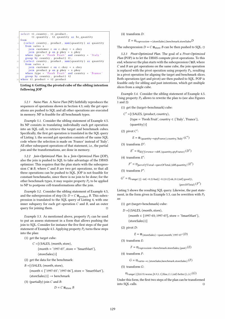
s e l e c t t 1 . country , t 1 . product ,2 t 1 . quan t i t y , t 2 . q u an t i t y as b c _ qu an t i t y

from4 ( s e l e c t country , product , sum ( qu an t i t y ) as q u an t i t y

from s a l e s s6 j o i n cus tomer c on c . ckey = s . ckey

j o i n produc t p on p . pkey = s . pkey8 where type = ' Fre sh F r u i t ' and count ry = ' I t a l y '

group by country , p roduc t ) t1 ,10 ( s e l e c t country , product , sum ( qu an t i t y ) as q u an t i t y

from s a l e s s12 j o i n cus tomer c on c . ckey = s . ckey

j o i n produc t p on p . pkey = s . pkey14 where type = ' Fre sh F r u i t ' and count ry = ' France '

group by country , p roduc t ) t 216 where t 1 . p roduc t = t 2 . p roduc t

Listing 4: Getting the pivoted cube of the sibling intentionfollowing JOP

5.2.1 Naive Plan. A Naive Plan (NP) faithfully reproduces thesequences of operations shown in Section 4.3; only the get oper-ations are pushed to SQL and all other operations are executedin memory. NP is feasible for all benchmark types.

Example 5.1. Consider the sibling statement of Example 4.5.Its NP consists in translating individually each get operationinto an SQL call, to retrieve the target and benchmark cubes.Specifically, the first get operation is translated in the SQL queryof Listing 1; the second get operation consists of the same SQLcode where the selection is made on ’France’ instead of ’Italy’.All other subsequent operations of that statement, i.e., the partialjoin and the transformations, are done in memory.

5.2.2 Join-Optimized Plan. In a Join-Optimized Plan (JOP),also the join is pushed to SQL to take advantage of the DBMSoptimizer. This requires that the plan starts with the subexpres-sion 𝐶 ⊠ 𝐵, where 𝐶 and 𝐵 are two get operations, so that allthree operations can be pushed to SQL. JOP is not feasible forconstant benchmarks, since there is no join to be done; for theother benchmark types, it may require property 𝑃2 to be appliedto NP to postpone cell-transformations after the join.

Example 5.2. Consider the sibling statement of Example 4.5,and the subexpression of step (3): 𝐷 = 𝐶 ⊠product 𝐵. This subex-pression is translated to the SQL query of Listing 4, with oneinner subquery for each get operation 𝐶 and 𝐵, and an outerquery for joining them. □

Example 5.3. As mentioned above, property 𝑃2 can be usedto put an assess statement in a form that allows pushing thejoin to SQL. Consider for instance the five first steps of the paststatement of Example 4.5. Applying property 𝑃2 turns these stepsinto the plan:

(1) get the target cube:

𝐶 =[(SALES, ⟨month, store⟩,{month = ’1997-07’, store = ’SmartMart’},⟨storeSales⟩)]

(2) get the data for the benchmark:

𝐵 =[(SALES, ⟨month, store⟩,{month ∈ [’1997-03’; ’1997-06’], store = ’SmartMart’},⟨storeSales⟩)] → benchmark

(3) (partially) join 𝐶 and 𝐵:

𝐷 = 𝐶 ⊠store 𝐵

(4) transform 𝐷 :

𝐸 = ⊟𝑟𝑒𝑔𝑟𝑒𝑠𝑠𝑖𝑜𝑛→⟨storeSales⟩,benchmark.storeSales𝐷

The subexpression 𝐷 = 𝐶 ⊠store 𝐵 can be then pushed to SQL. □

5.2.3 Pivot-Optimized Plan. The goal of a Pivot-OptimizedPlan (POP) is to let the DBMS compute pivot operations. To thisend, whenever the plan starts with the subexpression𝐶⊠𝐵, where𝐶 and 𝐵 are get operations on the same cube, the join operationis replaced with the pivot operation using property 𝑃3, resultingin a pivot operation for aligning the target and benchmark slices.Both operations (get and pivot) are then pushed to SQL. POP isfeasible only for sibling and past intentions, which get multipleslices from a single cube.

Example 5.4. Consider the sibling statement of Example 4.5.Using property 𝑃3 allows to rewrite the plan to (see also Figures1 and 2):

(1) get the (target+benchmark) cube:

𝐶 ′ =[(SALES, ⟨product, country⟩,{type = ’Fresh Fruit’, country ∈ {’Italy’, ’France’},⟨quantity⟩)]

(2) pivot 𝐶 ′:

𝐸 = ⊞⟨quantity→qtyFrance⟩,country,’Italy’ (𝐶 ′)

(3) transform 𝐷 ′:

𝐸 ′ = ⊟𝑑𝑖 𝑓 𝑓 𝑒𝑟𝑒𝑛𝑐𝑒→diff, ⟨quantity,qtyFrance⟩ (𝐷 ′)

(4) transform 𝐸 ′:

𝐹 ′ = ⊡𝑝𝑒𝑟𝑐𝑂𝑓𝑇𝑜𝑡𝑎𝑙→percOfTotal, ⟨diff,quantity⟩ (𝐸 ′)

(5) transform 𝐹 ′:

𝐺 ′ = ⊟𝑟𝑎𝑛𝑔𝑒 ( { [−inf,−0.2) :bad, [−0.2,0.2]:ok,(0.2,inf]:good}),

⟨percOfTotal⟩ (𝐹 ′)

Listing 5 shows the resulting SQL query. Likewise, the past state-ment, in the form given in Example 5.3, can be rewritten with 𝑃3as:

(1) get (target+benchmark) cube:

𝐷 =[(SALES, ⟨month, store⟩,{month ∈ [1997-03; 1997-07], store = ’SmartMart’},⟨storeSales⟩)]

(2) pivot 𝐷 :

𝐸 = ⊞⟨storeSales⟩→past,month,’1997-07’ (𝐷)

(3) transform 𝐸:

𝐹 = ⊟𝑟𝑒𝑔𝑟𝑒𝑠𝑠𝑖𝑜𝑛→benchmark.storeSales, ⟨past⟩ (𝐸)

(4) transform 𝐹 :

𝐺 = ⊟𝑟𝑎𝑡𝑖𝑜→r, ⟨storeSales,benchmark.storeSales⟩ (𝐹 )

(5) transform 𝐺 :

⊟𝑟𝑎𝑛𝑔𝑒 ( { [0,0.9) :worse, [0.9,1.1]:fine,(1.1,inf) :better}), ⟨r⟩ (𝐺)

Under this form, the first two steps of the plan can be transformedinto SQL calls. □

129

s e l e c t ' I t a l y ' as country , product ,2 quan t i t y , b c _ qu an t i t y

from4 ( s e l e c t country , product , sum ( qu an t i t y ) as q u an t i t y

from s a l e s s6 j o i n cus tomer c on c . ckey = s . ckey

j o i n produc t p on p . pkey = s . pkey8 where type = ' Fre sh F r u i t '

and count ry in ( ' I t a l y ' , ' France ' )10 group by country , p roduc t )

p i v o t (12 sum ( qu an t i t y ) f o r count ry

in ( ' I t a l y ' as quan t i t y , ' France ' as b c _qu an t i t y )14 )

where qu an t i t y i s not n u l l and b c _qu an t i t y i s not n u l l

Listing 5: Getting the pivoted cube of the sibling intentionfollowing POP

Table 1: Formulation effort for different intentions

Constant External Sibling PastSQL: 481 989 1169 1954

Python: 7006 6193 6309 7049Total: 7487 7182 7478 9003assess: 143 260 270 254

6 EXPERIMENTSTo test our approach, we implemented the assess operator relyingon the simple multidimensional engine described in [6], whichuses multidimensional metadata to rewrite OLAP queries on astar schema stored in Oracle 11g DBMS. Post-processing of theresults (e.g., to apply transformations) is then done via off-the-shelf Python Scikit-learn over Pandas DataFrames. All tests wererun on an Intel(R) Core(TM)i7-6700 CPU@3.40GHz CPU with8GB RAM.

The prototype was tested against the Star Schema Benchmark(SSB) cube, described by four hierarchies; please refer to [14]for the logical schema of the SSB dataset. As commonly donein OLAP settings, primary and foreign keys were indexed usingB-Trees, and materialized views were created to improve perfor-mances. The experiments are focused on four assess statementsof different types, henceforth referred to as Constant, External,Sibling, and Past, respectively.

6.1 Formulation effortThe first goal of our experiments is to evaluate the saving in user’seffort when writing an assess statement over the one necessaryto obtain the same result using plain SQL and Python. To thisend we adopt the simple metric proposed in [11], where theASCII character length is used as as a proxy for the effort it takesto craft a query. The results are shown in Table 1. For SQL andPython we considered the code generated by our prototype whenfollowing the less complex plan. Nevertheless, as expected, thetotal formulation effort using SQL+Python is, for each intentiontype, more than one order of magnitude larger than using assessstatements.

6.2 Efficiency and scalabilityOur second experimental goal is to evaluate the efficiency ofour approach in executing (i) different types of intentions, (ii)with different execution plans, and (iii) on cubes with differentcardinalities. To achieve (iii) we generated three detailed SSB

Table 2: Target cube cardinalities for each intention typeapplied to each detailed cube

𝑆𝑆𝐵1 𝑆𝑆𝐵10 𝑆𝑆𝐵100Constant 1.2 · 105 1.2 · 106 1.2 · 107External 2.4 · 104 2.5 · 105 2.5 · 106Sibling 2.4 · 104 2.5 · 105 2.5 · 106

Past 1.5 · 103 1.6 · 104 1.6 · 105

Table 3: Minimum execution times (in seconds) for differ-ent intentions (in parentheses, the corresponding execu-tion times for NP)

𝑆𝑆𝐵1 𝑆𝑆𝐵10 𝑆𝑆𝐵100Constant 0.60 (0.60) 6.77 (6.77) 45.14 (45.14)External 0.27 (0.31) 2.38 (2.60) 32.86 (35.60)Sibling 0.32 (0.42) 3.69 (4.97) 49.61 (99.93)

Past 1.20 (3.21) 11.72 (30.93) 118.25 (321.11)

cubes, namely 𝑆𝑆𝐵1, 𝑆𝑆𝐵10, and 𝑆𝑆𝐵100, with different scale fac-tors resulting in the following cardinalities:

|𝑆𝑆𝐵1 | =6 · 106

|𝑆𝑆𝐵10 | =6 · 107

|𝑆𝑆𝐵100 | =6 · 108

Note that the cardinality of each cube is equal to the numberof tuples in the corresponding fact table. Since the by and forclauses of each assess statement are not changed, scaling up thecardinality of the detailed cube implies that also the cardinalityof the target cube scales up as shown in Table 2. To reduce theimpact of caching, each assess statement was executed five timeson each detailed cube, and the execution times were averaged.

Figure 3 shows, on a logarithmic scale, the times in seconds forexecuting the Constant, External, Sibling, and Past intentions us-ing the NP, JOP, and POP plans, for increasing cube cardinalities.As to Constant, assessing a target cube of 1.2 · 107 tuples (derivedby querying 𝑆𝑆𝐵100) takes about 45 seconds, mostly employedto get the data from the DBMS. Note that, since this assessmentdoes not require the retrieval of a benchmark cube, only NP isfeasible. As to External, the only possible plans are NP and JOP(POP is not feasible here), with JOP providing the best perfor-mance. As to Sibling and Past, POP performs the best, taking50 seconds and 118 seconds, respectively. Being based on thepivot operator, POP gets in both cases the target cube and thebenchmark at once by retrieving the slices required together. Inother words, POP avoids the join between the target cube and thebenchmark, a time-consuming operation for NP and JOP. Overall,NP has the worst performance, since (i) it requires to separatelyget both cubes and join them into main memory, and (ii) it mayload into main memory unnecessary data (i.e., the tuples thatwill not match in the join). Overall, we can conclude that (i) JOP,when applicable, outperforms NP, and (ii) POP, when applicable,outperforms JOP and NP. This is summarized in Table 3 which,for each benchmark type, compares the best performance withthe one of the naive execution strategy. Remarkably, this tablealso clearly shows that our approach scales linearly for all theintentions.

Our last experimental goal is to understand which are themost expensive execution steps, i.e., those for which there isroom for further optimizations. The overall execution time for

130

SSB1 SSB10 SSB100

100

101

Tim

e (s

)Constant

SSB1 SSB10 SSB100

100

101

Tim

e (s

)

External

SSB1 SSB10 SSB100

100

101

102

Tim

e (s

)

Sibling

SSB1 SSB10 SSB100

100

101

102

Tim

e (s

)

Past

NPJOPPOP

Figure 3: Execution times for increasing cardinalities of the target cube 𝐶

SSB1 SSB10 SSB10010 3

10 2

10 1

100

101

102

103

Tim

e (s

)

NP

SSB1 SSB10 SSB10010 3

10 2

10 1

100

101

102

103

Tim

e (s

)

JOP

SSB1 SSB10 SSB10010 3

10 2

10 1

100

101

102

103

Tim

e (s

)

POP

Get C Get B Get C + B Trans. Join Comp. Label

Figure 4: Breakdown of the execution time of the Past intention for increasing cardinalities of the target cube 𝐶

an intention can be broken down into the time necessary to (1)get the target cube, (2) get the benchmark, (3) transform thetwo cubes (e.g., to apply regression in past benchmarks), (4) jointhem, (5) compute the comparison/transformation, and (6) labelthe result. This breakdown is shown in Figure 4 for each plan andwith increasing cube cardinalities. We focus on the Past intention,that is the most complex one since forecasting measure valuesrequires to compute a regression. First of all, we observe thatthe execution times for comparison and labeling are in the orderof milliseconds. Thus, not surprisingly, they are negligible withrespect to the time necessary to get and join the cubes. For allthree plans, transformation is the most time-consuming step,since linear regression has to be applied to huge numbers oftuples. As to the time for accessing data, note that:

• NP brings both the target 𝐶 and benchmark 𝐵 cubes intomain memory to join them; the cost for this main-memoryjoin is lower than the ones for getting the two cubes, butstill not negligible. The cost for the pivot operation iscounted as transformation.

• JOP pushes the join to SQL; thus, in this case the cost forthe join is counted together with the one for getting𝐶 +𝐵.The cost for the pivot operation is counted as transforma-tion.

• POP replaces the join with a pivot operation and pushesit to SQL, thus, the cost of pivot here is part of the cost forgetting 𝐶 + 𝐵.

7 RELATEDWORK7.1 OLAP models and operatorsOLAP comes with a large number of proposals on its foundationsand operators, all of which slowly converged towards the coreideas of cubes, dimensions, dimension hierarchies, and levels aswell as operators like roll-up, drill-down, slice, drill-across duringthe late ’90s. To avoid overcrowding the discussion, we refer theinterested reader to an excellent survey [16].

Over the years, several operators have been proposed to com-plement the fundamental ones. The DIFF operator [17] returnsthe set of tuples that most successfully describe the difference ofvalues between two cells of a cube that are given as input. Thesame author also describes a method that profiles the explorationof a user and uses the Maximum Entropy principle to recommendwhich unvisited parts of the cube can be the most surprising ina subsequent query [18]. Finally, the RELAX operator allows toverify whether a pattern observed at a certain level of detail ispresent at a coarser level of detail too [19].

In a different line of research, prediction cubes are proposedwith the characteristic property that each of the cells comes witha model that is trained to produce a predictive model with datathat correspond to that cell [5]. Then, a comparison betweenmodel and actual value is also possible, assessing the model’saccuracy. Also, the Shrink operator [9, 15] has been proposed toreduce the result size of a query with minimal loss of informationvalue via the calculated fusion of data slices.

Alternative operators have also been proposed in the Cinecubesmethod [7, 8]. The goal of this effort is to facilitate automatedreporting, given an original OLAP query as input. To achieve thispurpose two operators (expressed as acts) are proposed, namely,(a) put-in-context, i.e., compare the result of the original queryto query results over similar, sibling values; and (b) give-details,where drill-downs of the original query’s groupers are performed.

Compared to the previous proposals, our work on the explicitintroduction of an assess operator differs in the fundamentalproblem it addresses. The works of Sarawagi are mostly of ex-planatory rather than assessment nature. Similarly, predictioncubes are trying to assess the impact of a set of predictor at-tributes on a class label in the context of a data cube, via anintroduced model for their relationship —again, the emphasis ison trying to explain what we see rather than trying to provideassessments and labels on the comparison of the assessment.The Shrink operator is intended to compress without losing too

131

much information. The Cinecubes approach introduces an auto-matically invoked model of assessment in its put-in-context act;this is indeed a first form of assessment, although not tunable orexplicitly invoked by the user.

7.2 The Intentional Analytics ModelThe IAM for OLAP was introduced in [20]. Later this proposalwas significantly extended [21]. The main idea behind the inten-tional model for OLAP is that OLAP models need to be extendedwith (a) new operators, (b) altering of the definition of a queryresult, (c) introducing highlights to annotate the answers. Toaddress the first requirement, the traditional roll-ups and drill-downs operators were complemented with operators that pertainto the intention of the user towards the data —i.e., what is thereason why the user poses the query. The original, large set ofoperators (including operators like verify and analyze) was latersolidified and formalized into five operators, namely, describe,assess, explain, predict, and suggest [21]. The result of a queryis also redefined as a combination of data and KDD models thatare applied over the data. Also, the resulting data and modelsare evaluated with respect to their interestingness to producehighlights, i.e., subsets of the data that provide the most of novelinformation to the user. The foundations of the model can belinked to Bloom’s taxonomy and Anderson and Krathwohl’s re-finement to it [13, 22], which organize cognitive tasks as: (a)remembering, (b) understanding, (c) applying a procedure, (d)analyzing (component interrelationships), (e) evaluating (withrespect to criteria and standards), and (f) creating.

Although the IAM acts as an all-encompassing framework fordefining new operators, results, and highlights for OLAP, thegoal of the previous works was not go down into the detailsof each operator, but rather to dictate templates on what kindof algebraic operators we can introduce. The particularities ofthe describe operator (supporting the understanding process inBloom’s framework) were further explored [4]. The current paperextends the originally proposed assess operator (in turn, inspiredby the put-in-context operator) in significantly deeper ways,as it comes with several alternatives that were not obviouslyexpressed in the original work [21], as well as with the syntax ofan SQL-like language and optimization techniques.

8 CONCLUSIONSIn this paper we have introduced the assess operator to auto-matically evaluate and characterize the result of a cube query interms of labels given to the single cells based on their compar-ison with a benchmark. We have provided several alternativesfor specifying benchmarks, comparison, and labeling schemes.Finally, we have discussed alternative plans for the execution ofassess statements showing that their performance is perfectly inline with the right time requirement of analysis sessions.

Our future work on the assess operator will develop in differ-ent directions:

• Consider cube schemas including descriptive propertiesof levels (e.g., the population of a country). Introducingproperties will enable users to express more complex state-ments, e.g., to compare per capita sales of different coun-tries.

• Devise strategies for effectively completing partial assessstatements, for instance, ones where the against, using or

benchmark clauses are not specified by the user. Interest-ingly, this could require different possibilities to be testedand ranked based on their expected interest for the user.

• Enhance the expressiveness of the assess operator by con-sidering more complex labeling functions (e.g., functionsbased on ranges that depend not only on comparison val-ues of cells, but also on their coordinates) and additionaltypes of benchmarks (for instance to let the sales of milkbe assessed against those of drinks, i.e., against an ancestorof milk in the roll-up order).

• Investigate the relevant properties of our logical operatorsand develop a cost-based optimization strategy.

REFERENCES[1] Serge Abiteboul, Richard Hull, and Victor Vianu. 1995. Foundations of

Databases. Addison-Wesley.[2] Rakesh Agrawal, Ashish Gupta, and Sunita Sarawagi. 1997. Modeling Multidi-

mensional Databases. In Proceedings of ICDE. Birmingham, UK, 232–243.[3] Leilani Battle, Michael Stonebraker, and Remco Chang. 2013. Dynamic re-

duction of query result sets for interactive visualizaton. In Proceedings ofInternational Conference on Big Data. Santa Clara, CA, USA, 1–8.

[4] Antoine Chédin, Matteo Francia, Patrick Marcel, Verónika Peralta, and StefanoRizzi. 2020. The Tell-Tale Cube. In Proceedings of ADBIS. Lyon, France, 204–218.

[5] Bee-Chung Chen, Lei Chen, Yi Lin, and Raghu Ramakrishnan. 2005. PredictionCubes. In Proceedings of VLDB. Trondheim, Norway, 982–993.

[6] Matteo Francia, Enrico Gallinucci, and Matteo Golfarelli. 2020. TowardsConversational OLAP. In Proceedings of DOLAP. Copenhagen, Denmark, 6–15.

[7] Dimitrios Gkesoulis and Panos Vassiliadis. 2013. CineCubes: cubes as moviestars with little effort. In Proceedings of DOLAP. San Francisco, CA, USA, 3–10.

[8] Dimitrios Gkesoulis, Panos Vassiliadis, and Petros Manousis. 2015. CineCubes:Aiding data workers gain insights from OLAP queries. Inf. Syst. 53 (2015),60–86.

[9] Matteo Golfarelli, Simone Graziani, and Stefano Rizzi. 2014. Shrink: An OLAPoperation for balancing precision and size of pivot tables. Data Knowl. Eng.93 (2014), 19–41.

[10] Matteo Golfarelli, Federica Mandreoli, Wilma Penzo, Stefano Rizzi, and ElisaTurricchia. 2012. OLAP query reformulation in peer-to-peer data warehousing.Inf. Syst. 37, 5 (2012), 393–411.

[11] Shrainik Jain, Dominik Moritz, Daniel Halperin, Bill Howe, and Ed Lazowska.2016. SQLShare: Results from a Multi-Year SQL-as-a-Service Experiment. InProceedings of SIGMOD. San Francisco, CA, USA, 281–293.

[12] Sean Kandel, Andreas Paepcke, Joseph M. Hellerstein, and Jeffrey Heer. 2012.Enterprise Data Analysis and Visualization: An Interview Study. IEEE Trans.Vis. Comput. Graph. 18, 12 (2012), 2917–2926.

[13] David R. Krathwohl. 2002. A Revision of Bloom’s Taxonomy: An Overview.Theory Into Practice 41, 4 (2002), 212–218.

[14] Patrick E. O’Neil, Elizabeth J. O’Neil, Xuedong Chen, and Stephen Revilak.2009. The Star Schema Benchmark and Augmented Fact Table Indexing. InProceedings of TPCTC. Lyon, France, 237–252.

[15] Stefano Rizzi, Matteo Golfarelli, and Simone Graziani. 2015. An OLAM Oper-ator for Multi-Dimensional Shrink. Int. J. of Data Warehousing and Mining 11,3 (2015), 68–97.

[16] Oscar Romero and Alberto Abelló. 2007. On the Need of a Reference Algebrafor OLAP. In Proceedings of DaWaK. Regensburg, Germany, 99–110.

[17] Sunita Sarawagi. 1999. Explaining Differences inMultidimensional Aggregates.In Proceedings of VLDB. Edinburgh, Scotland, 42–53.

[18] Sunita Sarawagi. 2000. User-Adaptive Exploration of Multidimensional Data.In Proceedings of VLDB. Cairo, Egypt, 307–316.

[19] Gayatri Sathe and Sunita Sarawagi. 2001. Intelligent Rollups in Multidimen-sional OLAP Data. In Proceedings of VLDB. Roma, Italy, 531–540.

[20] Panos Vassiliadis and Patrick Marcel. 2018. The Road to Highlights is Pavedwith Good Intentions: Envisioning a Paradigm Shift in OLAP Modeling. InProceedings of DOLAP. Vienna, Austria.

[21] Panos Vassiliadis, Patrick Marcel, and Stefano Rizzi. 2019. Beyond Roll-Up’sand Drill-Down’s: An Intentional Analytics Model to Reinvent OLAP. Infor-mation Systems 85 (2019), 68–91.

[22] Leslie Owen Wilson. 2016. Anderson and Krathwohl - Bloom’s Taxonomy Re-vised. thesecondprinciple.com/teaching-essentials/beyond-bloom-cognitive-taxonomy-revised/.

[23] Kanit Wongsuphasawat, Yang Liu, and Jeffrey Heer. 2019. Goals, Process,and Challenges of Exploratory Data Analysis: An Interview Study. CoRRabs/1911.00568 (2019).

132