Improving the interface stability of cross-linked films by ink ...
138
Improving the interface stability of cross-linked films by ink formulation in printed organic light emitting diodes Hibon, Pauline (2020) DOI (TUprints): https://doi.org/10.25534/tuprints-00014138 Lizenz: CC-BY-SA 4.0 International - Creative Commons, Namensnennung, Weitergabe un- ter gleichen Bedingungen Publikationstyp: Dissertation Fachbereich: 11 Fachbereich Material- und Geowissenschaften Quelle des Originals: https://tuprints.ulb.tu-darmstadt.de/14138
-
Upload
khangminh22 -
Category
Documents
-
view
0 -
download
0
Transcript of Improving the interface stability of cross-linked films by ink ...
Improving the interface stability of cross-linked films by inkformulation in printed organic light emitting diodes
Hibon, Pauline(2020)
DOI (TUprints): https://doi.org/10.25534/tuprints-00014138
Lizenz:
CC-BY-SA 4.0 International - Creative Commons, Namensnennung, Weitergabe un-ter gleichen Bedingungen
Publikationstyp: Dissertation
Fachbereich: 11 Fachbereich Material- und Geowissenschaften
Quelle des Originals: https://tuprints.ulb.tu-darmstadt.de/14138
Improving the interface stability of
cross-linked films by ink formulation
in printed organic light emitting diodes
at the Material Science Faculty
of the Technische Universität Darmstadt
submitted in fulfilment of the requirements for the degree of Doctor-Engineer (Dr.-Ing.)
Doctoral thesis by M.Eng. Paulie Hibon, born in Reims (France)
First assessor: Prof. Dr. Heinz von Seggern Second assessor: Prof. Dr. Edgar Dörsam
Darmstadt 2020 (year of the viva voce)

Pauline Hibon: Improving the interface stability of cross-linked films by ink formulation in printed organic light emitting diodes Darmstadt, Technische Universität Darmstadt, Year thesis published in TUprints 2020 Date of the viva voce 11.09.2020 Published under CC BY-SA 4.0 International https://creativecommons.org/licenses/

i Table of content
Table of content
Table of content i
Erklärung zur Dissertation i
1. Introduction 1
2. Theory 3
2.1. OLED introduction and architecture 3
2.1.1. Material deposition process 7
2.1.2. Soluble organic semiconductors 8
2.2. Inkjet printing of thin films 10
2.2.1. Instrumentation and operation mode 10
2.2.2. Print-heads 11
2.2.3. Challenges 12
2.3. IJP inks: Polymer solutions 15
2.3.1. Polymer solubility profile 15
2.3.2. Size of polymer chain in solution 16
2.3.3. Interaction between polymer and solvent 18
3. Investigated System and Methods 21
3.1. Materials 21
3.1.1. Hole transport materials 21
3.1.2. Inkjet printing solvents 22
3.1.3. Ink formulations 24
3.1.4. Solution characterisation 24
3.2. Processing of an inkjet printed layer 28
3.2.1. Inkjet printer 28
3.2.2. Printing substrates 29
3.2.3. Film formation process 30
3.2.4. Film thickness measurement 32
3.2.5. Polymer bulk properties 33
3.2.6. Polymer film properties 34
3.3. Electronic device 38
3.3.1. Carrier mobility in hole transport layer 39
3.3.2. Bipolar devices 40
ii Table of content
3.3.3. Characterisation of OLED devices 41
4. Characterisation of polymer solutions based on experimental and empirical descriptions 45
4.1. Polymer-solvent affinity 46
4.1.1. Experimental determination of polymer-solvent affinity 46
4.1.2. Empirical observations 48
4.2. Polymer size in solution 55
4.2.1. Radius of gyration 55
4.2.2. Volume fraction 56
4.2.3. Polymer coil diameter 57
4.3. Conclusion on polymer solution characterisation 58
5. Polymer cross-linking in bulk material and thin films 61
5.1. Cross-linking of X-Po in powder without solvent 61
5.1.1. Styrene cross-linking reaction 61
5.1.2. Cross-linking reaction enthalpy 63
5.2. Significance of cross-linking in polymer solution 65
5.2.1. Rheology investigation 65
5.2.2. Variation of species’ size in solution 67
5.2.3. Cross-linking reaction enthalpy in solution 70
5.3. Polymer cross-linking in film 71
5.3.1. Sample preparation 71
5.3.2. Stability of thin films against solvent exposure 75
5.3.3. Degree of cross-linking 80
5.3.4. Variation of optical properties 82
5.4. Conclusion on polymer cross-linking in bulk material and thin films 84
6. Inkjet printing of cross-linkable HTL in OLED devices 87
6.1. Inkjet printing of hole transport ink 87
6.1.1. HTL surface energy 88
6.1.2. EML film formation 89
6.2. Influence of hole transport ink on OLED devices 91
6.2.1. Carrier mobility in HTL 91
6.2.2. Bipolar devices 92
6.3. Conclusion on cross-linking HTL in OLED devices 98
7. Summary 101
8. Outlook 103

iii Table of content
Acknowledgments 105
Curriculum Vitae 107
Table of Figures 109
Table of Tables 115
List of Abbreviations 117
Formula Directory 119
List of References 123


Erklärung zur Dissertation
Erklärung zur Dissertation
Hiermit versichere ich, die vorliegende Dissertation ohne Hilfe Dritter nur mit den angegebenen
Quellen und Hilfsmitteln angefertigt zu haben. Alle Stellen, die aus Quellen entnommen wurden, sind
als solche kenntlich gemacht. Diese Arbeit hat in gleicher oder ähnlicher Form noch keiner
Prüfungsbehörde vorgelegen. Eine Promotion wurde bisher noch nicht versucht.
Darmstadt, den 05.10.2020
(Pauline Hibon)

1.Introduction 1
1. Introduction
The first display in form of a cathode ray tube was demonstrated in 1897 by the Nobel-prize physicist
and inventor Karl Ferdinand Braun. The basic operation consists of an electron gun firing electrons
onto a phosphor-coated screen leading to image formation. Colours appeared in 1954 and it was the
most popular display technology utilised for television and computer monitors until the arrival of liquid
crystal displays in 1968, which gradually replaced the cathode ray tubes. Electroluminescent displays
were not commercially ready until the late 1970’s when Sharp Corporation introduced the so-called
alternating-current-thin-film approach.1 Organic (i.e., carbon-based) electroluminescence emanated in
the late 1980’s with the first Organic Light Emitting Diode (OLED) by Tang et al.2 The use of
polymers as electrically conductive materials was revealed by inadvertence in the late 1970’s by
Shirakawa and co-workers at the Tokyo University.3 The advantage of using polymers as electronic
materials is that they combine the electronic properties of semiconductors with the ease of
processability of plastics. The first conjugated polymer-based OLED, also called PLED was
demonstrated in 1990 at the Cavendish laboratory using poly(phenylene vinylene) (PPV).4 It
established that light emitting devices could be made with organic and solution-processed materials.5
Thus, OLED has become an established technology in the display market because of their very high
luminous efficiency, low power consumption, and long lifetime thanks to complex multilayer
architectures.2, 4, 6-8
Display application is boosted by a race for higher performance, such as higher resolution and lower
price. Unlike thermal evaporation,9 solution processes are lowering production costs due to high
material usage and ease of scalability for different sizes.10 For solution-processed OLED display
fabrication techniques, inkjet printing (IJP) has the potential to be the state-of-the-art technology for
high resolution R-G-B pixel definition.11-14 However, some challenges related to the soluble OLED
technology have to be understood and overcome, e.g., the influence of different molecular orientations
and the intermixing between layers.15
Intermixing between successive solution-processed layers was shown to damage the previously
deposited layer and to be hard to prevent.16-18 Therefore, interface control remains a top challenge of
solution-processed OLEDs since device performance heavily relies on it. Such undefined interfaces are
detrimental to OLED performance (e.g., shifted emission zone),19 but also for quantum dot based
PLEDs.20 Due to the nanometre thickness of the layers composing these devices, even the smallest
interface mixing affects their performance.
To control interfaces, several approaches such as orthogonal solvent21-22 or cross-linked materials23-25
have been intensively studied. Dummy buffer layers have proved to stop intermixing but add an
additional layer to an already complex architecture26. For preventing this effect fast drying was used
to shorten the diffusion time of the solvents in the wet state.27-28
Orthogonal solvents are of interest especially when low molecular weight or non-cross-linkable
materials are used. Finding such solvent can be complicated, since two consecutive layer materials
must show a significant difference in their polarity or solubility profile.29-31 Besides the
solubility/orthogonality challenge, other criteria have to be taken into account such as solvent/print-
head compatibility, low toxicity of the solvent, low amount of impurities that could diminish device
performance, and impact of the solvent itself on the overall device. In this work, the focus was set on
2 1.Introduction
cross-linked materials. Material characterisation is generally performed by a lab-scale soluble process,
i.e., spin coating. Unlike IJP, the method of choice for display fabrication, spin coating offers a fast-
drying speed to the processed layer, and drying speed is a driving force for reducing strong mixing of
two subsequent layers. For this reason, film stability of an inkjet deposited and cross-linked layer
against subsequent exposure to a suitable inkjet printing solvent has been investigated. Impact of ink
solvent on solution-cast thin film properties has already been studied for polyvinyl acetate films.32-33
The objective was to determine the influence of the ink solvent on the cross-linking degree of a polymer
in thin films.
This work concentrates on the stability of a hole transport layer (HTL) against a subsequent solution
deposition of an emissive layer (EML) ink. The emissive material is composed of small molecules
known to be very mobile in multilayer stacks. Sharp interfaces between the HTL and the EML were
proven essential to guarantee an efficient exciton confinement within the EML layer by avoiding
shifted emission zones.34 Thus, OLED device efficiency is directly affected by the interface sharpness
between HTL and EML.35
The theoretical principles used in this thesis are described in Chapter 2. Chapter 3 illustrates the
detailed experimental conditions and settings. In this thesis, the studied polymer solutions were first
characterised to differentiate them from one another by describing the polymer-solvent interaction in
solution (Chapter 4). The interactions were determined experimentally and based on empirical
descriptions, like Kramer equation, Huggins equation and Solomon Cuita equation. Thereafter, the
polymer cross-linking reaction was examined in the bulk material and in the films (Chapter 5).
Differential scanning calorimetry (DSC) was used to quantify the efficiency of polymer cross-linking
reactions in powder and in films processed from different solvents. The stability of polymer films
against solvent exposure was inspected with the aim to identify the impact of ink solvent on the film
stability. An understanding of the correlation between cross-linking reaction efficiency in film and film
stability against solvent exposure was drawn. Finally, OLED devices were produced with the aim to
study the influence of HTL ink solvent on optical and electrical properties of the devices (Chapter 6).
A summary and outlook constitute the final Chapter 7 of this thesis.
2.1. OLED introduction and architecture 3
2. Theory
2.1. OLED introduction and architecture
Electroluminescence in organic materials was first demonstrated in 1963 by Pope et al.36 and in 1965
by Helfrich and Schneider37 with a single layer OLED. They observed green light emission from a
layer of an anthracene crystal sandwiched between two electrodes biased with 400 V. When voltage is
applied across the two electrodes, an electrical current is generated, and charge carriers of opposite
polarity are introduced into the layers which upon recombination converted to light. This proof-of-
concept OLED, composed of a transparent anode, a combined transport and emissive layer and a
metallic cathode, suffered from high voltage and poor power-conversion efficiency. In 1987, Tang and
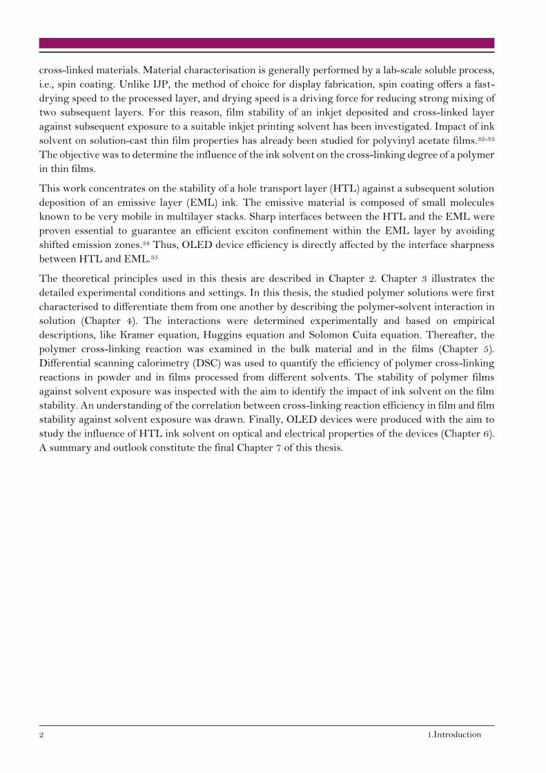
Van Slyke presented the first multilayer OLED stack2 introducing an ultra-thin monopolar hole
transport layer (HTL) in combination with an ultra-thin electron transport layer (ETL) as seen in
Figure 2.1 which acted simultaneously as emissive layer between the anode and cathode resulting in
lower driving voltages and improved electroluminescent emission efficiency. Since then, more
advanced stack designs were used to create OLED devices with more and more functional layers.38
The overall stack thickness is usually in the range of few hundred of nanometres.
Figure 2.1: Development of OLED stacks from
two functional layers to a multilayer structure.
(left) Two layers OLED from Tang and van Slyke
published in 1987. (right) A complex OLED
structure commonly used in recent devices. It
consists of charge carrier injection layers (HIL,
EIL), transport layers (HTL, ETL), blocking layers
(HBL, EBL) located on either sides of the central
emission layer (EML).
Modern OLEDs consist of multiple thin films of organic layers sandwiched between two electrodes.
In order to enhance the injection of charge carriers from the electrodes into the organic layers, a hole
(/electron) injection layer (HIL/EIL) is added followed by a hole (/electron) transport layer
(HTL/ETL). Efficient confinement of hole and electrons in the emissive layer can be improved by hole
(/electron) blocking layers (HBL/EBL). This avoids the loss of electrons and holes from the emissive
layer and leads to an efficiency increase. The anode has to be transparent to guarantee the light output
and commonly consists of indium tin oxide (ITO). The cathode is normally reflective and made of
metals such as aluminium.
Working principle of OLED
The semiconductor properties of organic materials, no matter whether small molecules or polymers,
are based on conjugated bonds, i.e., π-orbitals “filled with” delocalised electrons, which impact the
electronic and optical properties of the materials. An overlap of atomic orbitals results in a set of new

4 2.Theory
orbitals called bonding and anti-bonding molecular orbitals. Electrons in π-orbitals provide a lower
stabilisation than those in σ bond. Figure 2.2a shows the two different types of bond. As a consequence,
the energy gap between bonding (π) and anti-bonding molecular orbital (π*) is smaller than in the case
of σ bonding. The highest occupied 𝜋 state is called HOMO and the lowest unoccupied molecular
orbital (𝜋∗) is called LUMO. The energy gap (Eg) of a molecule is determined by the energy difference
between HOMO and LUMO. An energetic representation of these bond types is depicted in Figure
2.2b.
Figure 2.2: a) Schematic representation of pz-orbitals, σ- and π-bonds between two carbon atoms.
b) Energy levels of bonding (𝜋)and antibonding orbitals (𝜋∗).
Positive charges, designated as holes, are injected from the Fermi level of the anode into the HOMO
of the neighbouring organic layer, and the electrons are injected from the Fermi level of the cathode
into the LUMO of the neighbouring organic layer under applied positive bias voltage V0. The voltage
induced electric field forces electrons and holes to move towards each other to preferentially recombine
in the EML resulting in photon emission. Thanks to a high HTL LUMO and a low ETL HOMO, the
electrons and the holes are confined in the EML. The energy gap Eg of the emissive species in the EML
determines the frequency of the emitted light, i.e., the emitted light colour. The working principle of
an OLED under electrical field is represented in Figure 2.3.
Figure 2.3: Schematic representation of the fundamental
processes of an OLED in operation. (1) Charge carrier injection.
(2) Charge carrier transport. (3) Recombination of the charge
carriers to excitons. (4) Emission of light.
2.1. OLED introduction and architecture 5
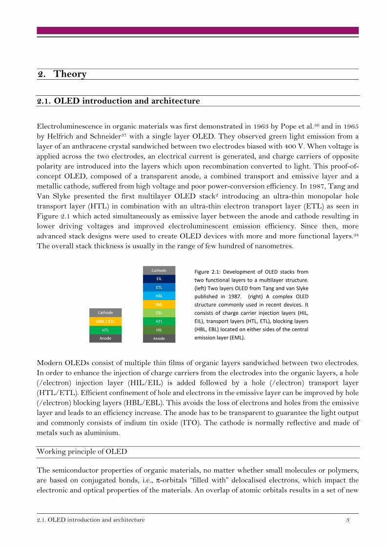
Charge injection
Charge carrier injection corresponds to the introduction of holes and electrons into the HOMO and
the LUMO of the organic layer from the anode and the cathode, respectively. However, for charge
carrier injection to happen, there are injection barriers Eb,e for electrons and Eb,h for holes that must be
overcome, as shown in Figure 2.4.
Figure 2.4: Energy diagram of injection process from the
electrodes in an OLED device.
When applying an external electric field to the OLED device, the electron and hole injection barriers
can be overcome. Alignment of Fermi level of the cathode and the anode takes place with the LUMO
and the HOMO levels of the adjacent molecules, respectively, resulting in charges injection.39 Reducing
the injection barriers from the electrodes to the organic layers can be achieved by choosing high work
function anodes, whereas the cathode consists mainly of metals with low work function. Another
strategy is to select the organic materials so that the HOMO (/LUMO) of the HIL (/EIL) lays closely
to the Fermi level of the anode (/cathode).
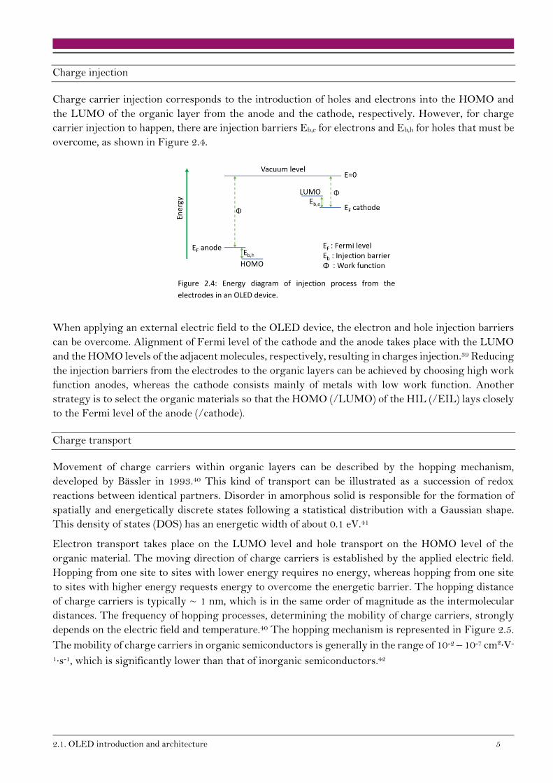
Charge transport
Movement of charge carriers within organic layers can be described by the hopping mechanism,
developed by Bässler in 1993.40 This kind of transport can be illustrated as a succession of redox
reactions between identical partners. Disorder in amorphous solid is responsible for the formation of
spatially and energetically discrete states following a statistical distribution with a Gaussian shape.
This density of states (DOS) has an energetic width of about 0.1 eV.41
Electron transport takes place on the LUMO level and hole transport on the HOMO level of the
organic material. The moving direction of charge carriers is established by the applied electric field.
Hopping from one site to sites with lower energy requires no energy, whereas hopping from one site
to sites with higher energy requests energy to overcome the energetic barrier. The hopping distance
of charge carriers is typically ~ 1 nm, which is in the same order of magnitude as the intermolecular
distances. The frequency of hopping processes, determining the mobility of charge carriers, strongly
depends on the electric field and temperature.40 The hopping mechanism is represented in Figure 2.5.
The mobility of charge carriers in organic semiconductors is generally in the range of 10-2 – 10-7 cm²∙V-
1∙s-1, which is significantly lower than that of inorganic semiconductors.42
6 2.Theory
Figure 2.5: Hopping mechanism responsible for charge
transport in OLED device.
Charge recombination and light generation
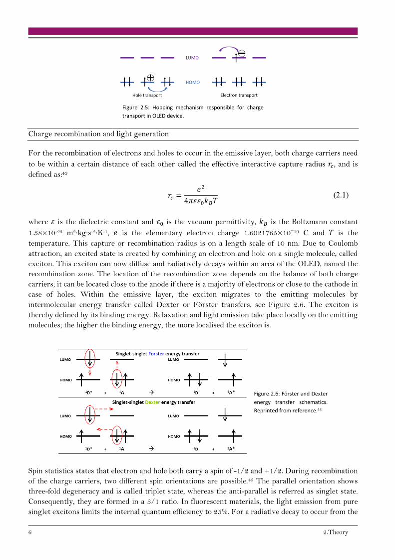
For the recombination of electrons and holes to occur in the emissive layer, both charge carriers need
to be within a certain distance of each other called the effective interactive capture radius 𝑟𝑐, and is
defined as:43
𝑟𝑐 =𝑒2
4𝜋𝜀𝜀0𝑘𝐵𝑇 (2.1)
where 𝜀 is the dielectric constant and 𝜀0 is the vacuum permittivity, 𝑘𝐵 is the Boltzmann constant
1.38×10⁻²³ m2∙kg∙s-2∙K-1, 𝑒 is the elementary electron charge 1.6021765×10⁻¹⁹ C and 𝑇 is the
temperature. This capture or recombination radius is on a length scale of 10 nm. Due to Coulomb
attraction, an excited state is created by combining an electron and hole on a single molecule, called
exciton. This exciton can now diffuse and radiatively decays within an area of the OLED, named the
recombination zone. The location of the recombination zone depends on the balance of both charge
carriers; it can be located close to the anode if there is a majority of electrons or close to the cathode in
case of holes. Within the emissive layer, the exciton migrates to the emitting molecules by
intermolecular energy transfer called Dexter or Förster transfers, see Figure 2.6. The exciton is
thereby defined by its binding energy. Relaxation and light emission take place locally on the emitting
molecules; the higher the binding energy, the more localised the exciton is.
Figure 2.6: Förster and Dexter
energy transfer schematics.
Reprinted from reference.44
Spin statistics states that electron and hole both carry a spin of -1/2 and +1/2. During recombination
of the charge carriers, two different spin orientations are possible.45 The parallel orientation shows
three-fold degeneracy and is called triplet state, whereas the anti-parallel is referred as singlet state.
Consequently, they are formed in a 3/1 ratio. In fluorescent materials, the light emission from pure
singlet excitons limits the internal quantum efficiency to 25%. For a radiative decay to occur from the
2.1. OLED introduction and architecture 7
triplet states (phosphorescence), intersystem crossing from triplet to singlet states is performed by
using materials containing heavy metals.46 These materials, also referred as triplet or phosphorescent
dopants, can harvest both singlet and triplet excitons and achieve a theoretical quantum efficiency of
100%, see Figure 2.7.46
Figure 2.7: Simplified energy diagram
representing different light emission
mechanisms. Fluorescence and
phosphorescence process are illustrated.
S0, S1 and T1 designate the singlet ground
state, the first singlet excited state and
the first triplet excited state, respectively.
2.1.1. Material deposition process
Electroluminescent materials can be divided in two types: small molecules2 and polymers47. The choice
of material is determining the deposition process of thin film organic layer. While small molecules can
be deposited by thermal vacuum evaporation and solution process, polymers can only be processed out
of solution (e.g., printing techniques4). Thin films of OLED materials in this work are prepared by
physical vapour deposition (PVD) and by inkjet printing. The details of the deposition techniques and
their application will be discussed below.
Physical vapour deposition process
Physical vapour deposition (PVD) is the most commonly used deposition process for OLEDs since its
introduction by Tang and VanSlyke in 1987.2 Under low pressure, pure materials are evaporated from
crucibles at elevated temperatures. Typically, OLED materials are evaporated at a pressure below 10-
7 mbar at relatively low temperature (< 300°C). The crucibles are resistively heated and controlled
using a thermocouple allowing regulation of the evaporation rate and the deposition rate. Thereby the
organic material is sublimed and the vapour propagates along the line-of-sight path towards a cooled
substrate, where it condenses to form a film. Using pure material under low vacuum makes PVD one
of the cleanest methods for material deposition. Cleanliness of the OLED fabrication method is critical
to achieve high device performance and long lifetime. PVD has several other advantages such as precise
control of thickness at the nanometre scale. It allows depositing complex multilayer stacks of a wide
range of materials with no interaction between subsequent layers. To control the lateral distribution,
the use of shadow masking is necessary and widely used for both lighting and display applications.
However, the alignment between mask and substrate is facing technological and physical limitations
when very fine patterning is requested, such as in high-resolution displays. In addition, the process of
evaporation under vacuum limits the panel size which must fit inside the chamber. In the recent years,
roll-to-roll thermal-evaporation was developed to enable the fabrication of large area and flexible
OLEDs.48

8 2.Theory
Solution process
In contrast, solution processes are compatible with large area substrates. For example, glass substrates
of 2.5 metres x 2.8 metres are coated by roll-to-roll processes allowing large scale material deposition
on both flexible and rigid substrates.10 The main advantage of solution processes is their cost
effectiveness. This is of high interest for OLED display costs to be competitive compared to LCDs and
plasma technologies. Solution processes can be used to deposit all organic layers, including small
molecules and polymer materials, with a very efficient material utilisation. Indeed, materials are
deposited only on the active areas of the substrate, unlike PVD which deposits material over the whole
substrate and the walls of the evaporation chamber. The “wet” deposition is compatible with a roll-to-
roll process on flexible substrates such as plastic films. Nonetheless, building complex multilayer
structures by soluble processes remains challenging. Each layer must be insoluble in the solvent used
to deposit the subsequent layer.49 This can be done by cross-linking the subjacent layer or by using
orthogonal solvents to process the next layer.50 Typically, soluble OLEDs fully processed from
solution are limited to three or four organic layers, whereas OLED processed from PVD can be
composed of more than ten layers.
Solution processes combine spin coating and printing. A low amount of ink is deposited onto a
substrate which spins to homogenise the thin film by centrifugal forces in the spin coating process.
Printing includes various processes, such as inkjet printing, screen printing, gravure, offset lithography
and flexography. For solution-processed OLED display fabrication, inkjet printing has the potential
to be the state-of-the-art technology for high R-G-B pixel definition.11-12 Patterning is used to set the
resolution of the overall display creating subpixel arrangements.51 Homogeneity is critical in both
inter- and intra- pixel film thickness, since inhomogeneous layer thickness results in poor colour
distribution, high voltage and lower device lifetime.
2.1.2. Soluble organic semiconductors
Both small molecules and polymers can be processed from solution as introduced in the previous
sections. The main difference between the two material classes is their weight distribution. Polymers
have a broad weight distribution and are referred as polydisperse materials, whereas small molecules
are monodisperse. Besides, the chain length of conjugated polymers can influence strongly the solution
viscosity which is an important criterion in solution processes. Both small molecules and polymer
materials can be used for hole injection, hole transport and/or emissive layers. In this work, the hole
injection and transport layers are made of polymers and the emissive layer of solution processable small
molecules.
Emissive materials: Small molecules
Small molecules were used in this work in the EML where holes and electrons recombine. The EML
can be either composed of one single material (undoped layer) or a mixture of materials (doped layer).
The non-doped configuration suffers from close packing in the solid state which leads to excimer
(excited dimer) and exciplex (excited complex) formation. Fluorescence quenching is hard to prevent
in the case of a single material in the EML.52 Nonetheless, aggregation of emitting molecules in the
solid state can be avoided in doped layers, i.e., a matrix composed of a small amount of emitting material
(usually 1-10%) diluted in a host material. This matrix configuration prevents luminescence quenching.

2.1. OLED introduction and architecture 9
Charge carriers are injected in the HOMO and the LUMO of the host material, followed by exciton
formation.
Combining emitters opens the possibility for a wide range of emissive colours, like white which can be
created with red, green and blue emitters,53 or yellow and blue emitters.54 Unlike polymers, small
molecules can be synthesised with very high purity, since they can be purified by recrystallisation and
sublimation.
Hole injection and hole transport materials: Polymers
The use of polymers in electronic applications has been made possible by Alan J. Heeger, Alan G.
MacDiarmid and Hideki Shirakawa in 1977 thanks to the discovery of iodine doped polyacetylene
exhibiting a high electrical conductivity.55
In this work, polymers are used for hole injection and hole transport. These materials must have a low-
lying HOMO comparable to the Fermi level of the anode to allow for efficient injection and transport
of holes into the HIL, the HTL and finally into the emissive layer (EML). In the case of the HTL, a
high-lying LUMO is needed to block negative charge carriers coming from the cathode. Attaching side
chains to the polymer helps tuning its solubility as well as its electronic and mechanical properties.
Commonly used hole transport materials are depicted in Figure 2.8.56
Figure 2.8: Chemical structure of common hole transporting materials.
PTAA stands for poly[bis(4-phenyl)(2,4,6-trimethylphenyl)]amine and is an excellent hole transport
and electron blocking material.57 Polyaniline is written as PANi and TFB corresponds to poly(9,9-
10 2.Theory
dioctylfluorene-alt-N-(4-sec-butylphenyl)-diphenylamine), a common hole transport polymer.58-59
Polycarbazole shows strong interchain charge transport properties through hopping.60
Polymer materials are composed of a succession of monomers which are classified depending on their
functionality. Three monomer types exist: amine, backbone, and cross-linker units. The amine
monomer controls the HOMO level and the charge transport properties. The backbone is responsible
for the rigidity of the material. Side chains attached to the backbone help for a good material solubility.
Cross-linking units added to the polymer chain enhance mechanical, thermal and chemical resistance
properties after the cross-linking reaction has been successfully performed. The cross-linking
chemistry is discussed in the following section.
Cross-linker units
Cross-linking units can be thermally or photochemically activated, like styrene and acrylate moieties,
respectively.61 The cross-linking process leads to the creation of a covalent bond between two or more
molecules. It forms a network encompassing the entire system. A fully cross-linked polymer can only
be swollen in a solvent, it cannot be dissolved. These cross-linking units are widely used for solution
processable OLED materials.61 The challenge is the degree of cross-linking, which characterises how
complete the cross-linking reaction succeeded. Indeed, remaining unreacted cross-linking units can
significantly reduce device performance and lifetime.
It exists a wide range of cross-linker units used for OLED devices.61 Siloxane was reported for the first
time to be used for cross-linking in an OLED device in 1999.25 Despite strong and stable resulting
bonds, water and alcohols were found in the film and behave as impurities. Styrene moieties can be
attached to small molecules and polymers to perform cross-linking by thermal activation.
Consequently, the material to which the styrene is attached must be stable at its reaction temperature.
Besides these popular cross-linker units, trifluorovinylether, benzocyclobutene, oxetane, cinnamate
and chalcone, are also used for cross-linking in OLED devices.
2.2. Inkjet printing of thin films
Inkjet printing is the method of choice for various organic electronic applications such as OLEDs,4
OPVs62 and OFETs.63 As introduced in Chapter 2.1.1, the main reason is that inkjet printing offers
high precision control over numerous substrates without the need of shadow masking. This non-
contact deposition technique is one of the most cost-efficient ways of producing complex pattern thanks
to its efficient use of materials.
2.2.1. Instrumentation and operation mode
Continuous inkjet printer64 and drop-on-demand (DoD) inkjet printer65 are the two commercial types
of inkjet printers. Commercial marking and coding of products and packages are mainly produced by
continuous printers, whereas drop-on-demand inkjet printers are used for organic electronics
applications.66
A continuous inkjet printer is composed of a fluid reservoir which supplies the ink, one or more nozzles
and electrostatically charged plates. The droplet is ejected from the nozzle(s) and the charged plates
2.2. Inkjet printing of thin films 11
deflect the droplet so that it reaches the desired position on the substrate. A cup is used to collect the
droplets that should not be printed on the substrate.
In opposite, DoD inkjet printer consists of a low fluid impedance nozzle67 and a thermal or piezoelectric
actuator which generates a pressure pulse in the fluid to push a droplet out of the nozzle. The landing
of the droplet is controlled by a highly precise mechanical system that moves the print-head in two
dimensions and the substrate holder in one dimension leading to the positions of the desired pattern,
see Figure 2.9c. The droplet ejection process is displayed in Figure 2.9a from a continuous inkjet
printer and in Figure 2.9b from a DoD printer. The display industry favours DoD inkjet printers as
being able to create complex pixelated structures with the dimensions and precision needed for state
of the art OLED performance.68
Figure 2.9: Schematics of (a) continuous, (b) Drop-on-Demand printing. Droplet ejection process from the print-head
reprinted from reference.69 (c) Schematics of mechanical system control of the substrate holder and the print-head in one
and two dimensions, respectively.
2.2.2. Print-heads
As introduced in Chapter 2.2.1., DoD inkjet printers can use thermal or piezoelectric inkjet print-heads.
The extreme heat needed to form a droplet from a thermal print-head is unfavourable for its use in
printed electronics. Therefore, piezoelectric inkjet print-heads are the system of choice. A schematic
diagram of a piezoelectric inkjet print-head is illustrated in Figure 2.10.
Figure 2.10: Schematic
diagram of a piezoelectric
inkjet print-head. Reprinted
from reference.66
(a) Continuous (b) Drop-on-Demand (c) Mechanical system

12 2.Theory
In piezoelectric inkjet print-heads, the piezoelectric material converts electrical energy into mechanical
deformation of the ink chamber resulting in a pressure change in the chamber. This leads to the
formation and ejection of a drop from the nozzle. Different modes of deformation are possible and
represented in Figure 2.11.
Figure 2.11: Different piezoelectric
element arrangement in drop-on-
demand inkjet print-heads.
Reprinted from reference.70
The ink reservoir is connected to the capillary cavity by an open end. A pressure line is also linked to
the ink supply in order to aspirate and flush ink through the print-head for maintenance. The capillary
cavity is enveloped by a piezoelectric actuator running at eigenfrequency. The print-head ends with a
nozzle aperture from where droplets are generated from the ink. The diameter of the nozzle is much
smaller than the cavity, thus it is called a closed end. To avoid dripping of ink from the nozzle, a slight
under-pressure is applied. A droplet is formed by applying a generally square shaped waveform with
double-peak. For the Dimatix print-head DMC, the eigenfrequency is 12 kHz. To produce a 10 pL
droplet from DMC, the nozzle diameter is of 21.5 µm and the applied under-pressure is 2 mbar
compared to the surrounding pressure. The Q-class print-head requires an under-pressure of 25 mbar.
When a positive pressure wave approaches the nozzle, a droplet is generated if the amplitude and
velocity of the wave are large enough. The surface energy needed to form a droplet at the nozzle plate
must be exceeded by the amount of kinetic energy transferred outwards.71 In addition, due to the
decelerating action of ambient air, the velocity of a droplet necessitates to be several metres per second
so that the droplet can meet the targeted landing position.72 Generally, piezoelectric print-heads can
process ink with a viscosity lower than 20 mPa∙s and surface tensions between 20 mN∙m-1 and 70
mN∙m-1.
2.2.3. Challenges
Despite the advantages of inkjet printing techniques presented in Chapter 2.1.1, ink jetting through
the nozzle(s) and film formation are challenging steps of the process.
Droplet formation
In the case of a piezoelectric inkjet print-head, a droplet is formed by the piezoelectric crystal excited
by an electrical pulse, called waveform,73 which can be tuned accordingly to the ink viscosity,
2.2. Inkjet printing of thin films 13
concentration and surface tension. Changes in the waveform directly impact the droplet velocity which
is targeted at 4-5 m∙s-1. The droplet volume is not only influenced by the nozzle diameter, but also
strongly by the waveform66 and printer type. The volume can vary between 1 pL to 20 pL, it should
be chosen in line with the pattern resolution wanted, or rather the display resolution (individual pixel
size). In this work, droplet of 10 pL were printed. Printing in a pixelated substrate requires a stable
droplet, which includes reproducible droplet formation at high frequency and a reproducible droplet
landing. This can be achieved when the droplet forms an angle of less than 1° with the line
perpendicular to the substrate.
The droplet formation through a nozzle typically shows a non-Newtonian fluid behaviour. After the
pulse ejecting the fluid out of the nozzle, the droplet remains attached to the nozzle by a filament.
Then, a pinch point is formed right above the droplet which breaks the connection to the nozzle and a
filament appears. The filament undergoes thinning and either retracts back into the droplet or it can
eventually break up into satellite droplets of much smaller volume.66 Satellite droplets and long
filament can create misprints in the desired patterning resulting in inhomogeneous printing,
problematic especially for functional printing. No droplet formation might occur due to mismatch of
fluid surface tension and the print-head material. Elastic stresses are associated to the behaviour of
polymer solution, as suggested by Schubert et al.74 This behaviour stops operating for very viscous
solution of high concentration, or made with high molecular weight materials. In this case, capillary
forces cannot break the filament and the droplet bounces back to the nozzle plate. The different stages
of droplet formation are depicted in Figure 2.12.
Figure 2.12: High speed photographic images of droplet
formation from a DoD printer. Through time, the droplet is
attached to the print-head by a ligament, which then breaks into
satellite. Finally, they retract to the leading droplet. Reprinted
from reference.75
The printability of conjugated polymers can also be affected by inter-chain interaction and thus impacts
film morphology. Solvent polarity, its aromatic nature and polymer concentration are important
parameters influencing the degree of inter-chain interactions.76
Large area film formation
The inkjet printing technique using high boiling point solvents, exhibit a great challenge concerning
film formation. In the frame of this work, large area squares (4 cm²) must be printed in order to pursue
thin film characterisation techniques. In order to reach a flat and smooth film, the first criterion is that
every droplet printed on a substrate must merge to the neighbouring one without a big overlap. The
droplet spacing should be smaller than the critical value but too small droplet spacing bring film
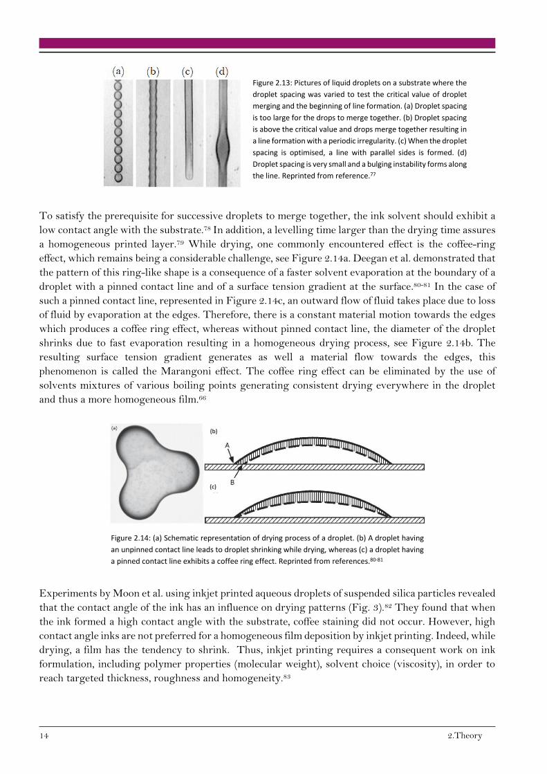
instabilities.76 The impact of the droplet spacing on line formation is depicted Figure 2.13, where the
droplet spacing decreases from (a) to (d). The critical value is reached between the droplet spacing
displayed in (a) and (b), where merging occurred.
14 2.Theory
Figure 2.13: Pictures of liquid droplets on a substrate where the
droplet spacing was varied to test the critical value of droplet
merging and the beginning of line formation. (a) Droplet spacing
is too large for the drops to merge together. (b) Droplet spacing
is above the critical value and drops merge together resulting in
a line formation with a periodic irregularity. (c) When the droplet
spacing is optimised, a line with parallel sides is formed. (d)
Droplet spacing is very small and a bulging instability forms along
the line. Reprinted from reference.77
To satisfy the prerequisite for successive droplets to merge together, the ink solvent should exhibit a
low contact angle with the substrate.78 In addition, a levelling time larger than the drying time assures
a homogeneous printed layer.79 While drying, one commonly encountered effect is the coffee-ring
effect, which remains being a considerable challenge, see Figure 2.14a. Deegan et al. demonstrated that
the pattern of this ring-like shape is a consequence of a faster solvent evaporation at the boundary of a
droplet with a pinned contact line and of a surface tension gradient at the surface.80-81 In the case of
such a pinned contact line, represented in Figure 2.14c, an outward flow of fluid takes place due to loss
of fluid by evaporation at the edges. Therefore, there is a constant material motion towards the edges
which produces a coffee ring effect, whereas without pinned contact line, the diameter of the droplet
shrinks due to fast evaporation resulting in a homogeneous drying process, see Figure 2.14b. The
resulting surface tension gradient generates as well a material flow towards the edges, this
phenomenon is called the Marangoni effect. The coffee ring effect can be eliminated by the use of
solvents mixtures of various boiling points generating consistent drying everywhere in the droplet
and thus a more homogeneous film.66
Figure 2.14: (a) Schematic representation of drying process of a droplet. (b) A droplet having
an unpinned contact line leads to droplet shrinking while drying, whereas (c) a droplet having
a pinned contact line exhibits a coffee ring effect. Reprinted from references.80-81
Experiments by Moon et al. using inkjet printed aqueous droplets of suspended silica particles revealed
that the contact angle of the ink has an influence on drying patterns (Fig. 3).82 They found that when
the ink formed a high contact angle with the substrate, coffee staining did not occur. However, high
contact angle inks are not preferred for a homogeneous film deposition by inkjet printing. Indeed, while
drying, a film has the tendency to shrink. Thus, inkjet printing requires a consequent work on ink
formulation, including polymer properties (molecular weight), solvent choice (viscosity), in order to
reach targeted thickness, roughness and homogeneity.83
(c)
(b)

2.3. IJP inks: Polymer solutions 15
2.3. IJP inks: Polymer solutions
In this work, the focus is set on polymer solutions, which can be seen as a mixture of long
macromolecular chains and small molecules of solvents.84 Due to diverse conformations that the
flexible chains may take, special methods must be taken into account. In order to study the physical-
chemical properties of polymers in solution, the mixture must be in the dilute regime where no
interaction between the chains is taking place or is reduced to a minimum. In dilute solutions,
individual macromolecules properties are studied, whereas in concentrated solutions, the chains are
entangled and consequently the contribution of a single macromolecule cannot be evaluated.
2.3.1. Polymer solubility profile
Complete polymer dissolution can occur instantaneously but can also last up to days or weeks.
Billmeyer Jr. identified polymer dissolution following two steps.85 First the polymer swells, then
second the dissolution itself takes place. The polymer coil, together with solvent molecules attached,
adopts a thermodynamic arrangement in solution, as displayed in Figure 2.15.
Figure 2.15: Schematic representation of the dissolution process for
polymer molecules. In a theta solvent, the polymer coil adopts a spherical
form.
The rule of thumb stating “like dissolves like” gives a good appreciation of polymer solubility.86
(Non)Polar solvents dissolve (non)polar solutes. Yet, polymer dissolution depends on many other
parameters, such as molecular weight, branching, degree of cross-linking and crystallinity. An increase
of molecular weight, at constant temperature, leads to a decrease in polymer solubility. The same
behaviour is observed as the degree of cross-linking increases. Indeed, the cross-linked polymer hinders
interaction between polymer chains and solvent molecules, rendering them insoluble and resulting in
a swollen gel. When the solubility of a polymer cannot be directly determined by standard
measurements, an indirect method allows understanding the solubility range of a polymer and the ink
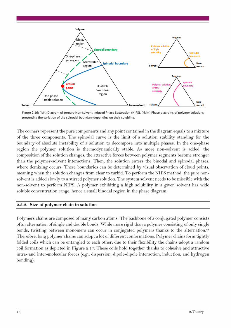
stability. The Non-solvent Induced Phase Separation (NIPS) is a well-established technique also
known as Loeb-Sourirajan method, as well as immersion precipitation and Diffusion Induced Phase
Separation (DIPS).87 To perform this method, three components are needed: a polymer, a solvent and
a non-solvent for the investigated polymer. A typical ternary NIPS, illustrated in Figure 2.16, was
used to describe an ink stability, i.e., the capability of an ink to remain a single-phase system while non-
solvent is added.
16 2.Theory
Figure 2.16: (left) Diagram of ternary Non-solvent Induced Phase Separation (NIPS). (right) Phase diagrams of polymer solutions
presenting the variation of the spinodal boundary depending on their solubility.
The corners represent the pure components and any point contained in the diagram equals to a mixture
of the three components. The spinodal curve is the limit of a solution stability standing for the
boundary of absolute instability of a solution to decompose into multiple phases. In the one-phase
region the polymer solution is thermodynamically stable. As more non-solvent is added, the
composition of the solution changes, the attractive forces between polymer segments become stronger
than the polymer-solvent interactions. Then, the solution enters the binodal and spinodal phases,
where demixing occurs. These boundaries can be determined by visual observation of cloud points,
meaning when the solution changes from clear to turbid. To perform the NIPS method, the pure non-
solvent is added slowly to a stirred polymer solution. The system solvent needs to be miscible with the
non-solvent to perform NIPS. A polymer exhibiting a high solubility in a given solvent has wide
soluble concentration range, hence a small binodal region in the phase diagram.
2.3.2. Size of polymer chain in solution
Polymers chains are composed of many carbon atoms. The backbone of a conjugated polymer consists
of an alternation of single and double bonds. While more rigid than a polymer consisting of only single
bonds, twisting between monomers can occur in conjugated polymers thanks to the alternation.88
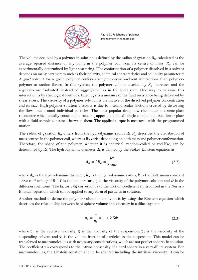
Therefore, long polymer chains can adopt a lot of different conformations. Polymer chains form tightly
folded coils which can be entangled to each other; due to their flexibility the chains adopt a random
coil formation as depicted in Figure 2.17. These coils hold together thanks to cohesive and attractive
intra- and inter-molecular forces (e.g., dispersion, dipole-dipole interaction, induction, and hydrogen
bonding).
2.3. IJP inks: Polymer solutions 17
Figure 2.17: Scheme of polymer
arrangement in random coil.
The volume occupied by a polymer in solution is defined by the radius of gyration Rg, calculated as the
average squared distance of any point in the polymer coil from its centre of mass. 𝑅𝑔 can be
experimentally determined by light scattering. The conformation of a polymer dissolved in a solvent
depends on many parameters such as their polarity, chemical characteristics and solubility parameter.89
A good solvent for a given polymer confers stronger polymer-solvent interactions than polymer-
polymer attraction forces. In this system, the polymer volume marked by 𝑅𝑔 increases and the
segments are “solvated” instead of “aggregated” as in the solid state. One way to measure this
interaction is by rheological methods. Rheology is a measure of the fluid resistance being deformed by
shear stress. The viscosity of a polymer solution is distinctive of the dissolved polymer concentration
and its size. High polymer solution viscosity is due to intermolecular frictions created by distorting
the flow lines around individual particles. The most popular drag flow rheometer is a cone-plate
rheometer which usually consists of a rotating upper plate (small-angle cone) and a fixed lower plate
with a fluid sample contained between them. The applied torque is measured with the programmed
motion.
The radius of gyration 𝑅𝑔 differs from the hydrodynamic radius Rh. 𝑅𝑔 describes the distribution of
mass centres in the polymer coil, whereas Rh varies depending on both mass and polymer conformation.
Therefore, the shape of the polymer, whether it is spherical, random-coiled or rod-like, can be
determined by Rh. The hydrodynamic diameter 𝑑ℎ is defined by the Stokes-Einstein equation as:
where 𝑑ℎ is the hydrodynamic diameter, 𝑅ℎ is the hydrodynamic radius, 𝑘 is the Boltzmann constant
1.38×10⁻²³ m2∙kg∙s-2∙K-1, 𝑇 is the temperature, 𝜂 is the viscosity of the polymer solution and 𝐷 is the
diffusion coefficient. The factor 3𝜋𝜂 corresponds to the friction coefficient ζ introduced in the Nernst-
Einstein equation, which can be applied to any form of particles in solution.
Another method to define the polymer volume in a solvent is by using the Einstein equation which
describes the relationship between hard sphere volume and viscosity in a dilute system:
𝜂𝑟 =𝜂
𝜂𝑠= 1 + 2.5𝛷 (2.3)
where 𝜂𝑟 is the relative viscosity, η is the viscosity of the suspension, 𝜂𝑠 is the viscosity of the
suspending solvent and 𝛷 is the volume fraction of particles in the suspension. This model can be
transferred to macromolecules with necessary considerations, which are not perfect spheres in solution.
The coefficient 2.5 corresponds to the intrinsic viscosity of a hard sphere in a very dilute system. For
macromolecules, the Einstein equation should be adapted including the intrinsic viscosity. It can be
𝑑ℎ = 2𝑅ℎ =𝑘𝑇
3𝜋𝜂𝐷 (2.2)
18 2.Theory
inferred that for a polymer dissolved in a poor solvent, conferring stronger polymer-polymer attraction
forces than polymer-solvent interactions, the resulting viscosity of the solution should be small. Thus,
rheology is a tool to record solvent interaction with a given polymer.
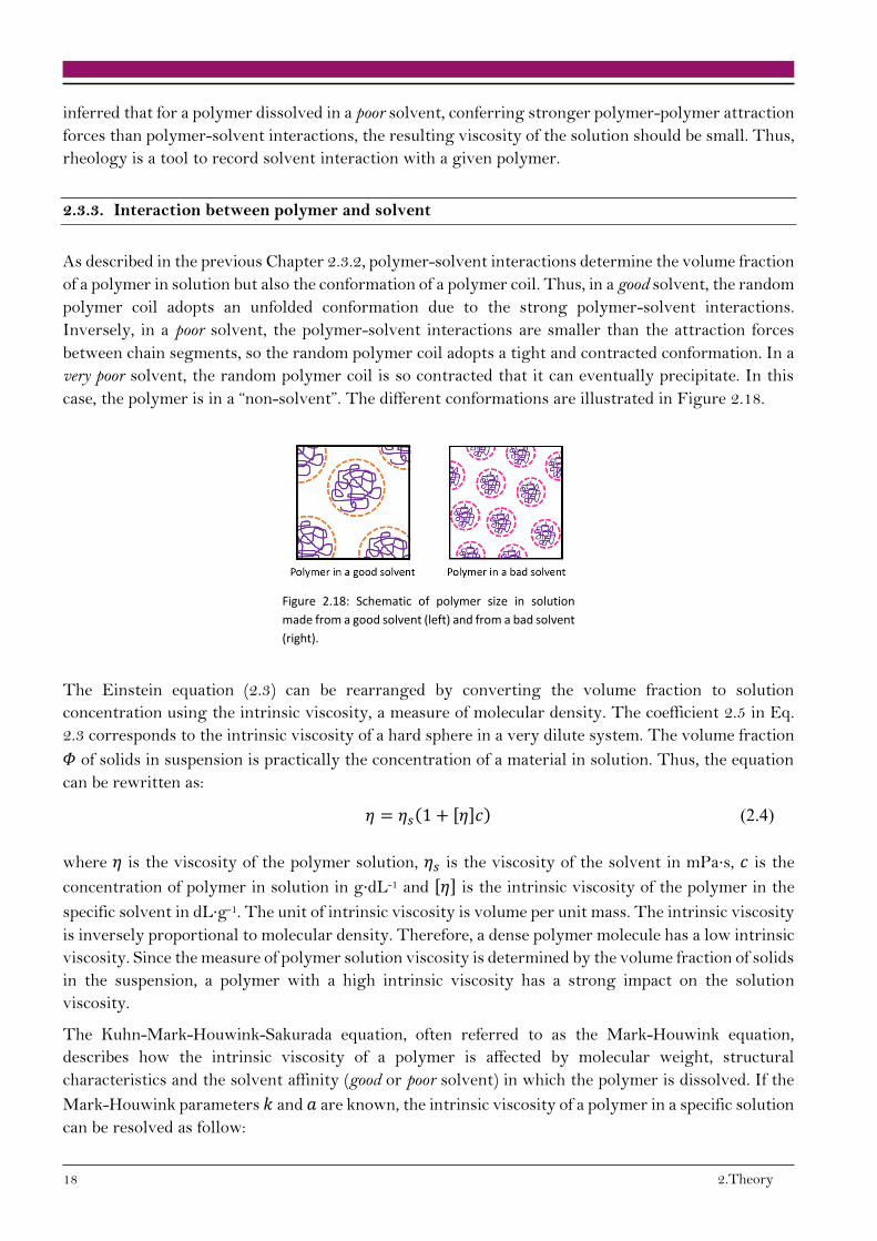
2.3.3. Interaction between polymer and solvent
As described in the previous Chapter 2.3.2, polymer-solvent interactions determine the volume fraction
of a polymer in solution but also the conformation of a polymer coil. Thus, in a good solvent, the random
polymer coil adopts an unfolded conformation due to the strong polymer-solvent interactions.
Inversely, in a poor solvent, the polymer-solvent interactions are smaller than the attraction forces
between chain segments, so the random polymer coil adopts a tight and contracted conformation. In a
very poor solvent, the random polymer coil is so contracted that it can eventually precipitate. In this
case, the polymer is in a “non-solvent”. The different conformations are illustrated in Figure 2.18.
Figure 2.18: Schematic of polymer size in solution
made from a good solvent (left) and from a bad solvent
(right).
The Einstein equation (2.3) can be rearranged by converting the volume fraction to solution
concentration using the intrinsic viscosity, a measure of molecular density. The coefficient 2.5 in Eq.
2.3 corresponds to the intrinsic viscosity of a hard sphere in a very dilute system. The volume fraction
𝛷 of solids in suspension is practically the concentration of a material in solution. Thus, the equation
can be rewritten as:
𝜂 = 𝜂𝑠(1 + [𝜂]𝑐) (2.4)
where 𝜂 is the viscosity of the polymer solution, 𝜂𝑠 is the viscosity of the solvent in mPa∙s, 𝑐 is the
concentration of polymer in solution in g∙dL-1 and [𝜂] is the intrinsic viscosity of the polymer in the
specific solvent in dL∙g-1. The unit of intrinsic viscosity is volume per unit mass. The intrinsic viscosity
is inversely proportional to molecular density. Therefore, a dense polymer molecule has a low intrinsic
viscosity. Since the measure of polymer solution viscosity is determined by the volume fraction of solids
in the suspension, a polymer with a high intrinsic viscosity has a strong impact on the solution
viscosity.
The Kuhn-Mark-Houwink-Sakurada equation, often referred to as the Mark-Houwink equation,
describes how the intrinsic viscosity of a polymer is affected by molecular weight, structural
characteristics and the solvent affinity (good or poor solvent) in which the polymer is dissolved. If the
Mark-Houwink parameters 𝑘 and 𝑎 are known, the intrinsic viscosity of a polymer in a specific solution
can be resolved as follow:

2.3. IJP inks: Polymer solutions 19
where [𝜂] is the intrinsic viscosity of the polymer in the specific solvent, 𝑀𝑤 is the molecular weight,
and 𝑘 and 𝑎 are the MH parameters. The intrinsic viscosity can also be determined by measuring the
viscosity of the polymer solution over a range of concentrations and fitting the Huggins or Kraemer
equations.90 These empirical observations will be detailed in Chapter 4.
[𝜂] = 𝑘 · 𝑀𝑤𝑎 (2.5)

3.1. Materials 21
3. Investigated System and Methods
The hole transport material under investigation was processed from five different inkjet printing
solvents. The interaction between the polymer and each solvent was characterised by various
techniques in solution. The resulting inkjet printed polymer film properties were determined to
understand their stability against solvent exposure. Finally, OLED devices were built to evaluate the
impact of the HTL ink solvent on their electrical properties.
3.1. Materials
In this work, two classes of organic semiconductors were used. The HIL consists of a mixture of a
polymer and small molecules. For the HTL, a polymer is employed. A blend of small molecules
composes the EML where the molecules either emit light or transport charge carriers. The HIL, HTL
and EML were processed from solution. The ETL and the EIL consist of small molecules that were
deposited by PVD. Unlike polymers whose molecular weight is over 20,000 g∙mol-1, small molecules
exhibit a molecular weight of up to 3000 g∙mol-1 which enables them to be either evaporated under
high vacuum or processed from solution.
3.1.1. Hole transport materials
X-Po, a Merck cross-linkable hole transport material, described in the patent WO2013/156130 A1 as
polymer Po2,91 is the main investigated polymer in this thesis. The molecular weight of the X-Po batch
is 82 kg∙mol-1. The hole transport layer material consists of a random co-polymer, whose monomers
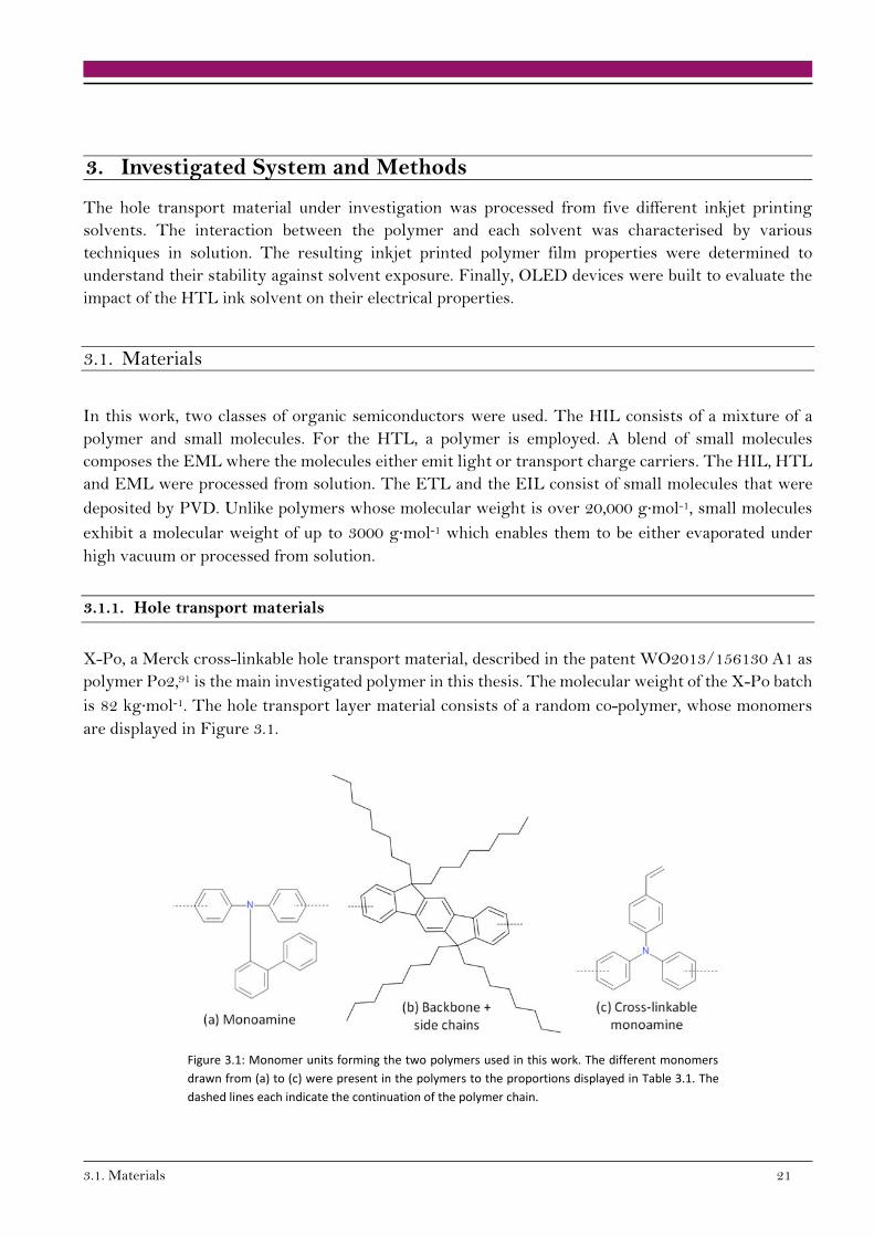
are displayed in Figure 3.1.
Figure 3.1: Monomer units forming the two polymers used in this work. The different monomers
drawn from (a) to (c) were present in the polymers to the proportions displayed in Table 3.1. The
dashed lines each indicate the continuation of the polymer chain.

22 3.Investigated System and Methods
Po, the non-cross-linkable version of X-Po, was also studied. X-Po and Po differ in the presence of a
cross-linkable unit, whose ratio between the different monomer units is reported in Table 3.1. These
were the following monomers: (a) a triaryl amine (TAA) unit, (b) the backbone where side chains are
attached which have the purpose to increase the chain solubility, and (c) a TAA hosting a thermally
cross-linkable group. The cross-linkable group consisted of a styrene-type cross-linker.
Table 3.1: Monomer units contained in X-Po and Po.
Polymer (a) Monoamine (b) Backbone +
side chains
(c) Cross-linkable
monoamine
X-Po 40% 50% 10%
Po 50% 50% 0%
Figure 3.2 displays the absorption spectra of the two hole transport materials measured from spin
coated films processed from toluene. The absorption edge is at 436 nm, which results in a calculated
energy gap 𝐸𝑔 =ℎ𝑐
𝜆 of 2.84 eV for both polymers. The HOMO values were measured in films by
photoelectron spectroscopy in air using a Riken AC3. The LUMO values were estimated by adding
the calculated energy gap to the Riken HOMO level. The HOMO and LUMO levels of both polymers
are listed in
Table 3.2.
Figure 3.2: Absorption spectra
of the hole transport materials
measured in spin coated films
processed from toluene.
Table 3.2: HOMO and LUMO levels of X-Po and Po. HOMO values of the hole transport materials
measured by photoelectron spectroscopy (Riken) and the calculated LUMO of these materials.
Polymer
material
HOMO
(Riken)
LUMO
(Riken + Abs.) Eg = hc/λ
X-Po -5.61 eV -2.77 eV 1240/436 = 2.84 eV
Po -5.58 eV -2.74 eV 1240/436 = 2.84 eV
3.1.2. Inkjet printing solvents
To process organic semiconductors from solution, and more specifically for inkjet printing, the chosen
solvents must obey specific criteria. Their surface tension should allow for the formation of well-shaped
droplets after ejection from the print-head, see Chapter 2.2.3, and they should wet the substrate. In
addition, the solvents need a low viscosity, especially taking into account that linear polymers show a
3.1. Materials 23
strong increase in viscosity with concentration. Further, solvents with a high boiling point were chosen
to avoid clogging of the 21.5 µm diameter nozzles of the print-head. At the same time, the processing
of organic semiconductors from solution requires that the materials have good solubility in the solvents
and that the solvent should be chemically inert to the materials dissolved therein.
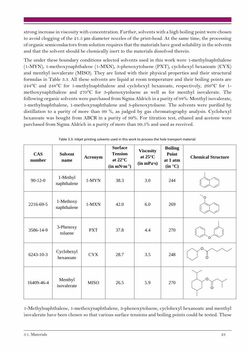
The under these boundary conditions selected solvents used in this work were 1-methylnaphthalene
(1-MYN), 1-methoxynaphthalene (1-MXN), 3-phenoxytoluene (PXT), cyclohexyl hexanoate (CYX)
and menthyl isovalerate (MISO). They are listed with their physical properties and their structural
formulas in Table 3.3. All these solvents are liquid at room temperature and their boiling points are
244°C and 248°C for 1-methylnaphthalene and cyclohexyl hexanoate, respectively, 269°C for 1-
methoxynaphthalene and 270°C for 3-phenoxytoluene as well as for menthyl isovalerate. The
following organic solvents were purchased from Sigma Aldrich in a purity of 98%: Menthyl isovalerate,
1-methylnaphthalene, 1-methoxynaphthalene and 3-phenoxytoluene. The solvents were purified by
distillation to a purity of more than 99 %, as judged by gas chromatography analysis. Cyclohexyl
hexanoate was bought from ABCR in a purity of 99%. For titration test, ethanol and acetone were
purchased from Sigma Aldrich in a purity of more than 99.5% and used as received.
Table 3.3: Inkjet printing solvents used in this work to process the hole transport material.
CAS
number
Solvent
name Acronym
Surface
Tension
at 22°C
(in mN∙m-1)
Viscosity
at 25°C
(in mPa∙s)
Boiling
Point
at 1 atm
(in °C)
Chemical Structure
90-12-0 1-Methyl
naphthalene 1-MYN 38.3 3.0 244
2216-69-5 1-Methoxy
naphthalene 1-MXN 42.0 6.0 269
3586-14-9 3-Phenoxy
toluene PXT 37.8 4.4 270
6243-10-3 Cyclohexyl
hexanoate CYX 28.7 3.5 248
16409-46-4 Menthyl
isovalerate MISO 26.5 5.9 270
1-Methylnaphthalene, 1-methoxynaphthalene, 3-phenoxytoluene, cyclohexyl hexanoate and menthyl
isovalerate have been chosen so that various surface tensions and boiling points could be tested. These
O
O
O
O
O
O
24 3.Investigated System and Methods
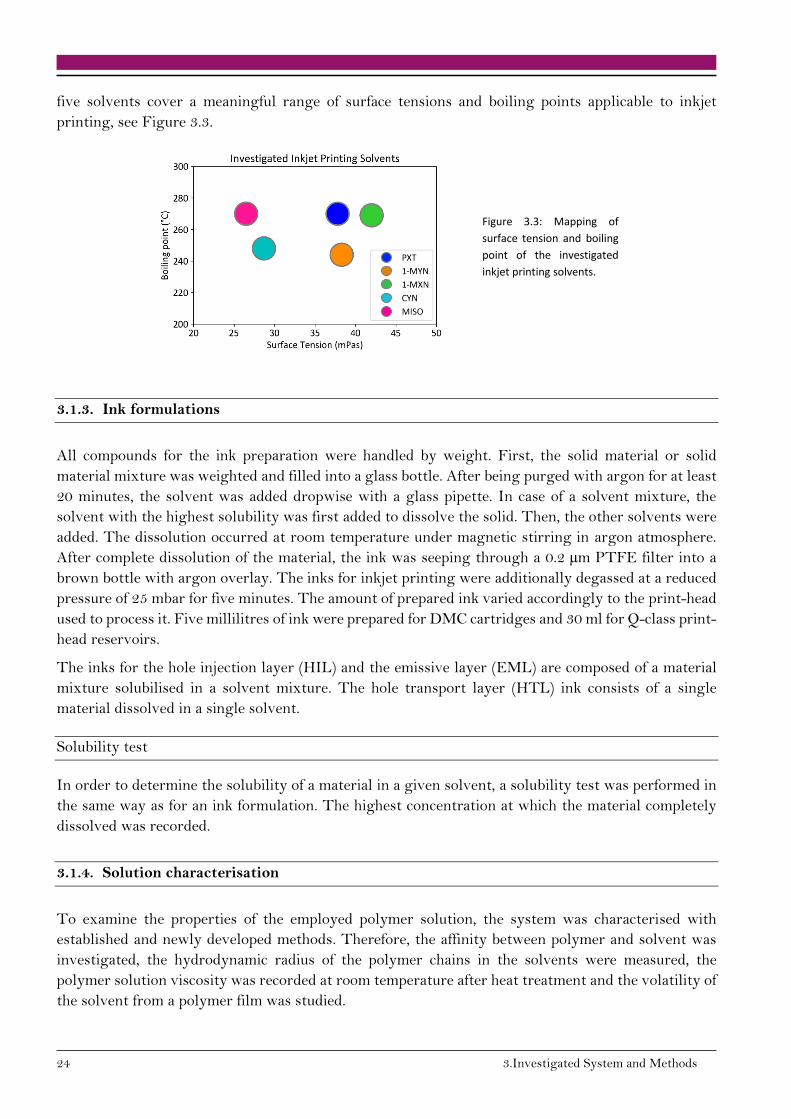
five solvents cover a meaningful range of surface tensions and boiling points applicable to inkjet
printing, see Figure 3.3.
Figure 3.3: Mapping of
surface tension and boiling
point of the investigated
inkjet printing solvents.
3.1.3. Ink formulations
All compounds for the ink preparation were handled by weight. First, the solid material or solid
material mixture was weighted and filled into a glass bottle. After being purged with argon for at least
20 minutes, the solvent was added dropwise with a glass pipette. In case of a solvent mixture, the
solvent with the highest solubility was first added to dissolve the solid. Then, the other solvents were
added. The dissolution occurred at room temperature under magnetic stirring in argon atmosphere.
After complete dissolution of the material, the ink was seeping through a 0.2 µm PTFE filter into a
brown bottle with argon overlay. The inks for inkjet printing were additionally degassed at a reduced
pressure of 25 mbar for five minutes. The amount of prepared ink varied accordingly to the print-head
used to process it. Five millilitres of ink were prepared for DMC cartridges and 30 ml for Q-class print-
head reservoirs.
The inks for the hole injection layer (HIL) and the emissive layer (EML) are composed of a material
mixture solubilised in a solvent mixture. The hole transport layer (HTL) ink consists of a single
material dissolved in a single solvent.
Solubility test
In order to determine the solubility of a material in a given solvent, a solubility test was performed in
the same way as for an ink formulation. The highest concentration at which the material completely
dissolved was recorded.
3.1.4. Solution characterisation
To examine the properties of the employed polymer solution, the system was characterised with
established and newly developed methods. Therefore, the affinity between polymer and solvent was
investigated, the hydrodynamic radius of the polymer chains in the solvents were measured, the
polymer solution viscosity was recorded at room temperature after heat treatment and the volatility of
the solvent from a polymer film was studied.

3.1. Materials 25
Polymer-solvent affinity
Polymer-solvent affinity was determined using a precipitation/demixing test based on the NIPS
technique, introduced in Chapter 2.3.3.87 Ethanol was considered to be a poor solvent for X-Po. It was
used to precipitate the polymer X-Po from solution of each solvent utilised in the present study. A 1.5
mL solution of polymer X-Po was prepared at 30 g∙L-1 with each solvent in glass bottles. The high
concentration of 30 g∙L-1 facilitated the visualisation of the precipitation onset. Ethanol was added to
the mixture dropwise under magnetic stirring. The beginning of precipitation was determined visually
as the moment the solution turned turbid. The amount of ethanol added at which the mixture started
to precipitate was recorded. The more ethanol was needed to start the precipitation of the polymer
solution, the stronger was the interaction between polymer and solvent. Such strong interaction was
characteristic of a good solvent92 for X-Po.
Size of particles in solution: Hydrodynamic radius Rh
The size and organisation of the polymer in solution was investigated by light scattering
methodologies.93 “Classical light scattering”, also called “static” or “Rayleigh” scattering is employed
to directly measure the weight-average molecular weight of a polymer (Mw). “Dynamic light
scattering” (DLS), also known as “photon correlation spectroscopy” (PCS) or “quasi-elastic light
scattering” (QELS) can be used to measure the rate of diffusion of polymer particles in solution. This
diffused light collected from the Brownian motion of polymer particles is sensitive to the presence of
very small amounts of aggregated polymer particles and can deliver the polymer size distribution over
a large range of masses. Thereby small particles diffuse rapidly, whereas large particles diffuse slowly.
Additionally, the speed of diffusion also depends on the viscosity of the dispersant.
The size distribution obtained by DLS is representative for the light intensity that is scattered by
particles in suspension of diverse diameters. If the sample is polymodal (more than one discrete peak)
and polydisperse (broad peak), it is recommended to use the Mie theory to convert the intensity
distribution to a volume distribution by considering the refractive index of the polymer solution. The
volume representation of a polymodal and polydisperse sample provides a more real picture of the
proportions of the particle sizes in solution.94 DLS measurements were carried out with disposable
plastic cuvettes at 25°C. In order to utilise the volume representation, the viscosity of the solution had
to be introduced to the software.
Viscosity
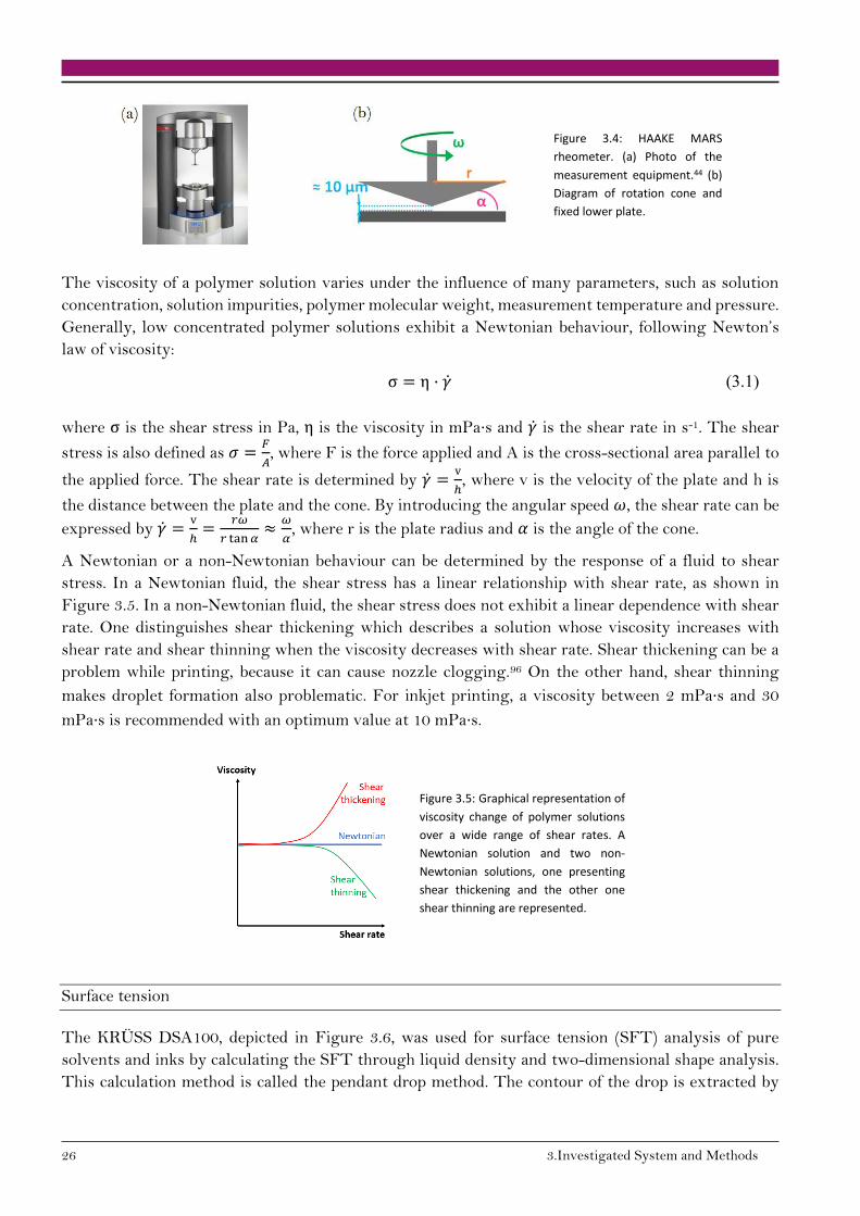
Viscosity measurements were carried out using a HAAKE MARS rheometer (Modular Advanced
Rheometer System), see Figure 3.4. The viscosity was measured in a cone-plate geometry over a range
of shear rates from 0.5 to 1000 s-1 with 20 logarithmically spaced steps at a constant temperature of
25°C. The temperature was controlled by a Peltier plate with 0.2°C accuracy. A small fluid sample (1.3
mL) was placed with an Eppendorf pipette in the space between a fixed lower plate of radius 𝑟 (TMP60)
and a rotating cone of the same radius with a very small angle 𝛼 (C60/1°). The sample must have a
free spherical shaped surface at the outer edge to insure an accurate measurement.95
26 3.Investigated System and Methods
Figure 3.4: HAAKE MARS
rheometer. (a) Photo of the
measurement equipment.44 (b)
Diagram of rotation cone and
fixed lower plate.
The viscosity of a polymer solution varies under the influence of many parameters, such as solution
concentration, solution impurities, polymer molecular weight, measurement temperature and pressure.
Generally, low concentrated polymer solutions exhibit a Newtonian behaviour, following Newton’s
law of viscosity:
σ = η · �̇� (3.1)
where σ is the shear stress in Pa, η is the viscosity in mPa∙s and �̇� is the shear rate in s-1. The shear
stress is also defined as 𝜎 =𝐹
𝐴, where F is the force applied and A is the cross-sectional area parallel to
the applied force. The shear rate is determined by �̇� =v
ℎ, where v is the velocity of the plate and h is
the distance between the plate and the cone. By introducing the angular speed 𝜔, the shear rate can be
expressed by �̇� =v
ℎ=
𝑟𝜔
𝑟 tan 𝛼≈
𝜔
𝛼, where r is the plate radius and 𝛼 is the angle of the cone.
A Newtonian or a non-Newtonian behaviour can be determined by the response of a fluid to shear
stress. In a Newtonian fluid, the shear stress has a linear relationship with shear rate, as shown in
Figure 3.5. In a non-Newtonian fluid, the shear stress does not exhibit a linear dependence with shear
rate. One distinguishes shear thickening which describes a solution whose viscosity increases with
shear rate and shear thinning when the viscosity decreases with shear rate. Shear thickening can be a
problem while printing, because it can cause nozzle clogging.96 On the other hand, shear thinning
makes droplet formation also problematic. For inkjet printing, a viscosity between 2 mPa∙s and 30
mPa∙s is recommended with an optimum value at 10 mPa∙s.
Figure 3.5: Graphical representation of
viscosity change of polymer solutions
over a wide range of shear rates. A
Newtonian solution and two non-
Newtonian solutions, one presenting
shear thickening and the other one
shear thinning are represented.
Surface tension
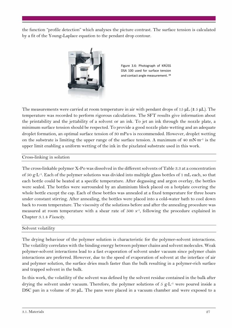
The KRÜSS DSA100, depicted in Figure 3.6, was used for surface tension (SFT) analysis of pure
solvents and inks by calculating the SFT through liquid density and two-dimensional shape analysis.
This calculation method is called the pendant drop method. The contour of the drop is extracted by
3.1. Materials 27
the function “profile detection” which analyses the picture contrast. The surface tension is calculated
by a fit of the Young-Laplace equation to the pendant drop contour.
Figure 3.6: Photograph of KRÜSS
DSA 100 used for surface tension
and contact angle measurement. 44
The measurements were carried at room temperature in air with pendant drops of 15 µL (± 5 µL). The
temperature was recorded to perform rigorous calculations. The SFT results give information about
the printability and the jettability of a solvent or an ink. To jet an ink through the nozzle plate, a
minimum surface tension should be respected. To provide a good nozzle plate wetting and an adequate
droplet formation, an optimal surface tension of 30 mPa∙s is recommended. However, droplet wetting
on the substrate is limiting the upper range of the surface tension. A maximum of 40 mN∙m-1 is the
upper limit enabling a uniform wetting of the ink in the pixelated substrate used in this work.
Cross-linking in solution
The cross-linkable polymer X-Po was dissolved in the different solvents of Table 3.3 at a concentration
of 50 g∙L-1. Each of the polymer solutions was divided into multiple glass bottles of 1 mL each, so that
each bottle could be heated at a specific temperature. After degassing and argon overlay, the bottles
were sealed. The bottles were surrounded by an aluminium block placed on a hotplate covering the
whole bottle except the cap. Each of these bottles was annealed at a fixed temperature for three hours
under constant stirring. After annealing, the bottles were placed into a cold-water bath to cool down
back to room temperature. The viscosity of the solutions before and after the annealing procedure was
measured at room temperature with a shear rate of 500 s-1, following the procedure explained in
Chapter 3.1.4 Viscocity.
Solvent volatility
The drying behaviour of the polymer solution is characteristic for the polymer-solvent interactions.
The volatility correlates with the binding energy between polymer chains and solvent molecules. Weak
polymer-solvent interactions lead to a fast evaporation of solvent under vacuum since polymer chain
interactions are preferred. However, due to the speed of evaporation of solvent at the interface of air
and polymer solution, the surface dries much faster than the bulk resulting in a polymer-rich surface
and trapped solvent in the bulk.
In this work, the volatility of the solvent was defined by the solvent residue contained in the bulk after
drying the solvent under vacuum. Therefore, the polymer solutions of 5 g∙L-1 were poured inside a
DSC pan in a volume of 30 µL. The pans were placed in a vacuum chamber and were exposed to a
28 3.Investigated System and Methods
pressure of 10-4 mbar for two hours. The volatility of a solvent from the polymer solution was
calculated as:
𝑟𝑠 =𝑚𝑠
𝑚𝑓· 100 (3.2)
𝑚𝑠 = 𝑚𝑓 − (𝑐 ·𝑚𝑖
𝑑𝑠) (3.3)
where 𝑟𝑠 is the solvent residue in weight percent, 𝑚𝑠 is the mass of solvent residual in bulk, 𝑚𝑓is the
total mass after drying of material and solvent residue, 𝑐 is the polymer solution concentration, 𝑚𝑖 is
the mass of the wet film and 𝑑𝑠 is the solvent density.
3.2. Processing of an inkjet printed layer
As introduced in Chapter 2.1.1, solution processing is offering a high material utilisation and is
therefore the most cost-effective deposition technique for OLED devices. Due to the high precision at
which the material is deposited onto a substrate, inkjet printing is a promising technology for high
resolution display applications.
3.2.1. Inkjet printer
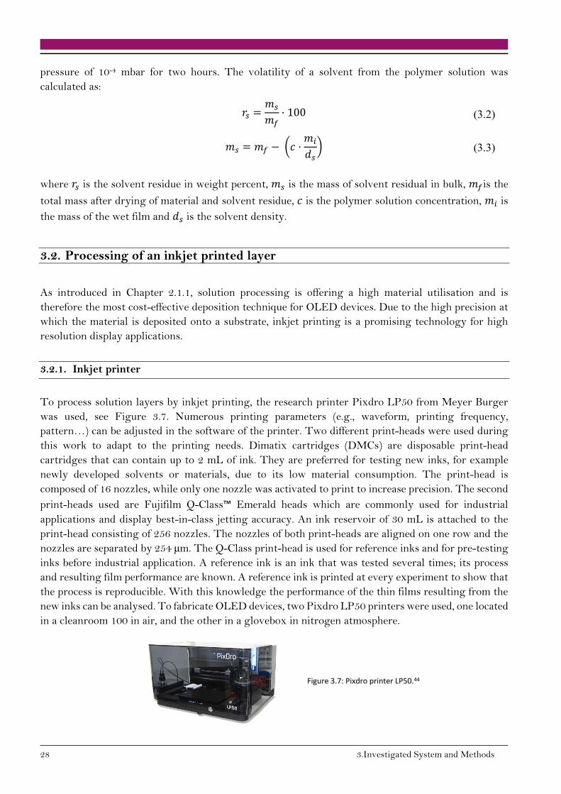
To process solution layers by inkjet printing, the research printer Pixdro LP50 from Meyer Burger
was used, see Figure 3.7. Numerous printing parameters (e.g., waveform, printing frequency,
pattern…) can be adjusted in the software of the printer. Two different print-heads were used during
this work to adapt to the printing needs. Dimatix cartridges (DMCs) are disposable print-head
cartridges that can contain up to 2 mL of ink. They are preferred for testing new inks, for example
newly developed solvents or materials, due to its low material consumption. The print-head is
composed of 16 nozzles, while only one nozzle was activated to print to increase precision. The second
print-heads used are Fujifilm Q-Class™ Emerald heads which are commonly used for industrial
applications and display best-in-class jetting accuracy. An ink reservoir of 30 mL is attached to the
print-head consisting of 256 nozzles. The nozzles of both print-heads are aligned on one row and the
nozzles are separated by 254 µm. The Q-Class print-head is used for reference inks and for pre-testing
inks before industrial application. A reference ink is an ink that was tested several times; its process
and resulting film performance are known. A reference ink is printed at every experiment to show that
the process is reproducible. With this knowledge the performance of the thin films resulting from the
new inks can be analysed. To fabricate OLED devices, two Pixdro LP50 printers were used, one located
in a cleanroom 100 in air, and the other in a glovebox in nitrogen atmosphere.
Figure 3.7: Pixdro printer LP50.44
3.2. Processing of an inkjet printed layer 29
3.2.2. Printing substrates
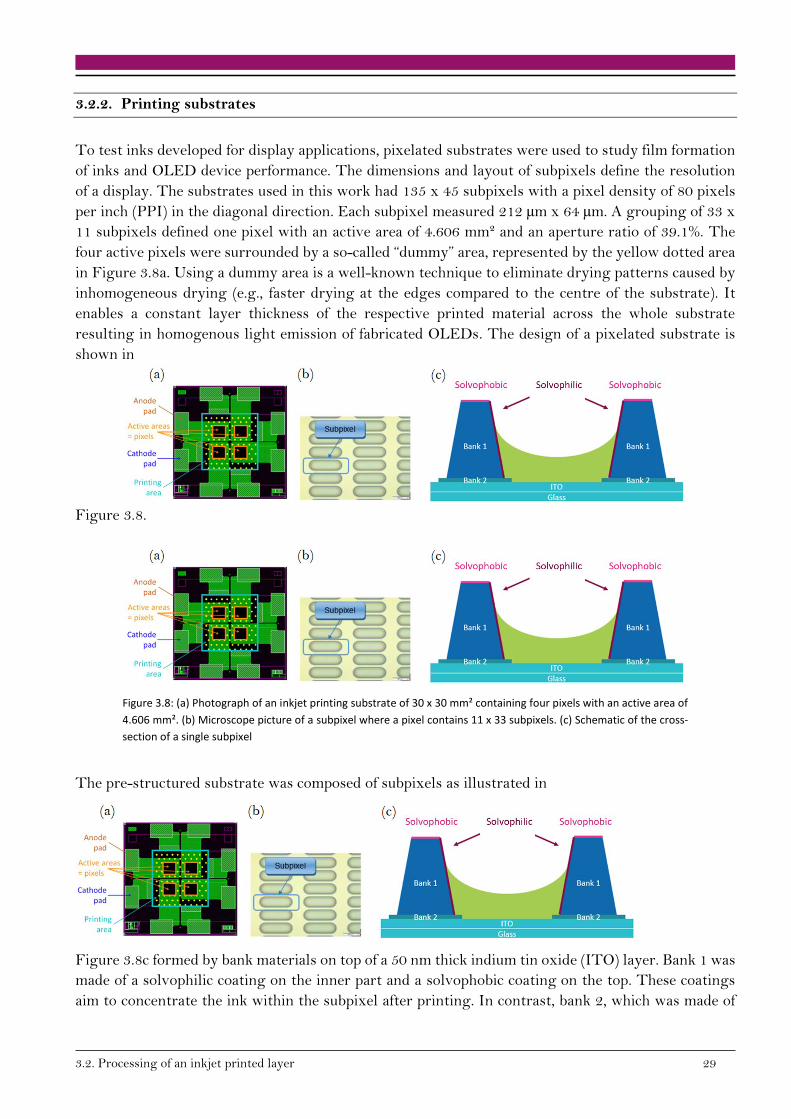
To test inks developed for display applications, pixelated substrates were used to study film formation
of inks and OLED device performance. The dimensions and layout of subpixels define the resolution
of a display. The substrates used in this work had 135 x 45 subpixels with a pixel density of 80 pixels
per inch (PPI) in the diagonal direction. Each subpixel measured 212 µm x 64 µm. A grouping of 33 x
11 subpixels defined one pixel with an active area of 4.606 mm² and an aperture ratio of 39.1%. The
four active pixels were surrounded by a so-called “dummy” area, represented by the yellow dotted area
in Figure 3.8a. Using a dummy area is a well-known technique to eliminate drying patterns caused by
inhomogeneous drying (e.g., faster drying at the edges compared to the centre of the substrate). It
enables a constant layer thickness of the respective printed material across the whole substrate
resulting in homogenous light emission of fabricated OLEDs. The design of a pixelated substrate is
shown in
Figure 3.8.
Figure 3.8: (a) Photograph of an inkjet printing substrate of 30 x 30 mm² containing four pixels with an active area of
4.606 mm². (b) Microscope picture of a subpixel where a pixel contains 11 x 33 subpixels. (c) Schematic of the cross-
section of a single subpixel
The pre-structured substrate was composed of subpixels as illustrated in
Figure 3.8c formed by bank materials on top of a 50 nm thick indium tin oxide (ITO) layer. Bank 1 was
made of a solvophilic coating on the inner part and a solvophobic coating on the top. These coatings
aim to concentrate the ink within the subpixel after printing. In contrast, bank 2, which was made of

30 3.Investigated System and Methods
insulating silicon dioxide, was used to increase the homogeneity of the layer thickness of printed
OLEDs as will be explained in the next section.
Figure 3.9: (a) Microscope picture of one subpixel. (b) SEM picture of bank 1 and bank 2 with one
organic layer printed in subpixel. Picture taken from the side. (c) Film profile in subpixel measured
by profilometer. The outer region of the subpixel is depicted by a red dashed box.
In the outer region of a subpixel emphasised by a red dashed box in Figure 3.9, it is often seen that the
layer is not uniform due to adhesion on the bank material. Because of the insulating bank 2, no electrical
current can be injected into the organic layers in the outer regions of the subpixel and thus only the
flat and uniform layer in the centre of the subpixel contributes to light emission of the OLED device.
The film formation inside a subpixel is presented in Chapter 6.1.2.
In addition to the pre-patterned substrates presented above, bare glass substrates of 30 mm x 30 mm
were used for film stability tests against solvent exposure and for optical measurements of printed
films, which were carried out on large area films.
3.2.3. Film formation process
Printing
The printing speed has a direct impact on the printing quality, i.e., the film homogeneity and the
droplet landing precision. An increase in printing speed can lead to higher film homogeneity since the
drying start with a shorter delay between the first and last printed droplet.76 However, a maximum
printing speed should not be exceeded; otherwise it could also result in a heterogeneous droplet
spacing, thus a discontinuous printing resolution. With the Pixdro LP50 printer, a maximum of 250
m∙s-1 printing speed is possible. Only one nozzle was used to jet the ink droplet and the printing was
bi-directional. The printing speed was then adjusted to reach an intended droplet spacing according to
Eq. 3.4.
𝑣𝑝𝑟𝑖𝑛𝑡 = 𝐷𝑆 · 𝑓 (3.4)
where 𝑣𝑝𝑟𝑖𝑛𝑡 is the printing speed in m∙s-1, 𝐷𝑆 is the droplet spacing in metre and 𝑓 is the printing
frequency in s-1. The droplet spacing was utilised to vary and tune the layer thickness. The printing
time varied between 20 seconds to 100 seconds.

3.2. Processing of an inkjet printed layer 31
Drying
Figure 3.10: Pressure profiles
with time in the vacuum chamber
in dependence on the selected
drying speed.
After printing the ink into the subpixels, the high boiling point solvent had to be removed prior to the
thermal annealing step. The vacuum dryer was equipped with two different pumps in order to achieve
a high vacuum of 10-5-10-6 mbar at various speeds. The pressure profile in the chamber during the
vacuum drying process was tuned by pump-down programs, as depicted in Figure 3.10. The drying
conditions were adapted to the respective ink, since material-solvent mixtures behaved differently
depending on their viscosity, vapour pressure, material-solvent interaction and affinity to the bank
materials. The time to place the printing film under vacuum varied due to manual handling and it
fluctuated between 15 seconds up to 5 minutes. This duration was not identified as having an influence
on the film formation due to a fast ink levelling on the substrate.
Drying: Drying of large area films
In the beginning of the drying process, the evaporation rate of the solvent was the highest at the
substrate edges and weaker in the centre. In Figure 3.11, the drying evolution of a large area printed
film on a glass substrate can be seen. The drying does not start homogeneously over the layer due to
disparate vapour pressure at the layer edges compared to the centre of the layer.

32 3.Investigated System and Methods
Figure 3.11: Photographs of a large area film during the drying process in the vacuum chamber taken by camera under UV
illumination. An emissive material mixture was printed from menthyl isovalerate on glass substrate and dried with the slow drying
speed program. For an easier identification at t = 0 s and t = 127 s, the substrate has been marked in grey, the wet film in white
and the dry film in orange.
Drying: Drying in a patterned substrate with banks
In a patterned substrate, the solvent evaporation was more complex than for the large area films. After
the ink level has dropped below the bank height, a capillary suction from the bank walls occurred due
to the negative curvature of the drop. This negative curvature was caused by the droplet pinning at
the top of the bank wall.97 The dried film pinned on bank 1 and bank 2 as can be seen in Figure 3.9b.
Due to the insulating material composing the banks, the part of the printed film pinned on the banks
did not conduct charge carriers.
Annealing
After drying, the substrate was transferred to a N2-filled glovebox where thermal annealing was
performed on a hotplate. This thermal treatment was necessary to trigger the cross-linking reaction
of the HIL and the HTL. For the EML, thermal treatment was also utilised to remove solvent residue
from the layer. The substrate was placed on a hotplate, printing side up, at a fixed and stable
temperature for various times depending on the layer. The HIL and HTL were annealed for 30 minutes
at 225°C (the HTL annealing temperature was varied in the study) and the EML was treated for 10
minutes at 150°C.
3.2.4. Film thickness measurement
Film thickness determination was carried out on thin films after being inkjet printed, vacuum dried
and annealed. The layer profile was measured by the profilometer Dektak 150 from Veeco Instruments
Inc. utilising a diamond needle.
Large area films
To determine the thickness of large area printed films, the printed layer was scratched with a scalpel
so that the cross-section was accessible to the measurement. Subsequently, the needle of the
profilometer was moved perpendicular to this scratch and the deflection of the needle was recorded.
The needle scanned a defined length and recorded points every 100 nm with a contact force of 5 mN.
The precision of the thickness measurement was ±2 nm.
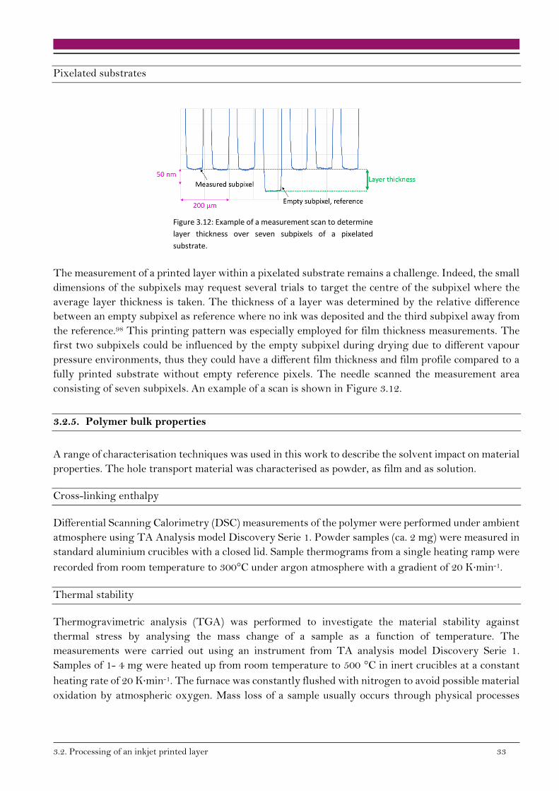
3.2. Processing of an inkjet printed layer 33
Pixelated substrates
Figure 3.12: Example of a measurement scan to determine
layer thickness over seven subpixels of a pixelated
substrate.
The measurement of a printed layer within a pixelated substrate remains a challenge. Indeed, the small
dimensions of the subpixels may request several trials to target the centre of the subpixel where the
average layer thickness is taken. The thickness of a layer was determined by the relative difference
between an empty subpixel as reference where no ink was deposited and the third subpixel away from
the reference.98 This printing pattern was especially employed for film thickness measurements. The
first two subpixels could be influenced by the empty subpixel during drying due to different vapour
pressure environments, thus they could have a different film thickness and film profile compared to a
fully printed substrate without empty reference pixels. The needle scanned the measurement area
consisting of seven subpixels. An example of a scan is shown in Figure 3.12.
3.2.5. Polymer bulk properties
A range of characterisation techniques was used in this work to describe the solvent impact on material
properties. The hole transport material was characterised as powder, as film and as solution.
Cross-linking enthalpy
Differential Scanning Calorimetry (DSC) measurements of the polymer were performed under ambient
atmosphere using TA Analysis model Discovery Serie 1. Powder samples (ca. 2 mg) were measured in
standard aluminium crucibles with a closed lid. Sample thermograms from a single heating ramp were
recorded from room temperature to 300°C under argon atmosphere with a gradient of 20 K∙min-1.
Thermal stability
Thermogravimetric analysis (TGA) was performed to investigate the material stability against
thermal stress by analysing the mass change of a sample as a function of temperature. The
measurements were carried out using an instrument from TA analysis model Discovery Serie 1.
Samples of 1- 4 mg were heated up from room temperature to 500 °C in inert crucibles at a constant
heating rate of 20 K∙min-1. The furnace was constantly flushed with nitrogen to avoid possible material
oxidation by atmospheric oxygen. Mass loss of a sample usually occurs through physical processes
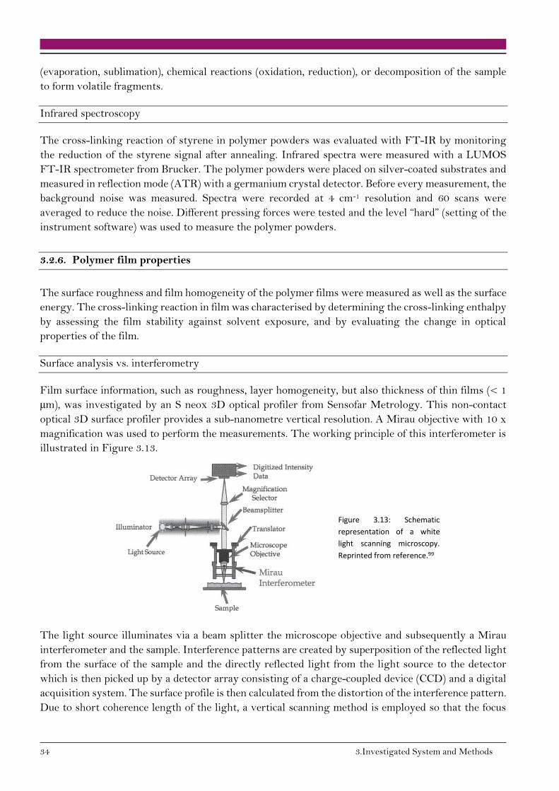
34 3.Investigated System and Methods
(evaporation, sublimation), chemical reactions (oxidation, reduction), or decomposition of the sample
to form volatile fragments.
Infrared spectroscopy
The cross-linking reaction of styrene in polymer powders was evaluated with FT-IR by monitoring
the reduction of the styrene signal after annealing. Infrared spectra were measured with a LUMOS
FT-IR spectrometer from Brucker. The polymer powders were placed on silver-coated substrates and
measured in reflection mode (ATR) with a germanium crystal detector. Before every measurement, the
background noise was measured. Spectra were recorded at 4 cm-1 resolution and 60 scans were
averaged to reduce the noise. Different pressing forces were tested and the level “hard” (setting of the
instrument software) was used to measure the polymer powders.
3.2.6. Polymer film properties
The surface roughness and film homogeneity of the polymer films were measured as well as the surface
energy. The cross-linking reaction in film was characterised by determining the cross-linking enthalpy
by assessing the film stability against solvent exposure, and by evaluating the change in optical
properties of the film.
Surface analysis vs. interferometry
Film surface information, such as roughness, layer homogeneity, but also thickness of thin films (< 1
µm), was investigated by an S neox 3D optical profiler from Sensofar Metrology. This non-contact
optical 3D surface profiler provides a sub-nanometre vertical resolution. A Mirau objective with 10 x
magnification was used to perform the measurements. The working principle of this interferometer is
illustrated in Figure 3.13.
Figure 3.13: Schematic
representation of a white
light scanning microscopy.
Reprinted from reference.99
The light source illuminates via a beam splitter the microscope objective and subsequently a Mirau
interferometer and the sample. Interference patterns are created by superposition of the reflected light
from the surface of the sample and the directly reflected light from the light source to the detector
which is then picked up by a detector array consisting of a charge-coupled device (CCD) and a digital
acquisition system. The surface profile is then calculated from the distortion of the interference pattern.
Due to short coherence length of the light, a vertical scanning method is employed so that the focus
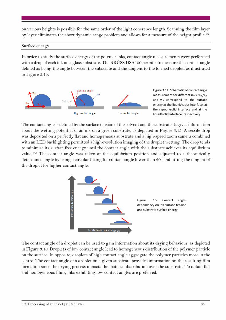
3.2. Processing of an inkjet printed layer 35
on various heights is possible for the same order of the light coherence length. Scanning the film layer
by layer eliminates the short dynamic range problem and allows for a measure of the height profile.99
Surface energy
In order to study the surface energy of the polymer inks, contact angle measurements were performed
with a drop of each ink on a glass substrate. The KRÜSS DSA100 permits to measure the contact angle
defined as being the angle between the substrate and the tangent to the formed droplet, as illustrated
in Figure 3.14.
Figure 3.14: Schematic of contact angle
measurement for different inks. γVL, γVS
and γLS correspond to the surface
energy at the liquid/vapor interface, at
the vapour/solid interface and at the
liquid/solid interface, respectively.
The contact angle is defined by the surface tension of the solvent and the substrate. It gives information
about the wetting potential of an ink on a given substrate, as depicted in Figure 3.15. A sessile drop
was deposited on a perfectly flat and homogeneous substrate and a high-speed zoom camera combined
with an LED backlighting permitted a high-resolution imaging of the droplet wetting. The drop tends
to minimise its surface free energy until the contact angle with the substrate achieves its equilibrium
value.100 The contact angle was taken at the equilibrium position and adjusted to a theoretically
determined angle by using a circular fitting for contact angle lower than 20° and fitting the tangent of
the droplet for higher contact angle.
Figure 3.15: Contact angle-
dependency on ink surface tension
and substrate surface energy.
The contact angle of a droplet can be used to gain information about its drying behaviour, as depicted
in Figure 3.16. Droplets of low contact angle lead to homogeneous distribution of the polymer particle
on the surface. In opposite, droplets of high contact angle aggregate the polymer particles more in the
centre. The contact angle of a droplet on a given substrate provides information on the resulting film
formation since the drying process impacts the material distribution over the substrate. To obtain flat
and homogeneous films, inks exhibiting low contact angles are preferred.
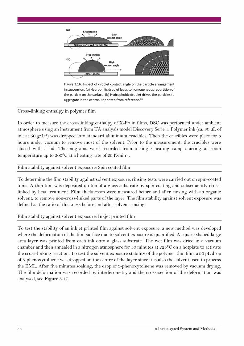
36 3.Investigated System and Methods
Figure 3.16: Impact of droplet contact angle on the particle arrangement
in suspension. (a) Hydrophilic droplet leads to homogeneous repartition of
the particle on the surface. (b) Hydrophobic droplet drives the particles to
aggregate in the centre. Reprinted from reference.66
Cross-linking enthalpy in polymer film
In order to measure the cross-linking enthalpy of X-Po in films, DSC was performed under ambient
atmosphere using an instrument from TA analysis model Discovery Serie 1. Polymer ink (ca. 30 µL of
ink at 50 g·L-1) was dropped into standard aluminium crucibles. Then the crucibles were place for 3
hours under vacuum to remove most of the solvent. Prior to the measurement, the crucibles were
closed with a lid. Thermograms were recorded from a single heating ramp starting at room
temperature up to 300°C at a heating rate of 20 K∙min-1.
Film stability against solvent exposure: Spin coated film
To determine the film stability against solvent exposure, rinsing tests were carried out on spin-coated
films. A thin film was deposited on top of a glass substrate by spin-coating and subsequently cross-
linked by heat treatment. Film thicknesses were measured before and after rinsing with an organic
solvent, to remove non-cross-linked parts of the layer. The film stability against solvent exposure was
defined as the ratio of thickness before and after solvent rinsing.
Film stability against solvent exposure: Inkjet printed film
To test the stability of an inkjet printed film against solvent exposure, a new method was developed
where the deformation of the film surface due to solvent exposure is quantified. A square shaped large
area layer was printed from each ink onto a glass substrate. The wet film was dried in a vacuum
chamber and then annealed in a nitrogen atmosphere for 30 minutes at 225°C on a hotplate to activate
the cross-linking reaction. To test the solvent exposure stability of the polymer thin film, a 90 pL drop
of 3-phenoxytoluene was dropped on the centre of the layer since it is also the solvent used to process
the EML. After five minutes soaking, the drop of 3-phenoxytoluene was removed by vacuum drying.
The film deformation was recorded by interferometry and the cross-section of the deformation was
analysed, see Figure 3.17.
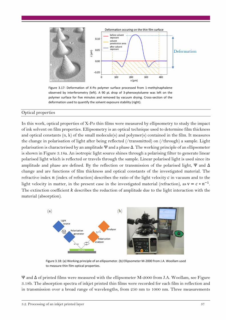
3.2. Processing of an inkjet printed layer 37
Figure 3.17: Deformation of X-Po polymer surface processed from 1-methylnaphalene
observed by interferometry (left). A 90 pL drop of 3-phenoxytoluene was left on the
polymer surface for five minutes and removed by vacuum drying. Cross-section of the
deformation used to quantify the solvent exposure stability (right).
Optical properties
In this work, optical properties of X-Po thin films were measured by ellipsometry to study the impact
of ink solvent on film properties. Ellipsometry is an optical technique used to determine film thickness
and optical constants (n, k) of the small molecule(s) and polymer(s) contained in the film. It measures
the change in polarisation of light after being reflected (/transmitted) on (/through) a sample. Light
polarisation is characterised by an amplitude Ψ and a phase Δ. The working principle of an ellipsometer
is shown in Figure 3.18a. An isotropic light source shines through a polarising filter to generate linear
polarised light which is reflected or travels through the sample. Linear polarised light is used since its
amplitude and phase are defined. By the reflection or transmission of the polarised light, Ψ and Δ
change and are functions of film thickness and optical constants of the investigated material. The
refractive index 𝑛 (index of refraction) describes the ratio of the light velocity 𝑐 in vacuum and to the
light velocity in matter, in the present case in the investigated material (refraction), as v = 𝑐 ∗ 𝑛−1.
The extinction coefficient 𝑘 describes the reduction of amplitude due to the light interaction with the
material (absorption).
Figure 3.18: (a) Working principle of an ellipsometer. (b) Ellipsometer M-2000 from J.A. Woollam used
to measure thin film optical properties.
Ψ and Δ of printed films were measured with the ellipsometer M-2000 from J.A. Woollam, see Figure
3.18b. The absorption spectra of inkjet printed thin films were recorded for each film in reflection and
in transmission over a broad range of wavelengths, from 250 nm to 1000 nm. Three measurements
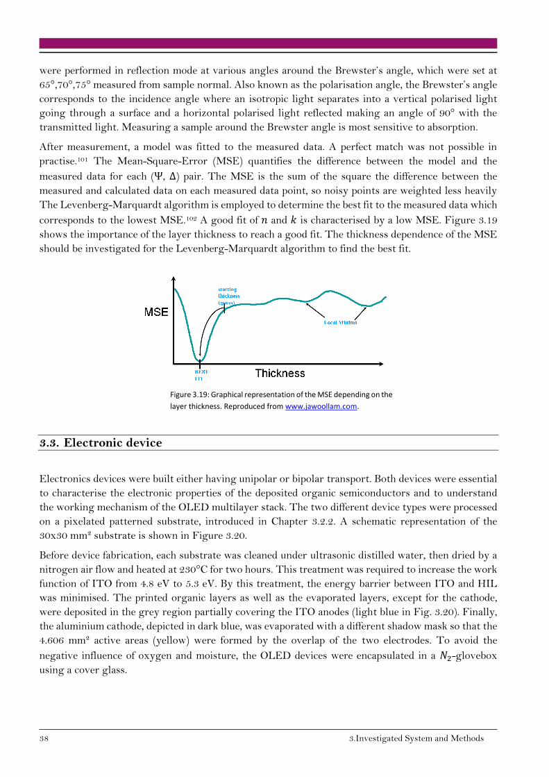
38 3.Investigated System and Methods
were performed in reflection mode at various angles around the Brewster’s angle, which were set at
65°,70°,75° measured from sample normal. Also known as the polarisation angle, the Brewster’s angle
corresponds to the incidence angle where an isotropic light separates into a vertical polarised light
going through a surface and a horizontal polarised light reflected making an angle of 90° with the
transmitted light. Measuring a sample around the Brewster angle is most sensitive to absorption.
After measurement, a model was fitted to the measured data. A perfect match was not possible in
practise.101 The Mean-Square-Error (MSE) quantifies the difference between the model and the
measured data for each (Ψ, Δ) pair. The MSE is the sum of the square the difference between the
measured and calculated data on each measured data point, so noisy points are weighted less heavily
The Levenberg-Marquardt algorithm is employed to determine the best fit to the measured data which
corresponds to the lowest MSE.102 A good fit of 𝑛 and 𝑘 is characterised by a low MSE. Figure 3.19
shows the importance of the layer thickness to reach a good fit. The thickness dependence of the MSE
should be investigated for the Levenberg-Marquardt algorithm to find the best fit.
Figure 3.19: Graphical representation of the MSE depending on the
layer thickness. Reproduced from www.jawoollam.com.
3.3. Electronic device
Electronics devices were built either having unipolar or bipolar transport. Both devices were essential
to characterise the electronic properties of the deposited organic semiconductors and to understand
the working mechanism of the OLED multilayer stack. The two different device types were processed
on a pixelated patterned substrate, introduced in Chapter 3.2.2. A schematic representation of the
30x30 mm² substrate is shown in Figure 3.20.
Before device fabrication, each substrate was cleaned under ultrasonic distilled water, then dried by a
nitrogen air flow and heated at 230°C for two hours. This treatment was required to increase the work
function of ITO from 4.8 eV to 5.3 eV. By this treatment, the energy barrier between ITO and HIL
was minimised. The printed organic layers as well as the evaporated layers, except for the cathode,
were deposited in the grey region partially covering the ITO anodes (light blue in Fig. 3.20). Finally,
the aluminium cathode, depicted in dark blue, was evaporated with a different shadow mask so that the
4.606 mm² active areas (yellow) were formed by the overlap of the two electrodes. To avoid the
negative influence of oxygen and moisture, the OLED devices were encapsulated in a 𝑁2-glovebox
using a cover glass.

3.3. Electronic device 39
Figure 3.20: Schematic representation of a device
built for electronics characterisation. Four active
areas (yellow) are formed by the overlapping
anodes (light blue) and cathodes (dark blue). The
area in grey depicts the region where the printed as
well as evaporated layers are deposited.
3.3.1. Carrier mobility in hole transport layer
The mobility is an important parameter to characterise the transport properties of organic thin films.
The mobility can be measured by the so called Time of Flight (TOF) technique. However, this
technique requires film thickness of about 2-8 µm. Since soluble films are commonly between 10 nm
and 200 nm thick, this technique cannot be deployed. On the other hand carrier mobility can be
extracted from organic field-effect transistors (OFET) measurements. Nevertheless, the OFET
configuration determines the carrier mobility along the substrate direction. Thus this measurement
technique is meaningful only for film with anisotropic carrier mobilities.103 A third technique to
determine the mobility is the space-charge-limited current (SCLC) technique which is well established
to investigate the carrier mobility of organic thin films. The typical SCLC behaviour for polymer
semiconductors is represented in Figure 3.21. To calculate the mobility of X-Po, unipolar devices were
built insuring a good Ohmic contact between the organic layer and the injecting metal electrode.
Figure 3.21: Typical space charge–limited
current behaviour for polymer
semiconductor. Four charge‐transport
regions are visible (i) Ohmic region (J ∝ V), (ii)
trap‐SCLC region (J ∝ V1-2), (iii) TFL region (J ∝
V2-100), and (iv) SCLC region (J ∝ V2). Reprinted
from reference.104
Unipolar devices can be fabricated by inserting the organic layer under investigation between two
suited electrodes. The organic layers can be composed of a single or a mixture of material(s). Two
organic layers can also be studied if they ensure a single carrier transport. In unipolar devices,
recombination is absent, since only one carrier type is present.105 Measurement of unipolar devices
provide information on charge transport in an organic layer. It is obtained from a single steady-state
current–voltage measurement from the device. At low current density, the current is mainly carried
by thermal equilibrium charge carrier density. It is described by the Ohmic regime and a linear
dependency of the current density J with voltage V. The conductivity 𝜎 is described as:
𝜎 = 𝑒𝑛𝜇 (3.5)
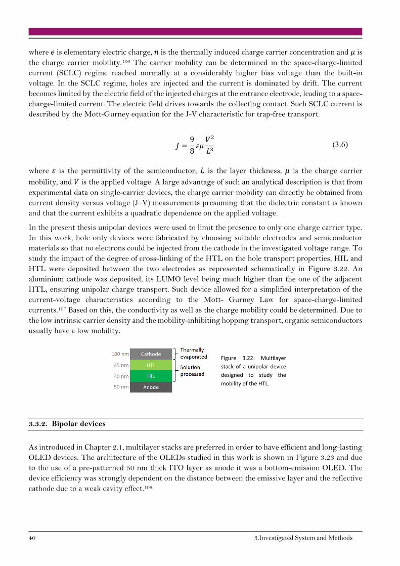
40 3.Investigated System and Methods
where 𝑒 is elementary electric charge, 𝑛 is the thermally induced charge carrier concentration and 𝜇 is
the charge carrier mobility.106 The carrier mobility can be determined in the space-charge-limited
current (SCLC) regime reached normally at a considerably higher bias voltage than the built-in
voltage. In the SCLC regime, holes are injected and the current is dominated by drift. The current
becomes limited by the electric field of the injected charges at the entrance electrode, leading to a space-
charge-limited current. The electric field drives towards the collecting contact. Such SCLC current is
described by the Mott-Gurney equation for the J-V characteristic for trap-free transport:
𝐽 =9
8𝜀𝜇
𝑉2
𝐿3 (3.6)
where 𝜀 is the permittivity of the semiconductor, 𝐿 is the layer thickness, 𝜇 is the charge carrier
mobility, and 𝑉 is the applied voltage. A large advantage of such an analytical description is that from
experimental data on single-carrier devices, the charge carrier mobility can directly be obtained from
current density versus voltage (J–V) measurements presuming that the dielectric constant is known
and that the current exhibits a quadratic dependence on the applied voltage.
In the present thesis unipolar devices were used to limit the presence to only one charge carrier type.
In this work, hole only devices were fabricated by choosing suitable electrodes and semiconductor
materials so that no electrons could be injected from the cathode in the investigated voltage range. To
study the impact of the degree of cross-linking of the HTL on the hole transport properties, HIL and
HTL were deposited between the two electrodes as represented schematically in Figure 3.22. An
aluminium cathode was deposited, its LUMO level being much higher than the one of the adjacent
HTL, ensuring unipolar charge transport. Such device allowed for a simplified interpretation of the
current-voltage characteristics according to the Mott- Gurney Law for space-charge-limited
currents.107 Based on this, the conductivity as well as the charge mobility could be determined. Due to
the low intrinsic carrier density and the mobility-inhibiting hopping transport, organic semiconductors
usually have a low mobility.
Figure 3.22: Multilayer
stack of a unipolar device
designed to study the
mobility of the HTL.
3.3.2. Bipolar devices
As introduced in Chapter 2.1, multilayer stacks are preferred in order to have efficient and long-lasting
OLED devices. The architecture of the OLEDs studied in this work is shown in Figure 3.23 and due
to the use of a pre-patterned 50 nm thick ITO layer as anode it was a bottom-emission OLED. The
device efficiency was strongly dependent on the distance between the emissive layer and the reflective
cathode due to a weak cavity effect.108
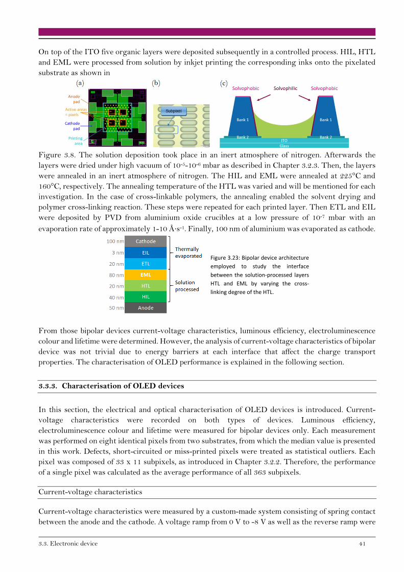
3.3. Electronic device 41
On top of the ITO five organic layers were deposited subsequently in a controlled process. HIL, HTL
and EML were processed from solution by inkjet printing the corresponding inks onto the pixelated
substrate as shown in
Figure 3.8. The solution deposition took place in an inert atmosphere of nitrogen. Afterwards the
layers were dried under high vacuum of 10-5-10-6 mbar as described in Chapter 3.2.3. Then, the layers
were annealed in an inert atmosphere of nitrogen. The HIL and EML were annealed at 225°C and
160°C, respectively. The annealing temperature of the HTL was varied and will be mentioned for each
investigation. In the case of cross-linkable polymers, the annealing enabled the solvent drying and
polymer cross-linking reaction. These steps were repeated for each printed layer. Then ETL and EIL
were deposited by PVD from aluminium oxide crucibles at a low pressure of 10-7 mbar with an
evaporation rate of approximately 1-10 Å∙s-1. Finally, 100 nm of aluminium was evaporated as cathode.
Figure 3.23: Bipolar device architecture
employed to study the interface
between the solution-processed layers
HTL and EML by varying the cross-
linking degree of the HTL.
From those bipolar devices current-voltage characteristics, luminous efficiency, electroluminescence
colour and lifetime were determined. However, the analysis of current-voltage characteristics of bipolar
device was not trivial due to energy barriers at each interface that affect the charge transport
properties. The characterisation of OLED performance is explained in the following section.
3.3.3. Characterisation of OLED devices
In this section, the electrical and optical characterisation of OLED devices is introduced. Current-
voltage characteristics were recorded on both types of devices. Luminous efficiency,
electroluminescence colour and lifetime were measured for bipolar devices only. Each measurement
was performed on eight identical pixels from two substrates, from which the median value is presented
in this work. Defects, short-circuited or miss-printed pixels were treated as statistical outliers. Each
pixel was composed of 33 x 11 subpixels, as introduced in Chapter 3.2.2. Therefore, the performance
of a single pixel was calculated as the average performance of all 363 subpixels.
Current-voltage characteristics
Current-voltage characteristics were measured by a custom-made system consisting of spring contact
between the anode and the cathode. A voltage ramp from 0 V to -8 V as well as the reverse ramp were
42 3.Investigated System and Methods
applied by a Keithley 2400 SourceMeter. Simultaneously, the current of each pixel was measured by a
Keithley 2700 MultiMeter in the dark. The maximum voltage was chosen such that the maximum
current density did not exceed 100 mA∙cm-². In the case of hole-only devices, the measurements were
recorded for voltages from 0 to 2 V in steps of 20 mV, afterwards steps of 0.2 V were applied until a
current density of 100 mA∙cm-² was reached. In the low current density range, each measurement point
was averaged over a period of 200 milliseconds to ensure that the current measurements were able to
reach a steady-state. The current 𝐼 through the device was measured and the current density 𝑗 was
calculated by the relationship:
𝑗 =𝐼
𝐴 (3.7)
where 𝑗 is recorded in mA∙cm-², 𝐼 is the current in mA and 𝐴 is the active luminous area with 𝐴 = 4.606
mm².
Luminous efficiency
Simultaneously to the I-V characteristic, the incident photon flux was measured by a calibrated
photodiode connected to a Keithley 6485 Picoamperemeter. In order to convert the measured photon
flux into luminance in cd∙m-², the photodiode was calibrated by the photometer LMT L1009 of
LichtMessTechnik GmbH in combination with a V(λ) filter. The photopic luminous function V(λ)
represents the light sensitivity curve of the human eye within the photopic wavelength range. The
luminous efficiency 𝜂𝐿 of OLED devices (units cd∙A-1) is determined as the ratio of the luminance 𝐿
(units cd∙m-2) and the current density 𝑗 (units mA∙cm-2), as followed:
𝜂𝐿 =𝐿
𝑗 (3.8)
Another method to quantify the efficiency of OLEDs is the external quantum efficiency (EQE, 𝜂𝑒𝑥𝑡).
The EQE is defined as the ratio of the extracted photons to the number of majority charge carriers
injected, as described by:
𝜂𝑒𝑥𝑡 = 𝜂𝑓 · 𝛾𝑒−ℎ · 𝜒𝑠/𝑡 · 𝜑𝑜𝑝𝑡. (3.9)
Here, 𝜂𝑓 is the yield of radiative decay from singlet excitons, 𝛾𝑒−ℎ is the charge carrier balance between
injected holes and electrons in the EML (should be ideally 1), 𝜒𝑠/𝑡 is the fraction of generated excitons
which can decay radiatively (0.25 in fluorescence, 1 in phosphorescence) and 𝜑𝑜𝑝𝑡 is the outcoupling
efficiency defined by the ratio of light emitted at the surface to the light produced in the bulk of the
device (estimated to 20%). However, directly measuring the number of photons emitted from a device
is challenging. Therefore, commonly the EQE is determined from the I-V-L characteristics and the
electroluminescence spectrum.
Electroluminescence
The colour of the emitted light from the OLED pixels was characterised using an Ocean Optic
USB4000 fibre optic spectrometer. The emission spectra were recorded at a luminance of 1000 cd∙m-2
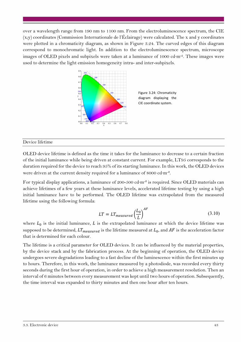
3.3. Electronic device 43
over a wavelength range from 190 nm to 1100 nm. From the electroluminescence spectrum, the CIE
(x;y) coordinates (Commission Internationale de l’Éclairage) were calculated. The x and y coordinates
were plotted in a chromaticity diagram, as shown in Figure 3.24. The curved edges of this diagram
correspond to monochromatic light. In addition to the electroluminescence spectrum, microscope
images of OLED pixels and subpixels were taken at a luminance of 1000 cd∙m-2. These images were
used to determine the light emission homogeneity intra- and inter-subpixels.
Figure 3.24: Chromaticity
diagram displaying the
CIE coordinate system.
Device lifetime
OLED device lifetime is defined as the time it takes for the luminance to decrease to a certain fraction
of the initial luminance while being driven at constant current. For example, LT95 corresponds to the
duration required for the device to reach 95% of its starting luminance. In this work, the OLED devices
were driven at the current density required for a luminance of 8000 cd∙m-².
For typical display applications, a luminance of 200-500 cd∙m-² is required. Since OLED materials can
achieve lifetimes of a few years at these luminance levels, accelerated lifetime testing by using a high
initial luminance have to be performed. The OLED lifetime was extrapolated from the measured
lifetime using the following formula:
𝐿𝑇 = 𝐿𝑇𝑚𝑒𝑎𝑠𝑢𝑟𝑒𝑑 (𝐿0
𝐿)
𝐴𝐹
(3.10)
where 𝐿0 is the initial luminance, 𝐿 is the extrapolated luminance at which the device lifetime was
supposed to be determined, 𝐿𝑇𝑚𝑒𝑎𝑠𝑢𝑟𝑒𝑑 is the lifetime measured at 𝐿0, and 𝐴𝐹 is the acceleration factor
that is determined for each colour.
The lifetime is a critical parameter for OLED devices. It can be influenced by the material properties,
by the device stack and by the fabrication process. At the beginning of operation, the OLED device
undergoes severe degradations leading to a fast decline of the luminescence within the first minutes up
to hours. Therefore, in this work, the luminance measured by a photodiode, was recorded every thirty
seconds during the first hour of operation, in order to achieve a high measurement resolution. Then an
interval of 6 minutes between every measurement was kept until two hours of operation. Subsequently,
the time interval was expanded to thirty minutes and then one hour after ten hours.

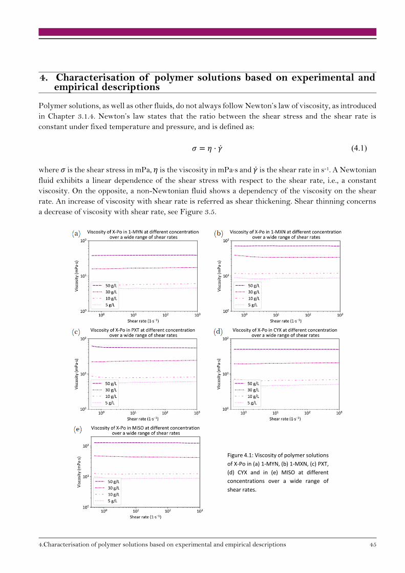
4.Characterisation of polymer solutions based on experimental and empirical descriptions 45
4. Characterisation of polymer solutions based on experimental and empirical descriptions
Polymer solutions, as well as other fluids, do not always follow Newton’s law of viscosity, as introduced
in Chapter 3.1.4. Newton’s law states that the ratio between the shear stress and the shear rate is
constant under fixed temperature and pressure, and is defined as:
𝜎 = 𝜂 · �̇� (4.1)
where 𝜎 is the shear stress in mPa, 𝜂 is the viscosity in mPa∙s and �̇� is the shear rate in s-1. A Newtonian
fluid exhibits a linear dependence of the shear stress with respect to the shear rate, i.e., a constant
viscosity. On the opposite, a non-Newtonian fluid shows a dependency of the viscosity on the shear
rate. An increase of viscosity with shear rate is referred as shear thickening. Shear thinning concerns
a decrease of viscosity with shear rate, see Figure 3.5.
Figure 4.1: Viscosity of polymer solutions
of X-Po in (a) 1-MYN, (b) 1-MXN, (c) PXT,
(d) CYX and in (e) MISO at different
concentrations over a wide range of
shear rates.
46 4.Characterisation of polymer solutions based on experimental and empirical descriptions
Newtonian and non-Newtonian fluids respond to different laws and cannot be characterised by the
same models. In order to identify the properties of polymer X-Po solutions, numerous viscosity
measurements have been carried out. Polymer X-Po was dissolved in 1-methylnaphthalene, 1-
methoxynaphthalene, 3-phenoxytoluene, cyclohexyl hexanoate and in menthyl isovalerate at the
concentrations of 5 g∙L-1, 10 g∙L-1, 30 g∙L-1 and 50 g∙L-1. The viscosity dependency on the shear rate is
plotted to identify whether the solutions follow the Newton’s viscosity law, and if not, from which
concentration the behaviour deviates from the Newtonian viscosity, see Figure 4.1.
For all polymer solutions at all tested concentrations, the viscosities are constant over a wide range of
shear rates from 0.5 s-1 to 1000 s-1. It is concluded that the polymer solutions of X-Po in 1-
methylnaphthalene, 1-methoxynaphthalene, 3-phenoxytoluene, cyclohexyl hexanoate and in menthyl
isovalerate at the concentration of 5 g∙L-1, 10 g∙L-1, 30 g∙L-1 and 50 g∙L-1 are all following Newton’s
law of viscosity.
In this chapter, the affinity of X-Po polymer with the processing solvent is characterised by
experimental measurements as well as empirical descriptions such as the Mark-Houwink parameters,
the Huggins and Kramer constants, and the Solomon Ciuta equation.
4.1. Polymer-solvent affinity
The affinity between a polymer and a solvent characterises the interaction occurring between the
polymer chains and the solvent molecules. The polymer-solvent interaction directly impacts the size
and conformation of a polymer chain in solution, defined by its hydrodynamic volume. A solvent
exhibiting a low interaction with a polymer leads to enhanced intramolecular interactions resulting in
a decrease of the hydrodynamic volume, i.e., a smaller radius of gyration Rg.109 This solvent is called a
bad or poor solvent for the given polymer: the polymer chains tend to minimise their interaction with
the solvent molecules. A “theta” solvent corresponds to an intermediate state where the polymer acts
like ideal chains, presuming a random coil conformation. When polymer chains expand and tend to
maximise their contact with the solvent molecules, the solvent is called good.
4.1.1. Experimental determination of polymer-solvent affinity
Solubility of a polymer in a solvent describes the ability of the solute to favourably interact with the
solvent. It depends on the polymer and solvent properties, as well as environmental factors like
temperature and pressure. The Hildebrand-Scott equation presents the relationship between the
polymer solubility and the polymer-solvent interaction.110 The Hildebrand-Scott equation will not be
discussed in details in this work. It simply states that the polymer-solvent interaction is directly
proportional to the Hildebrand solubility parameters of the polymer and the solvent. So, solubility of
a polymer in a solvent is a parameter that can be used to investigate the interaction between polymer
and solvent.111
Practically, the maximum solubility is described by the saturation concentration of a material in a
solvent. Starting from saturation concentration and adding more material triggers precipitation of the
excess of material. The solubility of X-Po was measured in 1-methylnaphthalene, 1-
methoxynaphthalene, 3-phenoxytoluene, cyclohexyl hexanoate and in menthyl isovalerate. However,
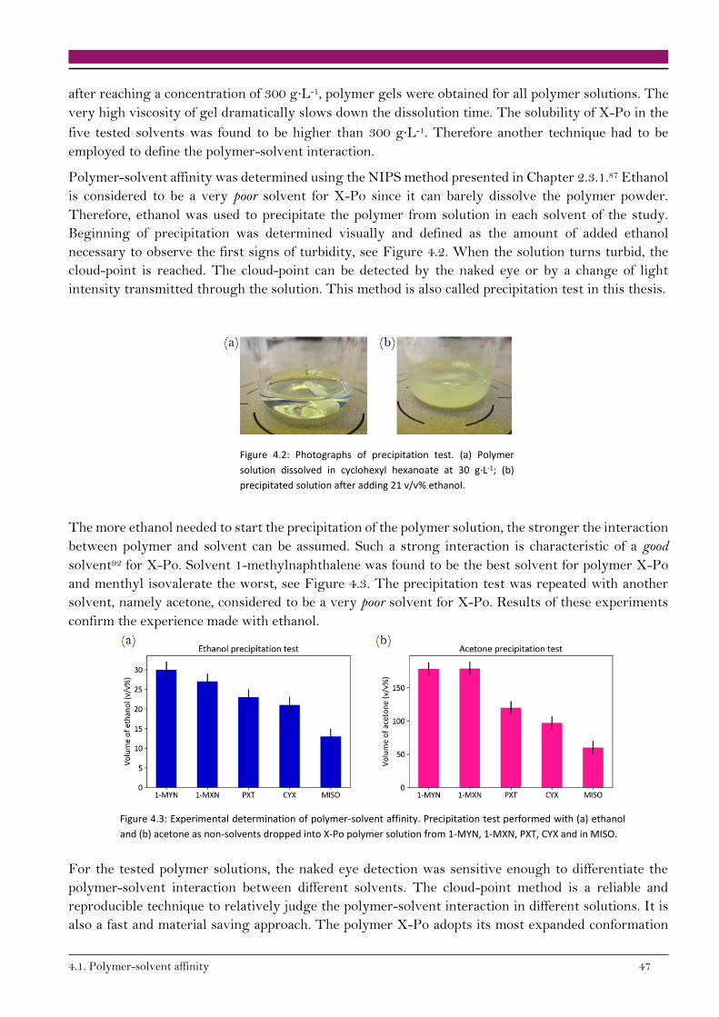
4.1. Polymer-solvent affinity 47
after reaching a concentration of 300 g∙L-1, polymer gels were obtained for all polymer solutions. The
very high viscosity of gel dramatically slows down the dissolution time. The solubility of X-Po in the
five tested solvents was found to be higher than 300 g∙L-1. Therefore another technique had to be
employed to define the polymer-solvent interaction.
Polymer-solvent affinity was determined using the NIPS method presented in Chapter 2.3.1.87 Ethanol
is considered to be a very poor solvent for X-Po since it can barely dissolve the polymer powder.
Therefore, ethanol was used to precipitate the polymer from solution in each solvent of the study.
Beginning of precipitation was determined visually and defined as the amount of added ethanol
necessary to observe the first signs of turbidity, see Figure 4.2. When the solution turns turbid, the
cloud-point is reached. The cloud-point can be detected by the naked eye or by a change of light
intensity transmitted through the solution. This method is also called precipitation test in this thesis.
Figure 4.2: Photographs of precipitation test. (a) Polymer
solution dissolved in cyclohexyl hexanoate at 30 g∙L-1; (b)
precipitated solution after adding 21 v/v% ethanol.
The more ethanol needed to start the precipitation of the polymer solution, the stronger the interaction
between polymer and solvent can be assumed. Such a strong interaction is characteristic of a good
solvent92 for X-Po. Solvent 1-methylnaphthalene was found to be the best solvent for polymer X-Po
and menthyl isovalerate the worst, see Figure 4.3. The precipitation test was repeated with another
solvent, namely acetone, considered to be a very poor solvent for X-Po. Results of these experiments
confirm the experience made with ethanol.
Figure 4.3: Experimental determination of polymer-solvent affinity. Precipitation test performed with (a) ethanol
and (b) acetone as non-solvents dropped into X-Po polymer solution from 1-MYN, 1-MXN, PXT, CYX and in MISO.
For the tested polymer solutions, the naked eye detection was sensitive enough to differentiate the
polymer-solvent interaction between different solvents. The cloud-point method is a reliable and
reproducible technique to relatively judge the polymer-solvent interaction in different solutions. It is
also a fast and material saving approach. The polymer X-Po adopts its most expanded conformation
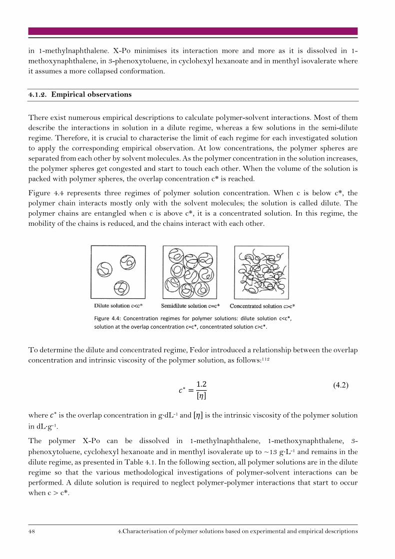
48 4.Characterisation of polymer solutions based on experimental and empirical descriptions
in 1-methylnaphthalene. X-Po minimises its interaction more and more as it is dissolved in 1-
methoxynaphthalene, in 3-phenoxytoluene, in cyclohexyl hexanoate and in menthyl isovalerate where
it assumes a more collapsed conformation.
4.1.2. Empirical observations
There exist numerous empirical descriptions to calculate polymer-solvent interactions. Most of them
describe the interactions in solution in a dilute regime, whereas a few solutions in the semi-dilute
regime. Therefore, it is crucial to characterise the limit of each regime for each investigated solution
to apply the corresponding empirical observation. At low concentrations, the polymer spheres are
separated from each other by solvent molecules. As the polymer concentration in the solution increases,
the polymer spheres get congested and start to touch each other. When the volume of the solution is
packed with polymer spheres, the overlap concentration c* is reached.
Figure 4.4 represents three regimes of polymer solution concentration. When c is below c*, the
polymer chain interacts mostly only with the solvent molecules; the solution is called dilute. The
polymer chains are entangled when c is above c*, it is a concentrated solution. In this regime, the
mobility of the chains is reduced, and the chains interact with each other.
Figure 4.4: Concentration regimes for polymer solutions: dilute solution c<c*,
solution at the overlap concentration c=c*, concentrated solution c>c*.
To determine the dilute and concentrated regime, Fedor introduced a relationship between the overlap
concentration and intrinsic viscosity of the polymer solution, as follows:112
𝑐∗ =
1.2
[𝜂]
(4.2)
where 𝑐∗ is the overlap concentration in g∙dL-1 and [𝜂] is the intrinsic viscosity of the polymer solution
in dL∙g-1.
The polymer X-Po can be dissolved in 1-methylnaphthalene, 1-methoxynaphthalene, 3-
phenoxytoluene, cyclohexyl hexanoate and in menthyl isovalerate up to ~13 g∙L-1 and remains in the
dilute regime, as presented in Table 4.1. In the following section, all polymer solutions are in the dilute
regime so that the various methodological investigations of polymer-solvent interactions can be
performed. A dilute solution is required to neglect polymer-polymer interactions that start to occur
when c > c*.
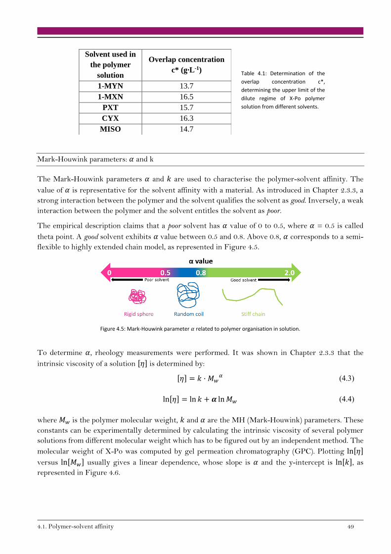
4.1. Polymer-solvent affinity 49
Solvent used in
the polymer
solution
Overlap concentration
c* (g∙L-1)
1-MYN 13.7 1-MXN 16.5
PXT 15.7 CYX 16.3 MISO 14.7
Table 4.1: Determination of the
overlap concentration c*,
determining the upper limit of the
dilute regime of X-Po polymer
solution from different solvents.
Mark-Houwink parameters: 𝛼 and k
The Mark-Houwink parameters 𝛼 and 𝑘 are used to characterise the polymer-solvent affinity. The
value of 𝛼 is representative for the solvent affinity with a material. As introduced in Chapter 2.3.3, a
strong interaction between the polymer and the solvent qualifies the solvent as good. Inversely, a weak
interaction between the polymer and the solvent entitles the solvent as poor.
The empirical description claims that a poor solvent has 𝛼 value of 0 to 0.5, where 𝛼 = 0.5 is called
theta point. A good solvent exhibits 𝛼 value between 0.5 and 0.8. Above 0.8, 𝛼 corresponds to a semi-
flexible to highly extended chain model, as represented in Figure 4.5.
Figure 4.5: Mark-Houwink parameter 𝛼 related to polymer organisation in solution.
To determine 𝛼, rheology measurements were performed. It was shown in Chapter 2.3.3 that the
intrinsic viscosity of a solution [𝜂] is determined by:
[𝜂] = 𝑘 · 𝑀𝑤𝛼 (4.3)
ln[𝜂] = ln 𝑘 + 𝜶 ln 𝑀𝑤 (4.4)
where 𝑀𝑤 is the polymer molecular weight, 𝑘 and 𝛼 are the MH (Mark-Houwink) parameters. These
constants can be experimentally determined by calculating the intrinsic viscosity of several polymer
solutions from different molecular weight which has to be figured out by an independent method. The
molecular weight of X-Po was computed by gel permeation chromatography (GPC). Plotting ln[𝜂]
versus ln[𝑀𝑤] usually gives a linear dependence, whose slope is 𝛼 and the y-intercept is ln[𝑘], as
represented in Figure 4.6.
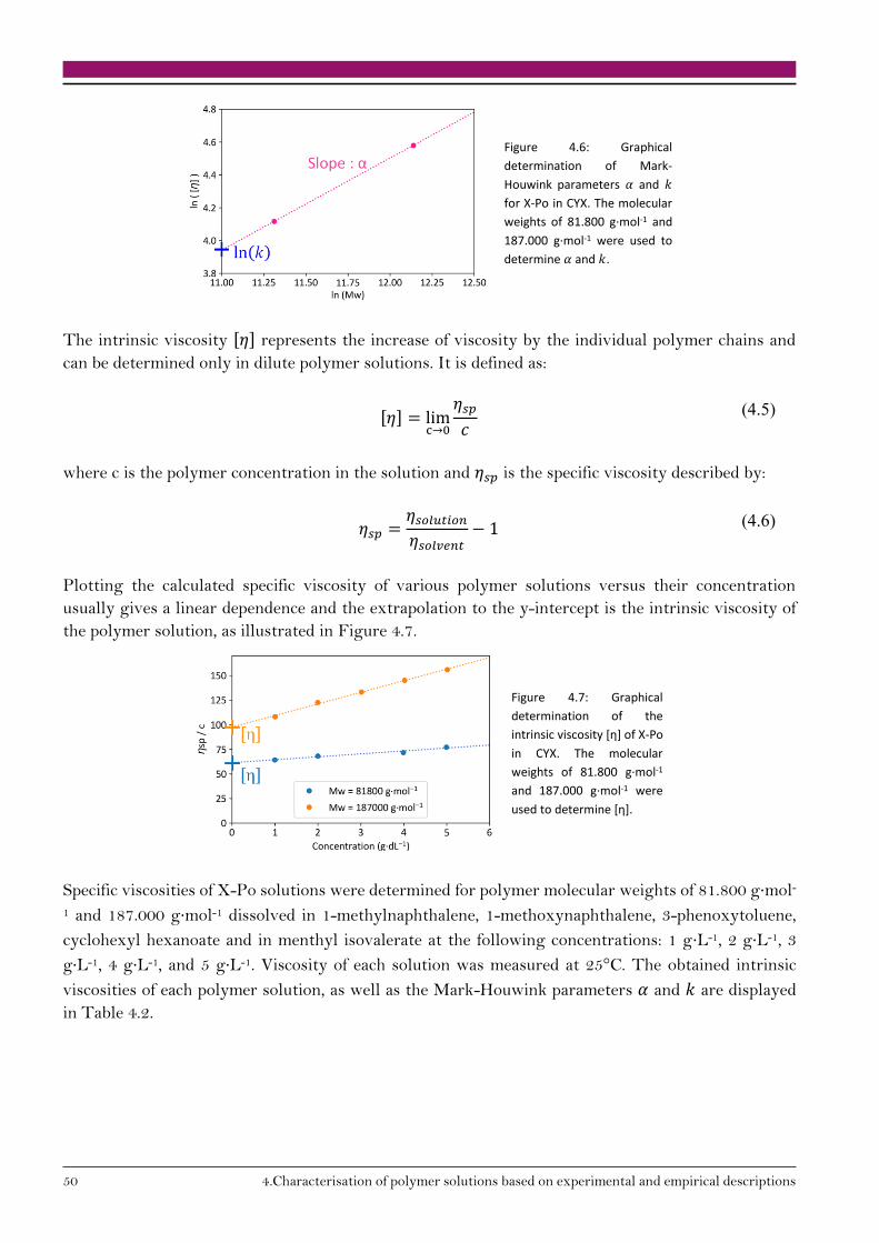
50 4.Characterisation of polymer solutions based on experimental and empirical descriptions
Figure 4.6: Graphical
determination of Mark-
Houwink parameters 𝛼 and 𝑘
for X-Po in CYX. The molecular
weights of 81.800 g·mol-1 and
187.000 g·mol-1 were used to
determine 𝛼 and 𝑘.
The intrinsic viscosity [𝜂] represents the increase of viscosity by the individual polymer chains and
can be determined only in dilute polymer solutions. It is defined as:
[𝜂] = limc→0
𝜂𝑠𝑝
𝑐
(4.5)
where c is the polymer concentration in the solution and 𝜂𝑠𝑝 is the specific viscosity described by:
𝜂𝑠𝑝 =𝜂𝑠𝑜𝑙𝑢𝑡𝑖𝑜𝑛
𝜂𝑠𝑜𝑙𝑣𝑒𝑛𝑡− 1 (4.6)
Plotting the calculated specific viscosity of various polymer solutions versus their concentration
usually gives a linear dependence and the extrapolation to the y-intercept is the intrinsic viscosity of
the polymer solution, as illustrated in Figure 4.7.
Figure 4.7: Graphical
determination of the
intrinsic viscosity [η] of X-Po
in CYX. The molecular
weights of 81.800 g·mol-1
and 187.000 g·mol-1 were
used to determine [η].
Specific viscosities of X-Po solutions were determined for polymer molecular weights of 81.800 g∙mol-
1 and 187.000 g∙mol-1 dissolved in 1-methylnaphthalene, 1-methoxynaphthalene, 3-phenoxytoluene,
cyclohexyl hexanoate and in menthyl isovalerate at the following concentrations: 1 g∙L-1, 2 g∙L-1, 3
g∙L-1, 4 g∙L-1, and 5 g∙L-1. Viscosity of each solution was measured at 25°C. The obtained intrinsic
viscosities of each polymer solution, as well as the Mark-Houwink parameters 𝛼 and 𝑘 are displayed
in Table 4.2.
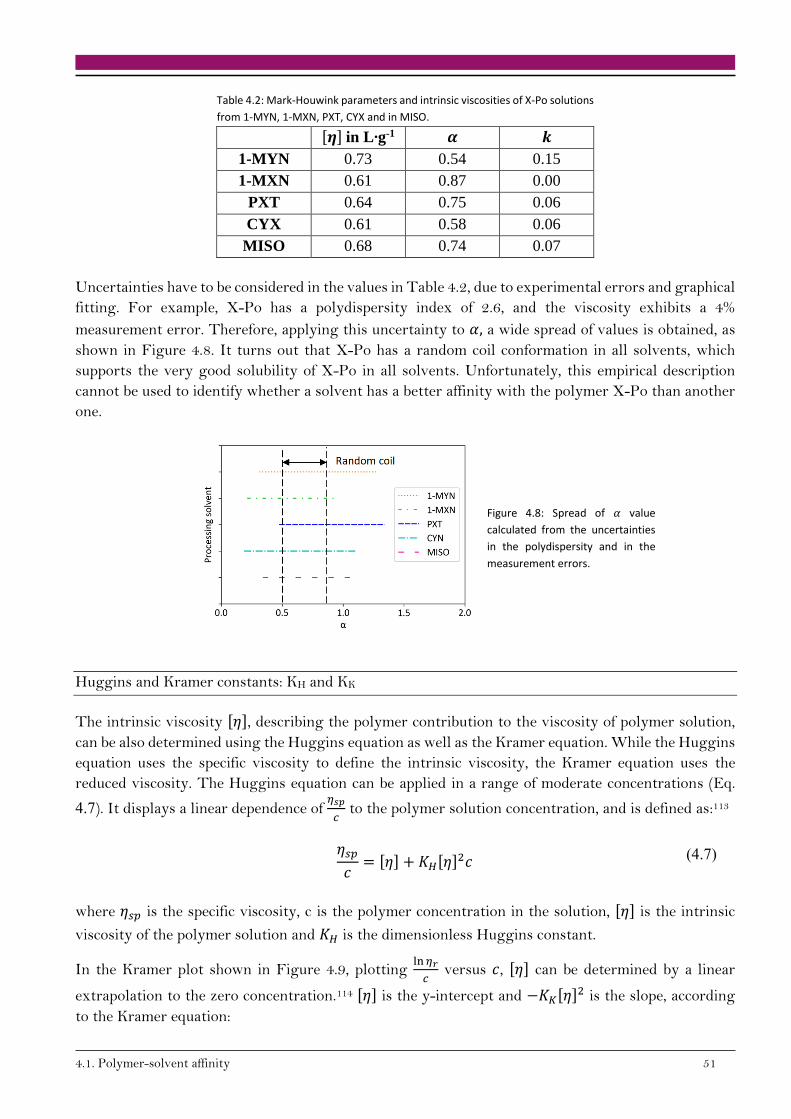
4.1. Polymer-solvent affinity 51
Table 4.2: Mark-Houwink parameters and intrinsic viscosities of X-Po solutions
from 1-MYN, 1-MXN, PXT, CYX and in MISO.
[𝜼] in L∙g-1 𝜶 𝒌
1-MYN 0.73 0.54 0.15
1-MXN 0.61 0.87 0.00
PXT 0.64 0.75 0.06
CYX 0.61 0.58 0.06
MISO 0.68 0.74 0.07
Uncertainties have to be considered in the values in Table 4.2, due to experimental errors and graphical
fitting. For example, X-Po has a polydispersity index of 2.6, and the viscosity exhibits a 4%
measurement error. Therefore, applying this uncertainty to 𝛼, a wide spread of values is obtained, as
shown in Figure 4.8. It turns out that X-Po has a random coil conformation in all solvents, which
supports the very good solubility of X-Po in all solvents. Unfortunately, this empirical description
cannot be used to identify whether a solvent has a better affinity with the polymer X-Po than another
one.
Figure 4.8: Spread of 𝛼 value
calculated from the uncertainties
in the polydispersity and in the
measurement errors.
Huggins and Kramer constants: KH and KK
The intrinsic viscosity [𝜂], describing the polymer contribution to the viscosity of polymer solution,
can be also determined using the Huggins equation as well as the Kramer equation. While the Huggins
equation uses the specific viscosity to define the intrinsic viscosity, the Kramer equation uses the
reduced viscosity. The Huggins equation can be applied in a range of moderate concentrations (Eq.
4.7). It displays a linear dependence of 𝜂𝑠𝑝
𝑐 to the polymer solution concentration, and is defined as:113
𝜂𝑠𝑝
𝑐= [𝜂] + 𝐾𝐻[𝜂]2𝑐
(4.7)
where 𝜂𝑠𝑝 is the specific viscosity, c is the polymer concentration in the solution, [𝜂] is the intrinsic
viscosity of the polymer solution and 𝐾𝐻 is the dimensionless Huggins constant.
In the Kramer plot shown in Figure 4.9, plotting ln 𝜂𝑟
𝑐 versus 𝑐, [𝜂] can be determined by a linear
extrapolation to the zero concentration.114 [𝜂] is the y-intercept and −𝐾𝐾[𝜂]2 is the slope, according
to the Kramer equation:
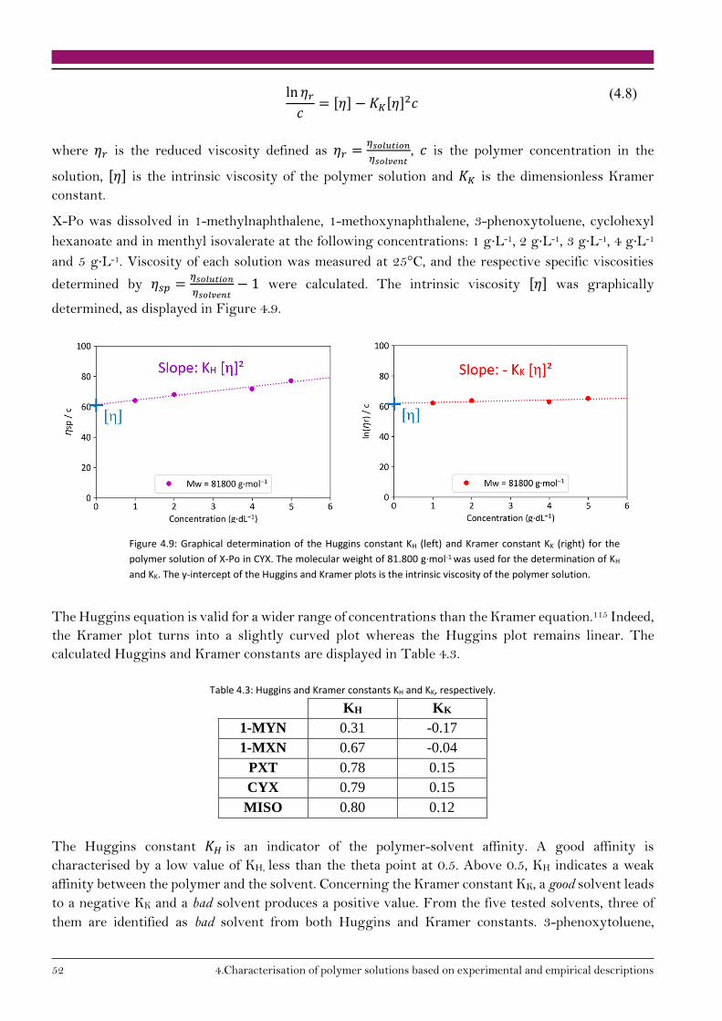
52 4.Characterisation of polymer solutions based on experimental and empirical descriptions
ln 𝜂𝑟
𝑐= [𝜂] − 𝐾𝐾[𝜂]2𝑐
(4.8)
where 𝜂𝑟 is the reduced viscosity defined as 𝜂𝑟 =𝜂𝑠𝑜𝑙𝑢𝑡𝑖𝑜𝑛
𝜂𝑠𝑜𝑙𝑣𝑒𝑛𝑡, 𝑐 is the polymer concentration in the
solution, [𝜂] is the intrinsic viscosity of the polymer solution and 𝐾𝐾 is the dimensionless Kramer
constant.
X-Po was dissolved in 1-methylnaphthalene, 1-methoxynaphthalene, 3-phenoxytoluene, cyclohexyl
hexanoate and in menthyl isovalerate at the following concentrations: 1 g∙L-1, 2 g∙L-1, 3 g∙L-1, 4 g∙L-1
and 5 g∙L-1. Viscosity of each solution was measured at 25°C, and the respective specific viscosities
determined by 𝜂𝑠𝑝 =𝜂𝑠𝑜𝑙𝑢𝑡𝑖𝑜𝑛
𝜂𝑠𝑜𝑙𝑣𝑒𝑛𝑡− 1 were calculated. The intrinsic viscosity [𝜂] was graphically
determined, as displayed in Figure 4.9.
Figure 4.9: Graphical determination of the Huggins constant KH (left) and Kramer constant KK (right) for the
polymer solution of X-Po in CYX. The molecular weight of 81.800 g·mol-1 was used for the determination of KH
and KK. The y-intercept of the Huggins and Kramer plots is the intrinsic viscosity of the polymer solution.
The Huggins equation is valid for a wider range of concentrations than the Kramer equation.115 Indeed,
the Kramer plot turns into a slightly curved plot whereas the Huggins plot remains linear. The
calculated Huggins and Kramer constants are displayed in Table 4.3.
Table 4.3: Huggins and Kramer constants KH and KK, respectively.
KH KK
1-MYN 0.31 -0.17
1-MXN 0.67 -0.04
PXT 0.78 0.15
CYX 0.79 0.15
MISO 0.80 0.12
The Huggins constant 𝐾𝐻 is an indicator of the polymer-solvent affinity. A good affinity is
characterised by a low value of KH, less than the theta point at 0.5. Above 0.5, KH indicates a weak
affinity between the polymer and the solvent. Concerning the Kramer constant KK, a good solvent leads
to a negative KK and a bad solvent produces a positive value. From the five tested solvents, three of
them are identified as bad solvent from both Huggins and Kramer constants. 3-phenoxytoluene,

4.1. Polymer-solvent affinity 53
cyclohexyl hexanoate and menthyl isovalerate are having a weak interaction with polymer X-Po. The
solvent 1-methoxynaphthalene is close to the theta point. On the other hand, 1-methylnaphthalene is
considered as a good solvent.
Both Huggins and Kramer equations can be plotted on the same graph to identify whether the curves
meet at the concentration 𝑐 = 0, as in Figure 4.10. It is an indicator of whether the calculations and
the intrinsic viscosity determinations are meaningful. For the five X-Po tested solutions, Huggins and
Kramer representations coincide at concentration 𝑐 = 0. Therefore, the intrinsic viscosities
determined by both equations are similar and are meaningful. Kramer and Huggins constants are useful
to identify whether a solvent exhibits a stronger affinity to a given material than another one.
Figure 4.10: Determination of intrinsic
viscosity by Huggins and Kramer equations of
X-Po solutions from (a) 1-MYN, (b) 1-MXN, (c)
PXT, (d) CYX and (e) MISO. The intrinsic
viscosity is the viscosity of the polymer
solution at concentration zero.
54 4.Characterisation of polymer solutions based on experimental and empirical descriptions
Solomon Ciuta equation: single point determination
At low polymer solution concentration, it can be assumed that both Huggins and Kramer equations
are linear, as shown in Figure 4.10. Solomon Ciuta developed an empirical observation using a single
point to determine the intrinsic viscosity of a polymer solution, stating that:116
[𝜂] =√2(𝜂𝑠𝑝 − ln 𝜂𝑟)
𝑐=
√2(𝜂𝑟 − 1 − ln 𝜂𝑟)
𝑐
(4.9)
where [𝜂] is the intrinsic viscosity of the polymer solution, 𝜂𝑠𝑝 is the specific viscosity determined by
𝜂𝑠𝑝 =𝜂𝑠𝑜𝑙𝑢𝑡𝑖𝑜𝑛
𝜂𝑠𝑜𝑙𝑣𝑒𝑛𝑡− 1, 𝜂𝑟 is the reduced viscosity defined as 𝜂𝑟 =
𝜂𝑠𝑜𝑙𝑢𝑡𝑖𝑜𝑛
𝜂𝑠𝑜𝑙𝑣𝑒𝑛𝑡, and 𝑐 is the polymer concen-
tration in the solution.
The Solomon Ciuta equation is valid only when the linear Huggins and Kraemer equations are both
valid.115 To perform the intrinsic viscosity evaluation, a polymer solution of X-Po at 0.1 g∙L-1 was
employed. The intrinsic viscosity of X-Po in 1-methylnaphthalene, in 1-methoxynaphthalene, in 3-
phenoxytoluene, in cyclohexyl hexanoate and in menthyl isovalerate resolved by Solomon Ciuta
equation are displayed in Table 4.4. A comparison of the intrinsic viscosities of the same polymer
solutions determined by Mark-Houwink, Huggins and Kramer equations are also displayed.
Table 4.4: Intrinsic viscosities determined from Mark-Houwink equation, Huggins equation, Kramer equation and Solomon Ciuta
equation.
Intrinsic viscosity in L∙g-1
From Mark-
Houwink equation
From Huggins
equation
From Kramer
equation
From Solomon
Ciuta equation
1-MYN 0.73 0.73 0.73 0.74
1-MXN 0.61 0.61 0.62 0.64
PXT 0.64 0.64 0.64 0.66
CYX 0.61 0.61 0.61 0.65
MISO 0.68 0.68 0.69 0.72
In a very dilute polymer solution, the viscosity is defined as the viscosity of the pure solvent plus the
contribution of the individual polymer chains. The intrinsic viscosity of a polymer solution describes
the hydrodynamic volume of a polymer chain in a given solvent. Therefore, this measure gives an
understanding of the polymer-solvent interaction. A low intrinsic viscosity is related to a small radius
of gyration 𝑅𝑔 and is obtained for a polymer in a poor solvent. Oppositely, a good solvent favours the
polymer-solvent interaction resulting in a higher intrinsic viscosity.117
Mark-Houwink, Huggins, Kramer and Solomon Ciuta equations provide similar intrinsic viscosity
values for polymer X-Po in 1-methylnaphthalene, in 1-methoxynaphthalene, in 3-phenoxytoluene, in
cyclohexyl hexanoate and in menthyl isovalerate. The values are between 0.61 and 0.74 L∙g-1. The
polymer X-Po has comparable intrinsic viscosities in all tested solvents and therefore hinders the
identification of a preferred interaction of X-Po with a specific solvent. The Mark-Houwink and
Solomon Ciuta equations cannot distinguish the difference in polymer-solvent interactions of the
4.2. Polymer size in solution 55
investigated polymer solutions. However, the Huggins and the Kraemer constants identified disparities
in the different polymer solutions. 1-methynaphthalene is found to exhibit the strongest interaction
with X-Po, which correlates with the result obtained by the precipitation test in Chapter 4.1.1. Huggins
and Kraemer constants also classified 3-phenoxytoluene, cyclohexyl hexanoate and menthyl
isovalerate as poor solvents for X-Po. However, no differentiation of affinity is possible between the
three solvents. Nevertheless, the trend obtained by Huggins and Kraemer constants goes along with
the experimental measurements of the polymer-solvent interactions classifying the ink solvent from
the better to the worse solvent as: 1-methylnaphthalene, 1-methoxynaphthalene, 3-phenoxytoluene,
cyclohexyl hexanoate and menthyl isovalerate. This goes along with the apparently decreasing
hydrophobicity of the solvents judged by the oxygen content of the solvents, as seen from Table 3.3.
4.2. Polymer size in solution
The size of a polymer chain in a solvent is directly related to the interaction of the polymer with the
solvent molecules as detailed in Chapter 2.3.2. In this section, polymer size in solution was
characterised by its radius of gyration 𝑅𝑔 determined from Flory and Fox equation and by its volume
fraction from Einstein equation.
Experimentally, the size of polymer in solution can be determined by various methods. Dynamic light
scattering (DLS) and ultrasonic attenuation spectroscopy (UAS) are two widely used techniques. DLS,
also called photon correlation spectroscopy, measures scattering intensity fluctuation over time of light
passing through a solution. The fluctuations characterise the Brownian motion within the sample.
These fluctuations are used to calculate the hydrodynamic radius Rh. On the other side, UAS applies
plane sound waves moving through a solution. The attenuated wave is collected in a receiver and the
size of polymer in solution is calculated. However, UAS suffers from a low resolution and the
mathematical model requires intense data evaluation. Therefore, DLS was chosen to experimentally
determine the polymer size in the tested solvents.
4.2.1. Radius of gyration
The size of a polymer in solution is defined by its radius of gyration described by 𝑅𝑔 as in Figure 4.11.
Figure 4.11: Radius of gyration 𝑅𝑔
of a random coil polymer in
solution.
In a good solvent, the polymer coil tends to expand, thus the radius of gyration of the polymer is bigger
than the one of the same polymer in a poor solvent. The radius of gyration can be estimated by the
Flory and Fox equation,118 stating that:
[𝜂] = 𝛷′ · 𝑅𝑔3 · 𝑀−1 (4.10)
or
56 4.Characterisation of polymer solutions based on experimental and empirical descriptions
𝑅𝑔 = √([𝜂]
𝛷′· 𝑀𝑤)
3
(4.11)
where [𝜂] is the intrinsic viscosity in L∙g-1, 𝑅𝑔 is the radius of gyration in m, 𝛷′ = 2.1 x 1026 kmol-1 is
a universal constant independent of temperature and polymer-solvent system117 and 𝑀𝑤 is the
molecular weight of the polymer in g∙kmol-1. The molecular weight can be calculated from the intrinsic
viscosity of the polymer solution, determined in Chapter 3.1.4, utilising the Mark-Houwink parameters
𝛼 and 𝑘,119 as introduced in Chapter 2.3.3, by:
[𝜂] = 𝑘 · 𝑀𝑤𝛼 (4.12)
or
𝑀𝑤 = √([𝜂]
𝑘)
𝛼
(4.13)
The radii of gyration calculated for the polymer X-Po in 1-methylnaphthalene, 1-methoxynaphthalene,
3-phenoxytoluene, cyclohexyl hexanoate and in menthyl isovalerate are approximately equal to 1 nm
and are displayed in Table 4.5. Taking into account the error carried by the Mark-Houwink parameters
used to calculate the polymer molecular weight, and the error generated by the graphical determination
of the intrinsic viscosity, it can be considered that the calculated radius of gyration of X-Po is similar
in all tested solvents. Flory and Fox equation indicates that the diverse polymer sizes in the tested
polymer solutions cannot be distinguished. To further investigate the polymer size in solution, the X-
Po volume fraction will be determined by the Einstein equation supported by viscosity measurements.
In addition, the polymer diameter in solution will be directly measured by dynamic light scattering
where no calculation error is included.
Table 4.5: Radius of gyration of X-Po in the different solvents calculated by Flory
and Fox equation.
Solvents
Calculated
molecular weight
(g∙kmol-1)
Radius gyration
(nm)
1-MYN 0.25273 0.5
1-MXN 30.14789 2.1
PXT 8.24511 1.4
CYX 0.53422 0.5
MISO 7.35939 1.3
4.2.2. Volume fraction
In 1945, Einstein established a relationship between the volume fraction 𝛷 of suspended material and
𝜂 the viscosity of the suspension. 120 For a sphere or a random coil, the equation is:
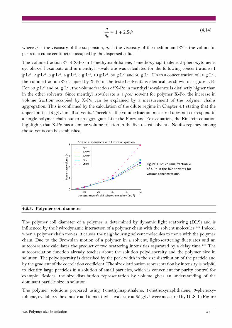
4.2. Polymer size in solution 57
𝜂
𝜂𝑠= 1 + 2.5𝛷 (4.14)
where 𝜂 is the viscosity of the suspension, 𝜂𝑠 is the viscosity of the medium and 𝛷 is the volume in
parts of a cubic centimetre occupied by the dispersed solid.
The volume fraction 𝛷 of X-Po in 1-methylnaphthalene, 1-methoxynaphthalene, 3-phenoxytoluene,
cyclohexyl hexanoate and in menthyl isovalerate was calculated for the following concentrations: 1
g∙L-1, 2 g∙L-1, 3 g∙L-1, 4 g∙L-1, 5 g∙L-1, 10 g∙L-1, 30 g∙L-1 and 50 g∙L-1. Up to a concentration of 10 g∙L-1,
the volume fraction 𝛷 occupied by X-Po in the tested solvents is identical, as shown in Figure 4.12.
For 30 g∙L-1 and 50 g∙L-1, the volume fraction of X-Po in menthyl isovalerate is distinctly higher than
in the other solvents. Since menthyl isovalerate is a poor solvent for polymer X-Po, the increase in
volume fraction occupied by X-Po can be explained by a measurement of the polymer chains
aggregation. This is confirmed by the calculation of the dilute regime in Chapter 4.1 stating that the
upper limit is 13 g∙L-1 in all solvents. Therefore, the volume fraction measured does not correspond to
a single polymer chain but to an aggregate. Like the Flory and Fox equation, the Einstein equation
highlights that X-Po has a similar volume fraction in the five tested solvents. No discrepancy among
the solvents can be established.
Figure 4.12: Volume fraction 𝛷
of X-Po in the five solvents for
various concentrations.
4.2.3. Polymer coil diameter
The polymer coil diameter of a polymer is determined by dynamic light scattering (DLS) and is
influenced by the hydrodynamic interaction of a polymer chain with the solvent molecules.121 Indeed,
when a polymer chain moves, it causes the neighbouring solvent molecules to move with the polymer
chain. Due to the Brownian motion of a polymer in a solvent, light-scattering fluctuates and an
autocorrelator calculates the product of two scattering intensities separated by a delay time.122 The
autocorrelation function already teaches about the solution polydispersity and the polymer size in
solution. The polydispersity is described by the peak width in the size distribution of the particle and
by the gradient of the correlation coefficient. The size distribution representation by intensity is helpful
to identify large particles in a solution of small particles, which is convenient for purity control for
example. Besides, the size distribution representation by volume gives an understanding of the
dominant particle size in solution.
The polymer solutions prepared using 1-methylnaphthalene, 1-methoxynaphthalene, 3-phenoxy-
toluene, cyclohexyl hexanoate and in menthyl isovalerate at 50 g∙L-1 were measured by DLS. In Figure

58 4.Characterisation of polymer solutions based on experimental and empirical descriptions
4.13 X-Po has a similar coil diameter of less than 1 nm in all tested solvents except in menthyl
isovalerate where the peak is shifted to slightly larger size of roughly 1.7 nm. Malvern proclaims a
measurement sensitivity down to 0.3 nm.123 The measured X-Po diameter in the five tested solvents
can be considered equal taking into account that these values are close to the detection limit. A
concentration of 50 g∙L-1 was required to get enough scattering, i.e., enough light intensity on the
detector. However, at that concentration the polymer solutions are not in the dilute regime anymore.
Therefore, the DLS measurements report the size of polymer aggregates. This is in agreement with
the size in suspension obtained by the Einstein equation in Chapter 4.2.2.
Figure 4.13: Size distribution of X-Po in all solvents represented by (a) intensity and (b) volume.
Measuring DLS of less concentrated polymer solutions would give the coil diameter of single polymer
chains and not of an aggregate. However, X-Po met measurement limitations at low solution
concentration since no signal could be detected. To get around this limitation, polymer X-Po should
be investigated by DLS for a polymer with a higher molecular weight. The coiled single polymer chain
would then be larger, would scatter more and there would be enough light to be detected, even at low
concentrations.
4.3. Conclusion on polymer solution characterisation
In this chapter, the affinity of X-Po polymer with the ink solvents was investigated to characterise the
polymer solutions made from 1-methynaphthalene, 1-methoxynaphthalene, 3-phenoxytoluene,
cyclohexyl hexanoate and from menthyl isovalerate. The study was based on experimental
measurements and empirical descriptions. The affinity of a polymer with a solvent indicates the
intensity of interaction or binding occurring between the polymer chains and the solvent molecules. A
solvent exhibiting a low interaction with a polymer is called a poor solvent and leads to enhanced
intramolecular interactions resulting in a decrease of the radius of gyration 𝑅𝑔. On the opposite, in a
good solvent, the polymer chains expand and tend to maximise their contact with the solvent molecules,
resulting in a larger radius of gyration.
The polymer-solvent interaction is directly proportional to the polymer solubility in the solvent by the
Hildebrand-Scott equation.124 Thus, the solubility of a polymer in a solvent describes their interaction.
To investigate the solubility of X-Po in the five solvents, the Non-solvent Induced Phase Separation

4.3. Conclusion on polymer solution characterisation 59
(NIPS) technique was performed by the use of the cloud-point determination. A non-solvent was added
in the polymer solution dropwise until the solution turned turbid. Ethanol and acetone were tested as
they are very poor solvents for X-Po. The more poor solvent needed to start the precipitation of the
polymer solution, the stronger is the interaction between polymer and solvent. X-Po minimises its
interaction more and more as it is dissolved in 1-methynaphthalene, in 1-methoxynaphthalene, in 3-
phenoxytoluene, in cyclohexyl hexanoate and in menthyl isovalerate where it assumes a more collapsed
conformation. The NIPS technique is a fast and material saving approach to judge the polymer-solvent
interaction in different solutions.
An empirical observation was used to also characterise the polymer X-Po interaction with the five
solvents. Most of the empirical descriptions investigate polymer solutions in the dilute regime. Fedor
introduced a relationship between the overlap concentration c* and the intrinsic viscosity [𝜂] of the
polymer solution, defined in Chapter 2.3.3. Mark-Houwink presented the parameters 𝛼 and 𝑘, where
𝛼 describes the polymer-solvent affinity. A poor solvent has 𝛼 value from 0 to 0.5, a good solvent from
0.5 to 0.8, where 0.5 is the theta point. Above 0.8, 𝛼 indicates that the polymer adopts an extended
chain conformation. The determination of 𝛼 is conducted graphically as well as the intrinsic viscosity,
which describes the polymer contribution to the viscosity of the polymer solution. It turns out that X-
Po has a random coil conformation in all solvents, which supports the very good solubility of X-Po in
all solvents. Unfortunately, 𝛼 cannot be used to distinguish between the solvents affinity with polymer
X-Po. The intrinsic viscosity can also be determined using the Huggins and Kramer equations,
introducing the constants 𝐾𝐻 and 𝐾𝐾, respectively. While the Huggins equation uses the specific
viscosity to define the intrinsic viscosity, the Kramer equation uses the reduced viscosity 𝜂𝑟. A good
affinity is characterised by a low value of KH, less than the theta point at 0.5. Above 0.5, KH indicates a
week affinity between the polymer and the solvent. Concerning the Kramer constant KK, a good solvent
leads to a negative KK and a bad solvent produces a positive KK. The Huggins and Kramer constants
identified 3-phenoxytoluene, cyclohexyl hexanoate and menthyl isovalerate as solvents exhibiting the
weakest interaction with X-Po, whereas 1-methoxynaphthalene is close to a theta solvent and 1-
methylnaphthalene is considered as a good solvent for X-Po. At low polymer solution concentration,
Solomon Ciuta developed an empirical observation with a single point to determine the intrinsic
viscosity of a polymer solution using the reduced viscosity at one very low concentration. A low
intrinsic viscosity is related to a small radius of gyration 𝑅𝑔 and is obtained for a polymer in a poor
solvent. Oppositely, a good solvent favours the polymer-solvent interaction resulting in a higher
intrinsic viscosity. However, the intrinsic viscosities of the polymer solutions fall between 0.61 L∙g-1
and 0.74 L∙g-1 which are very similar. Thus one cannot distinguish the difference in polymer-solvent
interactions of the investigated polymer solutions.
The size of the polymer X-Po in the solvents was then used to understand the interaction of the
polymer with the solvent molecules. The radius of gyration 𝑅𝑔 described by Flory and Fox equation
was calculated with the intrinsic viscosity of the polymer solution, the polymer molecular weight and
an universal constant independent of temperature and the polymer-solvent system given by 𝛷′ = 2.1
x 1026 kmol-1. The radii of gyration calculated for X-Po in the five solvents are of same order of
magnitude. So, the diverse polymer sizes in the tested polymer solutions could not be distinguished by
the Flory and Fox equation.
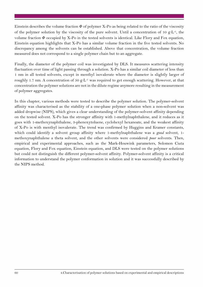
60 4.Characterisation of polymer solutions based on experimental and empirical descriptions
Einstein describes the volume fraction 𝛷 of polymer X-Po as being related to the ratio of the viscosity
of the polymer solution by the viscosity of the pure solvent. Until a concentration of 10 g∙L-1, the
volume fraction 𝛷 occupied by X-Po in the tested solvents is identical. Like Flory and Fox equation,
Einstein equation highlights that X-Po has a similar volume fraction in the five tested solvents. No
discrepancy among the solvents can be established. Above that concentration, the volume fraction
measured does not correspond to a single polymer chain but to an aggregate.
Finally, the diameter of the polymer coil was investigated by DLS. It measures scattering intensity
fluctuation over time of light passing through a solution. X-Po has a similar coil diameter of less than
1 nm in all tested solvents, except in menthyl isovalerate where the diameter is slightly larger of
roughly 1.7 nm. A concentration of 50 g∙L-1 was required to get enough scattering. However, at that
concentration the polymer solutions are not in the dilute regime anymore resulting in the measurement
of polymer aggregates.
In this chapter, various methods were tested to describe the polymer solution. The polymer-solvent
affinity was characterised as the stability of a one-phase polymer solution when a non-solvent was
added dropwise (NIPS), which gives a clear understanding of the polymer-solvent affinity depending
on the tested solvent. X-Po has the stronger affinity with 1-methylnaphthalene, and it reduces as it
goes with 1-methoxynaphthalene, 3-phenoxytoluene, cyclohexyl hexanoate, and the weakest affinity
of X-Po is with menthyl isovalerate. The trend was confirmed by Huggins and Kramer constants,
which could identify a solvent group affinity where 1-methylnaphthalene was a good solvent, 1-
methoxynaphthalene a theta solvent, and the other solvents were considered poor solvents. Then,
empirical and experimental approaches, such as the Mark-Houwink parameters, Solomon Ciuta
equation, Flory and Fox equation, Einstein equation, and DLS were tested on the polymer solutions
but could not distinguish the different polymer-solvent affinity. Polymer-solvent affinity is a critical
information to understand the polymer conformation in solution and it was successfully described by
the NIPS method.
5.1. Cross-linking of X-Po in powder without solvent 61
5. Polymer cross-linking in bulk material and thin films
In this study, the degree of cross-linking of a thin film of a hole transport polymer is presented as a
dependency on the ink formulation. An understanding of the correlation between layer stability and
solvent exposure and the degree of cross-linking in a film was investigated. The degree of cross-linking
of the material is defined by the ratio of the cross-linking reaction enthalpy in film to the cross-linking
reaction enthalpy of the pure powder without solvent, determined by differential scanning calorimetry
(DSC). The layer stability against solvent exposure is determined by the variation of layer topography
induced by a solvent drop left on the layer surface for a given duration. A selection guideline for
promising new ink solvents is discussed.
5.1. Cross-linking of X-Po in powder without solvent
To understand the cross-linking mechanism of the styrene unit contained in the polymer X-Po, it was
first investigated in powder without solvent. The reaction involving two styrene units is described and
followed by infrared spectroscopy (IR). The physical transformation of X-Po during heat treatment
was characterised by DSC.
5.1.1. Styrene cross-linking reaction
IR spectroscopy was used to study the cross-linking process of styrene, the cross-linker unit contained
in X-Po. During cross-linking of the polymer, the styrene signal reduces or disappears.125 A US patent
discloses the resulting species of the cross-linking reaction of two styrene units,126 displayed in Figure
5.1.
Figure 5.1: Resulting
species of the cross-linking
reaction of two styrene
units, disclosed by US
patent from reference.126
G. Klärner et al. described the intensity variations of vibration bands while the styrene cross-linking
reaction occured.127 Considering that only 10% of X-Po monomers contain the styrene cross-linker
unit, the vibration bands corresponding to styrene and the resulting species after cross-linking are
suffering from a weak intensity compared to all other IR vibrations of the polymer chain. Therefore,
the polymer 7X-Po, characterised by 70 % of its monomers containing the styrene unit, was examined
to accentuate the intensity variations of vibration bands during cross-linking. To perform the cross-
linking reaction in powder, 7X-Po and X-Po were treated by a DSC heating ramp from room
temperature to 300°C with a gradient of 20 K∙min-1.
62 5.Polymer cross-linking in bulk material and thin films
Figure 5.2: Infrared spectra of polymer powders of 7X-Po and X-Po before and after cross-linking through
one DSC run from room temperature to 300°C at 20 K·min-1. The spectrum of 7X-Po is displayed in (a) from
850 cm-1 to 1200 cm-1 and in (b) from 1530 cm-1 to 1665 cm-1. The spectrum of X-Po is displayed in (c)
from 850 cm-1 to 1200 cm-1 and in (d) from 1530 cm-1 to 1665 cm-1.
Before heat treatment, the IR spectra of 7X-Po and X-Po samples both exhibit peaks around 905 cm-1
and 990 cm-1 associated to vinyl C-H out-of-plane bending vibrations. These weak bands are
characteristic of the styrene unit. Another peak around 1630 cm-1 is visible before heating and is related
to terminal vinyl C-C stretching absorption. After heating the powders, these three vibration bands
decrease significantly for 7X-Po and disappear for X-Po, see Figure 5.2. New bands emerge after cross-
linking, around 1165 cm-1 and 1175 cm-1, which are affiliated to new C-C stretching vibrations.
In Figure 5.2, the infrared spectrum of Po, the non-cross-linkable version of X-Po is also displayed. It
is a polymer chain without styrene cross-linker and is used as a reference to identify if the cross-linking
reaction results in all styrene units reacted. In the case of X-Po, the cross-linked polymer overlaps with
the Po spectrum around 905 cm-1, 990 cm-1 and 1630 cm-1 indicating that all styrene units reacted. On
the contrary, the spectrum of 7X-Po shows residual vibrations at these bands revealing that the cross-
linking is not completed after the applied DSC heating ramp.
IR spectroscopy is a powerful analysis method to record the cross-linking reaction of styrene units.
However, the signal strength is limited in the case of X-Po due to the low proportion of styrene in the
polymer chain. The larger styrene content of 7X-Po provides a distinct understanding of the styrene
cross-linking reaction. The results support the mechanism discussed in the literature.126

5.1. Cross-linking of X-Po in powder without solvent 63
5.1.2. Cross-linking reaction enthalpy
DSC is a technique measuring the heat capacity of a material or mixture of materials in response to
change of temperature. The sample, in form of powder, film or solution is placed inside a hermetically
sealed aluminium pan. In the heat-flux DSC, the sample pan and the empty reference pan are set on
thermocouples localised inside a furnace which is heated to the desired temperature at a given heating
rate. While the sample and reference pans are heated up through the thermocouples, the heat capacity
of the sample results in a temperature difference between the sample plan and the reference pan. This
difference is measured by the thermocouples and is used to calculate the heat flow by the thermal
equivalent of Ohm’s law:
𝑞 =
∆𝑇
𝑅
(5.1)
where 𝑞 is the sample heat flow, ∆𝑇 is the temperature difference between the sample pan and the
reference pan, and 𝑅 is the thermal conductivity. Since a DSC measurement is running at a constant
pressure, the heat flow is equivalent to an enthalpy change. The difference in heat flow between the
sample and the reference is given by:
∆
𝑑𝐻
𝑑𝑡= (
𝑑𝐻
𝑑𝑡)
𝑠𝑎𝑚𝑝𝑙𝑒− (
𝑑𝐻
𝑑𝑡)
𝑟𝑒𝑓𝑒𝑟𝑒𝑛𝑐𝑒
(5.2)
with (𝑑𝑞
𝑑𝑡)
𝑃=
𝑑𝐻
𝑑𝑡 (5.3)
where 𝐻 is the enthalpy and 𝑑𝐻
𝑑𝑡 is in W∙s-1. In a DSC thermograph, the integral under a peak, above
the baseline, gives the total enthalpy change for a physical transition. A thermogram of polymer
material can reveal various physical reactions, such a glass transition at the temperature 𝑇𝑔,
crystallisation, melting and cross-linking. To render visible specific reactions, the temperature rate
should be carefully chosen. Generally, polymer materials are investigated by a heating rate between
20 K∙min-1 and 50 K∙min-1.
To identify the cross-linking reaction, the pure powders of X-Po and its analogue Po were measured
at a heating rate of 20 K∙min-1. Due to a programmed heating experiment, a change in baseline at the
start-up can be observed in Figure 5.3 (a) and (b) resulting from a difference in the heat capacity of the
sample and the reference. This difference can be explained by a weight discrepancy between the sample
and the reference. The cross-linking reaction was first identified as an exothermic reaction, meaning
heat was released, see Figure 5.3. Indeed, the only difference between Po and X-Po is the presence of
a cross-linker unit. Therefore, the exothermic peak visible in X-Po thermogram is attributed to the
cross-linking reaction at 250°C. By comparing the thermogram of X-Po with its non-cross-linkable
analogue, the glass transition temperature 𝑇𝑔 of the polymers is determined to be 130°C.
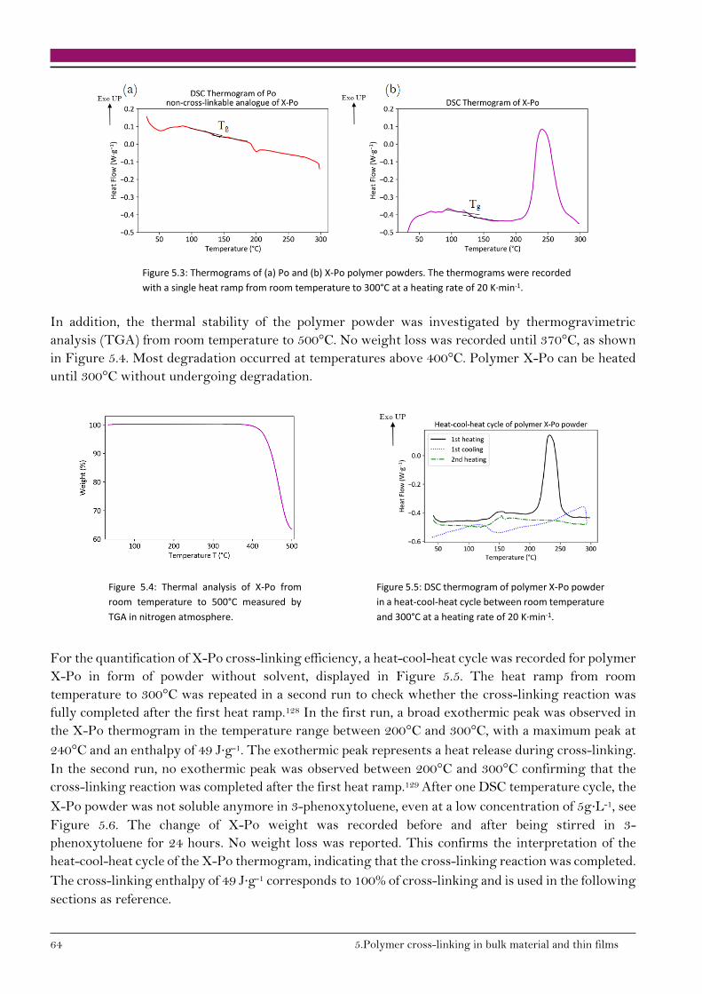
64 5.Polymer cross-linking in bulk material and thin films
Figure 5.3: Thermograms of (a) Po and (b) X-Po polymer powders. The thermograms were recorded
with a single heat ramp from room temperature to 300°C at a heating rate of 20 K∙min-1.
In addition, the thermal stability of the polymer powder was investigated by thermogravimetric
analysis (TGA) from room temperature to 500°C. No weight loss was recorded until 370°C, as shown
in Figure 5.4. Most degradation occurred at temperatures above 400°C. Polymer X-Po can be heated
until 300°C without undergoing degradation.
Figure 5.4: Thermal analysis of X-Po from
room temperature to 500°C measured by
TGA in nitrogen atmosphere.
Figure 5.5: DSC thermogram of polymer X-Po powder
in a heat-cool-heat cycle between room temperature
and 300°C at a heating rate of 20 K∙min-1.
For the quantification of X-Po cross-linking efficiency, a heat-cool-heat cycle was recorded for polymer
X-Po in form of powder without solvent, displayed in Figure 5.5. The heat ramp from room
temperature to 300°C was repeated in a second run to check whether the cross-linking reaction was
fully completed after the first heat ramp.128 In the first run, a broad exothermic peak was observed in
the X-Po thermogram in the temperature range between 200°C and 300°C, with a maximum peak at
240°C and an enthalpy of 49 J∙g-1. The exothermic peak represents a heat release during cross-linking.
In the second run, no exothermic peak was observed between 200°C and 300°C confirming that the
cross-linking reaction was completed after the first heat ramp.129 After one DSC temperature cycle, the
X-Po powder was not soluble anymore in 3-phenoxytoluene, even at a low concentration of 5g∙L-1, see
Figure 5.6. The change of X-Po weight was recorded before and after being stirred in 3-
phenoxytoluene for 24 hours. No weight loss was reported. This confirms the interpretation of the
heat-cool-heat cycle of the X-Po thermogram, indicating that the cross-linking reaction was completed.
The cross-linking enthalpy of 49 J∙g-1 corresponds to 100% of cross-linking and is used in the following
sections as reference.
5.2. Significance of cross-linking in polymer solution 65
Figure 5.6: X-Po powder after undergoing a DSC run in a crucible from
room temperature to 300°C (left) and after being stirred in 3-
phenoxytoluene at a nominal concentration of 5 g∙L-1 for 24 hours (right).
0% ±1% weight loss of the sample was measured after removing the
supernatant of solvent and drying the solid.
5.2. Significance of cross-linking in polymer solution
In this section, the influence of ink solvent on the cross-linking reaction of polymer X-Po is
investigated in more detail. In solution, cross-linker units are surrounded by solvent molecules which
can enhance or reduce the cross-linking efficiency dependent on the polymer conformation in solution.
The hypothesis is that a more collapsed conformation increases the reaction efficiency since the
polymer chains are more attracted to each other than the solvent molecules. To review the cross-
linking in solution, rheology and dynamic light scattering (DLS) measurements were performed.
5.2.1. Rheology investigation
It is well established that polymer molecular weight and chain length increase during cross-linking.130
Increasing the molecular weight of a material having a linear structure is known to increase the
viscosity of a solution.122 Thus, when a polymer starts to cross-link in solution, the viscosity of the
solution will increase.
Viscosity measurements can be performed with various instruments such as capillary, vibrational and
rotational viscometers. The advantage of rotational viscometers is that fluid viscosity is determined as
a function of shear rate by measuring the torque needed to turn an object in a fluid. The dependency
of viscosity regarding shear rate gives an important information especially for the application of inkjet
printing where the ink undergoes extreme shear stress at the jetting step through the nozzle. The
most popular rotational viscometer for viscoelastic fluids is the cone-and-plate geometry.117
Figure 5.7 exhibits the viscosity increase of X-Po solutions which were heat-treated for three hours to
initiate cross-linking in solution. None of the solutions shows an increased viscosity (determined after
cooling at the otherwise same measuring conditions) up to a treatment temperature of 140°C. The
polymer solution prepared using menthyl isovalerate (MISO) cross-links at 170°C. The polymer
solution formulated with cyclohexyl hexanoate (CYX) reveals an increase of viscosity at 170°C, and
cross-links at 180°C. A gradual viscosity increase is observable for the solution from 3-phenoxytoluene
(PXT) up to 7-fold after heat treatment at 200°C. Higher temperatures led to very viscous solutions
that are not measurable with the employed rheometer. The polymer solutions prepared using 1-
methylnaphthalene (1-MYN) and 1-methoxynaphthalene (1-MXN) display a stable viscosity

66 5.Polymer cross-linking in bulk material and thin films
independent of the heat treatment. The most reasonable explanation is that no measurable cross-
linking reaction started in these two solutions.
Figure 5.7: Viscosities polymer
solutions of 50 g∙L-1.measured at room
temperature after heat treatment for
three hours at indicated temperature.
The viscosities are normalised to the
solution viscosity before heat
treatment.
Table 5.1: Photographs of X-Po solutions from cyclohexyl hexanoate and from menthyl isovalerate after a heat treatment of
170°C and 180°C for three hours and cooling down to room temperature.
Solvent used to
prepare the
polymer solution
Treated at 170°C Treated at 180°C
CYX
MISO
The polymer solution prepared using menthyl isovalerate shows a constant viscosity up to a treatment
temperature of 160°C. After a heat treatment of 170°C and 180°C, the polymer solution turns into a
very viscous, jelly-like consistency. The polymer solution prepared using cyclohexyl hexanoate
revealed a 3-fold viscosity after a heat treatment of 170°C. It can be seen in Table 5.1 that the solution
exhibits a solid structure at 180°C.
Using rheology to track the cross-linking reaction of X-Po in solution gives an evident indication of
macroscopic changes and an understanding of the difference between the tested polymer solutions. A
polymer solution prepared using a poor solvent cross-linked at lower temperature than a polymer
5.2. Significance of cross-linking in polymer solution 67
solution prepared using a good solvent. However, no change in viscosity indicates that the degree of
cross-linking is not preeminent enough to impact the viscosity of the solution. To study small cross-
linking phenomenon, DLS was performed since it can detect change in polymer size even in small
volumes.
5.2.2. Variation of species’ size in solution
In order to study the cross-linking reaction in more detail and especially the start of the reaction, DLS
was used to record changes of species size down to the nanometre scale. The polymer solutions were
first measured after being dissolved at 50 g∙L-1 at room temperature and filtered. The polymer
solutions which were heat-treated for three hours at various temperatures to initiate cross-linking were
also measured. The variation of polymer size in solution is an indication that the cross-linking reaction
took place. However, due to optical transmission requirements and viscosity limitations, a choice of
measured solutions had to be made. High viscous solutions could not be measured as well as solutions
whose light absorption interfered with the measurement. The chosen polymer solutions were measured
at 25°C and are displayed in Table 5.2.
Table 5.2: Temperatures applied to the polymer solutions for 3 hours prior to DLS measurements which were
performed at room temperature. The purpose was to identify the progress of cross-linking in solution.
Solvent used to make
the polymer solution
Temperature applied for three hours to the polymer
solutions
1-MYN RT 160°C 200°C
1-MXN RT 160°C 200°C
PXT RT 160°C 180°C
CYX RT 140°C 160°C
MISO RT 140°C 160°C
The size distribution of the polymer solutions measured by DSL can be represented by intensity or by
volume. Both representations lead to different learnings. A minority of large particles can be identified
by an intensity representation of the size distribution. Oppositely, the size distribution representation
by volume gives an understanding of the dominant particle size in solution. In case of a homogeneous
solution of one species size, both intensity and volume will show the same size distribution. However,
if the solution is heterogeneous, one or the other representation will bring different information about
the species. Intensity distribution highlights the presence of large species since they are the ones with
the largest scattering intensity contribution. This is of great interest to identify the cross-linking
progress in solution because even a small amount of cross-linked polymer chains will be visible. If only
a few polymer chains started to cross-link in solution, the volume representation will reveal a high
peak in small species size. In the intensity distribution, these few long chains will be represented by a
peak in the bigger size range. Therefore, both intensity and volume representations are complementary
in the understanding in cross-linking of polymer X-Po in solution.

68 5.Polymer cross-linking in bulk material and thin films
Figure 5.8: Intensity size distribution of X-Po
in (a) 1-methylnaphthalene, (b) 1-
methoxynaphthalene, (c) 3-phenoxytoluene,
(d) cyclohexyl hexanoate, (e) menthyl
isovalerate at a concentration of 50 g∙L-1
measured by DLS after exposure to 140°C
and/or 160°C and/or 180°C and/or 200°C. All
polymer solutions after heat treatment are
measured at 25°C.
From the rheology experiments, no change of viscosity was recorded for the polymer solutions using
1-methylnaphthalene and 1-methoxynaphthalene over the whole tested temperature range. However,
the DLS measurements show that larger size species are appearing when the solution was exposed to
a heat treatment of at least 160°C for all polymer solutions, suggesting that cross-linking of polymer
chains does occur, see Figure 5.8. Being very sensitive to large particles, the intensity representation
does not inform about the proportion of these cross-linked chains relatively to the non-cross-link
counterparts. This is an important information when correlating these results with the rheology
analyses.
From the volume distribution, it becomes obvious that the cross-linked part represents a very small
volume of the overall polymer chains since no peak is visible in the larger species size in the polymer
solutions prepared using 1-methylnaphthalene and 1-methoxynaphthalene, see Figure 5.9. The small
fraction of cross-linked chains highlighted by the volume distribution is in line with the constant
viscosity of both polymer solutions after a heat treatment of 160°C reported in Chapter 5.2.1.
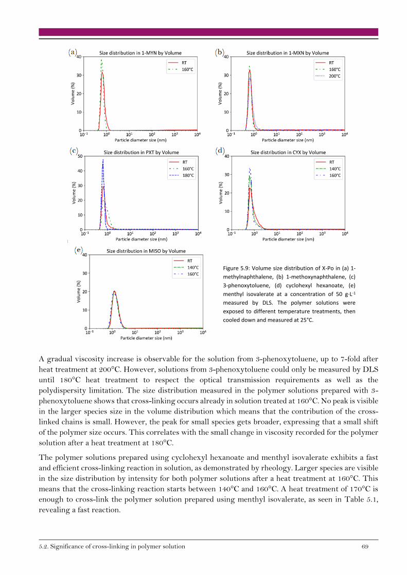
5.2. Significance of cross-linking in polymer solution 69
Figure 5.9: Volume size distribution of X-Po in (a) 1-
methylnaphthalene, (b) 1-methoxynaphthalene, (c)
3-phenoxytoluene, (d) cyclohexyl hexanoate, (e)
menthyl isovalerate at a concentration of 50 g∙L-1
measured by DLS. The polymer solutions were
exposed to different temperature treatments, then
cooled down and measured at 25°C.
A gradual viscosity increase is observable for the solution from 3-phenoxytoluene, up to 7-fold after
heat treatment at 200°C. However, solutions from 3-phenoxytoluene could only be measured by DLS
until 180°C heat treatment to respect the optical transmission requirements as well as the
polydispersity limitation. The size distribution measured in the polymer solutions prepared with 3-
phenoxytoluene shows that cross-linking occurs already in solution treated at 160°C. No peak is visible
in the larger species size in the volume distribution which means that the contribution of the cross-
linked chains is small. However, the peak for small species gets broader, expressing that a small shift
of the polymer size occurs. This correlates with the small change in viscosity recorded for the polymer
solution after a heat treatment at 180°C.
The polymer solutions prepared using cyclohexyl hexanoate and menthyl isovalerate exhibits a fast
and efficient cross-linking reaction in solution, as demonstrated by rheology. Larger species are visible
in the size distribution by intensity for both polymer solutions after a heat treatment at 160°C. This
means that the cross-linking reaction starts between 140°C and 160°C. A heat treatment of 170°C is
enough to cross-link the polymer solution prepared using menthyl isovalerate, as seen in Table 5.1,
revealing a fast reaction.
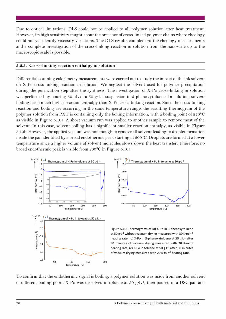
70 5.Polymer cross-linking in bulk material and thin films
Due to optical limitations, DLS could not be applied to all polymer solution after heat treatment.
However, its high sensitivity taught about the presence of cross-linked polymer chains where rheology
could not yet identify viscosity variations. The DLS results complement the rheology measurements
and a complete investigation of the cross-linking reaction in solution from the nanoscale up to the
macroscopic scale is possible.
5.2.3. Cross-linking reaction enthalpy in solution
Differential scanning calorimetry measurements were carried out to study the impact of the ink solvent
on X-Po cross-linking reaction in solution. We neglect the solvent used for polymer precipitation
during the purification step after the synthesis. The investigation of X-Po cross-linking in solution
was performed by pouring 30 µL of a 50 g∙L-1 suspension in 3-phenoxytoluene. In solution, solvent
boiling has a much higher reaction enthalpy than X-Po cross-linking reaction. Since the cross-linking
reaction and boiling are occurring in the same temperature range, the resulting thermogram of the
polymer solution from PXT is containing only the boiling information, with a boiling point of 270°C
as visible in Figure 5.10a. A short vacuum run was applied to another sample to remove most of the
solvent. In this case, solvent boiling has a significant smaller reaction enthalpy, as visible in Figure
5.10b. However, the applied vacuum was not enough to remove all solvent leading to droplet formation
inside the pan identified by a broad endothermic peak starting at 200°C. Droplets are formed at a lower
temperature since a higher volume of solvent molecules slows down the heat transfer. Therefore, no
broad endothermic peak is visible from 200°C in Figure 5.10a.
Figure 5.10: Thermograms of (a) X-Po in 3-phenoxytoluene
at 50 g∙L-1 without vacuum drying measured with 30 K∙min-1
heating rate, (b) X-Po in 3-phenoxytoluene at 50 g∙L-1 after
30 minutes of vacuum drying measured with 20 K∙min-1
heating rate, (c) X-Po in toluene at 50 g∙L-1 after 30 minutes
of vacuum drying measured with 20 K∙min-1 heating rate.
To confirm that the endothermic signal is boiling, a polymer solution was made from another solvent
of different boiling point. X-Po was dissolved in toluene at 50 g∙L-1, then poured in a DSC pan and
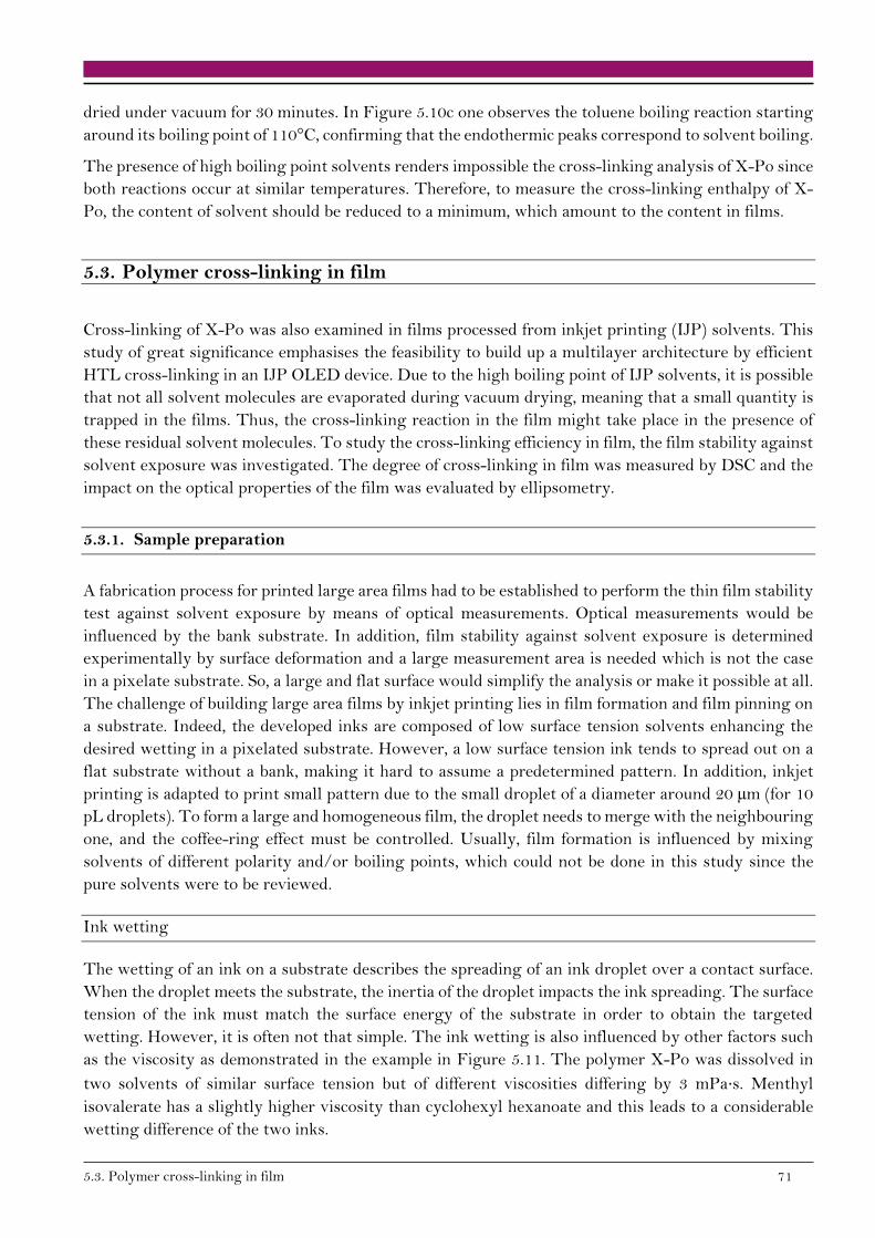
5.3. Polymer cross-linking in film 71
dried under vacuum for 30 minutes. In Figure 5.10c one observes the toluene boiling reaction starting
around its boiling point of 110°C, confirming that the endothermic peaks correspond to solvent boiling.
The presence of high boiling point solvents renders impossible the cross-linking analysis of X-Po since
both reactions occur at similar temperatures. Therefore, to measure the cross-linking enthalpy of X-
Po, the content of solvent should be reduced to a minimum, which amount to the content in films.
5.3. Polymer cross-linking in film
Cross-linking of X-Po was also examined in films processed from inkjet printing (IJP) solvents. This
study of great significance emphasises the feasibility to build up a multilayer architecture by efficient
HTL cross-linking in an IJP OLED device. Due to the high boiling point of IJP solvents, it is possible
that not all solvent molecules are evaporated during vacuum drying, meaning that a small quantity is
trapped in the films. Thus, the cross-linking reaction in the film might take place in the presence of
these residual solvent molecules. To study the cross-linking efficiency in film, the film stability against
solvent exposure was investigated. The degree of cross-linking in film was measured by DSC and the
impact on the optical properties of the film was evaluated by ellipsometry.
5.3.1. Sample preparation
A fabrication process for printed large area films had to be established to perform the thin film stability
test against solvent exposure by means of optical measurements. Optical measurements would be
influenced by the bank substrate. In addition, film stability against solvent exposure is determined
experimentally by surface deformation and a large measurement area is needed which is not the case
in a pixelate substrate. So, a large and flat surface would simplify the analysis or make it possible at all.
The challenge of building large area films by inkjet printing lies in film formation and film pinning on
a substrate. Indeed, the developed inks are composed of low surface tension solvents enhancing the
desired wetting in a pixelated substrate. However, a low surface tension ink tends to spread out on a
flat substrate without a bank, making it hard to assume a predetermined pattern. In addition, inkjet
printing is adapted to print small pattern due to the small droplet of a diameter around 20 µm (for 10
pL droplets). To form a large and homogeneous film, the droplet needs to merge with the neighbouring
one, and the coffee-ring effect must be controlled. Usually, film formation is influenced by mixing
solvents of different polarity and/or boiling points, which could not be done in this study since the
pure solvents were to be reviewed.
Ink wetting
The wetting of an ink on a substrate describes the spreading of an ink droplet over a contact surface.
When the droplet meets the substrate, the inertia of the droplet impacts the ink spreading. The surface
tension of the ink must match the surface energy of the substrate in order to obtain the targeted
wetting. However, it is often not that simple. The ink wetting is also influenced by other factors such
as the viscosity as demonstrated in the example in Figure 5.11. The polymer X-Po was dissolved in
two solvents of similar surface tension but of different viscosities differing by 3 mPa∙s. Menthyl
isovalerate has a slightly higher viscosity than cyclohexyl hexanoate and this leads to a considerable
wetting difference of the two inks.
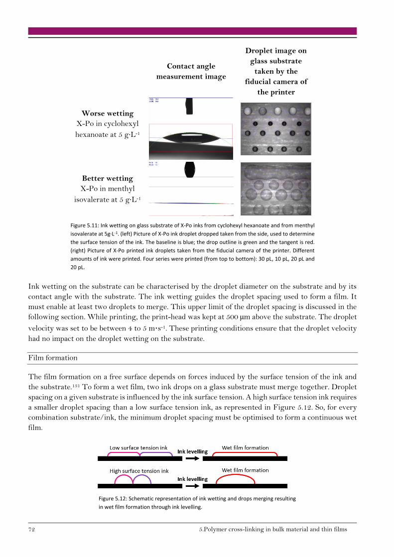
72 5.Polymer cross-linking in bulk material and thin films
Contact angle
measurement image
Droplet image on
glass substrate
taken by the
fiducial camera of
the printer
Worse wetting
X-Po in cyclohexyl
hexanoate at 5 g∙L-1
Better wetting
X-Po in menthyl
isovalerate at 5 g∙L-1
Figure 5.11: Ink wetting on glass substrate of X-Po inks from cyclohexyl hexanoate and from menthyl
isovalerate at 5g·L-1. (left) Picture of X-Po ink droplet dropped taken from the side, used to determine
the surface tension of the ink. The baseline is blue; the drop outline is green and the tangent is red.
(right) Picture of X-Po printed ink droplets taken from the fiducial camera of the printer. Different
amounts of ink were printed. Four series were printed (from top to bottom): 30 pL, 10 pL, 20 pL and
20 pL.
Ink wetting on the substrate can be characterised by the droplet diameter on the substrate and by its
contact angle with the substrate. The ink wetting guides the droplet spacing used to form a film. It
must enable at least two droplets to merge. This upper limit of the droplet spacing is discussed in the
following section. While printing, the print-head was kept at 500 µm above the substrate. The droplet
velocity was set to be between 4 to 5 m∙s-1. These printing conditions ensure that the droplet velocity
had no impact on the droplet wetting on the substrate.
Film formation
The film formation on a free surface depends on forces induced by the surface tension of the ink and
the substrate.131 To form a wet film, two ink drops on a glass substrate must merge together. Droplet
spacing on a given substrate is influenced by the ink surface tension. A high surface tension ink requires
a smaller droplet spacing than a low surface tension ink, as represented in Figure 5.12. So, for every
combination substrate/ink, the minimum droplet spacing must be optimised to form a continuous wet
film.
Figure 5.12: Schematic representation of ink wetting and drops merging resulting
in wet film formation through ink levelling.
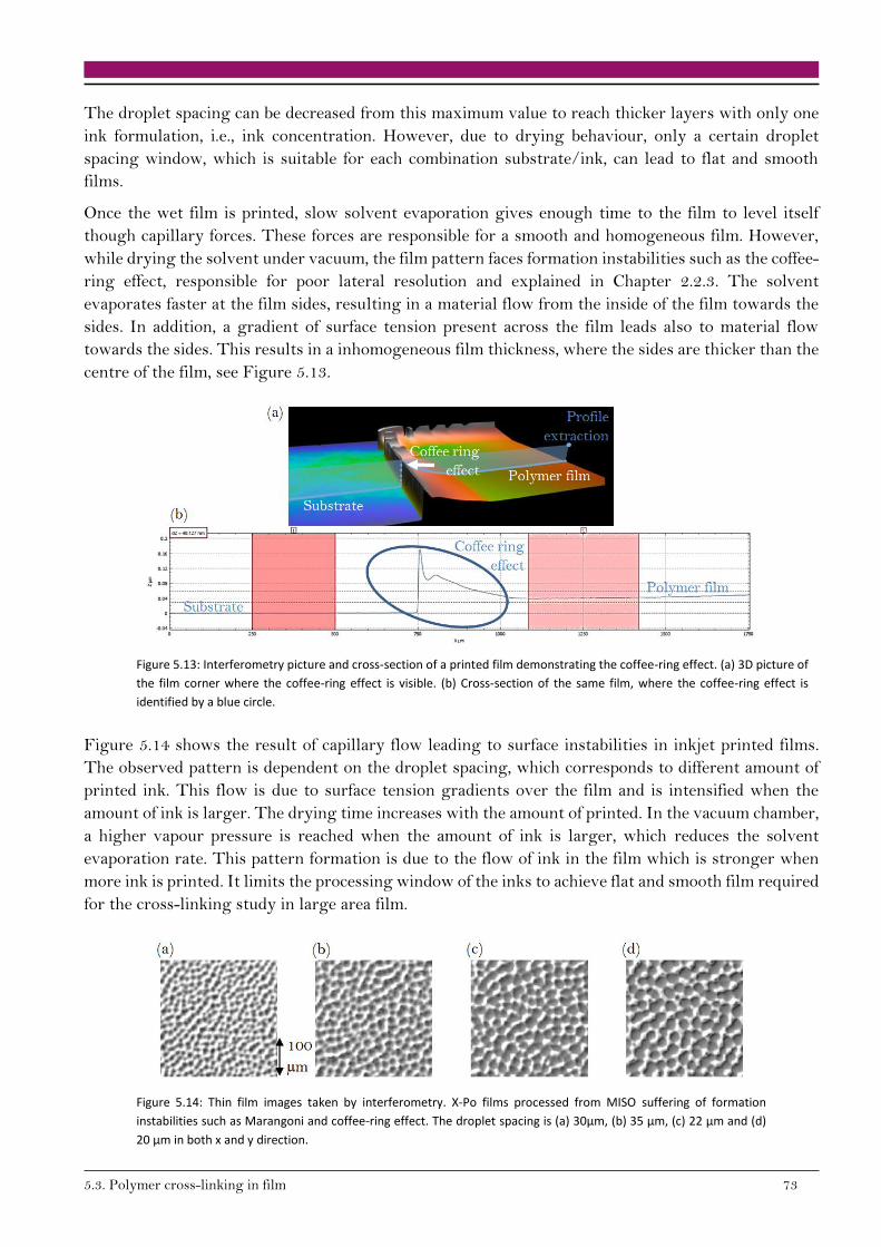
5.3. Polymer cross-linking in film 73
The droplet spacing can be decreased from this maximum value to reach thicker layers with only one
ink formulation, i.e., ink concentration. However, due to drying behaviour, only a certain droplet
spacing window, which is suitable for each combination substrate/ink, can lead to flat and smooth
films.
Once the wet film is printed, slow solvent evaporation gives enough time to the film to level itself
though capillary forces. These forces are responsible for a smooth and homogeneous film. However,
while drying the solvent under vacuum, the film pattern faces formation instabilities such as the coffee-
ring effect, responsible for poor lateral resolution and explained in Chapter 2.2.3. The solvent
evaporates faster at the film sides, resulting in a material flow from the inside of the film towards the
sides. In addition, a gradient of surface tension present across the film leads also to material flow
towards the sides. This results in a inhomogeneous film thickness, where the sides are thicker than the
centre of the film, see Figure 5.13.
Figure 5.13: Interferometry picture and cross-section of a printed film demonstrating the coffee-ring effect. (a) 3D picture of
the film corner where the coffee-ring effect is visible. (b) Cross-section of the same film, where the coffee-ring effect is
identified by a blue circle.
Figure 5.14 shows the result of capillary flow leading to surface instabilities in inkjet printed films.
The observed pattern is dependent on the droplet spacing, which corresponds to different amount of
printed ink. This flow is due to surface tension gradients over the film and is intensified when the
amount of ink is larger. The drying time increases with the amount of printed. In the vacuum chamber,
a higher vapour pressure is reached when the amount of ink is larger, which reduces the solvent
evaporation rate. This pattern formation is due to the flow of ink in the film which is stronger when
more ink is printed. It limits the processing window of the inks to achieve flat and smooth film required
for the cross-linking study in large area film.
Figure 5.14: Thin film images taken by interferometry. X-Po films processed from MISO suffering of formation
instabilities such as Marangoni and coffee-ring effect. The droplet spacing is (a) 30µm, (b) 35 µm, (c) 22 µm and (d)
20 µm in both x and y direction.
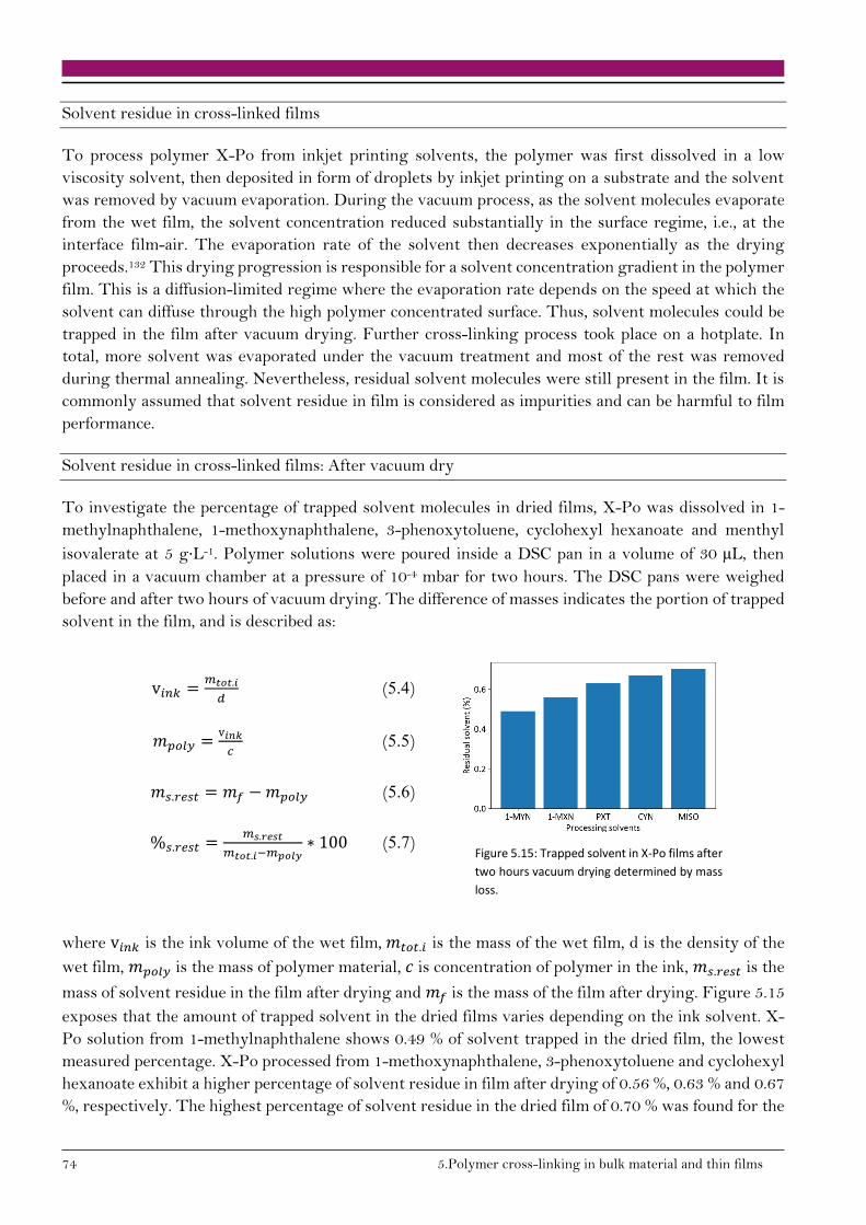
74 5.Polymer cross-linking in bulk material and thin films
Solvent residue in cross-linked films
To process polymer X-Po from inkjet printing solvents, the polymer was first dissolved in a low
viscosity solvent, then deposited in form of droplets by inkjet printing on a substrate and the solvent
was removed by vacuum evaporation. During the vacuum process, as the solvent molecules evaporate
from the wet film, the solvent concentration reduced substantially in the surface regime, i.e., at the
interface film-air. The evaporation rate of the solvent then decreases exponentially as the drying
proceeds.132 This drying progression is responsible for a solvent concentration gradient in the polymer
film. This is a diffusion-limited regime where the evaporation rate depends on the speed at which the
solvent can diffuse through the high polymer concentrated surface. Thus, solvent molecules could be
trapped in the film after vacuum drying. Further cross-linking process took place on a hotplate. In
total, more solvent was evaporated under the vacuum treatment and most of the rest was removed
during thermal annealing. Nevertheless, residual solvent molecules were still present in the film. It is
commonly assumed that solvent residue in film is considered as impurities and can be harmful to film
performance.
Solvent residue in cross-linked films: After vacuum dry
To investigate the percentage of trapped solvent molecules in dried films, X-Po was dissolved in 1-
methylnaphthalene, 1-methoxynaphthalene, 3-phenoxytoluene, cyclohexyl hexanoate and menthyl
isovalerate at 5 g∙L-1. Polymer solutions were poured inside a DSC pan in a volume of 30 µL, then
placed in a vacuum chamber at a pressure of 10-4 mbar for two hours. The DSC pans were weighed
before and after two hours of vacuum drying. The difference of masses indicates the portion of trapped
solvent in the film, and is described as:
where v𝑖𝑛𝑘 is the ink volume of the wet film, 𝑚𝑡𝑜𝑡.𝑖 is the mass of the wet film, d is the density of the
wet film, 𝑚𝑝𝑜𝑙𝑦 is the mass of polymer material, 𝑐 is concentration of polymer in the ink, 𝑚𝑠.𝑟𝑒𝑠𝑡 is the
mass of solvent residue in the film after drying and 𝑚𝑓 is the mass of the film after drying. Figure 5.15
exposes that the amount of trapped solvent in the dried films varies depending on the ink solvent. X-
Po solution from 1-methylnaphthalene shows 0.49 % of solvent trapped in the dried film, the lowest
measured percentage. X-Po processed from 1-methoxynaphthalene, 3-phenoxytoluene and cyclohexyl
hexanoate exhibit a higher percentage of solvent residue in film after drying of 0.56 %, 0.63 % and 0.67
%, respectively. The highest percentage of solvent residue in the dried film of 0.70 % was found for the
v𝑖𝑛𝑘 =𝑚𝑡𝑜𝑡.𝑖
𝑑 (5.4)
𝑚𝑝𝑜𝑙𝑦 =v𝑖𝑛𝑘
𝑐 (5.5)
𝑚𝑠.𝑟𝑒𝑠𝑡 = 𝑚𝑓 − 𝑚𝑝𝑜𝑙𝑦 (5.6)
%𝑠.𝑟𝑒𝑠𝑡 =𝑚𝑠.𝑟𝑒𝑠𝑡
𝑚𝑡𝑜𝑡.𝑖−𝑚𝑝𝑜𝑙𝑦∗ 100 (5.7)
Figure 5.15: Trapped solvent in X-Po films after
two hours vacuum drying determined by mass
loss.
5.3. Polymer cross-linking in film 75
X-Po solution from menthyl isovalerate. So it can be concluded that solvent evaporation from a wet
polymer film depends on the ink solvent and is directly correlated to the polymer-solvent affinity.133-
134 A poor polymer-solvent interaction such as X-Po and menthyl isovalerate favours a fast evaporation
rate which leads to a high polymer density at the open surface and therefore traps more solvent in the
bulk of the film. On the contrary, X-Po film from 1-methylnaphthalene, solvent exhibiting a good
affinity to X-Po, tends to have a slower evaporation rate, thus the evaporation is constant over time
due to the absence of a polymer density gradient in the drying surface of the wet film.
Solvent residue in cross-linked films: After annealing
In the actual process of fabricating an X-Po layer of an OLED, an annealing step followed the vacuum
drying which is a second opportunity for the solvent to evaporate. A new method has been developed
to investigate solvent residue in large area printed films after annealing with the objective to identify
whether trapped solvent molecules remain in the film even after the annealing step. In this
measurement, X-Po was processed from 3-phenoxytoluene on a glass substrate. The measurement
procedure consists of placing the substrate inside a sample holder, with the face pointing down so that
the X-Po film was directed toward the bottom (see Figure 5.16). 200 µL of toluene, a solvent miscible
with the test solvent 3-phenoxytoluene, was poured into the sample holder which was then sealed to
avoid solvent evaporation. After ten minutes, the solution was filled into a gas chromatographic vial
to measure the amount of 3-phenoxytoluene found in the toluene solution (see procedure represented
in Figure 5.16).
Figure 5.16: Newly developed measurement procedure to determine the solvent residue in X-Po film after the annealing step.
The amount of solvent residue is defined as the ratio of the residual solvent weight divided by the
printed ink weight. Even though the GC method is very sensitive and permits the determination of
nanograms, resulting in parts per million (ppm) solvent residue, the sample preparation reproducibility
was not sufficient to rationalise deeper investigation. The only reasonable result was obtained from a
printed film of X-Po from 3-phenoxytoluene being cross-linking at 225°C for 30 minutes. It led to a
solvent residue in film between 5 ppm to 20 ppm in weight. For all the other solvents it is assumed
that printed X-Po polymer films exhibit similar solvent concentrations of about 20 ppm in weight
where the difference between solvents is smaller than the uncertainty in the sample preparation.
It can be concluded that after annealing and before subsequent printing, the five printed films are in
similar conditions regarding solvent residue. There was no indication that solvent residue explains for
any layer discrepancy in the performance of films processed from the tested solvents.
5.3.2. Stability of thin films against solvent exposure
One main challenge when studying the intermixing of subsequent solution-processed layers is the
hidden nature of the resulting interface. Usually the stability of thin films against a subsequent solvent
is tested by a rinsing test of spin coated films. By this procedure, the stability is characterised by the
PXT solvent
weight residual
in X-Po layer
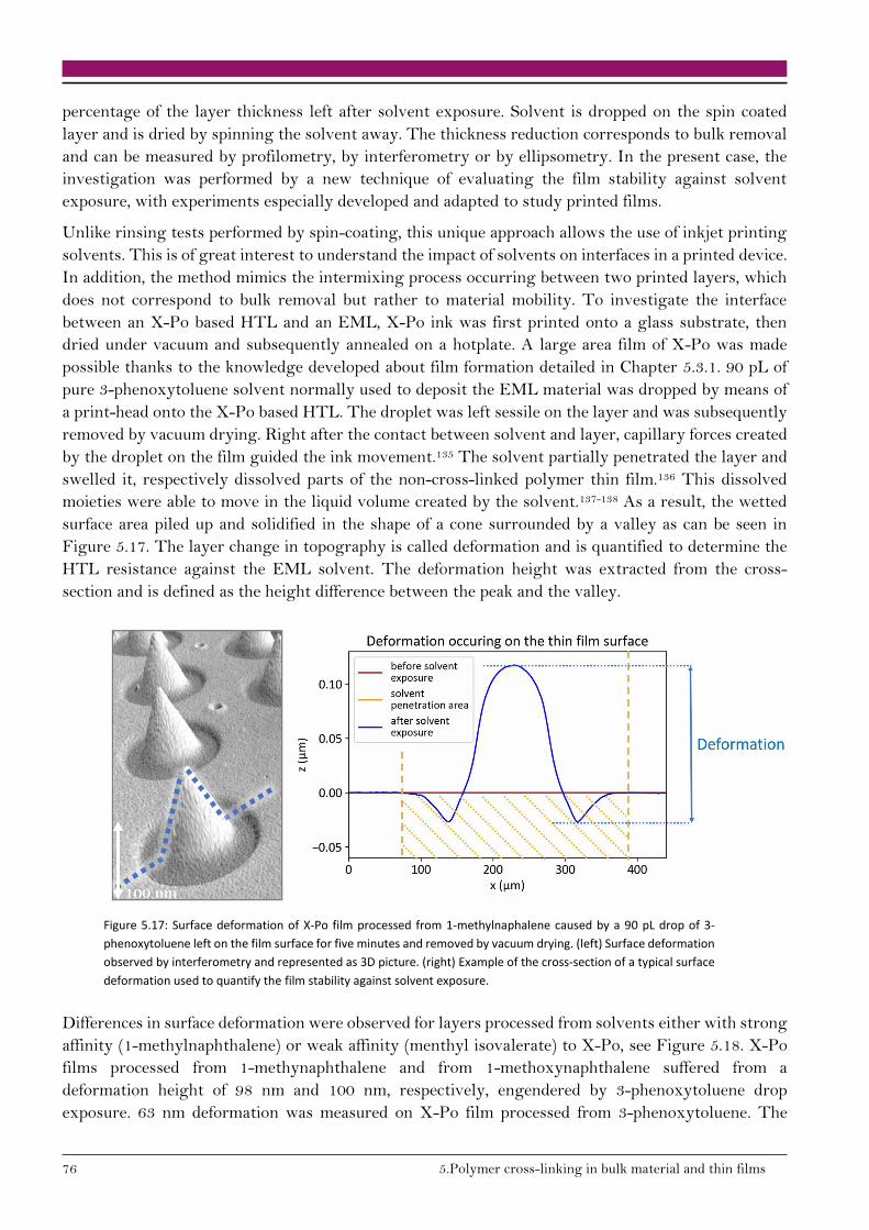
76 5.Polymer cross-linking in bulk material and thin films
percentage of the layer thickness left after solvent exposure. Solvent is dropped on the spin coated
layer and is dried by spinning the solvent away. The thickness reduction corresponds to bulk removal
and can be measured by profilometry, by interferometry or by ellipsometry. In the present case, the
investigation was performed by a new technique of evaluating the film stability against solvent
exposure, with experiments especially developed and adapted to study printed films.
Unlike rinsing tests performed by spin-coating, this unique approach allows the use of inkjet printing
solvents. This is of great interest to understand the impact of solvents on interfaces in a printed device.
In addition, the method mimics the intermixing process occurring between two printed layers, which
does not correspond to bulk removal but rather to material mobility. To investigate the interface
between an X-Po based HTL and an EML, X-Po ink was first printed onto a glass substrate, then
dried under vacuum and subsequently annealed on a hotplate. A large area film of X-Po was made
possible thanks to the knowledge developed about film formation detailed in Chapter 5.3.1. 90 pL of
pure 3-phenoxytoluene solvent normally used to deposit the EML material was dropped by means of
a print-head onto the X-Po based HTL. The droplet was left sessile on the layer and was subsequently
removed by vacuum drying. Right after the contact between solvent and layer, capillary forces created
by the droplet on the film guided the ink movement.135 The solvent partially penetrated the layer and
swelled it, respectively dissolved parts of the non-cross-linked polymer thin film.136 This dissolved
moieties were able to move in the liquid volume created by the solvent.137-138 As a result, the wetted
surface area piled up and solidified in the shape of a cone surrounded by a valley as can be seen in
Figure 5.17. The layer change in topography is called deformation and is quantified to determine the
HTL resistance against the EML solvent. The deformation height was extracted from the cross-
section and is defined as the height difference between the peak and the valley.
Figure 5.17: Surface deformation of X-Po film processed from 1-methylnaphalene caused by a 90 pL drop of 3-
phenoxytoluene left on the film surface for five minutes and removed by vacuum drying. (left) Surface deformation
observed by interferometry and represented as 3D picture. (right) Example of the cross-section of a typical surface
deformation used to quantify the film stability against solvent exposure.
Differences in surface deformation were observed for layers processed from solvents either with strong
affinity (1-methylnaphthalene) or weak affinity (menthyl isovalerate) to X-Po, see Figure 5.18. X-Po
films processed from 1-methynaphthalene and from 1-methoxynaphthalene suffered from a
deformation height of 98 nm and 100 nm, respectively, engendered by 3-phenoxytoluene drop
exposure. 63 nm deformation was measured on X-Po film processed from 3-phenoxytoluene. The
100 nm
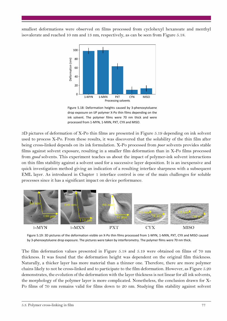
5.3. Polymer cross-linking in film 77
smallest deformations were observed on films processed from cyclohexyl hexanoate and menthyl
isovalerate and reached 10 nm and 13 nm, respectively, as can be seen from Figure 5.18.
Figure 5.18: Deformation heights caused by 3-phenoxytoluene
drop exposure on IJP polymer X-Po thin films depending on the
ink solvent. The polymer films were 70 nm thick and were
processed from 1-MYN, 1-MXN, PXT, CYX and MISO.
3D pictures of deformation of X-Po thin films are presented in Figure 5.19 depending on ink solvent
used to process X-Po. From these results, it was discovered that the solubility of the thin film after
being cross-linked depends on its ink formulation. X-Po processed from poor solvents provides stable
films against solvent exposure, resulting in a smaller film deformation than in X-Po films processed
from good solvents. This experiment teaches us about the impact of polymer-ink solvent interactions
on thin film stability against a solvent used for a successive layer deposition. It is an inexpensive and
quick investigation method giving an indication of a resulting interface sharpness with a subsequent
EML layer. As introduced in Chapter 1 interface control is one of the main challenges for soluble
processes since it has a significant impact on device performance.
Figure 5.19: 3D pictures of the deformation visible on X-Po thin films processed from 1-MYN, 1-MXN, PXT, CYX and MISO caused
by 3-phenoxytoluene drop exposure. The pictures were taken by interferometry. The polymer films were 70 nm thick.
The film deformation values presented in Figure 5.18 and 5.19 were obtained on films of 70 nm
thickness. It was found that the deformation height was dependent on the original film thickness.
Naturally, a thicker layer has more material than a thinner one. Therefore, there are more polymer
chains likely to not be cross-linked and to participate to the film deformation. However, as Figure 5.20
demonstrates, the evolution of the deformation with the layer thickness is not linear for all ink solvents,
the morphology of the polymer layer is more complicated. Nonetheless, the conclusion drawn for X-
Po films of 70 nm remains valid for films down to 20 nm. Studying film stability against solvent
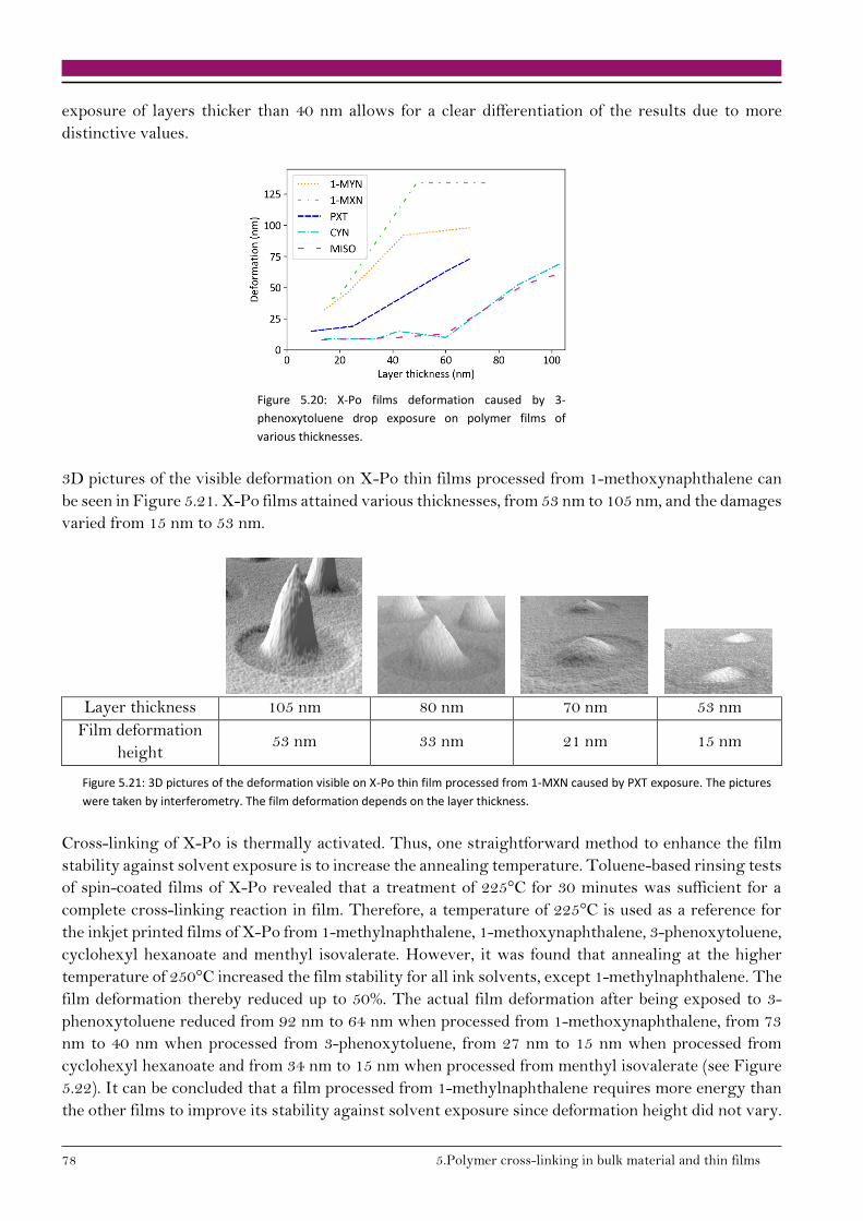
78 5.Polymer cross-linking in bulk material and thin films
exposure of layers thicker than 40 nm allows for a clear differentiation of the results due to more
distinctive values.
Figure 5.20: X-Po films deformation caused by 3-
phenoxytoluene drop exposure on polymer films of
various thicknesses.
3D pictures of the visible deformation on X-Po thin films processed from 1-methoxynaphthalene can
be seen in Figure 5.21. X-Po films attained various thicknesses, from 53 nm to 105 nm, and the damages
varied from 15 nm to 53 nm.
Layer thickness 105 nm 80 nm 70 nm 53 nm
Film deformation
height 53 nm 33 nm 21 nm 15 nm
Figure 5.21: 3D pictures of the deformation visible on X-Po thin film processed from 1-MXN caused by PXT exposure. The pictures
were taken by interferometry. The film deformation depends on the layer thickness.
Cross-linking of X-Po is thermally activated. Thus, one straightforward method to enhance the film
stability against solvent exposure is to increase the annealing temperature. Toluene-based rinsing tests
of spin-coated films of X-Po revealed that a treatment of 225°C for 30 minutes was sufficient for a
complete cross-linking reaction in film. Therefore, a temperature of 225°C is used as a reference for
the inkjet printed films of X-Po from 1-methylnaphthalene, 1-methoxynaphthalene, 3-phenoxytoluene,
cyclohexyl hexanoate and menthyl isovalerate. However, it was found that annealing at the higher
temperature of 250°C increased the film stability for all ink solvents, except 1-methylnaphthalene. The
film deformation thereby reduced up to 50%. The actual film deformation after being exposed to 3-
phenoxytoluene reduced from 92 nm to 64 nm when processed from 1-methoxynaphthalene, from 73
nm to 40 nm when processed from 3-phenoxytoluene, from 27 nm to 15 nm when processed from
cyclohexyl hexanoate and from 34 nm to 15 nm when processed from menthyl isovalerate (see Figure
5.22). It can be concluded that a film processed from 1-methylnaphthalene requires more energy than
the other films to improve its stability against solvent exposure since deformation height did not vary.

5.3. Polymer cross-linking in film 79
For example, a longer annealing duration should lead to a reduced film deformation after solvent
exposure. 1-methylnaphthalene is the solvent exhibiting the strongest interaction with X-Po resulting
in a poorly stable film against solvent exposure.
Figure 5.22: Film deformation following exposure to 3-
phenoxytoluene on the 70 nm thick polymer films after
annealing at different temperatures.
3D pictures of deformation of X-Po thin films depending on ink solvent and annealing temperature are
displayed in Figure 5.23.
HTL
annealing
temperature
HTL processed from
1-MYN 1-MYN PXT CYX MISO
225°C
250°C
Figure 5.23: 3D pictures of the deformation visible on X-Po thin films processed from 1-MYN, 1-MXN, PXT, CYX and
MISO and annealed at 225°C and 250°C, respectively, caused by PXT exposure. The pictures were taken by
interferometry. The polymer films are 70 nm thick.
By these experiments, the difference of printed thin films depending on the ink solvent can be
investigated and quantified. A direct correlation between ink solvent and thin film stability against
solvent exposure was identified. Polymer films processed from poor solvents exhibit a smaller
deformation after solvent exposure than polymer films of same thickness processed from good solvents
for otherwise identical processes, i.e. the annealing temperature and duration. Thicker layers display a
higher deformation than thinner layers of the same material and ink solvent. The film deformation can
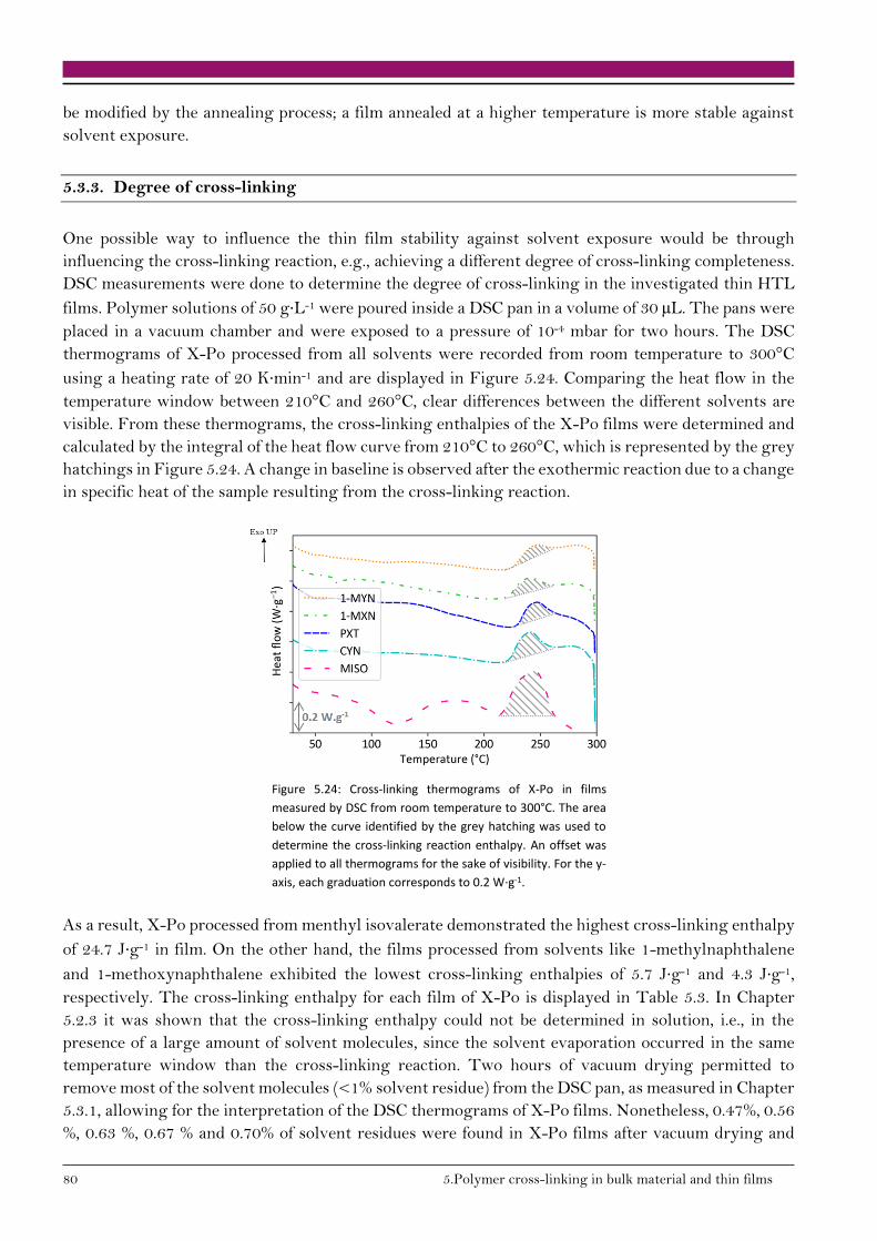
80 5.Polymer cross-linking in bulk material and thin films
be modified by the annealing process; a film annealed at a higher temperature is more stable against
solvent exposure.
5.3.3. Degree of cross-linking
One possible way to influence the thin film stability against solvent exposure would be through
influencing the cross-linking reaction, e.g., achieving a different degree of cross-linking completeness.
DSC measurements were done to determine the degree of cross-linking in the investigated thin HTL
films. Polymer solutions of 50 g∙L-1 were poured inside a DSC pan in a volume of 30 µL. The pans were
placed in a vacuum chamber and were exposed to a pressure of 10-4 mbar for two hours. The DSC
thermograms of X-Po processed from all solvents were recorded from room temperature to 300°C
using a heating rate of 20 K∙min-1 and are displayed in Figure 5.24. Comparing the heat flow in the
temperature window between 210°C and 260°C, clear differences between the different solvents are
visible. From these thermograms, the cross-linking enthalpies of the X-Po films were determined and
calculated by the integral of the heat flow curve from 210°C to 260°C, which is represented by the grey
hatchings in Figure 5.24. A change in baseline is observed after the exothermic reaction due to a change
in specific heat of the sample resulting from the cross-linking reaction.
Figure 5.24: Cross-linking thermograms of X-Po in films
measured by DSC from room temperature to 300°C. The area
below the curve identified by the grey hatching was used to
determine the cross-linking reaction enthalpy. An offset was
applied to all thermograms for the sake of visibility. For the y-
axis, each graduation corresponds to 0.2 W∙g-1.
As a result, X-Po processed from menthyl isovalerate demonstrated the highest cross-linking enthalpy
of 24.7 J∙g-1 in film. On the other hand, the films processed from solvents like 1-methylnaphthalene
and 1-methoxynaphthalene exhibited the lowest cross-linking enthalpies of 5.7 J∙g-1 and 4.3 J∙g-1,
respectively. The cross-linking enthalpy for each film of X-Po is displayed in Table 5.3. In Chapter
5.2.3 it was shown that the cross-linking enthalpy could not be determined in solution, i.e., in the
presence of a large amount of solvent molecules, since the solvent evaporation occurred in the same
temperature window than the cross-linking reaction. Two hours of vacuum drying permitted to
remove most of the solvent molecules (<1% solvent residue) from the DSC pan, as measured in Chapter
5.3.1, allowing for the interpretation of the DSC thermograms of X-Po films. Nonetheless, 0.47%, 0.56
%, 0.63 %, 0.67 % and 0.70% of solvent residues were found in X-Po films after vacuum drying and

5.3. Polymer cross-linking in film 81
processed from 1-methylnaphthalene, 1-methoxynaphthalene, 3-phenoxytoluene, cyclohexyl
hexanoate and menthyl isovalerate, respectively. Films processed from menthyl isovalerate display the
highest cross-linking enthalpy even though it is the film retaining the highest percentage of solvent
after vacuum drying. So, it can be assumed that even higher cross-linking enthalpies could be reached
in X-Po films processed from menthyl isovalerate if the drying process would be further optimised to
retain the minimum amount of solvent possible. Trapped solvent in film is of importance for DSC
measurements since the cross-linking enthalpy is determined by a single heat ramp from room
temperature to 300°C at 20 K·min-1. In a printed film, cross-linking occurs during 30 minutes at a
constant temperature of 225°C. It was shown in Chapter 5.3.1 that after this annealing process the
residual solvent concentration is similar, independent of the ink solvent. Thus, trapped solvent cannot
explain the discrepancy of the cross-linking degree in printed films.
Thereby the degree of cross-linking of X-Po in films 𝑋(𝑆𝑥) is established by the ratio between cross-
linking enthalpy of the polymer in film (∆𝐻(𝑆𝑥)) and cross-linking enthalpy in powder without solvent
(∆𝐻(𝑆0)). Thereby the cross-linking enthalpy ∆𝐻(𝑆𝑥) is directly correlated to the cross-linking reaction
density.139 According to Lu and al.140 it yields:
𝑋(𝑆𝑥) =
∆𝐻(𝑆𝑥)
∆𝐻(𝑆0)
(5.8)
Table 5.3: Comparison of cross-linking enthalpies and peaks of reaction of X-Po polymer powder and of X-Po films
obtained from the five IJP solvent solutions after two hours vacuum drying, measured by DSC from room
temperature to 300°C. The X-Po powder is used without solvent.
Film ink solvent Cross-linking
enthalpy [J∙g-1]
Peak of
reaction [°C]
Normalised degree
of cross-linking
1-MYN 5.7 241 0.12
1-MXN 4.3 248 0.09
PXT 6.4 246 0.14
CYX 9.4 241 0.20
MISO 24.7 246 0.53
X-Po powder without
solvent 46.7 240 1
The impact of ink solvent on the degree of cross-linking of polymer X-Po is in accordance with what
was observed in solution and assessed by ink viscosity measurement, see Chapter 5.2.1. The polymer
solution prepared using poor solvents cross-link at lower temperature than polymer solutions prepared
using good solvents. This result is paramount since it explains what happens in the X-Po film bulk
when it is processed from various solvents. It brings a further understanding of the film stability
experiment against solvent exposure. When processed from a poor solvent, X-Po reaches a higher
cross-linking degree in film than a film processed from a good solvent. The high cross-linking degree
awards an enhanced stability against solvent exposure to the film as demonstrated in Chapter 5.3.2.

82 5.Polymer cross-linking in bulk material and thin films
5.3.4. Variation of optical properties
Optical properties of thin films can be related to their physical characteristics, since optical properties
carry information about film thickness, composition and density.141 Ellipsometry is a very sensitive
and non-destructing measurement technique for optical properties of thin films. Using the
spectroscopic ellipsometry over a broad range of wavelengths from ultraviolet to infrared increases the
measurement options and more complex systems can be characterised.
In order to study the impact of the cross-linking degree on the polymer thin film optical properties, X-
Po was processed from 1-methylnaphthalene, 3-phenoxytoluene and menthyl isovalerate on a quartz
substrate to achieve a large area film (4 cm²) of 70 nm thickness. These three ink solvents were chosen
since X-Po showed the lowest/highest cross-linking degree in films processed from 1-
methylnaphthalene/menthyl isovalerate, and a median value in films processed from 3-
phenoxytoluene. After vacuum drying, the thin films were annealed at 160°C, 200°C and 225°C for 30
minutes on a hotplate to vary the cross-linking degree for a given ink solvent. After measuring thin
film absorption in reflection and in transmission, the measured data were fitted with a special physical
model of the fully cross-linked X-Po polymer. In this study, the spectra of inkjet printed films of X-Po
were compared to the corresponding optical properties of a cross-linked X-Po spin-coated film,
constituting the n and k constants. The spin-coated film was described as a one film with one refractive
index n and one extinction coefficient k. The optical constants of X-Po cross-linked spin-coated films
were known, and a model for X-Po was built from these films. The model was calculated from three
X-Po spin-coated films after cross-linking at 225°C for 30 minutes. If the ink solvent does not have an
impact on the optical properties of the printed film, all printed films should be describable by the model
for the spin-coated films. To test this hypothesis, the existing model was used to fit each measurement
of printed films, and the MSE was determined. The higher the MSE, the less meaningful is the model
to describe the printed layer.
The calculated MSEs are reported in Figure 5.25. Considering that the films were transparent and
non-rough, low MSE should be targeted. A maximum MSE value of 5 is considered to be a good value
in this analysis knowing that the calculation runs over a wide range of wavelengths. When the thin
films were annealed at 225°C, the MSE of X-Po thin films processed from 1-methylnaphthalene, 3-
phenoxytoluene and menthyl isovalerate are approximately equal to MSE = 5. It can be concluded that
after a heating treatment of 225°C, X-Po films processed from 1-methylnaphthalene, 3-
phenoxytoluene and menthyl isovalerate exhibits a similar optical performance as a cross-linked spin-
coated film.
Figure 5.25: Mean square error
calculated for X-Po thin films’
absorption over wavelength range from
250 to 1000 nm. The thin films were
processed from 1-MYN, PXT and MISO
and were annealed either at 160°C,
200°C or 225°C.
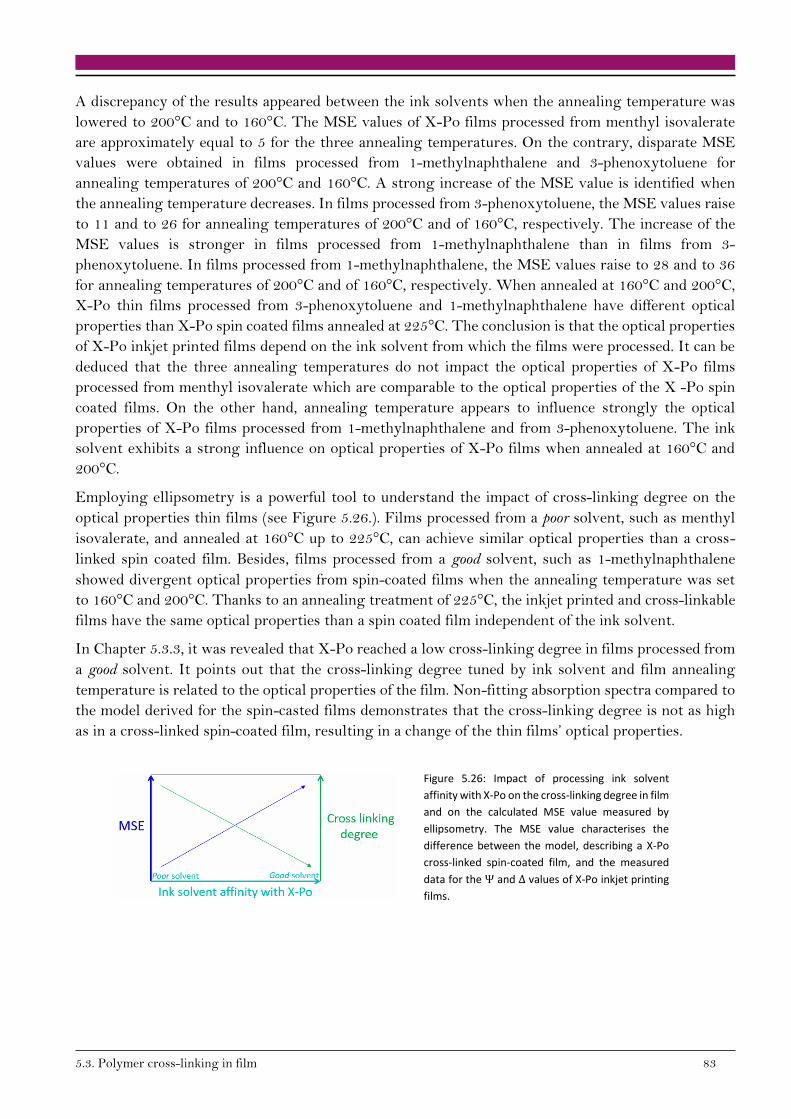
5.3. Polymer cross-linking in film 83
A discrepancy of the results appeared between the ink solvents when the annealing temperature was
lowered to 200°C and to 160°C. The MSE values of X-Po films processed from menthyl isovalerate
are approximately equal to 5 for the three annealing temperatures. On the contrary, disparate MSE
values were obtained in films processed from 1-methylnaphthalene and 3-phenoxytoluene for
annealing temperatures of 200°C and 160°C. A strong increase of the MSE value is identified when
the annealing temperature decreases. In films processed from 3-phenoxytoluene, the MSE values raise
to 11 and to 26 for annealing temperatures of 200°C and of 160°C, respectively. The increase of the
MSE values is stronger in films processed from 1-methylnaphthalene than in films from 3-
phenoxytoluene. In films processed from 1-methylnaphthalene, the MSE values raise to 28 and to 36
for annealing temperatures of 200°C and of 160°C, respectively. When annealed at 160°C and 200°C,
X-Po thin films processed from 3-phenoxytoluene and 1-methylnaphthalene have different optical
properties than X-Po spin coated films annealed at 225°C. The conclusion is that the optical properties
of X-Po inkjet printed films depend on the ink solvent from which the films were processed. It can be
deduced that the three annealing temperatures do not impact the optical properties of X-Po films
processed from menthyl isovalerate which are comparable to the optical properties of the X -Po spin
coated films. On the other hand, annealing temperature appears to influence strongly the optical
properties of X-Po films processed from 1-methylnaphthalene and from 3-phenoxytoluene. The ink
solvent exhibits a strong influence on optical properties of X-Po films when annealed at 160°C and
200°C.
Employing ellipsometry is a powerful tool to understand the impact of cross-linking degree on the
optical properties thin films (see Figure 5.26.). Films processed from a poor solvent, such as menthyl
isovalerate, and annealed at 160°C up to 225°C, can achieve similar optical properties than a cross-
linked spin coated film. Besides, films processed from a good solvent, such as 1-methylnaphthalene
showed divergent optical properties from spin-coated films when the annealing temperature was set
to 160°C and 200°C. Thanks to an annealing treatment of 225°C, the inkjet printed and cross-linkable
films have the same optical properties than a spin coated film independent of the ink solvent.
In Chapter 5.3.3, it was revealed that X-Po reached a low cross-linking degree in films processed from
a good solvent. It points out that the cross-linking degree tuned by ink solvent and film annealing
temperature is related to the optical properties of the film. Non-fitting absorption spectra compared to
the model derived for the spin-casted films demonstrates that the cross-linking degree is not as high
as in a cross-linked spin-coated film, resulting in a change of the thin films’ optical properties.
Figure 5.26: Impact of processing ink solvent
affinity with X-Po on the cross-linking degree in film
and on the calculated MSE value measured by
ellipsometry. The MSE value characterises the
difference between the model, describing a X-Po
cross-linked spin-coated film, and the measured
data for the Ψ and Δ values of X-Po inkjet printing
films.
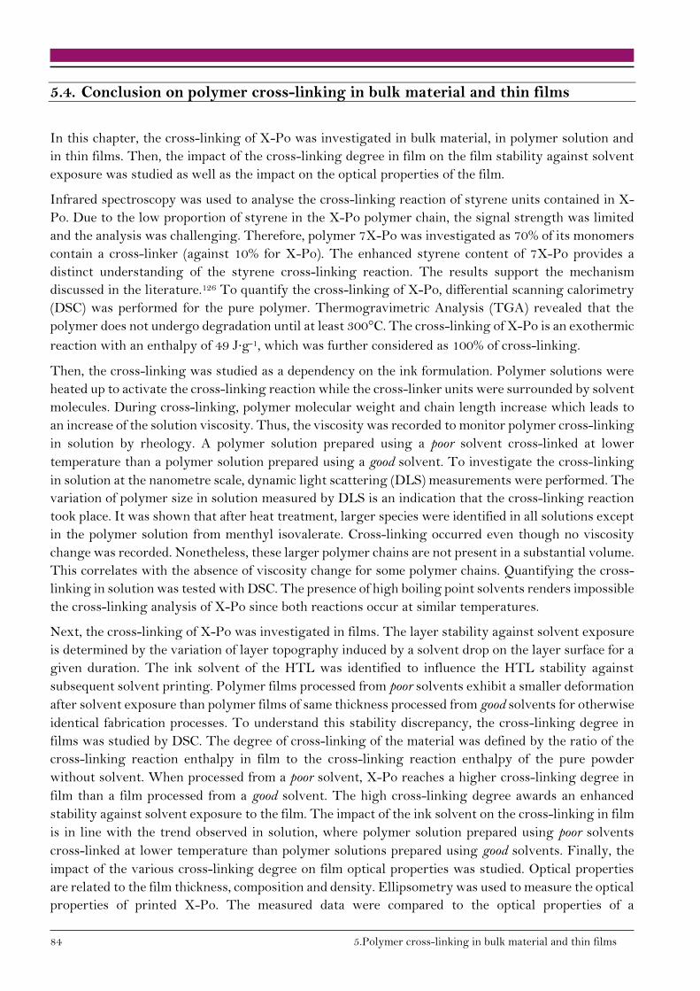
84 5.Polymer cross-linking in bulk material and thin films
5.4. Conclusion on polymer cross-linking in bulk material and thin films
In this chapter, the cross-linking of X-Po was investigated in bulk material, in polymer solution and
in thin films. Then, the impact of the cross-linking degree in film on the film stability against solvent
exposure was studied as well as the impact on the optical properties of the film.
Infrared spectroscopy was used to analyse the cross-linking reaction of styrene units contained in X-
Po. Due to the low proportion of styrene in the X-Po polymer chain, the signal strength was limited
and the analysis was challenging. Therefore, polymer 7X-Po was investigated as 70% of its monomers
contain a cross-linker (against 10% for X-Po). The enhanced styrene content of 7X-Po provides a
distinct understanding of the styrene cross-linking reaction. The results support the mechanism
discussed in the literature.126 To quantify the cross-linking of X-Po, differential scanning calorimetry
(DSC) was performed for the pure polymer. Thermogravimetric Analysis (TGA) revealed that the
polymer does not undergo degradation until at least 300°C. The cross-linking of X-Po is an exothermic
reaction with an enthalpy of 49 J∙g-1, which was further considered as 100% of cross-linking.
Then, the cross-linking was studied as a dependency on the ink formulation. Polymer solutions were
heated up to activate the cross-linking reaction while the cross-linker units were surrounded by solvent
molecules. During cross-linking, polymer molecular weight and chain length increase which leads to
an increase of the solution viscosity. Thus, the viscosity was recorded to monitor polymer cross-linking
in solution by rheology. A polymer solution prepared using a poor solvent cross-linked at lower
temperature than a polymer solution prepared using a good solvent. To investigate the cross-linking
in solution at the nanometre scale, dynamic light scattering (DLS) measurements were performed. The
variation of polymer size in solution measured by DLS is an indication that the cross-linking reaction
took place. It was shown that after heat treatment, larger species were identified in all solutions except
in the polymer solution from menthyl isovalerate. Cross-linking occurred even though no viscosity
change was recorded. Nonetheless, these larger polymer chains are not present in a substantial volume.
This correlates with the absence of viscosity change for some polymer chains. Quantifying the cross-
linking in solution was tested with DSC. The presence of high boiling point solvents renders impossible
the cross-linking analysis of X-Po since both reactions occur at similar temperatures.
Next, the cross-linking of X-Po was investigated in films. The layer stability against solvent exposure
is determined by the variation of layer topography induced by a solvent drop on the layer surface for a
given duration. The ink solvent of the HTL was identified to influence the HTL stability against
subsequent solvent printing. Polymer films processed from poor solvents exhibit a smaller deformation
after solvent exposure than polymer films of same thickness processed from good solvents for otherwise
identical fabrication processes. To understand this stability discrepancy, the cross-linking degree in
films was studied by DSC. The degree of cross-linking of the material was defined by the ratio of the
cross-linking reaction enthalpy in film to the cross-linking reaction enthalpy of the pure powder
without solvent. When processed from a poor solvent, X-Po reaches a higher cross-linking degree in
film than a film processed from a good solvent. The high cross-linking degree awards an enhanced
stability against solvent exposure to the film. The impact of the ink solvent on the cross-linking in film
is in line with the trend observed in solution, where polymer solution prepared using poor solvents
cross-linked at lower temperature than polymer solutions prepared using good solvents. Finally, the
impact of the various cross-linking degree on film optical properties was studied. Optical properties
are related to the film thickness, composition and density. Ellipsometry was used to measure the optical
properties of printed X-Po. The measured data were compared to the optical properties of a

5.4. Conclusion on polymer cross-linking in bulk material and thin films 85
standardised spin-coated X-Po film, which was fully cross-linked. Films processed from a poor solvent
achieved similar optical properties than a cross-linked spin coated film in the whole range of annealing
temperatures. Films processed from a good solvent showed divergent optical properties from spin-
coated films when the annealing temperature was lower than the reference temperature of 225°C.
In this chapter it was shown that a polymer solution made from a poor solvent cross-links at lower
temperature than a polymer solution made from a good solvent. In films, high cross-linking degree was
reached when the polymer X-Po was processed from a poor solvent and led to an enhance film stability
against subsequent solvent printing.142

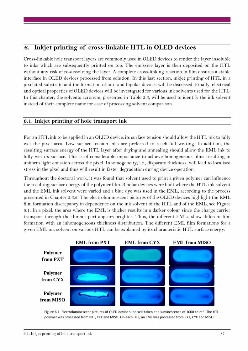
6.1. Inkjet printing of hole transport ink 87
6. Inkjet printing of cross-linkable HTL in OLED devices
Cross-linkable hole transport layers are commonly used in OLED devices to render the layer insoluble
to inks which are subsequently printed on top. The emissive layer is then deposited on the HTL
without any risk of re-dissolving the layer. A complete cross-linking reaction in film ensures a stable
interface in OLED devices processed from solution. In this last section, inkjet printing of HTL in a
pixelated substrate and the formation of uni- and bipolar devices will be discussed. Finally, electrical
and optical properties of OLED devices will be investigated for various ink solvents used for the HTL.
In this chapter, the solvents acronym, presented in Table 3.3, will be used to identify the ink solvent
instead of their complete name for ease of processing solvent comparison.
6.1. Inkjet printing of hole transport ink
For an HTL ink to be applied in an OLED device, its surface tension should allow the HTL ink to fully
wet the pixel area. Low surface tension inks are preferred to reach full wetting. In addition, the
resulting surface energy of the HTL layer after drying and annealing should allow the EML ink to
fully wet its surface. This is of considerable importance to achieve homogeneous films resulting in
uniform light emission across the pixel. Inhomogeneity, i.e., disparate thickness, will lead to localised
stress in the pixel and thus will result in faster degradation during device operation.
Throughout the doctoral work, it was found that solvent used to print a given polymer can influence
the resulting surface energy of the polymer film. Bipolar devices were built where the HTL ink solvent
and the EML ink solvent were varied and a blue dye was used in the EML, according to the process
presented in Chapter 3.3.2. The electroluminescent pictures of the OLED devices highlight the EML
film formation discrepancy in dependence on the ink solvent of the HTL and of the EML, see Figure
6.1. In a pixel, the area where the EML is thicker results in a darker colour since the charge carrier
transport through the thinner part appears brighter. Thus, the different EMLs show different film
formation with an inhomogeneous thickness distribution. The different EML film formations for a
given EML ink solvent on various HTL can be explained by its characteristic HTL surface energy.
EML from PXT EML from CYX EML from MISO
Polymer
from PXT
Polymer
from CYX
Polymer
from MISO
Figure 6.1: Electroluminescent pictures of OLED device subpixels taken at a luminescence of 1000 cd∙m-2. The HTL
polymer was processed from PXT, CYX and MISO. On each HTL, an EML was processed from PXT, CYX and MISO.
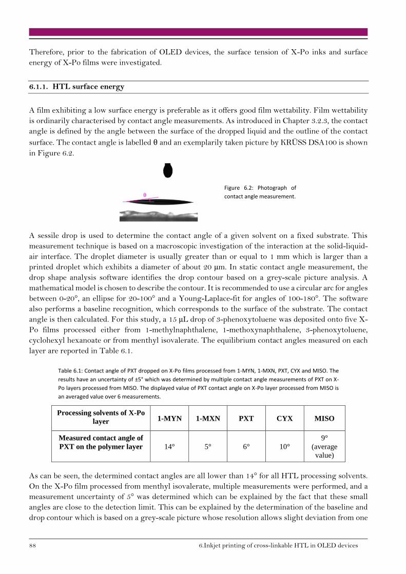
88 6.Inkjet printing of cross-linkable HTL in OLED devices
Therefore, prior to the fabrication of OLED devices, the surface tension of X-Po inks and surface
energy of X-Po films were investigated.
6.1.1. HTL surface energy
A film exhibiting a low surface energy is preferable as it offers good film wettability. Film wettability
is ordinarily characterised by contact angle measurements. As introduced in Chapter 3.2.3, the contact
angle is defined by the angle between the surface of the dropped liquid and the outline of the contact
surface. The contact angle is labelled θ and an exemplarily taken picture by KRÜSS DSA100 is shown
in Figure 6.2.
Figure 6.2: Photograph of
contact angle measurement.
A sessile drop is used to determine the contact angle of a given solvent on a fixed substrate. This
measurement technique is based on a macroscopic investigation of the interaction at the solid-liquid-
air interface. The droplet diameter is usually greater than or equal to 1 mm which is larger than a
printed droplet which exhibits a diameter of about 20 µm. In static contact angle measurement, the
drop shape analysis software identifies the drop contour based on a grey-scale picture analysis. A
mathematical model is chosen to describe the contour. It is recommended to use a circular arc for angles
between 0-20°, an ellipse for 20-100° and a Young-Laplace-fit for angles of 100-180°. The software
also performs a baseline recognition, which corresponds to the surface of the substrate. The contact
angle is then calculated. For this study, a 15 µL drop of 3-phenoxytoluene was deposited onto five X-
Po films processed either from 1-methylnaphthalene, 1-methoxynaphthalene, 3-phenoxytoluene,
cyclohexyl hexanoate or from menthyl isovalerate. The equilibrium contact angles measured on each
layer are reported in Table 6.1.
Table 6.1: Contact angle of PXT dropped on X-Po films processed from 1-MYN, 1-MXN, PXT, CYX and MISO. The
results have an uncertainty of ±5° which was determined by multiple contact angle measurements of PXT on X-
Po layers processed from MISO. The displayed value of PXT contact angle on X-Po layer processed from MISO is
an averaged value over 6 measurements.
Processing solvents of X-Po
layer 1-MYN 1-MXN PXT CYX MISO
Measured contact angle of
PXT on the polymer layer 14° 5° 6° 10°
9°
(average
value)
As can be seen, the determined contact angles are all lower than 14° for all HTL processing solvents.
On the X-Po film processed from menthyl isovalerate, multiple measurements were performed, and a
measurement uncertainty of 5° was determined which can be explained by the fact that these small
angles are close to the detection limit. This can be explained by the determination of the baseline and
drop contour which is based on a grey-scale picture whose resolution allows slight deviation from one
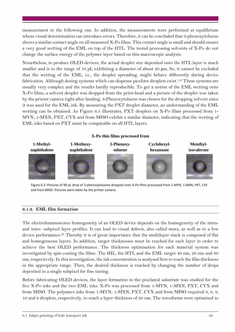
6.1. Inkjet printing of hole transport ink 89
measurement to the following one. In addition, the measurements were performed at equilibrium
whose visual determination can introduce errors. Therefore, it can be concluded that 3-phenoxytoluene
shows a similar contact angle on all measured X-Po films. This contact angle is small and should ensure
a very good wetting of the EML on top of the HTL. The tested processing solvents of X-Po do not
change the surface energy of the polymer layer based on this macroscopic analysis.
Nonetheless, to produce OLED devices, the actual droplet size deposited onto the HTL layer is much
smaller and is in the range of 10 pL exhibiting a diameter of about 20 µm. So, it cannot be excluded
that the wetting of the EML, i.e., the droplet spreading, might behave differently during device
fabrication. Although dosing systems which can dispense picolitre droplets exist.143 These systems are
usually very complex and the results hardly reproducible. To get a notion of the EML wetting onto
X-Po films, a solvent droplet was dropped from the print-head and a picture of the droplet was taken
by the printer camera right after landing. 3-Phenoxytoluene was chosen for the dropping solvent since
it was used for the EML ink. By measuring the PXT droplet diameter, an understanding of the EML
wetting can be obtained. As Figure 6.3 illustrates, PXT droplets on X-Po films processed from 1-
MYN, 1-MXN, PXT, CYX and from MISO exhibit a similar diameter, indicating that the wetting of
EML inks based on PXT must be comparable on all HTL layers.
Figure 6.3: Pictures of 90 pL drop of 3-phenoxytoluene dropped onto X-Po films processed from 1-MYN, 1-MXN, PXT, CYX
and from MISO. Pictures were taken by the printer camera.
6.1.2. EML film formation
The electroluminescence homogeneity of an OLED device depends on the homogeneity of the intra-
and inter- subpixel layer profiles. It can lead to visual defects, also called mura, as well as to a low
device performance.98 Thereby it is of great importance that the multilayer stack is composed of flat
and homogeneous layers. In addition, target thicknesses must be reached for each layer in order to
achieve the best OLED performance. The thickness optimisation for each material system was
investigated by spin coating the films. The HIL, the HTL and the EML target 40 nm, 20 nm and 80
nm, respectively. In this investigation, the ink concentration is analysed first to reach the film thickness
in the appropriate range. Then, the desired thickness is reached by changing the number of drops
deposited in a single subpixel for fine tuning.
Before fabricating OLED devices, the layer formation in the pixelated substrate was studied for the
five X-Po inks and the two EML inks. X-Po was processed from 1-MYN, 1-MXN, PXT, CYX and
from MISO. The polymers inks from 1-MYN, 1-MXN, PXT, CYX and from MISO required 8, 9, 8,
10 and 9 droplets, respectively, to reach a layer thickness of 20 nm. The waveforms were optimised to
X-Po thin films processed from
1-Methyl-
naphthalene
1-Methoxy-
naphthalene
3-Phenoxy-
toluene
Cyclohexyl-
hexanoate
Menthyl-
isovalerate

90 6.Inkjet printing of cross-linkable HTL in OLED devices
jet droplets of 10 pL (±1 pL) reaching a speed of 4-5 m∙s-1. The EML was processed from PXT and
from MISO. To investigate film profile formation in subpixels, profilometry was used as described in
Chapter 3.2.3.
Figure 6.4: Schematic of the profilometer needle scanning
a substrate exhibiting a substantial height change that can
be assimilated to the subpixel banks. The needle is drawn
at various times of a scan.
One artefact was observed by scanning a substantial height change at the bank sides. The needle scans
a surface at a constant speed. When the needle reaches a substantial height reduction, the needle keeps
moving in the scanning direction while reducing its height to reach the surface in the lower height. As
a consequence, the measured profile on the left side of the bank shows a smooth and curved height
changed as depicted in Figure 6.4, instead of revealing the sharp height change. On the opposite, when
the needle meets a substantial height increase, the needle first hits the edge and then the height is
adjusted while keeping a contact to the edge. Thus, in this configuration, the right side of the bank is
better resolved.
Figure 6.5: HIL, HTL and EML layers profiles measured by
profilometer in a subpixel. The HIL is common to all
subpixels. The HTL was printed from (a) 1-MYN, (b) 1-MXN,
(c) PXT, (d) CYX and (e) MISO. The EML was processed from
PXT in all subpixels. The active area of a subpixel is depicted
by a blue arrow in (a). The HIL, the HTL and the EML were
printed to reach 40 nm, 20 nm and 80 nm, respectively, in
the centre of the subpixels.
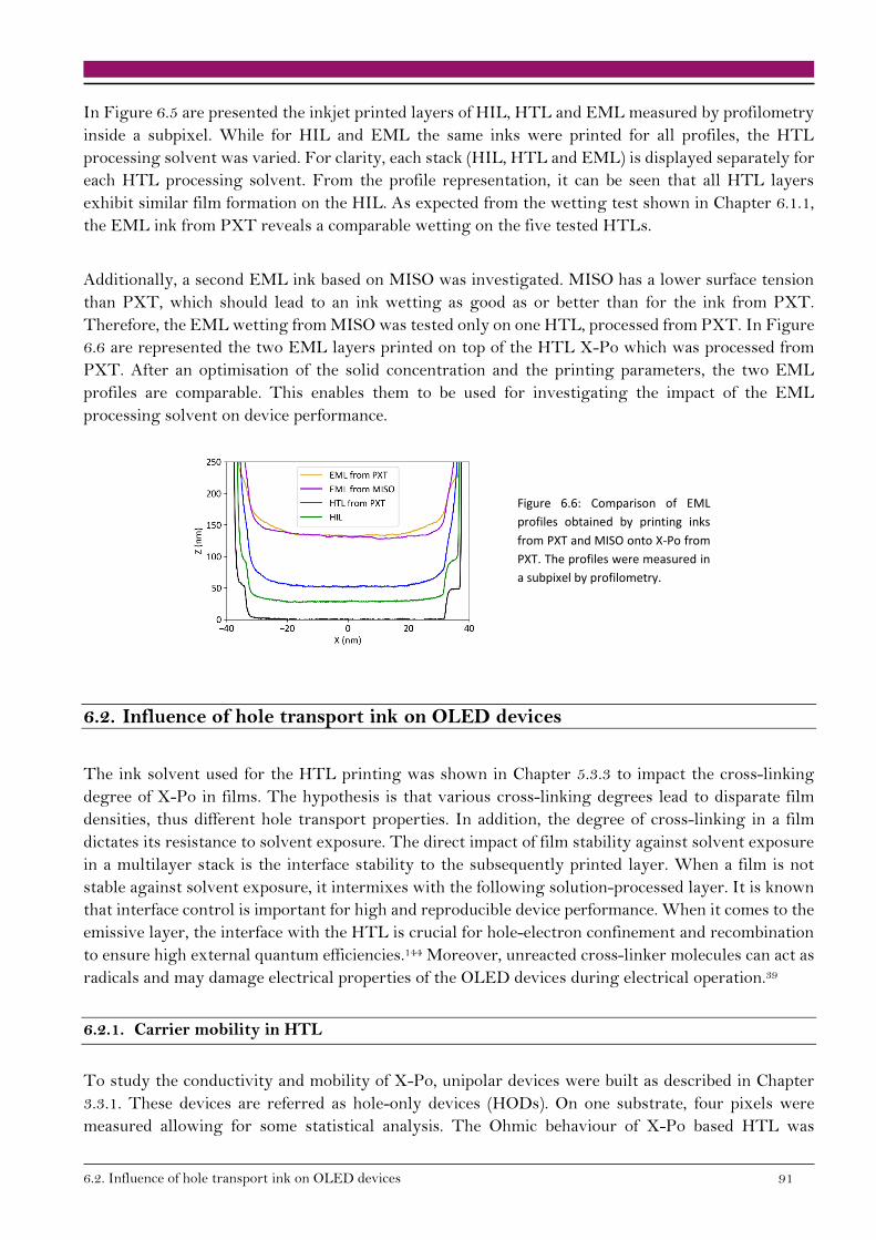
6.2. Influence of hole transport ink on OLED devices 91
In Figure 6.5 are presented the inkjet printed layers of HIL, HTL and EML measured by profilometry
inside a subpixel. While for HIL and EML the same inks were printed for all profiles, the HTL
processing solvent was varied. For clarity, each stack (HIL, HTL and EML) is displayed separately for
each HTL processing solvent. From the profile representation, it can be seen that all HTL layers
exhibit similar film formation on the HIL. As expected from the wetting test shown in Chapter 6.1.1,
the EML ink from PXT reveals a comparable wetting on the five tested HTLs.
Additionally, a second EML ink based on MISO was investigated. MISO has a lower surface tension
than PXT, which should lead to an ink wetting as good as or better than for the ink from PXT.
Therefore, the EML wetting from MISO was tested only on one HTL, processed from PXT. In Figure
6.6 are represented the two EML layers printed on top of the HTL X-Po which was processed from
PXT. After an optimisation of the solid concentration and the printing parameters, the two EML
profiles are comparable. This enables them to be used for investigating the impact of the EML
processing solvent on device performance.
Figure 6.6: Comparison of EML
profiles obtained by printing inks
from PXT and MISO onto X-Po from
PXT. The profiles were measured in
a subpixel by profilometry.
6.2. Influence of hole transport ink on OLED devices
The ink solvent used for the HTL printing was shown in Chapter 5.3.3 to impact the cross-linking
degree of X-Po in films. The hypothesis is that various cross-linking degrees lead to disparate film
densities, thus different hole transport properties. In addition, the degree of cross-linking in a film
dictates its resistance to solvent exposure. The direct impact of film stability against solvent exposure
in a multilayer stack is the interface stability to the subsequently printed layer. When a film is not
stable against solvent exposure, it intermixes with the following solution-processed layer. It is known
that interface control is important for high and reproducible device performance. When it comes to the
emissive layer, the interface with the HTL is crucial for hole-electron confinement and recombination
to ensure high external quantum efficiencies.144 Moreover, unreacted cross-linker molecules can act as
radicals and may damage electrical properties of the OLED devices during electrical operation.39
6.2.1. Carrier mobility in HTL
To study the conductivity and mobility of X-Po, unipolar devices were built as described in Chapter
3.3.1. These devices are referred as hole-only devices (HODs). On one substrate, four pixels were
measured allowing for some statistical analysis. The Ohmic behaviour of X-Po based HTL was

92 6.Inkjet printing of cross-linkable HTL in OLED devices
examined at low voltage and low current densities. In the Ohmic regime a variation in the current
density of 2 to 3 orders of magnitude was found between three pixels of the same substrate. In this case
the X-Po layer was processed from 1-MXN and annealed at 225°C, the current density changed from
0.002 mA∙cm-2 to 0.2 mA∙cm-2 at 1V, as can be seen in Figure 6.7. It means that the measured pixels of
the same material, the same fabrication process, the same solvent produce strongly divergent J-V
characteristics in the Ohmic regime. This very low reproducibility can be explained by leakage of the
HTL layer leading to a low intrinsic conductivity. Physically that means that at low voltages the
conductivity, defined as 𝜎 = 𝑒𝑛µ, changes by two orders of magnitude. Here 𝑒 is the elementary
charge, 𝑛 the charge carrier density and µ the charge carrier mobility. The origin of this leakage can
be manifold: easy possibilities can be seen in the existence of pinholes which upon metallisation lead to
conductive metallic whiskers through the layers or in the presence of chemical dopants through
residual impurities in the utilised polymer and solvents.
Figure 6.7: Current density vs voltage
characteristics of HODs. The devices were built
from 40 nm HIL films / HTL of 35 nm X-Po films
from 1-MXN. The curves of the pixels (A in
purple, B in red, C in cyan) and the linear fitting
of n=1 are plotted on double logarithmic scales.
In order to reach the quadratic regime of space-charge-limited currents in the trap free regime, high
voltages of up to 10V were applied to the HOD to use the Mott-Gurney law to determine the charge
carrier mobility µ of the HTL. Unfortunately, in all reported I-V characteristics it was not possible to
reach the required SCLC regime which prohibits the determination of the charge carrier mobility. The
reason for not reaching the quadratic regime of the I-V curves is the existence of deep traps which are
responsible for the steep increase in the I-V-characteristics following Ohm’s regime.145 Direct
interpretation of the current–voltage characteristics, however, is difficult due to the absence of
knowledge on the energetical trap distribution as well as on the injection and extraction barriers of the
involved layers.146
6.2.2. Bipolar devices
Bipolar devices have a complex multilayer architecture and were built as presented in Chapter 3.3.2
using a green dye in the EML. It can be challenging to analyse the performance of bipolar devices since
their different materials and interfaces are influencing device properties like luminous efficiency and
device lifetime. Therefore, it was ensured that only such devices were compared, which differ from each
other by only one parameter, allowing a reliable and straightforward analysis.
The bipolar devices fabricated in this doctoral work were aimed at reviewing the HTL/EML interface.
Critical for luminous efficiency35 and device lifetime, this interface can be influenced by various
parameters including material for the HTL, the corresponding HTL ink solvent, the HTL annealing
temperature, the materials for the EML, the EML ink solvent, the drying time, etc. Thereby it is

6.2. Influence of hole transport ink on OLED devices 93
important to control and understand the interfacial structures of the multilayers because it is
considered important to improve the OLED characteristics.147 In order to pronounce the impact of the
HTL/EML interface, the OLED devices were built so that the recombination zone is localised close
to the HTL/EML interface. The OLED stack development to obtain the recombination zone next to
the HTL/EML interface is the result of other people’s work.148
HTL annealing temperature
X-Po is a cross-linkable polymer whose cross-linking reaction is activated by thermal energy. To
investigate the impact of the cross-linking degree of the X-Po based HTL on OLED performance, the
HTL was annealed at various temperatures for 30 minutes on a hotplate and tested in bipolar devices.
The temperature range was chosen between 160°C and 260°C around the reference temperature of
225°C (explained in Chapter 5.3.2). In this investigation, the HTL was processed from PXT, a solvent
exhibiting a medium strong interaction with the polymer in comparison to the other studied solvents
of this work (see Chapter 4.1). The EML was also processed from PXT, which shows as a pure solvent
also a medium deformation of the underlying HTL also processed from PXT (see Chapter 5.3.2).
Figure 6.8: Bipolar OLED devices performance with
EML processed from PXT. Object of the study is the HTL
annealing temperature. (a) J-V characteristics of OLED
devices as a function of the HTL annealing
temperature. (b) Efficiencies of OLED devices with HTL
annealed at various temperatures. (c) Luminance
lifetimes of OLED devices with HTL annealed at various
temperatures.
The influence of the HTL annealing temperature on OLED luminous efficiency, J-V characteristics
and device lifetime performance is displayed in Figure 6.8. Devices comprising the HTL annealed at
160°C and at 180°C reveal the highest current densities of 100 mA∙cm-2 at 10.4 V. As the HTL
annealing temperature is increased from 180°C to 260°C, the driving voltage increases, as can be seen
in Figure 6.8a. Devices with the HTL annealed at 260°C reach 100 mA∙cm-2 at 16.5 V. A possible
explanation can be seen either by changes in the hole transport properties, e.g., hole mobility of the
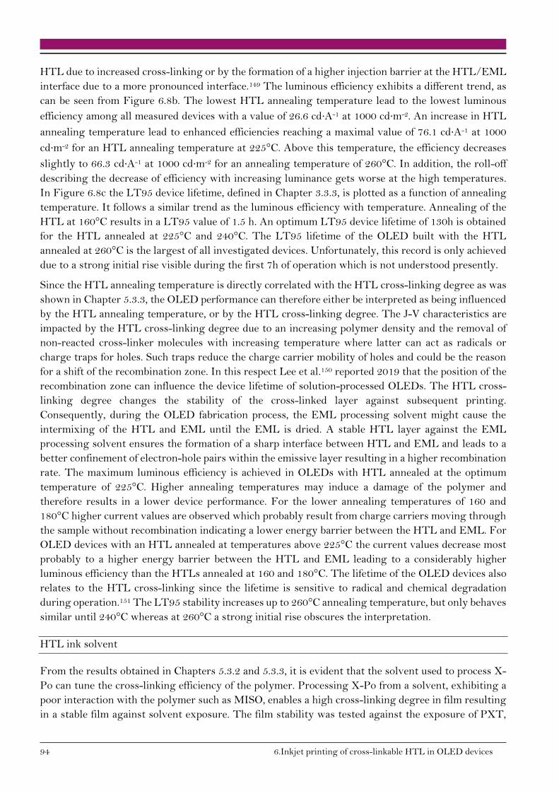
94 6.Inkjet printing of cross-linkable HTL in OLED devices
HTL due to increased cross-linking or by the formation of a higher injection barrier at the HTL/EML
interface due to a more pronounced interface.149 The luminous efficiency exhibits a different trend, as
can be seen from Figure 6.8b. The lowest HTL annealing temperature lead to the lowest luminous
efficiency among all measured devices with a value of 26.6 cd∙A-1 at 1000 cd∙m-2. An increase in HTL
annealing temperature lead to enhanced efficiencies reaching a maximal value of 76.1 cd∙A-1 at 1000
cd∙m-2 for an HTL annealing temperature at 225°C. Above this temperature, the efficiency decreases
slightly to 66.3 cd∙A-1 at 1000 cd∙m-2 for an annealing temperature of 260°C. In addition, the roll-off
describing the decrease of efficiency with increasing luminance gets worse at the high temperatures.
In Figure 6.8c the LT95 device lifetime, defined in Chapter 3.3.3, is plotted as a function of annealing
temperature. It follows a similar trend as the luminous efficiency with temperature. Annealing of the
HTL at 160°C results in a LT95 value of 1.5 h. An optimum LT95 device lifetime of 130h is obtained
for the HTL annealed at 225°C and 240°C. The LT95 lifetime of the OLED built with the HTL
annealed at 260°C is the largest of all investigated devices. Unfortunately, this record is only achieved
due to a strong initial rise visible during the first 7h of operation which is not understood presently.
Since the HTL annealing temperature is directly correlated with the HTL cross-linking degree as was
shown in Chapter 5.3.3, the OLED performance can therefore either be interpreted as being influenced
by the HTL annealing temperature, or by the HTL cross-linking degree. The J-V characteristics are
impacted by the HTL cross-linking degree due to an increasing polymer density and the removal of
non-reacted cross-linker molecules with increasing temperature where latter can act as radicals or
charge traps for holes. Such traps reduce the charge carrier mobility of holes and could be the reason
for a shift of the recombination zone. In this respect Lee et al.150 reported 2019 that the position of the
recombination zone can influence the device lifetime of solution-processed OLEDs. The HTL cross-
linking degree changes the stability of the cross-linked layer against subsequent printing.
Consequently, during the OLED fabrication process, the EML processing solvent might cause the
intermixing of the HTL and EML until the EML is dried. A stable HTL layer against the EML
processing solvent ensures the formation of a sharp interface between HTL and EML and leads to a
better confinement of electron-hole pairs within the emissive layer resulting in a higher recombination
rate. The maximum luminous efficiency is achieved in OLEDs with HTL annealed at the optimum
temperature of 225°C. Higher annealing temperatures may induce a damage of the polymer and
therefore results in a lower device performance. For the lower annealing temperatures of 160 and
180°C higher current values are observed which probably result from charge carriers moving through
the sample without recombination indicating a lower energy barrier between the HTL and EML. For
OLED devices with an HTL annealed at temperatures above 225°C the current values decrease most
probably to a higher energy barrier between the HTL and EML leading to a considerably higher
luminous efficiency than the HTLs annealed at 160 and 180°C. The lifetime of the OLED devices also
relates to the HTL cross-linking since the lifetime is sensitive to radical and chemical degradation
during operation.151 The LT95 stability increases up to 260°C annealing temperature, but only behaves
similar until 240°C whereas at 260°C a strong initial rise obscures the interpretation.
HTL ink solvent
From the results obtained in Chapters 5.3.2 and 5.3.3, it is evident that the solvent used to process X-
Po can tune the cross-linking efficiency of the polymer. Processing X-Po from a solvent, exhibiting a
poor interaction with the polymer such as MISO, enables a high cross-linking degree in film resulting
in a stable film against solvent exposure. The film stability was tested against the exposure of PXT,
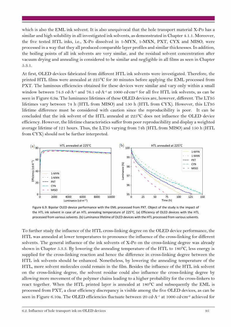
6.2. Influence of hole transport ink on OLED devices 95
which is also the EML ink solvent. It is also unequivocal that the hole transport material X-Po has a
similar and high solubility in all investigated ink solvents, as demonstrated in Chapter 4.1.1. Moreover,
the five tested HTL inks, i.e., X-Po dissolved in 1-MYN, 1-MXN, PXT, CYX and MISO, were
processed in a way that they all produced comparable layer profiles and similar thicknesses. In addition,
the boiling points of all ink solvents are very similar, and the residual solvent concentration after
vacuum drying and annealing is considered to be similar and negligible in all films as seen in Chapter
5.3.1.
At first, OLED devices fabricated from different HTL ink solvents were investigated. Therefore, the
printed HTL films were annealed at 225°C for 30 minutes before applying the EML processed from
PXT. The luminous efficiencies obtained for these devices were similar and vary only within a small
window between 74.3 cd∙A-1 and 76.1 cd∙A-1 at 1000 cd∙cm-2 for all five HTL ink solvents, as can be
seen in Figure 6.9a. The luminance lifetimes of these OLED devices are, however, different. The LT95
lifetimes vary between 74 h (HTL from MISO) and 150 h (HTL from CYX). However, this LT95
lifetime difference must be considered with caution since the reproducibility is poor. It can be
concluded that the ink solvent of the HTL annealed at 225°C does not influence the OLED device
efficiency. However, the lifetime characteristics suffer from poor reproducibility and display a weighted
average lifetime of 121 hours. Thus, the LT95 varying from 74h (HTL from MISO) and 150 h (HTL
from CYX) should not be further interpreted.
Figure 6.9: Bipolar OLED device performance with the EML processed from PXT. Object of the study is the impact of
the HTL ink solvent in case of an HTL annealing temperature of 225°C. (a) Efficiency of OLED devices with the HTL
processed from various solvents. (b) Luminance lifetime of OLED devices with the HTL processed from various solvents.
To further study the influence of the HTL cross-linking degree on the OLED device performance, the
HTL was annealed at lower temperatures to pronounce the influence of the cross-linking for different
solvents. The general influence of the ink solvents of X-Po on the cross-linking degree was already
shown in Chapter 5.3.3. By lowering the annealing temperature of the HTL to 180°C, less energy is
supplied for the cross-linking reaction and hence the difference in cross-linking degree between the
HTL ink solvents should be enhanced. Nonetheless, by lowering the annealing temperature of the
HTL, more solvent molecules could remain in the film. Besides the influence of the HTL ink solvent
on the cross-linking degree, the solvent residue could also influence the cross-linking degree by
allowing more movement of the polymer chains leading to a higher probability for the cross-linkers to
react together. When the HTL printed layer is annealed at 180°C and subsequently the EML is
processed from PXT, a clear efficiency discrepancy is visible among the five OLED devices, as can be
seen in Figure 6.10a. The OLED efficiencies fluctuate between 20 cd∙A-1 at 1000 cd∙cm-2 achieved for

96 6.Inkjet printing of cross-linkable HTL in OLED devices
the device with the HTL processed from 1-MYN and 63 cd∙A-1 at 1000 cd∙cm-2 achieved with the HTL
processed from MISO. Likewise, the OLED lifetimes exhibit a distinctive divergence among the five
OLED devices. The LT95 lifetimes vary from 1 hour achieved for the device with the HTL processed
from 1-MYN to 40 hours achieved for the device with the HTL processed from MISO.
Figure 6.10: OLED performance in case of the EML being processed from PXT. Object of the study is to understand the
impact of the HTL ink solvent when the HTL is annealed at 180°C. (a) Efficiency and (b) lifetimes of OLEDs in dependence
of the HTL processing solvent as indicated.
For the solvents 1-MYN, PXT and MISO a correlation between the polymer-solvent interactions and
the device performances can be drawn. It was shown that there exists a very strong polymer-solvent
interaction between 1-MYN and X-Po meaning that 1-MYN is a good solvent for X-Po. This strong
binding between 1-MYN and X-Po hinders a strong densification of the polymer chains and therewith
the cross-linking. The result is a low efficiency and a low LT95 lifetime. This is different for the device
with HTL processed from MISO. In this case MISO is a poor solvent and the binding of the solvent
to the X-Po is weak and can be destroyed even at low temperatures. This leads to a strong densification
and an efficient cross-linking. For MISO the efficiency is high and the LT95 lifetime is the longest.
The other three solvents show intermediate behaviour in all respects: binding, efficiency and LT95.
The results for the stronger binding solutions of X-Po with 1-MXN, PXT, CYX and MISO exhibit an
increasing cross-linking degree and explain an increased film stability against solvent exposure
probably resulting in a pronounced HTL/EML interface, a higher stability and a larger efficiency.
EML processing solvent
In this part of the thesis, interface conditions were interpreted in terms of stability of the HTL against
a subsequently solution-processed EML on top of it. Interface stability can thereby be described as the
capability to solution-process a subsequent layer without damaging the previous one. Besides the use
of a cross-linked HTL, HTL stability against a solution-processed EML can also be achieved by the
use of an EML solvent which shows a poor interaction with the HTL.21-22, 152 Processing the EML
from a poor solvent for the HTL polymer results in the absence of interaction between the EML
solvent and the X-Po film while the EML is wet. In Chapter 4.1 it was confirmed that MISO is the
solvent having the worst affinity with X-Po within the set of tested solvents. Nevertheless, MISO
provides solubility enabling the dissolution of the emissive material at a concentration of 25 g∙L-1,
which is sufficient to establish a target thickness of 80 nm in OLED devices in one printing step.
In Figure 6.11, the OLED performances of four devices are displayed. After processing the HIL X-Po
was printed from 1-MYN, CYX, PXT and MISO. All HTLs were vacuum dried and annealed at 180°C
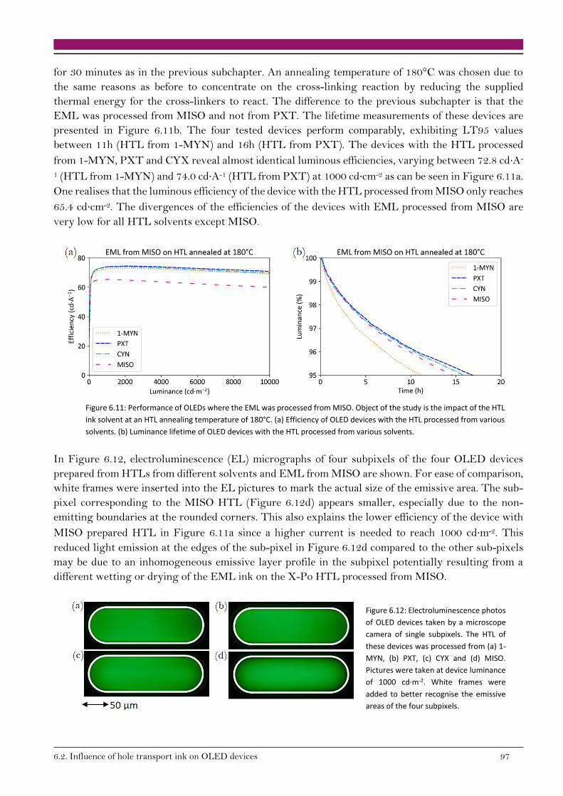
6.2. Influence of hole transport ink on OLED devices 97
for 30 minutes as in the previous subchapter. An annealing temperature of 180°C was chosen due to
the same reasons as before to concentrate on the cross-linking reaction by reducing the supplied
thermal energy for the cross-linkers to react. The difference to the previous subchapter is that the
EML was processed from MISO and not from PXT. The lifetime measurements of these devices are
presented in Figure 6.11b. The four tested devices perform comparably, exhibiting LT95 values
between 11h (HTL from 1-MYN) and 16h (HTL from PXT). The devices with the HTL processed
from 1-MYN, PXT and CYX reveal almost identical luminous efficiencies, varying between 72.8 cd∙A-
1 (HTL from 1-MYN) and 74.0 cd∙A-1 (HTL from PXT) at 1000 cd∙cm-2 as can be seen in Figure 6.11a.
One realises that the luminous efficiency of the device with the HTL processed from MISO only reaches
65.4 cd∙cm-2. The divergences of the efficiencies of the devices with EML processed from MISO are
very low for all HTL solvents except MISO.
Figure 6.11: Performance of OLEDs where the EML was processed from MISO. Object of the study is the impact of the HTL
ink solvent at an HTL annealing temperature of 180°C. (a) Efficiency of OLED devices with the HTL processed from various
solvents. (b) Luminance lifetime of OLED devices with the HTL processed from various solvents.
In Figure 6.12, electroluminescence (EL) micrographs of four subpixels of the four OLED devices
prepared from HTLs from different solvents and EML from MISO are shown. For ease of comparison,
white frames were inserted into the EL pictures to mark the actual size of the emissive area. The sub-
pixel corresponding to the MISO HTL (Figure 6.12d) appears smaller, especially due to the non-
emitting boundaries at the rounded corners. This also explains the lower efficiency of the device with
MISO prepared HTL in Figure 6.11a since a higher current is needed to reach 1000 cd∙m-2. This
reduced light emission at the edges of the sub-pixel in Figure 6.12d compared to the other sub-pixels
may be due to an inhomogeneous emissive layer profile in the subpixel potentially resulting from a
different wetting or drying of the EML ink on the X-Po HTL processed from MISO.
Figure 6.12: Electroluminescence photos
of OLED devices taken by a microscope
camera of single subpixels. The HTL of
these devices was processed from (a) 1-
MYN, (b) PXT, (c) CYX and (d) MISO.
Pictures were taken at device luminance
of 1000 cd∙m-2. White frames were
added to better recognise the emissive
areas of the four subpixels.
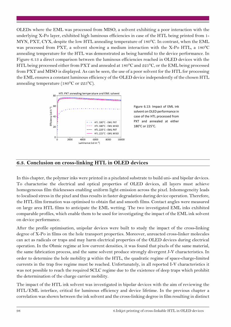
98 6.Inkjet printing of cross-linkable HTL in OLED devices
OLEDs where the EML was processed from MISO, a solvent exhibiting a poor interaction with the
underlying X-Po layer, exhibited high luminous efficiencies in case of the HTL being printed from 1-
MYN, PXT, CYX, despite the low HTL annealing temperature of 180°C. In contrast, when the EML
was processed from PXT, a solvent showing a medium interaction with the X-Po HTL, a 180°C
annealing temperature for the HTL was demonstrated as being harmful to the device performance. In
Figure 6.13 a direct comparison between the luminous efficiencies reached in OLED devices with the
HTL being processed either from PXT and annealed at 180°C and 225°C, or the EML being processed
from PXT and MISO is displayed. As can be seen, the use of a poor solvent for the HTL for processing
the EML ensures a constant luminous efficiency of the OLED device independently of the chosen HTL
annealing temperature (180°C or 225°C).
Figure 6.13: Impact of EML ink
solvent on OLED performance in
case of the HTL processed from
PXT and annealed at either
180°C or 225°C.
6.3. Conclusion on cross-linking HTL in OLED devices
In this chapter, the polymer inks were printed in a pixelated substrate to build uni- and bipolar devices.
To characterise the electrical and optical properties of OLED devices, all layers must achieve
homogeneous film thicknesses enabling uniform light emission across the pixel. Inhomogeneity leads
to localised stress in the pixel and thus results in faster degradation during device operation. Therefore,
the HTL film formation was optimised to obtain flat and smooth films. Contact angles were measured
on large area HTL films to anticipate the EML wetting. The two investigated EML inks exhibited
comparable profiles, which enable them to be used for investigating the impact of the EML ink solvent
on device performance.
After the profile optimisation, unipolar devices were built to study the impact of the cross-linking
degree of X-Po in films on the hole transport properties. Moreover, unreacted cross-linker molecules
can act as radicals or traps and may harm electrical properties of the OLED devices during electrical
operation. In the Ohmic regime at low current densities, it was found that pixels of the same material,
the same fabrication process, and the same solvent produce strongly divergent J-V characteristics. In
order to determine the hole mobility µ within the HTL, the quadratic regime of space-charge-limited
currents in the trap free regime must be reached. Unfortunately, in all reported I-V characteristics it
was not possible to reach the required SCLC regime due to the existence of deep traps which prohibit
the determination of the charge carrier mobility.
The impact of the HTL ink solvent was investigated in bipolar devices with the aim of reviewing the
HTL/EML interface, critical for luminous efficiency and device lifetime. In the previous chapter a
correlation was shown between the ink solvent and the cross-linking degree in film resulting in distinct
6.3. Conclusion on cross-linking HTL in OLED devices 99
film stabilities against specific solvent exposure. The direct impact of film stability against solvent
exposure in a multilayer stack was the interface stability to the subsequently printed layer. When a
film was not stable against solvent exposure, it intermixed with the following solution-processed layer.
It was shown that the cross-linking degree can be varied by the annealing temperature; the higher the
annealing temperature, the higher was the cross-linking degree. The maximum luminous efficiency
was achieved in OLEDs for HTL annealed at the optimum temperature of 225°C. Higher annealing
temperatures induce damage to the polymer or to the other layers and therefore resulted in a lower
device performance. On the other hand, lower annealing temperatures exhibited higher current
densities explained by lower energy barriers between the HTL and EML. The lifetime of the OLED
devices also related to the HTL cross-linking degree since the lifetime is sensitive to radical and
chemical degradation during operation. The cross-linking degree was shown to considerably influence
the luminous efficiency of OLED devices. The second attempt to enhance the cross-linking degree was
performed by varying the HTL ink solvent. It was shown that the ink solvent of the HTL annealed at
225°C did not influence the OLED device efficiency. To deeper understand the cross-linking
conditions, the HTL were annealed at 180°C, where less energy was available for the cross-linking
reaction to occur. In this case HTLs processed from poor solvents exhibited higher luminous efficiency
and a longer lifetime than HTL processed from good solvent. This can be explained by the high cross-
linking degree reached in film from poor solvents resulting in an energetically steeper HTL/EML
interface, a higher stability and a larger efficiency. Finally, OLED devices were built where the EML
was processed from a solvent exhibiting a poor interaction with the underlying X-Po layer. A stable
HTL/EML interface was expected since no interaction should occur between the subsequent solution-
processed films. Higher luminous efficiencies were attained when the HTL was annealed at 180°C and
when the EML was processed from a solvent showing a poor interaction with X-Po than when
processed from a solvent with a medium interaction with X-Po.
The HTL ink solvent was demonstrated to have a strong influence on OLED device performance when
the HTL was annealed at 180°C. Poor solvent insured a stable HTL against subsequent EML printing
resulting in high luminous efficiency and longer lifetime. In addition, the EML ink solvent was shown
to impact the OLED efficiency. Processing the EML from a solvent showing a poor interaction with
the HTL improved the device performance when the HTL was annealed at 180°C.
In this chapter, it was shown that the hole conductivity within the HTL suffered from low
reproducibility. Due to deep traps, the determination of the hole mobility was not achieved through I-
V characteristics of unipolar devices. An annealing temperature of 180°C was used for the HTL to
demonstrate the impact of the HTL polymer-solvent affinity on the electrical properties of bipolar
devices. HTL processed from poor solvent exhibited higher luminous efficiencies and longer lifetimes
than HTL processed from good solvent. The same was found for the EML, where higher luminous
efficiencies were achieved when the EML was processed from a solvent showing a poor interaction
with the HTL.

7.Summary 101
7. Summary
Interfaces, their definition, characterisation and controlled generation are studied intensively in
various semiconductor devices having a multilayer architecture. Furthermore, not only in OLEDs, but
also in OPVs and OFETs, solution processes are attractive in research laboratories and on the market.
To ensure a stable layer against a subsequently solution-processed layer, various methods have been
reviewed in the literature. This thesis focused on the use of cross-linked polymers, with a styrene cross-
linker whose reaction is thermally triggered. To process this material, inkjet printing is the method of
choice since it is a promising technology for high resolution displays. The aim of this work was to
examine the influence of the ink solvent on the layer stability against subsequent printing and its
impact on OLED device performance.
Prior to the investigation of the polymer ink and the resulting layers, a set of five solvents suiting the
inkjet printing process was defined covering the relevant parameter space of surface tension, viscosity
and boiling point. The solvents were described by the interaction with the investigated polymer X-Po.
That way, the learnings can be applied to any set of material and solvent by a simple interaction
characterisation. The affinity of X-Po with the ink solvent was characterised by experiments as well
as empirical observations based on the Mark-Houwink parameters, the Huggins and Kramer constants,
and the Solomon Ciuta equation. The intrinsic values of X-Po in the five tested solvents varied between
0.61 and 0.74 L∙g-1 which due to their similarity hinders the identification of a preferred solvent for X-
Po. On the opposite, Huggins and Kraemer constants identified 1-MYN as good solvent for X-Po, and
PXT, CYX and MISO as poor solvents for X-Po. To enhance this differentiation among the five
solvents, an experimental setup was developed based on the non-solvent induced phase separation
(NIPS) method. By this developed technique, the strength of interaction between the polymer and the
solvents were classified from the strongest to the weakest as: 1-MYN, 1-MXN, PXT, CYX and MISO.
The trend observed by Huggins and Kraemer constants is in agreement with the experimental result
of polymer-solvent interactions. Flory and Fox as well as Einstein equation revealed a similar radius
of gyration of X-Po in the five solvents of 1.3 nm (±0.8 nm). DLS measurements could not
experimentally confirm or disconfirm these results since experimental limitations were met at low
concentration and unfortunately no relevant signal could be detected.
The styrene cross-linking reaction mechanism, already reported in patents,126 was characterised in this
work by DSC and FTIR. Due to the low content of styrene in the X-Po chain (10 %), direct analysis of
the X-Po IR absorption was inconclusive. An increase of the cross-linking group by a factor of seven
provided, however, a distinct understanding of the styrene cross-linking reaction and allowed for a
further interpretation of the X-Po cross-linking reaction. DSC turned out to be an appropriate method
to describe the exothermic reaction of styrene whose enthalpy attained 49 J∙g-1 and the maximum heat
flow was reached at 240°C.
Cross-linking was then studied in solution made from X-Po in 1-MYN, 1-MXN, PXT, CYX and MISO
at 50 g∙L-1 and was triggered by heating the solutions to different temperatures for three hours.
Rheology measurements were carried out to track the cross-linking reaction of X-Po in solution and
gave an evident indication of macroscopic changes. A heat treatment of 170°C and 180°C was enough
to cross-link the polymer solution prepared using MISO and CYX revealing a fast reaction in these
otherwise poor solvents. On the opposite, X-Po in 1-MYN and 1-MXN did not reveal any viscosity
102 7.Summary
variation independent of the temperature treatment. DSL measurements showed the presence of cross-
linked polymer chains where rheology could not identify viscosity variations thanks to its higher
sensitivity. The DLS results complemented the rheology measurements and a complete investigation
of the cross-linking reaction in solution at the nanoscale up to the macroscopic scale was possible. A
polymer solution prepared from a poor solvent cross-linked at lower temperature than a polymer
solution prepared from a good solvent.
The impact of ink solvent on the degree of cross-linking of X-Po measured by DSC was in accordance
with what was observed in solution and assessed by ink viscosity measurements. When processed from
a poor solvent, X-Po reached a higher cross-linking degree in film than a film processed from a good
solvent. The high cross-linking degree awarded the film of a stronger stability against further solvent
exposure. A direct correlation between ink solvent and thin film stability against solvent exposure was
identified. Polymer films processed from poor solvents exhibited a smaller deformation after solvent
exposure than polymer films of same thickness processed from good solvents for an otherwise identical
fabrication process. Thicker layers generally displayed a higher deformation than thinner layers of the
same material and ink solvent. The film deformation could also be influenced by the thermal annealing
process. A film annealed at higher temperature was more stable against solvent exposure.
To study the impact of ink solvent on the electronic properties of printed layers, uni- and bipolar
devices were processed. Hole-only devices were built to determine the charge mobility within an X-Po
HTL by space charge limited current (SCLC) techniques. In order to obtain reliable values for the
mobility the quadratic regime of the I-V characteristics of SCLC must be reached. Therefore, high
voltages were applied to the HODs. Unfortunately, the SCLC regime could not be attained. Light
emission obscured the HODs behaviour due to injection of negative charges from the cathode
destroying the conditions for SCLC. Therefore, the charge mobility within the HOD could not be
determined. Finally, bipolar OLED devices were printed from various HTL inks. For the solvents 1-
MYN, PXT and MISO, a correlation between the polymer-solvent interactions and the device
performances could be drawn. OLED devices fabricated with HTL processed from poor solvent resulted
in enhanced luminous efficiency as well as longer device lifetimes. This could be explained by an
increased film stability against solvent exposure guaranteeing a stable HTL/EML interface resulting
in a better confinement of electron-hole pairs within the emissive layer in favour of a higher
recombination rate.
The importance of IJP solvent choice to fabricate a stable cross-linked polymer film was successfully
demonstrated. This study demonstrates that the solvent selection is a critical parameter to enhance
the full potential of OLED materials in devices. Tuning the degree of cross-linking of a polymer thin
film resulting in different intermixing levels between successive layers is of general interest for
multilayer structures. The developed solvent exposure stability test is generally applicable and can be
of interest for other fields of activity, such as in the investigation of large area cross-linking
homogeneity.
8.Outlook 103
8. Outlook
As OLED device architectures become more and more complex, interface study and film properties
will remain a focus and additional steps will have to be taken to advance the research on that topic. Of
prime importance will be to evaluate the taken measures on a larger and even broader set of solvents,
in order to identify the limits of polymer-solvent interaction resulting in stable inks but also in
functional thin films. As an additional experimental technique to be used in the future, thin film stability
against solvent exposure as reported in literature could use atomic force microscopy (AFM). After
solvent exposure, morphology and layer thickness could be analysed to judge the efficiency of cross-
linking or orthogonal solvents by AFM.50 Also a mechanical characterisation by nanoindentation
through AFM could be used.153 Independently of the choice of the measurement method, further efforts
should aim on the influence of ink solvent on cross-linking efficiency in films or devices. Solvent
mixtures could be a next step toward a full understanding of the importance of solvent development
and choice for solution processes.
In this thesis, one limitation was met concerning the visualisation of the buried interface between two
layers. No depth profile was drawn along the multilayer stack to picture the learnings made by the
various experiments on the layer stability against subsequent printing. Interface visualisation was
demonstrated by various methods. Michael Bruns of Karlsruhe Institute of Technology presented a
technique to measure depth profile of atomic concentration by x-ray photoelectron spectroscopy
(XPS).154 Depth-profiling analysis was also performed by time-of-flight secondary ion mass
spectrometry (TOF-SIMS) involving ion beam etching.155 Evaluation of interfaces were reported using
neutron reflectometry (NR),156 impedance spectroscopy (IS) and ultraviolet photoelectron
spectroscopy (UPS).149 However, these methods require long measurement times inhibiting the
investigation of a large batch of samples. In addition, a strong attention should be brought to the
measurement resolution when thin films of a few tenths of nanometre are under investigation.
Ellipsometry is one possible measurement tool that can be employed to study interfaces in multilayer
stacks at the nanometre scale. A graded interface between two layers can be modelled and was reported
to be very accurate.157 For the application in OLEDs, further development should be done on
techniques with sub-nanometre resolution offering a fast analysis.
One of the fundamental problems with the orthogonal solvent system approach is that small-molecule
materials can be washed away by a solvent even though the small molecule might not be soluble in
that solvent. Recently, Aizawa et al.158 demonstrated that if the molecular weight of the small molecule
exceeds a certain threshold value, the film will remain intact. This work opens up a route to fabricate
small-molecule-based multilayer solution-processed OLEDs.159 Follow-up is needed in this direction
in order to build up multilayer architecture from solution with small molecules which are of interest
for high resolution displays. This path tackles interface control from the material instead of the ink
solvent point of view.


Acknowledgments 105
Acknowledgments
This thesis is the result of three years and ten months of experience I have encountered at the
Technische Universität Darmstadt and at Merck KGaA from various people who I wish to thank.
Firstly, I would like to extend my gratitude to the members of the committee, Prof. von Seggern, Prof.
Dörsam, Prof. Alff and Prof. Ensinger, for reading and accepting to assess this PhD thesis.
Prof. von Seggern, my Doktorvater, guided me throughout the research work which is why I would
like to express him my gratitude but also for his patience and persistent help with the writing of the
thesis. In addition, I wish to show my sincere appreciation to Prof. Dörsam, who welcomed me in his
research group and gave me constant encouragement throughout my research work. It was a great
chance to participate to the Doktorandkolloquium with the PhD students of the Institut für
Druckmaschinen und Druckverfahren (IDD) where insightful discussions took place.
I would also like to extend my deepest gratitude to Remi Anemian and Peter Levermore, who gave me
the opportunity to join the research team of OLED department in Merck Darmstadt. Without them,
this thesis would not have been possible. I am also pleased to say thank you to Edgar Böhm, Aurélie
Ludemann, Christian Heiss, Georg Bernatz and Rocco Fortte, who made my access simpler to the
research facilities and various laboratories.
I gratefully acknowledge the assistance of Katja Maria Scheible for re-orienting my research topic into
an exciting world exploring the impact of OLED ink formulation on material cross-linking properties.
Gaëlle Béalle have been and still is a tremendous mentor for me. I would like to thank you for always
being by my sides and for being a great advisor beyond imagination. During the challenging times,
you gave me confidence, moral support and the freedom I needed to grow as a research scientist. I
would also like to pay my special regards to Manuel Hamburger for his relentless support and profound
belief in my work and abilities to carry this academic study. I am extremely grateful for your patience
in the publication process of my article and your motivation that gave me power to excel in the research
writing.
The completion of my dissertation would not have been accomplished without the support of the Merck
OLED department. I express my deepest gratitude to the soluble team for playing a major role in my
research work and my personal development, especially Hsin-Rong Tseng, Sebastian Meyer, Sebastian
Stoltz and Miriam Engel.
Whenever possible, my days started in the best way around a coffee in the innovation center
surrounded by Bouchon, Stevi, Mikiki, Christoph and Manuel. I already missed this fruitful morning
discussions.
My fellow labmates played a decisive part in fulfilment of my goals and in keeping a good mental
health. A special thanks for the fun-time we spent together, and for the stimulating discussions. The
support of the OLED ink formulation and the OLED application printing team really meant a lot to

106 Acknowledgments
me. I was a great pleasure to work with you guys. Nathalie, Toto, Dieter, Chica, Denis and Thorsten,
I hope to cross your road again in a lab sometimes.
Heartfelt thanks to the labs and team that welcomed me for punctual measurements: the IDD team,
the first screening lab, the troubleshooting analytics lab, the early R&D formulation lab and the
analytical lab for particle characterisation.
I wish to express my sincere thanks to the support and love of my family and friends. My mädels, my
rainbow and Tac (from Tic&Tac) offered me a great cocktail encouragement and getaway moments
which I cherished. I feel the need to thank my parents in French…
Tima et tipa, vous êtes mes piliers, mon moteur et mon filet de sécurité. Vous me donnez l’amour et les moyens
nécessaires dont j’ai besoin pour accomplir tous mes projets, et je ne sais comment vous remercier. Je vous aime et
je continuerai à vous rendre fiers.
Last but not least, I thank Katim for entering my life during this exciting and challenging time. You
always believed in me, and you gave me wings.

Curriculum Vitae 107
Curriculum Vitae
Contact
Arheilger Weg 21
64331 Weiterstadt
Germany
+33 665-204897
Paulinehibon.51.45
Nationality: French
Social
https://www.linkedin.com/i
n/paulinehibon
Research gate
https://www.researchgate.net/pr
ofile/Pauline_Hibon
Education
PhD Thesis, Merck KGaA, TU Dar mstadt,
Dar mstadt (Ger many)
Influence of inkjet printing (IJP) solvents on cross-
linkable polymers thin films stability
• Formulation of IJP inks for OLED devices
• Characterisation of thin films
• Large area printing
5/2016 – Present
Master Thesis, Fraunhofer Institute IOF,
Jena (Ger many)
Organic Light Emitting electrochemical Cell
3/2015 –
4/2016
• Device characterisation
• Inkjet printing of small molecules
Master of Engineering in Electronics and
Optics in Polytech Or léans, Or léans
(France)
Photonics specialty
9/2010 –
3/2015
Exchange year at the depar tment of
Electrical Engineering, University of
Cyprus, Nicosia (Cypr us)
Optics, Photonics and photovolta ics specia lty
Work Experience
Laborator y Assistant 6/2014 – 8/2014
University of Cyprus, Nicosia (Cyprus)
• Pulsed Laser Deposition
• Thin films characterisation
• X-Ray Diffraction
Engineer Assistant 6/2013 – 9/2013
Lighting design office Aartill, Montmorency (France)
• Design of lighting plans in public, sportive, interior and
architectural lighting
• Lighting calculation, computer-aided design
• Project management, cost estimation.
Public Relations Manager 9/2012 – 7/2013
Junior Company of Polytech Orléans Polytech Expertise, Orléans
(France)
• Public relations with the medias for Polytech Expertise
• Meetings leading, Network creation
• Funding research
Hobbies &
interests
Rotaract Member of
Darmstadt’s club (Germany)
Travelling & Outdoor Sports
P a u l i n e H i b o n

108 Curriculum Vitae
Key
Skills
➢ expert in formulation of organic based media
➢ broad knowledfe in anayltical technics (FTIR, DLS, DSC, TGA, rheology)
Linguistics
French
English
German
Conference paper
• Böhm, Edgar et al (2017). 57-1: Invited Paper: Ink-Jet-Printed OLED
Displays. SID Symposium Digest of Technical Papers. 48. 842-844.
10.1002/sdtp.11783.
• Oral presentation entitled “"Printed OLEDs: Tuning thin film
stability against solvent by ink formulation" at the 29th Assembly
of Advanced Material Congress in Octobre 2019, Sweden
• Hibon, P., et al. ( 2020), Improved thin film stability of differently
formulated, printed, and crosslinked polymer layers against
successive solvent printing. J Appl Polym Sci, 48895.
doi: https://doi.org/10.1002/app.48895
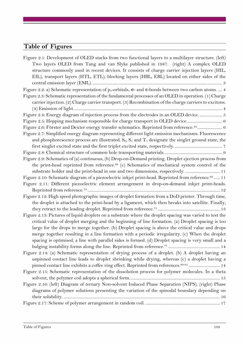
Table of Figures 109
Table of Figures
Figure 2.1: Development of OLED stacks from two functional layers to a multilayer structure. (left)
Two layers OLED from Tang and van Slyke published in 1987. (right) A complex OLED
structure commonly used in recent devices. It consists of charge carrier injection layers (HIL,
EIL), transport layers (HTL, ETL), blocking layers (HBL, EBL) located on either sides of the
central emission layer (EML). ........................................................................................................................ 3
Figure 2.2: a) Schematic representation of pz-orbitals, σ- and π-bonds between two carbon atoms. .... 4
Figure 2.3: Schematic representation of the fundamental processes of an OLED in operation. (1) Charge
carrier injection. (2) Charge carrier transport. (3) Recombination of the charge carriers to excitons.
(4) Emission of light. ......................................................................................................................................... 4
Figure 2.4: Energy diagram of injection process from the electrodes in an OLED device. ..................... 5
Figure 2.5: Hopping mechanism responsible for charge transport in OLED device. ................................ 6
Figure 2.6: Förster and Dexter energy transfer schematics. Reprinted from reference.44 ....................... 6
Figure 2.7: Simplified energy diagram representing different light emission mechanisms. Fluorescence
and phosphorescence process are illustrated. S0, S1 and T1 designate the singlet ground state, the
first singlet excited state and the first triplet excited state, respectively. ............................................ 7
Figure 2.8: Chemical structure of common hole transporting materials. ..................................................... 9
Figure 2.9: Schematics of (a) continuous, (b) Drop-on-Demand printing. Droplet ejection process from
the print-head reprinted from reference.69 (c) Schematics of mechanical system control of the
substrate holder and the print-head in one and two dimensions, respectively. ................................ 11
Figure 2.10: Schematic diagram of a piezoelectric inkjet print-head. Reprinted from reference.66 ...... 11
Figure 2.11: Different piezoelectric element arrangement in drop-on-demand inkjet print-heads.
Reprinted from reference.70 ........................................................................................................................... 12
Figure 2.12: High speed photographic images of droplet formation from a DoD printer. Through time,
the droplet is attached to the print-head by a ligament, which then breaks into satellite. Finally,
they retract to the leading droplet. Reprinted from reference.75 .......................................................... 13
Figure 2.13: Pictures of liquid droplets on a substrate where the droplet spacing was varied to test the
critical value of droplet merging and the beginning of line formation. (a) Droplet spacing is too
large for the drops to merge together. (b) Droplet spacing is above the critical value and drops
merge together resulting in a line formation with a periodic irregularity. (c) When the droplet
spacing is optimised, a line with parallel sides is formed. (d) Droplet spacing is very small and a
bulging instability forms along the line. Reprinted from reference.77 ................................................ 14
Figure 2.14: (a) Schematic representation of drying process of a droplet. (b) A droplet having an
unpinned contact line leads to droplet shrinking while drying, whereas (c) a droplet having a
pinned contact line exhibits a coffee ring effect. Reprinted from references.80-81 ............................. 14
Figure 2.15: Schematic representation of the dissolution process for polymer molecules. In a theta
solvent, the polymer coil adopts a spherical form. ................................................................................... 15
Figure 2.16: (left) Diagram of ternary Non-solvent Induced Phase Separation (NIPS). (right) Phase
diagrams of polymer solutions presenting the variation of the spinodal boundary depending on
their solubility. ................................................................................................................................................. 16
Figure 2.17: Scheme of polymer arrangement in random coil. ..................................................................... 17
110 Table of Figures
Figure 2.18: Schematic of polymer size in solution made from a good solvent (left) and from a bad
solvent (right). .................................................................................................................................................. 18
Figure 3.1: Monomer units forming the two polymers used in this work. The different monomers
drawn from (a) to (c) were present in the polymers to the proportions displayed in Table 3.1. The
dashed lines each indicate the continuation of the polymer chain. ....................................................... 21
Figure 3.2: Absorption spectra of the hole transport materials measured in spin coated films processed
from toluene. ..................................................................................................................................................... 22
Figure 3.3: Mapping of surface tension and boiling point of the investigated inkjet printing solvents.
.............................................................................................................................................................................. 24
Figure 3.4: HAAKE MARS rheometer. (a) Photo of the measurement equipment.44 (b) Diagram of
rotation cone and fixed lower plate.............................................................................................................. 26
Figure 3.5: Graphical representation of viscosity change of polymer solutions over a wide range of
shear rates. A Newtonian solution and two non-Newtonian solutions, one presenting shear
thickening and the other one shear thinning are represented. .............................................................. 26
Figure 3.6: Photograph of KRÜSS DSA 100 used for surface tension and contact angle measurement. 44 ........................................................................................................................................................................... 27
Figure 3.7: Pixdro printer LP50.44 ....................................................................................................................... 28
Figure 3.8: (a) Photograph of an inkjet printing substrate of 30 x 30 mm² containing four pixels with
an active area of 4.606 mm². (b) Microscope picture of a subpixel where a pixel contains 11 x 33
subpixels. (c) Schematic of the cross-section of a single subpixel ......................................................... 29
Figure 3.9: (a) Microscope picture of one subpixel. (b) SEM picture of bank 1 and bank 2 with one
organic layer printed in subpixel. Picture taken from the side. (c) Film profile in subpixel measured
by profilometer. The outer region of the subpixel is depicted by a red dashed box. ........................ 30
Figure 3.10: Pressure profiles with time in the vacuum chamber in dependence on the selected drying
speed. ................................................................................................................................................................... 31
Figure 3.11: Photographs of a large area film during the drying process in the vacuum chamber taken
by camera under UV illumination. An emissive material mixture was printed from menthyl
isovalerate on glass substrate and dried with the slow drying speed program. For an easier
identification at t = 0 s and t = 127 s, the substrate has been marked in grey, the wet film in white
and the dry film in orange. ............................................................................................................................. 32
Figure 3.12: Example of a measurement scan to determine layer thickness over seven subpixels of a
pixelated substrate. .......................................................................................................................................... 33
Figure 3.13: Schematic representation of a white light scanning microscopy. Reprinted from
reference.99 ......................................................................................................................................................... 34
Figure 3.14: Schematic of contact angle measurement for different inks. γVL, γVS and γLS correspond to
the surface energy at the liquid/vapor interface, at the vapour/solid interface and at the
liquid/solid interface, respectively. .............................................................................................................. 35
Figure 3.15: Contact angle-dependency on ink surface tension and substrate surface energy. ............. 35
Figure 3.16: Impact of droplet contact angle on the particle arrangement in suspension. (a) Hydrophilic
droplet leads to homogeneous repartition of the particle on the surface. (b) Hydrophobic droplet
drives the particles to aggregate in the centre. Reprinted from reference.66 ..................................... 36
Figure 3.17: Deformation of X-Po polymer surface processed from 1-methylnaphalene observed by
interferometry (left). A 90 pL drop of 3-phenoxytoluene was left on the polymer surface for five
minutes and removed by vacuum drying. Cross-section of the deformation used to quantify the
solvent exposure stability (right). ................................................................................................................ 37
Table of Figures 111
Figure 3.18: (a) Working principle of an ellipsometer. (b) Ellipsometer M-2000 from J.A. Woollam
used to measure thin film optical properties. ............................................................................................ 37
Figure 3.19: Graphical representation of the MSE depending on the layer thickness. Reproduced from
www.jawoollam.com. ...................................................................................................................................... 38
Figure 3.20: Schematic representation of a device built for electronics characterisation. Four active
areas (yellow) are formed by the overlapping anodes (light blue) and cathodes (dark blue). The
area in grey depicts the region where the printed as well as evaporated layers are deposited. .... 39
Figure 3.21: Typical space charge–limited current behaviour for polymer semiconductor. Four charge‐
transport regions are visible (i) Ohmic region (J ∝ V), (ii) trap‐SCLC region (J ∝ V1-2), (iii) TFL
region (J ∝ V2-100), and (iv) SCLC region (J ∝ V2). Reprinted from reference.104 ............................. 39
Figure 3.22: Multilayer stack of a unipolar device designed to study the mobility of the HTL. .......... 40
Figure 3.23: Bipolar device architecture employed to study the interface between the solution-
processed layers HTL and EML by varying the cross-linking degree of the HTL. ....................... 41
Figure 3.24: Chromaticity diagram displaying the CIE coordinate system. .............................................. 43
Figure 4.1: Viscosity of polymer solutions of X-Po in (a) 1-MYN, (b) 1-MXN, (c) PXT, (d) CYX and
in (e) MISO at different concentrations over a wide range of shear rates. ......................................... 45
Figure 4.2: Photographs of precipitation test. (a) Polymer solution dissolved in cyclohexyl hexanoate
at 30 g∙L-1; (b) precipitated solution after adding 21 v/v% ethanol. .................................................... 47
Figure 4.3: Experimental determination of polymer-solvent affinity. Precipitation test performed with
(a) ethanol and (b) acetone as non-solvents dropped into X-Po polymer solution from 1-MYN, 1-
MXN, PXT, CYX and in MISO. ................................................................................................................. 47
Figure 4.4: Concentration regimes for polymer solutions: dilute solution c<c*, solution at the overlap
concentration c=c*, concentrated solution c>c*...................................................................................... 48
Figure 4.5: Mark-Houwink parameter 𝛼 related to polymer organisation in solution. .......................... 49
Figure 4.6: Graphical determination of Mark-Houwink parameters 𝛼 and 𝑘 for X-Po in CYX. The
molecular weights of 81.800 g·mol-1 and 187.000 g·mol-1 were used to determine 𝛼 and 𝑘. ........ 50
Figure 4.7: Graphical determination of the intrinsic viscosity [η] of X-Po in CYX. The molecular
weights of 81.800 g·mol-1 and 187.000 g·mol-1 were used to determine [η]. ................................... 50
Figure 4.8: Spread of 𝛼 value calculated from the uncertainties in the polydispersity and in the
measurement errors. ....................................................................................................................................... 51
Figure 4.9: Graphical determination of the Huggins constant KH (left) and Kramer constant KK (right)
for the polymer solution of X-Po in CYX. The molecular weight of 81.800 g·mol-1 was used for
the determination of KH and KK. The y-intercept of the Huggins and Kramer plots is the intrinsic
viscosity of the polymer solution. ................................................................................................................ 52
Figure 4.10: Determination of intrinsic viscosity by Huggins and Kramer equations of X-Po solutions
from (a) 1-MYN, (b) 1-MXN, (c) PXT, (d) CYX and (e) MISO. The intrinsic viscosity is the
viscosity of the polymer solution at concentration zero. ........................................................................ 53
Figure 4.11: Radius of gyration 𝑅𝑔 of a random coil polymer in solution. ................................................ 55
Figure 4.12: Volume fraction 𝛷 of X-Po in the five solvents for various concentrations. ...................... 57
Figure 4.13: Size distribution of X-Po in all solvents represented by (a) intensity and (b) volume. .... 58
Figure 5.1: Resulting species of the cross-linking reaction of two styrene units, disclosed by US patent
from reference.126 ............................................................................................................................................. 61
Figure 5.2: Infrared spectra of polymer powders of 7X-Po and X-Po before and after cross-linking
through one DSC run from room temperature to 300°C at 20 K·min-1. The spectrum of 7X-Po is
112 Table of Figures
displayed in (a) from 850 cm-1 to 1200 cm-1 and in (b) from 1530 cm-1 to 1665 cm-1. The spectrum
of X-Po is displayed in (c) from 850 cm-1 to 1200 cm-1 and in (d) from 1530 cm-1 to 1665 cm-1... 62
Figure 5.3: Thermograms of (a) Po and (b) X-Po polymer powders. The thermograms were recorded
with a single heat ramp from room temperature to 300°C at a heating rate of 20 K∙min-1. .......... 64
Figure 5.4: Thermal analysis of X-Po from room temperature to 500°C measured by TGA in nitrogen
atmosphere. ........................................................................................................................................................ 64
Figure 5.5: DSC thermogram of polymer X-Po powder in a heat-cool-heat cycle between room
temperature and 300°C at a heating rate of 20 K∙min-1. ......................................................................... 64
Figure 5.6: X-Po powder after undergoing a DSC run in a crucible from room temperature to 300°C
(left) and after being stirred in 3-phenoxytoluene at a nominal concentration of 5 g∙L-1 for 24 hours
(right). 0% ±1% weight loss of the sample was measured after removing the supernatant of solvent
and drying the solid. ........................................................................................................................................ 65
Figure 5.7: Viscosities polymer solutions of 50 g∙L-1.measured at room temperature after heat
treatment for three hours at indicated temperature. The viscosities are normalised to the solution
viscosity before heat treatment. .................................................................................................................... 66
Figure 5.8: Intensity size distribution of X-Po in (a) 1-methylnaphthalene, (b) 1-methoxynaphthalene,
(c) 3-phenoxytoluene, (d) cyclohexyl hexanoate, (e) menthyl isovalerate at a concentration of 50
g∙L-1 measured by DLS after exposure to 140°C and/or 160°C and/or 180°C and/or 200°C. All
polymer solutions after heat treatment are measured at 25°C. ............................................................. 68
Figure 5.9: Volume size distribution of X-Po in (a) 1-methylnaphthalene, (b) 1-methoxynaphthalene,
(c) 3-phenoxytoluene, (d) cyclohexyl hexanoate, (e) menthyl isovalerate at a concentration of 50
g∙L-1 measured by DLS. The polymer solutions were exposed to different temperature treatments,
then cooled down and measured at 25°C. ................................................................................................... 69
Figure 5.10: Thermograms of (a) X-Po in 3-phenoxytoluene at 50 g∙L-1 without vacuum drying
measured with 30 K∙min-1 heating rate, (b) X-Po in 3-phenoxytoluene at 50 g∙L-1 after 30 minutes
of vacuum drying measured with 20 K∙min-1 heating rate, (c) X-Po in toluene at 50 g∙L-1 after 30
minutes of vacuum drying measured with 20 K∙min-1 heating rate. .................................................... 70
Figure 5.11: Ink wetting on glass substrate of X-Po inks from cyclohexyl hexanoate and from menthyl
isovalerate at 5g·L-1. (left) Picture of X-Po ink droplet dropped taken from the side, used to
determine the surface tension of the ink. The baseline is blue; the drop outline is green and the
tangent is red. (right) Picture of X-Po printed ink droplets taken from the fiducial camera of the
printer. Different amounts of ink were printed. Four series were printed (from top to bottom): 30
pL, 10 pL, 20 pL and 20 pL............................................................................................................................ 72
Figure 5.12: Schematic representation of ink wetting and drops merging resulting in wet film
formation through ink levelling. .................................................................................................................. 72
Figure 5.13: Interferometry picture and cross-section of a printed film demonstrating the coffee-ring
effect. (a) 3D picture of the film corner where the coffee-ring effect is visible. (b) Cross-section of
the same film, where the coffee-ring effect is identified by a blue circle. ............................................ 73
Figure 5.14: Thin film images taken by interferometry. X-Po films processed from MISO suffering of
formation instabilities such as Marangoni and coffee-ring effect. The droplet spacing is (a) 30µm,
(b) 35 µm, (c) 22 µm and (d) 20 µm in both x and y direction................................................................ 73
Figure 5.15: Trapped solvent in X-Po films after two hours vacuum drying determined by mass loss.
.............................................................................................................................................................................. 74
Figure 5.16: Newly developed measurement procedure to determine the solvent residue in X-Po film
after the annealing step. .................................................................................................................................. 75

Table of Figures 113
Figure 5.17: Surface deformation of X-Po film processed from 1-methylnaphalene caused by a 90 pL
drop of 3-phenoxytoluene left on the film surface for five minutes and removed by vacuum drying.
(left) Surface deformation observed by interferometry and represented as 3D picture. (right)
Example of the cross-section of a typical surface deformation used to quantify the film stability
against solvent exposure. ............................................................................................................................... 76
Figure 5.18: Deformation heights caused by 3-phenoxytoluene drop exposure on IJP polymer X-Po
thin films depending on the ink solvent. The polymer films were 70 nm thick and were processed
from 1-MYN, 1-MXN, PXT, CYX and MISO. ....................................................................................... 77
Figure 5.19: 3D pictures of the deformation visible on X-Po thin films processed from 1-MYN, 1-
MXN, PXT, CYX and MISO caused by 3-phenoxytoluene drop exposure. The pictures were taken
by interferometry. The polymer films were 70 nm thick. ...................................................................... 77
Figure 5.20: X-Po films deformation caused by 3-phenoxytoluene drop exposure on polymer films of
various thicknesses. ......................................................................................................................................... 78
Figure 5.21: 3D pictures of the deformation visible on X-Po thin film processed from 1-MXN caused
by PXT exposure. The pictures were taken by interferometry. The film deformation depends on
the layer thickness. .......................................................................................................................................... 78
Figure 5.22: Film deformation following exposure to 3-phenoxytoluene on the 70 nm thick polymer
films after annealing at different temperatures. ........................................................................................ 79
Figure 5.23: 3D pictures of the deformation visible on X-Po thin films processed from 1-MYN, 1-
MXN, PXT, CYX and MISO and annealed at 225°C and 250°C, respectively, caused by PXT
exposure. The pictures were taken by interferometry. The polymer films are 70 nm thick. ........ 79
Figure 5.24: Cross-linking thermograms of X-Po in films measured by DSC from room temperature
to 300°C. The area below the curve identified by the grey hatching was used to determine the
cross-linking reaction enthalpy. An offset was applied to all thermograms for the sake of visibility.
For the y-axis, each graduation corresponds to 0.2 W∙g-1. .................................................................... 80
Figure 5.25: Mean square error calculated for X-Po thin films’ absorption over wavelength range from
250 to 1000 nm. The thin films were processed from 1-MYN, PXT and MISO and were annealed
either at 160°C, 200°C or 225°C. ................................................................................................................. 82
Figure 5.26: Impact of processing ink solvent affinity with X-Po on the cross-linking degree in film
and on the calculated MSE value measured by ellipsometry. The MSE value characterises the
difference between the model, describing a X-Po cross-linked spin-coated film, and the measured
data for the Ψ and Δ values of X-Po inkjet printing films. .................................................................... 83
Figure 6.1: Electroluminescent pictures of OLED device subpixels taken at a luminescence of 1000
cd∙m-2. The HTL polymer was processed from PXT, CYX and MISO. On each HTL, an EML was
processed from PXT, CYX and MISO. ...................................................................................................... 87
Figure 6.2: Photograph of contact angle measurement. ................................................................................. 88
Figure 6.3: Pictures of 90 pL drop of 3-phenoxytoluene dropped onto X-Po films processed from 1-
MYN, 1-MXN, PXT, CYX and from MISO. Pictures were taken by the printer camera. ........... 89
Figure 6.4: Schematic of the profilometer needle scanning a substrate exhibiting a substantial height
change that can be assimilated to the subpixel banks. The needle is drawn at various times of a
scan. ..................................................................................................................................................................... 90
Figure 6.5: HIL, HTL and EML layers profiles measured by profilometer in a subpixel. The HIL is
common to all subpixels. The HTL was printed from (a) 1-MYN, (b) 1-MXN, (c) PXT, (d) CYX
and (e) MISO. The EML was processed from PXT in all subpixels. The active area of a subpixel
114 Table of Figures
is depicted by a blue arrow in (a). The HIL, the HTL and the EML were printed to reach 40 nm,
20 nm and 80 nm, respectively, in the centre of the subpixels. ............................................................. 90
Figure 6.6: Comparison of EML profiles obtained by printing inks from PXT and MISO onto X-Po
from PXT. The profiles were measured in a subpixel by profilometry. ............................................. 91
Figure 6.7: Current density vs voltage characteristics of HODs. The devices were built from 40 nm
HIL films / HTL of 35 nm X-Po films from 1-MXN. The curves of the pixels (A in purple, B in
red, C in cyan) and the linear fitting of n=1 are plotted on double logarithmic scales. .................. 92
Figure 6.8: Bipolar OLED devices performance with EML processed from PXT. Object of the study is
the HTL annealing temperature. (a) J-V characteristics of OLED devices as a function of the HTL
annealing temperature. (b) Efficiencies of OLED devices with HTL annealed at various
temperatures. (c) Luminance lifetimes of OLED devices with HTL annealed at various
temperatures. ..................................................................................................................................................... 93
Figure 6.9: Bipolar OLED device performance with the EML processed from PXT. Object of the study
is the impact of the HTL ink solvent in case of an HTL annealing temperature of 225°C. (a)
Efficiency of OLED devices with the HTL processed from various solvents. (b) Luminance lifetime
of OLED devices with the HTL processed from various solvents. ...................................................... 95
Figure 6.10: OLED performance in case of the EML being processed from PXT. Object of the study is
to understand the impact of the HTL ink solvent when the HTL is annealed at 180°C. (a) Efficiency
and (b) lifetimes of OLEDs in dependence of the HTL processing solvent as indicated. ............... 96
Figure 6.11: Performance of OLEDs where the EML was processed from MISO. Object of the study
is the impact of the HTL ink solvent at an HTL annealing temperature of 180°C. (a) Efficiency of
OLED devices with the HTL processed from various solvents. (b) Luminance lifetime of OLED
devices with the HTL processed from various solvents. ........................................................................ 97
Figure 6.12: Electroluminescence photos of OLED devices taken by a microscope camera of single
subpixels. The HTL of these devices was processed from (a) 1-MYN, (b) PXT, (c) CYX and (d)
MISO. Pictures were taken at device luminance of 1000 cd∙m-2. White frames were added to better
recognise the emissive areas of the four subpixels. .................................................................................. 97
Figure 6.13: Impact of EML ink solvent on OLED performance in case of the HTL processed from
PXT and annealed at either 180°C or 225°C. ........................................................................................... 98

Table of Tables 115
Table of Tables
Table 3.1: Monomer units contained in X-Po and Po. .................................................................................... 22
Table 3.2: HOMO and LUMO levels of X-Po and Po. HOMO values of the hole transport materials
measured by photoelectron spectroscopy (Riken) and the calculated LUMO of these materials. 22
Table 3.3: Inkjet printing solvents used in this work to process the hole transport material. .............. 23
Table 4.1: Determination of the overlap concentration c*, determining the upper limit of the dilute
regime of X-Po polymer solution from different solvents. .................................................................... 49
Table 4.2: Mark-Houwink parameters and intrinsic viscosities of X-Po solutions from 1-MYN, 1-
MXN, PXT, CYX and in MISO. ................................................................................................................. 51
Table 4.3: Huggins and Kramer constants KH and KK, respectively. ........................................................... 52
Table 4.4: Intrinsic viscosities determined from Mark-Houwink equation, Huggins equation, Kramer
equation and Solomon Ciuta equation. ....................................................................................................... 54
Table 4.5: Radius of gyration of X-Po in the different solvents calculated by Flory and Fox equation.
.............................................................................................................................................................................. 56
Table 5.1: Photographs of X-Po solutions from cyclohexyl hexanoate and from menthyl isovalerate
after a heat treatment of 170°C and 180°C for three hours and cooling down to room temperature.
.............................................................................................................................................................................. 66
Table 5.2: Temperatures applied to the polymer solutions for 3 hours prior to DLS measurements
which were performed at room temperature. The purpose was to identify the progress of cross-
linking in solution. ........................................................................................................................................... 67
Table 5.3: Comparison of cross-linking enthalpies and peaks of reaction of X-Po polymer powder and
of X-Po films obtained from the five IJP solvent solutions after two hours vacuum drying,
measured by DSC from room temperature to 300°C. The X-Po powder is used without solvent.
.............................................................................................................................................................................. 81
Table 6.1: Contact angle of PXT dropped on X-Po films processed from 1-MYN, 1-MXN, PXT, CYX
and MISO. The results have an uncertainty of ±5° which was determined by multiple contact angle
measurements of PXT on X-Po layers processed from MISO. The displayed value of PXT contact
angle on X-Po layer processed from MISO is an averaged value over 6 measurements................ 88


List of Abbreviations 117
List of Abbreviations
ATR Attenuated Total Reflectance
CCD Charge-Coupled Device
DIPS Diffusion Induced Phase Separation
DLS Dyanimic Light Scattering
DoD Drop on Demand
DOS Density of State
EBL Electron Blocking Layer
EIL Electron Injection Layer
EL Electroluminescence
EML Emissive Layer
EQE External Quantum Efficiency
ETL Electron Transport Layer
FTIR Fourier-Transform Infrared Spectroscopy
GPC Gel Permeation Chromatography
HBL Hole Blocking Layer
HIL Hole Injection Layer
HOD Hole Only Device
HOMO Highest Occupied Molecular Orbital
HTL Hole Transport Layer
HTM Hole Transport Material
IR Infrared
ITO Indium Tin Oxide
LCD Liquid Crystal Display
LED Light Emitting Diode
LT Lifetime
LUMO Lowest Unoccupied Molecular Orbital
MSE Mean-Square-Error
NIPS Non-solvent Induced Phase Separation
PPI Pixel Per Inch
PCS Photon Correlation Spectroscopy
OFET Organic Field-Effect Transistor
OLED Organic Light Emitting Diode

118 List of Abbreviations
OPV Organic Photovoltaic
QELS Quasi-Elastic Light Scattering
SCLC Space Charge Limited Current
SFT Surface Tension
TAA Triaryl Amine
TGA Thermal Gravimetry Analysis
PVD Physical Vapour Deposition

Formula Directory 119
Formula Directory
𝛼 and 𝑘 Mark-Houwink parameters
�̇� shear rate 1/s
𝛾𝑒−ℎ charge carrier balance between injected holes and electrons in the EML (should be 1)
ε dielectric constant
ε0 vacuum permittivity
𝜂 viscosity of the suspension mPa∙s
[𝜂] intrinsic viscosity of the polymer in the specific solvent
𝜂𝑒𝑥𝑡 external quantum efficiency
𝜂𝑓 ratio of radiative transition from singlet excitons.
𝜂𝐿 luminous efficiency in the unit cd·A-1
𝜂𝑟 relative viscosity
𝜂𝑠 viscosity of the medium
𝜂𝑠𝑝 specific viscosity
µ charge mobility
π bonding molecular orbital
π* anti-bonding molecular orbital
σ shear stress in mPa
𝛷 volume fraction of solids in the suspension
𝛷′ a universal constant independent of temperature and polymer-solvent system where 𝛷′= 2.1
x 1026 kmol-1
𝜑𝑜𝑝𝑡 outcoupling efficiency: ratio of light emitted at the surface to the light produced in the bulk
of the device (estimated 20%)
𝜒𝑠/𝑡 fraction of generated excitons which can decay radiatively (0.25 in fluorescence, 1 in
phosphorescence)
𝜔 angular speed
A active luminous area A= 4.606 mm²
c concentration of polymer
c* overlap concentration
D diffusion coefficient
dH hydrodynamic diameter

120 Formula Directory
DS droplet spacing
e elementary electron charge 1.6021765×10⁻¹⁹ C
Eb Injection barrier
EF Fermi level
Eg energy gap
f printing frequency
ΔH(Sx) cross-linking enthalpy of the polymer in film
ΔH(S0) cross-linking enthalpy in powder without solvent
I current in mA
j current density in mA·cm-²
k extinction coefficient
kB Boltzmann constant 1.38 × 10⁻²³ m2∙kg∙s-2∙K-1
KH Huggins constant
KK Kramer constant
𝐿 luminance in cd·m²
𝐿0 initial luminance
mf total mass after drying of material and solvent residue
ms mass of solvent residue in bulk
𝑀𝑤 molecular weight
n index of refraction
𝐴𝐹 the acceleration factor must be determined for each colour
𝑞 sample heat flow
𝑅 resistance of a thermocouple
rc effective interactive capture radius
𝑅𝑔 radius of gyration
Rh hydrodynamic radius
rs solvent residue in w%
S0 singlet ground state
S1 first singlet excited state
T temperature
𝑇𝑔 transition glass
∆𝑇 temperature difference between the sample pan and the reference pan
V0 applied voltage
vprint printing speed

Formula Directory 121
𝑋(𝑆𝑥) cross linking degree

List of References 123
List of References
1. Inoguchi, T.; Takeda, M.; Kakihara, Y.; Nakata, Y.; Yoshida, M., Stable High-Brightness Thin-Film Electroluminescent Panels. J. SID 1974 digest International Symposium 1974, 84.
2. Tang, C. W.; VanSlyke, S. A., Organic Electroluminescent Diodes. Appl. Phys. Lett. 1987, 51, 913-915. 3. Shirakawa, H.; Louis, E. J.; MacDiarmid, A. G.; Chiang, C. K.; Heeger, A. J., Synthesis of Electrically
Conducting Organic Polymers: Halogen Derivatives of Polyacetylene,(Ch)X. J. Chem. Soc. Chem. Comm. 1977, 578-580.
4. Burroughes, J. H.; Bradley, D. D.; Brown, A.; Marks, R.; Mackay, K.; Friend, R. H.; Burns, P.; Holmes, A., Light-Emitting Diodes Based on Conjugated Polymers. Nature 1990, 347, 539.
5. Gustafsson, G.; Cao, Y.; Treacy, G.; Klavetter, F.; Colaneri, N.; Heeger, A., Flexible Light-Emitting Diodes Made from Soluble Conducting Polymers. Nature 1992, 357, 477.
6. Ishii, H.; Sugiyama, K.; Ito, E.; Seki, K., Energy Level Alignment and Interfacial Electronic Structures at Organic/Metal and Organic/Organic Interfaces. Adv. Mater. 1999, 11, 605-625.
7. Parker, I. D., Carrier Tunneling and Device Characteristics in Polymer Light‐Emitting Diodes. J. Appl. Phys. 1994, 75, 1656-1666.
8. Su, W.-F.; Chen, Y., Synthesis and Optoelectronic Properties of Thermally Cross-Linkable Hole-Transporting Poly (Fluorene-Co-Triphenylamine). Polymer 2011, 52, 77-85.
9. Li, Y.-J.; Sasabe, H.; Su, S.-J.; Tanaka, D.; Takeda, T.; Pu, Y.-J.; Kido, J., Highly Efficient Green Phosphorescent Oled Based on Pyridine-Containing Starburst Electron-Transporting Materials. Chem. Lett. 2010, 39, 140-141.
10. Søndergaard, R. R.; Hösel, M.; Krebs, F. C., Roll‐to‐Roll Fabrication of Large Area Functional Organic Materials. J. Polym. Sci., Part B: Polym. Phys. 2013, 51, 16-34.
11. Bharathan, J.; Yang, Y., Polymer Electroluminescent Devices Processed by Inkjet Printing: I. Polymer Light-Emitting Logo. Appl. Phys. Lett. 1998, 72, 2660-2662.
12. Zhong, C.; Duan, C.; Huang, F.; Wu, H.; Cao, Y., Materials and Devices toward Fully Solution Processable Organic Light-Emitting Diodes. Chem. Mater. 2010, 23, 326-340.
13. Li, Y., Rgb Printed Amoled: Challenges and Opportunities. SID Symposium Digest of Technical Papers 2018, 49, 95-98.
14. Shao, L.-Q.; Ting-Dong; Liang, J.-S.; Bi, Z.-T.; Zhe-Li; Jingyao-Song; Huo, S.-T., The Development of 403 Ppi Real Rgb Printing Amoled. SID Symposium Digest of Technical Papers 2019, 50, 1943-1945.
15. Prakash, S.; Sims, M.; Wyrsta, I.; Parker, I. D.; Kondakov, D.; Gao, W., Solution-Processed Oleds: Unique Challenges and Advantages. SID Symposium Digest of Technical Papers 2013, 44, 678-681.
16. Ho, S.; Chen, Y.; Liu, S.; Peng, C.; Zhao, D.; So, F., Interface Effect on Efficiency Loss in Organic Light Emitting Diodes with Solution Processed Emitting Layers. Adv. Mater. Interfaces 2016, 3, 1600320.
17. Smith, A. R.; Lee, K. H.; Nelson, A.; James, M.; Burn, P. L.; Gentle, I. R., Diffusion–the Hidden Menace in Organic Optoelectronic Devices. Adv. Mater. 2012, 24, 822-826.
18. Steuerman, D. W.; Garcia, A.; Dante, M.; Yang, R.; Löfvander, J. P.; Nguyen, T. Q., Imaging the Interfaces of Conjugated Polymer Optoelectronic Devices. Adv. Mater. 2008, 20, 528-534.
19. Perumal, A.; Faber, H.; Yaacobi‐Gross, N.; Pattanasattayavong, P.; Burgess, C.; Jha, S.; McLachlan, M.
A.; Stavrinou, P. N.; Anthopoulos, T. D.; Bradley, D. D., High‐Efficiency, Solution‐Processed, Multilayer
Phosphorescent Organic Light‐Emitting Diodes with a Copper Thiocyanate Hole‐Injection/Hole‐Transport Layer. Adv. Mater. 2015, 27, 93-100.
20. Huang, F.; Cheng, Y.-J.; Zhang, Y.; Liu, M. S.; Jen, A. K. Y., Crosslinkable Hole-Transporting Materials for Solution Processed Polymer Light-Emitting Diodes. J. Mater. Chem. 2008, 18, 4495-4509.
21. Huang, F.; Wu, H.; Cao, Y., Water/Alcohol Soluble Conjugated Polymers as Highly Efficient Electron Transporting/Injection Layer in Optoelectronic Devices. Chem. Soc. Rev. 2010, 39, 2500-2521.
22. Sax, S.; Rugen‐Penkalla, N.; Neuhold, A.; Schuh, S.; Zojer, E.; List, E. J.; Müllen, K., Efficient Blue‐Light‐Emitting Polymer Heterostructure Devices: The Fabrication of Multilayer Structures from Orthogonal Solvents. Adv. Mater. 2010, 22, 2087-2091.
23. Cheng, Y.-J.; Liu, M. S.; Zhang, Y.; Niu, Y.; Huang, F.; Ka, J.-W.; Yip, H.-L.; Tian, Y.; Jen, A. K. Y., Thermally Cross-Linkable Hole-Transporting Materials on Conducting Polymer: Synthesis,
124 List of References
Characterization, and Applications for Polymer Light-Emitting Devices. Chem. Mater. 2008, 20, 413-422.
24. Müller, C. D.; Falcou, A.; Reckefuss, N.; Rojahn, M.; Wiederhirn, V.; Rudati, P.; Frohne, H.; Nuyken, O.; Becker, H.; Meerholz, K., Multi-Colour Organic Light-Emitting Displays by Solution Processing. Nature 2003, 421, 829.
25. Li, W., et al., Covalently Interlinked Organic Led Transport Layers Via Spin-Coating/Siloxane Condensation. Adv. Mater. 1999, 11, 730-734.
26. Tseng, S.-R.; Lin, S.-C.; Meng, H.-F.; Liao, H.-H.; Yeh, C.-H.; Lai, H.-C.; Horng, S.-F.; Hsu, C.-S., General Method to Solution-Process Multilayer Polymer Light-Emitting Diodes. Appl. Phys. Lett. 2006, 88, 163501.
27. Chen, C.-Y., et al., Continuous Blade Coating for Multi-Layer Large-Area Organic Light-Emitting Diode and Solar Cell. J. Appl. Phys. 2011, 110, 094501.
28. Yeh, H.-C.; Meng, H.-F.; Lin, H.-W.; Chao, T.-C.; Tseng, M.-R.; Zan, H.-W., All-Small-Molecule Efficient White Organic Light-Emitting Diodes by Multi-Layer Blade Coating. Org. Electron. 2012, 13, 914-918.
29. Garcia, A.; Yang, R.; Jin, Y.; Walker, B.; Nguyen, T.-Q., Structure-Function Relationships of Conjugated Polyelectrolyte Electron Injection Layers in Polymer Light Emitting Diodes. Appl. Phys. Lett. 2007, 91, 153502.
30. Ma, W.; Iyer, P. K.; Gong, X.; Liu, B.; Moses, D.; Bazan, G. C.; Heeger, A. J., Water/Methanol‐Soluble
Conjugated Copolymer as an Electron‐Transport Layer in Polymer Light‐Emitting Diodes. Adv. Mater. 2005, 17, 274-277.
31. Zhang, Y.; Huang, F.; Chi, Y.; Jen, A. K. Y., Highly Efficient White Polymer Light‐Emitting Diodes
Based on Nanometer‐Scale Control of the Electron Injection Layer Morphology through Solvent Processing. Adv. Mater. 2008, 20, 1565-1570.
32. Hansen, E. F.; Derrick, M. R.; Schilling, M. R.; Garcia, R., The Effects of Solution Application on Some Mechanical and Physical Properties of Thermoplastic Amorphous Polymers Used in Conservation: Poly(Vinyl Acetate)S. J. Am. Inst. Conserv. 1991, 30, 203-213.
33. Olayemi, J. Y.; Adeyeye, A. A., Some Properties of Polyvinyl Acetate Films Cast from Methanol, Acetone and Chloroform as Solvent. Polym. Test. 1982, 3, 25-35.
34. Ohisa, S.; Matsuba, G.; Yamada, N. L.; Pu, Y.-J.; Sasabe, H.; Kido, J., Precise Evaluation of Angstrom-Ordered Mixed Interfaces in Solution-Processed Oleds by Neutron Reflectometry. Adv. Mater. 2014, 1, 1400097.
35. Kang, P.-G.; Shin, D. H.; Na, H.-Y.; Doh, Y.-J.; John, K.; Liam, S.; Suh, M. C., The Interfacial Effect between Htl and Eml on the Efficiency of Solution Processed Green Phosphorescent Oleds. SID Symposium Digest of Technical Papers 2016, 47, 494-497.
36. Pope, M.; Kallmann, H.; Magnante, P., Electroluminescence in Organic Crystals. J. Chem. Phys. 1963, 38, 2042-2043.
37. Helfrich, W.; Schneider, W., Recombination Radiation in Anthracene Crystals. Phys. Rev. Lett. 1965, 14, 229.
38. Geffroy, B.; Le Roy, P.; Prat, C., Organic Light‐Emitting Diode (Oled) Technology: Materials, Devices and Display Technologies. Polym. Int. 2006, 55, 572-582.
39. Gaspar, D. J.; Polikarpov, E., Oled Fundamentals: Materials, Devices, and Processing of Organic Light-Emitting Diodes; CRC press, 2015.
40. Bässler, H., Charge Transport in Disordered Organic Photoconductors a Monte Carlo Simulation Study. Phys. Status Solidi B 1993, 175, 15-56.
41. Heun, S.; Bässler, H.; Borsenberger, P., The Spectral Assessment of the Origin of the Polaronic Contribution to Charge Transport in a Highly Conjugated Triarylamine Donor Molecule. Chem. Phys. 1995, 200, 265-270.
42. Brütting, W., Physics of Organic Semiconductors. Phys. Status Solidi A 2004, 201, 1031-1031. 43. Van der Holst, J.; Van Oost, F.; Coehoorn, R.; Bobbert, P., Electron-Hole Recombination in Disordered
Organic Semiconductors: Validity of the Langevin Formula. Phys. Rev. B 2009, 80, 235202. 44. https://www.thermofisher.com/order/catalog/product/379-0340 (accessed 28.10.2019). 45. Baldo, M.; O’brien, D.; Thompson, M.; Forrest, S., Excitonic Singlet-Triplet Ratio in a Semiconducting
Organic Thin Film. Phys. Rev. B 1999, 60, 14422.
List of References 125
46. Baldo, M. A.; O'brien, D.; You, Y.; Shoustikov, A.; Sibley, S.; Thompson, M.; Forrest, S. R., Highly Efficient Phosphorescent Emission from Organic Electroluminescent Devices. Nature 1998, 395, 151-154.
47. Salaneck, W. R.; Lundström, I.; Rånby, B. G., Conjugated Polymers and Related Materials: The Interconnection of Chemical and Electronic Structure: Proceedings of the Eighty-First Nobel Symposium; Oxford University Press, USA, 1993; Vol. 81.
48. Taylor, D., Vacuum-Thermal-Evaporation: The Route for Roll-to-Roll Production of Large-Area Organic Electronic Circuits. Semicond. Sci. Technol. 2015, 30, 054002.
49. Newby, C.; Lee, J.-K.; Ober, C. K., The Solvent Problem: Redissolution of Macromolecules in Solution-Processed Organic Electronics. Macromol. Res. 2013, 21, 248-256.
50. Trattnig, R.; Pevzner, L.; Jäger, M.; Schlesinger, R.; Nardi, M. V.; Ligorio, G.; Christodoulou, C.; Koch,
N.; Baumgarten, M.; Müllen, K., Bright Blue Solution Processed Triple‐Layer Polymer Light‐Emitting Diodes Realized by Thermal Layer Stabilization and Orthogonal Solvents. Adv. Funct. Mater. 2013, 23, 4897-4905.
51. Böhm, E.; Levermore, P.; Tseng, H.-R.; Bealle, G.; Wang, H.-J.; Hibon, P.; Heil, H.; Jatsch, A.; Buchholz, H., Ink-Jet-Printed Oled Displays. 2017.
52. Zhu, M.; Yang, C., Blue Fluorescent Emitters: Design Tactics and Applications in Organic Light-Emitting Diodes. Chem. Soc. Rev. 2013, 42, 4963-4976.
53. Zhang, Z.; Wang, Q.; Dai, Y.; Liu, Y.; Wang, L.; Ma, D., High Efficiency Fluorescent White Organic Light-Emitting Diodes with Red, Green and Blue Separately Monochromatic Emission Layers. Org. Electron. 2009, 10, 491-495.
54. Lou, Y.; Okawa, Y.; Wang, Z.; Naka, S.; Okada, H., Efficient Electron Transport in 4, 4′-Bis [N-(1-Napthyl)-N-Phenyl-Amino] Biphenyl and the Applications in White Organic Light Emitting Devices. Org. Electron. 2013, 14, 1015-1020.
55. Shirakawa, H., Nobel Lecture: The Discovery of Polyacetylene Film—the Dawning of an Era of Conducting Polymers. Rev. Mod. Phys. 2001, 73, 713.
56. Shahnawaz; Sudheendran Swayamprabha, S.; Nagar, M. R.; Yadav, R. A. K.; Gull, S.; Dubey, D. K.; Jou, J.-H., Hole-Transporting Materials for Organic Light-Emitting Diodes: An Overview. J. Mater. Chem. C 2019, 7, 7144-7158.
57. Schols, S.; Verlaak, S.; Rolin, C.; Cheyns, D.; Genoe, J.; Heremans, P., An Organic Light‐Emitting Diode
with Field‐Effect Electron Transport. Adv. Funct. Mater. 2008, 18, 136-144. 58. Benvenho, A. R. V.; Serbena, J. P. M.; Lessmann, R.; Hümmelgen, I. A.; Mello, R. M. Q. d.; Li, R. W. C.;
Cuvero, J. H.; Gruber, J., Efficient Organic Light-Emitting Diodes with Fluorine-Doped Tin-Oxide Anode and Electrochemically Synthesized Sulfonated Polyaniline as Hole Transport Layer. Braz. J. Phys. 2005, 35, 1016-1019.
59. Park, S.-R.; Kang, J.-H.; Ahn, D. A.; Suh, M. C., A Cross-Linkable Hole Transport Material Having Improved Mobility through a Semi-Interpenetrating Polymer Network Approach for Solution-Processed Green Pholeds. J. Mater. Chem. C 2018, 6, 7750-7758.
60. Grigalevicius, S.; Zhang, B.; Xie, Z.; Forster, M.; Scherf, U., Polycarbazole-Based Networks Made by Photo-Crosslinking for Hole Transporting Layers of Oled Devices. Org. Electron. 2011, 12, 2253-2257.
61. Zuniga, C. A.; Barlow, S.; Marder, S. R., Approaches to Solution-Processed Multilayer Organic Light-Emitting Diodes Based on Cross-Linking. Chem. Mater. 2011, 23, 658-681.
62. Günes, S.; Neugebauer, H.; Sariciftci, N. S., Conjugated Polymer-Based Organic Solar Cells. Chem. Rev. 2007, 107, 1324-1338.
63. Kawase, T.; Shimoda, T.; Newsome, C.; Sirringhaus, H.; Friend, R. H., Inkjet Printing of Polymer Thin Film Transistors. Thin solid films 2003, 438, 279-287.
64. Jeanmaire, D. L.; Hawkins, G. A.; Sharma, R. Continuous Inkjet Printhead with Selectable Printing Volumes of Ink. 2003.
65. Bogy, D. B.; Talke, F. E., Experimental and Theoretical Study of Wave Propagation Phenomena in Drop-on-Demand Ink Jet Devices. IBM J. Res. Dev. 1984, 28, 314-321.
66. Tekin, E.; Smith, P. J.; Schubert, U. S., Inkjet Printing as a Deposition and Patterning Tool for Polymers and Inorganic Particles. Soft Matter. 2008, 4, 703-713.
67. Lee, E. R., Microdrop Generation; CRC press, 2018. 68. Sirringhaus, H.; Sele, C. W.; Werte, v., T.; Ramsdale, C., Organic Electronics: Materials, Manufacturing, and
Applications; John Wiley & Sons, 2006. 69. http://fab.cba.mit.edu/classes/865.18/additive/inkjet-printing/index.html (accessed 28.10.2019).
126 List of References
70. Brünahl, J.; Grishin, A. M., Piezoelectric Shear Mode Drop-on-Demand Inkjet Actuator. Sensor. Actuat A-Phys 2002, 101, 371-382.
71. Smith, P. J.; Morrin, A., An Introduction. In Reactive Inkjet Printing, 2017; pp 1-11. 72. Fromm, J. E., Numerical Calculation of the Fluid Dynamics of Drop-on-Demand Jets. IBM J. Res. Dev.
1984, 28, 322-333. 73. Singh, M.; Haverinen, H. M.; Dhagat, P.; Jabbour, G. E., Inkjet Printing - Process and Its Applications.
Adv. Mater. 2010, 22, 673-685.
74. de Gans, B.; Kazancioglu, E.; Meyer, W.; Schubert, U. S., Ink‐Jet Printing Polymers and Polymer Libraries Using Micropipettes. Macromol. Rapid Commun. 2004, 25, 292-296.
75. Jang, D.; Kim, D.; Moon, J., Influence of Fluid Physical Properties on Ink-Jet Printability. Langmuir 2009, 25, 2629-2635.
76. Tekin, E.; Holder, E.; Kozodaev, D.; Schubert, U. S., Controlled Pattern Formation of Poly[2-Methoxy-
5-(2′-Ethylhexyloxyl)–1,4-Phenylenevinylene] (Meh–Ppv) by Ink-Jet Printing. Adv. Funct. Mater. 2007, 17, 277-284.
77. Soltman, D.; Subramanian, V., Inkjet-Printed Line Morphologies and Temperature Control of the Coffee Ring Effect. Langmuir 2008, 24, 2224-2231.
78. Tekin, E.; de Gans, B.-J.; Schubert, U. S., Ink-Jet Printing of Polymers – from Single Dots to Thin Film Libraries. J. Mater. Chem. 2004, 14, 2627-2632.
79. Tekoglu, S.; Hernandez-Sosa, G.; Kluge, E.; Lemmer, U.; Mechau, N., Gravure Printed Flexible Small-Molecule Organic Light Emitting Diodes. Org. Electron. 2013, 14, 3493-3499.
80. Deegan, R. D., Pattern Formation in Drying Drops. Phys. Rev. E 2000, 61, 475-485. 81. Deegan, R. D.; Bakajin, O.; Dupont, T. F.; Huber, G.; Nagel, S. R.; Witten, T. A., Capillary Flow as the
Cause of Ring Stains from Dried Liquid Drops. Nature 1997, 389, 827-829. 82. Ko, H.-Y.; Park, J.; Shin, H.; Moon, J., Rapid Self-Assembly of Monodisperse Colloidal Spheres in an Ink-
Jet Printed Droplet. Chem. Mater. 2004, 16, 4212-4215. 83. Teichler, A.; Shu, Z.; Wild, A.; Bader, C.; Nowotny, J.; Kirchner, G.; Harkema, S.; Perelaer, J.; Schubert,
U. S., Inkjet Printing of Chemically Tailored Light-Emitting Polymers. Eur. Polym. J. 2013, 49, 2186-2195.
84. Grosberg, A. Y.; Khokhlov, A. R., Giant Molecules: Here, and There, and Everywhere, 1997. 85. Fred, W.; Billmeyer, J., Textbook of Polymer Science. Wiley, New York: 1984. 86. Francuskiewicz, F., Dissolution and Precipitation of Polymers. In Polymer Fractionation, Francuskiewicz,
F., Ed. Springer Berlin Heidelberg: Berlin, Heidelberg, 1994; pp 10-18. 87. Drioli, E.; Giorno, L.; Macedonio, F., Membrane Engineering; Walter de Gruyter GmbH & Co KG, 2018. 88. Zade, S. S.; Bendikov, M., Twisting of Conjugated Oligomers and Polymers: Case Study of Oligo- and
Polythiophene. Chemistry – A European Journal 2007, 13, 3688-3700. 89. Teraoka, I., Polymer Solutions: An Introduction to Physical Properties; John Wiley & Sons, 2002. 90. Rao, M. A., Rheology of Fluid and Semisolid Foods: Principles and Applications; Springer Science & Business
Media, 2010. 91. Eckes, F.; Stegmaier, K.; Hayer, A.; Heil, H.; Joosten, D. Polymere Enthaltend Substituierte Triarylamin-
Einheiten Sowie Elektrolumineszenzvorrichtungen Enthaltend Diese Polymere. WO2013156130A1, 2013.
92. Miller-Chou, B. A.; Koenig, J. L., A Review of Polymer Dissolution. Prog. Polym. Sci. 2003, 28, 1223-1270.
93. Hina, S.; Zhang, Y.; Wang, H., Characterization of Polymeric Solutions: A Brief Overview. Rev. Adv. Mater. Sci. 2014, 36, 165-176.
94. Dynamic Light Scattering: An Introduction in 30 Minutes; Malvern Instruments: p 8. 95. Venerus David, C., Free Surface Effects on Normal Stress Measurements in Cone and Plate Flow. In
Applied Rheology, 2007; Vol. 17, pp 36494-1. 96. Voigt, M. M.; Mackenzie, R. C.; King, S. P.; Yau, C. P.; Atienzar, P.; Dane, J.; Keivanidis, P. E.; Zadrazil,
I.; Bradley, D. D.; Nelson, J., Gravure Printing Inverted Organic Solar Cells: The Influence of Ink Properties on Film Quality and Device Performance. Sol. Energy Mater. Sol. Cells 2012, 105, 77-85.
97. Kazmierski, B. K. Inkjet Printing onto Patterned Substrates. Durham University, 2016. 98. Chesterfield, R.; Johnson, A.; Lang, C.; Stainer, M.; Ziebarth, J., Solution-Coating Technology for
Amoled Displays. J. SID 2011, 24-29. 99. Wyant, J. C. In White Light Interferometry, Holography: A Tribute to Yuri Denisyuk and Emmett Leith,
International Society for Optics and Photonics: 2002; pp 98-107.
List of References 127
100. Duvivier, D.; Blake, T. D.; De Coninck, J., Toward a Predictive Theory of Wetting Dynamics. Langmuir 2013, 29, 10132-10140.
101. Himcinschi, C.; Friedrich, M.; Murray, C.; Streiter, I.; Schulz, S.; Gessner, T.; Zahn, D., Characterization of Silica Xerogel Films by Variable-Angle Spectroscopic Ellipsometry and Infrared Spectroscopy. Semicond. Sci. Technol. 2001, 16, 806.
102. Othman, M.; Lubguban, J.; Lubguban, A. A.; Gangopadhyay, S.; Miller, R.; Volksen, W.; Kim, H.-C., Characterization of Porous Low-K Films Using Variable Angle Spectroscopic Ellipsometry. J. Appl. Phys. 2006, 99, 083503.
103. Li, H.; Tessler, N.; Brédas, J.-L., Assessment of the Factors Influencing Charge-Carrier Mobility Measurements in Organic Field-Effect Transistors. Adv. Funct. Mater. 2018, 28, 1803096.
104. Kim, S.-K.; Yang, H.; Kim, Y.-S., Control of Carrier Injection and Transport in Quantum Dot Light Emitting Diodes (Qleds) Via Modulating Schottky Injection Barrier and Carrier Mobility. J. Appl. Phys. 2019, 126, 185702.
105. Wetzelaer, G.-J. A.; Blom, P. W., Diffusion-Driven Currents in Organic-Semiconductor Diodes. NPG Asia Mater. 2014, 6, 110.
106. Tritt, T. M., Thermoelectric Materials: Principles, Structure, Properties, and Applications. In Encyclopedia of Materials: Science and Technology, Buschow, K. H. J.; Cahn, R. W.; Flemings, M. C.; Ilschner, B.; Kramer, E. J.; Mahajan, S.; Veyssière, P., Eds. Elsevier: Oxford, 2002; pp 1-11.
107. Rose, A., Space-Charge-Limited Currents in Solids. Phys. Rev. 1955, 97, 1538-1544. 108. Park, G.-W.; Lee, S.-J.; Ko, J.-H., Comparison of Outcoupling Efficiency between Bottom-Emission and
Top-Emission Organic Light-Emitting Diodes Using Fdtd Simulation. J. Nanoelectron. Optoelectron. 2016, 11, 229-233.
109. Su, W.-F., Polymer Size and Polymer Solutions. In Principles of Polymer Design and Synthesis, Springer Berlin Heidelberg: Berlin, Heidelberg, 2013; pp 9-26.
110. Marciniak, A., The Hildebrand Solubility Parameters of Ionic Liquids - Part 2. Int. J. Mol. Sci. 2011, 12, 3553-3575.
111. Zhu, Q.-N.; Wang, Q.; Hu, Y.-B.; Abliz, X., Practical Determination of the Solubility Parameters of 1-Alkyl-3-Methylimidazolium Bromide ([Cnc1im]Br, N = 5, 6, 7, 8) Ionic Liquids by Inverse Gas Chromatography and the Hansen Solubility Parameter. Molecules 2019, 24, 1346.
112. Rotureau, E.; Dellacherie, E.; Durand, A., Viscosity of Aqueous Solutions of Polysaccharides and Hydrophobically Modified Polysaccharides: Application of Fedors Equation. Eur. Polym. J. 2006, 42, 1086-1092.
113. Huggins, M. L., The Viscosity of Dilute Solutions of Long-Chain Molecules. Iv. Dependence on Concentration. JACS 1942, 64, 2716-2718.
114. Kraemer, E. O., Molecular Weights of Celluloses and Cellulose Derivates. Ind. Eng. Chem. 1938, 30, 1200-1203.
115. Pamies, R.; Cifre, J. G. H.; Martínez, M. d. C. L.; de la Torre, J. G., Determination of Intrinsic Viscosities of Macromolecules and Nanoparticles. Comparison of Single-Point and Dilution Procedures. Colloid Polym. Sci. 2008, 286, 1223-1231.
116. Mello, I. L.; Delpech, M. C.; Coutinho, F. M. B.; Albino, F. F. M., Viscometric Study of High-Cis Polybutadiene in Toluene Solution. J. Braz. Chem. Soc. 2006, 17, 194-199.
117. Carreau, P. J.; De Kee, D. C. R.; Chhabra, R. P., Rheology of Polymeric Systems: New York, NY, US 1997; Vol. 78, p 428-428.
118. Flory, P. J.; Fox, T. G., Treatment of Intrinsic Viscosities. JACS 1951, 73, 1904-1908. 119. Alberto Masuelli, M., Mark-Houwink Parameters for Aqueous-Soluble Polymers and Biopolymers at
Various Temperatures. J Polym. and Biopolymer Phys. Chem. 2014, 2, 37-43. 120. Mardles, E. W. J., Viscosity of Suspensions and the Einstein Equation. Nature 1940, 145, 970-970. 121. Berne, B. J.; Pecora, R., Dynamic Light Scattering: With Applications to Chemistry, Biology, and Physics;
Courier Corporation, 2000. 122. Teraoka, A. A.; Teraoka, I., Polymer Solutions: An Introduction to Physical Properties; John Wiley & Sons,
2002. 123. Panalytical, M. https://www.malvernpanalytical.com/en/support/product-support/zetasizer-
range/zetasizer-nano-range. 124. Flory, P. J., Thermodynamics of High Polymer Solutions. J. Chem. Phys. 1942, 10, 51-61. 125. Hirschl, C., et al., Determining the Degree of Crosslinking of Ethylene Vinyl Acetate Photovoltaic
Module Encapsulants - a Comparative Study. Sol. Energy Mater. Sol. Cells 2013, 116, 203-218. 126. Chung, T. C.; Yuan, X. P. Methods and Materials for Hydrocarbon Recovery. 2011.
128 List of References
127. Klärner, G.; Lee, J. I.; Lee, V. Y.; Chan, E.; Chen, J. P.; Nelson, A.; Markiewicz, D.; Siemens, R.; Scott, J. C.; Miller, R. D., Cross-Linkable Polymers Based on Dialkylfluorenes. Chem. Mater. 1999, 11, 1800-1805.
128. Stark, W.; Jaunich, M., Investigation of Ethylene/Vinyl Acetate Copolymer (Eva) by Thermal Analysis Dsc and Dma. Polym. Test. 2011, 30, 236-242.
129. Stark, W.; Jaunich, M.; Bohmeyer, W.; Lange, K., Investigation of the Crosslinking Behaviour of Ethylene Vinyl Acetate (Eva) for Solar Cell Encapsulation by Rheology and Ultrasound. Polym. Test. 2012, 31, 904-908.
130. Roberts, J. D.; Caserio, M. C., Basic Principles of Organic Chemistry; WA Benjamin, Inc., 1977. 131. Bornemann, N.; Sauer, H.; Dörsam, E., Gravure Printed Ultrathin Layers of Small-Molecule
Semiconductors on Glass. J. Imaging Sci. Techn. 2011, 55, 40201-1-40201-8. 132. Tsige, M.; Grest, G. S., Solvent Evaporation and Interdiffusion in Polymer Films. J. Condens. Matter
Phys. 2005, 17, S4119. 133. Kourkoulis, S. K., Fracture and Failure of Natural Building Stones: Applications in the Restoration of Ancient
Monuments; Springer Science & Business Media, 2007. 134. Chen, J.; Zhuang, H.; Zhao, J.; Gardella Jr., J. A., Solvent Effects on Polymer Surface Structure. Surf.
Interface Anal. 2001, 31, 713-720. 135. Kettle, J.; Lamminmäki, T.; Gane, P., A Review of Modified Surfaces for High Speed Inkjet Coating. Surf.
Coat. Technol. 2010, 204, 2103-2109.
136. Pekcan, Ö.; Canpolat, M.; Kaya, D., In Situ Fluorescence Experiments for Real‐Time Monitoring of
Annealed High‐T Latex Film Dissolution. Journal of Applied Polymer Science - J APPL POLYM SCI 1996, 60, 2105-2112.
137. Raupp, S. M.; Siebel, D. K.; Kitz, P. G.; Scharfer, P.; Schabel, W., Interdiffusion in Polymeric Multilayer Systems Studied by Inverse Micro-Raman Spectroscopy. Macromolecules 2017, 50, 6819-6828.
138. Vrentas, J. S.; Duda, J. L., Diffusion in Polymer–Solvent Systems. Ii. A Predictive Theory for the Dependence of Diffusion Coefficients on Temperature, Concentration, and Molecular Weight. J Polym. Sci. : Polym. Phys. Edition 1977, 15, 417-439.
139. Bianchi, O.; Oliveira, R. V. B.; Fiorio, R.; Martins, J. D. N.; Zattera, A. J.; Canto, L. B., Assessment of Avrami, Ozawa and Avrami–Ozawa Equations for Determination of Eva Crosslinking Kinetics from Dsc Measurements. Polym. Test. 2008, 27, 722-729.
140. Lu, M.; Shim, M.; Kim, S., Dynamic Dsc Characterization of Epoxy Resin by Means of the Avrami Equation. J. Therm. Anal. Calorim. 1999, 58, 701-709.
141. Airaksinen, V.-M., Silicon Wafer and Thin Film Measurements. In Handbook of Silicon Based Mems Materials and Technologies (Second Edition), Tilli, M.; Motooka, T.; Airaksinen, V.-M.; Franssila, S.; Paulasto-Kröckel, M.; Lindroos, V., Eds. William Andrew Publishing: Boston, 2015; pp 381-390.
142. Hibon, P.; von Seggern, H.; Tseng, H.-R.; Leonhard, C.; Hamburger, M.; Béalle, G., Improved Thin Film Stability of Differently Formulated, Printed, and Crosslinked Polymer Layers against Successive Solvent Printing. Journal of Applied Polymer Science - J APPL POLYM SCI 2020, n/a, 48895.
143. Taylor, M.; Urquhart, A. J.; Zelzer, M.; Davies, M. C.; Alexander, M. R., Picoliter Water Contact Angle Measurement on Polymers. Langmuir 2007, 23, 6875-6878.
144. Liu, N.; Mei, S.; Sun, D.; Shi, W.; Feng, J.; Zhou, Y.; Mei, F.; Xu, J.; Jiang, Y.; Cao, X., Effects of Charge Transport Materials on Blue Fluorescent Organic Light-Emitting Diodes with a Host-Dopant System. Micromachines 2019, 10, 344.
145. Lampert, M. A.; Schilling, R. B., Current Injection in Solids: The Regional Approximation Method. In Semiconduct. Semimet., Willardson, R. K.; Beer, A. C., Eds. Elsevier: 1970; Vol. 6, pp 1-96.
146. Widmer, J.; Fischer, J.; Tress, W.; Leo, K.; Riede, M., Electric Potential Mapping by Thickness Variation: A New Method for Model-Free Mobility Determination in Organic Semiconductor Thin Films. Org. Electron. 2013, 14, 3460-3471.
147. Ohisa, S.; Pu, Y.-J.; Yamada, N. L.; Matsuba, G.; Kido, J., Molecular Interdiffusion between Stacked Layers by Solution and Thermal Annealing Processes in Organic Light Emitting Devices. ACS Appl. Mater. Interfaces 2015, 7, 20779-20785.
148. Merck Private Communication. 149. Ahn, D. A.; Lee, S.; Chung, J.; Park, Y.; Suh, M. C., Impact of Interface Mixing on the Performance of
Solution Processed Organic Light Emitting Diodes—Impedance and Ultraviolet Photoelectron Spectroscopy Study. ACS Appl. Mater. Interfaces 2017, 9, 22748-22756.
List of References 129
150. Lee, J. Y.; Kim, N. S.; Suh, M. C., Late-News Poster: Influence of Drying and Mixing Condition of the Host Materials on the Lifetime of Solution-Processed Oleds. SID Symposium Digest of Technical Papers 2019, 50, 1954-1956.
151. Kondakov, D. Y.; Pawlik, T. D.; Nichols, W. F.; Lenhart, W. C., Free-Radical Pathways in Operational Degradation of Oleds. J. SID 2008, 16, 37-46.
152. Vayer, M.; Vital, A.; Sinturel, C., New Insights into Polymer-Solvent Affinity in Thin Films. Eur. Polym. J. 2017, 93, 132-139.
153. Lin, S.; Chen, C.-T.; Bdikin, I.; Ball, V.; Grácio, J.; Buehler, M. J., Tuning Heterogeneous Poly (Dopamine) Structures and Mechanics: In Silico Covalent Cross-Linking and Thin Film Nanoindentation. Soft Matter. 2014, 10, 457-464.
154. Peters, K.; Raupp, S.; Hummel, H.; Bruns, M.; Scharfer, P.; Schabel, W., Formation of Blade and Slot Die Coated Small Molecule Multilayers for Oled Applications Studied Theoretically and by Xps Depth Profiling. AIP Advances 2016, 6, 065108.
155. Shard, A. G., et al., Argon Cluster Ion Beams for Organic Depth Profiling: Results from a Vamas Interlaboratory Study. Anal. Chem. 2012, 84, 7865-7873.
156. Ohisa, S.; Pu, Y.-J.; Yamada, N. L.; Matsubaa, G.; Kido, J., Influence of Solution- and Thermal-Annealing Processes on the Sub-Nanometer-Ordered Organic–Organic Interface Structure of Organic Light-Emitting Devices. Nanoscale 2017, 9, 25-30.
157. Kim, T.; Yoon, J.; Kim, Y.; Aspnes, D.; Klein, M.; Ko, D.-S.; Kim, Y.-W.; Elarde, V.; Coleman, J., Analysis of Interface Layers by Spectroscopic Ellipsometry. Appl. Surf. Sci. 2008, 255, 640-642.
158. Aizawa, N.; Pu, Y.-J.; Watanabe, M.; Chiba, T.; Ideta, K.; Toyota, N.; Igarashi, M.; Suzuri, Y.; Sasabe, H.; Kido, J., Solution-Processed Multilayer Small-Molecule Light-Emitting Devices with High-Efficiency White-Light Emission. Nat. commun. 2014, 5, 5756.
159. Ho, S.; Liu, S.; Chen, Y.; So, F., Review of Recent Progress in Multilayer Solution-Processed Organic Light-Emitting Diodes. J. Photon. Energy 2015, 5, 057611-057611.