Improving the Accuracy and the Efficiency of Geo-Processing ...
253
1 Improving the Accuracy and the Efficiency of Geo-Processing through a Combinative Geo- Computation Approach Zhiwei Cao Thesis submitted for the Degree of Doctor of Philosophy (PhD) Department of Civil, Environmental and Geomatic Engineering University College London Janurary, 2016
-
Upload
khangminh22 -
Category
Documents
-
view
2 -
download
0
Transcript of Improving the Accuracy and the Efficiency of Geo-Processing ...
1
Improving the Accuracy and the Efficiency of
Geo-Processing through a Combinative Geo-
Computation Approach
Zhiwei Cao
Thesis submitted for the Degree of
Doctor of Philosophy (PhD)
Department of Civil, Environmental and Geomatic Engineering
University College London
Janurary, 2016

2
Declaration
I, Zhiwei Cao confirm that the work presented in this thesis is my own. Where
information has been derived from other sources, I confirm that this has been indicated
in the thesis.
3
Abstract
Geographical Information Systems (GIS) have become widely used for applications
ranging from web mapping services to environmental modelling, as they provide a rich
set of functions to solve different types of spatial problems. In the meantime,
implementing GIS functions in an accurate and efficient manner has received attention,
throughout the development of GIS technologies. This thesis describes the development
and implementation of a novel geo-processing approach, namely Combinative Geo-
processing (CG), which is used to address data processing problems in GIS.
The main purpose of the CG approach is to improve the data quality and efficiency of
processing complex geo-processing models. Inspired by the concept of Map Calculus
(Haklay, 2004), in the CG approach GIS layers are stored as functions and new layers
are created through a combination of existing functions. The functional programming
environment (Scheme programming language) is used in this research to implement the
function-based layers in the CG approach. Furthermore, a set of computation rules is
introduced in the new approach to enhance the performance of the function-based layers,
such as the CG computation priority, which provides a way to improve the overall
computation time of geo-processing.
Three case studies, which involve different sizes of spatial data and different types of
functions are investigated in this research in order to develop and implement the CG
approach. The first case study compares Map Algebra and our approach for
manipulating two different raster layers. The second case study focuses on the
investigation of a combinative function through the implementation of the IDW and
Slope functions. The final case is a study of computational efficiency using a complex
chain processing model.
Through designing the conceptual model of the CG approach and implementing the CG
approach in the number of case studies, it was shown that the new approach provides
many advantages for improving the data quality of geo-processing. Furthermore, the
overall computation time of geo-processing could be reduced by using the CG approach
as it provides a way to use computer resources efficiently and avoid redundant
computations. Last but not least, this thesis identifies a new research direction for GIS
computations and GIS software development, such as how a robust geo-processing tool

4
with higher performance (i.e. data quality and efficiency) could be created using the CG
approach.

5
Acknowledgements
I would like to take this opportunity to express my gratitude to the people who have
helped and supported me during my PhD study.
First of all, I would like to appreciate my academic supervisor Professor Mordechai
(Muki) Haklay and Professor Tao Cheng for their continuing help, support and guidance.
Without their insights, knowledge and experiences that encouraged me to overcome all
the difficulties, I would never have completed this thesis.
Secondly, I express my sincere and heartfelt thanks to Dr. Artemis Skarlatidou and Dr.
Patrick Weber, who help me to improve my English and academic studies. Thanks are
also extended to all my friends in the UK and oversea, including Dr. Tyng-Rong (Jenny)
Roan, Mr. Alex Rigby, Dr. Jiaqiu Wang, Dr. Shihong Du, their encouragement helps me
overcome various difficulties during my research.
Last but not least, special thanks to my family, including my infant son (Boyuan Cao),
wife (Jingzhe Wei), and parents (Lange Li and Junfeng Cao), for their endless
supporting and understanding.
6
Table of Contents
Declaration ........................................................................................................................ 2
Abstract ............................................................................................................................. 3
Acknowledgements ........................................................................................................... 5
Table of Contents .............................................................................................................. 6
List of Figures ................................................................................................................. 13
List of Tables................................................................................................................... 19
List of Acronyms............................................................................................................. 21
1. Introduction ............................................................................................................. 22
1.1 Background....................................................................................................... 22
1.2 Geo-Processing Models ........................................................................................ 23
1.3 Research Motivation ......................................................................................... 25
1.4 Research Aims and Objectives ......................................................................... 28
1.5 The Structure of Thesis .................................................................................... 29
2 Processing GIS Data and Functions ........................................................................ 34
2.1 Introduction ...................................................................................................... 34
2.2 Data Processing In GIS .................................................................................... 35
2.2.1 Data Processing Overview ........................................................................ 36
2.2.2 Spatial Data Processing: Geo-processing.................................................. 38
2.3 Geo-Processing Data Quality ........................................................................... 45
2.3.1 Defining Data Quality Concepts ............................................................... 45
2.3.2 Overview of Data Quality Problems in GIS ............................................. 48
2.3.3 Data Quality Problems of Geo-processing ................................................ 50
7
2.3.4 Data Quality Improvement ............................................................................. 56
2.4 Computational Efficiency of Geo-Processing ....................................................... 62
2.4.1 Defining the Computational Efficiency Concept ........................................... 62
2.4.2 Computational Efficiency Problems of Geo-processing ................................ 63
2.4.3 Computational Efficiency Improvement ........................................................ 66
2.5 Conclusion............................................................................................................. 69
3 Conceptual Model of Combinative Geo-processing (CG) Approach ..................... 71
3.1 Introduction ........................................................................................................... 71
3.2 Basic Characteristics of the Combinative Geo-Processing Approach ............. 71
3.2.1 Simple Chain Process ................................................................................ 72
3.2.2 Complex Chain Process ............................................................................ 73
3.3 The Combinative Geo-Processing Conceptual Model ..................................... 75
3.3.1 Input Level ................................................................................................ 76
3.3.2 Processing and Computation ..................................................................... 82
3.3.3 Outputs and Results................................................................................... 84
3.4 Potential Advantages and Disadvantages of the Combinative Geo-Processing
Approach ..................................................................................................................... 85
3.5 Summary........................................................................................................... 86
4 Case Study Design and Combinative Geo-Processing Implementation Methods .. 87
4.1 Introduction ........................................................................................................... 87
4.2 Experimental Design ............................................................................................. 87
4.2.1 Case Study Selection ...................................................................................... 87
4.2.2 Parameter and Function Declaration .............................................................. 92
4.3 Methods Used in Combinative Geo-processing Function Execution ................. 101
8
4.3.1 Higher-Order Function ................................................................................. 101
4.3.2 Recursive Algorithms................................................................................... 102
4.3.3 Lazy Evaluation ........................................................................................... 103
4.4 Implementation Tool and Computational Environment ..................................... 105
4.4.1 Programming Paradigms .............................................................................. 105
4.4.2 The Scheme Programming Language .......................................................... 107
4.4.3 Benchmark ................................................................................................... 108
4.4.4 Computational Environment ........................................................................ 119
4.5 Case Study Data Selection .................................................................................. 122
4.6 Chapter Summary................................................................................................ 125
5 Comparing a Raster Overlay Function between Map Algebra and Combinative
Geo-processing .............................................................................................................. 126
5.1 Introduction .................................................................................................... 126
5.2 Case Study 1: ‘Raster Overlay Function Review’ .......................................... 126
5.2.1 Geo-processing Model (Case Study 1) ................................................... 128
5.3 Methodology: ‘Raster Overlay with Raster’ Function Implementations ....... 129
5.3.1 ‘Raster Overlay with Raster’ Function Implementation in The Traditional
Geo-processing Approach: Map Algebra.............................................................. 129
5.3.2 ‘Raster Overlay with Raster’ Function Implementation in The
Combinative Geo-processing Approach ............................................................... 131
5.4 Case study 1: ‘Raster Overlay with Raster’ Function Implementation Datasets
132
5.4.1 Reference data ......................................................................................... 132
5.4.2 Sample Data ............................................................................................ 133
5.5 ‘Raster Overlay with Raster’ Function Implementation Strategy .................. 134
9
5.5.1 Single Layers ........................................................................................... 135
5.5.2 Integrated Layers ..................................................................................... 136
5.6 ‘Raster Overlay with Raster’ Function Results .............................................. 138
5.6.1 Single Layers ........................................................................................... 138
5.6.2 Integrated Layers ..................................................................................... 140
5.7 Case Study Results Comparison ..................................................................... 143
5.7.1 Raster Algebra ......................................................................................... 143
5.7.2 Statistical Analysis .................................................................................. 144
5.8 Discussion....................................................................................................... 145
5.9 Summary......................................................................................................... 146
6 Implementing a Simple Chain Processing Using the Combinative Geo-Processing
Function......................................................................................................................... 148
6.1 Introduction .................................................................................................... 148
6.2 Case study 2: Simple Chain Processing Model Review ................................. 148
6.2.1 Slope Function ........................................................................................ 149
6.3 Methodology: The Simple Chain Processing Model Implementations .......... 151
6.3.1 Simple Chain Processing Model Implementation in Traditional Geo-
processing: Sequential Computation ..................................................................... 151
6.3.2 Simple Chain Processing Model Implementation in Combinative Geo-
processing .............................................................................................................. 152
6.4 Case study 2: The Simple Chain Processing Model Dataset .......................... 153
6.5 The Simple Chain Processing Model Implementation Strategy in Case study 2
154
6.6 The Simple Chain Processing Model Results ................................................ 157
6.7 Case study 2: Comparison and Validation of results ..................................... 159
10
6.7.1 Monte Carlo Simulation Model .............................................................. 159
6.7.2 Monte Carlo Simulation Results ............................................................. 160
6.8 Discussion....................................................................................................... 163
6.9 Summary......................................................................................................... 165
7 Implementing a Complex Chain Processing Model Using Combinative Geo-
processing Function ...................................................................................................... 167
7.1 Introduction .................................................................................................... 167
7.2 The Implications of Computation Strategy in Geo-processing ...................... 167
7.3 Implementations Combinative Geo-processing Computation Priority .......... 171
7.3.1 Improving GIS Computational efficiency ............................................... 171
7.3.2 Computation Combinative Geo-processing (CG) Computation Priority 172
7.4 Case study 3: The Complex Chain Processing Model Review ...................... 174
7.5 Methodology: The Complex Chain Processing Model Implementations ...... 175
7.5.1 The Complex Chain Processing Model Implementation: ModelBuilder,
ArcGIS 175
7.5.2 The Complex Chain Processing Model Implementation: Combinative
Geo-processing (CG) Approach ............................................................................ 179
7.6 Case study 3: The Complex Chain Processing Model Dataset ...................... 185
7.7 The Complex Chain Processing Model Implementation Strategy in Case study
3 188
7.8 The Complex Chain Processing Model Results ............................................. 189
7.8.1 The Complex Chain Processing Model Results: ModelBuilder ArcGIS 189
7.8.2 The Complex Chain Processing Model Results: The CG Approach using
Computation Priority ............................................................................................. 193
7.9 Case study 3: Comparison of Results ............................................................. 195
11
7.9.1 Monte Carlo Simulation Model (Case study 3) ...................................... 195
7.9.2 The Result of Monte Carlo Simulation Model (Case study 3)................ 196
7.10 Discussion ................................................................................................... 198
7.11 Summary ..................................................................................................... 200
8 Conclusion............................................................................................................. 202
8.1 Introduction .................................................................................................... 202
8.2 Overview of the Research .............................................................................. 202
8.3 Overview of Research Objectives and Findings ................................................. 205
8.3.1 Improving Data Quality via the Combinative Geo-Processing Approach ... 205
8.3.2 Improving Computational Efficiency through the Combinative Geo-
Processing Approach ............................................................................................. 207
8.4 Contribution of Thesis .................................................................................... 208
8.5 Research Limitations ...................................................................................... 212
8.5.2 Design of Case Studies............................................................................ 213
8.5.3 Data Validation Method (Monte Carlo Simulation) ............................... 215
8.6 Directions For Future Research ...................................................................... 216
Reference....................................................................................................................... 218
Appendix A Chapter 4 LiDAR Data ........................................................................ 232
Appendix B Chapter 5 Additional Data ....................................................................... 236
Appendix C Chapter 6 Additional Data ....................................................................... 237
Appendix D IDW Algrithem ........................................................................................ 238
Appendix E Online Document For the GIS Fuctions .................................................. 241
E.1 Implementing Inverse Distance Weighted (IDW) (ArcGIS Online Document)
............................................................................................................................... 241

12
E.2 Raster overlay (ArcGIS Online Document) ................................................... 243
E.3 Calculating slope (ArcGIS Online Document) ............................................... 245
E.4 Selection (Understanding reclassification) (ArcGIS Online Document) ....... 247
E.5 Distance (Understanding Euclidean distance analysis) (ArcGIS Online
Document) ............................................................................................................. 250
13
List of Figures
1. Introduction
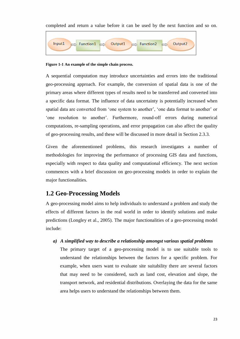
Figure 1-1 An example of the simple chain process. ...................................................... 23
Figure 1-2 The site selection model for identifying a potential school location (Source:
ESRI 2011). ......................................................................................................... 25
2 Processing GIS Data and Functions
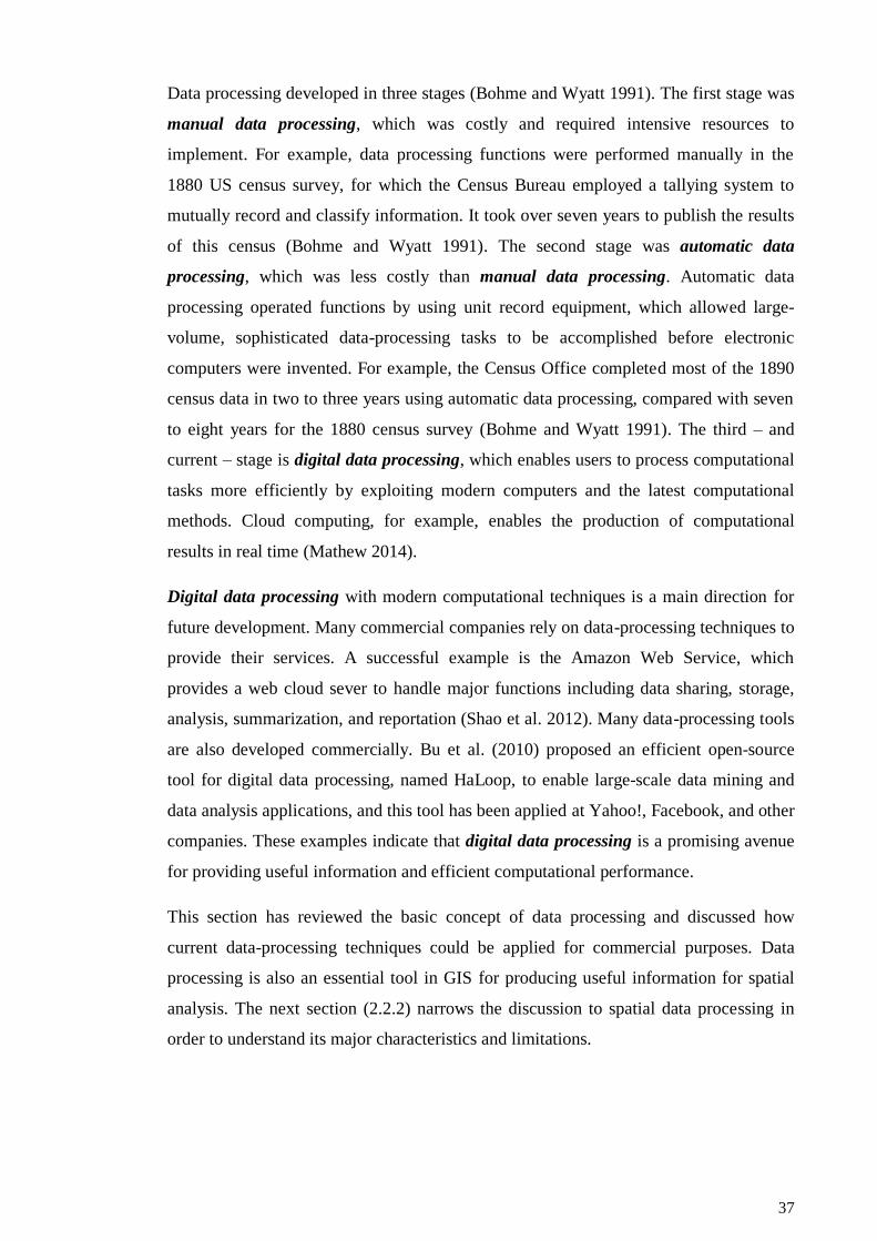
Figure 2-1 An example of a geo-processing model in ModelBuilder. ............................ 39
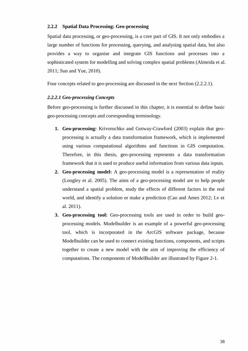
Figure 2-2 The basic components of a simple geo-processing model. ........................... 40
Figure 2-3 Geo-processing example of a simple chain model. ....................................... 40
Figure 2-4 Geo-processing example of a parallel chain model....................................... 41
Figure 2-5 The geo-processing model for location analysis. .......................................... 41
Figure 2-6 The basic strategy of sequential computation. .............................................. 42
Figure 2-7 A conceptual model of uncertainty (after Devillers and Jeansoulin, 2010). . 47
Figure 2-8 A comparison between accuracy and precision (after Lee et al 2015). ......... 47
Figure 2-9 A review of errors in GIS (after Hunter and Beard 1992). ............................ 49
Figure 2-10 Slopes in a raster-based layer. ..................................................................... 52
Figure 2-11 The performance of various algorithms (after Apelbaum 2011). ................ 63
Figure 2-12 An example of a complex geo-processing model. ...................................... 64
Figure 2-13 Region of Interest (ROI) in Land Use. ........................................................ 65
3 Conceptual Model of Combinative Geo-processing (CG) Approach
Figure 3-1 A comparison of a ‘simple chain’ process using the traditional geo-
processing and CG approaches............................................................................ 72
14
Figure 3-2 A comparison of a ‘complex chain’ process using the traditional geo-
processing and CG approaches............................................................................ 74
Figure 3-3 Conceptual model of the CG approach. ........................................................ 75
Figure 3-4 Basic GIS functions included in the CG function library. ............................ 79
Figure 3-5 The generic frameworks of the traditional geo-processing and CG
approaches. .......................................................................................................... 80
4 Case Study Design and Combinative Geo-Processing Implementation Methods
Figure 4- 1 Overview of three typical issues in a complex geo-processing model......... 87
Figure 4- 2 Summary of the experimental case studies used for the development of the
CG approach. ....................................................................................................... 88
Figure 4- 3 Map Overlay function used in the second case study. ................................. 89
Figure 4- 4 A CG function used in the second case study. ............................................. 89
Figure 4- 5 Property Location Planning Model used in the third case study. ................. 90
Figure 4- 6 The Sierpinski triangle (after Weisstein, 2013)............................................ 93
Figure 4- 7 Eager Evaluation algorithm for calculating the mean, variance and standard
deviation for a set of numbers. ............................................................................ 94
Figure 4- 8 Lazy Evaluation algorithm for calculating the mean, variance and standard
deviation for a set of numbers. ............................................................................ 95
Figure 4- 9 IDW implementation steps. ........................................................................ 102
Figure 4- 10 The Selected data for the benchmark process. ......................................... 103
Figure 4- 11 An example of raster math. ...................................................................... 104
Figure 4- 12 The strategy to compare the various GIS tools and CG results................ 104
Figure 4- 13 Raster algebra: Comparison of IDW outcomes. ....................................... 105
Figure 4- 14 The geometry (centroid) of the interpolated grid (a. in ArcGIS; b. in
MapInfo). ........................................................................................................... 108
15
Figure 4- 15 Examples of interpolating sample points in ArcGIS and MapInfo. ......... 109
Figure 4- 16 ArcGIS 9.2 software. ................................................................................ 110
Figure 4- 17 MapInfo 8.5.1 software. ........................................................................... 111
Figure 4- 18 Racket main webpage. .............................................................................. 111
Figure 4- 19 The Racket interface. ................................................................................ 112
Figure 4- 20 Description of the testing computer. ........................................................ 112
Figure 4- 21 Source of the selected LiDAR data. ......................................................... 113
Figure 4- 22 Visualisation of LiDAR sample points and their attributed values (X, Y,
and Z) in 2D. ..................................................................................................... 114
Figure 4- 23 Visualisation of LiDAR sample points in 3D. ......................................... 114
Figure 4- 24 Number of selected LiDAR points and size of the study area in the three
case studies. ....................................................................................................... 115
5 Comparing a Raster Overlay Function between Map Algebra and Combinative
Geo-processing
Figure 5-1 Example of ‘Raster Overlay with Raster’ function (‘Overlay Analysis’, ESRI
ArcGIS Resource Centre Online, 2008). ........................................................... 118
Figure 5-2 Another example of ‘Raster Overlay with Raster’ function (After Madden
2009). ................................................................................................................. 119
Figure 5-3 Case study 1: Geo-processing model (‘Raster Overlay with Raster’
Function). .......................................................................................................... 120
Figure 5-4 ‘Raster Overlay with Raster’ function workflow in traditional geo-processing
(Map Algebra). .................................................................................................. 121
Figure 5-5 ‘Raster Overlay with Raster’ function workflow in the CG approach. ...... 122
Figure 5-6 Reference data (Case study 1). ................................................................... 124
16
Figure 5-7 ‘Raster Overlay with Raster’ function implementation steps (Case study 1).
........................................................................................................................... 126
Figure 5-8 Case study 1: The process of generating the reference layers using R. ...... 127
Figure 5-9 Case study 1: The process of generating the simple layers using ArcGIS and
MapInfo. ............................................................................................................ 127
Figure 5-10 Case study 1: The process of generating the Integrated Reference Layer
(IRL) using R. ................................................................................................... 128
Figure 5-11 Case study 1: The process of generating the Integrated Sample Layer (ISL)
using ArcGIS and MapInfo. .............................................................................. 128
Figure 5-12 Case Study 1: The process of generating the Integrated Sample Layer (ISL)
using the CG approach. ..................................................................................... 129
Figure 5-13 Single reference layer ................................................................................ 130
Figure 5-14 Single sample layer ................................................................................... 131
Figure 5-15 Integrated Reference Layer (1M) generated using R. ............................... 132
Figure 5-16 Integrated Reference Layer (1.5M) generated using R. ............................ 132
Figure 5-17 Integrated Sample Layer (1.5M) generated using ArcGIS....................... 133
Figure 5-18 Integrated Sample Layer (1M) generated using MapInfo. ........................ 133
Figure 5-19 Integrated Sample Layer (1.5M) generated using the CG approach. ........ 133
Figure 5-20 Integrated Sample Layer(1M) generated using the CG approach. ............ 134
Figure 5-21 Raster Algebra: Comparison of the ‘Raster Overlay with Raster’ function
outcomes. ........................................................................................................... 135
6 Implementing a Simple Chain Processing Using the Combinative Geo-
Processing Function
Figure 6-1 The workflow of a generic simple chain processing model. ....................... 140
Figure 6-2 Case study 2: Geo-processing model (Simple chain processing model)..... 140
17
Figure 6-3 Example of elevation matrix used for Slope computation. ......................... 140
Figure 6-4 Case study 2: Simple chain processing model in ArcGIS ModelBuilder. .. 142
Figure 6-5 Case study 2: Simple chain processing model in the CG approach. ........... 143
Figure 6-6 Case study 2: Raw LiDAR point data and case study area (yellow rectangle
in Bing Maps satellite image). ........................................................................... 145
Figure 6-7 Case study 2: Implementation strategy of simple chain processing model. 146
Figure 6-8 Case study 2: The 2,000 sampling locations and the case study area (shown
by the yellow rectangle in Bing Maps satellite image). .................................... 147
Figure 6-9 Case study 2: ArcGIS model for querying slope values from the sampling
locations. ........................................................................................................... 148
Figure 6-10 (a) Slope values of sample points (CG approach). (b) Slope values of
sample points (ArcGIS). .................................................................................... 149
Figure 6-11 Difference in sample slope value results that were produced using the CG
approach and ArcGIS ModelBuilder. ................................................................ 149
Figure 6-12 Case study 2: Monte Carlo Simulation (CG approach results). ................ 152
Figure 6-13 Case study 2: Monte Carlo Simulation (ArcGIS results). ......................... 152
Figure 6-14 Case study 2: Standard deviation on sample locations (CG approach
results). .............................................................................................................. 153
Figure 6-15 Case study 2: Standard deviation on sample locations (ArcGIS results). . 153
Figure 6-16 The slope representation (i.e. raster-based) and the distance shift (i.e. the
cause of distortion) between randomly selected location and grid centre point.
........................................................................................................................... 156
7 Implementing a Complex Chain Processing Model Using Combinative Geo-
processing Function
Figure 7-1 The geo-processing model for identifying a suitable location for a dairy farm
site (After Sujoni and Hardjomidjojo, 2010). ................................................... 160
18
Figure 7-2 Region Of Interest (ROI), which shows the pasture area of the dairy farm
model. ................................................................................................................ 161
Figure 7-3 An example of applying the CG computation priority in a simple geo-
processing model. .............................................................................................. 164
Figure 7-4 The complex chain processing model used in Case study 3. ...................... 166
Figure 7-5 Case study 3: Example of complex chain processing model in ModelBuilder
(ArcGIS). ........................................................................................................... 167
Figure 7-6 Case study 3: Complex chain processing model in the CG approach. ........ 170
Figure 7-7 Case study 3: The structure of the CG function in the complex chain
processing model. .............................................................................................. 172
Figure 7-8 Case study 3: The structure of the CG functions in the complex chain
processing model (assigned to CG computation priority values)...................... 174
Figure 7-9 Case study 3: Raw LiDAR point data (one million points) and case study
area (yellow rectangle on Bing Maps satellite image). ..................................... 177
Figure 7-10 Case study 3: Existing property locations. ................................................ 178
Figure 7-11 Case study 3: Road network represented by vertices. ............................... 178
Figure 7-12 Case study 3: Implementation strategy of complex chain processing model.
........................................................................................................................... 179
Figure 7-13 Outcome of computation task a (‘IDW’ function). .................................. 180
Figure 7-14 Outcome of computation task b (‘Slope’ function). .................................. 180
Figure 7-15 Outcome of computation task c (‘Reclassify’ function). ........................... 181
Figure 7-16 Outcome of computation task d (‘Reclassify (2)’ function). ..................... 181
Figure 7-17 Outcome of computation task e (‘Euclidean Distance’ function). ............ 182
Figure 7-18 Outcome of computation task f (‘Reclassify (3)’ function). ...................... 182
Figure 7-19 Outcome of computation task e (‘Euclidean Distance2’ function). .......... 183
19
Figure 7-20 Outcome of computation task f (‘Reclassify (4)’ function). ..................... 183
Figure 7-21 Case study 3: The final result of the site selection analysis (produced using
ModelBuilder, ArcGIS). .................................................................................... 184
Figure 7-22 Case study 3: The final result of the site selection analysis (produced using
the CG approach using CG computation priority). ........................................... 185
Figure 7-23 Case study 3: the validation process (Computation time). ........................ 187
Figure 7-24 Case study 3: Overall computation time in traditional geo-processing and
the CG approach. ............................................................................................... 188
List of Tables
1. Introduction
Table 1-1 Brief summary of the existing issues concerning the traditional geo-
processing approach. ........................................................................................... 27
Table 1-2 The structure of the thesis. .............................................................................. 30
2 Processing GIS Data and Functions
Table 2- 1 Cause of spatial data errors (Fisher 1999). .................................................... 49
Table 2- 2 Errors due to π values with different accuracies. ........................................... 53
Table 2- 3 A summary of major spatial data models and their relationships with points.
......................................................................................................................................... 57
Table 2- 4 The examples of simplification. .................................................................... 59
Table 2- 5 Examples of functional programming: Maple. ………………………….60
4 Case Study Design and Combinative Geo-Processing Implementation Methods
Table 4- 1 GIS functions and software platforms in Case Study 1. ................................ 92
Table 4- 2 Parameters of GIS functions in Case Study 1. ............................................... 93
20
Table 4- 3 Input dataset for Case Study 1. ...................................................................... 93
Table 4- 4 GIS functions and software platforms in Case Study 2. ................................ 95
Table 4- 5 Parameters of GIS functions in Case Study 2. ............................................... 95
Table 4- 6 Input dataset for Case Study 2. ...................................................................... 96
Table 4- 7 Primary parameters for Monte Carlo simulation in Case Study 2. ................ 96
Table 4- 8 GIS functions and software platforms in Case Study 3. ................................ 97
Table 4- 9 Parameters of GIS functions in Case Study 3. ............................................... 98
Table 4- 10 Input dataset for Case Study 3. .................................................................... 99
Table 4- 11 Primary parameters for Monte Carlo simulation in Case Study 3. ............ 100
Table 4- 12 Basic objects in the Scheme programming language. ............................... 107
Table 4- 13 Common operations in Scheme. ................................................................ 108
5 Comparing a Raster Overlay Function between Map Algebra and Combinative
Geo-processing
Table 5-1 Statistical analysis results. ............................................................................ 136
6 Implementing a Simple Chain Processing Using the Combinative Geo-
Processing Function
Table 6-1 Case study 2: A comparison of variance and standard deviation. ................ 154
Table 6-2 Example of round-off errors in numerical computation. .............................. 155
7 Implementing a Complex Chain Processing Model Using Combinative Geo-
processing Function
Table 7-1 A summary of GIS functions in the complex chain processing model. ....... 169
Table 7-2 Case study 3: Input data volume of the functions......................................... 175
Table 7-3 The statistical results of overall computation time between the ArcGIS and
CG approach using CG computation priority (Unit: Second). .......................... 189
21
List of Acronyms
CG: Combinative Geo-processing
DEM: Digital Elevation Model
DTM: Digital Terrain Model
GIS: Geographical Information Systems
GRASS: Geographic Resources Analysis Support System
GUI: Graphical User Interface
IDW: Inverse Distance Weighting
INSIDE: Interactive Numeric and Spatial Information Data Engine
IRL: Integrated Reference Layer
ISL: Integrated Sample Layer
LiDAR: Light Detection And Ranging
NDVI: Normalised Difference Vegetation Model
RAM: Random Access Memory
ROI: Region of Interest
RS: Remote Sensing
SQL: Structured Query Language
SYMAP: Synteny Mapping and Analysis Program
TIN: Triangulated Irregular Networks
22
1. Introduction
1.1 Background
Geographical information systems (GIS) form a powerful set of spatial analysis tools,
where spatial data processing contributes significantly to the quality of the information
and critically affects a GIS user’s ability to carry out reliable and valid analysis. In
principle, spatial data processing provides a comprehensive computation progress,
including input data, functions operating on the input data, and the output or
visualisation of the results. Spatial data processing components can be linked together in
order to build different types of geo-processing models, which can then be used for
more advanced spatial analyses within various contexts, such as urban planning, climate
modelling, utility network management and transport network analysis.
Due to the rapid development of GIS technologies, various implementation approaches
and tools for spatial data processing are already available within GIS software, with one
of the most common approaches being geo-processing. This is based upon a framework
of data transformation, which allows users to interpret data and functions obtained from
different resources (Krivoruchko and Gotway-Crawford, 2003). Geo-processing tools
were first developed and applied in the UK and US in the 1950s in order to reduce map
production and maintenance costs (Vulera, 2011). Currently, geo-processing is a
popular approach within GIS for decision-making and risk assessment purposes due to
the large number of functions provided, such as the integration of geographical features,
features selection and analysis, topology processing, raster processing, and spatial data
conversion (Sommer and Wade, 2006).
A common characteristic of the traditional geo-processing approach is the sequential
computation for implementing a set of functions or a geo-processing model, and Figure
1-1 displays a sequential computation in a simple chain processing model. The system
initially loads ‘Input Data1’ into the function ‘Funtion1’, which yields the output
‘Output1’; ‘Output1’ is then used as input data for the next function ‘Function2’, which
returns the final result ‘Ouput2’. This sequential computation strategy is applied in the
traditional geo-processing approach for the implementation of various geo-processing
models mainly due to the fact that many GIS software packages have been developed
using imperative programming languages (e.g. Java and C++), where a function must be
23
completed and return a value before it can be used by the next function and so on.
Figure 1-1 An example of the simple chain process.
A sequential computation may introduce uncertainties and errors into the traditional
geo-processing approach. For example, the conversion of spatial data is one of the
primary areas where different types of results need to be transferred and converted into
a specific data format. The influence of data uncertainty is potentially increased when
spatial data are converted from ‘one system to another’, ‘one data format to another’ or
‘one resolution to another’. Furthermore, round-off errors during numerical
computations, re-sampling operations, and error propagation can also affect the quality
of geo-processing results, and these will be discussed in more detail in Section 2.3.3.
Given the aforementioned problems, this research investigates a number of
methodologies for improving the performance of processing GIS data and functions,
especially with respect to data quality and computational efficiency. The next section
commences with a brief discussion on geo-processing models in order to explain the
major functionalities.
1.2 Geo-Processing Models
A geo-processing model aims to help individuals to understand a problem and study the
effects of different factors in the real world in order to identify solutions and make
predictions (Longley et al., 2005). The major functionalities of a geo-processing model
include:
a) A simplified way to describe a relationship amongst various spatial problems
The primary target of a geo-processing model is to use suitable tools to
understand the relationships between the factors for a specific problem. For
example, when users want to evaluate site suitability there are several factors
that may need to be considered, such as land cost, elevation and slope, the
transport network, and residential distributions. Overlaying the data for the same
area helps users to understand the relationships between them.
24
b) To solve problems, find potential patterns, and support decision-making
A geo-processing model provides a powerful tool for manipulating different
types of GIS data and functions in order to answer questions such as ‘where is
the best location?’ Consequently, the results will help users to understand
different types of problems in the real world.
c) To provide an assumption or prediction
Many successful applications have been created for modelling environmental
problems and for making predictions. For example, when predicting areas where
flooding may be an issue, users need to assess the amount of rainfall, acquire
information about river discharges, and utilise a terrain model.
A geo-processing model may involve different types of GIS data and functions in order
to solve complex spatial problems, and a geo-processing tool provides a useful way to
implement and manipulate various geo-processing models. Consequently, different
spatial questions can be answered using geo-processing tools, such as ‘Where is the best
location to live?’ or ‘What spatial features does this region include?’
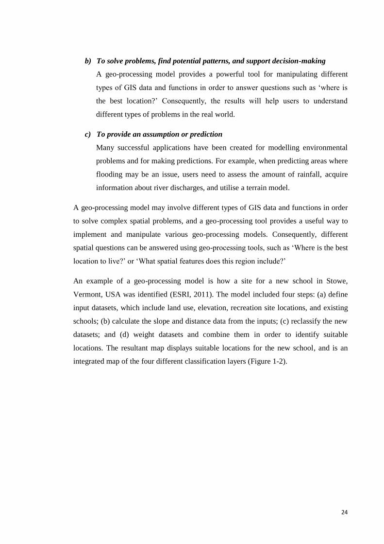
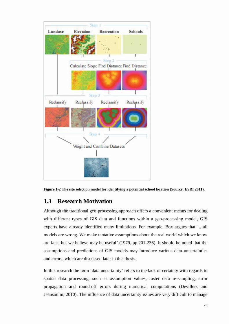
An example of a geo-processing model is how a site for a new school in Stowe,
Vermont, USA was identified (ESRI, 2011). The model included four steps: (a) define
input datasets, which include land use, elevation, recreation site locations, and existing
schools; (b) calculate the slope and distance data from the inputs; (c) reclassify the new
datasets; and (d) weight datasets and combine them in order to identify suitable
locations. The resultant map displays suitable locations for the new school, and is an
integrated map of the four different classification layers (Figure 1-2).
25
Figure 1-2 The site selection model for identifying a potential school location (Source: ESRI 2011).
1.3 Research Motivation
Although the traditional geo-processing approach offers a convenient means for dealing
with different types of GIS data and functions within a geo-processing model, GIS
experts have already identified many limitations. For example, Box argues that ‘.. all
models are wrong. We make tentative assumptions about the real world which we know
are false but we believe may be useful’ (1979, pp.201-236). It should be noted that the
assumptions and predictions of GIS models may introduce various data uncertainties
and errors, which are discussed later in this thesis.
In this research the term ‘data uncertainty’ refers to the lack of certainty with regards to
spatial data processing, such as assumption values, raster data re-sampling, error
propagation and round-off errors during numerical computations (Devillers and
Jeansoulin, 2010). The influence of data uncertainty issues are very difficult to manage
26
within the traditional geo-processing approach, as most geo-processing models are
calculated straightforwardly and without the progress of data quality control. Therefore,
many GIS users apply spatial data analysis using the traditional geo-processing
approach under the assumption that data processing is entirely error free (Burrough and
McDonnell, 1998). However, to further clarify the importance of errors in this context,
consider the following geo-processing scenarios and their associated data quality
problems:
Geo-processing operations often produce results that are generated by
aggregating or disaggregating form input datasets. A common example is the
application of Digital Elevation Model (DEM) data. With the aim of integrating
geographical information, DEM data are often upscaled or downscaled to
provide estimated elevation values for a particular scale, and during this process
spatial interpolation methods, such as Kriging and inverse distance weight
(IDW), are frequently employed for re-sampling raster data. However, the
interpolation methods provide only estimated values for attributes associated
with the newly created features, not the real values. Therefore, how to control
data quality and the impact of estimated values during geo-processing should be
considered.
Vectorisation is a geo-processing function for converting a raster image to vector
data. In common GIS tools, such as ArcGIS, the vectorisation function includes
two different algorithms: (a) to generate vector lines along the centre of the
raster linear elements; and (b) to generate vector lines at the border of the
connected cells. However, which algorithm represents more closely the true
features and what is the impact of these algorithms on subsequent computations?
Raster data provide a simple data structure for representing spatial information.
However, the resolution of the raster significantly affects the data quality. In a
raster image with a resolution of five metres, any points located within the same
grid will be represented as the same value even they are five meters apart. What
will happen if users apply this image as the input dataset to generate a new
output and how are errors propagated in this context?
These scenarios indicate that data quality problems influence different types of geo-
processing models. Moreover, there are a number of existing problems in spatial data
processing:
27
Data conversion: The main characteristic of geo-processing is to link various
functions into an integrated model, whereby data conversion is a basic process to
transfer the results from different type of functions. When spatial data are
converted, there is the potential of increasing the error in the resulting data
(Devillers and Jeansoulin, 2006).
Numerical computation: This is widely used by current GIS software packages,
such as ArcGIS, MapInfo, GRASS, and Manifold, for data processing. This
method uses numerical approximation algorithms to represent mathematical
equations, and it is worth noting that there is an error between approximated
values and true values. The accumulated errors in traditional geo-processing may
directly affect the quality of the final result (Hildebrand, 1987).
Error propagation: One of the most important functionalities of geo-processing
is to derive new attributes from attributes already held within a GIS database.
However, no data stored in a GIS database are truly error-free and no GIS tools
exist that can mitigate the effect of error propagation in a reliable manner
(Heuvelink, 2006).
Cost of large computation resources: In addition to data quality, the
computational efficiency when processing a large spatial dataset has also
attracted attention in recent years. There are many potential issues concerning
current geo-processing tools with respect to computational efficiency, for
example, spatial data always needs to be processed by entire region, not by the
specific request.
Finally, the influence of data uncertainties and computational efficiency during data
processing may cause additional and more critical problems (e.g. system damage) when
such geo-processing models are used to solve spatial problems in the real world. For
example, the interpolation method (e.g. IDW) in GIS is commonly used to produce
DEM data in order to describe land surface features (i.e. elevation values), and many
engineering applications rely on DEM data (e.g. hydrological system, infrastructure
network, property construction, and utility services). Therefore, if DEM data produced
by a geo-processing model includes a significant level of data uncertainties or errors,
then there is the potential for many issues to occur following the application of such
data, e.g. flooding, infrastructure system failures, transport network system failures, or
water supply system damage.
28
1.4 Research Aims and Objectives
A number of existing problems concerning the traditional geo-processing approach have
been briefly discussed in the previous section. Further details on the causes of these
problems and their effects on spatial data processing will be discussed in Sections 2.3
and 2.4. Based on their influences on spatial data processing, the current issues
concerning geo-processing can be classified into two categories: data quality and
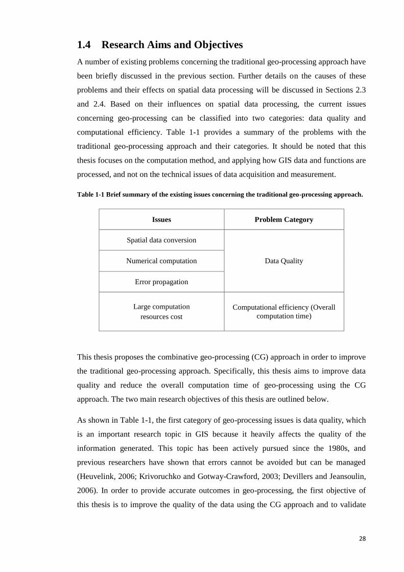
computational efficiency. Table 1-1 provides a summary of the problems with the
traditional geo-processing approach and their categories. It should be noted that this
thesis focuses on the computation method, and applying how GIS data and functions are
processed, and not on the technical issues of data acquisition and measurement.
Table 1-1 Brief summary of the existing issues concerning the traditional geo-processing approach.
Issues Problem Category
Spatial data conversion
Data Quality Numerical computation
Error propagation
Large computation
resources cost
Computational efficiency (Overall
computation time)
This thesis proposes the combinative geo-processing (CG) approach in order to improve
the traditional geo-processing approach. Specifically, this thesis aims to improve data
quality and reduce the overall computation time of geo-processing using the CG
approach. The two main research objectives of this thesis are outlined below.
As shown in Table 1-1, the first category of geo-processing issues is data quality, which
is an important research topic in GIS because it heavily affects the quality of the
information generated. This topic has been actively pursued since the 1980s, and
previous researchers have shown that errors cannot be avoided but can be managed
(Heuvelink, 2006; Krivoruchko and Gotway-Crawford, 2003; Devillers and Jeansoulin,
2006). In order to provide accurate outcomes in geo-processing, the first objective of
this thesis is to improve the quality of the data using the CG approach and to validate
29
the results by comparing them with the traditional geo-processing approach. This
objective leads to the following research questions:
How can the data quality be improved in the CG approach?
This requires an exploration of the methods that can be applied in the CG
approach to improve data quality and also how these methods can be
implemented in the CG approach.
How can the results of the CG approach be validated?
The second category of the problems illustrated in the Table 1-1 is the computational
efficiency of geo-processing. GIS is widely used in various fields, such as
transportation, environmental modelling, asset management, and citizen science.
Nevertheless, computational efficiency is a major concern for the development of GIS
tools as the size of spatial datasets and the complexity of spatial problems are
dramatically increasing (Brown and Coenen, 2000). Moreover, the CG approach is
employed to process large geographical data and complex GIS functions then there is
the potential risk of heavy computation time costs, as many computation rules (e.g.
symbolic computation) will be used to improve the data quality and may potentially
extend the overall computation time. Therefore, the second objective of this thesis is to
improve the overall computation time of geo-processing using the CG approach and to
validate the results by comparing them with the traditional geo-processing approach. To
address this objective the following research questions should be explored:
What methods can be applied to reduce the overall computation time in geo-
processing?
How can computer resources (e.g. computer memory and CPU) be efficiently
used for the geo-processing computations?
How can redundant computations be avoided in a geo-processing model?
How can the results from the CG approach be validated?
1.5 The Structure of Thesis
The CG approach is a multidisciplinary concept and consequently this research includes
many important topics, such as functional programming, data quality, computational
efficiency, and so on. Therefore, it is necessary at this stage to provide a brief overview
of the thesis outline.
30
The research is organised into four steps for the development of the CG approach:
Step 1: An extensive review of the traditional processing of GIS data and
functions, and potential methods that can be applied in the CG approach
(Chapter 2).
The major characteristics of the traditional geo-processing approach and their
limitations are investigated in this step in order to identify the major problems. A
preparation phase has been previously undertaken, which involved a study of the
basic methods related to the CG approach in order to improve the traditional geo-
processing approach.
Step 2: Design of a framework for the CG approach and the basic methodologies
for the implementation of the CG approach (Chapters 3 and 4).
A conceptual framework for the CG approach is required in order to answer the
research questions. This research needs to build a set of formulae to create the CG
functions and function-based layers, before establishing a set of computation rules
to manipulate the CG functions and function-based layers.
Step 3: Design of a set of case studies to demonstrate how the CG approach can
be implemented and the evaluation of the results (Chapter 4).
A set of scenarios is designed for the development of the CG approach. These
scenarios are focused on the basic questions of geo-processing, such as how to
generate spatial information from functional layers.
Step 4: Implementations and analysis of the results (Chapters 5 to 7).
The case studies are implemented and a comprehensive comparison of the results is
performed as the last step of this research. The investigation attempts to answer the
research questions by discussing how the influence of data uncertainties is reduced
in the CG approach and how the computational efficiency is improved.
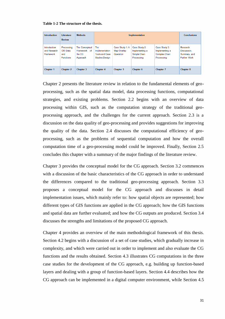
Table 1-2 illustrates the structure of the thesis in relation to the research steps and
objectives in a diagrammatic form.
31
Table 1-2 The structure of the thesis.
Chapter 2 presents the literature review in relation to the fundamental elements of geo-
processing, such as the spatial data model, data processing functions, computational
strategies, and existing problems. Section 2.2 begins with an overview of data
processing within GIS, such as the computation strategy of the traditional geo-
processing approach, and the challenges for the current approach. Section 2.3 is a
discussion on the data quality of geo-processing and provides suggestions for improving
the quality of the data. Section 2.4 discusses the computational efficiency of geo-
processing, such as the problems of sequential computation and how the overall
computation time of a geo-processing model could be improved. Finally, Section 2.5
concludes this chapter with a summary of the major findings of the literature review.
Chapter 3 provides the conceptual model for the CG approach. Section 3.2 commences
with a discussion of the basic characteristics of the CG approach in order to understand
the differences compared to the traditional geo-processing approach. Section 3.3
proposes a conceptual model for the CG approach and discusses in detail
implementation issues, which mainly refer to: how spatial objects are represented; how
different types of GIS functions are applied in the CG approach; how the GIS functions
and spatial data are further evaluated; and how the CG outputs are produced. Section 3.4
discusses the strengths and limitations of the proposed CG approach.
Chapter 4 provides an overview of the main methodological framework of this thesis.
Section 4.2 begins with a discussion of a set of case studies, which gradually increase in
complexity, and which were carried out in order to implement and also evaluate the CG
functions and the results obtained. Section 4.3 illustrates CG computations in the three
case studies for the development of the CG approach, e.g. building up function-based
layers and dealing with a group of function-based layers. Section 4.4 describes how the
CG approach can be implemented in a digital computer environment, while Section 4.5
32
describes the selected data that are used in the case studies. Finally, Section 4.6
summarises the main issues that are discussed in this chapter.
A set of experiments was designed for this research through a series of case studies. The
first case study is explained in Chapter 5, and investigates a multi-layer overlay
operation using the CG approach and map algebra. Section 5.2 discusses the ‘Raster
Overlay with Raster’ function. Section 5.3 explains how the ‘Raster Overlay with
Raster’ function is implemented using map algebra, which is commonly used within the
context of the traditional geo-processing approach in order to overlay more than one
raster data layers. Section 5.4 presents the datasets and more specifically the reference
and sample data that are used in the case study. Section 5.5 describes the
implementation strategy for the ‘Raster Overlay with Raster’ function and Section 5.6
presents the results. Section 5.7 provides a more detailed comparison of the map algebra
and the CG approach results, and Section 5.8 discusses the differences. Finally, Section
5.9 discusses the main issues and problems that are revealed in the first case study.
Chapter 6 validates the quality of a simple chain processing model. Section 6.2 starts
with a discussion of a primitive simple chain processing model and describes the geo-
processing model that it is used in this case study. Section 6.3 introduces the two
different approaches that can be used for the implementation of any simple chain
processing models: the traditional geo-processing approach using the ModelBuilder tool
in ArcGIS and the CG approach. Section 6.4 presents the datasets that are used in this
second case study. Section 6.5 discusses the implementation strategy for executing the
simple chain processing model and Section 6.6 presents the results. In Section 6.7 the
Monte Carlo simulation is used to compare the influences of data uncertainties in both
simple chain processing model implementations. Section 6.8 discusses the differences
between the various Monte Carlo simulation outcomes and Section 6.9 summarises the
main issues that are discussed in the second case study.
Chapter 7 discusses how the computational efficiency of geo-processing can be
improved in the CG approach. Section 7.2 reviews the implications of an inefficient
computation strategy in geo-processing and discusses the concepts of computation
flexibility and computation sequence. Section 7.3 introduces the concept of CG
computation priority, which aims to reduce the overall computation time of geo-
processing through the use of an improved computation strategy. Section 7.4 discusses
the complex chain processing model that is applied in the third case study and Section
7.5 describes how the model is implemented in the traditional geo-processing and the

33
CG approaches using computation priority. Section 7.6 presents the datasets that are
used in the third case study. Section 7.7 discusses in detail the implementation and
strategy for executing the complex chain processing model using the two different geo-
processing approaches and Section 7.8 presents the results. Section 7.9 compares the
implementation results on overall computation time using the Monte Carlo simulation
method. Finally, Section 7.10 concludes with a summary of the main issues and
findings discussed in this third case study.
Chapter 8 concludes the thesis by discussing and summarising the research undertaken.
Section 8.1 presents a brief overview and Section 8.2 discusses the major research
findings. Section 8.3 discusses the contribution of this thesis, whilst Section 8.4 reviews
the limitations of the CG approach development, and Section 8.5 proposes the direction
of future research.
34
2 Processing GIS Data and Functions
2.1 Introduction
Data processing involves extracting meaningful information from raw data, which is
then used for data analysis and decision-making (French 1996). Data processing has
been a topic of research in various applications, such as commercial data processing and
data analysis, and is widely accepted as a critical part of addressing complex problems.
In GIS, spatial data processing, known as ‘geo-processing’, includes various
computational tasks, such as spatial analysis, GIS visualisation and geostatistics (Karimi
et al. 2011). The aim of geo-processing is the collection and manipulation of spatial data
to produce useful information and solve complex spatial problems (Niu et al. 2013).
Geo-processing relies on a computational framework consisting of spatial functions and
models, which traditionally are applied in sequence. Such a framework usually lacks
mechanisms for data quality control and effective management of computation time.
Moreover, some basic methods involved in geo-processing (e.g. spatial data
representation and basic computation) may introduce uncertainties and errors through
approximations and error propagation. This thesis addresses the implications of this
framework, which we call the ‘traditional geo-processing approach’, and proposes a
new approach – the ‘Combinative Geo-processing (CG) approach’ – aimed at
improving the data quality and computational efficiency of geo-processing.
The proposed CG approach is realised using a point-based spatial data model, symbolic
computation, and functional layers in order to improve data quality. By describing
features of both discrete objects and continuous fields, the point-based spatial data
model aims to reduce the complexity of GIS representations and avoid problems with
data quality that can arise from raster resolution and spatial data conversion. Symbolic
computation and functional layers minimise the effects of data uncertainty and error
propagation on geo-processing results. Additionally, the proposed CG approach
employs a priority-based computation strategy that reduces the entire time-cost of a geo-
processing model and thereby improves computational efficiency.
This chapter reviews problems with data quality and computational efficiency that arise
from the traditional geo-processing approach, and discusses how these problems can be
improved. First, basic concepts of spatial data processing are introduced; these then
enable an exploration of traditional geo-processing problems which influence data
35
quality and computational efficiency. Lastly, potential ways to improve the traditional
geo-processing approach are discussed.
Section 2.2 discusses the major characteristics and implications of the traditional geo-
processing approach. Section 2.2.1 reviews the concept of data processing and enables
us to understand its fundamental elements. In Section 2.2.2 the discussion narrows
down to spatial data processing and describes how a geo-processing model is built and
executed. Section 2.2.3 summarises and concludes with the major characteristics of the
traditional geo-processing approach and its challenges.
Section 2.3 discusses major data-quality problems that arise in traditional geo-
processing and provides evidence of scope for improvement. Section 2.3.1 defines
common data-quality terms that are used in this thesis. Section 2.3.2 reviews common
errors in GIS, and Section 2.3.3 discusses the specific data-quality problems seen in
geo-processing, including with spatial data representation and geo-processing
computation. These two methods are singled out because they have many existing data-
quality problems affecting on the traditional geo-processing approach, such as data
uncertainty and error propagation. Section 2.3.4 discusses methods that are applicable to
the CG approach for improving geo-processing, particularly by reducing the influence
of data-quality problems.
Section 2.4 discusses another issue – computational efficiency – with the traditional
geo-processing approach, as this provides further evidence for the necessity of
improving the traditional geo-processing approach. Section 2.4.1 reviews common
computational efficiency definitions that are used in this research. Then, Section 2.4.2
discusses existing problems with computational efficiency in a complex geo-processing,
including ‘waiting’ functions and unnecessary computations. These two problems are
selected because they can extend the entire computation time of a geo-processing model.
Section 2.4.3 concludes by contrasting the traditional geo-processing approach with
improvements in computational efficiency achieved by the CG approach.
Section 2.5 summarises the main points discussed and concludes with suggestions for
improving the data quality and computational efficiency of geo-processing.
2.2 Data Processing In GIS
To understand the fundamental methods and basic characteristics of data processing,
this chapter presents a historical review of the development of data processing, focusing
36
on both manual and automatic processing. Then the research narrows down to spatial
data processing, i.e. geo-processing, and its major functionalities, in order to explain
how spatial data and functions are manipulated in GIS. Furthermore, the traditional geo-
processing approach and its challenges are discussed in this section.
2.2.1 Data Processing Overview
As the real world becomes more complex, various questions need to be investigated.
For example, global networked risks (e.g. economic, environmental, health, and food)
are extremely complicated, as they are globally connected and influence each other
(Helbing 2013). In order to address complicated problems and support useful
information for decision making, there is a need to organize, manipulate, and analyse
large amounts of data using different data-processing tools (French 1996). Consequently,
this section discusses the basic concept of data processing.
Most data processing tools include "a group of interrelated components that seek the
attainment of a common goal by accepting inputs and producing outputs in an
organised process" (O'Brien 1986, p. 66). In principle, a data processing system has
three components. The first component is the data input. Some popular functions of
data input include data capture and collection in preparation for processing. The second
component is the data processing, which includes functions such as data sorting,
classification, interpolation, assumptions, and valuation. Sorting and classification
arrange items or data in a specific order or in different sets for processing; interpolation
and assumptions provide a way to calculate unknown information from captured data;
evaluation tries to ensure the manipulated data is correct, reliable, and useful. The third
component is the output of information, and common processing functions here include
data aggregation, presentation, summarization, and reportation. Data aggregation
integrates different outputs into a comprehensive result, for example by combining
different data layers into a final single layer. Data validation ensures that the
manipulated data are correct, reliable, and useful for problem-solving. Data presentation
is used to illustrate the results of the data processing. Summarisation and reportation
capture the main features of the datasets and results. Taken together, the three
components provide the basic structure of the data processing framework and can help
users to build their own data-processing system, such as the conceptual framework for
the CG approach, discussed in Chapter 3.
37
Data processing developed in three stages (Bohme and Wyatt 1991). The first stage was
manual data processing, which was costly and required intensive resources to
implement. For example, data processing functions were performed manually in the
1880 US census survey, for which the Census Bureau employed a tallying system to
mutually record and classify information. It took over seven years to publish the results
of this census (Bohme and Wyatt 1991). The second stage was automatic data
processing, which was less costly than manual data processing. Automatic data
processing operated functions by using unit record equipment, which allowed large-
volume, sophisticated data-processing tasks to be accomplished before electronic
computers were invented. For example, the Census Office completed most of the 1890
census data in two to three years using automatic data processing, compared with seven
to eight years for the 1880 census survey (Bohme and Wyatt 1991). The third – and
current – stage is digital data processing, which enables users to process computational
tasks more efficiently by exploiting modern computers and the latest computational
methods. Cloud computing, for example, enables the production of computational
results in real time (Mathew 2014).
Digital data processing with modern computational techniques is a main direction for
future development. Many commercial companies rely on data-processing techniques to
provide their services. A successful example is the Amazon Web Service, which
provides a web cloud sever to handle major functions including data sharing, storage,
analysis, summarization, and reportation (Shao et al. 2012). Many data-processing tools
are also developed commercially. Bu et al. (2010) proposed an efficient open-source
tool for digital data processing, named HaLoop, to enable large-scale data mining and
data analysis applications, and this tool has been applied at Yahoo!, Facebook, and other
companies. These examples indicate that digital data processing is a promising avenue
for providing useful information and efficient computational performance.
This section has reviewed the basic concept of data processing and discussed how
current data-processing techniques could be applied for commercial purposes. Data
processing is also an essential tool in GIS for producing useful information for spatial
analysis. The next section (2.2.2) narrows the discussion to spatial data processing in
order to understand its major characteristics and limitations.
38
2.2.2 Spatial Data Processing: Geo-processing
Spatial data processing, or geo-processing, is a core part of GIS. It not only embodies a
large number of functions for processing, querying, and analysing spatial data, but also
provides a way to organise and integrate GIS functions and processes into a
sophisticated system for modelling and solving complex spatial problems (Almeida et al.
2011; Sun and Yue, 2010).
Four concepts related to geo-processing are discussed in the next Section (2.2.2.1).
2.2.2.1 Geo-processing Concepts
Before geo-processing is further discussed in this chapter, it is essential to define basic
geo-processing concepts and corresponding terminology.
1. Geo-processing: Krivoruchko and Gotway-Crawford (2003) explain that geo-
processing is actually a data transformation framework, which is implemented
using various computational algorithms and functions in GIS computation.
Therefore, in this thesis, geo-processing represents a data transformation
framework that it is used to produce useful information from various data inputs.
2. Geo-processing model: A geo-processing model is a representation of reality
(Longley et al. 2005). The aims of a geo-processing model are to help people
understand a spatial problem, study the effects of different factors in the real
world, and identify a solution or make a prediction (Cao and Ames 2012; Lv et
al. 2011).
3. Geo-processing tool: Geo-processing tools are used in order to build geo-
processing models. Modelbuilder is an example of a powerful geo-processing
tool, which is incorporated in the ArcGIS software package, because
Modelbuilder can be used to connect existing functions, components, and scripts
together to create a new model with the aim of improving the efficiency of
computations. The components of ModelBuilder are illustrated by Figure 2-1.
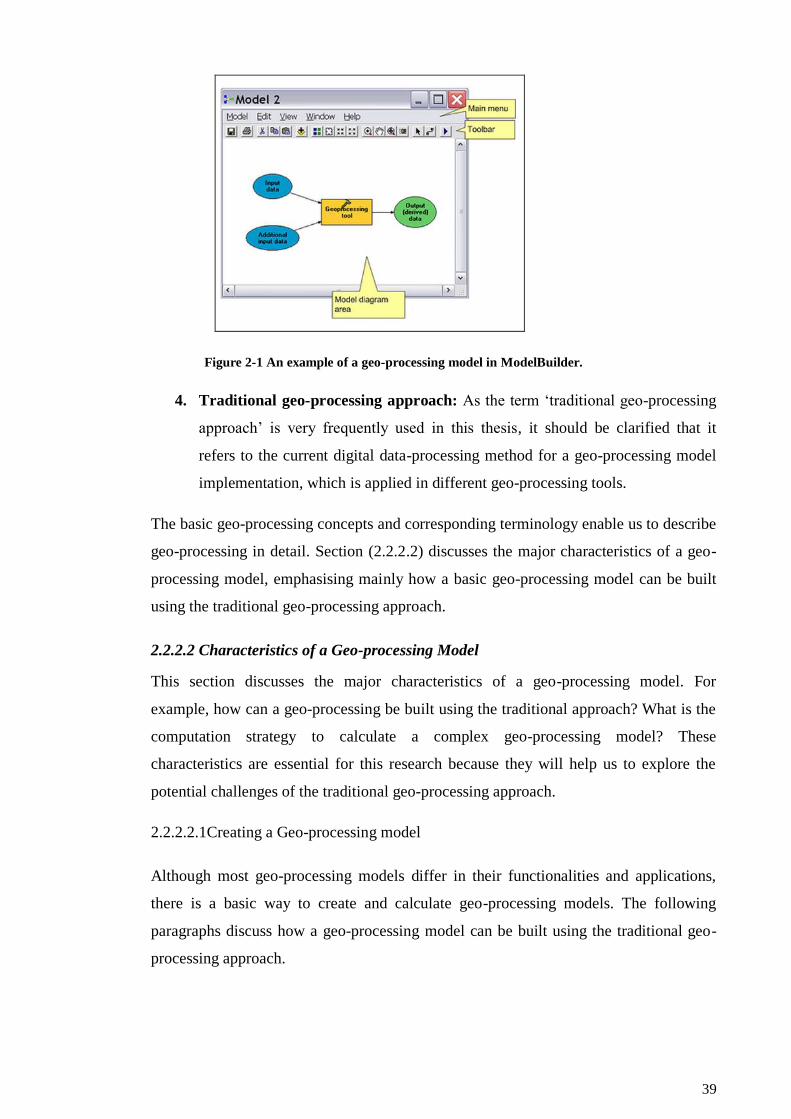
39
Figure 2-1 An example of a geo-processing model in ModelBuilder.
4. Traditional geo-processing approach: As the term ‘traditional geo-processing
approach’ is very frequently used in this thesis, it should be clarified that it
refers to the current digital data-processing method for a geo-processing model
implementation, which is applied in different geo-processing tools.
The basic geo-processing concepts and corresponding terminology enable us to describe
geo-processing in detail. Section (2.2.2.2) discusses the major characteristics of a geo-
processing model, emphasising mainly how a basic geo-processing model can be built
using the traditional geo-processing approach.
2.2.2.2 Characteristics of a Geo-processing Model
This section discusses the major characteristics of a geo-processing model. For
example, how can a geo-processing be built using the traditional approach? What is the
computation strategy to calculate a complex geo-processing model? These
characteristics are essential for this research because they will help us to explore the
potential challenges of the traditional geo-processing approach.
2.2.2.2.1Creating a Geo-processing model
Although most geo-processing models differ in their functionalities and applications,
there is a basic way to create and calculate geo-processing models. The following
paragraphs discuss how a geo-processing model can be built using the traditional geo-
processing approach.
40
There are three basic steps to build a geo-processing model with the traditional geo-
processing approach. First, the most basic element of a geo-processing model comprises
three components: the input data, the GIS function itself, and the output (Figure 2-2).
Figure 2-2 The basic components of a simple geo-processing model.
Second, this simple geo-processing model could be used to build more complicated geo-
processing models, such as simple and parallel chain models. Figure 2-3 illustrates a
simple chain model, in which the output of one model becomes the input of the resulting
model. As it can be seen by Figure 2-3 the first model applies an inverse distance
weighting (IDW) function to produce a continuous elevation surface (i.e. ‘Output1’)
from the input of ‘Raw LiDAR Points’. The derived raster layer becomes the input data
for the next model, which classifies the input data based on a set of conditions.
Figure 2-3 Geo-processing example of a simple chain model.
Figure 2-4 illustrates a parallel chain model that has the same input data (i.e.
‘Continuous Elevation Surface’) and produces two outputs, the ‘Slope Map’ and
‘Classified Map’. It should be noted that the direction of the parallel chain model could
be reversed, which means it could produce a single output from many functions and
input datasets.
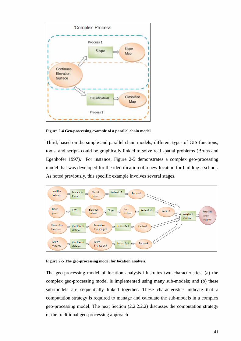
41
Figure 2-4 Geo-processing example of a parallel chain model.
Third, based on the simple and parallel chain models, different types of GIS functions,
tools, and scripts could be graphically linked to solve real spatial problems (Bruns and
Egenhofer 1997). For instance, Figure 2-5 demonstrates a complex geo-processing
model that was developed for the identification of a new location for building a school.
As noted previously, this specific example involves several stages.
Figure 2-5 The geo-processing model for location analysis.
The geo-processing model of location analysis illustrates two characteristics: (a) the
complex geo-processing model is implemented using many sub-models; and (b) these
sub-models are sequentially linked together. These characteristics indicate that a
computation strategy is required to manage and calculate the sub-models in a complex
geo-processing model. The next Section (2.2.2.2.2) discusses the computation strategy
of the traditional geo-processing approach.
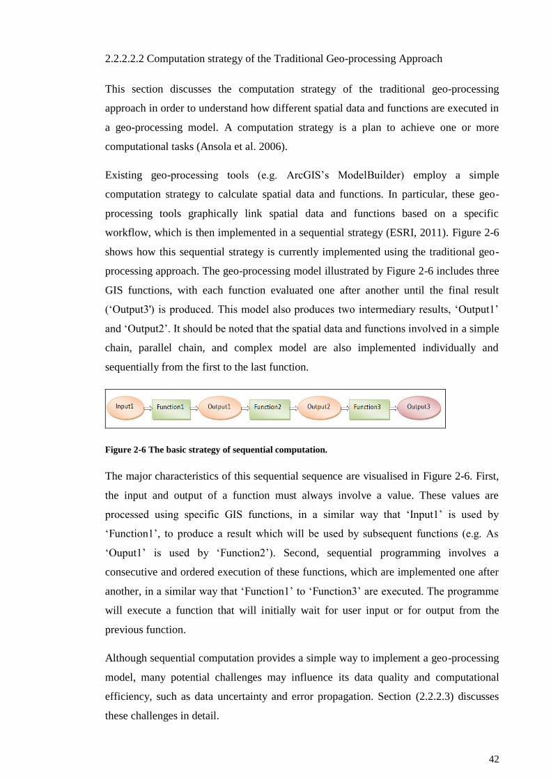
42
2.2.2.2.2 Computation strategy of the Traditional Geo-processing Approach
This section discusses the computation strategy of the traditional geo-processing
approach in order to understand how different spatial data and functions are executed in
a geo-processing model. A computation strategy is a plan to achieve one or more
computational tasks (Ansola et al. 2006).
Existing geo-processing tools (e.g. ArcGIS’s ModelBuilder) employ a simple
computation strategy to calculate spatial data and functions. In particular, these geo-
processing tools graphically link spatial data and functions based on a specific
workflow, which is then implemented in a sequential strategy (ESRI, 2011). Figure 2-6
shows how this sequential strategy is currently implemented using the traditional geo-
processing approach. The geo-processing model illustrated by Figure 2-6 includes three
GIS functions, with each function evaluated one after another until the final result
(‘Output3') is produced. This model also produces two intermediary results, ‘Output1’
and ‘Output2’. It should be noted that the spatial data and functions involved in a simple
chain, parallel chain, and complex model are also implemented individually and
sequentially from the first to the last function.
Figure 2-6 The basic strategy of sequential computation.
The major characteristics of this sequential sequence are visualised in Figure 2-6. First,
the input and output of a function must always involve a value. These values are
processed using specific GIS functions, in a similar way that ‘Input1’ is used by
‘Function1’, to produce a result which will be used by subsequent functions (e.g. As
‘Ouput1’ is used by ‘Function2’). Second, sequential programming involves a
consecutive and ordered execution of these functions, which are implemented one after
another, in a similar way that ‘Function1’ to ‘Function3’ are executed. The programme
will execute a function that will initially wait for user input or for output from the
previous function.
Although sequential computation provides a simple way to implement a geo-processing
model, many potential challenges may influence its data quality and computational
efficiency, such as data uncertainty and error propagation. Section (2.2.2.3) discusses
these challenges in detail.
43
2.2.2.3 Identifying the Challenges in the Traditional Geo-processing Approach
While the traditional geo-processing approach with sequential computation is used to
process spatial data and functions, it incorporates many challenges, which are discussed
here to illustrate that there is a need to improve the traditional geo-processing approach
2.2.2.3.1 Data Quality
Data quality is a major challenge for the development of the traditional geo-processing
approach as different data-quality issues can cause many problems in data processing.
Spatial representation is a fundamental issue in geo-processing, as spatial features must
be correctly represented in a digital environment to produce meaningful information
(Komarkova et al. 2011, Komarkova et al. 2012). However, many data-quality issues
arise in spatial representation methods that are applied in the traditional geo-processing
approach, especially in relation to raster data. Braunisch and Suchant (2010) state that
there is a trade-off between the size of raster data and the precision with which spatial
features can be represented, so spatial data quality can be reduced due to limited
computer memory. Haklay (2004) observes that because spatial attributes are
represented as raster layers with an arbitrary resolution, many potential data
uncertainties exist in raster data. Kienzle (2004) claims that many types of raster data,
such as DEM or DTM, have data quality problems because they are created using
interpolation methods (e.g. IDW) and there is a trade-off between data accuracy and
computational efficiency. Furthermore, when raster and vector data are converted, there
is potential for adding further problems to the resulting data. Liao et al. (2012) explain
that vector-to-raster conversion is accompanied by errors because there is a loss of
information with regard to spatial accuracy. These errors vary with grid size, data
sources, and computational algorithms (Burrough 1986, Shortridge 2004).
A second data quality issue lies with the basic computation method applied in the
traditional geo-processing approach. Numerical computation is applied in current GIS
software packages (e.g. ArcGIS, MapInfo, GRASS, and Manifold) to implement a geo-
processing model, and this uses numerical approximation algorithms to represent
mathematical equations. Hildebrand (1987) claims that approximated values in
numerical computations always come with with errors. Specifically, two types of errors
in a numerical computation are truncation error and round-off error (Vandergraft and
Rheinboldt 2014). Truncation error is the difference between an infinite value and its
approximation by a finite value (Fraysse et al. 2012). Round-off error is the difference
44
between the calculated approximation of a number and its exact mathematical value
(Spada 2013). Additional common errors in geo-processing include data entry errors
(Irizarry et al. 2013), data generalization errors (Zhao et al 2012), and error
propagations (Bingham and Karssenberg 2014). Therefore, it is necessary to manage the
data errors and data uncertainties of the traditional geo-processing approach.
Lastly, error propagation is a data quality issue in the traditional geo-processing
approach because any errors and uncertainties in the input data will propagate to the
output of the function (Lemmens 2011, Bingham and Karssenberg 2014). Biljecki et al.
(2014) claim that error propagation in geo-processing is an unavoidable fact, and errors
propagate differently depending on the applied GIS operations. Heuvelink (2006)
concludes that the main research question for error propagation is quantifying the
influence of input data errors on the output data of a geo-processing model. Hence,
understanding and managing the propagation of errors in geo-processing is important.
2.2.2.3.2 Computational efficiency
Computational efficiency has long been a challenge in the development of the
traditional geo-processing approach. Sequential programming involves consecutive
execution of a geo-processing model, whereby the computer programme will execute a
function that will initially wait for user input or for output from a previous function.
Mitchell et al. (2001) observed that these wait functions in sequential programming
allow a thread to block its own execution. Moreover, a geo-processing model potentially
carries out unnecessary computations, because it always produces data on the entire
extent of the study area, rather than only for a Region Of Interest (ROI). These issues
are important for the traditional geo-processing approach because they can extend the
overall computation time of a geo-processing model.
Challenges of the traditional geo–processing approach relate mainly to data quality and
computational efficiency. These will be further discussed in the following sections
(Section 2.3 and 2.4) in order to provide a suggestion for development of a new CG
approach.
To sum up, this section reviewed the basic idea of data processing. A historical review
of data processing development facilitated an understanding of the methods of data
processing, which indicate that digital data processing with modern computational
techniques is a main direction for future development. As data processing is an essential
tool in spatial data analysis, the major functionalities of geo-processing were reviewed
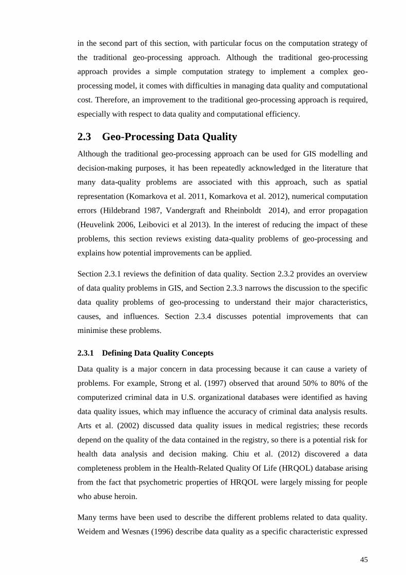
45
in the second part of this section, with particular focus on the computation strategy of
the traditional geo-processing approach. Although the traditional geo-processing
approach provides a simple computation strategy to implement a complex geo-
processing model, it comes with difficulties in managing data quality and computational
cost. Therefore, an improvement to the traditional geo-processing approach is required,
especially with respect to data quality and computational efficiency.
2.3 Geo-Processing Data Quality
Although the traditional geo-processing approach can be used for GIS modelling and
decision-making purposes, it has been repeatedly acknowledged in the literature that
many data-quality problems are associated with this approach, such as spatial
representation (Komarkova et al. 2011, Komarkova et al. 2012), numerical computation
errors (Hildebrand 1987, Vandergraft and Rheinboldt 2014), and error propagation
(Heuvelink 2006, Leibovici et al 2013). In the interest of reducing the impact of these
problems, this section reviews existing data-quality problems of geo-processing and
explains how potential improvements can be applied.
Section 2.3.1 reviews the definition of data quality. Section 2.3.2 provides an overview
of data quality problems in GIS, and Section 2.3.3 narrows the discussion to the specific
data quality problems of geo-processing to understand their major characteristics,
causes, and influences. Section 2.3.4 discusses potential improvements that can
minimise these problems.
2.3.1 Defining Data Quality Concepts
Data quality is a major concern in data processing because it can cause a variety of
problems. For example, Strong et al. (1997) observed that around 50% to 80% of the
computerized criminal data in U.S. organizational databases were identified as having
data quality issues, which may influence the accuracy of criminal data analysis results.
Arts et al. (2002) discussed data quality issues in medical registries; these records
depend on the quality of the data contained in the registry, so there is a potential risk for
health data analysis and decision making. Chiu et al. (2012) discovered a data
completeness problem in the Health-Related Quality Of Life (HRQOL) database arising
from the fact that psychometric properties of HRQOL were largely missing for people
who abuse heroin.
Many terms have been used to describe the different problems related to data quality.
Weidem and Wesnæs (1996) describe data quality as a specific characteristic expressed
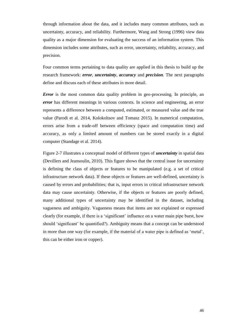
46
through information about the data, and it includes many common attributes, such as
uncertainty, accuracy, and reliability. Furthermore, Wang and Strong (1996) view data
quality as a major dimension for evaluating the success of an information system. This
dimension includes some attributes, such as error, uncertainty, reliability, accuracy, and
precision.
Four common terms pertaining to data quality are applied in this thesis to build up the
research framework: error, uncertainty, accuracy and precision. The next paragraphs
define and discuss each of these attributes in more detail.
Error is the most common data quality problem in geo-processing. In principle, an
error has different meanings in various contexts. In science and engineering, an error
represents a difference between a computed, estimated, or measured value and the true
value (Parodi et al. 2014, Kolokoltsov and Tomasz 2015). In numerical computation,
errors arise from a trade-off between efficiency (space and computation time) and
accuracy, as only a limited amount of numbers can be stored exactly in a digital
computer (Standage et al. 2014).
Figure 2-7 illustrates a conceptual model of different types of uncertainty in spatial data
(Devillers and Jeansoulin, 2010). This figure shows that the central issue for uncertainty
is defining the class of objects or features to be manipulated (e.g. a set of critical
infrastructure network data). If these objects or features are well-defined, uncertainty is
caused by errors and probabilities; that is, input errors in critical infrastructure network
data may cause uncertainty. Otherwise, if the objects or features are poorly defined,
many additional types of uncertainty may be identified in the dataset, including
vagueness and ambiguity. Vagueness means that items are not explained or expressed
clearly (for example, if there is a ‘significant’ influence on a water main pipe burst, how
should ‘significant’ be quantified?). Ambiguity means that a concept can be understood
in more than one way (for example, if the material of a water pipe is defined as ‘metal’,
this can be either iron or copper).
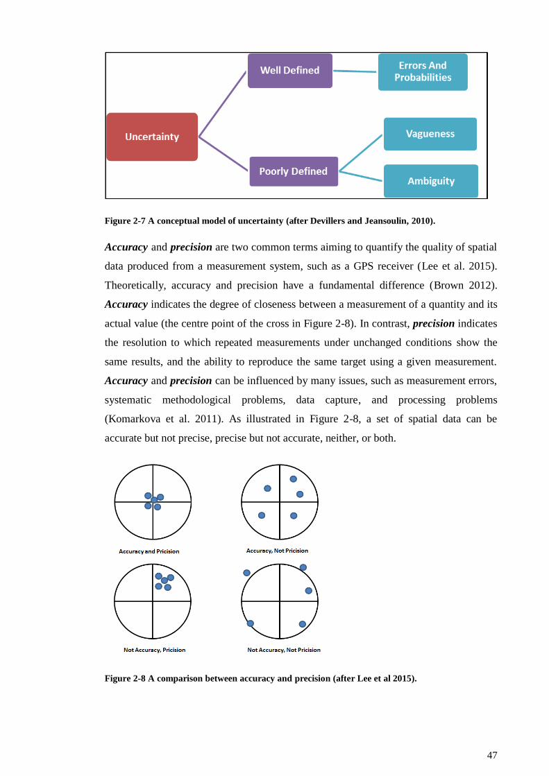
47
Figure 2-7 A conceptual model of uncertainty (after Devillers and Jeansoulin, 2010).
Accuracy and precision are two common terms aiming to quantify the quality of spatial
data produced from a measurement system, such as a GPS receiver (Lee et al. 2015).
Theoretically, accuracy and precision have a fundamental difference (Brown 2012).
Accuracy indicates the degree of closeness between a measurement of a quantity and its
actual value (the centre point of the cross in Figure 2-8). In contrast, precision indicates
the resolution to which repeated measurements under unchanged conditions show the
same results, and the ability to reproduce the same target using a given measurement.
Accuracy and precision can be influenced by many issues, such as measurement errors,
systematic methodological problems, data capture, and processing problems
(Komarkova et al. 2011). As illustrated in Figure 2-8, a set of spatial data can be
accurate but not precise, precise but not accurate, neither, or both.
Figure 2-8 A comparison between accuracy and precision (after Lee et al 2015).
48
Common terms related to data quality can avoid ambiguity in this thesis and enable us
to describe the corresponding data quality problems in detail. Section 2.3.2 provides an
overview of the data quality problems in GIS to help us explore typical data quality
problems in geo-processing.
2.3.2 Overview of Data Quality Problems in GIS
Data quality is a key issue in data processing, as it frequently influences operations,
decision making, and planning. In GIS, the term spatial data quality refers to the degree
of spatial data excellency that satisfies the given conditions and objectives, such as
positional and attribute accuracy (Li et al. 2012). Komarkova et al. (2012) claim that a
higher quality of data and/or information provided by information systems could
support better decision making. However, as spatial data are mainly produced from
models which are simplified from a complex reality, these data have different levels of
imprecise, inaccurate, incomplete, and outdated problems (Devillers and Jeansoulin,
2010).
In order to understand the problems of spatial data quality, Figure 2-9 summarises
typical errors in GIS, including three levels (Beard 1989). The first and most basic level
is the so-called source of errors (Figure 2-9, bottom of the pyramid), which involves
problems that are mainly observed at the stages of data collection, data processing, and
data usage. Data collection errors include errors from field surveys and measurements,
inaccurate equipment and devices, and fuzzy input data. Data processing can lead to
digitising errors, inaccurate prediction and assumption, errors in re-sampling, and error
propagation. Data usage can produce errors due to the misunderstanding of spatial
information.
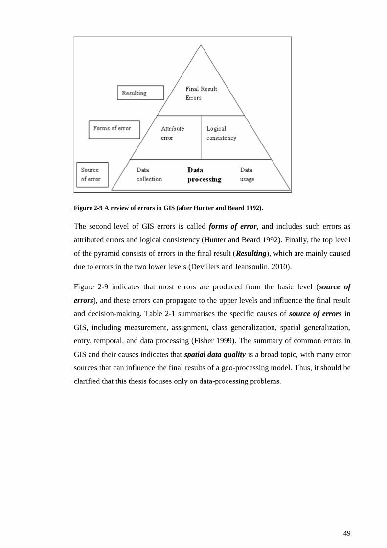
49
Figure 2-9 A review of errors in GIS (after Hunter and Beard 1992).
The second level of GIS errors is called forms of error, and includes such errors as
attributed errors and logical consistency (Hunter and Beard 1992). Finally, the top level
of the pyramid consists of errors in the final result (Resulting), which are mainly caused
due to errors in the two lower levels (Devillers and Jeansoulin, 2010).
Figure 2-9 indicates that most errors are produced from the basic level (source of
errors), and these errors can propagate to the upper levels and influence the final result
and decision-making. Table 2-1 summarises the specific causes of source of errors in
GIS, including measurement, assignment, class generalization, spatial generalization,
entry, temporal, and data processing (Fisher 1999). The summary of common errors in
GIS and their causes indicates that spatial data quality is a broad topic, with many error
sources that can influence the final results of a geo-processing model. Thus, it should be
clarified that this thesis focuses only on data-processing problems.
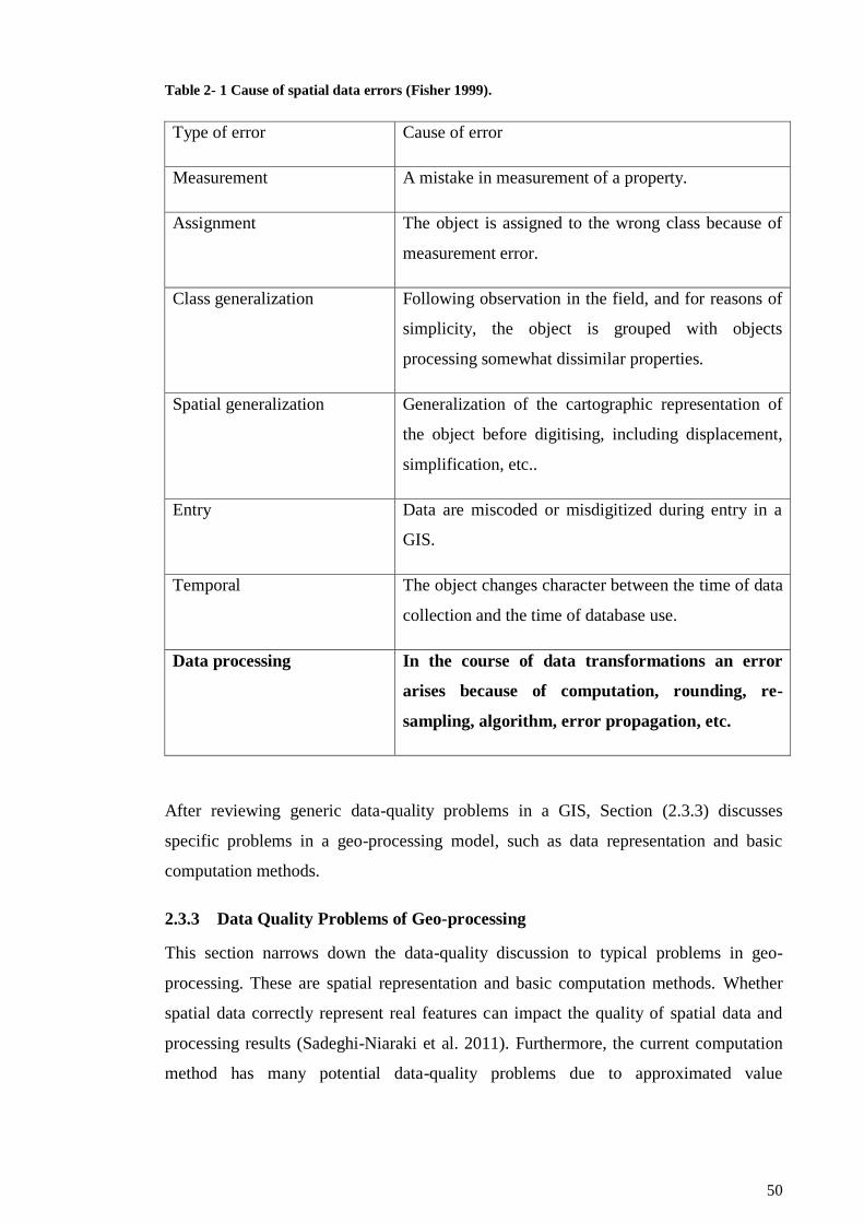
50
Table 2- 1 Cause of spatial data errors (Fisher 1999).
Type of error Cause of error
Measurement A mistake in measurement of a property.
Assignment The object is assigned to the wrong class because of
measurement error.
Class generalization Following observation in the field, and for reasons of
simplicity, the object is grouped with objects
processing somewhat dissimilar properties.
Spatial generalization Generalization of the cartographic representation of
the object before digitising, including displacement,
simplification, etc..
Entry Data are miscoded or misdigitized during entry in a
GIS.
Temporal The object changes character between the time of data
collection and the time of database use.
Data processing In the course of data transformations an error
arises because of computation, rounding, re-
sampling, algorithm, error propagation, etc.
After reviewing generic data-quality problems in a GIS, Section (2.3.3) discusses
specific problems in a geo-processing model, such as data representation and basic
computation methods.
2.3.3 Data Quality Problems of Geo-processing
This section narrows down the data-quality discussion to typical problems in geo-
processing. These are spatial representation and basic computation methods. Whether
spatial data correctly represent real features can impact the quality of spatial data and
processing results (Sadeghi-Niaraki et al. 2011). Furthermore, the current computation
method has many potential data-quality problems due to approximated value
51
(Hildebrand 1987) and error propagation (Rasouli and Timmermans 2013). Hence, this
section discusses spatial representation and basic computation methods in detail.
2.3.3.1 Spatial Representation
A fundamental issue in geo-processing is how spatial features can be represented in a
digital environment to produce meaningful information (Komarkova et al. 2011,
Komarkova et al. 2012). Many spatial data models are used for storing geographical
data digitally, while others have been proposed for different purposes, such as
describing discrete objects and continuous field features.
Vector data comprise the most common spatial data model for describing discrete
objects, and can be used to store linear features, such as city locations, popular places,
road networks, and national boundaries, on a digital computer (Worboys and Duckham,
2004). There are three main advantages of vector data. First, vector data offer an
accurate spatial representation of spatial objects at all levels (Worboys and Duckham,
2004). For example, spatial objects may be represented at their original resolution,
without map generalisation, and maintained by location. Secondly, vector data provide
an easy way to retrieve, update, and generalise spatial attributes. For instance, the
attributes of a point, including its coordinate value and location name, can be directly
modified or updated by users. Lastly, more complicated spatial features, such as
topological networks, can be represented and described explicitly and efficiently using
vector data (Dowers et al. 2000).
Compared with vector data, raster data can be used to effectively describe continuous
field features. In principle, raster data divide the real-world surface into an array or
matrix of pixels in a continuous field, and each pixel represents its position and attribute
in a raster layer (Worboys and Duckham, 2004). In fact, raster data provide an easier
and faster way to describe continuous surfaces. There are three advantages of raster data
for representing continuous fields. First, raster data have a simplified data structure (e.g.
a matrix of cell values) and thus can be more easily processed by computer
programming tools (Worboys and Duckham, 2004). Secondly, raster data provide an
efficient way to model continuous data and perform surface analysis. Thirdly, raster
data are ideally suited for GIS functions such as query and overlay, as a pixel size can
be converted to a specific dimension using interpolation methods (Arbia et al.1998).
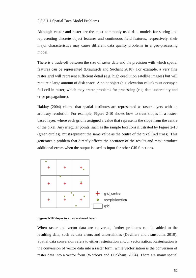
52
2.3.3.1.1 Spatial Data Model Problems
Although vector and raster are the most commonly used data models for storing and
representing discrete object features and continuous field features, respectively, their
major characteristics may cause different data quality problems in a geo-processing
model.
There is a trade-off between the size of raster data and the precision with which spatial
features can be represented (Braunisch and Suchant 2010). For example, a very fine
raster grid will represent sufficient detail (e.g. high-resolution satellite images) but will
require a large amount of disk space. A point object (e.g. elevation value) must occupy a
full cell in raster, which may create problems for processing (e.g. data uncertainty and
error propagations).
Haklay (2004) claims that spatial attributes are represented as raster layers with an
arbitrary resolution. For example, Figure 2-10 shows how to treat slopes in a raster-
based layer, where each grid is assigned a value that represents the slope from the centre
of the pixel. Any irregular points, such as the sample locations illustrated by Figure 2-10
(green circles), must represent the same value as the centre of the pixel (red cross). This
generates a problem that directly affects the accuracy of the results and may introduce
additional errors when the output is used as input for other GIS functions.
Figure 2-10 Slopes in a raster-based layer.
When raster and vector data are converted, further problems can be added to the
resulting data, such as data errors and uncertainties (Devillers and Jeansoulin, 2010).
Spatial data conversion refers to either rasterisation and/or vectorisation. Rasterisation is
the conversion of vector data into a raster form, while vectorisation is the conversion of
raster data into a vector form (Worboys and Duckham, 2004). There are many spatial
53
data-quality problems associated with rasterisation and vectorisation functions.
Rasterisation involves a loss of information, such as topological relationships, which
may lead to missing data and produce data uncertainties in the spatial analysis
(Dendoncker et al. 2008). In vectorisation, two choices are possible for converting the
raster into a vector data model: either no more information is added, and the result may
have significant pixel edges, or additional data are needed to smooth pixel borders, but
no accurate information is available (Kovalerchuk and Perlovsky 2011).
This section discusses the major GIS representation problems in the traditional geo-
processing approach. Section (2.3.3.2) discusses the computation method for geo-
processing to understand how errors and data uncertainties are produced and propagated
in the traditional geo-processing approach.
2.3.3.2 Geo-processing Computation
A computation is a process that manipulates one or more input in order to produce one
or more results. In GIS, computations are used to interpret spatial characteristics,
explain geographical phenomena, and solve spatial problems (Couclelis 1998; Cheng et
al. 2012). This section discusses the drawbacks of computation methods in the
traditional geo-processing approach.
2.3.3.2.1 Numerical Computation Problems
Numerical computation is widely used by current GIS software packages (e.g. ArcGIS,
MapInfo, GRASS, and Manifold) for data recording and storage purposes. Numerical
computation uses numerical approximation algorithms to represent mathematical
equations, which are usually expressed using algebra, differentiation, integration, or
other types of equations. The problem with numerical computation is that, because
digital computers cannot accurately express real numbers, all results obtained using
numerical calculations approximate the true value (Hoffmann 1989).
Hildebrand (1987) defined the relationship between an approximation and its true value
using Formula 2.1, in which the true value is the real value without any distortions and
errors, and the approximation is the result of numerical computations. This equation
indicates that errors always accompany approximated values.
True value = approximation + error (Formula 2.1)
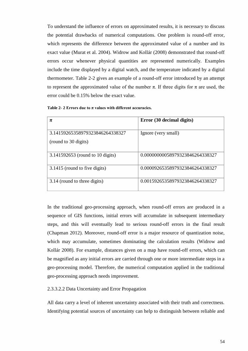
54
To understand the influence of errors on approximated results, it is necessary to discuss
the potential drawbacks of numerical computations. One problem is round-off error,
which represents the difference between the approximated value of a number and its
exact value (Murat et al. 2004). Widrow and Kollár (2008) demonstrated that round-off
errors occur whenever physical quantities are represented numerically. Examples
include the time displayed by a digital watch, and the temperature indicated by a digital
thermometer. Table 2-2 gives an example of a round-off error introduced by an attempt
to represent the approximated value of the number π. If three digits for π are used, the
error could be 0.15% below the exact value.
Table 2- 2 Errors due to π values with different accuracies.
In the traditional geo-processing approach, when round-off errors are produced in a
sequence of GIS functions, initial errors will accumulate in subsequent intermediary
steps, and this will eventually lead to serious round-off errors in the final result
(Chapman 2012). Moreover, round-off error is a major resource of quantization noise,
which may accumulate, sometimes dominating the calculation results (Widrow and
Kollár 2008). For example, distances given on a map have round-off errors, which can
be magnified as any initial errors are carried through one or more intermediate steps in a
geo-processing model. Therefore, the numerical computation applied in the traditional
geo-processing approach needs improvement.
2.3.3.2.2 Data Uncertainty and Error Propagation
All data carry a level of inherent uncertainty associated with their truth and correctness.
Identifying potential sources of uncertainty can help to distinguish between reliable and
π Error (30 decimal digits)
3.14159265358979323846264338327
(round to 30 digits)
Ignore (very small)
3.141592653 (round to 10 digits) 0.00000000058979323846264338327
3.1415 (round to five digits) 0.00009265358979323846264338327
3.14 (round to three digits) 0.00159265358979323846264338327
55
unreliable data. Most data uncertainty is associated with errors in direct measurements
of a quantity (Morgan et al. 1990).
Within a GIS, no spatial data are truly error-free, because much of the data are produced
by assumption, interpolation, and prediction methods (Devillers and Jeansoulin 2010).
An assumption is a major resource of data uncertainty because it provides something
that users assume to be true or assume will happen, often without proof. As Shahriar et
al. (2012) discuss, it is a challenge to characterise model uncertainty that arises from an
assumption of independence among different risk events. Interpolation is another major
resource of data uncertainty, as it produces data based on a assumed value. Brodlie et al.
(2012) claim that uncertainty is introduced in an interpolation step by guessing the
output data. Additionally, a prediction or forecast could increase the chances of data
uncertainties because it deals with the future. For example, a weather forecast is an
application of science and technology to predict information (e.g. temperature, wind
speed) about the atmosphere in a specific location, but these data have multiple
uncertainties due to interpolations (Hu et al. 2010).
When users select spatial data from a GIS database to use as input datasets for a geo-
processing process, errors and uncertainties that exist in the input data will propagate to
the output of the function (Bingham and Karssenberg 2014). Error propagation becomes
more complicated when the output from one function or a sub-model is used as the
input for a subsequent function or sub-model (Rasouli and Timmermans 2013). For
example, re-sampling is an important function in image processing, as it can be used for
the integration of different raster layers (Skifi and Bosner 2014); however, the re-
sampling process complicates the raster overlay function and introduces uncertainties
into the computations, and is a major source of error propagation (Haklay, 2004).
Moreover, inaccuracies (e.g. data errors and data uncertainties) may be introduced
during this calculation step, which will also affect any subsequent computations due to
error propagation.
This section discussed the major data quality problems of geo-processing. The
drawbacks of spatial representation and computation methods applied in the traditional
geo-processing approach can cause many data quality problems and influence the final
results. The next section discusses how these data-quality problems could be improved
using the new CG approach.
56
2.3.4 Data Quality Improvement
The problems discussed in Section 2.3.3 lead us to the conclusion that we need to
address data-quality concerns in traditional geo-processing. Nevertheless, it is widely
accepted that data uncertainty and its related implications cannot be avoided, but rather
can be managed (He et al. 2004, Heuvelink 2006).
The CG approach is proposed in this thesis with the aim to improve the data quality and
computational efficiency of geo-processing. Specifically, a set of methods comprising
the CG approach, including a point-based spatial data model, symbolic computation,
and functional layers, is introduced to address the previously discussed problems.
2.3.4.1 Spatial Data Model Improvement
It was noted that raster and vector data are popular spatial data models to represent the
real world features. However, these two spatial data models introduce data quality
problems into geo-processing, such as the resolution of raster data and conversion
between raster data and vector data. This section reviews other spatial data
representation method in order to provide a suggestion for reducing the influence of
raster and vector data in the traditional geo-processing approach.
2.3.4.1.1 Spatial Data Models Review
This section discusses how spatial features can be described using different
representation methods. These is a Triangulated Irregular Network (TIN).
A TIN is a vector-based spatial data model used to represent elevation in a 3D surface
(Worboys and Duckham, 2004), and is comprised of triangles which are constructed
from a set of points with ‘X and Y’ coordinate values and ‘Z’ elevation values.
Moreover, each triangle apart from the coordinates is further associated with topological
information. As Longley et al. (2005) explain, the key benefit of a TIN is that the
density of sampled points, and consequently the size of triangles, can be adjusted to
better reflect the relief of the surface that it is being modelled. In contrast to raster data
(e.g. DEM), an advantage of TINs is that points are distributed based on the complexity
of an area (De Smith et al. 2007). Therefore, TIN data are flexible and require less
storage space, especially when compared with raster data models. However, a
disadvantage of TIN data is that they can be hard or extremely complex to integrate
with other spatial data models.
57
2.3.4.1.2 Point-based Spatial Data Model
Point data play an important role in spatial representation, as the majority of spatial data
models are based on, or consist of, points. For example, as Table 2-3 demonstrates, a
polygon (vector data) is composed of a group of points, and a raster image (raster data)
is constructed from a matrix of values or centroids with grid size. Additionally, a 3D
object can be represented using point data (e.g. X, Y coordinates and Z elevation value)
(Chen and Schneider 2009). Table 2-3 illustrates that the point-based spatial model has
more flexibility for representing various spatial objects. For example, when point-based
spatial data are processed in a model, the outputs can take any form of spatial data
model (e.g. raster or vector) according to the user’s request.
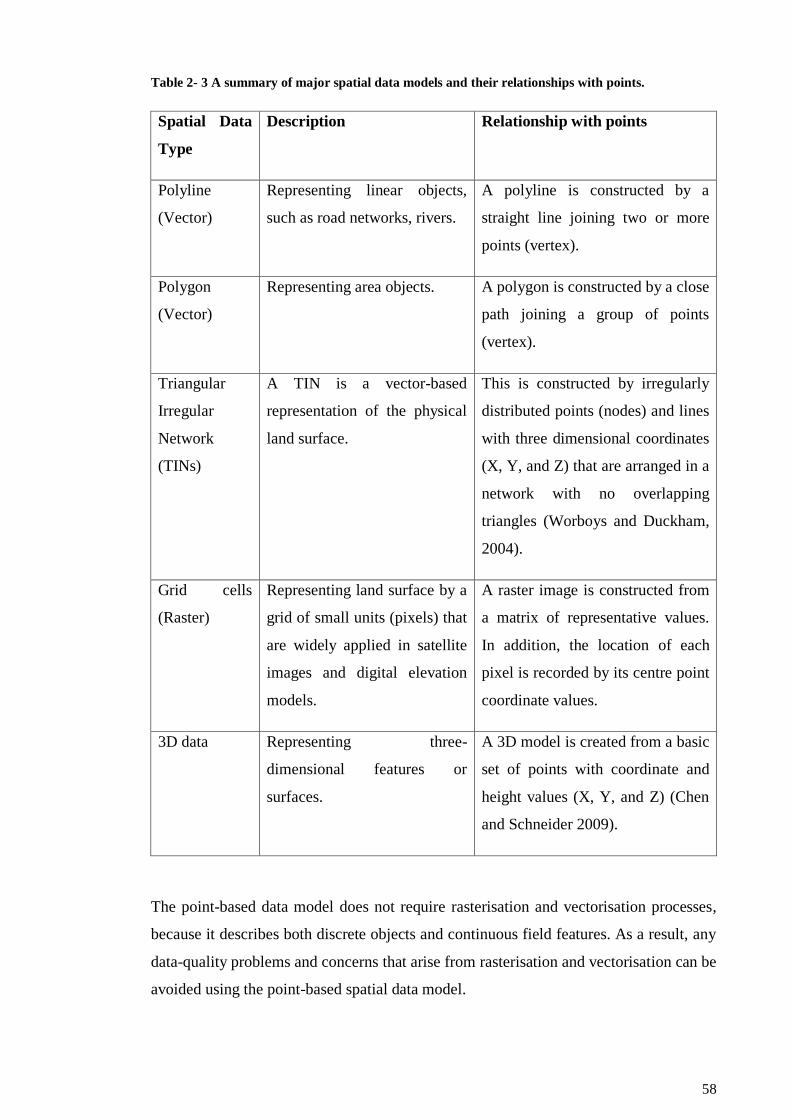
58
Table 2- 3 A summary of major spatial data models and their relationships with points.
Spatial Data
Type
Description Relationship with points
Polyline
(Vector)
Representing linear objects,
such as road networks, rivers.
A polyline is constructed by a
straight line joining two or more
points (vertex).
Polygon
(Vector)
Representing area objects.
A polygon is constructed by a close
path joining a group of points
(vertex).
Triangular
Irregular
Network
(TINs)
A TIN is a vector-based
representation of the physical
land surface.
This is constructed by irregularly
distributed points (nodes) and lines
with three dimensional coordinates
(X, Y, and Z) that are arranged in a
network with no overlapping
triangles (Worboys and Duckham,
2004).
Grid cells
(Raster)
Representing land surface by a
grid of small units (pixels) that
are widely applied in satellite
images and digital elevation
models.
A raster image is constructed from
a matrix of representative values.
In addition, the location of each
pixel is recorded by its centre point
coordinate values.
3D data Representing three-
dimensional features or
surfaces.
A 3D model is created from a basic
set of points with coordinate and
height values (X, Y, and Z) (Chen
and Schneider 2009).
The point-based data model does not require rasterisation and vectorisation processes,
because it describes both discrete objects and continuous field features. As a result, any
data-quality problems and concerns that arise from rasterisation and vectorisation can be
avoided using the point-based spatial data model.
59
Additionally, the point-based spatial data model provides a way to reduce the
complexity of spatial data models (Jjumba and Dragicevic 2014, Camara et al. 2014).
Although many types of spatial models have been created to model spatial features,
such as vector, raster, TIN, and 3D data, these structures directly increase the
complexity of a GIS database, and this complexity may potentially increase the
difficulty of maintaining the realism and clarity of the system content (Goodchild et al.
2007).
For these reasons, the point-based spatial data model is introduced in the CG approach
to improve its spatial representation.
2.3.4.2 Geo-processing Computation Improvement
It was discussed that numerical computation and sequential computation are applied in
the traditional geo-processing approach for spatial data calculation. However, there are
some data quality problems in these methods, such as approximate values and error
propagation. This section explains the reasoning behind using symbolic computation
and function-based layers in the CG approach to improve the data quality of geo-
processing.
2.3.4.2.1 Symbolic Computation and Function-Based Layer
An alternative to the numerical computation applied in the traditional geo-processing
approach is symbolic computation. Symbolic computation provides an exact method of
mathematical calculation, such as differentiation and integration, linear algebra and
matrix calculus, and the simplification of algebraic equations (Grossman 1989). A
significant characteristic of symbolic computation is that mathematical formulas are
manipulated in a symbolic form. Heck (2003) noted that symbols can represent numbers
such as integers, rational numbers, real numbers and complex numbers, but they may
also be used to represent mathematical operations.
Symbolic calculation provides greater flexibility for users to define the quality of a
result (Carminati and Vu 2000). Software applications that perform symbolic
calculations are called computer algebra systems (Cafuta et al. 2011). Such systems
have been widely used in various applications, such as high energy physics, chemical
engineering, mechanics, cybernetics, and computer science.
Symbolic computation has two main advantages for mathematical computations in a
geo-processing model (Hoffmann 1989). First, it could avoid a large number of
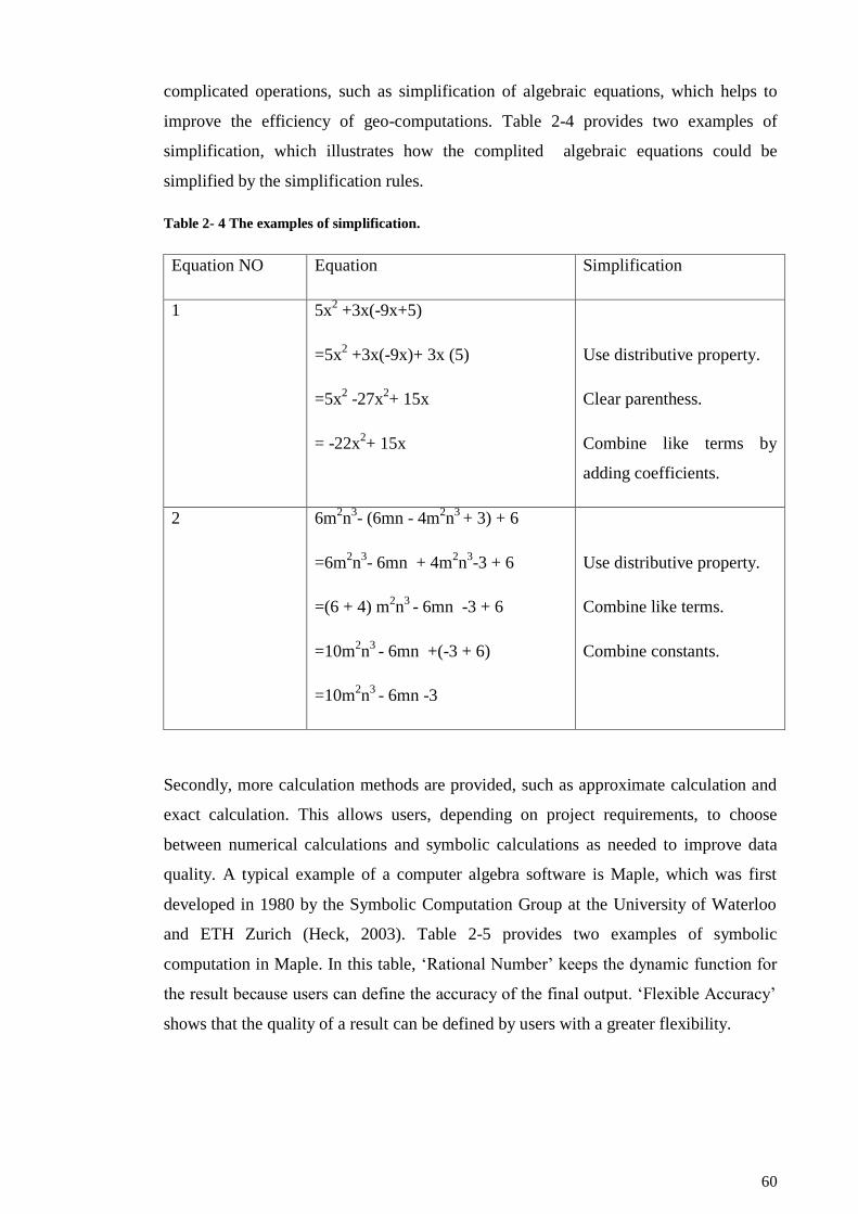
60
complicated operations, such as simplification of algebraic equations, which helps to
improve the efficiency of geo-computations. Table 2-4 provides two examples of
simplification, which illustrates how the complited algebraic equations could be
simplified by the simplification rules.
Table 2- 4 The examples of simplification.
Equation NO Equation Simplification
1 5x2 +3x(-9x+5)
=5x2 +3x(-9x)+ 3x (5)
=5x2 -27x
2+ 15x
= -22x2+ 15x
Use distributive property.
Clear parenthess.
Combine like terms by
adding coefficients.
2 6m2n
3- (6mn - 4m
2n
3 + 3) + 6
=6m2n
3- 6mn + 4m
2n
3-3 + 6
=(6 + 4) m2n
3 - 6mn -3 + 6
=10m2n
3 - 6mn +(-3 + 6)
=10m2n
3 - 6mn -3
Use distributive property.
Combine like terms.
Combine constants.
Secondly, more calculation methods are provided, such as approximate calculation and
exact calculation. This allows users, depending on project requirements, to choose
between numerical calculations and symbolic calculations as needed to improve data
quality. A typical example of a computer algebra software is Maple, which was first
developed in 1980 by the Symbolic Computation Group at the University of Waterloo
and ETH Zurich (Heck, 2003). Table 2-5 provides two examples of symbolic
computation in Maple. In this table, ‘Rational Number’ keeps the dynamic function for
the result because users can define the accuracy of the final output. ‘Flexible Accuracy’
shows that the quality of a result can be defined by users with a greater flexibility.
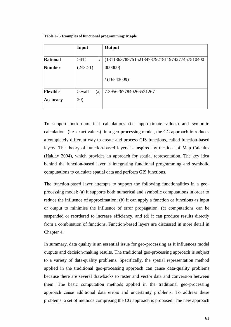
61
Table 2- 5 Examples of functional programming: Maple.
Input Output
Rational
Number
>41! /
(2^32-1)
(131186378875152184737921811974277457510400
000000)
/ (16843009)
Flexible
Accuracy
>evalf (a,
20)
7.39562677840266521267
To support both numerical calculations (i.e. approximate values) and symbolic
calculations (i.e. exact values) in a geo-processing model, the CG approach introduces
a completely different way to create and process GIS functions, called function-based
layers. The theory of function-based layers is inspired by the idea of Map Calculus
(Haklay 2004), which provides an approach for spatial representation. The key idea
behind the function-based layer is integrating functional programming and symbolic
computations to calculate spatial data and perform GIS functions.
The function-based layer attempts to support the following functionalities in a geo-
processing model: (a) it supports both numerical and symbolic computations in order to
reduce the influence of approximation; (b) it can apply a function or functions as input
or output to minimise the influence of error propagation; (c) computations can be
suspended or reordered to increase efficiency, and (d) it can produce results directly
from a combination of functions. Function-based layers are discussed in more detail in
Chapter 4.
In summary, data quality is an essential issue for geo-processing as it influences model
outputs and decision-making results. The traditional geo-processing approach is subject
to a variety of data-quality problems. Specifically, the spatial representation method
applied in the traditional geo-processing approach can cause data-quality problems
because there are several drawbacks to raster and vector data and conversion between
them. The basic computation methods applied in the traditional geo-processing
approach cause additional data errors and uncertainty problems. To address these
problems, a set of methods comprising the CG approach is proposed. The new approach

62
includes a point-based spatial data model, a symbolic computation, and a function-based
layer. The point-based spatial data model minimises spatial representation problems,
while symbolic computation and function-based layers reduce data error and uncertainty
when users apply numerical computation in a geo-processing model.
2.4 Computational Efficiency of Geo-Processing
The sequential computation strategy applied in the traditional geo-processing approach
not only has data-quality problems, but also causes computational efficiency problems
such as extra computation time costs. Consequently, problems related to computational
efficiency need to be further considered in this thesis.
This section continues to discuss the problems of the traditional geo-processing
approach, toward the aim of improving the computational efficiency of geo-processing.
Section 2.4.1 reviews computational efficiency concepts and Section 2.4.2 discusses
computational efficiency problems associated with the traditional geo-processing
approach. Section 2.4.3 discusses how computational efficiency in geo-processing can
be improved using the CG approach.
2.4.1 Defining the Computational Efficiency Concept
Computational efficiency is a common term used in digital computation to quantify the
performance of a digital device. For example, computational efficiency can refer to the
resources (e.g. computer memory and computation time) used by an algorithm (Liu and
Wang 2012). ‘Big O’ notation is used to quantify the performance of algorithms (e.g.
processing time or working space requirements) when they have different input data
(Cormen et al. 2001; De Smith et al. 2007). As illustrated in Figure 2-11, denotes
processing time or memory space that is constant (a flat line) regardless of the size of
the dataset; indicates linear growth in direct proportion to the size of the input
dataset, that means the performance is directly dependent on the size of the input data;
and indicate the performance will be directly proportional to a
power of the input data size; and and denote growth curves that rise
sharply at the beginning of the execution and then increase more slowly as the size of
the dataset grows.
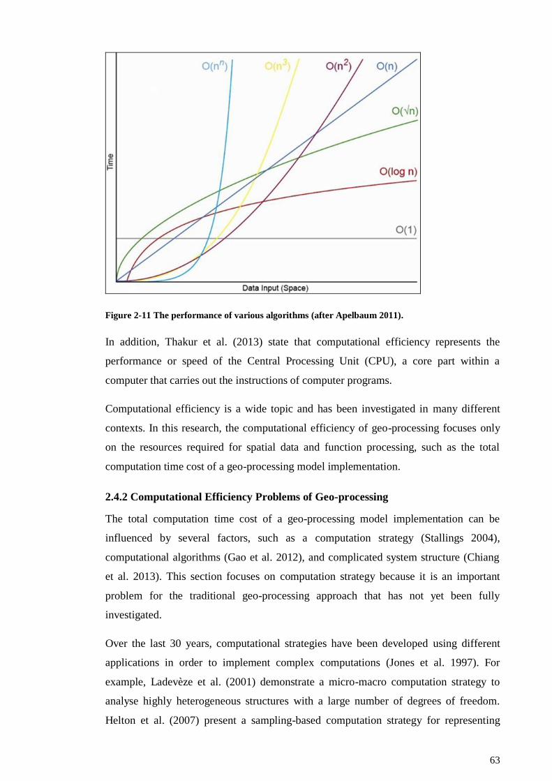
63
Figure 2-11 The performance of various algorithms (after Apelbaum 2011).
In addition, Thakur et al. (2013) state that computational efficiency represents the
performance or speed of the Central Processing Unit (CPU), a core part within a
computer that carries out the instructions of computer programs.
Computational efficiency is a wide topic and has been investigated in many different
contexts. In this research, the computational efficiency of geo-processing focuses only
on the resources required for spatial data and function processing, such as the total
computation time cost of a geo-processing model implementation.
2.4.2 Computational Efficiency Problems of Geo-processing
The total computation time cost of a geo-processing model implementation can be
influenced by several factors, such as a computation strategy (Stallings 2004),
computational algorithms (Gao et al. 2012), and complicated system structure (Chiang
et al. 2013). This section focuses on computation strategy because it is an important
problem for the traditional geo-processing approach that has not yet been fully
investigated.
Over the last 30 years, computational strategies have been developed using different
applications in order to implement complex computations (Jones et al. 1997). For
example, Ladevèze et al. (2001) demonstrate a micro-macro computation strategy to
analyse highly heterogeneous structures with a large number of degrees of freedom.
Helton et al. (2007) present a sampling-based computation strategy for representing
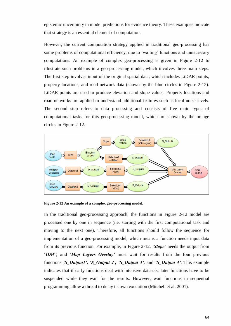
64
epistemic uncertainty in model predictions for evidence theory. These examples indicate
that strategy is an essential element of computation.
However, the current computation strategy applied in traditional geo-processing has
some problems of computational efficiency, due to ‘waiting’ functions and unnecessary
computations. An example of complex geo-processing is given in Figure 2-12 to
illustrate such problems in a geo-processing model, which involves three main steps.
The first step involves input of the original spatial data, which includes LiDAR points,
property locations, and road network data (shown by the blue circles in Figure 2-12).
LiDAR points are used to produce elevation and slope values. Property locations and
road networks are applied to understand additional features such as local noise levels.
The second step refers to data processing and consists of five main types of
computational tasks for this geo-processing model, which are shown by the orange
circles in Figure 2-12.
Figure 2-12 An example of a complex geo-processing model.
In the traditional geo-processing approach, the functions in Figure 2-12 model are
processed one by one in sequence (i.e. starting with the first computational task and
moving to the next one). Therefore, all functions should follow the sequence for
implementation of a geo-processing model, which means a function needs input data
from its previous function. For example, in Figure 2-12, ‘Slope’ needs the output from
‘IDW’, and ‘Map Layers Overlay’ must wait for results from the four previous
functions ‘S_Output1’, ‘S_Output 2’, ‘S_Output 3’, and ‘S_Output 4’. This example
indicates that if early functions deal with intensive datasets, later functions have to be
suspended while they wait for the results. However, wait functions in sequential
programming allow a thread to delay its own execution (Mitchell et al. 2001).
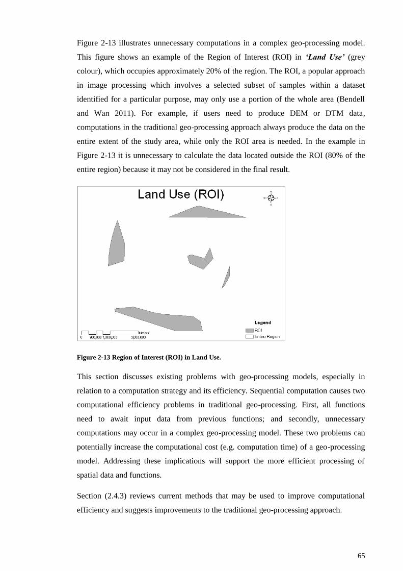
65
Figure 2-13 illustrates unnecessary computations in a complex geo-processing model.
This figure shows an example of the Region of Interest (ROI) in ‘Land Use’ (grey
colour), which occupies approximately 20% of the region. The ROI, a popular approach
in image processing which involves a selected subset of samples within a dataset
identified for a particular purpose, may only use a portion of the whole area (Bendell
and Wan 2011). For example, if users need to produce DEM or DTM data,
computations in the traditional geo-processing approach always produce the data on the
entire extent of the study area, while only the ROI area is needed. In the example in
Figure 2-13 it is unnecessary to calculate the data located outside the ROI (80% of the
entire region) because it may not be considered in the final result.
Figure 2-13 Region of Interest (ROI) in Land Use.
This section discusses existing problems with geo-processing models, especially in
relation to a computation strategy and its efficiency. Sequential computation causes two
computational efficiency problems in traditional geo-processing. First, all functions
need to await input data from previous functions; and secondly, unnecessary
computations may occur in a complex geo-processing model. These two problems can
potentially increase the computational cost (e.g. computation time) of a geo-processing
model. Addressing these implications will support the more efficient processing of
spatial data and functions.
Section (2.4.3) reviews current methods that may be used to improve computational
efficiency and suggests improvements to the traditional geo-processing approach.
66
2.4.3 Computational Efficiency Improvement
In geo-processing, issues related to computational efficiency have received increasing
attention due to the number and complexity of spatial problems, which have both
increased dramatically in recent years. This section reviews recent computational
methods to facilitate a later demonstration of how computational efficiency problems in
traditional geo-processing can be addressed.
2.4.3.1 Modern Computation Methods Review
In recent years, many high performance computational techniques have been applied in
GIS to improve computational efficiency, including parallel computation and spatial
data query methods. Parallel computation has been widely used in GIS as it enables the
implementation of multiple instructions by using multi-core processors (Grama 2003).
Spatial query is a fundamental function which supports various spatial analyses and data
processing applications (Zhong et al. 2012). These two methods are discussed in the
next Sections (2.4.3.1.1 and 2.4.3.1.2).
2.4.3.1.1 Parallel Computation
Before 2005, most CPUs had only one core for processing all instructions, which
frequently influenced the computational efficiency as the instructions had to be
implemented one by one. Then, the multi-core processor (including more than one core
in a single computing component) was introduced in 2009. The multi-core processor
supported a way to run multiple instructions at the same time and increase overall speed
for programs amenable to parallel computation.
In traditional computing, a problem is divided into a discrete series of instructions
which are executed sequentially on a single processor. In contrast, parallel computation
breaks a problem into discrete parts, with each part further divided into a series of
instructions. Final instructions for each part execute concurrently on a multi-core
processor or different processors (Megiddo 1983).
Currently, parallel computation is widely used in GIS in order to improve computational
efficiency, especially in relation to large data sharing, dynamic data processing, and
web-GIS. Jiang et al. (2012) proposed a parallel computation approach of spatial vector
data conversion based on a common interface, which provides an efficient way to share
large geospatial data from a variety of data resources. Kremmydas et al. (2011)
developed a parallel computation approach to reduce the data processing time of a web
67
based Spatial Decision Support System (web SDSS), which was implemented in
Thessaly to evaluate the supply of selected energy crops. These studies showed that
total solution time drops significantly under the parallel computational approach.
Although parallel computation can improve the computational efficiency of traditional
geo-processing by using a multi-core processor, it does not change the sequential
computation strategy. Consequently, the problems discussed in Section 2.4.2 still exist
in parallel computation.
2.4.3.1.2 Spatial Data Query
In addition to parallel computation, many other methods can be used to improve
computational efficiency and performance in geo-processing. For example, spatial data
query methods support a way to access and search larger spatial databases more
efficiently to reduce the entire computation time of a geo-processing model.
Guttman (1984) describes the so-called R tree, a spatial data access method used to
store, search, and query spatial information. The R-tree method is an efficient way to
query a spatial database as it reduces computer memory and temporary database usage.
R-tree has been widely used in different applications of spatial data management. For
example, R-tree is commonly used to store spatial data, such road networks and city
locations, and then to query the data quickly and efficiently; for example, to ‘Find a
shortest distance from city A to city B’ or ‘Find a nearest motorway access point around
city C’. Spatial data query methods are widely used in GIS to improve the
computational speed of access, query, and storage of large spatial databases (Luo et al.
2012, Aji et al. 2012).
Kriegel et al. (1993) discuss a method which combines spatial access and computational
geometry concepts to improve the performance of GIS operations. The method can be
used in different applications or algorithms, such as map overlay and map merge.
However, the current method needs further investigation into the design of efficient
algorithms based on spatial access methods and computational geometry for all retrieval
operations.
To sum up, spatial data query methods contribute to geo-processing, especially with
respect to accessing and querying large spatial datasets. Nevertheless, these methods do
not improve the computational efficiency of executing a large group of computation
tasks in a geo-processing model.
68
2.4.3.2 Computation strategy
Although computational efficiency of geo-processing could be improved using parallel
computational and spatial data query, these methods do not address the sequential
computation problem in the traditional geo-processing approach. This means that spatial
data and functions are still evaluated one by one until the final result is computed in
parallel.
In order to address the sequential computation problem in the traditional geo-processing
approach, this section discusses how a different computation strategy, priority-based
computation, can be used for geo-processing.
Computational priority, or scheduling, is a method that optimizes use of computation
resources and improves computation performance (Jones et al. 1997). In computer
science, priority (or scheduling) is used for implementing multiple computation tasks.
For example, scheduling could be used to suspend a heavy computation task in order to
free up the main computing memory for other computation tasks which have less
computational cost (e.g. time and memory) (Stallings 2004). Moreover, priority (or
scheduling) has also been widely applied in GIS, mainly for the purposes of determining
least-cost paths across a continuous surface (De Smith et al. 2007) or reducing delay
due to an unexpected event in a complex railway network (Pellegrini et al. 2014)
Similar to the priority rule used in computer science or in spatial problems of path
selection, the priority-based computation strategy provides a new computation strategy
in geo-processing to implement various computation tasks more efficiently, especially
by lowering computation time and use of costly computer resources. In the priority-
based computation strategy, priority (or scheduling) can be used to suspend a
computation task that has a low priority, or a computation task which allocates a large
amount of memory, in order to free up main memory for other computation tasks,
implementing the computation task later when more computer memory is available
(Stallings 2004). More details of priority-based computation strategy will be discussed
in Chapter 7.
In summary, computational efficiency is an important concern in geo-processing, as it
can influence computation performance and delay decision-making. In particular, the
current computation strategy (sequential computation) applied in traditional geo-
processing can cost extra computation time and computer memory because it involves
‘waiting’ functions and unnecessary computations. In view of our study of
69
computational efficiency methods, we propose a priority-based computation strategy for
the CG approach in order to improve the computation time of a complex geo-processing
model.
2.5 Conclusion
Geo-processing is used to solve complex spatial problems. The traditional geo-
processing approach has been widely applied in tools for spatial modelling, spatial
analysis, and decision-making systems. Although the traditional geo-processing
approach provides a simplified computation strategy for implementing a complex
spatial model, the trade-off between simplification and complexity shows that data
quality and computational cost have yet to be fully understood in the traditional geo-
processing approach.
Data quality is a key concern in a geo-processing model because it influences the final
geo-processing outputs and decision support system. Our review of data quality under
the traditional geo-processing approach (Section 2.3.3) shows that the current approach
is influenced by several data-quality problems. The first problem is the current spatial
data representation, which may cause problems due to the limitations of raster and
vector data formats. The second problem involves basic computation methods, which
also can cause data error and uncertainty problems due to numeric computation and
error propagation.
Computational efficiency is another important concern for geo-processing, as it can
influence computation performance. Our review of computational efficiency in
traditional geo-processing (Section 2.4.2) suggests that the current computation strategy
(sequential computation) costs extra computation time and computer memory because it
employs inefficient processes (i.e. waiting functions) and unnecessary computations.
This thesis introduces the CG approach in order to address these problems related to
data quality and computational efficiency. A set of methods is proposed for the CG
approach, including a point-based spatial data model, a symbolic computation, a
function-based layer, and a priority-based computation strategy. The point-based spatial
data model is used to minimise spatial data representation problems such as data
conversion. The symbolic computation method and function-based layers are applied to
reduce the data error and uncertainty associated with numerical computation in a geo-
processing model. The priority-based computation strategy is used to reduce
computation time by re-ordering the computational sequence.

70
This chapter has reviewed the current data quality and computational efficiency
problems that arise under the traditional geo-processing approach, and has discussed the
methods that we apply in the CG approach for improvement of these issues. The next
chapter discusses the conceptual model of the CG approach, which provides a basic
element for the development of the new approach.
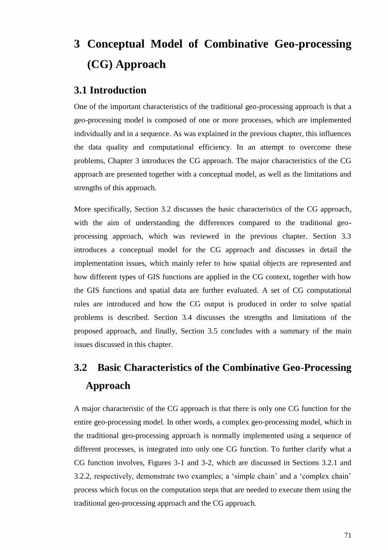
71
3 Conceptual Model of Combinative Geo-processing
(CG) Approach
3.1 Introduction
One of the important characteristics of the traditional geo-processing approach is that a
geo-processing model is composed of one or more processes, which are implemented
individually and in a sequence. As was explained in the previous chapter, this influences
the data quality and computational efficiency. In an attempt to overcome these
problems, Chapter 3 introduces the CG approach. The major characteristics of the CG
approach are presented together with a conceptual model, as well as the limitations and
strengths of this approach.
More specifically, Section 3.2 discusses the basic characteristics of the CG approach,
with the aim of understanding the differences compared to the traditional geo-
processing approach, which was reviewed in the previous chapter. Section 3.3
introduces a conceptual model for the CG approach and discusses in detail the
implementation issues, which mainly refer to how spatial objects are represented and
how different types of GIS functions are applied in the CG context, together with how
the GIS functions and spatial data are further evaluated. A set of CG computational
rules are introduced and how the CG output is produced in order to solve spatial
problems is described. Section 3.4 discusses the strengths and limitations of the
proposed approach, and finally, Section 3.5 concludes with a summary of the main
issues discussed in this chapter.
3.2 Basic Characteristics of the Combinative Geo-Processing
Approach
A major characteristic of the CG approach is that there is only one CG function for the
entire geo-processing model. In other words, a complex geo-processing model, which in
the traditional geo-processing approach is normally implemented using a sequence of
different processes, is integrated into only one CG function. To further clarify what a
CG function involves, Figures 3-1 and 3-2, which are discussed in Sections 3.2.1 and
3.2.2, respectively, demonstrate two examples; a ‘simple chain’ and a ‘complex chain’
process which focus on the computation steps that are needed to execute them using the
traditional geo-processing approach and the CG approach.
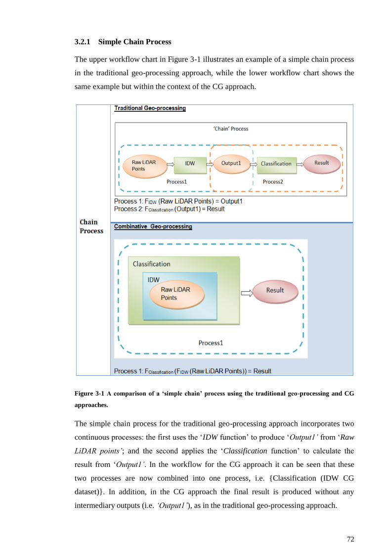
72
3.2.1 Simple Chain Process
The upper workflow chart in Figure 3-1 illustrates an example of a simple chain process
in the traditional geo-processing approach, while the lower workflow chart shows the
same example but within the context of the CG approach.
Figure 3-1 A comparison of a ‘simple chain’ process using the traditional geo-processing and CG
approaches.
The simple chain process for the traditional geo-processing approach incorporates two
continuous processes: the first uses the ‘IDW function’ to produce ‘Output1’ from ‘Raw
LiDAR points’; and the second applies the ‘Classification function’ to calculate the
result from ‘Output1’. In the workflow for the CG approach it can be seen that these
two processes are now combined into one process, i.e. {Classification (IDW CG
dataset)}. In addition, in the CG approach the final result is produced without any
intermediary outputs (i.e. ‘Output1’), as in the traditional geo-processing approach.
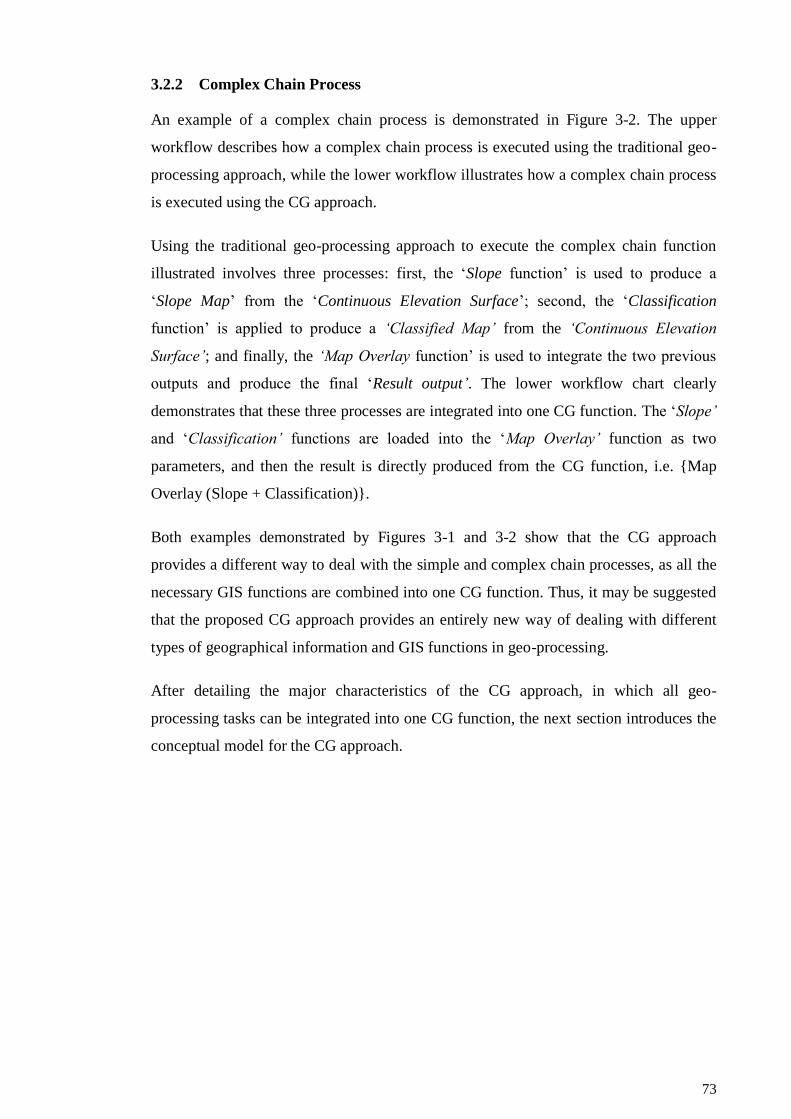
73
3.2.2 Complex Chain Process
An example of a complex chain process is demonstrated in Figure 3-2. The upper
workflow describes how a complex chain process is executed using the traditional geo-
processing approach, while the lower workflow illustrates how a complex chain process
is executed using the CG approach.
Using the traditional geo-processing approach to execute the complex chain function
illustrated involves three processes: first, the ‘Slope function’ is used to produce a
‘Slope Map’ from the ‘Continuous Elevation Surface’; second, the ‘Classification
function’ is applied to produce a ‘Classified Map’ from the ‘Continuous Elevation
Surface’; and finally, the ‘Map Overlay function’ is used to integrate the two previous
outputs and produce the final ‘Result output’. The lower workflow chart clearly
demonstrates that these three processes are integrated into one CG function. The ‘Slope’
and ‘Classification’ functions are loaded into the ‘Map Overlay’ function as two
parameters, and then the result is directly produced from the CG function, i.e. {Map
Overlay (Slope + Classification)}.
Both examples demonstrated by Figures 3-1 and 3-2 show that the CG approach
provides a different way to deal with the simple and complex chain processes, as all the
necessary GIS functions are combined into one CG function. Thus, it may be suggested
that the proposed CG approach provides an entirely new way of dealing with different
types of geographical information and GIS functions in geo-processing.
After detailing the major characteristics of the CG approach, in which all geo-
processing tasks can be integrated into one CG function, the next section introduces the
conceptual model for the CG approach.
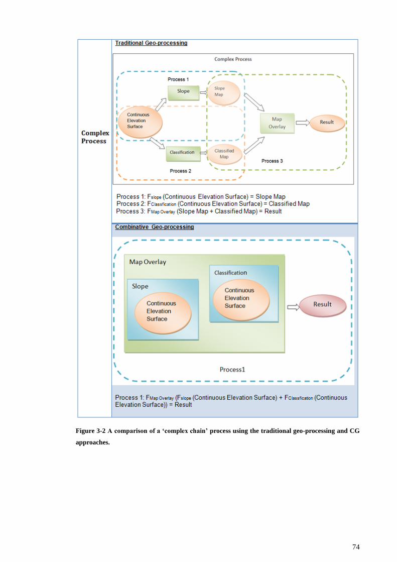
74
Figure 3-2 A comparison of a ‘complex chain’ process using the traditional geo-processing and CG
approaches.
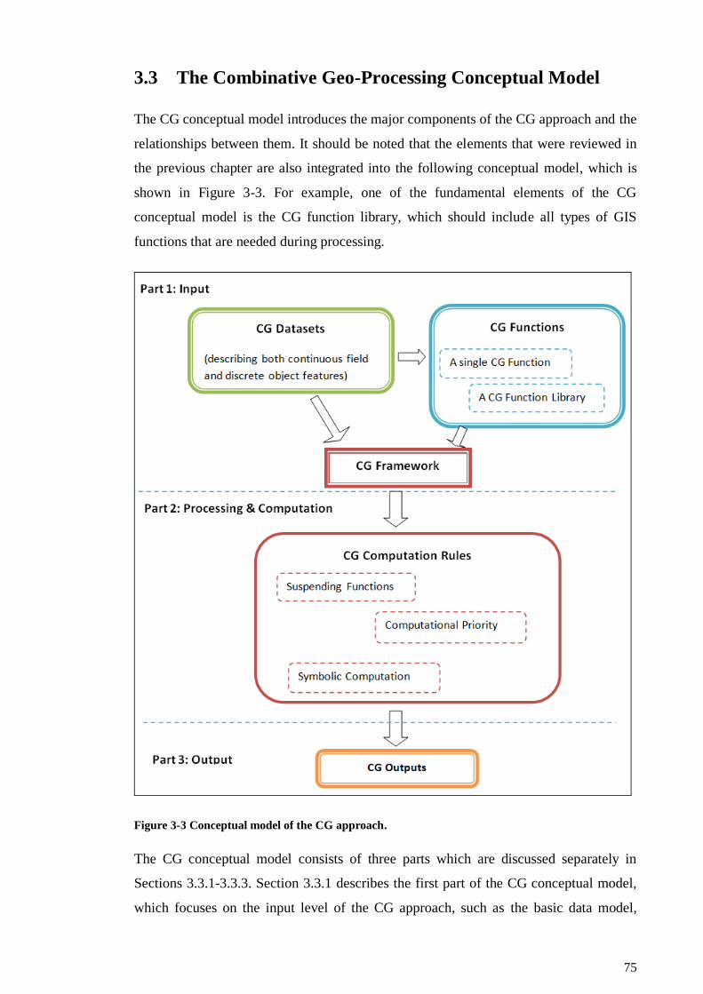
75
3.3 The Combinative Geo-Processing Conceptual Model
The CG conceptual model introduces the major components of the CG approach and the
relationships between them. It should be noted that the elements that were reviewed in
the previous chapter are also integrated into the following conceptual model, which is
shown in Figure 3-3. For example, one of the fundamental elements of the CG
conceptual model is the CG function library, which should include all types of GIS
functions that are needed during processing.
Figure 3-3 Conceptual model of the CG approach.
The CG conceptual model consists of three parts which are discussed separately in
Sections 3.3.1-3.3.3. Section 3.3.1 describes the first part of the CG conceptual model,
which focuses on the input level of the CG approach, such as the basic data model,

76
functions, and computation framework. Section 3.3.2 discusses the second part of the
CG conceptual model, which focuses on the processing and computation rules
employed in the CG approach. Finally, Section 3.3.3 describes the major characteristics
of the output or results of the proposed CG approach.
3.3.1 Input Level
There are three basic elements that a GIS user needs to consider before designing a geo-
processing model using the CG approach. The first element refers to the primary spatial
data model, as this influences many fundamental elements related to geo-processing,
e.g. data quality and computational efficiency. The second element refers to the CG
functions, as these are key components for building complex geo-processing models
using the CG approach. Finally, the third element is the CG framework, which
illustrates how to process CG datasets and CG functions using the proposed approach.
1) Combinative Geo-processing Dataset
An important concern of the proposed CG approach is the storage and representation of
spatial objects. In the previous chapter two main data types were discussed (i.e. vector
and raster data), and it was explained that vector data provides a popular way to
represent discrete objects, such as city boundaries and road networks, while raster data
can be used to show continuous fields, such as elevation models and land surface. At the
same time, it was also noted that both vector data and raster data representations have
limitations, such as for vector data a massive data storage space is required and the
algorithms for processing spatial analysis functions are complex, while for raster data a
very fine raster grid will represent sufficient detail but will require a large amount of
disk space.
As discussed in Section 2.3.4.1, the CG approach uses the point-based model concept to
represent spatial entities. In other words, the CG approach uses point data to represent
geographical features that include both discrete objects and continuous field features.
Point data plays an important role in GIS representations, as the majority of spatial data
are based on, or consist of, points.
The primary spatial data model in the CG approach involves points and the
mathematical model shown in Formula 3.1 is used to define a CG Dataset.
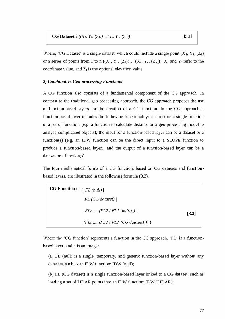
77
CG Dataset ϵ ((X1, Y1, (Z1))…(Xn, Yn, (Zn))) [3.1]
Where, ‘CG Dataset’ is a single dataset, which could include a single point (X1, Y1, (Z1)
or a series of points from 1 to n ((X1, Y1, (Z1))… (Xn, Yn, (Zn))). X1 and Y1 refer to the
coordinate value, and Z1 is the optional elevation value.
2) Combinative Geo-processing Functions
A CG function also consists of a fundamental component of the CG approach. In
contrast to the traditional geo-processing approach, the CG approach proposes the use
of function-based layers for the creation of a CG function. In the CG approach a
function-based layer includes the following functionality: it can store a single function
or a set of functions (e.g. a function to calculate distance or a geo-processing model to
analyse complicated objects); the input for a function-based layer can be a dataset or a
function(s) (e.g. an IDW function can be the direct input to a SLOPE function to
produce a function-based layer); and the output of a function-based layer can be a
dataset or a function(s).
The four mathematical forms of a CG function, based on CG datasets and function-
based layers, are illustrated in the following formula (3.2).
CG Function ϵ
[3.2]
Where the ‘CG function’ represents a function in the CG approach, ‘FL’ is a function-
based layer, and n is an integer.
(a) FL (null) is a single, temporary, and generic function-based layer without any
datasets, such as an IDW function: IDW (null);
(b) FL (CG dataset) is a single function-based layer linked to a CG dataset, such as
loading a set of LiDAR points into an IDW function: IDW (LiDAR);
{ FL (null) |
FL (CG dataset) |
(FLn…..(FL2 ( FL1 (null)))) |
(FLn…..(FL2 ( FL1 (CG dataset)))) }
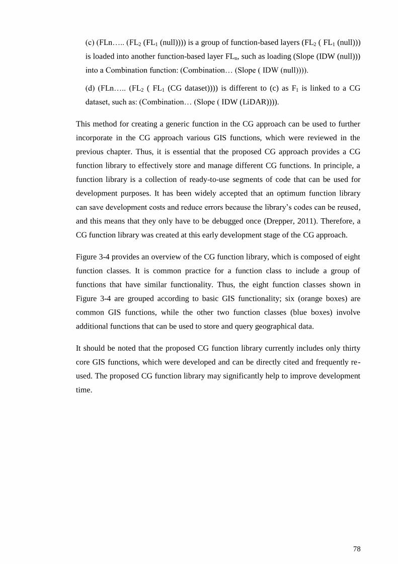
78
(c) (FLn….. (FL2 (FL1 (null)))) is a group of function-based layers (FL2 ( FL1 (null)))
is loaded into another function-based layer FLn, such as loading (Slope (IDW (null)))
into a Combination function: (Combination… (Slope ( IDW (null)))).
(d) (FLn….. (FL2 ( FL1 (CG dataset)))) is different to (c) as F1 is linked to a CG
dataset, such as: (Combination… (Slope ( IDW (LiDAR)))).
This method for creating a generic function in the CG approach can be used to further
incorporate in the CG approach various GIS functions, which were reviewed in the
previous chapter. Thus, it is essential that the proposed CG approach provides a CG
function library to effectively store and manage different CG functions. In principle, a
function library is a collection of ready-to-use segments of code that can be used for
development purposes. It has been widely accepted that an optimum function library
can save development costs and reduce errors because the library’s codes can be reused,
and this means that they only have to be debugged once (Drepper, 2011). Therefore, a
CG function library was created at this early development stage of the CG approach.
Figure 3-4 provides an overview of the CG function library, which is composed of eight
function classes. It is common practice for a function class to include a group of
functions that have similar functionality. Thus, the eight function classes shown in
Figure 3-4 are grouped according to basic GIS functionality; six (orange boxes) are
common GIS functions, while the other two function classes (blue boxes) involve
additional functions that can be used to store and query geographical data.
It should be noted that the proposed CG function library currently includes only thirty
core GIS functions, which were developed and can be directly cited and frequently re-
used. The proposed CG function library may significantly help to improve development
time.
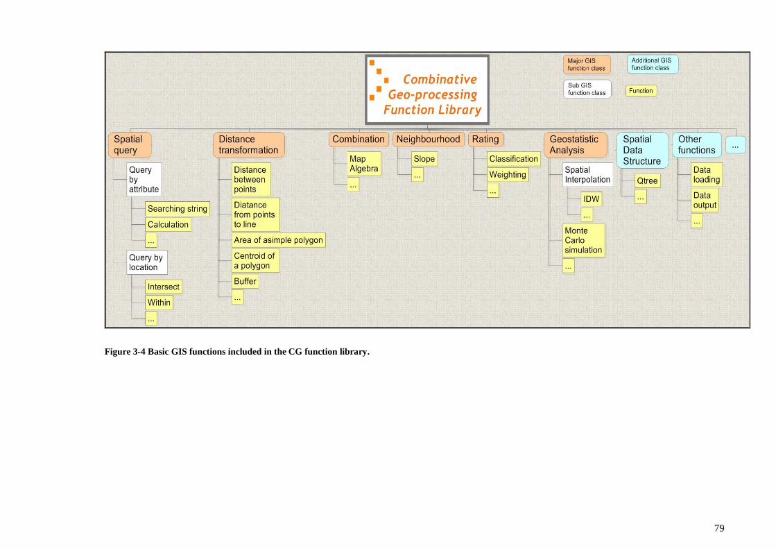
79
Figure 3-4 Basic GIS functions included in the CG function library.
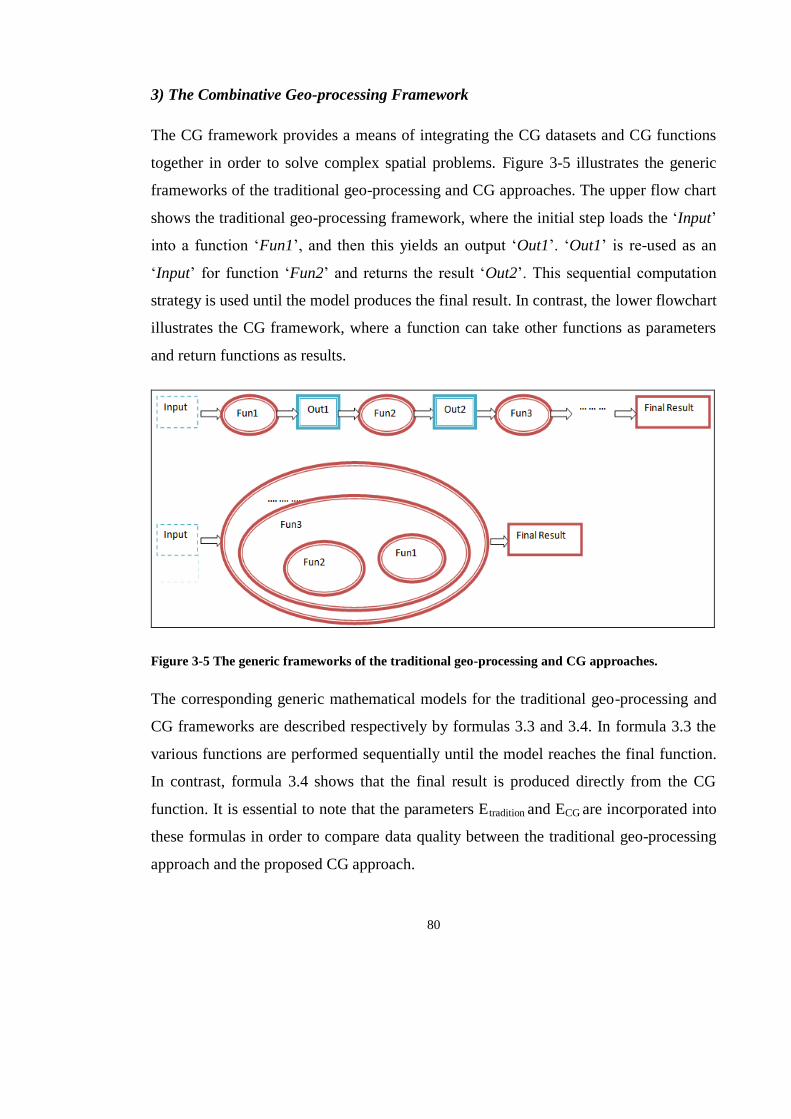
80
3) The Combinative Geo-processing Framework
The CG framework provides a means of integrating the CG datasets and CG functions
together in order to solve complex spatial problems. Figure 3-5 illustrates the generic
frameworks of the traditional geo-processing and CG approaches. The upper flow chart
shows the traditional geo-processing framework, where the initial step loads the ‘Input’
into a function ‘Fun1’, and then this yields an output ‘Out1’. ‘Out1’ is re-used as an
‘Input’ for function ‘Fun2’ and returns the result ‘Out2’. This sequential computation
strategy is used until the model produces the final result. In contrast, the lower flowchart
illustrates the CG framework, where a function can take other functions as parameters
and return functions as results.
Figure 3-5 The generic frameworks of the traditional geo-processing and CG approaches.
The corresponding generic mathematical models for the traditional geo-processing and
CG frameworks are described respectively by formulas 3.3 and 3.4. In formula 3.3 the
various functions are performed sequentially until the model reaches the final function.
In contrast, formula 3.4 shows that the final result is produced directly from the CG
function. It is essential to note that the parameters Etradition and ECG are incorporated into
these formulas in order to compare data quality between the traditional geo-processing
approach and the proposed CG approach.

81
[3.3]
In formula 3.3, the ‘dataset’ is the input, which can be raster or vector data, and ‘F1, F2,
F3, …, Fi’ represent different types of GIS functions, such as data interpolation, map
algebra, vectorisation and network analysis. ‘O1, O2, O3, …, Oi’ are the various outputs
based on the numerical computations and approximated value, while ‘E1, E2, E3, …, Ei’
represent the potential errors accompanying each single stage of the sequential
computation. ‘Etradition’ represents the potential errors in the traditional geo-processing
approach. Finally, represents the computation progress, represents the
‘stage by stage’ computation strategy, and describes the last step in the entire
framework.
[3.4]
In formula 3.4, ‘CG dataset’ is the input, and ‘FL1, FL2, FL3, …, FLi’ represent the
different types of function-based layers in the CG approach. The ‘CG function’

82
represents a combinative function which includes all function-based layers (i.e. FL1,
FL2, FL3, …, FLi). ‘ECG’ represents the potential error in the CG approach. Moreover, a
recursive algorithm will be applied in this formula to execute the functions from FL1 to
FLi.
It should be noted that this thesis attempts to compare the difference between ‘E tradition’
and ‘ECG’, something which is discussed further in Chapters 5 and 6, where different
case studies are presented with the aim of investigating the data quality of the CG
implementations.
3.3.2 Processing and Computation
Following the discussion on the fundamental components of the CG approach, this
section discusses the processing and computational issues, and explains how the CG
framework can be evaluated in the proposed approach.
An ideal CG framework needs a reliable way to operate and evaluate various CG
datasets and CG functions, thus a set of CG computational rules is introduced, which
include ‘suspending’, ‘computation priority’, and ‘symbolic computation’. Notably,
these computation rules essentially constitute the key difference between the CG
approach and the traditional geo-processing approach.
‘Suspending’ is a method which can help manage a CG function. All CG functions in a
geo-processing model can be suspended until a GIS needs them for producing the
results. Suspending can further help to understand a basic difference between the
traditional geo-processing and CG approaches. As illustrated in Figures 3-1 and 3-2, the
traditional geo-processing approach uses a sequential computation strategy, with each
function returning a specific result; therefore the final result will only be calculated
when all the functions have been executed. In contrast, using the CG approach the input
datasets are temporarily stored in the function-based layers and calculations are
suspended until the user defines the parameters of the final result or requests the value
83
of a function at a specific location. Thus, computations will only commence when
requested by the end user, and this is when the final result will be calculated.
It should be noted that there are two main advantages to suspended functions. First, the
CG-enabled GIS does not need to use extra memory space to store intermediary results
during the computation processes. Second, functions are only executed when users
require the final results, which may reduce the total computational period and introduce
fewer errors, especially when compared with the errors that can be generated when there
are several intermediary steps involved (Haklay, 2004). These aspects are explored in
later in this thesis.
The second rule refers to ‘computation priority’, and it is similar to the priority rule used
in mathematics. When functions are suspended in a geo-processing model the CG
approach needs to decide which spatial function will be executed first. The aim is to
provide an optimum computational sequence for implementing a set of spatial functions
at a lower computational cost. A typical example of a priority-based computation is that
of algorithm scheduling, which is concerned with the optimal allocation of scarce
resources to activities over time. When there are many spatial functions that need to be
executed (e.g. in Figure 3-2 the functions ‘Slope’, ‘Classification’ and ‘Map Overlay’
all needed to be executed), the computational priority should make a judgment
concerning which function should be performed first. Computational priority helps to
further define in what order the functions will be executed until the entire set of
functions is finally executed as efficiently as possible.
The third rule refers to symbolic computation. In contrast to the traditional geo-
processing approach, where functions are evaluated using numerical calculations and
approximate values, the CG approach uses symbolic computation to calculate the CG
functions. As discussed in Section 2.3.4.2, symbolic computation provides an exact
method for mathematical calculation.
84
3.3.3 Outputs and Results
The last part of the proposed CG conceptual model is concerned with the production of
the final result. There are two alternative formats in the CG approach for producing a
final output and which further differentiate it from the traditional geo-processing
approach.
The first format of the final result is points, which is due to the fact that the primary
spatial data model of the CG approach involves the use of points. GIS users can process
these points straightforwardly or transform them into other spatial data models, such as
raster and vector data, for further computations.
The second format of the final result is functions, because the way CG functions are
operated by higher-order functions could produce new functions from existing
functions. In other words a CG function can produce a function or a set of functions as
the final outcome. Consequently, the functions can be reused or can be used as the input
for other geo-processing models for advanced spatial analysis.
Formula 3.5 defines the CG output in two different forms.
CG Output ϵ ( {(X1, Y1, (A1, …, Am))…(Xn, Yn, (An, …, Am))} |
{CG functions} ) [3.5]
Where ‘(X1, Y1, (A1, …, Am)’ represents an output point location (X1, Y1) with a single or
several attributes ‘(A1, …, Am)’. n and m are both integers.
The major components of the conceptual model of the CG approach have now been
described and the next section discusses the strengths and also potential limitations of
the CG approach.
85
3.4 Potential Advantages and Disadvantages of the
Combinative Geo-Processing Approach
The previous sections have explained some of the advantages of the proposed CG
approach over the traditional geo-processing approach, which include the final output
being directly produced from a CG function. One of the benefits of this is that the CG-
enabled GIS does not need to produce any intermediary results. In addition, in CG-
enabled GIS there is no need to convert geographical data in different spatial data
models, such raster and vector data, because all the CG datasets are stored as points and
all the computations and manipulations use points. For example, in the traditional geo-
processing approach two conversion steps are needed to convert LiDAR to a DEM
image, and convert a DEM image to a contour map in order to implement this task,
while the CG approach can produce a contour map using LiDAR points directly.
The CG approach provides more flexibility in terms of producing a final result. For
example, in existing GIS tools the resolution and extent (or study area) of the final
results are the default values and are defined by the system when users run a layer
combination operation. However, the CG approach can provide a flexibility in the final
result creation. For instance, the resolution can be defined by the user and the extent can
be based on a five metre buffer of residential area.
Finally, when users calculate different CG functions in a CG-enabled GIS, all the
computations run on computer random access memory (RAM) are faster, while the
traditional approach may take longer. This is because the traditional geo-processing
approach needs to access, query, and save multi-step results on locally available storage.
Although the proposed CG approach has the potential to significantly improve the
performance of geo-processing, there are still two significant concerns that should be
noted and the remainder of this thesis aims to address these specific concerns.
The first concern refers to the development period. The fact that geo-processing is an
integrated platform means that the tasks include not only the GIS functions, but also
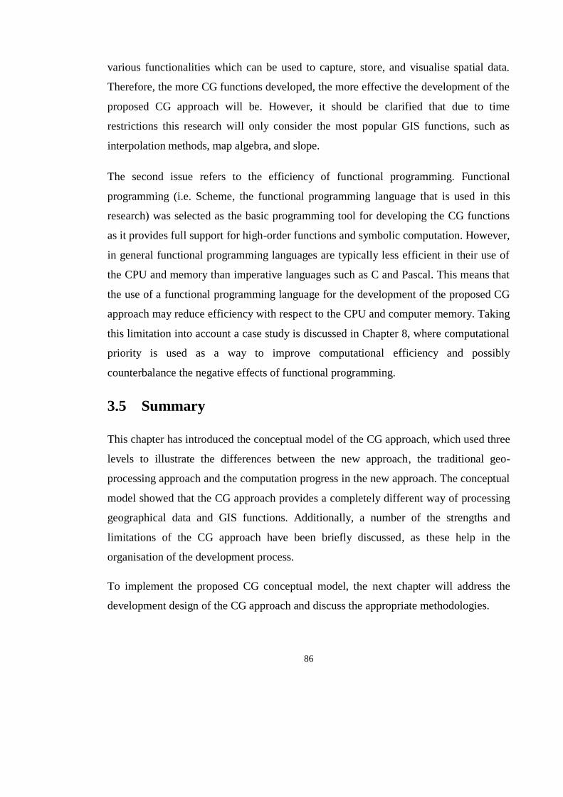
86
various functionalities which can be used to capture, store, and visualise spatial data.
Therefore, the more CG functions developed, the more effective the development of the
proposed CG approach will be. However, it should be clarified that due to time
restrictions this research will only consider the most popular GIS functions, such as
interpolation methods, map algebra, and slope.
The second issue refers to the efficiency of functional programming. Functional
programming (i.e. Scheme, the functional programming language that is used in this
research) was selected as the basic programming tool for developing the CG functions
as it provides full support for high-order functions and symbolic computation. However,
in general functional programming languages are typically less efficient in their use of
the CPU and memory than imperative languages such as C and Pascal. This means that
the use of a functional programming language for the development of the proposed CG
approach may reduce efficiency with respect to the CPU and computer memory. Taking
this limitation into account a case study is discussed in Chapter 8, where computational
priority is used as a way to improve computational efficiency and possibly
counterbalance the negative effects of functional programming.
3.5 Summary
This chapter has introduced the conceptual model of the CG approach, which used three
levels to illustrate the differences between the new approach, the traditional geo-
processing approach and the computation progress in the new approach. The conceptual
model showed that the CG approach provides a completely different way of processing
geographical data and GIS functions. Additionally, a number of the strengths and
limitations of the CG approach have been briefly discussed, as these help in the
organisation of the development process.
To implement the proposed CG conceptual model, the next chapter will address the
development design of the CG approach and discuss the appropriate methodologies.
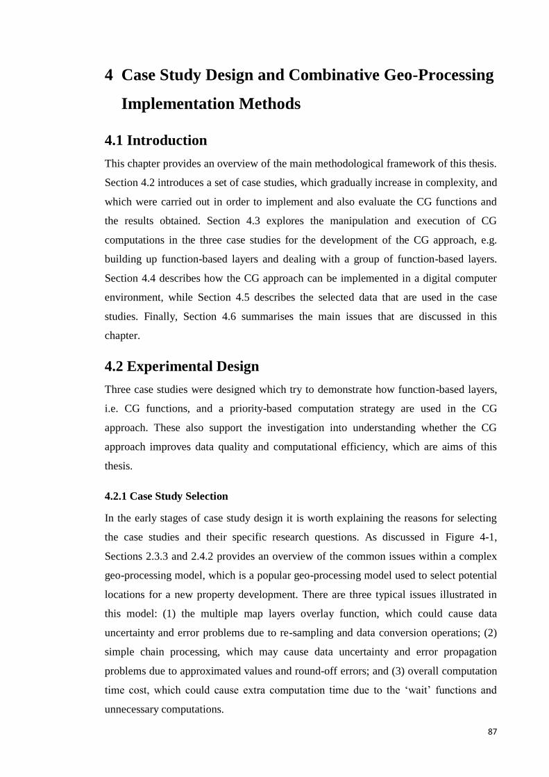
87
4 Case Study Design and Combinative Geo-Processing
Implementation Methods
4.1 Introduction
This chapter provides an overview of the main methodological framework of this thesis.
Section 4.2 introduces a set of case studies, which gradually increase in complexity, and
which were carried out in order to implement and also evaluate the CG functions and
the results obtained. Section 4.3 explores the manipulation and execution of CG
computations in the three case studies for the development of the CG approach, e.g.
building up function-based layers and dealing with a group of function-based layers.
Section 4.4 describes how the CG approach can be implemented in a digital computer
environment, while Section 4.5 describes the selected data that are used in the case
studies. Finally, Section 4.6 summarises the main issues that are discussed in this
chapter.
4.2 Experimental Design
Three case studies were designed which try to demonstrate how function-based layers,
i.e. CG functions, and a priority-based computation strategy are used in the CG
approach. These also support the investigation into understanding whether the CG
approach improves data quality and computational efficiency, which are aims of this
thesis.
4.2.1 Case Study Selection
In the early stages of case study design it is worth explaining the reasons for selecting
the case studies and their specific research questions. As discussed in Figure 4-1,
Sections 2.3.3 and 2.4.2 provides an overview of the common issues within a complex
geo-processing model, which is a popular geo-processing model used to select potential
locations for a new property development. There are three typical issues illustrated in
this model: (1) the multiple map layers overlay function, which could cause data
uncertainty and error problems due to re-sampling and data conversion operations; (2)
simple chain processing, which may cause data uncertainty and error propagation
problems due to approximated values and round-off errors; and (3) overall computation
time cost, which could cause extra computation time due to the ‘wait’ functions and
unnecessary computations.
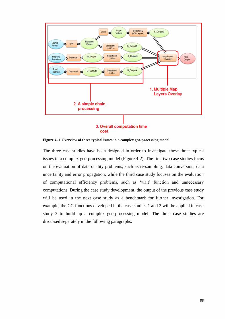
88
Figure 4- 1 Overview of three typical issues in a complex geo-processing model.
The three case studies have been designed in order to investigate these three typical
issues in a complex geo-processing model (Figure 4-2). The first two case studies focus
on the evaluation of data quality problems, such as re-sampling, data conversion, data
uncertainty and error propagation, while the third case study focuses on the evaluation
of computational efficiency problems, such as ‘wait’ function and unnecessary
computations. During the case study development, the output of the previous case study
will be used in the next case study as a benchmark for further investigation. For
example, the CG functions developed in the case studies 1 and 2 will be applied in case
study 3 to build up a complex geo-processing model. The three case studies are
discussed separately in the following paragraphs.
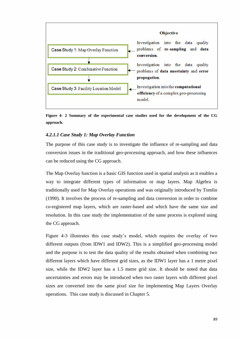
89
Figure 4- 2 Summary of the experimental case studies used for the development of the CG
approach.
4.2.1.1 Case Study 1: Map Overlay Function
The purpose of this case study is to investigate the influence of re-sampling and data
conversion issues in the traditional geo-processing approach, and how these influences
can be reduced using the CG approach.
The Map Overlay function is a basic GIS function used in spatial analysis as it enables a
way to integrate different types of information or map layers. Map Algebra is
traditionally used for Map Overlay operations and was originally introduced by Tomlin
(1990). It involves the process of re-sampling and data conversion in order to combine
co-registered map layers, which are raster-based and which have the same size and
resolution. In this case study the implementation of the same process is explored using
the CG approach.
Figure 4-3 illustrates this case study’s model, which requires the overlay of two
different outputs (from IDW1 and IDW2). This is a simplified geo-processing model
and the purpose is to test the data quality of the results obtained when combining two
different layers which have different grid sizes, as the IDW1 layer has a 1 metre pixel
size, while the IDW2 layer has a 1.5 metre grid size. It should be noted that data
uncertainties and errors may be introduced when two raster layers with different pixel
sizes are converted into the same pixel size for implementing Map Layers Overlay
operations. This case study is discussed in Chapter 5.
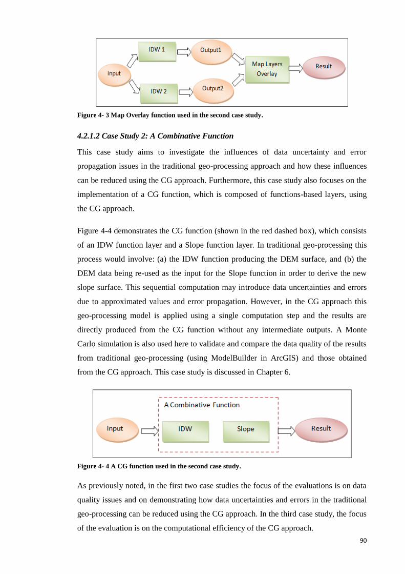
90
Figure 4- 3 Map Overlay function used in the second case study.
4.2.1.2 Case Study 2: A Combinative Function
This case study aims to investigate the influences of data uncertainty and error
propagation issues in the traditional geo-processing approach and how these influences
can be reduced using the CG approach. Furthermore, this case study also focuses on the
implementation of a CG function, which is composed of functions-based layers, using
the CG approach.
Figure 4-4 demonstrates the CG function (shown in the red dashed box), which consists
of an IDW function layer and a Slope function layer. In traditional geo-processing this
process would involve: (a) the IDW function producing the DEM surface, and (b) the
DEM data being re-used as the input for the Slope function in order to derive the new
slope surface. This sequential computation may introduce data uncertainties and errors
due to approximated values and error propagation. However, in the CG approach this
geo-processing model is applied using a single computation step and the results are
directly produced from the CG function without any intermediate outputs. A Monte
Carlo simulation is also used here to validate and compare the data quality of the results
from traditional geo-processing (using ModelBuilder in ArcGIS) and those obtained
from the CG approach. This case study is discussed in Chapter 6.
Figure 4- 4 A CG function used in the second case study.
As previously noted, in the first two case studies the focus of the evaluations is on data
quality issues and on demonstrating how data uncertainties and errors in the traditional
geo-processing can be reduced using the CG approach. In the third case study, the focus
of the evaluation is on the computational efficiency of the CG approach.
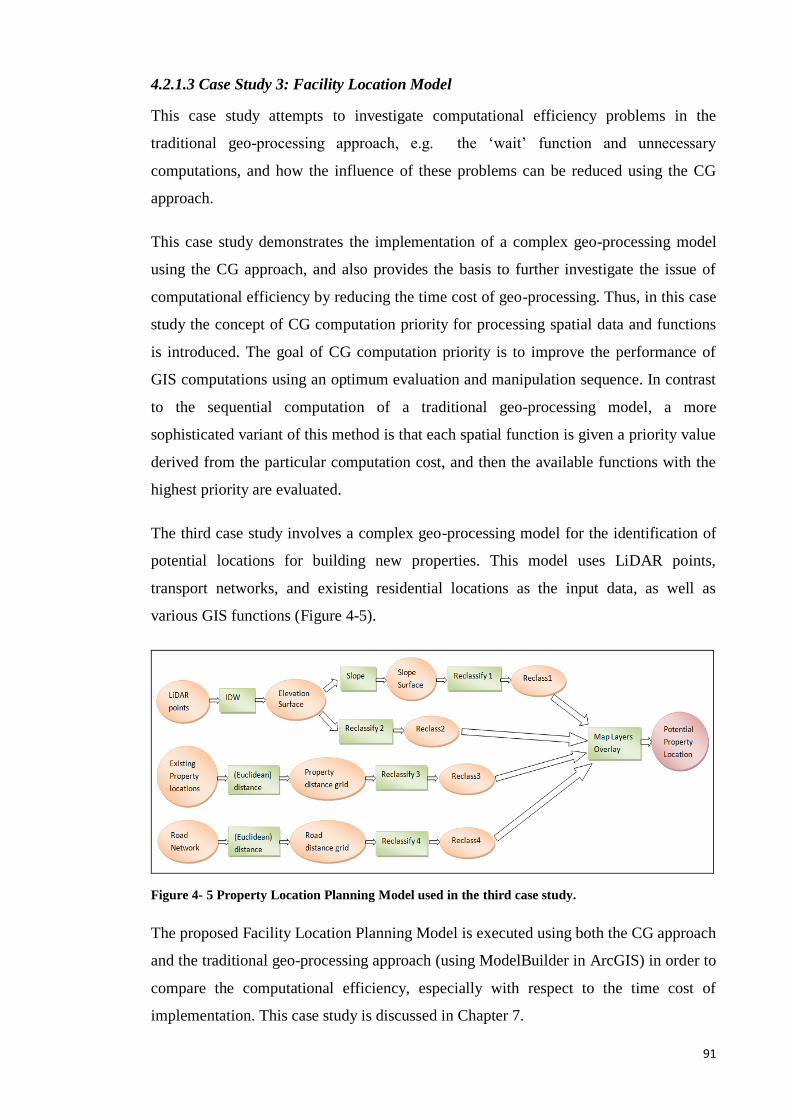
91
4.2.1.3 Case Study 3: Facility Location Model
This case study attempts to investigate computational efficiency problems in the
traditional geo-processing approach, e.g. the ‘wait’ function and unnecessary
computations, and how the influence of these problems can be reduced using the CG
approach.
This case study demonstrates the implementation of a complex geo-processing model
using the CG approach, and also provides the basis to further investigate the issue of
computational efficiency by reducing the time cost of geo-processing. Thus, in this case
study the concept of CG computation priority for processing spatial data and functions
is introduced. The goal of CG computation priority is to improve the performance of
GIS computations using an optimum evaluation and manipulation sequence. In contrast
to the sequential computation of a traditional geo-processing model, a more
sophisticated variant of this method is that each spatial function is given a priority value
derived from the particular computation cost, and then the available functions with the
highest priority are evaluated.
The third case study involves a complex geo-processing model for the identification of
potential locations for building new properties. This model uses LiDAR points,
transport networks, and existing residential locations as the input data, as well as
various GIS functions (Figure 4-5).
Figure 4- 5 Property Location Planning Model used in the third case study.
The proposed Facility Location Planning Model is executed using both the CG approach
and the traditional geo-processing approach (using ModelBuilder in ArcGIS) in order to
compare the computational efficiency, especially with respect to the time cost of
implementation. This case study is discussed in Chapter 7.
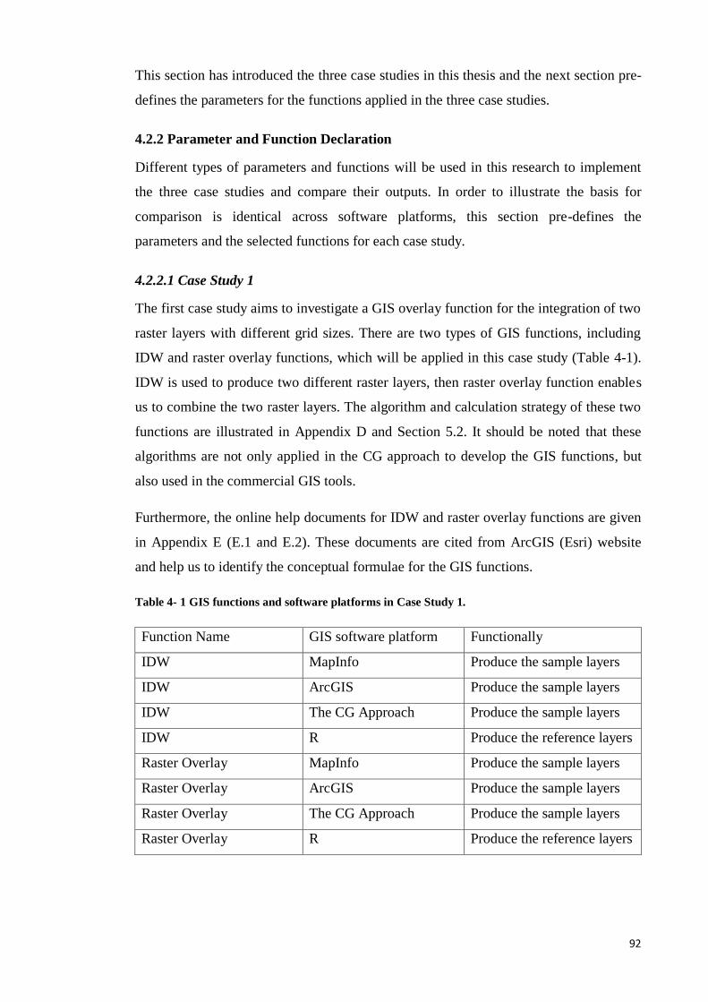
92
This section has introduced the three case studies in this thesis and the next section pre-
defines the parameters for the functions applied in the three case studies.
4.2.2 Parameter and Function Declaration
Different types of parameters and functions will be used in this research to implement
the three case studies and compare their outputs. In order to illustrate the basis for
comparison is identical across software platforms, this section pre-defines the
parameters and the selected functions for each case study.
4.2.2.1 Case Study 1
The first case study aims to investigate a GIS overlay function for the integration of two
raster layers with different grid sizes. There are two types of GIS functions, including
IDW and raster overlay functions, which will be applied in this case study (Table 4-1).
IDW is used to produce two different raster layers, then raster overlay function enables
us to combine the two raster layers. The algorithm and calculation strategy of these two
functions are illustrated in Appendix D and Section 5.2. It should be noted that these
algorithms are not only applied in the CG approach to develop the GIS functions, but
also used in the commercial GIS tools.
Furthermore, the online help documents for IDW and raster overlay functions are given
in Appendix E (E.1 and E.2). These documents are cited from ArcGIS (Esri) website
and help us to identify the conceptual formulae for the GIS functions.
Table 4- 1 GIS functions and software platforms in Case Study 1.
Function Name GIS software platform Functionally
IDW MapInfo Produce the sample layers
IDW ArcGIS Produce the sample layers
IDW The CG Approach Produce the sample layers
IDW R Produce the reference layers
Raster Overlay MapInfo Produce the sample layers
Raster Overlay ArcGIS Produce the sample layers
Raster Overlay The CG Approach Produce the sample layers
Raster Overlay R Produce the reference layers
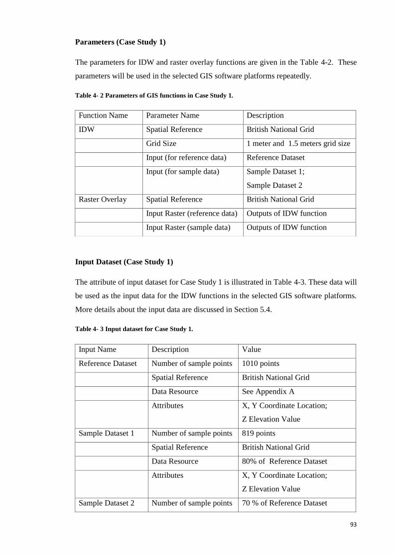
93
Parameters (Case Study 1)
The parameters for IDW and raster overlay functions are given in the Table 4-2. These
parameters will be used in the selected GIS software platforms repeatedly.
Table 4- 2 Parameters of GIS functions in Case Study 1.
Input Dataset (Case Study 1)
The attribute of input dataset for Case Study 1 is illustrated in Table 4-3. These data will
be used as the input data for the IDW functions in the selected GIS software platforms.
More details about the input data are discussed in Section 5.4.
Table 4- 3 Input dataset for Case Study 1.
Function Name Parameter Name Description
IDW Spatial Reference British National Grid
Grid Size 1 meter and 1.5 meters grid size
Input (for reference data) Reference Dataset
Input (for sample data) Sample Dataset 1;
Sample Dataset 2
Raster Overlay Spatial Reference British National Grid
Input Raster (reference data) Outputs of IDW function
Input Raster (sample data) Outputs of IDW function
Input Name Description Value
Reference Dataset Number of sample points 1010 points
Spatial Reference British National Grid
Data Resource See Appendix A
Attributes X, Y Coordinate Location;
Z Elevation Value
Sample Dataset 1 Number of sample points 819 points
Spatial Reference British National Grid
Data Resource 80% of Reference Dataset
Attributes X, Y Coordinate Location;
Z Elevation Value
Sample Dataset 2 Number of sample points 70 % of Reference Dataset
94
Comparison Method (Case Study 1)
The map algebra and statistical analysis are used in this case study to exam the outputs.
Produced from the GIS software platforms. Raster Algebra’s minus function subtracts
the value of the second input raster from the value of the first input raster on a cell-by-
cell basis and supports investigating the difference of grid cells between the actual,
observed values that are stored in the Integrated Reference Layers (IRLs) and the
derived values that are stored in Integrated Sample Layers (ISLs). Furthermore,
statistical analysis was also undertaken in order to compare the Raster Algebra (Minus)
results in more detail. For the purposes of this comparison, the Maximum (Max),
Minimum (Min), and the Standard Deviation values are used. The results of
comparison, such as the key discrepancies of outputs, are discussed in Section 5.7.
4.2.2.2 Case Study 2
The second case study focuses on a simple chain processing, which includes two GIS
functions: IDW and slope (Table 4-4). IDW is used to produce elevation value from
point data, and slope is applied to produce a surface model from the elevation value. In
addition to IDW, the algorithm and calculation strategy of slope function is discussed in
Section 6.2.1 and Appendix E (E.3). It should be noted that this algorithm is not only
applied in the commercial GIS software platforms (e.g. ArcGIS), also used in the CG
approach to develop the slope function.
Spatial Reference British National Grid
Data Resource See Appendix A
Attributes X, Y Coordinate Location;
Z Elevation Value
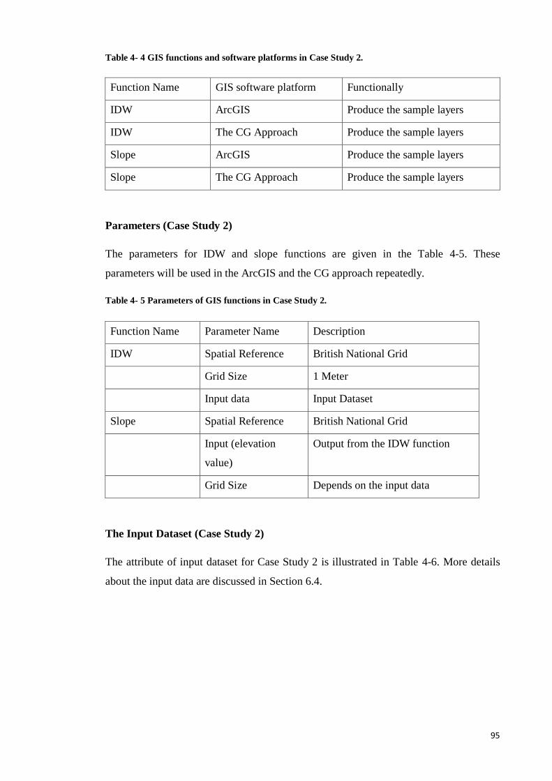
95
Table 4- 4 GIS functions and software platforms in Case Study 2.
Function Name GIS software platform Functionally
IDW ArcGIS Produce the sample layers
IDW The CG Approach Produce the sample layers
Slope ArcGIS Produce the sample layers
Slope The CG Approach Produce the sample layers
Parameters (Case Study 2)
The parameters for IDW and slope functions are given in the Table 4-5. These
parameters will be used in the ArcGIS and the CG approach repeatedly.
Table 4- 5 Parameters of GIS functions in Case Study 2.
The Input Dataset (Case Study 2)
The attribute of input dataset for Case Study 2 is illustrated in Table 4-6. More details
about the input data are discussed in Section 6.4.
Function Name Parameter Name Description
IDW Spatial Reference British National Grid
Grid Size 1 Meter
Input data Input Dataset
Slope Spatial Reference British National Grid
Input (elevation
value)
Output from the IDW function
Grid Size Depends on the input data

96
Table 4- 6 Input dataset for Case Study 2.
Input Name Description Value
Input Dataset Number of sample points 26499 points
Spatial Reference British National Grid
Data Resource See Appendix A
Attribute X, Y Coordinate Location;
Z Elevation Value
The Comparison Method (Case Study 2)
In this case study, Monte Carlo simulation is used to calculate the results’ mean and
variance in order to investigate the impact of data uncertainties on data quality in both
simple chain processing model implementations, including ArcGIS and the CG
approach. Table 4-7 illustrates the primary parameters of Monte Carlo simulation. The
details about the computation strategy and comparison results are discussed in Section
6.7.
Table 4- 7 Primary parameters for Monte Carlo simulation in Case Study 2.
Parameter Name Description
Input data Randomly select 60% of raw LiDAR points
(Input Dataset)
Output data Slope values
Iterations 50 times
4.2.2.3 Case Study 3
The third case study focuses on a complex chain processing, which includes five types
of GIS functions: IDW, slope, selection, distance, and map layer overlay (Raster) (Table
4-8). In addition to IDW, slope, and map layer overlay (Raster), the computation
algorithms of selection and distance are illustrated in the Appendix E (E.4 and E.5).
These algorithms are used in both GIS software platforms (ArcGIS and the CG
approach) in the third case study.
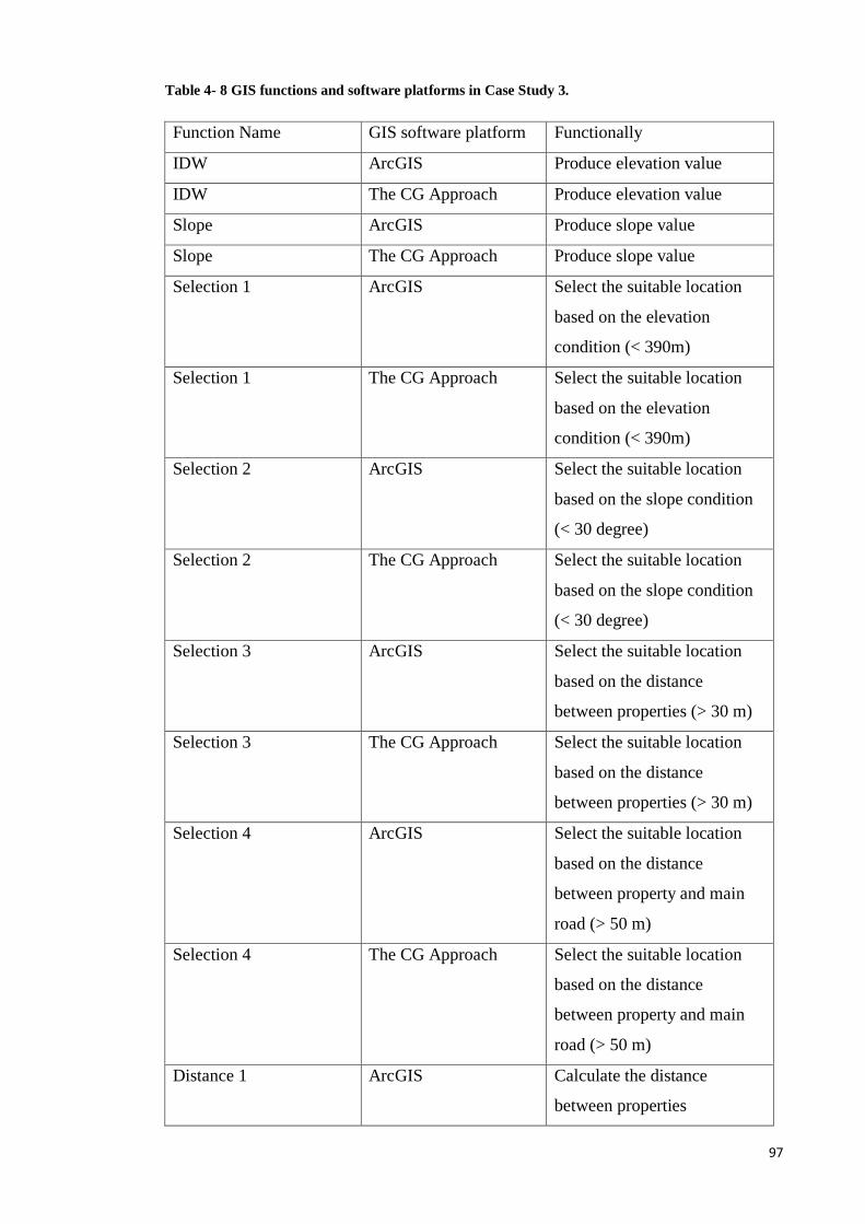
97
Table 4- 8 GIS functions and software platforms in Case Study 3.
Function Name GIS software platform Functionally
IDW ArcGIS Produce elevation value
IDW The CG Approach Produce elevation value
Slope ArcGIS Produce slope value
Slope The CG Approach Produce slope value
Selection 1 ArcGIS Select the suitable location
based on the elevation
condition (< 390m)
Selection 1 The CG Approach Select the suitable location
based on the elevation
condition (< 390m)
Selection 2 ArcGIS Select the suitable location
based on the slope condition
(< 30 degree)
Selection 2 The CG Approach Select the suitable location
based on the slope condition
(< 30 degree)
Selection 3 ArcGIS Select the suitable location
based on the distance
between properties (> 30 m)
Selection 3 The CG Approach Select the suitable location
based on the distance
between properties (> 30 m)
Selection 4 ArcGIS Select the suitable location
based on the distance
between property and main
road (> 50 m)
Selection 4 The CG Approach Select the suitable location
based on the distance
between property and main
road (> 50 m)
Distance 1 ArcGIS Calculate the distance
between properties
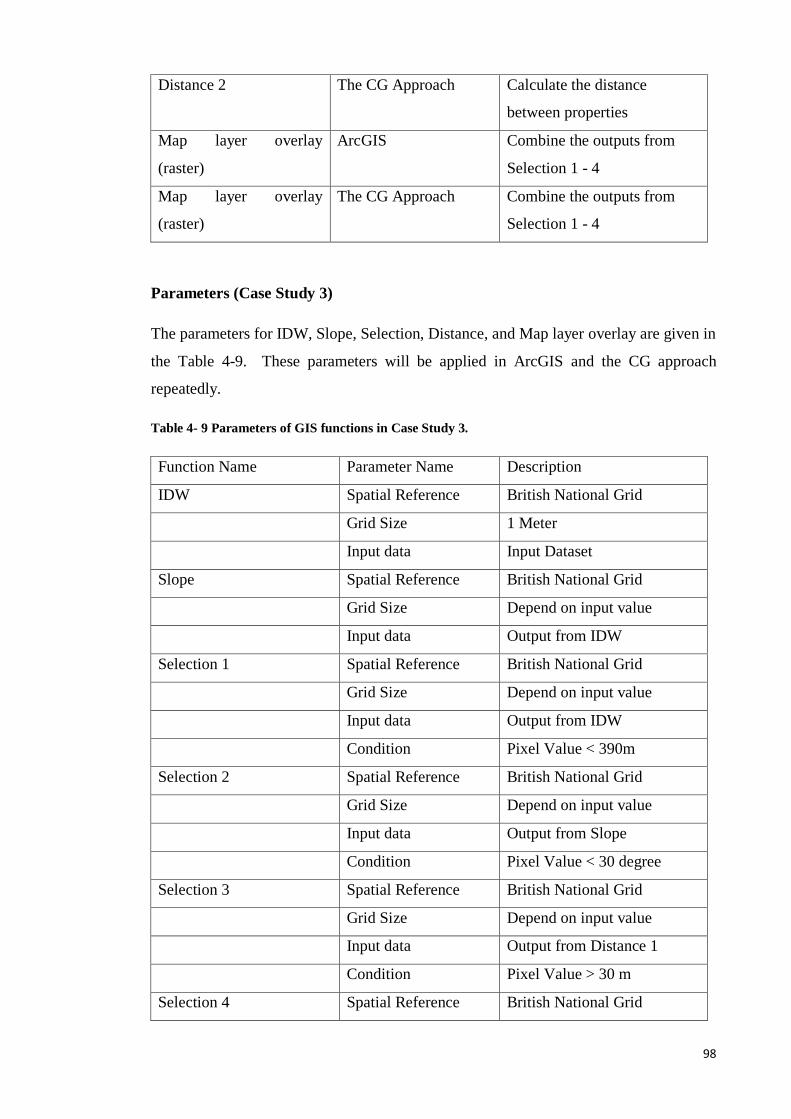
98
Distance 2 The CG Approach Calculate the distance
between properties
Map layer overlay
(raster)
ArcGIS Combine the outputs from
Selection 1 - 4
Map layer overlay
(raster)
The CG Approach Combine the outputs from
Selection 1 - 4
Parameters (Case Study 3)
The parameters for IDW, Slope, Selection, Distance, and Map layer overlay are given in
the Table 4-9. These parameters will be applied in ArcGIS and the CG approach
repeatedly.
Table 4- 9 Parameters of GIS functions in Case Study 3.
Function Name Parameter Name Description
IDW Spatial Reference British National Grid
Grid Size 1 Meter
Input data Input Dataset
Slope Spatial Reference British National Grid
Grid Size Depend on input value
Input data Output from IDW
Selection 1 Spatial Reference British National Grid
Grid Size Depend on input value
Input data Output from IDW
Condition Pixel Value < 390m
Selection 2 Spatial Reference British National Grid
Grid Size Depend on input value
Input data Output from Slope
Condition Pixel Value < 30 degree
Selection 3 Spatial Reference British National Grid
Grid Size Depend on input value
Input data Output from Distance 1
Condition Pixel Value > 30 m
Selection 4 Spatial Reference British National Grid
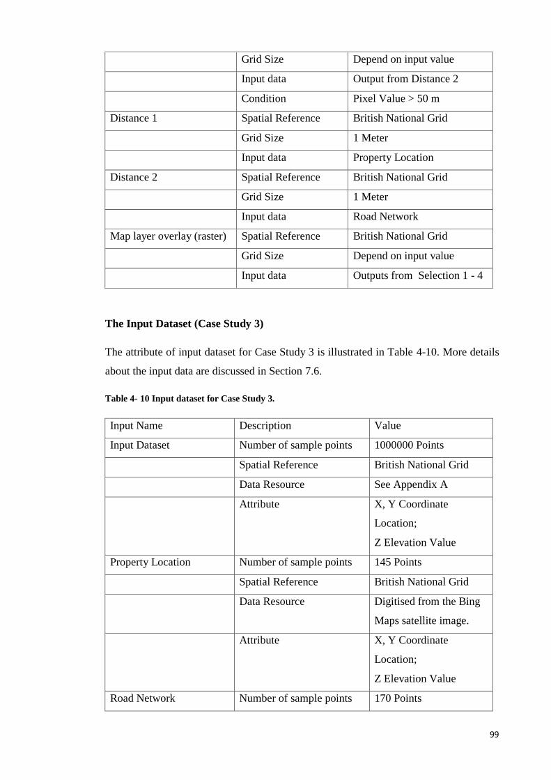
99
Grid Size Depend on input value
Input data Output from Distance 2
Condition Pixel Value > 50 m
Distance 1 Spatial Reference British National Grid
Grid Size 1 Meter
Input data Property Location
Distance 2 Spatial Reference British National Grid
Grid Size 1 Meter
Input data Road Network
Map layer overlay (raster) Spatial Reference British National Grid
Grid Size Depend on input value
Input data Outputs from Selection 1 - 4
The Input Dataset (Case Study 3)
The attribute of input dataset for Case Study 3 is illustrated in Table 4-10. More details
about the input data are discussed in Section 7.6.
Table 4- 10 Input dataset for Case Study 3.
Input Name Description Value
Input Dataset Number of sample points 1000000 Points
Spatial Reference British National Grid
Data Resource See Appendix A
Attribute X, Y Coordinate
Location;
Z Elevation Value
Property Location Number of sample points 145 Points
Spatial Reference British National Grid
Data Resource Digitised from the Bing
Maps satellite image.
Attribute X, Y Coordinate
Location;
Z Elevation Value
Road Network Number of sample points 170 Points
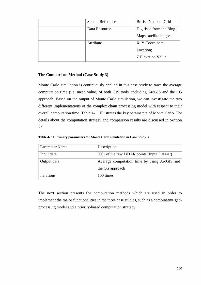
100
Spatial Reference British National Grid
Data Resource Digitised from the Bing
Maps satellite image.
Attribute X, Y Coordinate
Location;
Z Elevation Value
The Comparison Method (Case Study 3)
Monte Carlo simulation is continuously applied in this case study to trace the average
computation time (i.e. mean value) of both GIS tools, including ArcGIS and the CG
approach. Based on the output of Monte Carlo simulation, we can investigate the two
different implementations of the complex chain processing model with respect to their
overall computation time. Table 4-11 illustrates the key parameters of Monte Carlo. The
details about the computation strategy and comparison results are discussed in Section
7.9.
Table 4- 11 Primary parameters for Monte Carlo simulation in Case Study 3.
Parameter Name Description
Input data 90% of the raw LiDAR points (Input Dataset)
Output data Average computation time by using ArcGIS and
the CG approach
Iterations 100 times
The next section presents the computation methods which are used in order to
implement the major functionalities in the three case studies, such as a combinative geo-
processing model and a priority-based computation strategy.

101
4.3 Methods Used in Combinative Geo-processing Function
Execution
The three case studies implementation requests a set of methods in the CG approach to
manipulate and execute the CG functions. The basic methods applied in the CG
approach were introduced in Chapter 3, such as symbolic computation. Therefore, this
section focuses on the computation methods applied in the CG approach practically,
with respect to the development of the ‘CG function’ and a ‘priority-based computation
strategy’. The CG function enables a basic way to implement the function-based layer
together with an attempt to improve data quality, while the priority-based computation
strategy is a key method for computational efficiency improvement.
It was also noted in Sections 3.2 and 3.3 that there are two main characteristics of the
proposed CG approach that differentiate it from traditional geo-processing: first, a CG
function is used to implement the entire geo-processing model; and second, a priority
sequence is used for the execution of the CG functions. To achieve these two
characteristics the CG approach uses the concepts and functionality of ‘Higher-Order
Function’, ‘Recursive Algorithms’ and ‘Lazy Evaluation’, which are discussed in the
following sections.
4.3.1 Higher-Order Function
A Higher-Order Function is a function which takes functions as parameters and returns
functions as results (Dybvig, 2002). A pseudo-code to demonstrate how Higher-Order
Functions are executed is provided below:
Step1: define the first Higher-Order ‘Function1’ Function1(x)= x +9;
Step2: define the second Higher-Order ‘Function2’ Function2 (fun, x) = fun (x) * fun
(x)
Where the input is ‘fun’ (i.e. function) and a value ‘x’ and output is ‘fun (x) * fun (x)’
After defining Higher-Order Functions, i.e. Function1 and Function2, users can run a
calculation similar to the example below:
Function2 (Function1, 7) → ((7 + 9)*(7 + 9)) → 256
Where ‘Function1’ is loaded into ‘Function2’ as a parameter.
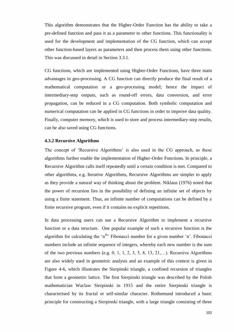
102
This algorithm demonstrates that the Higher-Order Function has the ability to take a
pre-defined function and pass it as a parameter to other functions. This functionality is
used for the development and implementation of the CG function, which can accept
other function-based layers as parameters and then process them using other functions.
This was discussed in detail in Section 3.3.1.
CG functions, which are implemented using Higher-Order Functions, have three main
advantages in geo-processing. A CG function can directly produce the final result of a
mathematical computation or a geo-processing model; hence the impact of
intermediary-step outputs, such as round-off errors, data conversion, and error
propagation, can be reduced in a CG computation. Both symbolic computation and
numerical computation can be applied in CG functions in order to improve data quality.
Finally, computer memory, which is used to store and process intermediary-step results,
can be also saved using CG functions.
4.3.2 Recursive Algorithms
The concept of ‘Recursive Algorithms’ is also used in the CG approach, as these
algorithms further enable the implementation of Higher-Order Functions. In principle, a
Recursive Algorithm calls itself repeatedly until a certain condition is met. Compared to
other algorithms, e.g. Iterative Algorithms, Recursive Algorithms are simpler to apply
as they provide a natural way of thinking about the problem. Niklaus (1976) noted that
the power of recursion lies in the possibility of defining an infinite set of objects by
using a finite statement. Thus, an infinite number of computations can be defined by a
finite recursive program, even if it contains no explicit repetitions.
In data processing users can use a Recursive Algorithm to implement a recursive
function or a data structure. One popular example of such a recursive function is the
algorithm for calculating the ‘nth
’ Fibonacci number for a given number ‘n’. Fibonacci
numbers include an infinite sequence of integers, whereby each new number is the sum
of the two previous numbers (e.g. 0, 1, 1, 2, 3, 5, 8, 13, 21,…). Recursive Algorithms
are also widely used in geometric analysis and an example of this context is given in
Figure 4-6, which illustrates the Sierpinski triangle, a confined recursion of triangles
that form a geometric lattice. The first Sierpinski triangle was described by the Polish
mathematician Waclaw Sierpinski in 1915 and the entire Sierpinski triangle is
characterised by its fractal or self-similar character. Rothemund introduced a basic
principle for constructing a Sierpinski triangle, with a large triangle consisting of three
103
smaller triangles, and each of them consisting of a further three smaller and black
triangles. This process is repeated recursively until the final Sierpinski triangle is built.
Figure 4- 6 The Sierpinski triangle (after Weisstein, 2013).
In the next section the concept of Lazy Evaluation is discussed, which is used in this
research thesis in order to run CG functions using a specific sequence of execution, i.e.
the priority-based computation strategy.
4.3.3 Lazy Evaluation
In computer science, there are two common strategies that can be used in order to
execute functions; the Eager Evaluation and Lazy Evaluation strategies. Eager
Evaluation is the most commonly used strategy and is applied by various popular
programming languages, such as C and Java. In this evaluation strategy a function is
executed once it bonds to a variable, while a Lazy Evaluation offers an alternative way
that can be used for the calculation of functions. In the Lazy Evaluation strategy
functions are only executed when the calculation needs them. As memory and time
efficiency issues are considered in the CG approach, the Lazy Evaluation strategy is
used. Lazy Evaluation enables the suspending of function-based layers and calculating
them via a specific sequence.
The use of Lazy Evaluation for the manipulation and execution of function-based layers
in the CG approach has two main advantages: Lazy Evaluation executes a function only
when it is necessary and it never performs the same step twice. To illustrate these
advantages two examples are provided below, which compare calculating the mean,
variance and standard deviation of a list of numbers, using the Eager and Lazy
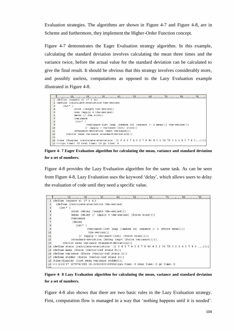
104
Evaluation strategies. The algorithms are shown in Figure 4-7 and Figure 4-8, are in
Scheme and furthermore, they implement the Higher-Order Function concept.
Figure 4-7 demonstrates the Eager Evaluation strategy algorithm. In this example,
calculating the standard deviation involves calculating the mean three times and the
variance twice, before the actual value for the standard deviation can be calculated to
give the final result. It should be obvious that this strategy involves considerably more,
and possibly useless, computations as opposed to the Lazy Evaluation example
illustrated in Figure 4-8.
Figure 4- 7 Eager Evaluation algorithm for calculating the mean, variance and standard deviation
for a set of numbers.
Figure 4-8 provides the Lazy Evaluation algorithm for the same task. As can be seen
from Figure 4-8, Lazy Evaluation uses the keyword ‘delay’, which allows users to delay
the evaluation of code until they need a specific value.
Figure 4- 8 Lazy Evaluation algorithm for calculating the mean, variance and standard deviation
for a set of numbers.
Figure 4-8 also shows that there are two basic rules in the Lazy Evaluation strategy.
First, computation flow is managed in a way that ‘nothing happens until it is needed’.
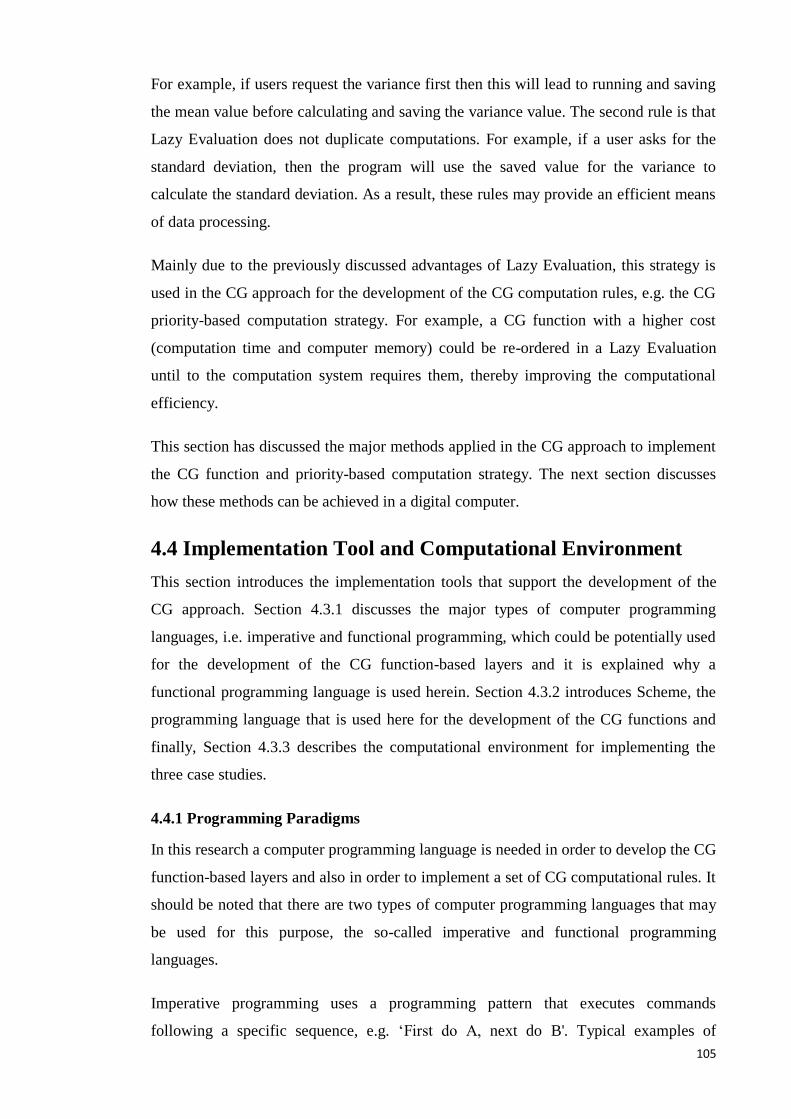
105
For example, if users request the variance first then this will lead to running and saving
the mean value before calculating and saving the variance value. The second rule is that
Lazy Evaluation does not duplicate computations. For example, if a user asks for the
standard deviation, then the program will use the saved value for the variance to
calculate the standard deviation. As a result, these rules may provide an efficient means
of data processing.
Mainly due to the previously discussed advantages of Lazy Evaluation, this strategy is
used in the CG approach for the development of the CG computation rules, e.g. the CG
priority-based computation strategy. For example, a CG function with a higher cost
(computation time and computer memory) could be re-ordered in a Lazy Evaluation
until to the computation system requires them, thereby improving the computational
efficiency.
This section has discussed the major methods applied in the CG approach to implement
the CG function and priority-based computation strategy. The next section discusses
how these methods can be achieved in a digital computer.
4.4 Implementation Tool and Computational Environment
This section introduces the implementation tools that support the development of the
CG approach. Section 4.3.1 discusses the major types of computer programming
languages, i.e. imperative and functional programming, which could be potentially used
for the development of the CG function-based layers and it is explained why a
functional programming language is used herein. Section 4.3.2 introduces Scheme, the
programming language that is used here for the development of the CG functions and
finally, Section 4.3.3 describes the computational environment for implementing the
three case studies.
4.4.1 Programming Paradigms
In this research a computer programming language is needed in order to develop the CG
function-based layers and also in order to implement a set of CG computational rules. It
should be noted that there are two types of computer programming languages that may
be used for this purpose, the so-called imperative and functional programming
languages.
Imperative programming uses a programming pattern that executes commands
following a specific sequence, e.g. ‘First do A, next do B'. Typical examples of
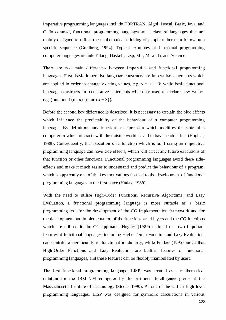
106
imperative programming languages include FORTRAN, Algol, Pascal, Basic, Java, and
C. In contrast, functional programming languages are a class of languages that are
mainly designed to reflect the mathematical thinking of people rather than following a
specific sequence (Goldberg, 1994). Typical examples of functional programming
computer languages include Erlang, Haskell, Lisp, ML, Miranda, and Scheme.
There are two main differences between imperative and functional programming
languages. First, basic imperative language constructs are imperative statements which
are applied in order to change existing values, e.g. x = x + 3; while basic functional
language constructs are declarative statements which are used to declare new values,
e.g. (function f (int x) {return x + 3}).
Before the second key difference is described, it is necessary to explain the side effects
which influence the predictability of the behaviour of a computer programming
language. By definition, any function or expression which modifies the state of a
computer or which interacts with the outside world is said to have a side effect (Hughes,
1989). Consequently, the execution of a function which is built using an imperative
programming language can have side effects, which will affect any future executions of
that function or other functions. Functional programming languages avoid these side-
effects and make it much easier to understand and predict the behaviour of a program,
which is apparently one of the key motivations that led to the development of functional
programming languages in the first place (Hudak, 1989).
With the need to utilise High-Order Functions, Recursive Algorithms, and Lazy
Evaluation, a functional programming language is more suitable as a basic
programming tool for the development of the CG implementation framework and for
the development and implementation of the function-based layers and the CG functions
which are utilised in the CG approach. Hughes (1989) claimed that two important
features of functional languages, including Higher-Order Function and Lazy Evaluation,
can contribute significantly to functional modularity, while Fokker (1995) noted that
High-Order Functions and Lazy Evaluation are built-in features of functional
programming languages, and these features can be flexibly manipulated by users.
The first functional programming language, LISP, was created as a mathematical
notation for the IBM 704 computer by the Artificial Intelligence group at the
Massachusetts Institute of Technology (Steele, 1990). As one of the earliest high-level
programming languages, LISP was designed for symbolic calculations in various
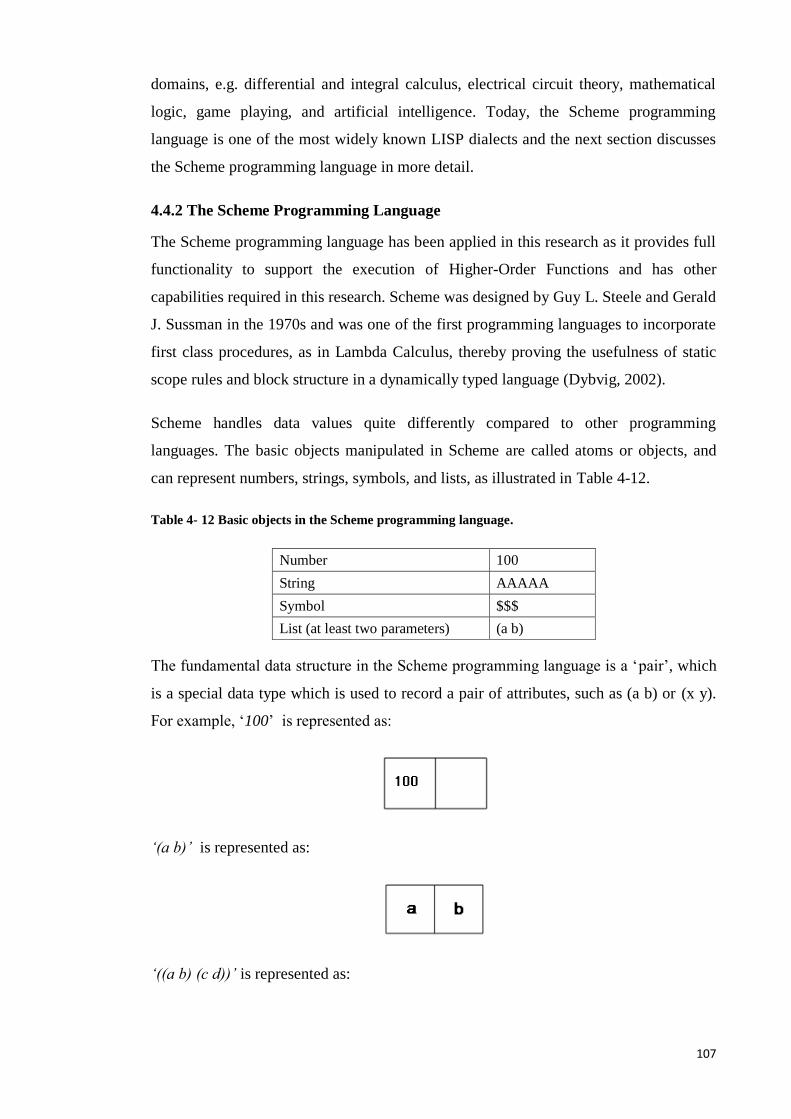
107
domains, e.g. differential and integral calculus, electrical circuit theory, mathematical
logic, game playing, and artificial intelligence. Today, the Scheme programming
language is one of the most widely known LISP dialects and the next section discusses
the Scheme programming language in more detail.
4.4.2 The Scheme Programming Language
The Scheme programming language has been applied in this research as it provides full
functionality to support the execution of Higher-Order Functions and has other
capabilities required in this research. Scheme was designed by Guy L. Steele and Gerald
J. Sussman in the 1970s and was one of the first programming languages to incorporate
first class procedures, as in Lambda Calculus, thereby proving the usefulness of static
scope rules and block structure in a dynamically typed language (Dybvig, 2002).
Scheme handles data values quite differently compared to other programming
languages. The basic objects manipulated in Scheme are called atoms or objects, and
can represent numbers, strings, symbols, and lists, as illustrated in Table 4-12.
Table 4- 12 Basic objects in the Scheme programming language.
Number 100
String AAAAA
Symbol $$$
List (at least two parameters) (a b)
The fundamental data structure in the Scheme programming language is a ‘pair’, which
is a special data type which is used to record a pair of attributes, such as (a b) or (x y).
For example, ‘100’ is represented as:
‘(a b)’ is represented as:
‘((a b) (c d))’ is represented as:
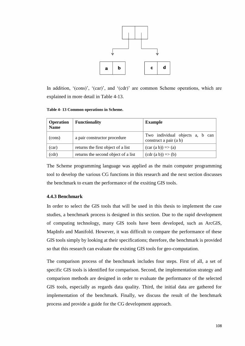
108
In addition, ‘(cons)’, ‘(car)’, and ‘(cdr)’ are common Scheme operations, which are
explained in more detail in Table 4-13.
Table 4- 13 Common operations in Scheme.
Operation
Name
Functionality Example
(cons) a pair constructor procedure Two individual objects a, b can
construct a pair (a b)
(car) returns the first object of a list (car (a b)) => (a)
(cdr) returns the second object of a list (cdr (a b)) => (b)
The Scheme programming language was applied as the main computer programming
tool to develop the various CG functions in this research and the next section discusses
the benchmark to exam the performance of the exsiting GIS tools.
4.4.3 Benchmark
In order to select the GIS tools that will be used in this thesis to implement the case
studies, a benchmark process is designed in this section. Due to the rapid development
of computing technology, many GIS tools have been developed, such as ArcGIS,
MapInfo and Manifold. However, it was difficult to compare the performance of these
GIS tools simply by looking at their specifications; therefore, the benchmark is provided
so that this research can evaluate the existing GIS tools for geo-computation.
The comparison process of the benchmark includes four steps. First of all, a set of
specific GIS tools is identified for comparison. Second, the implementation strategy and
comparison methods are designed in order to evaluate the performance of the selected
GIS tools, especially as regards data quality. Third, the initial data are gathered for
implementation of the benchmark. Finally, we discuss the result of the benchmark
process and provide a guide for the CG development approach.
109
4.4.3.1 Scope of benchmark
This section discusses the GIS tools and function which are used for the benchmark.
Four GIS tools are used (Table 4-14). ArcGIS, MapInfo and Manifold are used for this
purpose, as they are commercial GIS software packages, which are widely used by
various private and public companies for spatial analysis purposes. R, which is an open-
source statistical package with spatial analysis capabilities, is also used to validate the
computation performance in the benchmark.
The computer programmer language Python is applied in this section to produce the
reference data. The reference layer plays an important role in the benchmark, as the
various results are compared with the reference layer in order to validate the data quality
obtained using the four GIS tools.
Table 4- 14 GIS tools used for evaluating findings.
GIS tools Description
ArcGIS A desktop GIS software developed by ESRI. There are three
product levels in ArcGIS’s licences, which include
ArcReader (basic level), ArcView (middle level), and
ArcInfo (top level). ArcGIS was developed using an object-
orientation approach for storing and operating spatial
features and basic information. Currently, ArcGIS includes
several integrated applications, such as ArcMap, ArcCatalog,
ArcToolbox, ArcSence, and ArcGlobe.
MapInfo MapInfo was the first desktop GIS, developed in 1986 with
the initial aim of creating an easy-to-use GIS software. Its
major characteristics include: (a) good support for the
Microsoft operating system – Microsoft Excel®, Microsoft
Access® or database data which can be directly opened in
MapInfo; (b) MapInfo collaborated with Oracle Corporation
to develop the original spatial database, therefore, Oracle®
data can be easily accessed and viewed in MapInfo.
Manifold A low-cost GIS commercial software product.
R (R Project for R provides an open-source environment for implementing
110
Statistical Computing) many spatial analysis functions and it is assumed that more
care was paid to its implementation to ensure that it
resembles the basic equation.
The IDW function is selected in the benchmark to test the performance of the GIS tools.
This function is a commonly used spatial interpolation method, and it can be used to
assign values to unknown points by using values from a scattered set of known points
(Hengl 2009). However, the assumed value has data uncertainties which could impact
on the data quality of outputs. Therefore, the IDW function is selected in the benchmark
to compare the data quality of outputs which are produced from the selected GIS tools.
The IDW algorithm is displayed in Appendix D, which is used in Python and CG
approach to implement the IDW function. The next section introduces the
implementation strategy and the comparison methods used.
4.4.3.2 Implementation Strategy and Comparison Methods
In the benchmark process, the IDW function was implemented using the CG approach,
as well as the traditional geo-processing approach, by using the following GIS tools and
computer programming language: ArcGIS, MapInfo, Manifold, R, and Python.
Figure 4-9 illustrates the three major steps that were undertaken for the IDW
implementation. As can be seen from Figure 4-9, in the first step the points are selected
from the raw LiDAR data, and then the selected points are used to produce a sample
dataset, which includes 80% of the selected data. This sample dataset is to be used as
input data for the IDW function implementation to examine the impact of data quality
issues.
The second step mainly focuses on the generation of the sample layer by using ArcGIS,
MapInfo, Manifold, R, and the CG approach. The sample layer is the layer that is
produced after the IDW implementation and includes the interpolated values. Since five
GIS tools are used to apply the various IDW functions, the interpolated values in IDW
outputs may differ, and thus, as explained in the following sections, the results of the
various IDW implementations are further validated.
Python is used to create a reference layer for comparison. Specifically, Python is
applied to implement the same IDW algorithm, which is displayed in Appendix D, to
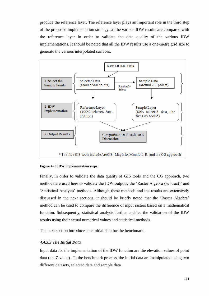
111
produce the reference layer. The reference layer plays an important role in the third step
of the proposed implementation strategy, as the various IDW results are compared with
the reference layer in order to validate the data quality of the various IDW
implementations. It should be noted that all the IDW results use a one-metre grid size to
generate the various interpolated surfaces.
Figure 4- 9 IDW implementation steps.
Finally, in order to validate the data quality of GIS tools and the CG approach, two
methods are used here to validate the IDW outputs; the ‘Raster Algebra (subtract)’ and
‘Statistical Analysis’ methods. Although these methods and the results are extensively
discussed in the next sections, it should be briefly noted that the ‘Raster Algebra’
method can be used to compare the difference of input rasters based on a mathematical
function. Subsequently, statistical analysis further enables the validation of the IDW
results using their actual numerical values and statistical methods.
The next section introduces the initial data for the benchmark.
4.4.3.3 The Initial Data
Input data for the implementation of the IDW function are the elevation values of point
data (i.e. Z value). In the benchmark process, the initial data are manipulated using two
different datasets, selected data and sample data.
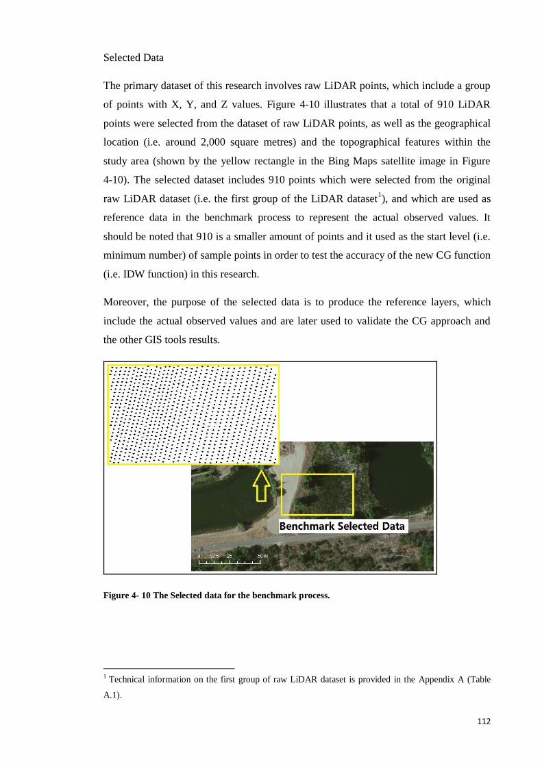
112
Selected Data
The primary dataset of this research involves raw LiDAR points, which include a group
of points with X, Y, and Z values. Figure 4-10 illustrates that a total of 910 LiDAR
points were selected from the dataset of raw LiDAR points, as well as the geographical
location (i.e. around 2,000 square metres) and the topographical features within the
study area (shown by the yellow rectangle in the Bing Maps satellite image in Figure
4-10). The selected dataset includes 910 points which were selected from the original
raw LiDAR dataset (i.e. the first group of the LiDAR dataset1), and which are used as
reference data in the benchmark process to represent the actual observed values. It
should be noted that 910 is a smaller amount of points and it used as the start level (i.e.
minimum number) of sample points in order to test the accuracy of the new CG function
(i.e. IDW function) in this research.
Moreover, the purpose of the selected data is to produce the reference layers, which
include the actual observed values and are later used to validate the CG approach and
the other GIS tools results.
Figure 4- 10 The Selected data for the benchmark process.
1 Technical information on the first group of raw LiDAR dataset is provided in the Appendix A (Table
A.1).
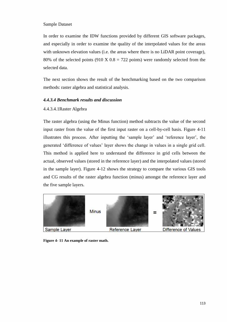
113
Sample Dataset
In order to examine the IDW functions provided by different GIS software packages,
and especially in order to examine the quality of the interpolated values for the areas
with unknown elevation values (i.e. the areas where there is no LiDAR point coverage),
80% of the selected points (910 X 0.8 = 722 points) were randomly selected from the
selected data.
The next section shows the result of the benchmarking based on the two comparison
methods: raster algebra and statistical analysis.
4.4.3.4 Benchmark results and discussion
4.4.3.4.1Raster Algebra
The raster algebra (using the Minus function) method subtracts the value of the second
input raster from the value of the first input raster on a cell-by-cell basis. Figure 4-11
illustrates this process. After inputting the ‘sample layer’ and ‘reference layer’, the
generated ‘difference of values’ layer shows the change in values in a single grid cell.
This method is applied here to understand the difference in grid cells between the
actual, observed values (stored in the reference layer) and the interpolated values (stored
in the sample layer). Figure 4-12 shows the strategy to compare the various GIS tools
and CG results of the raster algebra function (minus) amongst the reference layer and
the five sample layers.
Figure 4- 11 An example of raster math.
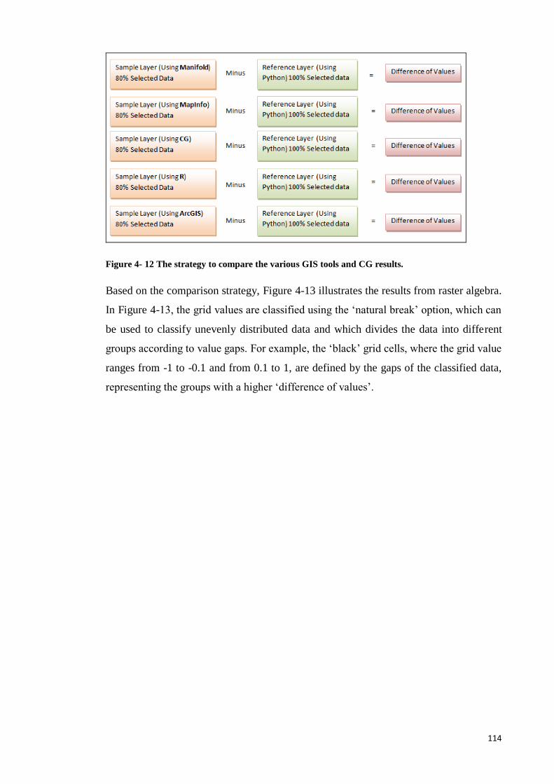
114
Figure 4- 12 The strategy to compare the various GIS tools and CG results.
Based on the comparison strategy, Figure 4-13 illustrates the results from raster algebra.
In Figure 4-13, the grid values are classified using the ‘natural break’ option, which can
be used to classify unevenly distributed data and which divides the data into different
groups according to value gaps. For example, the ‘black’ grid cells, where the grid value
ranges from -1 to -0.1 and from 0.1 to 1, are defined by the gaps of the classified data,
representing the groups with a higher ‘difference of values’.

115
Figure 4- 13 Raster algebra: Comparison of IDW outcomes.
The results of the ‘raster algebra (minus)’ operation are illustrated in Figure 4-13, and it
is noteworthy that the results generated using Manifold and MapInfo have many
differences with respect to the reference layer. At the same time the ArcGIS, R and CG
results are very similar. Therefore, a mainly descriptive-based statistical analysis was
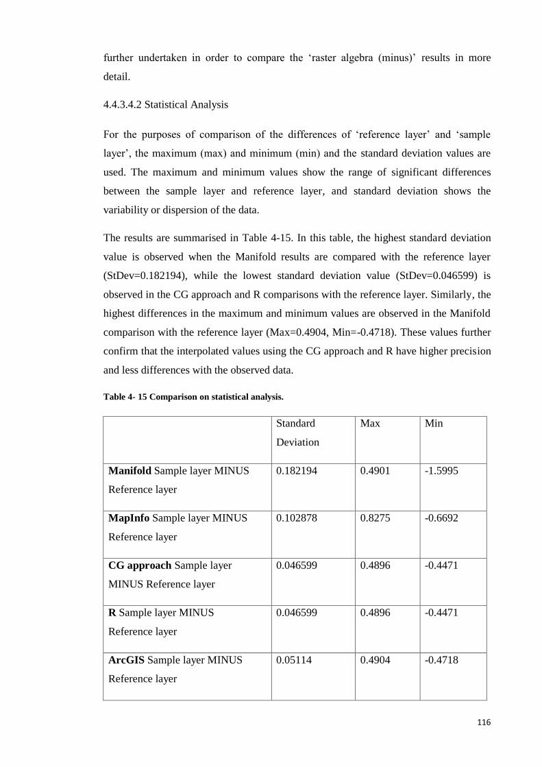
116
further undertaken in order to compare the ‘raster algebra (minus)’ results in more
detail.
4.4.3.4.2 Statistical Analysis
For the purposes of comparison of the differences of ‘reference layer’ and ‘sample
layer’, the maximum (max) and minimum (min) and the standard deviation values are
used. The maximum and minimum values show the range of significant differences
between the sample layer and reference layer, and standard deviation shows the
variability or dispersion of the data.
The results are summarised in Table 4-15. In this table, the highest standard deviation
value is observed when the Manifold results are compared with the reference layer
(StDev=0.182194), while the lowest standard deviation value (StDev=0.046599) is
observed in the CG approach and R comparisons with the reference layer. Similarly, the
highest differences in the maximum and minimum values are observed in the Manifold
comparison with the reference layer (Max=0.4904, Min=-0.4718). These values further
confirm that the interpolated values using the CG approach and R have higher precision
and less differences with the observed data.
Table 4- 15 Comparison on statistical analysis.
Standard
Deviation
Max Min
Manifold Sample layer MINUS
Reference layer
0.182194 0.4901 -1.5995
MapInfo Sample layer MINUS
Reference layer
0.102878 0.8275 -0.6692
CG approach Sample layer
MINUS Reference layer
0.046599 0.4896 -0.4471
R Sample layer MINUS
Reference layer
0.046599 0.4896 -0.4471
ArcGIS Sample layer MINUS
Reference layer
0.05114 0.4904 -0.4718
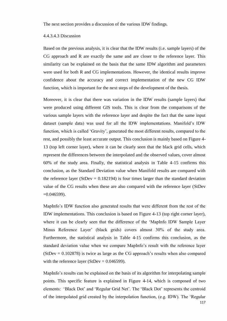
117
The next section provides a discussion of the various IDW findings.
4.4.3.4.3 Discussion
Based on the previous analysis, it is clear that the IDW results (i.e. sample layers) of the
CG approach and R are exactly the same and are closer to the reference layer. This
similarity can be explained on the basis that the same IDW algorithm and parameters
were used for both R and CG implementations. However, the identical results improve
confidence about the accuracy and correct implementation of the new CG IDW
function, which is important for the next steps of the development of the thesis.
Moreover, it is clear that there was variation in the IDW results (sample layers) that
were produced using different GIS tools. This is clear from the comparisons of the
various sample layers with the reference layer and despite the fact that the same input
dataset (sample data) was used for all the IDW implementations. Manifold’s IDW
function, which is called ‘Gravity’, generated the most different results, compared to the
rest, and possibly the least accurate output. This conclusion is mainly based on Figure 4-
13 (top left corner layer), where it can be clearly seen that the black grid cells, which
represent the differences between the interpolated and the observed values, cover almost
60% of the study area. Finally, the statistical analysis in Table 4-15 confirms this
conclusion, as the Standard Deviation value when Manifold results are compared with
the reference layer (StDev = 0.182194) is four times larger than the standard deviation
value of the CG results when these are also compared with the reference layer (StDev
=0.046599).
MapInfo’s IDW function also generated results that were different from the rest of the
IDW implementations. This conclusion is based on Figure 4-13 (top right corner layer),
where it can be clearly seen that the difference of the ‘MapInfo IDW Sample Layer
Minus Reference Layer’ (black grids) covers almost 30% of the study area.
Furthermore, the statistical analysis in Table 4-15 confirms this conclusion, as the
standard deviation value when we compare MapInfo’s result with the reference layer
(StDev = 0.102878) is twice as large as the CG approach’s results when also compared
with the reference layer (StDev = 0.046599).
MapInfo’s results can be explained on the basis of its algorithm for interpolating sample
points. This specific feature is explained in Figure 4-14, which is composed of two
elements: ‘Black Dot’ and ‘Regular Grid Net’. The ‘Black Dot’ represents the centroid
of the interpolated grid created by the interpolation function, (e.g. IDW). The ‘Regular
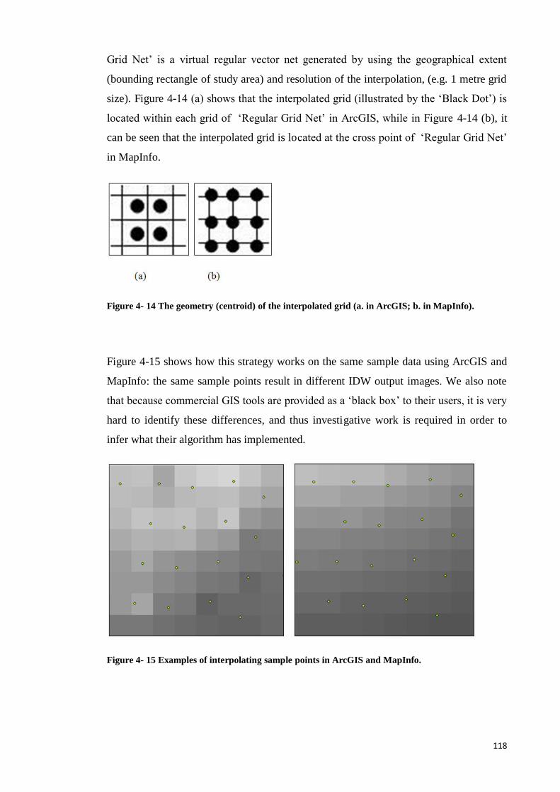
118
Grid Net’ is a virtual regular vector net generated by using the geographical extent
(bounding rectangle of study area) and resolution of the interpolation, (e.g. 1 metre grid
size). Figure 4-14 (a) shows that the interpolated grid (illustrated by the ‘Black Dot’) is
located within each grid of ‘Regular Grid Net’ in ArcGIS, while in Figure 4-14 (b), it
can be seen that the interpolated grid is located at the cross point of ‘Regular Grid Net’
in MapInfo.
Figure 4- 14 The geometry (centroid) of the interpolated grid (a. in ArcGIS; b. in MapInfo).
Figure 4-15 shows how this strategy works on the same sample data using ArcGIS and
MapInfo: the same sample points result in different IDW output images. We also note
that because commercial GIS tools are provided as a ‘black box’ to their users, it is very
hard to identify these differences, and thus investigative work is required in order to
infer what their algorithm has implemented.
Figure 4- 15 Examples of interpolating sample points in ArcGIS and MapInfo.
119
Compared with Manifold and MapInfo, ArcGIS, the CG approach and R provided the
most accurate results. In Figure 4-13, it is difficult to identify the differences between
the results between these three GIS tools. However, based on the statistical analysis, we
observe that the CG approach and R are slightly more accurate than ArcGIS. For
instance, Table 4-15 reveals that the Standard Deviation value from the comparison of
the CG approach and R results and the reference layer (StDev = 0.046599) is 20% better
than the comparison of the ArcGIS result and the reference layer (StDev = 0.05114).
In conclusion, this benchmark process has demonstrated the performance of the selected
GIS tools. Specifically, the results of the different IDW implementations were
compared and it was found that the CG IDW implementation results were very similar
to the IDW implementation results using R, while the interpolated results using the CG
approach and R had the smallest standard deviation value. Thus, the CG approach has
many potential advantages, especially when dealing with simple raster data (e.g. the
interpolated values using the CG IDW function are closer to the observed values).
Moreover, ArcGIS provides a better performance than other commercial GIS tools (e.g.
MapInfo and Manifold) based on the ‘raster algebra (subtract)’ and ‘statistical analysis’
comparison results. Therefore, the CG approach and ArcGIS are used as the two major
GIS tools in the following case studies.
Moreover, it should be noted that R will be not used in the case studies, although it
produced the same output with the CG approach in the benchmark. That is because R
provides fewer spatial analysis functions, compared with ArcGIS and MapInfo.
The next section discusses the computational environment for the case studies.
4.4.4 Computational Environment
This section introduces the computational environment for the three case studies,
including both the traditional geo-processing approach (Section 4.4.3.1) and the CG
approach (Section 4.4.3.2). The computational environment is defined as a summary of
the features of the software packages and the computer for implementing the three case
studies in this thesis.
4.4.4.1 The Traditional Geo-processing Approach
There are two GIS tools that were used in this thesis to implement the case studies using
the traditional geo-processing approach: ArcGIS Version 9.2 (Figure 4-16) and MapInfo
120
Version 8.5.1 (Figure 4-17). ArcGIS and MapInfo are common commercial GIS
software packages, which are widely used for spatial analysis purposes.
Figure 4- 16 ArcGIS 9.2 software.
Figure 4- 17 MapInfo 8.5.1 software.
4.4.4.2 The CG Approach
As described in the previous section, the Scheme programming language was used to
create the computer programs that perform the computations in the CG approach. In this
research, the Scheme programming language was implemented using a software tool,
named Racket Version 6.1.0 (Figure 4-18). Racket, formerly named PLT Scheme, is a
full-spectrum programming language in the Lisp/Scheme family. In fact, it goes beyond
the computer programming of Lisp and Scheme, through dialects that support objects,
types, laziness, and more. One of Racket’s design goals is to serve as a platform for
language creation, design, and implementation (Figure 4-19).
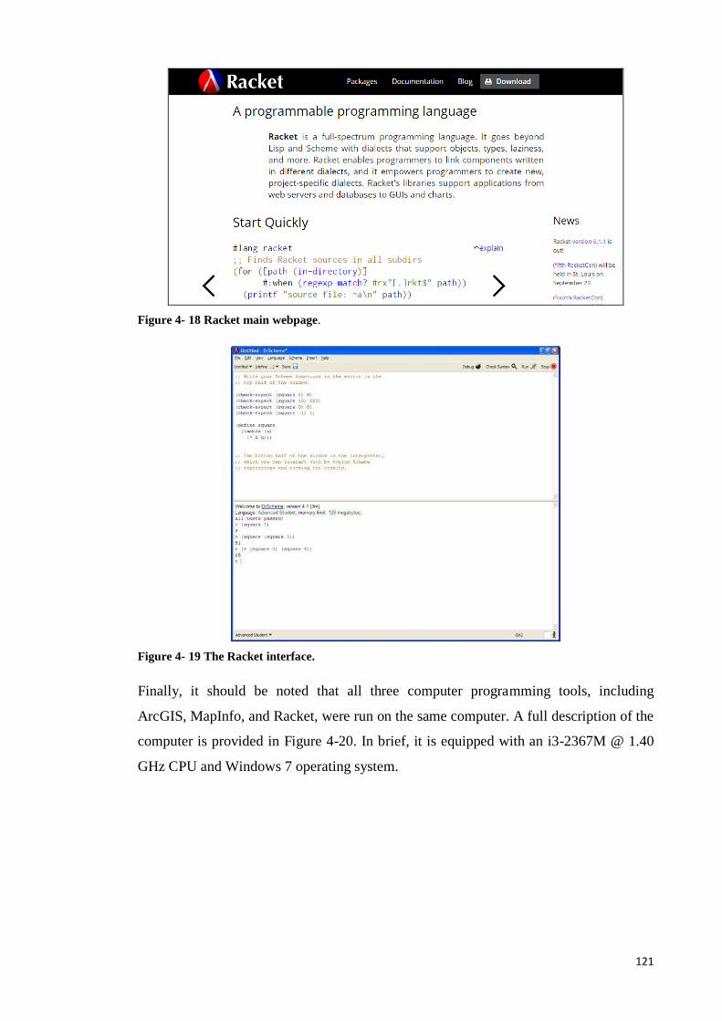
121
Figure 4- 18 Racket main webpage.
Figure 4- 19 The Racket interface.
Finally, it should be noted that all three computer programming tools, including
ArcGIS, MapInfo, and Racket, were run on the same computer. A full description of the
computer is provided in Figure 4-20. In brief, it is equipped with an i3-2367M @ 1.40
GHz CPU and Windows 7 operating system.
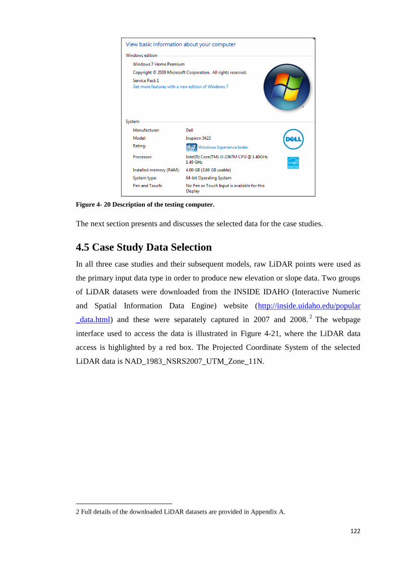
122
Figure 4- 20 Description of the testing computer.
The next section presents and discusses the selected data for the case studies.
4.5 Case Study Data Selection
In all three case studies and their subsequent models, raw LiDAR points were used as
the primary input data type in order to produce new elevation or slope data. Two groups
of LiDAR datasets were downloaded from the INSIDE IDAHO (Interactive Numeric
and Spatial Information Data Engine) website (http://inside.uidaho.edu/popular
_data.html) and these were separately captured in 2007 and 2008.2 The webpage
interface used to access the data is illustrated in Figure 4-21, where the LiDAR data
access is highlighted by a red box. The Projected Coordinate System of the selected
LiDAR data is NAD_1983_NSRS2007_UTM_Zone_11N.
2 Full details of the downloaded LiDAR datasets are provided in Appendix A.
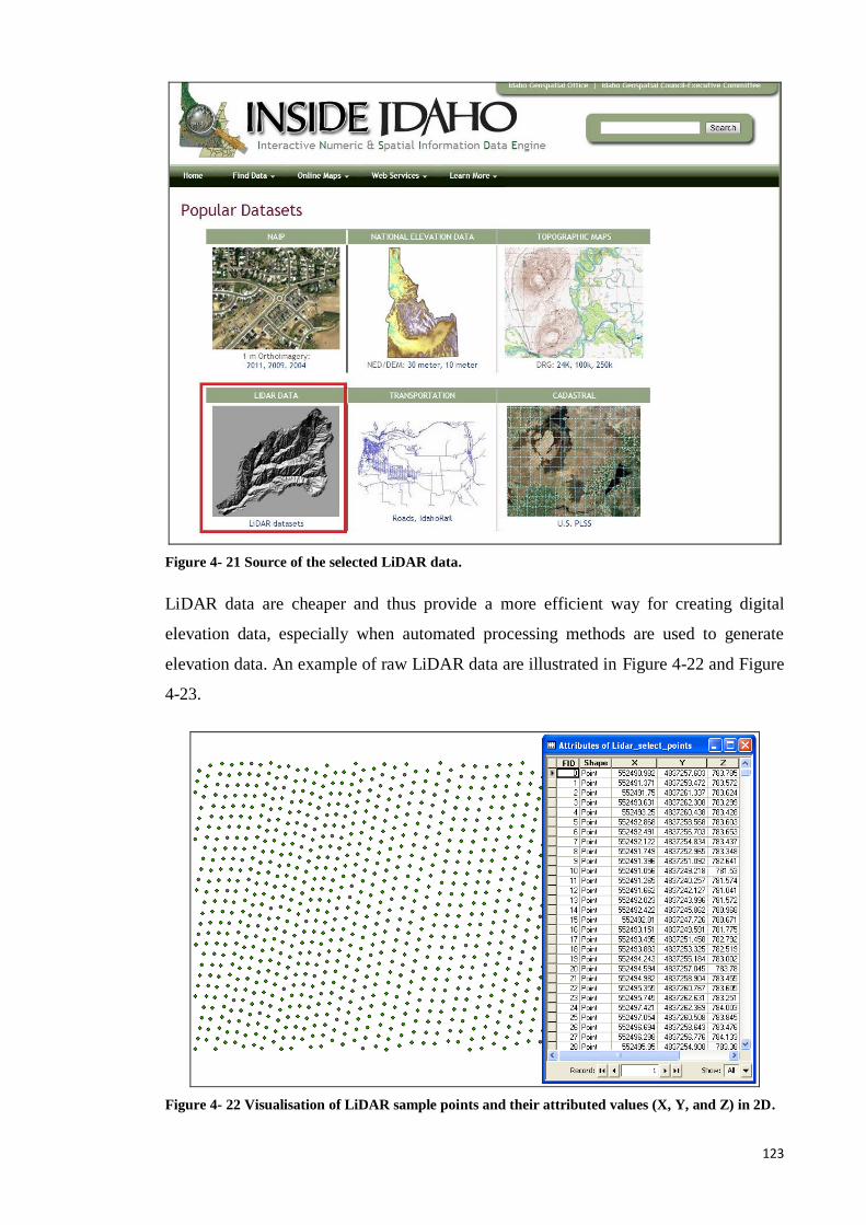
123
Figure 4- 21 Source of the selected LiDAR data.
LiDAR data are cheaper and thus provide a more efficient way for creating digital
elevation data, especially when automated processing methods are used to generate
elevation data. An example of raw LiDAR data are illustrated in Figure 4-22 and Figure
4-23.
Figure 4- 22 Visualisation of LiDAR sample points and their attributed values (X, Y, and Z) in 2D.
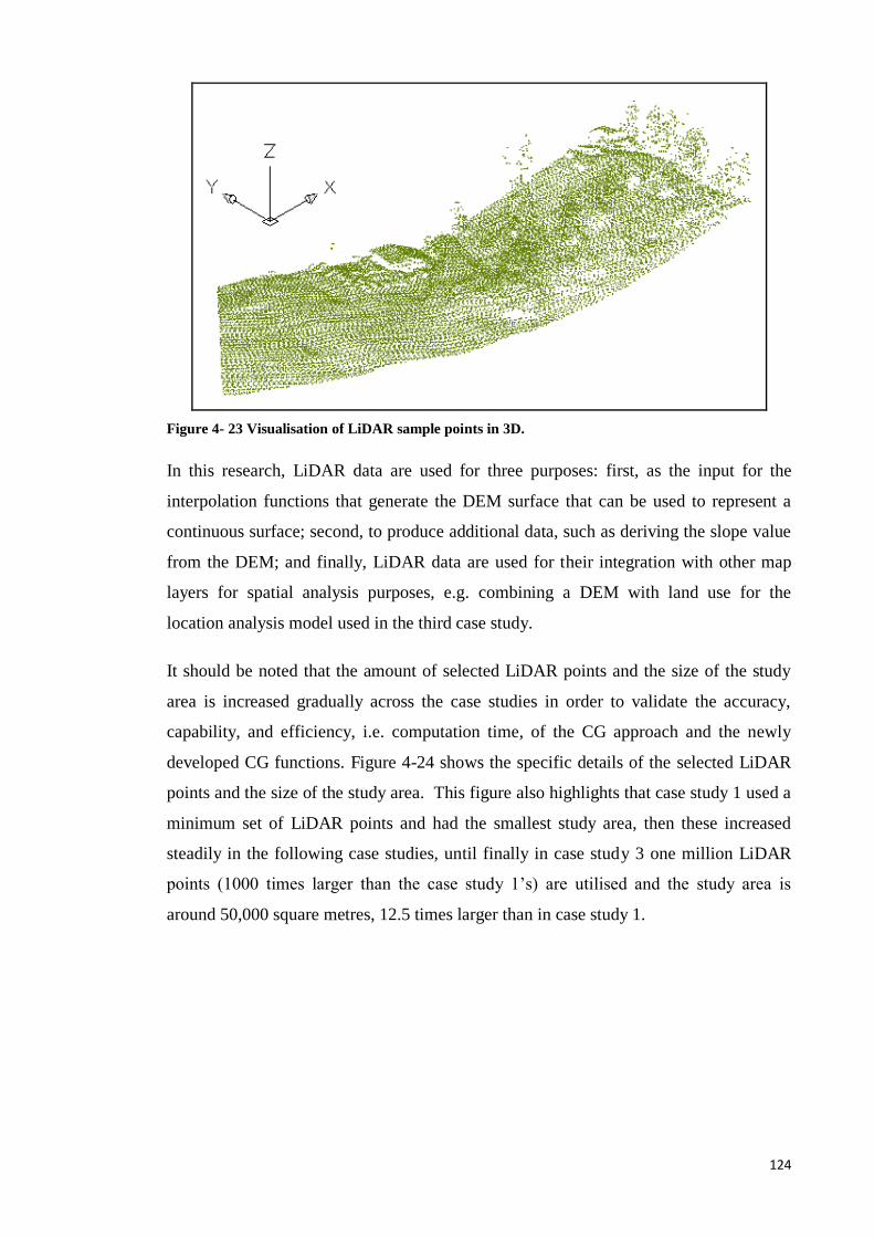
124
Figure 4- 23 Visualisation of LiDAR sample points in 3D.
In this research, LiDAR data are used for three purposes: first, as the input for the
interpolation functions that generate the DEM surface that can be used to represent a
continuous surface; second, to produce additional data, such as deriving the slope value
from the DEM; and finally, LiDAR data are used for their integration with other map
layers for spatial analysis purposes, e.g. combining a DEM with land use for the
location analysis model used in the third case study.
It should be noted that the amount of selected LiDAR points and the size of the study
area is increased gradually across the case studies in order to validate the accuracy,
capability, and efficiency, i.e. computation time, of the CG approach and the newly
developed CG functions. Figure 4-24 shows the specific details of the selected LiDAR
points and the size of the study area. This figure also highlights that case study 1 used a
minimum set of LiDAR points and had the smallest study area, then these increased
steadily in the following case studies, until finally in case study 3 one million LiDAR
points (1000 times larger than the case study 1’s) are utilised and the study area is
around 50,000 square metres, 12.5 times larger than in case study 1.
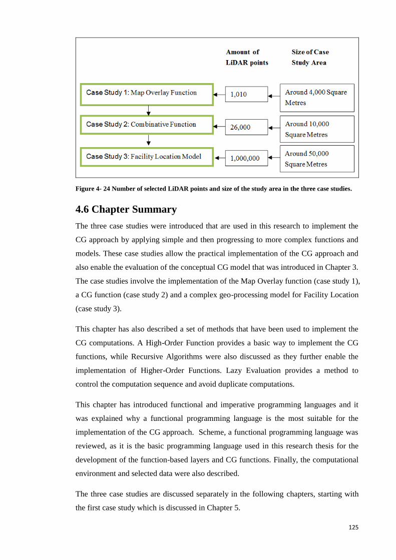
125
Figure 4- 24 Number of selected LiDAR points and size of the study area in the three case studies.
4.6 Chapter Summary
The three case studies were introduced that are used in this research to implement the
CG approach by applying simple and then progressing to more complex functions and
models. These case studies allow the practical implementation of the CG approach and
also enable the evaluation of the conceptual CG model that was introduced in Chapter 3.
The case studies involve the implementation of the Map Overlay function (case study 1),
a CG function (case study 2) and a complex geo-processing model for Facility Location
(case study 3).
This chapter has also described a set of methods that have been used to implement the
CG computations. A High-Order Function provides a basic way to implement the CG
functions, while Recursive Algorithms were also discussed as they further enable the
implementation of Higher-Order Functions. Lazy Evaluation provides a method to
control the computation sequence and avoid duplicate computations.
This chapter has introduced functional and imperative programming languages and it
was explained why a functional programming language is the most suitable for the
implementation of the CG approach. Scheme, a functional programming language was
reviewed, as it is the basic programming language used in this research thesis for the
development of the function-based layers and CG functions. Finally, the computational
environment and selected data were also described.
The three case studies are discussed separately in the following chapters, starting with
the first case study which is discussed in Chapter 5.
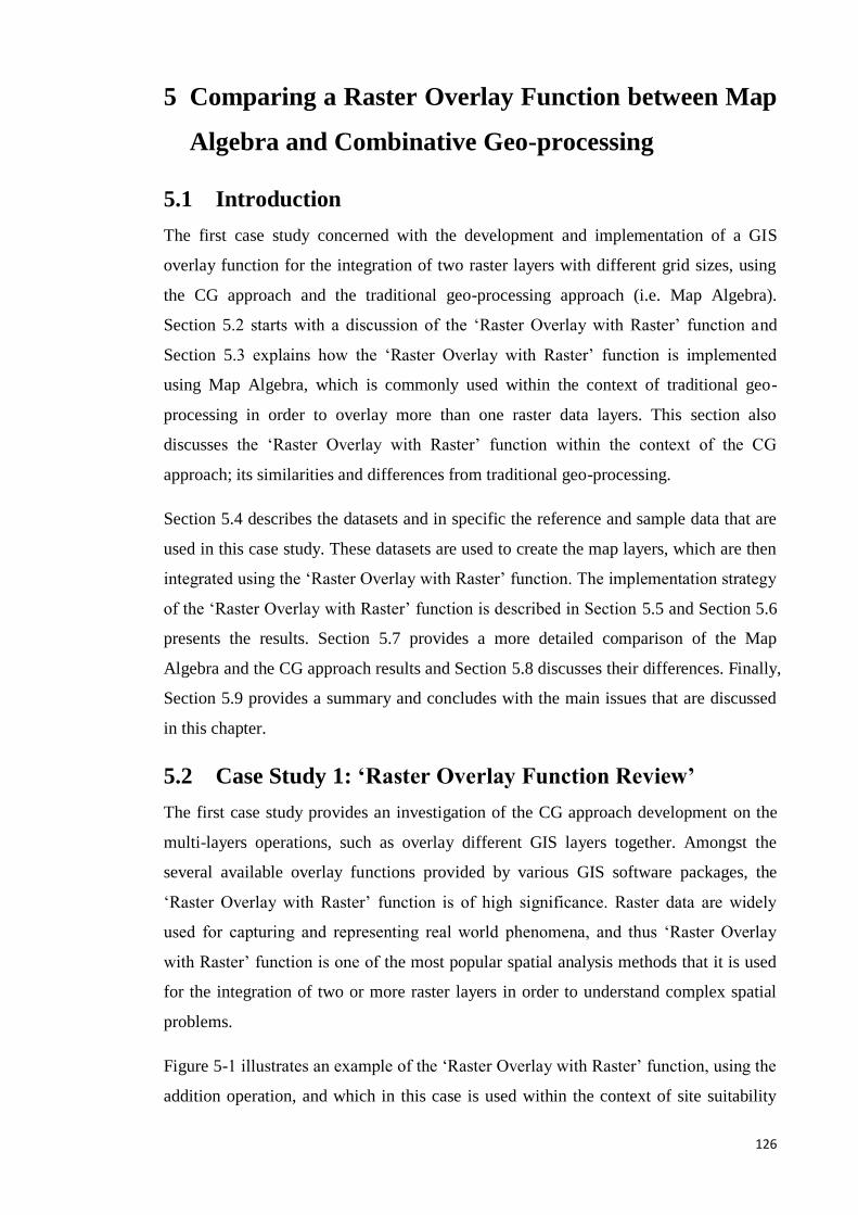
126
5 Comparing a Raster Overlay Function between Map
Algebra and Combinative Geo-processing
5.1 Introduction
The first case study concerned with the development and implementation of a GIS
overlay function for the integration of two raster layers with different grid sizes, using
the CG approach and the traditional geo-processing approach (i.e. Map Algebra).
Section 5.2 starts with a discussion of the ‘Raster Overlay with Raster’ function and
Section 5.3 explains how the ‘Raster Overlay with Raster’ function is implemented
using Map Algebra, which is commonly used within the context of traditional geo-
processing in order to overlay more than one raster data layers. This section also
discusses the ‘Raster Overlay with Raster’ function within the context of the CG
approach; its similarities and differences from traditional geo-processing.
Section 5.4 describes the datasets and in specific the reference and sample data that are
used in this case study. These datasets are used to create the map layers, which are then
integrated using the ‘Raster Overlay with Raster’ function. The implementation strategy
of the ‘Raster Overlay with Raster’ function is described in Section 5.5 and Section 5.6
presents the results. Section 5.7 provides a more detailed comparison of the Map
Algebra and the CG approach results and Section 5.8 discusses their differences. Finally,
Section 5.9 provides a summary and concludes with the main issues that are discussed
in this chapter.
5.2 Case Study 1: ‘Raster Overlay Function Review’
The first case study provides an investigation of the CG approach development on the
multi-layers operations, such as overlay different GIS layers together. Amongst the
several available overlay functions provided by various GIS software packages, the
‘Raster Overlay with Raster’ function is of high significance. Raster data are widely
used for capturing and representing real world phenomena, and thus ‘Raster Overlay
with Raster’ function is one of the most popular spatial analysis methods that it is used
for the integration of two or more raster layers in order to understand complex spatial
problems.
Figure 5-1 illustrates an example of the ‘Raster Overlay with Raster’ function, using the
addition operation, and which in this case is used within the context of site suitability
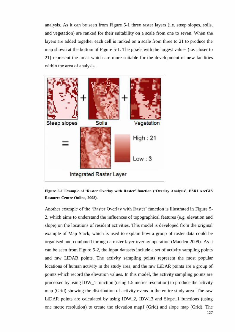
127
analysis. As it can be seen from Figure 5-1 three raster layers (i.e. steep slopes, soils,
and vegetation) are ranked for their suitability on a scale from one to seven. When the
layers are added together each cell is ranked on a scale from three to 21 to produce the
map shown at the bottom of Figure 5-1. The pixels with the largest values (i.e. closer to
21) represent the areas which are more suitable for the development of new facilities
within the area of analysis.
Figure 5-1 Example of ‘Raster Overlay with Raster’ function (‘Overlay Analysis’, ESRI ArcGIS
Resource Centre Online, 2008).
Another example of the ‘Raster Overlay with Raster’ function is illustrated in Figure 5-
2, which aims to understand the influences of topographical features (e.g. elevation and
slope) on the locations of resident activities. This model is developed from the original
example of Map Stack, which is used to explain how a group of raster data could be
organised and combined through a raster layer overlay operation (Madden 2009). As it
can be seen from Figure 5-2, the input datasets include a set of activity sampling points
and raw LiDAR points. The activity sampling points represent the most popular
locations of human activity in the study area, and the raw LiDAR points are a group of
points which record the elevation values. In this model, the activity sampling points are
processed by using IDW_1 function (using 1.5 metres resolution) to produce the activity
map (Grid) showing the distribution of activity evens in the entire study area. The raw
LiDAR points are calculated by using IDW_2, IDW_3 and Slope_1 functions (using
one metre resolution) to create the elevation map1 (Grid) and slope map (Grid). The
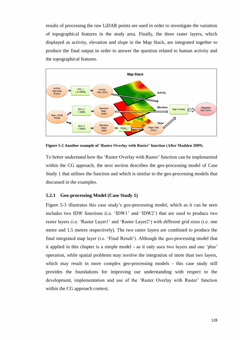
128
results of processing the raw LiDAR points are used in order to investigate the variation
of topographical features in the study area. Finally, the three raster layers, which
displayed as activity, elevation and slope in the Map Stack, are integrated together to
produce the final output in order to answer the question related to human activity and
the topographical features.
Figure 5-2 Another example of ‘Raster Overlay with Raster’ function (After Madden 2009).
To better understand how the ‘Raster Overlay with Raster’ function can be implemented
within the CG approach, the next section describes the geo-processing model of Case
Study 1 that utilises the function and which is similar to the geo-processing models that
discussed in the examples.
5.2.1 Geo-processing Model (Case Study 1)
Figure 5-3 illustrates this case study’s geo-processing model, which as it can be seen
includes two IDW functions (i.e. ‘IDW1’ and ‘IDW2’) that are used to produce two
raster layers (i.e. ‘Raster Layer1’ and ‘Raster Layer2’) with different grid sizes (i.e. one
metre and 1.5 metres respectively). The two raster layers are combined to produce the
final integrated map layer (i.e. ‘Final Result’). Although the geo-processing model that
it applied in this chapter is a simple model - as it only uses two layers and one ‘plus’
operation, while spatial problems may involve the integration of more than two layers,
which may result in more complex geo-processing models - this case study still
provides the foundations for improving our understanding with respect to the
development, implementation and use of the ‘Raster Overlay with Raster’ function
within the CG approach context.
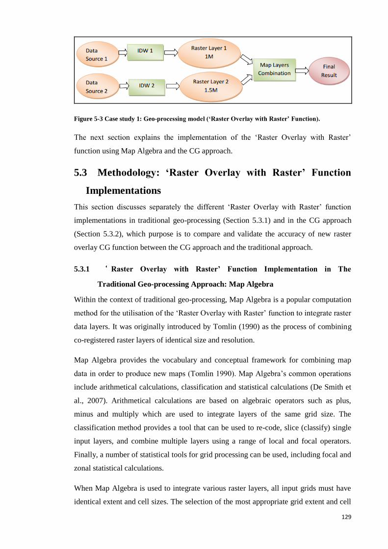
129
Figure 5-3 Case study 1: Geo-processing model (‘Raster Overlay with Raster’ Function).
The next section explains the implementation of the ‘Raster Overlay with Raster’
function using Map Algebra and the CG approach.
5.3 Methodology: ‘Raster Overlay with Raster’ Function
Implementations
This section discusses separately the different ‘Raster Overlay with Raster’ function
implementations in traditional geo-processing (Section 5.3.1) and in the CG approach
(Section 5.3.2), which purpose is to compare and validate the accuracy of new raster
overlay CG function between the CG approach and the traditional approach.
5.3.1 ‘ Raster Overlay with Raster’ Function Implementation in The
Traditional Geo-processing Approach: Map Algebra
Within the context of traditional geo-processing, Map Algebra is a popular computation
method for the utilisation of the ‘Raster Overlay with Raster’ function to integrate raster
data layers. It was originally introduced by Tomlin (1990) as the process of combining
co-registered raster layers of identical size and resolution.
Map Algebra provides the vocabulary and conceptual framework for combining map
data in order to produce new maps (Tomlin 1990). Map Algebra’s common operations
include arithmetical calculations, classification and statistical calculations (De Smith et
al., 2007). Arithmetical calculations are based on algebraic operators such as plus,
minus and multiply which are used to integrate layers of the same grid size. The
classification method provides a tool that can be used to re-code, slice (classify) single
input layers, and combine multiple layers using a range of local and focal operators.
Finally, a number of statistical tools for grid processing can be used, including focal and
zonal statistical calculations.
When Map Algebra is used to integrate various raster layers, all input grids must have
identical extent and cell sizes. The selection of the most appropriate grid extent and cell
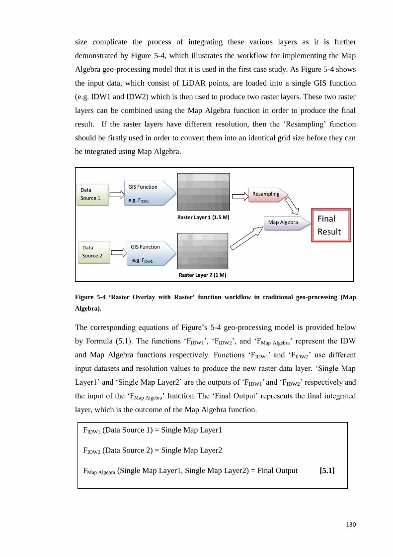
130
size complicate the process of integrating these various layers as it is further
demonstrated by Figure 5-4, which illustrates the workflow for implementing the Map
Algebra geo-processing model that it is used in the first case study. As Figure 5-4 shows
the input data, which consist of LiDAR points, are loaded into a single GIS function
(e.g. IDW1 and IDW2) which is then used to produce two raster layers. These two raster
layers can be combined using the Map Algebra function in order to produce the final
result. If the raster layers have different resolution, then the ‘Resampling’ function
should be firstly used in order to convert them into an identical grid size before they can
be integrated using Map Algebra.
Figure 5-4 ‘Raster Overlay with Raster’ function workflow in traditional geo-processing (Map
Algebra).
The corresponding equations of Figure’s 5-4 geo-processing model is provided below
by Formula (5.1). The functions ‘FIDW1’, ‘FIDW2’, and ‘FMap Algebra’ represent the IDW
and Map Algebra functions respectively. Functions ‘FIDW1’ and ‘FIDW2’ use different
input datasets and resolution values to produce the new raster data layer. ‘Single Map
Layer1’ and ‘Single Map Layer2’ are the outputs of ‘FIDW1’ and ‘FIDW2’ respectively and
the input of the ‘FMap Algebra’ function. The ‘Final Output’ represents the final integrated
layer, which is the outcome of the Map Algebra function.
FIDW1 (Data Source 1) = Single Map Layer1
FIDW2 (Data Source 2) = Single Map Layer2
FMap Algebra (Single Map Layer1, Single Map Layer2) = Final Output [5.1]
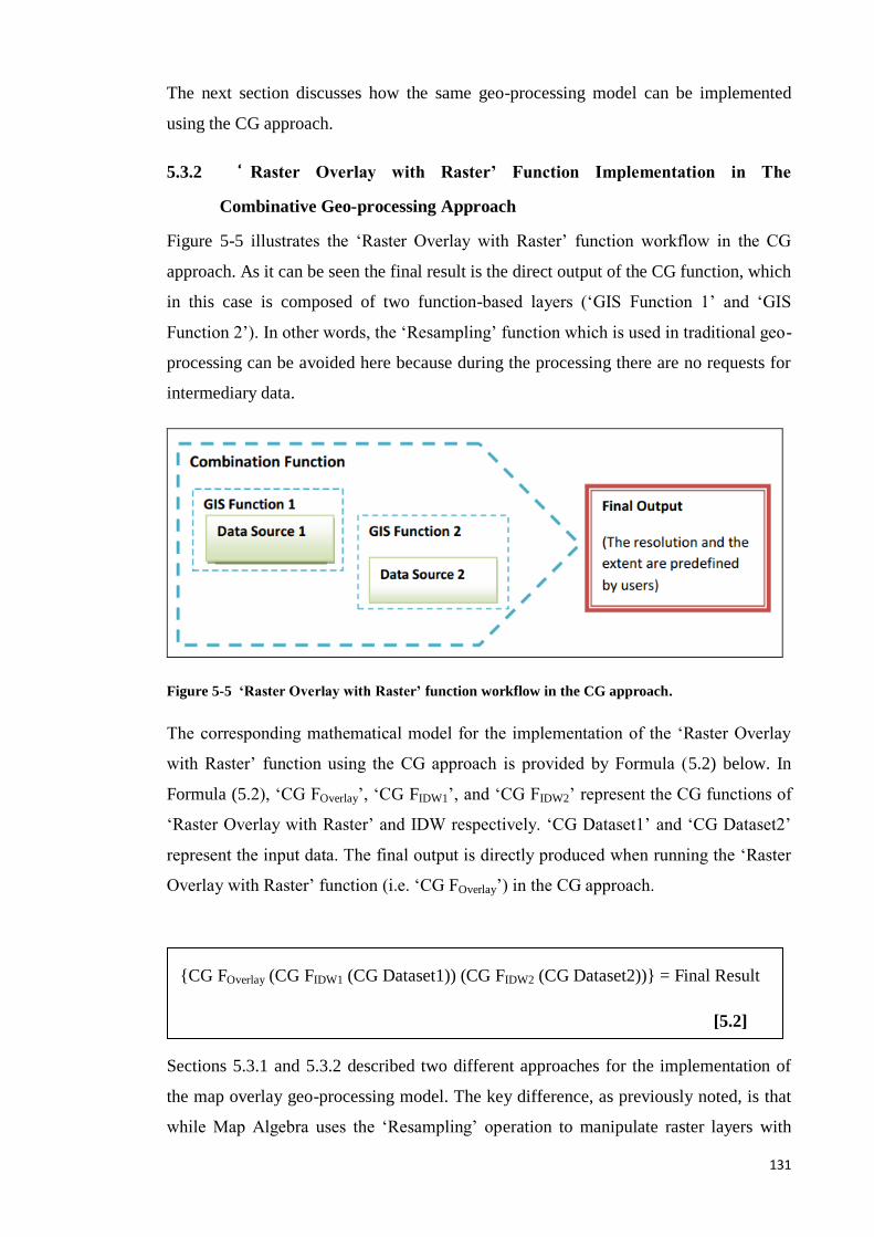
131
The next section discusses how the same geo-processing model can be implemented
using the CG approach.
5.3.2 ‘ Raster Overlay with Raster’ Function Implementation in The
Combinative Geo-processing Approach
Figure 5-5 illustrates the ‘Raster Overlay with Raster’ function workflow in the CG
approach. As it can be seen the final result is the direct output of the CG function, which
in this case is composed of two function-based layers (‘GIS Function 1’ and ‘GIS
Function 2’). In other words, the ‘Resampling’ function which is used in traditional geo-
processing can be avoided here because during the processing there are no requests for
intermediary data.
Figure 5-5 ‘Raster Overlay with Raster’ function workflow in the CG approach.
The corresponding mathematical model for the implementation of the ‘Raster Overlay
with Raster’ function using the CG approach is provided by Formula (5.2) below. In
Formula (5.2), ‘CG FOverlay’, ‘CG FIDW1’, and ‘CG FIDW2’ represent the CG functions of
‘Raster Overlay with Raster’ and IDW respectively. ‘CG Dataset1’ and ‘CG Dataset2’
represent the input data. The final output is directly produced when running the ‘Raster
Overlay with Raster’ function (i.e. ‘CG FOverlay’) in the CG approach.
{CG FOverlay (CG FIDW1 (CG Dataset1)) (CG FIDW2 (CG Dataset2))} = Final Result
[5.2]
Sections 5.3.1 and 5.3.2 described two different approaches for the implementation of
the map overlay geo-processing model. The key difference, as previously noted, is that
while Map Algebra uses the ‘Resampling’ operation to manipulate raster layers with
132
different resolutions, this step is completely avoided when using the CG approach. The
next Section (5.4) discusses the datasets that are used in the first case study.
5.4 Case study 1: ‘Raster Overlay with Raster’ Function
Implementation Datasets
The input dataset that is used in this case study to implement the ‘Raster Overlay with
Raster’ function consists of LiDAR points. Raw LiDAR points are manipulated in two
different datasets, to produce the reference and sample data, which are discussed
separately in Sections 5.4.1 and 5.4.2.
5.4.1 Reference data
Figure 5-6 illustrates a total of 1010 LiDAR points were selected from a dataset of raw
LiDAR points, as well as, the geographical location (i.e. around 4,000 square metres)
and the topographical features within the study area (shown by the yellow rectangle in
Bing Maps satellite image in Figure 5-6). The sample dataset includes 1010 points that
were selected from the original raw LiDAR dataset (i.e. the first group of the LiDAR
dataset3), and which are used as reference data in this case study to represent the actual
observed values. Moreover, the purpose of the reference data is to produce the reference
layers, which include the actual observed values and are later used to validate the CG
approach and Map Algebra results.
3 Technical information of the first group of raw LiDAR dataset is provided in the Appendix A (Table
A.1).
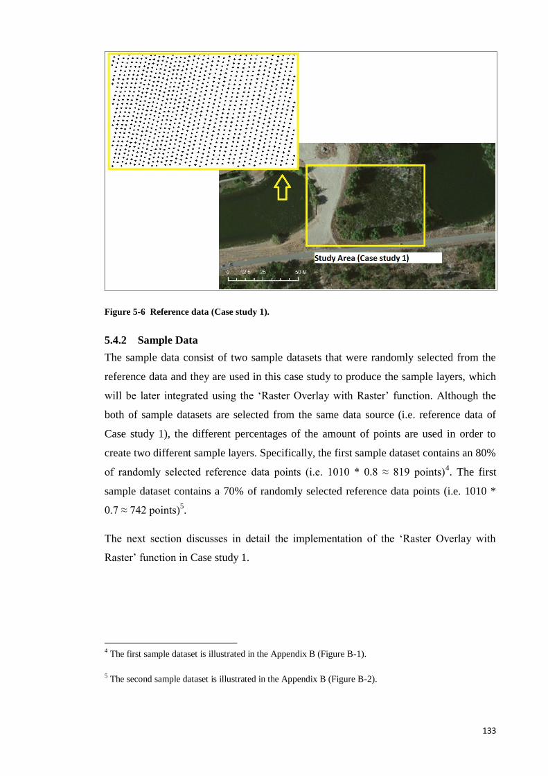
133
Figure 5-6 Reference data (Case study 1).
5.4.2 Sample Data
The sample data consist of two sample datasets that were randomly selected from the
reference data and they are used in this case study to produce the sample layers, which
will be later integrated using the ‘Raster Overlay with Raster’ function. Although the
both of sample datasets are selected from the same data source (i.e. reference data of
Case study 1), the different percentages of the amount of points are used in order to
create two different sample layers. Specifically, the first sample dataset contains an 80%
of randomly selected reference data points (i.e. 1010 * 0.8 ≈ 819 points)4. The first
sample dataset contains a 70% of randomly selected reference data points (i.e. 1010 *
0.7 ≈ 742 points)5.
The next section discusses in detail the implementation of the ‘Raster Overlay with
Raster’ function in Case study 1.
4 The first sample dataset is illustrated in the Appendix B (Figure B-1).
5 The second sample dataset is illustrated in the Appendix B (Figure B-2).
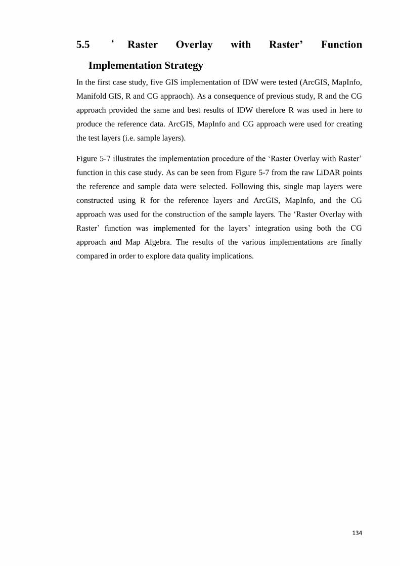
134
5.5 ‘ Raster Overlay with Raster’ Function
Implementation Strategy
In the first case study, five GIS implementation of IDW were tested (ArcGIS, MapInfo,
Manifold GIS, R and CG appraoch). As a consequence of previous study, R and the CG
approach provided the same and best results of IDW therefore R was used in here to
produce the reference data. ArcGIS, MapInfo and CG approach were used for creating
the test layers (i.e. sample layers).
Figure 5-7 illustrates the implementation procedure of the ‘Raster Overlay with Raster’
function in this case study. As can be seen from Figure 5-7 from the raw LiDAR points
the reference and sample data were selected. Following this, single map layers were
constructed using R for the reference layers and ArcGIS, MapInfo, and the CG
approach was used for the construction of the sample layers. The ‘Raster Overlay with
Raster’ function was implemented for the layers’ integration using both the CG
approach and Map Algebra. The results of the various implementations are finally
compared in order to explore data quality implications.
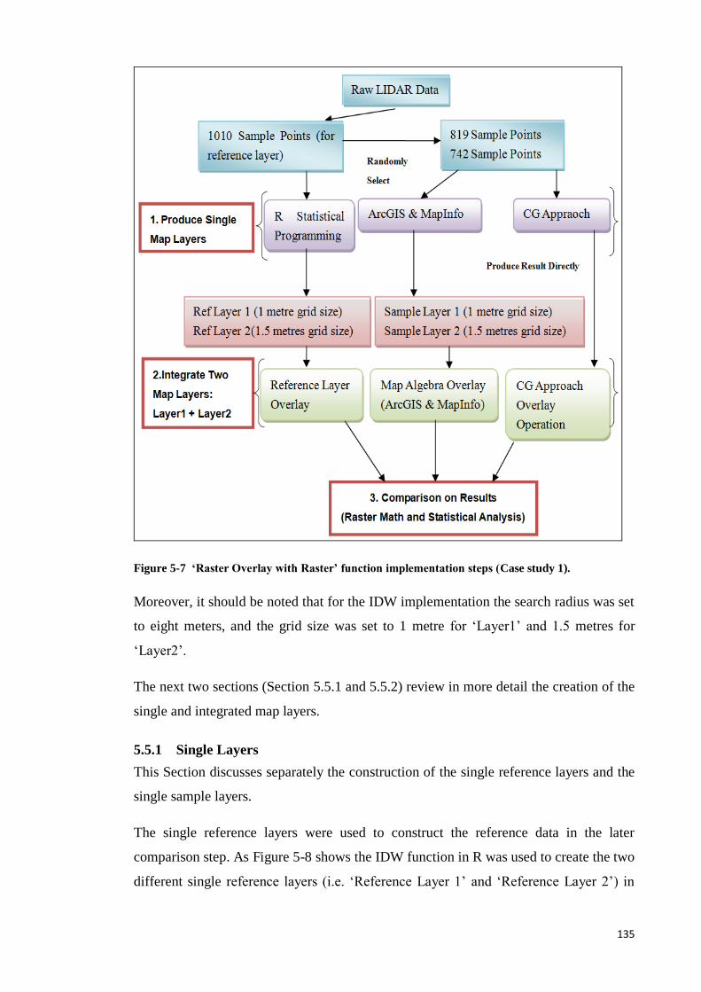
135
Figure 5-7 ‘Raster Overlay with Raster’ function implementation steps (Case study 1).
Moreover, it should be noted that for the IDW implementation the search radius was set
to eight meters, and the grid size was set to 1 metre for ‘Layer1’ and 1.5 metres for
‘Layer2’.
The next two sections (Section 5.5.1 and 5.5.2) review in more detail the creation of the
single and integrated map layers.
5.5.1 Single Layers
This Section discusses separately the construction of the single reference layers and the
single sample layers.
The single reference layers were used to construct the reference data in the later
comparison step. As Figure 5-8 shows the IDW function in R was used to create the two
different single reference layers (i.e. ‘Reference Layer 1’ and ‘Reference Layer 2’) in
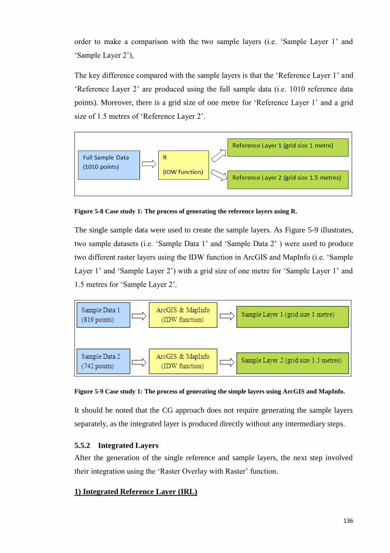
136
order to make a comparison with the two sample layers (i.e. ‘Sample Layer 1’ and
‘Sample Layer 2’),
The key difference compared with the sample layers is that the ‘Reference Layer 1’ and
‘Reference Layer 2’ are produced using the full sample data (i.e. 1010 reference data
points). Moreover, there is a grid size of one metre for ‘Reference Layer 1’ and a grid
size of 1.5 metres of ‘Reference Layer 2’.
Figure 5-8 Case study 1: The process of generating the reference layers using R.
The single sample data were used to create the sample layers. As Figure 5-9 illustrates,
two sample datasets (i.e. ‘Sample Data 1’ and ‘Sample Data 2’ ) were used to produce
two different raster layers using the IDW function in ArcGIS and MapInfo (i.e. ‘Sample
Layer 1’ and ‘Sample Layer 2’) with a grid size of one metre for ‘Sample Layer 1’ and
1.5 metres for ‘Sample Layer 2’.
Figure 5-9 Case study 1: The process of generating the simple layers using ArcGIS and MapInfo.
It should be noted that the CG approach does not require generating the sample layers
separately, as the integrated layer is produced directly without any intermediary steps.
5.5.2 Integrated Layers
After the generation of the single reference and sample layers, the next step involved
their integration using the ‘Raster Overlay with Raster’ function.
1) Integrated Reference Layer (IRL)
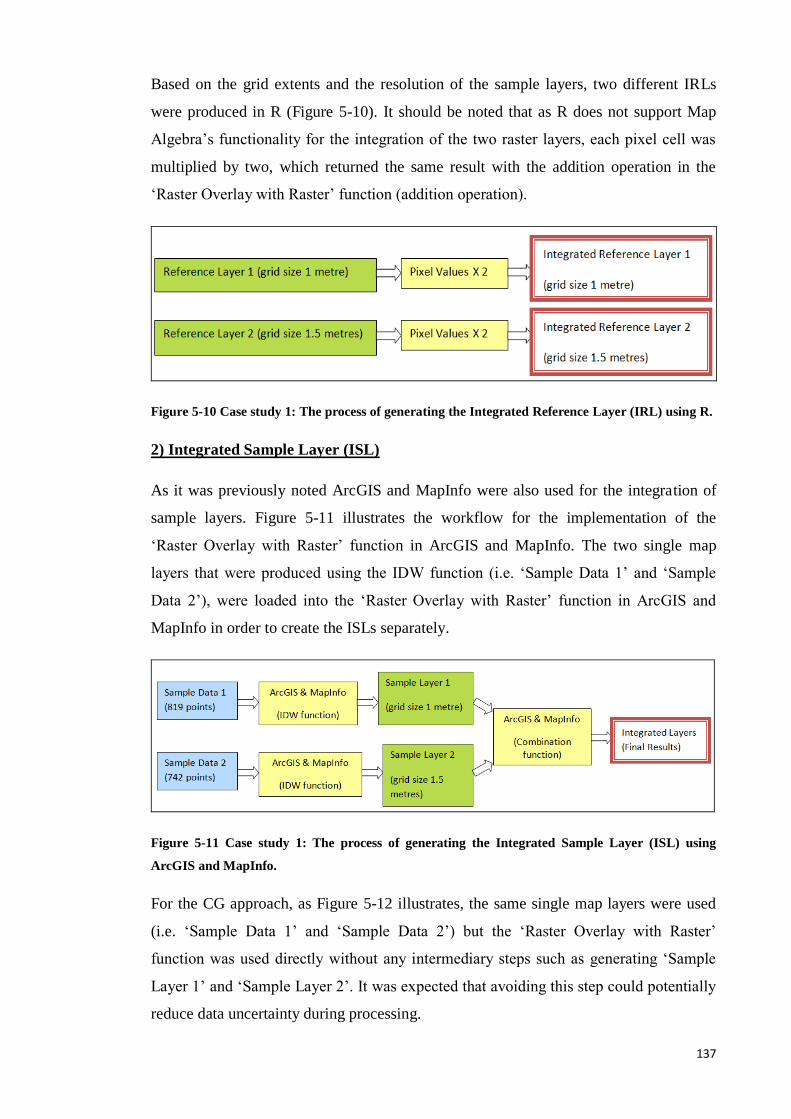
137
Based on the grid extents and the resolution of the sample layers, two different IRLs
were produced in R (Figure 5-10). It should be noted that as R does not support Map
Algebra’s functionality for the integration of the two raster layers, each pixel cell was
multiplied by two, which returned the same result with the addition operation in the
‘Raster Overlay with Raster’ function (addition operation).
Figure 5-10 Case study 1: The process of generating the Integrated Reference Layer (IRL) using R.
2) Integrated Sample Layer (ISL)
As it was previously noted ArcGIS and MapInfo were also used for the integration of
sample layers. Figure 5-11 illustrates the workflow for the implementation of the
‘Raster Overlay with Raster’ function in ArcGIS and MapInfo. The two single map
layers that were produced using the IDW function (i.e. ‘Sample Data 1’ and ‘Sample
Data 2’), were loaded into the ‘Raster Overlay with Raster’ function in ArcGIS and
MapInfo in order to create the ISLs separately.
Figure 5-11 Case study 1: The process of generating the Integrated Sample Layer (ISL) using
ArcGIS and MapInfo.
For the CG approach, as Figure 5-12 illustrates, the same single map layers were used
(i.e. ‘Sample Data 1’ and ‘Sample Data 2’) but the ‘Raster Overlay with Raster’
function was used directly without any intermediary steps such as generating ‘Sample
Layer 1’ and ‘Sample Layer 2’. It was expected that avoiding this step could potentially
reduce data uncertainty during processing.
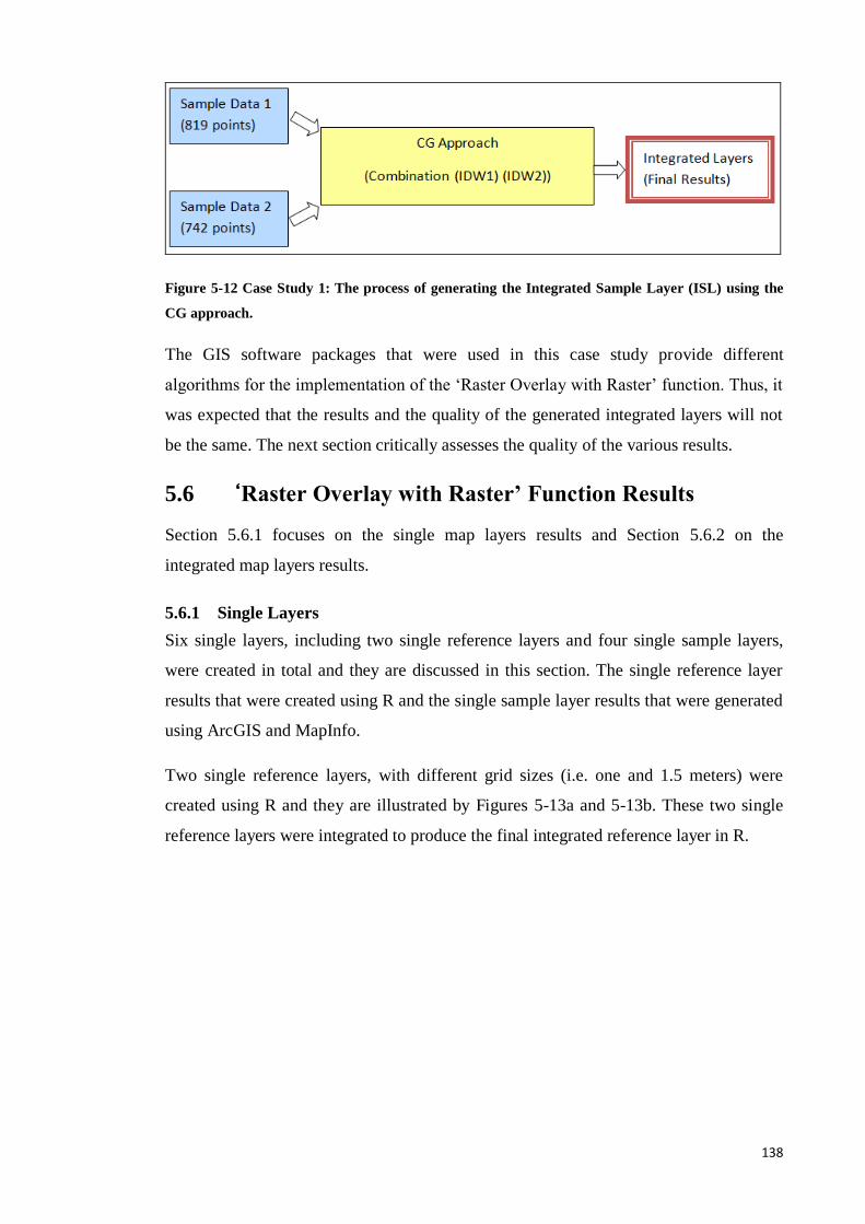
138
Figure 5-12 Case Study 1: The process of generating the Integrated Sample Layer (ISL) using the
CG approach.
The GIS software packages that were used in this case study provide different
algorithms for the implementation of the ‘Raster Overlay with Raster’ function. Thus, it
was expected that the results and the quality of the generated integrated layers will not
be the same. The next section critically assesses the quality of the various results.
5.6 ‘Raster Overlay with Raster’ Function Results
Section 5.6.1 focuses on the single map layers results and Section 5.6.2 on the
integrated map layers results.
5.6.1 Single Layers
Six single layers, including two single reference layers and four single sample layers,
were created in total and they are discussed in this section. The single reference layer
results that were created using R and the single sample layer results that were generated
using ArcGIS and MapInfo.
Two single reference layers, with different grid sizes (i.e. one and 1.5 meters) were
created using R and they are illustrated by Figures 5-13a and 5-13b. These two single
reference layers were integrated to produce the final integrated reference layer in R.
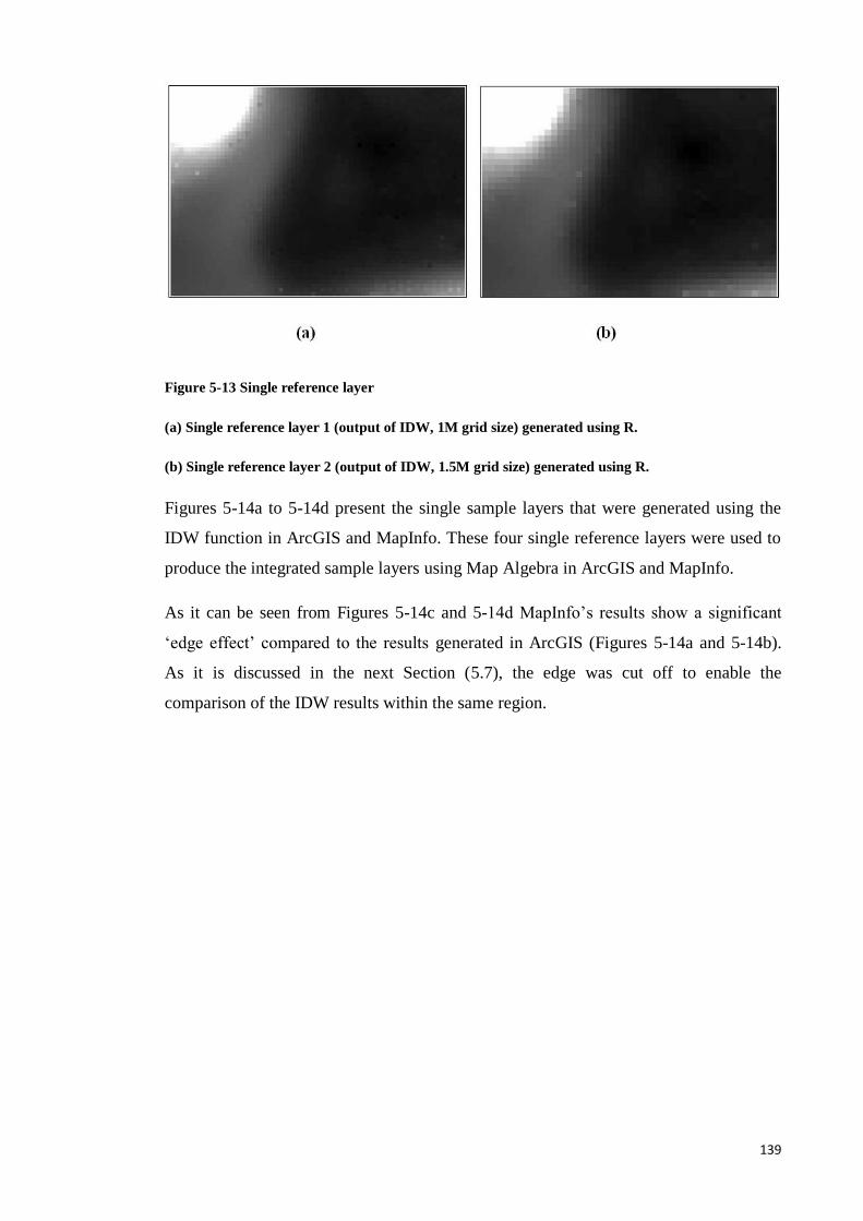
139
Figure 5-13 Single reference layer
(a) Single reference layer 1 (output of IDW, 1M grid size) generated using R.
(b) Single reference layer 2 (output of IDW, 1.5M grid size) generated using R.
Figures 5-14a to 5-14d present the single sample layers that were generated using the
IDW function in ArcGIS and MapInfo. These four single reference layers were used to
produce the integrated sample layers using Map Algebra in ArcGIS and MapInfo.
As it can be seen from Figures 5-14c and 5-14d MapInfo’s results show a significant
‘edge effect’ compared to the results generated in ArcGIS (Figures 5-14a and 5-14b).
As it is discussed in the next Section (5.7), the edge was cut off to enable the
comparison of the IDW results within the same region.
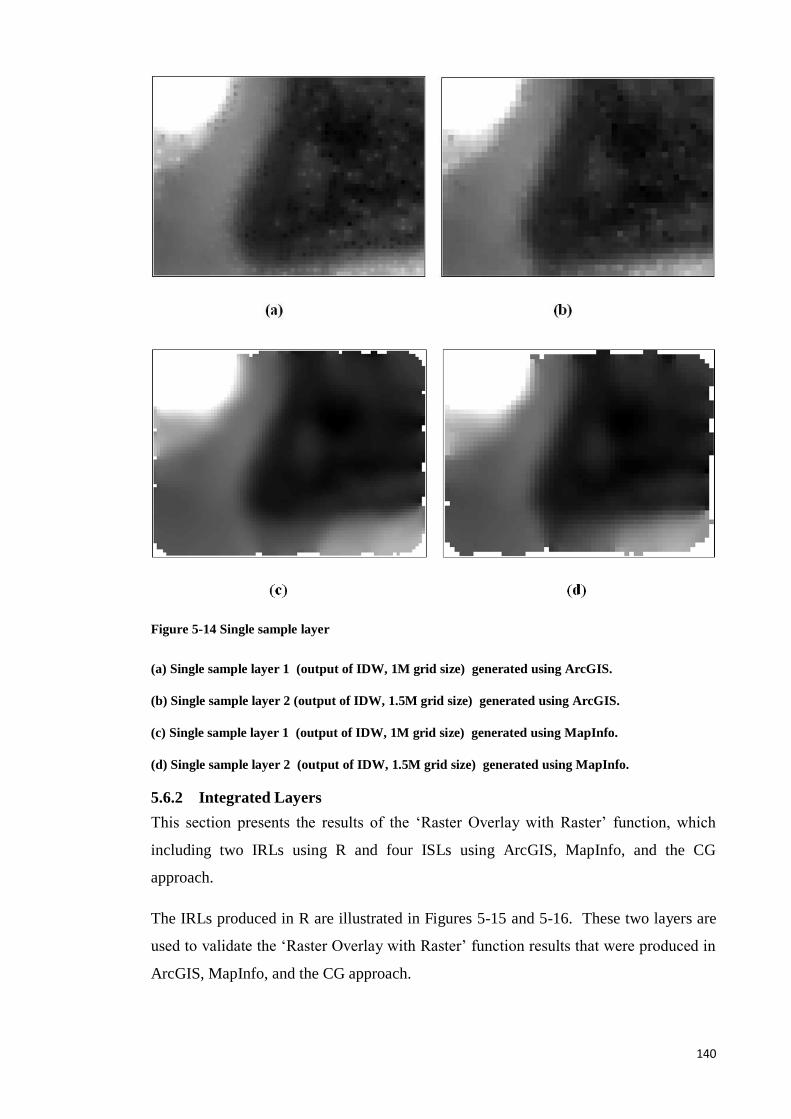
140
Figure 5-14 Single sample layer
(a) Single sample layer 1 (output of IDW, 1M grid size) generated using ArcGIS.
(b) Single sample layer 2 (output of IDW, 1.5M grid size) generated using ArcGIS.
(c) Single sample layer 1 (output of IDW, 1M grid size) generated using MapInfo.
(d) Single sample layer 2 (output of IDW, 1.5M grid size) generated using MapInfo.
5.6.2 Integrated Layers
This section presents the results of the ‘Raster Overlay with Raster’ function, which
including two IRLs using R and four ISLs using ArcGIS, MapInfo, and the CG
approach.
The IRLs produced in R are illustrated in Figures 5-15 and 5-16. These two layers are
used to validate the ‘Raster Overlay with Raster’ function results that were produced in
ArcGIS, MapInfo, and the CG approach.
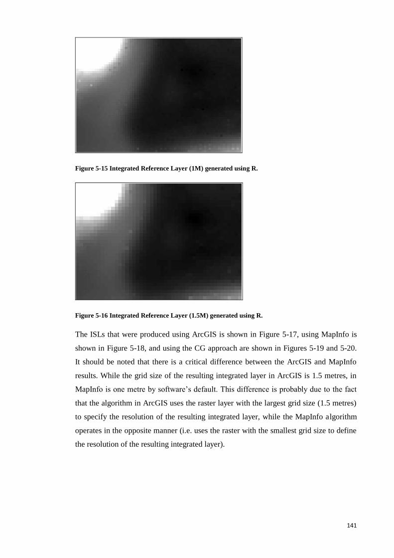
141
Figure 5-15 Integrated Reference Layer (1M) generated using R.
Figure 5-16 Integrated Reference Layer (1.5M) generated using R.
The ISLs that were produced using ArcGIS is shown in Figure 5-17, using MapInfo is
shown in Figure 5-18, and using the CG approach are shown in Figures 5-19 and 5-20.
It should be noted that there is a critical difference between the ArcGIS and MapInfo
results. While the grid size of the resulting integrated layer in ArcGIS is 1.5 metres, in
MapInfo is one metre by software’s default. This difference is probably due to the fact
that the algorithm in ArcGIS uses the raster layer with the largest grid size (1.5 metres)
to specify the resolution of the resulting integrated layer, while the MapInfo algorithm
operates in the opposite manner (i.e. uses the raster with the smallest grid size to define
the resolution of the resulting integrated layer).
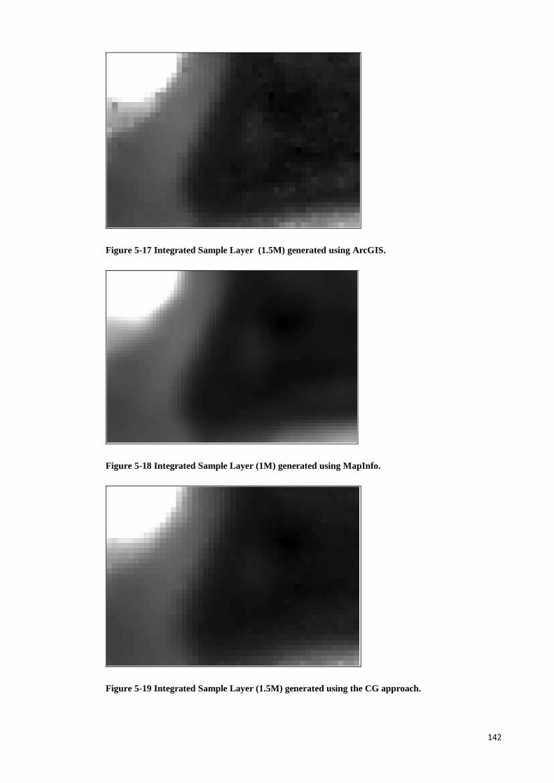
142
Figure 5-17 Integrated Sample Layer (1.5M) generated using ArcGIS.
Figure 5-18 Integrated Sample Layer (1M) generated using MapInfo.
Figure 5-19 Integrated Sample Layer (1.5M) generated using the CG approach.
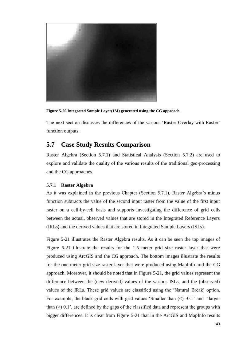
143
Figure 5-20 Integrated Sample Layer(1M) generated using the CG approach.
The next section discusses the differences of the various ‘Raster Overlay with Raster’
function outputs.
5.7 Case Study Results Comparison
Raster Algebra (Section 5.7.1) and Statistical Analysis (Section 5.7.2) are used to
explore and validate the quality of the various results of the traditional geo-processing
and the CG approaches.
5.7.1 Raster Algebra
As it was explained in the previous Chapter (Section 5.7.1), Raster Algebra’s minus
function subtracts the value of the second input raster from the value of the first input
raster on a cell-by-cell basis and supports investigating the difference of grid cells
between the actual, observed values that are stored in the Integrated Reference Layers
(IRLs) and the derived values that are stored in Integrated Sample Layers (ISLs).
Figure 5-21 illustrates the Raster Algebra results. As it can be seen the top images of
Figure 5-21 illustrate the results for the 1.5 meter grid size raster layer that were
produced using ArcGIS and the CG approach. The bottom images illustrate the results
for the one meter grid size raster layer that were produced using MapInfo and the CG
approach. Moreover, it should be noted that in Figure 5-21, the grid values represent the
difference between the (new derived) values of the various ISLs, and the (observed)
values of the IRLs. These grid values are classified using the ‘Natural Break’ option.
For example, the black grid cells with grid values ‘Smaller than (<) -0.1’ and ‘larger
than (>) 0.1’, are defined by the gaps of the classified data and represent the groups with
bigger differences. It is clear from Figure 5-21 that in the ArcGIS and MapInfo results
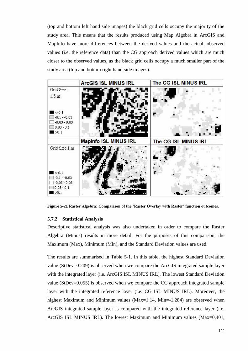
144
(top and bottom left hand side images) the black grid cells occupy the majority of the
study area. This means that the results produced using Map Algebra in ArcGIS and
MapInfo have more differences between the derived values and the actual, observed
values (i.e. the reference data) than the CG approach derived values which are much
closer to the observed values, as the black grid cells occupy a much smaller part of the
study area (top and bottom right hand side images).
Figure 5-21 Raster Algebra: Comparison of the ‘Raster Overlay with Raster’ function outcomes.
5.7.2 Statistical Analysis
Descriptive statistical analysis was also undertaken in order to compare the Raster
Algebra (Minus) results in more detail. For the purposes of this comparison, the
Maximum (Max), Minimum (Min), and the Standard Deviation values are used.
The results are summarised in Table 5-1. In this table, the highest Standard Deviation
value (StDev=0.209) is observed when we compare the ArcGIS integrated sample layer
with the integrated layer (i.e. ArcGIS ISL MINUS IRL). The lowest Standard Deviation
value (StDev=0.055) is observed when we compare the CG approach integrated sample
layer with the integrated reference layer (i.e. CG ISL MINUS IRL). Moreover, the
highest Maximum and Minimum values (Max=1.14, Min=-1.284) are observed when
ArcGIS integrated sample layer is compared with the integrated reference layer (i.e.
ArcGIS ISL MINUS IRL). The lowest Maximum and Minimum values (Max=0.401,
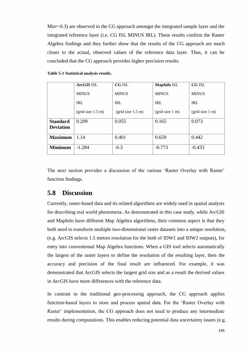
145
Min=-0.3) are observed in the CG approach amongst the integrated sample layer and the
integrated reference layer (i.e. CG ISL MINUS IRL). These results confirm the Raster
Algebra findings and they further show that the results of the CG approach are much
closer to the actual, observed values of the reference data layer. Thus, it can be
concluded that the CG approach provides higher precision results.
Table 5-1 Statistical analysis results.
ArcGIS ISL
MINUS
IRL
(grid size 1.5 m)
CG ISL
MINUS
IRL
(grid size 1.5 m)
MapInfo ISL
MINUS
IRL
(grid size 1 m)
CG ISL
MINUS
IRL
(grid size 1 m)
Standard
Deviation
0.209 0.055 0.165 0.073
Maximum 1.14 0.401 0.659 0.442
Minimum -1.284 -0.3 -0.773 -0.433
The next section provides a discussion of the various ‘Raster Overlay with Raster’
function findings.
5.8 Discussion
Currently, raster-based data and its related algorithms are widely used in spatial analysis
for describing real world phenomena. As demonstrated in this case study, while ArcGIS
and MapInfo have different Map Algebra algorithms, their common aspect is that they
both need to transform multiple two-dimensional raster datasets into a unique resolution,
(e.g. ArcGIS selects 1.5 metres resolution for the both of IDW1 and IDW2 outputs), for
entry into conventional Map Algebra functions. When a GIS tool selects automatically
the largest of the raster layers to define the resolution of the resulting layer, then the
accuracy and precision of the final result are influenced. For example, it was
demonstrated that ArcGIS selects the largest grid size and as a result the derived values
in ArcGIS have more differences with the reference data.
In contrast to the traditional geo-processing approach, the CG approach applies
function-based layers to store and process spatial data. For the ‘Raster Overlay with
Raster’ implementation, the CG approach does not need to produce any intermediate
results during computations. This enables reducing potential data uncertainty issues (e.g.
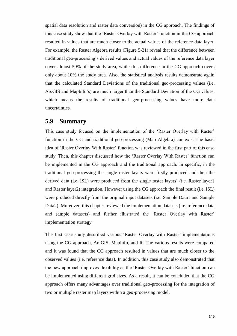
146
spatial data resolution and raster data conversion) in the CG approach. The findings of
this case study show that the ‘Raster Overlay with Raster’ function in the CG approach
resulted in values that are much closer to the actual values of the reference data layer.
For example, the Raster Algebra results (Figure 5-21) reveal that the difference between
traditional geo-processing’s derived values and actual values of the reference data layer
cover almost 50% of the study area, while this difference in the CG approach covers
only about 10% the study area. Also, the statistical analysis results demonstrate again
that the calculated Standard Deviations of the traditional geo-processing values (i.e.
ArcGIS and MapInfo’s) are much larger than the Standard Deviation of the CG values,
which means the results of traditional geo-processing values have more data
uncertainties.
5.9 Summary
This case study focused on the implementation of the ‘Raster Overlay with Raster’
function in the CG and traditional geo-processing (Map Algebra) contexts. The basic
idea of ‘Raster Overlay With Raster’ function was reviewed in the first part of this case
study. Then, this chapter discussed how the ‘Raster Overlay With Raster’ function can
be implemented in the CG approach and the traditional approach. In specific, in the
traditional geo-processing the single raster layers were firstly produced and then the
derived data (i.e. ISL) were produced from the single raster layers’ (i.e. Raster layer1
and Raster layer2) integration. However using the CG approach the final result (i.e. ISL)
were produced directly from the original input datasets (i.e. Sample Data1 and Sample
Data2). Moreover, this chapter reviewed the implementation datasets (i.e. reference data
and sample datasets) and further illustrated the ‘Raster Overlay with Raster’
implementation strategy.
The first case study described various ‘Raster Overlay with Raster’ implementations
using the CG approach, ArcGIS, MapInfo, and R. The various results were compared
and it was found that the CG approach resulted in values that are much closer to the
observed values (i.e. reference data). In addition, this case study also demonstrated that
the new approach improves flexibility as the ‘Raster Overlay with Raster’ function can
be implemented using different grid sizes. As a result, it can be concluded that the CG
approach offers many advantages over traditional geo-processing for the integration of
two or multiple raster map layers within a geo-processing model.

147
However, it should be acknowledged that there are additional concerns that influence
the development of the CG approach. For example, one of the key characteristics of the
CG approach is the use of a combinative CG function in order to process an entire geo-
processing model, which may include various computation tasks. Thus, how various
computation tasks can be linked together within a combinative CG function is a major
concern, which will be investigated in the next case study, which is discussed in Chapter
6.
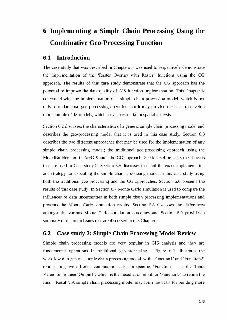
148
6 Implementing a Simple Chain Processing Using the
Combinative Geo-Processing Function
6.1 Introduction
The case study that was described in Chapters 5 was used to respectively demonstrate
the implementation of the ‘Raster Overlay with Raster’ functions using the CG
approach. The results of this case study demonstrate that the CG approach has the
potential to improve the data quality of GIS function implementation. This Chapter is
concerned with the implementation of a simple chain processing model, which is not
only a fundamental geo-processing operation, but it may provide the basis to develop
more complex GIS models, which are also essential in spatial analysis.
Section 6.2 discusses the characteristics of a generic simple chain processing model and
describes the geo-processing model that it is used in this case study. Section 6.3
describes the two different approaches that may be used for the implementation of any
simple chain processing model; the traditional geo-processing approach using the
ModelBuilder tool in ArcGIS and the CG approach. Section 6.4 presents the datasets
that are used in Case study 2. Section 6.5 discusses in detail the exact implementation
and strategy for executing the simple chain processing model in this case study using
both the traditional geo-processing and the CG approaches. Section 6.6 presents the
results of this case study. In Section 6.7 Monte Carlo simulation is used to compare the
influences of data uncertainties in both simple chain processing implementations and
presents the Monte Carlo simulation results. Section 6.8 discusses the differences
amongst the various Monte Carlo simulation outcomes and Section 6.9 provides a
summary of the main issues that are discussed in this Chapter.
6.2 Case study 2: Simple Chain Processing Model Review
Simple chain processing models are very popular in GIS analysis and they are
fundamental operations in traditional geo-processing. Figure 6-1 illustrates the
workflow of a generic simple chain processing model, with ‘Function1’ and ‘Function2’
representing two different computation tasks. In specific, ‘Function1’ uses the ‘Input
Value’ to produce ‘Output1’, which is then used as an input for ‘Function2’ to return the
final ‘Result’. A simple chain processing model may form the basis for building more
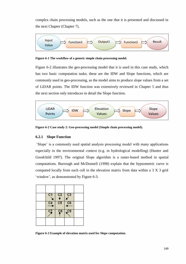
149
complex chain processing models, such as the one that it is presented and discussed in
the next Chapter (Chapter 7).
Figure 6-1 The workflow of a generic simple chain processing model.
Figure 6-2 illustrates the geo-processing model that it is used in this case study, which
has two basic computation tasks; these are the IDW and Slope functions, which are
commonly used in geo-processing, as the model aims to produce slope values from a set
of LiDAR points. The IDW function was extensively reviewed in Chapter 5 and thus
the next section only introduces in detail the Slope function.
Figure 6-2 Case study 2: Geo-processing model (Simple chain processing model).
6.2.1 Slope Function
‘Slope’ is a commonly used spatial analysis processing model with many applications
especially in the environmental context (e.g. in hydrological modelling) (Hunter and
Goodchild 1997). The original Slope algorithm is a raster-based method in spatial
computations. Burrough and McDonnell (1998) explain that the hypsometric curve is
computed locally from each cell in the elevation matrix from data within a 3 X 3 grid
‘window’, as demonstrated by Figure 6-3.
Figure 6-3 Example of elevation matrix used for Slope computation.
150
The geo-processing model of this case study uses the same Slope algorithm that it is
also used in ArcGIS. The same geo-processing model is used in order to later compare
the ArcGIS and the CG results and explore any data quality issues. The ArcGIS Slope
algorithm is a third-order finite difference estimate of the gradient in east-west and
south-north directions (Horn 1981). The computational equation is given by Formula
6.1.
Gradient (x) = [(C3 + 2C6 + C9) – (C1 + 2C4 + C7)] / (8 * бx)
Gradient (y) = [(C3 + 2C6 + C9) – (C1 + 2C4 + C7)] / (8 * бx) [6.1]
Slope is commonly measured in degrees based on the algorithm given by Formula 6.2
below.
Slope Degrees = ATAN (√ ([Gradient (x) ]^2 + [Gradient (y) ]^2) ) * 57.29578
[6.2]
The next section demonstrates the methodological approach for the implementation of
the simple chain processing model in both traditional geo-processing and the CG
approaches.
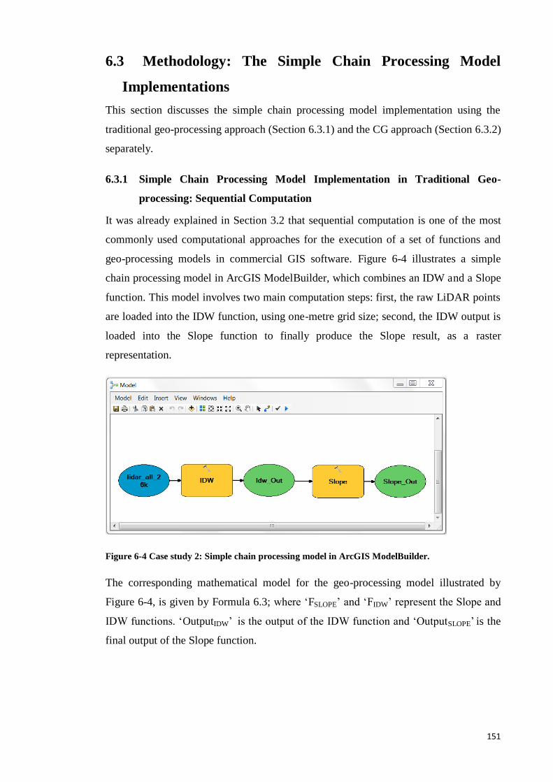
151
6.3 Methodology: The Simple Chain Processing Model
Implementations
This section discusses the simple chain processing model implementation using the
traditional geo-processing approach (Section 6.3.1) and the CG approach (Section 6.3.2)
separately.
6.3.1 Simple Chain Processing Model Implementation in Traditional Geo-
processing: Sequential Computation
It was already explained in Section 3.2 that sequential computation is one of the most
commonly used computational approaches for the execution of a set of functions and
geo-processing models in commercial GIS software. Figure 6-4 illustrates a simple
chain processing model in ArcGIS ModelBuilder, which combines an IDW and a Slope
function. This model involves two main computation steps: first, the raw LiDAR points
are loaded into the IDW function, using one-metre grid size; second, the IDW output is
loaded into the Slope function to finally produce the Slope result, as a raster
representation.
Figure 6-4 Case study 2: Simple chain processing model in ArcGIS ModelBuilder.
The corresponding mathematical model for the geo-processing model illustrated by
Figure 6-4, is given by Formula 6.3; where ‘FSLOPE’ and ‘FIDW’ represent the Slope and
IDW functions. ‘OutputIDW’ is the output of the IDW function and ‘OutputSLOPE’ is the
final output of the Slope function.
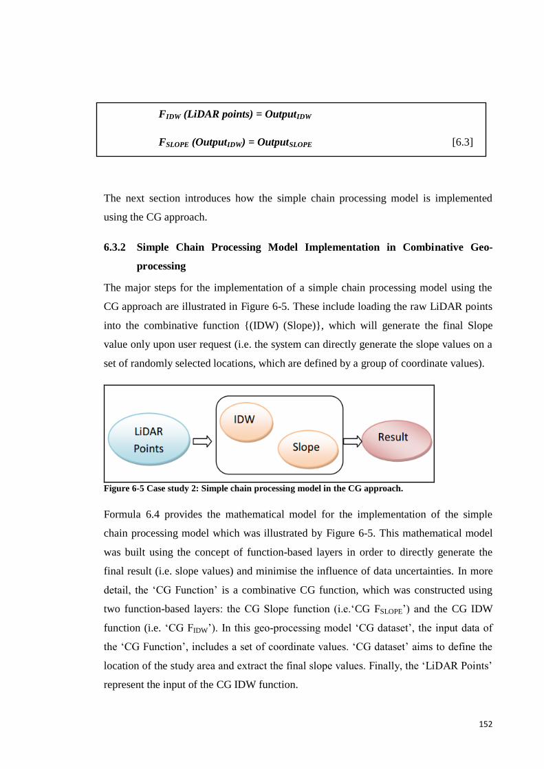
152
FIDW (LiDAR points) = OutputIDW
FSLOPE (OutputIDW) = OutputSLOPE [6.3]
The next section introduces how the simple chain processing model is implemented
using the CG approach.
6.3.2 Simple Chain Processing Model Implementation in Combinative Geo-
processing
The major steps for the implementation of a simple chain processing model using the
CG approach are illustrated in Figure 6-5. These include loading the raw LiDAR points
into the combinative function {(IDW) (Slope)}, which will generate the final Slope
value only upon user request (i.e. the system can directly generate the slope values on a
set of randomly selected locations, which are defined by a group of coordinate values).
Figure 6-5 Case study 2: Simple chain processing model in the CG approach.
Formula 6.4 provides the mathematical model for the implementation of the simple
chain processing model which was illustrated by Figure 6-5. This mathematical model
was built using the concept of function-based layers in order to directly generate the
final result (i.e. slope values) and minimise the influence of data uncertainties. In more
detail, the ‘CG Function’ is a combinative CG function, which was constructed using
two function-based layers: the CG Slope function (i.e.‘CG FSLOPE’) and the CG IDW
function (i.e. ‘CG FIDW’). In this geo-processing model ‘CG dataset’, the input data of
the ‘CG Function’, includes a set of coordinate values. ‘CG dataset’ aims to define the
location of the study area and extract the final slope values. Finally, the ‘LiDAR Points’
represent the input of the CG IDW function.
153
CG Function (CG dataset) =
{CG FSLOPE (CG FIDW (LiDAR Points)) (CG dataset)} [6.4]
Sections 6.3.1 and 6.3.2 discussed two different approaches that can be used for the
implementation and execution of a simple chain processing model. The fundamental
difference, is that in traditional geo-processing (i.e. ModelBuilder in ArcGIS) a
sequential computation approach is used to process the model and its tasks, while in the
CG approach a combinative function is used to directly execute it.
6.4 Case study 2: The Simple Chain Processing Model
Dataset
Figure 6-6 shows the sample of raw LiDAR point data used in this case study, as well
as, the geographical location (around 10,000 square metres) and the topographical
features within the study area (shown by the yellow rectangle in Bing Maps satellite
image in Figure 6-6). The sample dataset includes 26,499 points that were selected from
the original LiDAR dataset (i.e. the second group of the LiDAR dataset6). It should be
noted that in contrast to the first case study where 1,000 points were selected from the
original LiDAR dataset, this case study uses a significantly higher number of points in
order to further test the time performance of the CG approach in terms of processing
large spatial datasets.
6 Technical information of the second group of raw LiDAR dataset is provided in the Appendix A (Table
A.2).
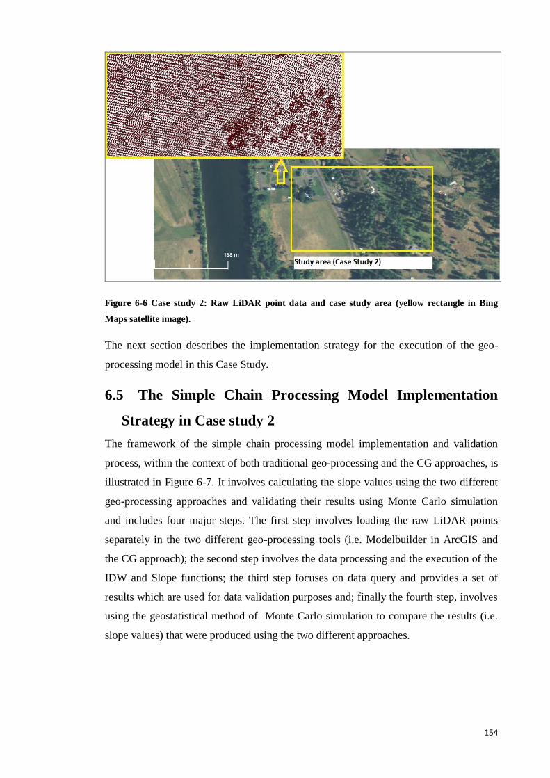
154
Figure 6-6 Case study 2: Raw LiDAR point data and case study area (yellow rectangle in Bing
Maps satellite image).
The next section describes the implementation strategy for the execution of the geo-
processing model in this Case Study.
6.5 The Simple Chain Processing Model Implementation
Strategy in Case study 2
The framework of the simple chain processing model implementation and validation
process, within the context of both traditional geo-processing and the CG approaches, is
illustrated in Figure 6-7. It involves calculating the slope values using the two different
geo-processing approaches and validating their results using Monte Carlo simulation
and includes four major steps. The first step involves loading the raw LiDAR points
separately in the two different geo-processing tools (i.e. Modelbuilder in ArcGIS and
the CG approach); the second step involves the data processing and the execution of the
IDW and Slope functions; the third step focuses on data query and provides a set of
results which are used for data validation purposes and; finally the fourth step, involves
using the geostatistical method of Monte Carlo simulation to compare the results (i.e.
slope values) that were produced using the two different approaches.
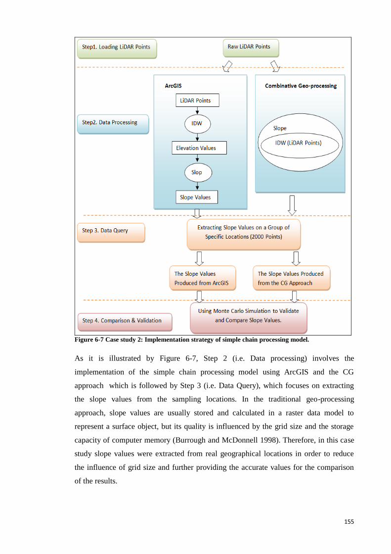
155
Figure 6-7 Case study 2: Implementation strategy of simple chain processing model.
As it is illustrated by Figure 6-7, Step 2 (i.e. Data processing) involves the
implementation of the simple chain processing model using ArcGIS and the CG
approach which is followed by Step 3 (i.e. Data Query), which focuses on extracting
the slope values from the sampling locations. In the traditional geo-processing
approach, slope values are usually stored and calculated in a raster data model to
represent a surface object, but its quality is influenced by the grid size and the storage
capacity of computer memory (Burrough and McDonnell 1998). Therefore, in this case
study slope values were extracted from real geographical locations in order to reduce
the influence of grid size and further providing the accurate values for the comparison
of the results.
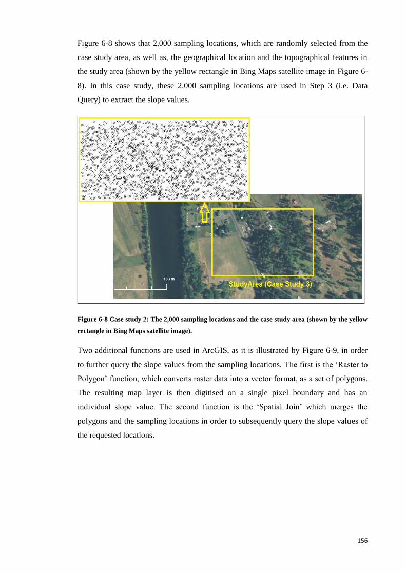
156
Figure 6-8 shows that 2,000 sampling locations, which are randomly selected from the
case study area, as well as, the geographical location and the topographical features in
the study area (shown by the yellow rectangle in Bing Maps satellite image in Figure 6-
8). In this case study, these 2,000 sampling locations are used in Step 3 (i.e. Data
Query) to extract the slope values.
Figure 6-8 Case study 2: The 2,000 sampling locations and the case study area (shown by the yellow
rectangle in Bing Maps satellite image).
Two additional functions are used in ArcGIS, as it is illustrated by Figure 6-9, in order
to further query the slope values from the sampling locations. The first is the ‘Raster to
Polygon’ function, which converts raster data into a vector format, as a set of polygons.
The resulting map layer is then digitised on a single pixel boundary and has an
individual slope value. The second function is the ‘Spatial Join’ which merges the
polygons and the sampling locations in order to subsequently query the slope values of
the requested locations.
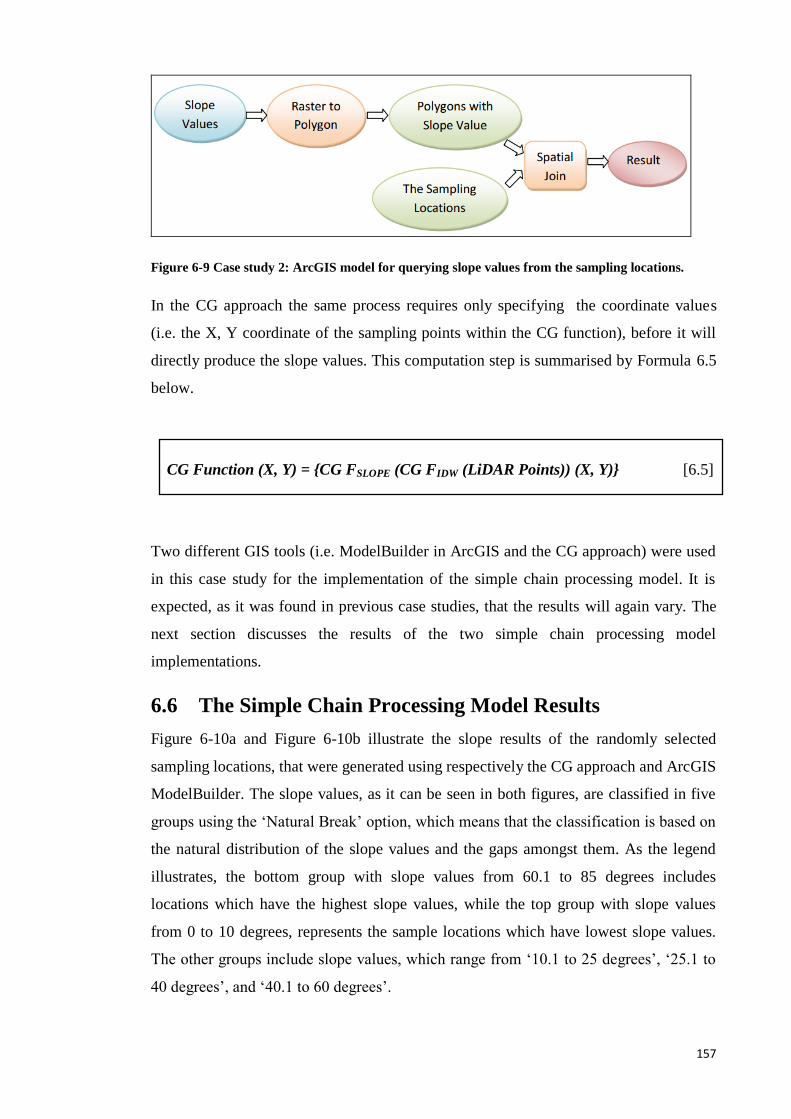
157
Figure 6-9 Case study 2: ArcGIS model for querying slope values from the sampling locations.
In the CG approach the same process requires only specifying the coordinate values
(i.e. the X, Y coordinate of the sampling points within the CG function), before it will
directly produce the slope values. This computation step is summarised by Formula 6.5
below.
CG Function (X, Y) = {CG FSLOPE (CG FIDW (LiDAR Points)) (X, Y)} [6.5]
Two different GIS tools (i.e. ModelBuilder in ArcGIS and the CG approach) were used
in this case study for the implementation of the simple chain processing model. It is
expected, as it was found in previous case studies, that the results will again vary. The
next section discusses the results of the two simple chain processing model
implementations.
6.6 The Simple Chain Processing Model Results
Figure 6-10a and Figure 6-10b illustrate the slope results of the randomly selected
sampling locations, that were generated using respectively the CG approach and ArcGIS
ModelBuilder. The slope values, as it can be seen in both figures, are classified in five
groups using the ‘Natural Break’ option, which means that the classification is based on
the natural distribution of the slope values and the gaps amongst them. As the legend
illustrates, the bottom group with slope values from 60.1 to 85 degrees includes
locations which have the highest slope values, while the top group with slope values
from 0 to 10 degrees, represents the sample locations which have lowest slope values.
The other groups include slope values, which range from ‘10.1 to 25 degrees’, ‘25.1 to
40 degrees’, and ‘40.1 to 60 degrees’.
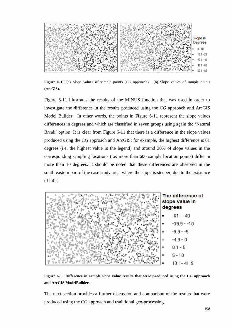
158
Figure 6-10 (a) Slope values of sample points (CG approach). (b) Slope values of sample points
(ArcGIS).
Figure 6-11 illustrates the results of the MINUS function that was used in order to
investigate the difference in the results produced using the CG approach and ArcGIS
Model Builder. In other words, the points in Figure 6-11 represent the slope values
differences in degrees and which are classified in seven groups using again the ‘Natural
Break’ option. It is clear from Figure 6-11 that there is a difference in the slope values
produced using the CG approach and ArcGIS; for example, the highest difference is 61
degrees (i.e. the highest value in the legend) and around 30% of slope values in the
corresponding sampling locations (i.e. more than 600 sample location points) differ in
more than 10 degrees. It should be noted that these differences are observed in the
south-eastern part of the case study area, where the slope is steeper, due to the existence
of hills.
Figure 6-11 Difference in sample slope value results that were produced using the CG approach
and ArcGIS ModelBuilder.
The next section provides a further discussion and comparison of the results that were
produced using the CG approach and traditional geo-processing.
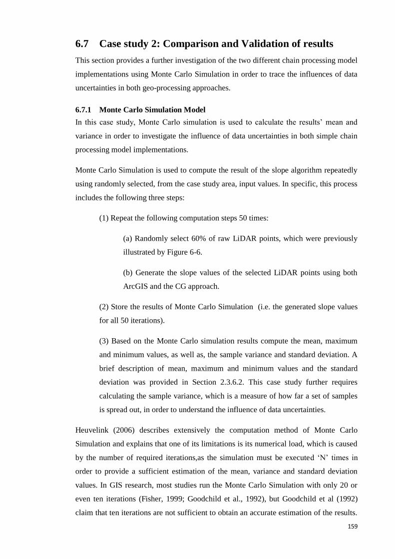
159
6.7 Case study 2: Comparison and Validation of results
This section provides a further investigation of the two different chain processing model
implementations using Monte Carlo Simulation in order to trace the influences of data
uncertainties in both geo-processing approaches.
6.7.1 Monte Carlo Simulation Model
In this case study, Monte Carlo simulation is used to calculate the results’ mean and
variance in order to investigate the influence of data uncertainties in both simple chain
processing model implementations.
Monte Carlo Simulation is used to compute the result of the slope algorithm repeatedly
using randomly selected, from the case study area, input values. In specific, this process
includes the following three steps:
(1) Repeat the following computation steps 50 times:
(a) Randomly select 60% of raw LiDAR points, which were previously
illustrated by Figure 6-6.
(b) Generate the slope values of the selected LiDAR points using both
ArcGIS and the CG approach.
(2) Store the results of Monte Carlo Simulation (i.e. the generated slope values
for all 50 iterations).
(3) Based on the Monte Carlo simulation results compute the mean, maximum
and minimum values, as well as, the sample variance and standard deviation. A
brief description of mean, maximum and minimum values and the standard
deviation was provided in Section 2.3.6.2. This case study further requires
calculating the sample variance, which is a measure of how far a set of samples
is spread out, in order to understand the influence of data uncertainties.
Heuvelink (2006) describes extensively the computation method of Monte Carlo
Simulation and explains that one of its limitations is its numerical load, which is caused
by the number of required iterations,as the simulation must be executed ‘N’ times in
order to provide a sufficient estimation of the mean, variance and standard deviation
values. In GIS research, most studies run the Monte Carlo Simulation with only 20 or
even ten iterations (Fisher, 1999; Goodchild et al., 1992), but Goodchild et al (1992)
claim that ten iterations are not sufficient to obtain an accurate estimation of the results.
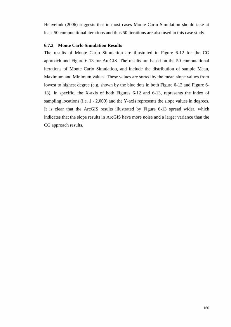
160
Heuvelink (2006) suggests that in most cases Monte Carlo Simulation should take at
least 50 computational iterations and thus 50 iterations are also used in this case study.
6.7.2 Monte Carlo Simulation Results
The results of Monte Carlo Simulation are illustrated in Figure 6-12 for the CG
approach and Figure 6-13 for ArcGIS. The results are based on the 50 computational
iterations of Monte Carlo Simulation, and include the distribution of sample Mean,
Maximum and Minimum values. These values are sorted by the mean slope values from
lowest to highest degree (e.g. shown by the blue dots in both Figure 6-12 and Figure 6-
13). In specific, the X-axis of both Figures 6-12 and 6-13, represents the index of
sampling locations (i.e. 1 - 2,000) and the Y-axis represents the slope values in degrees.
It is clear that the ArcGIS results illustrated by Figure 6-13 spread wider, which
indicates that the slope results in ArcGIS have more noise and a larger variance than the
CG approach results.
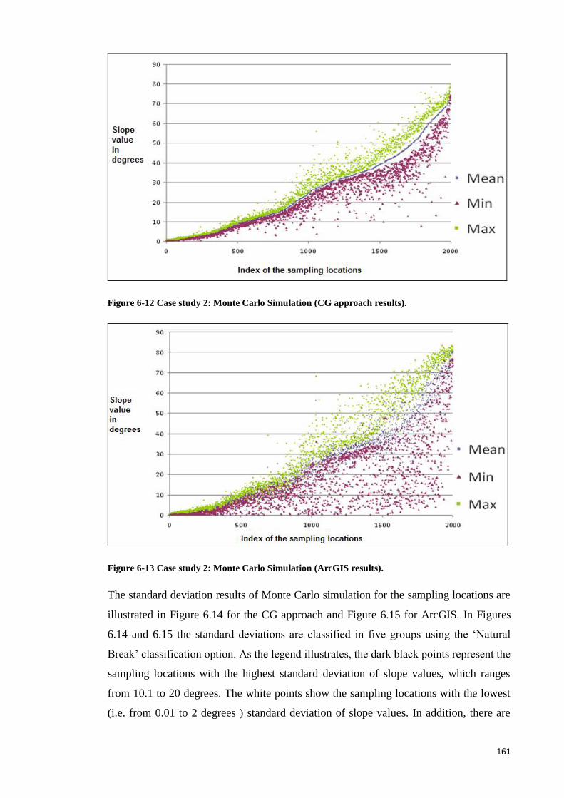
161
Figure 6-12 Case study 2: Monte Carlo Simulation (CG approach results).
Figure 6-13 Case study 2: Monte Carlo Simulation (ArcGIS results).
The standard deviation results of Monte Carlo simulation for the sampling locations are
illustrated in Figure 6.14 for the CG approach and Figure 6.15 for ArcGIS. In Figures
6.14 and 6.15 the standard deviations are classified in five groups using the ‘Natural
Break’ classification option. As the legend illustrates, the dark black points represent the
sampling locations with the highest standard deviation of slope values, which ranges
from 10.1 to 20 degrees. The white points show the sampling locations with the lowest
(i.e. from 0.01 to 2 degrees ) standard deviation of slope values. In addition, there are
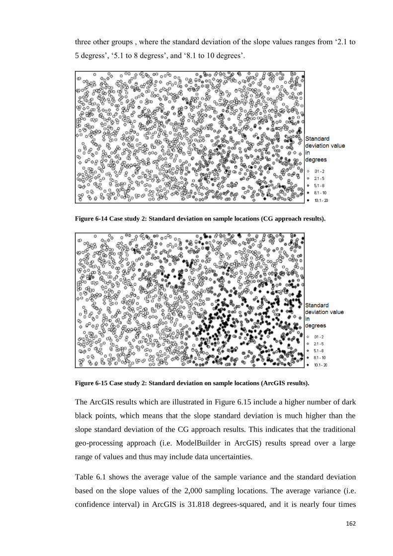
162
three other groups , where the standard deviation of the slope values ranges from ‘2.1 to
5 degress’, ‘5.1 to 8 degress’, and ‘8.1 to 10 degrees’.
Figure 6-14 Case study 2: Standard deviation on sample locations (CG approach results).
Figure 6-15 Case study 2: Standard deviation on sample locations (ArcGIS results).
The ArcGIS results which are illustrated in Figure 6.15 include a higher number of dark
black points, which means that the slope standard deviation is much higher than the
slope standard deviation of the CG approach results. This indicates that the traditional
geo-processing approach (i.e. ModelBuilder in ArcGIS) results spread over a large
range of values and thus may include data uncertainties.
Table 6.1 shows the average value of the sample variance and the standard deviation
based on the slope values of the 2,000 sampling locations. The average variance (i.e.
confidence interval) in ArcGIS is 31.818 degrees-squared, and it is nearly four times

163
larger than CG approach’s average variance, which is 7.304 degrees-squared. Also the
average standard deviation in ArcGIS, which is equal to 3.844 degrees, is nearly two
times larger than CG approach’s standard deviation, which is equal to 1.811 degrees.
Table 6-1 further indicates that the ArcGIS results have a larger distribution than the CG
approach results, which means that they include data uncertainties.
Table 6-1 Case study 2: A comparison of variance and standard deviation.
ArcGIS Results (Average
value)
CG Results
Average of Variance 31.818 degrees-squared 7.304 degrees-squared
Average of Standard
Deviation
3.844 degrees 1.811 degrees
6.8 Discussion
Monte Carlo simulation analysis revealed many differences between the CG and
traditional geo-processing results. These may occur due to mainly two reasons, which
are discussed in the following paragraphs.
First, the two approaches differ in terms of storing numerical numbers. In traditional
geo-processing, numerical computation is a common method to store the results.
However, one problem with numerical computation is round-off values, which may
result in round-off errors (Goldberg 1994). Table 6-2 provides some examples of round-
off errors that may occur in numerical computation. For example, if ‘log10 2’ is rounded
to three decimal places (i.e. 0.301), the total round-off error is
‘0.000 029 995 663 981 195 21’. It should be noted that increasing the number of
decimal digits may reduce the magnitude of round-off error, but limited computer
storage memory may still cause round-off errors in various real numbers. On the other
hand, the CG approach uses symbolic computation, which improves the precision of
various calculations. Moreover, in the CG approach round-off errors do not exist
because symbols and algebraic relationships are manipulated without storing numerical
values (Recktenwald 2006).

164
Table 6-2 Example of round-off errors in numerical computation.
Real
Number
Representation
Value
Approximation
Value
Round-off Error
1/7 0.142 857 0.142 857 0.000 000 142 857
ln 2 0.693 147 180 559 945 309 41... 0.693 147 0.000 000 180 559 945 309 41...
log10 2 0.301 029 995 663 981 195 21... 0.301 0.000 029 995 663 981 195 21...
∛ 2 1.259 921 049 894 873 164 76... 1.25992 0.000 001 049 894 873 164 76...
√ 2 1.414 213 562 373 095 048 80... 1.41421 0.000 003 562 373 095 048 80...
Second, spatial attributes, such as elevation and slope, are represented as raster layers in
the traditional geo-processing approach, which have an arbitrary resolution and may
cause data uncertainties (Haklay 2004). For instance, Figure 6-16 shows how slope can
be represented in a raster-based layer, where each grid is assigned with a value that
records the slope value from the centre of the grid (shown by the red cross in Figure 6-
16). In the traditional geo-processing approach, all geographical points, that belong to
the grid are assigned with the same slope value, which is assigned to the centre of the
grid. As a result, the distance shift (shown by the black arrow in Figure 6-16) between
the randomly selected locations and the centre of the grid may cause distortions in the
slope values. These data uncertainties may be propagated when the slope values are
used as an input into further computation tasks in a traditional geo-processing model.
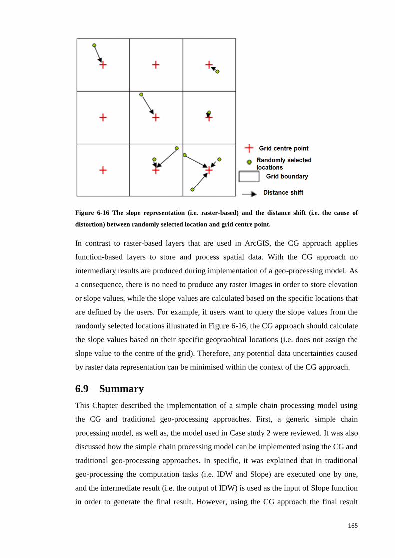
165
Figure 6-16 The slope representation (i.e. raster-based) and the distance shift (i.e. the cause of
distortion) between randomly selected location and grid centre point.
In contrast to raster-based layers that are used in ArcGIS, the CG approach applies
function-based layers to store and process spatial data. With the CG approach no
intermediary results are produced during implementation of a geo-processing model. As
a consequence, there is no need to produce any raster images in order to store elevation
or slope values, while the slope values are calculated based on the specific locations that
are defined by the users. For example, if users want to query the slope values from the
randomly selected locations illustrated in Figure 6-16, the CG approach should calculate
the slope values based on their specific geopraohical locations (i.e. does not assign the
slope value to the centre of the grid). Therefore, any potential data uncertainties caused
by raster data representation can be minimised within the context of the CG approach.
6.9 Summary
This Chapter described the implementation of a simple chain processing model using
the CG and traditional geo-processing approaches. First, a generic simple chain
processing model, as well as, the model used in Case study 2 were reviewed. It was also
discussed how the simple chain processing model can be implemented using the CG and
traditional geo-processing approaches. In specific, it was explained that in traditional
geo-processing the computation tasks (i.e. IDW and Slope) are executed one by one,
and the intermediate result (i.e. the output of IDW) is used as the input of Slope function
in order to generate the final result. However, using the CG approach the final result
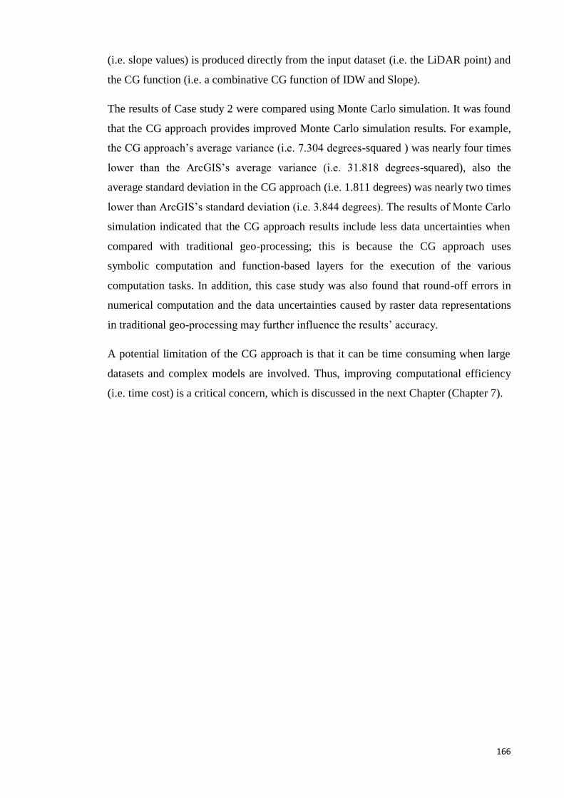
166
(i.e. slope values) is produced directly from the input dataset (i.e. the LiDAR point) and
the CG function (i.e. a combinative CG function of IDW and Slope).
The results of Case study 2 were compared using Monte Carlo simulation. It was found
that the CG approach provides improved Monte Carlo simulation results. For example,
the CG approach’s average variance (i.e. 7.304 degrees-squared ) was nearly four times
lower than the ArcGIS’s average variance (i.e. 31.818 degrees-squared), also the
average standard deviation in the CG approach (i.e. 1.811 degrees) was nearly two times
lower than ArcGIS’s standard deviation (i.e. 3.844 degrees). The results of Monte Carlo
simulation indicated that the CG approach results include less data uncertainties when
compared with traditional geo-processing; this is because the CG approach uses
symbolic computation and function-based layers for the execution of the various
computation tasks. In addition, this case study was also found that round-off errors in
numerical computation and the data uncertainties caused by raster data representations
in traditional geo-processing may further influence the results’ accuracy.
A potential limitation of the CG approach is that it can be time consuming when large
datasets and complex models are involved. Thus, improving computational efficiency
(i.e. time cost) is a critical concern, which is discussed in the next Chapter (Chapter 7).
167
7 Implementing a Complex Chain Processing Model
Using Combinative Geo-processing Function
7.1 Introduction
The previous Chapter (Chapter 7) demonstrated how a simple chain processing model is
implemented in the CG approach. The Monte Carlo simulation results of Case Study 2
show that the CG approach helps to overcome and improve data uncertainty problems
which exist in the traditional geo-processing. Nevertheless, it is should be noted that the
simple chain processing model implementation using the CG approach increases the
required computation time, possibly due to the inefficient computation strategy used in
the execution and manipulation of geographical data and GIS functions. To further
investigate and resolve this implication this case study focuses on the efficiency (i.e.
computation time) of the computation strategy of the CG approach.
Section 7.2 discusses the implications of inefficient computation strategy in geo-
processing and introduces the concepts of computation flexibility and computation
sequence. Section 7.3 proposes the concept of CG computation priority, which aims to
reduce the overall computation time of geo-processing through the use of an improved
computation strategy. Section 7.4 reviews the complex chain processing model that it is
applied in this case study and Section 7.5 discusses how the model is implemented in
traditional geo-processing and the CG approach using computation priority. Section 7.6
presents the datasets that are used in Case study 3. Section 7.7 discusses in detail the
exact implementation and strategy for executing the complex chain processing model in
this case study using the two different geo-processing approaches. Section 7.8 presents
the results of the complex chain processing model implementations. Section 7.9
compares the implementation results of the overall computation time and Section 7.10
discusses the significant differences of the results. Finally, Section 7.11 provides a
summary of the main issues that are discussed in this Chapter.
7.2 The Implications of Computation Strategy in Geo-
processing
The first two case studies described in Chapters 5 and 6, mainly focused on the
improvement of data uncertainty using the CG approach. Nevertheless, it became
evident that a problem of the previous CG implementations was concerned with the
168
required computation time. Specifically, intensive computation time is usually required
to implement the various CG functions and the computations based on Higher-Order
Functions in order to reduce the influence of data uncertainties in the geo-processing. In
some case studies, especially those which involve large spatial datasets (e.g. in Case
Study 3), the computation time of processing the LiDAR point dataset (around 26,000
points) and the CG functions (‘IDW’ and ‘Slope’) required several hours in the current
CG approach (i.e. without an efficient computationa strategy). To further investigate
and address this problem, Case study 3 focuses on computational efficiency and it
involves the implementation of a complex geo-processing model with larger spatial
datasets.
This section discusses the implications of computation strategy as it is a fundamental
element for improving computational efficiency (Loogen et al., 1993; Fijany et al.,
1995). Computation strategy represents a plan, which is used to solve one or more goals
by applying an optimum method in order to efficiently control the computations (Martin
and Virseda 2005). For example, Loogen et al., (1993) discuss a computation strategy
for lazy conditional narrowing, which is based on the idea of transforming patterns into
decision trees to manage the computation; Manoranjan et al., (2004) also describe new
efficient similarity metric and generic computation strategy for pattern-based very low
bit-rate video coding. These examples show that an optimum computation strategy may
potentially improve computational efficiency.
In this thesis, the computation strategy of the traditional geo-processing approach has
been discussed in Case Studies 1 and 2, which showed that the computation tasks (i.e.
GIS functions) of a geo-processing model are executed sequentially in the traditional
geo-processing approach. Moreover, it was also found from these case studies that there
are two factors which frequently influence the existing computation strategy and which
may extend the overall computation time, and these refer to computation flexibility and
computation sequence. Computation flexibility refers to the procedures that can manage
the allocations of costly resources, such as time, memory, or information (Martin and
Virseda 2005). Computation sequence represents the execution order of computation
tasks in a geo-processing model.
Computation flexibility may influence the efficiency of a computation strategy
implementation because an optimum computation strategy needs a capability to control
the computations and manage the costs, such as amount of computation resources and
calculations (Martin and Virseda 2005). The earlier case studies showed that the current
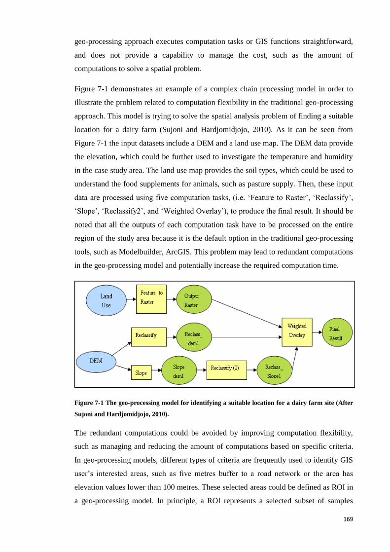
169
geo-processing approach executes computation tasks or GIS functions straightforward,
and does not provide a capability to manage the cost, such as the amount of
computations to solve a spatial problem.
Figure 7-1 demonstrates an example of a complex chain processing model in order to
illustrate the problem related to computation flexibility in the traditional geo-processing
approach. This model is trying to solve the spatial analysis problem of finding a suitable
location for a dairy farm (Sujoni and Hardjomidjojo, 2010). As it can be seen from
Figure 7-1 the input datasets include a DEM and a land use map. The DEM data provide
the elevation, which could be further used to investigate the temperature and humidity
in the case study area. The land use map provides the soil types, which could be used to
understand the food supplements for animals, such as pasture supply. Then, these input
data are processed using five computation tasks, (i.e. ‘Feature to Raster’, ‘Reclassify’,
‘Slope’, ‘Reclassify2’, and ‘Weighted Overlay’), to produce the final result. It should be
noted that all the outputs of each computation task have to be processed on the entire
region of the study area because it is the default option in the traditional geo-processing
tools, such as Modelbuilder, ArcGIS. This problem may lead to redundant computations
in the geo-processing model and potentially increase the required computation time.
Figure 7-1 The geo-processing model for identifying a suitable location for a dairy farm site (After
Sujoni and Hardjomidjojo, 2010).
The redundant computations could be avoided by improving computation flexibility,
such as managing and reducing the amount of computations based on specific criteria.
In geo-processing models, different types of criteria are frequently used to identify GIS
user’s interested areas, such as five metres buffer to a road network or the area has
elevation values lower than 100 metres. These selected areas could be defined as ROI in
a geo-processing model. In principle, a ROI represents a selected subset of samples

170
within a dataset identified for a particular purpose, and possibly covers only a part of the
entire study area.
For instance, in the geo-processing model displayed in Figure 7-1, one of the site
selection criteria is that the proposed for the dairy farm site should be located within a
pasture area. This means that any data located outside the pasture area will not be
considered in the GIS analysis, so no further processing of these data is required. As
Figure 7-2 shows the ROI of this geo-processing model, which includes the pasture
area, takes approximately 20% of the entire region, which means that the outside of the
ROI area data, (almost the 80% of the entire region), will not require any further
processing. Therefore if further processing of data outside of the ROI area can be
avoided, it could significantly improve computational efficiency.
Figure 7-2 Region Of Interest (ROI), which shows the pasture area of the dairy farm model.
Moreover, computation sequence, which provides an order to execute various
computation tasks in a geo-processing model, may also influence the efficiency of the
computation strategy. As was discussed in Chapter 3 that current geo-processing tools
use a sequential computation sequence to execute the computation tasks that are
included in a geo-processing model. This is mainly because popular geo-processing
tools (e.g. ArcGIS and MapInfo) are developed using programming languages such as
JAVA and C, where the so-called ‘Call-by-Value’ computation strategy is used to store
and calculate a value. The major characteristic of the ‘Call-by-Value’ computation
strategy is that the argument of a function (e.g. x is a single argument in the function:
171
f(x) = x2 + 2) is calculated before the argument is used and the resulting values are
bound to the corresponding variables in the function (Lengrand 2003).
For instance, the implementation of a single GIS function in ArcGIS, which is
developed in C programming language, includes: (a) the ‘input’, which is an argument;
(b) when the ‘input’ loads into a GIS function, the resulting value is executed and
bounded to the corresponding variable (i.e. output). This computation strategy is
repeatedly applied in a chain sequence in order to implement all computation tasks of a
geo-processing model. Nevertheless, this chain computation sequence may not be
efficient when large geo-processing models are involved; it may include computations
that are not necessary to be executed at run time (Muchnick 1997, p.117).
Due to the previously noted computation strategy implications, the next section
introduces the concept of CG computation priority, which aims at improving the overall
computation time of a geo-processing model.
7.3 Implementations Combinative Geo-processing
Computation Priority
CG computation priority is an important computation rule in this research. It is used in
the CG approach and enables the execution of computation tasks or functions that are
included in a geo-processing model using a different computation strategy. Specifically,
the computation tasks are assigned initially with different priority values, and then they
are implemented according to this priority value, from highest to lowest.
7.3.1 Improving GIS Computational efficiency
Nowadays, GIS have been widely used in various fields, such as transportation,
environmental modelling, asset management, and citizen science. Nevertheless,
computational efficiency is a major concern of GIS development as the size of spatial
datasets and the complexity of spatial problems are dramatically increasing (Brown and
Coenen 2000).
There are many methods that can be used to improve computational efficiency and
performance of existing GIS technologies, such as spatial data structure and data access
methods which provide a way to access and query larger spatial databases more
efficiently. For example, Guttman (1984) states a spatial data access method, the so-
called R tree, to store, search, and query spatial information. R-tree provides an efficient
way to query a spatial database as computer memory and temporary database usage are
172
reduced in this method. R-tree has been widely used in different applications of spatial
data management. For example, R-trees are commonly used to store spatial data such
road networks and city locations, and then for querying the data quickly and efficiently
such as ‘Find a shortest distance from city A to city B’ or ‘Find a nearest motorway
access point around city C’. Moreover, Kriegel et al., (1993) discuss a method which
combines spatial access and computational geometry concepts in order to improve the
performance of GIS operations. The method could be applied in different applications
or algorithms, such as map overlay and map merge. However, the current method relies
on certain criteria (e.g. the robust spatial access method) and the further investigation is
needed to design efficient algorithms based on spatial access methods and
computational geometry for all retrieval operations.
The previously noted methodologies contribute to the GIS computations, especially
with respect to accessing and querying large spatial datasets. Nevertheless, these
methods do not improve the efficiency of executing a large group of computation tasks
in a geo-processing model.
7.3.2 Computation Combinative Geo-processing (CG) Computation Priority
Computation priority, or scheduling, is a common method used to effectively use
computation resources and improve computation performance (Jones et al., 1997). In
computer science, the priority (or scheduling) is used for implementing multiple
computation tasks. For example, the scheduling could be used to suspend a computation
task which has a low priority, or a computation task which is allocating a large amount
of memory in order to free up main memory for other computation tasks, implementing
the computation task later when more computer memory is available (Stallings 2004).
Moreover, the priority (or scheduling) has also been widely applied in GIS, mainly for
the purposes of determining least cost paths across a continuous surface (De Smith et
al., 2007).
Similarly to the priority rule that it is used in computer science or in spatial problems of
path selection, the CG computation priority is trying to provide a new computation
strategy in geo-processing to implement various computation tasks more efficiently, or
in other words, using the minimum computation time and computer resources.
Specifically, the basic principle of CG computation priority is that the CG approach
starts with an analysis of the computation tasks or GIS functions included in the geo-
processing model and then the system assigns priority values to each computation task
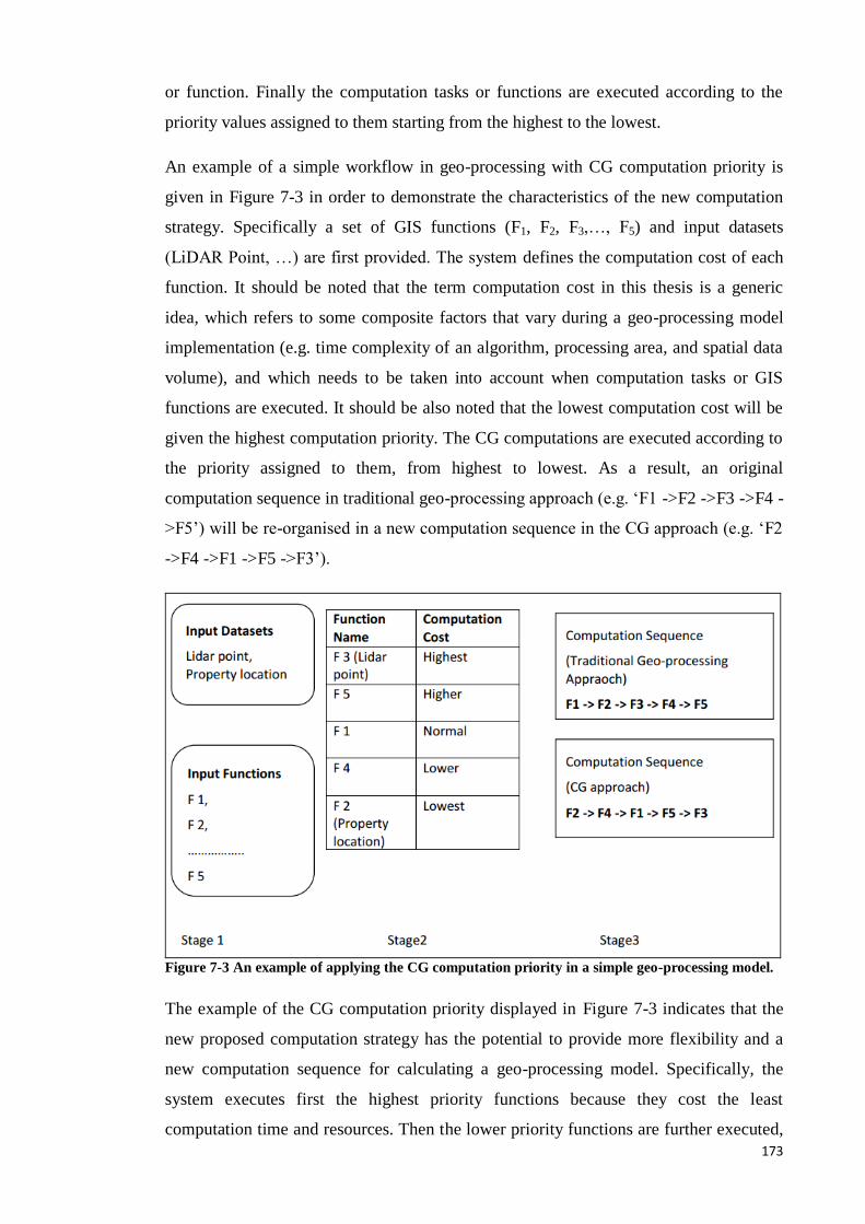
173
or function. Finally the computation tasks or functions are executed according to the
priority values assigned to them starting from the highest to the lowest.
An example of a simple workflow in geo-processing with CG computation priority is
given in Figure 7-3 in order to demonstrate the characteristics of the new computation
strategy. Specifically a set of GIS functions (F1, F2, F3,…, F5) and input datasets
(LiDAR Point, …) are first provided. The system defines the computation cost of each
function. It should be noted that the term computation cost in this thesis is a generic
idea, which refers to some composite factors that vary during a geo-processing model
implementation (e.g. time complexity of an algorithm, processing area, and spatial data
volume), and which needs to be taken into account when computation tasks or GIS
functions are executed. It should be also noted that the lowest computation cost will be
given the highest computation priority. The CG computations are executed according to
the priority assigned to them, from highest to lowest. As a result, an original
computation sequence in traditional geo-processing approach (e.g. ‘F1 ->F2 ->F3 ->F4 -
>F5’) will be re-organised in a new computation sequence in the CG approach (e.g. ‘F2
->F4 ->F1 ->F5 ->F3’).
Figure 7-3 An example of applying the CG computation priority in a simple geo-processing model.
The example of the CG computation priority displayed in Figure 7-3 indicates that the
new proposed computation strategy has the potential to provide more flexibility and a
new computation sequence for calculating a geo-processing model. Specifically, the
system executes first the highest priority functions because they cost the least
computation time and resources. Then the lower priority functions are further executed,
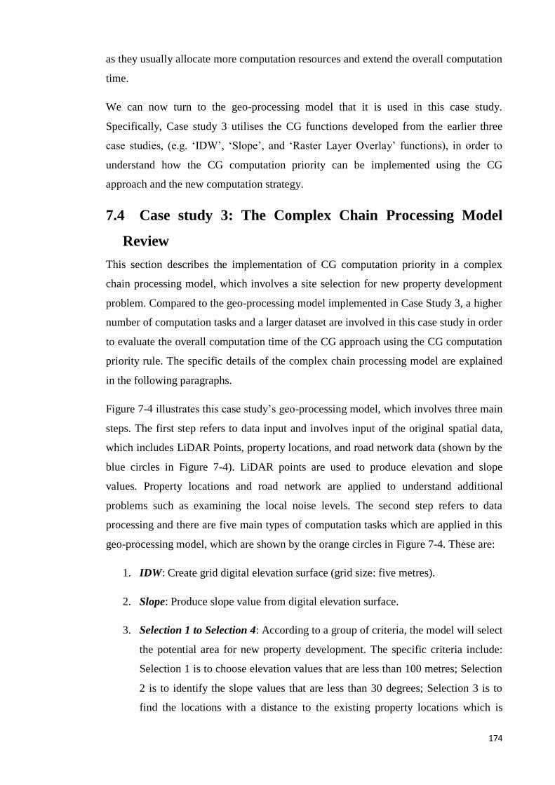
174
as they usually allocate more computation resources and extend the overall computation
time.
We can now turn to the geo-processing model that it is used in this case study.
Specifically, Case study 3 utilises the CG functions developed from the earlier three
case studies, (e.g. ‘IDW’, ‘Slope’, and ‘Raster Layer Overlay’ functions), in order to
understand how the CG computation priority can be implemented using the CG
approach and the new computation strategy.
7.4 Case study 3: The Complex Chain Processing Model
Review
This section describes the implementation of CG computation priority in a complex
chain processing model, which involves a site selection for new property development
problem. Compared to the geo-processing model implemented in Case Study 3, a higher
number of computation tasks and a larger dataset are involved in this case study in order
to evaluate the overall computation time of the CG approach using the CG computation
priority rule. The specific details of the complex chain processing model are explained
in the following paragraphs.
Figure 7-4 illustrates this case study’s geo-processing model, which involves three main
steps. The first step refers to data input and involves input of the original spatial data,
which includes LiDAR Points, property locations, and road network data (shown by the
blue circles in Figure 7-4). LiDAR points are used to produce elevation and slope
values. Property locations and road network are applied to understand additional
problems such as examining the local noise levels. The second step refers to data
processing and there are five main types of computation tasks which are applied in this
geo-processing model, which are shown by the orange circles in Figure 7-4. These are:
1. IDW: Create grid digital elevation surface (grid size: five metres).
2. Slope: Produce slope value from digital elevation surface.
3. Selection 1 to Selection 4: According to a group of criteria, the model will select
the potential area for new property development. The specific criteria include:
Selection 1 is to choose elevation values that are less than 100 metres; Selection
2 is to identify the slope values that are less than 30 degrees; Selection 3 is to
find the locations with a distance to the existing property locations which is
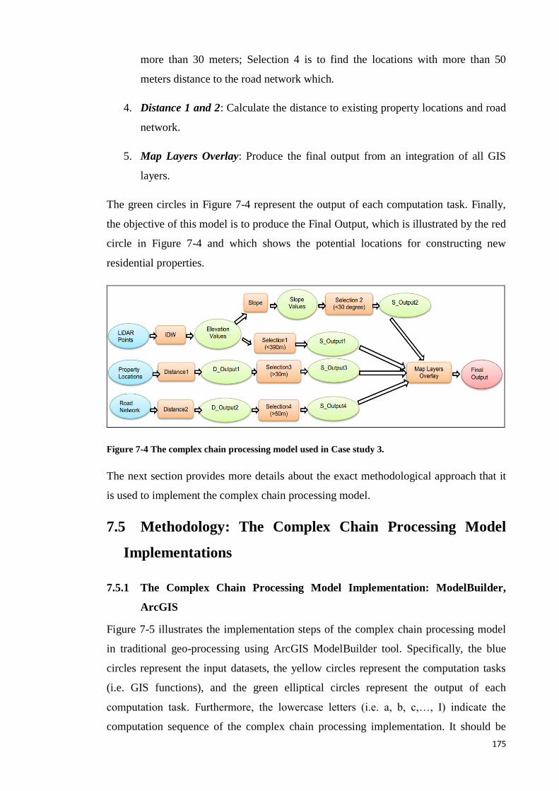
175
more than 30 meters; Selection 4 is to find the locations with more than 50
meters distance to the road network which.
4. Distance 1 and 2: Calculate the distance to existing property locations and road
network.
5. Map Layers Overlay: Produce the final output from an integration of all GIS
layers.
The green circles in Figure 7-4 represent the output of each computation task. Finally,
the objective of this model is to produce the Final Output, which is illustrated by the red
circle in Figure 7-4 and which shows the potential locations for constructing new
residential properties.
Figure 7-4 The complex chain processing model used in Case study 3.
The next section provides more details about the exact methodological approach that it
is used to implement the complex chain processing model.
7.5 Methodology: The Complex Chain Processing Model
Implementations
7.5.1 The Complex Chain Processing Model Implementation: ModelBuilder,
ArcGIS
Figure 7-5 illustrates the implementation steps of the complex chain processing model
in traditional geo-processing using ArcGIS ModelBuilder tool. Specifically, the blue
circles represent the input datasets, the yellow circles represent the computation tasks
(i.e. GIS functions), and the green elliptical circles represent the output of each
computation task. Furthermore, the lowercase letters (i.e. a, b, c,…, I) indicate the
computation sequence of the complex chain processing implementation. It should be
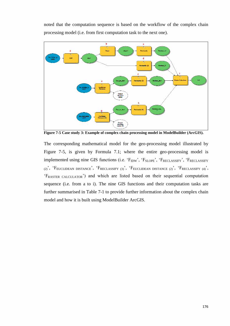
176
noted that the computation sequence is based on the workflow of the complex chain
processing model (i.e. from first computation task to the next one).
Figure 7-5 Case study 3: Example of complex chain processing model in ModelBuilder (ArcGIS).
The corresponding mathematical model for the geo-processing model illustrated by
Figure 7-5, is given by Formula 7.1; where the entire geo-processing model is
implemented using nine GIS functions (i.e. ‘FIDW’, ‘FSLOPE’, ‘FRECLASSIFY’, ‘FRECLASSIFY
(2)’, ‘FEUCLIDEAN DISTANCE’, ‘FRECLASSIFY (3)’, ‘FEUCLIDEAN DISTANCE (2)’, ‘FRECLASSIFY (4)’,
‘FRASTER CALCULATOR’) and which are listed based on their sequential computation
sequence (i.e. from a to i). The nine GIS functions and their computation tasks are
further summarised in Table 7-1 to provide further information about the complex chain
model and how it is built using ModelBuilder ArcGIS.
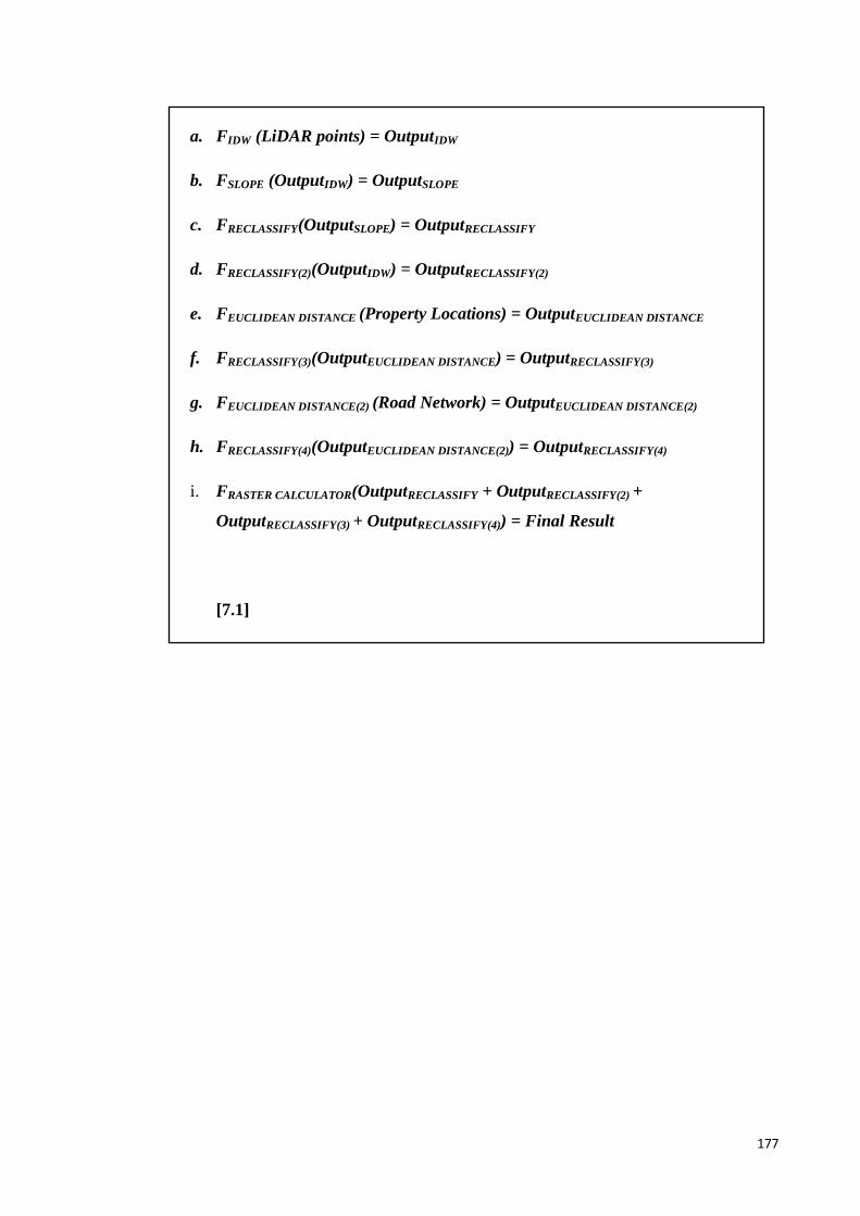
177
a. FIDW (LiDAR points) = OutputIDW
b. FSLOPE (OutputIDW) = OutputSLOPE
c. FRECLASSIFY(OutputSLOPE) = OutputRECLASSIFY
d. FRECLASSIFY(2)(OutputIDW) = OutputRECLASSIFY(2)
e. FEUCLIDEAN DISTANCE (Property Locations) = OutputEUCLIDEAN DISTANCE
f. FRECLASSIFY(3)(OutputEUCLIDEAN DISTANCE) = OutputRECLASSIFY(3)
g. FEUCLIDEAN DISTANCE(2) (Road Network) = OutputEUCLIDEAN DISTANCE(2)
h. FRECLASSIFY(4)(OutputEUCLIDEAN DISTANCE(2)) = OutputRECLASSIFY(4)
i. FRASTER CALCULATOR(OutputRECLASSIFY + OutputRECLASSIFY(2) +
OutputRECLASSIFY(3) + OutputRECLASSIFY(4)) = Final Result
[7.1]
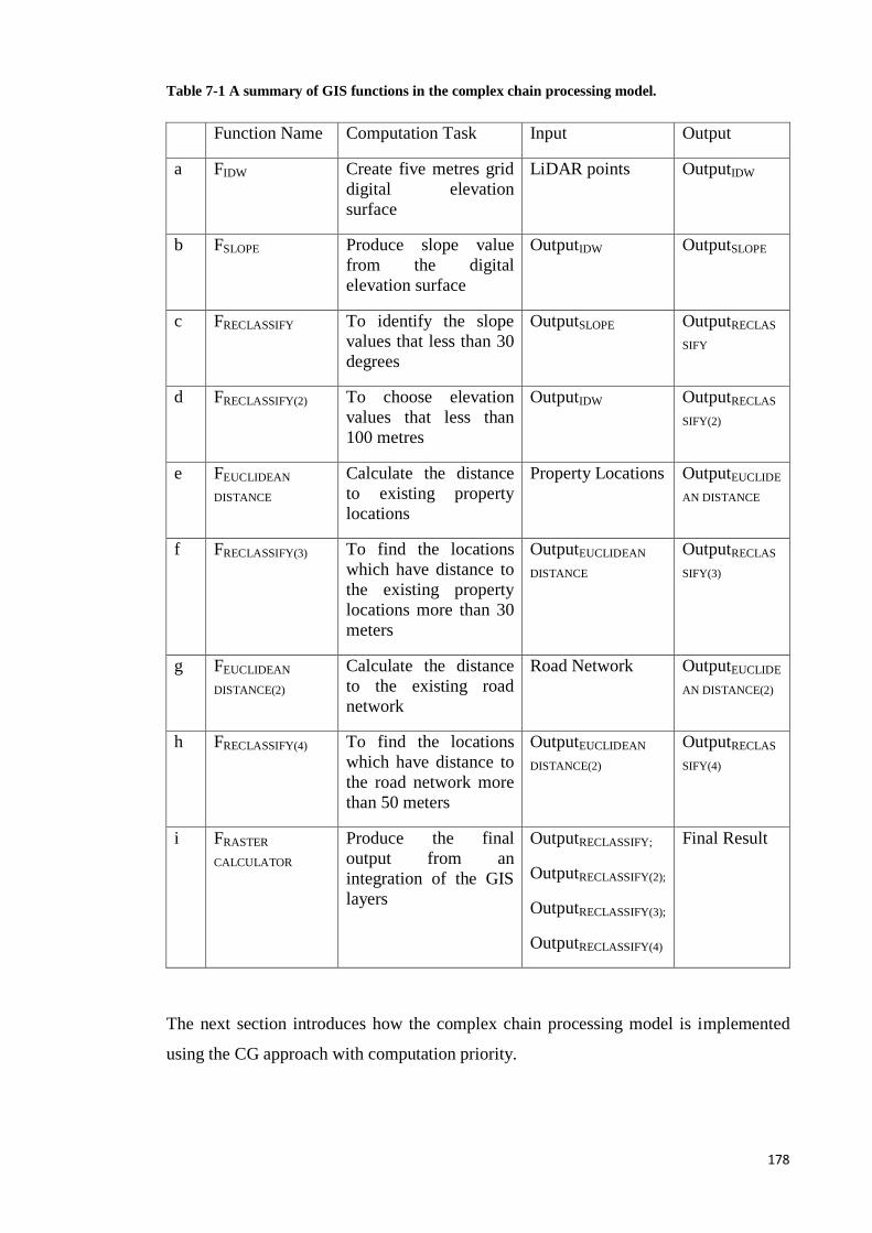
178
Table 7-1 A summary of GIS functions in the complex chain processing model.
Function Name Computation Task Input Output
a FIDW Create five metres grid
digital elevation
surface
LiDAR points OutputIDW
b FSLOPE Produce slope value
from the digital
elevation surface
OutputIDW OutputSLOPE
c FRECLASSIFY To identify the slope
values that less than 30
degrees
OutputSLOPE OutputRECLAS
SIFY
d FRECLASSIFY(2) To choose elevation
values that less than
100 metres
OutputIDW OutputRECLAS
SIFY(2)
e FEUCLIDEAN
DISTANCE
Calculate the distance
to existing property
locations
Property Locations OutputEUCLIDE
AN DISTANCE
f FRECLASSIFY(3) To find the locations
which have distance to
the existing property
locations more than 30
meters
OutputEUCLIDEAN
DISTANCE
OutputRECLAS
SIFY(3)
g FEUCLIDEAN
DISTANCE(2)
Calculate the distance
to the existing road
network
Road Network OutputEUCLIDE
AN DISTANCE(2)
h FRECLASSIFY(4) To find the locations
which have distance to
the road network more
than 50 meters
OutputEUCLIDEAN
DISTANCE(2)
OutputRECLAS
SIFY(4)
i FRASTER
CALCULATOR
Produce the final
output from an
integration of the GIS
layers
OutputRECLASSIFY;
OutputRECLASSIFY(2);
OutputRECLASSIFY(3);
OutputRECLASSIFY(4)
Final Result
The next section introduces how the complex chain processing model is implemented
using the CG approach with computation priority.
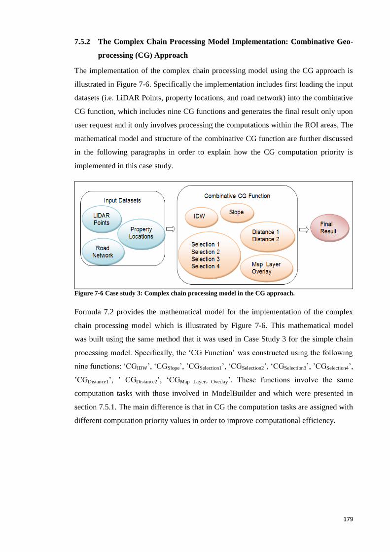
179
7.5.2 The Complex Chain Processing Model Implementation: Combinative Geo-
processing (CG) Approach
The implementation of the complex chain processing model using the CG approach is
illustrated in Figure 7-6. Specifically the implementation includes first loading the input
datasets (i.e. LiDAR Points, property locations, and road network) into the combinative
CG function, which includes nine CG functions and generates the final result only upon
user request and it only involves processing the computations within the ROI areas. The
mathematical model and structure of the combinative CG function are further discussed
in the following paragraphs in order to explain how the CG computation priority is
implemented in this case study.
Figure 7-6 Case study 3: Complex chain processing model in the CG approach.
Formula 7.2 provides the mathematical model for the implementation of the complex
chain processing model which is illustrated by Figure 7-6. This mathematical model
was built using the same method that it was used in Case Study 3 for the simple chain
processing model. Specifically, the ‘CG Function’ was constructed using the following
nine functions: ‘CGIDW’, ‘CGSlope’, ’CGSelection1’, ‘CGSelection2’, ‘CGSelection3’, ’CGSelection4’,
’CGDistance1’, ’ CGDistance2’, ‘CGMap Layers Overlay’. These functions involve the same
computation tasks with those involved in ModelBuilder and which were presented in
section 7.5.1. The main difference is that in CG the computation tasks are assigned with
different computation priority values in order to improve computational efficiency.

180
CG Function (CG dataset) = { CGMap Layers Overlay
{CGSelection1 (CGIDW (LiDAR Points))}
{CGSelection2 (CGSlope (CGIDW (LiDAR Points)))}
{CGSelection3 (CGDistance1 (Property Locations))}
{CGSelection4 (CGDistance2 (Road Network))}
(CG dataset)} [7.2]
The structure of the mathematical model is displayed in Figure 7-7 using different size
of blue dashed outline boxes which are used to illustrate how the CG functions are
organised. For example, the largest blue dashed outline box represents the ‘Map Layers
Overlay’ function, which aims to integrate the results from the four sub-functions, a, b,
c, d, which have different functionalities in the complex geo-processing model as it is
explained below:
a. {CGSelection1 (CGIDW (LiDAR Points))} // The main functionality is to select the
suitable area by the elevation value criterion.
b. {CGSelection2 (CGSlope (CGIDW (LiDAR Points)))} // The main functionality is to
select the suitable area by the slope value criterion.
c. {CGSelection3 (CGDistance1 (Property Locations))} // The main functionality is to
select the suitable area by the distance to existing property locations.
d. {CGSelection4 (CGDistance2 (Road Network))} // The main functionality is to select the
suitable area by the distance to the road network.
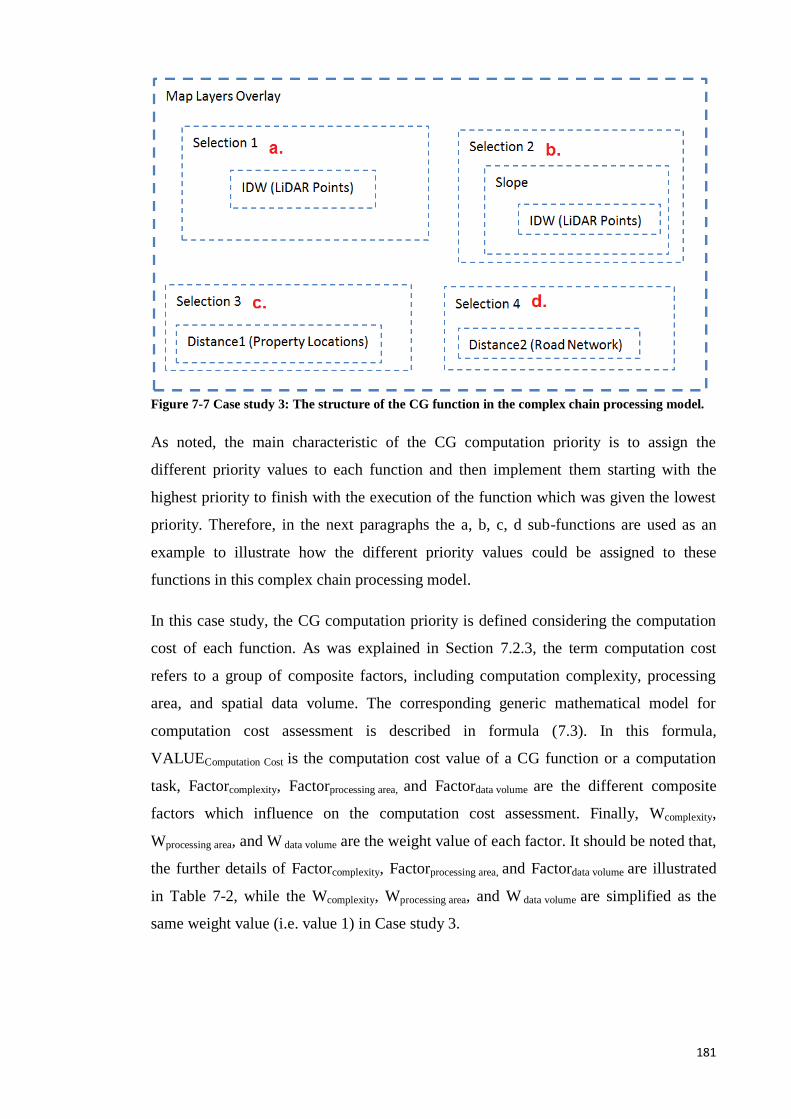
181
Figure 7-7 Case study 3: The structure of the CG function in the complex chain processing model.
As noted, the main characteristic of the CG computation priority is to assign the
different priority values to each function and then implement them starting with the
highest priority to finish with the execution of the function which was given the lowest
priority. Therefore, in the next paragraphs the a, b, c, d sub-functions are used as an
example to illustrate how the different priority values could be assigned to these
functions in this complex chain processing model.
In this case study, the CG computation priority is defined considering the computation
cost of each function. As was explained in Section 7.2.3, the term computation cost
refers to a group of composite factors, including computation complexity, processing
area, and spatial data volume. The corresponding generic mathematical model for
computation cost assessment is described in formula (7.3). In this formula,
VALUEComputation Cost is the computation cost value of a CG function or a computation
task, Factorcomplexity, Factorprocessing area, and Factordata volume are the different composite
factors which influence on the computation cost assessment. Finally, Wcomplexity,
Wprocessing area, and W data volume are the weight value of each factor. It should be noted that,
the further details of Factorcomplexity, Factorprocessing area, and Factordata volume are illustrated
in Table 7-2, while the Wcomplexity, Wprocessing area, and W data volume are simplified as the
same weight value (i.e. value 1) in Case study 3.
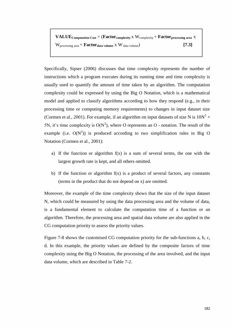
182
VALUEComputation Cost = (Factorcomplexity x Wcomplexity + Factorprocessing area x
Wprocessing area + Factordata volume x W data volume) [7.3]
Specifically, Sipser (2006) discusses that time complexity represents the number of
instructions which a program executes during its running time and time complexity is
usually used to quantify the amount of time taken by an algorithm. The computation
complexity could be expressed by using the Big O Notation, which is a mathematical
model and applied to classify algorithms according to how they respond (e.g., in their
processing time or computing memory requirements) to changes in input dataset size
(Cormen et al., 2001). For example, if an algorithm on input datasets of size N is 10N2 +
5N, it’s time complexity is O(N2), where O represents an O - notation. The result of the
example (i.e. O(N2)) is produced according to two simplification rules in Big O
Notation (Cormen et al., 2001):
a) If the function or algorithm f(x) is a sum of several terms, the one with the
largest growth rate is kept, and all others omitted.
b) If the function or algorithm f(x) is a product of several factors, any constants
(terms in the product that do not depend on x) are omitted.
Moreover, the example of the time complexity shows that the size of the input dataset
N, which could be measured by using the data processing area and the volume of data,
is a fundamental element to calculate the computation time of a function or an
algorithm. Therefore, the processing area and spatial data volume are also applied in the
CG computation priority to assess the priority values.
Figure 7-8 shows the customised CG computation priority for the sub-functions a, b, c,
d. In this example, the priority values are defined by the composite factors of time
complexity using the Big O Notation, the processing of the area involved, and the input
data volume, which are described in Table 7-2.
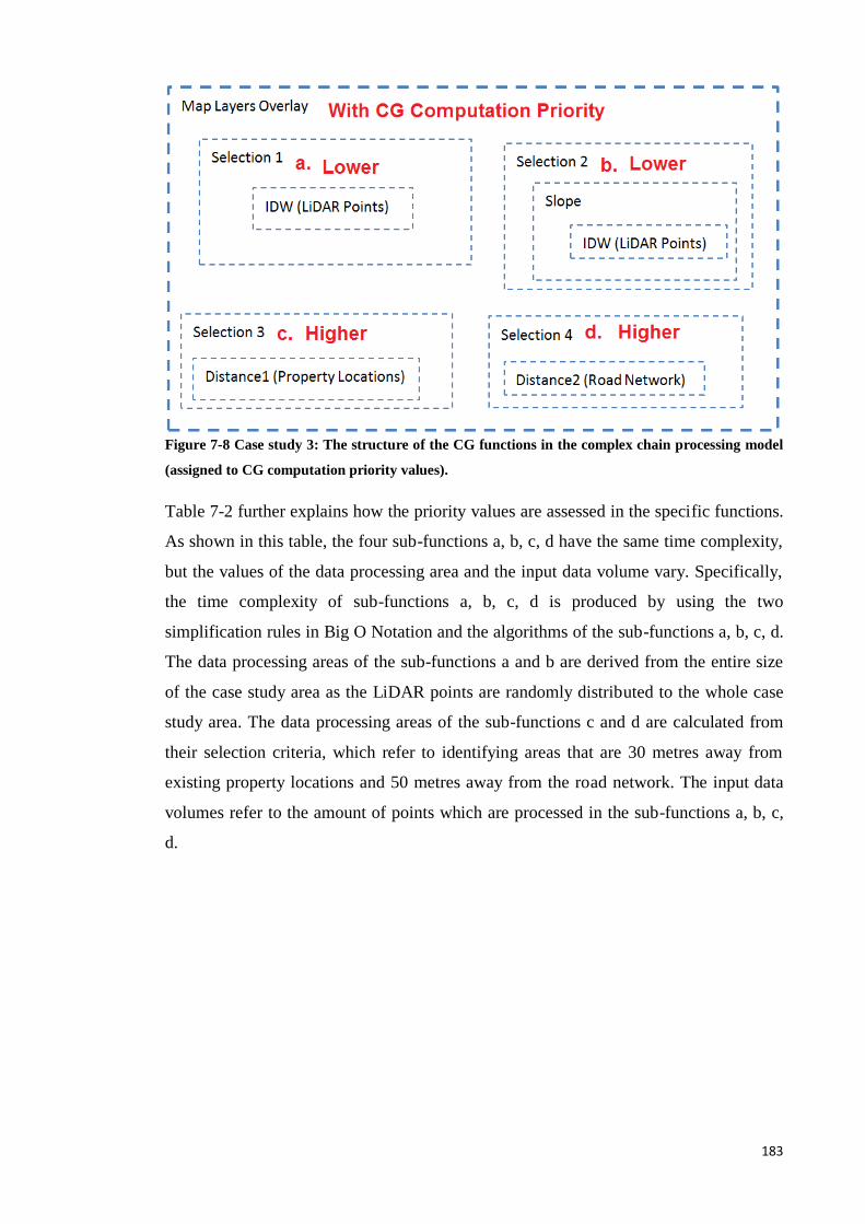
183
Figure 7-8 Case study 3: The structure of the CG functions in the complex chain processing model
(assigned to CG computation priority values).
Table 7-2 further explains how the priority values are assessed in the specific functions.
As shown in this table, the four sub-functions a, b, c, d have the same time complexity,
but the values of the data processing area and the input data volume vary. Specifically,
the time complexity of sub-functions a, b, c, d is produced by using the two
simplification rules in Big O Notation and the algorithms of the sub-functions a, b, c, d.
The data processing areas of the sub-functions a and b are derived from the entire size
of the case study area as the LiDAR points are randomly distributed to the whole case
study area. The data processing areas of the sub-functions c and d are calculated from
their selection criteria, which refer to identifying areas that are 30 metres away from
existing property locations and 50 metres away from the road network. The input data
volumes refer to the amount of points which are processed in the sub-functions a, b, c,
d.
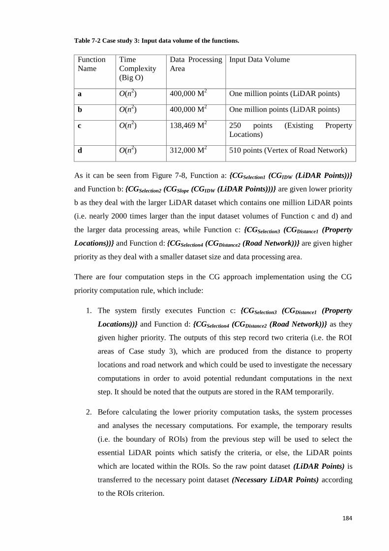
184
Table 7-2 Case study 3: Input data volume of the functions.
Function
Name
Time
Complexity
(Big O)
Data Processing
Area
Input Data Volume
a O(n2) 400,000 M
2 One million points (LiDAR points)
b O(n2) 400,000 M
2 One million points (LiDAR points)
c O(n2) 138,469 M
2 250 points (Existing Property
Locations)
d O(n2) 312,000 M
2 510 points (Vertex of Road Network)
As it can be seen from Figure 7-8, Function a: {CGSelection1 (CGIDW (LiDAR Points))}
and Function b: {CGSelection2 (CGSlope (CGIDW (LiDAR Points)))} are given lower priority
b as they deal with the larger LiDAR dataset which contains one million LiDAR points
(i.e. nearly 2000 times larger than the input dataset volumes of Function c and d) and
the larger data processing areas, while Function c: {CGSelection3 (CGDistance1 (Property
Locations))} and Function d: {CGSelection4 (CGDistance2 (Road Network))} are given higher
priority as they deal with a smaller dataset size and data processing area.
There are four computation steps in the CG approach implementation using the CG
priority computation rule, which include:
1. The system firstly executes Function c: {CGSelection3 (CGDistance1 (Property
Locations))} and Function d: {CGSelection4 (CGDistance2 (Road Network))} as they
given higher priority. The outputs of this step record two criteria (i.e. the ROI
areas of Case study 3), which are produced from the distance to property
locations and road network and which could be used to investigate the necessary
computations in order to avoid potential redundant computations in the next
step. It should be noted that the outputs are stored in the RAM temporarily.
2. Before calculating the lower priority computation tasks, the system processes
and analyses the necessary computations. For example, the temporary results
(i.e. the boundary of ROIs) from the previous step will be used to select the
essential LiDAR points which satisfy the criteria, or else, the LiDAR points
which are located within the ROIs. So the raw point dataset (LiDAR Points) is
transferred to the necessary point dataset (Necessary LiDAR Points) according
to the ROIs criterion.
185
3. The next step is to execute Function a: {CGSelection1 (CGIDW (Necessary LiDAR
Points))} and Function b: {CGSelection2 (CGSlope (CGIDW (Necessary LiDAR
Points)))}.
4. The last step is to run the ‘Map Layers Overlay’ function in the CG approach.
Sections 7.5.1 and 7.5.2 explained the two different approaches that can be used for the
implementation and execution of the complex chain processing model. The fundamental
difference is that in traditional geo-processing (i.e. ModelBuilder in ArcGIS) a
sequential computation method is used to process the model and its computation tasks,
while in the CG approach the CG functions are implemented based on their priority
values.
The following section discusses the input datasets that are used in Case study 3.
7.6 Case study 3: The Complex Chain Processing Model
Dataset
As it was already explained in Figure 7-4, the input datasets of Case study 3 include
LiDAR Points, property locations, and road network. They are separately described in
this section.
1) LiDAR Points (Case study 3)
The LiDAR Points are randomly selected from the original raw LiDAR dataset that also
used in the previous case study. It should be noted that there is a significant increase in
the number of LiDAR points used; from 26,666 points (i.e. the amount of LiDAR points
selected in Case Study 3) to 1,000,000 points. The purpose of using a large LiDAR
point dataset is to test and compare the overall computation time between the traditional
geo-processing approach and the CG approach, where CG computation priority is
further used. Figure 7-9 shows the sample of raw LiDAR point data used in this case
study, as well as, the geographical location and the topographical features of the study
area (shown by the yellow rectangle on top of the Bing Maps satellite image).
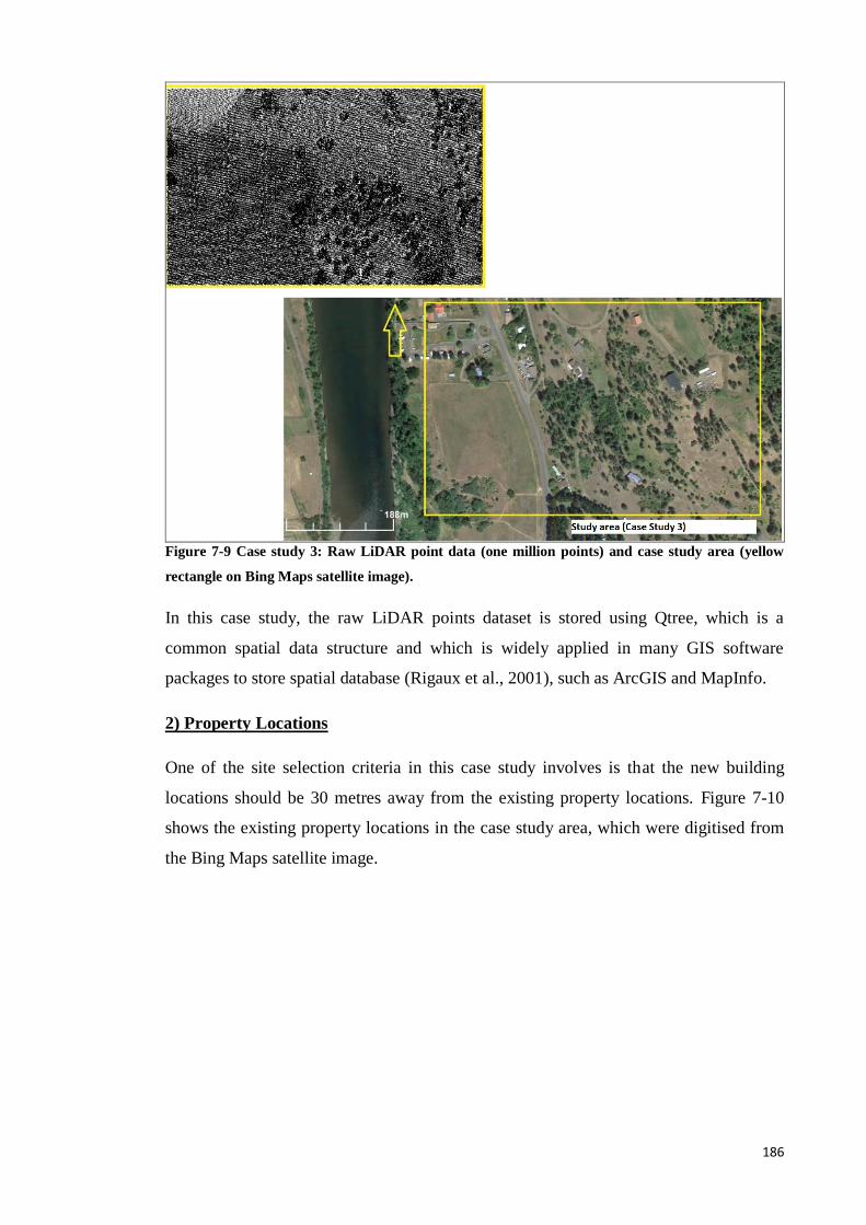
186
Figure 7-9 Case study 3: Raw LiDAR point data (one million points) and case study area (yellow
rectangle on Bing Maps satellite image).
In this case study, the raw LiDAR points dataset is stored using Qtree, which is a
common spatial data structure and which is widely applied in many GIS software
packages to store spatial database (Rigaux et al., 2001), such as ArcGIS and MapInfo.
2) Property Locations
One of the site selection criteria in this case study involves is that the new building
locations should be 30 metres away from the existing property locations. Figure 7-10
shows the existing property locations in the case study area, which were digitised from
the Bing Maps satellite image.
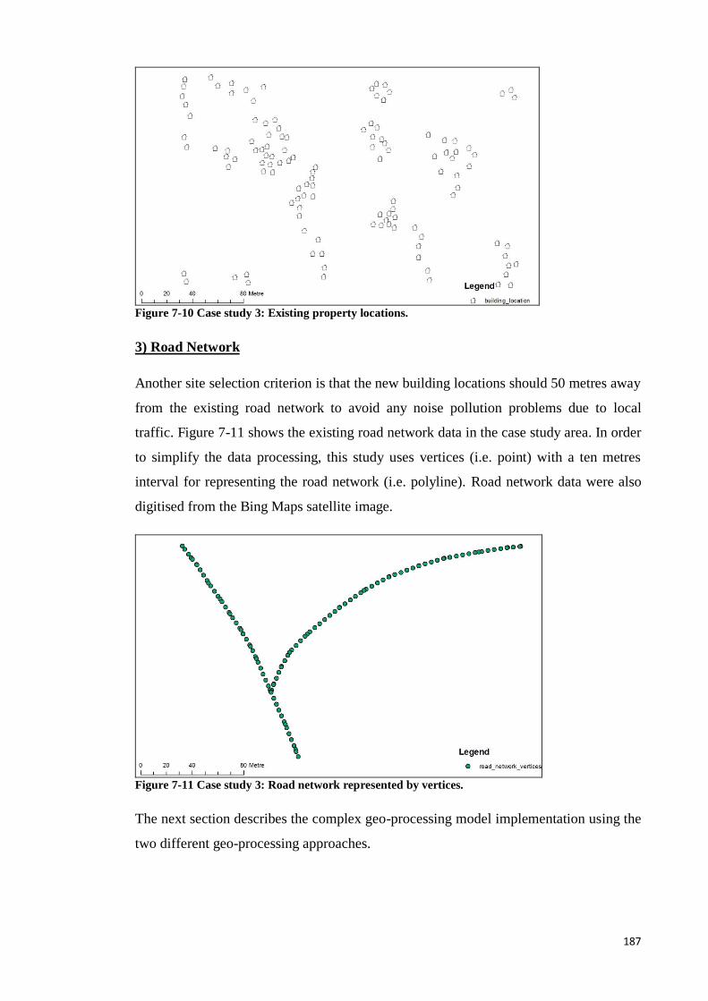
187
Figure 7-10 Case study 3: Existing property locations.
3) Road Network
Another site selection criterion is that the new building locations should 50 metres away
from the existing road network to avoid any noise pollution problems due to local
traffic. Figure 7-11 shows the existing road network data in the case study area. In order
to simplify the data processing, this study uses vertices (i.e. point) with a ten metres
interval for representing the road network (i.e. polyline). Road network data were also
digitised from the Bing Maps satellite image.
Figure 7-11 Case study 3: Road network represented by vertices.
The next section describes the complex geo-processing model implementation using the
two different geo-processing approaches.
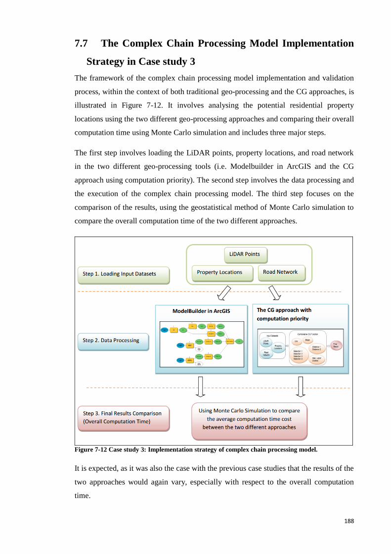
188
7.7 The Complex Chain Processing Model Implementation
Strategy in Case study 3
The framework of the complex chain processing model implementation and validation
process, within the context of both traditional geo-processing and the CG approaches, is
illustrated in Figure 7-12. It involves analysing the potential residential property
locations using the two different geo-processing approaches and comparing their overall
computation time using Monte Carlo simulation and includes three major steps.
The first step involves loading the LiDAR points, property locations, and road network
in the two different geo-processing tools (i.e. Modelbuilder in ArcGIS and the CG
approach using computation priority). The second step involves the data processing and
the execution of the complex chain processing model. The third step focuses on the
comparison of the results, using the geostatistical method of Monte Carlo simulation to
compare the overall computation time of the two different approaches.
Figure 7-12 Case study 3: Implementation strategy of complex chain processing model.
It is expected, as it was also the case with the previous case studies that the results of the
two approaches would again vary, especially with respect to the overall computation
time.
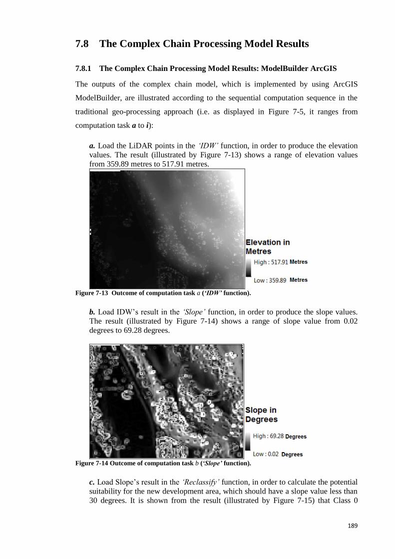
189
7.8 The Complex Chain Processing Model Results
7.8.1 The Complex Chain Processing Model Results: ModelBuilder ArcGIS
The outputs of the complex chain model, which is implemented by using ArcGIS
ModelBuilder, are illustrated according to the sequential computation sequence in the
traditional geo-processing approach (i.e. as displayed in Figure 7-5, it ranges from
computation task a to i):
a. Load the LiDAR points in the ‘IDW’ function, in order to produce the elevation
values. The result (illustrated by Figure 7-13) shows a range of elevation values
from 359.89 metres to 517.91 metres.
Figure 7-13 Outcome of computation task a (‘IDW’ function).
b. Load IDW’s result in the ‘Slope’ function, in order to produce the slope values.
The result (illustrated by Figure 7-14) shows a range of slope value from 0.02
degrees to 69.28 degrees.
Figure 7-14 Outcome of computation task b (‘Slope’ function).
c. Load Slope’s result in the ‘Reclassify’ function, in order to calculate the potential
suitability for the new development area, which should have a slope value less than
30 degrees. It is shown from the result (illustrated by Figure 7-15) that Class 0
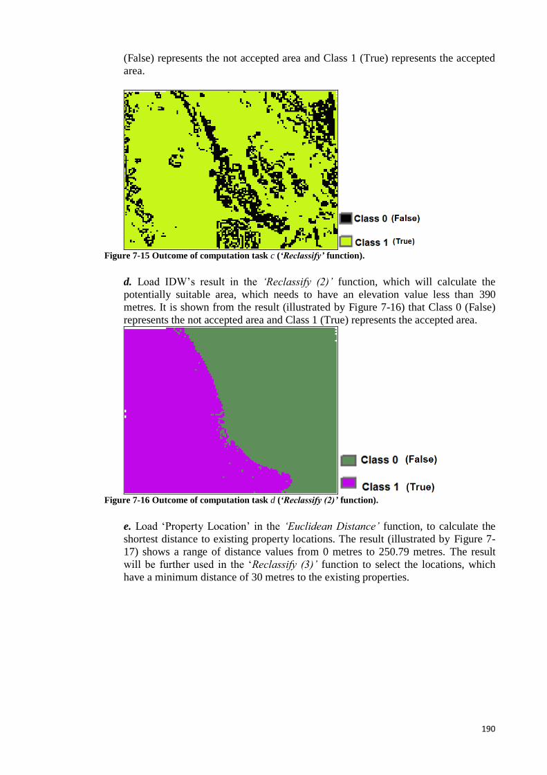
190
(False) represents the not accepted area and Class 1 (True) represents the accepted
area.
Figure 7-15 Outcome of computation task c (‘Reclassify’ function).
d. Load IDW’s result in the ‘Reclassify (2)’ function, which will calculate the
potentially suitable area, which needs to have an elevation value less than 390
metres. It is shown from the result (illustrated by Figure 7-16) that Class 0 (False)
represents the not accepted area and Class 1 (True) represents the accepted area.
Figure 7-16 Outcome of computation task d (‘Reclassify (2)’ function).
e. Load ‘Property Location’ in the ‘Euclidean Distance’ function, to calculate the
shortest distance to existing property locations. The result (illustrated by Figure 7-
17) shows a range of distance values from 0 metres to 250.79 metres. The result
will be further used in the ‘Reclassify (3)’ function to select the locations, which
have a minimum distance of 30 metres to the existing properties.
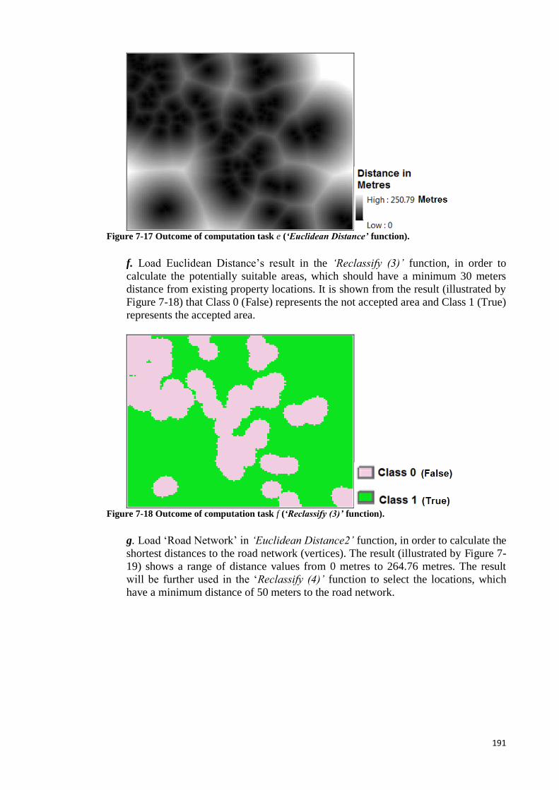
191
Figure 7-17 Outcome of computation task e (‘Euclidean Distance’ function).
f. Load Euclidean Distance’s result in the ‘Reclassify (3)’ function, in order to
calculate the potentially suitable areas, which should have a minimum 30 meters
distance from existing property locations. It is shown from the result (illustrated by
Figure 7-18) that Class 0 (False) represents the not accepted area and Class 1 (True)
represents the accepted area.
Figure 7-18 Outcome of computation task f (‘Reclassify (3)’ function).
g. Load ‘Road Network’ in ‘Euclidean Distance2’ function, in order to calculate the
shortest distances to the road network (vertices). The result (illustrated by Figure 7-
19) shows a range of distance values from 0 metres to 264.76 metres. The result
will be further used in the ‘Reclassify (4)’ function to select the locations, which
have a minimum distance of 50 meters to the road network.
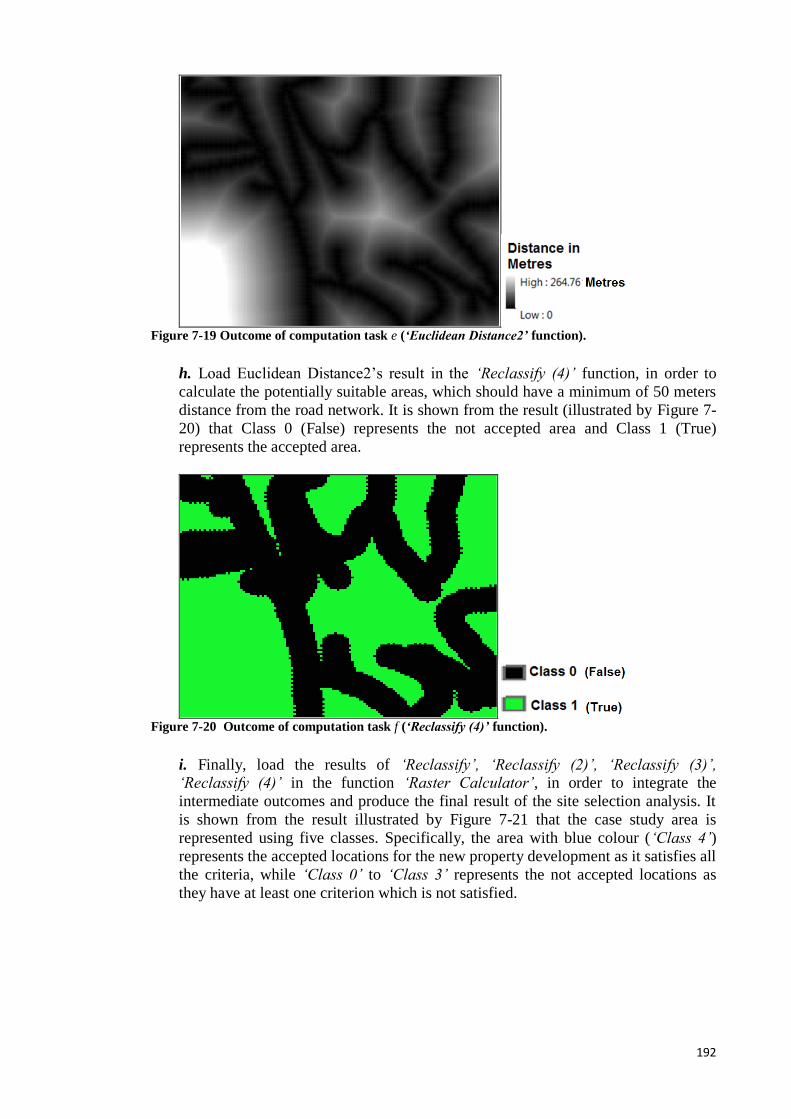
192
Figure 7-19 Outcome of computation task e (‘Euclidean Distance2’ function).
h. Load Euclidean Distance2’s result in the ‘Reclassify (4)’ function, in order to
calculate the potentially suitable areas, which should have a minimum of 50 meters
distance from the road network. It is shown from the result (illustrated by Figure 7-
20) that Class 0 (False) represents the not accepted area and Class 1 (True)
represents the accepted area.
Figure 7-20 Outcome of computation task f (‘Reclassify (4)’ function).
i. Finally, load the results of ‘Reclassify’, ‘Reclassify (2)’, ‘Reclassify (3)’, ‘Reclassify (4)’ in the function ‘Raster Calculator’, in order to integrate the
intermediate outcomes and produce the final result of the site selection analysis. It
is shown from the result illustrated by Figure 7-21 that the case study area is
represented using five classes. Specifically, the area with blue colour (‘Class 4’)
represents the accepted locations for the new property development as it satisfies all
the criteria, while ‘Class 0’ to ‘Class 3’ represents the not accepted locations as
they have at least one criterion which is not satisfied.
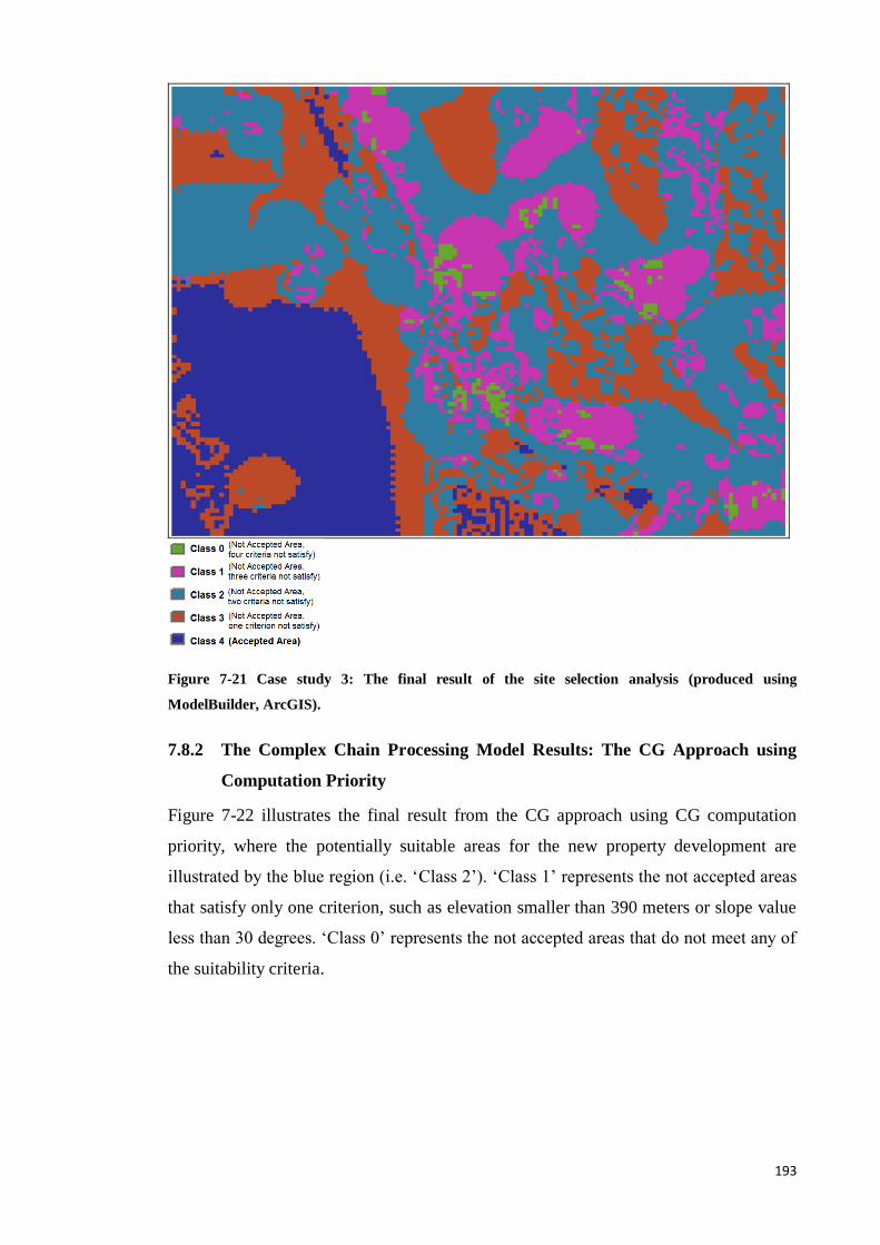
193
Figure 7-21 Case study 3: The final result of the site selection analysis (produced using
ModelBuilder, ArcGIS).
7.8.2 The Complex Chain Processing Model Results: The CG Approach using
Computation Priority
Figure 7-22 illustrates the final result from the CG approach using CG computation
priority, where the potentially suitable areas for the new property development are
illustrated by the blue region (i.e. ‘Class 2’). ‘Class 1’ represents the not accepted areas
that satisfy only one criterion, such as elevation smaller than 390 meters or slope value
less than 30 degrees. ‘Class 0’ represents the not accepted areas that do not meet any of
the suitability criteria.

194
Figure 7-22 Case study 3: The final result of the site selection analysis (produced using the CG
approach using CG computation priority).
Figure 7-22 shows that the entire case study area is divided by only three classes, as
opposed to the previous Figure 7-21 which illustrated the ArcGIS results and where
there were five classes. This is due to the new computation strategy (e.g. ROI), which is
applied in the CG approach. Specifically, as was explained in Section 7.2, ROI is used
to avoid the potential redundant computations in order to reduce the amount of
computation time. In this case study, when the site selection model is processed using
the CG approach with CG computation priority, the outcomes of the CG functions
{CGSelection3 (CGDistance1 (Property Locations))} and {CGSelection4 (CGDistance2 (Road
Network))} are applied to identify the boundary of ROIs, such as the regions which have
30 meters distance from existing property locations and also have 50 metres distance
from the road network. As a result, the computations are only implemented inside these
ROIs, and thus there are only three classes which are applied in the final result to further
investigate the other two criteria. They refer to the elevation values which should be
smaller than 390 meters and the slope value which should be less than 30 degrees.

195
Moreover, the white colour area displayed in the final result (Figure 7-22) represents the
locations, which did not involve any further processing as they are located outside the
ROIs.
This section presented the results of the complex chain processing model. The main
difference between the two approaches is that in the CG approach the final result is
directly produced, while the geographical data which is within the ROI are processed. In
contrast, the traditional geo-processing approach requires the sequential execution of all
the functions involved, which processes the data within the entire case study area.
7.9 Case study 3: Comparison of Results
We can now investigate the two different implementations of the complex chain
processing model with respect to their overall computation time. Monte Carlo
simulation is continuously applied in this case study to trace the average computation
time (i.e. mean value) of both geo-processing approaches.
7.9.1 Monte Carlo Simulation Model (Case study 3)
The Monte Carlo simulation model of this case study is given in Figure 7-23, which
involves three main steps:
1) The first step is to randomly select 90% of the LiDAR points as one of the input
datasets, which also include the property locations and the road network.
2) In the second step, the input datasets are loaded into the two different
approaches for data processing.
3) Finally, the average computation time of each approach is calculated and
compared.
It should be noted that the number of iterations used in the Monte Carlo simulation
model was increased to 100 iterations compared to the 50 iterations that were used in
the previous case study. The larger iteration number applied in this case study is due to
two reasons: (a) the amount of LiDAR data are gradually increased to one million points
from 26,499 points, which is the amount of LiDAR data used in the third case study; (b)
the geo-processing model applied in this case study is more complex than the one used
in Case Study 3 (i.e. the combinative function of ‘IDW’ and ‘Slope’). As a result, this
case study uses 100 iterations in the Monte Carlo simulation model. Moreover,
Heuvelink (2006) claims that 100 iterations are sufficient to obtain a reasonable
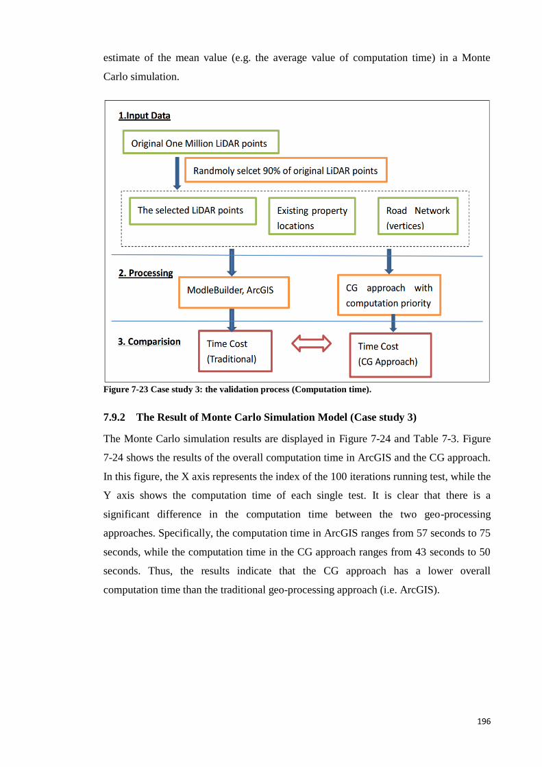
196
estimate of the mean value (e.g. the average value of computation time) in a Monte
Carlo simulation.
Figure 7-23 Case study 3: the validation process (Computation time).
7.9.2 The Result of Monte Carlo Simulation Model (Case study 3)
The Monte Carlo simulation results are displayed in Figure 7-24 and Table 7-3. Figure
7-24 shows the results of the overall computation time in ArcGIS and the CG approach.
In this figure, the X axis represents the index of the 100 iterations running test, while the
Y axis shows the computation time of each single test. It is clear that there is a
significant difference in the computation time between the two geo-processing
approaches. Specifically, the computation time in ArcGIS ranges from 57 seconds to 75
seconds, while the computation time in the CG approach ranges from 43 seconds to 50
seconds. Thus, the results indicate that the CG approach has a lower overall
computation time than the traditional geo-processing approach (i.e. ArcGIS).
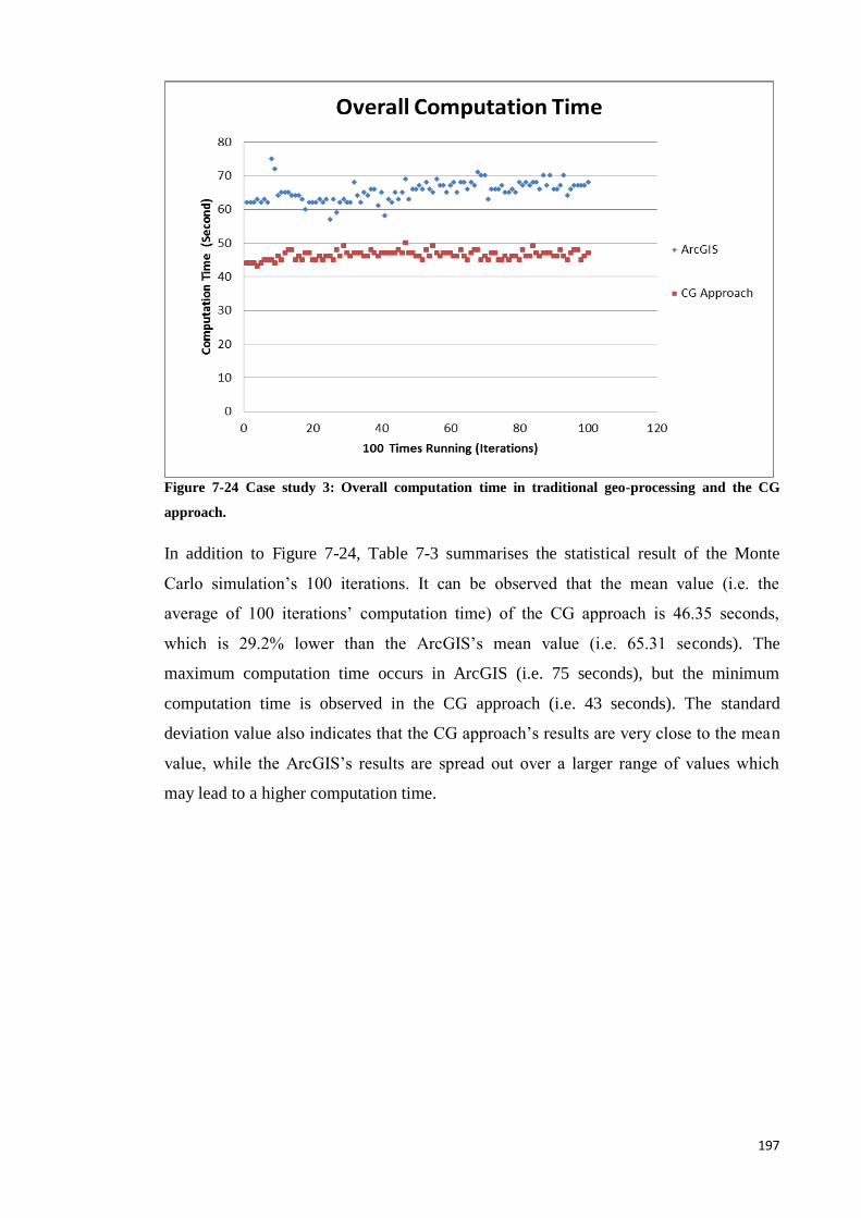
197
Figure 7-24 Case study 3: Overall computation time in traditional geo-processing and the CG
approach.
In addition to Figure 7-24, Table 7-3 summarises the statistical result of the Monte
Carlo simulation’s 100 iterations. It can be observed that the mean value (i.e. the
average of 100 iterations’ computation time) of the CG approach is 46.35 seconds,
which is 29.2% lower than the ArcGIS’s mean value (i.e. 65.31 seconds). The
maximum computation time occurs in ArcGIS (i.e. 75 seconds), but the minimum
computation time is observed in the CG approach (i.e. 43 seconds). The standard
deviation value also indicates that the CG approach’s results are very close to the mean
value, while the ArcGIS’s results are spread out over a larger range of values which
may lead to a higher computation time.
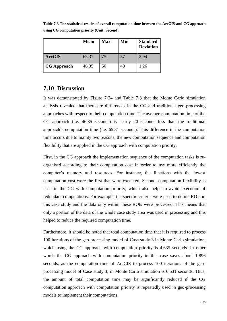
198
Table 7-3 The statistical results of overall computation time between the ArcGIS and CG approach
using CG computation priority (Unit: Second).
Mean Max Min Standard
Deviation
ArcGIS 65.31 75 57 2.94
CG Approach 46.35 50 43 1.26
7.10 Discussion
It was demonstrated by Figure 7-24 and Table 7-3 that the Monte Carlo simulation
analysis revealed that there are differences in the CG and traditional geo-processing
approaches with respect to their computation time. The average computation time of the
CG approach (i.e. 46.35 seconds) is nearly 20 seconds less than the traditional
approach’s computation time (i.e. 65.31 seconds). This difference in the computation
time occurs due to mainly two reasons, the new computation sequence and computation
flexibility that are applied in the CG approach with computation priority.
First, in the CG approach the implementation sequence of the computation tasks is re-
organised according to their computation cost in order to use more efficiently the
computer’s memory and resources. For instance, the functions with the lowest
computation cost were the first that were executed. Second, computation flexibility is
used in the CG with computation priority, which also helps to avoid execution of
redundant computations. For example, the specific criteria were used to define ROIs in
this case study and the data only within these ROIs were processed. This means that
only a portion of the data of the whole case study area was used in processing and this
helped to reduce the required computation time.
Furthermore, it should be noted that total computation time that it is required to process
100 iterations of the geo-processing model of Case study 3 in Monte Carlo simulation,
which using the CG approach with computation priority is 4,635 seconds. In other
words the CG approach with computation priority in this case saves about 1,896
seconds, as the computation time of ArcGIS to process 100 iterations of the geo-
processing model of Case study 3, in Monte Carlo simulation is 6,531 seconds. Thus,
the amount of total computation time may be significantly reduced if the CG
computation approach with computation priority is repeatedly used in geo-processing
models to implement their computations.
199
Although site selection geo-processing models are popular, it might be argued that these
models are not used by a significant amount of people so that also significant savings of
computation time occur due to the repetitive application of the proposed improved
approach in its existing form. However, it should be noted that the CG approach with
computation priority in its current form (i.e. without further research and subsequent
improvements) can be used in applications such as web mapping or online mapping,
which is used by thousands of people on a daily basis and which could significantly
improve computation time, as it is explained in the next paragraphs.
Web mapping provides a new way to design, implement, generate, and deliver
geographical information on the World Wide Web (Fu and Sun 2010). As web mapping
has many advantages, such as it could easily deliver information through internet
network, it can combine different data sources which are published online, and it could
work cross browsers and various operating systems to provide mapping services, while
there is a larger amount of users that are using web mapping services every day (Haklay
et at., 2008). In the early 2000s, the major characteristic of the web mapping is that geo-
processing functions can be executed on the powerful server’s side in order to process
geographical data and reduce in that way the computations that would be required to
execute on the client side (i.e. the user computer) (Peng and Tsou 2003). Then Google
Map applications which appeared in 2005, and the number of users is dramatically
increasing as Google Map applications provide a lot of convenient online map services.
For example, Google Maps API, which is a server side web mapping service, provides a
function to overlay user’s own data on a customized 2D Google Map, and Google Earth,
which is a client side web mapping service, offers a function to overlay user’s own data
on a customized 3D Google Map. Nowadays, Google Map applications are widely used
in various fields to implement different tasks, such as data visualisation, geo-processing
and spatial data integration.
If geo-processing functions are provided on web mapping services using the CG
approach with computation priority, significant computation time can be saved to the
service provider. For example, if the site selection geo-processing model implemented
using the CG approach in the Case study 3 is published on the server side for analysing
and sharing the information of potential property locations. The time saved could be
represented by ‘Number of Users’ times by ‘X seconds’, where ‘Number of Users’
describes how many people use this web mapping service and ‘X seconds’ means the
time saved of a single implementation. It might not be important for one user to save 20
200
seconds, which is based on the average computation time between the CG approach and
ArcGIS as demonstrated by Table 7.3, but for the provider it means that his the services
can save ‘Amount of Users’ x 20 seconds.
Therefore, based on the results of this case study and the earlier case studies (i.e. Case
Study 1 to 3), it can be concluded that the CG approach using computation priority
offers many advantages (i.e. improved data quality and better computation time) over
the traditional geo-processing approach for the implementation of a geo-processing
model.
7.11 Summary
This Chapter introduced the concept of CG computation priority, which was used in
order to improve the computational efficiency (i.e. the overall computation time) of geo-
processing. In the beginning, this Chapter reviewed the current problems related to
computational efficiency and introduced the concept of the CG computation priority.
Compared to the traditional geo-processing approach, the CG computation priority
provides an alternative computation strategy. Specifically, with the CG computation
priority the computation tasks or GIS functions of a geo-processing model are
implemented in a way that takes into account their computation cost, which is defined
by the size of the data involved and the computation complexity. In other words, the
function which involves a smaller data size and less complexity will be executed first.
The third case study focused on the implementation of a complex chain processing
model using the two different geo-processing approaches in order to demonstrate the
main characteristics of CG computation priority. The implementation results were
compared and it was found that the CG approach can produce the final result directly
and process the geographical data included in ROIs, while the implementation of
traditional geo-processing approach was executed sequentially and included processing
of the data within the entire case study area. The outcome of Monte Carlo simulation,
which was used to compare the computation time between two different geo-processing
approaches, confirms that the average of overall computation time in the CG approach
is 29.2% lower than the traditional geo-processing approach’s result. The results of
Monte Carlo simulation indicated that the CG approach using CG computation priority,
compared to the traditional geo-processing’s computation strategy, provides an
improved computation strategy for dealing with the complex geo-processing model and
the larger GIS datasets.
201
Although the CG approach with computation priority improved the computation time, it
may be argued that it only resulted in a very small fraction of computation time
reduction (around 20 seconds). Thus, it should be acknowledged that there are
additional concerns with respect to the implementation of CG computation priority.
It was explained in Section 7.3.2, the current method produces computation priority
values according to the composite factors, such as time complexity, processing area, and
input data volume. It should be noted that this current assessment progress may extend
the overall computation time as the composite factors are observed and evaluated one
by one until to produce a final priority value. Therefore, improving the speed of priority
value assessment is an important research question that should be addressed in the
further research, which does beyond the scope of this thesis, to further reduce the
overall computation time of geo-processing. For example, the computation priority
could be assessed by using an optimum computation algorithm, where the different
computation cost factors could be automatically and efficiently calculated.
The site selection geo-processing model was applied this this case study to demonstrate
how the CG approach with computation priority could be implemented. Moreover, the
site selection geo-processing model was used in the Monte Carlo simulation to validate
the computation time between the CG and traditional geo-processing approaches.
However, only a single geo-processing model implementation may not enough to
support the final conclusion of the new geo-processing approach if inappropriate inputs
were entered into the model, such as grid size and data volume. Therefore, various
implementation models are needed in the further CG approach development, although
these are beyond the scope of this thesis, to validate the performance of the CG
approach with computation priority.
202
8 Conclusion
8.1 Introduction
This thesis has described the development of a new geo-processing approach, the CG
approach, which was aimed at improving data processing issues related to data quality
and computational efficiency. Within this context, this thesis has described how the data
quality and computation time cost of geo-processing models can be optimised using the
CG approach. The research findings have been implemented and evaluated through
three test case studies, which focused on using the CG approach to optimise a set of
primitive geo-processing model implementations.
This chapter summarises the major findings of this research and discusses its
contributions, limitations and future research directions. Section 8.2 commences with a
brief overview of the research undertaken, whilst Section 8.3 discusses the research
questions of this thesis, and Section 8.4 discusses the contributions of this thesis.
Finally, the chapter concludes with a critical discussion of the limitations of the current
development of the CG approach (Section 8.5) and provides suggestions for future
research (Section 8.6).
8.2 Overview of the Research
This thesis has focused on the improvement of data quality and computational
efficiency in geo-processing. Although current geo-processing tools are used to model
and solve spatial decision-making problems, there are many significant concerns with
respect to the quality of their geo-processing results and the computational cost of a
geo-processing model. These were extensively described in Sections 2.3 and 2.4, where
the problems that are caused due to a sample’s resolution, the propagation of errors in
spatial information, and the extensive time cost were discussed. As the aim of this thesis
was to identify a solution in order to overcome these problems, a new geo-processing
approach was proposed which investigated how data quality problems can be minimised
and how computational efficiency, i.e. the overall computation time, of geo-processing
can be improved.
Chapter 2 reviewed geo-processing and the related issues, such as data quality and
computational efficiency. The data quality of a geo-processing model is extremely
important as it influences the final output of geo-processing models. Chapter 2 firstly
203
reviewed data quality issues in traditional geo-processing and then explained that the
current approach is influenced by different data quality problems, namely due to the
limitations of raster and vector spatial data models, and numerical computation and
error propagation. In order to minimise the spatial data representation problems and to
reduce data error and uncertainty, this research proposed the use of a point-based spatial
data model, i.e. spatial data representation, symbolic computation, and function-based
layers in the CG approach, i.e. data error and uncertainty. Chapter 2 also reviewed the
computational efficiency in geo-processing, as this can potentially influence
computational performance. The computation strategy, based on sequential computation
that it is used in traditional geo-processing, costs extra computation time and computer
memory. In order to address this problem, a priority-based computation strategy is
proposed in the CG approach, which is used to reduce computation time by re-ordering
the computational sequence in which the computation tasks in geo-processing are
implemented through the use of priority values from highest to lowest.
Chapter 3 introduced the conceptual model that links the main components of the CG
approach and it was explained that this conceptual model involves three parts: the first
focuses on the input level of the CG approach, such as the basic data model, functions,
and computation framework; the second part involves the processing and computation
rules that are used within the context of the CG approach; and the final part focuses on
the output level of the CG approach, such as the result of a geo-processing model. This
conceptual model of the CG approach provides the fundamental framework and the
basis for the development of the CG approach. Chapter 3 also discussed the two main
functionalities of the CG approach for executing spatial data and functions: (a) a CG
function, which can be constructed from sub-functions, is used to implement an entire
geo-processing model to reduce the impact of data errors and uncertainties; and (b) the
priority-based computation sequence, which is used to execute the CG functions
efficiently.
Chapter 4 discussed the case study design and the implementation of the methods. The
three case studies were introduced, which were implemented in order to demonstrate
how the CG function and the priority-based computation sequence could be practically
implemented using the CG approach, and further supported the investigation of whether
the CG approach improves data quality and computational efficiency. As the CG
function and priority-based computation sequence requires a set of implementation
methods, a ‘Higher-Order Function’, ‘Recursive Algorithm’ and ‘Lazy Evaluation’
204
were applied as the primary execution methods in the CG approach. The ‘Higher-Order
Function’ and ‘Recursive Algorithm’ can be used to build up and execute CG functions,
while ‘Lazy Evaluation’ can be applied to define the computational sequence.
Furthermore, the computational environment was also discussed in this chapter to
illustrate the software packages and computer tools which were used to implement the
three case studies.
The first case study was described in Chapter 5, and drew attention to the overlaying
raster layers in GIS. Due to the fact that this function is widely used by several geo-
processing models, e.g. for integrating different map layers in a complex geo-processing
model, this case study investigated and compared the computation strategy of the raster
layer overlay function. The second case study described in Chapter 6, showed how a
simple chain processing model can be implemented using the CG approach. This simple
chain processing model is a fundamental operation in traditional geo-processing, as it
forms the basis for building more complex geo-processing models. The last case study,
discussed in Chapter 7, demonstrated the implementation of a complex chain processing
model using the CG approach with computation priority, and also provided the basis to
further investigate the issue of computational efficiency in order to investigate how the
overall computation time cost in geo-processing can be reduced. Thus, in the third case
study, this thesis also introduced the concept of CG computation priority in processing
GIS data and functions. These three case studies are particularly important in the
development of the CG approach, especially for data quality and computational
efficiency improvement. The research findings from these three case studies are
discussed in the next section.
205
8.3 Overview of Research Objectives and Findings
This section discusses the major finding of the development of the CG approach,
specifically in relation to data quality improvement (Section 8.3.1) and computation
time optimisation (Section 8.3.2) which was one of the thesis aims.
8.3.1 Improving Data Quality via the Combinative Geo-Processing Approach
The research findings from case studies 1 and 2 illustrated that some fundamental
methods applied in the traditional geo-processing approach, such as spatial data
representation and the basic computation method, may influence data quality, due to: (a)
data conversion and re-sampling operations amongst raster and vector data models; and
(b) approximated values and error propagation during numerical and sequential
computation. It was concluded in Chapter 2 that the current spatial data representation
and the basic computation methods applied in the traditional geo-processing approach
can influence the data quality of the final results of a geo-processing model, and that
there is a need to improve the existing approach to provide a better result.
Addressing data quality problems was one of the main concerns in this research and was
an aspect of the CG approach at the conceptual and implementation levels. It was
discussed in Section 2.3 that there are two issues in the traditional geo-processing
approach, including the current method for spatial data representation and the basic
computation method, as these issues can cause different data quality problems. Two
case studies were undertaken in order to test the CG approach and to address these
problems. The findings of these case studies are discussed in the following paragraphs.
The first case study focused on the multiple raster map layers integration, which is a
common function commonly used in many geo-processing models and frequently
influences and causes data quality problems. A comparison between the CG approach
and the traditional geo-processing approach was demonstrated in the first case study
through implementing an overlay function of two different raster layers, with different
grid sizes. In particular, this case study involved the implementation of the raster layers
overlay function using the CG approach, ArcGIS, and MapInfo. The various results of
the raster layers overlay function were compared and it was found that the CG approach
resulted in values that were much closer to the observed values, i.e. the reference data.
As a result, it can be concluded that the CG approach offers an advantage over
traditional geo-processing for the integration of two or multiple raster map layers within
a geo-processing model.
206
The second case study also focused on data quality and was concerned with the
implementation of a simple chain processing model. A simple chain processing model is
central within geo-processing as it is used to build more complex and advanced models.
The second case study involved the implementation of a model using the CG approach
and the ModelBuilder tool provided by the ArcGIS software package. The
implementation results were compared using the Monte Carlo simulation method.
Monte Carlo simulations were used in this research to estimate standard deviation and
variance values of the samples, thereby enabling the tracking of the propagation of
uncertainties and errors of GIS computations. It was found that the CG approach
provided improved results, for example in the CG approach the average variance (7.304
degrees-squared) was nearly four times lower than the average variance in ArcGIS
(31.818 degrees-squared), in addition, the average standard deviation in the CG
approach (1.811 degrees) was nearly two times lower than the ArcGIS standard
deviation (3.844 degrees). The results of the Monte Carlo simulation indicated that the
CG approach results included less data uncertainty when compared to traditional geo-
processing, which is because the CG approach uses symbolic computation and function-
based layers for the execution of the various computational tasks.
To conclude, this research illustrates how the data quality of the traditional geo-
processing approach can be improved using the point-based spatial data representation,
symbolic computation and functional programming in the CG approach. In specific, the
point-based spatial data representation method improves the implementation of geo-
processing models as it reduces the complexity of spatial data models, while any
problems caused due to rasterisation and vectorisation of data processing functions can
be completely avoided. Furthermore, a combination of symbolic computation and
functional programming provides a novel approach in geo-processing for processing
spatial data and functions more accurately. There are many advantages to applying
symbolic computation and functional programming in the CG approach: first, both
numerical and symbolic computations are supported in the CG approach to reduce the
influence of an approximated value; second, computations can be suspended or
reordered in order to implement them more efficiently; and third, results can be
produced directly from a combination of functions thereby reducing data uncertainty.
Furthermore, the point-based spatial data representation, symbolic computation and
functional programming in the CG approach can contribute to many further contexts
within GIS, such as point cloud geo-data and geocomputation and these contributions
are discussed further in Section 8.4.

207
Apart from the data quality investigation, this thesis has also explored how
computational efficiency, i.e. overall computation time, can be improved when the CG
approach is applied in geo-processing. The findings of this investigation are separately
summarised in the next section.
8.3.2 Improving Computational Efficiency through the Combinative Geo-
Processing Approach
The sequential computation strategy applied in the traditional geo-processing approach
is another issue, as it could result in problems related to computational efficiency. A
common problem is that all functions need to wait for input data from the previous
functions, and also unnecessary computations may occur in a complex geo-processing
model. Together, these two problems can potentially increase the computational cost of
geo-processing models. Thus, it may be concluded that the sequential computation
sequence can influence the computational efficiency of a geo-processing model, and
that there is a need to improve the existing approach in order to reduce the computation
cost.
The computational efficiency problems in the traditional geo-processing approach have
influenced the development of the CG approach. In order to reduce the total
computation time, the design of the CG approach has focused on improving the
sequential computation in the traditional geo-processing approach by using a priority-
based computation strategy. The priority-based computation strategy attempts to
overcome the problem of overall computation timeof geo-processing, especially when
large spatial datasets and complex geo-processing models are involved. The priority-
based computation strategy enables an alternative computation sequence to execute GIS
functions in a geo-processing model, which is achieved by initially assigning
computation tasks with different priority values, and then implementing them according
to this priority value, from highest to lowest.
The third case study showed how the CG approach with the priority-based computation
strategy can be implemented in a complex chain processing model. The model was
implemented using the traditional approach (ModelBuilder in ArcGIS) and the CG
approach with computation priority in order to compare the computation time costs of
the two approaches. The implementation results revealed that the CG approach can
produce the final result directly, i.e. without any interim outputs, and process
geographical data included in ROIs, while the implementation of the traditional geo-
208
processing approach was executed sequentially and included processing of the data
within the entire case study area. Furthermore, a Monte Carlo simulation was used in
this case study to compare the average of the overall computation time (based on 100
iterations) between the two different geo-processing approaches. The outcome of the
simulation confirmed that the average overall computation time in the CG approach is
29.2% lower than in the traditional geo-processing approach. The results indicated that
the CG approach using computation priority, compared to the traditional geo-processing
computation strategy, provides an improved computation strategy for dealing with
complex geo-processing models and larger GIS datasets.
To summarise, this research has illustrated how the computational efficiency of the
traditional geo-processing approach can be improved using the priority-based
computation strategy employed in the CG approach. Moreover, the priority-based
computation strategy could create more contributions to high-performance
geocomputations and daily geo-processing tasks, as it enables an efficient way to
process GIS data and functions. The further contributions of the priority-based
computation strategy are discussed in Section 8.4.
8.4 Contribution of Thesis
This thesis contributes to the area of geo-processing, which is a popular approach in
GIS and has been widely used in various spatial analysis tasks. Specifically, it
introduces novel thinking and an approach to the field of geo-processing computations,
such as using function-based layers and a priority-based computation strategy to process
GIS data and functions. Based on the previous discussion of the research findings, the
primary contribution of the research undertaken can be concluded as: (a) the
development of a new approach for processing GIS data and functions; (b) a
demonstration of how the influence of data errors and uncertainties in geo-processing
can be minimised using a point-based spatial model and a combination of symbolic
computation and function-based layers; and (c) a demonstration of how the overall
computation time of geo-processing can be improved using the priority-based
computation strategy. The contributions of this thesis to different GIS research areas are
discussed in the following paragraphs.
The point-based spatial data model provides a simplified way to represent spatial
features. In other words, the CG approach uses point data to represent spatial features
that include both discrete objects and continuous field features. It should be noted that a
209
point-based spatial data model is not a new concept in GIS, as it is usually used to
represent individual point objects in a geo-processing model, such as address points.
However, this is the first time a point-based spatial data model has been used to
represent both discrete and continuous data in a geo-processing model in order to reduce
the influence of data quality issues, such as rasterisation and vectorisation.
Furthermore, the contribution of the point-based spatial data model has an important
implication for the analysis of large point cloud geo-data. Point cloud geo-data are
defined as X, Y, and Z coordinates within a geographical coordinate system, and aim to
represent spatial objects, such as three-dimensional buildings (Höfle et al., 2009). Point
cloud geo-data have been applied in different applications in order to represent spatial
objects, for example, Oude and Vosselman (2009) stated that three dimensional
modelling of complex highway interchanges could be represented using point cloud
geo-data. In addition, Hentschel and Wagner (2010) discussed that Points Of Interests
(POI), such as traffic signs, gas stations and restaurants, could be represented using
point cloud geo-data.
Although point cloud geo-data are increasing in popularity, there are some existing data
quality issues which may cause problems. In particular, Pauly et al. (2004) illustrated
the data uncertainty and variability issues which exist in point cloud geo-data due to
incomplete information captured by 3D acquisition devices. Joerg et al. (2012)
discussed point cloud geo-data collected from different airborne sensors which are often
integrated together to build a complete database, where massive point cloud data
captured from different platforms and sensors create potential data quality problems for
data integration and manipulation. If the point-based spatial data model in the CG
approach could be applied to point cloud geo-data, then it will reduce the influence of
data uncertainty and error propagation in point cloud geo-data processing and improve
GIS representations.
The CG approach introduces a completely different way to process GIS data and
functions using function-based layers. The basic idea of function-based layers was
discussed in Section 3.3 and based on the first and second case studies, it was found that
function-based layers provided a way to improve the data quality of geo-processing. For
example, the influence of data uncertainties, e.g. error propagation and spatial data
conversion, could be minimised by using symbolic computation and function-based
layers in the CG approach, and increased flexibility was also provided in the CG
210
approach as the resolution and extent of the output could be defined by the users
according to a request.
The contribution of function-based layers has an important implication for improving
the data quality of geocomputation. Geocomputation is an approach that it is used for
interpreting spatial characteristics, explaining geographical phenomena, and solving
spatial problems (Couclelis, 1998; Cheng et al., 2012). Nowadays, geocomputation is
widely applied in various fields to understand complex geographical phenomena, such
as health data analysis (Câmara and Monteiro, 2001) and geodemographics (Ashby and
Longley, 2005). It should be noted that spatial data quality improvement is an ongoing
topic in geocomputation due to many existing issues which were discussed in Section
2.3.3, such as data transformation and error propagation. If the function-based layers in
the CG approach could be applied to geocomputation, then this will enable a different
way to manipulate GIS data and functions and reduce the influence of data uncertainties
and errors in geocomputation.
Aside from data quality, this thesis has also paid attention to the overall computation
time through the concept of CG computation priority. It is particularly important to note
that this is probably the first time priority values have been applied to GIS functions in
order to improve computational efficiency. In contrast to the computation strategy of the
traditional geo-processing approach, a more sophisticated variant of the CG
computation priority is that each GIS function has a priority value derived from the
particular computation cost, which is used to execute the available functions from
highest to lowest priority. As a result, the overall computation time of geo-processing
can be reduced, as the new approach enables a way to use computer resources
efficiently and avoid redundant computations.
The novel CG computation priority has an important implication for improving the
performance of geo-processing. Nowadays, many geo-processing research studies relate
to high performance computation, such as parallel computation. For example, Dowers et
al. (2000) suggested a framework and a series of software libraries, which allow the
integration of parallel computation technology into the GIS software to improve
computational efficiency. Parallel computation has two benefits for implementing multi-
computational tasks in a geo-processing model; first, it supports an efficient platform to
encompass a wider range of complex processes in a geo-processing model, which can
be divided and achieved by multi-streaming sequential geo-processing tasks across
different cores (Qin et al., 2014); and second, it enables a new platform to store the
211
ocean of GIS data which are collected from spatial and temporal dimensions (Zhong et
al., 2012). However, it should be noted that parallel computation focuses on how heavy
computational tasks can be efficiently divided into smaller computational tasks via the
use of a multi-core processor. This characteristic indicates that: (a) parallel computation
doesn’t change the sequential computation strategy in the traditional geo-processing
approach; and (b) the problems related to sequential computation strategy still exist in
parallel computation. These issues raise several questions for future research, such as
can parallel computation be applied in the CG approach and can the priority-based
computation strategy be integrated into the parallel computation? Although the
integration between the two methods may further reduce the overall computation time
of a geo-processing model, this integration also has some potential challenges in future
development. For example, how could a combinative function divided into sub-
computation tasks and how are sub-computation tasks prioritised in parallel
computation?
The contribution of the CG approach could be further extended to several research
contexts, e.g. environmental modelling, web mapping services, urban planning, risk
assessment, or asset management, as it fundamentally improves geo-processing. People
currently work in many different fields and use geo-processing models to solve many
spatial problems. For example, scientists use geo-processing models to monitor and
analyse daily atmospheric changes, such as temperature and air pollution, biologists use
geo-processing models to track animal migration patterns, city planners and engineers
use geo-processing models to help plan their response in the case of a natural disaster,
such as an earthquake or hurricane and engineers and specialists use geo-processing
models to plan local resources needed for energy services, like gas and electricity.
Therefore, there are many potential opportunities for the CG approach to be applied to
different fields in order to improve data quality and computational efficiency.
Last but not least, if the CG approach could be frequently and repeatedly used in Web
GIS and online geo-processing, further computation time and computer resources could
be saved. It should be noted that the current geo-processing tool, not only could be used
in different GIS desktop software packages (e.g. ERDAS and ArcGIS) for spatial
analysis and decision-making, but also has been widely and repeatedly applied in Web
GIS and online geo-processing to support spatial data processing and map publishing
services. Niu et al. (2013) discussed how geo-processing services could be provided
using Web GIS and concluded that online geo-processing provides a convenient way to
212
reduce the differences between platforms and programming languages, but that
computational efficiency is a potential problem for online geo-processing and requires
further investigation. Another example is Google Map applications which appeared in
2005, where the number of users dramatically increased as Google Map applications
provide convenient online mapping services. If the popular online data processing
functions that are repeatedly applied in GIS users’ daily jobs could be implemented
using the CG approach, then there are significant computation times that could be saved
for web service providers and potential contributions that could be made for different
web mapping service users. For example, the overlay of map layers and potential site
selection, which were discussed in Chapters 5 and 7, are two popular functions and have
been widely applied in online geo-processing. If these functions could be implemented
using the CG approach, then this would improve data quality and the computational
efficiency of online geo-processing.
The next section discusses the limitations of the CG approach.
8.5 Research Limitations
In this thesis different methods were used to develop the CG approach. For example, a
conceptual model was discussed at the beginning of the thesis to build the framework
for the development of the CG approach, then there are the three case studies that were
applied to the CG approach implementation, and finally a geostatistical method (i.e. a
Monte Carlo simulation) was used to trace the uncertainties, e.g. data quality and
computation time cost, and evaluate the results of the case studies. These different
methods, which each have their own limitations, were applied to answer the research
question of this thesis and therefore they are critically discussed in this section.
8.5.1 Conceptual Model of the Combinative Geo-Processing Approach
The conceptual model of the CG approach was discussed in Chapter 3 in order to
explain the major characteristics of the new approach, and this model plays an important
role in the three case studies that were used for the development of the CG approach.
However, it should be noted that there are some limitations with respect to the
implementation of the conceptual model in the current CG approach, which mainly refer
to the CG function library and the CG function output visualisation.
First, there is a barrier for many GIS users in comprehending the performance gains
delivered by the CG approach because of the limited amount of CG functions and geo-
213
processing models that were implemented in the development of the CG approach. As
was discussed in Section 3.3, the CG function library is a core element in the input level
of the CG conceptual model for storing and managing different CG functions
effectively. CG functions can be developed and stored in the CG function library, and
subsequently these functions were used in the case studies for the implementation of the
CG approach. However, due to time restrictions, only a basic set of CG functions was
created in the library for test purposes. Therefore, further research is required to expand
the diversity of the functions that are included in the CG function library so that the
approach will be eventually used to implement various CG functions and geo-
processing models in different fields.
Second, although the CG approach provides flexibility regarding the data formats of the
output level, it should be noted that there is a potential limitation with respect to data
visualisation. Specifically, the results of the current CG approach need a further step to
enable data visualisation. For example, if users want to display the CG approach result
in raster format, then a point list data need to be converted using the ‘ASCII to raster’
function. Therefore, the CG approach would ideally require the development of a
graphical user interface (GUI) to solve this limitation of data visualisation. This
potential GUI of the CG approach would provide greater flexibility for data
visualisation, as it could display the same list point data in various data formats (e.g.
raster, vector, 3D). Moreover, as the CG approach can produce a function or functions
for the results, then the GUI of the CG approach also needs to provide the ability to
display these functions. For instance, instead of displaying raster or vector data, the GUI
of the CG approach could visualise the function-based layers and their manipulation
progress.
8.5.2 Design of Case Studies
Three different case studies were applied in this thesis for the development of the CG
approach. These case studies have different limitations and implications, which are
critically discussed in this section.
Although the results of case study 1 showed that the CG approach improved the results,
especially when compared with the traditional raster layer overlay method in map
algebra, it may still receive some criticism as the geo-processing model implementation
involves a simple model which requires the integration of only two raster layers. Thus, a
chain processing model, including two different GIS functions (IDW and Slope) was
214
introduced in case study 2 in order to increase the complexity of the implementation
model. In addition, the case study area and the sample data volume were gradually
increased in case study 2 to validate the result of the CG approach.
Case study 2 showed how a combinative function (IDW and Slope) can be implemented
using the CG approach. This case study can also be criticised with respect to the large
amount of computation time that was required by both geo-processing approaches.
Although this was mainly due to the large amount of sample data that were applied in
case study 2, it is still evident that the existing geo-processing approaches, i.e. the CG
approach without computation priority and the traditional geo-processing approach, do
not encapsulate an efficient computation strategy that can be used to deal with large
spatial data and complex computations. In order to overcome this limitation CG
computation priority was introduced in the next case study to improve the overall
computation time.
The objective of case study 3 was to develop the computational priority rule of the CG
approach in order to improve the overall computation time. Although the final results
showed that the average overall computation time in the CG approach with computation
priority is 29.2% (around 20 seconds) lower than for the traditional geo-processing
approach, this case study may subject to several criticisms. Case study 3 only resulted in
a very small reduction in computation time (around 20 seconds) and it may not convince
GIS users to use the CG approach with computation priority to execute their geo-
processing tasks. Yet it is essential to highlight that if the CG approach with
computation priority is used in geo-processing tasks which are frequently applied in
daily jobs, such as web mapping services, then significant computation time can be
saved for web mapping service providers, such as Google Maps and Bing Maps.
The speed of computation priority assessment in the current CG computation priority
rule is not efficient, as the composite factors of computation priority are observed and
evaluated one by one until a final priority value is produced. Improving the speed of the
priority value assessment is an important research question that requires further
investigation in order to reduce the overall computation time of geo-processing.
Finally, there is only one geo-processing model, i.e. the site selection model, that was
applied in case study 3, and thus various additional implementation models are required
to further validate the performance of the CG approach with computation priority.
215
8.5.3 Data Validation Method (Monte Carlo Simulation)
A Monte Carlo simulation was used in this research to evaluate the uncertainties of the
final results. A Monte Carlo simulation was applied in case study 2 to calculate the
mean and variance of the results in order to investigate the influence of data
uncertainties in the simple chain processing model implementation. Furthermore, a
Monte Carlo simulation was applied in case study 3 to trace the average computation
time, i.e. mean value, of both geo-processing approaches. Although a Monte Carlo
simulation provides a useful method to trace the uncertainties and compare the results of
the CG and the traditional geo-processing approaches, it should be noted that a Monte
Carlo simulation has two limitations with respect to the iteration times and input data,
and these problems are discussed in more detail in the remainder of this section.
The first limitation in a Monte Carlo simulation is the numerical load or computation
iterations, as the operation must be executed ‘N’ times. Heuvelink (2006) argued that
the iteration time N is a limitation of a Monte Carlo simulation mainly due to two
reasons: a) if a small number of iterations is applied in a Monte Carlo simulation, then
the simulation can lead to misleading results as there are not enough computations; and
b) if a larger number of iterations is applied then this may lead to heavy computations.
These limitations therefore draw attention to the question of how many iterations should
be used in the case studies presented in this thesis. This problem was discussed for both
case studies 2 and 3 in order to identify a suitable number of computation iterations.
Most GIS studies run a Monte Carlo simulation with only 20 or even ten iterations
(Fisher, 1999; Goodchild et al., 1992), although Goodchild et al. (1992) claimed that ten
or twenty iterations are not sufficient to obtain an accurate estimation of the results.
Furthermore, Heuvelink (2006) suggested that in most cases a Monte Carlo simulation
should include at least 50 computation iterations. Therefore, case study 2 used 50
iterations in order to provide an accurate estimation of the influence of data
uncertainties. In contrast, case study 3 used 100 iterations, for two main reasons: a) the
amount of LiDAR data were gradually increased to one million points from 26,499
points, which is the amount of LiDAR data used in the third case study; and (b) the geo-
processing model applied in this case study is more complex than the one used in case
study 2, i.e. the combinative function of ‘IDW’ and ‘Slope’. Moreover, Heuvelink
(2006) claimed that 100 iterations are sufficient to obtain a reasonable estimate of the
mean value (e.g. the average value of computation time) in a Monte Carlo simulation.
216
The second limitation of a Monte Carlo simulation is the input datasets, as simulations
can lead to misleading results if inappropriate inputs are entered into the model
(Ibbotson Associates, 2005). For instance, a small sized input dataset in a Monte Carlo
simulation is not enough to support the outcomes based on statistical analysis (e.g. mean
and standard deviation values) because the outputs may be totally changed based on
different small sized datasets. This problem was investigated in Section 4.4, and the size
of the sample dataset was gradually increased in the three case studies. For example,
case study 2 used 26,000 points from the original LiDAR dataset, whereas in case study
1 1,000 points were selected from the original LiDAR dataset and in case study 3 one
million LiDAR points were used to validate the overall computation time between the
two different geo-processing approaches.
The next section discusses the future research directions for the CG approach.
8.6 Directions For Future Research
The CG approach was developed based on a limited number of sample data and case
studies due to the complexities of model development and the limitations regarding time
and knowledge. Therefore, a future research is requested to extend the functionalities
and contributions of the CG approach. This section summarises some interesting
directions for the future research.
a. Advancing the Combinative Geo-Processing Function Library
An ideal geo-processing approach needs to be supported by sufficient GIS functions,
(i.e. different types of function libraries, such as the ModelBuilder in the ArcGIS
software package which offers thousands of functions in its Toolbox in order to provide
a powerful means of GIS modelling. However, only a basic set of common GIS
functions was developed in the current CG function library due to time restrictions.
Future research should also extend the development of more CG functions as part of the
CG function library, in order to enhance the functionality and capability of the CG
approach for a wider spectrum of GIS applications, e.g. 3D land surface models,
weather temperature prediction models, hydrological models, and environmental risk
assessment models.
b. Combinative Geo-processing Computation Priority
This thesis introduced the concept of CG computation priority as a solution for reducing
the overall computation time of geo-processing. However, the current method for
assessing computation priority is very slow and could extend the overall computation
217
time. Therefore, improving the speed of the priority value assessment is an important
research area that should be addressed in the future to further reduce the overall
computation time of geo-processing. Future research should focus on identifying an
efficient method that can assess the computation priority value through the design of an
optimum computational algorithm to address this problem and its implementation.
Furthermore, as was discussed in Section 8.4, in future research CG computation
priority may be applied to parallel computation in order to further improve
computational efficiency.
c. Developing New Combinative Geo-Processing Computation Rules
To date three computation rules have been introduced into the CG approach to improve
data quality and computation time, and these include ‘suspending’, ‘computation
priority’, and ‘symbolic computation’ (see Section 3.3.2). New computation rules could
be developed in future research to further enhance the performance of the CG approach.
For instance, the CG approach is in need of a reduction rule to simplify complex geo-
processing models which are constructed of various function-based layers or CG
functions. Therefore further investigation is needed to create a reduction rule in the CG
approach to improve computational efficiency. A reduction rule based on the function-
based layers should also be created to understand how data quality can be maintained
during the reduction operations.
In conclusion, this thesis has used the CG approach to implement different types of geo-
processing models, e.g. a single GIS function, a simple chain processing model, and a
complex chain processing model. The results of the case studies show that the CG
approach provides an improved methodology for geo-processing. Future investigations
should focus on the improvement of CG computation rules, e.g. the reduction rule and
the computation priority rule, and the enhancement of the CG function library, as these
will further improve the performance of the CG approach and increase the potential
number of users of the CG approach in wider GIS applications. It is hoped that this
approach will continue to be developed in order to provide more accurate and efficient
results for various geo-processing models in different GIS fields.
218
Reference
Aji, A., Wang, F. and Saltz, J.H., 2012. Towards building a high performance spatial
query system for large scale medical imaging data. In Proceedings of the 20th
International Conference on Advances in Geographic Information Systems (pp.
309-318). California, USA, November 6-9 2012. ACM.
Almeida, L.P., Ferreira, Ó. and Taborda, R., 2011. Geoprocessing tool to model
beach erosion due to storms: application to Faro beach (Portugal). Journal of
Coastal Research, (64), p.1830.
Ansola, R., Canales, J. and Tárrago, J.A., 2006. An efficient sensitivity computation
strategy for the evolutionary structural optimization (ESO) of continuum
structures subjected to self-weight loads. Finite elements in analysis and
design, 42(14), pp.1220-1230.
Arbia, G., Griffith, D. and Haining, R., 1998. Error propagation modelling in raster
GIS: overlay operations. International Journal of Geographical Information
Science, 12(2), pp.145-167.
Arts, D.G., De Keizer, N.F. and Scheffer, G.J., 2002. Defining and improving data
quality in medical registries: a literature review, case study, and generic
framework. Journal of the American Medical Informatics Association, 9(6),
pp.600-611.
Ashby, D.I. and Longley, P.A., 2005. Geocomputation, geodemographics and
resource allocation for local policing. Transactions in GIS, 9(1), pp.53-72.
Beard, K., 1989. Use error: the neglected error component. In Proceedings of Auto-
Carto (Vol. 9, pp. 808-817). Baltimore, Maryland, April 2 - 7, 1989. Auto-
Carto.
Biljecki, F., Ledoux, H. and Stoter, J., 2014. Error propagation in the computation of
volumes in 3D city models with the Monte Carlo method. ISPRS Annals of the
Photogrammetry, Remote Sensing and Spatial Information Sciences, 2(2), p.31.
Bingham, L. and Karssenberg, D., 2014. Error propagation in a fuzzy logic spatial
multi-criteria evaluation. In Proceedings of the AGILE'2014 International
Conference on Geographic Information Science. Castellón, June, 3-6, 2014.
AGILE.
219
Bohme, F.G. and Wyatt, J.P., 1991. 100 years of data processing: the punchcard
century. US Dept. of Commerce, Bureau of the Census, Data User Services
Division.
Bosner, T., Crnković, B. and Škifić, J., 2014. Tension splines with application on
image resampling. Mathematical Communications, 19(3), pp.517-529.
Box, G.E., 1979. Robustness in the strategy of scientific model building. Robustness
in statistics, 1, pp.201-236.
Braunisch, V. and Suchant, R., 2010. Predicting species distributions based on
incomplete survey data: the trade-off between precision and scale.
Ecography, 33(5), pp.826-840.
Brodlie, K., Allendes Osorio, R., and Lopes, A., 2012. A review of uncertainty in
data visualization. In: J. Dill, R. Earnshaw, D. Kasik, J. Vince, & P. C. Wong,
ed. 2012. Expanding the Frontiers of Visual Analytics and Visualization.
Springer, London. pp.81-109.
Brown, A.G.P. and Coenen, F.P., 2000. Spatial reasoning: improving computational
efficiency. Automation in Construction, 9(4), pp.361-367.
Brown, G., 2012. An empirical evaluation of the spatial accuracy of public
participation GIS (PPGIS) data. Applied geography, 34, pp.289-294.
Bruns, H.T. and Egenhofer, M.J., 1997. User interfaces for map algebra. URISA-
WASHINGTON DC-, 9, pp.44-55.
Bu, Y., Howe, B., Balazinska, M. and Ernst, M.D., 2010. HaLoop: efficient iterative
data processing on large clusters. Proceedings of the VLDB Endowment, 3(1-
2), pp.285-296.
Burrough, P.A. and McDonnell, R.A., 1998. Principles of Geographic Information
Systems. Oxford University Press, Oxford, UK.
Burrough, P.A., 1986. Principles of geographical information systems for land
resources assessment. Taylor & Francis.
Cafuta, K., Klep, I. and Povh, J., 2011. NCSOStools: a computer algebra system for
symbolic and numerical computation with noncommutative
polynomials. Optimization methods and Software, 26(3), pp.363-380.
220
Câmara, G. and Monteiro, A.M.V., 2001. Geocomputation techniques for spatial
analysis: are they relevant to health data?. Cadernos de Saúde Pública, 17(5),
pp.1059-1071.
Camara, G., Egenhofer, M.J., Ferreira, K., Andrade, P., Queiroz, G., Sanchez, A.,
Jones, J. and Vinhas, L., 2014. Fields as a generic data type for big spatial data.
In: M. Duckham, E. Pebesma, K. Stewart, and A.U. Frank, ed. 2014.
Geographic Information Science. Springer International Publishing. pp. 159-
172.
Cao, Y. and Ames, D. P. 2012. A strategy for integrating open source GIS toolboxes
for geoprocessing and data analysis. In iEMSs 2012 - Managing Resources of a
Limited Planet: Proceedings of the 6th Biennial Meeting of the International
Environmental Modelling and Software Society (pp. 1505–1511). Leipzig,
Germany, July 1-5, 2012. iEMSs.
Carminati, J. and Vu, K., 2000. Symbolic computation and differential equations: Lie
symmetries. Journal of Symbolic Computation, 29(1), pp.95-116.
Chapman, S., 2012. MATLAB programming with applications for engineers.
Cengage Learning.
Chen, T. and Schneider, M., 2009. Data structures and intersection algorithms for 3D
spatial data types. In Proceedings of the 17th ACM SIGSPATIAL International
Conference on Advances in Geographic Information Systems (pp. 148-157).
Seattle, Washington, 4-6 November 2009. ACM.
Cheng, T., Haworth, J. and Manley, E., 2012. Advances in geocomputation (1996-
2011). Computers, Environment and Urban Systems, 36(6), pp.481-487.
Chiang, Y.M., Oakley, C.E., Ahuja, M., Entwistle, R., Schultz, A., Chang, S.L.,
Sung, C.T., Wang, C.C. and Oakley, B.R., 2013. An efficient system for
heterologous expression of secondary metabolite genes in Aspergillus
nidulans. Journal of the American Chemical Society, 135(20), pp.7720-7731.
Chiu, E.C., Hsueh, I.P., Hsieh, C.H. and Hsieh, C.L., (2014). Tests of data quality,
scaling assumptions, reliability, and construct validity of the SF-36 health
survey in people who abuse heroin. Journal of the Formosan Medical
Association, 113(4), pp.234-241.
221
Couclelis, H., 1998. Geocomputation in context. In: P.Longley, S.Brooks,
R.McDonnell, and B.Macmillan, ed. 1998. GeoComputation: a primer. New
York: Wiley. pp.17-30.
De Smith, M.J., Goodchild, M.F. and Longley, P., 2007. Geospatial analysis: a
comprehensive guide to principles, techniques and software tools. Troubador
Publishing Ltd.
Dendoncker, N., Schmit, C. and Rounsevell, M., 2008. Exploring spatial data
uncertainties in land-use change scenarios. International Journal of
Geographical Information Science, 22(9), pp.1013-1030.
Devillers, R. and Jeansoulin, R., 2010. Spatial data quality:concepts. In: R. Devillers,
and R.Jeansoulin, ed. 2010. Fundamentals of Spatial Data Quality. ISTE.
pp.31-42.
Dowers, S., Gittings, B.M. and Mineter, M.J., 2000. Towards a framework for high-
performance geocomputation: handling vector-topology within a distributed
service environment. Computers, Environment and Urban Systems, 24(5),
pp.471-486.
Dybvig, R.K., 2003. The SCHEME programming language. Mit Press.
ESRI, 2011. What is Geoprocessing? [online], Available at: <
http://video.esri.com/watch/634/what-is-geoprocessing_question_> [Accessed
17 December 2013].
Fijany, A., Jensen, M., Rahmat-Samii, Y. and Barhen, J., 1995. A massively parallel
computation strategy for FDTD: Time and space parallelism applied to
electromagnetics problems. Antennas and Propagation, IEEE Transactions
on, 43(12), pp.1441-1449.
Fisher, P.F., 1999. Models of uncertainty in spatial data. Geographical information
systems, 1, pp.191-205.
Fokker, J., 1995. Functional programming. [online] Department of Computer
Science, Utrecht University. Available at:
<http://www.staff.science.uu.nl/~fokke101/courses/fp-eng.pdf> [Accessed 17
December 2013].
222
Fraysse, F., De Vicente, J. and Valero, E., 2012. The estimation of truncation error
by τ-estimation revisited. Journal of Computational Physics, 231(9), pp.3457-
3482.
French, C., 1996. Data Processing and Information Technology. Cengage Learning
EMEA.
Fu, P. and Sun, J., 2010. Web GIS: principles and applications. Esri Press.
Gao, W., Liu, S. and Huang, L., 2012. A global best artificial bee colony algorithm
for global optimization. Journal of Computational and Applied
Mathematics, 236(11), pp.2741-2753.
Goldberg, D., 1991. What every computer scientist should know about floating-point
arithmetic. ACM Computing Surveys (CSUR), 23(1), pp.5-48.
Goodchild, M.F., Guoqing, S. and Shiren, Y., 1992. Development and test of an error
model for categorical data. International Journal of Geographical Information
Systems, 6(2), pp.87-103.
Goodchild, M.F., Longley, P.A., Maguire, D.J. and Rhind, D.W., 2005. Geographic
information systems and science (Vol. 2). John Wiley and Sons, Chichester.
Goodchild, M.F., Yuan, M. and Cova, T.J., 2007. Towards a general theory of
geographic representation in GIS. International journal of geographical
information science, 21(3), pp.239-260.
Grama, A., 2003. Introduction to parallel computing. Pearson Education.
Grossman, R., 1989. Symbolic computation: applications to scientific
computing (Vol. 5). SIAM.
Guttman, A., 1984. R-trees: a dynamic index structure for spatial searching. In
Proceedings of the 1984 ACM SIGMOD international conference on
Management of data (SIGMOD '84) (Volume 14 Issue 2, Pages 47-57). New
York, NY, USA, June 1984. ACM.
Haklay, M., 2004. Map Calculus in GIS: a proposal and demonstration.International
Journal of Geographical Information Science, 18(2), pp.107-125.
223
Haklay, M., Singleton, A. and Parker, C., 2008. Web mapping 2.0: The
neogeography of the GeoWeb. Geography Compass, 2(6), pp.2011-2039.
Hardjomidjojo, H., 2010. Determining Suitable Area for Dairy Farm Using Model
Builder (Case Study: Lombok Island). [online] Available at: <
http://repository.ipb.ac.id/handle/123456789/41723> [Accessed 17 December
2014].
He, B.B., Fang, T. and Guo, D.Z., 2004. Uncertainty in spatial data mining.
In Machine Learning and Cybernetics, 2004. Proceedings of 2004
International Conference on (Vol. 2, pp. 1152-1156). Shanghai, China, 26-29
August 2004. IEEE.
Heck, A., 2003. A bird’s-eye view of Gröbner bases. In:A.Heck, ed.
2003. Introduction to Maple. Springer New York. pp. 697-746.
Helbing, D., 2013. Globally networked risks and how to respond. Nature, 497(7447),
pp.51-59.
Helton, J.C., Johnson, J.D., Oberkampf, W.L. and Storlie, C.B., 2007. A sampling-
based computational strategy for the representation of epistemic uncertainty in
model predictions with evidence theory. Computer Methods in Applied
Mechanics and Engineering, 196(37), pp.3980-3998.
Hentschel, M. and Wagner, B., 2010. Autonomous robot navigation based on
openstreetmap geodata. In Intelligent Transportation Systems (ITSC), 2010
13th International IEEE Conference on (pp. 1645-1650). Madeira Island,
Portugal, 19 - 22 September 2010. IEEE.
Heuvelink, G.B., 1998. Error propagation in environmental modelling with GIS.
CRC Press.
Hildebrand, F.B., 1987. Introduction to numerical analysis. Courier Corporation.
Hoffmann, C.M., 1989. The problems of accuracy and robustness in geometric
computation. Computer, 22(3), pp.31-39.
Höfle, B., Mücke, W., Dutter, M., Rutzinger, M. and Dorninger, P., 2009. Detection
of building regions using airborne lidar—A new combination of raster and
point cloud based GIS methods. In Proceedings of GI-Forum 2009—
224
International Conference on Applied Geoinformatics (pp. 66-75). Salzburg,
Austria, 7–10 July 2009. GIScience.
Horn, B.K., 1981. Hill shading and the reflectance map. Proceedings of the
IEEE, 69(1), pp.14-47.
Hu, H., Zhang, C. and Cheng, C., 2010. On spatial uncertainty of GIS overlapped
with numerical weather prediction data. Journal of Computational Information
Systems, 6(2), 637–644.
Hudak, P., 1989. Conception, evolution, and application of functional programming
languages. ACM Computing Surveys (CSUR), 21(3), pp.359-411.
Hughes, J., 1989. Why functional programming matters. The computer
journal, 32(2), pp.98-107.
Hunter, G.J. and Beard, K., 1992. Understanding error in spatial databases.
Australian surveyor, 37(2), pp.108-119.
Hunter, G.J. and Goodchild, M.F., 1997. Modeling the uncertainty of slope and
aspect estimates derived from spatial databases. Geographical Analysis, 29(1),
pp.35-49.
Ibbotson Associates, 2005. Monte Carlo Simulation. [online] Stocks, Bonds, Bills,
and Inflation 2005 Yearbook. Chicago. Available at:
<http://advisor.morningstar.com/Principia/pdf/Monte%20carlo%20White%20P
aper%20Ibbotson.pdf> [Accessed 17 December 2013].
Irizarry, J., Karan, E.P. and Jalaei, F., 2013. Integrating BIM and GIS to improve the
visual monitoring of construction supply chain management. Automation in
Construction, 31, pp.241-254.
Jiang, X., Li, M., Huang, T., Zhang, S., Jin, Z. and Chen, Z., 2012. Research on
parallel computing of spatial vector data conversion based on common
interface. In Geoinformatics (GEOINFORMATICS), 2012 20th International
Conference on (pp. 1-6). Hong Kong, China, 15-17 June 2012. IEEE.
Joerg, P.C., Morsdorf, F. and Zemp, M., 2012. Uncertainty assessment of multi-
temporal airborne laser scanning data: A case study on an Alpine
glacier. Remote Sensing of Environment, 127, pp.118-129.
225
Jones, M.B., Roşu, D. and Roşu, M.C., 1997. CPU reservations and time
constraints: Efficient, predictable scheduling of independent activities (Vol.
31, No. 5, pp. 198-211). ACM.
Karimi, H.A., Roongpiboonsopit, D. and Wang, H., 2011. Exploring Real-Time
Geoprocessing in Cloud Computing: Navigation Services Case
Study.Transactions in GIS, 15(5), pp.613-633.
Kienzle, S., 2004. The effect of DEM raster resolution on first order, second order
and compound terrain derivatives. Transactions in GIS, 8(1), pp.83-111.
Kolokoltsov, V.N. and Lapinski, T.M., 2015. Laplace approximation with estimated
error and application to probability. arXiv preprint arXiv:1502.03266.
Komarkova, J., Sedlak, P., Jedlicka, M., Horakova, L., Sramek, P. and Hejlova, J.
2012. Influence of raster data quality on spatial modelling and analyses.
International Journal of Mathematics and Computers in Simulation, 6(1), 74–
82.
Komarkova, J., Sedlak, P., Sramek, P. and Pitterle, J., 2011. Quality evaluation of
spatial data in raster format. In Proceedings of the 11th WSEAS international
conference on Applied informatics and communications, and Proceedings of
the 4th WSEAS International conference on Biomedical electronics and
biomedical informatics, and Proceedings of the international conference on
Computational engineering in systems applications (pp. 180-185). Wisconsin,
USA, 23 August 2011. World Scientific and Engineering Academy and Society
(WSEAS).
Kovalerchuk, B. and Perlovsky, L., 2011. Integration of geometric and topological
uncertainties for geospatial Data Fusion and Mining. In Applied Imagery
Pattern Recognition Workshop (AIPR), 2011 IEEE (pp. 1-8). Washington, DC,
USA, 11 - 13 October 2011. IEEE.
Kremmydas, D., Haque, M.I. and Rozakis, S., 2011. Enhancing Web-Spatial DSS
interactivity with parallel computing: The case of bio-energy economic
assessment in Greece. In 1st International Symposium & 10th Balkan
Conference on Operational Research (BALCOR 2011) (pp.130-137).
Thessaloniki, September, 22-24, 2011. BALCOR
226
Kriegel, H.P., Brinkhoff, T. and Schneider, R., 1991. The combination of spatial
access methods and computational geometry in geographic database systems.
In Advances in Spatial Databases (pp. 5-21). Zurich, Switzerland, August 28-
30, 1991. Springer Berlin Heidelberg.
Kriegel, H.P., Schneider, R. and Brinkhoff, T., 1993. Potentials for improving query
processing in spatial databse systems. Proceedings of 9iemes Journees Bases
de Donnees Avoncee. S, 11, pp.11-31.
Krivoruchko, K., Crawford, C.A.G. and Redlands, C.A., 2005. Assessing the
uncertainty resulting from geoprocessing operations. In GIS, Spatial Analysis,
and Modeling Workshop (pp.67-92). Redlands, CA, September 25-26, 2003.
ESRI Press.
La Spada, G. and Lillo, F., 2014. The effect of round-off error on long memory
processes. Studies in Nonlinear Dynamics & Econometrics, 18(4), pp.445-482.
Ladevèze, P., Loiseau, O. and Dureisseix, D., 2001. A micro–macro and parallel
computational strategy for highly heterogeneous structures. International
Journal for Numerical Methods in Engineering, 52(1-2), pp.121-138.
Lee, L., Jones, M., Ridenour, G.S., Testa, M.P. and Wilson, M.J., 2015. Investigating
and Comparing Spatial Accuracy and Precision of GPS-Enabled Devices in
Middle Tennessee. In Geo-Informatics in Resource Management and
Sustainable Ecosystem (pp. 215-224). Springer Berlin Heidelberg.
Leibovici, D.G., Pourabdollah, A. and Jackson, M.J., 2013. Which spatial data
quality can be meta-propagated?. Journal of Spatial Science, 58(1), pp.3-14.
Lemmens, M., 2011. Geo-information: technologies, applications and the
environment (Vol. 5). Springer Science & Business Media.
Lengrand, S., 2003. Call-by-value, call-by-name, and strong normalization for the
classical sequent calculus. Electronic Notes in Theoretical Computer
Science, 86(4), pp.714-730.
Li, D., Zhang, J. and Wu, H., 2012. Spatial data quality and beyond. International
Journal of Geographical Information Science, 26(12), pp.2277-2290.
227
Liao, S., Bai, Z. and Bai, Y., 2012. Errors prediction for vector-to-raster conversion
based on map load and cell size. Chinese geographical science, 22(6), pp.695-
704.
Liu, W.M. and Wang, L., 2012. Privacy streamliner: a two-stage approach to
improving algorithm efficiency. In Proceedings of the second ACM conference
on Data and Application Security and Privacy (pp. 193-204). San Antonio,
TX, USA, February 7-9, 2012. ACM.
Loogen, R., Fraguas, F.L. and Artalejo, M.R., 1993. A demand driven computation
strategy for lazy narrowing. In: M. Bruynooghe, and J.Penjam,
ed.1993. Progamming Language Implementation and Logic
Programming. Springer Berlin Heidelberg. pp.184-200.
Luo, L., Wong, M.D. and Leong, L., 2012. Parallel implementation of R-trees on the
GPU. In Design Automation Conference (ASP-DAC), 2012 17th Asia and
South Pacific (pp. 353-358). Sydney, Australia, 30 Jan. - 2 Feb., 2012. IEEE.
Lv, Z.Q., Wu, Z.F., Wei, J.B., Sun, C., Zhou, Q.G. and Zhang, J.H., 2011.
Monitoring of the urban sprawl using geoprocessing tools in the Shenzhen
Municipality, China. Environmental Earth Sciences, 62(6), pp.1131-1141.
Manoranjan, P., Murshed, M. and Dooley, L.S., 2004. A new efficient similarity
metric and generic computation strategy for pattern-based very low bit-rate
video coding. In: IEEE International Conference on Acoustics, Speech and
Signal Processing (ICASSP’04), Montreal, 17-21 May 2004. IEEE
Martín, S.E. and del Vado Vírseda, R., 2005. Designing an efficient computation
strategy in CFLP (FD) using definitional trees. In Proceedings of the 2005
ACM SIGPLAN workshop on Curry and functional logic programming (pp. 23-
31). Tallinn, Estonia, 26 September 2005. ACM.
Mathew, T., Sekaran, K.C. and Jose, J., 2014. Study and analysis of various task
scheduling algorithms in the cloud computing environment. In Advances in
Computing, Communications and Informatics (ICACCI, 2014 International
Conference on (pp. 658-664). Delhi, India, 24-27 September. IEEE.
Megiddo, N., 1983. Applying parallel computation algorithms in the design of serial
algorithms. Journal of the ACM (JACM), 30(4), pp.852-865.
228
Mitchell, M., Oldham, J. and Samuel, A., 2001. Advanced linux programming. New
Riders.
Morgan, M.G., Henrion, M. and Small, M., 1992. Uncertainty: a guide to dealing
with uncertainty in quantitative risk and policy analysis. Cambridge University
Press.
Muchnick, S,S., 1997. Advanced compiler design implementation. Morgan
Kaufmann.
Murat, V., Rivera, A., Pouliot, J., Miranda-Salas, M. and Savard, M.M., 2004.
Aquifer vulnerability mapping and GIS: a proposal to monitor uncertainty
associated with spatial data processing. Geofísica internacional,43(4), pp.551-
565.
Niklaus, W. ,1976. Algorithms + Data Structures = Programs. Prentice-Hall.
Niu, N., Li, C. and Guo, L., 2013. The application and research of geoprocessing
service in WebGIS spatial analysis. In Geoinformatics (GEOINFORMATICS),
2013 21st International Conference on (pp. 1-4). Kaifeng, China, 20 - 22 June
2013. IEEE.
O’Brien, J. A., 1986. Computers and information processing: with software tutorial
and BASIC. R.D. Irwin.
Oude Elberink, S.J. and Vosselman, G., 2009. 3D information extraction from laser
point clouds covering complex road junctions. The Photogrammetric
Record, 24(125), pp.23-36.
Parodi, J., Berguer, R., Carrascosa, P., Khanafer, K., Capunay, C. and Wizauer, E.,
2014. Sources of error in the measurement of aortic diameter in computed
tomography scans. Journal of vascular surgery, 59(1), pp.74-79.
Pauly, M., Mitra, N.J. and Guibas, L.J., 2004. Uncertainty and variability in point
cloud surface data. In Symposium on point-based graphics (Vol. 9). ETH
Zurich, Switzerland, June 2-4, 2004. IEEE.
Pellegrini, P., Marlière, G. and Rodriguez, J., 2014. Optimal train routing and
scheduling for managing traffic perturbations in complex junctions.
Transportation Research Part B: Methodological, 59, pp.58-80.
229
Peng, Z.R. and Tsou, M.H., 2003. Internet GIS: distributed geographic information
services for the internet and wireless networks. John Wiley & Sons.
Qin, C.Z., Zhan, L.J., Zhu, A.X. and Zhou, C.H., 2014. A strategy for raster-based
geocomputation under different parallel computing platforms.International
Journal of Geographical Information Science, 28(11), pp.2127-2144.
Rasouli, S. and Timmermans, H., 2013. Assessment of model uncertainty in
destinations and travel forecasts of models of complex spatial shopping
behaviour. Journal of Retailing and Consumer Services, 20(2), pp.139-146.
Recktenwald, G.W., 2006. Unavoidable Errors in Computing. [online] Available at:
<http://web.cecs.pdx.edu/~gerry/nmm/course/slides/ch05Slides.pdf >
[Accessed 17 December 2014].
Rigaux, P., Scholl, M. and Voisard, A., 2001. Spatial databases: with application to
GIS. Morgan Kaufmann.
Sadeghi-Niaraki, A., Varshosaz, M., Kim, K. and Jung, J.J., 2011. Real world
representation of a road network for route planning in GIS. Expert systems with
applications, 38(10), pp.11999-12008.
Shahriar, A., Sadiq, R. and Tesfamariam, S., 2012. Risk analysis for oil & gas
pipelines: A sustainability assessment approach using fuzzy based bow-tie
analysis. Journal of Loss Prevention in the Process Industries, 25(3), pp.505-
523.
Shao, Y., Di, L., Bai, Y., Guo, B. and Gong, J., 2012. Geoprocessing on the Amazon
cloud computing platform—AWS. In Agro-Geoinformatics (Agro-
Geoinformatics), 2012 First International Conference on (pp. 1-6). Shanghai,
China, 02 - 04 August 2012. IEEE.
Shortridge, A.M., 2004. Geometric variability of raster cell class assignment.
International Journal of Geographical Information Science, 18(6), pp.539-558.
Stallings, W., 2004. Operating Systems: Internals and Design Principles. 5rd ed.
Pearson Education.
Standage, D., Blohm, G. and Dorris, M. C., 2014. On the neural implementation of
the speed-accuracy trade-off. [online] Frontiers in Neuroscience. Available
230
at:< http://journal.frontiersin.org/article/10.3389/fnins.2014.00236/full>
[Accessed 17 December 2015].
Steele, G.L., 1990. Common LISP: the language. Digital press.
Strong, D.M., Lee, Y.W. and Wang, R.Y., 1997. Data quality in context.
Communications of the ACM, 40(5), pp.103-110.
Sun, Z. and Yue, P., 2010. The use of Web 2.0 and geoprocessing services to support
geoscientific workflows. In Geoinformatics, 2010 18th International
Conference on (pp. 1-5). Beijing, China, 18 - 20 June 2010. IEEE.
Thakur, S., Rai, H.M., Kumar, S. and Pawar, S., 2013. Factors Determining the
Speed and Efficiency of a Micro-Processor in a PC. International Journal of
Emerging Trends in Electrical and Electronics (IJETEE–ISSN: 2320-
9569), 9(1), pp.61-64.
Thomas H.. Cormen, Leiserson, C.E., Rivest, R.L. and Stein, C., 2001. Introduction
to algorithms (Vol. 6). Cambridge: MIT press.
Tomlin, D.C., 1990. Geographic information systems and cartographic modeling.
ESRI Press.
Vandergraft, J. S. and Rheinboldt, W., 2014. Introduction to Numerical
Computations. Elsevier Science.
Vulera 2011. The history of Geoprocessing and GPS. [online] Available at:
<http://vulera.hubpages.com/hub/The-history-of-Geoprocessing-and-GPS>
[Accessed 17 December 2013].
Wang, R.Y. and Strong, D.M., 1996. Beyond accuracy: What data quality means to
data consumers. Journal of management information systems, 12(4), pp.5-33.
Weidema, B.P. and Wesnæs, M.S., 1996. Data quality management for life cycle
inventories—an example of using data quality indicators. Journal of cleaner
production, 4(3), pp.167-174.
Weisstein, E. 2013. From MathWorld--A Wolfram Web. [online] Sierpiński Sieve.
Available at: < http://mathworld.wolfram.com/SierpinskiSieve.html>
[Accessed 17 December 2013].
231
Widrow, B. and Kollár, I., 2008. Quantization Noise: Round off Error in Digital
Computation. Cambridge Univeristy Press.
Worboys, M.F. and Duckham, M., 2004. GIS: a computing perspective. CRC press.
Zhao, J., Stoter, J., Ledoux, H. and Zhu, Q., 2012. Repair and generalization of hand-
made 3D building models. In Proceedings of the 15th Workshop of the ICA
Commission on Generalisation and Multiple Representation jointly organised
with EuroSDR Commission. Istanbul, Turkey, September 2012. International
Cathographic Association.
Zhong, Y., Han, J., Zhang, T., Li, Z., Fang, J. and Chen, G., 2012. Towards parallel
spatial query processing for big spatial data. In Parallel and Distributed
Processing Symposium Workshops & PhD Forum (IPDPSW), 2012 IEEE 26th
International (pp. 2085-2094). Shanghai, China, 21-25 May 2012. IEEE.
232
Appendix A Chapter 4 LiDAR Data
As described in the Section 4.4.2, this research applied LiDAR points in the three case
studies and these points were downloaded from the INSIDE IDAHO (Interactive
Numeric and Spatial Information Data Engine)
(http://inside.uidaho.edu/popular_data.html).
In specific, there are two groups of the raw LiDAR points that were downloaded from
two different data capture projects undertaken in the INSIDE IDAHO (Interactive
Numeric and Spatial Information Data Engine). The technical information about the two
groups of the raw LiDAR points is given in the Table A.1 and Table A.2 separately.
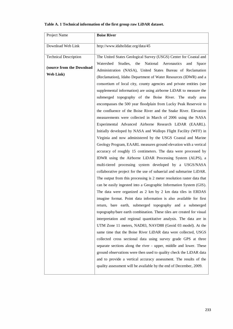
233
Table A. 1 Technical information of the first group raw LiDAR dataset.
Project Name Boise River
Download Web Link http://www.idaholidar.org/data/45
Technical Description
(source from the Download
Web Link)
The United States Geological Survey (USGS) Center for Coastal and
Watershed Studies, the National Aeronautics and Space
Administration (NASA), United States Bureau of Reclamation
(Reclamation), Idaho Department of Water Resources (IDWR) and a
consortium of local city, county agencies and private entities (see
supplemental information) are using airborne LiDAR to measure the
submerged topography of the Boise River. The study area
encompasses the 500 year floodplain from Lucky Peak Reservoir to
the confluence of the Boise River and the Snake River. Elevation
measurements were collected in March of 2006 using the NASA
Experimental Advanced Airborne Research LiDAR (EAARL).
Initially developed by NASA and Wallops Flight Facility (WFF) in
Virginia and now administered by the USGS Coastal and Marine
Geology Program, EAARL measures ground elevation with a vertical
accuracy of roughly 15 centimeters. The data were processed by
IDWR using the Airborne LiDAR Processing System (ALPS), a
multi-tiered processing system developed by a USGS/NASA
collaborative project for the use of subaerial and submarine LiDAR.
The output from this processing is 2 meter resolution raster data that
can be easily ingested into a Geographic Information System (GIS).
The data were organized as 2 km by 2 km data tiles in ERDAS
imagine format. Point data information is also available for first
return, bare earth, submerged topography and a submerged
topography/bare earth combination. These tiles are created for visual
interpretation and regional quantitative analysis. The data are in
UTM Zone 11 meters, NAD83, NAVD88 (Geoid 03 model). At the
same time that the Boise River LiDAR data were collected, USGS
collected cross sectional data using survey grade GPS at three
separate sections along the river - upper, middle and lower. These
ground observations were then used to quality check the LiDAR data
and to provide a vertical accuracy assessment. The results of the
quality assessment will be available by the end of December, 2009.
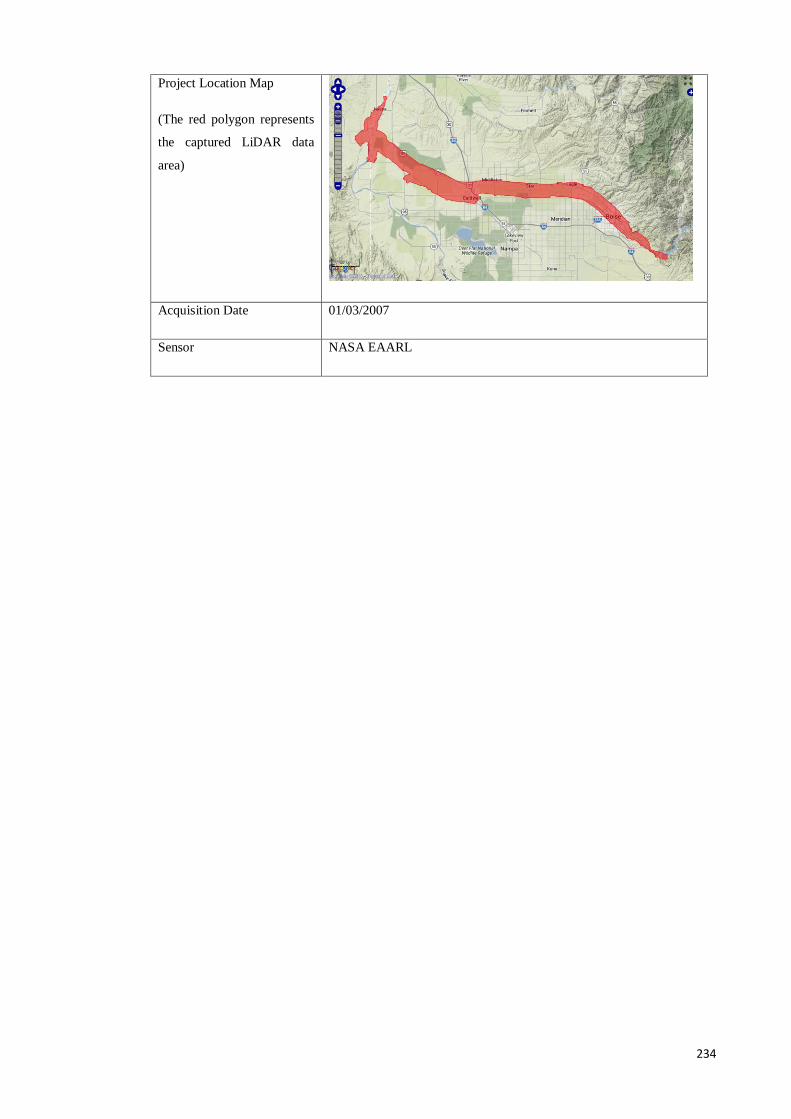
234
Project Location Map
(The red polygon represents
the captured LiDAR data
area)
Acquisition Date 01/03/2007
Sensor NASA EAARL
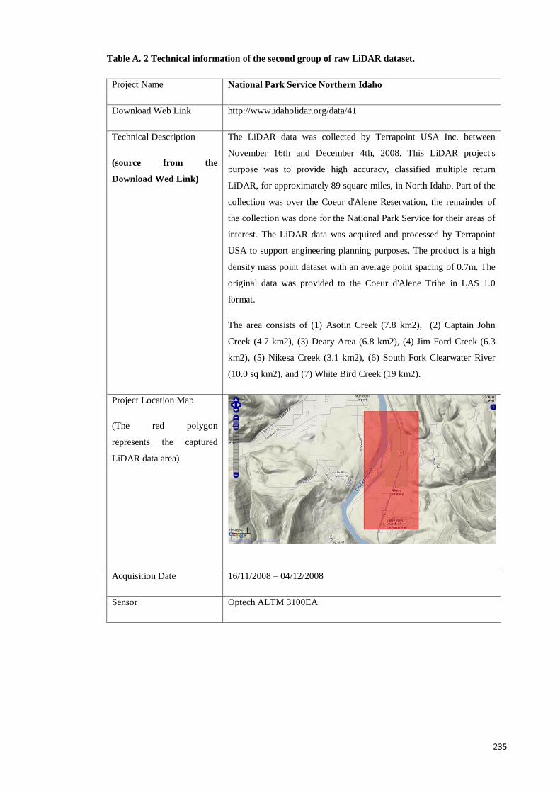
235
Table A. 2 Technical information of the second group of raw LiDAR dataset.
Project Name National Park Service Northern Idaho
Download Web Link http://www.idaholidar.org/data/41
Technical Description
(source from the
Download Wed Link)
The LiDAR data was collected by Terrapoint USA Inc. between
November 16th and December 4th, 2008. This LiDAR project's
purpose was to provide high accuracy, classified multiple return
LiDAR, for approximately 89 square miles, in North Idaho. Part of the
collection was over the Coeur d'Alene Reservation, the remainder of
the collection was done for the National Park Service for their areas of
interest. The LiDAR data was acquired and processed by Terrapoint
USA to support engineering planning purposes. The product is a high
density mass point dataset with an average point spacing of 0.7m. The
original data was provided to the Coeur d'Alene Tribe in LAS 1.0
format.
The area consists of (1) Asotin Creek (7.8 km2), (2) Captain John
Creek (4.7 km2), (3) Deary Area (6.8 km2), (4) Jim Ford Creek (6.3
km2), (5) Nikesa Creek (3.1 km2), (6) South Fork Clearwater River
(10.0 sq km2), and (7) White Bird Creek (19 km2).
Project Location Map
(The red polygon
represents the captured
LiDAR data area)
Acquisition Date 16/11/2008 – 04/12/2008
Sensor Optech ALTM 3100EA
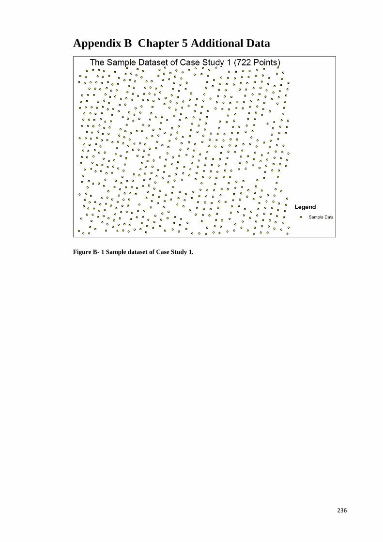
236
Appendix B Chapter 5 Additional Data
Figure B- 1 Sample dataset of Case Study 1.
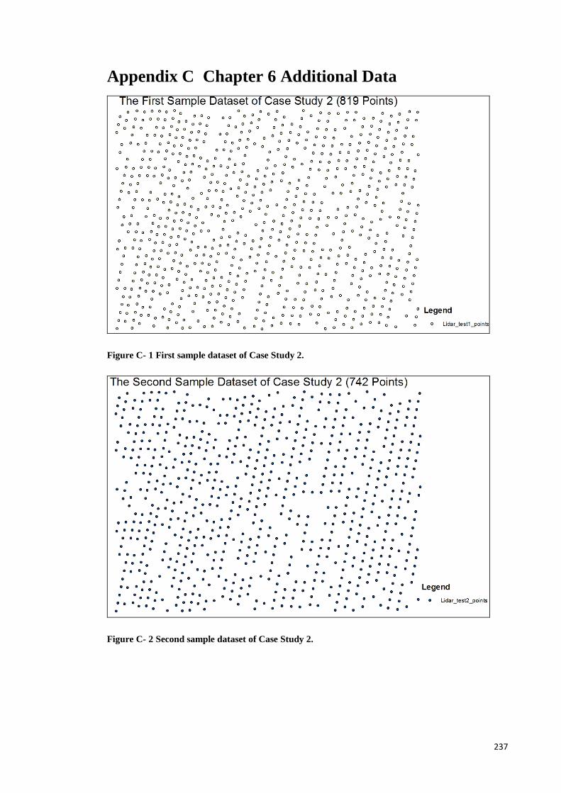
237
Appendix C Chapter 6 Additional Data
Figure C- 1 First sample dataset of Case Study 2.
Figure C- 2 Second sample dataset of Case Study 2.

238
Appendix D IDW Algrithem
The basic principle of IDW is that it assigns weights to neighboring observed values
based on distance and estimated grid values by averaging the values of sample data
points in the neighborhood of each processing grid (O’Sullivan and Unwin, 2003).
The standard IDW algorithm can be summarised as:
First the interpolated value, Zj, of a given point is estimated by:
(Equation 2.3)
In Equation 2.3, Wij is a weight between 0 and 1 which is based on the distance
from selected sample points to the estimated point, and Zi is the elevation of the
sample points. If distance is represented by Dij, the value of each weight value is
calculated by:
(Equation 2.4)
Where ( ) is the sum of all inverse distance weighted values and this
rule gives the proportional weight of each selected sample point. We can
determine that a large value of will give a small weight value, however, a
close distance between a sample point and the estimated point will lead to a
higher weight.
(Equation 2.5)
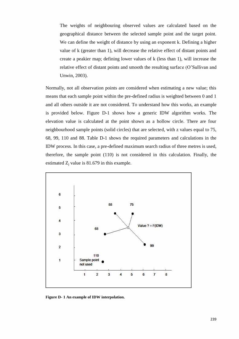
239
The weights of neighbouring observed values are calculated based on the
geographical distance between the selected sample point and the target point.
We can define the weight of distance by using an exponent k. Defining a higher
value of k (greater than 1), will decrease the relative effect of distant points and
create a peakier map; defining lower values of k (less than 1), will increase the
relative effect of distant points and smooth the resulting surface (O’Sullivan and
Unwin, 2003).
Normally, not all observation points are considered when estimating a new value; this
means that each sample point within the pre-defined radius is weighted between 0 and 1
and all others outside it are not considered. To understand how this works, an example
is provided below. Figure D-1 shows how a generic IDW algorithm works. The
elevation value is calculated at the point shown as a hollow circle. There are four
neighbourhood sample points (solid circles) that are selected, with z values equal to 75,
68, 99, 110 and 88. Table D-1 shows the required parameters and calculations in the
IDW process. In this case, a pre-defined maximum search radius of three metres is used,
therefore, the sample point (110) is not considered in this calculation. Finally, the
estimated Zj value is 81.679 in this example.
Figure D- 1 An example of IDW interpolation.
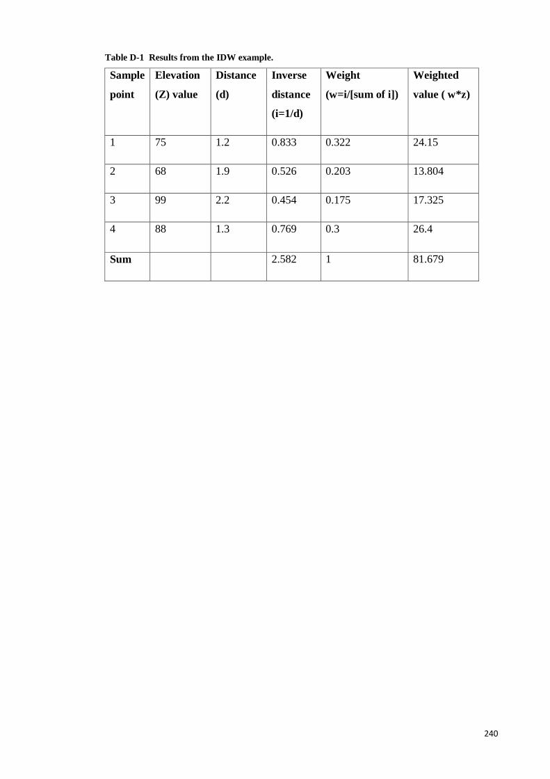
240
Table D-1 Results from the IDW example.
Sample
point
Elevation
(Z) value
Distance
(d)
Inverse
distance
(i=1/d)
Weight
(w=i/[sum of i])
Weighted
value ( w*z)
1 75 1.2 0.833 0.322 24.15
2 68 1.9 0.526 0.203 13.804
3 99 2.2 0.454 0.175 17.325
4 88 1.3 0.769 0.3 26.4
Sum 2.582 1 81.679
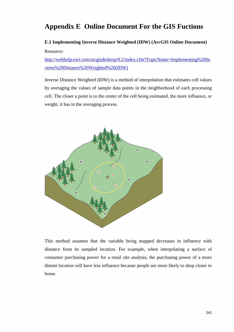
241
Appendix E Online Document For the GIS Fuctions
E.1 Implementing Inverse Distance Weighted (IDW) (ArcGIS Online Document)
Resource:
http://webhelp.esri.com/arcgisdesktop/9.2/index.cfm?TopicName=Implementing%20In
verse%20Distance%20Weighted%20(IDW)
Inverse Distance Weighted (IDW) is a method of interpolation that estimates cell values
by averaging the values of sample data points in the neighborhood of each processing
cell. The closer a point is to the center of the cell being estimated, the more influence, or
weight, it has in the averaging process.
This method assumes that the variable being mapped decreases in influence with
distance from its sampled location. For example, when interpolating a surface of
consumer purchasing power for a retail site analysis, the purchasing power of a more
distant location will have less influence because people are more likely to shop closer to
home.
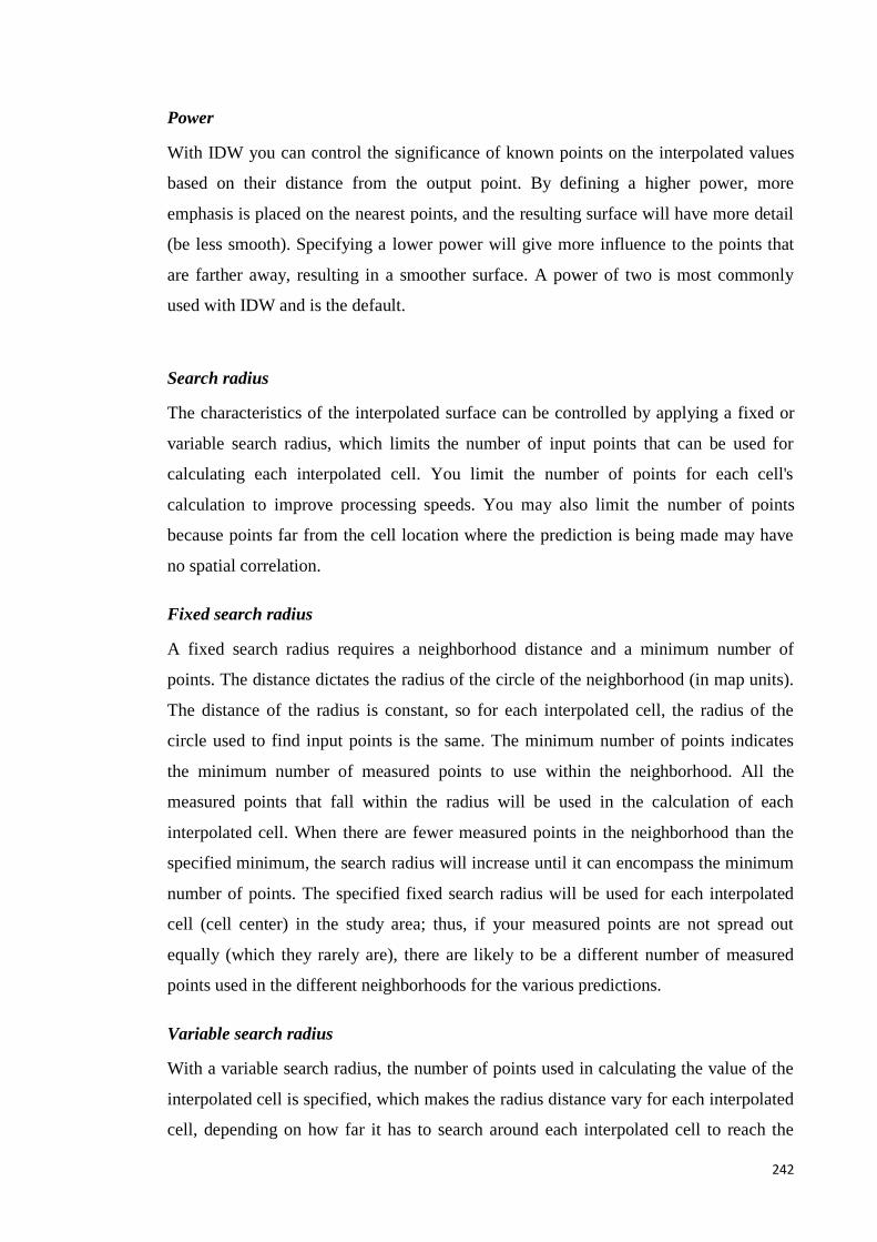
242
Power
With IDW you can control the significance of known points on the interpolated values
based on their distance from the output point. By defining a higher power, more
emphasis is placed on the nearest points, and the resulting surface will have more detail
(be less smooth). Specifying a lower power will give more influence to the points that
are farther away, resulting in a smoother surface. A power of two is most commonly
used with IDW and is the default.
Search radius
The characteristics of the interpolated surface can be controlled by applying a fixed or
variable search radius, which limits the number of input points that can be used for
calculating each interpolated cell. You limit the number of points for each cell's
calculation to improve processing speeds. You may also limit the number of points
because points far from the cell location where the prediction is being made may have
no spatial correlation.
Fixed search radius
A fixed search radius requires a neighborhood distance and a minimum number of
points. The distance dictates the radius of the circle of the neighborhood (in map units).
The distance of the radius is constant, so for each interpolated cell, the radius of the
circle used to find input points is the same. The minimum number of points indicates
the minimum number of measured points to use within the neighborhood. All the
measured points that fall within the radius will be used in the calculation of each
interpolated cell. When there are fewer measured points in the neighborhood than the
specified minimum, the search radius will increase until it can encompass the minimum
number of points. The specified fixed search radius will be used for each interpolated
cell (cell center) in the study area; thus, if your measured points are not spread out
equally (which they rarely are), there are likely to be a different number of measured
points used in the different neighborhoods for the various predictions.
Variable search radius
With a variable search radius, the number of points used in calculating the value of the
interpolated cell is specified, which makes the radius distance vary for each interpolated
cell, depending on how far it has to search around each interpolated cell to reach the
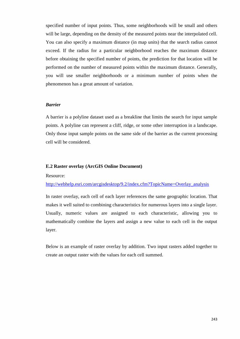
243
specified number of input points. Thus, some neighborhoods will be small and others
will be large, depending on the density of the measured points near the interpolated cell.
You can also specify a maximum distance (in map units) that the search radius cannot
exceed. If the radius for a particular neighborhood reaches the maximum distance
before obtaining the specified number of points, the prediction for that location will be
performed on the number of measured points within the maximum distance. Generally,
you will use smaller neighborhoods or a minimum number of points when the
phenomenon has a great amount of variation.
Barrier
A barrier is a polyline dataset used as a breakline that limits the search for input sample
points. A polyline can represent a cliff, ridge, or some other interruption in a landscape.
Only those input sample points on the same side of the barrier as the current processing
cell will be considered.
E.2 Raster overlay (ArcGIS Online Document)
Resource:
http://webhelp.esri.com/arcgisdesktop/9.2/index.cfm?TopicName=Overlay_analysis
In raster overlay, each cell of each layer references the same geographic location. That
makes it well suited to combining characteristics for numerous layers into a single layer.
Usually, numeric values are assigned to each characteristic, allowing you to
mathematically combine the layers and assign a new value to each cell in the output
layer.
Below is an example of raster overlay by addition. Two input rasters added together to
create an output raster with the values for each cell summed.
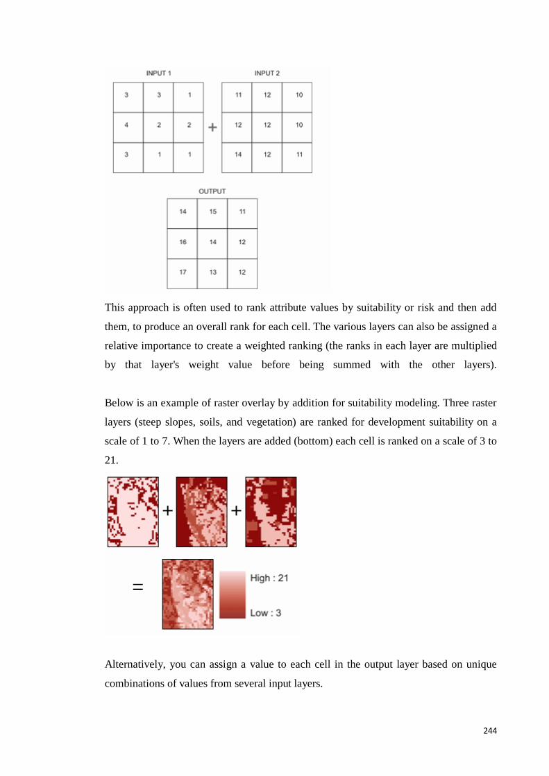
244
This approach is often used to rank attribute values by suitability or risk and then add
them, to produce an overall rank for each cell. The various layers can also be assigned a
relative importance to create a weighted ranking (the ranks in each layer are multiplied
by that layer's weight value before being summed with the other layers).
Below is an example of raster overlay by addition for suitability modeling. Three raster
layers (steep slopes, soils, and vegetation) are ranked for development suitability on a
scale of 1 to 7. When the layers are added (bottom) each cell is ranked on a scale of 3 to
21.
Alternatively, you can assign a value to each cell in the output layer based on unique
combinations of values from several input layers.
245
E.3 Calculating slope (ArcGIS Online Document)
Resource:
http://webhelp.esri.com/arcgisdesktop/9.2/index.cfm?TopicName=Calculating_slope
The Slope tool calculates the maximum rate of change between each cell and its
neighbors, for example, the steepest downhill descent for the cell (the maximum change
in elevation over the distance between the cell and its eight neighbors). Every cell in the
output raster has a slope value. The lower the slope value, the flatter the terrain; the
higher the slope value, the steeper the terrain. The output slope raster can be calculated
as percent of slope or degree of slope.
When the slope angle equals 45 degrees, the rise is equal to the run. Expressed as a
percentage, the slope of this angle is 100 percent. As the slope approaches vertical (90
degrees), the percentage slope approaches infinity.
The Slope tool is most frequently run on an elevation dataset, as the following diagrams
show. Steeper slopes are shaded red on the output slope raster. However, the function
can also be used with other types of continuous data, such as population, to identify
sharp changes in value.
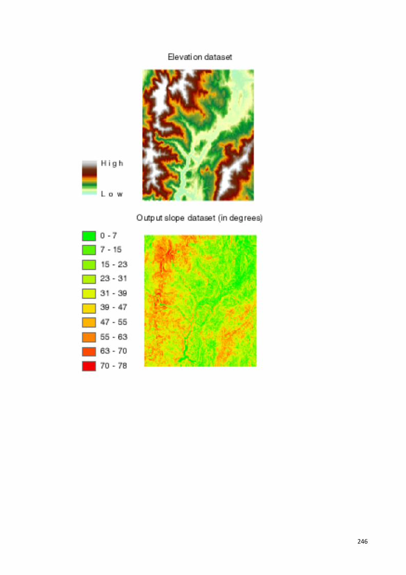
246
247
E.4 Selection (Understanding reclassification) (ArcGIS Online Document)
Resource:
http://webhelp.esri.com/arcgisdesktop/9.2/index.cfm?TopicName=Understanding_recla
ssification
The reclassification functions reclassify or change cell values to alternative values using
a variety of methods. You can reclass one value at a time or groups of values at once
using alternative fields; based on a criteria, such as specified intervals (for example,
group the values into 10 intervals); or by area (for example, group the values into 10
groups containing the same number of cells). The functions are designed to allow you to
easily change many values on an input raster to desired, specified, or alternative values.
All reclassification methods are applied to each cell within a zone. That is, when
applying an alternative value to an existing value, all the reclassification methods apply
the alternative value to each cell of the original zone. No reclassification method applies
alternative values to only a portion of an input zone.
Some of the many reasons to reclassify are detailed below.
Replacing values based on new information
Reclassification is useful when you want to replace the values in the input raster with
new values. This could be due to finding out that the value of a cell should actually be a
different value, for example, the land use in an area changed over time.
Grouping values together
You may want to simplify the information in a raster. For instance, you may want to
group together various types of forest into one forest class.
Reclassifying values of a set of rasters to a common scale
Another reason to reclassify is to assign values of preference sensitivity, priority, or
some similar criteria to a raster. This may be done on a single raster (a raster of soil type
may be assigned values of 1 to 10 to represent erosion potential) or with several rasters
to create a common scale of values.
For example, a soil type may be good to build on when soils are being viewed as an
input to a building suitability model. But for erosion, animal habitat, siting a pond, or
248
identifying farm land, that same soil type will have a different suitability weighting
based on the problem at hand. To represent a raster relative to these many different
suitability weightings, the values on the raster must be changed from nominal values—
values that represent a class—to interval or ratio values so that the values can be used in
relation to one another. It does not make sense to add soil type and land use to obtain a
building suitability raster. But if soil type and land use were in a measurement system
that represented a relative weighting to building suitability, analysis could be completed
freely between the rasters.
When identifying slopes most at risk of avalanche activity, input rasters might be slope,
soil type, and vegetation. Each of these rasters might be reclassified on a scale of 1 to 10
depending on the susceptibility of each attribute in each raster to avalanche activity—
that is, steep slopes in the slope raster might be given a value of 10 because they are
most susceptible to avalanche activity.
Each of the above examples is considered a suitability model. There are usually four
steps in producing a suitability map:
1. Input datasets. Decide which datasets you need as inputs.
2. Derive datasets. When applicable, create the datasets that you can derive from
your base input datasets— for example, slope and aspect can be derived from the
elevation raster. Create data from existing data to gain new information.
3. ssify datasets. Reclassify each dataset to a common scale (for example, 1 to 10),
giving higher values to more suitable attributes.
4. Weight and combine datasets. Weight datasets that should have more influence
in the suitability model if necessary, then combine them to find the suitable
locations.
Below is a flow diagram of a sample for finding the best locations for a school. The
input base layers are landuse, elevation, recreation sites, and existing schools. The
derived datasets are slope, distance to recreation sites, and distance to existing schools.
Each raster is then reclassified on a scale of 1 to 10. The reclassified rasters are added
together with distance from recreation sites and other schools having a higher weight.
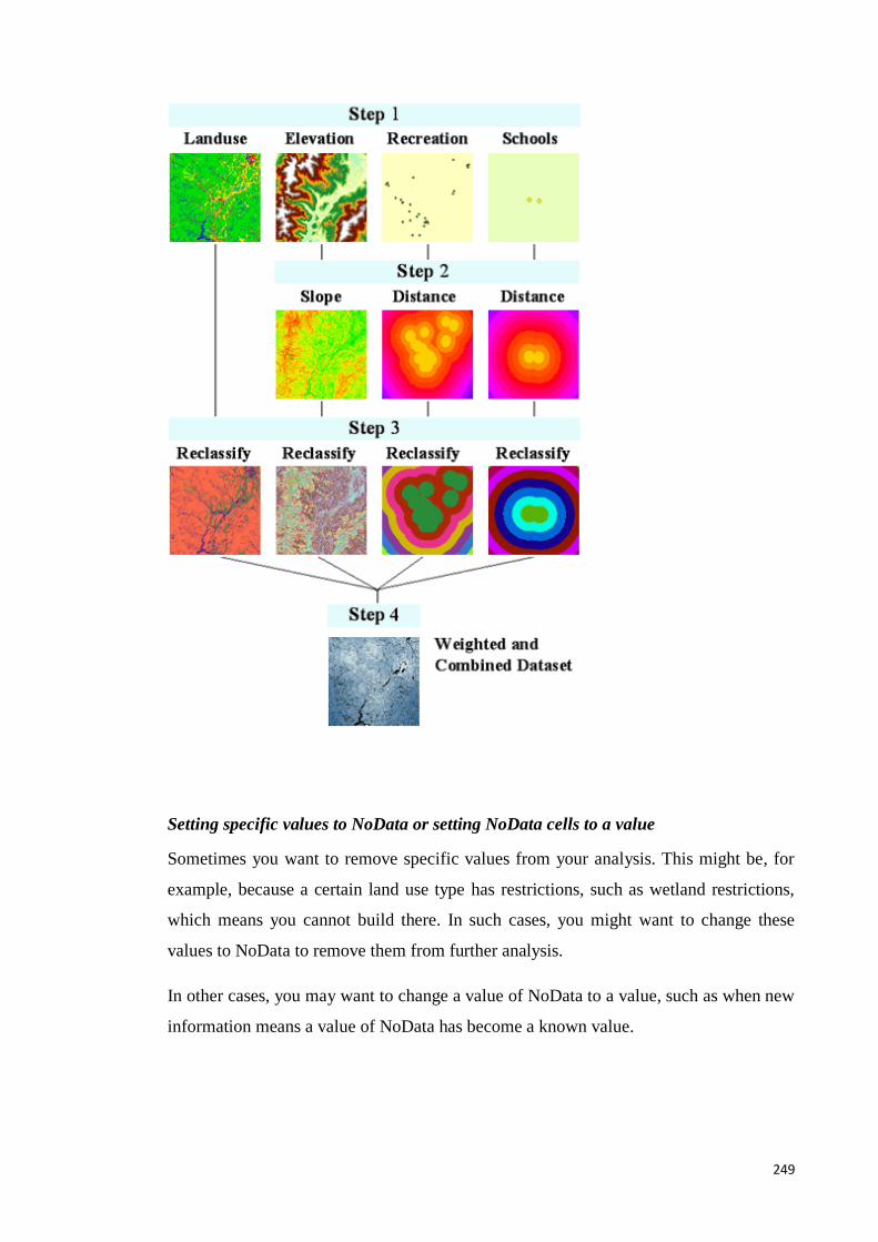
249
Setting specific values to NoData or setting NoData cells to a value
Sometimes you want to remove specific values from your analysis. This might be, for
example, because a certain land use type has restrictions, such as wetland restrictions,
which means you cannot build there. In such cases, you might want to change these
values to NoData to remove them from further analysis.
In other cases, you may want to change a value of NoData to a value, such as when new
information means a value of NoData has become a known value.

250
E.5 Distance (Understanding Euclidean distance analysis) (ArcGIS Online
Document)
Resource:
http://webhelp.esri.com/arcgisdesktop/9.2/index.cfm?TopicName=Understanding_Eucli
dean_distance_analysis
The Euclidean distance functions describe each cell's relationship to a source or a set of
sources.
There are three Euclidean functions:
1. Euclidean Distance gives the distance from each cell in the raster to the closest
source. Example of usage: What is the distance to the closest town?
2. Euclidean Allocation identifies the cells that are to be allocated to a source based
on closest proximity. Example of usage: What is the closest town?
3. Euclidean Direction gives the direction from each cell to the closest source.
Example of usage: What is the direction to the closest town?
The input raster used in each of the Euclidean functions and a discussion about the
output from the functions is described below.
The source
The source identifies the location of the objects of interest, such as wells, shopping
malls, roads, and forest stands. If the source is a raster, it must contain only the values
of the source cells while other cells must be NoData. If the source is a feature, it will
internally be transformed into a raster when you run the function.
The Euclidean distance output raster
The Euclidean distance output raster contains the measured distance from every cell to
the nearest source. The distances are measured as the crow flies (Euclidean distance) in
the projection units of the raster, such as feet or meters and are computed from cell
center to cell center.
The Euclidean Distance function is used frequently as a standalone function for
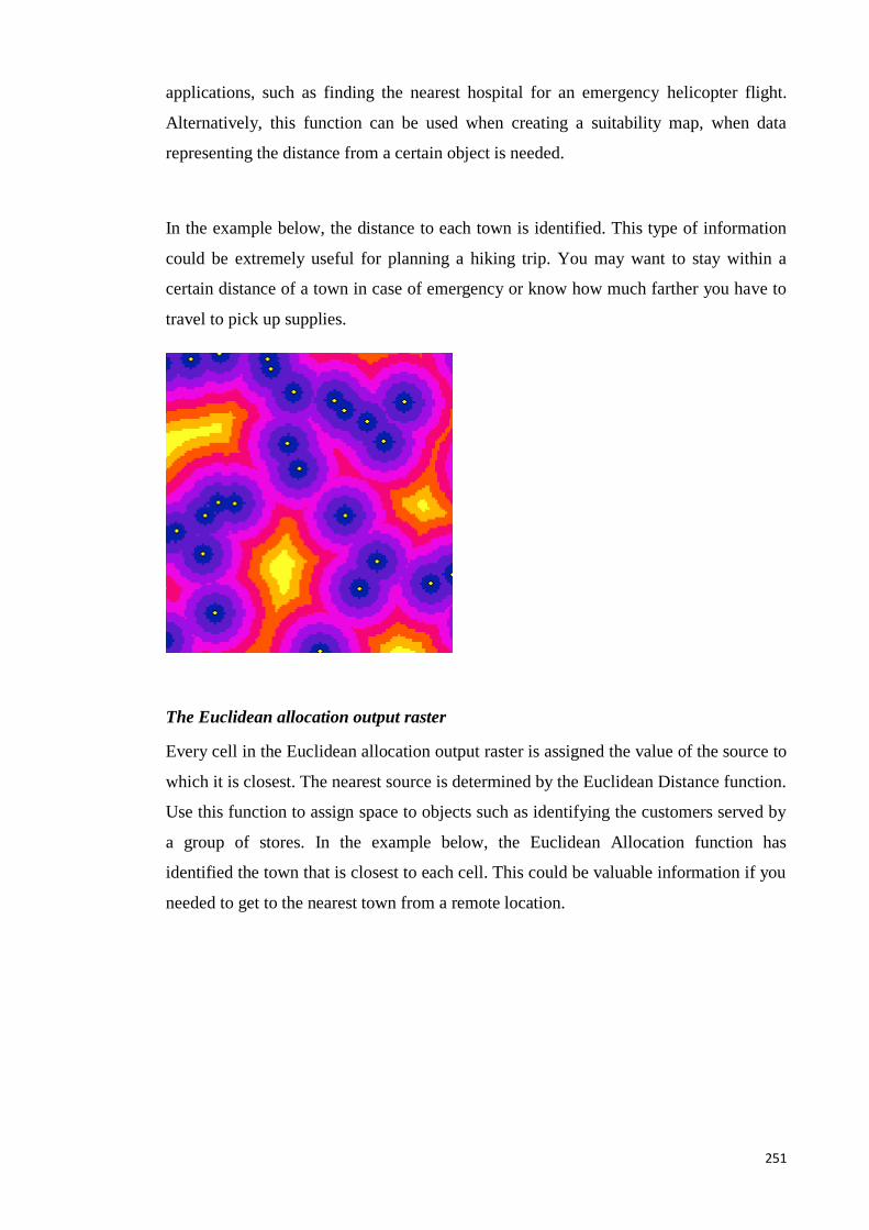
251
applications, such as finding the nearest hospital for an emergency helicopter flight.
Alternatively, this function can be used when creating a suitability map, when data
representing the distance from a certain object is needed.
In the example below, the distance to each town is identified. This type of information
could be extremely useful for planning a hiking trip. You may want to stay within a
certain distance of a town in case of emergency or know how much farther you have to
travel to pick up supplies.
The Euclidean allocation output raster
Every cell in the Euclidean allocation output raster is assigned the value of the source to
which it is closest. The nearest source is determined by the Euclidean Distance function.
Use this function to assign space to objects such as identifying the customers served by
a group of stores. In the example below, the Euclidean Allocation function has
identified the town that is closest to each cell. This could be valuable information if you
needed to get to the nearest town from a remote location.
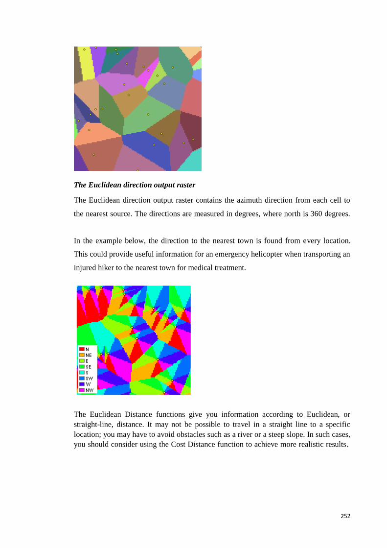
252
The Euclidean direction output raster
The Euclidean direction output raster contains the azimuth direction from each cell to
the nearest source. The directions are measured in degrees, where north is 360 degrees.
In the example below, the direction to the nearest town is found from every location.
This could provide useful information for an emergency helicopter when transporting an
injured hiker to the nearest town for medical treatment.
The Euclidean Distance functions give you information according to Euclidean, or
straight-line, distance. It may not be possible to travel in a straight line to a specific
location; you may have to avoid obstacles such as a river or a steep slope. In such cases,
you should consider using the Cost Distance function to achieve more realistic results.

253