Improving Solar and Load Forecasts by Reducing Operational ...

L

Energy Research and Development Division

FINAL PROJECT REPORT


FINAL PROJECT REPORT

Improving Solar and Load Forecasts by Reducing Operational Uncertainty

California Energy Commission

Gavin Newsom, Governor


Edmund G. Brown Jr., Governor

March 2019 | CEC-500-2019-023

Month Year | CEC-XXX-XXXX-XXX

PREPARED BY:

Primary Author(s):

Dr. Frank A. Monforte, Itron, Inc. Christine Fordham, Itron, Inc.

Jennifer Blanco, Itron, Inc. David Hanna, Itron, Inc.

Suraj Peri, Itron, Inc. Stephan Barsun, Itron, Inc.

Adam Kankiewicz, Clean Power Ben Norris, Clean Power

Itron, Inc. dba in California as IBS

12348 High Bluff Drive, Suite 210

San Diego, CA 92130

Phone: 858-724-2620 | Fax: 858-724-2690

http://www.itron.com/na/services/energy-and-water-consulting

Contract Number: EPC-14-001

PREPARED FOR:


Silvia Palma-Rojas

Project Manager

Alecia Gutierrez

Office Manager


Laurie ten Hope

Deputy Director


Drew Bohan

Executive Director

DISCLAIMER

This report was prepared as the result of work sponsored by the California Energy Commission. It does not

necessarily represent the views of the Energy Commission, its employees or the State of California. The Energy

Commission, the State of California, its employees, contractors and subcontractors make no warranty, express or

implied, and assume no legal liability for the information in this report; nor does any party represent that the uses

of this information will not infringe upon privately owned rights. This report has not been approved or

disapproved by the California Energy Commission nor has the California Energy Commission passed upon the

accuracy or adequacy of the information in this report.

i

ACKNOWLEDGEMENTS

The project team thanks Jim Blatchford, Gary Klein, Amber Motley, and Rebecca Webb, forecasting

staff at the California Independent System Operator, for their invaluable contribution to this

effort.

ii

PREFACE

The California Energy Commission’s Energy Research and Development Division supports

energy research and development programs to spur innovation in energy efficiency, renewable

energy and advanced clean generation, energy-related environmental protection, energy

transmission and distribution and transportation.

The California Public Utilities Commission established the Electric Program Investment Charge

(EPIC) in 2012 to fund public investments in research to create and advance new energy

solution, foster regional innovation and bring ideas from the lab to the marketplace. The

California Energy Commission and the state’s three largest investor-owned utilities – Pacific Gas

and Electric Company, San Diego Gas and Electric Company and Southern California Edison

Company –administered the EPIC funds and advance novel technologies, tools and strategies

that provide benefits to their electric ratepayers.

The Energy Commission is committed to ensuring public participation in its research and

development programs which promote greater reliability, lower costs and increase safety for

the California electric ratepayer and include:

• Providing societal benefits.

• Reducing greenhouse gas emission in the electricity sector at the lowest possible cost.

• Supporting California’s loading order to meet energy needs first with energy efficiency

and demand response, next with renewable energy (distributed generation and utility

scale), and finally with clean conventional electricity supply.

• Supporting low-emission vehicles and transportation.

• Providing economic development.

• Using ratepayer funds efficiently.

Improving Solar and Load Forecasts by Reducing Operational Uncertainty is the final report for

the grant number CEC-EPC-14-001 conducted by Itron, Inc. dba in California as IBS. The

information from this project contributes to Energy Research and Development Division’s EPIC

Program.

For more information about the Energy Research and Development Division, please visit the

Energy Commission’s website at www.energy.ca.gov/research/ or contact the Energy

Commission at 916-327-1551.

iii

ABSTRACT

Homeowners and businesses in California have installed numerous solar photovoltaic (PV)

systems because of California’s Renewable Portfolio Standard requirements as well as the

decreasing costs of PV. The California Independent System Operator (California ISO), who

operates California’s electric grid, does not measure behind-the-meter PV generation. The

California ISO and the electric utilities are facing the uncertainty associated with PV generation

profiles. The California ISO is conservatively forecasting and scheduling excess regulation and

spinning reserves because of this PV uncertainty. They must extend their load forecast models

to better predict when customers rely on the grid to meet their electricity requirements versus

relying on their behind-the-meter PV generation.

This project addresses this issue by advancing the state of the art in solar energy forecasting as

it relates to the operation of the California electric grid. It undertook four specific technical

tasks:

1) Investigate supplementing the California ISO’s current real-time solar data feeds.

2) Improve the California ISO’s solar production forecasts.

3) Investigate alternative net load forecasting methods to improve integrating PV

generation forecasts with an operational net load forecast, and

4) Estimate the monetary value of the alternative net load forecasts and develop a

framework for optimizing their use.

This research identified improvements necessary for real-time solar data and forecasts, and

alternative methods of net load forecasting that provide value to the grid and its stakeholders.

The research team also identified additional areas of future research.

The California ISO has adopted the findings of this research and implemented these methods,

providing savings for ratepayers and other stakeholders. In addition, the Australia Energy

Market Operator, the New York Independent System Operator, and the Independent Electricity

System Operator in Ontario Canada have implemented variations of these findings.

Keywords: Solar photovoltaics (PV), load forecasting, solar forecasting, forecast valuation

Please use the following citation for this report:

Monforte, Frank A.; Christine Fordham; Jennifer Blanco; David Hanna; Suraj Peri; Stephan

Barsun (Itron, Inc.); Adam Kankiewicz; and Ben Norris (Clean Power Research). 2019.

Improving Solar & Load Forecasts by Reducing Operational Uncertainty. California

Energy Commission. Publication number: CEC-500-2019-023

v

TABLE OF CONTENTS

Page

ACKNOWLEDGEMENTS ....................................................................................................................... i

PREFACE ................................................................................................................................................... ii

ABSTRACT .............................................................................................................................................. iii

TABLE OF CONTENTS ........................................................................................................................... v

LIST OF FIGURES ................................................................................................................................ viii

LIST OF TABLES ...................................................................................................................................... x

EXECUTIVE SUMMARY ........................................................................................................................ 1

Introduction ................................................................................................................................................ 1

Project Purpose .......................................................................................................................................... 1

Project Process ........................................................................................................................................... 1

Project Results ........................................................................................................................................... 4

Knowledge Transfer .................................................................................................................................. 5

Benefits to California ................................................................................................................................ 6

Chapter 1 Introduction ............................................................................................................................. 7

Technical Approach ...................................................................................................................................... 8

Chapter 2: Data Forecasting Accuracy Improvement ......................................................................... 9

Introduction and Background .................................................................................................................... 9

SolarAnywhere FleetView Forecasting Model ................................................................................... 10

Use of Data in Forecasts ........................................................................................................................... 14

Ground Irradiance Measurements ...................................................................................................... 14

Plant Availability .................................................................................................................................... 14

Concentrating Solar Power Resources ............................................................................................... 14

California Independent System Operator Real-time Data Feed ....................................................... 15

Description .............................................................................................................................................. 15

Data Application Programming Interface and Structure Formats ............................................... 16

Chapter 3: Grid-Connected and Embedded Photovoltaic Fleet Forecasting Accuracy .............. 17

Introduction and Background ................................................................................................................. 17

Project Partnerships .................................................................................................................................. 17

vi

Enhancements Using Embedded System Production Data ............................................................... 18

Module Degradation .............................................................................................................................. 18

Soiling ....................................................................................................................................................... 20

System Availability ................................................................................................................................. 22

Improving System Specifications by Inference ................................................................................ 23

Other Forecast Improvements ............................................................................................................. 27

Inverter Power Curve ............................................................................................................................. 27

Ensemble Methods ................................................................................................................................. 28

Representative Photovoltaic System Fleets ...................................................................................... 28

Dynamic Regional Fleet Capacity Updates ....................................................................................... 37

Historical Behind-the-meter Photovoltaic Fleet Production Modeling ........................................ 39

Robustness of the California Independent System Operator Forecast Delivery ...................... 40

Real-time Data Feedback ...................................................................................................................... 40

Chapter 4: Improving Short-term Load Forecasts by Incorporating Solar Photovoltaic

Generation ................................................................................................................................................ 42

Background .................................................................................................................................................. 42

California Independent System Operator Short-Term Load Forecast Model ............................ 42

The Impact of Solar Photovoltaic on the California Independent System Operator Short-

Term Load Forecast ............................................................................................................................... 44

Incorporating the Impact of Solar Photovoltaic Generation in a Load Forecast .......................... 44

Error Correction ...................................................................................................................................... 45

Reconstituted Loads .............................................................................................................................. 46

Model Direct ............................................................................................................................................ 46

Solar Photovoltaic Generation Estimates .............................................................................................. 46

Clean Power Research Solar Generation Estimates ......................................................................... 46

Cloud Cover Driven Solar Generation Estimates ............................................................................. 48

Forecast Simulations ................................................................................................................................. 54

Forecast Performance Measurements ................................................................................................ 55

Simulation Results Summary................................................................................................................... 56

California Independent System Operator Total Simulation Results ........................................... 57

Pacific Gas & Electric Bay Area Simulation Results ......................................................................... 62

Pacific Gas & Electric Non Bay Area Simulation Results ................................................................ 65

Southern California Edison Coastal Simulation Results ................................................................ 68

Southern California Edison Inland Simulation Results .................................................................. 71

San Diego Gas & Electric Total Simulation Results ......................................................................... 74

vii

Statistical Estimates of Solar Photovoltaic Load Impacts ................................................................. 77

Chapter 5: Forecasting Valuation and Framework Analysis .......................................................... 82

Introduction and Background ................................................................................................................. 82

Valuation of Alternative Forecast Method ............................................................................................ 82

Valuation Methodology ......................................................................................................................... 83

Locational Marginal Prices .................................................................................................................... 84

Hour Ahead Locational Marginal Prices ............................................................................................ 86

Ancillary Services Prices ....................................................................................................................... 87

Valuation Results Summary ..................................................................................................................... 90

Costing Period Components ................................................................................................................ 91

Forecasting Framework Overview .......................................................................................................... 93

Examination of External Factors and Value ...................................................................................... 93

Forecasting Framework Analysis ............................................................................................................ 97

Algorithmic Framework Exploration .................................................................................................. 97

Framework Analysis Summary ................................................................................................................ 98

Summary of Results ............................................................................................................................... 98

Chapter 6: Conclusions and Recommendations .............................................................................. 100

Data Forecasting Accuracy Improvement ........................................................................................... 100

Conclusions ........................................................................................................................................... 100

Recommendations ................................................................................................................................ 100

Grid-Connected and Embedded Photovoltaic Fleet Forecasting Accuracy .................................. 100

Conclusions ........................................................................................................................................... 100


Improving Short-Term Load Forecasts by Incorporating Solar Photovoltaic Generation ........ 100

Conclusions ........................................................................................................................................... 100


Forecast Valuation & Framework Analysis ......................................................................................... 102

Conclusions ........................................................................................................................................... 102


GLOSSARY AND ACRONYMS ........................................................................................................ 104

REFERENCES ........................................................................................................................................ 106

viii

LIST OF FIGURES

Page

Figure 1: California Statewide Behind-The-Meter Solar Generation Capacity ............................ 7

Figure 2: Mapping of All ~78,000 Behind-the-meter Photovoltaic Systems in the

California Independent System Operator .......................................................................................... 11

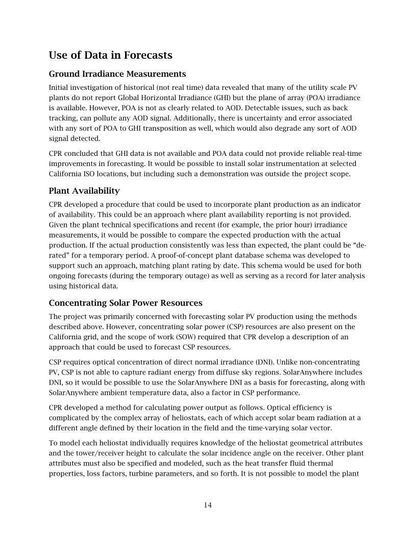
Figure 3: Relationship Between Average Mean Absolute Error for 207 Sites Selected

from the Itron Data that Both have Five Years of Data and Annual Mean Absolute

Error less than 20 percent ....................................................................................................................... 19

Figure 4: Degradation via Monthly Max Values ............................................................................... 20

Figure 5: Soiling by Year ........................................................................................................................ 21

Figure 6: Histogram of System Availability ...................................................................................... 22

Figure 7: Availability as a Function of System Size ......................................................................... 23

Figure 8: Measured Photovoltaic Output, Example One ................................................................. 24

Figure 9: Measured Photovoltaic Output, Example Two ................................................................. 25

Figure 10: Measured and Simulated Photovoltaic Output for Selected Days, Example

One ............................................................................................................................................................. 25

Figure 11: AC Capacity Underestimated, Example Two .................................................................. 26

Figure 12: DC to AC Ratio Overestimated, Example Two ............................................................... 26

Figure 13: Actual Inverter Power Curve versus Existing Default .................................................. 28

Figure 14: Cumulative Installed Behind-the meter Systems in California .................................. 29

Figure 15: Representative Fleet with System Locations at 0.4° Latitude/Longitude

Spacing ...................................................................................................................................................... 32

Figure 16: Relative Mean Absolute Error for Representative Fleets ............................................. 34

Figure 17: Thirty-Minute Power Value Correlation ......................................................................... 35

Figure 18: California Behind-the meter Fleet Capacity 2008 to 2016 ............................................. 38

Figure 19: Southern California Edison Coastal Photovoltaic Production .................................... 40

Figure 20: Ratio of Solar Generation Volatility to Load Volatility (Pacific Gas &

Electric Total) ........................................................................................................................................... 48

Figure 21: Ratio of Solar Generation Volatility to Load Volatility: Southern California

Edison Total ............................................................................................................................................. 49

ix

Figure 22: Ratio of Solar Generation Volatility to Load Volatility: San Diego Gas &

Electric ....................................................................................................................................................... 49

Figure 23: Ratio of Solar Generation Volatility to Load Volatility: Investor-owned

Utility Comparison ................................................................................................................................. 50

Figure 24: CPR versus Cloud Cover Solar Generation (MWh): Pacific Gas & Electric

Bay Area .................................................................................................................................................... 52

Figure 25: CPR versus Cloud Cover Solar Generation (MWh): Pacific Gas & Electric

Non Bay Area ........................................................................................................................................... 52

Figure 26: CPR versus Cloud Cover Solar Generation (MWh): Southern California

Edison Coastal ......................................................................................................................................... 53

Figure 27: CPR versus Cloud Cover Solar Generation (MWh): Southern California

Edison Inland ........................................................................................................................................... 53

Figure 28: CPR versus Cloud Cover Solar Generation (MWh): San Diego Gas &

Electric ....................................................................................................................................................... 54

Figure 29: California Independent System Operator Total, All Seasons, All Cloud

Cover Conditions .................................................................................................................................... 59

Figure 30: California Independent System Operator Total, All Seasons, Clear ......................... 60

Figure 31: Pacific Gas & Electric Bay Area, All Seasons, All Cloud Cover Conditions ............. 63

Figure 32: Pacific Gas & Electric Bay Area, All Seasons, Clear ...................................................... 64

Figure 33: Pacific Gas & Electric Non Bay Area, All Seasons, All Cloud Cover

Conditions ................................................................................................................................................ 66

Figure 34: Pacific Gas & Electric Non Bay Area, All Seasons, Clear ............................................. 67

Figure 35: Southern California Edison Coastal, All Seasons, All Cloud Cover

Conditions ................................................................................................................................................ 69

Figure 36: Southern California Edison Coastal, All Seasons, Clear .............................................. 70

Figure 37: Southern California Edison Inland, All Seasons, All Cloud Cover

Conditions ................................................................................................................................................ 72

Figure 38: Southern California Edison Inland, All Seasons, Clear ............................................... 73

Figure 39: San Diego Gas & Electric Total, All Seasons, All Cloud Cover Conditions ............. 75

Figure 40: San Diego Gas & Electric Total, All Seasons, Clear ...................................................... 76

Figure 41: Estimated Load Impact of Solar Photovoltaic Generation: California

Independent System Operator Total ................................................................................................... 78

x

Figure 42: Estimated Load Impact of Solar Photovoltaic Generation: Pacific Gas &

Electric Total ............................................................................................................................................ 79

Figure 43: Estimated Load Impact of Solar Photovoltaic Generation: Southern

California Edison Total .......................................................................................................................... 79

Figure 44: Estimated Load Impact of Solar Photovoltaic Generation: San Diego Gas &

Electric Total ............................................................................................................................................ 80

Figure 45: Weekday Hourly Locational Marginal Price Prices – Summer 2014 .......................... 85

Figure 46: Weekday Hourly Locational Marginal Price Prices – Spring 2015.............................. 85

Figure 47: Weekday Hourly Hour Ahead Scheduling Process Locational Marginal

Price – Summer 2014 ............................................................................................................................... 86

Figure 48: Weekday Hourly Hour Ahead Scheduling Process Locational Marginal

Price – Spring 2015 .................................................................................................................................. 87

Figure 49: Weekday Regulation Up Prices – Summer 2014 ............................................................ 88

Figure 50: Weekday Regulation Down Prices – Summer 2014 ...................................................... 88

Figure 51: Weekday Regulation Up Prices – Spring 2015 ............................................................... 89

Figure 52: Weekday Regulation Down Prices – Spring 2015 ......................................................... 89

Figure 53: Pacific Gas & Electric Bay Area – Alternative Forecasts Valuation vs. Prices,

Irradiance and Temperature.................................................................................................................. 94

Figure 54: Pacific Gas & Electric Bay Area – Alternative Forecasts Valuation vs. Prices,

Irradiance and Temperature.................................................................................................................. 95

Figure 55: Pacific Gas & Electric Bay Area – Low Alternative Forecasts Valuation vs.

Prices, Irradiance and Temperature ..................................................................................................... 96

Figure 56: Pacific Gas & Electric Bay Area – Alternative Forecasts Valuation vs.

Difference Between Day-of and Day-Ahead Forecasts ................................................................... 97

LIST OF TABLES

Page

Table 1: Soiling Analysis Results ........................................................................................................ 21

Table 2: Fleet Availability Statistics .................................................................................................... 22

Table 3: Summary of Results for Three Systems .............................................................................. 27

xi

Table 4: Number of Systems in Representative Fleets by Spatial Resolution and

Orientation Bin ........................................................................................................................................ 31

Table 5: Estimated Reduction in Simulation Times for Representative Fleets Relative

to Baseline Fleet ....................................................................................................................................... 36

Table 6: Fleet Scaling Factors and Ratings ........................................................................................ 39

Table 7: Monthly Valuation of Alternative Forecasts by California-ISO Zone .......................... 90

Table 8: Annual Valuation of Alternative Forecasts by California ISO Zone ............................ 91

Table 9: PG&E Bay Area Baseline Forecast Costing Period Components ................................... 91

Table 10: PG&E Bay Area Alternative Forecast Costing Period Components ............................ 92

Table 11: PG&E Bay Area Alternative Forecast Valuation by Period Component .................... 93

Table 12: Energy Cost Summary by Machine Learning Models .................................................... 99

1

EXECUTIVE SUMMARY

Introduction

Homeowners and businesses in California have installed numerous solar photovoltaic (PV)

systems because of Renewable Portfolio Standard requirements and the decreasing costs of PV.

The installed capacity of behind-the-meter solar in California is nearly 6 gigawatts, and

researchers expect this capacity to increase substantially by 2020. Behind-the-meter generation

supplies a portion of the electricity consumed by end-users (such as residential, commercial,

industrial, agriculture, and other customers).

The California Independent System Operator (California ISO) operates California’s electrical grid

but does not measure behind-the-meter PV generation. As a result, that generation is not

captured in the California ISO’s load forecast models, which only include factors that affect

gross end-user electricity consumption. With more behind-the-meter solar PV, these load

forecast models will need to better predict when end users will rely on the grid to meet their

electricity requirements versus relying on their solar generation. Additionally, the increasing

number of larger scale PV plants is exacerbating variable electricity from renewable resources

that the California ISO must then compensate for with conventional generating resources.

Uncertainty associated with PV generation profiles is the key challenge facing the California ISO

and electric utilities as they integrate higher concentrations of PV into the grid. PV is inherently

an intermittent, or irregular, resource, while utilities must maintain high system reliability at

low costs. The California ISO’s current scheduling of conventional generators like natural gas

plants to maintain system stability is conservative and reflects the uncertainty in PV.

Project Purpose

Itron, Inc. proposed advancing the state of the art in solar energy forecasting as it relates to

operating the California electric grid. Itron submitted its proposal under the Electric Program

Investment Charge (EPIC) funds, with Clean Power Research, LLC identified as a major

subcontractor.

While numerous efforts have attempted to improve predicting solar PV generation, they often

failed to address one of the core challenges facing grid operators—uncertainty in net load

forecasts. This project explored how to reduce the operational uncertainty in PV and net load

forecasts with high accuracy forecasts and linking them to net load forecasts at more precise

time intervals. Increased accuracy in estimating and incorporating PV into net load forecasts

will enable better integration of intermittent PV generation in California and provide substantial

savings in the associated wholesale energy market costs.

Project Process

Itron and Clean Power Research supplied the California ISO with solar forecasts and net load

forecasts separately. The research team coordinated with the California ISO in implementing

the approaches to their scheduling operations while developing the improved forecast methods.

The team used 15-minute to two-hour forecast horizons in five-minute time intervals to

2

evaluate the forecast performance improvements. In addition, the research team used a second

set of forecast performance metrics to quantify the reduction of net load forecast uncertainty.

The team used the error in the net load forecast to estimate how much excess generation

California needed to ensure adequate power was available. Finally, the team used wholesale

energy market cost analysis to further quantify savings from more accurate forecasts.

The research team used a series of four analyses to accomplish the research: data forecasting

accuracy improvement; grid-connected and embedded PV fleet forecasting accuracy; improving

short-term load forecasts by incorporating solar PV generation; and forecasting evaluation and

framework analysis.

Data Forecasting Accuracy Improvement

The project investigated using real-time data taken from utility-scale and behind-the-meter

resources to improve solar production forecasts. This data could potentially improve forecasts

by providing a "true up" for calculated solar irradiance (solar energy as radiation) as well as an

indication of individual power plant availability. The project sought a method for forecasting

production from concentrating solar power resources. Concentrating solar power resource

forecasting is more complicated than solar PV forecasting because output depends not only on

the solar intensity, but also on the position of the sun. Concentrating solar power concentrates

light, so it can only make use of direct “beam” irradiance, whereas non-concentrating PV uses

three types of solar radiation: beam, diffuse (refracted throughout the sky and received from

many directions) and reflected (such as from the ground).

Grid-Connected and Embedded Photovoltaic Fleet Forecasting Accuracy

The project analyzed potential methods for improving solar forecasts. Solar forecasting

includes forecasting for individual, utility-scale resources and aggregated behind-the-meter

"fleet" resources. Possible improvements to the solar forecasts include incorporating factors

such as: age-related degradation, improvements in inverter modeling, incorporating ever-

changing amounts of solar capacity, and handling real-world performance issues such as

soiling, system outages, and shading.

Improving Short-Term Load Forecasts by Incorporating Solar Photovoltaic Generation

The California ISO Baseline Load Forecast Model provided forecasts of measured loads for

forecast horizons of 15 minutes ahead to ten days ahead. The baseline modeling framework is

composed of a set of 193 individual forecast models. None of these models included the impact

of behind-the-meter solar PV on measured loads. The research team extended the existing

California ISO load forecast models to capture the influence of behind-the-meter solar PV and

predict an increasingly volatile load. This study evaluated three alternative model approaches

for extending the California ISO load forecast framework.

1. Error Correction. The Error Correction approach implemented what many system

operators did initially when faced with the problem of solar PV generation. They made

ex post adjustments of the load forecast to account for forecasted values of solar PV

generation.

3

2. Reconstituted Loads. Under the reconstituted loads approach, the research team

reconstituted the historical time series of measured load by adding back estimates of

solar PV generation. The team then re-estimated the load forecast model against the

reconstituted loads. The team then adjusted, ex post, the reconstituted load forecasts by

subtracting away forecasts of solar PV generation to form a forecast of measured loads.

3. Model Direct. Under this approach, the research team directly estimated the weight

placed on the solar PV generation data by including these data as an explanatory

variable in the load forecast models. The estimated coefficient on the solar PV

generation variable is the weight.

To evaluate the forecast performance of the alternative model approaches, the study simulated

a series of 24-hour ahead load forecasts. The research team compared the forecast errors to the

corresponding baseline model load forecast errors. The study relied on two sources of behind-

the-meter solar PV generation estimates—Clean Power Research’s solar generation estimates

and cloud-cover driven solar generation estimates.

Forecasting Valuation and Framework Analysis

The study considered how the monetary value associated with the alternative net load forecasts

would affect stakeholder long-term and short-term costs. The research team developed

alternative net load forecasts as short-term forecasts for the next-day and day-of wholesale

electricity markets within California. Determining the short-term avoided costs associated with

the alternative forecasts requires the use of short-term wholesale electricity prices and not

long-term avoided capital costs.

The research team computed the avoided costs (valuation) of electricity associated with using

the alternative forecasts over the California ISO’s baseline forecasting models by costing the

electricity from each forecast and then taking the difference. This difference in costs

determines the value of using the alternative forecasts. The team performed the evaluation for

each of the five zones (Pacific Gas and Electric (PG&E) Bay Area, PG&E Not Bay, Southern

California Edison (SCE) Inland, SCE Coastal, and San Diego Gas and Electric (SDG&E)) used in the

development of the alternative forecast methodology and at the total California ISO level (sum

of the five zones).

This study examined highly influential factors in determining the value associated with the

alternative net load forecasts. The team performed this examination as a precursor to

developing a framework for using the alternate forecasts.

The research team did not find any clearly observable correlations. The team used three

machine learning approaches to investigate the creation of a framework for optimizing the

choice of forecasting method. These included a number of different machine learning

techniques and approaches. The project team applied these algorithms to each of the five

California ISO zones (PG&E Bay Area, PG&E Not Bay, SCE Inland, SCE Coastal, and SDG&E).

4

Project Results


Using ground irradiance measurements from utility-scale resources was problematic because

plants do not report global horizontal irradiance (the amount of radiation received on a surface

horizontal to the ground), but irradiance measured on the tilted surface of the solar modules.

The project developed a method to estimate how often solar power plants were online when the

sun was shining. Finally, the project introduced an approach to forecasting concentrating solar

power resources, but also identified forecast difficulties with some aspects of this approach.


The project incorporated several forecast improvements. The project team introduced a

method for tracking system installation dates and added a correction for module degradation.

The project advanced methods for determining system specifications and shading based on

measured production inputs, rather than relying upon installer-supplied data which is not

always accurate. Forecast improvements also included the use of model-specific inverter power

curves; advanced ensemble methods leveraging forecasts from multiple sources. The project

team evaluated a method to increase forecast performance using representative fleets and

developed a process to automatically update FleetView™ (a software program developed by

Clean Power Research) to incorporate monthly utility-reported behind-the-meter capacity

increases. Sacramento Municipal Utility District (SMUD), SCE and PG&E held utility partner

meetings to quantify the impact of distributed PV on the distribution grid.


The team compared the baseline forecast to each of the six different forecasting methodologies:

California ISO as a whole, the three investor owned utilities, and the five California ISO zones

(PG&E Bay Area, PG&E Non-Bay Area, SCE Coastal, SCE Inland, and SDG&E). In general, the

results showed that:

• Not adjusting the California ISO baseline forecast models will only lead to further

erosion of forecast accuracy and a greater dispersion of forecast errors.

• Direct modelling performed better than the baseline and other methods in the near term

(fifteen minutes to four hours in advance). The Reconstituted Load Approach performed

better for longer time horizons from four hours through to day ahead horizons. That

suggests that a hybrid or ensemble approach that combines these two methods is

optimal.

• SDG&E showed better improvements from forecasts that integrated behind-the-meter PV

forecasts than the California ISO or any of the other California ISO zones. This could be

a result of a smaller geographic area combined with a higher penetration of behind-the-

meter PV.

• Hourly cloud cover driven estimates of solar generation can provide benefit over doing

nothing, however the detailed bottom-up approach implemented by Clean Power

Research yields superior results.

5

• The findings also indicated that 1 megawatt of solar PV generation may not reduce what

the California ISO measures as load by the same amount, 1 megawatt. A possible

explanation for this counterintuitive finding is that the California ISO only measures

what happens in front of the meter. Installing solar PV can result in fundamental

behind-the-meter behavioral changes in how consumers use end-use equipment, which

mutes the impact of solar PV generation on load.

• The model direct approach allows some investigation into how much of the solar PV

generation results in net load increases associated with this type of behavioral change.

Further research can determine the extent to which penetration of solar PV is leading to

behavioral changes.

Forecasting Valuation and Framework Process and Analysis

The research team developed a method for estimating the avoided costs, or value, associated

with the alternative forecasts. The team calculated the cost of acquiring electricity in the

California wholesale markets for each of the forecasting methodologies and compared the

alternative forecast to the existing baseline forecast. In general, the results show:

• In total, the alternative forecast method provides positive value at the California ISO

level across all years.

• At the California ISO level, the valuation varies significantly in magnitude across years.

• At the individual zonal level, the alternative forecast does not provide positive value in

all months or years.

• There does not appear to be a consistent pattern as to which months or zones will have

a positive valuation.

Machine learning is the field of computer science where computers learn from data without

being explicitly programmed. The project team developed and applied a framework to choose

the least costly forecast method, which uses several data mining and machine learning

algorithms. One of these machine learning algorithms did appear to improve results but was

deemed to be too complicated to be actionable for system operators.

The research team recommends more research into machine learning before deciding on a more

sophisticated framework.

Knowledge Transfer

The technology analyzed under this project is being used today by the California ISO to

improve net load forecasts. Other Independent System Operators that have adopted at least

some variation of the improved net load framework include New York ISO, ISO New England,

IESO (Ontario, Canada), AEMO (Australia) and Western Power (Australia).

In addition, multiple conference presentations and papers were completed to disseminate the

learnings form this analysis. The team also published an Energy Commission report on

improving short-term load forecasts by incorporating solar PV generation to share these first-

of-their-kind results with stakeholders and the international community interested in the

6

subject (available at https://www.energy.ca.gov/2017publications/CEC-500-2017-031/CEC-500-

2017-031.pdf.

Benefits to California

This research is important to stakeholders (California ISO, generation providers, utilities, and

ratepayers) because it shows that improvements in solar and net load forecasting methods can

provide positive financial impacts in the scheduling and procurement of electricity in the

wholesale electric market within California. The results of this research have shown that, just in

the period covered by this analysis, the potential savings to all stakeholders would have been

about $9 million. With further growth in solar and improvements in integrating behind the

meter solar into the California ISO net load forecasts, the team anticipates it can achieve even

greater cost reductions. The California ISO adopted the findings demonstrated in this research

and placed them in production. They are currently generating saving for ratepayers and other

stakeholders. In addition, AEMO, the New York ISO, and IESO in Ontario Canada have all

implemented in production variations of the models.

This research is also important to stakeholders because it sets the groundwork for further

research into developing a framework to optimize the use of the alternative forecast method by

the California ISO to develop its net load forecast. It may be possible to develop a framework

for choosing when to use the alternative forecast to optimize its value to all stakeholders.

In additional to financial savings, emission savings should result from the reduction in the need

for spinning reserves as part of this project. Finally, by reducing the need for resources to

balance intermittent renewables, this project should enable a higher proportion of solar

generation on California’s grid.

7

Chapter 1 Introduction

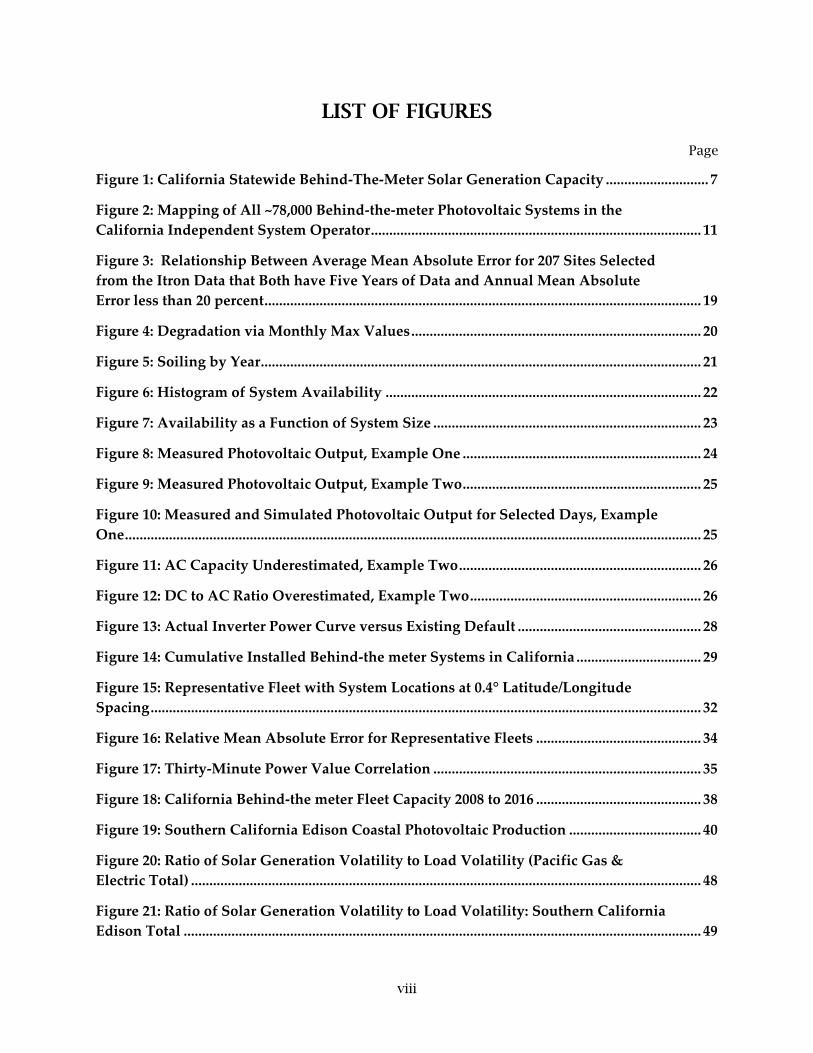
The key challenge facing the California Independent System Operator (California ISO) and the

electric utilities as they integrate higher and higher concentrations of photovoltaics (PV) into

the grid is the uncertainty associated with PV generation profiles. Figure 1 shows the growth of

behind-the-meter (BTM) PV in California. PV generation is inherently an intermittent resource

and utilities must maintain high system reliability at low costs. The California ISO’s current

scheduling of conventional generators and spinning reserves is conservative and reflects the

uncertainty in PV. To reduce the reliance on regulation services and spinning reserves, the

California ISO requires improved solar generation and measured load forecasts.

Itron, Inc., developed a proposal in June 2014 to the California Energy Commission (Energy

Commission) to address this issue by advancing the state of the art in solar energy forecasting

as it relates to the operation of the California electric grid. The Itron team submitted its

proposal under the Electric Program Investment Charge (EPIC) funds, with Clean Power

Research, LLC (CPR) identified as a major subcontractor. The Energy Commission awarded the

project to the Itron/CPR team in February 2015.

Figure 1: California Statewide Behind-The-Meter Solar Generation Capacity

Source: https://www.californiadgstats.ca.gov/

8

California utilities and the California ISO have identified that increasing solar has led to a

phenomena deemed the “duck curve.” As more solar generation comes onto the grid, net load

drops in the middle of the day and ramps up much more quickly in the late afternoon and the

sun goes down. The dip in the middle of the day forms the “belly” of the duck and the faster

ramp in the late afternoon forms the “head” of the duck. This changing load shape and the

increasing uncertainty associated with it make operation of California’s grid more challenging.

The objective of this project was to investigate reducing the operational uncertainty behind the

duck curve by producing high accuracy forecasts for utilities and the California ISO and linking

them to net loads. This increased fidelity and connection to net load forecasts will provide

critical insights to better manage the rapidly evolving grid in California.

Technical Approach

This research attempts to holistically improve forecasts of solar generation and net load to

utility and California ISO operations. The objectives of the tasks undertaken in this project

were:

• Improve data acquisition capabilities, reliability, and cost effectiveness of ground-

mounted solar instrumentation,

• Develop and refine current solar forecasting fools for grid connected solar generation,

• Develop and refine current solar forecasting tools for embedded solar generation,

• Improve net load forecast accuracy and metrics,

• Develop approach to value the improved net load forecasts, and

• Develop a forecasting framework to improve solar integration.

The research team grouped the project work into four primary tasks, discussed in the

remainder of this report in greater detail.

9

Chapter 2: Data Forecasting Accuracy Improvement

Introduction and Background

The work described in this chapter discusses the use of existing real-time data to improve the

solar generation forecasts. Forecasts include forecasts for output of individual utility-scale

resources as well as aggregated forecasts of small BTM forecasts.

Prior to this project, CPR established a software system for providing forecasts to grid

operators (SolarAnywhere® FleetView™ software product), but these forecasts solely rely upon

knowledge of the installed PV resources and the forecasted irradiance/temperature at grid

locations across the state. The California Solar Initiative (CSI) incentive program for BTM

systems was the primary source for PV system hardware specifications—solar panel ratings, tilt

and azimuth orientation, inverter specifications and the like. Data on transmission-connected

resources came from various public data sources. Solar irradiance and temperature forecasts

are available through FleetView™ directly.

The research team undertook this task to determine whether real-time data collected could be

used to supplement the other two data sources. The team was particularly interested in two

data feeds.

First, the metered systems, utility-scale PV systems, could collect plane-of-array solar

irradiance, and one can use this data in real-time to provide state-of-the-art forecasts for the

resources. The research team believed that this data could act as calibration source to

supplement CPR’s data, derived from satellite imagery.

In particular, aerosol optical depth (AOD) and cloud albedo (or reflectivity) are two physical

parameters that govern availability of solar radiation at ground level. These parameters are not

measurable or derivable from the satellite images, collected outside the atmosphere.

Consequently, calibration of satellite-derived irradiance requires ground measured sources, and

these are supplied by ground stations across the United States. Real-time collected ground

irradiance measurements taken at various solar generating sites could potentially be used to

obtain local values that could be incorporated into the irradiance forecasts. If this were

possible, the measured data could help to calibrate the irradiance data in real time, and the

improvement would apply to both metered and BTM forecasts.

Second, maintenance schedule of metered systems is a potential input to the forecasts. For

example, taking an inverter or array out of service would reduce the available capacity of the

resource. This requires scaling the production forecast for the reduced plant capacity to

incorporate this into the forecast of solar production.

The intent of the task was to obtain the relevant data fields in real-time and evaluate their use

in producing more accurate forecasts. Unfortunately, the California ISO did not grant CPR

access to the real-time data due to the timing of the project and steps required. Security

10

requires that plant-specific data be available only by permission from specific plant operators.

CPR could have required getting approvals from solar plant operators, but this would have

exceeded the time available under the project. Therefore, this task did not include a

demonstration using real time irradiance but rather focused on a description of such a process

and an analysis of the approach, for future consideration.

CPR developed software in preparation for uploading and processing of the real-time data. To

be ready to accept a real-time feed of data and to incorporate this into the FleetView™ software,

CPR focused development on SolarAnywhere® infrastructure. Also, CPR identified other sources

of data and incorporated them into FleetView™ forecasts. CPR can now download new

numerical weather prediction (NWP) models from their respective sources and uploaded them

to their servers for use in FleetView™ with operational reliability.

SolarAnywhere FleetView Forecasting Model

Overview

SolarAnywhere FleetView employs satellite-derived irradiance data in combination with

patented fleet analysis methodologies to provide insight into the impact of PV on grid

operations. As a hosted software solution, SolarAnywhere® FleetView™ serves as an ongoing

platform for analysis, enabling rapid, dynamic and cost-effective intelligence as compared to

traditional point-in-time studies.

FleetView™ uses satellite-derived irradiance data to generate PV performance data rather than

using expensive ground sensors and communication networks. Using this data, FleetView™ can

quantify PV variability to allow grid operators to conduct planning studies and forecast PV fleet

output based on the design attributes and locations of individual PV systems. The model uses

advanced algorithms for calculating PV plant correlation coefficients and quantifying

geographic dispersion effects in a manner that is useful at the control area level.

Integral to the solution is the ability to enumerate, specify, catalog, and simulate fleets of PV

systems, including providing PV power output forecasts. These software tools allow utility

managers to understand PV system impact at macroscopic or granular levels, with virtual fleets

being definable as a few systems on a single feeder or many thousands across an entire service

territory. As a result, FleetView™ makes it possible for utilities, regional transmission operators

(RTOs), and independent system operators (ISOs), such as the California ISO, to have an ongoing

planning study to optimize PV siting while accounting for changes in distributed generation

resource availability and other factors—all at a fraction of the cost and time associated with

traditional planning studies.

To date, Energy Commission and California Public Utilities Commission (CPUC) contractors

have performed simulations of fleets within California ISO. CPR collected most of the BTM

resource data from the CSI. The project team divided the systems into five geographical

territories according to the California ISO designations. The baseline CSI fleet includes 78,025

11

systems with a total rating of 773 MW-AC.1 Figure 2 shows the mapping of all CSI systems in

their respective fleets, including those at Pacific Gas and Electric (PG&E), Southern California

Edison (SCE) and San Diego Gas and Electric (SDG&E).

Figure 2: Mapping of All ~78,000 Behind-the-meter Photovoltaic Systems in the California Independent System Operator

Source: Itron, Inc.

In addition to the BTM resources identified through CSI (and later through GoSolarCalifornia),

the project included California ISO’s metered systems (utility scale systems). CPR independently

collected plant specifications for these systems. Data sources included available public

information from the California ISO Open Access Same Time Information System (OASIS) site

and various public records (for example, permits, press releases, and maps). These public

sources provided the required hardware specifications.

Photovoltaic Simulation Methods

SolarAnywhere® produces a time series of PV system energy production using internal PV

simulation models for use across a broad range of applications.

CPR began the simulation process by specifying inputs about how to perform the simulation,

what to simulate, and what results are desired. To define how one performs the simulation, one

selects among a variety of different electrical models for PV arrays and inverters as well as

1 The industry rates systems here based on their alternating current (AC) capability rather than their direct current (DC)

capability.

12

different models for shading and obstruction analysis. The simulation specification consists of

a definition of the PV system configuration and weather data for the time span of interest.

Either latitude and longitude or by street address (for residential systems) defines the

locational information. Just inputting a system zip code defines the location using a geographic

centroid of the zip code to select the weather data and results in less accurate simulations.

PV array geometry includes inputs such as installation azimuth and tilt angle, as well as

tracking algorithms (for example stationary, single-axis and dual-axis tracking). Collecting on

site solar obstruction information reflects obstructions caused by surrounding objects,

including trees or adjacent buildings, or obstructions caused by utility plant intra-row spacing.

The specific equipment by manufacturer and model or generic system ratings determine the

actual hardware efficiency of energy conversion, used in the PVForm power output model. The

commissioning (installation) date can be estimated using year-by-year degradation. Also, a

temperature coefficient that describes the reduction in output for higher temperatures

(SolarAnywhere® supplies temperature data) can be used to identify modules.

Power Output Simulation

The project adapted SolarAnywhere® to accept multiple models throughout the different stages

of simulation, hence making it customizable. The accuracy of the results is impacted by the

selected model. This may require additional model-specific information about the PV system.

The current PV power output option is an implementation of PVForm, with the Sandia PV Array

and Inverter Performance Model under development. The user has the option to select either

the Perez/Hoff shading model for the obstruction analysis or forgo obstruction analysis in

cases where details about the surrounding obstructions are unknown. One can incorporate

other model inputs, depending on the level of specification by the application.

It is necessary to define the PV simulation configuration after identifying the desired models.

SolarAnywhere® can model a diverse range of system configurations. The configuration begins

at the smallest scale with the PV array consisting of one or more PV modules having the same

orientation. A PV subsystem is composed of one or more PV arrays each of which can have a

different orientation, shading, and an arbitrary number of inverters. A PV system consists of

one or more PV subsystems all at the same geographic location. A simulation consists of one or

more PV systems all of which can be in different locations. In this way, SolarAnywhere® will

accommodate the needs of any size system from the small residential scale up to large

industrial PV systems or a fleet of PV systems distributed across different geographic locations.

SolarAnywhere’s simulation accuracy depends on the level of detail and accuracy in specifying

the PV system configuration and the models and data used to perform the simulation.

SolarAnywhere® accommodates a minimal amount of configuration information (that is,

location, orientation, and system rating) using a simple model for applications designed to

provide a quick economic evaluation. SolarAnywhere® also accepts detailed information (such

as detailed inverter and module specs, SolarAnywhere® time series data, specific shading

information) for applications designed to produce performance guarantees requiring greater

accuracy.

13

Sandia National Labs originally developed the PVForm Power Output Model in 1985. CPR

originally developed PVForm through the Clean Power Estimator tool. Numerous solar agencies

and solar manufacturer have built the tool into their websites. CPR has further developed this

implementation into SolarAnywhere®.

Data Sources

Functionally, SolarAnywhere® is currently retrieving and processing data in real time

throughout North America and Hawaii at Enhanced Resolution (1-kilometer [km] grid, 30-

minute measurements) and contains historical measurements back to January 1, 1998.

Research improvements have added the ability to capture higher resolution data. The user can

match any current coverage area to the SolarAnywhere® high (1-km, 1-minute) resolution

geographically. While the underlying satellite images have a resolution of 30 minutes, using

cloud motion vector calculations to effectively interpolate irradiance during times between any

two images, the user can obtain high resolution. To date, however, users have only processed at

high resolution certain target regions, including the state of California.

SolarAnywhere® implements the latest satellite-to-solar irradiance model developed by Dr.

Richard Perez at SUNY Albany by collecting half-hourly satellite visible and infrared (IR) images

from GOES satellites operated by the National Oceanic and Atmospheric Administration

(NOAA). NOAA owns and operates the GOES-15, responsible for images in the western half of

North America and GOES-16, for images in the eastern half of North America. The Perez

algorithm first extracts the cloud indices from the satellite’s visible channel using a self-

calibrating feedback process. This process can adjust for arbitrary ground surfaces. The cloud

indices modulate physically-based radiative transfer models representative of localized clear

sky conditions. The database incorporates Wind and ambient temperature data through

collection of NOAA weather data on their standard 5-km grid.

Standardized logic in SolarAnywhere® calculates typical year data files. First, it sums sub-

monthly time series data to compute the total available monthly energy specific to each 10-km

or 1-km gridded tile location. SolarAnywhere® treats Global horizontal (GHI) and direct normal

(DNI) irradiance as separate irradiance components. For each location, SolarAnywhere®

calculates the average GHI or DNI by selecting the month with total energy closest to mean and

concatenating the actual data into a final 12-month, 8760-hour typical irradiance file. Default

settings in SolarAnywhere® select data based on data from the range January 1998 to December

2016.

For this project, the research team identified and evaluated several Numerical Weather

Prediction (NWP) models for their usefulness in improving a solar forecast. Development work

went into creating robust systems for downloading this data from their respective sources and

then uploading to CPR servers.

14

Use of Data in Forecasts

Ground Irradiance Measurements

Initial investigation of historical (not real time) data revealed that many of the utility scale PV

plants do not report Global Horizontal Irradiance (GHI) but the plane of array (POA) irradiance

is available. However, POA is not as clearly related to AOD. Detectable issues, such as back

tracking, can pollute any AOD signal. Additionally, there is uncertainty and error associated

with any sort of POA to GHI transposition as well, which would also degrade any sort of AOD

signal detected.

CPR concluded that GHI data is not available and POA data could not provide reliable real-time

improvements in forecasting. It would be possible to install solar instrumentation at selected

California ISO locations, but including such a demonstration was outside the project scope.

Plant Availability

CPR developed a procedure that could be used to incorporate plant production as an indicator

of availability. This could be an approach where plant availability reporting is not provided.

Given the plant technical specifications and recent (for example, the prior hour) irradiance

measurements, it would be possible to compare the expected production with the actual

production. If the actual production consistently was less than expected, the plant could be “de-

rated” for a temporary period. A proof-of-concept plant database schema was developed to

support such an approach, matching plant rating by date. This schema would be used for both

ongoing forecasts (during the temporary outage) as well as serving as a record for later analysis

using historical data.

Concentrating Solar Power Resources

The project was primarily concerned with forecasting solar PV production using the methods

described above. However, concentrating solar power (CSP) resources are also present on the

California grid, and the scope of work (SOW) required that CPR develop a description of an

approach that could be used to forecast CSP resources.

CSP requires optical concentration of direct normal irradiance (DNI). Unlike non-concentrating

PV, CSP is not able to capture radiant energy from diffuse sky regions. SolarAnywhere includes

DNI, so it would be possible to use the SolarAnywhere DNI as a basis for forecasting, along with

SolarAnywhere ambient temperature data, also a factor in CSP performance.

CPR developed a method for calculating power output as follows. Optical efficiency is

complicated by the complex array of heliostats, each of which accept solar beam radiation at a

different angle defined by their location in the field and the time-varying solar vector.

To model each heliostat individually requires knowledge of the heliostat geometrical attributes

and the tower/receiver height to calculate the solar incidence angle on the receiver. Other plant

attributes must also be specified and modeled, such as the heat transfer fluid thermal

properties, loss factors, turbine parameters, and so forth. It is not possible to model the plant

15

without these data, and it is not feasible to obtain the plant specifications without significant

input from the system designer.

To overcome these difficulties, it may be possible to create a simplified model that correlates

plant output with available SolarAnywhere irradiance and ambient temperature data. The

approach taken by CPR was to perform this correlation as a function of sun position.

The heliostat field has a different optical efficiency (incident radiation on the received divided

by incident radiation on the heliostat) for each sun position. For example, at solar noon the

heliostats located to the north of the tower will have a small angle between the solar vector and

the tower vector, so the incidence angle will be small. These northern heliostats will therefore

have a higher efficiency than heliostats located in, say, the east. However, in the afternoon, the

sun is located in the west. Therefore, heliostats located in the east will have higher efficiency

than heliostats in the north.

Plant performance is therefore a function of sun position. At a given position, the optical

efficiency is determined, and the potential plant output would be a function of the piping

losses, turbine efficiency, and ambient temperature.

Also, unlike PV, CSP does not respond instantaneously with available irradiance. Instead, one

may observe a lag time. This is consistent with the understanding that CSP plants have inherent

thermal capacity in the piping, receiver, and other components. Such a thermal lag would lead

to both slow startup time at sunrise and extended operation after sundown. One would need to

build a time lag into the forecast model.

A final difficulty is that developers can design CSP plants with thermal storage. For example,

developers can be design molten salt plants with storage subsystems which can retain salt at

elevated temperatures, providing dispatchability to the plant. In these cases, output is

decoupled from solar availability, and knowledge of storage dispatch is required to complete

the forecast. It may be possible to forecast dispatch based on available radiation and market

prices, that is, to assume an optimized dispatch to maximize revenue.

In sum, CPR believes that to fully incorporate CSP resources into the forecast, additional study

is required. A more expansive study could incorporate data from multiple resources and an

investigation into the dispatch of stored energy.

California Independent System Operator Real-time Data Feed

Description

The Statement of Work also called for CPR to describe the real-time data feed at California ISO,

data structure formats, and API. To accomplish this, CPR reviewed publicly available data

provided by California ISO’s specification documentation. This documentation is available to

the public by downloading it from the California ISO website. The following is a summary of the

relevant information.

16

In March 2016, this research indicated that the California ISO provided such real-time data

through the Participating Intermittent Resource Program (PIRP) application programming

interface (API), but this method of access was in the process of being deprecated in favor of the

Plant Information Service-Oriented Architecture (PISOA) API.2

To obtain access to the data provided through PIRP the authorized Point of Contact (POC)

submits an Application Access Request Form (AARF) through the California ISO’s Customer

Inquiry and Dispute Information (CIDI) system. Applications specify both the resource identifier

(ID) and the Scheduling Coordinator ID (SCID). PISOA provides access to near real-time

measurements of wind speed, plane of array irradiance, wind direction, MW generated,

barometric pressure, ambient air temperature, and back of (PV) panel temperature for the

requested Variable Energy Resource (VER).

Access to the service is via hypertext transfer protocol (HTTP) over secure sockets layer (SSL)

(HTTPS) using an SSL certificate signed by a California ISO Certificate Signing Authority. The

app_pisoa_ver_measurements role must be associated with the certificate used by application

retrieving the VER measurements.

Data Application Programming Interface and Structure Formats

The PISOA service has one operation for getting VER measurements with three message types.

All input and output messages are in XML format. The operation for making a data request is

RetrieveVERMeasurements_PISOAv2_AP. The input message for the

RetrieveVERMeasurements_PISOAv2_AP operation is RequestVERMeasurements_v1. This

message can include an optional message header, but it is the message payload that contains

the required start and end time to indicate the period that the returned measurements will

cover.

The output message for this operation is Meter Measurement Data. Although the PISOA

Interface Specification is unclear in this regard, it appears that meter measurement data

includes the PI tag associated with the VER, the VER registered name, the type of measurement,

the metered value, and the timestamp associated with the end time of the measured value.

If there is an error in processing or in the input message header or payload, a fault type

message will be returned. Fault return data is documented in the PISOA Interface Specification.

2 http://www.caiso.com/Documents/BusinessRequirementsSpecification-ForecastingandDataTransparency.pdf

17

Chapter 3: Grid-Connected and Embedded Photovoltaic Fleet Forecasting Accuracy


The key challenge facing California ISO and the electric utilities as they integrate higher and

higher concentrations of PV into the grid is the uncertainty associated with PV generation

profiles. PV is inherently a variable resource and utilities are charged with maintaining high

system reliability at low costs. The uncertainty in PV is reflected in conservative scheduling of

regulation and spinning reserves.

The work described in this chapter covers Task 3 of the project related to improvements in

forecasting accuracy for behind-the-meter (BTM) (embedded) PV and utility-scale (grid-

connected) systems. This work covers a broad range of activities that led directly to

improvements in CPR’s ability to efficiently and accurately produce solar production forecasts

for the California electric grid.

Itron used the forecasts in two ways: (1) embedded system fleet forecasts are delivered to Itron

as inputs to net-load forecasts; and (2) grid-connected system forecasts can be used by

California ISO to schedule units for delivering the net forecasted load. Both use CPR’s

SolarAnywhere FleetView software product, into which the improved methods are incorporated.

Project Partnerships

As part of the project, the team held utility partner meetings to gather input on applicability

beyond the ISO. The team held project meetings with partners SMUD, SCE and PG&E. The team

identified key areas of interest to be the use of the PV simulation tools for quantifying the

impact of distributed PV on the distribution grid and more regionalized BTM PV forecast for

utility load modeling.

The specific use case for PG&E was the PV modeling for distribution grid planning. As the

number and capacity of distributed PV continues to grow in PG&E territory, the cost of and

uncertainty around operating the distribution grid is growing. Distributed PV can create a

number of problems at the distribution level. The problems largely arise when the PV capacity

becomes a significant portion of the regional load. PG&E was seeking to quantify the regional,

feeder-level capacity and energy contribution of distributed PV. This project demonstrated that

the PV modeling tools were useful in demonstrating capacity and energy contribution. The team

encountered challenges, however, when system shading information was not recorded.

Activities included:

• Held meetings with project partners SMUD, SCE, and PG&E

• Refined utility partner BTM/utility-scale PV fleet grouping capabilities

• Performed in-depth PG&E and SCE sub-fleet modeling analysis.

18

Enhancements Using Embedded System Production Data

Several forecast improvements relied upon a data set of individually metered production

systems from a third-party source. The research team used this data to gauge the effectiveness

of the new methods in improving simulation accuracy and, by extension, forecast accuracy,

which relies on the simulations. Improvements include the incorporation of module

degradation effects, module soiling, system availability, and the accuracy of system design

specifications.

Prior to this project, SolarAnywhere FleetView treated systems as if they were newly installed:

they were always available for service (that is, they were on-line), they operated as newly

installed, there was no age-induced module degradation, and they were free from dust and dirt.

In reality, none of these assumptions are true. CPR developed and evaluated methods to

incorporate these real-world effects into the forecasts.

Module Degradation

Although CPR’s PV modeling tools have long applied module degradation, the team generally

applied this effect starting at the beginning of the simulation period. In other words, if you

specify a degradation rate of 0.5 percent per year, and simulate the period from January 1,

2015 to January 1, 2016, the team reduces the module’s rating as of January 1, 2016 by exactly

0.5 percent from its value on January 1, 2015. When working with newly installed or

hypothetical systems, this is exactly the behavior desired. However, when modeling output for a

10-year-old system, the team already reduced the module rating by 5 percent on January 1,

2015 and an additional 0.5 percent by January 1, 2016.

CPR added a commissioning date to all system specifications, which was not previously

available in FleetView. The team can now calculate the module degradation at the specified rate

beginning on that date, regardless of the period simulated.

To estimate the effect that this change might have in a real-world application, CPR simulated

the SDG&E BTM fleet of approximately 14,000 systems for a single day (July 4, 2013) using a 0.5

percent annual degradation rate and a per-system commissioning date based on the system’s

California Solar Initiative (CSI) incentive payment date. Systems were installed as early as 2008,

but typical age was about 2-3 years. Note that 2013 was a transition year, CSI was no longer

funding new installations, so CPR performed this analysis for mid-2013 where reliable data was

available.

Total daily fleet energy production without degradation was 883 MWh and peak power was 113

MW AC. With degradation, total daily energy production dropped to 874 MWh and peak power

was 112 MW AC. The relative Mean Absolute Error in power production over the course of the

day was 1.03 percent.

CPR observed an increase in average mean absolute error (MAE) for all systems between 2011 to

2015. This increase, when only taking the 2011 and 2015 into account, results in a 0.42 percent

per year increase in average MAE for all systems. This rate is lower than the rough estimate of 1

percent per year, going by the typical 80 percent of capacity after 20 years of use. Comparing

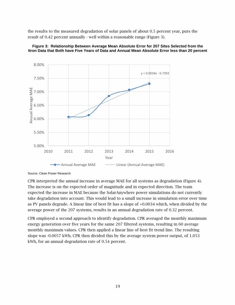
19

the results to the measured degradation of solar panels of about 0.5 percent year, puts the

result of 0.42 percent annually - well within a reasonable range (Figure 3).

Figure 3: Relationship Between Average Mean Absolute Error for 207 Sites Selected from the Itron Data that Both have Five Years of Data and Annual Mean Absolute Error less than 20 percent

Source: Clean Power Research

CPR interpreted the annual increase in average MAE for all systems as degradation (Figure 4).

The increase is on the expected order of magnitude and in expected direction. The team

expected the increase in MAE because the SolarAnywhere power simulations do not currently

take degradation into account. This would lead to a small increase in simulation error over time

as PV panels degrade. A linear line of best fit has a slope of +0.0034 which, when divided by the

average power of the 207 systems, results in an annual degradation rate of 0.32 percent.

CPR employed a second approach to identify degradation. CPR averaged the monthly maximum

energy generation over five years for the same 207 filtered systems, resulting in 60 average

monthly maximum values. CPR then applied a linear line of best fit trend line. The resulting

slope was -0.0057 kWh. CPR then divided this by the average system power output, of 1.053

kWh, for an annual degradation rate of 0.54 percent.

y = 0.0034x - 6.7393

5.00%

5.50%

6.00%

6.50%

7.00%

7.50%

8.00%

2010 2011 2012 2013 2014 2015 2016

An

uu

al A

vera

ge M

AE

Year

Annual Average MAE Linear (Annual Average MAE)

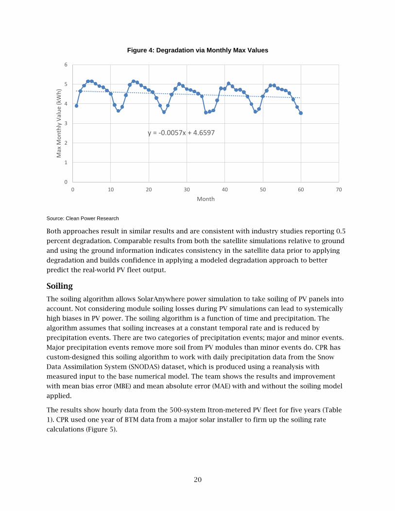
20

Figure 4: Degradation via Monthly Max Values


Both approaches result in similar results and are consistent with industry studies reporting 0.5

percent degradation. Comparable results from both the satellite simulations relative to ground

and using the ground information indicates consistency in the satellite data prior to applying

degradation and builds confidence in applying a modeled degradation approach to better

predict the real-world PV fleet output.

Soiling

The soiling algorithm allows SolarAnywhere power simulation to take soiling of PV panels into

account. Not considering module soiling losses during PV simulations can lead to systemically

high biases in PV power. The soiling algorithm is a function of time and precipitation. The

algorithm assumes that soiling increases at a constant temporal rate and is reduced by

precipitation events. There are two categories of precipitation events; major and minor events.

Major precipitation events remove more soil from PV modules than minor events do. CPR has

custom-designed this soiling algorithm to work with daily precipitation data from the Snow

Data Assimilation System (SNODAS) dataset, which is produced using a reanalysis with

measured input to the base numerical model. The team shows the results and improvement

with mean bias error (MBE) and mean absolute error (MAE) with and without the soiling model

applied.

The results show hourly data from the 500-system Itron-metered PV fleet for five years (Table

1). CPR used one year of BTM data from a major solar installer to firm up the soiling rate

calculations (Figure 5).

y = -0.0057x + 4.6597

0

1

2

3

4

5

6

0 10 20 30 40 50 60 70

Max

Mo

nth

ly V

alu

e (k

Wh

)

Month

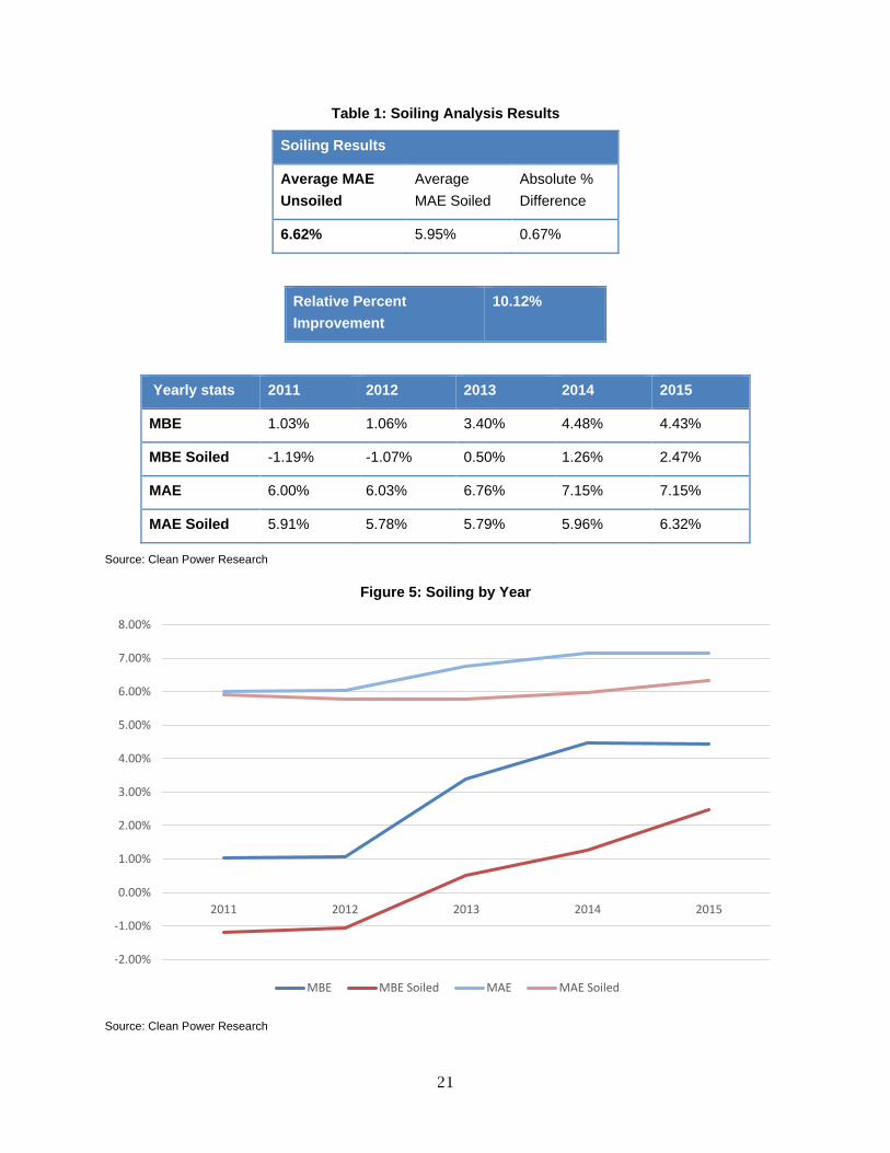
21

Table 1: Soiling Analysis Results

Soiling Results

Average MAE

Unsoiled

Average

MAE Soiled

Absolute %

Difference

6.62% 5.95% 0.67%

Relative Percent

Improvement

10.12%

Yearly stats 2011 2012 2013 2014 2015

MBE 1.03% 1.06% 3.40% 4.48% 4.43%

MBE Soiled -1.19% -1.07% 0.50% 1.26% 2.47%

MAE 6.00% 6.03% 6.76% 7.15% 7.15%

MAE Soiled 5.91% 5.78% 5.79% 5.96% 6.32%


Figure 5: Soiling by Year


-2.00%

-1.00%

0.00%

1.00%

2.00%

3.00%

4.00%

5.00%

6.00%

7.00%

8.00%

2011 2012 2013 2014 2015

MBE MBE Soiled MAE MAE Soiled

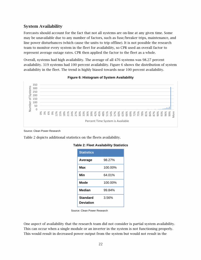
22

System Availability

Forecasts should account for the fact that not all systems are on-line at any given time. Some

may be unavailable due to any number of factors, such as fuse/breaker trips, maintenance, and

line power disturbances (which cause the units to trip offline). It is not possible the research

team to monitor every system in the fleet for availability, so CPR used an overall factor to

represent average outage rates. CPR then applied the factor to the fleet as a whole.

Overall, systems had high availability. The average of all 476 systems was 98.27 percent

availability. 319 systems had 100 percent availability. Figure 6 shows the distribution of system

availability in the fleet. The trend is highly biased towards near 100 percent availability.

Figure 6: Histogram of System Availability


Table 2 depicts additional statistics on the fleets availability.

Table 2: Fleet Availability Statistics

Statistics

Average 98.27%

Max 100.00%

Min 64.01%

Mode 100.00%

Median 99.84%

Standard

Deviation

3.56%


One aspect of availability that the research team did not consider is partial system availability.

This can occur when a single module or an inverter in the system is not functioning properly.

This would result in decreased power output from the system but would not result in the

050

100150200250300350

0%

3%

6%

9%

12

%

15

%

18

%

21

%

24

%

27

%

30

%

33

%

36

%

39

%

42

%

45

%

48

%

51

%

54

%

57

%

60

%

63

%

66

%

69

%

72

%

75

%

78

%

81

%

84

%

87

%

90

%

93

%

96

%

99

%

Mo

re

Nu

mb

er o

f Sy

stem

s

Percent Time System is Available

23

system be reported as unavailable, rather it might be interpreted as degradation or soiling.

Since the system is not reporting zeros, this aspect of availability remains unmeasured. This

partial availability would be seen in increased error between the power simulations, and actual

ground data. This error would be difficult to systematically identify.

Additionally, CPR investigated the relationship between system size and availability. CPR

hypothesized that larger systems have a higher availability because they are more likely to be

carefully monitored and maintained. Figure 7 shows that relationship, however the sample size

is small enough that this relationship may be obscured. Finally, the available data skewed

heavily towards single family residential systems.

Figure 7: Availability as a Function of System Size


Improving System Specifications by Inference

With more than 5 GW of utility-scale PV capacity, the California ISO’s ability to forecast output

from large PV plants is becoming increasingly important.3 CPR has learned that detailed system

specifications improve the accuracy of modeled PV output. Unfortunately, these specifications

are difficult to obtain because most of these plants are privately owned. It is CPR’s hypothesis

that it should be possible to use historical weather data and measured system output to infer

some or all of a PV system’s specifications automatically. The same approach might also be

used to determine BTM system specifications.

The goal for this part of the project was to develop a command-line tool that would compare

measured PV production data with the simulated output from candidate systems with various

3 http://www.eia.gov/todayinenergy/detail.php?id=24852.

y = -2.2701x + 8.8581

0

10

20

30

40

50

60

70

60% 65% 70% 75% 80% 85% 90% 95% 100% 105%

Syst

em S

ize

(kW

)

Availabilty

24

tilt and azimuth combinations. It would then identify the candidate system whose output

resulted in the best fit to the measured data.

To simplify the problem somewhat, exact system location (latitude and longitude) is a required

input. Also, the first version of the tool would only attempt to infer tilt, azimuth, and

alternative current (AC) and direct current (DC) system ratings for fixed (that is non-tracking)

systems. Furthermore, to reduce the overall error in candidate system output, CPR used a

baseline specification would provide any known system details such as commissioning date,

row count, row spacing, or solar obstructions.

CPR obtained measured PV production data for the period from March 1, 2013 through March

31, 2014 for several utility-scale PV plants. The team focused on three of the smaller plants,

designated Plant A, B, and C. CPR used publicly available information to determine actual plant

specifications manually. CPR supplemented this information with satellite imagery to determine

the approximate number of rows of modules, number of inverters, and the array orientation.

CPR used that information as the basis for a baseline system to be used as a template for each

of the candidate systems whose simulated output would be compared to measured.

Figures 8 shows measured output for two of the PV plants studied. Based on the increases in

maximum power output, it appears that the plant was undergoing construction from March

through July 2013. Starting in August 2013, maximum power output remains flat, in spite of

seasonal changes that would normally cause a drop-in output. From this, it can be deduced that

the plant has a DC to AC ratio high enough to allow its maximum power output to remain

relatively constant throughout the year.

Figure 8: Measured Photovoltaic Output, Example One


CPR has clipped the plant’s output shown in Figure 9 due to a high DC to AC ratio. However,

the ratio is not high enough to permit its maximum power output to remain constant

throughout the year and there is a drop in maximum power output from October through

January. Also worth noting is the lack of data in mid-January 2014. This could be either a

reporting error or a plant outage. It is impossible to know from the measured data alone.

25

Figure 9: Measured Photovoltaic Output, Example Two


These two measured data examples illustrate some of the challenges in deriving system

specifications from measured data: Changes in plant capacity, inverter clipping and lack of

seasonal output changes due to high DC to AC ratios, missing data, and unknown PV plant

operational status.

When automatically inferring specifications, the tool correctly identified the gross capacity

changes over time but had difficulty during transitional periods where capacity changed on an

almost daily basis. Once capacity had stabilized, the simulated output from the selected

candidate system matched the measured output reasonably well (Figure 10).

Figure 10: Measured and Simulated Photovoltaic Output for Selected Days, Example One


For the output, CPR slightly underestimated the AC capacity by the spec inference tool (Figure

11) and overestimated the DC to AC ratio (Figure 12).

26

Figure 11: AC Capacity Underestimated, Example Two


Figure 12: DC to AC Ratio Overestimated, Example Two


Table 3 summarizes the system specifications inferred for three sets of measured data.

Information about these three systems was readily available online for these systems and in

two cases, the baseline system yielded the lowest relative mean absolute error. However, the

process identified a much better candidate for Plant A, reducing error significantly.

27

Table 3: Summary of Results for Three Systems


Clean Power Research made significant progress in creating an automated tool for inferring PV

system specifications using measured PV output data. Due to the complexities inherent in

interpreting such data, the team believes that additional accuracy is possible. For example, the

project team did not account for solar obstructions, soiling, module degradation and other

factors that decrease DC output. Consideration of such details were outside of the scope of this

project, but the team hopes to continue development of this tool and the algorithms it

implements.

CPR could apply preliminary versions of the tool when implemented in software to a system

that improves the quality of reported PV system specifications in PowerClerk (the system of

record for PV specifications under CSI), by incorporating measured production data from PV

systems within a utility or ISO territory.

Other Forecast Improvements

Inverter Power Curve

Historically, when modeling PV system output, CPR has relied on the Energy Commission-

weighted average efficiency rating to determine the output of an inverter relative to its DC

input. CPR has used this single number in conjunction with an inverter power curve that is the

Plant A Plant B Plant C

Baseline

Rating (MW DC-PTC) 7.733 19.668 20.703

Rating (MW AC with Losses) 6.821 17.347 18.260

Tracking none (fixed) none (fixed) none (fixed)

Azimuth 180 180 180

Tilt 20 20 20

DC to AC Ratio 1.22 0.98 0.98

rMAE 23.0% 12.6% 12.8%

Selected Candidate

Rating (MW DC-PTC) 7.772 19.668 20.703

Rating (MW AC with Losses) 7.402 17.347 18.260

Tracking none (fixed) none (fixed) none (fixed)

Azimuth 180 180 180

Tilt 25 20 20

DC to AC Ratio 1.05 0.98 0.98

rMAE 6.2% 12.6% 12.8%

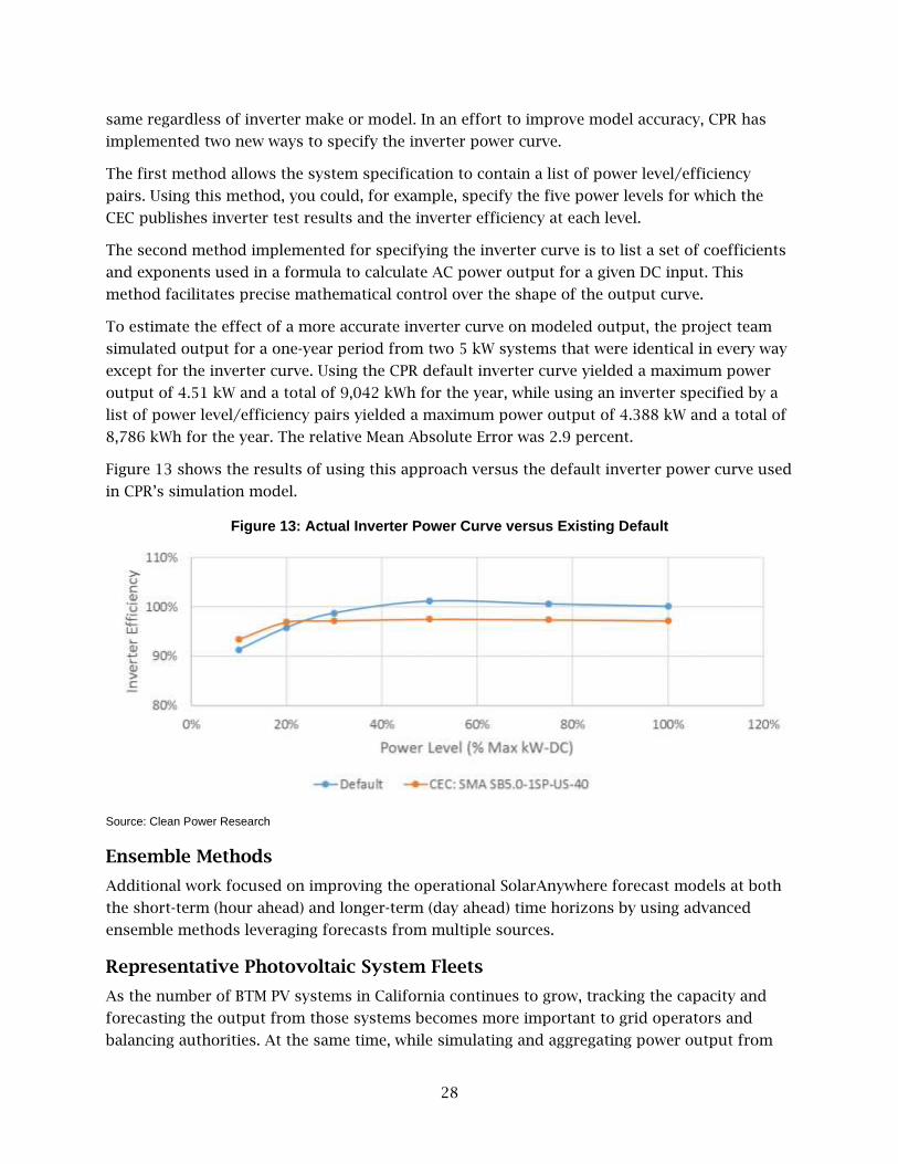
28

same regardless of inverter make or model. In an effort to improve model accuracy, CPR has

implemented two new ways to specify the inverter power curve.

The first method allows the system specification to contain a list of power level/efficiency

pairs. Using this method, you could, for example, specify the five power levels for which the

CEC publishes inverter test results and the inverter efficiency at each level.

The second method implemented for specifying the inverter curve is to list a set of coefficients

and exponents used in a formula to calculate AC power output for a given DC input. This

method facilitates precise mathematical control over the shape of the output curve.

To estimate the effect of a more accurate inverter curve on modeled output, the project team

simulated output for a one-year period from two 5 kW systems that were identical in every way

except for the inverter curve. Using the CPR default inverter curve yielded a maximum power

output of 4.51 kW and a total of 9,042 kWh for the year, while using an inverter specified by a

list of power level/efficiency pairs yielded a maximum power output of 4.388 kW and a total of

8,786 kWh for the year. The relative Mean Absolute Error was 2.9 percent.

Figure 13 shows the results of using this approach versus the default inverter power curve used

in CPR’s simulation model.

Figure 13: Actual Inverter Power Curve versus Existing Default


Ensemble Methods

Additional work focused on improving the operational SolarAnywhere forecast models at both

the short-term (hour ahead) and longer-term (day ahead) time horizons by using advanced

ensemble methods leveraging forecasts from multiple sources.

Representative Photovoltaic System Fleets

As the number of BTM PV systems in California continues to grow, tracking the capacity and

forecasting the output from those systems becomes more important to grid operators and

balancing authorities. At the same time, while simulating and aggregating power output from

29

individual systems provides greater accuracy, it also requires ever-increasing computing

resources. However, CPR can combine system capacity from multiple systems in nearby

locations with similar orientations to create representative systems, thereby reducing the

number of simulations of distinct systems in a fleet while retaining the diversity of locations

and orientations that characterize the fleet’s power production. While these “Representative PV

Fleets” introduce some level of error into the modeling process, the decrease in simulation time

may prove to be a worthwhile trade-off. In addition, CPR could apply representative fleet

concepts in a top-down manner to extrapolate PV fleet production in areas where the detailed

specification of individual resources is unknown.

CPR produced BTM PV fleet power forecasts every 30 minutes for five load regions4 in the

territories of California’s three investor-owned utilities (IOUs). The California ISO identified these

five load regions. CPR produced these forecasts using satellite-derived irradiance values from

SolarAnywhere at 1 km x 1 km spatial resolution. CPR used system specifications such as latitude,

longitude, tilt and azimuth, PV module and inverter efficiency ratings, obtained from IOUs, the

Energy Commission and CSI, to model power output from approximately 186,000 systems. CPR

aggregated the power output from these individual systems to provide fleet power output.

These systems, however, only represent about 43 percent of the total systems online.

According to the CPUC California Solar Statistics web site,5 homeowners and businesses have

installed more than 440,000 behind the meter PV systems in California IOU territories. That

number appears to be growing steadily, with more than 30 percent of the systems installed in

2015 (Figure 14).

Figure 14: Cumulative Installed Behind-the meter Systems in California


4 These regions are SDG&E, SCE Inland, SCE Coastal, PG&E Bay Area, and PG&E Non-Bay Area.

5 https://www.californiasolarstatistics.ca.gov/.

30

In addition to the increased computing horsepower required to model such large numbers of

systems, specifications for the systems in the publicly available data are inexact or missing

altogether. For example, locations are anonymized by providing only the systems’ zip code.

Furthermore, system orientation (tilt and azimuth) is only available for 30 percent of the

systems. Rather than creating generic systems and guessing at their orientation and exact

location, the team scaled the modelled PV fleet power output on the assumption that the

locations and system orientations of new systems will have a distribution similar to that of the

current fleet captured in PowerClerk. In a way, this is one of the simplest methods for creating

a bottom-up representative PV fleet.

Method

To investigate methods for reducing the computational resources required for modelling large

PV fleets and to better quantify the margin of error that generalizing the locations and

orientation of systems in such fleets might introduce, CPR created various representative fleets

using the CSI systems in the PG&E Non-Bay Area load region behind-the-meter fleet as a

baseline for comparison. CPR spread this baseline fleet, consisting of the 34,562 PV systems,

across a large portion of California and has a wide variety of system orientations. CPR

simulated the 30-minute power output from each of these systems for a one-year period from

January 1, 2014 through December 31, 2014 and aggregated results to produce the baseline

fleet output every 30 minutes during the period. CPR binned the capacity in a baseline fleet

with known system specifications to create “Bottom-up” representative fleets. CPR calculated

the relative Mean Absolute Error (rMAE)6 for each of the representative (test) fleets to compare

to the output of this baseline (reference) fleet.

Geographic Bin Selection

CPR selected site locations for the representative fleets using one of two methods. In the first

method, CPR created a grid, by evenly dividing the rectangle bounding the systems in the

baseline fleet. The method used six different spatial resolutions. The first five spatial

resolutions tested were 1.6° latitude and longitude (approximately 160 x 160 kilometers), 0.8°,

0.4°, 0.2°, and 0.1° latitude and longitude (approximately 10 x 10 kilometers).

CPR mapped capacity for each system to the nearest location on the grid, then further binned

by orientation (tilt, azimuth, and tracking). Error! Reference source not found. shows the s

elected geographic bins and how

CPR combined them with the orientation bins (described in the next section) to create the

systems in each representative fleet. The map in Figure 15 shows the locations for one

representative fleet. Each location included multiple systems, sized to represent the capacity of

the actual systems in each orientation bin.

6 Thomas E. Hoff, J. K. (2012). Reporting of Irradiance Model Relative Errors. Proc. ASES Annual Conference. Raleigh, NC:

American Solar Energy Society.

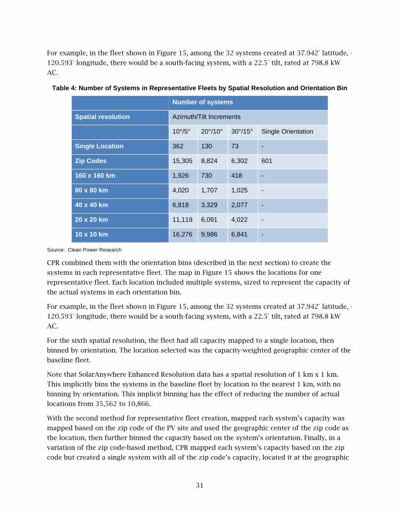
31

For example, in the fleet shown in Figure 15, among the 32 systems created at 37.942° latitude, -

120.593° longitude, there would be a south-facing system, with a 22.5° tilt, rated at 798.8 kW

AC.

Table 4: Number of Systems in Representative Fleets by Spatial Resolution and Orientation Bin

Number of systems

Spatial resolution Azimuth/Tilt Increments

10°/5° 20°/10° 30°/15° Single Orientation

Single Location 362 130 73 -

Zip Codes 15,305 8,824 6,302 601

160 x 160 km 1,926 730 418 -

80 x 80 km 4,020 1,707 1,025 -

40 x 40 km 6,818 3,329 2,077 -

20 x 20 km 11,119 6,091 4,022 -

10 x 10 km 16,276 9,986 6,841 -


CPR combined them with the orientation bins (described in the next section) to create the

systems in each representative fleet. The map in Figure 15 shows the locations for one

representative fleet. Each location included multiple systems, sized to represent the capacity of

the actual systems in each orientation bin.

For example, in the fleet shown in Figure 15, among the 32 systems created at 37.942° latitude, -

120.593° longitude, there would be a south-facing system, with a 22.5° tilt, rated at 798.8 kW

AC.

For the sixth spatial resolution, the fleet had all capacity mapped to a single location, then

binned by orientation. The location selected was the capacity-weighted geographic center of the

baseline fleet.

Note that SolarAnywhere Enhanced Resolution data has a spatial resolution of 1 km x 1 km.

This implicitly bins the systems in the baseline fleet by location to the nearest 1 km, with no

binning by orientation. This implicit binning has the effect of reducing the number of actual

locations from 35,562 to 10,866.

With the second method for representative fleet creation, mapped each system’s capacity was

mapped based on the zip code of the PV site and used the geographic center of the zip code as

the location, then further binned the capacity based on the system’s orientation. Finally, in a

variation of the zip code-based method, CPR mapped each system’s capacity based on the zip

code but created a single system with all of the zip code’s capacity, located it at the geographic

32

center of the zip code, and used the baseline fleet’s capacity-weighted azimuth and tilt (17° and

175°, respectively) as that system’s orientation.

Figure 15: Representative Fleet with System Locations at 0.4° Latitude/Longitude Spacing


Orientation Bin Selection

In addition to binning system capacity by location, when creating the representative fleets, CPR

binned the capacity of the actual systems by tilt, azimuth and tracking to capture the diversity

in system orientations at each location typical in large PV fleets. System orientation bins were

based on 10° azimuth and 5° tilt increments (648 bins), 20°, azimuth and 10° tilt increments (162

bins), or 30° azimuth and 15° tilt increments (72 bins). Dual-axis tracking systems, where

azimuth and tilt vary continuously throughout the day, constituted an additional bin.

For each location, CPR assigned the capacity for each array7 to the bin that most closely

matched the azimuth and tilt of that array. For example, in the case where CPR used 30°

azimuth and 15° tilt increment bins, capacity for arrays with azimuths that were +/- 15° from

7 CPR analyzed capacity at the array level rather than the system level to properly account for

systems with multiple arrays.

33

south (165° to 195°) with tilts between 22.5° and 37.5° it would have added to the 180°

azimuth/30° tilt capacity bin.

System Creation and Simulation

CPR determined the total capacity for each location/orientation bin and created systems with

the appropriate capacity. Table 4 shows the number of systems in each of the 22 representative

fleets created by combining spatial and orientation bins.

CPR calculated the maximum power rating for the inverter used for each system based on the

capacity-weighted DC to AC ratio for the baseline fleet of 1.027 as recorded for actual systems.

CPR set inverter efficiency for each system to 96.2 percent - also based on the capacity-

weighted inverter efficiency rating of the baseline fleet – and set other DC losses to 11 percent -

once again using the capacity-weighted DC losses of the baseline fleet. After creating the

systems, CPR simulated power output for each system for every 30-minute period from January

1, 2014 through December 31, 2014 and aggregated the results to produce 30-minute interval

fleet power. CPR then compered those results to the output from the baseline fleet.

Effect of Spatial Resolution and Orientation Bin Count on Relative Mean Absolute Error

The amount of error introduced by using bottom-up representative PV fleets with regular

geographic dispersion, rather than fleets consisting of individual systems with exact system

specifications varied from 4.2 percent for the coarsest spatial resolution and smallest number

of orientation bins, to 1.1 percent for the fleet with 10 km x 10 km spatial resolution and the

largest number of orientation bins. As shown in Figure 16, the greatest impact on error was due

to spatial resolution, rather than the number of orientations considered. However, further

increases in spatial resolution would likely have proportionally less impact.

The rMAE for the representative fleets with a single location had significantly higher error than

the other fleets, ranging from 10.1 percent to 10.7 percent.

The representative fleet based on multiple orientations at each zip code fared reasonably well

with rMAE ranging from 2.2 percent to 2.4 percent. However, the zip code-based fleet that used

a single orientation at each zip code had a much higher rMAE at 6.6 percent. While a multi-

orientation zip code-based fleet may be appropriate when exact system locations are unknown,

performance is only slightly better than the representative fleets with the highest number of

orientation bins and spatial resolution, and error is approximately double.

The graphs in Figure 17 show the correlation between the 30-minute power values for selected

representative fleets versus the baseline fleet. At the same spatial resolution, there was little

difference between fleets with different numbers of orientation bins, so CPR omitted these.

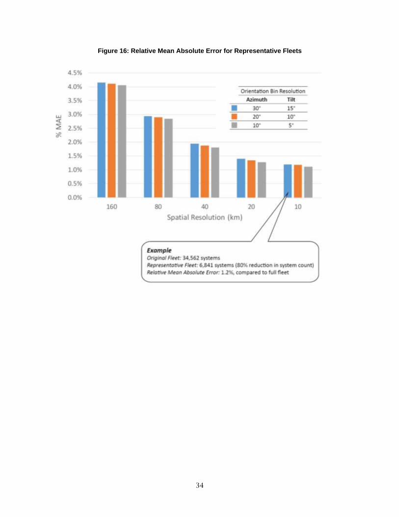
34

Figure 16: Relative Mean Absolute Error for Representative Fleets

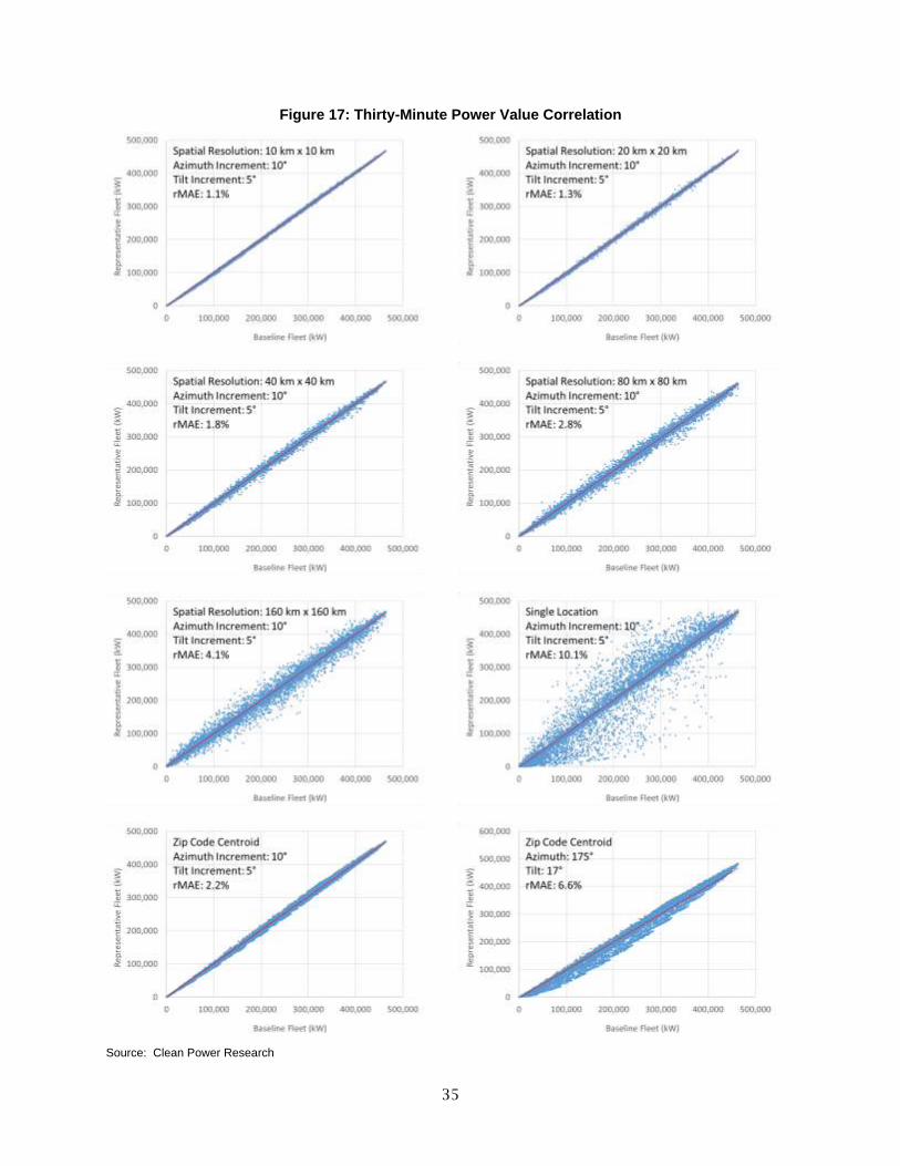
35

Figure 17: Thirty-Minute Power Value Correlation


36

Performance Benefits

In general, the amount of time it takes to simulate a PV fleet scales linearly with the number of

simulated systems. CPR found that when there are many systems to be simulated at a single

location, there is approximately an 8 percent additional reduction in time. Although CPR

tracked simulation times for the representative and baseline fleets, the team believes that the

actual times, which vary greatly depending on computer system load and data transmission

speeds over the Internet, should not be considered when evaluating performance. Instead,

based on the number of locations and systems, Table 5 shows the hypothetical reduction in

time required to simulate these representative fleets relative to the baseline fleet. Even at the

highest spatial resolution and the largest number of orientation bins evaluated, CPR reduced

the simulation times by 63.5 percent. However, fewer orientation bins at the same high spatial

resolution adds only 0.1 percent error, while yielding an 83.4 percent reduction in simulations

time.

Table 5: Estimated Reduction in Simulation Times for Representative Fleets Relative to Baseline Fleet

Azimuth/Tilt Increments

10°/5° 20°/10° 30°/15° Single Orientation

Single Location 99.2% 99.7% 99.8%

Zip Codes 66.3% 80.0% 85.3% 98.6%

160 x 160 km 95.9% 98.4% 99.1%

80 x 80 km 91.4% 96.3% 97.7%

40 x 40 km 85.5% 92.9% 95.5%

20 x 20 km 75.7% 86.3% 90.7%

10 x 10 km 63.5% 76.8% 83.4%


Using bottom-up representative PV fleets, created by generalizing the location and orientation

of a set of individual systems with known specifications, can reduce computing resource

requirements by more than 80 percent in modelling fleet output, while introducing as little as

1.2 percent rMAE on an annual basis. By applying scaling factors to the known historical

California BTM PV fleet, this was the approach used for the trial of this project with California

ISO.

Zip code based representative fleets, which make use of known individual system orientation

data can reduce computing resource requirements by more than 65 percent, while introducing

as little as 2.2 percent rMAE on an annual basis.

Representative fleets that make use of a single location exhibit more than 10 percent rMAE and

have a fairly inaccurate power production curve on a daily basis, despite short simulation

37

times. At 6.6 percent rMAE, zip code fleets that use a single system orientation have less error

than single location fleets, but typically exhibit a narrower daily production curve with a higher

peak. CPR found that it is necessary to account for loss of accuracy and ensure that any

avoidable error is not introduced when applying this approach correctly as the size of the PV

fleet continues to grow.

Dynamic Regional Fleet Capacity Updates

The equipment comprising BTM PV systems do not always remain in service on a continuous

basis. Owners sometimes replace system components such as the inverter. They also may add

or remove modules. They sometime built utility-scale systems in phases, with capacity growing

over time. In addition, outages – both planned and unplanned – can cause capacity to drop. As

part of this project, CPR has implemented the ability to track changes in system capacity over

time and use that information when simulating system output.

California leads the nation in BTM PV installations – systems whose production, for the most

part, utilities do not track. To provide an accurate estimate of the power produced by these

systems, it is important to have detailed information about each system’s configuration:

location, installation date, orientation of each array in the system, the model’s and quantities of

installed modules and inverters, and the elevation of any solar obstructions, such as buildings

and trees surrounding the system that are above the bottom edge of the panels. Modeling

software produces a reasonably accurate estimate of the system’s production8 when combined

with accurate weather data, whether historical or forecast

Beginning in 2007, PowerClerk collected detailed specifications for systems incentivized under

the CSI, an online software service from CPR. CPR also collected specifications for non-CSI BTM

systems incentivized under Self Generation Incentive Program (SGIP), the Emerging Renewables

Program (ERP). By the end of 2014, CPR team had collected detailed specifications for more

than 140,000 CSI systems and 43,000 non-CSI systems. CPR used these system specifications,

with a combined capacity over 2.1 GW, in the creation of five of the BTM fleets used in the

California ISO forecast.

As incentives available through the CSI began to run out, utilities gradually discontinued

tracking interconnections in PowerClerk. This was especially true in PG&E and SDG&E

territories, and CPR began to look for ways to keep the capacity of its PV fleets up to date.

Initially, CPR experimented with capacity data provided to California ISO by the IOUs. However,

the poor quality (for example redundant and missing data) of data prevented its use. Next, the

project team obtained market research data from GTM Research. Although the data quality was

better, reporting was only by quarter for the entire state, rather than by IOU or region.

In July 2015, the CPUC began posting monthly editions of the net energy metered (NEM)

Currently Interconnected Data Set (CIDS) on the California Solar Statistics web site.9 This data

8 https://www.nrel.gov/analysis/sam/pdfs/2008_sandia_ieee_pvsc.pdf.

9 http://www.californiadgstats.ca.gov/downloads/.

38

set is useful for estimating total installed capacity. However, it is of limited usefulness as a

source for detailed system specifications due to anonymized locations (only zip codes) and

missing data (tilt and azimuth) is available for only 30 percent of the systems. Figure 18 shows

the capacity of the systems tracked in CSI (“FleetView”) and systems recorded in the CIDS

database (“CPUC Net Energy Metering (NEM) Data”).

Figure 18: California Behind-the meter Fleet Capacity 2008 to 2016


By using capacity data from the NEM Interconnection Applications Data Set in conjunction with

the detailed system specifications in FleetView, CPR was able to develop the time-dependent

scaling factors and apply them to the historical simulations of the five California ISO BTM

fleets. Itron used the simulation output to train its load forecasting software. Furthermore,

FleetView now automatically recalculates the scaling factors when the CPUC publishes CIDS

updates, then projects to future dates and applies to the California ISO BTM fleet forecasts.

Determination of Fleet Historical Scaling Factors

Since CPR believes the NEM CIDS contains only those systems that are currently online, and not

decommissioned, CPR evaluated the NEM Interconnection Applications Data Set to get a

complete picture of historical capacity over time. Figure 18 depicts the complete picture of

historical capacity.

Determination of Fleet Forecast Scaling Factors

For forecasting, CPR derived a linear formula for the scaling factor growth trend for each

California ISO zonal fleet, defined by this project, using CIDS and FleetView capacities for the

most recent two months. CPR dynamically calculates monthly scaling factors using those

formulas, based on the time elapsed since the beginning of the growth trend period and applied

to the PV production forecast. Technically, coefficients only need to be updated if the growth

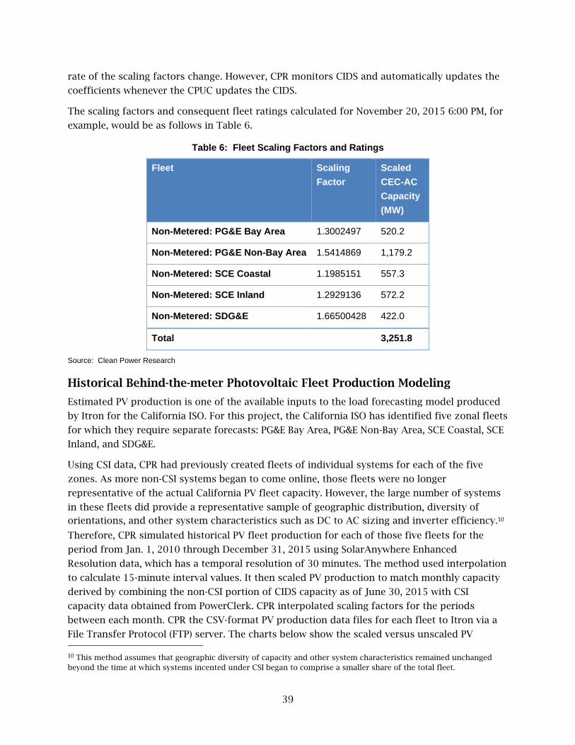
39

rate of the scaling factors change. However, CPR monitors CIDS and automatically updates the

coefficients whenever the CPUC updates the CIDS.

The scaling factors and consequent fleet ratings calculated for November 20, 2015 6:00 PM, for

example, would be as follows in Table 6.

Table 6: Fleet Scaling Factors and Ratings

Fleet Scaling

Factor

Scaled

CEC-AC

Capacity

(MW)

Non-Metered: PG&E Bay Area 1.3002497 520.2

Non-Metered: PG&E Non-Bay Area 1.5414869 1,179.2

Non-Metered: SCE Coastal 1.1985151 557.3

Non-Metered: SCE Inland 1.2929136 572.2

Non-Metered: SDG&E 1.66500428 422.0

Total 3,251.8


Historical Behind-the-meter Photovoltaic Fleet Production Modeling

Estimated PV production is one of the available inputs to the load forecasting model produced

by Itron for the California ISO. For this project, the California ISO has identified five zonal fleets

for which they require separate forecasts: PG&E Bay Area, PG&E Non-Bay Area, SCE Coastal, SCE

Inland, and SDG&E.

Using CSI data, CPR had previously created fleets of individual systems for each of the five

zones. As more non-CSI systems began to come online, those fleets were no longer

representative of the actual California PV fleet capacity. However, the large number of systems

in these fleets did provide a representative sample of geographic distribution, diversity of

orientations, and other system characteristics such as DC to AC sizing and inverter efficiency.10

Therefore, CPR simulated historical PV fleet production for each of those five fleets for the

period from Jan. 1, 2010 through December 31, 2015 using SolarAnywhere Enhanced

Resolution data, which has a temporal resolution of 30 minutes. The method used interpolation

to calculate 15-minute interval values. It then scaled PV production to match monthly capacity

derived by combining the non-CSI portion of CIDS capacity as of June 30, 2015 with CSI

capacity data obtained from PowerClerk. CPR interpolated scaling factors for the periods

between each month. CPR the CSV-format PV production data files for each fleet to Itron via a

File Transfer Protocol (FTP) server. The charts below show the scaled versus unscaled PV

10 This method assumes that geographic diversity of capacity and other system characteristics remained unchanged

beyond the time at which systems incented under CSI began to comprise a smaller share of the total fleet.

40

production for each of the five California ISO fleets. As illustrated in Figure 19, CPR’s estimate

of non-CSI capacity in the SCE Coastal Region before 2014 was higher than that reported in the

CIDS. These results assume that the CIDS is the best source for capacity available.

Figure 19: Southern California Edison Coastal Photovoltaic Production


Robustness of the California Independent System Operator Forecast Delivery

To improve availability and accuracy of the forecasts provided to California ISO during this

project, CPR made the following operational changes to the forecast production and delivery:

1. Add distributed processing support to process larger fleets more quickly.

2. Run forecasts on a scalable cloud-based platform that permits better monitoring and

increases reliability.

3. Automatically detect changes to the NEM Currently Interconnected Data Set and, trigger

an automatic update of the scaling factors applied to the baseline fleet output.

Real-time Data Feedback

The use of feedback from real time production data have the potential to also improve

forecasts. By using the current conditions and knowledge of the clear sky profile, it would be

possible to advance the current observed clearness index along the clear sky profile to produce

a “persistence forecast.” This assumes that the cloud conditions will not vary from the current

conditions, or in other words that the current conditions will persist. However, it is difficult to

obtain real time data, fast enough to produce a forecast and disseminate for decision making.

The approach taken in this project was to focus on the use of production data from distributed

rooftop systems. This requires a large number of systems, particularly if the systems did not

report data reliably, were out of service, or they were reporting bad data. These are all possible

factors for distributed systems.

Itron provided near real-time access to data from approximately 30 systems in the Bay Area.

Time delay in the readings was inevitable: the process required data transmission from the PV

41

system itself to Itron’s database, followed by ingesting into the forecast system. CPR developed

and demonstrated a proof-of-concept system for retrieving and ingesting the data, and the

process typically took 20 minutes when working correctly.

CPR demonstrated the process for a period of about one month. The system used real time data

to modify the CPR solar forecast. During this period, CPR evaluated the modified forecasts and

observed small forecast improvements in the modified forecast of PV system power for each of

the 30 PV systems. CPR expected this since it proved that persistence, at least for short time

scales, adds skill to the forecast. However, for forecasts beyond three hours CPR observed no

improvement in forecast skill.

After a month, the cellular carrier phased out support of the modems that collected the data.

This prevented a comprehensive evaluation. The use of data from these distributed systems is

also costly, so a more complete evaluation would not only have to determine whether a forecast

improvement was possible on a consistent basis, but also whether any such improvement

would justify ongoing maintenance costs at scale. CPR is not clear how many systems would

provide a meaningful impact state-wide. A more complete evaluation could become cost-

prohibitive.

42

Chapter 4: Improving Short-term Load Forecasts by Incorporating Solar Photovoltaic Generation

Background

Itron developed the load forecasts that the California ISO relies on for real-time system

operations using statistical models of five-minute measured loads. The California ISO collects

these data in real time based on measurement points at each grid-connected generation

resource, as well as, inter-region tie lines. It is important to note that at the time of this study,

the California ISO does not measure either in real time or ex post BTM solar PV generation. This

means measured load does not equal actual end-user (that is, residential, commercial,

industrial, agriculture, and other customer segments) consumption of electricity, since BTM

solar PV generation supplies some portion of the consumption.

The net effect of a deep penetration of BTM solar PV is that forecasts of measured load are

becoming less reliable. This is especially true in the morning hours because the presence of

clouds (for example, marine layer) rather than temperatures appear to drive loads. In contrast,

temperature changes that drive air conditioning loads appear to dominate afternoon loads. This

may change over time when BTM solar PV penetration reaches a critical mass, where the

variation in BTM solar PV generation is sufficiently large to outweigh the load variation due to

variation in air conditioning loads.

The California ISO must extend the existing load forecast models to capture the influence of

BTM solar PV and better predict an increasing volatile load. This study evaluates three

alternative model approaches for extending the California ISO load forecast framework. This

report presents the alternative load forecast frameworks for incorporating BTM solar PV

forecasts and the forecast simulations that Itron implemented to evaluate the performance of

these approaches.

To put these approaches into context, following is a description of the existing California ISO

load forecast model.

California Independent System Operator Short-Term Load Forecast Model

Itron used the Baseline Load Forecast Model provide forecasts of measured loads for forecast

horizons of 15 minutes ahead out to ten days ahead. The California ISO load forecasting system

produces 15-minute level load forecasts for forecast horizons of 15-minutes ahead out ten (10)

days ahead. The load forecasts update automatically every 15-minutes to support generation

scheduling and dispatching. A separate set of load forecast models are used for each of the

three major California ISO load zones: PG&E, SCE and SDG&E. In addition, the California ISO

develops sub-region forecasts for five (5) climatic zones: PGE& Bay Area, PG&E Non-Bay Area,

SCE Coastal, and SCE Inland load zones and SDG&E. Hourly weather forecasts of temperature

43

and humidity for approximately 24 weather stations located throughout the State of California

drive the load forecasts. Itron updated the weather forecasts hourly from multiple weather

forecast service providers.

For each load zone (PG&E, PG&E Bay Area, PG&E Non Bay Area, SCE, SCE Inland, SCE Coastal,

and SDG&E), the baseline 15-minute load forecast modeling framework is composed of 193

individual forecast models. The 193 individual forecast models that define the California ISO

baseline 15-minute load forecast modeling framework are:

1. Daily energy model. Itron used a Neural Network Model of Daily Energy to capture daily

swings in electricity demand as driven by changes in calendar and weather conditions.

2. Day-ahead models. Designed for forecast horizons of four hours ahead and longer.

Composed of 96, 15-Minute Regression Models driven by the forecasts from the Daily

Energy Model, as well as by forecasted calendar and weather conditions. Because the

Day-Ahead models do not contain autoregressive terms, they are quick to react to

changing weather conditions.

3. Hour-ahead models. Designed for forecast horizons of up to four to six hours ahead. Is

composed of a second set of 96, 15-Minute Regression Models that launch off the most

recent meter data through inclusion of autoregressive terms in addition to forecasted

calendar and weather conditions.

Itron updated the operational forecast that the California ISO utilizes every 15 minutes which

has a forecast horizon of the balance-of-the-day out ten days ahead. Itron created a single

quarter hour load forecast by taking a weighted average of the Day-Ahead and Hour-Ahead

forecasts. For forecast horizons of up to two hours ahead, Itron placed 100 percent weight on

the Hour-Ahead forecasts. Between two and four hours ahead, the weight cascades away from

the Hour-Ahead forecast and towards the Day-Ahead forecast. For forecast horizons of four

hours ahead and longer, Itron placed 100 percent weight on the Day-Ahead forecast.

This framework offers the following advantages over the use of a single set of 96, quarter hour

models.

1. Forecasts of daily energy capture the influence of a full day of weather conditions on

loads. Itron channeled this influence through to the Day-Ahead model forecasts via

predicted daily energy values with day-of-the-week interaction terms.

2. The day-ahead model forecasts are free to respond quickly to forecasted changes in

weather conditions.

3. The hour-ahead models exploit the information contained in the most recent metered

loads.

4. The blended forecast balances the value of autoregressive terms over near-term forecast

horizons with the value of forecasted weather conditions over longer-term forecast

horizons in a single forecast.

44

A total of eight separate models make up this framework. The Task 4 full report11 provides a

more detailed description of the California ISO’s forecasting models.

The Impact of Solar Photovoltaic on the California Independent System

Operator Short-Term Load Forecast

The statistical models described above use linear least squares to estimate the model

coefficients. At a very high level, the process of estimating the model coefficients is an

averaging of the historical load data, where the explanatory variables segment the load data

over which Itron takes the averages. While this is not an exact description of the least squares

approach, it is a useful metaphor when describing how solar PV impacts the estimated

coefficients of the California ISO short-term load forecast models. Over time, an increased

penetration of solar PV has the net effect of reducing on average measured load. This implies

that the estimated model coefficients embody this reduction in measured loads. That is, Itron

tunes the model coefficients to measured load under average solar PV production that occurred

over the model estimation period. As a result, the short-term load forecasts produce a forecast

under average solar PV production conditions. The challenge is on any given day actual solar PV

production will not necessarily align with the average solar PV production. On cloudy days

when solar PV production is smaller than average, the load forecast will under forecast loads

because the model fails to reflect the bump up in loads due to lower solar PV production. On

sunny days when solar PV production is greater than average, the load forecast will over

forecast loads because the model fails to reflect the drop-in loads due to higher solar PV

production.

The issue is that a statistical model of measured load will capture the average impact of solar

generation in the estimated model coefficients. Accordingly, with volatile solar PV generation,

Itron adjusts the model-based forecast of measured load to account for the solar PV generation

not already accounted for by the estimated model coefficients. A key objective of this study is

to develop a means for improving the short-term load forecast by incorporating forecasts of

solar PV generation into the forecast framework. The next section describes three alternative

frameworks for incorporating the impact of solar PV generation into a forecast of measured

loads.

Incorporating the Impact of Solar Photovoltaic Generation in a Load Forecast

The existing California ISO short-term load forecast models do not include explicit treatment of

solar PV generation. As such, the forecasts are subject to the type of forecast bias described

above. In particular, the existing California ISO mid-day forecasts tend to be high on sunny days

and low on cloudy days. This study developed alternative forecast frameworks that account for

the load impact of solar PV generation. The study uses forecast simulations to compare the

11 Monforte, Dr. Frank A.; Fordham, Christine; Blanco, Jennifer; Barsun, Stephan (Itron, Inc.) Kankiewicz, Adam; Norris,

Ben (Clean Power Research). 2016. Improving Short-Term Load Forecasts by Incorporating Solar PV Generation. California Energy Commission, https://www.energy.ca.gov/2017publications/CEC-500-2017-031/CEC-500-2017-031.pdf.

45

forecast accuracy of the existing California ISO forecast framework against the three alternative

modeling approaches; Error Correction, Reconstituted Loads, and Model Direct.

What follows is a brief description of these three frameworks.

Error Correction

The Error Correction approach implements what many System Operators do initially when

faced with the problem of solar PV generation. Namely, they make ex post adjustments of the

load forecast to account for forecasted values of solar PV generation. On sunny days, Itron

lowers the load forecast and on cloudy days, Itron adjusts the load forecast upward. The key

advantage of the Error Correction Approach is that Itron can continue to use the existing load

forecast model without any changes. All Itron needs is a means of forecasting solar PV

generation. This report describes the framework below.

Day-Ahead Error Correction Forecast. The Day-Ahead Error Corrections recognize that the

Day-Ahead model coefficients capture the average amount of solar PV generation that existed

over the model estimation period. Since the load forecast already reflects a certain level of

solar PV generation the ex post error correction makes an adjustment based on how much the

current solar PV generation differs from the historical average solar PV generation.

In this case, if the forecast of solar PV generation is higher than the historical average, then

Itron adjusts the Day-Ahead Load Forecast downward. For example, on a clear sunny day, Itron

adjusts the Day-Ahead Load Forecast downward to account for greater than average solar PV

generation. On the other hand, on cloudy days when solar PV generation forecasts are lower

than the historical average, Itron adjusts the Day-Ahead Load Forecast upwards.

Hour-Ahead Error Correction Forecast. The Hour-Ahead Forecast models are highly

autoregressive. In principle, this means the Measure Load values passed into the models as

autoregressive terms reflect a certain amount of solar PV generation. For example, the load

forecast made at 11:00 for 11:15 launches off measured loads at 11:00, 10:45, 10:30, 10:15, and

10:00. If it is a sunny day, these measured loads are lower than average due to the higher than

average solar PV generation. Conversely, on a cloud day these measured loads are higher than

average due to a lower than average solar PV generation. If at 11:15 one expects that the solar

PV generation is going to be higher than what it was at 11:00, then one would want to adjust

down the Hour-Ahead Forecast. On the other hand, if one expects that there will be a drop in

solar PV generation between 11:00 and 11:15, the Hour-Ahead Forecast should be lifted.

This approach uses the difference of forecasts of solar PV generation to make the error

correction because real-time measurement of solar PV generation does not exist. Real-time

measurement data makes it possible to use measured values instead of forecast values.

Error Corrected Measured Load Forecast. Itron constructed the Error Corrected Measured Load

Forecast as a weighted average of the Error Corrected Hour-Ahead and Day-Ahead forecasts.

46

Reconstituted Loads

Itron reconstitutes the historical time series of measured load under the Reconstituted Loads

approach by adding back estimates of solar PV generation. Itron then re-estimates the load

forecast model against the reconstituted loads. Itron adjusts the subsequent reconstituted load

forecasts ex post by subtracting away forecasts of solar PV generation to form a forecast of

measured loads. By estimating the model coefficients against a time series of demand for

power regardless of how it is sourced, one controls for any inherent bias on the estimated

coefficients of a model of measured loads. The disadvantage is one must develop and maintain

an historical time series of solar PV generation to estimate the load forecast model coefficients.

Further, this approach assumes that the historical solar PV generation time series is accurate.

This may not necessarily be true, in which case this approach places too high of a weight on the

solar PV generation values.

This approach uses the difference of forecasts of solar PV generation to make the error

correction because real-time measurement of solar PV generation does not exist. If real-time

measurement data become available, then the measured value replaces forecast value.

Model Direct

Under this approach, one directly estimates the weight placed on the solar PV generation data

by including these data as an explanatory variable in the load forecast models. The estimated

coefficient on the solar PV generation variable is the weight. Also, in principle, no bias on the

remaining explanatory variables should be introduced by including solar PV generation as an

explanatory variable. This approach also provides a direct forecast of measured loads that

accounts for solar PV generation, thus avoiding any ex post processing of the load forecast. Like

the Reconstituted Load Approach, this approach requires developing and maintaining an

historical time series of solar PV generation.

Solar Photovoltaic Generation Estimates

This study uses two alternative sources for solar generation to evaluate the forecast

performance of the Error Correction, Reconstituted Loads, and Direct Modeling approaches

described above. CPR developed the first source of solar generation data and a detailed

database of solar installations in the PG&E, SCE, and SDG&E service territories. The second

source of solar generation mimics what a number of system operators have used as starting

point for addressing the impact of solar generation on their loads, which is to leverage the

cloud cover data they already collect. Under this approach, Itron combines the hourly cloud

cover data collected by weather stations with estimates of installed capacity to estimate solar

generation by load zone. The purpose of developing this second source is to provide a basis for

comparison to the forecast improvements when the solar generation estimates/forecasts come

from a commercial vendor like CPR.

Clean Power Research Solar Generation Estimates

Much of the solar generation forecasting focus is on developing accurate forecasts of panel-

level solar irradiance. The techniques range from vector decomposition of satellite imagery to

47

vector decomposition of location specific cloud cover observations. Itron has geared this

analysis for forecasting generation at utility solar installations and/or solar generation over a

small geographic footprint. This micro focus is most useful when the exact locations of the

solar installations are known. For the case of the California ISO, CPR has combined this micro

level approach with a detailed database of solar PV installations to construct a rich time series

of non-utility scale solar generation estimates by load zone. Itron used these estimates to

evaluate the forecast performance of the alternative load forecast approaches described above.

Increased penetration of solar PV can lead to growing load volatility that in turn will lead to

eroding load forecast performance. To put the solar generation data derived by CPR into a load

forecasting context, it is useful to consider what fraction of load volatility could be associated

with solar generation volatility. Figure 20 presents the ratio of solar generation volatility to load

volatility for the total PG&E service territory. Here, Itron measured the solar generation

volatility by the standard deviation (stdkwh) of the estimated solar generation output

(solargenkwh), gold area in the chart, by time interval. Itron measured the load volatility by the

standard deviation of loads (red area in the chart) by time interval. The green line in Figure 20

is the ratio of these two volatility measures. For the case of PG&E. the ratio of solar generation

volatility to PG&E load volatility peaks around 10 am at a value of 0.22. This is in stark contrast

to SCE (Figure 21), which also peaks mid-morning but at a much lower value of 0.13. As shown

in Figure 22, SDG&E has a similar volatility profile as PG&E, with the ratio of solar generation

volatility to SDG&E load volatility peaking mid-morning with a value of 0.20. Figure 23 presents

a comparison the ratios for PG&E, SCE, and SDG&E.

From a model perspective, the greater the proportion of load volatility that can be associated

with or explained by the volatility of solar generation, the more improvement in model fit that

one can expect when adding solar generation as an explanatory variable in a model. To help fix

ideas, consider a simple analogy of trying to measure (predict) the depth of a lake. If the lake is

relatively shallow, accurately predicting the height of the waves is relatively important. In

contrast, wave height is noise when considering trying to measure the depth of a lake as deep

such as Lake Tahoe. In load forecasting, the volatility of solar generation is the measurement of

the height of the waves. The load volatility is the measurement of the depth of the lake. The

smaller the ratio of solar volatility (that is, the waves) to load volatility (depth of the lake) the

less weight a statistical model will place on the solar generation variables. As a result, it is less

likely that adding forecasts of solar generation will improve the load forecast. Conversely, the

higher the ratio the more likely one will have forecast performance gains from adding forecasts

of solar generation to the model.

The data in Figure 23 suggest that the forecast performance improvements were less for SCE

than for PG&E and SDG&E because of the lower ratio. Further, Itron anticipated that there would

be bigger performance gains in the mid-morning hours than the afternoon hours. Finally, Itron

expected little to no forecast gains for the dawn and dusk hours when solar generation output

was at its lowest.

48

Figure 20: Ratio of Solar Generation Volatility to Load Volatility (Pacific Gas & Electric Total)


In this and subsequent figures, “stdkwh” is the estimated load variability (using the Standard

Deviation of Measured Loads in MW), “solargenkwh” is the estimated solar PV generation

variability (using Standard Deviation of BTM solar PV generation in MW), and “Ratio” is the ratio

of solargenkwh to stdkwh.

Cloud Cover Driven Solar Generation Estimates

Unfortunately, not all system operators have access to the detailed installation data that CPR

has gathered for the state of California. In many cases, a system operator will have at best good

estimates of the total installed capacity by transmission zone and/or possibly by postal code.

Further, most system operators only have access to hourly cloud cover data for the weather

stations they use to forecast loads. For years, load forecasters have lived by the assumption

that hourly weather data for a handful of weather stations was sufficient to produce accurate

short-term load forecasts. This begs the question, is having an estimate of total installed

capacity by transmission zone coupled with hourly cloud cover data for a handful of weather

stations that span the load zone sufficient to capture the overall impact of solar PV generation

on loads?

To answer this question, Itron developed an alternative time series of solar PV generation by

combining the total installed solar PV capacity estimates by load zone developed by CPR with

the hourly cloud cover observations for the weather stations that the California ISO uses to

49

drive their load forecasts. The result was a time series of solar PV generation for the load

zones: PG&E, PG&E Bay Area, PG&E Non Bay Area, SCE, SCE Coastal, SCE Inland, and SDG&E.

Figure 21: Ratio of Solar Generation Volatility to Load Volatility: Southern California Edison Total


Figure 22: Ratio of Solar Generation Volatility to Load Volatility: San Diego Gas & Electric


50

Figure 23: Ratio of Solar Generation Volatility to Load Volatility: Investor-owned Utility Comparison


One can quantify the benefit of doing “something” over doing “nothing” by comparing the

forecast performance of the short-term load forecasts with and without cloud cover driven

solar PV generation. Further, one can establish a baseline of short-term load forecast

performance against which the short-term load forecast using CPR’s detail bottom-up solar PV

generation estimates can be evaluated. The remainder of this section, Itron describes how to

develop forecasts (estimates) of solar PV generation by load zone by combining hourly cloud

cover with solar PV capacity estimates.

Itron’s approach used to develop cloud cover solar PV generation estimates was necessarily

simple given the limited information available:

• Total Installed solar PV capacity (MW) by day and load zone, and

• Hourly Cloud Cover in percentage terms by hour, day and weather station.

Listed below are the practical steps used to develop the historical time series of solar PV

generation by load zone.

Step 1. Construct an Historical Time Series of Solar Insolation. Given the above engineering

relationship, how does one predict the amount of solar energy that will reach the surface of a

51

solar panel for any location and time? For this study, Itron used the National Oceanic &

Atmospheric Administration (NOAA) solar calculation spreadsheet12 to derive estimates of solar

insolation by location and day of year for roughly the geographic midpoint (measured as

latitude/longitude) for the following load zones: PG&E Bay Area, PG&E Non Bay Area, SCE

Coastal, SCE Inland and SDG&E. This step provided daily estimates of solar insolation at Solar

Noon for the period January 1, 2010 through December 31, 2015.

To compute a value of solar insolation for a specific time-of-the-day, it is important to know the

Solar Altitude Angle for that time point. Again, Itron used the information available on the

NOAA spreadsheet which gives an estimate of the time of Solar Noon that corresponds to a

Solar Altitude Angle of 90 degrees. This spreadsheet also provides estimated sunrise and

sunset times. Since the Solar Altitude Angle at the time of sunrise and sunset is 0 degrees, one

can back into the average decay per minute in the Solar Altitude Angle.

Step 2. Constructing Estimates of Solar PV generation Capacity. For this study, Itron used the

CPR-developed historical time series of solar installations by load zone to develop the solar PV

generation estimates.

Step 3. Cloud Cover Driven Solar PV Generation. Next, Itron used hourly cloud cover and

temperature values from the weather stations assigned to each load zone to derive estimates of

solar PV generation which it will use in the load forecasting models. Figure 24 through Figure

28 present a comparison of the Cloud Cover solar generation estimates to the CPR estimates for

the week of May 24, 2015. In general, the CPR estimates are smoother than the Cloud Cover

driven estimates. This reflects the data smoothing inherent in the bottom-up approach

implemented by CPR versus the hourly choppiness that comes with hourly cloud cover

observations for a small number of weather stations. Itron anticipated that the smoother CPR

estimates would lead to less volatile measured load forecasts than the cloud-cover driven

estimates. If this observation proves true, then that is a distinct advantage of the CPR approach

because adding load forecast uncertainty is not desirable.

12 http://www.esrl.noaa.gov/gmd/grad/solcalc/calcdetails.html

52

Figure 24: CPR versus Cloud Cover Solar Generation (MWh): Pacific Gas & Electric Bay Area


Figure 25: CPR versus Cloud Cover Solar Generation (MWh): Pacific Gas & Electric Non Bay Area


53

Figure 26: CPR versus Cloud Cover Solar Generation (MWh): Southern California Edison Coastal


Figure 27: CPR versus Cloud Cover Solar Generation (MWh): Southern California Edison Inland


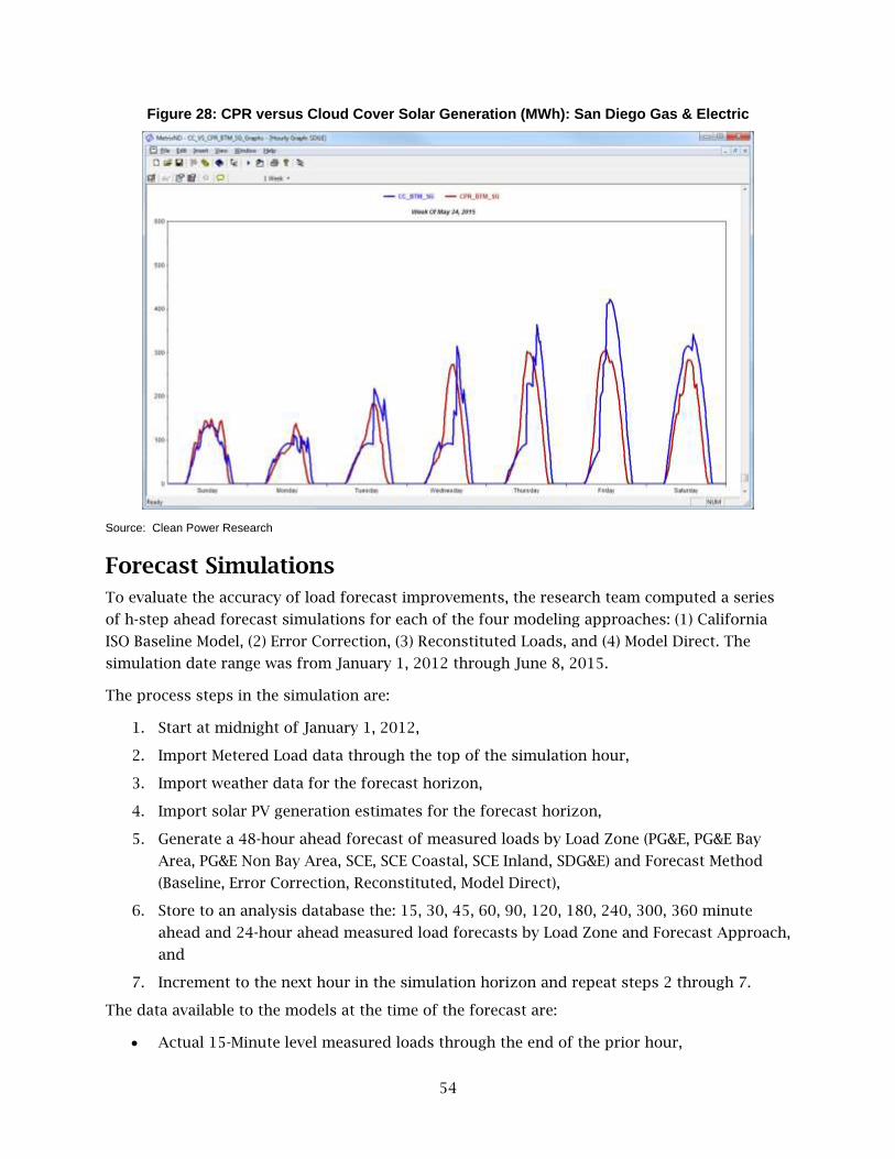
54

Figure 28: CPR versus Cloud Cover Solar Generation (MWh): San Diego Gas & Electric


Forecast Simulations

To evaluate the accuracy of load forecast improvements, the research team computed a series

of h-step ahead forecast simulations for each of the four modeling approaches: (1) California

ISO Baseline Model, (2) Error Correction, (3) Reconstituted Loads, and (4) Model Direct. The

simulation date range was from January 1, 2012 through June 8, 2015.

The process steps in the simulation are:

1. Start at midnight of January 1, 2012,

2. Import Metered Load data through the top of the simulation hour,

3. Import weather data for the forecast horizon,

4. Import solar PV generation estimates for the forecast horizon,

5. Generate a 48-hour ahead forecast of measured loads by Load Zone (PG&E, PG&E Bay

Area, PG&E Non Bay Area, SCE, SCE Coastal, SCE Inland, SDG&E) and Forecast Method

(Baseline, Error Correction, Reconstituted, Model Direct),

6. Store to an analysis database the: 15, 30, 45, 60, 90, 120, 180, 240, 300, 360 minute

ahead and 24-hour ahead measured load forecasts by Load Zone and Forecast Approach,

and

7. Increment to the next hour in the simulation horizon and repeat steps 2 through 7.

The data available to the models at the time of the forecast are:

• Actual 15-Minute level measured loads through the end of the prior hour,

55

• Hourly observed weather data by weather station for all weather concepts, including:

Temperature, Dew Point, Cloud Cover, Wind Speed, and Wind Direction, and

• Estimated (Forecasted) 15-Minute level solar PV generation.

Itron used observed weather conditions to eliminate load forecast error driven by weather

forecast errors.

The research team used the two sets of estimated solar PV generation in the simulations: (a)

cloud cover driven and (b) CPR detailed bottom-up estimates. The use of cloud cover based

solar generation estimates mimic the initial approach many system operators have

implemented as a first pass at trying to improve their eroding load forecasts. A comparison of

the results from the different estimates should demonstrate the benefit of the more detailed

approach implemented by CPR.

Forecast Performance Measurements

A common metric used to evaluate load forecast performance is the Mean Absolute Percentage

Error (MAPE). This metric represents the average percentage error in absolute terms expected

from a load forecast model. In general, load forecast MAPEs become bigger the longer the

forecast horizon.

To facilitate identifying improvements in forecast performance relative to the baseline forecast

the forecast MAPE values represent the percentage change relative to the baseline MAPE. In this

case, a negative percent change in the forecast MAPE of the alternative approach represents an

improvement in forecast performance over the baseline forecast.

A second metric for evaluating forecast accuracy improvements is Forecast Skill. This is a

commonly used statistic in renewable energy forecasting studies, which tend to compare the

performance of an alternative approach relative to a baseline approach such as a persistence

forecast. Forecast Skill metrics also avoid a problem inherent in the use of MAPE for evaluating

the forecast performance of solar and wind generation that occurs when the observed

generation value run close to zero. Small generation values tend to be associated with large

percentage forecast errors not necessarily because there are large absolute forecast errors, but

rather the error is divided by a small number.

For this study, Forecast Skill measures the percentage of forecast simulations that the

candidate forecast approach produced, a smaller in absolute terms load forecast error than the

baseline load forecast. In this case, if the Forecast Skill is greater than 50 percent of the time, a

forecast approach will lead to an improvement on average in load forecast accuracy.

These first two metrics focus on the first moment of the forecast error distribution. In addition

to reducing forecast errors on average, Itron was interested in testing whether or not the

alternative forecast approaches reduce the overall dispersion of forecast errors. In this case,

Itron measured the forecast error dispersion using the Forecast Standard Deviation.

To ease comparisons, Itron constructed the change in the Standard Deviation of the forecast

errors of each approach relative to the baseline Standard Deviation. In this case, a negative

56

percent change in the forecast Standard Deviation of the alternative approach represents an

improvement in forecast performance over the baseline forecast.

Collectively, the team looked to evaluate whether or not the alternative approaches reduced not

only the mean or average forecast error, but also the dispersion of forecast errors.

Simulation Results Summary

The results of forecast simulations for January 1, 2015 through June 30, 2015 are below. Itron

selected this period since it represents the most recent data and the period which PV

installations were at their highest. The results from earlier periods are less applicable to the

forecast problem currently faced by the California ISO because the earlier periods had

significantly lower penetration of PV relative to 2016 values.

The exhibits present the forecast MAPE, Skill, and Error Standard Deviation by:

• Forecast Horizon

o 15 Minutes Ahead

o 30 Minutes Ahead

o 45 Minutes Ahead

o 60 Minutes Ahead

o 90 Minutes Ahead

o 120 Minutes Ahead (2 Hours Ahead)







• Forecast Approach

o Baseline Load Forecast Model with no Behind-the-Meter Solar Generation

o Error Correction Approach using Cloud Cover driven Solar Generation estimates

o Model Direct Approach using Cloud Cover driven Solar Generation estimates

o Reconstituted Loads Approach using Cloud Cover driven Solar Generation estimates

o Error Correction Approach using CPR’s Solar Generation estimates

o Model Direct Approach using CPR’s Solar Generation estimates

o Reconstituted Loads Approach using CPR’s Solar Generation estimates

The results are presented for the following segmentations:

• Load Zones:

57

o California ISO Total

o PG&E Bay Area

o PG&E Non Bay Area

o SCE Coastal

o SCE Inland

o SDG&E Total

• Seasons:

o Winter (October through March)

o Summer (April through September)

• Cloud Cover Conditions

o Clear: average cloud cover percentage less than 75 percent

o Cloudy: average daily cloud cover percentage greater than or equal to 75 percent

Figure 29 through Figure 40 summarize the results. On each figure, the values highlighted in

green represent an improvement over the baseline load forecast.

California Independent System Operator Total Simulation Results

• Figure 29 through Forecast Horizons of 12 Hours Ahead to 24 Hours Ahead. For longer-

term forecast horizons of 12 hours ahead to 24 hours ahead, the Reconstituted Load

approach combined with CPR solar generation estimates significantly reduced both the

forecast MAPE and error dispersion. Over this same forecast horizon, the Error

Correction approach combined with either Cloud Cover or CPR solar generations

estimates outperformed the baseline load forecast. This suggests that imposing an a

priori weight of -1.0 on the solar generation estimates works well for these longer

forecast horizons.

• Seasonal Differences. The conclusions do not change substantially when the forecast

results are segmented between the winter and summer seasons. The Model Direct

approach utilizing the CPR solar generation estimates improves the load forecast

performance for forecast horizons of 15 minutes ahead to five hours ahead. For longer

forecast horizons, the Reconstituted Load approach out performs the baseline load

forecast. The main difference between the seasonal results and the overall results is the

Model Direct approach using Cloud Cover driven solar generation estimates only

performed well during the summer season while this approach performed well for

forecast horizons from 15 minutes ahead to four hours ahead over the winter season.

• Cloud Cover. The alternative approaches appear to work best under varying cloud

conditions. Most notably, combining CPR solar generation estimates reduces the

forecast error dispersion across most forecast horizons under the Model Direct and

Reconstituted Load approaches.

58

Figure 30 presents the results for the California ISO total (that is, the sum of all the PG&E, SCE,

and SDG&E zone loads) across all seasons, and cloud cover conditions.

• Improvement over Baseline. A mix or “ensemble” of the different approaches can result

in a reduction in forecast accuracy. Although these improvements are largely in the

single (relative) percentage points, the improvements still have measurable potential

savings to California of approximately $2 million per year. 13

• Forecast Horizons of 15 Minutes Ahead to Four Hours Ahead. For forecast horizons of

up to four hours ahead, the Model Direct approach consistently outperformed the

baseline load forecast model with both a reduced MAPE and smaller dispersion of

forecast errors. Further, the Model Direct approach performed better than the baseline

forecast when using both Cloud Cover and CPR computed solar generation estimates.

However, the Model Direct approach when combined with the CPR solar generation

estimates outperformed the same approach combined with the Cloud Cover driven solar

generation estimates.

• Forecast Horizons of Five Hours Ahead to Six Hours Ahead. For forecast horizons of five

hours ahead to six hours ahead, the results are mixed between the Model Direct

combined with CPR solar generation estimates and the Reconstituted Loads approach

combined with CPR solar generation estimates. Using Forecast Skill as a metric, the

Reconstituted Loads approach outperformed the baseline forecast. However, the

forecast error dispersion grew with this approach.

13 Based on an average annual California ISO load of 26 GW and an average regulation cost of $9/MWh per MacDonald e.

al ‘Demand Response Providing Ancillary Services A Comparison of Opportunities and Challenges in the US Wholesale Markets’, Grid-Interop Forum 2012

59

Figure 29: California Independent System Operator Total, All Seasons, All Cloud Cover Conditions

* Values that represent an improvement over the baseline load forecast are highlighted in green.


60

• Forecast Horizons of 12 Hours Ahead to 24 Hours Ahead. For longer-term forecast

horizons of 12 hours ahead to 24 hours ahead, the Reconstituted Load approach

combined with CPR solar generation estimates significantly reduced both the forecast

MAPE and error dispersion. Over this same forecast horizon, the Error Correction

approach combined with either Cloud Cover or CPR solar generations estimates

outperformed the baseline load forecast. This suggests that imposing an a priori weight

of -1.0 on the solar generation estimates works well for these longer forecast horizons.

• Seasonal Differences. The conclusions do not change substantially when the forecast

results are segmented between the winter and summer seasons. The Model Direct

approach utilizing the CPR solar generation estimates improves the load forecast

performance for forecast horizons of 15 minutes ahead to five hours ahead. For longer

forecast horizons, the Reconstituted Load approach out performs the baseline load

forecast. The main difference between the seasonal results and the overall results is the

Model Direct approach using Cloud Cover driven solar generation estimates only

performed well during the summer season while this approach performed well for

forecast horizons from 15 minutes ahead to four hours ahead over the winter season.


conditions. Most notably, combining CPR solar generation estimates reduces the



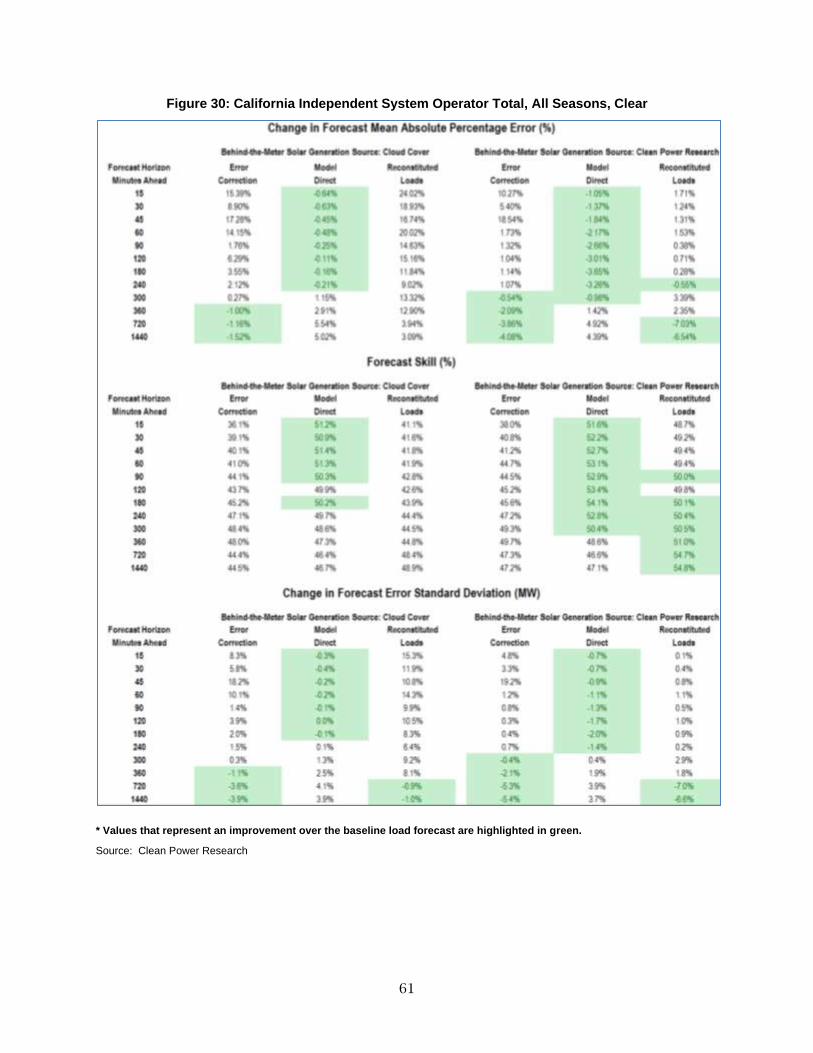
61

Figure 30: California Independent System Operator Total, All Seasons, Clear



62

Pacific Gas & Electric Bay Area Simulation Results

Figure 31 through Figure 32 presents the results for PG&E Bay Area across all seasons, and

cloud cover conditions.





forecast when using both Cloud Cover driven estimates and CPR computed solar

generation estimates. However, the Model Direct approach when combined with the CPR

solar generation estimates outperformed the same approach combined with the Cloud

Cover driven solar generation estimates.


hours ahead to six hours ahead, the Error Correction approach combined with CPR solar

generation estimates outperformed all other approaches.


horizons of 12 hours ahead to 24 hours ahead, the baseline model forecasts were on

average more accurate, but the Error Correction approach combined with the CPR solar

generation estimates led to a tighter distribution of forecast errors.

• Seasonal Differences. The main difference between the winter and summer seasons is

the Model Direct approach when combined with the CPR solar generation estimates

reduced the forecast error dispersion during the winter months across all forecast

horizons. This improvement is limited to the forecast horizons of 15 minutes ahead to

four hours ahead during the summer season.


conditions. Most notably, combining the CPR solar generation estimates reduced the



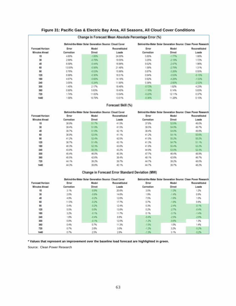
63

Figure 31: Pacific Gas & Electric Bay Area, All Seasons, All Cloud Cover Conditions



64

Figure 32: Pacific Gas & Electric Bay Area, All Seasons, Clear



65

Pacific Gas & Electric Non Bay Area Simulation Results

Figure 33 through Figure 34 presents the results for PG&E Non Bay Area across all seasons, and

cloud cover conditions.










hours ahead to six hours ahead, the Error Correction approach combined with CPR solar



horizons of 12 hours ahead to 24 hours ahead, the baseline model forecasts were on

average more accurate.


the Reconstituted Load approach when combined with the CPR solar generation

estimates performed better with the longer forecast horizons during the summer season

than the winter season.


conditions. Most notably, combining the CPR solar generation estimates reduced the



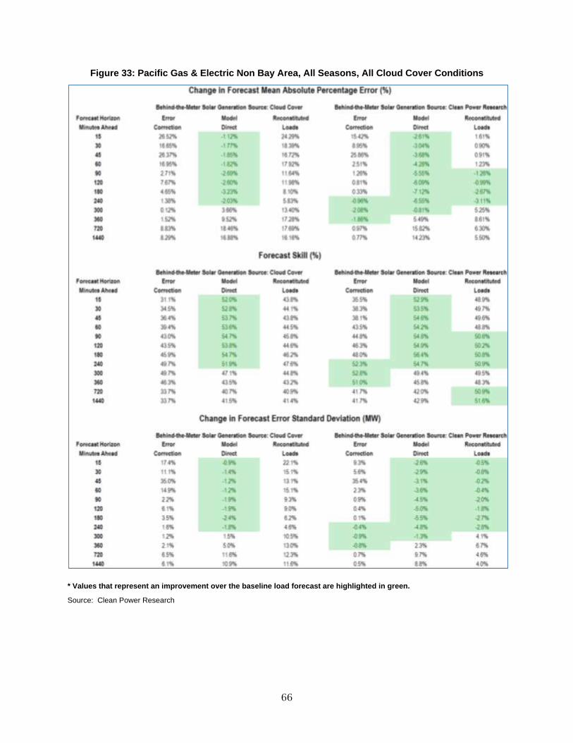
66

Figure 33: Pacific Gas & Electric Non Bay Area, All Seasons, All Cloud Cover Conditions



67

Figure 34: Pacific Gas & Electric Non Bay Area, All Seasons, Clear



68

Southern California Edison Coastal Simulation Results

Figure 35 through Figure 36 presents the results for SCE Coastal across all seasons, and cloud

cover conditions.


one-hour ahead up to four hours ahead, only the Model Direct approach combined with

the CPR solar generation estimates outperformed the baseline load forecast model. For

forecast horizons of less than one-hour ahead the baseline load forecast outperformed

the alternative approaches.


hours ahead to six hours ahead, the Model Direct approach combined with CPR solar



horizons of 12 hours ahead to 24 hours ahead, the Error Correction and Reconstituted

Load approaches were on average more accurate than the baseline load forecast.


the Model Direct approach when combined with the CPR solar generation estimates

performed during the winter season for forecast horizons of 30 minutes ahead to 24

hours ahead. In contrast, the Model Direct approach did not outperform the baseline

model during the summer season across all forecast horizons.

• Cloud Cover. In contrast to other load zones, the alternative approaches appear to work

best under clear cloud conditions. Most notably, the Model Direct approach when

combined with the CPR solar generation estimates outperformed the baseline load

forecast over forecast horizons of 30 minutes ahead to 24 hours ahead.

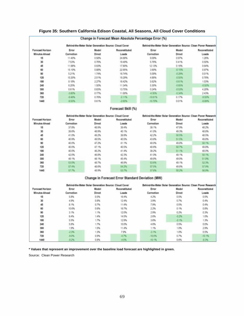
69

Figure 35: Southern California Edison Coastal, All Seasons, All Cloud Cover Conditions



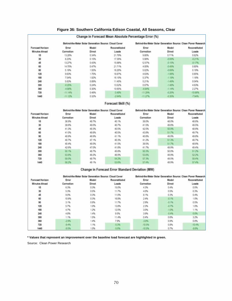
70

Figure 36: Southern California Edison Coastal, All Seasons, Clear



71

Southern California Edison Inland Simulation Results

Figure 37 through Figure 38 presents the results for SCE Inland across all seasons, and cloud

cover conditions.


one-hour ahead up to four hours ahead, only the Model Direct approach combined with

CPR’s and the Cloud Cover driven estimates of solar generation outperformed the

baseline load forecast model.


hours ahead to six hours ahead, the Model Direct approach combined with CPR solar



horizons of 12 hours ahead to 24 hours ahead, the Error Correction and Reconstituted

Load approaches were on average more accurate than the baseline load forecast.


the Error Correction approach when combined with the CPR solar generation estimates

performed well during the summer season, but not so in the winter season.

• Cloud Cover. In general, the alternative approaches combined with the CPR solar

generation estimates worked better under Cloudy conditions.

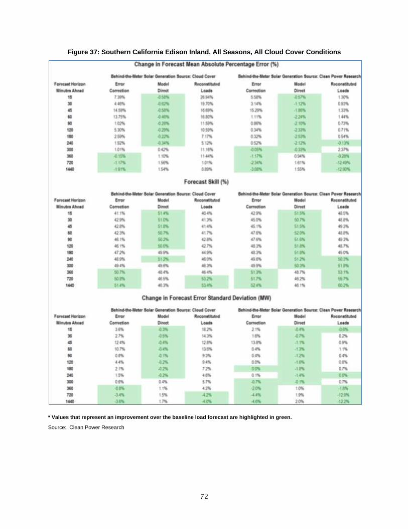
72

Figure 37: Southern California Edison Inland, All Seasons, All Cloud Cover Conditions



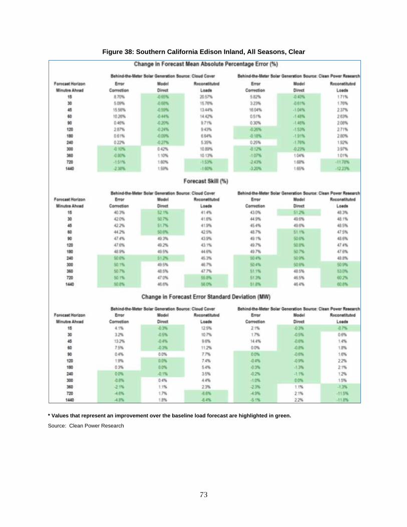
73

Figure 38: Southern California Edison Inland, All Seasons, Clear



74

San Diego Gas & Electric Total Simulation Results

Figure 39 through Figure 40 presents the results for SDG&E across all seasons, and cloud cover

conditions.










hours ahead to six hours ahead, the Model Direct approach combined with both Cloud

Cover driven and CPR solar generation estimates outperformed the baseline load

forecast in terms of both accuracy and reduction of forecast error dispersion.


horizons of 12 hours ahead to 24 hours ahead, again the Model Direct approach

combined with both Cloud Cover driven and CPR solar generation estimates

outperformed the baseline load forecast in terms of both accuracy and reduction of

forecast error dispersion.


that the performance of the Reconstituted Loads approach degrades during the summer

season.

• Cloud Cover. There were no substantial differences between the alternative approaches

performance under cloudy versus sunny conditions.

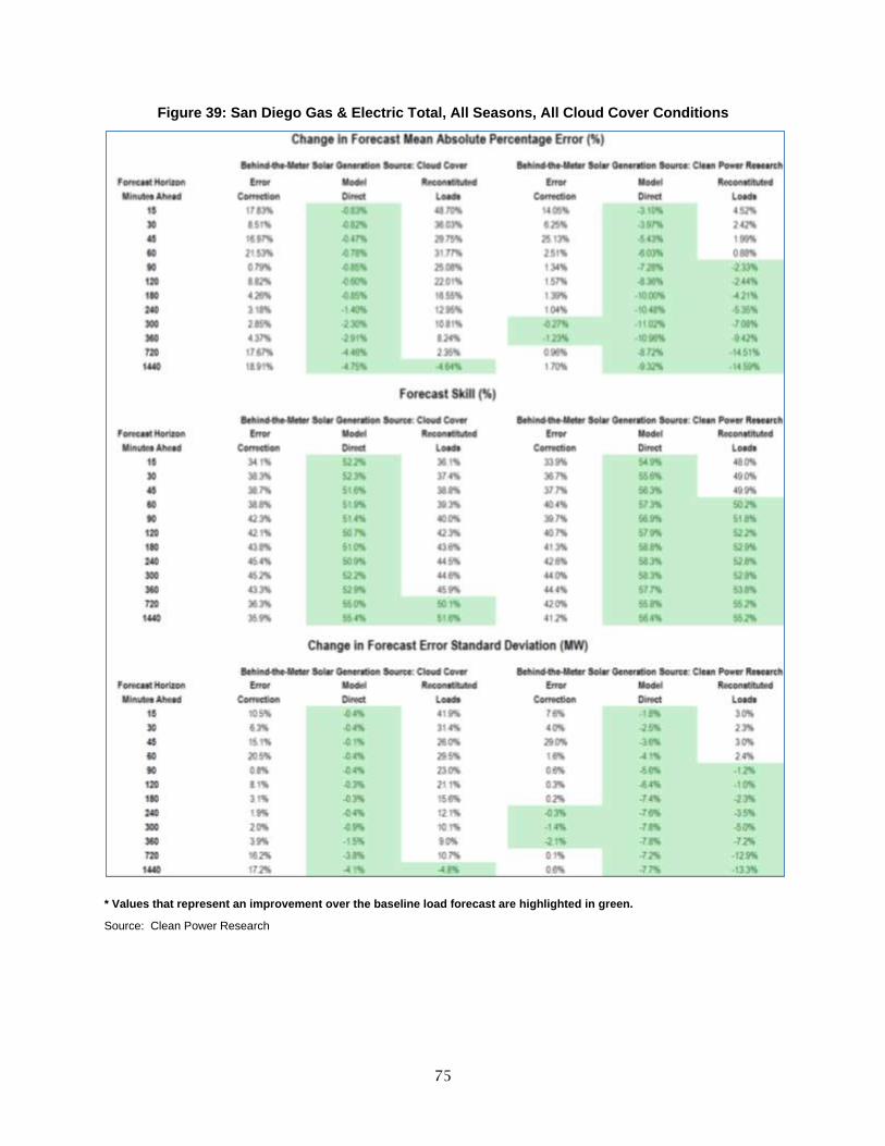
75

Figure 39: San Diego Gas & Electric Total, All Seasons, All Cloud Cover Conditions



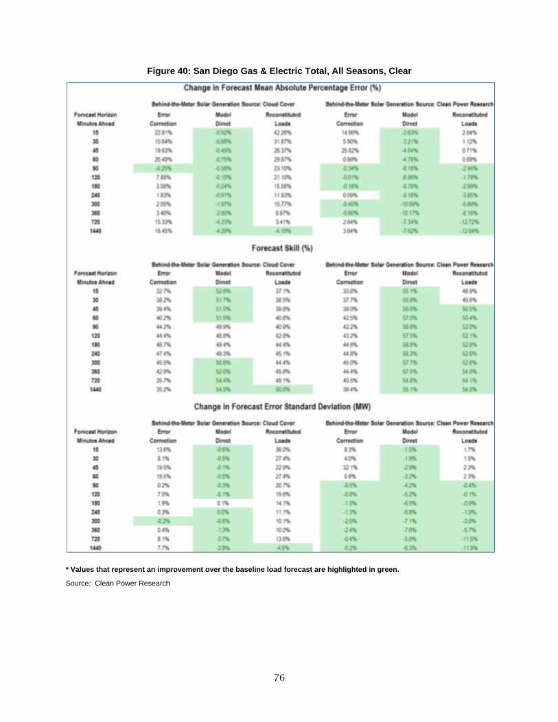
76

Figure 40: San Diego Gas & Electric Total, All Seasons, Clear



77

Statistical Estimates of Solar Photovoltaic Load Impacts

A benefit of the Model Direct approach is that it allows the statistical models through the

process of model estimation to determine the forecasted load impact of a MW of Solar PV

generation. Engineering principles suggest that every 1 MW of Solar PV generation directly

offsets 1 MW of load. Based on these principles, one expects the estimated coefficients on the

Solar PV variables to be equal to or very close to -1.0. In fact, the coefficients on the Solar PV

variables in the Error Correction and Reconstituted Load approaches were explicitly set equal to

-1.0 for just this very reason. Engineering principles, however, do not account for behavioral

changes that may have taken place with the penetration of Solar PV. A plausible behavioral

change is the increased use of air conditioning equipment post installation of Solar PV. Prior to

installing Solar PV, consumers may not have run their air conditioners when they were at work

to save money. Post Solar PV installation, the idea that they now have “free” electricity might

lead consumers to leave their air conditioners on all the time regardless of whether they are

home or not. In this example, 1 MW of Solar PV generation still offsets 1 MW of load, but that

reduction may be masked by a load increase driven by the behavioral change. As a result, one

may not realize an engineering-based a priori value of -1.0 for the estimated coefficient on the

Solar PV variable.

Other confounding factors include prevailing weather conditions and the mix of space heating

and space conditioning that exists in the load zone. A hot, cloudy day may offset the lower

Solar PV generation value with higher air conditioning loads especially in load zones that have

high penetrations of air conditioning. That same hot, cloudy day in an area with low air

conditioning saturations may have the full impact of the Solar PV generation because of the

lack of offsetting air conditioning loads. In a similar fashion, a cold, cloudy morning might lead

to the compounding of a load increase associated with lower Solar PV generation by an increase

in electric space heating loads.

In general, weather and behavioral driven utilization of space conditioning equipment will

complicate the observed load impact of Solar PV generation. Without detailed measurement of

end-use equipment loads, it is difficult for a statistical model to isolate the impact of Solar PV

generation on measured loads. Unfortunately, the challenge of isolating the impact of Solar PV

on measured loads will only become more complex with saturation of electric vehicle charging

and behind-the-meter storage, which will provide consumers flexibility with when they will use

the electricity generated by their solar panels. In this soon-to-be-here world, the 1 MW of solar

generation at Noon may offset 1 MW of vehicle charging at midnight. This type of behavioral

change will further mask the load impact of Solar PV generation.

Presented in Figures 41-44 are the statistically estimated load impacts under average solar and

maximum solar conditions for the California ISO total and each of the load zones. In the

figures, the dashed yellow line represents CPR’s estimate of maximum Solar PV generation over

the 2014-2015 period. The blue dashed line represents CPR’s estimate of average Solar PV

Generation over the same period. The solid gold line is the statistically adjusted maximum

Solar PV generation impact that Itron computed as the product the CPR’s maximum Solar PV

generation and the estimated coefficient on the Solar PV variable from each of the 96 Day-

78

Ahead models. The solid blue line is the statistically adjusted average Solar PV generation

impact that Itron computed as the product the CPR’s average Solar PV generation and the

estimated coefficient on the Solar PV variable from each of the 96 Day-Ahead models.

Figure 41: Estimated Load Impact of Solar Photovoltaic Generation: California Independent System Operator Total


79

Figure 42: Estimated Load Impact of Solar Photovoltaic Generation: Pacific Gas & Electric Total


Figure 43: Estimated Load Impact of Solar Photovoltaic Generation: Southern California Edison Total


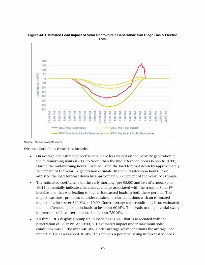
80

Figure 44: Estimated Load Impact of Solar Photovoltaic Generation: San Diego Gas & Electric Total


Observations about these data include:

• On average, the estimated coefficients place less weight on the Solar PV generation in

the mid-morning hours (08:00 to Noon) than the mid-afternoon hours (Noon to 16:00).

During the mid-morning hours, Itron adjusted the load forecast down by approximately

50 percent of the Solar PV generation estimate. In the mid-afternoon hours, Itron

adjusted the load forecast down by approximately 77 percent of the Solar PV estimate.

• The estimated coefficients on the early morning (pre 08:00) and late afternoon (post

16:45) potentially indicate a behavioral change associated with the trend in Solar PV

installations that was leading to higher forecasted loads in both these periods. This

impact was most pronounced under maximum solar conditions with an estimated

impact of a little over 840 MW at 19:00. Under average solar conditions, Itron estimated

the late afternoon pick up in loads to be about 60 MW. This leads to the potential swing

in forecasts of late afternoon loads of about 780 MW.

• All three IOUs display a bump up in loads post 16:45 that is associated with the

penetration of Solar PV. At 19:00, SCE estimated impact under maximum solar

conditions was a little over 540 MW. Under average solar conditions the average load

impact at 19:00 was about 30 MW. This implies a potential swing in forecasted loads

81

between a maximum solar condition day and an average solar condition day of about

510 MW.

• At 19:00, PG&E estimated impact under maximum solar conditions was a little over 170

MW. Under average solar conditions, the average load impact at 19:00 was about 15 MW.

This implies a potential swing in forecasted loads between a maximum solar condition

day and an average solar condition day of about 160 MW.

• At 19:00, PG&E estimated impact under maximum solar conditions was a little over 120

MW. Under average solar conditions, the average load impact at 19:00 was about 5 MW.

This implies a potential swing in forecasted loads between a maximum solar condition

day and an average solar condition day of about 115 MW.

• In the early morning hours (pre-08:00) there was a similar forecasted rise in loads

associated with penetration in Solar PV. This impact was most pronounced with PG&E

with an estimated load impact of about 400 MW under maximum solar conditions. Itron

estimated the impact on SCE early morning hours to be a little over 200 MW under

maximum solar conditions. SDG&E does not have this type impact.

The results highlight another operational challenge in that the impact of Solar PV generation

varies not only in magnitude across the three IOUs, but also the timing of the maximum impact.

This reflects the fact that the time at which the sun is at its zenith depends on where the loads

are located. The geographic distance between the PG&E, SCE and SDG&E is sufficient to lead to

differences in when the solar generation impact will be at its highest. This in turn implies the

timing and order of magnitude of the late afternoon ramp-up in loads associated with a

ramping down of Solar PV generation will vary across the year and across the three IOU loads.

The analysis of the statistically adjusted load impact of Solar PV generation reflects the

challenge with the Model Direct approach. In all cases, one rejects the engineering-based a

priori value for the estimated coefficient on the Solar PV generation variable of -1.0. This does

not mean that one (1) MW of Solar PV generation does not reduce load by one (1) MW. Rather

models of measured load are challenged in isolating the impact of Solar PV generation from

other potentially highly correlated factors that drive weather sensitive loads. Further, the

estimated coefficients on the Solar PV generation variables will be skewed to account for these

behavioral changes to the extent penetration of Solar PV leads to behavioral changes whereby

people are taking advantage of “free” electricity. While it would be nice to have all of the

estimated coefficients with a value close to -1.0, the goal was to improve the load forecast. To

that end, the statistical models optimize the coefficient values to reduce load forecast errors.

By not imposing a priori constraints on the estimated coefficients, the models are able to

capture the net impact of a growing penetration of Solar PV.

82

Chapter 5: Forecasting Valuation and Framework Analysis


The goals of this research task are 1) to analyze costs to determine the value of utilizing

improved PV solar forecasts to utilities, grid operators, and California investor-owned utility

(IOU) ratepayers; and 2) to leverage the improved forecasts and data from the earlier tasks to

help utilities and the California ISO better integrate increasing amounts of renewables on the

grid with lower costs. This section discusses these goals.

The valuation of any increased accuracy of the net load forecast from an alternative forecast

method over the California Independent System Operator (California ISO) baseline forecast is

dependent on the timeframe of the forecast. In the case of the research14 demonstrated in

Task 4 that this cost analysis applies to, the timeframe is the day-ahead and day-of. This is

important because it determines what costs are relevant in determining the value of an

alternative forecast method.

Valuation of Alternative Forecast Method

The fundamental premise with using short term market pricing is that the forecast (Baseline or

Alternative) used doesn’t matter because at the end of the day, the actual electricity consumed

is the same. Therefore, the valuation is dependent on three components; 1) the cost of

reserving resources the day-ahead to supply the forecasted load, 2) the cost of making day-of

adjustments to the forecasted load, and 3) the cost of making final adjustments to cover the

difference between the forecasted load and the actual load.

The first element of the valuation is the calculation of the cost to reserve supply the day ahead

based on each of the respective day ahead forecasts. Itron used the day ahead market (DAM)

locational marginal price (LMP) to value the differences between the Baseline and Alternative

forecasts. The size of these forecast differences was relatively small compared to the total

forecasted net load. It is reasonable to use DAM LMP prices to value the forecast differences

because the total amount of energy associated with the differences in the forecasts can

reasonably be purchased in the DAM.

The second element of the valuation is the calculation of the cost to adjust the reserved supply

in the day-of based on the day-of forecasts. The California ISO Trues-up the forecast in the day-

of market. These are purchased in the hour ahead scheduling process (HASP) at HASP LMP

14 Monforte, Dr. Frank A.; Fordham, Christine; Blanco, Jennifer; Barsun, Stephan (Itron, Inc.) Kankiewicz, Adam; Norris,

Ben (Clean Power Research). 2016. Improving Short-Term Load Forecasts by Incorporating Solar PV Generation. California Energy Commission.

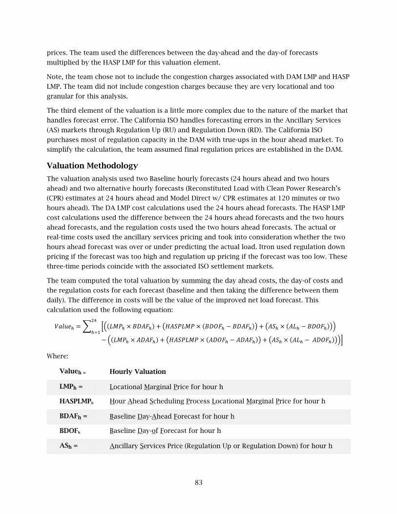
83

prices. The team used the differences between the day-ahead and the day-of forecasts

multiplied by the HASP LMP for this valuation element.

Note, the team chose not to include the congestion charges associated with DAM LMP and HASP

LMP. The team did not include congestion charges because they are very locational and too

granular for this analysis.

The third element of the valuation is a little more complex due to the nature of the market that

handles forecast error. The California ISO handles forecasting errors in the Ancillary Services

(AS) markets through Regulation Up (RU) and Regulation Down (RD). The California ISO

purchases most of regulation capacity in the DAM with true-ups in the hour ahead market. To

simplify the calculation, the team assumed final regulation prices are established in the DAM.

Valuation Methodology

The valuation analysis used two Baseline hourly forecasts (24 hours ahead and two hours

ahead) and two alternative hourly forecasts (Reconstituted Load with Clean Power Research’s

(CPR) estimates at 24 hours ahead and Model Direct w/ CPR estimates at 120 minutes or two

hours ahead). The DA LMP cost calculations used the 24 hours ahead forecasts. The HASP LMP

cost calculations used the difference between the 24 hours ahead forecasts and the two hours

ahead forecasts, and the regulation costs used the two hours ahead forecasts. The actual or

real-time costs used the ancillary services pricing and took into consideration whether the two

hours ahead forecast was over or under predicting the actual load. Itron used regulation down

pricing if the forecast was too high and regulation up pricing if the forecast was too low. These

three-time periods coincide with the associated ISO settlement markets.

The team computed the total valuation by summing the day ahead costs, the day-of costs and

the regulation costs for each forecast (baseline and then taking the difference between them

daily). The difference in costs will be the value of the improved net load forecast. This

calculation used the following equation:

𝑉𝑎𝑙𝑢𝑒ℎ = ∑ [((𝐿𝑀𝑃ℎ × 𝐵𝐷𝐴𝐹ℎ) + (𝐻𝐴𝑆𝑃𝐿𝑀𝑃 × (𝐵𝐷𝑂𝐹ℎ − 𝐵𝐷𝐴𝐹ℎ)) + (𝐴𝑆ℎ × (𝐴𝐿ℎ − 𝐵𝐷𝑂𝐹ℎ)))24

ℎ=1

− ((𝐿𝑀𝑃ℎ × 𝐴𝐷𝐴𝐹ℎ) + (𝐻𝐴𝑆𝑃𝐿𝑀𝑃 × (𝐴𝐷𝑂𝐹ℎ − 𝐴𝐷𝐴𝐹ℎ)) + (𝐴𝑆ℎ × (𝐴𝐿ℎ − 𝐴𝐷𝑂𝐹ℎ)))]

Where:

Valueh = Hourly Valuation

LMPh = Locational Marginal Price for hour h

HASPLMPh Hour Ahead Scheduling Process Locational Marginal Price for hour h

BDAFh = Baseline Day-Ahead Forecast for hour h

BDOFh Baseline Day-of Forecast for hour h

ASh = Ancillary Services Price (Regulation Up or Regulation Down) for hour h

84

ALh = Actual Load for hour h

ADAFh = Alternative Day-Ahead Forecast for hour h

ADOFh Alternative Day-of Forecast for hour h

The project team evaluated each of the five California ISO subzones (PG&E Bay Area, PG&E Non-

Bay Area, SCE Coastal, SCE Inland, and SDG&E) and for the California ISO. The date range for

conducting the valuation analysis goes from January 1, 2012 through June 8, 2015.

To better understand the influence of market prices on the forecast valuation, the following

sub-sections summarize them and their associated seasonality and volatility.

Locational Marginal Prices

The DAM provides the LMP for all nodes managed by the California ISO. These nodal LMPs have

three components. The first is the energy component, the second is the congestion charge for

that location, and the third is associated with line loses. The energy component is the same for

all nodes. Only the energy component for the valuation analysis was used.

Figure 45 and Figure 46 show the range of hourly LMPs for the summer 2014 and the spring

2015 respectively using box-and-whisker plots. Box and whisker plots illustrate the degree of

dispersion, skewness and general variability of the data. There is a box representing each hour

of all days in the period. The line in the center of each greyed box is the median price value and

the ends of the box are the interquartile value (IQR)15 in distance from the center line. The

spread of one IQR on either side of the center line represents the spread where 50 percent of

the values lie. The lines or whiskers further outside the box on either end are 1.5 times the IQR.

During the summer season, the LMP profile looks much like the system load profile with the

greatest variation in price occurring at the system peak hours. During the other seasons, the

average LMPs during the mid-day hours are relatively flat, but the day to day prices range

widely for a given hour.

15 See: https://en.wikipedia.org/wiki/Interquartile_range

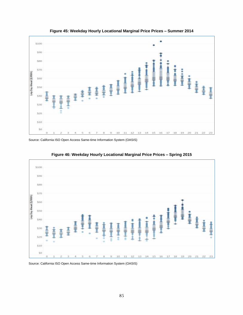
85

Figure 45: Weekday Hourly Locational Marginal Price Prices – Summer 2014

Source: California ISO Open Access Same-time Information System (OASIS)

Figure 46: Weekday Hourly Locational Marginal Price Prices – Spring 2015


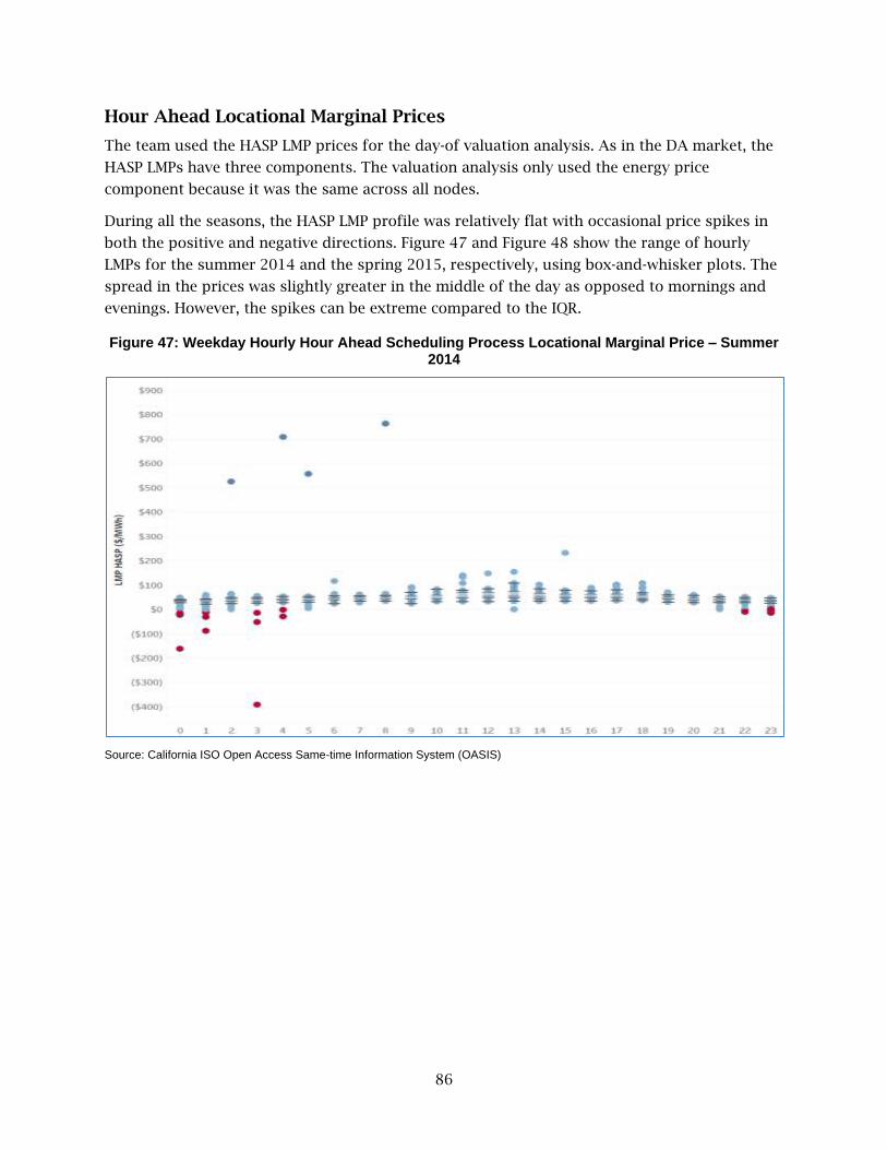
86

Hour Ahead Locational Marginal Prices

The team used the HASP LMP prices for the day-of valuation analysis. As in the DA market, the

HASP LMPs have three components. The valuation analysis only used the energy price

component because it was the same across all nodes.

During all the seasons, the HASP LMP profile was relatively flat with occasional price spikes in

both the positive and negative directions. Figure 47 and Figure 48 show the range of hourly

LMPs for the summer 2014 and the spring 2015, respectively, using box-and-whisker plots. The

spread in the prices was slightly greater in the middle of the day as opposed to mornings and

evenings. However, the spikes can be extreme compared to the IQR.

Figure 47: Weekday Hourly Hour Ahead Scheduling Process Locational Marginal Price – Summer 2014


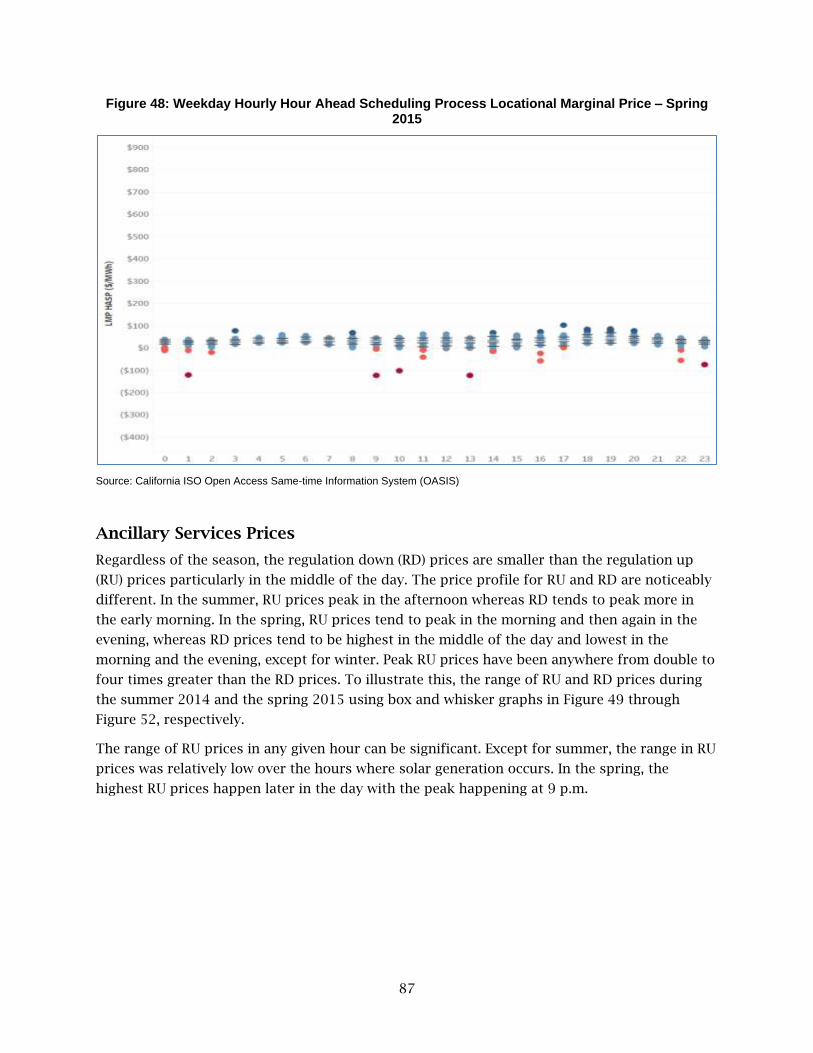
87

Figure 48: Weekday Hourly Hour Ahead Scheduling Process Locational Marginal Price – Spring 2015


Ancillary Services Prices

Regardless of the season, the regulation down (RD) prices are smaller than the regulation up

(RU) prices particularly in the middle of the day. The price profile for RU and RD are noticeably

different. In the summer, RU prices peak in the afternoon whereas RD tends to peak more in

the early morning. In the spring, RU prices tend to peak in the morning and then again in the

evening, whereas RD prices tend to be highest in the middle of the day and lowest in the

morning and the evening, except for winter. Peak RU prices have been anywhere from double to

four times greater than the RD prices. To illustrate this, the range of RU and RD prices during

the summer 2014 and the spring 2015 using box and whisker graphs in Figure 49 through

Figure 52, respectively.

The range of RU prices in any given hour can be significant. Except for summer, the range in RU

prices was relatively low over the hours where solar generation occurs. In the spring, the

highest RU prices happen later in the day with the peak happening at 9 p.m.

88

Figure 49: Weekday Regulation Up Prices – Summer 2014


Figure 50: Weekday Regulation Down Prices – Summer 2014


89

Figure 51: Weekday Regulation Up Prices – Spring 2015


Figure 52: Weekday Regulation Down Prices – Spring 2015


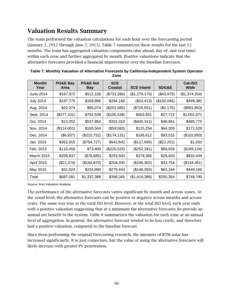
90

Valuation Results Summary

The team performed the valuation calculations for each hour over the forecasting period

(January 1, 2012 through June 7, 2015). Table 7 summarizes these results for the last 12

months. The team has aggregated valuation components (day-ahead, day-of, and real-time)

within each zone and further aggregated by month. Positive valuations indicate that the

alternative forecasts provided a financial improvement over the baseline forecasts.

Table 7: Monthly Valuation of Alternative Forecasts by California-Independent System Operator Zone

Month/ Year

PG&E Bay Area

PG&E Not Bay

SCE Coastal SCE Inland SDG&E

Cal-ISO Wide

June 2014 $167,972 $512,106 ($731,286) ($1,279,170) ($43,975) ($1,374,354)

July 2014 $197,775 $169,896 $294,169 ($10,413) ($152,045) $499,382

Aug. 2014 $22,374 $65,074 ($251,585) ($725,651) ($2,175) ($891,963)

Sept. 2014 ($277,101) $792,538 ($105,638) $563,551 $27,722 $1,001,071

Oct. 2014 $13,252 $537,854 $331,019 ($445,311) $48,961 $485,775

Nov. 2014 ($114,001) $165,564 ($59,593) $115,254 $64,305 $171,529

Dec. 2014 ($6,937) ($210,752) ($174,131) $195,612 $93,515 ($102,693)

Jan. 2015 $352,915 ($754,727) $542,642 ($117,595) ($22,201) $1,033

Feb. 2015 $110,455 $73,400 ($220,525) ($252,391) $99,926 ($189,134)

March 2015 $209,837 ($78,685) $293,500 $379,385 $29,403 $833,439

April 2015 ($21,374) ($164,870) $204,330 ($196,302) $43,754 ($134,461)

May 2015 $31,924 $224,990 $275,443 ($146,355) $63,164 $449,166

Total $687,091 $1,332,388 $398,345 ($1,919,386) $250,354 $748,790

Source: Itron Valuation Analysis

The performance of the alternative forecasts varies significant by month and across zones. At

the zonal level, the alternative forecasts can be positive or negative across months and across

years. The same was true at the total ISO level. However, at the total ISO level, each year ends

with a positive valuation suggesting that at a minimum the alternative forecasts do provide an

annual net benefit to the system. Table 8 summarizes the valuation for each zone at an annual

level of aggregation. In general, the alternative forecast tended to be less costly, and therefore

had a positive valuation, compared to the baseline forecast.

Since Itron performing the original forecasting research, the amounts of BTM solar has

increased significantly. It is just conjecture, but the value of using the alternative forecasts will

likely increase with greater PV penetration.

91

Table 8: Annual Valuation of Alternative Forecasts by California Independent System Operator Zone

Year

PG&E Bay Area

PG&E Not Bay

SCE Coastal

SCE Inland SDG&E Cal-ISO

Wide

2012 $1,393,854 ($1,659,008) ($2,973,766) $3,290,775 $55,386 $107,241

2013 $2,132,599 $4,059,191 $1,862,615 ($1,746,753) $735,379 $7,043,032

2014 $1,423,229 $1,565,879 ($3,081,437) $2,294,784 ($691,664) $1,510,790

2015 $689,004 ($762,631) $919,519 ($441,993) $171,932 $575,832

Total $5,638,686 $3,203,431 ($3,273,069) $3,396,814 $271,032 $9,236,894


Costing Period Components

To get a better picture of which of the costing period components (day-ahead, hour-ahead, and

regulation) are more significant to the overall valuation, they are shown in Table 9 and Table 10

by baseline and alternative forecast respectively for the PG&E Bay Area zone. The day-ahead

component was by far the largest cost component followed by the hour-ahead and then the

regulation cost components. This same pattern of cost magnitude exists across all the

forecasting zones.

Table 9: Pacific Gas & Electric Bay Area Baseline Forecast Costing Period Components

Month & Year Day-Ahead-Base

Cost Hour-Ahead Base

Cost Regulation Base

Cost Total Base Cost

June 2014 $148,625,381 $2,811,642 $287,258 $151,724,282

July 2014 $184,272,895 $2,999,219 $249,384 $187,521,498

August 2014 $178,833,076 $3,187,751 $225,596 $182,246,422

September 2014

$177,941,290 $4,747,989 $234,721 $182,924,001

October 2014 $122,008,465 $4,175,888 $242,596 $126,426,949

November 2014

$53,108,720 $1,598,932 $81,544 $54,789,195

December 2014

$125,946,041 $3,731,631 $212,649 $129,890,320

January 2015 $122,415,932 $1,368,015 $187,335 $123,971,282

February 2015 $101,194,214 $3,405,808 $152,302 $104,752,324

March 2015 $112,263,892 $363,099 $134,047 $112,761,038

April 2015 $95,718,062 $2,160,373 $163,304 $98,041,739

May 2015 $100,938,058 $680,025 $167,625 $101,785,708

Grand Total $1,523,266,023 $31,230,374 $2,338,361 $1,556,834,758


92

Table 10: Pacific Gas & Electric Bay Area Alternative Forecast Costing Period Components

Month & Year Day-Ahead

Alternative Cost Hour-Ahead

Alternative Cost Regulation

Alternative Cost Total Alternative

Cost

June 2014 $149,006,811 $2,270,814 $278,684 $151,556,310

July 2014 $183,473,775 $3,601,809 $248,139 $187,323,723

August 2014 $178,419,254 $3,582,755 $222,039 $182,224,048

September 2014

$179,929,939 $3,039,088 $232,075 $183,201,102

October 2014 $122,892,932 $3,276,006 $244,760 $126,413,697

November 2014

$54,052,230 $765,608 $85,359 $54,903,197

December 2014

$125,755,596 $3,937,017 $204,645 $129,897,257

January 2015 $120,771,392 $2,671,963 $175,011 $123,618,367

February 2015 $102,596,993 $1,902,449 $142,427 $104,641,869

March 2015 $111,866,415 $556,150 $128,636 $112,551,201

April 2015 $95,962,370 $1,941,639 $159,103 $98,063,113

May 2015 $100,356,784 $1,236,519 $160,481 $101,753,784

Grand Total $1,525,084,492 $28,781,817 $2,281,359 $1,556,147,667


It would appear from these cost summaries that the day-ahead forecast costs are the most

important until one computes the valuation for each of the individual period components.

Table 11 shows the difference between baseline and alternative costs (that is valuation) for each

period component for the last 12 complete months of alternative forecasts. Both the day-ahead

and the hour-ahead valuation components are of similar absolute magnitude. The difference in

regulation costs, however, are much smaller and therefore less significant. Even with the

California ISO’s change in regulation procurement beginning in February of 2016, the impact of

regulation on valuation was still small. This examination of the period components may provide

some guidance in developing a forecasting framework.

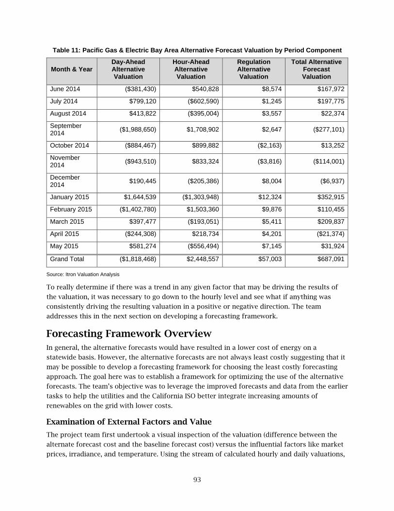
93

Table 11: Pacific Gas & Electric Bay Area Alternative Forecast Valuation by Period Component

Month & Year Day-Ahead Alternative Valuation

Hour-Ahead Alternative Valuation

Regulation Alternative Valuation

Total Alternative Forecast Valuation

June 2014 ($381,430) $540,828 $8,574 $167,972

July 2014 $799,120 ($602,590) $1,245 $197,775

August 2014 $413,822 ($395,004) $3,557 $22,374

September 2014

($1,988,650) $1,708,902 $2,647 ($277,101)

October 2014 ($884,467) $899,882 ($2,163) $13,252

November 2014

($943,510) $833,324 ($3,816) ($114,001)

December 2014

$190,445 ($205,386) $8,004 ($6,937)

January 2015 $1,644,539 ($1,303,948) $12,324 $352,915

February 2015 ($1,402,780) $1,503,360 $9,876 $110,455

March 2015 $397,477 ($193,051) $5,411 $209,837

April 2015 ($244,308) $218,734 $4,201 ($21,374)

May 2015 $581,274 ($556,494) $7,145 $31,924

Grand Total ($1,818,468) $2,448,557 $57,003 $687,091


To really determine if there was a trend in any given factor that may be driving the results of

the valuation, it was necessary to go down to the hourly level and see what if anything was

consistently driving the resulting valuation in a positive or negative direction. The team

addresses this in the next section on developing a forecasting framework.

Forecasting Framework Overview

In general, the alternative forecasts would have resulted in a lower cost of energy on a

statewide basis. However, the alternative forecasts are not always least costly suggesting that it

may be possible to develop a forecasting framework for choosing the least costly forecasting

approach. The goal here was to establish a framework for optimizing the use of the alternative

forecasts. The team’s objective was to leverage the improved forecasts and data from the earlier

tasks to help the utilities and the California ISO better integrate increasing amounts of

renewables on the grid with lower costs.

Examination of External Factors and Value

The project team first undertook a visual inspection of the valuation (difference between the

alternate forecast cost and the baseline forecast cost) versus the influential factors like market

prices, irradiance, and temperature. Using the stream of calculated hourly and daily valuations,

94

the team examined the alternative forecasts under various conditions that might indicate when

they provide the most value.

There are many factors at work that influence the valuation and identifying a simple

forecasting framework may not be possible. To explore this visually, project team first

developed several plots of the valuation versus influential factors. The influential factors

examined included market prices, irradiance, and temperature. Figure 53 shows scatter plots of

the calculated hourly valuations and how they relate to the various potentially influential

factors (LMP, HASP LMP, RU, RD, irradiance, and temperature.)

Figure 53: Pacific Gas & Electric Bay Area – Alternative Forecasts Valuation vs. Prices, Irradiance and Temperature


Figure 53 also examines several potential key indicators against these influential factors. These

include the day ahead alternative forecast errors (the difference between the day ahead forecast

and the actual load), the day-of alternative forecast errors (the difference between the day-of

forecast and the actual load), and the difference between the day ahead and day-of alternative

forecasts. In all cases, there were no clear or consistent correlations between influential factors

and key indicators and the alternative forecast valuations. For example, one would think

irradiance16 would be an influential factor in explaining when the alternative forecast was less

costly than the baseline forecast. If irradiance was a reliably predictor, something like a slanted

line running through the plots could be seen. When the team looked at the irradiance column of

16 The power per unit area received from the sun.

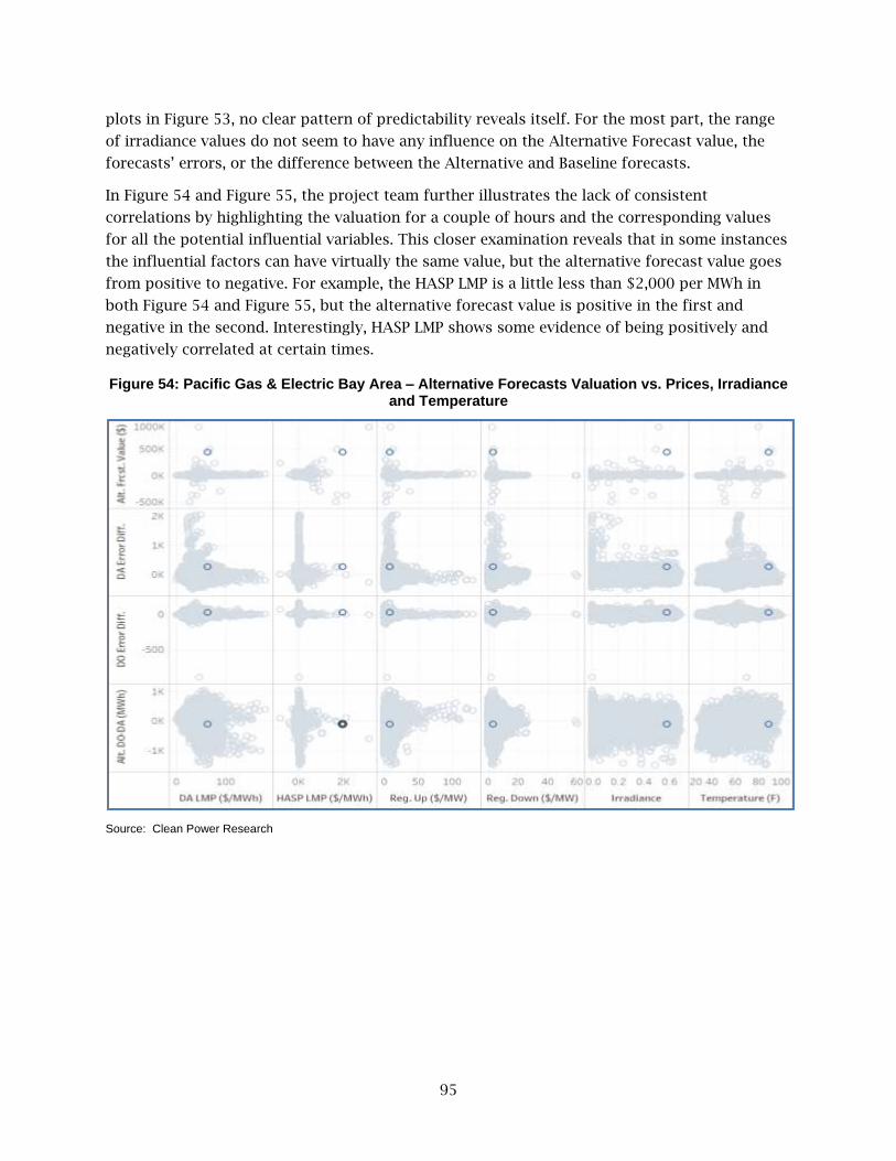
95

plots in Figure 53, no clear pattern of predictability reveals itself. For the most part, the range

of irradiance values do not seem to have any influence on the Alternative Forecast value, the

forecasts’ errors, or the difference between the Alternative and Baseline forecasts.

In Figure 54 and Figure 55, the project team further illustrates the lack of consistent

correlations by highlighting the valuation for a couple of hours and the corresponding values

for all the potential influential variables. This closer examination reveals that in some instances

the influential factors can have virtually the same value, but the alternative forecast value goes

from positive to negative. For example, the HASP LMP is a little less than $2,000 per MWh in

both Figure 54 and Figure 55, but the alternative forecast value is positive in the first and

negative in the second. Interestingly, HASP LMP shows some evidence of being positively and

negatively correlated at certain times.

Figure 54: Pacific Gas & Electric Bay Area – Alternative Forecasts Valuation vs. Prices, Irradiance and Temperature


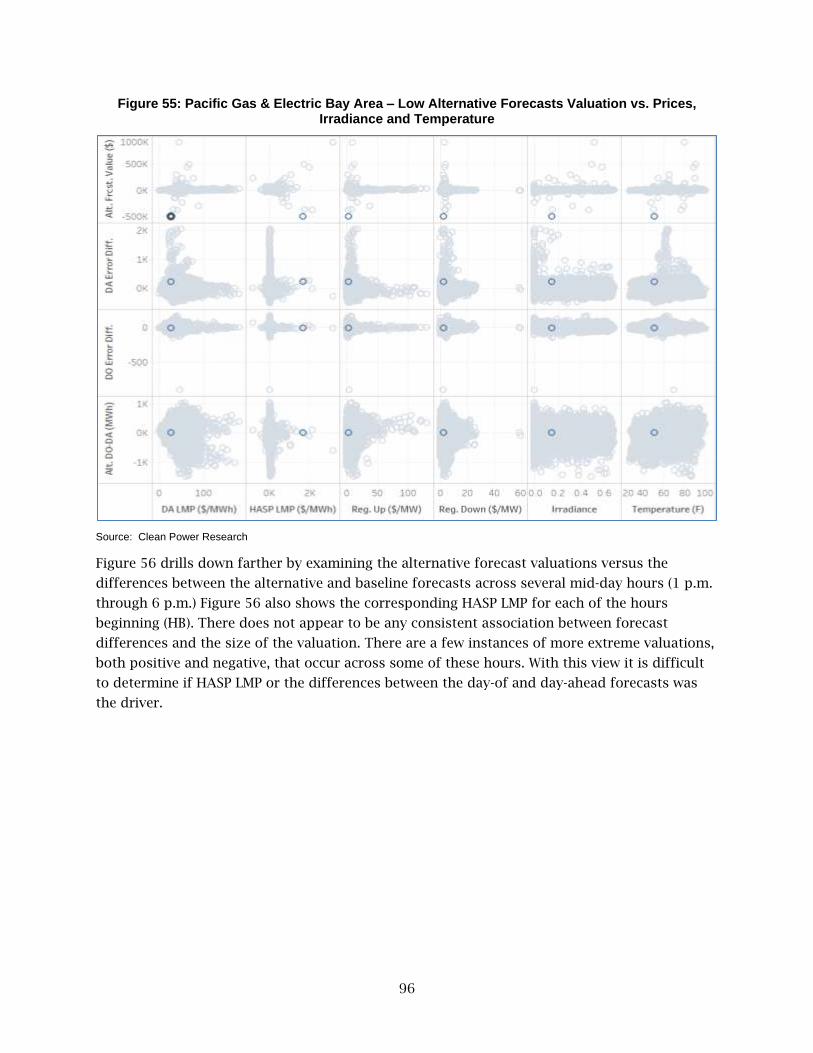
96

Figure 55: Pacific Gas & Electric Bay Area – Low Alternative Forecasts Valuation vs. Prices, Irradiance and Temperature


Figure 56 drills down farther by examining the alternative forecast valuations versus the

differences between the alternative and baseline forecasts across several mid-day hours (1 p.m.

through 6 p.m.) Figure 56 also shows the corresponding HASP LMP for each of the hours

beginning (HB). There does not appear to be any consistent association between forecast

differences and the size of the valuation. There are a few instances of more extreme valuations,

both positive and negative, that occur across some of these hours. With this view it is difficult

to determine if HASP LMP or the differences between the day-of and day-ahead forecasts was

the driver.

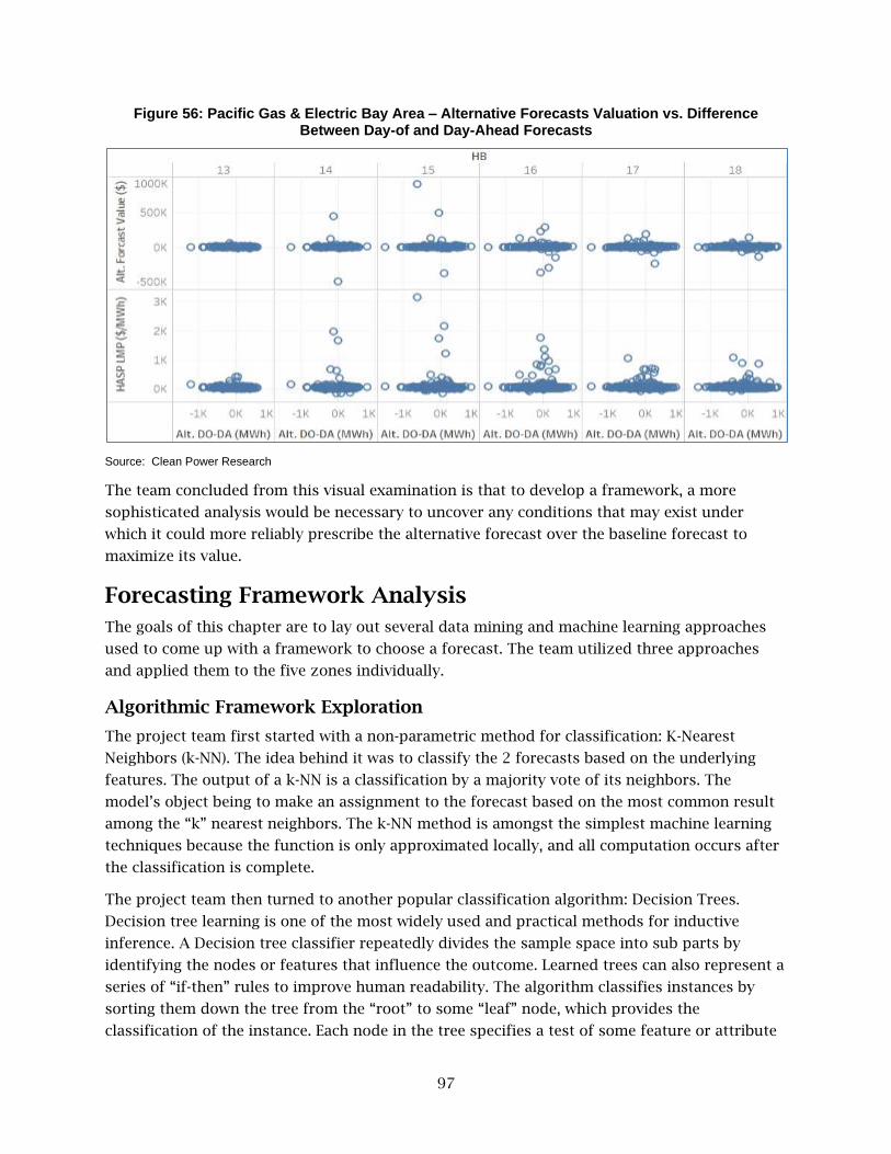
97

Figure 56: Pacific Gas & Electric Bay Area – Alternative Forecasts Valuation vs. Difference Between Day-of and Day-Ahead Forecasts


The team concluded from this visual examination is that to develop a framework, a more

sophisticated analysis would be necessary to uncover any conditions that may exist under

which it could more reliably prescribe the alternative forecast over the baseline forecast to

maximize its value.

Forecasting Framework Analysis

The goals of this chapter are to lay out several data mining and machine learning approaches

used to come up with a framework to choose a forecast. The team utilized three approaches

and applied them to the five zones individually.

Algorithmic Framework Exploration

The project team first started with a non-parametric method for classification: K-Nearest

Neighbors (k-NN). The idea behind it was to classify the 2 forecasts based on the underlying

features. The output of a k-NN is a classification by a majority vote of its neighbors. The

model’s object being to make an assignment to the forecast based on the most common result

among the “k” nearest neighbors. The k-NN method is amongst the simplest machine learning

techniques because the function is only approximated locally, and all computation occurs after

the classification is complete.

The project team then turned to another popular classification algorithm: Decision Trees.

Decision tree learning is one of the most widely used and practical methods for inductive

inference. A Decision tree classifier repeatedly divides the sample space into sub parts by

identifying the nodes or features that influence the outcome. Learned trees can also represent a

series of “if-then” rules to improve human readability. The algorithm classifies instances by

sorting them down the tree from the “root” to some “leaf” node, which provides the

classification of the instance. Each node in the tree specifies a test of some feature or attribute

98

of the instance, and each branch descending from the node corresponds to one of the possible

values of the attribute.17

Lastly, the project team developed a Random Forest model. Random Forests are an ensemble

learning method for classification that operate by constructing a multitude of decision trees at

training time and outputting the forecast that is the mode (most common) of both the

forecasts. They are a much more sophisticated and complex machine learning algorithm than

the decision trees and correct for the overfitting bias in the decision trees. The Random Forest

models grow out decision trees much deeper (more nodes) than the decision stumps shown

above (from the decision tree algorithm), in fact the default behavior is to grow out each tree as

far as possible (recall that to simply matters, the decision tree was reduced to one node). There

is a direct relationship between the number of trees in the forest and the results it can get: the

larger the number of decision trees, the more accurate the result.

Framework Analysis Summary

Summary of Results

Using these Machine Learning approaches, the researchers calculated the cost to purchase

energy in the California ISO markets associated with each forecast. Table 12 shows the cost

associated with the forecast chosen based on each of these Machine Learning models

developed. While the research team believes there is merit in the Machine Learning approaches

taken to understand the conditions under which a forecast should be chosen, the underlying

data was very noisy and depended on too many features which makes it difficult to fit simple

and interpretable Machine Learning models.

17 http://www.cs.princeton.edu/courses/archive/spr07/cos424/papers/mitchell-dectrees.pdf

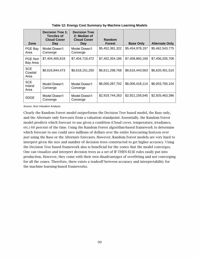
99

Table 12: Energy Cost Summary by Machine Learning Models

Zone

Decision Tree 1: Terciles of

Cloud Cover Day

Decision Tree 2: Median of Cloud Cover

Day Random Forest Base Only Alternate Only

PGE Bay Area

Model Doesn’t Converge


$5,452,381,322

$5,454,978,197

$5,462,543,775

PGE Non Bay Area

$7,404,465,618

$7,404,718,472

$7,402,354,186

$7,408,860,169

$7,406,205,706

SCE Coastal Area

$6,616,844,473

$6,618,151,250

$6,611,298,768

$6,616,443,563

$6,620,451,510

SCE Inland Area



$6,000,287,702

$6,006,418,114

$6,003,756,104

SDGE Model Doesn’t Converge


$2,919,744,263

$2,921,159,545

$2,925,463,396


Clearly the Random Forest model outperforms the Decision Tree based model, the Base only,

and the Alternate only forecasts from a valuation standpoint. Essentially, the Random Forest

model predicts which forecast to use given a condition (Cloud cover, temperature, irradiance,

etc.) 60 percent of the time. Using the Random Forest algorithm-based framework to determine

which forecast to use could save millions of dollars over the entire forecasting horizon over

just using the Base or the Alternate forecasts. However, Random Forest models are very hard to

interpret given the size and number of decision trees constructed to get higher accuracy. Using

the Decision Tree based framework also is beneficial for the zones that the model converges.

One can visualize and interpret decision trees as a set of IF-THEN-ELSE rules easily put into

production. However, they come with their own disadvantages of overfitting and not converging

for all the zones. Therefore, there exists a tradeoff between accuracy and interpretability for

the machine learning-based frameworks.

100

Chapter 6: Conclusions and Recommendations


Conclusions

The use of real time data for forecasting plant output shows promise, and warrants further

pursuit. Plant availability would be of particular interest; however, the inclusion of security

protocols would require close coordination with California ISO and possibly the individual plant

operators.

Recommendations

A test of CSP forecasting may also prove valuable. One could develop Forecasts for CSP

resources without storage (the simplest case), but one could also develop methods for storage

dispatch using defined objectives, such as revenue maximization.


Conclusions

The research team has shown many of the methods to improve forecasting which have been

implemented in software (or are ready for implementation). These relate to module

degradation, fleet-level availability, improving the inverter power curve, ensemble methods, and

dynamic fleet capacity tracking. Some insights gained from this work suggests additional

investigation may yield further forecast accuracy benefits.

Recommendations

The accuracy of assessing system specifications by inference requires some additional study, as

does assessing the importance of shading, and the lack of shading data from the original site

installation. These could be topics for future research.


Conclusions

This study set out to determine if there was a way of improving the load forecast accuracy of

the California ISO’s existing load forecast models by incorporating forecasts of solar PV

generation. The research team presents three alternative modeling approaches. These

approaches were subject to a forecast simulation using solar PV generation driven by hourly

cloud cover for a handful of weather stations and solar PV generation estimates developed by

101

CPR using a detailed database of solar PV installations combined with satellite imagery. The

conclusions from this study include the following outlined below.

• Not adjusting the California ISO baseline forecast models will only lead to further

erosion of forecast accuracy and a greater dispersion of forecast errors.

• For forecast horizons of 15 minutes ahead to four hours ahead, the Model Direct

approach, when combined with the CPR estimates of solar generation, provides

improved forecast accuracy and reduced forecast error dispersion over the baseline load

forecast model. This finding indicates the benefit of relaxing the assumption that 1 MW

of BTM solar PV generation leads to a 1 MW reduction in measured load which is a key

assumption of both the Reconstituted Load and Error Correction approaches. These

approaches assume both: (1) no underlying behavioral changes take place as a result of

the installation of solar PV and (2) the BTM solar PV estimates are correct. In contrast,

the Direct Model through the process of model estimation is able to capture the

influence of behavioral changes on the estimated BTM solar PV generation impact, as

well as make statistical adjustments for incorrect BTM solar PV estimates. This finding

also provides evidence of the benefit of CPR’s more granular approach to developing

BTM solar PV generation over the use of a cloud cover driven forecast for a handful of

weather stations.

• For longer term forecast horizons of six hours ahead to 24 hours ahead, the

Reconstituted Load approach, combined with the CPR estimates of solar generation,

provide improvements in both forecast accuracy and reduced forecast error dispersion

over the baseline load forecast model.

• This suggests a hybrid forecast framework that leverages the forecasts from the Model

Direct approach for forecast horizons of 15 minutes ahead to four hours ahead and

then switches to the Reconstituted Load approach for forecasts horizons of fours-ahead

and longer.

• Hourly cloud cover driven estimates of solar generation can provide benefit over doing

nothing, however the detail bottom-up approach implemented by CPR yields superior

results.

• The fact the results vary by season and cloud cover conditions suggest introducing

seasonal and cloud cover interaction terms in the Model Direct approach. This would

allow the load impact of the solar generation variable to vary by season and cloud cover

conditions.

• Other interaction terms including Day-of-the-Week and possibly temperature conditions

may also prove useful in improving the accuracy of the Model Direct approach.

• The estimated coefficients of the Model Direct models provide evidence for the potential

of long-run behavioral changes associated with the increased penetration of solar PV. If

true, then the Error Correction and Reconstituted Load approaches will lose forecast

skill over time as the assumption that the coefficient on the solar PV generation variable

should be -1.0 becomes invalid.

102

Recommendations

With further research the extent to which penetration of solar PV is leading to behavioral

changes can be determined. As part of the upcoming California Solar Initiative Final Impact

Evaluations, Itron will be starting to investigate this question. If the answer is yes, then the load

forecasting problem will only become more complicated with further penetration of solar PV

combined with growth in electric vehicle charging, on-site electricity storage, and integration

into emerging models such as microgrids.

Forecast Valuation & Framework Analysis

Conclusions

Calculating the value of the alternative forecasting approach that incorporates solar forecasts,

requires using a valuation method that uses appropriate costs. Short-term load forecast

estimates do not affect longer-term capital investments. Therefore, the research team believes

that it is best to calculate the proper costs using the publicly available market prices used for

settlement purposes by the California ISO in its day-ahead, hour-ahead and regulation markets.

The value of the alternative forecasts is in general positive, suggesting that they perform better

financially than the California ISO baseline forecasts. Not all periods show this to be the case

and it varies across all zones examined as well. It may be possible to develop a forecasting

framework that specifies when to use either the alternative or the baseline forecasts thereby

optimizing the value associated with the alternative forecasts.

Even though there is an economic value in using these machine learning approaches, the

models are very difficult to interpret and operationalize in real conditions. At the total ISO

level, each year ends with a positive valuation suggesting that, at a minimum, the alternative

forecasts do provide an annual net benefit to the system if used all the time.

Recommendations

To improve the Machine Learning approaches, there needs to be more research in three areas.

• Influential factors

• Increasing the size of the training dataset

• Other machine learning algorithms

• Testing with recent alternative forecasting model results

First, there must be research to identify the best influential factors to use. The team limited this

research to just those factors that were available to the alternative forecast method

development. There may be better factors that were not available for this research. For

example, because the zones cover large geographic areas, it may be better to use irradiance

values averaged across a number of monitoring locations.

Second, increasing the size of the training dataset could increase the prediction accuracy. In

most studies of classification, there is a rising accuracy curve with respect to the size of the

103

training dataset. Therefore, increasing the forecast horizon to include more years would lead to

a bigger training dataset that could ultimately increase the prediction accuracy.

Third, research into other types of Machine Learning algorithms must be done.18 This research

only attempted three types. There are numerous other algorithms worthy of consideration.

Some of these include Linear Discriminant Analysis, Naïve Bayes, Learning Vector Quantization,

Support Vector Machines, and Boosting. Some of these models may perform better and may be

easier to operationalize. This would improve the chances stakeholders would accept and use

them.

Lastly, the research team used the alternative forecasts developed for a forecast horizon that

may not be relevant to today’s conditions. BTM solar has grown substantially since the

beginning of 2015. Examination of the impacts of this on the alternative forecasts’ accuracy and

ability to better perform than the California ISO’s baseline forecasts is warranted. In addition,

Itron has made improvements to its body of knowledge concerning forecasting models that

incorporate BTM solar. These improved models should be considered.as replacements for those

developed during this project.

18 https://machinelearningmastery.com/a-tour-of-machine-learning-algorithms/.

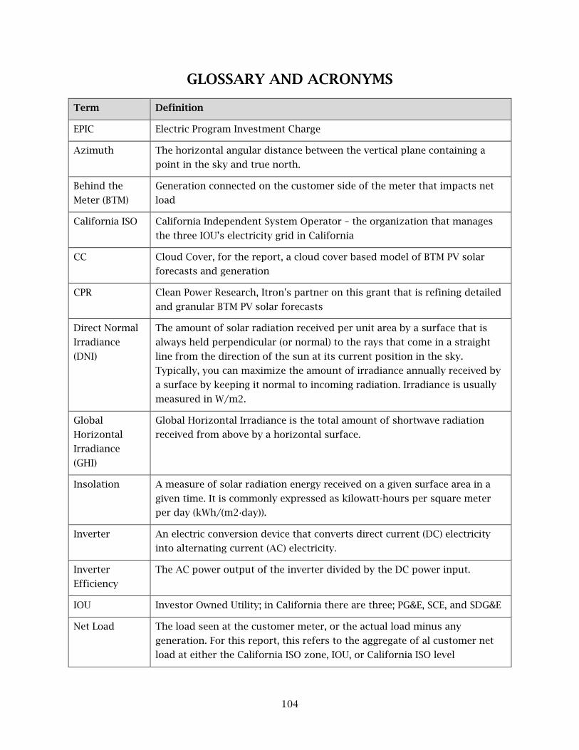
104

GLOSSARY AND ACRONYMS

Term Definition

EPIC Electric Program Investment Charge

Azimuth The horizontal angular distance between the vertical plane containing a

point in the sky and true north.

Behind the

Meter (BTM)

Generation connected on the customer side of the meter that impacts net

load

California ISO California Independent System Operator – the organization that manages

the three IOU’s electricity grid in California

CC Cloud Cover, for the report, a cloud cover based model of BTM PV solar

forecasts and generation

CPR Clean Power Research, Itron's partner on this grant that is refining detailed

and granular BTM PV solar forecasts

Direct Normal

Irradiance

(DNI)

The amount of solar radiation received per unit area by a surface that is

always held perpendicular (or normal) to the rays that come in a straight

line from the direction of the sun at its current position in the sky.

Typically, you can maximize the amount of irradiance annually received by

a surface by keeping it normal to incoming radiation. Irradiance is usually

measured in W/m2.

Global

Horizontal

Irradiance

(GHI)

Global Horizontal Irradiance is the total amount of shortwave radiation

received from above by a horizontal surface.

Insolation A measure of solar radiation energy received on a given surface area in a

given time. It is commonly expressed as kilowatt-hours per square meter

per day (kWh/(m2·day)).

Inverter An electric conversion device that converts direct current (DC) electricity

into alternating current (AC) electricity.

Inverter

Efficiency

The AC power output of the inverter divided by the DC power input.

IOU Investor Owned Utility; in California there are three; PG&E, SCE, and SDG&E

Net Load The load seen at the customer meter, or the actual load minus any

generation. For this report, this refers to the aggregate of al customer net

load at either the California ISO zone, IOU, or California ISO level

105

Term Definition

Orientation The azimuth and tilt of a PV system.

PG&E Pacific Gas and Electric; the IOU that provides natural gas and electricity to

much of Northern California

SCE Southern California Edison; the IOU that provides electricity to much of

Southern California outside of San Diego

SDG&E San Diego Gas and Electric; the IOU that provides natural gas and electricity

to San Diego and the surrounding area

Solar

Irradiance

Radiant energy emitted by the sun, particularly electromagnetic energy.

Solar Noon The moment when the sun appears highest in the sky (nearest zenith),

compared to its positions during the rest of the day. It occurs when the sun

is transiting the celestial meridian.

Solar PV Solar Photovoltaic; a technology that uses semiconductors to convert solar

irradiance into DC electrical power. This DC electrical power is usually

converted to AC electrical power uses inverter(s).

HASP Hour Ahead Scheduling Process (HASP) is a process for scheduling energy

and ancillary services based on the bids submitted.

LMP Locational Marginal Pricing (LMP) is a way for wholesale electric energy

prices to reflect the value of electric energy at different locations,

accounting for the patterns of load, generation, and the physical limits of

the transmission system.

DAM Day Ahead Market (DAM) is a financial market where market participants

purchase and sell electric energy at financially binding day-ahead prices for

the following day.

106

REFERENCES

Itron White Paper, Forecast Practitioner’s Handbook: Incorporating the Impact of Embedded

Solar Generation into a Short-Term Load Forecasting Model,” (101376WP-01) 2014.

Monforte, F. and McMenamin J.S., “Short-Term Energy Forecasting with Neural Networks,” with

The Energy Journal, Volume 19, Number 4, 1998.

MacDonald et al, “Demand Response Providing Ancillary Services a Comparison of Opportunities

and Challenges in the US Wholesale Markets,” Grid-Interop Forum 2012.

Improving Solar and Load Forecasts by Reducing Operational ...

Documents

Transcript of Improving Solar and Load Forecasts by Reducing Operational ...