“Improving inventory management in a highly volatile

market”

Hottenhuis, W.G. (Wouter)

Bachelor IEM-student

BACHELOR THESIS

INDUSTRIAL ENGINEERING AND MANAGEMENT

I

Final Bachelor Thesis

Improving inventory management in a highly volatile market

2nd of September 2020

Author

Wouter Hottenhuis

Bachelor Industrial Engineering & Management

University of Twente.

Educational institution

University of Twente

Drienerlolaan 5

7522NB Enschede

The Netherlands

Supervisor University of Twente

Dr. Ir. E. A. Lalla-Ruiz

Faculty BMS, IEBIS

Second examiner University of Twente

Dr. I. Seyran Topan

Faculty BMS, IEBIS

Hosting company

TenCate Geosynthetics Netherlands B.V.

Europalaan 206

7559 SC Hengelo

The Netherlands

Supervisor TenCate Geosynthetics

Mr. H. Hagedoorn

Production Manager

II

THE VERSION OF THIS THESIS DOES NOT CONTAIN CONFIDENTIAL INFORMATION.

NUMBERS ARE MULTIPLIED BY A RANDOM NON-INTEGER VALUE AND SPECIFIC

PRODUCT INFORMATION IS LEFT OUT.

III

MANAGEMENT SUMMARY TenCate Geosynthetics is an internationally operating company, which is world’s leading

provider of geosynthetics and industrial fabrics. The company serves the global market with

facilities all over the world, of which one production facility in Hengelo (OV), The

Netherlands. After moving to a new facility, TenCate wants to focus on optimizing the

internal processes.

The problem that TenCate is facing was twofold: on the one hand did the company experience

too much inventory that was building up, and on the other hand did they experience too many

backorders and lost sales. These problems were, by using a problem cluster and going back in

the causal chain, reduced to an inventory management problem. After conducting interviews

with the problem owner and stakeholders, the following research question was formulated:

“How can TenCate make a proper forecast and have an adequate inventory management in a

highly volatile market?”

The research started by making an analysis of the current situation with respect to inventory

management. A flow-diagram was made of the internal process and underlying characteristics

were found. Demand of the products that were investigated is intermittent, irregular, random

and often even sporadic. No demand distribution can be found. Currently, safety stocks are

not calculated but minimum and maximum inventory levels are set based on the experience

and intuition of the planner. Next to that, the company currently does not monitor the

backorders and occurrences of lost sales.

After the current situation was clear, the literature was consulted. Basic concepts on inventory

management were retrieved and used to make a concept matrix to see the differences and

similarities between different safety stock models. In the literature also different kind of

indicators were found that could be used to measure the contribution of a new proposed safety

stock model. The total average inventory value was eventually chosen to be the main KPI

here for.

One important part of inventory management is making a good forecast. For the products of

TenCate this could not be done by using a probability function. Therefore, five different time-

series forecasting methods were compared. With a quantitative analyse the best forecasting

method for the products of TenCate was found to be the improved Croston method by the

researchers Teunter, Syntetos and Babai (2011). Next to that the most appropriate safety stock

model was chosen for TenCate. This was done in a qualitative way, by combining the analysis

of the current situation and the knowledge gather from the literature. The (R, s, S)-policy was

most favourable, which is a periodic reviewing model with a pre-set reorder point.

After that the final step in the research was made, a simulation was made by using the historic

data as input for the new proposed forecasting method and safety stock model. This

simulation showed that the new proposed inventory policy would higher the inventory value

by XX%. There are several explanations why the outcome of the model shows a raise in total

inventory. In short, the two main reasons are:

▪ Safety stock levels and reorder points are set for some products that would be more

applicable for a make-to-order policy instead of a make-to-stock policy.

IV

▪ The aimed service level of 90 % in the calculations is too high for the business in

which TenCate operates.

The core problem of not having calculated safety stock levels was solved. In this way, also the

starting problems were tackled. Therefore, the new proposed method does also have some

advantages. The company experienced too many backorders and meanwhile they had a lot of

inventories. Out of the calculations came that some products need higher safety stocks, and

others should have a reduction of safety stocks. This is probably respectively for the products

which had too many backorders and for the products that had on average too many

inventories. Besides that, with these higher inventories, more occurrences of lost sales could

be turned into actual sales, which will increase the inventory turnover.

To conclude the research, some recommendations and options for further research were made

based on the experience during the internship and the results of the research. The following

recommendations and options for further research are formulated and explained in the thesis:

▪ Include the capacity of the production hall in the research.

▪ Make a classification for all products at TenCate, use the ABC analysis.

▪ Make a clear distinction between MTO and MTS products.

▪ Find out whether emergency manufacturing orders are rewarding.

▪ Optimize communication between the sales-team and the planner.

▪ Monitor backorders and lost sales.

▪ Make a dashboard per business process for extra insights in the company’s

performance.

V

PREFACE Before you lie the thesis “Improving inventory management in a highly volatile market”. This

thesis is written in a final assignment for the finishing of my Bachelor Industrial Engineering

& Management at the University of Twente. The research that I did was conducted at TenCate

Geosynthetics in Hengelo (OV) in the Netherlands. Together with a supervisor at the

company and a supervisor of the University I was able to finalize my bachelors by writing this

thesis.

During the research I learned to use theories in practice. Applying these relatively simple

models to very complex situation that are completely different than examples out of study

books was quite challenging and exciting to me. Fortunately, this was something to be learned

during this period. In addition, my scientific way of thinking and the structuring of problem

solving is something that is now brought to a higher level.

I enjoyed the period as an intern at TenCate due to the open environment and friendly

colleagues. Especially I would like to express my sincere gratitude to company supervisor

Herald, for helping me where he could and trying to be of service to me.

In addition, I would like to thank my supervisor at the University of Twente: Dr. Ir. E.A.

Lalla-Ruiz for helping me writing this thesis. I am grateful for his critical way of thinking, his

punctuality, and new ideas that he gave me. Next to that, I am just so grateful to my second

examiner Dr. I. Seyran Topan for her expertise in the field of this research what she kindly

shared with me.

Last but not least, I would like to thank my family and friends for supporting me in any other

way during the past period.

I hope you enjoy reading this bachelor thesis,

Wouter Hottenhuis

Enschede, 2nd of September 2020

TABLE OF CONTENTS

MANAGEMENT SUMMARY ................................................................................................ II

PREFACE ................................................................................................................................. V

TERMS AND DEFINITIONS .............................................................................................. VIII

1 INTRODUCTION .............................................................................................................. 1

1.1 Company background .................................................................................................. 1

1.2 Research motivation .................................................................................................... 1

1.3 Problem context ........................................................................................................... 1

Action and core problem ................................................................................................. 2

Norm and reality .............................................................................................................. 3

1.4 Research questions ...................................................................................................... 3

1.5 Research design ........................................................................................................... 5

Thesis structure ................................................................................................................ 5

Limitation and scope ....................................................................................................... 6

Methodology ................................................................................................................... 6

Deliverables ..................................................................................................................... 7

Validity and reliability ..................................................................................................... 8

2 CURRENT SITUATION .................................................................................................... 9

2.1 Products and inventory management ........................................................................... 9

2.2 Business process and inventory management ........................................................... 10

Business process diagram .............................................................................................. 10

Characteristics of the company ..................................................................................... 11

2.3 Conclusion ................................................................................................................. 11

3 THEORETICAL FRAMEWORK .................................................................................... 12

3.1 Literature research ..................................................................................................... 12

Which concepts in the literature are relevant for safety stock models? ........................ 12

What safety stock models do exist in the literature and where do they differ on? ........ 13

3.2 Key performance indicators ....................................................................................... 16

Key performance indicators in the literature ................................................................. 16

KPI selection ................................................................................................................. 17

Current inventory value ................................................................................................. 17

3.3 Conclusion ................................................................................................................. 18

VII

4 FORECASTING AND SAFETY STOCKS ..................................................................... 19

4.1 Forecasting ................................................................................................................. 19

Cleaning data from outliers ........................................................................................... 19

Product choice ............................................................................................................... 20

Forecasting methods ...................................................................................................... 21

Selection of the most suitable forecasting method ........................................................ 25

Conclusion ..................................................................................................................... 30

4.2 Safety stocks .............................................................................................................. 31

Selecting a safety stock model ...................................................................................... 31

Determining the variables for the safety stock model ................................................... 33

4.3 Conclusion ................................................................................................................. 36

5 IMPLEMENTATION AND CONTRIBUTION .............................................................. 37

5.1 Linking the forecast to the safety stock model .......................................................... 37

5.2 Improvement on current situation .............................................................................. 38

5.3 Conclusion ................................................................................................................. 40

6 CONCLUSIONS & RECOMMENDATIONS ................................................................. 41

6.1 Conclusions ............................................................................................................... 41

6.2 Further research ......................................................................................................... 42

6.3 Recommendations ..................................................................................................... 43

7 BIBLIOGRAPHY ............................................................................................................. 46

Appendix A .............................................................................................................................. 49

Systematic literature research (subquestion 1) ..................................................................... 49

Systematic literature research (subquestion 2) ..................................................................... 52

Appendix B .............................................................................................................................. 55

Appendix C .............................................................................................................................. 56

Appendix D .............................................................................................................................. 57

VIII

TERMS AND DEFINITIONS

KPI: Key Performance Indicator. A quantitative value that expresses the performance of a

business, method or objectives.

ERP-system: Enterprise Resource Planning system. A software package that companies

generally use for all kind of processes within the company. Within the software these

processes are integrated to manage the processes adequately. Examples of these processes are

the planning, inventory, sales and financial processes.

MTO: Make-to-order. A production strategy that is order based. Every time an order arrives,

the production of the product(s) within that order starts. Generally used for products which are

highly customizable and/or very expensive.

MTS: Make to stock. A production strategy that is based on the level of inventory. The goal is

to match the inventory with the anticipated demand. Generally used for products that can be

made constantly and in large orders.

MPSM: Managerial Problem-Solving Method. A methodological checklist of steps to be

taken to come to solutions for knowledge and action problems.

Safety stock: inventory that is kept extra to reduce the risk of stockout.

Reorder point: the quantity of inventory which initiates a new (manufacturing) order.

Lot size: the quantity of an item ordered or manufactured in one single production run.

Backorders: an order that is already placed by the customer but could not be fulfilled directly

from stock because it is temporarily out of stock. The next time the item is on stock again, it

will be delivered to the customer.

Lost sales: potential sales that did not occur because the products could not be delivered on

time and the customer chooses to not buy the product.

Service level: a desired probability of meeting demand on time.

IFR: Item fill rate. A service level measure that calculates the percentage of all products that

are delivered on time.

OFR: Order fill rate. A service level measure that calculates the percentage of all orders that

are delivered on time. If only one product out of a large order cannot be delivered on time, the

whole order counts as a backorder which is delivered too late.

1 INTRODUCTION

In the introduction the company is first introduced. After that research motivation is

described and lastly the research question will be introduced together with subquestions that

will be used as guideline for this thesis.

1.1 Company background

The company where this thesis is made is TenCate. The company is divided in several business

groups, of which one, TenCate Geosynthetics, finding its roots in The Netherlands. TenCate

Geosynthetics is a company which has emerged from Nicolon BV, a Dutch company that made

strong and advanced industrial textiles. The company was innovative, it was taking a great deal

of progress with respect to the manufacturing of these textiles, which became stronger, rot

resistant, and more sustainable. After the flood disaster of 1953 in The Netherlands, the

company grows even faster because it is involved in a lot of flood prevention projects. To meet

production demand, the company opens a new facility in the United States of America. Quickly

after that, TenCate Geosynthetics was born.

Currently, TenCate Geosynthetics is an internationally operating company, which is world’s

leading provider of geosynthetics and industrial fabrics. The company serves the global market

with facilities all over the world, of which one production facility in Hengelo (OV).

1.2 Research motivation

The current problem TenCate Geosynthetics is facing, has emerged after moving to a new

facility in Hengelo in 2018. The reason for moving out of the old facility was because it was

getting too small. After setting up the machines in the new facility TenCate produces just as it

did for the past years. Currently in the new facility with everything set up, TenCate has time to

focus on improving and optimising their internal processes.

In the first few meetings with TenCate the main context of the problem was about not knowing

exactly how the facility was performing in Sales & Operations and what could be improved in

the Sales & Operations planning. After conducting interviews with the problem owners, the

management and the planner, the problem was narrowed down to an inventory management

problem.

1.3 Problem context

The current situation at TenCate is not as it is desired. Currently, the general feeling is that

“there are too many backorders and there are also too high stock levels”. This is thus seen as a

problem. On the other hand, they are keeping safety stocks following the best practice method.

During the last twenty years safety stock levels have not changed. The too high stock levels and

2

the backorders concern different products. The high stock levels cause a low inventory turnover

ratio, which can generally be described as not good. The inventory turnover ratio is calculated

with:

𝐼𝑛𝑣𝑒𝑛𝑡𝑜𝑟𝑦 𝑇𝑢𝑟𝑛𝑜𝑣𝑒𝑟 𝑅𝑎𝑡𝑖𝑜 = 𝐶𝑜𝑠𝑡 𝑜𝑓 𝐺𝑜𝑜𝑑𝑠 𝑆𝑜𝑙𝑑 ÷ 𝐴𝑣𝑒𝑟𝑎𝑔𝑒 𝐼𝑛𝑣𝑒𝑛𝑡𝑜𝑟𝑦

To lower the average inventory, and thus higher the inventory turnover ratio, one could look at

the safety stock levels. By doing so, it is also possible to solve the backorder problem.

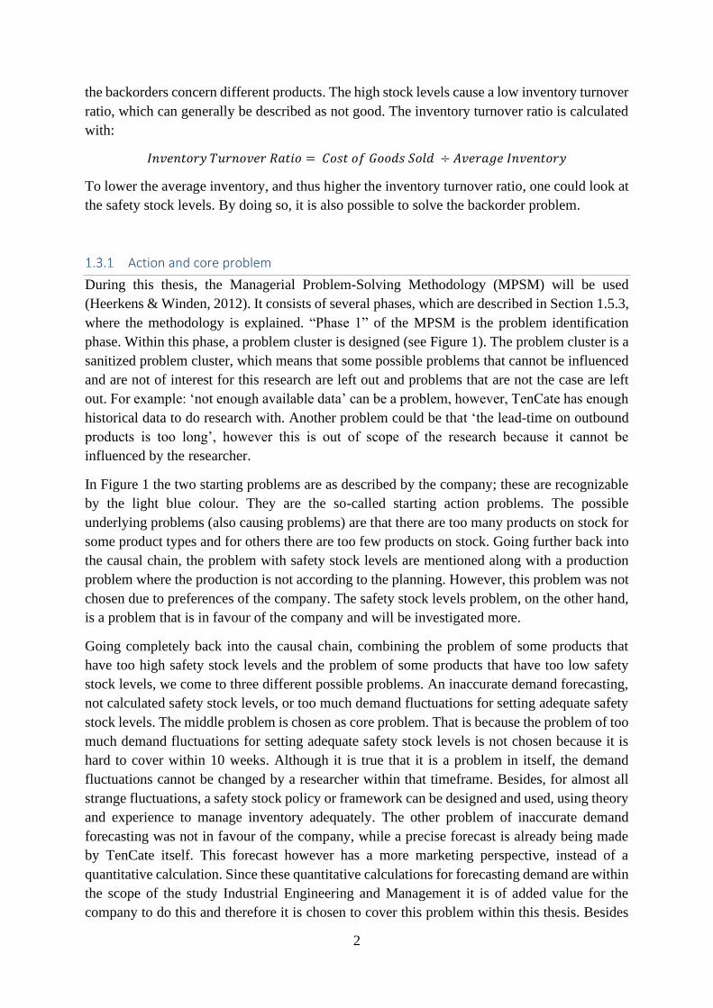
Action and core problem

During this thesis, the Managerial Problem-Solving Methodology (MPSM) will be used

(Heerkens & Winden, 2012). It consists of several phases, which are described in Section 1.5.3,

where the methodology is explained. “Phase 1” of the MPSM is the problem identification

phase. Within this phase, a problem cluster is designed (see Figure 1). The problem cluster is a

sanitized problem cluster, which means that some possible problems that cannot be influenced

and are not of interest for this research are left out and problems that are not the case are left

out. For example: ‘not enough available data’ can be a problem, however, TenCate has enough

historical data to do research with. Another problem could be that ‘the lead-time on outbound

products is too long’, however this is out of scope of the research because it cannot be

influenced by the researcher.

In Figure 1 the two starting problems are as described by the company; these are recognizable

by the light blue colour. They are the so-called starting action problems. The possible

underlying problems (also causing problems) are that there are too many products on stock for

some product types and for others there are too few products on stock. Going further back into

the causal chain, the problem with safety stock levels are mentioned along with a production

problem where the production is not according to the planning. However, this problem was not

chosen due to preferences of the company. The safety stock levels problem, on the other hand,

is a problem that is in favour of the company and will be investigated more.

Going completely back into the causal chain, combining the problem of some products that

have too high safety stock levels and the problem of some products that have too low safety

stock levels, we come to three different possible problems. An inaccurate demand forecasting,

not calculated safety stock levels, or too much demand fluctuations for setting adequate safety

stock levels. The middle problem is chosen as core problem. That is because the problem of too

much demand fluctuations for setting adequate safety stock levels is not chosen because it is

hard to cover within 10 weeks. Although it is true that it is a problem in itself, the demand

fluctuations cannot be changed by a researcher within that timeframe. Besides, for almost all

strange fluctuations, a safety stock policy or framework can be designed and used, using theory

and experience to manage inventory adequately. The other problem of inaccurate demand

forecasting was not in favour of the company, while a precise forecast is already being made

by TenCate itself. This forecast however has a more marketing perspective, instead of a

quantitative calculation. Since these quantitative calculations for forecasting demand are within

the scope of the study Industrial Engineering and Management it is of added value for the

company to do this and therefore it is chosen to cover this problem within this thesis. Besides

3

that, the forecasts can also be useful in assessing the contribution of the research by performing

a simulation. Therefore, see the figure below.

To summarize, after identifying the action problems, a problem cluster is built where the core

problem was found by going back into the causal chain. The core problem for this research is:

“Safety stock levels are not calculated”.

Norm and reality

According to Heerkens & Winden, it is important to assess whether a problem is solved within

a research. In their methodology: ‘MPSM’, they use the discrepancy between the norm and the

reality. It is necessary that the norm and reality are comparable. In the case of TenCate, the

norm is for all products safety stock levels are calculated. However, in reality the case is that

the safety stock levels are not calculated. The current safety stock levels are historical based

estimations of the sales team and some have not changed over twenty years.

The core problem describes a discrepancy between norm a reality. This problem does not need

an indicator to measure whether at the end the research the problem is tackled. That is because

it is self-evident when safety stock levels are calculated in the case of TenCate.

1.4 Research questions

Based on the interviews that were conducted and the problem cluster that is made, the main

research question is formulated. The main research question is:

“How can TenCate make a proper forecast and have an adequate inventory management in a

highly volatile market?”

Figure 1. Problem cluster for TenCate

4

In order to answer this question, sub-research questions were formulated. The answer to each

research question contributes to solving the core problem and answering the research question.

For the purpose of a good structure in the research, these questions are subcategorized in several

topics. Every research question will be explained shortly and will be accompanied with a

deliverable at the final version of the thesis.

Current situation

1) What does the current situation look like at TenCate with respect to inventory

management?

a. What does the current inventory policy look like and how does TenCate set

safety stock levels?

b. What does demand look like for the products at TenCate?

c. What effects does the inventory policy have on TenCate?

For the purpose of structuring question 1, subquestions a), b), and c) are added. With the

subquestions, the current situation for TenCate can be described in terms of inventory

management. The goal of this question is to get familiar with the business of TenCate and see

how they do their work normally. Info will be gathered by using semi-structured interviews and

walk-ins. This info can be useful in later stages in the research to compare the current situation

with the desired situation. By answering this question, an analysis of the current situation will

be delivered.

Literature research

2) Which concepts in the literature are relevant for safety stock models?

3) What safety stock models do exist in the literature and where do they differ on?

These questions can be answered by investigating the literature, specifically by doing a

systematic literatur review. Within the literature a lot can be found on inventory management

or safety stock models. The answer of subquestion 2 is used to answer subquestion 3. The goal

of these questions is to get insight in, and have a clear understanding of the existing models.

Doing so, the advantages and disadvantages can also be simply derived from the overview. By

anwering this question, a clear overview of different safety stock models is delivered.

4) Which key performance indicator can be used to analyse the contribution of this

research for TenCate?

Also this question is answered by addressing literature, however, this question is not answered

by a systematic literature research. Here, the literature and the knowledge of what the current

situation looks like (question 1) are combined. The answer to this question contributes to the

final thesis because the whole research can then be evaluated. For example by looking at the

total cost savings, number of backorders, or the inventory turnover. By answering this question,

one KPI will be chosen.

5

Methodology

5) Which forecasting method can best be used for the products of TenCate?

With a quantitative analysis a comparison is made between several forecasting methods that

could be applicable for the products at TenCate. By answering this question, one forecasting

method has been chosen which is used later in research question 8.

6) Which safety stock model can best be used for the products of TenCate?

After considering the research on the literature, a safety stock model is chosen based on the

characteristics of the business and products of TenCate. By answering this question, one safety

stock model is chosen.

7) What safety stock levels and parameters are best for the products of TenCate?

Along with the previous question, this question is also part of the core research. This question

will be answered with the outcome of Question 6. All data that is useful is used to come up with

the best safety stock levels for TenCate. By answering this question safety stock levels are

calculated and clarified.

Implementation and contribution

8) How do the calculated safety stock levels and forecasting method work out for TenCate?

This question is to evaluate the calculated safety stock levels. By linking the forecasts to the

safety stock model, it is possible to simulate the inventory management over the historic data.

The contribution can be measured by using the KPI that is found in question 4. By answering

this question, a simulation of the inventory management is made and the contribution of this

research to the company is measured and explained.

1.5 Research design

Thesis structure

The structure of this thesis is given by the following chapters:

▪ In Chapter 2 the research question 1 will be answered. Here the current situation is

closely examined.

▪ In Chapter 3 a systematic literature review is performed to find out what can be

learned from the theory about safety stock models, that is research question 2 and 3.

Besides, KPI’s are selected, which is research question 4. This KPI is used in the

evaluation, where the current situation is compared to the proposed situation.

▪ After that in Chapter 4, research question 6 is answered with the info of the

abovementioned chapters. After selecting the right safety stock model, question 7 can

6

be answered, where the right parameters will be calculated. Also, research question 5

is answered and the right forecasting model is chosen.

▪ Lastly research question 8 is answered in Chapter 8. Here the contribution of the

research is measured by using the information of research question 4.

For an overview of the structure within the thesis, see Figure 2.

Limitation and scope

Together with the company a scope was created for the research. This scope also takes some

limitations into account.

Time: the bachelor assignment takes up approximately 10 weeks at the company. This is a short

time frame; therefore, it is not possible to perform in depth research for every part. That means

that some simplifications need to be done during this thesis. That is explicitly stated at the

moment when this is done.

Business-units-scope: due to the time boundary mentioned above, not all business units of

TenCate can be covered. That is why, in cooperation with the company, it is decided the focus

will be on two business units, Business Unit 2 and Business Unit 3. These business units consist

of products that are responsible for a large amount of the output, which makes it interesting to

look at.

Methodology

The Managerial Problem-Solving Method (MPSM) (Heerkens & Winden, 2012) will be the

methodology that serves as the main guideline for problem solving. It is a problem-solving

method which consists of seven phases. The seven phases go from problem identification to the

analysis, to the decision and eventually an evaluation. The first phase ‘Problem identification’

is covered in the previous chapter.

In the two phases after that, ‘problem analysis’ and ‘solution generation’, we do research in

several research methods. Both quantitative and qualitative research methods are used.

Figure 2. Structure of subquestions within this thesis

7

Quantitative research methods are used in this thesis in the form of historical data. This data

will be merely demand, sales, and production data. This data is already made available for the

execution of this bachelor assignment

Qualitative research methods are used primarily when interviewing employees or management

members. The interview types that will be used are the unstructured and the semi-structured

interview. The unstructured interviews are the general conversations about the topic. These

conversations will mostly be held with the planner of TenCate. For the semi-structured

interviews, questions will be made prior to the interview, and during the interview questions

can be added and adjusted. This is a flexible way of interviewing and used for the elite

interviewing approach, for gathering information from well-informed or influential people in

the organization (Cooper & Schindler, 2014). Also, the forecast report of EMEA will be a

combination of qualitative and quantitative data.

To accomplish the research, one should structure its research. There are four types of research

mentioned by Cooper & Schindler that help us guide the research. This research will follow

both an explanatory and predictive scope. A previous systematic literature research (Hottenhuis,

2019) already went deeper into the different aspects of these types of studies. The systematic

literature research in that research was specific for the problem context of this thesis. The

predictive study is rooted in theory, which is also the case in this thesis. Future demands are

predicted, and corresponding safety stock levels will be calculated. However, this prediction

will be based on an explanatory hypothesis. So first an explanatory study is conducted: “The

explanatory study goes beyond description and attempts to explain the reasons for the

phenomenon that the descriptive study only observed” (Cooper & Schindler, 2014). This thesis

also goes beyond just describing phenomena and investigates what model is best for the

TenCate’s processes. Based on the model, the safety stock levels are calculated.

Besides the types of studies used, this work will also use another perspective. That is a technical

perspective; purely based on data, safety stock levels will be calculated. Also, a theoretical

research method is used by conducting a systematic literature research.

Finally, the solution implementation and evaluation will be addressed by using the methodology

of the MPSM. The implementation of the safety stock levels is out of the scope of this project,

however, a simulation will be performed to evaluate the results. Within this analysis historical

demand is used to evaluate the contribution of this research on the KPI chosen within the thesis.

Deliverables

During the thesis the research questions are answered. These answers and the way of working

are presented to the company by the following deliverables:

▪ An analysis of the current situation. This can give insights in the internal processes of

the company out of a theoretical point of view.

▪ A proposed forecasting method is presented. This is a method that should also give

proper forecasts when demand in intermittent or volatile.

8

▪ A proposed safety stock model is presented based on the characteristics of the

company and the literature.

Validity and reliability

The data that will be used in this project is data subtracted from an internal ERP-system, a

software program that only uses the raw data of the ERP-system, and insights from

conversations/interviews with employees of TenCate.

The validity of data is the concept that refers to how well a measure actually measures what is

intended to measure. The validity of the research is guarantee. That is done by means of

discussing all raw data intensively with more than one employee to make sure all numbers have

the same unit of measure and thus can be compared and used for research.

The reliability of the data will also be assessed and tried to be as reliable as possible. Because

it comes out of an ERP, sometimes data can be strangely ordered or formulated. When

retrieving data, the data will be assessed on whether there are no strange order lines in there.

This will also be discussed with the employees. On the other hand, also when interviewing

employees, the reliability of their statements will be tested by asking the same questions to

different people. In this way, all the biased and distorted statements will be remarked.

Besides the validity and reliability of the data, also the outcome has to be valid and reliable.

This will be assured by using valid and reliable data. Also, all outcomes and findings will be

presented unambiguously, by clearly formulating the results in words, tables and graphs. On

top of that, after the research, the report will be closed with a discussion, including a thorough

reflection and stating the limitations of the research to deliver an honest and reliable report.

9

2 CURRENT SITUATION

The research questions that will be addressed in this chapter is: “What does the current

situation look like at TenCate with respect to inventory management?”. The goal of this

question is to get familiar with the business of TenCate. Insights are gathered with respect to

inventory management.

2.1 Products and inventory management

TenCate currently produces around more than thousand different finished products. All these

products are divided in around 100 different product types. The product types differ on types

of material used, width of the product and the way its woven. Then every product type can be

processed and customized to how the customer it desires. This results in subassemblies,

products with extra treatments, or a different finishing. These customized products are the

thousands of different finished products.

TenCate uses a combination of a Make To Order (MTO) and a Make To Stock (MTS) process.

That means that sometimes production orders are linked to sales orders, and sometimes

production orders are to fill-up inventory, then they are linked to sales forecast. The reason why

the process is a combination of MTO and MTS is because of large demand fluctuations within

the business in which TenCate operates. These fluctuations are in the amount of orders as well

as in the size of the orders. That is why it is hard to estimate safety stock levels for the different

product types. Also, some orders are highly customized products for the customer, for obvious

reasons, these are also MTO products. The products that are considered appropriate for an MTS

process are chosen based on common sense and the general experience of the planner and the

sales team.

Currently, the sales team of TenCate came up with minimum and maximum safety stock levels

for the most important products that are MTS products. They came up with these numbers in

the same way as the categorization of MTO and MTS products: by their common sense and

general experience. Some of these minimum and maximum levels are updated, others are

already twenty years old. The planner looks every week at the current inventory levels, together

with the production planning, the incoming orders and the prognosis of upcoming demand, to

adjust the planning in such a way that orders can be shipped as soon as possible while safety

stock levels of other products are also between the minimum and maximum level.

This is exactly the trade-off to be made by the decision maker: the customer order response

time versus the safety stock level. Raising the safety stock levels will result in a more adequate

supply of finished goods to the customer when an order arrives, a quick delivery. However,

raising the safety stock level will also result in more inventory, which leads to more inventory

holding costs and handling costs. Besides, all this inventory has value and all money invested

in safety stock is not directly value-adding to the company. On the other hand, with low safety

stock levels, customer order response time goes down.

10

2.2 Business process and inventory management

Business process diagram

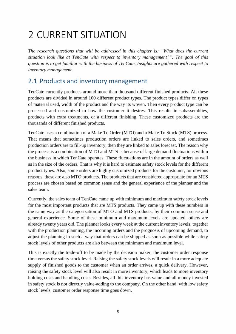
To give insight in the business process of TenCate, including different inventory types, a

business process diagram is made (see Figure 3. Business process diagram of TenCate). Two

starting events are identified. First, when a customer order arrives and secondly when the

inventory drops below a specific level. Both of them are discussed below.

When a customer order arrives, the inventory is checked to see whether the products in the

order are available. If this is the case, the order can be delivered on short term; two options are

possible. The order consists of a product or more products that are in the intermediate inventory.

These products can then be shipped immediately and are thus the MTS products. It is also

possible, in the other case, that the product needs some finishing. Most of the time, this is done,

by combining several woven materials to an end product. After that, the product can be

delivered. Going back, it is also possible that the order is not in the inventory. That is most of

the time the case. The products that are generally in these orders are the so called “MTO

products”. Often, in cooperation with the planner and the customer, a delivery date is set, and

the planner will keep tracks that the order can be shipped on time.

The other starting point is when inventory drops below a certain pre-set level. At that moment,

when production capacity allows, a new production order is placed, to fill up to the desired

inventory level. Important is that this event is not directly triggered when inventory drops below

the minimum. That is because TenCate makes use of a periodic reviewing system. So once a

week it is checked whether the inventory has dropped below the pre-set level.

Both intermediate inventory and outbound inventory are in the same warehouse. The focus of

this thesis is on the intermediate inventory, with in particular the woven materials. These items

are important because they are sometimes shipped directly to the customer and also important

for the assembly for some orders. By improving safety stock levels in this inventory, the most

impact can be made.

Figure 3. Business process diagram of TenCate

11

Characteristics of the company

A complete overview of the business process can be described through the main characteristics

of the company.

1. Lot sizes:

Lot sizes refers to the quantity of an item that is manufactured in a single production run.

In the previous section, the initiating event for a production order was stated. Production

orders are generally running for a long time at TenCate. For one batch, this can take up to

14 weeks on 1 creel. During production, depending on the specific product that is woven, a

couple of times per day a semi-finished product can be placed in the inventory. Hence, lot

sizes are big, but inventory is filled up constantly when a product is being made.

2. Lost sales:

Lost sales are the selling opportunities that are lost because an item was out of stock.

Currently, Ten Cate has no insight in lost sales because they do not monitor this. That has

a lot to do with inventory management, since most of the lost sales come from not being

able to deliver when the customer wants. When increasing the safety stock levels, one is

able to deliver on more short term, and might then be able to close a deal which is probably

a large one, since it could not be fulfilled with the lower safety stock level.

3. Service level / backordering:

The service level is a fraction of the orders or products that are delivered on time. That is in

the business of TenCate hard to calculate because not all delivery dates are strict. Sometimes

it is possible that TenCate is running behind on the production schedule. When clearly

communicating the expected new delivery date with the customer, it is possible that they

agree on a new, later delivery date. However, it is not possible to trace back how often this

happens. That means that backorders cannot be retrieved from the data, backorders are also

not monitored. Next to that, another possibility is that the customer contacts TenCate with

the notification that they want to receive their products later. In that case, TenCate cannot

send the products as planned again, and has to make a trade-off to prioritize other customers.

4. Demand

In general, the demand is perceived as highly volatile and intermittent. In semi-structured

interviews for example, it was told that sometimes a demand occurrence could be three

times more than the total demand of the previous year. This demand and possible patterns

will be discussed and investigated later on in this thesis.

2.3 Conclusion

TenCate is clearly in a business with many characteristics that are not found in the typical study

book. Hence, assumptions need to be made to try to select the best safety stocks. These

assumptions will be described explicitly when they need to be made. Now the characteristics

of the TenCate are clear. The next chapter will cover a theoretical study to answer more research

questions.

12

3 THEORETICAL FRAMEWORK

In Chapter 0 the explanation is found which theoretical framework this research consists of.

Also, subquestion 2 and 3 will be answered by doing a systematic literature review: “Which

concepts in the literature are relevant for safety stock models?” and “What safety stock

models do exist in the literature and where do they differ on?”. Lastly, subquestion 4 will be

answered by addressing the literature to find out how to measure the contribution of this

thesis by selecting a key performance indicator.

This research is about safety stock models. However, within the literature a lot of different

terms are used for the same concept. Terms as ‘inventory system’ (Bijulal et al. 2011, Porras &

Dekker 2008, Olhager & Persson 2006), ‘inventory model’ (Wang 2011), ‘inventory method’

(Sani & Kingsman 1997), inventory policy (Aardal et al. 1989), safety stock planning (Beutel

& Minner 2012) or safety stock model (Van Donselaar & Broekmeulen 2013) are widely

described and all come down to the same underlying content. To ensure that this thesis is

coherent and consistent, this thesis will use the term safety stock model. This includes all

guidelines in setting safety stock levels. Another definition to have clear is that of safety stocks:

safety stocks are additional quantities of a product held in inventory to reduce the risk of that

product from being out of stock.

3.1 Literature research

In order to answer one of the subquestions, a systematic literature research is conducted.

Two questions, as described in Chapter 1, are answered. First it is necessary to know how to

address safety stock models in order to compare them:

1) Which concepts in the literature are relevant for safety stock models?

2) What safety stock models do exist in literature and where do they differ on?

This division is made because, when evaluating safety stock models, it is convenient to compare

them on some concepts. For the search strings used for this research, the management of the

findings, and the conceptual matrix, please see Appendix A. Below the subquestions will be

shortly introduced and the main findings are described before answering the question.

Which concepts in the literature are relevant for safety stock models?

In the literature all kinds of concepts and variables are mentioned to take into account when

calculating safety stock levels or choosing a safety stock model. A parallel theme of the research

in analysing control policies is based on system perfomance measures. Examples of these

system performance measures are service levels and costs. Order fill rate (OFR) and item fill

rate (IFR) are the two main service level measures. These are measures that are often being

stressed (Kok 1985, Bijulal et al. 2011, Kang et al. 2017). The OFR takes the percentage of all

13

orders that are fulfilled on time as a service level. It does not take into account whether a order

is lacking all items within the order or only one item that could not be delviered. However, the

IFR takes the percentage of all items that are met on time. Another concept that is taken into

account, a little less often, is the number of backorders are considered when evaluating safety

stock levels (Braglia et al. 2014, Yadollahi et al. 2016). In order to achieve a certain service

level or number of backorders, safety stocks are kept in inventory to capture the fluctuations in

demand. These demand fluctuations are described in the majority of the literature. They typicily

assume a given theoretical demand distribution and estimate the required parameters from

historical data. Some works describe the arrival of orders as a Poisson proces (Kok 1985), others

assume a Normal distribution of the total ordered products (Bijulal et al. 2011, Sellitto 2018,

Klosterhalfen & Minner 2010), but sometimes work is published on non-parametric demand

(Beutel & Minner, 2012). Besides the service level performance measure, a lot of work

concerns the cost performance measure, where they strive for a minimum cost solution

(Tempelmeier 2013). Frequently the holding costs and ordering costs are taken into account.

Purchasing costs is not necessary to take into account when safety stocks are calculated for

manufacturers (Kang et al. 2017). Every piece of work is about its specific field of study. This

literature research focused on the coherence and differences between the different papers.

The most important concepts to take into account when assessing different safety stock models

are the total costs, the demand, and the service level. These are generic concepts, however, the

service level can be calculated in different ways. These concepts help to guide the comparison

of safety stock models and are used as a springboard to the next subquestion, where different

safety stock models are addressed.

What safety stock models do exist in the literature and where do they differ on?

The assessment of the different safety stock models is done by addressing the concepts that

were found as most important in the previous subquestion.

In the literature different safety stock models are often referred to as policies. Every research

uses its own abbreviations for the variables within such a policy. The general (r, Q)-policy and

(s, S)-policy are described very often because they are relatively simple (Winston 2004, Porras

& Dekker 2008, Sani & Kingsman 1997, Aardal et al. 1989). The ‘r’ is the reorder point in this

policy and the ‘Q’ the number of products to be reordered. In the (s, S) model the s stands for

reorder point and the ‘S’ for the maximum level of inventory to which it should be raised. Some

literature can also be found on (r, Q)-policies where the objective function is not made with a

stockout-cost component, but where it is replaced with a service-level constraint. (Aardal et al.

1989). Other work describe these basic policies but adjusted it a little bit, for example the (s-1,

S)-model (Moinzadeh et al. 1991) or the (R, S)-policy (Van Donselaar & Broekmeulen 2013,

Winston 2004), which are respectively a one-by-one ordering policy and a periodic review

policy. This is something where policies differ on, continuous or periodic reviewing. A periodic

review policy has the practical advantage over a continuous review policy that a periodic review

policy is easier to administer since you need to review your current inventory just a few

moments in time. Policies can also be combined, which is the case in a (R, s, S)-policy

(Grubbström & Wikner 1996, Van Donselaar & Broekmeulen 2013), where every ‘R’ units in

14

time it is checked whether the reorder point ‘s’ is reached to order up to ‘S’ products. Then

there are also inventory models with a lot of feedback loops which controls the whole system

(Bijulal et al. 2011). By using system dynamics, all relationships between the variables are

considered and taken into account when adjusting safety stock levels.

Besides the differences in continuous versus periodic reviewing, a reorder point versus an order

up to level, and all little nuances in the models, all these models come with their corresponding

relationship with the three concepts of the previous section. This can be found in the concept

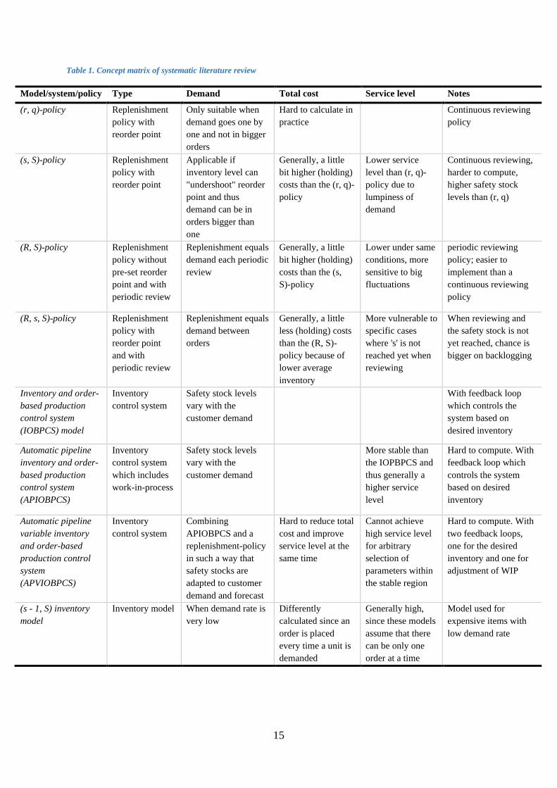
matrix, the table on the next page, Table 1.

Table 1 has several columns. Each row represents a safety stock model that was found in the

literature. At the column second column the type of policy is described to quickly distinguish

the different types of safety stock models. Then the three columns next to that are describing

extra info, based on the concepts that were found in the literature to be relevant. Further notes

are placed in the last column.

The justification of the literature review can be found in Appendix A. There is an overview of

the search strings used for this research and the management of the findings. Eventually the

concept matrix was made. This table that is made by conceptual thinking. Different safety stock

models are compared to identify underlying similarities and differences. The table is a concisely

written. Eventually, this will be used later on in the thesis. By understanding these differences

between the safety stock models will, together with the concept matrix, enable answering the

research questions later in the thesis.

15

Table 1. Concept matrix of systematic literature review

Model/system/policy Type Demand Total cost Service level Notes

(r, q)-policy Replenishment

policy with

reorder point

Only suitable when

demand goes one by

one and not in bigger

orders

Hard to calculate in

practice

Continuous reviewing

policy

(s, S)-policy Replenishment

policy with

reorder point

Applicable if

inventory level can

"undershoot" reorder

point and thus

demand can be in

orders bigger than

one

Generally, a little

bit higher (holding)

costs than the (r, q)-

policy

Lower service

level than (r, q)-

policy due to

lumpiness of

demand

Continuous reviewing,

harder to compute,

higher safety stock

levels than (r, q)

(R, S)-policy Replenishment

policy without

pre-set reorder

point and with

periodic review

Replenishment equals

demand each periodic

review

Generally, a little

bit higher (holding)

costs than the (s,

S)-policy

Lower under same

conditions, more

sensitive to big

fluctuations

periodic reviewing

policy; easier to

implement than a

continuous reviewing

policy

(R, s, S)-policy Replenishment

policy with

reorder point

and with

periodic review

Replenishment equals

demand between

orders

Generally, a little

less (holding) costs

than the (R, S)-

policy because of

lower average

inventory

More vulnerable to

specific cases

where 's' is not

reached yet when

reviewing

When reviewing and

the safety stock is not

yet reached, chance is

bigger on backlogging

Inventory and order-

based production

control system

(IOBPCS) model

Inventory

control system

Safety stock levels

vary with the

customer demand

With feedback loop

which controls the

system based on

desired inventory

Automatic pipeline

inventory and order-

based production

control system

(APIOBPCS)

Inventory

control system

which includes

work-in-process

Safety stock levels

vary with the

customer demand

More stable than

the IOPBPCS and

thus generally a

higher service

level

Hard to compute. With

feedback loop which

controls the system

based on desired

inventory

Automatic pipeline

variable inventory

and order-based

production control

system

(APVIOBPCS)

Inventory

control system

Combining

APIOBPCS and a

replenishment-policy

in such a way that

safety stocks are

adapted to customer

demand and forecast

Hard to reduce total

cost and improve

service level at the

same time

Cannot achieve

high service level

for arbitrary

selection of

parameters within

the stable region

Hard to compute. With

two feedback loops,

one for the desired

inventory and one for

adjustment of WIP

(s - 1, S) inventory

model

Inventory model When demand rate is

very low

Differently

calculated since an

order is placed

every time a unit is

demanded

Generally high,

since these models

assume that there

can be only one

order at a time

Model used for

expensive items with

low demand rate

16

3.2 Key performance indicators

The literature is studied to find out how the contribution of this research will be measured. In

combination with the knowledge collected in the previous chapters; the problem identification

and the characteristics of TenCate, KPIs are investigated. The situation that TenCate is currently

facing is that there is not yet a KPI where they review their inventory policy on. To analyse the

contribution of this research to the company, a comparison is made between TenCate’s

performance in the current situation with respect to inventory management, and the outcome of

this research. This comparison will be done quantitively. To do so, one can look at multiple

KPIs.

Key performance indicators in the literature

Regarding the goal of adept inventory management, the literature describes different goals or

KPIs. The KPIs that are mentioned in various works are found in the list below.

▪ Firstly, various works describe that the total costs savings is the most important for

companies which are trying to improve on inventory management (Kang et al, 2017 &

Tempelmeier, 2013). A side note that these researchers do place, is that it is hard to

come up with and to calculate a total cost function. That is because various types of

costs are hard to estimate, for example holding costs.

▪ Other researchers, such as Braglia et al. (2014) and Yadollahi et al. (2016) argue that

the number of backorders should be minimized. That is for attaining a good service

level, which is another KPI.

▪ The service level can be optimized by reducing the number of backorders. The customer

satisfaction and the company’s reputation are higher when lowering these backorders.

There are two kind of measures: SLM1, where the expected fraction of all demand that

is met on time is calculated, and SLM2, where the expected number of cycles per year

during which a shortage occurs is calculated (Winston, 2004). Both service level

measures are argued to be more important than the other. However, these service level

measures are not very applicable in the characteristic business of TenCate, where they

use a combination of producing MTO and MTS.

▪ Li (1992) argues that in a case of a choice between MTO and MTS policies, the speed

of delivery is where to compete on. He proposes two aspects, or indicators, that can lead

to a reduction of the customer waiting time. Firstly, the reduction of production lead

times, and secondly, increasing inventories to reduce customer waiting time.

▪ Also inventory turnover ratio (as described in Chapter 1) can be of use for measuring

the performance of inventory management. That tells the company for how long an item

is already in inventory. It is calculated by dividing the cost of goods sold by the average

inventory value.

17

KPI selection

After finding out what KPIs were often used for the reviewing of inventory management, the

right KPI will be selected for this thesis and for the company. This is done by looking at the

characteristics of the company and taking the company side perspective into account.

The total cost savings are hard to calculate, as stated in the previous section. The company

also do not have estimations for all kinds of costs that should be incorporated in that KPI.

Therefore, together with the company, it was decided that this KPI is not useful for this thesis.

Also, the number of backorders and the service level were found to be not appropriate for the

evaluation of the research. That is because currently these numbers are not monitored, so

there is no data to compare. The KPIs that were mentioned in the work of Li (1992), are also

not selected to be used. That is because the production lead times are out of the scope of this

thesis and not found to be a problem since they cannot be influenced. Next to that the

customer waiting time, as described at the company’s characteristics, is again an indicator

which cannot be retrieved from the data because it is not monitored.

Lastly the inventory turnover can be used. In Chapter 1 the formula was introduced. The

turnover ratio is calculated by two dividing the costs of goods sold by the average inventory

value. Since ‘the costs of goods sold’ cannot be influenced by the researcher, the focus will be

on the average inventory value. This was also approved by TenCate.

Current inventory value

To be able to compare the results of this research in comparison with the current situation, we

also need to know what inventory value is attained now. The data of the min-max inventory

levels for the products that are taken into consideration for this research were processed. The

desired inventory is the average between the min-max levels, since it is tried that the inventory

is always kept between these values.

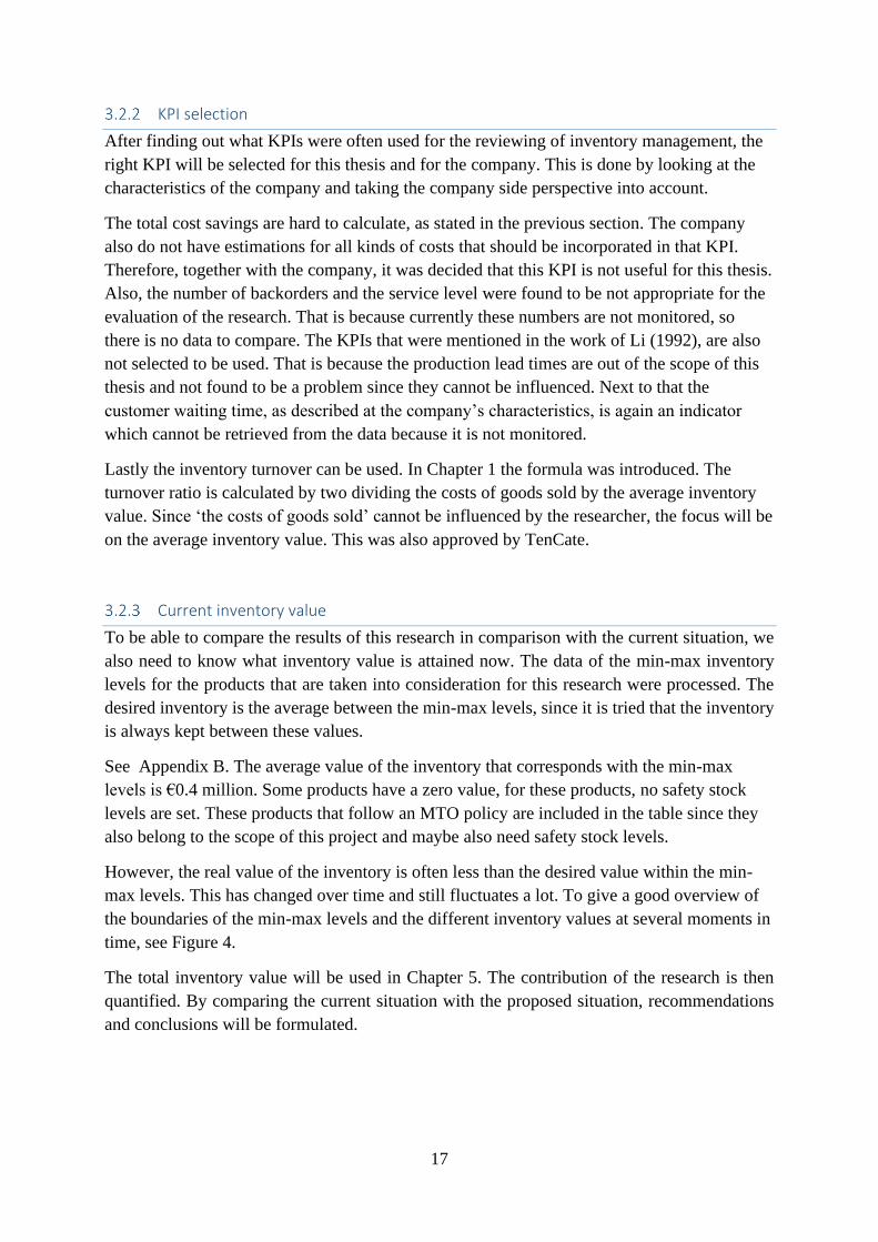
See Appendix B. The average value of the inventory that corresponds with the min-max

levels is €0.4 million. Some products have a zero value, for these products, no safety stock

levels are set. These products that follow an MTO policy are included in the table since they

also belong to the scope of this project and maybe also need safety stock levels.

However, the real value of the inventory is often less than the desired value within the min-

max levels. This has changed over time and still fluctuates a lot. To give a good overview of

the boundaries of the min-max levels and the different inventory values at several moments in

time, see Figure 4.

The total inventory value will be used in Chapter 5. The contribution of the research is then

quantified. By comparing the current situation with the proposed situation, recommendations

and conclusions will be formulated.

18

3.3 Conclusion

In this chapter the literature gave more insights in what safety stock models exist. Also,

different indicators were retrieved from the literature. Together with the company, one

indicator was chosen as main KPI. This will be used later in Chapter 5. The knowledge on

safety stock models will be used in the next chapter, Chapter 4.

Figure 4. min-max levels inventory value of TenCate

19

4 FORECASTING AND SAFETY STOCKS

Subquestion 5 will be covered in this chapter: “Which forecasting method can best be used

for the products of TenCate?” This chapter has added value to the project since the level of

the safety stocks will be set by using a forecasting method. At the end of this chapter one

forecasting method is chosen. Also, the current situation is investigated more closely in

combination with the knowledge on different safety stock models that was found in the

literature study. In this chapter, subquestion 6: “Which safety stock model can best be used

for the products of TenCate?” will also be answered. Eventually a safety stock model will be

chosen for the products of TenCate. After selecting a safety stock model, the safety stock

levels will be calculated.

4.1 Forecasting

A specific part of inventory management concerns forecasting. With forecasting one can make

a prediction of the future by looking and historical data. In this chapter different forecasting

methods will be investigated. At the end of this chapter, one forecasting method is chosen that

fits best for the products of TenCate. This will be done by using common metrics to measure

the accuracy of the forecast.

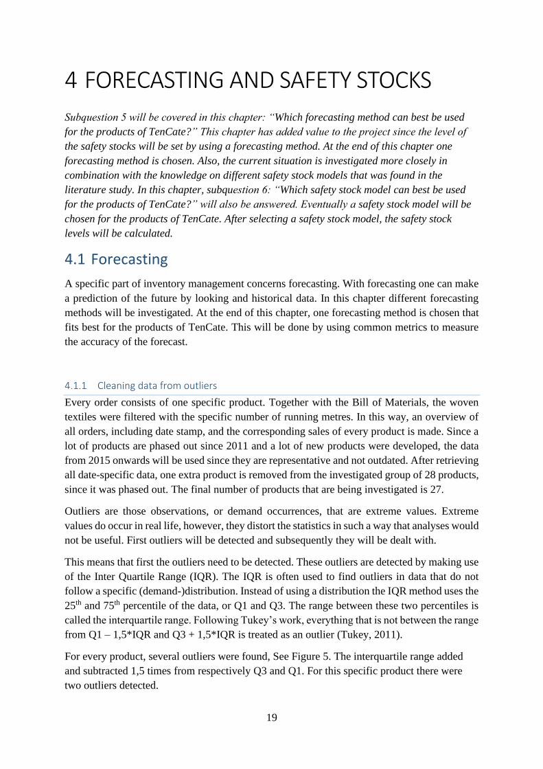
Cleaning data from outliers

Every order consists of one specific product. Together with the Bill of Materials, the woven

textiles were filtered with the specific number of running metres. In this way, an overview of

all orders, including date stamp, and the corresponding sales of every product is made. Since a

lot of products are phased out since 2011 and a lot of new products were developed, the data

from 2015 onwards will be used since they are representative and not outdated. After retrieving

all date-specific data, one extra product is removed from the investigated group of 28 products,

since it was phased out. The final number of products that are being investigated is 27.

Outliers are those observations, or demand occurrences, that are extreme values. Extreme

values do occur in real life, however, they distort the statistics in such a way that analyses would

not be useful. First outliers will be detected and subsequently they will be dealt with.

This means that first the outliers need to be detected. These outliers are detected by making use

of the Inter Quartile Range (IQR). The IQR is often used to find outliers in data that do not

follow a specific (demand-)distribution. Instead of using a distribution the IQR method uses the

25th and 75th percentile of the data, or Q1 and Q3. The range between these two percentiles is

called the interquartile range. Following Tukey’s work, everything that is not between the range

from Q1 – 1,5*IQR and Q3 + 1,5*IQR is treated as an outlier (Tukey, 2011).

For every product, several outliers were found, See Figure 5. The interquartile range added

and subtracted 1,5 times from respectively Q3 and Q1. For this specific product there were

two outliers detected.

20

The outliers were processed after the detection. The data is processed, by what is called:

winsorizing. Winsorizing is a way of handling with outliers. Instead of excluding the outliers

from the dataset they are replaced by the maximum that is allowed, in this case Q3 + 1,5*IQR.

These values are still of importance for the company and in this way, they are not neglected and

still part of the data set. In total, divided over the 27 products, 68 of the 1073 records were

winsorized.

Product choice

To choose an appropriate forecasting method in the next paragraph, all five methods are used

and visualised in a graph for all 27 products. The data that is used is the processed data with

winsorized outliers.

Since not each of the 27 products with all the graphs and numbers will be thoroughly explained

within this written part of the thesis, several selected products will be used to visualize the

calculations. For the other products the same calculations will be done. The selection of the

products that will be shown here is not done randomly. These products will be selected

carefully, because the selection of these products needs to be a reflection that represents the

whole product group. In order to do that, the products are divided into three categories. Since

one of the main characteristics of the demand pattern of TenCate’s products is the intermittency

of it, the most logical variable to base the categories on is the amount of intermittency.

The three categories were made. To express the amount of intermittency, the probability of a

demand occurrence is calculated. For example, when we use ‘one week’ as a time measure and

there is on average a demand occurrence every other week, the probability of a demand

occurrence will be 50%. Three categories were made: from 0% up until 33%, 34% up until

Dem

and

in lo

ngi

ng

met

ers

Demand outliers

Figure 5. Demand outliers - 1,5 * IQR

21

67% and 68% up until 100%. Out of each category one product was selected to be used as an

example to clarify the use of the chosen methods in this thesis. The best comparison is made if

the three products do not differ on any other variable, but the probability of a demand

occurrence. For that reason, the products that were eventually chosen also do have a comparable

overall demand over the same period of time. The total range of average demand in meters over

the time period is from 115 to almost 10.000 meters. The products that were chosen, have an

average demand between 500 meters and 1.000 meters.

See the following three products in the table below, these have been selected for the comparison

of the forecasting methods in this thesis. For the other items Appendix C gives an overview of

the data.

Table 2. Selected products with demand characteristics

Product Average demand (m) Probability of demand occurrence

PRODUCT A 198 90,2 %

PRODUCT B 112 58,8 %

PRODUCT C 123 29,4 %

Forecasting methods

4.1.3.1 Demand patterns

The data is now processed to make it more useful for analysis, calculations, and statistics.

Before beginning directly with calculating different forecasts, first the demand is investigated

more closely. That means that the data has now been first visualised. That is done to spot

potential trends, seasonality, or demand distributions. Unfortunately, these characteristics could

not be seen with the naked eye. That is why the data was also tested in Excel on for example

Poisson distributions or normal distributions, and in the program ‘CurveExpert’. With both

programs all outcomes of possible distributions and formulas were far off the mark.

Lon

gin

g m

eter

s

Example of demand behaviour

Figure 6. Example of the demand behaviour of a product at TenCate

22

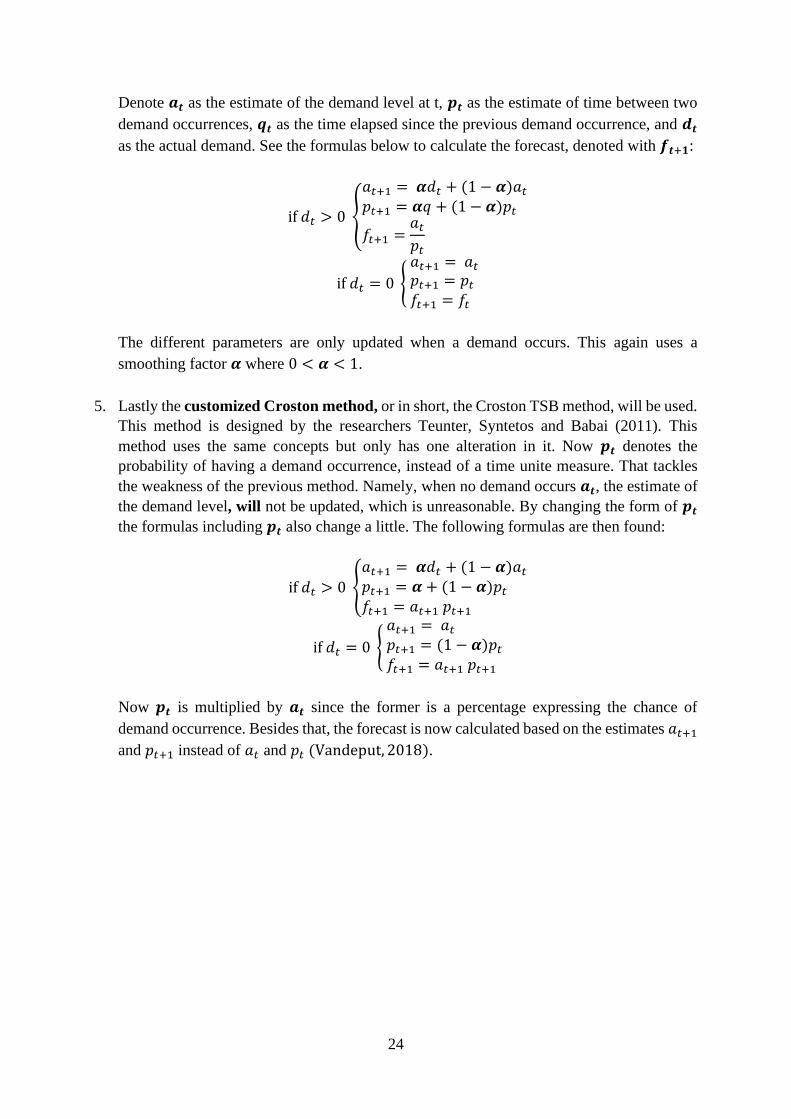
The demand, as can be seen in Figure 6. Example of the demand behaviour of a product at

TenCate, at TenCate is thus irregular, random and sometimes sporadic. Amongst others, for

that reason, no demand distribution could match with the products at TenCate.

4.1.3.2 Comparing forecasting methods

In total five different forecasting methods will be tested on their performance for the products

of TenCate. The methods differ on several things, for example the amount of historic time

events that are taken into account when forecasting the new period and the complexity of the

method. The forecasting methods that are eventually selected to be tested in this thesis are: the

naïve forecasting method, the moving average method, simple exponential smoothing, the

Croston method (Croston, 1972), and a Croston method that is later customized by other

researchers (Teunter, Syntetos, & Babai, 2011), that is called the Croston TSB method. These

are all time series forecasting methods and are chosen instead of using forecasting methods that

are based on demand distributions. That is because it could not be managed to find a proper

demand distribution to the products of TenCate.

Below the five methods that are mentioned above will be explained:

1. The naïve forecasting method is a relative straightforward method and is the least complex

one that is being described and compared in this thesis. The forecast for the next period is

the observation of the current period. Put in a formula it will be:

𝑓𝑡+1 = 𝑑𝑡 ,

where 𝑓𝑡+1 is the forecast for the period after time t and where 𝑑𝑡 denotes the actual

demand at time t. The advantage of the naïve forecasting method is that it is not hard to

implement. Besides that, research has shown that is some cases, especially in the financial

market, the naïve forecast performs better that other forecasting methods used by

(financial) analysts (Brooks & Gray, 2001). Therefore, it is interesting to see whether this

forecasting method is applicable for a business in which TenCate operates.

2. The moving average method is a forecasting method where the average of the last N

observations equals the forecast of the next period. After that period, the average will then

be calculated again with the last N observations, which means that the boundaries of the N

observations move one time unit, that is why it is called the moving average method. The

simple moving average method is used, which formula is as follows:

𝑓𝑡+1 =1

𝑁 ∑ 𝑑𝑡−𝑖

𝑁−1

𝑖=0

The same variables as in the previous forecasting method are used, namely 𝑓 and 𝑑. There

is still one variable that needs to be determined: the number of observations that are used to

calculate the forecast, the number N. Cooper et al. (2014) suggest that a value of N that will

minimize the mean absolute error should be choosen. This will make sure that the best

23

possible moving average method will be used in the comparison with the other methods.

The N is also called the order of the moving average method.

To do so, a forecasting error indicator will be used. This will be discussed in the next

paragraph.

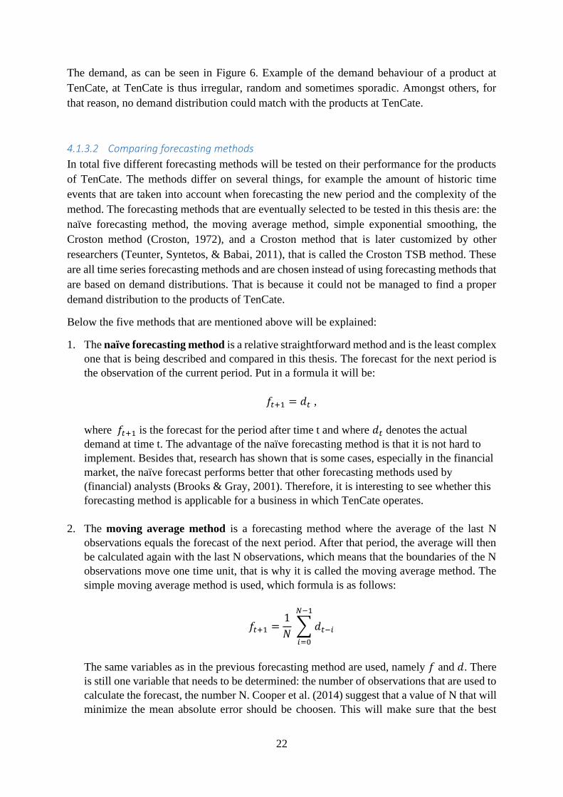
3. Simple exponential smoothing is the most ordinary form of time series forecasting. The

forecast is made each period based on all historic data. The model retrieves its name from

the fact that every data point is taken into account but decreases exponentially every time

unit. The formula as described by Cooper et al. (2014) to calculate the forecast is:

𝑓𝑡+1 = 𝜶𝑑𝑡 + (1 − 𝜶)𝑓𝑡

In which alpha is a ratio that satisfies 0 < 𝜶 ≤ 1. This ratio determines how much weight

is put on the last observation, and subsequently, on the previous forecast. The 𝑑𝑡 denotes

again the actual demand at time t. By changing alpha, one will change the level of

smoothing. That is why alpha is also called the smoothing factor. This alpha is determined

in the next paragraph.

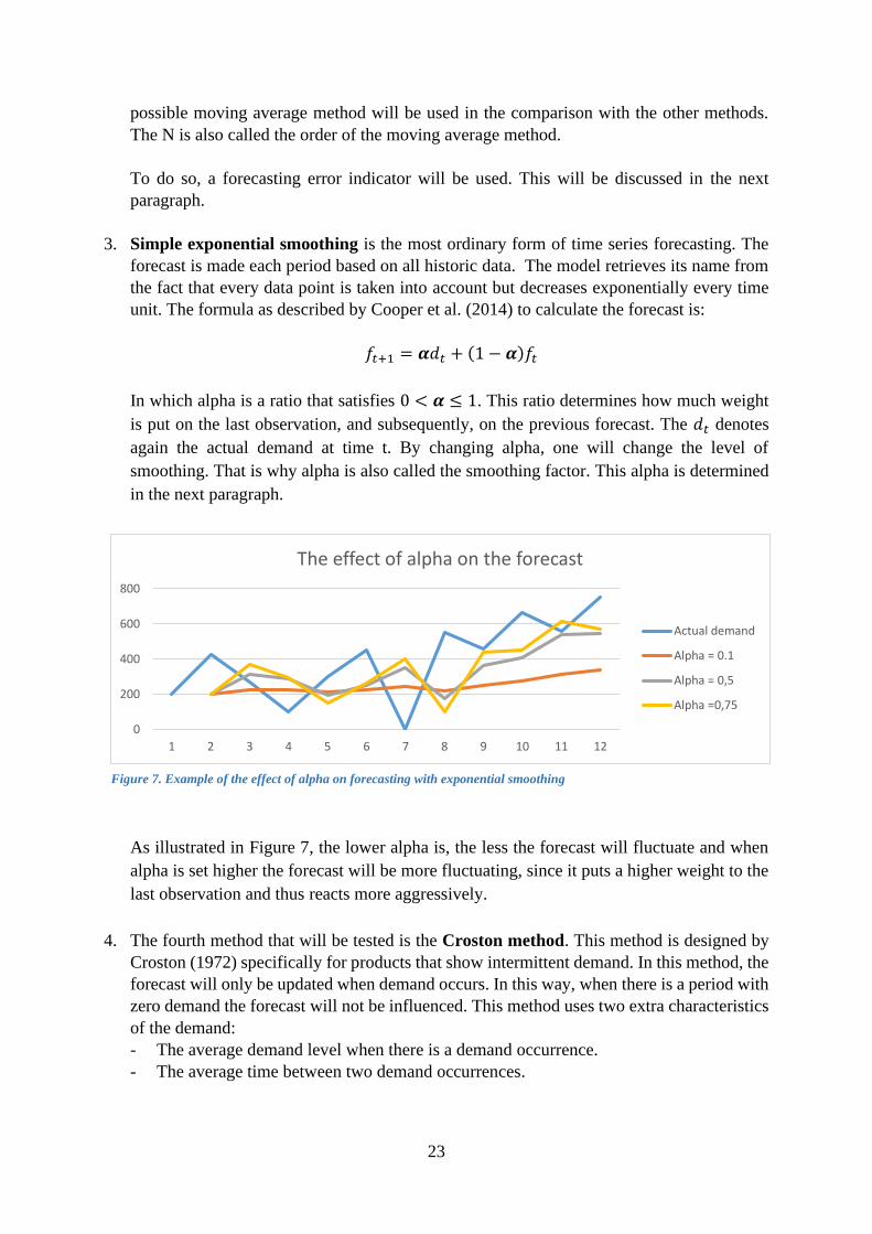
As illustrated in Figure 7, the lower alpha is, the less the forecast will fluctuate and when

alpha is set higher the forecast will be more fluctuating, since it puts a higher weight to the

last observation and thus reacts more aggressively.

4. The fourth method that will be tested is the Croston method. This method is designed by

Croston (1972) specifically for products that show intermittent demand. In this method, the

forecast will only be updated when demand occurs. In this way, when there is a period with

zero demand the forecast will not be influenced. This method uses two extra characteristics

of the demand:

- The average demand level when there is a demand occurrence.

- The average time between two demand occurrences.

0

200

400

600

800

1 2 3 4 5 6 7 8 9 10 11 12

The effect of alpha on the forecast

Actual demand

Alpha = 0.1

Alpha = 0,5

Alpha =0,75

Figure 7. Example of the effect of alpha on forecasting with exponential smoothing

24

Denote 𝒂𝒕 as the estimate of the demand level at t, 𝒑𝒕 as the estimate of time between two

demand occurrences, 𝒒𝒕 as the time elapsed since the previous demand occurrence, and 𝒅𝒕

as the actual demand. See the formulas below to calculate the forecast, denoted with 𝒇𝒕+𝟏:

if 𝑑𝑡 > 0 {

𝑎𝑡+1 = 𝜶𝑑𝑡 + (1 − 𝜶)𝑎𝑡

𝑝𝑡+1 = 𝜶𝑞 + (1 − 𝜶)𝑝𝑡

𝑓𝑡+1 =𝑎𝑡

𝑝𝑡

if 𝑑𝑡 = 0 {

𝑎𝑡+1 = 𝑎𝑡

𝑝𝑡+1 = 𝑝𝑡

𝑓𝑡+1 = 𝑓𝑡

The different parameters are only updated when a demand occurs. This again uses a

smoothing factor 𝜶 where 0 < 𝜶 < 1.

5. Lastly the customized Croston method, or in short, the Croston TSB method, will be used.

This method is designed by the researchers Teunter, Syntetos and Babai (2011). This

method uses the same concepts but only has one alteration in it. Now 𝒑𝒕 denotes the

probability of having a demand occurrence, instead of a time unite measure. That tackles

the weakness of the previous method. Namely, when no demand occurs 𝒂𝒕, the estimate of

the demand level, will not be updated, which is unreasonable. By changing the form of 𝒑𝒕

the formulas including 𝒑𝒕 also change a little. The following formulas are then found:

if 𝑑𝑡 > 0 {

𝑎𝑡+1 = 𝜶𝑑𝑡 + (1 − 𝜶)𝑎𝑡

𝑝𝑡+1 = 𝜶 + (1 − 𝜶)𝑝𝑡

𝑓𝑡+1 = 𝑎𝑡+1 𝑝𝑡+1

if 𝑑𝑡 = 0 {

𝑎𝑡+1 = 𝑎𝑡

𝑝𝑡+1 = (1 − 𝜶)𝑝𝑡

𝑓𝑡+1 = 𝑎𝑡+1 𝑝𝑡+1

Now 𝒑𝒕 is multiplied by 𝒂𝒕 since the former is a percentage expressing the chance of

demand occurrence. Besides that, the forecast is now calculated based on the estimates 𝑎𝑡+1

and 𝑝𝑡+1 instead of 𝑎𝑡 and 𝑝𝑡 (Vandeput, 2018).

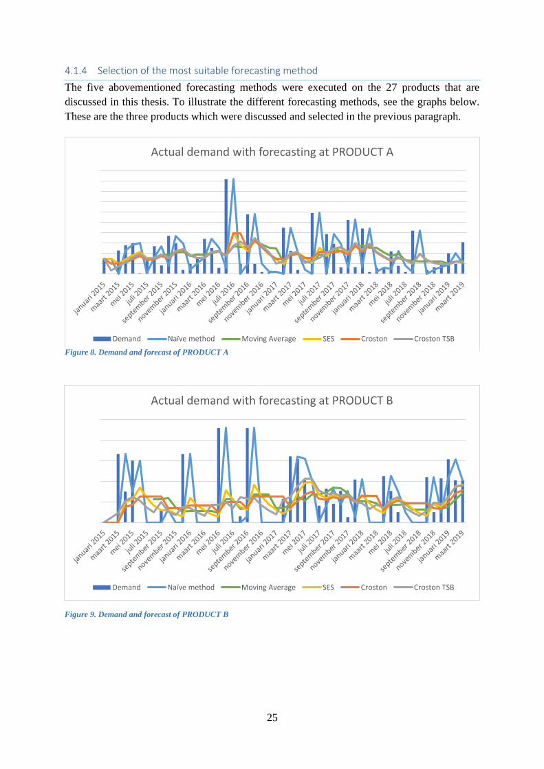
25

Selection of the most suitable forecasting method

The five abovementioned forecasting methods were executed on the 27 products that are

discussed in this thesis. To illustrate the different forecasting methods, see the graphs below.

These are the three products which were discussed and selected in the previous paragraph.

Actual demand with forecasting at PRODUCT A

Demand Naïve method Moving Average SES Croston Croston TSB

Actual demand with forecasting at PRODUCT B

Demand Naïve method Moving Average SES Croston Croston TSB

Figure 8. Demand and forecast of PRODUCT A

Figure 9. Demand and forecast of PRODUCT B

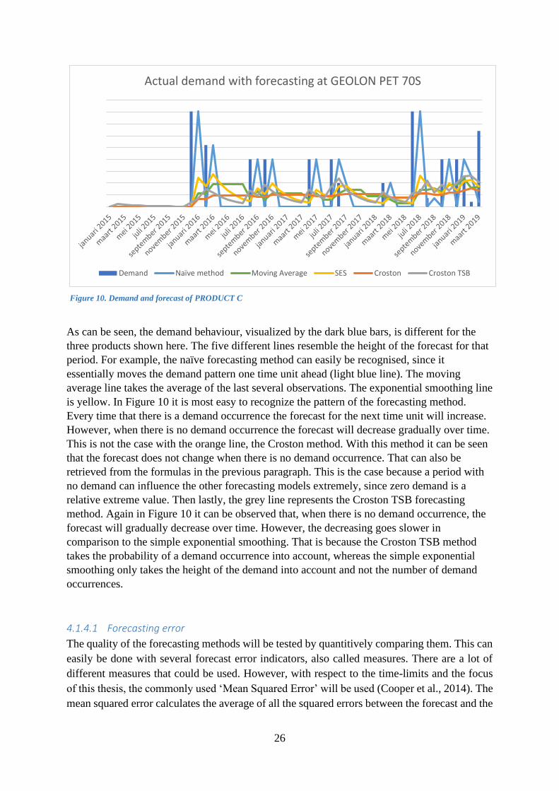
26

As can be seen, the demand behaviour, visualized by the dark blue bars, is different for the

three products shown here. The five different lines resemble the height of the forecast for that

period. For example, the naïve forecasting method can easily be recognised, since it

essentially moves the demand pattern one time unit ahead (light blue line). The moving

average line takes the average of the last several observations. The exponential smoothing line

is yellow. In Figure 10 it is most easy to recognize the pattern of the forecasting method.

Every time that there is a demand occurrence the forecast for the next time unit will increase.

However, when there is no demand occurrence the forecast will decrease gradually over time.

This is not the case with the orange line, the Croston method. With this method it can be seen

that the forecast does not change when there is no demand occurrence. That can also be

retrieved from the formulas in the previous paragraph. This is the case because a period with

no demand can influence the other forecasting models extremely, since zero demand is a

relative extreme value. Then lastly, the grey line represents the Croston TSB forecasting

method. Again in Figure 10 it can be observed that, when there is no demand occurrence, the

forecast will gradually decrease over time. However, the decreasing goes slower in

comparison to the simple exponential smoothing. That is because the Croston TSB method

takes the probability of a demand occurrence into account, whereas the simple exponential

smoothing only takes the height of the demand into account and not the number of demand

occurrences.

4.1.4.1 Forecasting error

The quality of the forecasting methods will be tested by quantitively comparing them. This can

easily be done with several forecast error indicators, also called measures. There are a lot of

different measures that could be used. However, with respect to the time-limits and the focus

of this thesis, the commonly used ‘Mean Squared Error’ will be used (Cooper et al., 2014). The

mean squared error calculates the average of all the squared errors between the forecast and the

Actual demand with forecasting at GEOLON PET 70S

Demand Naïve method Moving Average SES Croston Croston TSB

Figure 10. Demand and forecast of PRODUCT C

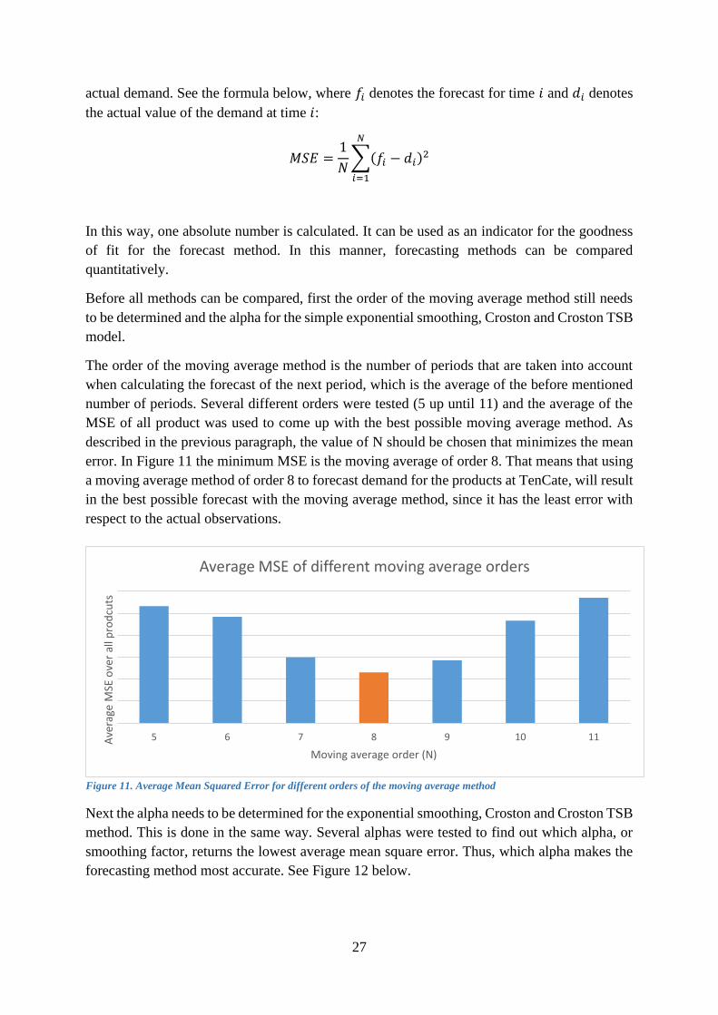
27

actual demand. See the formula below, where 𝑓𝑖 denotes the forecast for time 𝑖 and 𝑑𝑖 denotes

the actual value of the demand at time 𝑖:

𝑀𝑆𝐸 =1

𝑁∑(𝑓𝑖 − 𝑑𝑖)2

𝑁

𝑖=1

In this way, one absolute number is calculated. It can be used as an indicator for the goodness

of fit for the forecast method. In this manner, forecasting methods can be compared

quantitatively.

Before all methods can be compared, first the order of the moving average method still needs

to be determined and the alpha for the simple exponential smoothing, Croston and Croston TSB

model.

The order of the moving average method is the number of periods that are taken into account

when calculating the forecast of the next period, which is the average of the before mentioned

number of periods. Several different orders were tested (5 up until 11) and the average of the

MSE of all product was used to come up with the best possible moving average method. As

described in the previous paragraph, the value of N should be chosen that minimizes the mean

error. In Figure 11 the minimum MSE is the moving average of order 8. That means that using

a moving average method of order 8 to forecast demand for the products at TenCate, will result

in the best possible forecast with the moving average method, since it has the least error with

respect to the actual observations.

Next the alpha needs to be determined for the exponential smoothing, Croston and Croston TSB

method. This is done in the same way. Several alphas were tested to find out which alpha, or

smoothing factor, returns the lowest average mean square error. Thus, which alpha makes the

forecasting method most accurate. See Figure 12 below.

5 6 7 8 9 10 11Ave

rage

MSE

ove

r al

l pro

dcu

ts

Moving average order (N)

Average MSE of different moving average orders

Figure 11. Average Mean Squared Error for different orders of the moving average method

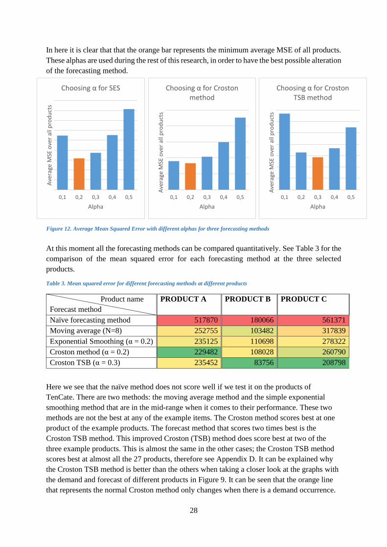
28

In here it is clear that that the orange bar represents the minimum average MSE of all products.

These alphas are used during the rest of this research, in order to have the best possible alteration

of the forecasting method.

At this moment all the forecasting methods can be compared quantitatively. See Table 3 for the

comparison of the mean squared error for each forecasting method at the three selected

products.

Table 3. Mean squared error for different forecasting methods at different products

Here we see that the naïve method does not score well if we test it on the products of

TenCate. There are two methods: the moving average method and the simple exponential

smoothing method that are in the mid-range when it comes to their performance. These two

methods are not the best at any of the example items. The Croston method scores best at one

product of the example products. The forecast method that scores two times best is the

Croston TSB method. This improved Croston (TSB) method does score best at two of the

three example products. This is almost the same in the other cases; the Croston TSB method

scores best at almost all the 27 products, therefore see Appendix D. It can be explained why

the Croston TSB method is better than the others when taking a closer look at the graphs with

the demand and forecast of different products in Figure 9. It can be seen that the orange line

that represents the normal Croston method only changes when there is a demand occurrence.

Product name

Forecast method

PRODUCT A PRODUCT B PRODUCT C

Naïve forecasting method 517870 180066 561371

Moving average (N=8) 252755 103482 317839

Exponential Smoothing (α = 0.2) 235125 110698 278322

Croston method (α = 0.2) 229482 108028 260790

Croston TSB (α = 0.3) 235452 83756 208798

0,1 0,2 0,3 0,4 0,5

Ave

rage

MSE

ove

r al

l pro

du

cts

Alpha

Choosing α for SES

0,1 0,2 0,3 0,4 0,5

Ave

rage

MSE

ove

r al

l pro

du

cts

Alpha

Choosing α for Croston method

0,1 0,2 0,3 0,4 0,5

Ave

rage

MSE

ove

r al

l pro

du

cts

Alpha

Choosing α for Croston TSB method

Figure 12. Average Mean Squared Error with different alphas for three forecasting methods

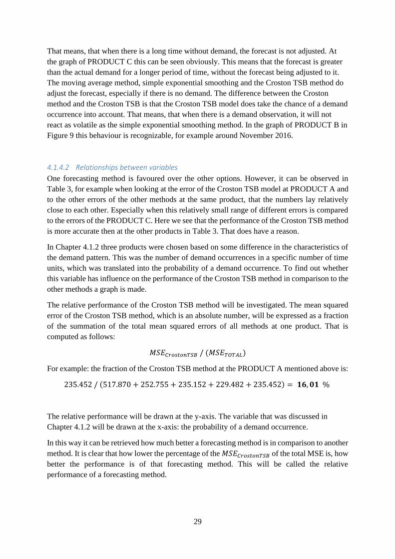
29

That means, that when there is a long time without demand, the forecast is not adjusted. At

the graph of PRODUCT C this can be seen obviously. This means that the forecast is greater

than the actual demand for a longer period of time, without the forecast being adjusted to it.

The moving average method, simple exponential smoothing and the Croston TSB method do

adjust the forecast, especially if there is no demand. The difference between the Croston

method and the Croston TSB is that the Croston TSB model does take the chance of a demand

occurrence into account. That means, that when there is a demand observation, it will not

react as volatile as the simple exponential smoothing method. In the graph of PRODUCT B in

Figure 9 this behaviour is recognizable, for example around November 2016.

4.1.4.2 Relationships between variables

One forecasting method is favoured over the other options. However, it can be observed in

Table 3, for example when looking at the error of the Croston TSB model at PRODUCT A and

to the other errors of the other methods at the same product, that the numbers lay relatively

close to each other. Especially when this relatively small range of different errors is compared

to the errors of the PRODUCT C. Here we see that the performance of the Croston TSB method

is more accurate then at the other products in Table 3. That does have a reason.

In Chapter 4.1.2 three products were chosen based on some difference in the characteristics of

the demand pattern. This was the number of demand occurrences in a specific number of time

units, which was translated into the probability of a demand occurrence. To find out whether

this variable has influence on the performance of the Croston TSB method in comparison to the

other methods a graph is made.

The relative performance of the Croston TSB method will be investigated. The mean squared

error of the Croston TSB method, which is an absolute number, will be expressed as a fraction

of the summation of the total mean squared errors of all methods at one product. That is

computed as follows:

𝑀𝑆𝐸𝐶𝑟𝑜𝑠𝑡𝑜𝑛𝑇𝑆𝐵 / (𝑀𝑆𝐸𝑇𝑂𝑇𝐴𝐿)

For example: the fraction of the Croston TSB method at the PRODUCT A mentioned above is:

235.452 / (517.870 + 252.755 + 235.152 + 229.482 + 235.452) = 𝟏𝟔, 𝟎𝟏 %

The relative performance will be drawn at the y-axis. The variable that was discussed in

Chapter 4.1.2 will be drawn at the x-axis: the probability of a demand occurrence.

In this way it can be retrieved how much better a forecasting method is in comparison to another

method. It is clear that how lower the percentage of the 𝑀𝑆𝐸𝐶𝑟𝑜𝑠𝑡𝑜𝑛𝑇𝑆𝐵 of the total MSE is, how

better the performance is of that forecasting method. This will be called the relative

performance of a forecasting method.

30

In Figure 13 all 27 products that are shown that are being investigated. In can be seen that there

is a relationship between the chance of a demand occurrence and the performance of the Croston

TSB. That means that the products which have a more intermittent demand will also score even

better compared to the other forecasting methods. This is an interesting relationship and can be

useful for the company to consider when forecasting with this method or for future use when

forecasting products with intermittent demand.

Conclusion

In this chapter a forecasting method is chosen that is most suitable for the products at TenCate.

By firstly processing the data and winsorizing outliers, the data was suitable to be used for

forecasting. Five different forecasts methods were investigated. It can be concluded that the

Croston TSB method is the most suitable for TenCate’s products. Remarkable is that it is found

that this method is even better compared to the other investigated methods when the demand of

the products is more intermittent.

R² = 0,5722

0,1

0,11

0,12

0,13

0,14

0,15

0,16

0,17

0,18

0,19

0,2

0 0,2 0,4 0,6 0,8 1 1,2

Rel

ativ

e p

erfo

rman

ce o

f C

rost

on

TSB

Chance of demand occurence

Performance of Croston TSB

Figure 13. The relative performance of the Croston TSB method with different demand occurrence probabilities

31

4.2 Safety stocks

In Chapter 3, the characteristics of the business and company were pointed out and explained.

After that, in Chapter 4 the literature was studied in order to have an overview of available

safety stock models, therefore also see Table 1 for the concept matrix. Now by combining these

two types of information, a safety stock model can be selected that is most appropriate for

TenCate.

A summary of the characteristics of the company is as follows:

- Currently, safety stock levels are set by the planner based on his experience and his

intuition. He came up with minimum and maximum safety stock levels.

- The running time for production is long, so lot sizes are large, however, when producing

the demand will be filled up constantly.

- There is no insight in lost sales. It is also not be possible to gather this from data.

- A reliable service level cannot be calculated in the business of TenCate.

- Demand is intermittent, irregular, random and often even sporadic. No demand

distribution can be found.

Selecting a safety stock model

By linking characteristics of both the safety stock model and the company to each other, a

safety stock model will be selected. The selection of a safety stock model will be done by

qualitatively comparing the models on some criteria. Three different criteria will be used.

These criteria were chosen based on the information that is already in the concept matrix in

Appendix A. The criteria, were the safety stock models will be reviewed at, are:

1. The overlap with the scope of this study.

Within the systematic literature review there was no distinction made between whether

a safety stock model is within the scope of the study Industrial Engineering and

Management or not. Only models that are within the scope of this study should be

chosen. That means, for example, that no extremely complex mathematical models

will be selected. That is because after choosing the model, the actual safety stock level

needs to be calculated with the knowledge that is gathered within the study of IEM.

2. The practical use.

Since TenCate works with one planner, who also has other responsibilities during a

week, they only make a planning once a week. In the safety stock models a distinction

can be made between the continuous reviewing models and the periodic reviewing

models. The periodic reviewing models score better when it comes to the practical use

for TenCate. Also, a continuous reviewing method is harder and more expensive to

implement in a company.

3. The fixed order sizes.

The last criterium that the models will be reviewed on is the presence or absence of a

fixed order size that comes with the model. In the concept matrix we see that some

32

models assume that ordering or manufacturing can be done one-by-one, some assume

that it is variable, and some assume that sizes of orders are fixed.

In the table below, every safety stock policy out of the concept matrix was given a plus (‘+’)

or a minus (‘–’) on every criterium, respectively for being suitable or not suitable.

Table 4. Overview of a qualitatively comparison between safety stock models for choosing the right model for TenCate

Model Scope Practical use Fixed order size

(r, q)-policy + – –

(s, S)- policy + – +

(R, S)- policy + + –

(R, s, S)- policy + + +

IOBPCS- policy – – –

APIOBPCS- policy – – –

APVIOBPCS- policy – – –

(s-1, S)- policy + + –

The safety stock models that turn out to be out of the scope of this study are the three models

described by Bijulal et al. (2011) in their paper, these are the IOBPCS-, APIOBPCS-, and

APVIOBPCS-policies. These models make use of system dynamics which is not covered in

the study area of this thesis (but in the study area of applied physics).

As described earlier, a division in safety stock models can be made by the reviewing period.

The two options that were identified were the continuous reviewing and the periodic reviewing.

A periodic reviewing method is more suitable from a practical point of view. In practice it is

hard for a company to continuously monitor the outflow of products out of the warehouse and

immediately produce new products when the reorder point is reached. It is easier and less

expensive to check the inventory on specific moments of time, for example in the beginning of

every week. That is why it is more suitable to choose a safety stock model with a periodic

reviewing time.

That means that the (R,S)-policy, the (R, s, S)-policy and (s-1, S) inventory model are the

models that are still suitable if the scope of the study and the reviewing period are taken into

account. The latter model has as advantage that it is used for expensive items with a low demand

rate. The principle is that the set-up or ordering costs outweigh the handling and holding costs

because the products are so expensive. However, this model is used at products where ordering

goes one by one. That is not applicable for TenCate where often orders are extremely large.

The final two options that are then left from the literature review are the (R, S)-policy and the

(R, s, S)-policy. The R stands for the review period and the capital S stands for the order-up-to

level. In the case of an (R, S)-policy, that means that every R units in time, the inventory level

is brought up to the level of S. As described in the introduction of this chapter, the lot sizes of

TenCate are very large. When, for example, during a period there has only been one small

demand occurrence it means that a creel must be set up and run for sometimes weeks to finish

the production. Subsequently, the order-up-to level is then largely overshot, resulting in higher

inventory levels than the targeted level S.

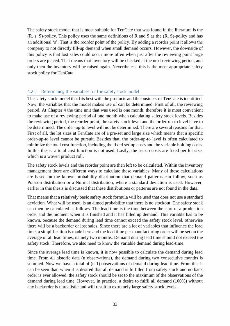
33

The safety stock model that is most suitable for TenCate that was found in the literature is the

(R, s, S)-policy. This policy uses the same definitions of R and S as the (R, S)-policy and has

an additional ‘s’. That is the reorder point of the policy. By adding a reorder point it allows the

company to not directly fill-up demand when small demand occurs. However, the downside of

this policy is that lost sales could occur more often when just after the reviewing point large

orders are placed. That means that inventory will be checked at the next reviewing period, and

only then the inventory will be raised again. Nevertheless, this is the most appropriate safety

stock policy for TenCate.

Determining the variables for the safety stock model

The safety stock model that fits best with the products and the business of TenCate is identified.

Now, the variables that the model makes use of can be determined. First of all, the reviewing

period. At Chapter 4 the time unit that was used is one month, therefore it is most convenient

to make use of a reviewing period of one month when calculating safety stock levels. Besides

the reviewing period, the reorder point, the safety stock level and the order-up-to level have to

be determined. The order-up-to level will not be determined. There are several reasons for that.

First of all, the lot sizes at TenCate are of a pre-set and large size which means that a specific

order-up-to level cannot be pursuit. Besides that, the order-up-to level is often calculated to

minimize the total cost function, including the fixed set-up costs and the variable holding costs.

In this thesis, a total cost function is not used. Lastly, the set-up costs are fixed per lot size,

which is a woven product roll.

The safety stock levels and the reorder point are then left to be calculated. Within the inventory

management there are different ways to calculate these variables. Many of these calculations

are based on the known probability distribution that demand patterns can follow, such as

Poisson distribution or a Normal distribution, where a standard deviation is used. However,

earlier in this thesis is discussed that these distributions or patterns are not found in the data.

That means that a relatively basic safety stock formula will be used that does not use a standard

deviation. What will be used, is an aimed probability that there is no stockout. The safety stock

can then be calculated as follows. The lead time is the time between the start of a production

order and the moment when it is finished and it has filled up demand. This variable has to be

known, because the demand during lead time cannot exceed the safety stock level, otherwise

there will be a backorder or lost sales. Since there are a lot of variables that influence the lead

time, a simplification is made here and the lead time per manufacturing order will be set on the

average of all lead times, namely two months. Demand during lead time should not exceed the

safety stock. Therefore, we also need to know the variable demand during lead-time.

Since the average lead time is known, it is now possible to calculate the demand during lead

time. From all historic data (n observations), the demand during two consecutive months is

summed. Now we have a total of (n-1) observations of demand during lead time. From that it

can be seen that, when it is desired that all demand is fulfilled from safety stock and no back

order is ever allowed, the safety stock should be set to the maximum of the observations of the

demand during lead time. However, in practice, a desire to fulfil all demand (100%) without

any backorder is unrealistic and will result in extremely large safety stock levels.

34

In order to visualize this statement, see Figure 14.

Here the y-axis depicts the safety stock value. The x-axis depicts the goal of the chance that in

a time unit (month) there is no stockout. That is the service level. So, in the previous example

where the maximum of the observations of demand during lead time was taken, the service

level would be 100%. In the figure it becomes clear that there is an exponential relationship

between the chance of no stockout and the level of safety stock that is kept. The difference in

safety stock that has to be kept extra when aiming at a service level of 97% instead of 95% is

in the figure almost 10 times as much money as the safety stock that has to be kept extra when

aiming at a service level of 87% instead of 85%. Besides that, it can be seen that a service level

of 100% that was sketched in the beforementioned example is unrealistic and unattainable.

An aim of a service level of 90% will be used. To aim for a service level of 90% the demand

during lead time will be used. From all the observations of the demand during lead time the 90th

percentile will be taken as the reorder point (ROP). The safety stock level (SS) can then be

calculated by the following formula:

𝑆𝑆 = 𝑅𝑂𝑃 − 𝐴𝑣𝑒𝑟𝑎𝑔𝑒 𝑆𝑎𝑙𝑒𝑠 ∗ 𝐴𝑣𝑒𝑟𝑎𝑔𝑒 𝐿𝑒𝑎𝑑 𝑇𝑖𝑚𝑒 ,

Where the average sales are per time unit, which is the monthly average sales. Filled in with

the terms described above, this becomes:

𝑆𝑆 = 90𝑡ℎ 𝑝𝑒𝑟𝑐𝑒𝑛𝑡𝑖𝑙𝑒 𝑜𝑓 𝑑𝑒𝑚𝑎𝑛𝑑 𝑑𝑢𝑟𝑖𝑛𝑔 𝑙𝑒𝑎𝑑 𝑡𝑖𝑚𝑒 − 𝑀𝑜𝑛𝑡ℎ𝑙𝑦 𝐴𝑣𝑒𝑟𝑎𝑔𝑒 𝑆𝑎𝑙𝑒𝑠 ∗ 2

To show how the 90th percentile is determined, see the table below, where we use PRODUCT

A as an example.

Table 5. Finding the Reorder Point

Figure 14. The relationship between the safety stock level and service level

35

Month Demand Demand during lead time

Ascending order

Position Percentile

Jan. 2015 157,592 157,6 21,1 1 0,02

Feb. 2015 0 240,1 42,1 2 0,04

Mar. 2015 240,121 533,9 42,2 3 0,06

Apr. 2015 293,797 607,6 42,5 4 0,08

May 2015 313,755 323,9 84,2 5 0,1

Jun. 2015 10,1726 178,7 105,3 6 0,12

Jul. 2015 168,48 452,4 105,3 7 0,14

Aug. 2015 283,952 371,6 111,4 8 0,16

Sep. 2015 87,630 477,3 115,0 9 0,18

Oct. 2015 389,635 702,1 126,4 10 0,2

Nov. 2015 312,509 354,6 147,4 11 0,22

Dec. 2015 42,12 147,4 157,6 12 0,24

Jan. 2016 105,3 273,8 161,6 13 0,26

Feb. 2016 168,48 526,5 178,7 14 0,28

… … … … … …

May 2018 231,66 315,90 622,3 41 0,82

Jun. 2018 84,24 105,30 622,3 42 0,84

Jul. 2018 21,06 463,32 623,6 43 0,86

Aug. 2018 442,26 442,34 702,1 44 0,88

Sep. 2018 0,0750 42,20 709,2 45 0,9

Oct. 2018 42,12 111,37 714,6 46 0,92

Nov. 2018 69,246 161,59 714,6 47 0,94

Dec. 2018 92,343 302,94 715,9 48 0,96

Jan. 2019 210,6 315,90 967,1 49 0,98

Feb. 2019 105,3 430,79 1030,3 50 1

Mar. 2019 325,48

cannot be

calculated

The table is divided in three parts. The left part is the processed data, it shows the demand per

month. After that, in the middle part of the table, the demand during lead time is calculated.

This is calculated by summing two consecutive periods, for example the first two months:

May 2015 + Jun 2015 = 313,755 + 10,1726 = 323,9 meters demand during lead time

After that, the demand during lead time is placed in ascending order in the right part of the

table. This ordered list of demand during lead time can then be used for calculating the 90th

percentile. Since there are 50 data point, the 90th percentile is found at the 45th position (50 *

0,9 = 45). This is 709,2 meters, and as earlier discussed, thus the reorder point that will satisfy

the aim of a service level of 90%. That is because in 90% of the occasions in the historic data,

the demand during lead time will not exceed 709,2 meters of this product.

The ROP is known, that means that the safety stock level can also be calculated now, using the

formula that wat presented above. In the case of PRODUCT A, the average monthly demand

equals 198. The lead time is 2 months. Substituting these numbers into the formula:

36

𝑆𝑆 = 90𝑡ℎ 𝑝𝑒𝑟𝑐𝑒𝑛𝑡𝑖𝑙𝑒 𝑜𝑓 𝑑𝑒𝑚𝑎𝑛𝑑 𝑑𝑢𝑟𝑖𝑛𝑔 𝑙𝑒𝑎𝑑 𝑡𝑖𝑚𝑒 − 𝑀𝑜𝑛𝑡ℎ𝑙𝑦 𝐴𝑣𝑒𝑟𝑎𝑔𝑒 𝑆𝑎𝑙𝑒𝑠 ∗ 2

𝑆𝑆 = 709,2 − 198 ∗ 2 = 313,2

That means that now all the variables are known for the safety stock model that best fits the

products for TenCate. In the case of this product, the reviewing period is one month, the safety

stock level is 312,3 meters and the reorder point is 709,2 meters. Every time the inventory drops

below the reorder point, one or several fixed lot sizes will be manufactured to fill up inventory

and bring it above the reorder point.

These calculations are also done for the other 26 products. All the calculated variables will be

used in the next chapter. The contribution of the research will there be addressed after

implementing the safety stock models with the forecasting method.

4.3 Conclusion

In Chapter 4 the data was processed. After cleaning the data from outliers, different forecasting

methods were tested. By making use of the mean square error, the smoothing factor was

optimized for every forecasting method and the order of the moving average method was found.

The Croston TSB method was the best forecasting method in general for the products at

TenCate. After that the safety stock model was chosen based on the characteristics of the

company that were found in Chapter 2. This model was the (R, s, S)-model. Lastly all

parameters were filled in for every product. In the next chapter the forecasting method will be

linked to the safety stock model to find out what the possible improvement is in terms of the

KPI that was chosen in Chapter 3.

37

5 IMPLEMENTATION AND CONTRIBUTION

Within this chapter, the eighth question will be answered: “How do the calculated safety stock

levels and forecasting method work out for TenCate?” This will be done by linking the forecasts

of Chapter 5 to the safety stock model of Chapter 6. With the known historic demand, the

inventory management will be simulated with the new proposed forecasting method and safety

stock policy. After that, it will be determined what the contribution of this research is to the

company. This will be done by making use of the KPI that was selected in Chapter 4.

5.1 Linking the forecast to the safety stock model

The safety stock model with the reorder point and the safety stock is known. The lot sizes are

different for each product and also known. That makes it able to simulate the inventory

management for each product with the chosen safety stock model, together with the forecasting

method. To explain on how this is done, the product PRODUCT A will again be used as an

example. See the table below, which is a part of a bigger table in Excel, which was used to

simulate the inventory management.

Table 6. Simulating inventory management

TABLE LEFT OUT FOR CONFIDENTIALLITY. BELOW A DESCRIBITON IS FOUND

The first row describes each month, the two rows after that are the demand, that was given in

the data of the company, and the forecast, that was calculated in Chapter 5. The five rows

below that are cells which all use formulas. To start with the fourth row, the inventory at the

beginning of the month. That is all the inventory that is left from the previous period. Below

that row, the numbers depict how much inventory is received from production. This

manufacturing order is placed at the end of each month, and thus, will not be added to the

inventory at the beginning of each month but only to the end inventory. As can be seen, a

production order that is given at the end of September, will arrive at the end of November, since

the lead time is (on average) two months. The next row is the end inventory row, which is

calculated as follows:

𝐼𝑛𝑣𝑒𝑛𝑡𝑜𝑟𝑦 𝑒𝑛𝑑 = 𝐼𝑛𝑣𝑒𝑛𝑡𝑜𝑟𝑦 𝑏𝑒𝑔𝑖𝑛 − 𝐷𝑒𝑚𝑎𝑛𝑑 + 𝑃𝑟𝑜𝑑𝑢𝑐𝑡𝑖𝑜𝑛 𝑟𝑒𝑐𝑒𝑖𝑣𝑒𝑑

Then the two last rows are left. These are the seventh row, which is a variable to check whether

a reorder/manufacturing order is needed, and the eight row that will calculate how much

production will be started. The variable in the seventh row is called ‘variable reorder needed?’

and it returns an absolute number that can be explained as what is expected to be left of the end

inventory after two months. That has to be known to decide whether or not a production has to

start. To calculate what the expected inventory will be, the forecast for the next period is used.

Besides that, the production that is started the previous month, will be added to the end

inventory of the next month. Put into a formula it is as follows:

𝑉𝑎𝑟. 𝑅𝑒𝑜𝑟𝑑𝑒𝑟 𝑛𝑒𝑒𝑑𝑒𝑑𝑡

= 𝐸𝑛𝑑 𝑖𝑛𝑣𝑒𝑛𝑡𝑜𝑟𝑦𝑡 − (2 ∗ 𝐹𝑜𝑟𝑒𝑐𝑎𝑠𝑡𝑡+1) + 𝑃𝑟𝑜𝑑𝑢𝑐𝑡𝑖𝑜𝑛 𝑠𝑡𝑎𝑟𝑡𝑒𝑑𝑡−1

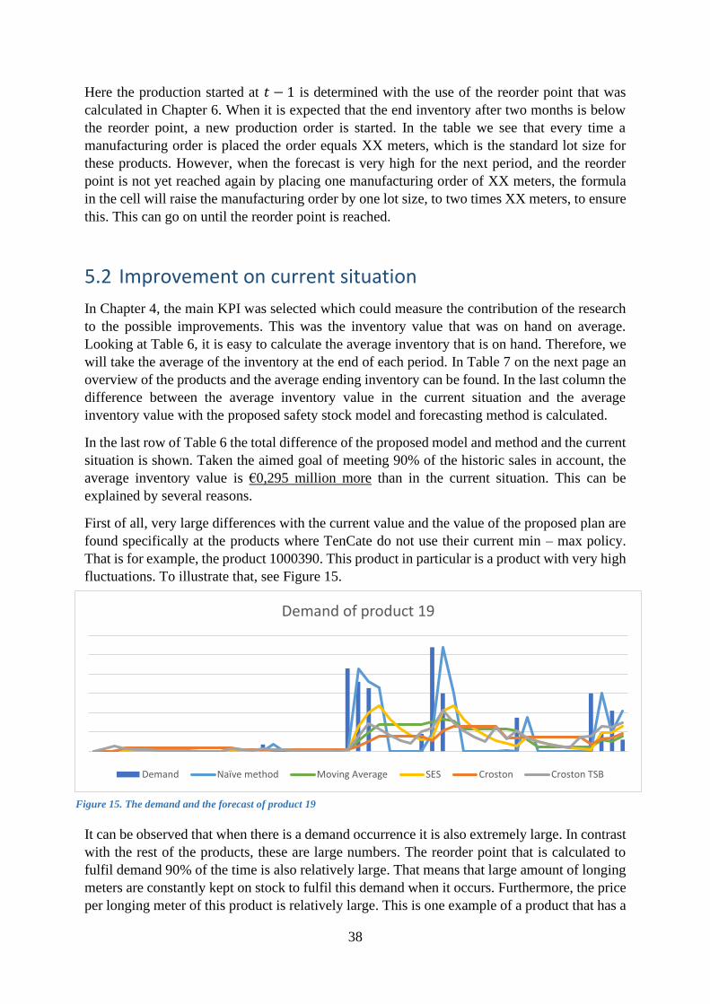
38

Here the production started at 𝑡 − 1 is determined with the use of the reorder point that was

calculated in Chapter 6. When it is expected that the end inventory after two months is below

the reorder point, a new production order is started. In the table we see that every time a

manufacturing order is placed the order equals XX meters, which is the standard lot size for

these products. However, when the forecast is very high for the next period, and the reorder

point is not yet reached again by placing one manufacturing order of XX meters, the formula

in the cell will raise the manufacturing order by one lot size, to two times XX meters, to ensure

this. This can go on until the reorder point is reached.

5.2 Improvement on current situation

In Chapter 4, the main KPI was selected which could measure the contribution of the research

to the possible improvements. This was the inventory value that was on hand on average.

Looking at Table 6, it is easy to calculate the average inventory that is on hand. Therefore, we

will take the average of the inventory at the end of each period. In Table 7 on the next page an

overview of the products and the average ending inventory can be found. In the last column the

difference between the average inventory value in the current situation and the average

inventory value with the proposed safety stock model and forecasting method is calculated.

In the last row of Table 6 the total difference of the proposed model and method and the current

situation is shown. Taken the aimed goal of meeting 90% of the historic sales in account, the

average inventory value is €0,295 million more than in the current situation. This can be

explained by several reasons.

First of all, very large differences with the current value and the value of the proposed plan are

found specifically at the products where TenCate do not use their current min – max policy.

That is for example, the product 1000390. This product in particular is a product with very high

fluctuations. To illustrate that, see Figure 15.

It can be observed that when there is a demand occurrence it is also extremely large. In contrast

with the rest of the products, these are large numbers. The reorder point that is calculated to

fulfil demand 90% of the time is also relatively large. That means that large amount of longing

meters are constantly kept on stock to fulfil this demand when it occurs. Furthermore, the price

per longing meter of this product is relatively large. This is one example of a product that has a

Demand of product 19

Demand Naïve method Moving Average SES Croston Croston TSB

Figure 15. The demand and the forecast of product 19

39

high reorder point for only a few demand occurrences. It can be seen in Appendix B that

TenCate itself does not have standard inventories of these products. That is because these

products are currently made by using an MTO-policy. However, in the proposed situation they

are treated as MTS-products. That is one reason why the inventory value is bigger, for this

product it is for example even €173.589 more inventory.

Table 7. Average inventory value with proposed safety stock model and forecasting method

Material

Number

Proposed average

end inventory

price/m Proposed average

inventory value

Difference with

current average

value

(current – proposed)

1 Intentionally left blank € -1.194,69

2 € 3.243,18

3 € -6.925,44

4 € -355,43

5 € -25.719,00

6 € -2.718,64

7 € 12.412,96

8 € -44.272,36

9 € -3.094,37

10 € 10.673,76

11 € -20.887,15

12 € -3.387,45

13 € 2.926,44

14 € 3.249,03

15 € 217,12

16 € -1.976,41

17 € -2.960,37

18 € 1.794,21

19 € -173.589,74

20 € -4.302,91

21 € 13.345,98

22 € 25.595,93

23 € -867,04

24 € -1.325,50

25 € -1.233,79

26 € -621,96

27 € -77.465,59

Total € 689.104 € -299.439

Besides that, there is also another reason why the average inventory of the proposed model and

method is higher than the current inventory value. That is because the data of the demand

occurrences is in fact only the sales that have occurred. Since customers sometimes accept a

delay in delivery time, the order becomes a backorder and is fulfilled in the next month and

sales will also occur in that month. However, it can also be a case of lost sales when a customer

needs a product at a specific time, but TenCate cannot deliver that on time, then the customer

40

can order the products at a competitor. When assuming that sometimes there are occurrences

of lost sales, it also means that sometimes a large order can be fulfilled from the inventory when

there is an accidental large stock kept. These are some of the outliers of the demand or sales

data. So, with the proposed safety stock model when the inventory is higher than in the current

situation, it could also be that occurrences of lost sales would then be fulfilled. So, when

attaining a service level of 90 percent, and thus having higher inventories it is possible that

more orders could have been fulfilled, however lost sales orders are not registered.

Lastly the desired service level is now set on 90 percent. This can be high for the business in

which TenCate operates. That means that it also includes fulfilling some outliers in the sales

data. That means, that when striving to attain the 90 percent service level, it is consciously taken

into account that these outliers should be fulfilled. Therefore, the reorder points are sometimes

higher than in the current situation. However, in the current situation these outliers were

fulfilled by an accidental high inventory of the product, or it could be that the order was placed

a long time before it was needed. Meaning that the planner could plan the manufacturing in

such a way that there is just enough inventory to satisfy that outlier.

5.3 Conclusion

In summary, the proposed safety stock model and the proposed forecasting method can be used

for the inventory management of TenCate. For some products the average inventory value goes

down in comparison to the current situation. However, with the new proposed model some

products should also have a higher reorder point and thus a larger average inventory.

41

6 CONCLUSIONS & RECOMMENDATIONS

6.1 Conclusions

This thesis presents a solution to the core problem. The core problem for the company was that

safety stock levels were not calculated. The main research question is:

“How can TenCate make a proper forecast and have an adequate inventory management in a

highly volatile market?”

To answer this question, several research questions were formulated. These were the guidelines

to make this thesis and tackle the core problem. The steps that were taken to come up with the

safety stock levels are the following:

- The current situation was analysed.

- The literature was studied to find out which safety stock models do exist and where they

differ on.

- Forecasting methods were compared quantitatively.

- The best safety stock model for TenCate was chosen.

- The variables for the safety stock model were determined, including the safety stock

levels.

Currently, TenCate makes use of minimum and maximum safety stock levels that are estimated

by the planner and not calculated. These safety stock levels can be calculated with a safety stock

model that is suitable for TenCate. During the research the best safety stock model was found

to be the (R, s, S)-model. For the selected products the best variables were calculated for each

of them, such as the reorder point and the safety stock level.

Another part of the research question covered the forecasting in a highly volatile market. For

that specific part a quantitative comparison was done between five different forecasting

methods. The forecasting method that was most appropriate for TenCate was the improved

Croston method by Teunter, Syntetos and Babai, or the Croston TSB method in short.

To measure the contribution of the research, a key performance indicator was selected. This

was the average inventory value. The new proposed way of forecasting and inventory

management unfortunately returned a higher average inventory value in a simulation. There are

several reasons why this is the case.

▪ The targeted service level that was set in this thesis could be high in the business of

TenCate.

▪ Some products that were investigated are not appropriate for a make-to-order policy.

▪ The data that was used was sales data and not actual demand data. Therefore, some

outliers in the sales could coincidentally be met by inventory on hand. That sales data

then becomes demand data. With the service level that was targeted, also these high

demand peeks should be met, which results in larger inventories on hand.

42

Besides the reasoning why the average inventory value was higher, other conclusions can be

drawn. The higher inventory value also does have an advantage. When having a higher

inventory value, it means that more inventory is laying on stock and therefore demand can be

met more often on time. That is good for the customer reputation. Next to that, orders that

became lost sales in the past, can be fulfilled more often with the new proposed method.

Retrieving the formula of the inventory turnover ratio from Chapter 1:

𝐼𝑛𝑣𝑒𝑛𝑡𝑜𝑟𝑦 𝑇𝑢𝑟𝑛𝑜𝑣𝑒𝑟 𝑅𝑎𝑡𝑖𝑜 = 𝐶𝑜𝑠𝑡 𝑜𝑓 𝐺𝑜𝑜𝑑𝑠 𝑆𝑜𝑙𝑑 ÷ 𝐴𝑣𝑒𝑟𝑎𝑔𝑒 𝐼𝑛𝑣𝑒𝑛𝑡𝑜𝑟𝑦

it can be retrieved that the costs of goods sold will then be raised by fulfilling demand more

often, and that subsequently will higher the inventory turnover ratio. However, due to the lack

of data on lost sales and backorders it cannot be retrieved how many times this would be the

case.

All in all, the core problem of safety stocks that were not calculated, is solved. That means that

the perceived problem, or starting problems, of the company are also solved. The company

experienced too many backorders and meanwhile they had a lot of inventories. As can be seen

in Table 7, some products need higher safety stocks, which would then probably be the products

that experience more backorders, and some products need less safety stock, which will reduce

the products that have too many inventory on stock.

Also, a solution is provided for a quantitative way of forecasting demand in a highly volatile

market. The main research question is therefore answered. Next to that, remarks are placed by

the provided solutions and proposed new way of inventory management in order to be useful

for the company.

6.2 Further research

Part of the discussion is the further research that can be executed after this thesis.

When looking at this thesis, still some more interesting results can be found by including the

capacity of the production hall. It was now assumed that there was no limit to the production,

however that is a simplification that maybe does change the planning and thus the reorder point

and safety stock levels. By incorporating the capacity of the production hall, the lead time

calculations become more accurate. Which will lead to calculations with proposed solutions

that are closer to reality.

Another thing than can be investigated deeper is the classification of the different products. In

this research they were separated by the probability of a demand occurrence, however, there are

also a lot of different other options to divide the products into groups. One of these options that

can be interesting for TenCate is making use of the ABC-analysis. The ABC-analysis makes

use of a product classification based on the percentage of one product on the total revenue. In

short, this means that a small percent of the (top-selling) items is responsible for a large amount

of the sales. In Figure 16 this is represented by the green rectangle. This rectangle are the A-

class products. In this example, around 15% of the products is responsible for 70% of the sales.

The orange rectangle represents B-class products, 20% are represents 20% of the sales. Lastly

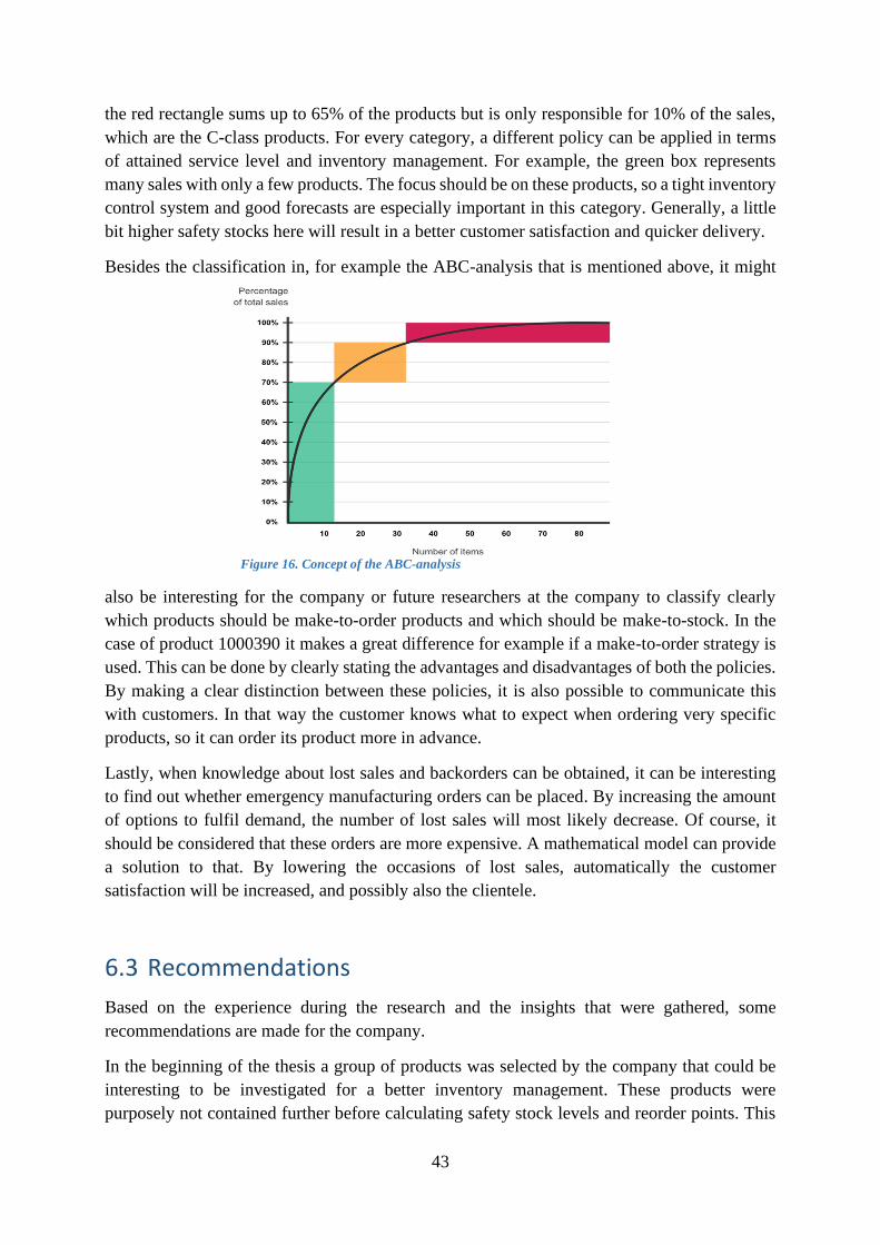
43

the red rectangle sums up to 65% of the products but is only responsible for 10% of the sales,

which are the C-class products. For every category, a different policy can be applied in terms

of attained service level and inventory management. For example, the green box represents

many sales with only a few products. The focus should be on these products, so a tight inventory

control system and good forecasts are especially important in this category. Generally, a little

bit higher safety stocks here will result in a better customer satisfaction and quicker delivery.

Besides the classification in, for example the ABC-analysis that is mentioned above, it might

also be interesting for the company or future researchers at the company to classify clearly

which products should be make-to-order products and which should be make-to-stock. In the

case of product 1000390 it makes a great difference for example if a make-to-order strategy is

used. This can be done by clearly stating the advantages and disadvantages of both the policies.

By making a clear distinction between these policies, it is also possible to communicate this

with customers. In that way the customer knows what to expect when ordering very specific

products, so it can order its product more in advance.

Lastly, when knowledge about lost sales and backorders can be obtained, it can be interesting

to find out whether emergency manufacturing orders can be placed. By increasing the amount

of options to fulfil demand, the number of lost sales will most likely decrease. Of course, it

should be considered that these orders are more expensive. A mathematical model can provide

a solution to that. By lowering the occasions of lost sales, automatically the customer

satisfaction will be increased, and possibly also the clientele.

6.3 Recommendations

Based on the experience during the research and the insights that were gathered, some

recommendations are made for the company.

In the beginning of the thesis a group of products was selected by the company that could be

interesting to be investigated for a better inventory management. These products were

purposely not contained further before calculating safety stock levels and reorder points. This

Figure 16. Concept of the ABC-analysis

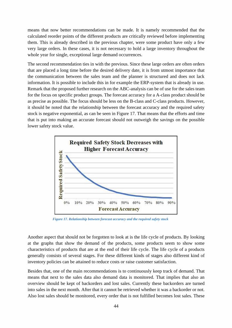
44

means that now better recommendations can be made. It is namely recommended that the

calculated reorder points of the different products are critically reviewed before implementing

them. This is already described in the previous chapter, were some product have only a few

very large orders. In these cases, it is not necessary to hold a large inventory throughout the

whole year for single, exceptional large demand occurrences.

The second recommendation ties in with the previous. Since these large orders are often orders

that are placed a long time before the desired delivery date, it is from utmost importance that

the communication between the sales team and the planner is structured and does not lack

information. It is possible to include this in for example the ERP-system that is already in use.

Remark that the proposed further research on the ABC-analysis can be of use for the sales team

for the focus on specific product groups. The forecast accuracy for a A-class product should be

as precise as possible. The focus should be less on the B-class and C-class products. However,

it should be noted that the relationship between the forecast accuracy and the required safety

stock is negative exponential, as can be seen in Figure 17. That means that the efforts and time

that is put into making an accurate forecast should not outweigh the savings on the possible

lower safety stock value.

Another aspect that should not be forgotten to look at is the life cycle of products. By looking

at the graphs that show the demand of the products, some products seem to show some

characteristics of products that are at the end of their life cycle. The life cycle of a products

generally consists of several stages. For these different kinds of stages also different kind of

inventory policies can be attained to reduce costs or raise customer satisfaction.

Besides that, one of the main recommendations is to continuously keep track of demand. That

means that next to the sales data also demand data is monitored. That implies that also an

overview should be kept of backorders and lost sales. Currently these backorders are turned

into sales in the next month. After that it cannot be retrieved whether it was a backorder or not.

Also lost sales should be monitored, every order that is not fulfilled becomes lost sales. These

Figure 17. Relationship between forecast accuracy and the required safety stock

45

numbers can also be interesting to use in further research. For example, when there is a lot of

lost sales for one specific product, it can be rewarding if there is kept more inventory of that

product. In that way higher sales can be generated.

Lastly it would be of great value for the company when there is a continuous view on important

KPIs for the planner. Currently there is a small dashboard build in Excel with only a few graphs.

However, a dashboard with specific KPIs per business process would give far more insights.

These KPIs include for example the inventory turnover and the average inventory value. This

can be presented in a dashboard, which could also be useful for the management.

46

7 BIBLIOGRAPHY

Aardal, K., Jonsson, Ö., & Jönsson, H. (1989). Optimal Inventory Policies with Service-Level

Constraints. Journal of the Operational Research Society 40(1), 65-73.

Beutel, A.-L., & Minner, S. (2012). Safety stock planning under causal demand forecasting.

International Journal of Production Economics 140(2), 637-645.

Bijulal, D., Venkateswaran, J., & Hemachandra, N. (2011). Service levels, system cost and

stability of production-inventory control systems. International Journal of Prpduction

Research 49(23), 7085-7105.

Braglia, M., Castellano, D., & Frosolini, M. (2014). Safety stock management in single

vendor-single buyer problem under VMI with consignment stock agreement.

International Journal of Production Economics 154, 16-31.

Brooks, R., & Gray, B. (2001). History of Forecdasters: An assessment of the semi-annual

U.S. Treasury Bond Yield Forecast Survey as Reported in The Wall STreet Journal.

Working Paper NO. 03-06-1, The University of Alabama.

Chu, Y.-F., & Lin, W.-C. (2004). A Study Of Inventory Model Based On Order Quantity And

Lead Time As Decision Variables—Demand Frequency And Quantities

Corresponding Poisson And Normal Distribution. Journal of the Chinese Institute of

Industrial Engineers 21(4), 384-394.

Cooper, D. R., & Schindler, P. S. (2014). Research in Business. In Business Research

Methods, Twelfth Edition (pp. 21-24). New York: McGraw-Hill/Irwin.

Croston, J. (1972). Forecasting and Stock Control for Intermittent Demands. Operational

Research Quarterly Vol. 23, 289-303.

Dissartation, L. (n.d.). Fundamentals: principles of research ethics. Retrieved from Laerd

dissertation: http://dissertation.laerd.com/principles-of-research-ethics.php

Grubbström, R., & Wikner, J. (1996). Inventory trigger control policies developed in terms of

control theory. International Journal of Production Economics 45(1-3), 397-406.

Heerkens, H., & Winden, A. v. (2012). Geen probleem: een aanpak voor alle bedrijfskundige

vragen en mysteries. Nieuwegein: Van Winden Communicatie.

Hottenhuis, W. (2019). Finding the right type of research for my bachelor assignment. Essay,

University of Twente, BMS, Enschede.

Hsueh, C.-F. (2011). An inventory control model with consideration of remanufacturing and

product life cycle. International Journal of Production Economics 133(2), 645-652.

47

Kang, C. W., Ullah, M., & Sarkar, B. (2017). Optimum ordering policy for an imperfect

single-stage manufacturing system with safety stock and planned backorder.

International Journal of Advanced Manufacturing Technology, 109-120.

Klosterhalfen, S., & Minner, S. (2010). Safety stock optimisation in distribution systems: A

comparison of two competing approaches. International Journal of Logistics Research

and Applications 13(2), 99-120.

Kok, A. (1985). Approximations for a lost-sales production/inventory control model with

service lvel constraints. Journal of Management Science 31(6), 729-737.

Li, L. (1992). THE ROLE OF INVENTORY IN DELIVERY-TIME COMPETITION.

Management Science, Vol. 38, No. 2, 182-197.

Moinzadeh, Kamran, Schmidt, & P, C. (1991). (S - 1, S) inventory system with emergency

orders. Operations Research 39(2), 308-321.

Pink, D. (2009). Drive: the surprising truth about what motivates us. Journal of community &

applied social psychology.

Poel, I. v., & Royakkers, L. (2011). Ethics, Technology, and Engineering: An Introduction.

Porras, E., & Dekker, R. (2008). An inventory control system for spare parts at a refinery: An

empirical comparison of different re-order point methods. European Journal of

Operational Research 184(1), 101-132.

Ruiz-Torres, A., & Mahmoodi, F. (2010). Safety stock determination based on parametric

lead time and demand information. International Journal of Production Research

48(10), 2841-2857.

Sani, B., & Kingsman, B. (1997). Selecting the best periodic inventory controldemand

forecasting methods for low demand items. Journal of the Operational Research

Society 48(7), 700-713.

Sarkar, B., Sana, S., & Chaudhuri, K. (2010). Optimal reliability, production lotsize and

safety stock: An economic manufacturing quantity model. International Journal of

Management Science and Engineering Management 5(3), 192-202.

Sellitto, M. (2018). Lead-time, inventory, and safety stock calculation in job-shop

manufacturing. Acta Polytechnica, 395-401.

Tempelmeier, H. (2013). A multi-level inventory system with a make-to-order supplier.

International Journal of Production Research 51(23-24), 6880-6890.

Teunter, R., Syntetos, A., & Babai, M. (2011). Intermittent demand: Linking forecasting to

inventory obsolescence. European Journal of Operational Research.

Tukey, J. (2011). Exploratrory Data Analysis. Exploratory Data Analysis SAGE, 533.

48

Van Donselaar, K., & Broekmeulen, R. (2013). Determination of safety stocks in a lost sales

inventory system with periodic review, positive lead-time, lot-sizing and a target fill

rate. International Journal of Production Economics 143(2), 440-448.

Vandeput, N. (2018). Croston model. In DATA SCIENCE FOR SUPPLY CHAIN FORECAST.

Winston, W. L. (2004). Operations Research Applications and Algorithms, fourth edition.

Curt Hinrichs.

Yadollahi, E., Aghezzaf, E.-H., & Raa, B. (2016). A Statistical Comparison of Two Safety

Stock Replenishment Mechanisms in a Cyclic Stochastic IRP. IFAC-PapersOnLine,

1508-1513.

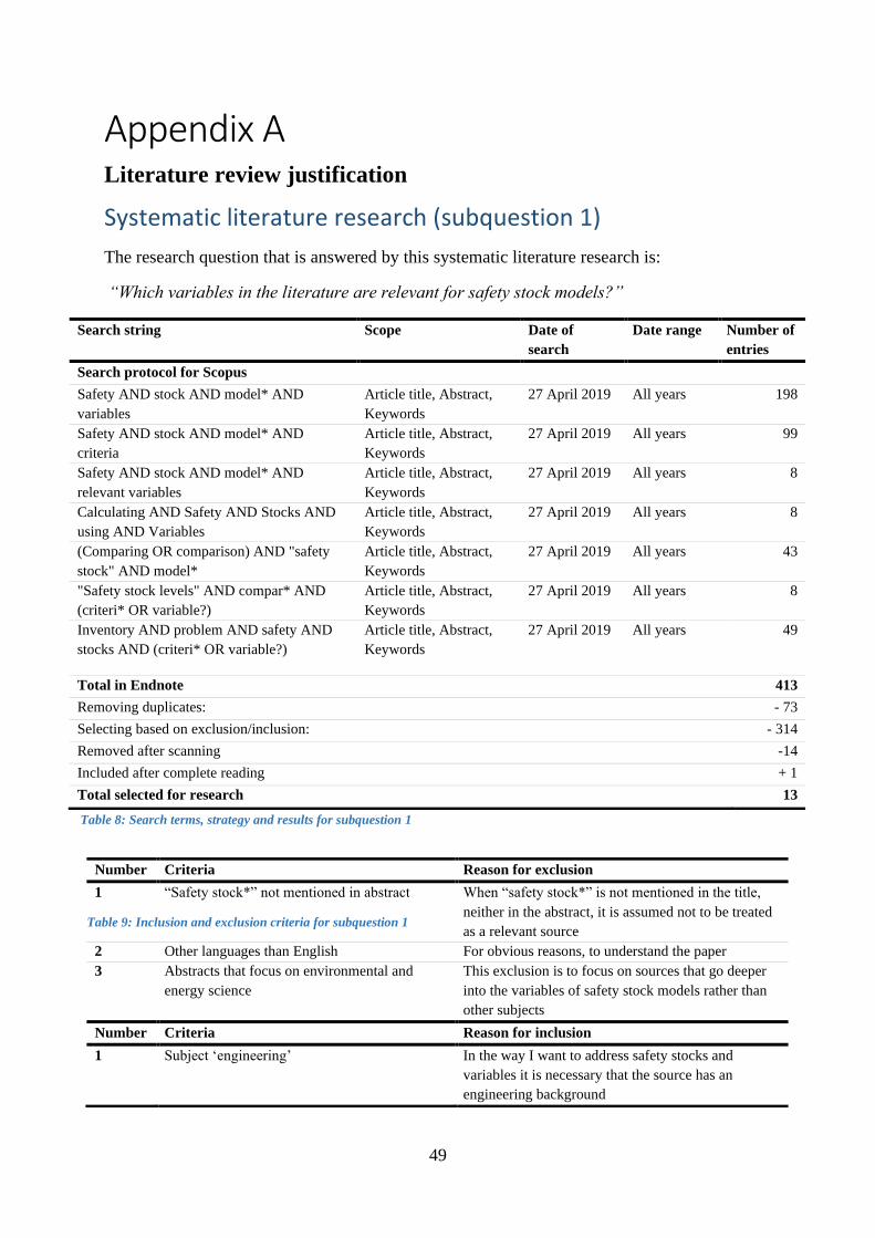
49

Appendix A Literature review justification

Systematic literature research (subquestion 1)

The research question that is answered by this systematic literature research is:

“Which variables in the literature are relevant for safety stock models?”

Search string Scope Date of

search

Date range Number of

entries

Search protocol for Scopus

Safety AND stock AND model* AND

variables

Article title, Abstract,

Keywords

27 April 2019 All years 198

Safety AND stock AND model* AND

criteria

Article title, Abstract,

Keywords

27 April 2019 All years 99

Safety AND stock AND model* AND

relevant variables

Article title, Abstract,

Keywords

27 April 2019 All years 8

Calculating AND Safety AND Stocks AND

using AND Variables

Article title, Abstract,

Keywords

27 April 2019 All years 8

(Comparing OR comparison) AND "safety

stock" AND model*

Article title, Abstract,

Keywords

27 April 2019 All years 43

"Safety stock levels" AND compar* AND

(criteri* OR variable?)

Article title, Abstract,

Keywords

27 April 2019 All years 8

Inventory AND problem AND safety AND

stocks AND (criteri* OR variable?)

Article title, Abstract,

Keywords

27 April 2019 All years 49

Total in Endnote 413

Removing duplicates: - 73

Selecting based on exclusion/inclusion: - 314

Removed after scanning -14

Included after complete reading + 1

Total selected for research 13

Table 8: Search terms, strategy and results for subquestion 1

Number Criteria Reason for exclusion

1 “Safety stock*” not mentioned in abstract When “safety stock*” is not mentioned in the title,

neither in the abstract, it is assumed not to be treated

as a relevant source

2 Other languages than English For obvious reasons, to understand the paper

3 Abstracts that focus on environmental and

energy science

This exclusion is to focus on sources that go deeper

into the variables of safety stock models rather than

other subjects

Number Criteria Reason for inclusion

1 Subject ‘engineering’ In the way I want to address safety stocks and

variables it is necessary that the source has an

engineering background

Table 9: Inclusion and exclusion criteria for subquestion 1

50

# Article / Book Authors

(year)

Important concepts About Special for

1

Optimum ordering policy for

an imperfect single-stage

manufacturing system with

safety stock and planned

backorder

(Kang, Ullah, &

Sarkar, 2017)

Lot sizes, demand stability,

planned backorders, total

costs

Minimizing the

total average cost

function by

making a

mathematical

model

Manufacturer

2

Lead-time, inventory, and

safety stock calculation in

job-shop manufacturing

(Sellitto, 2018) Lead-time, uncertainty lot

size, average inventory, total

costs, demand rate

Describing a

method for

calculating lead-

time, inventory

and safety stock

Job-shop

manufacturer

3

A Statistical Comparison of

Two Safety Stock

Replenishment Mechanisms

in a Cyclic Stochastic IRP

(Yadollahi,

Aghezzaf, & Raa,

2016)

Backorders, service level,

average inventory, demand

rate

Two policies on

safety stock

replenishments:

Fair-share and

Ratio

Cyclic

inventory

routing

problems

4

Safety stock management in

single vendor-single buyer

problem under VMI with

consignment stock

agreement

(Braglia,

Castellano, &

Frosolini, 2014)

Demand, holding costs,

service level, number of

stockouts, total costs.

Minimum cost

solution

-

5

A multi-level inventory

system with a make-to-order

supplier

(Tempelmeier,

2013)

Lead time, holding costs,

processing costs, service

level

Minimum cost

solution

Factory,

warehouse and

DCs

6

Safety stock planning under

causal demand forecasting

(Beutel & Minner,

2012)

Uncertainty of demand,

service level, total costs

Not parametric

demand and

attaining service

level.

Causal demand

7

Service levels, system cost

and stability of production-

inventory control systems

(Bijulal,

Venkateswaran, &

Hemachandra,

2011)

Stability against demand

fluctuations, service level,

average system costs

Comparison

between different

inventory systems

-

8

An inventory control model

with consideration of

remanufacturing and

product life cycle

(Hsueh, 2011) Production lot size, demand

rate, lead time, holding costs

Different models

for different

phases of product

life cycle

-

9

Safety stock optimisation in

distribution systems: A

comparison of two

competing approaches

(Klosterhalfen &

Minner, 2010)

Service level, holding costs,

total costs, demand per period

with standard deviation

Stochastic-service

approach versus

internal service

level

determination

10

Optimal reliability,

production lotsize and safety

stock: An economic

manufacturing quantity

model

(Sarkar, Sana, &

Chaudhuri, 2010)

(Demand) reliability, average

cost, production lotsize

Smallest average

integrated costs

Production

facilities

11 Safety stock determination

based on parametric lead

(Ruiz-Torres &

Mahmoodi, 2010)

Demand variability, total

costs

Inventory model

that accounts for

Production

facilities

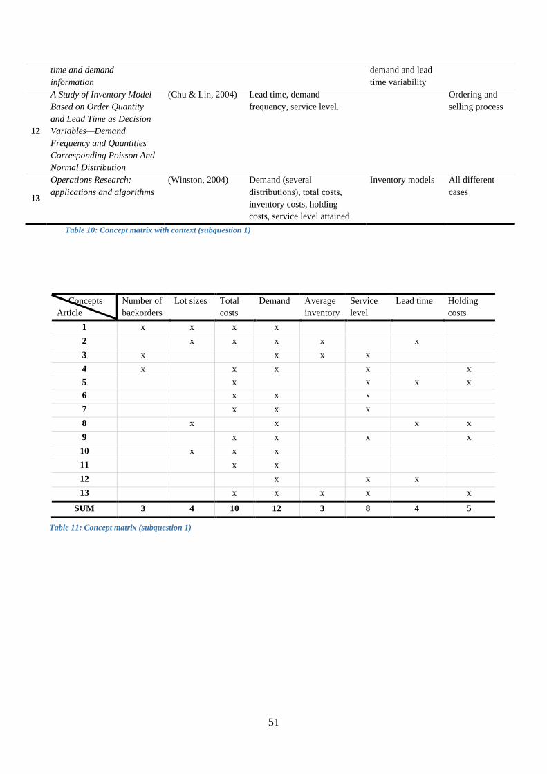
51

time and demand

information

demand and lead

time variability

12

A Study of Inventory Model

Based on Order Quantity

and Lead Time as Decision

Variables—Demand

Frequency and Quantities

Corresponding Poisson And

Normal Distribution

(Chu & Lin, 2004) Lead time, demand

frequency, service level.

Ordering and

selling process

13

Operations Research:

applications and algorithms

(Winston, 2004) Demand (several

distributions), total costs,

inventory costs, holding

costs, service level attained

Inventory models All different

cases

Table 10: Concept matrix with context (subquestion 1)

Concepts

Article

Number of

backorders

Lot sizes Total

costs

Demand Average

inventory

Service

level

Lead time Holding

costs

1 x x x x

2 x x x x x

3 x x x x

4 x x x x x

5 x x x x

6 x x x

7 x x x

8 x x x x

9 x x x x

10 x x x

11 x x

12 x x x

13 x x x x x

SUM 3 4 10 12 3 8 4 5

Table 11: Concept matrix (subquestion 1)

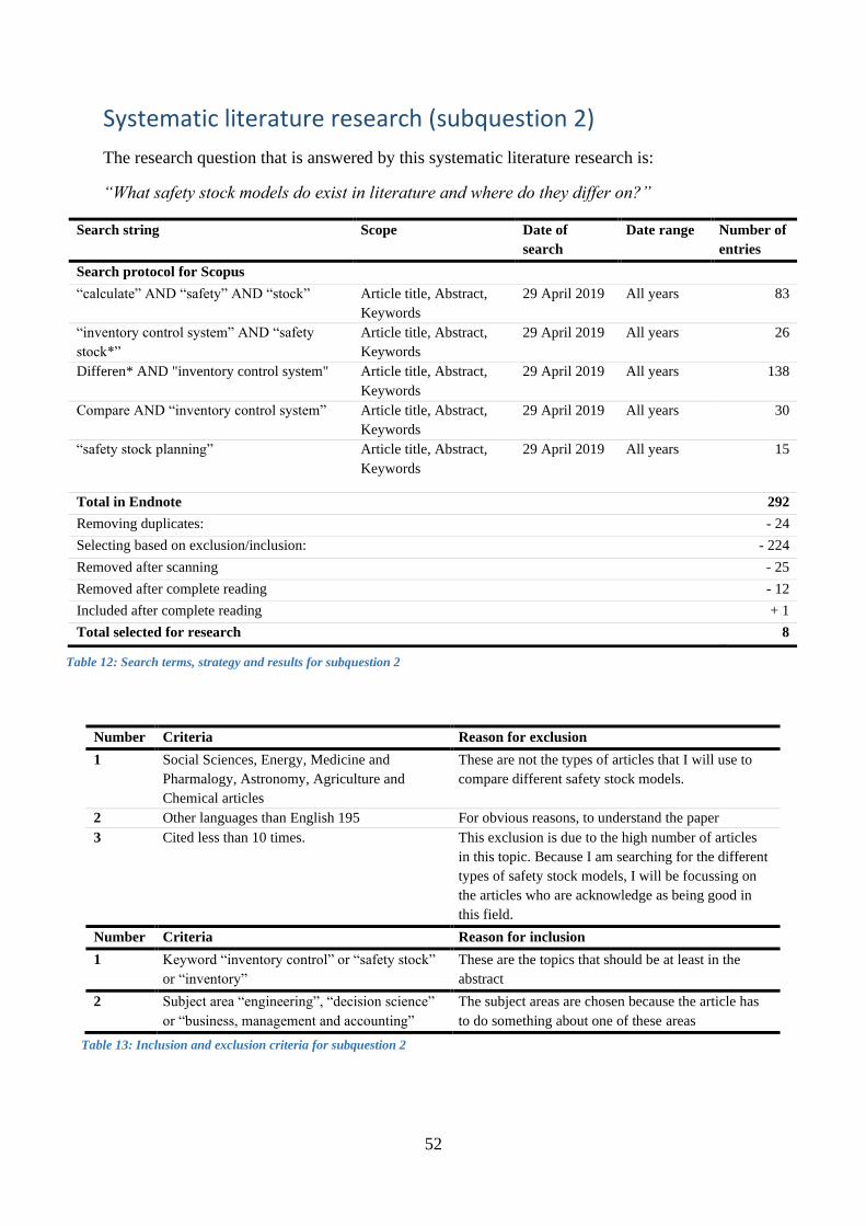
52

Systematic literature research (subquestion 2)

The research question that is answered by this systematic literature research is:

“What safety stock models do exist in literature and where do they differ on?”

Search string Scope Date of

search

Date range Number of

entries

Search protocol for Scopus

“calculate” AND “safety” AND “stock” Article title, Abstract,

Keywords

29 April 2019 All years 83

“inventory control system” AND “safety

stock*”

Article title, Abstract,

Keywords

29 April 2019 All years 26

Differen* AND "inventory control system" Article title, Abstract,

Keywords

29 April 2019 All years 138

Compare AND “inventory control system” Article title, Abstract,

Keywords

29 April 2019 All years 30

“safety stock planning” Article title, Abstract,

Keywords

29 April 2019 All years 15

Total in Endnote 292

Removing duplicates: - 24

Selecting based on exclusion/inclusion: - 224

Removed after scanning - 25

Removed after complete reading - 12

Included after complete reading + 1

Total selected for research 8

Table 12: Search terms, strategy and results for subquestion 2

Number Criteria Reason for exclusion

1 Social Sciences, Energy, Medicine and

Pharmalogy, Astronomy, Agriculture and

Chemical articles

These are not the types of articles that I will use to

compare different safety stock models.

2 Other languages than English 195 For obvious reasons, to understand the paper

3 Cited less than 10 times. This exclusion is due to the high number of articles

in this topic. Because I am searching for the different

types of safety stock models, I will be focussing on

the articles who are acknowledge as being good in

this field.

Number Criteria Reason for inclusion

1 Keyword “inventory control” or “safety stock”

or “inventory”

These are the topics that should be at least in the

abstract

2 Subject area “engineering”, “decision science”

or “business, management and accounting”

The subject areas are chosen because the article has

to do something about one of these areas

Table 13: Inclusion and exclusion criteria for subquestion 2

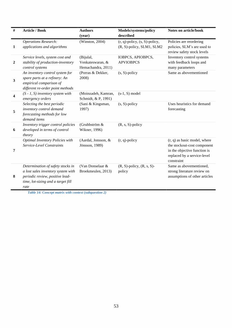
53

# Article / Book Authors

(year)

Models/systems/policy

described

Notes on article/book

1

Operations Research:

applications and algorithms

(Winston, 2004) (r, q)-policy, (s, S)-policy,

(R, S)-policy, SLM1, SLM2

Policies are reordering

policies, SLM’s are used to

review safety stock levels

2

Service levels, system cost and

stability of production-inventory

control systems

(Bijulal,

Venkateswaran, &

Hemachandra, 2011)

IOBPCS, APIOBPCS,

APVIOBPCS

Inventory control systems

with feedback loops and

many parameters

3

An inventory control system for

spare parts at a refinery: An

empirical comparison of

different re-order point methods

(Porras & Dekker,

2008)

(s, S)-policy Same as abovementioned

4 (S - 1, S) inventory system with

emergency orders

(Moinzadeh, Kamran,

Schmidt, & P, 1991)

(s-1, S) model

5

Selecting the best periodic

inventory control demand

forecasting methods for low

demand items

(Sani & Kingsman,

1997)

(s, S)-policy Uses heuristics for demand

forecasting

6

Inventory trigger control policies

developed in terms of control

theory

(Grubbström &

Wikner, 1996)

(R, s, S)-policy

7

Optimal Inventory Policies with

Service-Level Constraints

(Aardal, Jonsson, &

Jönsson, 1989)

(r, q)-policy (r, q) as basic model, where

the stockout-cost component

in the objective function is

replaced by a service-level

constraint

8

Determination of safety stocks in

a lost sales inventory system with

periodic review, positive lead-

time, lot-sizing and a target fill

rate

(Van Donselaar &

Broekmeulen, 2013)

(R, S)-policy, (R, s, S)-

policy

Same as abovementioned,

strong literature review on

assumptions of other articles

Table 14: Concept matrix with context (subquestion 2)

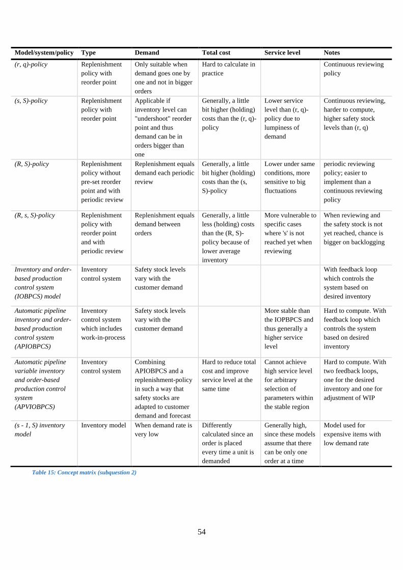
54

Model/system/policy Type Demand Total cost Service level Notes

(r, q)-policy Replenishment

policy with

reorder point

Only suitable when

demand goes one by

one and not in bigger

orders

Hard to calculate in

practice

Continuous reviewing

policy

(s, S)-policy Replenishment

policy with

reorder point

Applicable if

inventory level can

"undershoot" reorder

point and thus

demand can be in

orders bigger than

one

Generally, a little

bit higher (holding)

costs than the (r, q)-

policy

Lower service

level than (r, q)-

policy due to

lumpiness of

demand

Continuous reviewing,

harder to compute,

higher safety stock

levels than (r, q)

(R, S)-policy Replenishment

policy without

pre-set reorder

point and with

periodic review

Replenishment equals

demand each periodic

review

Generally, a little

bit higher (holding)

costs than the (s,

S)-policy

Lower under same

conditions, more

sensitive to big

fluctuations

periodic reviewing

policy; easier to

implement than a

continuous reviewing

policy

(R, s, S)-policy Replenishment

policy with

reorder point

and with

periodic review

Replenishment equals

demand between

orders

Generally, a little

less (holding) costs

than the (R, S)-

policy because of

lower average

inventory

More vulnerable to

specific cases

where 's' is not

reached yet when

reviewing

When reviewing and

the safety stock is not

yet reached, chance is

bigger on backlogging

Inventory and order-

based production

control system

(IOBPCS) model

Inventory

control system

Safety stock levels

vary with the

customer demand

With feedback loop

which controls the

system based on

desired inventory

Automatic pipeline

inventory and order-

based production

control system

(APIOBPCS)

Inventory

control system

which includes

work-in-process

Safety stock levels

vary with the

customer demand

More stable than

the IOPBPCS and

thus generally a

higher service

level

Hard to compute. With

feedback loop which

controls the system

based on desired

inventory

Automatic pipeline

variable inventory

and order-based

production control

system

(APVIOBPCS)

Inventory

control system

Combining

APIOBPCS and a

replenishment-policy

in such a way that

safety stocks are

adapted to customer

demand and forecast

Hard to reduce total

cost and improve

service level at the

same time

Cannot achieve

high service level

for arbitrary

selection of

parameters within

the stable region

Hard to compute. With

two feedback loops,

one for the desired

inventory and one for

adjustment of WIP

(s - 1, S) inventory

model

Inventory model When demand rate is

very low

Differently

calculated since an

order is placed

every time a unit is

demanded

Generally high,

since these models

assume that there

can be only one

order at a time

Model used for

expensive items with

low demand rate

Table 15: Concept matrix (subquestion 2)

55

Appendix B Current average inventory value INTENTIONALLY LEFT BLANK DUE TO CONFIDENTIALLITY

56

Appendix C All products with demand and probability of demand occurrence INTENTIONALLY LEFT BLANK DUE TO CONFIDENTIALLITY

57

Appendix D Mean Squared Error for different forecasting methods INTENTIONALLY LEFT BLANK DUE TO CONFIDENTIALLITY