Improved learning of I2C distance and accelerating the

neighborhood search for image classification

Zhengxiang Wanga, Yiqun Hub, Liang-Tien Chiaa

aCenter for Multimedia and Network Technology, School of Computer EngineeringNanyang Technological University, 639798, Singapore

bSchool of Computer Science and Software EngineeringThe University of Western Australia, Australia

wang0460@ntu.edu.sg, yiqun.hu@uwa.edu.au, asltchia@ntu.edu.sg

Abstract

Image-To-Class (I2C) distance is a novel measure for image classification andhas successfully handled datasets with large intra-class variances. However,due to the lack of a training phase, the performance of this distance is easilyaffected by irrelevant local features that may hurt the classification accuracy.Besides, the success of this I2C distance relies heavily on the large number oflocal features in the training set, which requires expensive computation costfor classifying test images. On the other hand, if there are small number oflocal features in the training set, it may result in poor performance.

In this paper, we propose a distance learning method to improve the clas-sification accuracy of this I2C distance as well as two strategies for accelerat-ing its NN search. We first propose a large margin optimization framework tolearn the I2C distance function, which is modeled as a weighted combinationof the distance from every local feature in an image to its nearest neighbor(NN) in a candidate class. We learn these weights associated with local fea-tures in the training set by constraining the optimization such that the I2Cdistance from image to its belonging class should be less than that to anyother class. We evaluate the proposed method on several publicly availableimage datasets and show that the performance of I2C distance for classi-fication can significantly be improved by learning a weighted I2C distancefunction. To improve the computation cost, we also propose two methodsbased on spatial division and hubness score to accelerate the NN search,which is able to largely reduce the on-line testing time while still preservingor even achieving a better classification accuracy.

Preprint submitted to Pattern Recognition December 28, 2010

Keywords: Image-To-Class Distance, Distance Learning, ImageClassification, Nearest Neighbor Classification

1. Introduction

Image classification is an active research topic in computer vision commu-nity due to the large intra-class variances and ambiguities of images. Manyefforts have been investigated for dealing with this problem. Among recentworks, nearest-neighbor (NN) based methods [1–8] have been attractive forhandling the classification task due to its simple implementation and effectiveperformance. While most studies focus on measuring the distance betweenimages, e.g. learned local Image-To-Image (I2I) distance function [2, 3], a newNN based Image-To-Class (I2C) distance is proposed by Boiman et al. [1] intheir Naive-Bayes Nearest-Neighbor (NBNN) method, which achieves state-of-the-art performance in several challenging datasets despite the simplicityof its algorithm. Compared to previous works using NN based methods, thisnew distance similarity measure directly deals with each image representedby a set of patch based local features, e.g. SIFT features [9], while most pre-vious studies require quantizing these features into a fixed-length vector forrepresentation, which may lose the discriminate information from the origi-nal image. The training feature set of each class is constructed by gatheringfeatures in every training image belonging to that class. The I2C distancefrom a test image to a candidate class is formulated as the sum of Euclideandistance between each feature in this test image and its NN feature searchedfrom the training feature set of the candidate class. This is also different frommost previous studies that only measure the distance between images. Theyattribute the success of NBNN to the avoidance of descriptor quantizationand the use of I2C distance instead of I2I distance, and they have shown thatdescriptor quantization and I2I distance lead to significant degradation forclassification.

The effectiveness of this I2C distance attracts many recent studies. Forexample, Huang et al. [10] applied it in face and human gait recognition,Wang et al. [11] learn a distance metric for this I2C distance, Behmo et al.[12] learn an optimal NBNN by hinge-loss minimization to further enhanceits generalization ability, etc.

However, in the formulation of this I2C distance, each local feature in thetraining set is given equal importance. This makes the I2C distance sensitive

2

Test Image

.

.

.

Find NN for

each feature Weight learnt during the

training procedure and

associated with each

feature

Weighted I2C distance

Feature Collection

of Class 1

Feature Collection

of Class N

ArgMin (Dist)

Class 1

Beach

Feature extracted

from patches

Dist of Class 1

Dist of Class 2

Dist of Class 3

Dist of Class N

.

.

.

Dist of Class 1

Dist of Class 2

Dist of Class 3

Dist of Class N

.

.

.

I2C distance

After Weight

Figure 1: The whole procedure for classifying a test image. The I2C distances to differentclasses are denoted as different length of blue bars for expressing the relative size.

to irrelevant features, which are useless for measuring the distance and mayhurt the classification accuracy. Besides, the performance of this I2C distancerelies heavily on the large number of local features in the training set, whichrequires expensive computation cost during the NN search when classifyingtest images. On the other hand, a small training feature set may result inpoor performance, although it requires less time for the NN search.

In this paper, we propose a novel NN based classification method forlearning a weighted I2C distance. For each local feature in the training set,we learn a weight associated with it during the training phase, thus decreasingthe impacts of irrelevant features that are useless for measuring the distance.These weights are learned by formulating a weighted I2C distance function inthe training phase, which is achieved by constraining the weighted I2C dis-tance to the belonging class to be the shortest for each training image amongits I2C distances to all classes. We adopt the large margin idea in Fromeet al. [3] and formulate the triplet constraint in our optimization problemthat the I2C distance for each training image to its belonging class should beless than the distance to any other class with a large margin. Therefore, ourmethod avoids the shortcomings of both non-parametric methods and mostlearning-based methods involving I2I distance and descriptor quantization.This leads to a better classification accuracy than NBNN or those learning-based methods while requiring relatively smaller number of local features in

3

the training set.With the weighted I2C distance from a test image to each candidate class,

we predict the class label of this test image using a simple nearest-neighborclassifier as in [1], which selects the class with the shortest I2C distance as itspredicted label. The whole procedure of classifying the test image is shownin Figure 1. First a set of local features are extracted from a given testimage (denoted as crosses with different colors). Then for each feature, itsNN feature in each class’s feature set is searched (denoted as crosses withthe same color). The weighted I2C distance to each class is formulated asthe sum of Euclidean distance between each individual feature and its NNfeature in the class weighted by its associated weight, and the class with theshortest I2C distance is selected as the predicted class.

The main computational bottleneck in I2C distance is the NN featuresearch due to the large number of features in the training feature set for eachclass. In most real world applications the training set is extremely large,which makes the NN search time consuming. Our training cost for learningthe weight would be negligible compared to this heavy NN search. So inthis paper we propose two methods for accelerating the NN search, whichmake the I2C distance more practical for real world problems. These twomethods reduce the candidate features set for the NN search from differentaspects. The first method uses spatial division to split the image into severalspatial subregions and restrict each feature to find its NN only in the samespatial subregion, while the second method ranks all local features in thetraining set by hubness score [13] and removes those features with low hubnessscore. Both methods are able to accelerate the NN search significantly whilemaintaining or even achieving better classification accuracy.

This paper is an extension work of our published conference paper in[14]. The main extension work includes: 1. We provide a more completedescription on the technique detail. 2. We propose two new methods foraccelerating the NN search due to the heavy computation cost of the NNsearch. 3. We add five new publicly available datasets in the experimentsection to validate our proposed methods.

The paper is organized as follows. In Section 2 we present a large marginoptimization framework for learning the weight. Two NN search accelera-tion methods are present in Section 3. We validate our approach throughexperiment in Section 4. Finally, the conclusion is written in Section 5.

4

Image Xi

Class c

k,cf

Image Xi

Class c

j,ifk,ck,c wf ¬2

k,cj,i ff -2

k,cj,ik,c ffw -×

j,if

Original I2C distance Weighted I2C distance

Figure 2: The original unweighted I2C distance in NBNN (left) and our proposed weightedI2C distance (right).

2. Learning Image-To-Class Distance

In this section, we propose a large margin optimization framework toconstruct a weighted I2C distance by learning the weight associated with eachfeature in the training set. These features are extracted from patches aroundeach keypoint and represented by some local descriptor such as SIFT [9]. Wefirst explain some notations for clarity. Let Fi = {fi,1, fi,2, . . . , fi,mi

} denotelocal features belonging to an image Xi, where mi represents the number offeatures in Xi and each feature is denoted as fi,j ∈ Rd,∀j ∈ {1, . . . , mi}.The feature set of each class c is composed of features from all trainingimages belonging to that class and is denoted as Fc = {fc,1, fc,2, . . . , fc,mc}.Similarly, here mc represents the number of features in class c. The originalunweighted I2C distance from image Xi to a class c is formulated as the sumof L2 distance (Euclidean distance) between every feature fi,j in Xi and itsNN feature in class c denoted as fc,k, which is shown in the left part of Figure2. Here the NN feature fc,k is searched over the feature set of class c that hasthe shortest L2 distance to feature fi,j in image Xi and the distance betweenthem is denoted as dj,k. This NN search is time consuming when the trainingfeature set is large, so we will discuss some acceleration methods in Section3. The formulation of this I2C distance is given as:

Dist(Xi, c) =

mi∑j=1

‖ fi,j − fc,k ‖2=

mi∑j=1

dj,k (1)

Wherek = arg min

k′={1,...,mc}‖ fi,j − fc,k′ ‖2 (2)

5

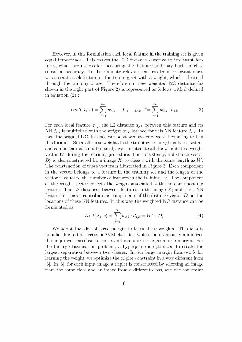
However, in this formulation each local feature in the training set is givenequal importance. This makes the I2C distance sensitive to irrelevant fea-tures, which are useless for measuring the distance and may hurt the clas-sification accuracy. To discriminate relevant features from irrelevant ones,we associate each feature in the training set with a weight, which is learnedthrough the training phase. Therefore our new weighted I2C distance (asshown in the right part of Figure 2) is represented as follows with k definedin equation (2) :

Dist(Xi, c) =

mi∑j=1

wc,k· ‖ fi,j − fc,k ‖2=

mi∑j=1

wc,k · dj,k (3)

For each local feature fi,j, the L2 distance dj,k between this feature and itsNN fc,k is multiplied with the weight wc,k learned for this NN feature fc,k. Infact, the original I2C distance can be viewed as every weight equating to 1 inthis formula. Since all these weights in the training set are globally consistentand can be learned simultaneously, we concatenate all the weights to a weightvector W during the learning procedure. For consistency, a distance vectorDc

i is also constructed from image Xi to class c with the same length as W .The construction of these vectors is illustrated in Figure 3. Each componentin the vector belongs to a feature in the training set and the length of thevector is equal to the number of features in the training set. The componentof the weight vector reflects the weight associated with the correspondingfeature. The L2 distances between features in the image Xi and their NNfeatures in class c contribute as components of the distance vector Dc

i at thelocations of these NN features. In this way the weighted I2C distance can beformulated as:

Dist(Xi, c) =

mi∑j=1

wc,k · dj,k = W T ·Dci (4)

We adopt the idea of large margin to learn these weights. This idea ispopular due to its success in SVM classifier, which simultaneously minimizesthe empirical classification error and maximizes the geometric margin. Forthe binary classification problem, a hyperplane is optimized to create thelargest separation between two classes. In our large margin framework forlearning the weight, we optimize the triplet constraint in a way different from[3]. In [3], for each input image a triplet is constructed by selecting an imagefrom the same class and an image from a different class, and the constraint

6

fi,1

.

.

.

d1,1

0

d2,3

0

0

0

0

0

d3,9

0

.

.

.

Image Xi

x1 x2

x3

x1

x2

x3

.

.

.

wc,1

wc,2

wc,3

wc,4

wc,5

wc,6

wc,7

wc,8

wc,9

wc,10

.

.

.

Wc

iD

Class c

fi,2

fi,3

d1,1

d2,3

d3,9

fc,1

fc,3

fc,9

Figure 3: The construction of distance vector Dci and weight vector W . The I2C distance

between image Xi and class c is represented by the distance vector Dci . x1, x2, x3 represent

the training images in class c. The crosses in each image represent features extracted forthat image. For the test image Xi, its local features fi,1, fi,2, fi,3 find their NN fc,1,fc,3,fc,9

in class c. d1,1, d2,3 and d3,9 are the L2 distances between features in Xi and their NNfeatures in class c, and they contribute as components of Dc

i at the locations of their NNfeatures. In this way the weighted I2C distance can be formulated as WT ·Dc

i .

is formulated that the I2I distance between images in the same class shouldbe less than that in different classes with a margin. Besides the limitationincurred by I2I distance as described in [1], this triplet formulating methodwill cause too many triplet constraints in the distance learning, especiallywhen there are large number of training images in each class. However, byusing I2C distance, we construct our triplet for each input image just byselecting two classes, one as positive class that the image belongs to, and theother from any other class as negative class, hereby reducing the number oftriplet constraints significantly. Our triplet constraint is therefore formulatedby keeping the I2C distance to the positive class to be less than that to thenegative class with a margin. This is illustrated in Figure 4. For each inputimage Xi, the triplet with positive class p and negative class n should beconstrained as:

W T · (Dni −Dp

i ) ≥ 1− ξipn (5)

Here the slack variable ξipn is used for soft-margin as in the standard SVMform.

We formulate our large margin optimization problem in the form similarto SVM. Since the initial weight of each feature is 1 as in the original I2C

7

Image Xi

Positive Class p Negative Class nass p N

NN feature

L2 distance

Optimization Constraint:

Feature

Weighted I2C

distance

kp,f

kj,d

ji,f

k,jj k,p

p

i

T dwDW ×=× åk,jj k,n

n

i

T dwDW ×=× å

( ) ipn

p

i

n

i

T 1DDW x-³-×

Figure 4: The triplet constraint for distance learning. For an image Xi, its I2C distanceto the positive class p should be less than that to the negative class n with a margin.

distance, we regularize the learned weights according to a prior weight vectorW0, whose elements are all equal to 1. This is to penalize those weightsthat are too far away from this prior in the optimization problem and keepconsistency between training and testing phase. The optimization problemis given as:

arg minW,ξ

1

2||W −W0||2 + C

∑i,p,n

ξipn (6)

s.t.∀ i, p, n : W · (Dni −Dp

i ) ≥ 1− ξipn

ξipn ≥ 0

∀ k : W (k) ≥ 0

Here the parameter C controls the trade-off between the regularization anderror terms as in SVM optimization problem. Each element of the opti-mizing weight vector is enforced to be non-negative as distances are alwaysnon-negative. For a dataset with Nc classes, the number of triplet constraintsfor each training image is Nc − 1 since there are Nc − 1 different negativeclasses, and the total number of triplet constraints in the optimization prob-lem should be (Nc−1)×Nc×Ntr, where Ntr stands for the number of training

8

images in each class. This is a significant reduction compared to the numberof triplets in I2I distance [3], which needs O(N2

c × N3tr) triplets for learning

the weight. Such reduction on the number of triplets will result in a fasterspeed during the weight updating procedure.

We solve the optimization problem of equation (6) in the dual form usingthe method in [3] as:

arg maxα,µ

−1

2||

∑i,p,n

αipn ·Qipn + µ||2 +∑ipn

αipn (7)

− [∑ipn

αijk ·Qipn + µ] ·W0

s.t. ∀ i, p, n : 0 ≤ αipn ≤ C

∀ j : µ(j) ≥ 0

Where Qipn = (Dni −Dp

i ) for simplicity. This dual form is solved by iterativelyupdating the dual variable α and µ alternatively. Each time we update theα variables that violate the Karush Kuhn Tucker (KKT) [15] conditions bytaking the derivative of equation (7) with respect to α and then update µ toensure the positiveness of weight vector W in each iteration. The updatedformula of α and µ is given as:

αipn = [{1−∑

{i′,p′,n′}6={i,p,n}αi′p′n′〈Qi′p′n′ ·Qipn〉 −

〈(µ + W0) ·Qipn〉}/ ‖ Qipn ‖2][0,C]

µ = max{0,−∑i,p,n

αipn ·Qipn −W0} (8)

And the KKT conditions are:

αipn = 0 ⇒ W ·Qipn ≥ 1

0 < αipn < C ⇒ W ·Qipn = 1

αipn = C ⇒ W ·Qipn ≤ 1 (9)

The operation of [f(x)][0,C] is to clip the value of f(x) in the region [0, C],and {i′, p′, n′} represent any triplet in constraint set that is different from{i, p, n}. Since the optimization problem is convex, this objective functionis guaranteed to reach the global minimum after iterative updating. The

9

number of α variable is equal to the number of triplet constraints, which ismuch less than that in the I2I distance framework that was mentioned before.After convergence, the weight vector W in the primer form can be calculatedby:

W =∑i,p,n

αi,p,n ·Qi,p,n + µ + W0 (10)

As all weights are optimized simultaneously in the weight vector, this consis-tency will ensure global ranking of the weighted I2C distances to all classes.

3. Efficiency Improvement

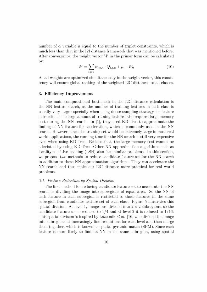
The main computational bottleneck in the I2C distance calculation isthe NN feature search, as the number of training features in each class isusually very large especially when using dense sampling strategy for featureextraction. The large amount of training features also requires large memorycost during the NN search. In [1], they used KD-Tree to approximate thefinding of NN feature for acceleration, which is commonly used in the NNsearch. However, since the training set would be extremely large in most realworld applications, the running time for the NN search is still very expensiveeven when using KD-Tree. Besides that, the large memory cost cannot bealleviated by using KD-Tree. Other NN approximation algorithms such aslocality-sensitive hashing (LSH) also face similar problems. In this section,we propose two methods to reduce candidate feature set for the NN searchin addition to these NN approximation algorithms. They can accelerate theNN search and thus make our I2C distance more practical for real worldproblems.

3.1. Feature Reduction by Spatial Division

The first method for reducing candidate feature set to accelerate the NNsearch is dividing the image into subregions of equal area. So the NN ofeach feature in each subregion is restricted to those features in the samesubregion from candidate feature set of each class. Figure 5 illustrates thisspatial division. At level 1, images are divided into 2× 2 subregions, so thecandidate feature set is reduced to 1/4 and at level 2 it is reduced to 1/16.This spatial division is inspired by Lazebnik et al. [16] who divided the imageinto subregions at increasingly fine resolutions for each level and then mergethem together, which is known as spatial pyramid match (SPM). Since eachfeature is more likely to find its NN in the same subregion, using spatial

10

Figure 5: The I2C NN feature search with spatial division. We adopt the idea of spatialpyramid by restricting the NN of each feature in the same subregion at each spatial level.

division to reduce the candidate set will preserve the classification accuracyof weighted I2C distance while accelerating the NN search. For scene imagesthat usually have geometric structures and classes that manifest commonspatial layout, this spatial division will not only accelerate the NN search,but also improve classification accuracy, as it can reduce the rate of falseNN match. Even for datasets with less spatial aligned images, this spatialdivision can still work. This is because the NN of each local feature in a testimage is searched over every training image in the same subregion and it isless likely that none of the training images contain the object in the samesubregion as in the test image.

Besides accelerating the NN search for improving efficiency, the spatialdivision can also be used to further improve the classification accuracy. Thiscan be achieved by adding the weighted I2C distances from different spatiallevels to formulate the I2C distance with SPM as shown in Figure 5, whichis analogous to the spatial pyramid [16] and pyramid match [17]. Althoughusing spatial division at a single spatial level can accelerate the NN search,the SPM of combining multiple spatial levels for improving the classificationaccuracy requires additional running time. Note that the spatial subregionscannot be divided too finely, as it will make the NN search too sensitive to thespatial layout and increase the number of false matches. For the experimentsin this paper, we use spatial division for learning I2C distance only at spatiallevel 1 (2× 2 subregions) and level 2 (4× 4 subregions).

11

3.2. Feature Reduction by Hubness Score

Spatial division is a simple but effective method for reducing candidatefeature set. However, this method does not remove any feature in the trainingset and therefore still requires large memory cost during the NN search . Forsuch situation, we develop another method which explores the hubness offeatures in candidate set for feature reduction. This is inspired by the workof [13], which measured data points using hubness score and explored itsimportance in many NN problems. Specifically, the hubness of a data pointis reflecting the number of times this point is matched by other points astheir NN. A hubness score is therefore introduced to measure the hubnessof each data point. For those points with high occurrences as NN points byothers, they should have high hubness score and thus are recognized as hubpoints.

In our problem where the weighted I2C distance is used for classification,we define a new hubness score for measuring the importance of each feature(here a data point is represented as a feature) in candidate set. Those unim-portant features with low hubness scores are removed for improvement inspeed. Inspired by the triplet in our learning framework which is composedof positive and negative classes, the counting of occurrence as matched byother features should also be split into positive and negative parts, since theoccurrence of being matched by features in the belonging class plays a differ-ent role to that in other classes. Intuitively, we would want to remove thosefeatures frequently matched by features from other class while less likely tobe matched from the belonging class. Let Np(x) denotes the number of timesa feature is matched by other features from the belonging class, which wealso call positive match. Similarly, we denote the negative match Nn(x) asthe number of times a feature is matched by features from other classes. Wedefine the hubness score of each feature x by:

h(x) =Np(x)

Nn(x)(11)

For all features in the training set, we rank them in the order of descendinghubness score, and only preserve features with higher hubness score. Otherfeatures are removed permanently and no longer put into the candidate fea-ture set. We only learn the weights for these preserved features and use themfor NN match during the testing phase.

12

3.3. Discussion

We discuss the advantages and disadvantages of the two proposed meth-ods for accelerating the NN search. The first method uses spatial division toreduce candidate set for each feature in a test image during the NN search.Since determining which subregion a feature in test image belongs to is sim-ply calculated by its pixel location, the selection of reduced candidate featureset for the NN search will require little time during the testing phase. Forgeometric structured images, this method performs even better than with-out spatial division. However, this method does not remove any feature inthe training set, therefore it still requires large memory cost during the NNsearch. The number of weights for learning is not reduced either, which mayresult in a long running time during learning when the training set is verylarge.

The second method does not have the above mentioned problems. Sincethe features with low hubness scores are removed permanently after rankingall training features, it can reduce the memory cost during the NN searchin the testing phase. It can also speed up the weight learning procedure,as lesser number of weights is required for learning. However, unlike spa-tial division that can improve classification accuracy for structured images,this method may lose some accuracy when most of the training features arereduced. In addition, every feature in the training set needs to count itspositive and negative match for calculating hubness score, which increasesthe computation cost during the training phase, although faster NN searchspeed in the testing phase is gained.

To achieve the best efficiency, both methods can be combined togetherfor the task of NN search during the I2C distance calculation.

4. Experiment

4.1. Datasets and Setup

We evaluate our proposed method on five publicly available datasets:Scene-15, Sports, Corel, Caltech 101 and Caltech 256 datasets. We describethem briefly as follows:

• Scene-15: Scene dataset consists of 15 scene categories, among which8 were originally collected by Oliva et al. [18], 5 added by Li et al.[19] and 2 from Lazebnik et al. [16]. Each class has about 200 to400 images, and the average image size is around 300 × 250 pixels.

13

Following [16], we randomly select 100 images per class for training,and test on the rest. The average of each per-class accuracy is reportedfor evaluation.

• Sports: Sports event dataset is firstly introduced in [20], consisting of8 sports event categories. The number of images in each class rangesfrom 137 to 250, so we follow [20] to select 70 and 60 images per class fortraining and test respectively. Since images in this dataset are usuallyvery large, they are first resized such that the largest x/y dimension is500.

• Corel: Corel dataset contains 10 scene categories published by CorelCorporation. Each class contains 100 images, and we follow [21] toseparate them randomly into two subsets of equal size to form thetraining and test set. All the images are of the size 384 × 256 or 256× 384.

• Caltech 101: Caltech 101 dataset is a large scale dataset containing101 categories [22]. The number of images in each class varies fromabout 30 to 800. This dataset is more challenging due to the largenumber of classes and intra-class variance. Following the widely usedmeasurement by the community we randomly select 15 images per classfor training. For testing, we also select 15 images for each class andreport the mean accuracy.

• Caltech 256: Caltech 256 dataset [23] is even larger than Caltech101. Each class contains at least 80 images. The total of 256 categoriesmake this dataset much more challenging than the other four datasets.We use this dataset to validate the scalability of our methods. In theexperiment we randomly select 15 images per class for training and 25different images per class for test.

Since the training and test set are selected randomly, we repeat eachdataset for 5 times and report the average result. For feature extraction, weuse dense sampling strategy and SIFT features [9] as our descriptor, which areextracted over every 8 pixels for all datasets. Although this feature extractionis simple and even discard color information, encouraging performance canbe achieved. For the parameter C in our learning problem, we empiricallyfix it to 1 throughout the experiment. We name our method as LI2C, shortfor Learning Image-To-Class distance.

14

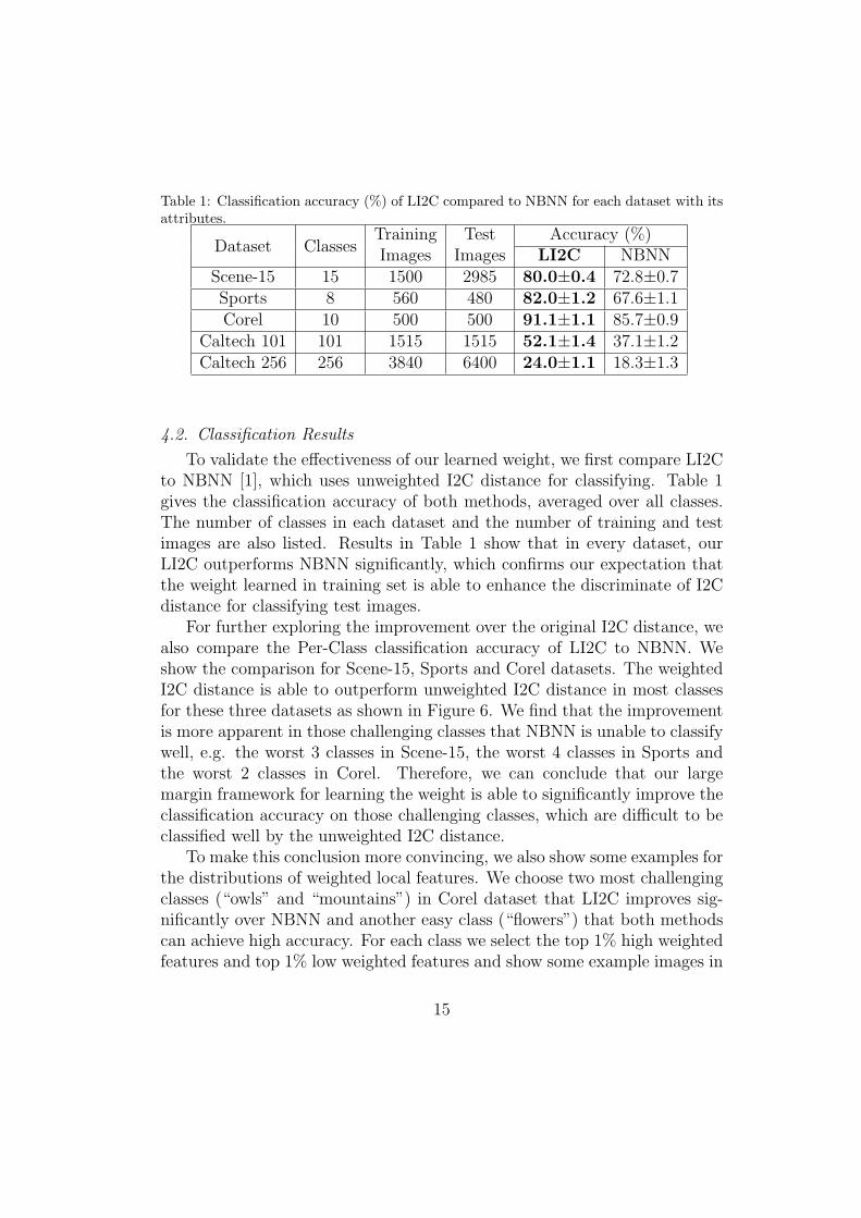
Table 1: Classification accuracy (%) of LI2C compared to NBNN for each dataset with itsattributes.

Training Test Accuracy (%)Dataset Classes

Images Images LI2C NBNNScene-15 15 1500 2985 80.0±0.4 72.8±0.7Sports 8 560 480 82.0±1.2 67.6±1.1Corel 10 500 500 91.1±1.1 85.7±0.9

Caltech 101 101 1515 1515 52.1±1.4 37.1±1.2Caltech 256 256 3840 6400 24.0±1.1 18.3±1.3

4.2. Classification Results

To validate the effectiveness of our learned weight, we first compare LI2Cto NBNN [1], which uses unweighted I2C distance for classifying. Table 1gives the classification accuracy of both methods, averaged over all classes.The number of classes in each dataset and the number of training and testimages are also listed. Results in Table 1 show that in every dataset, ourLI2C outperforms NBNN significantly, which confirms our expectation thatthe weight learned in training set is able to enhance the discriminate of I2Cdistance for classifying test images.

For further exploring the improvement over the original I2C distance, wealso compare the Per-Class classification accuracy of LI2C to NBNN. Weshow the comparison for Scene-15, Sports and Corel datasets. The weightedI2C distance is able to outperform unweighted I2C distance in most classesfor these three datasets as shown in Figure 6. We find that the improvementis more apparent in those challenging classes that NBNN is unable to classifywell, e.g. the worst 3 classes in Scene-15, the worst 4 classes in Sports andthe worst 2 classes in Corel. Therefore, we can conclude that our largemargin framework for learning the weight is able to significantly improve theclassification accuracy on those challenging classes, which are difficult to beclassified well by the unweighted I2C distance.

To make this conclusion more convincing, we also show some examples forthe distributions of weighted local features. We choose two most challengingclasses (“owls” and “mountains”) in Corel dataset that LI2C improves sig-nificantly over NBNN and another easy class (“flowers”) that both methodscan achieve high accuracy. For each class we select the top 1% high weightedfeatures and top 1% low weighted features and show some example images in

15

0 0.2 0.4 0.6 0.8 1

store

industrial

bedroom

living room

kitchen

street

mountain

open country

highway

coast

inside city

tall building

forest

office

suburb

Scene 15

LI2CNBNN

0 0.2 0.4 0.6 0.8 1

boccesnowboarding

sailingrowing

polorock climbing

croquetbadminton

Sports

LI2CNBNN

0 0.2 0.4 0.6 0.8 1

mountainsowls

beachbuildings

skiingtigers

elephantsflowers

foodhorses

Corel

LI2CNBNN

Figure 6: Per-Class classification accuracy on Scene-15, Sports and Corel datasets forcomparing our method with NBNN.

Figure 7. We can see that in the two challenging classes most high weightedfeatures are locate on the object, while the location of low weighted featuresare more arbitrary, i.e. either on the object or the background. As in LI2Cthose features with high weight are given more importance, the weighted I2Cdistance is able to largely improve the classification accuracy over the origi-nal unweighted distance. However, in the class of “flowers”, both high andlow weighted features are difficult to be distinguished from either the objector background. As both weighted and unweighted I2C distances can easilyclassify images in this class, this distribution shows that features located onboth the object and background in this class are useful for the classification.Some predicted examples in this dataset are also shown in Figure 8. In thetop row, both methods are able to correctly classify these images. In themiddle row, images are wrongly classified by NBNN. However, after learn-ing the weight, they can be correctly classified by our LI2C. In the bottomrow, we also show images that are unable to be correctly classified even afterlearning the weight. We can see that some of these images are difficult to beclassified as they has less connection to their ground truth labels.

Compared to the published result of NBNN [1] on Caltech 101 and Caltech256 datasets, our implementation of NBNN achieves lower result than their

16

Owls

Mountains Flowers

Figure 7: Distributions of local features with high weight (red) and low weight (blue) forclasses of “owls”, “mountains” and “flowers” in Corel dataset.

best reported performance. We notice that they have used multiple scalesand more densely sampled features in their experiment, which is about 20times more than the number of features in our experiment. This shows thatthe performance of I2C distance without training phase relies heavily on thelarge number of complex features, which require heavy computation cost forthe NN search. In contrast, we use simpler and smaller number of features inour experiment and therefore achieve a much lower result for NBNN, whichproves that using small number of features result in poor performance forI2C distance without training phase. However, by learning the weight usingour proposed method, the performance of I2C distance can be significantlyimproved using the same, small number of features. In addition, even us-ing a large number of local features in the training set same as that in [1],we are unable to reproduce the result reported in [1]. We guess this maybe due to the different parameter settings in the SIFT feature extractionstage. However, the result of our implemented NBNN is comparable to thatin [11]. Since both methods use the same feature descriptor as input in ourexperiment, the comparison of our method with NBNN is fair. This experi-ment also shows that our large margin framework for learning the weight is

17

Ground Truth &

LI2C& NBNNskiing owls mountains flowers beach buildings tigers

Ground Truth

& LI2Cskiing owls owls owls mountains mountains flowers buildings

NBNN building tigers flowers food skiing elephants food elephants

Ground Truth skiing owls mountains beach buildings buildings food

LI2C owls tigers buildings buildings food owls tigers

NBNN food tigers food buildings food food tigers

Figure 8: Predicted examples in Corel dataset. Images in the top row are correctlyclassified by both LI2C and NBNN. The middle row shows images that are correctlyclassified by LI2C but wrongly classified by NBNN, and images in the bottom row arewrongly classified by either LI2C or NBNN.

capable of dealing with large-scale datasets, while the computation cost ofweight updating procedure in training is nearly negligible compared to theNN search in the I2C distance calculation as mentioned before.

4.3. Results on Spatial Division

Next we analyze the performance of LI2C as well as NBNN at differentspatial levels. Table 2 shows the results of both methods from level 0 to level 2as well as their combinations (SPM). Compared to level 0, the classificationaccuracies of both methods are improved at either spatial level 1 or level2. This proves that spatial division is able to not only accelerate the NNsearch, but also improve the classification accuracy. Since images in theSports dataset do not have such common spatial layout like that in sceneconstraint structures of the other datasets, but still gain improvement whenusing spatial division, we suggest that the spatial division is a useful strategyto help improve I2C distance in most real-world images. We also notice

18

Table 2: Classification accuracy (%) of LI2C compared to NBNN on different spatiallevels as well as SPM for Scene-15, Sports, Corel, Caltech 101 and Caltech 256 datasets. L0denotes level 0 of 1×1 subregions, L1 denotes level 1 of 2×2 subregions and L2 denotes level2 of 4×4 subregions. SPM combines three spatial levels and achieves the best accuracy,while the accuracy of spatial levels at L1 and L2 is better than L0.

LI2C (%) NBNN (%)Dataset L0 L1 L2 SPM L0 L1 L2 SPMScene-15 80.0 82.2 81.7 83.8 72.8 75.6 77.6 78.7Sports 82.0 83.5 84.0 84.1 67.6 71.3 71.2 71.4Corel 91.1 91.2 91.6 92.2 85.7 87.4 87.3 88.2

Caltech 101 52.1 58.1 62.1 66.7 37.4 43.6 48.1 50.4Caltech 256 24.0 25.5 29.2 30.2 18.3 20.0 21.0 22.2

that the largest improvement by spatial division is achieved in Caltech 101dataset, where the performances of both methods at level 1 are improvedover 6% compared to level 0 and further improved about 4% at level 2. Thismay be because that objects in most images of Caltech 101 dataset are oftenlocated at the center, so spatial division is able to maintain the commonspatial layout in each subregion and reduce the rate of false NN match.

Since SPM combines the I2C distances of all spatial levels, it achieves thebest classification accuracy in each dataset as shown in Table 2. However,SPM requires calculating the I2C distance and learning weight for LI2C ateach spatial level, so its computation cost is the sum of each spatial level andthus very expensive. Since the improvement of SPM is limited compared tosingle spatial level in these datasets, using only spatial division at level 1 orlevel 2 for classification is a better strategy when efficiency is the primaryissue. For example, the Caltech 256 dataset contains much more images andclasses than the others, so using spatial division at level 2 to learn its I2Cdistance is faster while its accuracy is close to that using SPM.

Although spatial division and SPM is able to improve the classificationperformances of both LI2C and NBNN, it should be emphasized that bylearning the weight for each training feature, our LI2C is more discrimina-tive than the unweighted I2C distance in NBNN in every spatial level andits combination, which again validate the effectiveness of our large marginframework for learning the weight.

19

Figure 9: Comparing the classification accuracy of LI2C to NBNN for Scene-15, Sportsand Corel datasets with various percentages of preserved training features in the trainingset.

4.4. Results on Hubness Score

The result of spatial division is encouraging for reducing the candidatefeature set during the NN search. However, a large number of features inthe training set are still stored in memory during the testing phase, becausefeatures in different subregions are required to be matched by features in thecorresponding subregions for each test image. Such large number of trainingfeatures not only occupy large memory space, but also require substantialcomputation cost for learning the weight associated with each feature. Theseproblems can be overcome by our second method for improving the efficiency.This new method reduces the training features by the use of hubness score.

20

Figure 10: Comparing the classification accuracy of LI2C to NBNN for Caltech 101 inspatial level 2 with various percentages of preserved training features in the training set.

To evaluate the effectiveness of this method, we compare the performancesof the training set with different sizes of preserved features. Here the amountof improvement on efficiency is represented by the percentage of preservedtraining features to the original, since less number of preserved features needless computation cost for the NN search and achieve better improvementon efficiency. Figure 9 shows the results of both LI2C and NBNN withpercentages of preserved training features ranging from 1% to 100% for Scene-15, Sports and Corel datasets. In all the three datasets, the accuracy reducedby our LI2C method is nearly negligible even when only 5% training featuresare preserved, but this reduction starts to become obvious when the preservedtraining features are reduced from 5% to 1%. However, massive reductionof training features will not allow NBNN to maintain satisfactory result,as its accuracy drops quickly in every dataset. This result indicates thatthe performance of NBNN relies heavily on the size of candidate trainingset, while our method is able to maintain the classification accuracy whenthere are only a small number of training features due to the effectivenessof learned weight. It should be emphasized that this method for featurereduction not only accelerates the NN search, but also speeds up weightlearning and requires less memory space.

We also evaluate the performance of combining both spatial division andhubness score. We use Caltech 101 dataset in spatial level 2 for this ex-periment with percentages of preserved features ranging from 1% to 100%.Results on both LI2C and NBNN are reported in Figure 10. Although only

21

Table 3: The average running time for weight learning and NN search of each image.(s=second, h=hour)

Weight Learning NN SearchScene-15 381s 155sSports 171s 270sCorel 74s 52s

Caltech 101 2151s 78sCaltech 256 3.5h 239s

15 images in each class are used for training in this dataset, which are muchless than the training sets in the previous three datasets, we can see that theclassification accuracy of our LI2C method is still close to the original untilthe percentage of preserved training features drops to below 10%, whereasthe accuracy of NBNN drops much faster compared to LI2C.

4.5. Computation analysis

We also show the computation cost of our learning method as well asthe accelerated NN search using our proposed two strategies. The averagerunning time for updating the weight using our large margin optimizationare shown in Table 3, where the running time for the NN search of eachimage without acceleration are also list as comparing. All of the experimentsare running on Intel x86 Xeon CPU E7320@2.13GHz. We can see thatin Scene-15, Sports and Corel datasets, due to the small number of classes,the weight learning procedure runs quickly and requires little computationcost. With the increased number of classes, more triplet constraints and moreweights are required to be updated. Therefore the running time for updatingthe weight on Caltech 101 and 256 datasets are increased. However, suchtraining cost is nearly negligible compared to the heavy computation cost forthe NN search. As Table 3 shows, it requires about 1 to 4 minutes for the NNsearch of only one image. This means for a dataset like Caltech 101, whichcontains 1515 test images, the total running time for the NN search is about32 hours. For the largest dataset of Caltech 256, which contains 6400 testimages, the running time is increased to 17 days. Such large computationcost makes the I2C distance impractical for large scale dataset.

However, with our proposed acceleration method, the running time forthe NN search can be significantly reduced. Taking Caltech 101 dataset as

22

Table 4: The average running time for the NN search of each image on different spatialdivision level and various percentages of preserved training features in the training set.(second)

Percentage of remaining training set1% 2% 5% 10% 15% 20% 25% 30% 40% 50% 100%

L0 1.9 2.8 5.2 9.0 12.8 16.8 20.8 24.8 30.4 33.1 78.0L1 1.4 1.8 2.7 3.6 4.5 5.5 6.5 7.6 9.4 11.4 24.7L2 1.6 2.2 3.3 4.3 5.1 5.6 6.1 6.6 7.3 7.9 12.1

example, using spatial division at level 2, the running time is reduced to12.1 seconds as shown in Table 4. By combining both spatial division andhubness score, the computation cost can be further reduced. As Figure 10in previous subsection shows, the classification accuracy of preserving 10%training features on spatial level 2 is comparable to the original for our LI2C.However, the computation cost is reduced to 4.3 seconds per image as shownin Table 4. So the total running time for the NN search of the whole test setis only 1.8 hours, which would make the I2C distance practical for applyingto large scale dataset.

4.6. Comparing to Previous Results

We also compare our method with recent published results on thesedatasets. All the results are summarized in Table 5. The best classifica-tion accuracy in our experiment is achieved by combining LI2C with SPM ineach dataset. Although we use single local feature in our experiment and donot even consider color information, our result is able to achieve state-of-the-art performance in most of these datasets. Specifically, in Scene-15 dataset,our result is able to outperform most of previous methods [16, 25, 26, 28].The current state-of-the-art performance for this dataset is around 84%[29, 27, 24]. However, we find that the best result among these resultsreported in [29] use multi-scale and densely sampled keypoints for featureextraction as well as multiple feature combination, which is much too com-plex, while our method uses single local feature but is still comparable tomost methods. Similar comparison is in Sports dataset, where our methodis significantly outperform [20, 31] and is comparable to [29]. For Corel, Cal-tech 101 and Caltech 256 datasets, our method is also able to outperformmost other methods that report their results recently.

23

Table 5: Comparing to recently published results for classification accuracy (%).Dataset Method Accuracy (%)

Ours 83.8Lazebnik et al. [16] 81.4

Liu et al. [24] 83.3Rasiwasia et al. [25] 72.2

Scene-15 van Gemert et al. [26] 76.5Bosch et al. [27] 83.7Yang et al. [28] 80.3Wu et al. [29] 84.1

Zhou et al. [30] 83.5Ours 84.1

Li et al. [20] 73.4Sports

Wu et al. [31] 78.5Wu et al. [29] 84.2

Ours 92.2Corel Lu et al. [32] 77.9

Lu et al. [21] 90.0Ours 66.7

Yang et al. [28] 67.0Caltech 101 Wang et al. [33] 65.4

Wu et al. [29] 65.2Gu et al. [34] 65.0

Ours 30.2Caltech 256 Yang et al. [28] 27.7

Griffin et al. [23] 28.3

24

5. Conclusion and Future Work

In this paper, we introduced a novel method for nearest-neighbor classi-fication by learning weighted Image-To-Class distance function. We reducedthe effects of irrelevant patches e.g. cluttered background and enhanced rel-evant patches by learning their weights in a large margin framework. Wealso presented two approaches to reduce the heavy computation cost of theNN search. Experiments on several prevalent image datasets show promis-ing performance of our method compared with other methods. Due to itssuccess on image classification tasks, we would consider applying this frame-work to other object classification problems in future work where objects arerepresented as sets of features.

6. Reference

[1] O. Boiman, E. Shechtman, M. Irani, In defense of nearest-neighbor basedimage classification, in: Proceedings of IEEE Computer Society Confer-ence on Computer Vision and Pattern Recognition, 2008.

[2] A. Frome, Y. Singer, J. Malik, Image retrieval and classification usinglocal distance functions, in: Advances in Neural Information ProcessingSystems 18, 2006.

[3] A. Frome, Y. Singer, F. Sha, J. Malik, Learning globally-consistent lo-cal distance functions for shape-based image retrieval and classification,in: Proceedings of IEEE International Conference on Computer Vision,2007.

[4] C. Y. Zhou, Y. Q. Chen, Improving nearest neighbor classification withcam weighted distance, Pattern Recognition 39 (4) (2006) 635–645.

[5] M.-L. Zhang, Z.-H. Zhou, Ml-knn: a lazy learning approach to multi-label learning, Pattern Recognition 40 (7) (2007) 2038–2048.

[6] F. Li, J. Kosecka, H. Wechsler, Strangeness based feature selection forpart based recognition, in: Computer Vision and Pattern RecognitionWorkshop, 2006, pp. 22 – 22.

[7] K. Wnuk, S. Soatto, Filtering internet image search results towardskeyword based category recognition, in: Proceedings of IEEE ComputerSociety Conference on Computer Vision and Pattern Recognition, 2008.

25

[8] G. Wang, D. Hoiem, D. Forsyth, Building text features for object imageclassifications, in: Proceedings of IEEE Computer Society Conferenceon Computer Vision and Pattern Recognition, 2009.

[9] D. G. Lowe, Distinctive image features from scale-invariant keypoints,International Journal of Computer Vision 60 (2) (2004) 91–110.

[10] Y. Huang, D. Xu, T.-J. Cham, Face and human gait recognition usingimage-to-class distance, IEEE Transactions on Circuits and Systems forVideo Technology 20 (3) (2010) 431–438.

[11] Z. Wang, Y. Hu, L.-T. Chia, Image-to-Class distance metric learning forimage classification, in: Proceedings of European Conference on Com-puter Vision, 2010, pp. 709 – 719.

[12] R. Behmo, P. Marcombes, A. Dalalyan, V. Prinet, Towards optimalnaive bayes nearest neighbor, in: Proceedings of European Conferenceon Computer Vision, 2010, pp. 171 – 184.

[13] M. Radovanovic, A. Nanopoulos, M. Ivanovic, Nearest neighbors in high-dimensional data: The emergence and influence of hubs, in: Proceedingsof International Conference on Machine Learning, 2009.

[14] Z. Wang, Y. Hu, L.-T. Chia, Learning instance-to-class distance forhuman action recognition, in: International Conference on Image Pro-cessing, 2009, pp. 3545 – 3548.

[15] H. W. Kuhn, A. W. Tucker, Nonlinear programming, in: Proceedingsof 2nd Berkeley Symposium, Berkeley: University of California Press,1951, pp. 481 – 492.

[16] S. Lazebnik, C. Schmid, J. Ponce, Beyond bags of features: Spatial pyra-mid matching for recognizing natural scene categories, in: Proceedingsof IEEE Computer Society Conference on Computer Vision and PatternRecognition, 2006, pp. 2169–2178.

[17] K. Grauman, T. Darrell, The pyramid match kernel: Discriminativeclassification with sets of image features, in: Proceedings of IEEE Inter-national Conference on Computer Vision, 2005.

26

[18] A. Oliva, A. Torralba, Modeling the shape of the scene: A holistic rep-resentation of the spatial envelope, International Journal of ComputerVision 42 (3) (2001) 145–175.

[19] L. Fei-Fei, P. Perona, A bayesian hierarchical model for learning naturalscene categories, in: Proceedings of IEEE Computer Society Conferenceon Computer Vision and Pattern Recognition, 2005, pp. 524–531.

[20] J. Li, L. Fei-Fei, What, where and who? Classifying events by scene andobject recognition, in: Proceedings of IEEE International Conference onComputer Vision, 2007.

[21] Z. Lu, H. H. Ip, Image categorization with spatial mismatch kernels, in:Proceedings of IEEE Computer Society Conference on Computer Visionand Pattern Recognition, 2009.

[22] L. Fei-Fei, R. Fergus, P. Perona, Learning generative visual models fromfew training examples: An incremental bayesian approach tested on101 object categories, in: CVPR Workshop on Generative-Model BasedVision, 2004.

[23] G. Griffin, A. Holub, P. Perona, Caltech-256 object category dataset,Tech. Rep. 7694, California Institute of Technology (2007).

[24] J. Liu, M. Shah, Scene modeling using co-clustering, in: Proceedings ofIEEE International Conference on Computer Vision, 2007.

[25] N. Rasiwasia, N. Vasconcelos, Scene classification with low-dimensionalsemantic spaces and weak supervision, in: Proceedings of IEEE Com-puter Society Conference on Computer Vision and Pattern Recognition,2008.

[26] J. C. van Gemert, J.-M. Geusebroek, C. J. Veenman, Kernel codebooksfor scene categorization, in: Proceedings of European Conference onComputer Vision, 2008.

[27] A. Bosch, A. Zisserman, X. Munoz, Scene classification using a hy-brid generative/discriminative approach, IEEE Transactions on PatternAnalysis and Machine Intelligence 30 (4).

27

[28] J. Yang, K. Yu, Y. Gong, T. Huang, Linear spatial pyramid matchingusing sparse coding for image classification, in: Proceedings of IEEEComputer Society Conference on Computer Vision and Pattern Recog-nition, 2009.

[29] J. Wu, J. M. Rehg, Beyond the euclidean distance: Creating effective vi-sual codebooks using the histogram intersection kernel, in: Proceedingsof IEEE International Conference on Computer Vision, 2009.

[30] X. Zhou, X. Zhuang, H. Tang, M. Hasegawa-Johnson, T. S. Huang,Novel gaussianized vector representation for improved natural scene cat-egorization, Pattern Recognition Letters 31 (8) (2010) 702–708.

[31] J. Wu, J. M. Rehg, Where am I: Place instance and category recogni-tion using spatial PACT, in: Proceedings of IEEE Computer SocietyConference on Computer Vision and Pattern Recognition, 2008.

[32] Z. Lu, H. H. Ip, Image categorization by learning with context andconsistency, in: Proceedings of IEEE Computer Society Conference onComputer Vision and Pattern Recognition, 2009.

[33] J. Wang, J. Yang, K. Yu, F. Lv, Y. Gong, Locality-constrained linearcoding for image classification, in: IEEE Computer Society Conferenceon Computer Vision and Pattern Recognition, 2010.

[34] C. Gu, J. Lim, P. Arbelaez, J. Malik, Recognition using regions, in:Proceedings of IEEE Computer Society Conference on Computer Visionand Pattern Recognition, 2009.

28