Soft Comput (2007) 11:911–921DOI 10.1007/s00500-006-0142-y

ORIGINAL PAPER

Improved heuristics for the bounded-diameter minimumspanning tree problem

Alok Singh · Ashok K. Gupta

Published online: 1 December 2006© Springer-Verlag 2006

Abstract Given an undirected, connected, weightedgraph and a positive integer k, the bounded-diame-ter minimum spanning tree (BDMST) problem seeks aspanning tree of the graph with smallest weight, amongall spanning trees of the graph, which contain no pathwith more than k edges. In general, this problem isNP-Hard for 4 ≤ k < n − 1, where n is the numberof vertices in the graph. This work is an improvementover two existing greedy heuristics, called randomizedgreedy heuristic (RGH) and centre-based tree construc-tion heuristic (CBTC), and a permutation-coded evolu-tionary algorithm for the BDMST problem. We haveproposed two improvements in RGH/CBTC. The firstimprovement iteratively tries to modify the bounded-diameter spanning tree obtained by RGH/CBTC so as toreduce its cost, whereas the second improves the speed.We have modified the crossover and mutation opera-tors and the decoder used in permutation-coded evo-lutionary algorithm so as to improve its performance.Computational results show the effectiveness of ourapproaches. Our approaches obtained better qualitysolutions in a much shorter time on all test probleminstances considered.

Keywords Bounded-diameter minimum spanningtree problem · Constrained optimization ·Greedy heuristic · Steady-state genetic algorithm ·Uniform order-based crossover

A. Singh (B) · A. K. GuptaJ. K. Institute of Applied Physics and Technology,Faculty of Science, University of Allahabad,Allahabad 211002, UP, Indiae-mail: alok@jkinstitute.org

A. K. Guptae-mail: akgjkiapt@jkinstitute.org

1 Introduction

Given an undirected, connected, weighted graph anda positive integer k, the bounded-diameter minimumspanning tree (BDMST) problem seeks a spanning treeof the graph with smallest weight among all spanningtrees of the graph, which contain no path with morethan k edges. Formally, let G = (V, E) be an undirected,connected graph, where V denotes the set of verticesand E denotes the set of edges. Given a non-negativeweight function c : E → R

+ associated with its edgesand a positive integer k, the BDMST problem seeks aspanning tree T ⊆ E that minimizes

C =∑

e∈T

c(e)

subject to the constraint that no path in T containsmore than k edges. In a tree, the number of edges inthe longest path from a vertex v to any other vertex iscalled the eccentricity of the vertex v. The diameter of atree is the maximum eccentricity of its vertices, i.e., thenumber of edges in the longest path of the tree. There-fore the constraint can also be restated as: the diameterof T should be less than or equal to k. This problemis also called the diameter-constrained minimum span-ning tree problem or the shallow light spanning treeproblem.

For the BDMST problem with |V| = n, polynomialtime algorithms are known in four special cases:k = 2, k = 3, k = n − 1, and all edge weights thesame. In the remaining general case, this problem isNP-Hard (Garey and Johnson 1979). Moreover thisproblem is also hard to approximate. Kortsarz and Peleg(1999) showed that unless P = NP no polynomial timeapproximation algorithm can be guaranteed to find a

912 A. Singh, A. K. Gupta

solution whose weight is within log(n) of the optimum.Therefore developing a heuristic, which nicely approxi-mates BDMST in short time in practice, is a significantachievement.

The BDMST problem has many practical applica-tions in diverse fields such as telecommunication net-works and linear light wave network design (Bala et al.1993), distributed mutual exclusion (Raymond 1989,Satyanarayanan and Muthukrishnan 1992, 1994, Wangand Lang 1994) and bit compression for informationretrieval (Bookstein and Klein 1996).

Achuthan et al. (1992) proposed three branch-and-bound based exact algorithms for the BDMST problem.However, due to the exponential time complexity ofthese algorithms, they can address only small instances.Kortsarz and Peleg (1997, 1999) described an algorithmthat finds a bounded-diameter spanning tree (BDST)whose weight never exceeds the optimum by O(k.log(n)).This algorithm is a combination of greedy heuristic andexhaustive search. However, it is also suitable for smallproblem instances only as its time complexity is O(n2k).Abdalla et al. (2000), and Deo and Abdalla (2000) pro-posed two heuristics for the BDMST problem. One heu-ristic begins by computing the unconstrained minimumspanning tree (MST), and then it iteratively transformsthis MST into a BDST. However, it is computation-ally expensive and may not always give BDST for smallvalues of k. The second heuristic, called one-time treeconstruction (OTTC), imitates Prim’s algorithm(Prim 1957). At each iteration, it chooses the nearestunconnected vertex, whose inclusion into the tree doesnot violate the diameter bound, to be included in thetree. However, solutions obtained by OTTC differ con-siderably from optimal solutions in case of Euclideaninstances (Raidl and Julstrom 2003b). Raidl and Jul-strom (2003b) proposed a randomized greedy heuristic(RGH) and an edge-set-coded steady-state evolution-ary algorithm for the BDMST problem. The RGH alsoconstructs BDST in a way similar to Prim’s algorithm.However, at each iteration instead of choosing the near-est unconnected vertex that maintains the diameter con-straint, RGH chooses an unconnected vertex at randomand then connects this vertex to the tree via the low-est-weight edge that maintains the diameter constraint.RGH uses the concept of centre of BDST (see Sect. 2).The edge-set-coded evolutionary algorithm uses edge-set encoding (Raidl and Julstrom 2003a) augmentedwith centre vertex/vertices to represent BDST. Itemploys a specialized crossover operator that is derivedfrom RGH and four specialized mutation operators.This evolutionary algorithm gives much better resultsthan RGH. Then Julstrom and Raidl (2003) proposed apermutation-coded steady-state evolutionary algorithm,

which encodes BDST as a linear permutation of graphvertices. A decoder that is derived from RGH convertsthis permutation into its equivalent BDST. The evolu-tionary algorithm searches this space of permutationsusing partially matched crossover (Goldberg and Lingle1985) and swap mutation. The obtained results were bet-ter than edge-set-coded evolutionary algorithm. How-ever, it was several times slower than edge-set-codedevolutionary algorithm. This permutation-coded steady-state evolutionary algorithm is so far the best heuristicmethod known to solve the BDMST problem. Later,Julstrom (2004a) proposed two generational evolution-ary algorithms. One of these uses random keys to repre-sent BDST and employs two point crossover anduniform mutation, whereas the other is permutation-coded and employs C1 crossover Reeves (1995) andswap mutation. Both of these use the same decoder asused in Julstrom and Raidl (2003). However, the per-formance of these two generational evolutionary algo-rithms can be at the most said to be only comparable tothe permutation-coded steady-state evolutionary algo-rithm proposed earlier, though both perform worse onlarger instances.

Recently, Julstrom (2004b) proposed a modificationof RGH called centre-based tree construction (CBTC),which also uses the concept of centre of BDST, but ateach iteration it chooses the nearest unconnected vertexthat maintains the diameter constraint for inclusion inthe partially constructed tree. In this work, he has com-pared the performance of OTTC, CBTC and RGH notonly on Euclidean instances but also on non-Euclideaninstances. The obtained results showed that on Euclid-ean instances RGH performs better than OTTC andCBTC, whereas on non-Euclidean instances the situa-tion is reversed.

In this paper, we present improved versions of RGH,CBTC and permutation-coded steady-state evolution-ary algorithm. Our permutation-coded evolutionaryalgorithm uses uniform order-based crossover (Davis1991) and swap mutation. Our approach not only pro-duces better solutions, but also removes the shortcom-ing of permutation-coded evolutionary algorithm due toits slowness. In fact, computation times of our permu-tation-coded evolutionary algorithm are even less thanthat of edge-set-coded evolutionary algorithm. This issignificant because worst-case time complexity of eachiteration of permutation-coded evolutionary algorithmis O(n2), whereas that of edge-set-coded evolutionaryalgorithm is O(n).

Like most of the previous work on the BDMST prob-lem, in this paper also, we assume that the graph G iscomplete. However, the method developed here can bemodified easily for the general case.

Improved heuristics for the bounded-diameter minimum spanning tree problem 913

This paper is organized as follows: Sect. 2 describesthe improvements made in RGH and CBTC. Section 3discusses the permutation-coded evolutionary algorithm.Section 4 presents computational results, whereas Sect. 5outlines some conclusions.

2 The improved greedy heuristics (RGH-I andCBTC-I)

The RGH (Raidl and Julstrom 2003b) constructs theBDST in a way similar to Prim’s algorithm, but duringeach iteration instead of choosing the nearest uncon-nected vertex that maintains the diameter constraint, itchooses an unconnected vertex at random and connectsit to the tree, via the lowest-weight edge that maintainsthe diameter constraint (ties are broken arbitrarily).RGH uses the concept of centre of tree. A single vertex(in case k is even) or two connected vertices (in case kis odd) of minimum eccentricity defines a tree’s centre.RGH begins constructing the tree by fixing the centreof the tree first. A vertex v0 is chosen randomly andif k is even this vertex is the centre, otherwise anothervertex v1 is chosen at random from remaining verti-ces and v0, v1 is the centre. This centre once computedremains fixed and cannot be changed during the iter-ations of the algorithm. Advantage of fixing the cen-tre is that there is no need to maintain and update theeccentricity of vertices after every iteration. Instead ofmaintaining and updating the eccentricities of vertices,RGH maintains the depth of each vertex, the numberof edges on the path from it to the centre. The depthof a vertex is determined when a vertex joins the treeand it remains fixed thereafter, so there is no need toupdate the depth of vertices after every iteration. Toensure diameter constraint and firmness of centre, novertex can have a depth grater than �k/2�. Pseudo-codeof RGH is given in Fig. 1, where T is the spanning treeto be constructed, U and C are, respectively, the set ofunconnected vertices and set of tree vertices with depthless than �k/2�, random(U) is a function that randomlyreturns a vertex of U and odd(k) checks whether k isodd or not.

In RGH-I we have made two improvements in RGH:

(i) We keep track of the order in which vertices areadded and perform a further optimization justbefore return statement. We check for each ver-tex v other than centre vertex/vertices, whether itcan be connected to a better parent vertex otherthan the one to which it is currently connectedwithout violating the diameter constraint. Clearly,candidate vertices are those, which are added after

Fig. 1 Pseudo-code of RGH

vertex v and whose depths are less than that ofvertex v. The vertex, which offers the maximumreduction in the cost of BDST is selected andwhole subtree rooted at vertex v is deleted fromits current location and reconnected to the tree viathe vertex selected (ties are broken arbitrarily). Ifwe update the depth of each vertex belonging tosubtree rooted at vertex v, then there is a possi-bility of better improvements in subsequent itera-tions. However, doing so requires DFS (depth firstsearch) of the subtree, making it a costlier oper-ation. Similarly, instead of including all vertices,which are added after vertex v and have depth lessthan that of vertex v, we can compute the height ofthe subtree rooted at vertex v and include all thosevertices, which are added after vertex v and whosesum of depth with height of subtree rooted at ver-tex v is less than �k/2�, in the candidate set. Thisis a better condition, but will again make the oper-ation costlier. Figure 2 explains this improvementwith the help of an example. Suppose we have acomplete graph with nine vertices. Its cost matrixC is also shown in the figure. Suppose k = 6 andvertices are added to the tree in the order 1, 4, 5,7, 8, 3, 2, 9, 6. Then RGH will return the BDSTof cost 25 shown immediately to the right of costmatrix. However, RGH-I instead of returning thistree, iteratively tries to modify this tree accordingto the criteria described above so as to reduce itscost. In the first iteration RGH-I selects vertex 6as the best candidate to be the parent of vertex 5

914 A. Singh, A. K. Gupta

Fig. 2 Illustratingimprovement 1

4 7 2 3 1 9 8 1

4 3 1 5 6 1 4 3

7 3 9 6 8 1 7 9

2 1 9 3 2 8 4 7

C 3 5 6 3 1 7 9 5

1 6 8 2 1 4 3 4

9 1 1 8 7 4 1 3

8 4 7 4 9 3 1 1

1 3 9 7 5 4 3 1

7

58

4

2

96

1

3 7

5

8

4

2

96

1

3

5

8

4

2

9

6

1

37 7

5

8

4

2

9

6

1

3 7

5

8

4

2

9

6

1

3

(note that there is no need to search for a betterparent vertex for vertex immediately added afterthe centre vertex/vertices because this vertex havedepth 1 and only centre vertex/vertices can havedepth 0. Therefore in this example first iterationbegins with vertex 5 instead of vertex 4). There-fore edge (4,5) is deleted from the BDST and edge(5,6) is added. The cost of the resulting BDST is23. In the next iteration RGH-I finds that vertices2 and 8 are two best candidates to be the parent ofvertex 7. If vertex 2 is chosen arbitrarily then edge(5,7) is deleted from the BDST and edge (2, 7) isadded. As a result, we obtain a BDST with cost 17.Next, we try to find the best candidate vertex tobe the parent of vertex 8. Continuing in this way,finally we obtain the BDST with cost 11.

(ii) To increase the efficiency of our algorithm, we havesorted each row of the cost matrix in ascendingorder. Corresponding to this sorted cost matrix, wehave also maintained a matrix having the originalindices of each element. In step 16 of Fig. 1, ifthe size of C is greater than n/10 then instead ofsearching C for the lowest-weight edge to vertexv, we will search first n/10 elements of the rowof the cost matrix corresponding to vertex v. Thebenefit of doing this is that if an element belong-ing to C is found during the search, we can stopthe search immediately as all other elements fol-lowing this element have higher cost of their edgesto vertex v. If no element belonging to C is foundamong the first n/10 elements then we will searchthe C as usual. The value n/10 is chosen empiri-cally. Similarly, while checking for a better optionfor a vertex v (first improvement) we again makeuse of this sorted list. Suppose the parent of vertex

v is vertex x, then we will search the row of thecost matrix corresponding to vertex v up to but notincluding vertex x. If an element is found which isadded after vertex v and has depth less than ver-tex v then the search is stopped immediately. If nosuch element is found during the search then thepresent position of vertex v is optimal.

Here, it is to be noted that first improvement improvesthe performance of RGH, whereas the second improvesthe speed.

The CBTC (Julstrom 2004b) is similar to RGH, theonly difference is that steps 15 and 16 of pseudo-codegiven in Fig. 1 is replaced by a single step, which selectv ∈ U and u ∈ C such that c((u, v)) is minimum amongall such edges. The two improvements described aboveare applicable to CBTC also. The CBTC-I is CBTC withthese improvements.

3 The improved permutation-coded steady-stateevolutionary algorithm

The permutation-coded steady-state evolutionary algo-rithm (Julstrom and Raidl 2003) encodes BDST as linearpermutation of graph vertices. A decoder converts thispermutation into its equivalent BDST. The decoder isderived from RGH by making a slight modification intoit. In steps 3, 8 and 15 of the pseudo-code of RGH,instead of choosing the vertex randomly, the decoderchooses the vertex in the order governed by the permu-tation. The evolutionary algorithm searches this space ofpermutation of vertices using partially matched

Improved heuristics for the bounded-diameter minimum spanning tree problem 915

crossover (PMX) (Goldberg and Lingle 1985) and swapmutation. Hereafter this approach is referredto as JR-PEA, whereas edge-set-coded evolutionaryalgorithm (Raidl and Julstrom 2003b) is referred to asRJ-ESEA.

Our permutation-coded evolutionary algorithm(PEA-I) also uses the same idea. Similar to JR-PEA,our evolutionary algorithm also uses steady-state pop-ulation model (Davis 1991), swap mutation and selectsparents in a tournament of size 3. Its decoder isderived from RGH-I by performing the same modifi-cation as was done in RGH for obtaining the decoderfor JR-PEA. However, it has many features of its ownthat differ considerably from JR-PEA The main featuresof our permutation-coded evolutionary algorithm aredescribed below:

Chromosome representation: As described above, alinear permutation of graph vertices is used to representthe chromosome.

Fitness: Fitness of a chromosome is equal to the sumof weights of edges of the BDST it represents.

Crossover : Uniform order-based crossover (UOB)(Davis 1991) is used in place of PMX. The reason forusing UOB is that the relative ordering between verti-ces rather than absolute ordering between vertices aremore significant in case of the BDMST problem. UOBcrossover takes two parents and tries to copy symbolat each position of one of the parents with probability0.5 to the child. The remaining positions are filled fromthe unused symbols in the order in which they appear inthe second parent. Following example illustrates UOBcrossover. Suppose we have two parents—Parent 1: 43 6 1 5 2 8 7 and Parent 2: 6 2 8 4 1 7 3 5. Supposeafter the first step child inherits position 2, 3, 7 fromfirst parent that is partially formed child is _ 3 6 _ _ _8 _, where _ denotes an unfilled position. Now theseunfilled positions are filled by the unused symbols inthe order in which they appear in second parent. Thatis, after the end of second step complete child will be2 3 6 4 1 7 8 5.

Crossover is applied with probability pc otherwise arandom child is generated. This is done to increase thediversity of the population.

Mutation: We have used swap mutation. Thismutation operator swaps the symbols appearing at tworandomly selected positions in the chromosome. It isapplied with probability pm. However, apart fromusing swap mutation for two randomly selected posi-tions, with very small probability (0.01), we have spe-cifically used swap mutation for the first vertex of thepermutation. This vertex is swapped with vertex at somerandomly selected position. This will change the centreof the BDST.

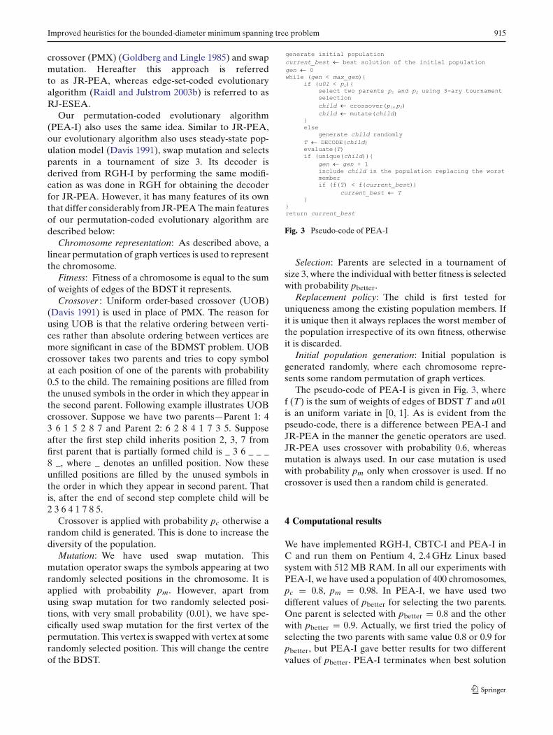
Fig. 3 Pseudo-code of PEA-I

Selection: Parents are selected in a tournament ofsize 3, where the individual with better fitness is selectedwith probability pbetter.

Replacement policy: The child is first tested foruniqueness among the existing population members. Ifit is unique then it always replaces the worst member ofthe population irrespective of its own fitness, otherwiseit is discarded.

Initial population generation: Initial population isgenerated randomly, where each chromosome repre-sents some random permutation of graph vertices.

The pseudo-code of PEA-I is given in Fig. 3, wheref (T) is the sum of weights of edges of BDST T and u01is an uniform variate in [0, 1]. As is evident from thepseudo-code, there is a difference between PEA-I andJR-PEA in the manner the genetic operators are used.JR-PEA uses crossover with probability 0.6, whereasmutation is always used. In our case mutation is usedwith probability pm only when crossover is used. If nocrossover is used then a random child is generated.

4 Computational results

We have implemented RGH-I, CBTC-I and PEA-I inC and run them on Pentium 4, 2.4 GHz Linux basedsystem with 512 MB RAM. In all our experiments withPEA-I, we have used a population of 400 chromosomes,pc = 0.8, pm = 0.98. In PEA-I, we have used twodifferent values of pbetter for selecting the two parents.One parent is selected with pbetter = 0.8 and the otherwith pbetter = 0.9. Actually, we first tried the policy ofselecting the two parents with same value 0.8 or 0.9 forpbetter, but PEA-I gave better results for two differentvalues of pbetter. PEA-I terminates when best solution

916 A. Singh, A. K. Gupta

of the population does not improve over 100,000 newchromosomes. To allow a fair comparison with JR-PEAand RJ-ESEA, we have used the same population sizeand termination condition in PEA-I. Other parame-ters were set to their respective values after a largenumber of trials. Though these parameter valuesprovide good results, they may not be optimal for allinstances. We have tested RGH-I, CBTC-I and PEA-I on the same instances as used in Julstrom and Raidl(2003), Julstrom (2004a,b) and Raidl and Julstrom(2003b). There are two types of instances—Euclideanand non-Euclidean. Only Euclidean instances are usedin Julstrom and Raidl (2003), Julstrom (2004a), Raidland Julstrom (2003b), whereas in Julstrom (2004b) bothtypes of instances are used.

4.1 Results on Euclidean instances

There are in all 30 Euclidean instances with fiveinstances for each value of n = 50, 70, 100, 250, 500 and1,000 vertices. Originally, these instances were designedfor the Euclidean Steiner Tree problem. These instancesare available from Beasley’s OR-library (http://www.people.brunel.ac.uk/∼mastjjb/jeb/info.html). Actually,

there are 15 instances of each size and first five instancesof each size are used for the BDMST problem. Theseinstances consist of points in the unit square. Thesepoints can be considered as the vertices of a completegraph whose weights are the Euclidean distancesbetween them. The diameter bound k is set to 5, 7, 10, 15,20 and 25 for problems of size n = 50, 70, 100, 250, 500and 1,000, respectively.

Table 1 compares the performance of RGH-I andCBTC-I with OTTC, RGH and CBTC on Euclideaninstances. Data for OTTC and RGH are taken fromRaidl and Julstrom (2003b), where the results arereported only on 25 instances excepting the instances ofsize 70. Data for CBTC is taken from Julstrom (2004b),where the results on only 20 instances are reported,excepting the instances of size 50 and 70. However,we have executed CBTC on instances of size 50 also.OTTC, CBTC and CBTC-I were executed n times oneach instance starting from each vertex in turn. BothRGH and RGH-I were executed n times, each timewith a random start vertex. For each instance Table 1reports the best and the average solution found by eachalgorithm as well as the standard deviation of solutionvalues. For CBTC, standard deviations of solution val-ues are not reported in Julstrom (2004b). On Euclid-

Table 1 Results of OTTC, RGH, RGH-I, CBTC and CBTC-I on 25 Euclidean instances of BDMST problem of size 50, 100, 250, 500and 1,000

Instance OTTC RGH RGH-I CBTC CBTC-I

n k Number Best Avg. SD Best Avg. SD Best Avg. SD Best Avg. Best Avg. SD

50 5 1 13.84 21.18 4.82 9.34 12.82 2.48 8.53 12.57 2.13 13.84 21.86 13.28 21.80 5.3350 5 2 14.20 18.15 2.75 8.98 11.56 1.56 8.74 11.39 1.48 13.32 19.29 13.19 19.23 3.7350 5 3 12.53 18.06 2.79 8.76 11.54 1.90 8.28 10.66 1.21 11.62 19.10 11.59 19.06 3.8250 5 4 11.04 15.81 2.78 7.47 10.57 1.66 7.54 9.83 1.51 11.04 16.86 10.78 16.79 3.6550 5 5 13.04 17.77 2.32 8.79 10.91 1.61 8.59 10.52 1.48 12.31 18.36 12.31 18.30 3.28

100 10 1 18.79 29.01 6.53 9.35 10.77 0.81 9.16 10.21 0.75 17.50 28.80 17.35 28.66 7.06100 10 2 17.69 25.24 4.54 9.41 10.80 0.81 9.09 10.45 1.00 15.02 26.95 14.17 26.77 6.24100 10 3 20.16 24.25 4.35 9.75 11.25 0.90 9.39 10.73 0.70 18.37 29.66 17.70 29.48 7.71100 10 4 17.64 26.40 6.27 9.55 11.03 0.89 9.14 10.57 0.88 15.11 28.77 14.92 28.65 7.87100 10 5 16.63 28.63 5.65 9.78 11.36 1.06 9.61 10.95 0.87 15.73 29.46 14.78 29.30 7.83250 15 1 42.09 68.50 14.54 15.14 16.51 0.69 14.61 15.89 0.45 41.61 72.35 39.70 72.07 19.92250 15 2 52.38 71.21 10.67 15.20 16.33 0.67 14.82 15.73 0.42 32.43 75.52 31.59 75.35 19.49250 15 3 43.40 65.38 13.63 15.08 16.19 0.56 14.75 15.68 0.44 32.65 70.60 32.01 70.32 18.22250 15 4 46.76 72.45 10.52 15.49 16.77 0.62 15.14 16.15 0.43 32.29 76.23 31.78 76.09 20.15250 15 5 39.54 64.63 13.68 15.42 16.53 0.58 14.99 15.91 0.45 35.90 71.56 35.79 71.40 17.97500 20 1 90.67 147.69 33.85 21.72 22.86 0.51 21.10 22.07 0.39 80.76 150.68 72.07 150.46 41.40500 20 2 85.34 141.09 29.96 21.46 22.52 0.46 20.81 21.78 0.38 70.44 148.75 70.17 148.54 39.96500 20 3 69.37 148.40 32.66 21.51 22.78 0.50 20.89 22.03 0.37 69.37 153.17 68.83 152.96 39.11500 20 4 89.34 144.11 30.81 21.82 22.85 0.47 21.15 22.10 0.39 63.88 150.98 63.17 150.79 39.24500 20 5 85.35 145.69 38.78 21.37 22.52 0.51 20.84 21.75 0.39 72.36 150.68 72.07 150.46 41.40

1,000 25 1 184.49 320.80 74.86 30.97 32.19 0.41 29.93 31.17 0.40 173.23 327.50 172.62 327.30 83.021,000 25 2 189.50 321.37 69.94 30.90 32.05 0.42 29.85 31.04 0.39 173.85 323.72 173.06 323.50 81.411,000 25 3 184.24 294.56 68.95 30.69 31.77 0.42 29.36 30.77 0.38 175.80 321.25 175.47 321.04 83.101,000 25 4 192.30 312.01 73.06 30.93 32.18 0.43 29.99 31.13 0.38 163.89 323.45 163.43 323.23 80.221,000 25 5 193.02 310.08 56.18 30.85 31.93 0.42 29.81 30.89 0.39 149.36 325.96 148.37 325.76 78.41

Improved heuristics for the bounded-diameter minimum spanning tree problem 917

ean instances, Table 1 clearly shows the superiority ofRGH-I over RGH, OTTC, CBTC and CBTC-I. Thebest as well as average solutions found by the RGH-Iare always better than that of RGH, OTTC, CBTC andCBTC-I except for one instance of size 50, where bestsolution found by RGH is better than that of RGH-I.Standard deviations of solution values are also small forRGH-I. CBTC-I also performs better than CBTC.

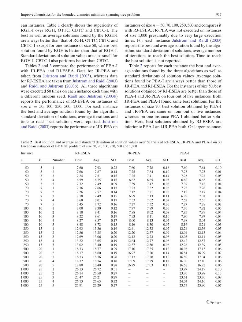
Tables 2 and 3 compare the performance of PEA-Iwith JR-PEA and RJ-ESEA. Data for JR-PEA aretaken from Julstrom and Raidl (2003), whereas datafor RJ-ESEA are taken from Julstrom and Raidl (2003)and Raidl and Julstrom (2003b). All three algorithmswere executed 50 times on each instance each time witha different random seed. Raidl and Julstrom (2003b)reports the performance of RJ-ESEA on instances ofsize n = 50, 100, 250, 500, 1,000. For each instancethe best and average solution found by the algorithm,standard deviation of solutions, average iterations andtime to reach best solutions were reported. Julstromand Raidl (2003) reports the performance of JR-PEA on

instances of size n = 50, 70, 100, 250, 500 and compares itwith RJ-ESEA. JR-PEA was not executed on instancesof size 1,000 presumably due to very large executiontimes. For each instance Julstrom and Raidl (2003)reports the best and average solution found by the algo-rithm, standard deviation of solutions, average numberof iterations to reach the best solution. Time to reachthe best solution is not reported.

Table 2 reports for each instance the best and aver-age solutions found by the three algorithms as well asstandard deviations of solution values. Average solu-tions found by PEA-I are always better than those ofJR-PEA and RJ-ESEA. For the instances of size 50, bestsolutions obtained by RJ-ESEA are better than those ofPEA-I and JR-PEA on four out of five instances. BothJR-PEA and PEA-I found same best solutions. For theinstances of size 70, best solution obtained by PEA-Iand JR-PEA are same on four out of five instances,whereas on one instance PEA-I obtained better solu-tion. Here, best solutions obtained by RJ-ESEA areinferior to PEA-I and JR-PEA both. On larger instances

Table 2 Best solution and average and standard deviation of solution values over 50 trials of RJ-ESEA, JR-PEA and PEA-I on 30Euclidean instances of BDMST problem of size 50, 70, 100, 250, 500 and 1,000

Instance RJ-ESEA JR-PEA PEA-I

n k Number Best Avg. SD Best Avg. SD Best Avg. SD

50 5 1 7.60 7.93 0.22 7.60 7.78 0.16 7.60 7.64 0.1050 5 2 7.68 7.87 0.14 7.75 7.84 0.10 7.75 7.75 0.0150 5 3 7.24 7.51 0.15 7.25 7.41 0.14 7.25 7.27 0.0550 5 4 6.59 6.75 0.15 6.62 6.65 0.05 6.62 6.63 0.0250 5 5 7.32 7.49 0.09 7.39 7.47 0.08 7.39 7.42 0.0470 7 1 7.36 7.66 0.13 7.23 7.32 0.06 7.23 7.28 0.0470 7 2 7.26 7.57 0.14 7.12 7.21 0.06 7.12 7.17 0.0470 7 3 7.18 7.49 0.15 6.99 7.13 0.11 6.99 7.01 0.0370 7 4 7.68 8.01 0.17 7.53 7.62 0.07 7.52 7.55 0.0370 7 5 7.45 7.72 0.16 7.27 7.32 0.06 7.27 7.28 0.02

100 10 1 8.00 8.30 0.12 7.77 7.89 0.06 7.76 7.82 0.03100 10 2 8.10 8.41 0.16 7.88 8.02 0.08 7.85 7.89 0.04100 10 3 8.22 8.61 0.19 7.93 8.11 0.10 7.90 7.97 0.04100 10 4 8.27 8.57 0.17 8.00 8.13 0.07 7.98 8.04 0.03100 10 5 8.48 8.72 0.15 8.16 8.30 0.07 8.16 8.21 0.03250 15 1 12.93 13.36 0.19 12.41 12.52 0.07 12.24 12.36 0.05250 15 2 12.86 13.25 0.20 12.20 12.37 0.09 12.04 12.13 0.04250 15 3 12.69 13.06 0.20 12.12 12.23 0.08 12.03 12.11 0.05250 15 4 13.22 13.65 0.19 12.64 12.77 0.08 12.42 12.57 0.05250 15 5 13.02 13.40 0.19 12.37 12.56 0.08 12.28 12.39 0.05500 20 1 18.33 18.77 0.29 17.10 17.35 0.12 16.96 17.13 0.06500 20 2 18.17 18.60 0.19 16.97 17.20 0.14 16.81 16.99 0.07500 20 3 18.33 18.76 0.28 17.13 17.28 0.10 16.89 17.04 0.06500 20 4 18.32 18.74 0.18 17.09 17.29 0.12 16.96 17.10 0.06500 20 5 17.80 18.40 0.28 16.79 17.03 0.15 16.58 16.72 0.06

1,000 25 1 26.13 26.72 0.31 − − – 23.97 24.19 0.101,000 25 2 26.14 26.58 0.27 − − – 23.70 23.98 0.131,000 25 3 25.47 26.21 0.29 − − – 23.61 23.76 0.081,000 25 4 26.13 26.65 0.22 − − – 24.04 24.16 0.071,000 25 5 25.91 26.29 0.27 − − – 23.75 23.90 0.07

918 A. Singh, A. K. Gupta

Table 3 Average time and average number of iterations required by RJ-ESEA, JR-PEA and PEA-I to reach the best solution on 30Euclidean instances of BDMST problem of size 50, 70, 100, 250, 500 and 1,000

Instance RJ-ESEA JR-PEA PEA-I

n k Number Iterations Time (s)a Iterations Iterations Time (s)

50 5 1 33,947 8.6 36,926 23,448 0.3950 5 2 36,403 9.2 27,955 10,004 0.1750 5 3 27,919 7.1 31,725 24,443 0.4150 5 4 31,382 7.9 40,703 11,825 0.2050 5 5 34,924 8.9 34,369 24,927 0.4270 7 1 82,351 − 68,863 61,246 1.2970 7 2 65,581 − 61,106 47,255 1.0170 7 3 79,838 − 64,824 47,132 0.9970 7 4 56,401 − 54,316 41,869 0.8970 7 5 83,404 − 71,344 41,684 0.89

100 10 1 189,026 105.0 88,831 103,262 2.88100 10 2 205,891 114.6 82,560 83,394 2.31100 10 3 176,043 97.0 88,467 136,975 3.74100 10 4 163,142 90.3 92,993 113,883 3.16100 10 5 164,651 90.5 89,735 114,407 3.22250 15 1 471,803 809.0 278,984 386,197 26.35250 15 2 466,047 796.7 311,349 367,366 25.18250 15 3 464,618 796.8 309,699 406,414 26.66250 15 4 442,446 758.3 305,125 425,633 28.44250 15 5 497,450 856.9 316,006 351,804 23.52500 20 1 527,659 2, 140.0 712,011 818,202 124.63500 20 2 652,009 2, 672.2 736,921 833,715 134.12500 20 3 504,315 2, 050.6 746,259 892,252 137.94500 20 4 654,871 2, 658.5 742,231 872,195 155.62500 20 5 648,148 2, 673.7 705,313 848,124 130.08

1,000 25 1 501,047 4, 535.3 − 1,768,532 1,148.721,000 25 2 464,397 4, 191.6 − 1,527,331 990.631,000 25 3 554,601 5, 018.4 − 1,783,477 1,120.101,000 25 4 508,038 4, 589.1 − 1,730,925 1,124.681,000 25 5 647,818 5, 911.8 − 1,681,034 1,086.25

aExecution time on Pentium III, 800 MHz

best solutions obtained by PEA-I are always superior toJR-PEA and RJ-ESEA.

Table 3 reports the average number of iterationsrequired by the three algorithms to reach the best solu-tion. It also reports the average time taken by RJ-ESEAand PEA-I to reach the best solutions. Average times ofRJ-ESEA on instances of size 70 are not reported inthe table as data for instances of size 70 are taken fromJulstrom and Raidl (2003) where execution times arenot reported. Though on large instances PEA-I requiremore iteration to reach the best solutions, it obtainssolutions of better quality. This can be attributed to pre-mature convergence of RJ-ESEA and JR-PEA.

RJ-ESEA and JR-PEA were executed on PentiumIII, 800 MHz system. As RJ-ESEA and PEA-I were exe-cuted on different systems it is not possible to exactlycompare the speed of two algorithms, but even afterassuming that our system is four times faster thanPentium III 800 MHz, PEA-I is faster than RJ-ESEA.Moreover, since PEA-I takes more iterations to find

the solution, time per iteration of PEA-I is even muchsmaller than RJ-ESEA. This is significant as the worstcase time complexity of each iteration of PEA-I is O(n2),whereas that of RJ-ESEA is O(n). This became possi-ble due to the use of sorted cost matrix. To get an ideaof the speed-up of PEA-I due to the use of sorted costmatrix we have also implemented PEA-I without thesorted cost matrix and executed it on one instance ofeach size n = 50, 70, 100, 250, 500 vertices. On instanceof size 1,000 we are not able to execute PEA-I with-out sorted cost matrix due to very large execution time.Table 4 compares the average time required by the twoversions of PEA-I. PEA-I with sorted cost matrix isalways faster than PEA-I without it and the differencein speed grows with n. On instance of size 500, PEA-Iwith sorted cost matrix is more than 50 times faster thanPEA-I without it.

Table 5 compares the performance of two gener-ational evolutionary algorithms proposed in Julstrom(2004a) with PEA-I. In Table 5, the permutation-coded

Improved heuristics for the bounded-diameter minimum spanning tree problem 919

Table 4 Comparison of average time taken to reach the best solution by PEA-I with sorted cost matrix and PEA-I without it

Instance PEA-I with sorted cost matrix PEA-I without sorted cost matrix

n k Number Avg. time (s) Avg. time (s)

50 5 1 0.39 0.5670 7 1 1.29 3.03100 10 1 2.88 11.63250 15 1 26.35 425.82500 20 1 124.63 6, 671.21

Table 5 Best solution and average and standard deviation of solution values over 50 trials of J-GPEA, J-GRKEA and PEA-I on 25Euclidean instances of BDMST problem of size 50, 70, 100, 250, 500

Instance J-GPEA J-GRKEA PEA-I

n k Number Best Avg. SD Best Avg. SD Best Avg. SD

50 5 1 7.60 7.84 0.19 7.61 7.85 0.13 7.60 7.64 0.1050 5 2 7.75 7.89 0.12 7.75 7.87 0.10 7.75 7.75 0.0150 5 3 7.25 7.48 0.15 7.25 7.49 0.14 7.25 7.27 0.0550 5 4 6.62 6.68 0.09 6.62 6.71 0.10 6.62 6.63 0.0250 5 5 7.39 7.50 0.12 7.39 7.49 0.07 7.39 7.42 0.0470 7 1 7.24 7.36 0.07 7.23 7.36 0.06 7.23 7.28 0.0470 7 2 7.12 7.23 0.08 7.12 7.25 0.07 7.12 7.17 0.0470 7 3 6.99 7.20 0.14 7.01 7.15 0.10 6.99 7.01 0.0370 7 4 7.52 7.65 0.10 7.52 7.64 0.07 7.52 7.55 0.0370 7 5 7.27 7.36 0.08 7.27 7.34 0.05 7.27 7.28 0.02

100 10 1 7.82 7.92 0.07 7.83 7.92 0.05 7.76 7.82 0.03100 10 2 7.87 8.02 0.08 7.85 8.04 0.09 7.85 7.89 0.04100 10 3 7.99 8.14 0.08 7.98 8.14 0.09 7.90 7.97 0.04100 10 4 8.01 8.14 0.07 8.00 8.12 0.06 7.98 8.04 0.03100 10 5 8.19 8.34 0.08 8.20 8.31 0.08 8.16 8.21 0.03250 15 1 12.44 12.60 0.08 12.45 12.58 0.08 12.24 12.36 0.05250 15 2 12.24 12.43 0.10 12.22 12.39 0.10 12.04 12.13 0.04250 15 3 12.12 12.28 0.08 12.18 12.32 0.07 12.03 12.11 0.05250 15 4 12.57 12.82 0.11 12.63 12.80 0.07 12.42 12.57 0.05250 15 5 12.36 12.61 0.12 12.38 12.62 0.10 12.28 12.39 0.05500 20 1 17.22 17.48 0.10 17.16 17.43 0.10 16.96 17.13 0.06500 20 2 17.09 17.31 0.11 17.10 17.29 0.10 16.81 16.99 0.07500 20 3 17.17 17.45 0.11 17.16 17.37 0.11 16.89 17.04 0.06500 20 4 17.22 17.48 0.13 17.27 17.43 0.09 16.96 17.10 0.06500 20 5 16.94 17.14 0.11 16.87 17.09 0.11 16.58 16.72 0.06

generational evolutionary algorithm is referred to asJ-GPEA, whereas the random-key-coded generationalevolutionary algorithm is referred to as J-GRKEA. Asshown by the table, PEA-I outperforms J-GPEA andJ-GRKEA both. Data for J-GPEA and J-GRKEA aretaken from Julstrom (2004a), where time to reach thebest solution is not reported. Both J-GPEA andJ-GRKEA were not executed on instances of size 1,000.

4.2 Results on non-Euclidean instances

There are 20 non-Euclidean instances with five instancesfor each value of n = 100, 250, 500 and 1,000 vertices.All of these instances are complete graphs with weightsrandomly chosen from [0.01, 0.99]. The diameter bound

k is set to 10, 15, 20 and 25 for problems of size n = 100,250, 500 and 1,000, respectively. These instances werefirst used in Julstrom (2004b).

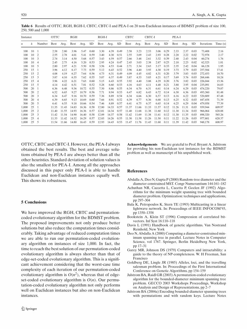
Table 6 compares the performance of RGH-I,CBTC-I and PEA-I with OTTC, RGH and CBTC onnon-Euclidean instances. Data for OTTC, RGH andCBTC are taken from Julstrom (2004b), where stan-dard deviations of solution values for OTTC and CBTCare not reported. As in the case of Euclidean instances,here also PEA-I is executed 50 times on each instance,whereas other heuristics are executed n times on eachinstance. Here also RGH-I and CBTC-I give betterresults than RGH and CBTC, respectively. Here, bothRGH and RGH-I performs much worse than OTTC,CBTC and CBTC-I. Even RGH-I cannot compete with

920 A. Singh, A. K. Gupta

Table 6 Results of OTTC, RGH, RGH-I, CBTC, CBTC-I and PEA-I on 20 non-Euclidean instances of BDMST problem of size 100,250, 500 and 1,000

Instance OTTC RGH RGH-I CBTC CBTC-I PEA-I

n k Number Best Avg. Best Avg. SD Best Avg. SD Best Avg. Best Avg. SD Best Avg. SD Iterations Time (s)

100 10 1 2.58 2.80 3.96 5.47 0.60 3.30 4.39 0.49 2.58 3.23 2.53 3.06 0.29 2.33 2.37 0.03 73,408 2.16100 10 2 2.55 2.78 4.01 5.41 0.59 3.40 4.30 0.51 2.55 3.09 2.43 2.93 0.28 2.20 2.22 0.02 72,978 2.17100 10 3 2.74 3.14 4.50 5.68 0.57 3.43 4.59 0.57 2.66 3.48 2.61 3.32 0.39 2.40 2.43 0.04 60,274 1.76100 10 4 2.45 2.75 4.16 5.20 0.53 2.95 4.24 0.47 2.45 3.03 2.38 2.87 0.25 2.18 2.23 0.02 62,525 1.81100 10 5 2.80 2.97 4.21 5.50 0.58 3.56 4.53 0.44 2.71 3.34 2.63 3.17 0.33 2.35 2.42 0.04 66,128 1.95250 15 1 3.96 4.12 6.17 7.73 0.59 5.12 6.43 0.52 3.96 4.40 3.93 4.30 0.19 3.73 3.79 0.03 257,584 17.41250 15 2 4.08 4.19 6.27 7.64 0.56 4.73 6.31 0.49 4.09 4.45 4.02 4.31 0.20 3.79 3.83 0.03 272,453 18.70250 15 3 3.87 4.10 6.35 7.62 0.55 5.07 6.37 0.49 3.87 4.33 3.83 4.21 0.17 3.69 3.76 0.03 268,446 18.24250 15 4 3.96 4.22 6.21 7.63 0.60 5.15 6.43 0.55 3.92 4.40 3.88 4.29 0.20 3.76 3.82 0.03 226,044 15.36250 15 5 4.14 4.42 6.51 7.81 0.52 5.28 6.60 0.53 4.16 4.63 4.11 4.48 0.21 3.88 3.95 0.04 235,091 16.03500 20 1 6.36 6.48 9.36 10.72 0.55 7.50 8.86 0.55 6.34 6.70 6.31 6.61 0.14 6.24 6.29 0.03 474,220 79.87500 20 2 6.52 6.65 9.27 10.79 0.56 7.71 8.94 0.53 6.47 6.82 6.43 6.72 0.14 6.30 6.36 0.03 493,360 81.48500 20 3 6.34 6.47 9.16 10.70 0.59 7.36 8.89 0.54 6.34 6.66 6.30 6.57 0.13 6.16 6.22 0.03 520,809 87.48500 20 4 6.39 6.65 9.13 10.69 0.60 7.66 8.91 0.52 6.39 6.77 6.36 6.68 0.13 6.25 6.32 0.03 447,458 71.39500 20 5 6.41 6.55 9.18 10.66 0.54 7.46 8.89 0.57 6.41 6.75 6.37 6.65 0.14 6.25 6.29 0.04 479,958 77.39

1,000 25 1 11.35 11.43 14.83 16.36 0.58 12.80 14.33 0.57 11.37 11.66 11.33 11.57 0.12 11.26 11.31 0.03 939,944 609.971,000 25 2 11.40 11.55 14.93 16.36 0.57 12.81 14.34 0.57 11.40 11.68 11.38 11.60 0.12 11.30 11.34 0.03 966,064 620.881,000 25 3 11.42 11.54 14.90 16.40 0.58 12.89 14.37 0.58 11.42 11.69 11.38 11.61 0.12 11.30 11.35 0.03 898,320 585.261,000 25 4 11.33 11.42 14.52 16.29 0.57 12.83 14.26 0.55 11.30 11.58 11.26 11.50 0.11 11.22 11.26 0.03 977,801 628.371,000 25 5 11.54 11.66 14.80 16.43 0.59 12.93 14.43 0.53 11.47 11.76 11.43 11.68 0.11 11.39 11.42 0.03 948,178 608.97

OTTC, CBTC and CBTC-I. However, the PEA-I alwaysobtained the best results. The best and average solu-tions obtained by PEA-I are always better than all theother heuristics. Standard deviation of solution values isalso the smallest for PEA-I. Among all the approachesdiscussed in this paper only PEA-I is able to handleEuclidean and non-Euclidean instances equally well.This shows its robustness.

5 Conclusions

We have improved the RGH, CBTC and permutation-coded evolutionary algorithm for the BDMST problem.The proposed improvements not only produce bettersolutions but also reduce the computation times consid-erably. Taking advantage of reduced computation timeswe are able to run our permutation-coded evolution-ary algorithm on instances of size 1,000. In fact, thetime to reach the best solution of our permutation-codedevolutionary algorithm is always shorter than that ofedge-set-coded evolutionary algorithm. This is a signifi-cant achievement considering that the worst-case timecomplexity of each iteration of our permutation-codedevolutionary algorithm is O(n2), whereas that of edge-set-coded evolutionary algorithm is O(n). Our permu-tation-coded evolutionary algorithm not only performswell on Euclidean instances but also on non-Euclideaninstances.

Acknowledgements We are grateful to Prof. Bryant A. Julstromfor providing his non-Euclidean test instances for the BDMSTproblem as well as manuscript of his unpublished work.

References

Abdalla A, Deo N, Gupta P (2000) Random-tree diameter and thediameter constrained MST. Congr Numerantium 144:161–182

Achuthan NR, Caccetta L, Cacetta P, Geelen JF (1992) Algo-rithms for the minimum weight spanning tree with boundeddiameter problem. Optimization: techniques and applications,pp 297–304

Bala K, Petropoulos K, Stern TE (1993) Multicasting in a linearlightwave network. In: Proceedings of IEEE INFOCOM’93,pp 1350–1358

Bookstein A, Klein ST (1996) Compression of correlated bit-vectors. Inf Syst 16:110–118

Davis L (1991) Handbook of genetic algorithms. Van NostrandReinhold, New York

Deo N, Abdalla A (2000) Computing a diameter-constrained min-imum spanning tree in parallel. Lecture Notes in ComputerScience, vol 1767. Springer, Berlin Heidelberg New York,pp 17–31

Garey MR, Johnson DS (1979) Computers and intractability: aguide to the theory of NP-completeness. W. H Freeman, SanFrancisco

Goldberg DE, Lingle JR (1985) Alleles, loci, and the travellingsalesman problem. In: Proceedings of the First InternationalConference on Genetic Algorithms, pp 154–159

Julstrom BA, Raidl GR (2003) A permutation-coded evolutionaryalgorithm for the bounded-diameter minimum spanning treeproblem. GECCO 2003 Workshops Proceedings, Workshopon Analysis and Design of Representations, pp 2–7

Julstrom BA (2004a) Encoding bounded-diameter spanning treeswith permutations and with random keys. Lecture Notes

Improved heuristics for the bounded-diameter minimum spanning tree problem 921

in Computer Science, vol 3102. Springer, Berlin HeidelbergNew York, pp 1272–1281

Julstrom BA (2004b) Greedy heuristics for the bounded-diameterminimum spanning tree problem. Communicated to ACM JExp Algorithmics

Kortsarz G, Peleg D (1997) Approximating shallow-light trees. In:Proceedings of the 8th Symposium on Discrete Algorithms,pp 103–110

Kortsarz G, Peleg D (1999) Approximating the weight of shallowSteiner trees. Discrete Appl Math 93:265–285

Prim R (1957) Shortest connection networks and some general-izations. Bell Syst Tech J 36:1389–1401

Raidl GR, Julstrom BA (2003a) Edge-sets: an effective evolu-tionary coding of spanning trees. IEEE Trans Evol Comput7:225–239

Raidl GR, Julstrom BA (2003b) Greedy heuristics and anevolutionary algorithm for the bounded-diameter minimum

spanning tree problem. In: Proceedings of the 2003 ACMSymposium on Applied Computing, pp 747–752

Raymond K (1989) A tree-based algorithm for distributed mutualexclusion. ACM Trans Comput Syst 7:61–77

Reeves CR (1995) A genetic algorithm for flowshop sequencing.Comput Oper Res 22:5–13

Satyanarayanan R, Muthukrishnan DR (1992) A note onRaymond’s tree-based algorithm for distributed mutual exclu-sion. Inf Process Letters 43:249–255

Satyanarayanan R, Muthukrishnan DR (1994) A static tree-basedalgorithm for the distributed readers and writers problem.Comput Sci Inform 24:21–32

Wang S, Lang SD (1994) A tree-based distributed algorithm forthe k-entry critical section problem. In: Proceedings of the1994 International Conference on Parallel and DistributedSystems, pp 592–597