Implicit Surface Visualization of

Reconstructed Biological Molecules

Edgar Garduno and Gabor T. Herman

presented by Adriana Wise

Thursday, March 18th, 2004

Contents

*List of Slides

1 Contents

2 Introduction

6 Blob Representation/Implicit Surfaces

7 Reconstruction

9 Blobs and Grids

11 Basic Raycasting-Blobs Technique for Visualization

13 Main Blob Raycasting Algorithm

14 First Experiment Set. Visualization of Reconstructed

Molecules through Plain Blob Raycasting Algorithm

15 Improved Method to Speed Up the Blob Raycasting

Technique

16 Second Experiment Set. Visualization of Reconstructed

Molecules through Improved Blob Raycasting Algorithm

17 Conclusion

Introduction

The transmission electron microscope (TEM) captures projec-

tions from different directions of a molecule, as two-dimensional

density functions. These are processed via a reconstruction al-

gorithm, which outputs a three-dimensional electron density dis-

tribution.

(TEMs work the same way as slide projectors, except that they

shine (transmit) a beam of electrons (instead of light) through

the specimen (instead of the slide). Whatever part is transmitted

is projected onto a phosphor screen for the user to see.)

The three-dimensional density distribution is represented as a lin-

ear combination of basis functions, or blobs, chosen a priori to

have certain desired particularities, such as smoothness (differ-

entiable in all points) and zero values outside a bounded support

(their Fourier Transform are close-to-zero sufficiently far away

from the origin).

The reconstruction algorithm departs from a set of chosen such

functions and calculates the coefficients in the linear combina-

tion:

ν(x) =J∑

j=1

(cj · bj(x)) (1)

where:

x – a point in the three-dimensional space, x ∈ R3;

ν(x) – three-dimensional density function, output by ART;

J – the number of basis functions;

bj(x) – the jth basis function (blob).

The scope of this paper is to visualize the three-dimensional sur-

face describing the density function resulted from reconstruction,

through a procedure that departs directly from over a million ba-

sis functions (blobs) and produces two-dimensional projections

on the visual screen of implicit 3-D surfaces of equal density.

In contrast, the existing methods produced projections on the

visual screen based on an intermediate stage of polygonalization,

which can introduce substantial inaccuracies, both in the position

of the 3-D surface being visualized, and in the angle of normals

to that surface at various points.

The main idea behind using directly the blob-based representa-

tion of the density function for visualization as a 2-D projection is

taking “depth cues to deliver the three-dimensional information

contained in the density functions” (p.3). The method used,

namely raycasting, calculates the angles between a multitude of

rays being cast from the visual screen and the normals to the

isosurface at the points of intersection. Isosurfaces are sets of

points where the density function has a particular value. It also

uses, to a lesser extent, the lengths of these rays (i.e. distance

between screen and intersection point). This information is as-

sociated with corresponding intensities of color on the display

screen, that create the image of the 3-D object being investi-

gated.

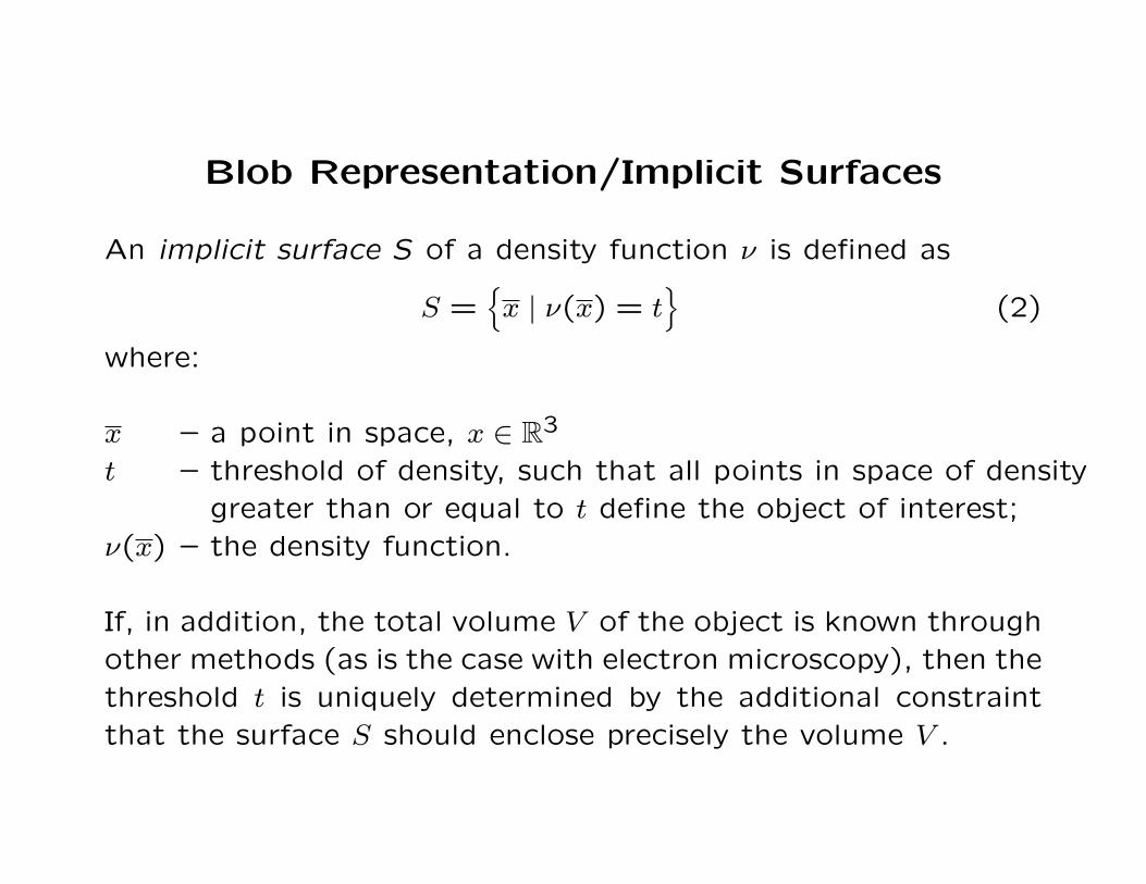
Blob Representation/Implicit Surfaces

An implicit surface S of a density function ν is defined as

S ={x | ν(x) = t

}(2)

where:

x – a point in space, x ∈ R3

t – threshold of density, such that all points in space of densitygreater than or equal to t define the object of interest;

ν(x) – the density function.

If, in addition, the total volume V of the object is known throughother methods (as is the case with electron microscopy), then thethreshold t is uniquely determined by the additional constraintthat the surface S should enclose precisely the volume V .

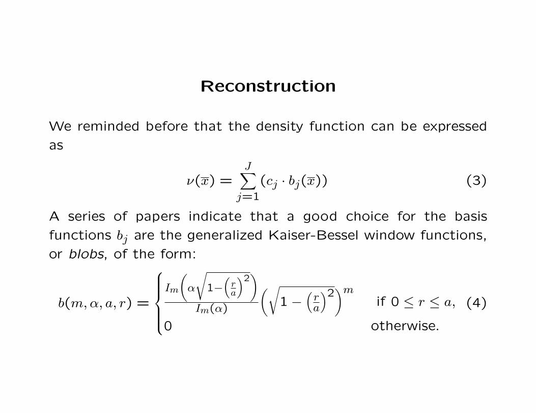
Reconstruction

We reminded before that the density function can be expressed

as

ν(x) =J∑

j=1

(cj · bj(x)) (3)

A series of papers indicate that a good choice for the basis

functions bj are the generalized Kaiser-Bessel window functions,

or blobs, of the form:

b(m, α, a, r) =

Im

(α

√1−

(ra

)2)

Im(α)

(√1−

(ra

)2)m

if 0 ≤ r ≤ a,

0 otherwise.

(4)

where:

r – distance from blob center of a point x ∈ R3

whose local density is returned by corresponding bj(m, α, a, r)

(all points of equal r in blob bj have equal density);

a – the radius of the sphere that is the support of the blob;

α – blob shape parameter;

Im – modified Bessel function of order m:

Im(x) = (−i)m · Jm(ix)

Jm(x) =∞∑

n=0

(−1)n · x2n+m

n!(n + m)!22n+m

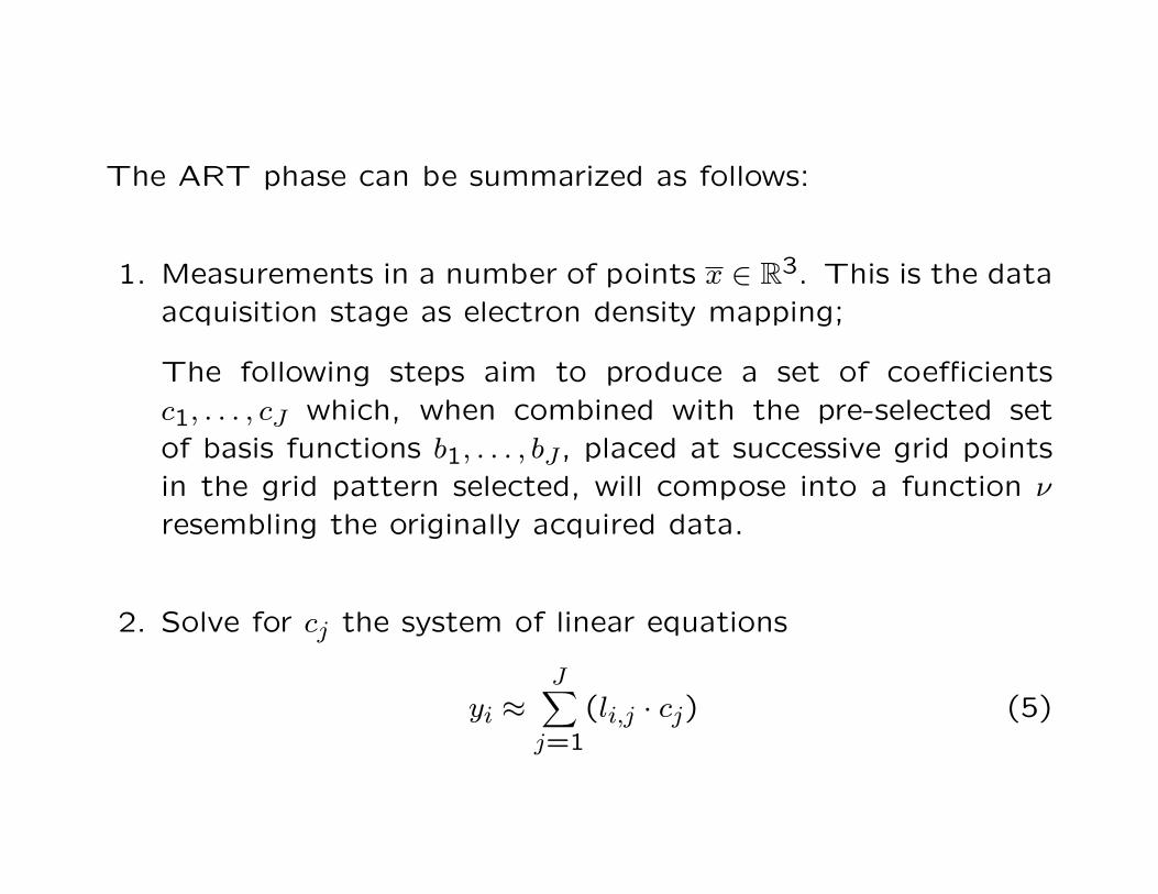
The ART phase can be summarized as follows:

1. Measurements in a number of points x ∈ R3. This is the dataacquisition stage as electron density mapping;

The following steps aim to produce a set of coefficientsc1, . . . , cJ which, when combined with the pre-selected setof basis functions b1, . . . , bJ, placed at successive grid pointsin the grid pattern selected, will compose into a function ν

resembling the originally acquired data.

2. Solve for cj the system of linear equations

yi ≈J∑

j=1

(li,j · cj) (5)

(or y = L · c), where

li,j = [Pν](−→o , x) (6)

and

[Pν](−→o , x) =∫R

ν(x + τ−→o )dτ (7)

is the ray transform of ν along vector −→o ;

3. Calculate ν(x) in xj ∈ X ⊂ R3 from grid using ν(x) =∑J

j=1 cj ·bj(x);

4. Determine surface St ={x | ν(x) = t

}such that the volume

enclosed by St is the measured volume V .

Blobs and Grids

Considering a body-centered cubic grid (bcc), the choices of the

bj parameters will relate to the bcc ∆ distance and to other

desirable basis functions properties as follows:

a – it has been empirically shown that small a values are OK.

Big blobs will not yield results that preserve concavities

in a known original 3-D object. Blobs with large support

can still be ”skinny” by choosing α appropriately.

The main problem with large support is the computational cost.

m – order of modified Bessel function m = 2;

α – argument of I2. For considerations related to

the convolution of the blob bj with a truncated version of

the train of pulses XB∆, where F{b} should be

zero-valued at the locations of the pulses in F{XB∆}

closest to origin, α should be selected as below:

α =

√2π2

( a

∆

)2− 6.9879322

Basic Raycasting-Blobs Technique for

Visualization

As briefly mentioned in the introduction, the raycasting tech-

nique consists of intersecting rays cast perpendicularly from the

viewing plane onto S, the implicit surface defined by ν(x). The

lengths of such rays hitting a portion of the implicit surface

“closest” to the viewing plane are mapped onto different color

intensities to create the illusion of a 3D object in a 2D environ-

ment.

The innovative contribution of this paper is twofold: it applies

raycasting directly to blobs, and not to polygons which appear

as an intermediate step in existing raycasting procedures. This

will significantly reduce the level of inaccuracy, already present at

the stages of data capture and reconstruction. Secondly, it pro-

poses an optimization algorithm for the rendering stage,

which the new blob raycasting technique lends itself to, and

which spectacularly reduces the display time from hours to sec-

onds.

The challenge is, then, finding points q ∈ R3 of intersection of

rays R with the implicit surface S, such that the distance between

q and the viewing screen is minimal:

minq=R

⋂S

{dist(q, screen)

}(8)

There are procedures published in the literature that guarantee

finding such intersections, where they exist. These procedures

are dependent on ν(x)’s derivatives, which are easy to compute

analytically from the formula of ν(x) =∑J

j=0 cj · bj(x), and, in

turn, bj(x) can be also analytically differentiated from the formula

of bj(m, α, a, r). However, in these procedures, the step size for

the search is inversely proportional to the large number of basis

functions contributing to the value of ν in a given point, which

makes them computationally unacceptable.

The alternative, presented in this paper, consists of preprocessing

the set of grid centers{pj

}such that, for every distinct R, all

possible intersections q = R⋂

S of R with the isosurface S are

ordered by the distance dist(q, screen). Then all but the smallest

such distances are eliminated (intuitively, thus ensuring that only

the surface that should contribute to the projection on the visual

screen is retained).

This minimal distance minR⋂

S

{dist(qt, screen)

}is determined

as the intersection point qt, nearest to the screen, encountered

along the projection ray R, that satisfies ν(q) = t (i.e. that is on

the isosurface determined by the density threshold t):

dR = minq∈R3

{dq | ν(q) = t

}(9)

In other words, instead of a set of intersections of purely geo-

metric entities (as is the case with raytracing techniques applied

to surfaces approximated through polygonalization), this paper

proposes a set of points at the intersection of rays R with im-

plicit surfaces. Further optimizations can be made to reduce

the computational complexity, by reducing the number of grid

centers whose blobs might influence the density function at the

intersection with the projection ray.

We will try to present in what follows a sketch of the algorithmic

steps considered in the new blob raytracing method.

Main Blob Raycasting Algorithm

Prior to applying the algorithm, which iterates after the number

of rays cast from the visual screen: create 1-dimensional tables,

one table per blob, mapping radial distance (of various points

inside the blob from the grid center) onto pre-calculated pairs

(bj, cj) of basis functions and appropriate coefficients for each

blob bj. Due to radial symmetry, different points x equidistant

to the grid center of bj will have the same pair (bj, cj) (the value

varying with r being bj).

The composite value of the density function for any point x ∈ R3

can be then simply calculated by the sum of the products bj(x)·cj

that are found in the look-up tables by the key x.

1. For each R, eliminate all blobs of grid centers farther than a

from R, which cannot possibly influence ν(q) along R (elim-

inate blobs with null intersection bj⋂

R = ∅);

2. Find projections of all blobs (still remaining after (1)), cut

by R, in order of closeness to the visual screen;

3. For all remaining grid points whose blobs cut R, now also

conveniently ordered, as per step (2), in decreasing distance

from the screen, evaluate ν at the intersection between R

and the normal of the grid point on R.

ray R

blob b j

grid center p j

blob b j+1

grid center p j+1

projection q j

projection q j+1

loci of points of equal density in b j (spheres)

ray R

blob b j

p j blob b j+1

p j+1

projection q j

projection q j+1

section of simple isosurface from

intersection of b j and b j+1 ; t=6, and is obtained from

local contributions of points of densities (3,3) and (1,5)

1 3 5 9

1 3 5 9

6 6

6

4. When two adjacent projections are found, let those qa and

qb, which satisfy

ν(qa) < t but ν(qb) > t, (10)

then go to next step of finding q ∈[qa; qb

]of exact t;

Note: A point x for a grid with bcc distance ∆ and blobs

of radii a is influenced by at most 51 blobs, if a and ∆ are

chosen of particular values.

5. Assuming that points of projection of adjacent grid centers

on R, qa and qb, have been found such that

ν(qa) < t but ν(qb) > t,

use the Newton-Raphson or/and bisection methods on the

interval[qa; qb

]to find points of density exactly t on R be-

tween qa and qb.

Newton-Raphson Root Finding Method — Quick Re-

minder

The N-R method finds roots of polynomials of degree ≥ 5 or

of transcendentals (e.g. cosx = x), r such that f(r) = 0.

f(x)

Y-A

xis

X-Axis

f(x 1 )

x 1

r

L

x 2

f(x 2 )

x 3

L 1

The method chooses an initial approximation of r, as x1,

randomly (or optimized) along f(x). It builds a tangent L1

to f(x) in x1 and finds x2 as L1’s intersection with the x axis.

Now x2 is closer to r than x1, and will be chosen as the next

approximation for r and so on:

f ′(x1) =f(x)− f(x1)

x− x1equation of L1

To find the x2 as the x-intercept of L1, L1(x2) = 0:

x2 = x1 −f(x1)

f ′(x1). . .

In general,

xn+1 = xn −f(xn)

f ′(xn),

with limn→∞ xn = r, if convergence exists.

In our case, finding qt ∈[qa; qb

]is possible if the fact that

ν(qa) < t ∧ ν(qb) < t indicates a local monotony of ν(q) on[qa; qb

]. This is intuitively the case if qa and qb are sufficiently

close, which is (more or less) guaranteed by the grid structureand by the small value(s) chosen for a.

In particular, if convergence exists, x− ν(x)ν′(x) converges quadrat-

ically.

If N-R fails due to non-convergence, then the bisection method(which, albeit slower, is guaranteed to converge) will be ap-plied.

The Bisection Root Finding Method — Quick Reminder

The bisection method chooses two random points x1 andx2 within f ’s domain, such that f(x1) and f(x2) are on ei-ther side of 0. Then it calculates x3 as the middle of the

interval [x1;x2], and the corresponding f(x3). Then a new

interval is chosen, such that both values in the new pair (ei-

ther(f(x1), f(x3)

), or

(f(x3), f(x2)

)) are on different sides

of 0. The iteration goes on until the interval(f(xm), f(xn)

)becomes very small.

In our case, this method presents the potential for an ad-

ditional optimization: the initial interval does not need to

be chosen as big as the difference along R between the pro-

jections[qa, qb

]. Instead, only that interval where the N-R

method was abandoned before it deconverged can be chosen

as a first approximation.

The guarantee presented by the particular properties of the

basis functions bj that at least one of the two methods will

succeed, lies in the fact that, by choice, ν(x) is continuouslydifferentiable, with gradient:

∇ν(x) =J∑

j=1

cj · ∇bj(x) (11)

(Quick reminder: If f is a function of two variables x and y,then the gradient of f is the vector function ∇f :

Duf = ∇f(x, y) =∂f

∂xi +

∂f

∂yj, (12)

where u = 〈i, j〉 is a vector. So ∇f(x, y) is the rate of changeof f in the direction of vector u = 〈i, j〉).

6. Collect all points q as found at (6) (i.e. that are projectionson R of grid centers and are of equal density t), for all projec-

tion rays R cast from the display screen, and color the projec-

tions on the screen according to the distances dist(q, screen).

The result will be a 2-D projection of all points from the 3-D

original object, of chosen equal density t, colored according

to the distance from the display screen.

First Experiment Set. Visualization of

Reconstructed Molecules through Plain Blob

Raycasting Algorithm

Experiment 1:

IN: – molecule: Escherichia Coli, DnaB and DnaC (which “dock”

during E. Coli DNA replication, and thus are of interest);

– ∆ = 12;

– a = 2.40;

– α = 13.26

OUT: – time reconstruction: 65h 22′ 48′′;

– set of coefficients cj: 1,600,065 distinct values

– time visualization: 1h 28′ 12′′

HW: – processor: Pentium IV, 2GHz

– OS: Linux

– RAM: 1GB

– resolution: 512x512

Note: Although the resolution was chosen significantly lowerthan the performance of current display monitors, it would not

have made sense to choose a higher value due to the quality

of the data from which the reconstructions were obtained (you

acquire a density map, which you then try to approximate with a

function; both the acquisition and the approximation/ART are

prone to inaccuracies). A comparison with a known shape was

not available.

Experiment 2:

IN: – molecule: Bacteria Rhodopsin, for which a protein database

(PDB) description is also available (i.e. the density data

is obtained by knowing a priori the shape of the function);

– intermediate step: the so-called “conical tilt scheme” is

used to convert the PDB data into usable input for ART.

The conical tilt scheme yields data resembling/simulatingdata obtained from the e microscope. It introduces someinaccuracy (some dispersion) of the sharp values from thePDB;

– ∆ = 12 (same as for Experiment 1);

– a = 2.40 (same);

– α = 13.26 (same)

OUT: – time reconstruction: 36h 13′ 36′′;

– set of coefficients cj: 1,482,624 distinct values

– time visualization: 1h 37′ 55′′

HW: – processor: Pentium IV, 2GHz

– OS: Linux

– RAM: 1GB

– resolution: 512x512

Preliminary conclusion: Visualization through blob raycasting,

in the absence of further optimizations, is computationally ex-

pensive due to the ν(q)− t = 0 searches for all rays R. And this

— only for one projection!!!

Improved Method to Speed Up the Blob

Raycasting Technique

Within the algorithm presented, the longest computing time is

spent by the search aimed at finding the pairs of consecutive

(adjacent) projections qa, qb for which the images through ν are

on either side of t (i.e. finding even rough initial approximations

for the N-R/bisection methods).

On the other hand, finding q ∈[qa; qb

]such that ν(q) = t is

standard, and cannot be further optimized.

The proposed optimization method is presented below:

1. Calculates for every grid center pj the local value of ν at

points pj:

vj = ν(pj)

2. Uses the set vj and the subset of grid centers for which vj ≥ t

in a “Z-buffer algorithm” that operates as follows:

for all R

length(R) ←∞for all j (i.e. for all blobs) s.t. vj ≥ t

calculate dj = dist(pj, screen)

for all R s.t. (R⋂

bj 6= ∅)R ← min

{R, dj

}

The Z-buffer algorithm approximates, for each blob j whose

bj(pj) ≥ t, the lengths of all rays that intersect it with the

distance of the grid center pj to the screen. By doing so,

it generates a good initial approximation for one of the ex-

tremities of the interval[qa; qb

](more precisely the positive

one, i.e. the one yielding ν(qa)− t ≥ 0).

The change of ν(x) to a value ≤ t will occur between adjacent

grid points, so the other extremity is likely to be found by

taking the value bj(pj+1) of one of the adjacent blobs.

3. Given the set of grid centers with vj ≥ t and their projec-

tions qc on rays intersecting bj as first approximations for

the N-R/bisection methods, apply the modified raycasting

algorithm, described as follows (the projections on R of pj

grid centers are hereafter denoted qc):

for all R s.t. ∃qc = projection of pj on R

check that ν(qc) ≥ t

if (ν(qc) � t)

do the search for[qa; qb

]around qc, by checking

values for ν of all projections

of grid centers pj on R,

(i.o.w. apply plain blob raycasting() )

else

limit search for[qa; qb

]only to points such that{

q ∈ R3 | dist(q, screen) ≤ dist(qc; screen)}

apply blob raycasting()

This is saying that once initial approximations qc have been found

through the Z-buffer algorithm, the N-R/bisection algorithm(s)

will be applied as per the following cases:around qc if ν(qc) � t,

between qc and the plane otherwise.(13)

Remember that, in the absence of the optimization, all adjacent

projections of grid centers were searched, until a pair was found

such that its density values were on different sides of t.

The savings in computation time occur once we start off with

only those projections whose density values are above t, and then

either apply N-R (which only requires one initial approximation),

or find the other extremity of the initial approximation interval

to apply bisection in the vicinity of the current qc, towards the

plane (where the function ν(qc)− t changes sign). Intuitively, the

density function is guaranteed to decrease to a value below t as

we get farther from qc and towards the plane.

Second Experiment Set. Visualization of

Reconstructed Molecules through Improved

Blob Raycasting Algorithm

Experiment 1:

IN: – molecule: Escherichia Coli;

– ∆ = 12;

– a = 2.40;

– α = 13.26

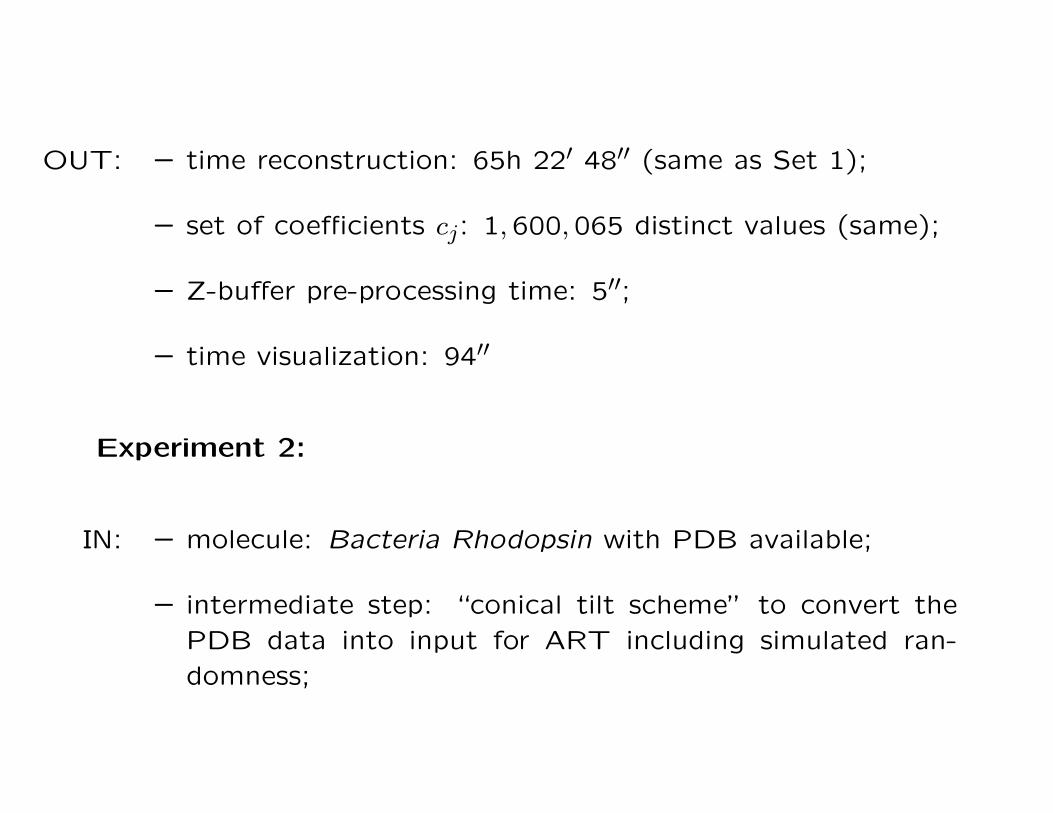
OUT: – time reconstruction: 65h 22′ 48′′ (same as Set 1);

– set of coefficients cj: 1,600,065 distinct values (same);

– Z-buffer pre-processing time: 5′′;

– time visualization: 94′′

Experiment 2:

IN: – molecule: Bacteria Rhodopsin with PDB available;

– intermediate step: “conical tilt scheme” to convert the

PDB data into input for ART including simulated ran-

domness;

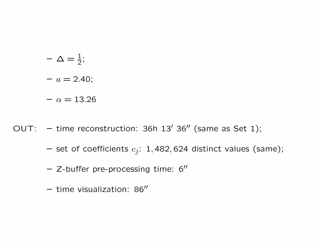
– ∆ = 12;

– a = 2.40;

– α = 13.26

OUT: – time reconstruction: 36h 13′ 36′′ (same as Set 1);

– set of coefficients cj: 1,482,624 distinct values (same);

– Z-buffer pre-processing time: 6′′

– time visualization: 86′′

Conclusion

Through careful use of various improvements to the implicit sur-

face intersection search algorithm, a substantial speed-up in vi-

sualization times for data which has already been reconstructed

can be achieved (about 60 times, from hours to only seconds),

bringing such visualizations into the speed range where multiple

views and even interactive exploration become possible.