http://www.unece.org/env/lrtap/WorkingGroups/wge/welcome.html

REPORT BY THE WORKING GROUP ON EFFECTS

Impacts of air pollution on ecosystems, human health and materials under

different Gothenburg Protocol scenarios

Cover photos (courtesy of ICPs):

Arc de triomphe du Carrousel, Paris

Ekso, a limed river, Norway

Wheat in Picardie, France

Spring in Halatte Forest, France

i

EXECUTIVE SUMMARY The objectives of this analysis, decided by the Bureau of the Working Group on Effects, are to:

• Provide information on the effects of air pollution on ecosystems, human health and materials to support decisions for the revision of the Gothenburg Protocol.

• Demonstrate the application of new science and indicators, developed since 1999, to illustrate the potential impact of policy /decisions on the environment, human health and materials.

• Illustrate the effectiveness of emission reductions scenarios to improve the environment and human health.

This analysis has been carried out by the International Cooperative Programmes (ICPs) and Task Force on Health under the Working Group on Effects (WGE) between October 2010 and December 2011. The analysis is based on scenarios of air pollutant (sulphur, nitrogen and particulate matter) and precursor emissions (ozone,O3) provided by the Task Force on Integrated Assessment Modelling (TFIAM) and the European Monitoring and Evaluation Programme (EMEP). A first draft was based on data available in October 2010 and described in CIAM report 1/2010 (Amann et al, 2010). The present document is an update based on scenarios published by IIASA in August 2011 (described in CIAM report 4/2011, Amann et al, 2011). The update reflects the discussions during the various phases of the negotiations of the Gothenburg Protocol revision. Relevant data was formatted by the Coordination Centre for Effects (CCE) in order to facilitate the ICPs modelling work and comparison with field data.

Results have been presented and discussed at different meetings under the Long-range Transboundary Air Pollution Convention (LRTAP) in 2011.

The scenarios and projections referred to in this report are:

• NAT2000: historical data for the year 2000 based mainly on national information.

• COB2020: Cost Optimised Baseline for the year 2020. This dataset is generated assuming that only current (2011) legislation still apply in 2020.

• Low*2020, MID2020 and High*2020: These are generated assuming increasing ambition levels for environmental targets.

• MTFR2020: data based on a scenario assuming that all technically feasible technologies are implemented by 2020.

The baseline activity data on energy use, transport, and agricultural activities were issued from different sources, including national submissions to IIASA and from specialized sectorial energy, transport and agricultural models (e.g., PRIMES, TREMOVE and CAPRI). They were then used as input data for the GAINS model with which scenarios were optimised so that emissions control scenarios would achieve environmental targets for human health and environmental impacts (acidification, eutrophication, effect of ground-level ozone) as discussed in the 48th session of the WGSR. MTFR represents the reduction that would be obtained if the most stringent regulations were implemented. Any decision leading to some emission reduction will lead to a situation between the baseline and the MTFR scenario. The low*, MID and high* scenarios are representing 3 of these possible situations. Further details on these projections and scenarios are specified in CIAM reports 1/2010 and 4/2011 (Amann et al., 2011a, b).

ii

Deposition trends

Air pollution regulations, including protocols of the LRTAP Convention, have led to significant decreases in sulphur and nitrogen concentrations in the air and in their deposition to ecosystems. The trends show that the sulphur dioxide emissions in Europe have decreased by more than 70% in 2010 compared to 1980 while total nitrogen emissions have decreased by about 50% in the same period (Figure 1). The consequences of these decreased emissions have been observed through the monitoring network designed under the LRTAP Convention and this report illustrates some of the results.

1880 1900 1920 1940 1960 1980 2000 2020

10

20

30

40

50

60

70

Mt/y

r of

SO

2, N

O2,

NH

3

Figure 1: 1880–2030 development of European emissions of S (solid line), oxidized N (dashed line) and reduced N (dashed-dotted line). Baseline scenarios for 2000 and 2020 are represented with thick lines. The thin lines point to the MTFR scenario for 2020.

Impacts

The Working Group on Effects has, over several decades, developed, compiled and collated a large amount of multidisciplinary scientific knowledge related to the impact of air pollution on ecosystems, human health and materials. The monitoring and modelling carried out by the ICPs1 and Task Forces enable analysis of the dynamics and trends of biotic and abiotic parameters of ecosystems. Selected examples illustrate the impacts of the increase and decrease of air pollution on the environment. More results are available on the WGE and ICPs/TF web sites as well as in the scientific literature.

The monitoring and the modelling carried out under the Working Group on Effects shows that the magnitude of the impact of air pollution will decrease under baseline (COB2020) and MTFR scenarios. However, as illustrated and summarized below, none of the impacts considered (eutrophication, effects of ozone, acidification, material soiling and corrosion, human health effects) are expected to disappear by 2020 under any scenario.

Eutrophication

Eutrophication will remain a widespread problem. In terrestrial ecosystems, excesses of nitrogen inputs leads to accumulation of nitrogen in soils and eventually its leaching to waters. This can promote a decline in species diversity and enhance the susceptibility of

1 International Cooperative Programmes. The Working Group on Effects is built on 6 ICPs and one Task Force (TF), each have a specific area of interest.

iii

vegetation to insects, fungal diseases or drought. Calculations from ICP Modelling and Mapping were supported by assessments from ICP Integrated Monitoring and ICP Forests: in 2020, under the baseline scenario, 59% of EU27 and 37% of European areas are estimated to be still at risk of eutrophication. The amplitude of the calculated nitrogen exceedances will range between 3 and 5 kg ha-1 yr-1 at ICP Integrated Monitoring sites which are situated in background areas distant from local sources. Also, under baselines projections, the proportion of eutrophic (C:N between 10-17) and hypertrophic (C:N smaller than 10) sites is expected to continue to increase at ICP Forests monitoring sites beyond 2020. Observations at ICP Integrated Monitoring sites show evidence for correlations between critical loads exceedances calculated with the NAT2000 scenario and measured parameters characterising acidification and eutrophication. This confirms the robustness of the critical loads methodology.

The contribution of ammonia to ecosystem damage is expected to remain important across Europe under the baseline scenario. In 2020, ammonia critical levels for bryophytes and higher plants will be exceeded in intensive agriculture areas (western France, The Netherlands and northern Italy) whereas ammonia will contribute to eutrophication over most areas in Europe. This contribution will be the greatest where critical levels are exceeded.

Acidification

ICP Modelling and Mapping results suggest that acidification will be of concern in 1 to 4% of the European area. This is consistent with the results from ICP Forests, ICP Waters and ICP Integrated Monitoring, whose observations and modelling show that most monitored sites are recovering from acidification except that the most acidified sites which will not recover by 2020, even under MTFR. Moreover, a tendency towards low base cation saturation in forests soils is expected. In the long term, this may have deleterious consequences on the soil nutritional status as well as on the base cations supply to fresh waters.

Ozone

Ozone affects human health, forests, grasslands, crops and contributes to corrosion of materials. Ecosystems in southern Europe are at particular risk of ozone impacts, but areas at risk also include most central and western parts of Europe. ICP Vegetation has shown that ozone pollution may partly suppress the terrestrial carbon sink via its adverse effects on plant growth, poses a threat to food security by reducing yield and quality and can also make vegetation less able to withstand periods of drought. Projected air pollution reductions may lead to lower ozone concentrations but, under the COB2020 baseline scenario, for example, wheat yield losses may still be greater than 5% in more than 80% of the EMEP grid squares. The Task Force on Health showed that currently in the EU25 there are 21,000 premature deaths every year due to high ozone concentrations (>35 ppb or 70 µg/m3). Only a small decrease in the number of premature deaths is expected with the full implementation of the current legislation.

Particulate matter

Particulate matter (PM) causes respiratory and cardiovascular mortality and morbidity and over 300,000 premature deaths are attributed to them every year in Europe. In the US, a recent study demonstrated that health improvement was associated with the decrease of PM levels over 20 years. In this study, a 7.3 months increase in life expectancy was attributed to a decrease of PM2.5 by 10 µg/m3. The Task Force on Health has compared the health risk associated with black carbon to that associated with PM2.5. They concluded that although there is sufficient evidence of health risk associated with black carbon, it is insufficient to justify replacing PM2.5 by black carbon as a health-relevant indicator of particulate air pollution.

iv

Particulate matter and other air pollutants also cause soiling and corrosion, which damage building materials and cultural heritage buildings. ICP Materials have established dose-response relationships and proposed targets for 2020 and 2050. These targets correspond to tolerable levels of corrosion or soiling. For instance, the proposed tolerable level for soiling results in PM10 levels less than 20 µg/m3 for 2020 and less than 10 µg/m3 for 2050. Calculations carried out at the scale of the EMEP grid (50x50 km²) suggest that with the baseline scenario, the more stringent 2050 targets would be achieved on nearly 83% of the European area, while on almost all of the remaining 17% the 2020 targets would be achieved by 2050. Comparisons with field data, however, show that these calculations are too optimistic and that urban areas are pollution hotspots which are likely to remain at higher risk than shown at the 50x50 km² grid scale used in this assessment.

Economic impacts and impacts on ecosystem services

Currently economic impact assessments are performed in the GAINS model only for human health indicators. However, several of the ICPs are developing their work towards associating the impacts described above to ecosystem services or economic costs, or both. Recent data from ICP Vegetation suggests economic losses amounted to more than three billion euros in 2000, due to ozone damage to Europe’s most extensively grown crop, wheat. ICP Materials indicators may also be associated with specific costs in the future. Impacts on air pollution on ecosystems may be evaluated, in terms of availability of drinking water, resilience of forests to pest attack, to drought (which may have a cost in term of wood quality), and quality of recreational areas (with, for instance, impacts on recreational fisheries).

In summary, even though a full (hypothetical) implementation of the MTFR scenario for 2020 would lead to improvements in human health and state of ecosystems, many areas would remain at risk from the adverse impacts of air pollution on ecosystems (including crops), human health and materials. Thanks to air pollution regulations implemented since the 1980s, acidification will be of least concern in the future. However, considerable adverse impacts of eutrophication (nitrogen pollution), ozone and particulate matter (including black carbon) will remain over large areas of Europe. The scenario analysis of impacts clearly shows that the higher the ambition of the emission reduction the greater the environmental and health benefits.

v

CONTENTS

EXECUTIVE SUMMARY ......................................................................................... I

LIST OF FIGURES ................................................................................................ VI

LIST OF TABLES .................................... ........................................................... VIII

GLOSSARY .......................................... ................................................................ IX

Acronyms .............................................................................................................. ix

Definitions .............................................................................................................. x

1. INTRODUCTION AND AIMS ............................. .............................................. 1

2. SCENARIOS .................................................................................................... 2

3. ICPS AND TASK FORCE RESULTS ....................... ....................................... 3

3.1 ICP Forests: Eutrophication and acidification in forests ................................ 3

3.2 ICP Waters: Recovery from acidification of surface waters .......................... 8

3.3 ICP Integrated Monitoring: Eutrophication and acidification of forested catchments ................................................................................................. 15

3.3.1 Assessments of critical loads at ICP IM sites ........................................... 15

3.3.2 Comparison of exceedance of critical loads with empirical effects indicators ................................................................................................................. 16

3.4 ICP Modelling and Mapping: Eutrophication, acidification, biodiversity changes at European scale ....................................................................................... 19

3.4.1 Accumulated Average Exceedances and Areas at risk of acidification and eutrophication .......................................................................................... 19

3.4.2 Risks of significant change in plant biodiversity ....................................... 23

3.4.3 Robustness analysis ................................................................................ 25

3.5 ICP Vegetation: Ozone impacts on vegetation and crops .......................... 26

3.5.1 Background .............................................................................................. 26

3.5.2 Policy-relevant effect indicators ............................................................... 27

3.5.3 Mapping different effect indicators using the various projections ............. 27

3.5.4 Temporal trends ....................................................................................... 31

3.5.5 Ozone impacts in a changing climate beyond 2050 ................................. 31

3.6 ICP Materials: Corrosion and soiling of building materials including cultural heritage ...................................................................................................... 32

3.7 Task Force on health .................................................................................. 35

4. DISCUSSION AND CONCLUSIONS ........................ ..................................... 36

4.1 Policy successes monitored by the Working Group on Effects ................... 36

4.2 Scientific knowledge: State of the art .......................................................... 37

4.3 On-going effect based scientific studies to support the LRTAP Convention 39

4.4 Overall conclusion ...................................................................................... 40

5. BIBLIOGRAPHY ...................................... ...................................................... 41

vi

LIST OF FIGURES Figure 1: 1880–2030 development of European emissions of S (solid line), oxidized N (dashed line) and

reduced N (dashed-dotted line). Baseline scenarios for 2000 and 2020 are represented with thick lines.

The thin lines point to the MTFR scenario for 2020. ................................................................................ ii

Figure 2: 1880–2030 development of European emissions of S (solid line), oxidized N (dashed line) and

reduced N (dashed-dotted line). Baseline scenarios for 2000 and 2020 are represented with thick lines.

The thin lines point to the MTFR scenario for 2020. ................................................................................ 1

Figure 3: Exceedances of critical loads for acidity resulting from the scenarios EMEP1980 (a), NAT2000 (b),

COB2020 (c), Low*2020 (d), High*2020 (e), and MTFR2020 (f) ................................................................ 4

Figure 4: The exceedance of critical loads for nutrient nitrogen resulting from the scenarios EMEP1980 (a),

NAT2000 (b), COB2020 (c), Low*2020 (d), High*2020 (e), and MTFR2020 (f) .......................................... 5

Figure 5: Overall trend for base saturation classes modelled by VSD+ for 77 plots in Europe assuming future

deposition according to the COB2020 scenario. ...................................................................................... 6

Figure 6: Overall trend for pH value modelled by VSD+ and classified by buffering classes (Ulrich 1981) for 77

plots in Europe assuming future deposition according to the COB2020 scenario. ................................... 7

Figure 7: Overall trend for C:N ratio modelled by VSD+ and classified by nutrient levels for 77 plots in Europe

assuming future deposition according to the COB2020 scenario. ............................................................ 8

Figure 8: Long-term deposition, lake chemistry and lake biology monitoring data for Lake Saudlandsvatn, an

ICP Waters site in southern Norway. Shown are non-marine S (S*) deposition, lake ANC and pH, catch-

per-unit effort of fish, number of specimens collected of the acid-sensitive mayfly B. rhodani, and %

specimens collected of the acid-sensitive zooplankton species D longispina (Data from Hesthagen et al.

2011). ...................................................................................................................................................... 9

Figure 9: Concentrations of sulphate (SO4) and ANC in Lake Saudlandsvatn measured (red squares) and

simulated (blue lines) with the MAGIC model. The future simulated values assume S* deposition as

specified by the COB2020 scenario with linear decrease from 2000 to 2020 and constant level past the

year 2020. ............................................................................................................................................. 10

Figure 10: Non-marine S deposition, nitrogen deposition (NOx + Nred), and simulated and observed acid

neutralising capacity (ANC) at Lake Saudlandsvatn, southern Norway. Three deposition scenarios are

presented: COB2020, MTFR2020 and background (bkgd). The background deposition scenario was

included to illustrate the maximum theoretical additional improvement in water quality towards which

ecosystems are expected to tend to in absence of sulphur and nitrogen pollution. Also shown are the

annual observed ANC concentrations (squares). ................................................................................... 11

Figure 11: Locations of the 8 ICP Waters sites used with the MAGIC model for the current assessment. ....... 12

Figure 12: Simulated and observed acid neutralising capacity (ANC) at each of the 8 ICP Waters sites. Three

deposition scenarios are presented: COB2020 (current legislation, including the Gothenburg Protocol),

MTFR2020 (maximum feasible reduction) and bkgd (background deposition only). The background

deposition scenario was included to illustrate the maximum theoretical additional improvement in

water quality towards which ecosystems are expected to tend in absence of S and N pollution. See

Table 2 for site details. .......................................................................................................................... 13

Figure 13: Modelled ANC (µeq/l) in years 2000 and 2030 under the five scenarios for the Gothenburg

Protocol revision and associated sulphur and nitrogen deposition. Values are given for the year 2030,

which allows the ecosystems 10 years to respond after the revised protocol implementation year in

2020. Bars in the red areas imply that the lake is acidified, bars in the green area indicate lakes not

acidified whereas the yellow area indicates situations where lakes are still at risk of acidification....... 14

Figure 14: Number of plots in ICP IM sites that are protected/not protected from eutrophication (according

to calculations based on empirical critical loads) assuming different deposition scenarios. .................. 16

Figure 15 : Exceedance of critical load for acidification (ExCLA NAT2000 scenario, x-axis) for aquatic

ecosystems vs. annual mean concentrations (left column) and fluxes (right column) measured between

2000 and 2002 (y-axis) of ANC and H+ in runoff for 17 ICP IM sites. Negative exceedance values included

in graphs represent non-exceedance of critical loads. ........................................................................... 17

vii

Figure 16: Exceedance of critical load for mass balance nutrient nitrogen (ExCLnutN, x-axis) vs. mean annual

fluxes (left down) and concentrations (left upper) (2000-2002) (y-axis) of TIN (NO3+NH4) in runoff for 16

to 18 ICP IM sites, and exceedance of empirical values of critical load for nutrient nitrogen (ExCLempN,

eq ha-1

yr-1

x-axis) vs. mean annual fluxes (right down) and concentrations (right up) (2000-2002) (y-axis)

of TIN (NO3+NH4) in runoff for 16-24 ICP IM sites. Exceedance values were calculated using the

NAT2000 deposition scenario. Negative exceedance values included in graphs represent non-

exceedance of critical loads. The sites with a significant input of N from sources other than deposition

are denoted with a lighter green circle. ................................................................................................. 18

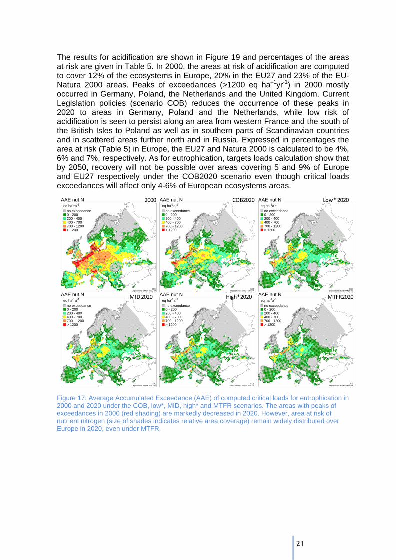
Figure 17: Average Accumulated Exceedance (AAE) of computed critical loads for eutrophication in 2000 and

2020 under the COB, low*, MID, high* and MTFR scenarios. The areas with peaks of exceedances in

2000 (red shading) are markedly decreased in 2020. However, area at risk of nutrient nitrogen (size of

shades indicates relative area coverage) remain widely distributed over Europe in 2020, even under

MTFR..................................................................................................................................................... 21

Figure 18 : Average Accumulated Exceedance (AAE) of empirical critical loads of nutrient N in 2000 (left), in

2020 under the COB (centre) and MID (right) scenarios. The areas where exceedances occur in 2000

(colour shading) are markedly decreased in 2020 compared to 2000. ................................................... 22

Figure 19: Average Accumulated Exceedance (AAE) of critical loads for acidification in 2000 and 2020 under

the COB, low*, MID, high* and MTFR scenarios. Peaks of exceedances in 2000 on the Dutch-German

border and in Poland (red shading) are reduced in 2020, as is the area at risk in general (more grey

cells). ..................................................................................................................................................... 22

Figure 20 : Areas at risk of the exceedance of the critical level for ammonia in 2020 under the COB (top left)

and MID (bottom left) scenarios in comparison to the areas at risk of the exceedance by the deposition

of ammonium of the critical load of nutrient N under the COB (top right) and MID scenarios. ............. 23

Figure 21: The location of natural areas (covering about half, i.e. about 2 million km2, of the European natural

area characterised by the EUNIS classification) where the computed change of biodiversity is higher

than 5% (red shading) in 2000 (top-left) and in 2020 under the COB (top-centre), low* (top-right), MID

(bottom-left), high* (bottom-centre) and MTFR (bottom-right) scenarios. ........................................... 24

Figure 22 : The likelihood that exceedance (computed as AAE) is ‘virtually certain’ (red shading), i.e. that a

grid cell contains at least one ecosystem of which the critical load of nutrient N is exceeded in 2000

(top left), CLE (top centre), Low* (top right), MID (bottom left), High* (bottom centre) and MFR

(bottom right). ...................................................................................................................................... 25

Figure 23: The risk of adverse ozone impacts in 2000 a) on biomass production in forest as indicated by the

concentration-based AOT40 for forest trees (the AOT40-based critical level is 5 ppm.h), b) on human

health as indicated by SOMO35, c) on generic deciduous tree as calculated by the flux model (POD1).

The maps were produced using the NAT 2000 projection. .................................................................... 28

Figure 24: The risk of adverse ozone impacts in 2020 on biomass production in forest using the generic

deciduous tree flux model (POD1) for a) COB2020, b) MID2020, c) MTFR2020. ..................................... 28

Figure 25: Proportion of grid squares within specified categories of POD1 calculated using the generic forest

flux model as calculated with the different datasets. ............................................................................ 29

Figure 26: Predicted economic losses for ozone effects on wheat in millions € per 50 x 50 km grid square in

(a) 2000 and (b) 2020 for the wheat growing areas of EU27+CH+NO as indicated by the NAT scenario

and flux-based methodology (from Mills and Harmens, 2011). ............................................................. 30

Figure 27: Predicted economic losses for effects on tomato in millions € per 50 x 50 km grid square in (a) 2000

and (b) 2020 for the tomato growing areas of EU27+CH+NO (> 1 t yield per square) as indicated by the

NAT scenario and flux-based methodology (from Mills and Harmens, 2011). ....................................... 30

Figure 28 : Combined indicator for materials based on individual targets for the indicators carbon steel, zinc

and limestone corrosion, and soiling. .................................................................................................... 34

viii

LIST OF TABLES Table 1 : Environmental and human health targets for the scenarios Low*, MID and High*, set as percentage

of the gap closure between the effects expected for the COB2020 scenario (0% gap closure) and the

MTFR2020 scenario (100%gap closure) (further details in Amann et al., 2011a, b). ................................ 2

Table 2: Locations of the 8 ICP Waters sites used for the assessment of the different projections. ................ 12

Table 3 : Summary of biological status in the study lakes observed (1980, 2000, 2010) and forecast recovery

under two scenarios for 2020. Recovery classes: 0 no recovery; * start recovery; ** partial recovery;

*** full recovery. NS= not studied......................................................................................................... 14

Table 4: Average exceedance of critical loads for acidification CLA and eutrophication CLnutN and CLempN at ICP

IM sites according to the Gothenburg Protocol scenarios. .................................................................... 16

Table 5: Areas at risk of acidification and eutrophication in Europe according to the 5 scenarios tested for the

revision of the Gothenburg Protocol. All % refer to the EU27 or European areas where calculated

critical loads are exceeded. ................................................................................................................... 19

Table 6 : The percent area for which target loads are exceeded that would be required for achieving recovery

from eutrophication and acidification in 2050, according to the COB and MID scenarios. ..................... 20

Table 7: The percent area at risk in 2000, and in 2020 under the five scenarios, of a change by more than 5%

in biodiversity, i.e. of the species richness of (semi-) natural grasslands (EUNIS class E) and arctic and

(sub-)alpine scrub habitats (EUNIS class F2) and of the Sorensen similarity index of the understorey

vegetation of coniferous boreal woodlands (EUNIS class G3 A-C). ........................................................ 25

Table 8 : Percentages of the area at risk of acidification and eutrophication as computed in support of policy

processes in the 48th

session of the Working Group on Strategies and Review (WGSR48) in the spring of

2011, in comparison to those submitted to the WGSR49. ..................................................................... 26

Table 9 : Predicted impacts of ozone pollution on wheat and tomato yield and economic value, together with

critical level exceedance in EU27+Switzerland+Norway in 2000 and 2020 under the current legislation

scenario (NAT scenario). Analysis was conducted on a 50 x 50 km EMEP grid square using crop values in

2000 and an ozone stomatal flux-based risk assessment (From Mills and Harmens, 2011). .................. 31

Table 10: Targets for protecting materials of infrastructure and cultural heritage for 2020 and 2050

(ECE/EB.AIR/WG.1/2009/16 “Indicators and targets for air pollution effects”) ..................................... 33

Table 11 : Compliances of targets of indicators for materials calculated from dose-response relationships for

the whole EUROPEAN region in 2020. ................................................................................................... 33

Table 12: Comparison of field observations of atmospheric SO2 concentrations and corrosion of carbon steel,

zinc and limestone at ICP Materials test sites for the year 2000 (“Field”) and values for the same

parameters calculated from the NAT 2000 dataset (“Nat”) for the corresponding grid cells. ................ 35

ix

GLOSSARY

ACRONYMS AAE Average Accumulated Exceedance of a critical load

ACS American Cancer Society

ANC Acid neutralising capacity. Defined as equivalent sum of base cations (Ca, Mg, Na, K) minus

equivalent sum of strong acid anions (SO4, Cl, NO3). Units: µeq/l. ANC is a measure of degree

of acidification of water.

ANClimit The lowest ANC concentration that does not damage an indicator organism

AOT40 Accumulated ozone dose over the threshold of 40ppb

CCE Coordination Centre for Effects

CIAM Centre for integrated assessment modelling at the International Institute for Applied System

Analysis (Austria)

CLA Critical load of acidity

CLempN Empirical critical loads of nutrient nitrogen

CLnutN Critical load of nutrient nitrogen

CLe Critical level

EMEP Cooperative Programme for Monitoring and Evaluation of the Long-range Transmission of Air

Pollutants in Europe

EUNIS European nature information system (i.e. classification of ecosystems)

FAB First order acidity balance (model)

GAINS Greenhouse gas – Air pollution Interactions and Synergies model

HIA Health Impact Assessment

ICP International Cooperative Programme

LRTAP (Convention on) Long-range Transboundary Air Pollution

MAGIC Model for Acidification of Groundwater In Catchments

MTFR Maximum technically feasible reduction

NAT Emission scenario based on data provided by each party (national data)

NOx Oxidised forms of reactive nitrogen

Nred Reduced forms of reactive nitrogen

PODY Phytotoxic ozone dose above a flux threshold of Y nmol m2ـ

s1ـ

PRIMES Energy Systems Model of the National Technical University of Athens

S* Non-marine sulphur

SMB Simple Mass Balance (model)

SSWC Steady-State Water Chemistry (model)

TFIAM Task Force on Integrated Assessment Modelling

WGE Working Group on Effects under the Convention on Long-range Transboundary Air Pollution

WGSR Working Group on Strategies and Review under the Convention on Long-range

Transboundary Air Pollution

x

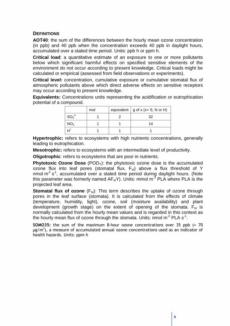
DEFINITIONS AOT40: the sum of the differences between the hourly mean ozone concentration (in ppb) and 40 ppb when the concentration exceeds 40 ppb in daylight hours, accumulated over a stated time period. Units: ppb h or ppm h. Critical load : a quantitative estimate of an exposure to one or more pollutants below which significant harmful effects on specified sensitive elements of the environment do not occur according to present knowledge. Critical loads might be calculated or empirical (assessed from field observations or experiments). Critical level: concentration, cumulative exposure or cumulative stomatal flux of atmospheric pollutants above which direct adverse effects on sensitive receptors may occur according to present knowledge. Equivalents: Concentrations units representing the acidification or eutrophication potential of a compound.

mol equivalent g of x (x= S, N or H)

SO42- 1 2 32

NO3- 1 1 14

H+ 1 1 1

Hypertrophic: refers to ecosystems with high nutrients concentrations, generally leading to eutrophication. Mesotrophic: refers to ecosystems with an intermediate level of productivity. Oligotrophic : refers to ecosystems that are poor in nutrients. Phytotoxic Ozone Dose (PODY): the phytotoxic ozone dose is the accumulated ozone flux into leaf pores (stomatal flux, Fst) above a flux threshold of Y nmol m2ـ s1ـ, accumulated over a stated time period during daylight hours. (Note this parameter was formerly named AFstY). Units: mmol m-2 PLA where PLA is the projected leaf area. Stomatal flux of ozone (Fst): This term describes the uptake of ozone through pores in the leaf surface (stomata). It is calculated from the effects of climate (temperature, humidity, light), ozone, soil (moisture availability) and plant development (growth stage) on the extent of opening of the stomata. Fst is normally calculated from the hourly mean values and is regarded in this context as the hourly mean flux of ozone through the stomata. Units: nmol m-2 PLA s-1.

SOMO35: the sum of the maximum 8-hour ozone concentrations over 35 ppb (= 70 µg/m3), a measure of accumulated annual ozone concentrations used as an indicator of health hazards. Units: ppm h

1

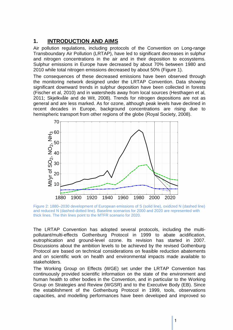
1. INTRODUCTION AND AIMS Air pollution regulations, including protocols of the Convention on Long-range Transboundary Air Pollution (LRTAP), have led to significant decreases in sulphur and nitrogen concentrations in the air and in their deposition to ecosystems. Sulphur emissions in Europe have decreased by about 70% between 1980 and 2010 while total nitrogen emissions decreased by about 50% (Figure 1). The consequences of these decreased emissions have been observed through the monitoring network designed under the LRTAP Convention. Data showing significant downward trends in sulphur deposition have been collected in forests (Fischer et al, 2010) and in watersheds away from local sources (Hesthagen et al, 2011; Skjelkvåle and de Wit, 2008). Trends for nitrogen depositions are not as general and are less marked. As for ozone, although peak levels have declined in recent decades in Europe, background concentrations are rising due to hemispheric transport from other regions of the globe (Royal Society, 2008).

1880 1900 1920 1940 1960 1980 2000 2020

10

20

30

40

50

60

70

Mt/y

r of

SO

2, N

O2,

NH

3

Figure 2: 1880–2030 development of European emissions of S (solid line), oxidized N (dashed line) and reduced N (dashed-dotted line). Baseline scenarios for 2000 and 2020 are represented with thick lines. The thin lines point to the MTFR scenario for 2020.

The LRTAP Convention has adopted several protocols, including the multi-pollutant/multi-effects Gothenburg Protocol in 1999 to abate acidification, eutrophication and ground-level ozone. Its revision has started in 2007. Discussions about the ambition levels to be achieved by the revised Gothenburg Protocol are based on technical considerations on feasible reduction abatements and on scientific work on health and environmental impacts made available to stakeholders. The Working Group on Effects (WGE) set under the LRTAP Convention has continuously provided scientific information on the state of the environment and human health to other bodies in the Convention, and in particular to the Working Group on Strategies and Review (WGSR) and to the Executive Body (EB). Since the establishment of the Gothenburg Protocol in 1999, tools, observations capacities, and modelling performances have been developed and improved so

2

that it is now possible to provide a comprehensive overview of the state of the environment and human health and to forecast changes to come. This WGE report describes the results of the analysis of impacts obtained with new and updated indicators for emission projections supplied by the Centre of Integrated Assessment Modelling (CIAM) in August 2011. It should be seen as complementary to the information provided by GAINS and reported in CIAM’s reports (Amann et al., 2011a, b; Amann et al., 2010).

2. SCENARIOS The “Gothenburg Protocol revision scenarios” referred to in this report are:

• NAT2000: historical data for the year 2000 based mainly on national information.

• COB2020: Cost Optimised Baseline for the year 2020. This dataset is generated assuming that only current (2011) legislation still apply in 2020.

• MTFR2020: data based on a scenario assuming all technically feasible technologies being implemented by 2020.

• Low*2020, MID2020, High*2020: Scenarios with increasing ambitions for environmental and human health targets as described in Table 1.

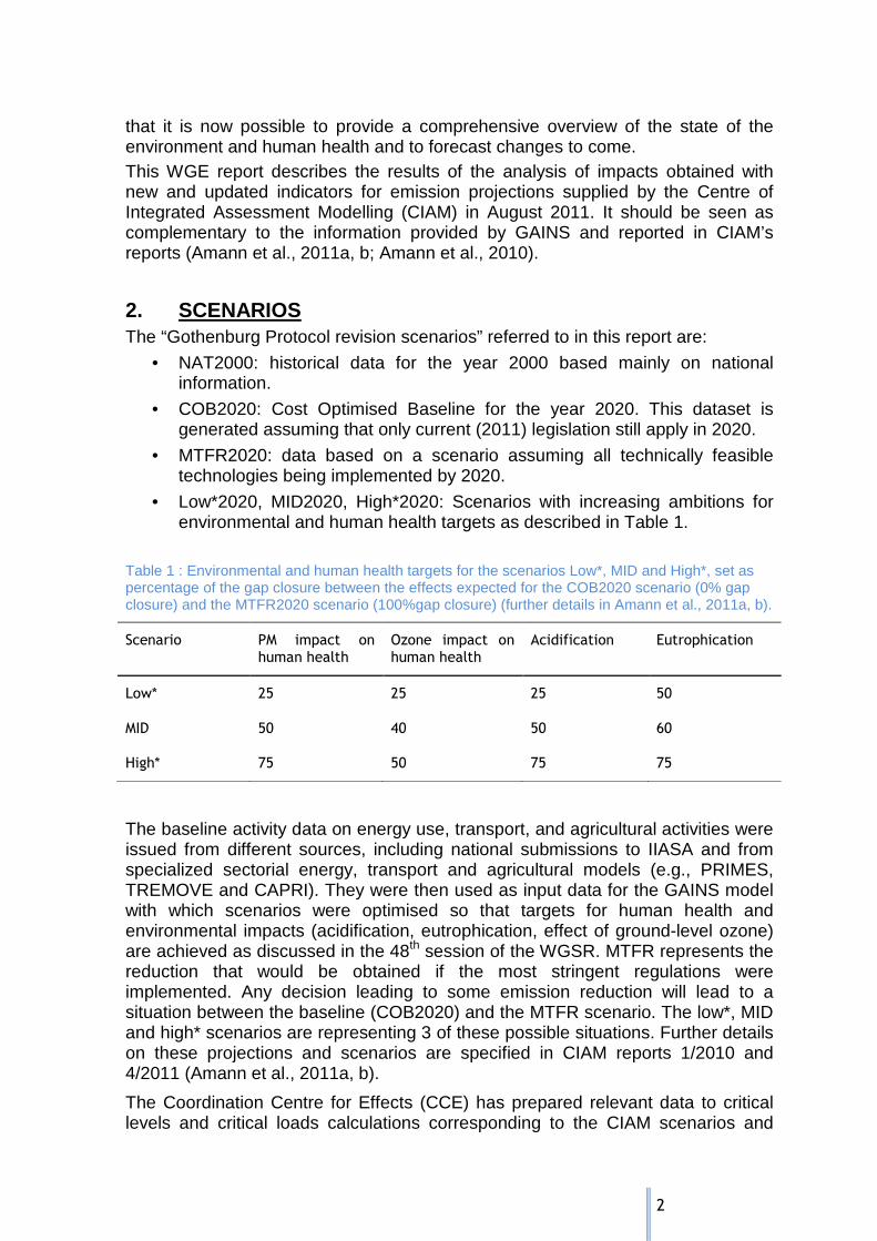
Table 1 : Environmental and human health targets for the scenarios Low*, MID and High*, set as percentage of the gap closure between the effects expected for the COB2020 scenario (0% gap closure) and the MTFR2020 scenario (100%gap closure) (further details in Amann et al., 2011a, b).

Scenario PM impact on human health

Ozone impact on human health

Acidification Eutrophication

Low* 25 25 25 50

MID 50 40 50 60

High* 75 50 75 75

The baseline activity data on energy use, transport, and agricultural activities were issued from different sources, including national submissions to IIASA and from specialized sectorial energy, transport and agricultural models (e.g., PRIMES, TREMOVE and CAPRI). They were then used as input data for the GAINS model with which scenarios were optimised so that targets for human health and environmental impacts (acidification, eutrophication, effect of ground-level ozone) are achieved as discussed in the 48th session of the WGSR. MTFR represents the reduction that would be obtained if the most stringent regulations were implemented. Any decision leading to some emission reduction will lead to a situation between the baseline (COB2020) and the MTFR scenario. The low*, MID and high* scenarios are representing 3 of these possible situations. Further details on these projections and scenarios are specified in CIAM reports 1/2010 and 4/2011 (Amann et al., 2011a, b).

The Coordination Centre for Effects (CCE) has prepared relevant data to critical levels and critical loads calculations corresponding to the CIAM scenarios and

3

projections. The CCE then sent five datasets with N, S, O3 concentrations and depositions to ICPs in August 2011. The calculations presented in this report have been based on these data.

3. ICPS AND TASK FORCE RESULTS

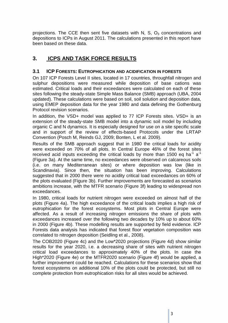
3.1 ICP FORESTS: EUTROPHICATION AND ACIDIFICATION IN FORESTS On 107 ICP Forests Level II sites, located in 17 countries, throughfall nitrogen and sulphur depositions were measured while deposition of base cations was estimated. Critical loads and their exceedances were calculated on each of these sites following the steady-state Simple Mass Balance (SMB) approach (UBA, 2004 updated). These calculations were based on soil, soil solution and deposition data, using EMEP deposition data for the year 1980 and data defining the Gothenburg Protocol revision scenarios. In addition, the VSD+ model was applied to 77 ICP Forests sites. VSD+ is an extension of the steady-state SMB model into a dynamic soil model by including organic C and N dynamics. It is especially designed for use on a site specific scale and in support of the review of effects-based Protocols under the LRTAP Convention (Posch M, Reinds GJ, 2009; Bonten, L et al. 2009). Results of the SMB approach suggest that in 1980 the critical loads for acidity were exceeded on 70% of all plots. In Central Europe 46% of the forest sites received acid inputs exceeding the critical loads by more than 1500 eq ha-1 a-1 (Figure 3a). At the same time, no exceedances were observed on calcareous soils (i.e. on many Mediterranean sites) or where deposition was low (like in Scandinavia). Since then, the situation has been improving. Calculations suggested that in 2000 there were no acidity critical load exceedances on 60% of the plots evaluated (Figure 3b). Further improvements are forecasted as scenarios ambitions increase, with the MTFR scenario (Figure 3f) leading to widespread non exceedances. In 1980, critical loads for nutrient nitrogen were exceeded on almost half of the plots (Figure 4a). The high exceedance of the critical loads implies a high risk of eutrophication for the forest ecosystems. Most plots in Central Europe were affected. As a result of increasing nitrogen emissions the share of plots with exceedances increased over the following two decades by 10% up to about 60% in 2000 (Figure 4b). These modelling results are supported by field evidence. ICP Forests data analysis has indicated that forest floor vegetation composition was correlated to nitrogen deposition (Seidling et al., 2008). The COB2020 (Figure 4c) and the Low*2020 projections (Figure 4d) show similar results for the year 2020, i.e. a decreasing share of sites with nutrient nitrogen critical load exceedances to approximately 40% of the plots. In case the High*2020 (Figure 4e) or the MTFR2020 scenario (Figure 4f) would be applied, a further improvement could be reached. Calculations for these scenarios show that forest ecosystems on additional 10% of the plots could be protected, but still no complete protection from eutrophication risks for all sites would be achieved.

4

Figure 3a Figure 3b

Figure 3c Figure 3d

Figure 3e Figure 3f

Figure 3: Exceedances of critical loads for acidity resulting from the scenarios EMEP1980 (a), NAT2000 (b), COB2020 (c), Low*2020 (d), High*2020 (e), and MTFR2020 (f)

5

Figure 4a Figure 4b

Figure 4c Figure 4d

Figure 4e Figure 4f

Figure 4: The exceedance of critical loads for nutrient nitrogen resulting from the scenarios EMEP1980 (a), NAT2000 (b), COB2020 (c), Low*2020 (d), High*2020 (e), and MTFR2020 (f)

It should be taken into account that critical loads data on which these exceedance calculations are based, are derived from steady-state mass balance methods, which are used to define long-term critical loads for systems at steady-state. Therefore, exceedance is an indication for the potential for harmful effects to

6

systems at steady-state, i.e. at some undefined time in the future. In order to evaluate how ecosystems evolve in time and eventually when recovery is possible, dynamic models are used. Here, they offer insight into the general development of soil solution chemistry which is dynamically reacting to changing deposition inputs. The dynamic model VSD+ was run on 77 plots across Europe assuming future depositions according to the COB2020 projection (Figure 5 to Figure 7). Based on differing site conditions the modelled trend for base saturation2 is heterogeneous. Nevertheless, a slight tendency towards dominance by low base saturation classes becomes visible. Statistical analysis of the model results suggests that most changes in base saturation occurred between 1960 and 2000 (Figure 5) when acidification was most widespread. In this period, the share of plots with low base saturation, i.e. below 20%, doubled from 10 to 20% of the observed plots, at the expense of the share of plots with a base saturation between 20 and 40%. After 2010, the model predicts hardly any changes on more than 90% of the plots. Model runs over longer time periods (not depicted) reveal similar results. The spatial analysis shows a tendency towards low base saturation for plots in central and eastern/north-eastern Europe, the region where acidification had been most pronounced.

Figure 5: Overall trend for base saturation classes modelled by VSD+ for 77 plots in Europe assuming future deposition according to the COB2020 scenario.

VSD+ calculations related to pH- as an indicator for acid deposition- also imply that major changes occurred between 1950 and 2000 (Figure 6). These changes include an increase in the share of plots with extremely low pH values in the 1970s and 1980s and a recovery from 1990 onwards. Most severe acidification was observed around the year 1980, when SO2 emission peaked. Between the years 2000 and 2050 there are hardly any changes visible on most of the plots. Results confirm that pH in soil solution is directly linked to increasing or decreasing acid deposition. Solid soil chemistry reacts much slower and its recovery can take decades (not depicted).

2 Base saturation is a measure of base cations availability. Base cations, such as calcium, magnesium or potassium are essential for vegetation growth.

7

Figure 6: Overall trend for pH value modelled by VSD+ and classified by buffering classes (Ulrich 1981) for 77 plots in Europe assuming future deposition according to the COB2020 scenario.

The carbon to nitrogen ratio (C:N) in soil solution is an indicator for the nitrogen status of the plots. Until 1970, the model predicts an increase in the share of nutrient poor plots (C:N > 24, see Figure 7) while the share of mesotrophic sites (C:N between 18 and 24) decreases. The eutrophic plots (C:N between 10 and 17) show an increasing trend since 1920. Starting in 1980, a clear trend towards more nutrient rich conditions is observed, indicated by shares of constantly increasing eutrophic and even hypertrophic plots. At the same time the share of plots with mesotrophic conditions shows no longer a clear trend but varies from one year to the next. The general increase in soil solution C:N ratios at the beginning of the observation period is attributed to a sharp increase in sulphur deposition at unchanged base cation and nitrogen supply. The resulting decrease in pH (see Figure 4) has probably led to reduced microbial activity in the soil and to an accumulation of carbon rich and slowly decomposing humus in the topsoil layer. But for several plots, another overlapping process needs to be considered. The fact that the supply with base cations in some regions was on a higher level at the beginning of the last century than today while simultaneously the nitrogen input was much lower might have led to a depletion of nutrient nitrogen. The increased nitrogen deposition starting in the middle of the 20th century put an end to nitrogen shortage and the reduced acidification at the end of the last century led to decomposition of previously accumulated organic matter. Decreasing C:N ratios clearly indicate the changed nutrient supply. Eutrophic conditions that are prevailing at the end of the observation period bear risks for the water filtering function of forest soils, may lead to shifts in species composition and are an indicator for nutrient imbalances that may destabilize forest ecosystems (Seidling et al., 2008).

8

Figure 7: Overall trend for C:N ratio modelled by VSD+ and classified by nutrient levels for 77 plots in Europe assuming future deposition according to the COB2020 scenario.

3.2 ICP WATERS: RECOVERY FROM ACIDIFICATION OF SURFACE WATERS ICP Waters assessed the effects of the deposition projections by means of the dynamic biogeochemical model MAGIC (Cosby et al. 1985, 2001). In the past, MAGIC has been extensively used to assess soil and water acidification, including a major assessment of the implementation of the Gothenburg Protocol (Wright et al. 2005). MAGIC provides an estimate of surface water acidification status (as indicated by the acid neutralising capacity; ANC) in response to a given scenario of S and N deposition over time. The resulting estimates of ANC were then used to evaluate biological response. There are robust dose-response relationships between ANC and key indicators of ecosystem damage, such as viable population of fish (brown trout, salmon), biodiversity of groups such as diatoms, invertebrates, and aquatic plants. These indicator organisms have been used to set critical limits (ANClimit), which in turn have been used to determine critical loads of acidity (CLA) (Henriksen and Posch, 2001). Lake Saudlandsvatn, southern Norway, provides a 35-year record that illustrates the rise and fall of acid deposition, acidification of water and damage and recovery to key biota (Hesthagen et al. 2011). At the start of the monitoring in 1974 the non-marine sulphur deposition (S*)3 greatly exceeded the critical load for acidity, the lake was acidified and had negative ANC (far below the ANClimit, the threshold below which damage is known to occur to the lake) and low pH (around 5 which is significantly below the natural background level of 5.5 – 6.0 from a biological point of view). Short-lived biological acid-sensitive indicator organisms (invertebrates and zooplankton) were absent and the native brown trout population was on its way to extinction. Since about 1988, S* deposition has decreased sharply, ANC and pH have increased and starting in the late 1990s the biota began to recover (Figure 8).

3 Marine aerosols contain significant quantities of sulphur. This natural sulphur may contribute to ecosystems acidification.

9

0

5

10

15

20

25

30

1974 1978 1982 1986 1990 1994 1998 2002 2006

% s

peci

men

s Zooplankton Daphnia longispina

0

10

20

30

40

50

no.

spe

cim

ens

Invertebrate Baetis rhodani

0

5

10

15

20

25

30

35

40

Cpu

e

Fish Salmo trutta

-40

-30

-20

-10

0

10

20

30

40

µeq

/l

ANC limit

lake ANC

0

50

100

150

200m

eq/m

2 /yr

CLA

S* deposition deposition

4.5

5.0

5.5

6.0

6.5

1974 1978 1982 1986 1990 1994 1998 2002 2006

pH

Figure 8: Long-term deposition, lake chemistry and lake biology monitoring data for Lake Saudlandsvatn, an ICP Waters site in southern Norway. Shown are non-marine S (S*) deposition, lake ANC and pH, catch-per-unit effort of fish, number of specimens collected of the acid-sensitive mayfly B. rhodani, and % specimens collected of the acid-sensitive zooplankton species D longispina (Data from Hesthagen et al. 2011).

At Lake Saudlandsvatn more than 90% of deposited N is retained in the lake and catchment and this situation has not changed during the 35 years of monitoring. Nitrogen deposition does not greatly affect lake acidification at least at present. Modelling focus can thus be placed on S* deposition.

MAGIC was first calibrated to the observed annual water chemistry data from the 1974-2009 period and driven by the historical sulphur and nitrogen deposition data for the EMEP grid square 50-57 provided by the CCE in the 2007-2008 call (Hettelingh et al., 2008). Since then emissions inventories, and subsequently deposition data, have been updated. In order to make use of the calibration carried out in 2008 with the presently available deposition data, it has been necessary to scale the deposition specified by the projection NAT2000 to the measured deposition at the site for the year 2000. The calibrated parameter set was then run with the five scenarios for deposition year 2020 of sulphur and nitrogen (projections COB2020, Low*2020, MID2020, High*2020, and MTFR2020). Deposition was assumed to decrease linearly from 2000 to 2020, and stay constant thereafter. ANC was used as the measure for acidification in the water. Projections were run through year 2050 to illustrate the long-term response to the changes in deposition.

The long-term reconstructed acidification history at Lake Saudlandsvatn suggests that ANC fell below the ANClimit for fish around 1950 and that ANC remained well below the ANClimit until recently (Figure 9). The year-to-year “noise” in ANC with present-day amplitude of about 30 µeq/l reflects natural variations in amounts of precipitation and sea salt inputs.

10

Saudlandsvatn SO4

COB2020 scenario

0

20

40

60

80

100

120

140

160

180

1850 1900 1950 2000 2050

µe

q/l

Saudlandsvatn ANC

COB2020 scenario

-60

-40

-20

0

20

40

60

80

100

1850 1900 1950 2000 2050

µe

q/l

ANClimit

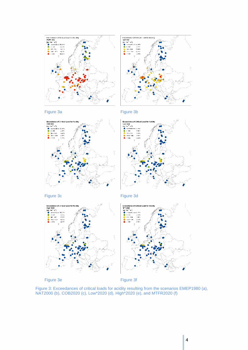
Figure 9: Concentrations of sulphate (SO4) and ANC in Lake Saudlandsvatn measured (red squares) and simulated (blue lines) with the MAGIC model. The future simulated values assume S* deposition as specified by the COB2020 scenario with linear decrease from 2000 to 2020 and constant level past the year 2020.

With the COB2020 projections, ANC levels are expected to continue to increase somewhat over the next 10 years, and then level off at about ANC 30 µeq/l. Year-to-year fluctuations, however, imply that ANC will fall below ANClimit during “bad” years, such as years with high sea salt inputs (Figure 9). The projected ANC for the year 2020 was almost the same with the five 2020 projections, with additional improvements for the MTFR2020 projection (Figure 10). This is because the future S* deposition is very similar under COB2020, Low*2020, MID2020, and High*2020 and somewhat less under MTFR2020. Therefore, only the COB2020 and MTFR2020 projections for ANC are shown in the following figures. To illustrate the maximum possible theoretical recovery, a scenario with only “background” deposition in the year 2020 and onwards was run. “Background” input here comprises volcanic emissions, di-methyl sulphide emissions from marine areas and fluxes from outside the EMEP modelled domain. This “background” scenario provides the theoretical upper limit towards which the ecosystems are expected to tend.

11

0

50

100

150

1990 2000 2010 2020 2030

me

q/m

2/yr

Saudlandsvatn, NO

S* deposition

COB2020

MFR2020

bkgd

0

50

100

150

200

1990 2000 2010 2020 2030

me

q/m

2/yr

Saudlandsvatn, NO

N deposition

COB2020

MFR2020

bkgd

-40

-30

-20

-10

0

10

20

30

40

1990 2000 2010 2020 2030µeq/

l

Saudlandsvatn, NO

lake ANC

COB2020

MFR2020

bkgd

obs

Figure 10: Non-marine S deposition, nitrogen deposition (NOx + Nred), and simulated and observed acid neutralising capacity (ANC) at Lake Saudlandsvatn, southern Norway. Three deposition scenarios are presented: COB2020, MTFR2020 and background (bkgd). The background deposition scenario was included to illustrate the maximum theoretical additional improvement in water quality towards which ecosystems are expected to tend to in absence of sulphur and nitrogen pollution. Also shown are the annual observed ANC concentrations (squares).

The same procedure was used to calibrate and run MAGIC with the scenarios at 8 acid-sensitive lakes in Europe (Figure 11, Table 2). These lakes are monitored as part of ICP Waters network.

12

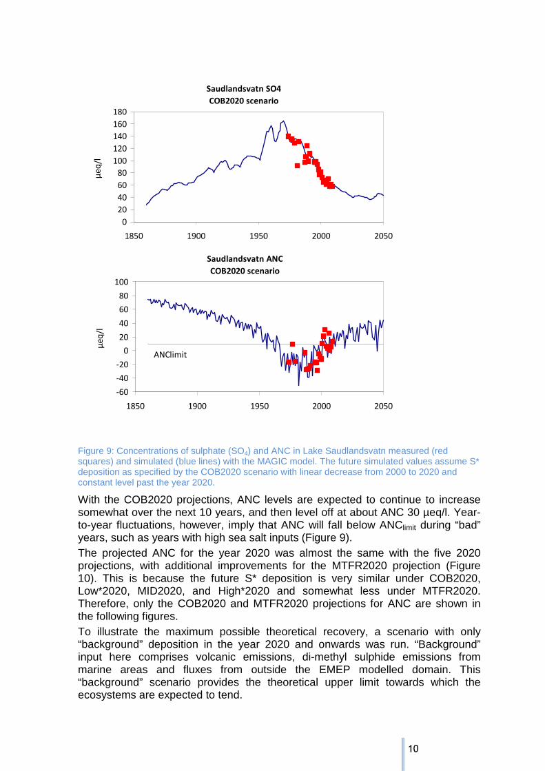
Table 2: Locations of the 8 ICP Waters sites used for the assessment of the different projections.

SITE COUNTRY LAT LONG EMEPi EMEPj REFERENCE

Saudlandsvatn Norway 58.20 6.77 50 57 Hesthagen et al., 2011

Lille Hovvatn Norway 58.60 8.02 51 59 Hindar and Wright, 2005

Cerne Lake Czech republic

48.97 13.50 71 48 Vrba et al., 2003

Lysina Stream Czech republic

50.05 12.67 69 49 Hruska and Kram 2003

Maly Staw Poland 50.75 15.70 71 53 Rzychon and Worsztynowicz, 2008

Długi Staw Poland 49.23 20.01 78 56 Rzychoń et al., 2010

Lago Paione Superiore

Italy 46.17 8.19 70 37 Rogora, 2004

Round Loch of Glenhead

United Kingdom

55.08 -4.42 43 44 Kernan et al., 2010

Figure 11: Locations of the 8 ICP Waters sites used with the MAGIC model for the current assessment.

The results indicate that at all sites the future sulphur and nitrogen deposition described by the COB2020, Low*2020, MID2020, High*2020 and MTFR2020 projections will result in substantial improvement in water quality (Figure 12, Figure 14 and Table 3). Whether the lakes will fully recover both chemically and

13

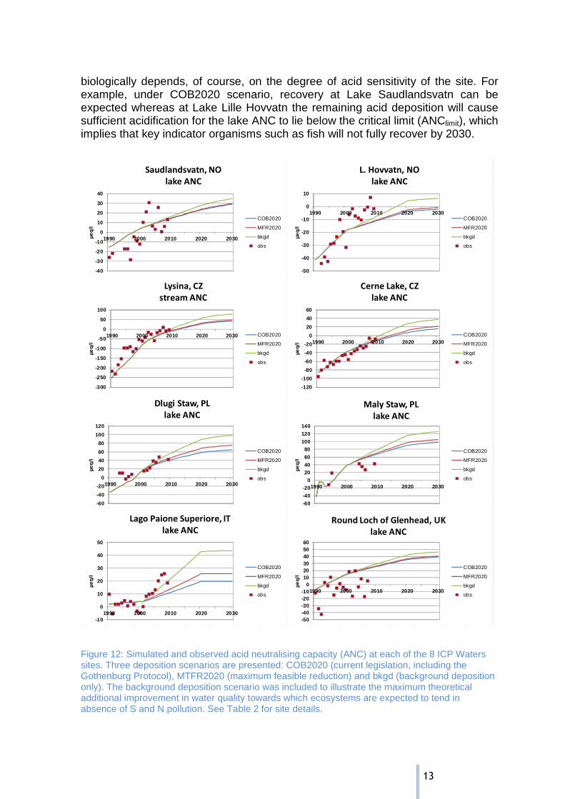
biologically depends, of course, on the degree of acid sensitivity of the site. For example, under COB2020 scenario, recovery at Lake Saudlandsvatn can be expected whereas at Lake Lille Hovvatn the remaining acid deposition will cause sufficient acidification for the lake ANC to lie below the critical limit (ANClimit), which implies that key indicator organisms such as fish will not fully recover by 2030.

-40

-30

-20

-10

0

10

20

30

40

1990 2000 2010 2020 2030µeq/

l

Saudlandsvatn, NO

lake ANC

COB2020

MFR2020

bkgd

obs

-50

-40

-30

-20

-10

0

10

1990 2000 2010 2020 2030

µeq/

l

L. Hovvatn, NO

lake ANC

COB2020

MFR2020

bkgd

obs

-300

-250

-200

-150

-100

-50

0

50

100

1990 2000 2010 2020 2030

µeq/

l

Lysina, CZ

stream ANC

COB2020

MFR2020

bkgd

obs

-120

-100

-80

-60

-40

-20

0

20

40

60

1990 2000 2010 2020 2030

µeq/

l

Cerne Lake, CZ

lake ANC

COB2020

MFR2020

bkgd

obs

-60

-40

-20

0

20

40

60

80

100

120

1990 2000 2010 2020 2030

µeq/

l

Dlugi Staw, PL

lake ANC

COB2020

MFR2020

bkgd

obs

-60-40-20

020406080

100120140

1990 2000 2010 2020 2030

µeq/

l

Maly Staw, PL

lake ANC

COB2020

MFR2020

bkgd

obs

-10

0

10

20

30

40

50

1990 2000 2010 2020 2030

µeq/

l

Lago Paione Superiore, IT

lake ANC

COB2020

MFR2020

bkgd

obs

-50-40-30-20-10

0102030405060

1990 2000 2010 2020 2030

µeq/

l

Round Loch of Glenhead, UK

lake ANC

COB2020

MFR2020

bkgd

obs

Figure 12: Simulated and observed acid neutralising capacity (ANC) at each of the 8 ICP Waters sites. Three deposition scenarios are presented: COB2020 (current legislation, including the Gothenburg Protocol), MTFR2020 (maximum feasible reduction) and bkgd (background deposition only). The background deposition scenario was included to illustrate the maximum theoretical additional improvement in water quality towards which ecosystems are expected to tend in absence of S and N pollution. See Table 2 for site details.

14

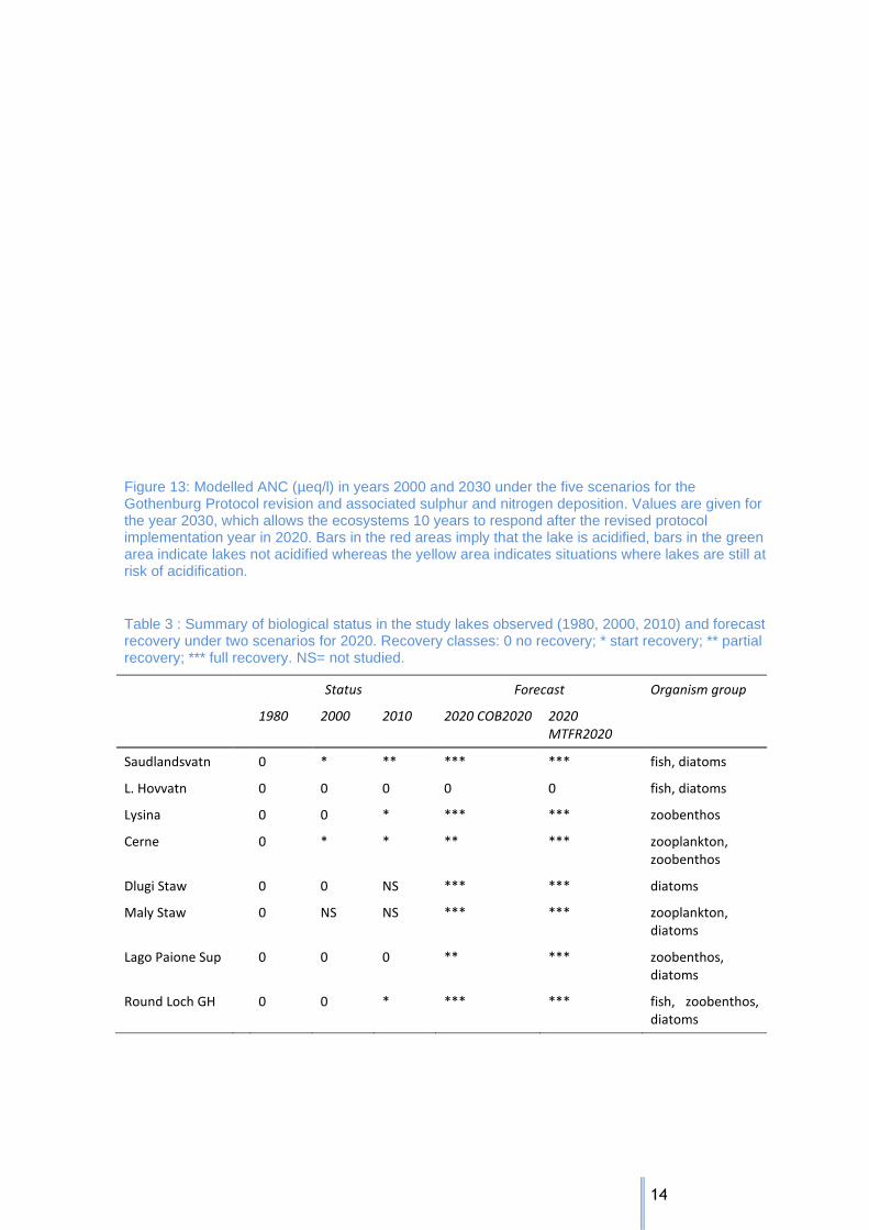
Figure 13: Modelled ANC (µeq/l) in years 2000 and 2030 under the five scenarios for the Gothenburg Protocol revision and associated sulphur and nitrogen deposition. Values are given for the year 2030, which allows the ecosystems 10 years to respond after the revised protocol implementation year in 2020. Bars in the red areas imply that the lake is acidified, bars in the green area indicate lakes not acidified whereas the yellow area indicates situations where lakes are still at risk of acidification.

Table 3 : Summary of biological status in the study lakes observed (1980, 2000, 2010) and forecast recovery under two scenarios for 2020. Recovery classes: 0 no recovery; * start recovery; ** partial recovery; *** full recovery. NS= not studied.

Status Forecast Organism group

1980 2000 2010 2020 COB2020 2020

MTFR2020

Saudlandsvatn 0 * ** *** *** fish, diatoms

L. Hovvatn 0 0 0 0 0 fish, diatoms

Lysina 0 0 * *** *** zoobenthos

Cerne 0 * * ** *** zooplankton,

zoobenthos

Dlugi Staw 0 0 NS *** *** diatoms

Maly Staw 0 NS NS *** *** zooplankton,

diatoms

Lago Paione Sup 0 0 0 ** *** zoobenthos,

diatoms

Round Loch GH 0 0 * *** *** fish, zoobenthos,

diatoms

15

3.3 ICP INTEGRATED MONITORING: EUTROPHICATION AND ACIDIFICATION OF FORESTED CATCHMENTS

3.3.1 ASSESSMENTS OF CRITICAL LOADS AT ICP IM SITES Critical loads for acidification CLA, calculated critical load of nutrient nitrogen CLnutN and empirical critical loads for nutrient nitrogen CLempN were evaluated at ICP Integrated Monitoring (IM) sites. Exceedance of critical loads were estimated for the NAT2000, COB2020, Low*2020, MID2020, High*2020 and MTFR2020 scenarios. Furthermore, the relationships between present exceedances of critical loads of acidification and eutrophication for terrestrial and aquatic ecosystems (using NAT2000 deposition scenario) and empirical surface water chemistry results were studied. The collected empirical data of the ICP IM was used for testing/validating the key concepts in the critical load calculations and for assessing the confidence in the regional scale critical loads mapping approach used in the integrated assessment modelling. Critical loads for acidification (CLA) of aquatic ecosystems were calculated for 17 IM sites, for which observations of runoff volume and water chemistry were available. The Steady-State Water Chemistry (SSWC) algorithm embedded in the FAB model was used (Henriksen and Posch, 2001, UBA, 2004 updated). Critical loads for eutrophication of terrestrial ecosystems were evaluated by two different methods: CLnutN are computed with the mass balance model for critical load of nutrient nitrogen, whereas CLempN are based on empirical critical loads for nutrient nitrogen. Both approaches are described in the manual for modelling and mapping critical loads and levels (UBA 2004 updated). Mass balance critical loads for nutrient nitrogen CLnutN were calculated with a nitrogen budget equation for the same 17 IM sites for which observations of runoff volume were available, with the addition of information for one site. Details of the calculations were carried out according to Holmberg et al. (2009, 2012). The empirical critical loads of nitrogen CLempN were compiled for another 24 sites in addition to those mentioned above. This analysis was based on reported critical loads of nutrient nitrogen from extensive empirical studies on the response of terrestrial ecosystems to nitrogen deposition (Bobbink and Hettelingh 2011). Calculations with the High*2020 and MTFR2020 scenarios reduced the average exceedance of CLA for aquatic ecosystems (Table 4) and increased the number of ICP IM sites protected from acidification from 11 under NAT2020 to 12. However, due to the sensitivity of the sites, even the MTFR2020 scenario would not protect all the sites. Regarding the critical loads for eutrophication for terrestrial ecosystems (CLnutN and CLempN) only the High*2020 and MTFR2020 scenarios would significantly reduce the average exceedance of critical loads and protect most of the plots in the ICP IM sites (Table 4 and Figure 14). With the MTFR2020 scenario, the total N deposition is lower than that of the High*2020 scenario only at 80% of the IM sites in the CLempN analysis.

16

Table 4: Average exceedance of critical loads for acidification CLA and eutrophication CLnutN and CLempN at ICP IM sites according to the Gothenburg Protocol scenarios.

Average exceedance

Nr of sites or plots in calculations

NAT2000 COB2020 Low*2020 MID2020 High*2020 MTFR2020

CLA

(eq ha-1yr-1)

994

463

338

360

322

331

17 sites

CLnutN .

(eq ha-1yr-1) (kg ha-1yr-1)

608

8.5

354

5.0

269

3.8

270

3.8

260

3.6

230

3.2

18 sites

CLempN

(eq ha-1yr-1)

(kg ha-1yr-1)

421

5.9

193

2.7

121

1.7

107

1.5

57

0.8

50

0.7

83 plots on 37 sites

6752 47 47

31 29

1631 36 36

52 54

0

20

40

60

80

100

NAT2000 COB2020 Low*2020 MID2020 High*2020 MFR2020

Nr of plots not protected Nr of plots protected

Figure 14: Number of plots in ICP IM sites that are protected/not protected from eutrophication (according to calculations based on empirical critical loads) assuming different deposition scenarios.

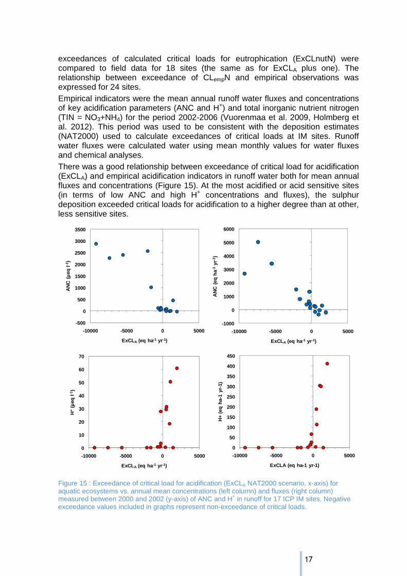
3.3.2 COMPARISON OF EXCEEDANCE OF CRITICAL LOADS WITH EMPI RICAL EFFECTS INDICATORS The collected empirical data of the ICP IM allows testing/validation of the regional scale critical loads mapping approach used under the LRTAP Convention and in particular, in integrated assessment modelling. Empirical observations and critical thresholds were compared for 17 to 24 IM sites, depending on availability of empirical monitoring data. The relationship between exceedances of critical loads for acidification (ExCLA) (using NAT2000 deposition scenario) and empirical observations was expressed for a selection of 17 sites, for which observations of runoff volume and runoff water chemistry were available. Correspondingly the

17

exceedances of calculated critical loads for eutrophication (ExCLnutN) were compared to field data for 18 sites (the same as for ExCLA plus one). The relationship between exceedance of CLempN and empirical observations was expressed for 24 sites. Empirical indicators were the mean annual runoff water fluxes and concentrations of key acidification parameters (ANC and H+) and total inorganic nutrient nitrogen (TIN = NO3+NH4) for the period 2002-2006 (Vuorenmaa et al. 2009, Holmberg et al. 2012). This period was used to be consistent with the deposition estimates (NAT2000) used to calculate exceedances of critical loads at IM sites. Runoff water fluxes were calculated water using mean monthly values for water fluxes and chemical analyses. There was a good relationship between exceedance of critical load for acidification (ExCLA) and empirical acidification indicators in runoff water both for mean annual fluxes and concentrations (Figure 15). At the most acidified or acid sensitive sites (in terms of low ANC and high H+ concentrations and fluxes), the sulphur deposition exceeded critical loads for acidification to a higher degree than at other, less sensitive sites.

-500

0

500

1000

1500

2000

2500

3000

3500

-10000 -5000 0 5000

AN

C (

µeq

l-1)

ExCLA (eq ha -1 yr -1)

-1000

0

1000

2000

3000

4000

5000

6000

-10000 -5000 0 5000

AN

C (

eq h

a-1

yr-1

)

ExCLA (eq ha -1 yr -1)

0

50

100

150

200

250

300

350

400

450

-10000 -5000 0 5000

H+

(eq

ha-1

yr-

1)

ExCLA (eq ha-1 yr-1)

0

10

20

30

40

50

60

70

-10000 -5000 0 5000

H+

(µeq

l-1

)

ExCLA (eq ha -1 yr -1)

Figure 15 : Exceedance of critical load for acidification (ExCLA NAT2000 scenario, x-axis) for aquatic ecosystems vs. annual mean concentrations (left column) and fluxes (right column) measured between 2000 and 2002 (y-axis) of ANC and H+ in runoff for 17 ICP IM sites. Negative exceedance values included in graphs represent non-exceedance of critical loads.

18

Regarding nitrogen enrichment (eutrophication) of terrestrial ecosystems, there is also evidence on the link between exceedance of critical loads of nutrient nitrogen and nitrogen leaching (Figure 16). At the sites in which mass balance nutrient nitrogen (CLnutN) and empirical critical load of nutrient nitrogen for terrestrial ecosystems (CLempN) were exceeded higher nitrate concentrations and fluxes in runoff were observed. These observations give evidence on links between modelled critical thresholds and empirical results for acidification parameters and nutrient nitrogen. They also increase confidence in the regional scale critical loads mapping approach

.

0

20

40

60

80

100

120

-2000 -1000 0 1000 2000

TIN

(µeq

l-1

)

0

20

40

60

80

100

120

140

-2000 -1000 0 1000 2000

TIN

(eq

ha-1

yr-

1)

ExCLnutN (eq ha-1 yr-1)

0

20

40

60

80

100

120

-500 0 500 1000

TIN

(µeq

l-1

)

0

20

40

60

80

100

120

140

-500 0 500 1000

TIN

(eq

ha-1

yr-

1)

ExCLempN (eq ha-1 yr-1) Figure 16: Exceedance of critical load for mass balance nutrient nitrogen (ExCLnutN, x-axis) vs. mean annual fluxes (left down) and concentrations (left upper) (2000-2002) (y-axis) of TIN (NO3+NH4) in runoff for 16 to 18 ICP IM sites, and exceedance of empirical values of critical load for nutrient nitrogen (ExCLempN, eq ha-1 yr-1x-axis) vs. mean annual fluxes (right down) and concentrations (right up) (2000-2002) (y-axis) of TIN (NO3+NH4) in runoff for 16-24 ICP IM sites. Exceedance values were calculated using the NAT2000 deposition scenario. Negative exceedance values included in graphs represent non-exceedance of critical loads. The sites with a significant input of N from sources other than deposition are denoted with a lighter green circle.

19

3.4 ICP MODELLING AND MAPPING: EUTROPHICATION, ACIDIFICATION , BIODIVERSITY CHANGES AT EUROPEAN SCALE

3.4.1 ACCUMULATED AVERAGE EXCEEDANCES AND AREAS AT RISK OF ACIDIFICATION AND EUTROPHICATION The Coordination Centre for Effects (CCE) of ICP Modelling and Mapping (ICP M&M) provides a European wide assessment of acidification and eutrophication through the calculation of several indicators: computed and empirical critical loads, target loads, their exceedances, losses of biodiversity, exceedances of critical limits... Computed critical loads are embedded in the GAINS model for integrated assessment modelling, whereas others are calculated outside GAINS. Together they are used in the Ensemble Assessment Impact to identify areas where impacts of atmospheric pollution are likely to occur (Hettelingh et al., 2011). Applied to the Gothenburg Protocol scenarios, these indicators show that whatever the chosen option, acidification and eutrophication will be reduced in 2020 compared to 2000 but impacts will remain over significant areas across Europe. Maps show that the intensity of critical loads exceedances decrease (less red on the maps) together with the areas impacted (more grey on the maps, Figure 17 and Figure 19). The decline in intensity and areas impacted can be used to rank the scenarios in the following (expected) order (from the least to the most favourable environmental conditions): COB2020, low*, MID, high*, MTFR. However, even with the MTFR scenario, 22 and 38% of the European and EU27 areas respectively will remain at risk of eutrophication while areas at risk of acidification will cover 1 and 3% of Europe and EU27 respectively (Table 5). Areas at risk for each UNECE country are given in Hettelingh et al. (2011). Table 5: Areas at risk of acidification and eutrophication in Europe according to the 5 scenarios tested for the revision of the Gothenburg Protocol. All % refer to the EU27 or European areas where calculated critical loads are exceeded.

% area at risk NAT2000 COB2020 Low* MID High* MTFR2 020

EU27 Eutrophication

Calculated

Empirical

75%

42%

59%

21%

50%

14%

48%

12%

44%

10%

38%

5%

Acidification 20% 6% 5% 4% 3% 3%

Europe Eutrophication

Calculated

Empirical

54%

25%

37%

11%

31%

7%

29%

6%

26%

5%

22%

3%

Acidification 12% 4% 3% 2% 2% 1%

Different from computed critical loads of N, which are based on models that simulate soil chemistry (UBA, 2004 updated), empirical critical loads have been established from field experiments in which reactive nitrogen is added in varying frequencies and quantities to establish ranges between a low and high exposure-thresholdat which vegetation changes occur. The fact that empirical critical loads

20

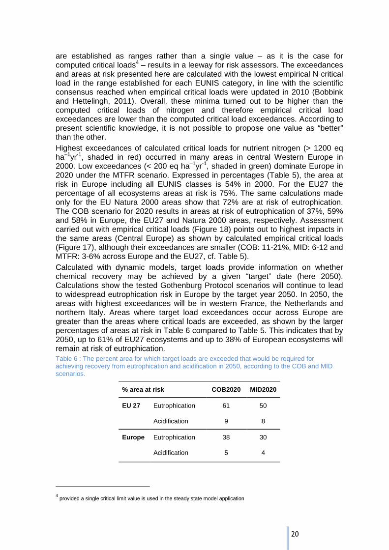
are established as ranges rather than a single value – as it is the case for computed critical loads4 – results in a leeway for risk assessors. The exceedances and areas at risk presented here are calculated with the lowest empirical N critical load in the range established for each EUNIS category, in line with the scientific consensus reached when empirical critical loads were updated in 2010 (Bobbink and Hettelingh, 2011). Overall, these minima turned out to be higher than the computed critical loads of nitrogen and therefore empirical critical load exceedances are lower than the computed critical load exceedances. According to present scientific knowledge, it is not possible to propose one value as “better” than the other. Highest exceedances of calculated critical loads for nutrient nitrogen (> 1200 eq ha–1yr-1, shaded in red) occurred in many areas in central Western Europe in 2000. Low exceedances (< 200 eq ha–1yr-1, shaded in green) dominate Europe in 2020 under the MTFR scenario. Expressed in percentages (Table 5), the area at risk in Europe including all EUNIS classes is 54% in 2000. For the EU27 the percentage of all ecosystems areas at risk is 75%. The same calculations made only for the EU Natura 2000 areas show that 72% are at risk of eutrophication. The COB scenario for 2020 results in areas at risk of eutrophication of 37%, 59% and 58% in Europe, the EU27 and Natura 2000 areas, respectively. Assessment carried out with empirical critical loads (Figure 18) points out to highest impacts in the same areas (Central Europe) as shown by calculated empirical critical loads (Figure 17), although their exceedances are smaller (COB: 11-21%, MID: 6-12 and MTFR: 3-6% across Europe and the EU27, cf. Table 5). Calculated with dynamic models, target loads provide information on whether chemical recovery may be achieved by a given “target” date (here 2050). Calculations show the tested Gothenburg Protocol scenarios will continue to lead to widespread eutrophication risk in Europe by the target year 2050. In 2050, the areas with highest exceedances will be in western France, the Netherlands and northern Italy. Areas where target load exceedances occur across Europe are greater than the areas where critical loads are exceeded, as shown by the larger percentages of areas at risk in Table 6 compared to Table 5. This indicates that by 2050, up to 61% of EU27 ecosystems and up to 38% of European ecosystems will remain at risk of eutrophication. Table 6 : The percent area for which target loads are exceeded that would be required for achieving recovery from eutrophication and acidification in 2050, according to the COB and MID scenarios.

% area at risk COB2020 MID2020

EU 27 Eutrophication 61 50

Acidification 9 8

Europe Eutrophication 38 30

Acidification 5 4

4 provided a single critical limit value is used in the steady state model application

21

The results for acidification are shown in Figure 19 and percentages of the areas at risk are given in Table 5. In 2000, the areas at risk of acidification are computed to cover 12% of the ecosystems in Europe, 20% in the EU27 and 23% of the EU-Natura 2000 areas. Peaks of exceedances (>1200 eq ha–1yr-1) in 2000 mostly occurred in Germany, Poland, the Netherlands and the United Kingdom. Current Legislation policies (scenario COB) reduces the occurrence of these peaks in 2020 to areas in Germany, Poland and the Netherlands, while low risk of acidification is seen to persist along an area from western France and the south of the British Isles to Poland as well as in southern parts of Scandinavian countries and in scattered areas further north and in Russia. Expressed in percentages the area at risk (Table 5) in Europe, the EU27 and Natura 2000 is calculated to be 4%, 6% and 7%, respectively. As for eutrophication, targets loads calculation show that by 2050, recovery will not be possible over areas covering 5 and 9% of Europe and EU27 respectively under the COB2020 scenario even though critical loads exceedances will affect only 4-6% of European ecosystems areas.

eq ha-1a-1

no exceedance0 - 200200 - 400400 - 700700 - 1200> 1200

AAE nut N 2000

Depositions: EMEP MSC-WCCE

eq ha-1a-1

no exceedance0 - 200200 - 400400 - 700700 - 1200> 1200

AAE nut N CLE 2020

Depositions: EMEP MSC-WCCE

eq ha-1a-1

no exceedance0 - 200200 - 400400 - 700700 - 1200> 1200

AAE nut N Low-star 2020

Depositions: EMEP MSC-WCCE

eq ha-1a-1

no exceedance0 - 200200 - 400400 - 700700 - 1200> 1200

AAE nut N MID 2020

Depositions: EMEP MSC-WCCE

eq ha-1a-1

no exceedance0 - 200200 - 400400 - 700700 - 1200> 1200

AAE nut N High-star 2020

Depositions: EMEP MSC-WCCE

eq ha-1a-1

no exceedance0 - 200200 - 400400 - 700700 - 1200> 1200

AAE nut N MFR 2020

Depositions: EMEP MSC-WCCE

COB20202000 Low* 2020

High*2020 MTFR2020MID 2020

Figure 17: Average Accumulated Exceedance (AAE) of computed critical loads for eutrophication in 2000 and 2020 under the COB, low*, MID, high* and MTFR scenarios. The areas with peaks of exceedances in 2000 (red shading) are markedly decreased in 2020. However, area at risk of nutrient nitrogen (size of shades indicates relative area coverage) remain widely distributed over Europe in 2020, even under MTFR.

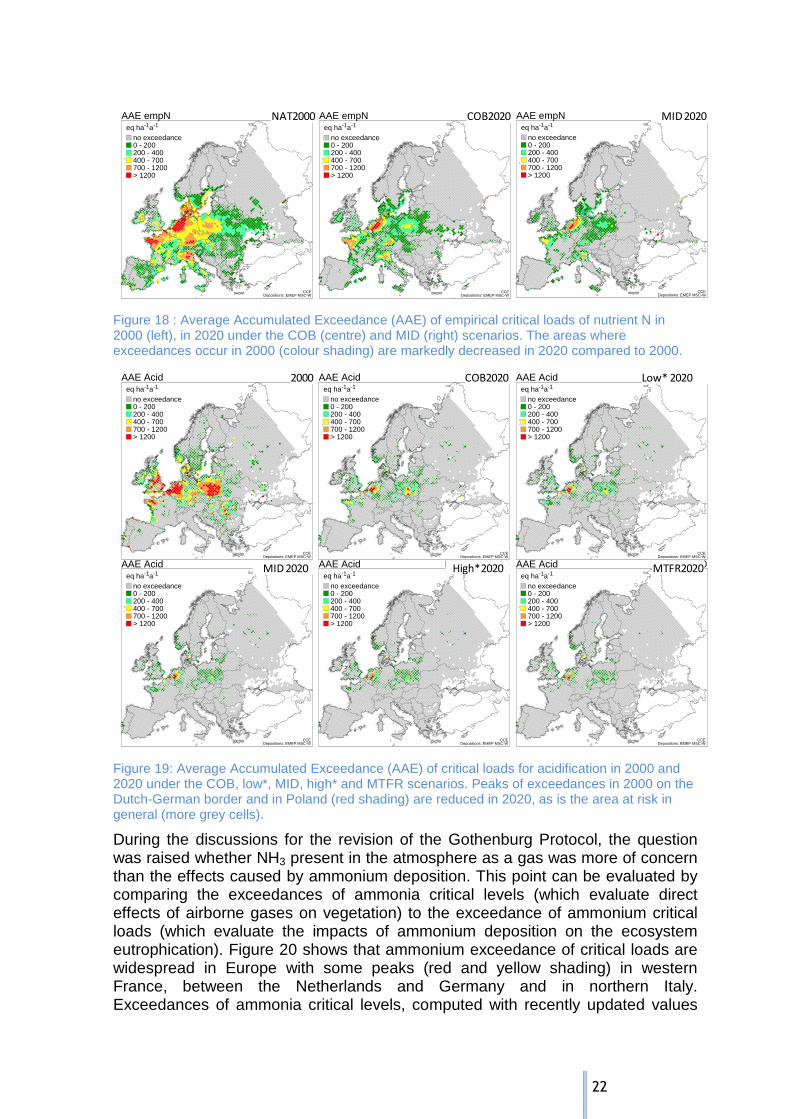
22

eq ha-1a-1

no exceedance0 - 200200 - 400400 - 700700 - 1200> 1200

AAE empN 2000

Depositions: EMEP MSC-WCCE

eq ha-1a-1

no exceedance0 - 200200 - 400400 - 700700 - 1200> 1200

AAE empN CLE 2020

Depositions: EMEP MSC-WCCE

AAE empN MID 2020 AAE empN High-star 2020

COB2020NAT2000eq ha-1a-1

no exceedance0 - 200200 - 400400 - 700700 - 1200> 1200

AAE empN MID 2020

Depositions: EMEP MSC-WCCE

MID 2020

Figure 18 : Average Accumulated Exceedance (AAE) of empirical critical loads of nutrient N in 2000 (left), in 2020 under the COB (centre) and MID (right) scenarios. The areas where exceedances occur in 2000 (colour shading) are markedly decreased in 2020 compared to 2000.

eq ha-1a-1

no exceedance0 - 200200 - 400400 - 700700 - 1200> 1200

AAE Acid 2000

Depositions: EMEP MSC-WCCE

eq ha-1a-1

no exceedance0 - 200200 - 400400 - 700700 - 1200> 1200

AAE Acid CLE 2020

Depositions: EMEP MSC-WCCE

eq ha-1a-1

no exceedance0 - 200200 - 400400 - 700700 - 1200> 1200

AAE Acid Low-star 2020

Depositions: EMEP MSC-WCCE

eq ha-1a-1

no exceedance0 - 200200 - 400400 - 700700 - 1200> 1200

AAE Acid MID 2020

Depositions: EMEP MSC-WCCE

eq ha-1a-1

no exceedance0 - 200200 - 400400 - 700700 - 1200> 1200

AAE Acid High-star 2020

Depositions: EMEP MSC-WCCE

eq ha-1a-1

no exceedance0 - 200200 - 400400 - 700700 - 1200> 1200

AAE Acid MFR 2020

Depositions: EMEP MSC-WCCE

COB20202000 Low* 2020

High*2020 MTFR2020MID 2020

Figure 19: Average Accumulated Exceedance (AAE) of critical loads for acidification in 2000 and 2020 under the COB, low*, MID, high* and MTFR scenarios. Peaks of exceedances in 2000 on the Dutch-German border and in Poland (red shading) are reduced in 2020, as is the area at risk in general (more grey cells).

During the discussions for the revision of the Gothenburg Protocol, the question was raised whether NH3 present in the atmosphere as a gas was more of concern than the effects caused by ammonium deposition. This point can be evaluated by comparing the exceedances of ammonia critical levels (which evaluate direct effects of airborne gases on vegetation) to the exceedance of ammonium critical loads (which evaluate the impacts of ammonium deposition on the ecosystem eutrophication). Figure 20 shows that ammonium exceedance of critical loads are widespread in Europe with some peaks (red and yellow shading) in western France, between the Netherlands and Germany and in northern Italy. Exceedances of ammonia critical levels, computed with recently updated values

23

(Cape et al., 2009), occur in the same areas. This implies that ammonia contributes to the risk of eutrophication across Europe and where this risk is highest, it is associated to a risk of exceeding concentrations of ammonia above which vegetation may be damaged. The comparison of the COB2020 and MID2020 scenarios shows that exceedances of ammonium critical loads and ammonia critical levels decrease in a similar way (Figure 20).

ugNH3m-3

no exceedance<44.0 - 5.0> 5.0

Exc. of [NH3] CLe CLE 2020

Conc-data: EMEP/MSC-WCCE

eq ha-1a-1

no exceedance<200200 - 400400 - 600600 - 800> 800

Exc. of CLnutN by NH4 CLE 2020

Dep-data: EMEP/MSC-WCCE

ugNH3m-3

no exceedance<44.0 - 5.0> 5.0

Exc. of [NH3] CLe MID 2020

Conc-data: EMEP/MSC-WCCE

eq ha-1a-1

no exceedance<200200 - 400400 - 600600 - 800> 800

Exc. of CLnutN by NH4 MID 2020

Dep-data: EMEP/MSC-WCCE

Exc. [NH3] critical levels COB2020

Exc. [NH3] critical levels MID 2020

Exc. [NH3] critical levels COB2020 Exc. CLd Nut N by NH4 COB2020

Exc. CLd Nut N by NH4 MID 2020

µg NH3 m-3

µg NH3 m-3

eq ha-1yr-1

eq ha-1yr-1

no exceedance<44.0 – 5.0>5.0

no exceedance<44.0 – 5.0>5.0

no exceedance< 200200 - 400400 - 600600 - 800> 800

no exceedance< 200200 - 400400 - 600600 - 800> 800

Figure 20 : Areas at risk of the exceedance of the critical level for ammonia in 2020 under the COB (top left) and MID (bottom left) scenarios in comparison to the areas at risk of the exceedance by the deposition of ammonium of the critical load of nutrient N under the COB (top right) and MID scenarios.

3.4.2 RISKS OF SIGNIFICANT CHANGE IN PLANT BIODIVERSITY The analysis of the change in biodiversity consists in a numerical estimation of the effects of scenario-specific nitrogen deposition in 2000 and 2020 (i) on the species richness of (semi-)natural grasslands (EUNIS class E), (ii) on the species richness of arctic and (sub-)alpine scrub habitats (EUNIS class F2) and (iii) on the Sorensen’s similarity index of the understorey vegetation of coniferous boreal woodlands (EUNIS class G3 A-C). Thus “change in biodiversity” is used as a common name for any of these indicators.

24

This analysis is based on dose-response curves (Bobbink, 2008; Bobbink and Hettelingh, 2011) that have been applied to these three EUNIS classes in Europe (Hettelingh et al., 2008), using the European harmonized land cover map (Slootweg et al., 2009). Here biodiversity change is considered significant if the indicator changed by more than 5% relative to its value in a control area (where the dose response curve has been established). The choice of 5% as a threshold percentage for identifying a “significant” change of biodiversity was arbitrary. It takes stock of widely applied statistical conventions regarding the analysis and representation of phenomena for which confidence levels need to be established. The indicator thus derived is used only to evaluate the relative changes caused by differences between deposition scenarios. Uncertainties associated with its calculation prevent from using its absolute values. These uncertainties are discussed in Hettelingh et al (2011). Results are shown on Figure 21 and in Table 7. The area at risk of a significant change in biodiversity evolves from covering many countries in 2000 to concerning predominantly northern Italy and the bordering area between Germany and the Netherlands in 2020 under MTFR.

change> 5%

Change in biodiversity (E,F2,G3) 2000

Dep-data: EMEPCCE

change> 5%

Change in biodiversity (E,F2,G3) CLE 2020

Dep-data: EMEPCCE

change> 5%

Change in biodiversity (E,F2,G3) Low* 2020

Dep-data: EMEPCCE

change> 5%

Change in biodiversity (E,F2,G3) MID 2020

Dep-data: EMEPCCE

change> 5%

Change in biodiversity (E,F2,G3) High* 2020

Dep-data: EMEPCCE

change> 5%

Change in biodiversity (E,F2,G3) MFR 2020

Dep-data: EMEPCCE

Figure 21: The location of natural areas (covering about half, i.e. about 2 million km2, of the European natural area characterised by the EUNIS classification) where the computed change of biodiversity is higher than 5% (red shading) in 2000 (top-left) and in 2020 under the COB (top-centre), low* (top-right), MID (bottom-left), high* (bottom-centre) and MTFR (bottom-right) scenarios.

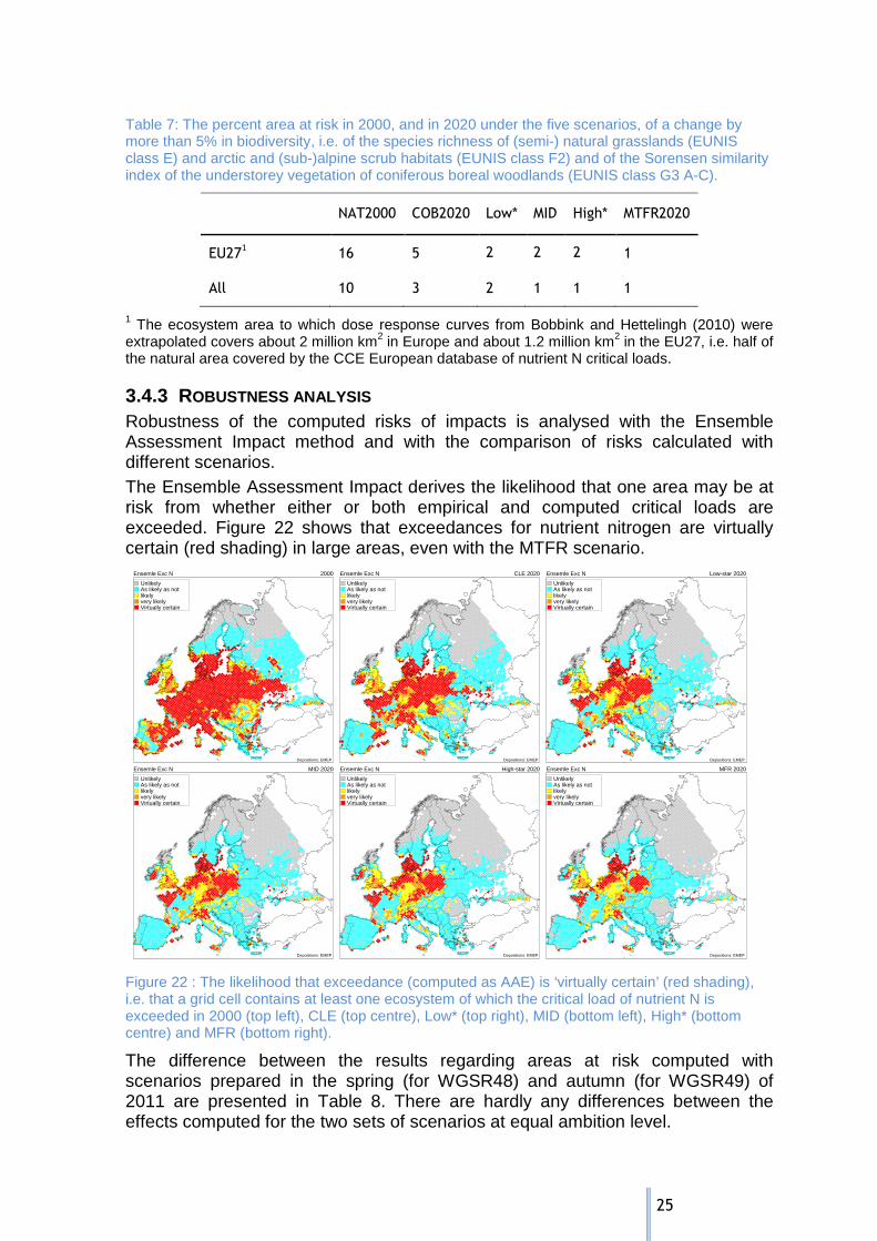
25

Table 7: The percent area at risk in 2000, and in 2020 under the five scenarios, of a change by more than 5% in biodiversity, i.e. of the species richness of (semi-) natural grasslands (EUNIS class E) and arctic and (sub-)alpine scrub habitats (EUNIS class F2) and of the Sorensen similarity index of the understorey vegetation of coniferous boreal woodlands (EUNIS class G3 A-C).

NAT2000 COB2020 Low* MID High* MTFR2020

EU271 16 5 2 2 2 1

All 10 3 2 1 1 1

1 The ecosystem area to which dose response curves from Bobbink and Hettelingh (2010) were extrapolated covers about 2 million km2 in Europe and about 1.2 million km2 in the EU27, i.e. half of the natural area covered by the CCE European database of nutrient N critical loads.

3.4.3 ROBUSTNESS ANALYSIS Robustness of the computed risks of impacts is analysed with the Ensemble Assessment Impact method and with the comparison of risks calculated with different scenarios. The Ensemble Assessment Impact derives the likelihood that one area may be at risk from whether either or both empirical and computed critical loads are exceeded. Figure 22 shows that exceedances for nutrient nitrogen are virtually certain (red shading) in large areas, even with the MTFR scenario.

UnlikelyAs likely as notlikelyvery likelyVirtually certain

Ensemle Exc N 2000

Depositions: EMEP

UnlikelyAs likely as notlikelyvery likelyVirtually certain

Ensemle Exc N CLE 2020

Depositions: EMEP

UnlikelyAs likely as notlikelyvery likelyVirtually certain

Ensemle Exc N Low-star 2020

Depositions: EMEP

UnlikelyAs likely as notlikelyvery likelyVirtually certain

Ensemle Exc N MID 2020

Depositions: EMEP

UnlikelyAs likely as notlikelyvery likelyVirtually certain

Ensemle Exc N High-star 2020

Depositions: EMEP

UnlikelyAs likely as notlikelyvery likelyVirtually certain

Ensemle Exc N MFR 2020

Depositions: EMEP

Figure 22 : The likelihood that exceedance (computed as AAE) is ‘virtually certain’ (red shading), i.e. that a grid cell contains at least one ecosystem of which the critical load of nutrient N is exceeded in 2000 (top left), CLE (top centre), Low* (top right), MID (bottom left), High* (bottom centre) and MFR (bottom right).

The difference between the results regarding areas at risk computed with scenarios prepared in the spring (for WGSR48) and autumn (for WGSR49) of 2011 are presented in Table 8. There are hardly any differences between the effects computed for the two sets of scenarios at equal ambition level.

26

Table 8 : Percentages of the area at risk of acidification and eutrophication as computed in support of policy processes in the 48th session of the Working Group on Strategies and Review (WGSR48) in the spring of 2011, in comparison to those submitted to the WGSR49.

% Area at Risk

Eutrophication Acidification

Scenario

48th WGSR 49th WGSR 48th WGSR 49th WGSR

Europe EU27 Europe EU27 Europe EU27 Europe EU27

2000 - - 54 75 - - 12 20

COB 37 58 37 59 3 6 4 6

Low* 30 48 31 50 3 5 3 5

MID 28 46 29 48 2 4 2 4

High* 25 42 26 38 2 3 2 3

MTFR 21 36 22 38 1 3 1 3

The coherence observed between the various indicators and when using different sets of scenario implies that conclusions drawn from the indicators proposed here are robust.

3.5 ICP VEGETATION: OZONE IMPACTS ON VEGETATION AND CROPS

3.5.1 BACKGROUND The indicators used in the Gothenburg Protocol to protect crops, trees and (semi-) natural vegetation from adverse impacts of ozone are based on the concentration metric, AOT40. Currently, the SOMO35 indicator for health is used for optimisation in the GAINS model and both the SOMO35 and the AOT40 for trees (accumulated from April to September) are included for reporting impacts of ozone. However, scientific research has developed significantly in the last decade and the accumulated ozone flux via leaf pores (stomatal flux) is now considered to provide a more biologically sound method for describing observed effects than the AOT40. It is calculated from the effects of climate (temperature, humidity, light), ozone, soil moisture availability and plant growth stage on the extent of opening of the stomatal pores through which ozone enters the plant. Led by the ICP Vegetation, several workshops held under the Working Group on Effects have developed ozone flux modelling methods and indicators for use in integrated assessment modelling. In 2010, the accumulated ozone flux via leaf pores was renamed as the Phytotoxic Ozone Dose above a threshold of Y, PODY (previously described as AFstY) and nine flux-based critical levels for vegetation have been established (ECE/EB.AIR/WG.1/2010/13; Harmens et al., 2010; Mills et al., 2011b, and update of Chapter 3 of the Manual on Methodologies and Criteria for Modelling and Mapping Critical Loads and Levels and Air Pollution Effects, Risks and Trends, UBA 2004 updated). An analysis of over 500 records of ozone damage to

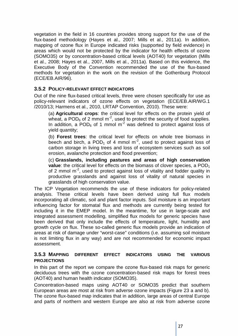
27

vegetation in the field in 16 countries provides strong support for the use of the flux-based methodology (Hayes et al., 2007; Mills et al., 2011a). In addition, mapping of ozone flux in Europe indicated risks (supported by field evidence) in areas which would not be protected by the indicator for health effects of ozone (SOMO35) or by concentration-based critical levels (AOT40) for vegetation (Mills et al., 2008; Hayes et al., 2007, Mills et al., 2011a). Based on this evidence, the Executive Body of the Convention recommended the use of the flux-based methods for vegetation in the work on the revision of the Gothenburg Protocol (ECE/EB.AIR/96).

3.5.2 POLICY-RELEVANT EFFECT INDICATORS Out of the nine flux-based critical levels, three were chosen specifically for use as policy-relevant indicators of ozone effects on vegetation (ECE/EB.AIR/WG.1 /2010/13; Harmens et al., 2010, LRTAP Convention, 2010). These were:

(a) Agricultural crops : the critical level for effects on the protein yield of wheat, a POD6 of 2 mmol m-2, used to protect the security of food supplies. In addition, a POD6 of 1 mmol m-2 was defined to protect against loss of yield quantity; (b) Forest trees : the critical level for effects on whole tree biomass in beech and birch, a POD1 of 4 mmol m-2, used to protect against loss of carbon storage in living trees and loss of ecosystem services such as soil erosion, avalanche protection and flood prevention; (c) Grasslands, including pastures and areas of high co nservation value : the critical level for effects on the biomass of clover species, a POD1 of 2 mmol m-2, used to protect against loss of vitality and fodder quality in productive grasslands and against loss of vitality of natural species in grasslands of high conservation value.

The ICP Vegetation recommends the use of these indicators for policy-related analysis. These critical levels have been derived using full flux models incorporating all climatic, soil and plant factor inputs. Soil moisture is an important influencing factor for stomatal flux and methods are currently being tested for including it in the EMEP model. In the meantime, for use in large-scale and integrated assessment modelling, simplified flux models for generic species have been derived that only include the effects of temperature, light, humidity and growth cycle on flux. These so-called generic flux models provide an indication of areas at risk of damage under “worst-case” conditions (i.e. assuming soil moisture is not limiting flux in any way) and are not recommended for economic impact assessment.

3.5.3 MAPPING DIFFERENT EFFECT INDICATORS USING THE VARIOU S PROJECTIONS In this part of the report we compare the ozone flux-based risk maps for generic deciduous trees with the ozone concentration-based risk maps for forest trees (AOT40) and human health indicator (SOMO35). Concentration-based maps using AOT40 or SOMO35 predict that southern European areas are most at risk from adverse ozone impacts (Figure 23 a and b). The ozone flux-based map indicates that in addition, large areas of central Europe and parts of northern and western Europe are also at risk from adverse ozone

28

impacts (Figure 23 c), risks that are not predicted using AOT40 or SOMO35. This can be explained by the favourable climatic conditions (e.g. high humidity) that enhance ozone stomatal flux in northern and western Europe at moderate ozone concentrations. On the other hand, lower humidity and higher temperature in southern Europe tend to reduce stomatal ozone flux at relatively high ozone concentrations. Thus in southern Europe, ozone concentrations are high but the flux to leaves is limited as the stomata are closed for long periods during hot hours of the day while in northern and western Europe, ozone concentrations are relatively low but its flux to leaves is hardly limited as the stomata remain open in humid conditions. The current data confirm previous results showing that policies aiming only at health effects would not protect vegetation in large areas of Europe (ECE/EB.AIR/96; Mills et al., 2008) and indicate that the additional risk to vegetation in parts of northern and western Europe remains of concern for future scenarios (Figure 24).

a: AOT40 b: SOMO 35 c: POD1 (beech)

Figure 23: The risk of adverse ozone impacts in 2000 a) on biomass production in forest as indicated by the concentration-based AOT40 for forest trees (the AOT40-based critical level is 5 ppm.h), b) on human health as indicated by SOMO35, c) on generic deciduous tree as calculated by the flux model (POD1). The maps were produced using the NAT 2000 projection.

a: COB2020 b: MID2020 c: MFR2020

Figure 24: The risk of adverse ozone impacts in 2020 on biomass production in forest using the generic deciduous tree flux model (POD1) for a) COB2020, b) MID2020, c) MTFR2020.

Comparison of ozone risk maps for vegetation applying the different scenarios and projections shows that despite the predicted reductions in both ozone concentrations and stomatal fluxes in the future, large areas in Europe will remain at risk from adverse impacts of ozone on vegetation, with areas at highest risk being predicted in parts of western, central and southern Europe (Figure 24). In Figure 25, the proportion of grid squares in each category illustrated on the maps

29

is shown for the four scenarios. Although for the 2020 scenarios there is a decrease in the proportion of grid squares in the highest categories, there remains a high proportion of grid squares in the middle to high categories (25 – 26% and 11 – 16% for a POD1 of 24 – 28 mmol m-2 and 28 – 32 mmol m-2 respectively), indicating a continuing risk of damage. Hence, additional measures to reduce the emissions of ozone precursors will be required to protect large areas in Europe from adverse impacts of ozone on vegetation in 2020.

Figure 25: Proportion of grid squares within specified categories of POD1 calculated using the generic forest flux model as calculated with the different datasets.

The ICP Vegetation also investigated the effects of ozone on wheat and tomato production (Mills and Harmens, 2011) using the scenarios available in 2010 (CIAM report 1/2010Figure 26 shows economic losses in million € per 50 x 50 km grid square for wheat. These are for the full wheat flux model, assuming irrigation is used whenever soil moisture is limiting. The critical level of 1 mmol m-2 for effects on yield (above which loss in yield is above 5% according to ICP Vegetation (2010)) is exceeded in 85% of Europe in 2000 representing 97% of the areas with wheat production (COB scenario, Figure 26 and Table 9), and total economic losses of €3.2 billion are predicted for EU27+CH+NO. Ozone critical level exceedance is only reduced to 82% of grid squares in 2020 when applying the COB projection, but the magnitude of the impact per grid square is decreased substantially reducing economic losses to €1.96 billion in 2020 (COB scenario). Ozone impacts were also quantified for tomato as an example of a horticultural crop commonly grown in southern Europe (as well as in other countries such as the Netherlands and Belgium). Using the flux-based method, economic losses of €1.02 billion representing 9.4% of production value were estimated for 2000 falling to €0.63 billion in 2020 (COB scenario, Table 9). The distribution of economic impacts on tomato is shown on Figure 27.

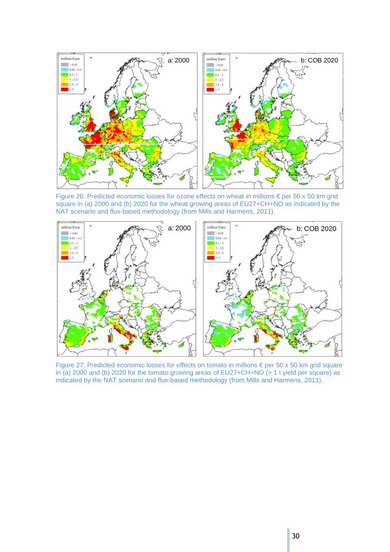
30

b: COB 2020a: 2000

Figure 26: Predicted economic losses for ozone effects on wheat in millions € per 50 x 50 km grid square in (a) 2000 and (b) 2020 for the wheat growing areas of EU27+CH+NO as indicated by the NAT scenario and flux-based methodology (from Mills and Harmens, 2011).

b: COB 2020a: 2000

Figure 27: Predicted economic losses for effects on tomato in millions € per 50 x 50 km grid square in (a) 2000 and (b) 2020 for the tomato growing areas of EU27+CH+NO (> 1 t yield per square) as indicated by the NAT scenario and flux-based methodology (from Mills and Harmens, 2011).

31

Table 9 : Predicted impacts of ozone pollution on wheat and tomato yield and economic value, together with critical level exceedance in EU27+Switzerland+Norway in 2000 and 2020 under the current legislation scenario (NAT scenario). Analysis was conducted on a 50 x 50 km EMEP grid square using crop values in 2000 and an ozone stomatal flux-based risk assessment (From Mills and Harmens, 2011).

Wheat Tomato

2000 2020 2000 2020

Total production, million t 133.53 17.68

Total economic value of wheat in 2000, billion Euro

15.87 6.85

Mean % yield loss per grid square 13.71 9.071 9.42 5.72

Total production loss, million t 26.89 16.45 2.64 1.62

Total economic value loss, billion Euro 3.20 1.96 1.02 0.63

Percentage of EMEP grid squares exceeding critical level 84.81 82.21 77.82 51.32

1based on all grid squares with wheat production, 2 based on grid squares with > 1 tonne of production

3.5.4 TEMPORAL TRENDS At the local scale there is evidence of higher ozone damage in years with higher ozone concentrations (e.g. 2003 and 2006) in regions in Europe where climatic conditions were conducive to high ozone fluxes (Hayes et al., 2007). However, there is no evidence of long-term trends related for example to the changing ozone profiles, i.e. lower peaks and higher background ozone concentrations (Royal Society, 2008).

3.5.5 OZONE IMPACTS IN A CHANGING CLIMATE BEYOND 2050 Apart from being a pollutant, ozone is also the third most important greenhouse gas, contributing to global warming. Hence, any measures to reduce the emissions of ozone will not only benefit air pollution but also climate change abatement policies. One main advantage of using the flux-based compared to the concentration-based approach for vegetation is that climate change factors (e.g. warming, relative humidity) affecting the opening of leaf pores and hence the uptake of ozone are included in calculating the ozone uptake by vegetation. Such factors are not included in the concentration-based indices. One important challenge for the future is to investigate whether dose-response relationships established under current climatic conditions still hold in a future changing climate. There is an urgent need to include the impacts of ozone on vegetation in global climate models using the flux based approach. Ozone pollution is likely to suppress the global carbon sink, leading to enhanced global warming (Sitch et al., 2007). Recent research has indicated that ozone concentrations within the ambient range might actually increase the opening of leaf pores, allowing increased ozone flux into the leaves and reducing drought tolerance in plants (Mills et al. 2009, Wilkinson & Davies, 2009, 2010). This may

32

lead to water loss from vegetation being far greater than currently included in global climate models.

3.6 ICP MATERIALS : CORROSION AND SOILING OF BUILDING MATERIALS INCLUDING CULTURAL HERITAGE ICP Materials has established indicators for corrosion of materials based on carbon steel, zinc and limestone reaction to air pollution. These indicators are expressed as corrosion in µm for a one-year exposure based on a material sample exposure for in situ monitoring or calculated from dose-response relationships for modelling work. Multi-pollutant relationships (UBA 2004 updated, chapter 4) are used in the present analysis. They include three scenario dependent parameters (SO2, HNO3 and PM10) as well as (temperature, relative humidity and hydrogen ion deposition due to precipitation (acid rain). In the present analysis, these last three parameters are considered scenario independent even if from a strict point of view they are scenario dependent. As they are not available from the scenarios provided by the TFIAM they have been derived from New et al (2002) for temperature, relative humidity and precipitation and by kriging of station data for pH in precipitation. Three criteria should be fulfilled for a material indicator: availability of (i) data on trends at ICP Materials test sites, (ii) reliable dose-response relationships, and (iii) acceptable and/or tolerable levels. The criteria (ii) and (iii) are necessary for calculating compliances of targets below. The criterion (i) is not necessary for this but is needed for validation of dose-response functions, which has not yet been made for soiling (Tidblad et al, 2010). These are all fulfilled for carbon steel, zinc and limestone but for soiling no single material fulfils all these criteria. Instead, a simplified synthesis of presently available data is used with PM10 as a material independent indicator for soiling based on the following general dose-response function:

∆R/R0 = 1 – exp(-k.t.PM10 )

where ∆R/R0 is the loss in reflectance compared to an unsoiled surface, k is a material constant equal to (2.2 ± 0.2) x 10-3 (year µg m-3)-1 based on data from limestone, painted steel and white plastic and t is the exposure time (Kucera et al, 2005). Targets for corrosion and soiling in 2020 and 2050 are given in Table 10. For 2050, corrosion of materials the relation is expressed as the percentage area where the corrosion rate of carbon steel, zinc or limestone exceeds the background corrosion rate by a factor of two. For soiling the relation is expressed as the area where the loss in reflectance of non-transparent materials compared to unsoiled surfaces exceeds 35 per cent in 20 years. The 35 per cent is a level indicating the need to clean the material. Table 11 shows overall compliances of these targets for the EUROPEAN region based on the dose-response relationships, on data from the scenarios and on the scenario-independent data. The last three entries (under the generic label “materials”) in the table give a combined result for materials based on all the individual compliance results. These combined results for materials are also illustrated by Figure 28.

33

Table 10: Targets for protecting materials of infrastructure and cultural heritage for 2020 and 2050 (ECE/EB.AIR/WG.1/2009/16 “Indicators and targets for air pollution effects”)

Indicator 2020 2050

Carbon steel corrosion < 20 µm year-1 < 16 µm year-1

Zinc corrosion < 1,1 µm year-1 < 0,9 µm year-1

Limestone corrosion < 8,0 µm year-1 < 6,5 µm year-1

Soiling measured as loss in reflectance compared to an unsoiled surface

< 35% after 10 years < 35% after 20 years

Table 11 : Compliances of targets of indicators for materials calculated from dose-response relationships for the whole EUROPEAN region in 2020.

2000 2020

Indicator Level(a)

NAT COB Low* MID High* MTFR

L: <16 µm 92.8% 99.5% 99.5% 99.8% 99.8% 99.9%

Carbon steel corrosion M: 16-20 µm 6.0% 0.5% 0.4% 0.2% 0.2% 0.1%

H: >20 µm 1.3% 0.0% 0.0% 0.0% 0.0% 0.0%

L: <0.9 µm 68.5% 89.0% 89.2% 91.3% 93.1% 94.1%

Zinc corrosion M: 0.9-1.1 µm 29.7% 10.9% 10.8% 8.7% 6.8% 5.9%

H: >1.1 µm 1.8% 0.0% 0.0% 0.0% 0.0% 0.0%

L: <6.5 µm 93.3% 99.4% 99.5% 99.6% 99.7% 99.8%

Limestone corrosion M: 6.5-8.0 µm 6.4% 0.6% 0.5% 0.4% 0.3% 0.2%

H: >8.0 µm 0.3% 0.0% 0.0% 0.0% 0.0% 0.0%

L: <10 µg m

-3 50.9% 87.8% 90.1% 92.3% 93.8% 95.2%

Soiling (PM10) M: 10-20 µg m

-3 48.0% 12.0% 9.8% 7.7% 6.2% 4.8%

H: >20 µg m

-3 1.1% 0.1% 0.1% 0.0% 0.0% 0.0%

L 50.4% 82.5% 84.2% 87.1% 89.3% 91.0%

“Materials” M 47.1% 17.3% 15.6% 12.8% 10.7% 9.0%

H 2.4% 0.2% 0.2% 0.0% 0.0% 0.0%

(a) L: 2050 targets met for all indicators M: intermediate cases not belonging to L or H H: 2020 target not met for at least one indicator

The 2050 targets are more difficult to meet than the 2020 targets, even though they are met at most locations (with the caveat of the urban area systematic difference as indicated in Table 11). Therefore when 2050 targets are met (L),

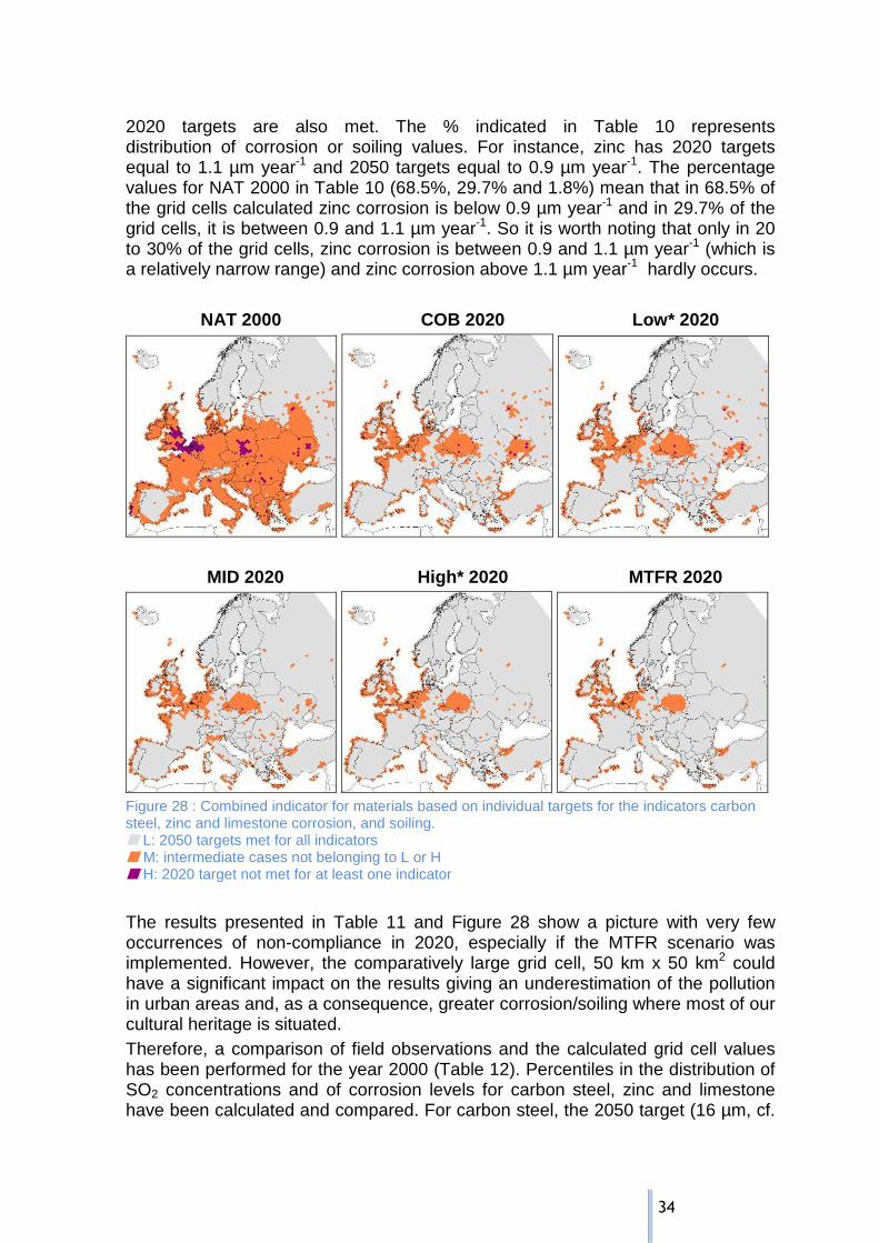
34

2020 targets are also met. The % indicated in Table 10 represents distribution of corrosion or soiling values. For instance, zinc has 2020 targets equal to 1.1 µm year-1 and 2050 targets equal to 0.9 µm year-1. The percentage values for NAT 2000 in Table 10 (68.5%, 29.7% and 1.8%) mean that in 68.5% of the grid cells calculated zinc corrosion is below 0.9 µm year-1 and in 29.7% of the grid cells, it is between 0.9 and 1.1 µm year-1. So it is worth noting that only in 20 to 30% of the grid cells, zinc corrosion is between 0.9 and 1.1 µm year-1 (which is a relatively narrow range) and zinc corrosion above 1.1 µm year-1 hardly occurs.

NAT 2000 COB 2020 Low* 2020

MID 2020 High* 2020 MTFR 2020

Figure 28 : Combined indicator for materials based on individual targets for the indicators carbon steel, zinc and limestone corrosion, and soiling. � L: 2050 targets met for all indicators � M: intermediate cases not belonging to L or H � H: 2020 target not met for at least one indicator

The results presented in Table 11 and Figure 28 show a picture with very few occurrences of non-compliance in 2020, especially if the MTFR scenario was implemented. However, the comparatively large grid cell, 50 km x 50 km2 could have a significant impact on the results giving an underestimation of the pollution in urban areas and, as a consequence, greater corrosion/soiling where most of our cultural heritage is situated. Therefore, a comparison of field observations and the calculated grid cell values has been performed for the year 2000 (Table 12). Percentiles in the distribution of SO2 concentrations and of corrosion levels for carbon steel, zinc and limestone have been calculated and compared. For carbon steel, the 2050 target (16 µm, cf.

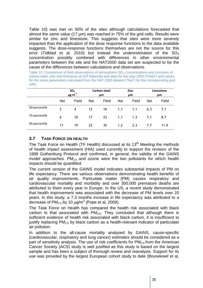
35

Table 10) was met on 50% of the sites although calculations forecasted that almost the same value (17 µm) was reached in 75% of the grid cells. Results were similar for zinc and limestone. This suggests that sites were more severely impacted than the application of the dose response functions to the data available suggests. The dose-response functions themselves are not the source for this error (Tidblad et al, 2010) but instead the underestimation of the SO2 concentration possibly combined with differences in other environmental parameters between the site and the NAT2000 data set are suspected to be the cause of the differences between calculations and observations. Table 12: Comparison of field observations of atmospheric SO2 concentrations and corrosion of carbon steel, zinc and limestone at ICP Materials test sites for the year 2000 (“Field”) and values for the same parameters calculated from the NAT 2000 dataset (“Nat”) for the corresponding grid cells.

SO2

µg m-3

Carbon steel

µm

Zinc

µm

Limestone

µm

Nat Field Nat Field Nat Field Nat Field

50-percentile 2 4 13 16 1.1 1.1 6.3 7.1

75-percentile 6 10 17 23 1.1 1.3 7.1 8.7

95-percentile 11 19 22 35 1.2 2.3 7.7 11.9

3.7 TASK FORCE ON HEALTH The Task Force on Health (TF Health) discussed at its 13th Meeting the methods of health impact assessment (HIA) used currently to support the revision of the 1999 Gothenburg Protocol and confirmed, in general, the validity of the GAINS model approaches. PM2.5 and ozone were the two pollutants for which health impacts should be quantified. The current version of the GAINS model indicates substantial impacts of PM on life expectancy. There are various observations demonstrating health benefits of air quality improvements. Particulate matter (PM) causes respiratory and cardiovascular mortality and morbidity and over 300,000 premature deaths are attributed to them every year in Europe. In the US, a recent study demonstrated that health improvement was associated with the decrease of PM levels over 20 years. In this study, a 7.3 months increase in life expectancy was attributed to a decrease of PM2.5 by 10 µg/m3 (Pope et al, 2009). The Task Force on Health has compared the health risk associated with black carbon to that associated with PM2.5. They concluded that although there is sufficient evidence of health risk associated with black carbon, it is insufficient to justify replacing PM2.5 by black carbon as a health-relevant indicator of particulate air pollution. In addition to the all-cause mortality analysed by GAINS, cause-specific (cardiovascular, respiratory and lung cancer) estimates should be considered as a part of sensitivity analysis. The use of risk coefficients for PM2.5 from the American Cancer Society (ACS) study is well justified as this study is based on the largest sample and has been a subject of thorough review and reanalysis. Support for its use was provided by the largest European cohort study to date (Brunekreef et al,

36

2009), which gives a risk estimate for all-cause mortality close to that from the ACS study. The TF Health has assessed effects on human health of black carbon as a component of PM2.5. It has found evidence of an association of black carbon (BC) variability with short-term changes of all cause and cardiovascular mortality, evidence of associations for all cause and cardiopulmonary mortality with long term average BC exposure, suggestive evidence that the effects of BC are (stronger) than those of PM10 or PM2.5 but insufficient evidence on a potential difference in the mechanisms of effects of BC in comparison to those of other potentially toxic component of PM2.5 and insufficient evidence to suggest any specific mechanism of effects of BC. Current calculations indicate that there are about 21 000 death per year in EU 25 accelerated by high concentrations (> 35 ppb or 70 µg.m-3) of ozone. Only small decrease of the impacts can be expected as a result of the current policies. The ozone HIA estimates should remain based on the SOMO35 indicator (annual sum of daily maximum mean eight-hour concentrations above 35 ppb), even though health impacts of ozone may occur at levels below 35 ppb. Recent studies suggest the impacts of long term exposure to ozone on respiratory symptoms and on mortality due to respiratory diseases. If further studies confirm these long term health effects, expansion of GAINS model to take into consideration impacts of long term average ozone exposures on respiratory mortality should be considered in the future. The dose response relationships still need to be confirmed.

4. DISCUSSION AND CONCLUSIONS

4.1 POLICY SUCCESSES MONITORED BY THE WORKING GROUP ON EFFECTS Measurements in the field remain the most effective and robust approach to monitor the effects of air policy on the environment. For example, the first and most direct consequence of pollutant emission reductions, the decrease of sulphur deposition, is now clearly recorded across several regions in Europe thanks to long–running observations at ICP Forests, ICP Waters and ICP Integrated Monitoring sites. Following the decrease of sulphur emissions to the atmosphere, the trends in several chemical indicators (such as pH, ANC) have been reversed: at many ICP Waters sites, pH and ANC are now increasing whereas they were decreasing in the 1980s and early 1990s. Biological recovery is still fragile but nevertheless on going in several parts of Europe (cf. for instance Figure 8 and Table 3 ). Responses of terrestrial ecosystems seems somewhat slower: Soil water pH at ICP Forests plots still exceeds critical limits for forests on half of the monitored plots (Fischer et al., 2010). Furthermore, a comparison between two surveys on more than 2000 level I plots showed that significant improvements in soil solid phase pH have been observed only on strongly acidified soils with pH below 4.0 between the end of the 1990s and the years 2004 to 2008 (De Vos and Cools, 2011). These improvements in ecosystems acidification status, whether they are clear in lakes and rivers or less obvious in forests, are the results of successful air pollution abatement policies across Europe.

37

Past policies have been less stringent for nitrogen emission reductions than for sulphur. This is also observed in the field: at 80% of ICP Forests level II sites, nitrogen depositions showed no significant changes between 1998 and 2007 (Fischer et al., 2010). Model results complement the information obtained via monitoring in the field. Modelling carried out by all ICPs clearly shows the important decrease of areas at risk of acidification, and, to a lesser extend, the decrease of areas at risk of eutrophication since 2000. Ozone affects both human health and vegetation growth. It is formed in the atmosphere in the presence of sunlight, NOx, and volatile organic compounds. Long term measurements indicate small decrease in peak ozone concentrations but rising background ozone concentrations. Recent modelling and monitoring work by ICP Vegetation has shown that ozone impacts were widespread in Europe and not mainly confined to southern European countries where concentrations are the highest. Impacts on human health are taken into account in integrated modelling, via the SOMO35 indicator in accordance with the work carried out by the TF Health. For PM, the TF Health has reported that improvement of air quality accounted for 15% of the overall increase in life expectancy in the US between 1980 and 2000 (Pope AC et al., 2009). These North American results are corroborated by a recent European study (Nawrot et al., 2011). Evidence is at the moment insufficient to evaluate the specific impact of black carbon on human health but the TF on Health recommends that PM2.5 concentrations remain the indicator for human health. It should not be replaced, at present, by black carbon concentrations.

4.2 SCIENTIFIC KNOWLEDGE : STATE OF THE ART The Working Group on Effects has developed and collated large amount of scientific and multidisciplinary knowledge related to the impact of air pollution on ecosystems, human health and materials. This work has been documented year after year in its ICPs and Task Force reports and summarised in the annual Working Group on Effects documentation. It has also been the basis of numerous publications in peer review scientific journals. The current assessment is the opportunity for an update and a focus of this knowledge. Thus, monitoring series presented and used here by ICP Forests, ICP Waters and ICP Integrated Monitoring include the most recent measurements. Indicators and modelling approaches from all ICPs presented here have mostly been developed (or improved) and validated under the Working Group on Effects and EMEP in the last 5 years. They are used for the first time to document and support policy decision for the revision of a protocol. Key scientific developments :

• Flux based indicators of ozone damage on vegetation and crops (Phytotoxic ozone dose, PODy) indicate that a large proportion of northern, western and central parts of Europe is at risk of ozone damage. The geographical extent of damage is underestimated by classical concentration based indicators (such AOT40). This conclusion is backed by evidence from field data collated by ICP Vegetation.

38

• Dynamic modelling allowed the assessment of recovery patterns and timing in aquatic and terrestrial ecosystems. It also made it possible to relate required deposition levels with chosen target year for recovery.

• Relative changes in biodiversity caused by nitrogen deposition have been quantified, from dose-response relationships applied to three types of ecosystems.

• An evaluation of material soiling and corrosion has been derived from dose-response relationships and set targets for the years 2020 and 2050.

• The coherence of monitoring data with modelled results, underlined again here by ICP Forests, ICP Waters, ICP Integrated Monitoring and ICP Vegetation, illustrates the robustness of the critical loads and levels methodology.

• Indicators recommended by the TF Health, the SOMO35 for ozone and relations between PM concentrations and year of life losses (YOLL), are currently taken into account in integrated assessment modelling. Present knowledge supports these two indicators and their use in the GAINS model so no new indicators have been considered in this report.

Informing future policy development Models run by the Working Group on Effects provide an insight into the potential impacts, or recovery that may be expected from the implementation of air pollution abatement policies. Two main results are derived from all WGE groups results:

• Improvements of the condition of the environment (in terms of acidification, eutrophication and ozone impact) are expected by 2020 even if regulations lead only to emission reductions considered in the least ambitious baseline scenario. In that scenario, little improvement of human health is expected as far as ozone effects are concerned.

• None of the scenarios considered would allow full recovery of ecosystems. Even with the MTFR scenario, the areas at risk of acidification in Europe would be greater than 2% and the most acidified sites of ICP Waters and ICP Integrated Monitoring would not recover. About 20% of the European area would still be at risk of eutrophication. Critical levels of ozone for vegetation will still be exceeded in large areas of Europe, including in >95% of the wheat growing areas. Also in about 5% of the European area the 2050 targets for materials would not be met.

In order to evaluate how policies will improve human health, the environment and damages to materials, the use of several indicators presented in this report has been proposed in the “Guidance Document VII on health and environmental improvements” of the revised Gothenburg Protocol. This document proposes to record and evaluate systematically policy-relevant indicators that measure the impact of air pollution abatement policies on the environment, on human health and materials. These indicators include the exceedance of critical loads, the loss of human years, the impact of ozone on crops etc.

39

4.3 ON-GOING EFFECT BASED SCIENTIFIC STUDIES TO SUPPORT THE LRTAP CONVENTION It is a fact of life that science is always in progress. In the framework of the Working Group on Effects, the main approaches that are currently being followed include:

• Continued monitoring: Long-term monitoring, field measurements and epidemiology studies are required tools to understand processes that control long term processes involved in air pollution and its impacts on ecosystems, materials and human health.

• Evaluation of nitrogen input and output fluxes showing how nitrogen is accumulating in watersheds. Under continuous inputs, it is expected that soil storage capacity fills up and that, as a consequence, nitrogen leaches to surface waters. Modelling catchment potential for continued N accumulation will help to forecast (and potentially to prevent) N leaching, potentially leading to nutrient imbalance in aquatic ecosystems.

• An evaluation of whether the modelled low values of base cations (calcium, potassium, magnesium, which are essential nutrients) in forest soils can be confirmed by field measurements and whether they may contribute to low base cations levels in connected freshwaters.

• Continued development of new endpoints and indicators to reflect societal concerns: Air pollution impacts on biodiversity and ecosystems services (such as water quality, carbon sequestration and recreational fisheries). Work in progress attempts to link such endpoints to critical loads and levels.

• Assessment of impacts of air pollution under changing climate: it will be necessary to:

o Evaluate whether the dose-response relationships established for ozone under present climate conditions still holds in a future climate.

o Model how climate change may slow down or setback recovery from acidification on a large scale.

• Evaluation of the impacts of ozone, including rising background concentrations on:

o Human health due to peak and chronic exposure. o Food security via impacts on crop yield. o Biodiversity and ecosystems services, such as carbon

sequestration. o Vegetation by inclusion in dynamic models. o Vegetation and crops in presence of nitrogen pollution.

• Evaluation of the impacts of particulate matter on materials of in urban pollution hotspots.

• Evaluation of the impacts of particulate matter on human health: in order to focus policies and to improve the effectiveness of their intervention, it is now necessary to consider the chemical and physical properties of particulate matter and their sources. In order to refine integrated

40

assessment modelling, it may be considered to calculate separately impacts of mortality due to cardio-pulmonary diseases and lung cancer instead of one estimates for all causes of death.

Pursuing these activities, the WGE groups have successfully gathered ong term series and data on ecosystems and health at country and European scale that are essential to provide:

• Answers to policy makers (via the WGSR and the Executive Body).

• Information on the efficiency of implemented policies.

• Forecasts on the efficiency of planned air pollution abatement policies.

4.4 OVERALL CONCLUSION The present analysis is the fruit of a robust collaboration between groups under EMEP and the Working Groups on Effects, responding to WGSR needs for information. It underlines the importance and the efficiency of the WGE interdisciplinary approach that combines monitoring, experimentation, and modelling to assess the sufficiency of air pollution abatement policies. The present analysis has been carried out in two steps: A first round of scenarios were analysed in 2010-2011. The second set of scenarios, illustrated here, was issued according to the WGSR48th recommendation. Only slight differences between both sets of scenarios were observed at European level. This supports the robustness of the LRTAP approach which involves atmospheric modelling, monitoring and modelling effects and integrated assessment modelling. This collaborative work leads to the following overall conclusion: Implemented reductions of air pollutant emissions lead to an improvement of the environment and human health. Yet, further efforts are required to reach conditions that would not damage ecosystems, crops, human health and materials.

41

5. BIBLIOGRAPHY Amann, M., Bertok, I., Cofala, J., Heyes, C., Klimont, Z., Rafaj, P., Schöpp, W.,

and Wagner, F. (2010). "Scope for further environmental improvements in 2020 beyond the baseline projections" Rep. No. CIAM Report 1/2010. IIASA, International institute for applied systems analysis, Laxenburg, Austria.

Amann M, Bertok I, Cofala J, Heyes C, Klimont Z, Rafaj P, Schöpp W, Wagner F, 2010. Scope for further environmental improvements in 2020 beyond the baseline projections, Background paper for the 47th Session of the Working Group on Strategies and Review of the Convention on Long-range Transboundary Air Pollution, Geneva, August 30 – September 3 2010, Centre for Integrated Assessment Modelling (CIAM), International Institute for Applied Systems Analysis (IIASA), CIAM Report 1/2010, http://gains.iiasa.ac.at/index.php/publications/policy-reports/gothenburg-protocol-revision.

Amann, M., Bertok, I., Borken-Kleefeld, J., Cofala, J., Heyes, C., Höglund-Isaksson, L., Klimont, Z., Rafaj, P., Schöpp, W., and Wagner, F. (2011a). "Cost-effective Emission Reductions to Improve Air Quality in Europe in 2020. Scenarios for the Negotiations on the Revision of the Gothenburg Protocol under the Convention on Long-range Transboundary Air Pollution." IIASA, International institute for applied systems analysis, Laxenburg, Austria.

Amann, M., Bertok, I., Borken-Kleefeld, J., Cofala, J., Heyes, C., Höglund-Isaksson, L., Klimont, Z., Rafaj, P., Schöpp, W., and Wagner, F. (2011b). "An Updated Set of Scenarios of Cost-effective Emission Reductions for the Revision of the Gothenburg Protocol." IIASA, International institute for applied systems analysis, Laxenburg, Austria.

Bobbink, R. (2008). The derivation of dose-response relationships between N load, N exceedance and plant species richness for EUNIS Habitat Classes. In "Critical load, dynamic modelling and impact assessment in Europe. CCE Status Report 2008" (J. P. Hettelingh, M. Posch and J. Slootweg, eds.), pp. 63-72. PBL Netherlands Environmental Assessment Agency, Bilthoven, Pays Bas.

Bobbink, R., and Hettelingh, J. P., eds. (2011). Review and revision of empirical critical loads and dose response relationships. Proceedings of an expert workshop, Noordwijkerhout, 23-24 June 2010. RIVM report 680359002. 244 pp.

Bonten L, Posch M, Reinds GJ (2009). Dynamic modelling of effects of deposition on carbon sequestration and nitrogen availability: VSD plus C and N dynamics (VSD+). In: Hettelingh JP, Posch M, Slootweg J (eds.) (2009) Progress in the modelling of critical thresholds, impacts to plant species diversity and ecosystem services in Europe: CCE Status Report 2009, Coordination Centre for Effects, www.pbl.nl/cce

Brunekreef, B., Beelen, R., Hoek, G., Schouten, L., Bausch-Goldbohm, S., Fischer, P., Armstrong, B., Hughes, E., Jerrett, M., and van den Brandt, P. (2009). "Effects of Long-Term Exposure to Traffic-Related Air Pollution on

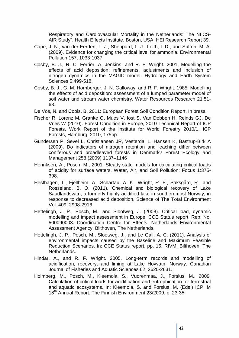
42

Respiratory and Cardiovascular Mortality in the Netherlands: The NLCS-AIR Study". Health Effects Institute, Boston, USA. HEI Research Report 39.

Cape, J. N., van der Eerden, L. J., Sheppard, L. J., Leith, I. D., and Sutton, M. A. (2009). Evidence for changing the critical level for ammonia. Environmental Pollution 157, 1033-1037.

Cosby, B. J., R. C. Ferrier, A. Jenkins, and R. F. Wright. 2001. Modelling the effects of acid deposition: refinements, adjustments and inclusion of nitrogen dynamics in the MAGIC model. Hydrology and Earth System Sciences 5:499-518.

Cosby, B. J., G. M. Hornberger, J. N. Galloway, and R. F. Wright. 1985. Modelling the effects of acid deposition: assessment of a lumped parameter model of soil water and stream water chemistry. Water Resources Research 21:51-63.

De Vos, N. and Cools, B. 2011: European Forest Soil Condition Report. In press. Fischer R, Lorenz M, Granke O, Mues V, Iost S, Van Dobben H, Reinds GJ, De

Vries W (2010). Forest Condition in Europe, 2010 Technical Report of ICP Forests. Work Report of the Institute for World Forestry 2010/1. ICP Forests, Hamburg, 2010, 175pp.

Gundersen P, Sevel L, Christiansen JR, Vesterdal L, Hansen K, Bastrup-Birk A (2009). Do indicators of nitrogen retention and leaching differ between coniferous and broadleaved forests in Denmark? Forest Ecology and Management 258 (2009) 1137–1146

Henriksen, A., Posch, M., 2001. Steady-state models for calculating critical loads of acidity for surface waters. Water, Air, and Soil Pollution: Focus 1:375-398.

Hesthagen, T., Fjellheim, A., Schartau, A. K., Wright, R. F., Saksgård, R., and Rosseland, B. O. (2011). Chemical and biological recovery of Lake Saudlandsvatn, a formerly highly acidified lake in southernmost Norway, in response to decreased acid deposition. Science of The Total Environment Vol. 409, 2908-2916.

Hettelingh, J. P., Posch, M., and Slootweg, J. (2008). Critical load, dynamic modelling and impact assessment in Europe. CCE Status report, Rep. No. 500090003. Coordination Centre for Effects, Netherlands Environmental Assessment Agency, Bilthoven, The Netherlands.

Hettelingh, J. P., Posch, M., Slootweg, J., and Le Gall, A. C. (2011). Analysis of environmental impacts caused by the Baseline and Maximum Feasible Reduction Scenarios. In: CCE Status report, pp. 15. RIVM, Bilthoven, The Netherlands.

Hindar, A., and R. F. Wright. 2005. Long-term records and modelling of acidification, recovery, and liming at Lake Hovvatn, Norway. Canadian Journal of Fisheries and Aquatic Sciences 62: 2620-2631.

Holmberg, M., Posch, M., Kleemola, S., Vuorenmaa, J., Forsius, M., 2009. Calculation of critical loads for acidification and eutrophication for terrestrial and aquatic ecosystems. In: Kleemola, S. and Forsius, M. (Eds.) ICP IM 18th Annual Report. The Finnish Environment 23/2009. p. 23-35.

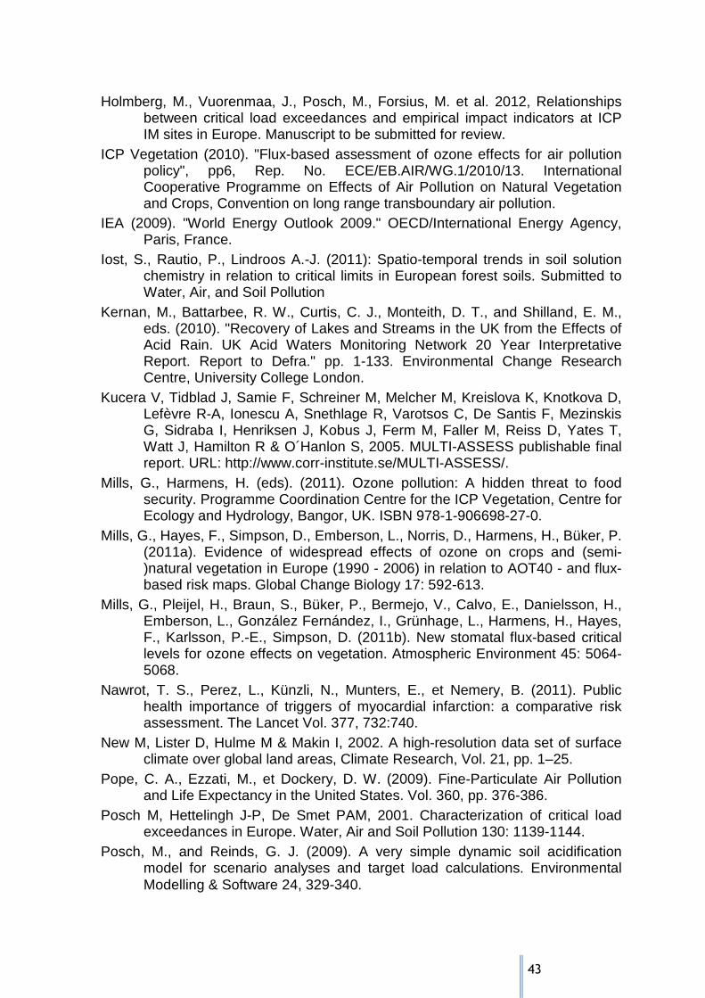
43

Holmberg, M., Vuorenmaa, J., Posch, M., Forsius, M. et al. 2012, Relationships between critical load exceedances and empirical impact indicators at ICP IM sites in Europe. Manuscript to be submitted for review.

ICP Vegetation (2010). "Flux-based assessment of ozone effects for air pollution policy", pp6, Rep. No. ECE/EB.AIR/WG.1/2010/13. International Cooperative Programme on Effects of Air Pollution on Natural Vegetation and Crops, Convention on long range transboundary air pollution.

IEA (2009). "World Energy Outlook 2009." OECD/International Energy Agency, Paris, France.

Iost, S., Rautio, P., Lindroos A.-J. (2011): Spatio-temporal trends in soil solution chemistry in relation to critical limits in European forest soils. Submitted to Water, Air, and Soil Pollution

Kernan, M., Battarbee, R. W., Curtis, C. J., Monteith, D. T., and Shilland, E. M., eds. (2010). "Recovery of Lakes and Streams in the UK from the Effects of Acid Rain. UK Acid Waters Monitoring Network 20 Year Interpretative Report. Report to Defra." pp. 1-133. Environmental Change Research Centre, University College London.

Kucera V, Tidblad J, Samie F, Schreiner M, Melcher M, Kreislova K, Knotkova D, Lefèvre R-A, Ionescu A, Snethlage R, Varotsos C, De Santis F, Mezinskis G, Sidraba I, Henriksen J, Kobus J, Ferm M, Faller M, Reiss D, Yates T, Watt J, Hamilton R & O´Hanlon S, 2005. MULTI-ASSESS publishable final report. URL: http://www.corr-institute.se/MULTI-ASSESS/.

Mills, G., Harmens, H. (eds). (2011). Ozone pollution: A hidden threat to food security. Programme Coordination Centre for the ICP Vegetation, Centre for Ecology and Hydrology, Bangor, UK. ISBN 978-1-906698-27-0.

Mills, G., Hayes, F., Simpson, D., Emberson, L., Norris, D., Harmens, H., Büker, P. (2011a). Evidence of widespread effects of ozone on crops and (semi-)natural vegetation in Europe (1990 - 2006) in relation to AOT40 - and flux-based risk maps. Global Change Biology 17: 592-613.

Mills, G., Pleijel, H., Braun, S., Büker, P., Bermejo, V., Calvo, E., Danielsson, H., Emberson, L., González Fernández, I., Grünhage, L., Harmens, H., Hayes, F., Karlsson, P.-E., Simpson, D. (2011b). New stomatal flux-based critical levels for ozone effects on vegetation. Atmospheric Environment 45: 5064-5068.

Nawrot, T. S., Perez, L., Künzli, N., Munters, E., et Nemery, B. (2011). Public health importance of triggers of myocardial infarction: a comparative risk assessment. The Lancet Vol. 377, 732:740.

New M, Lister D, Hulme M & Makin I, 2002. A high-resolution data set of surface climate over global land areas, Climate Research, Vol. 21, pp. 1–25.

Pope, C. A., Ezzati, M., et Dockery, D. W. (2009). Fine-Particulate Air Pollution and Life Expectancy in the United States. Vol. 360, pp. 376-386.

Posch M, Hettelingh J-P, De Smet PAM, 2001. Characterization of critical load exceedances in Europe. Water, Air and Soil Pollution 130: 1139-1144.

Posch, M., and Reinds, G. J. (2009). A very simple dynamic soil acidification model for scenario analyses and target load calculations. Environmental Modelling & Software 24, 329-340.

44

Rogora, M. (2004). Acidification and recovery at mountain lakes in Central Alps assessed by the MAGIC model. J. Limnology 63, 133-142.

Rzychon, D., and Worsztynowicz, A. (2008). What affects nitrogen retention in Tatra Mountain lakes' catchments in Poland? Hydrology And Earth System Sciences 12, 415-424.

Rzychoń, D., Worsztynowicz, A., Samborska, K., and Ulańczyk, R. (2010). Use of the dynamic model MAGIC to reconstruction and predicting of long-term changes in lakes water chemistry in Karkonosze Mts. (in Polish). Opera Concortica. Krkonosske prace. 47. Suplementum 1, 35-47.

Schöpp W, Posch M, Mylona S, Johansson M, 2003. Long-term development of acid deposition (1880-2030) in sensitive freshwater regions in Europe. Hydrology and Earth System Sciences 7(4): 436-446

Seidling, W., Fisher, R., and Granke, O. (2008). Relationships between forest floor vegetation on ICP Forests monitoring plots in Europe and basic variables in soil and nitrogen deposition. International journal of environmental studies 65, 309-320.

Skjelkvåle, B. L., et de Wit, H., eds. (2008). "ICP Waters: 20 years of monitoring effects of long-range transboundary air pollution on surface waters in Europe and North America", pp. 1-55. International Cooperative Programme on assessment and monitoring of acidification of rivers and lakes, Convention on long-range transboundary air pollution, Oslo, Norway.

Slootweg, J. Posch, M., and Warrink, A. (2009). Status of the harmonised European land cover map. In "Progress in the modelling of critical thresholds, impacts to plant species diversity and ecosystem services in Europe: CCE status report 2009" (J. P. Hettelingh, M. Posch and J. Slootweg, eds.), pp. 31-34. Coordination Centre for Effects (CCE) Bilthoven, The Netherlands.

Tidblad J, De la Fuente D, Faller M and Kreislova K. ICP Materials Report No 64 Validity of dose-response functions for different climatic conditions, Swerea KIMAB, 2010

UBA 2004 updated. Manual on methodologies and criteria for modelling and mapping critical loads and levels and air pollution effects, risks and trends. UNECE Convention on Long-range Transboundary Air Pollution, Federal Environmental Agency (Umweltbundesamt), Berlin. http://www.icpmapping.org

Vuorenmaa, J., Kleemola, S., Forsius, M., 2009. Trend assessment of bulk deposition, throughfall and runoff water/soil water chemistry at ICP IM sites In: Kleemola, S. and Forsius, M. (Eds.) 18th Annual Report 2009. ICP Integrated Monitoring. The Finnish Environment 23/2009, pp. 36-63. Finnish Environment Institute, Helsinki.

Vrba, J., Kopacek, J., Fott, J., Kohout, L., Nedbalova, L., Prazakova, M., Soldan, T., and Schaumburg, J. (2003). Long-term studies (1871-2000) on acidification and recovery of lakes in the Bohemian Forest (central Europe). Science of the Total Environment 310, 73-85.

Wright, R. F., C. Alewell, J. Cullen, C. D. Evans, A. Marchetto, F. Moldan, A. Prechtel, and M. Rogora. 2001. Trends in nitrogen deposition and leaching

45

in acid-sensitive streams in Europe. Hydrology and Earth System Sciences 5:299-310.

Wright, R. F., T. Larssen, L. Camarero, B. J. Cosby, R. C. Ferrier, R. C. Helliwell, M. Forsius, A. Jenkins, J. Kopácek, V. Majer, F. Moldan, M. Posch, M. Rogora, and W. Schöpp. 2005. Recovery of acidified European surface waters. Environmental Science & Technology 39:64A-72A.