Impact of local recharge on arsenic concentrations in shallow

aquifers inferred from the electromagnetic conductivity of soils in

Araihazar, Bangladesh

Z. Aziz,1,2 A. van Geen,2 M. Stute,2,3 R. Versteeg,4 A. Horneman,2 Y. Zheng,2,5

S. Goodbred,6 M. Steckler,2 B. Weinman,6 I. Gavrieli,7 M. A. Hoque,8 M. Shamsudduha,8

and K. M. Ahmed8

Received 27 February 2007; revised 10 January 2008; accepted 25 February 2008; published 26 July 2008.

[1] The high-degree of spatial variability of dissolved As levels in shallow aquifers of theBengal Basin has been well documented but the underlying mechanisms remain poorlyunderstood. We compare here As concentrations measured in groundwaterpumped from 4700 wells <22 m (75 ft) deep across a 25 km2 area of Bangladesh withvariations in the nature of surface soils inferred from 18,500 measurements offrequency domain electromagnetic induction. A set of 14 hand auger cores recovered fromthe same area indicate that a combination of grain size and the conductivity of soilwater dominate the electromagnetic signal. The relationship between pairs of individualEM conductivity and dissolved As measurements within a distance of 50 m issignificant but highly scattered (r2 = 0.12; n = 614). Concentrations of As tend to be lowerin shallow aquifers underlying sandy soils and higher below finer-grained and highconductivity soils. Variations in EM conductivity account for nearly half the variance ofthe rate of increase of As concentration with depth, however, when the data areaveraged over a distance of 50 m (r2 = 0.50; n = 145). The association is interpreted as anindication that groundwater recharge through permeable sandy soils prevents Asconcentrations from rising in shallow reducing groundwater.

Citation: Aziz, Z., et al. (2008), Impact of local recharge on arsenic concentrations in shallow aquifers inferred from the

electromagnetic conductivity of soils in Araihazar, Bangladesh, Water Resour. Res., 44, W07416, doi:10.1029/2007WR006000.

1. Introduction

[2] It took a small group of dedicated scientists a decadeto convince the world that elevated As concentrations ingroundwater pumped from millions of wells across theBengal Basin pose a serious health threat [Chakrabortyand Saha, 1987; Dhar et al., 1997]. After another decade ofintense field and laboratory research conducted by manymore researchers, the processes that led to elevated Asconcentration in groundwater of the region remain poorlyunderstood. One reason for limited progress is the extremedegree of spatial variability of the geology of a large fluvio-deltaic system such as the Bengal Basin [BGS/DPHE, 2001;

Yu et al., 2003; Ravenscroft et al., 2005]. This variabilityhas made it difficult to generalize detailed observations ofgroundwater and aquifer solids obtained from a limitednumber of sites to a broader region [e.g., BGS/DPHE,2001; Harvey et al., 2002; McArthur et al., 2004]. Despitethe underlying geological complexities, and therefore hydro-logical complexities, the interaction of potentially multiplefactors controlling As concentrations in groundwater must beunderstood as it is likely to determine the sustainability ofaquifers in the region that are presently low in As and offerthe best hope of reducing the exposure of the population toAs in the short term [van Geen et al., 2002; 2003a; Ahmedet al., 2006].[3] In an attempt to decompose the groundwater As

problem into more tractable questions, the present studyfocuses on the processes that regulate As concentrations inshallow aquifers of relatively recent ± <10 ka (i.e. Holo-cene) age. The field observations extend over a 25 km2

area of Araihazar upazila where the distribution of As inthe groundwater has been mapped at unprecedented reso-lution by sampling several thousand tubewells [van Geenet al., 2003b, Figure 1a]. When considering only shallowwells, defined here as wells <22 m (75 ft) deep (metricand imperial units of depth are listed because the latter aremore widely used in Bangladesh), Araihazar marks atransition zone between the coastal region to the south,where very few wells meet the 50 mg/L Bangladesh

1Department of Earth and Environmental Sciences, Columbia University,New York, New York, USA.

2Lamont-Doherty Earth Observatory of Columbia University, Palisades,New York, USA.

3Department of Environmental Sciences, Barnard College, New York,New York, USA.

4Idaho National Laboratory, Idaho Falls, Idaho, USA.5Earth and Environmental Sciences, Queens College, City University of

New York, Flushing, New York, New York, USA.6Earth and Environmental Sciences, Vanderbilt University, Nashville,

Tennessee, USA.7Geological Survey of Israel, Jerusalem, Israel.8Department of Geology, University of Dhaka, Dhaka, Bangladesh.

Copyright 2008 by the American Geophysical Union.0043-1397/08/2007WR006000$09.00

W07416

WATER RESOURCES RESEARCH, VOL. 44, W07416, doi:10.1029/2007WR006000, 2008ClickHere

for

FullArticle

1 of 15

Figure 1

2 of 15

W07416 AZIZ ET AL.: IMPACT OF LOCAL RECHARGE ON W07416

standard for As in the drinking water, and inland areas tothe north where most shallow wells meet the 10 mg/LWHO guideline for drinking water As [BGS/DPHE, 2001].Within Araihazar and other similarly affected regions ofBangladesh, average groundwater As concentrations inshallow aquifers generally increase with depth at anyparticular location [BGS/DPHE, 2001; Harvey et al.,2002; Horneman et al., 2004]. The relationship is highlyscattered when extended over larger areas, however. Evenwithin the confines of our 25 km2 study area, there arenumerous tubewells that are elevated in As and others thatare low in As throughout the 8–22 m depth range (Figure 2).The present study is an attempt to shed some new light onthe origin of this spatial variability by applying, to ourknowledge for the first time in Bangladesh, an establishedand simple geophysical surveying technique, frequencydomain electromagnetic induction, to relate spatial variationsin the nature of surface soil properties to As concentrations inshallow groundwater.[4] Frequency domain electromagnetic (EM) induction

has been used in hydrology to map percolation of water inthe vadose zone, to estimate the extent and internal structureof shallow aquifers, and to determine the extent of ground-water contamination [McNeill, 1980a, 1990; Cook et al.,1989; Pellerin, 2002; Pettersson and Nobes, 2003]. EMconductivity has also helped classify soil types in a mid-

Atlantic coastal plain [Anderson-Cook et al., 2002]. Anumber of studies have shown that hand-held EM instru-ments deployed by walking through cultivated fields canalso be used to determine the spatial variability of soil salinity[McNeill, 1986; Hendrickx et al., 1992; Lesch et al., 1995;Vaughan et al., 1995;Doolittle et al., 2001; Triantafilis et al.,2002]. It has, however, typically been difficult to disentan-gle the direct contribution of fine-grained particles to EMconductivity from an indirect contribution due to the accu-mulation of salt by evaporation at the surface of relativelyimpermeable deposits [Williams and Hoey, 1987; Cook etal., 1989, 1992; Doolittle et al., 1994; Johnson et al., 2001;Triantafilis et al., 2002]. In addition to salt content andgrain-size, some studies have shown that variations in soilmoisture can influence the EM conductivity signal [e.g.,Waine et al., 2000] whereas, in a different setting, Banton[1997] observed little difference in EM response betweenwet and dry conditions.[5] In this paper, we compare the spatial distribution of

over 18,000 EM induction measurements in open fields ofAraihazar with As concentrations in groundwater sampledfrom 4700 shallow wells (<22 m or <75 ft deep) from thesame area. The next section of this paper (section 2)describes the geological setting of the study and the spatialdistribution of arsenic in shallow groundwater. Section 3reviews the principles of EM induction and describes howthe surveys were conducted. Collection and analysis of14 soil profiles obtained with a hand auger to calibrate theEM response are also presented. In section 4, the generalpattern of EM variations in the study area is described andcompared to soil profiles. Section 5 leads to a simple linearregression model of shallow groundwater As as a functionof both depth and EM conductivity. Section 6 offers anexplanation for the observed patterns that draws from arecent demonstration by Stute et al. [2007] of the influenceof local variations in recharge on the As content of shallowBangladesh aquifers.

2. Hydrogeological Setting

[6] Erosion of mountains surrounding the Bengal Basinhas deposited thick layers of clay, silt, sand, and gravel acrossmuch of Bangladesh over the past 7 ka of the Holocene[Morgan and McIntire, 1959; Umitsu, 1993; Goodbred andKuehl, 2000; BGS and DPHE, 2001; Goodbred et al., 2003].Our study area within Araihazar straddles a transitionalregion that extends from the uplifted Madhupur Tract tothe northwest, where only surface soils contain recentlydeposited material, to the active floodplain of the MeghnaRiver to the southeast where up to 150 m of sedimentaccumulated during the Holocene [van Geen et al.,2003b; Zheng et al., 2005]. The Old Brahmaputra Riverrunning through the study area today is a modest stream

Figure 1. (a) Distribution of As concentrations in 4700 hand-pumped wells <22 m (75 ft) deep within the study area inAraihazar shown as color-coded circles. The locations of 18,530 EM conductivity measurements are shown as gray lines.Open black circles show the location of mechanized irrigation wells. (b) Distribution of EM conductivity in the fields ofAraihazar shown as color coded squares. In this map, the location of shallow private wells is shown by grey circles. Bluecrosses indicate the location of soil profiles collected with a hand-auger. In addition, multilevel wells sites are shown asyellow circles and the river water level station as a yellow star. Open black circles identify the subset of 614 wells with atleast one EM conductivity measurement within a radius of 50 m.

Figure 2. Distribution of As as a function of depth innearly 4700 wells of Araihazar <22 m (75 ft) deep. Thesolid line corresponds to the relation obtained by leastsquares regression.

W07416 AZIZ ET AL.: IMPACT OF LOCAL RECHARGE ON

3 of 15

W07416

that stops flowing during the dry season (Figures 1aand 1b), but there are indications of a larger river passingthrough the area that may have shifted its course in the18th century along with the main channel of the Brahma-putra River [Fergusson, 1863; Brammer, 1996; Weinman etal., 2008].[7] Time series of river stages and groundwater levels as

well as measurements of vertical hydraulic gradients at sixmultilevel well sites in Araihazar over 2 years show aseasonal pattern in groundwater levels that mimics the riverstages, with different time lags during the rising and thefalling periods [Zheng et al., 2005; Stute et al., 2007]. At theend of the dry season, there is a slight delay in the responseof groundwater to rapidly rising water levels in rivers that isaccompanied by an upward hydraulic head gradient, sug-gesting a lateral input of water from rivers to aquifers. Thereare also short periods at the beginning of the wet seasonwhen groundwater levels rise above the river and verticalhydraulic head differences point downward, probably due torecharge with precipitation. Whereas during the wet season(June–October), groundwater and river levels are compa-rable, the drop in groundwater levels considerably lags thedecline in river levels into the dry season. Such seasonaldifferences indicate that recharge occurs rapidly over alarger area through bank filtration, flooding, and infiltrationof rainwater, while discharge occurs at fewer locations suchas local surface water bodies and by localized evapotranspi-ration. Groundwater flow during the dry season is also likelyto be affected by irrigation pumping during the 2–4 monthperiod when mechanized tubewells are used throughout thearea to flood rice paddies with groundwater. Similarobservations have been reported elsewhere in Bangladesh[BGS/DPHE, 2001], including a study area in Munshiganj,�30 km southwest of Araihazar [Harvey et al., 2002,2006; Klump et al., 2006]. In Munshiganj, shallow aqui-fers are semiconfined because of extensive surficial depos-its of clay and fine clay. Whereas fine-grained surfacedeposits are observed in Araihazar, there are also largeareas where sandy deposits extend to the surface and arenot capped by an impermeable layer [Horneman et al.,2004; Stute et al., 2007; Weinman et al., 2008]. Directrainfall, flooding, and seepage from irrigated fields andsurface water bodies such as ponds may therefore consti-tute a larger component of recharge in Araihazar comparedto Munshiganj [Harvey et al., 2006; Stute et al., 2007].

3. Methods

3.1. EM Conductivity Survey

[8] The geophysical survey of the study area was con-ducted with a Geonics

1

EM31 instrument [McNeill, 1980a,1990]. The EM31 consists of a transmitter coil radiating anelectromagnetic field at 9.8 kHz and a receiver coil locatedat opposite ends of a 3.7-m long boom. By inducing an eddycurrent in the ground, the primary field generates a second-ary electromagnetic field that is recorded by the receivingcoil. The intensity of the secondary field increases with theconductivity of the ground. This conductivity is a functionof the concentration of ions dissolved in soil water as wellas exchangeable ions at the solid/liquid interface. Thesecondary field generated below the soil surface diminisheswith depth. The penetration of the signal depends on the

separation between the transmitting and receiving coils, thetransmission frequency, and the coil orientation [McNeill,1980a]. When the boom is held at waist height horizontally,which corresponds to a vertical dipole orientation, 50% ofthe signal is generated in the upper 90 cm of the soil, 23%between 90 and 180 cm, and the remaining 27% by theconductivity of layers below 180 cm depth [McNeill, 1980a;Doolittle et al., 2001].[9] Nearly 18,500 EM31 readings were collected at waist

level in Araihazar, primarily during the dry months ofJanuary 2001, January 2002, and March– June 2002(Figures 1a and 1b). Flooding precluded data collectionduring the wet season. At the beginning of each day, theinstrument was calibrated following the standard proceduredescribed in the operating manual [Geonics Limited, 1992].The distance between sequential measurements along aparticular transect ranged from 5 to 10 wide steps, i.e.,�4 to 8 m. The reproducibility of readings at a singlelocation was generally within 0.5 mS/m. Each determinationrounded to the nearest unit of mS/m was entered by hand inthe field on a Compaq Pocket PC connected to a GlobalPositioning System (GPS) receiver using ESRI

1

ArcPadsoftware. EM conductivity measured along the edge offlooded rice fields was typically �1 mS/m higher than overadjacent dry areas. Coverage is limited to open areas to avoidinterference from corrugated iron plates used in the villagesfor building and fences. EM data were also not collectedwithin 10–20 m of overhead power lines.

3.2. Collection and Analysis of Soil Samples

[10] At 14 locations spanning the spectrum of EM con-ductivities measured in Araihazar (Figures 1a and 1b), atotal of 112 soil samples were collected with a hand auger toa depth of 200 cm. EM conductivities were measured at theauger sites at the time of soil sample collection. The particlesize distribution and the electrical conductivity of sedimentslurries were determined every 25 cm. Samples were disag-gregated in distilled water and washed through a 63 mm sieveto determine the sand fraction. A Micromeritics SediGraph5100 was used to quantify the silt and clay fraction downto 0.8 mm. For slurry conductivity measurements, wet soil(�2 g) was diluted in 15 mL of deionized high-purity waterdelivered by Milli Q system and allowed to equilibrateovernight. An Orion 105Aplus conductivity meter with a011050MD conductivity probe, calibrated with a 1413 mSstandard solution (Orion 011007), was then used to measurethe conductivity of the slurries. The water content of soilsamples, tightly packed in plastic containers at the time ofcollection, was measured by drying in an oven at 65�C for24 h and ranged from 0.5 % by weight in the case of sandsto 30% in clays.

3.3. Hydraulic Head Measurement

[11] Stute et al. [2007] reported monthly variations inhydraulic head for nests of wells distributed across the studyarea as well as a confluent of the Old Brahmaputra River(Figure 1b). These measurements were extended by asecond year to cover 2004–2006. Hydraulic heads in thepiezometric wells and river level were measured by a waterlevel meter (Solinst 101) on a biweekly to monthly basis.Absolute elevations of the top of one well from eachmultilevel well site and a reference mark at the rivermonitoring station were determined in January 2003 using

4 of 15

W07416 AZIZ ET AL.: IMPACT OF LOCAL RECHARGE ON W07416

a Differential Global Positioning System (DGPS) staticsurvey technique [Zheng et al., 2005]. Elevation of thetop of other wells relative to the reference well at eachmultilevel well site, was measured visually within ±1 mmby leveling with a transparent flexible tube filled with water[Zheng et al., 2005].

4. Results

4.1. Distribution of EM Conductivity

[12] EM conductivities measured in open areas of Arai-hazar span a wide range of 3 to 75 mS/m and average 18 ±8 mS/m (n = 18,530). The histogram of EM conductivitiesis slightly skewed toward higher values, with a median of

17 mS/m and a variance of 48 mS/m (Figure 3). Nearly 99%of the measurements are in the 10–40 mS/m range, how-ever. The largest region where elevated conductivities (30–50 mS/m) were consistently recorded is located in thenorthwestern part of the study area (Figure 1b). There arealso two smaller patches of elevated conductivities �1.5 kmto the northeast and south of this region, respectively. Alarge 0.5 to 1 km-wide swath of moderately high EMconductivities (20–30 mS/m) runs north-south through theeastern portion of the study area. This is also a region wherethe As content of the vast majority of wells <22 m (75 ft)deep exceeds 100 mg/L (Figure 1a).[13] At the other end of the spectrum of EM measure-

ments, a well defined swath of low conductivity (<13 mS/m)runs diagonally along the northwestern boundary of thestudy area (Figure 1b). Several villages located within thisregion are populated with shallow wells that are consistentlylow in As, but there are also patches within this areacontaining wells that are predominantly elevated in As(Figure 1a). The southern diagonal alignment of villageswith wells predominantly low in As also appears to beassociated with generally low conductivities in surroundingfields.

4.2. Profiles of Soil Properties

4.2.1. Conductivity of Soil Slurries[14] EM conductivities range from 3 to 35 mS/m at

the 14 sites where auger cores were collected (Figure 1b).The conductivity of slurries of the underlying soil measuredwith a conductivity probe, referred to hereon as slurryconductivity, range from 5 to 60 mS/m. For ease of viewing,the profiles of slurry conductivity are subdivided into threegroups. Slurry conductivities average 12 ± 12mS/m (n = 112)and are essentially uniform with depth for the six profiles inthe lowest category of EM conductivities (3–10 mS/m;Figure 4a). This is also the case for 1 out of 4 profiles

Figure 3. Histogram of EM conductivities measured in theAraihazar study area.

Figure 4. Soil properties measured in cores collected with an auger at 14 locations: (a) electricalconductivity measured in soil slurries and (b) clay fraction. Profiles are color-coded in three groups on thebasis of EM conductivity measured at the surface: (3–10 mS/m, green), medium (11–15 mS/m, red), andhigh (16–35 mS/m, black).

W07416 AZIZ ET AL.: IMPACT OF LOCAL RECHARGE ON

5 of 15

W07416

from sites in the intermediate EM conductivity range (11–15 mS/m; Figure 4a). The other three profiles in thiscategory, however, show two- to six-fold increases in slurryconductivity in the deepest sample at 200 cm. A similarincrease in conductivity at depth is observed for three out ofsix profiles in the highest category of EM conductivities(20–35 mS/m; Figure 4a). In this category, slurry conduc-tivities in the upper 150 cm of the soil are also higher (14 ±8 mS/m, n = 14) than for the two groups of sites showinglower EM conductivities.4.2.2. Grain-Size[15] The nature of the soils sampled with the hand auger

ranged from thick layers of sticky clay to deposits of coarsesand similar to aquifer material from which groundwater isextracted at greater depths. Although the contribution ofintermediate-sized silts also varied significantly (2–72 %),the grain-size data can be conveniently summarized on thebasis of the clay fraction (<2 mm) profiles. One justificationis that the sand and silt fraction of soils are poor conductors[McNeill, 1980b]. Soil conductivity is therefore largelydetermined by the proportion of clay. With the exceptionof a few horizons, the clay content of soils in the groups ofprofiles with low and intermediate EM conductivities rangesfrom 1 to 20% (Figure 4b). The clay content is <5% in 21out of 48 samples in the low EM category but in only 6 outof 32 samples in the intermediate category. In contrast, theclay content of all samples collected from sites in thehighest EM category is always >10% and frequentlyexceeds 50% (Figure 4b). At the site where the highestEM conductivity of 35 mS/m was measured, the claycontent of the soil in 7 out of 8 samples is >60%. The corecollected from the site with the lowest EM value within thehigh EM category (20 mS/m) is also the only one thatcontained some silty sand. The correlation between slurryconductivity and clay fraction for individual auger samplesis poor, however (r2 = 0.34, n = 112). This is because slurryconductivities generally increase with depth whereas theclay fraction is often higher toward the surface (Figure 4).

4.3. Water Levels in Araihazar

[16] Hydraulic heads are displayed as box plots of thedifference in head between the shallowest (<15 m) wellfrom five multilevel well sites and the river for the pre-monsoon (February–May), monsoon (June–September),and postmonsoon (October–January) period (Figure 5a).Positive head differences from each monitoring site indicatepotential groundwater flow toward the river and vice versa.The average water level in the shallowest well from eachsite remains close to that of the river during the monsoon atthree of the sites (sites A, B, and F). The difference in waterlevels is more variable at the two other sites (sites C and E)and on average below that of the confluent of the OldBrahmaputra River, suggesting more local control. Ground-water levels in shallow wells at four of the sites remain at orabove that of the river during the four months preceding themonsoon (Figure 5a). The one exception is Site F whereirrigation is particularly intense (Figure 1a) and averagewater levels in shallow aquifers remain below that of theriver (Figure 5a). At all five sites, however, average hy-draulic gradients over the entire 2-year period point towardthe river (Figure 5b).[17] Although there are many private wells in our study

area (Figure 1a), we are not confident in drawing a regional

hydraulic head contour map because we were unable toobtain detailed hydraulic and elevation data from thesewells. Relying on these private wells would also haveintroduced a bias because they cover only 40% of the totalarea and are located within villages, which are typicallyelevated relative to surrounding fields. Also, private wellsare equipped with suction handpumps, which are hard toremove and reinstall because of corrosion of bolts. Inaddition, measuring hydraulic heads with an electric tapecan cause microbial contamination of a well. Finally,resistance from the well owners and the amount of timeneeded (hours) to open and reseal each well prevented usfrom collecting these data simultaneously over a large area.Our nests of monitoring wells are more easily accessibleand some are located in the fields, but the distances of thesenests from each other are much larger than the likely scaleof spatial variability of hydraulic head.

5. Discussion

5.1. EM Conductivity and Sediments Properties

[18] From first principles, McNeill [1980a] showed thatthe contribution from different depths to EM conductivitycan be calculated as SA = S1 [1 � RV(Z1)] + S2[RV(Z1) �RV(Z2)] + . . . + SN RV(ZN), where S1. . .SN are soil con-ductivities at depths Z1. . .ZN, and RV(Z) =

4Z

4Z2þ1ð Þ3=2is the

cumulative response function specifying the contributionfrom each depth, expressed as a fraction of the distanceseparating the emitting and receiving coils. We make hereno attempt to calibrate the EM31 signal in any absolutesense, nor do we try to separate the contribution to EMconductivity of ions present in soil water and exchangeableions at the solid/solution interface [Rhoades, 1981; Rhoadesand Corwin, 1981; Rhoades et al., 1989; Cook et al., 1989].Instead, we compute a depth-weighted slurry conductivityand a depth- weighted clay fraction from different soillayers by applying the formulation of McNeill [1980a]separately to the measured slurry conductivities and to theclay fractions at every auger site. Contributions fromdifferent depths were corrected according to the height(0.5m) of the instrument above the ground. EM conductiv-ities measured over the 14 auger sites broadly increases withthe integrated slurry conductivity (Figure 6a). EM conduc-tivities also increase fairly systematically as a function ofthe depth-weighted proportion of clay in the soil (Figure 6b).Linear regression shows that depth-weighted slurry conduc-tivity (r2 = 0.85, n = 14) and depth-weighted clay fraction(r2 = 0.85, n = 14) correlate with EM conductivitiesmeasured at the surface, and this despite the significantcontribution to the EM signal of layers below 2 m depth.[19] It is difficult to distinguish the contributions of the

clay fraction and the conductivity of soil water to the EMsignal. However, previous studies have shown that thecontrolling factor in some areas is clay content [Dalgaardet al., 2001;Durlesser, 1999;Hedley et al., 2004; Triantafilisand Lesch, 2005]. In a setting similar to Bangladesh, Kitchenet al. [1996] observed strongly reduced EM conductivityover sand deposits dating from the 1993 flood of theMissouri River compared to surrounding finer soils.Doolittle et al. [2002] also located subsurface sand blowsin southeastern Missouri by EM conductivity. In Australiaand in the US, EM conductivity surveys have been used

6 of 15

W07416 AZIZ ET AL.: IMPACT OF LOCAL RECHARGE ON W07416

to optimize rice production by identifying areas whereirrigation water is lost to infiltration through sandy deposits[Beecher et al., 2002; Anderson-Cook et al., 2002]. Whatmatters in the present context is that the auger cores showthat the EM conductivity survey of Araihazar produced anextensive map of a property that is closely related to the claycontent, and therefore the permeability, of surface soils.

5.2. Geostatistics of EM Conductivity

[20] The experimental variogram provides a convenientgraphical representation of the continuity, or roughness,of spatial data [Cressie, 1993; Robertson, 2000; Websterand Oliver, 2001]. It is calculated using the equation

g(h) =1

2N hð ÞX

(Zi � Zi+h)2 where g(h) is semivariance

Figure 5. Box plot showing hydraulic head differences of shallow (<15 m) wells at well nests relativeto the water level of the confluence of the Old Brahmaputra River measured from a concrete bridge(Figure 1b) over two and half years. Positive values correspond to a hydraulic gradient toward the river.Monthly measurements are averaged (a) over three periods: premonsoon (February–May), monsoon(June–September), and postmonsoon (October–January) and (b) over the whole 2004–2006 period ofmeasurements. The black line in the middle of each box indicates the median; the dotted line correspondsto the average. The top side of the box indicates the third quartile and the bottom side the first quartile.The whiskers at either end of the box correspond to values within the fence (±1.5 times the interquartilerange (IQR)). Solid black circles indicate moderate outliers (outside the 1.5 � IQR range).

W07416 AZIZ ET AL.: IMPACT OF LOCAL RECHARGE ON

7 of 15

W07416

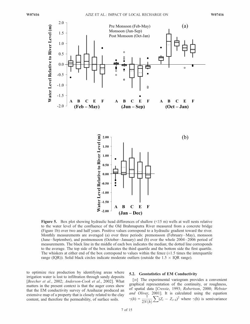
for interval distance class h, Zi is measured sample valueat a point h, Zi+h is measured sample value at a pointi+h and N(h) is the total number of sample couples forthe lag interval h. To obtain the variogram of EMconductivity in Araihazar, distances up to 1000 mseparating two measurements were considered andbinned in 10-m intervals. The results show that thevariance of pairs of EM measurements increases steadilyfrom 0.1 (mS/m)2 for sites 10 m apart to �55 (mS/m)2

at a distance of 400 m (Figure 7). This quantitativelyconfirms our experience from the field that a spatial resolu-tion of �10 m is generally sufficient to capture variations inEM conductivity >1 mS/m. The increase in variance be-tween pairs of determinations up to a distance of 400 m isconsistent with the �500 m scale of several areas ofconsistently high and low conductivity distributed acrossthe study area (Figure 1b). An exponential model was fittedto the variogram by minimizing the sum of squared residualsbetween the model and the observations (RSS = 2266; r2 =0.83; Figure 7). The model was used to contour the EMconductivity data and visually enhance the main features ofthe survey by ordinary block kriging. Ordinary krigingestimates optimally weighted averages for unsampledlocations of an irregularly spaced data set using knowledgeabout the underlying spatial relationships [Cressie, 1993,Robertson, 2000]. A cross-validation comparing estimatedand actual EM conductivities, [y = (1.01 ± 0.01)*x �(0.17 ± 0.05), where y = predicted EM conductivity and x =actual EM conductivity] shows that kriging adequatelycaptures the main features of the variability in the nature ofsurface soils, and therefore permeability, with a standarderror for predicted EM of �2 mS/m based on the standarddeviation of residuals.

5.3. Relation Between EM Conductivity and Asin Groundwater

[21] The contour map of EM conductivity facilitatesvisual comparison with the distribution of As in shallowwells because the two data sets generally do not overlap

(Figure 8). Merging of the two data sets shows, for instance,that interruptions of the diagonal swath of mostly low-Aswells across the northwestern portion of the study area byclusters of high-As wells occur precisely in areas of elevatedEM conductivity. Similarly, two clusters of generally lowAs concentrations to the south are closely delimited by areasof elevated EM conductivity. Overall, the average As contentof shallow wells located within the 10 mS/m contour is 43 ±67 mg/L (n = 606) whereas the average As content of wellslocated outside the same contour is 120 ± 123 mg/L (n =2199). A different way to express the contrast between the twoareas is that 73% of shallow wells located within the 10 mS/mcontour contain <50 mg/L As, whereas this is the case for only

Figure 6. Regression of (a) slurry conductivity and (b) clay fraction integrated to a depth of 200 cm (asdescribed in the text) as a function of EM conductivity for 14 soil profiles collected in the Araihazar studyarea.

Figure 7. Variogram for EM conductivity at an active lagof 1000 m and an active step of 10 m was constructed usingGS + 1 v5.0 (Gamma Design, 2000). Small open circlesshow the experimental variogram; the solid line indicatesthe theoretical variogram.

8 of 15

W07416 AZIZ ET AL.: IMPACT OF LOCAL RECHARGE ON W07416

36% of wells outside the same contour. These observationssuggest that shallow tubewells that meet the Bangladeshstandard for groundwater of 50 mg/L As are unlikely to befound in areas where surface soils contain >10% clay(Figure 4).[22] For a more quantitative comparison between ground-

water As and EM conductivity data, we return to the actualEM data instead of extrapolated values by comparing the Ascontent of each shallow well to the closest EM conductivitymeasurement. To determine the relevant spatial scales toconsider, as determined by the ratio of horizontal to verticalflow, we estimate the distance over which rechargedgroundwater has to travel to reach a depth of 15 m (over

two-thirds of shallow household wells considered in thisstudy are up to 15 m deep). For lateral flow, we start fromannually averaged relative hydraulic head differences be-tween the multilevel sites and the Old Brahmputra River(Figure 5b). In the case of sites A and C, we use the actualdistance of discharge to the river to calculate lateral gra-dients in average hydraulic head (100 and 300, respectively;Table 1). For sites of E and F, we estimate the shortestdistance to a local discharge area to be on the order of 150 mrather than actual distances to the Old Brahmaputra River(Table 1). Vertical hydraulic gradients between the twoshallowest wells at all four sites were previously reportedby Stute et al. [2007]. Using the ratio between horizontal

Figure 8. Comparison of the distribution of As in shallow wells of Araihazar with a contour map of EMconductivity (axis labels in decimal degrees). The EM conductivity surface was mapped using ordinaryblock kriging with a maximum distance of extrapolation of 100 m. Arrows point to the four well nestswhere recharge rates (numbers in m/y) were calculated from 3H-3He ages by Stute et al. [2007].

Table 1. Estimate of Distance Traveled (x = r*z) to Reach a Depth of 15 m at Each of the Multilevel Sites Based on Local Hydraulic

Gradients and Assuming a Horizontal Permeability 10-Fold Greater Than Vertical Permeabilitya

SiteDischargeDistance, m

Horizontal Gradient(ix = dh/dx)

Vertical Gradient(iz = dh/dz)

Horizontal Flow/Vertical Flow(r = 10*ix/iz) Recharge Distance (x), m

A 100 11.0E-04 6.7E-04 16.4 250C 300 9.7E-04 3.3E-04 29.5 450E 150 7.3E-04 1.7E-04 46.5 700F 150 2.0E-04 4.3E-04 4.6 50

aDistance to discharge at sites A and C is the actual distance to the Old Brahmaputra River and an estimate based on local topography at sites E and F.Horizontal head gradients are from annual averages in Figure 5b and vertical head gradients are from Stute et al. [2007].

W07416 AZIZ ET AL.: IMPACT OF LOCAL RECHARGE ON

9 of 15

W07416

and vertical gradients and assuming a vertical anisotropy(Kx/Kz) of 10 [Freeze and Cherry, 1979], distances overwhich recharged groundwater could have traveled to reach adepth of 15 m were then calculated. The results shows thatgroundwater from 15 m depth may have been advectedlaterally by 50 m at site F and by as much as 700 m at site E(Figure 9 and Table 1). This is just an order of magnitudeestimate because the hydraulic gradient between wells nestsand the river is not necessarily linear.[23] On the basis of this simple calculation, we start by

comparing the As content of each shallow well to the closestEM conductivity measurement obtained within a distance of50 m. Linear regression shows a weak but statisticallysignificant relationship (R2 = 0.12, p < 0.001) for 614paired measurements corresponding to an increase in Asconcentrations as a function of EM conductivity (Figure 10a).The relationship remains significant but weakens furtherwhen paired measurements separated by larger distancesare considered (Table 2a). Averaging EM data around thesubset of 504 wells surrounded by at least five measurementsyields a relationship that accounts for a larger proportion ofthe variance (R2 = 0.22). The magnitude of standard devia-tions for five or more EM conductivity measurements within50 m of a well shows that part of the scatter is due to thespatial variability of EM conductivity (Figure 10b). Theoutcome of these regressions does not change markedlywhen considering a smaller or larger minimum number ofEM measurements within a 50 m radius (Table 2b).[24] Vertical profiles of As for nests of monitoring wells

across the study area suggest that EM conductivities couldinstead be compared to the depth gradient of As concen-

trations in shallow aquifers rather than absolute As concen-trations. Concentrations of As start from <50 mg/L in theshallowest monitoring well at each site and typically increasewith depth, gradually at sites associated with low EMconductivities and more rapidly at high conductivity sites(Figure 11). Least squares regression of As as a function of

Figure 9. Diagrams showing the range of distancestraveled by groundwater after being recharged to reach thepumping wells assuming the wells are 15 m deep (verticalscale is exaggerated). The calculation of distances isdiscussed in the text and is shown in Table 1.

Figure 10. Comparison of (a) As content of 614 shallowwells as a function of the closest EM conductivitymeasurement obtained within a distance of 50 m. (b) Asin 504 shallow wells as a function of average EMconductivity consisting of at least 5 measurements withina radius of 50 m. (c) As-depth gradient as a function ofaverage EM conductivities for 145 circles of 50 m radiuswells encompassing at least 5 EM conductivity and at leastfive household wells from which the local depth gradient forAs could be calculated by least squares regression withnonnegativity constraint on the intercept. Horizontal errorbars show the standard deviation of at least five EMconductivity measurements. Vertical error bars show thestandard error in the estimate of the slope of As versus depthby regression for at least five wells.

10 of 15

W07416 AZIZ ET AL.: IMPACT OF LOCAL RECHARGE ON W07416

depth, with a nonnegativity constraint imposed on theintercept, shows that the slope of this relationship increasessystematically as a function of average EM conductivitywithin a radius of 50 m of each of these sites (Figure 12a).The slope of the As-depth relationship increases nearly five-fold across the 7–20 mS/m range in average EMconductivity at these five sites.[25] When considering household wells located within

50 m of each of the five nests of the wells, the depth

gradient in As concentrations is not as well defined, at leastin part because household wells are typically deeper thanthe shallowest of the monitoring wells (Figure 11). Thescatter of the depth trends in As is also considerably largerfor household wells, possibly because of errors in reportedwell depths as well as lateral spatial heterogeneity. Despite

Table 2a. Regression Analysis of As Concentrations as a

Function of EM Conductivity (As = a*EM Conductivity + C) for

Pairs of Data Separated by Various Distancesa

Distance, m a C R2 n

50 4.5 ± 0.5 19.5 ± 9.8 0.12 614100 5.0 ± 0.4 12.7 ± 6.5 0.11 1555200 5.2 ± 0.3 13.9 ± 5.5 0.10 2823500 5.6 ± 0.3 11.1 ± 5.1 0.10 4002

aThe relationships are all highly significant (p < 0.001).

Figure 11. Depth profiles of As at the five well nests (black circles), in order of increasing nearby EMconductivity. Open circles show the depth distribution of As in household wells located within 50 m ofeach well nest. Also shown are least squares regression lines calculated by imposing a nonnegativityconstraint on the intercept.

Table 2b. Regression Analysis of As Concentrations as a Function

of Average EM Conductivity (As = a*Avg EM Conductivity + C)

for Different Minimum Number of EM Conductivity Measurements

Within a Radius of 50 m of Each Wella

Minimum EMReadings a C R2 n

1 5.7 ± 0.6 �0.4 ± 10.8 0.14 6142 6.2 ± 0.6 �4.1 ± 11.2 0.15 5875 7.7 ± 0.7 �29.1 ± 12.1 0.22 50410 8.5 ± 0.8 �38.3 ± 14.1 0.23 39520 8.3 ± 1.0 �34.5 ± 18.5 0.22 246

aThe relationships are all highly significant (p < 0.001).

W07416 AZIZ ET AL.: IMPACT OF LOCAL RECHARGE ON

11 of 15

W07416

these limitations, the data show that the slope of the As-depth relationship based on household wells also generallyincreases as a function of EM conductivity (Figure 12a). Itis unclear, however, why the depth gradients calculatedfrom the household wells are a factor of three below thegradients calculated from the monitoring wells.[26] The results from the area surrounding the five nests

of wells justify a similar comparison of As depth gradientsand EM conductivity within the larger data set. A total of145 out of 614 circles of 50 m radius within the study areacontain at least five household wells and at least 5 EMconductivity measurements (Figure 1b). Although there isconsiderable scatter, the relationship between EM conduc-tivities and the As-depth gradient is highly significant (p <0.001) and accounts for 50% of the variance (Figure 10c).Whereas the proportion of the variance that can beaccounted for depends on the number of wells or EMmeasurements used for averaging, the relationship between

As-depth gradients and EM conductivity itself is not verysensitive (Table 3). In the next two sections we examinewhy the rate of increase of As concentrations with depth inshallow aquifers of Araihazar might depend on the claycontent of surface soil inferred from EM conductivity.

5.4. Relation Between EM Conductivity andGroundwater Age

[27] Independently of its relation to As, it is worthwhileto compare the distribution of EM conductivity withgroundwater ages at the five nests of wells within the studyarea where the 3H-3He dating technique was applied. Stuteet al. [2007] showed that the time elapsed since rechargeincreases with depth at all five sites, but at a rate that variesconsiderably from one nest of wells to the other. At the twosites located within an area of low EM conductivity (sites Cand F), the age of groundwater interpolated to a depth of12 m (40 ft) is 3 to 4 years. In contrast, the age ofgroundwater at the same depth at the two sites surroundedby regions of high EM conductivity (sites A and B) is 18to 19 years. Considering recharge rates estimated by Stuteet al. [2007] from the vertical 3H/3He age gradient for theshallowest two samples at each well nest confirms thatrecharge is correlated with EM conductivity (Figure 12b)and shows that sandy deposits that extend essentially to thesurface are recharged an order of magnitude faster thanshallow aquifers that are capped by a relatively imperme-able layer of fine-grained sediments.[28] Similar conclusions were drawn from a combination

of recharge estimates and electromagnetic measurements insoutheastern Australia, albeit under considerably drier con-ditions than in Bangladesh [Cook et al., 1992]. The samestudy predicts an exponential relationship between rechargeand EM conductivity that may be consistent with ourobservations, even if a linear relationship could equally beinferred from our limited data (Figure 12b). The observa-tions from Araihazar are more directly related to recentwork conducted in the Himalayan foothills of India [Israil etal., 2006]. In that study, the penetration of 3H injected insurface soil by infiltration of precipitation and return seep-age from irrigated fields was shown to increase with the

Figure 12. (a) Comparison of average EM conductivitiesand As-depth gradients calculated from multilevel well sites(black circles) and household wells (open circles) within50 m of each well nest. Error bars indicate the standarddeviation of EM conductivities and the uncertainty in theAs-depth slope (1-sigma), respectively. (b) Comparison ofaverage EM conductivities and recharge rates (estimated byStute et al., 2007) at the five well nests.

Table 3. Regression Analysis of As-Depth Gradients as a

Function of Average EM Conductivity (As-Depth Gradients =

a*Avg EM Conductivity + C) for Different Minimum Number of

EM Conductivity Measurements and Wells Within a Radius of 50

m of Each Wella

Min #of Wells

Min #of EM a C R2 n

3 1 0.43 ± 0.03 �0.70 ± 0.69 0.37 2763 5 0.42 ± 0.04 �0.43 ± 0.73 0.37 2333 10 0.40 ± 0.04 0.07 ± 0.88 0.32 1803 20 0.39 ± 0.06 0.14 ± 1.12 0.29 1225 1 0.43 ± 0.03 �1.19 ± 0.60 0.53 1805 5 0.41 ± 0.03 �0.85 ± 0.72 0.50 1455 10 0.40 ± 0.04 �0.33 ± 0.91 0.44 1095 20 0.41 ± 0.06 �0.74 ± 1.17 0.41 793 1 0.43 ± 0.03 �0.70 ± 0.69 0.37 2765 1 0.43 ± 0.03 �1.19 ± 0.60 0.53 18010 1 0.44 ± 0.03 �2.05 ± 0.69 0.76 63

aAs-Depth gradients were calculated using non-negativity constrainedleast squares method. The relationships are all highly significant (p < 0.001).

12 of 15

W07416 AZIZ ET AL.: IMPACT OF LOCAL RECHARGE ON W07416

permeability of the soil, as determined by electrical resis-tivity measurements. Our observations from Araihazar pro-vide further quantitative evidence that variations in surfacepermeability strongly influence the rate of local recharge ofshallow fluvio-deltaic aquifers.[29] To what extent are shallow aquifers of Araihazar

affected by irrigation pumping? Mechanized irrigation wellsin the area are typically constructed with filters that extendfrom �6 to 21 m (20 to 70 ft) depth. A total of 125mechanized irrigation wells were identified during a sys-tematic survey of a 14 km2 portion of the study area(Figure 1a), approximately 40% of which are used forgrowing rice according to satellite imagery [Van Geen etal., 2003a]. A crop of rice requires �1 m of irrigation waterper year [Meharg and Rahman, 2003; Huq et al., 2006].This requirement, combined with the density of irrigationwells and typical pumping rates of 20–30 L/s [Harvey etal., 2006; van Geen et al., 2006], is consistent withirrigation wells operating 3–4 h each day during fourmonths of the dry season. Stute et al. [2007] concludedthat vertical recharge rates in the same study area rangefrom 0.05 to 1 m/a using two independent methods: bymeasuring vertical head gradients and hydraulic conductiv-ities and by 3H-3He dating of shallow groundwater. Com-parison with the water requirement for growing riceindicates that the scale of irrigation withdrawals fromshallow aquifers during the dry season is at least compara-ble to that of annual vertical recharge [Harvey et al., 2002,2006]. Irrigation could therefore significantly affect thedistribution of shallow groundwater properties in the studyarea.[30] Is the spatial relation between groundwater age

profiles and surface permeability inferred from EM conduc-tivity consistent with plausible flow lines for recharge?Based on the simple calculation of the lateral advection ofrecharged water, in areas where shallow groundwater isyoung should roughly correspond to areas where surfacepermeability inferred from EM conductivity is low (Figure 9and Table 1). In contrast, in areas where surface permeabil-ity is low, shallow groundwater that is older in agerecharged further away (Figure 9). Therefore the connectionbetween groundwater age and surface permeability might bemore complex because of variable flow paths leading frommore distant recharge areas. This might explain the weakrelationship between surface EM conductivity and ground-water As concentrations in wells (Figure 10a). This mightalso be the cause of the considerable scatter of the relation-ship between EM conductivity and As-depth gradients thatremains even after properties are averaged within a radius of50 m (Figure 10c).[31] In a complementary study conducted in the same

area, Weinman et al. [2008] have shown that low-EMconductivity areas of Araihazar are typically associated withhigh energy, sandy depositional environments such as relictchannel levees and bars, on the basis of elevation surveysand grain-size analysis of a considerable number of augercores. In contrast, the geology of several of the very high-EM conductivity areas was interpreted as an indication ofabandoned channels filled with fine-grained sediment. Onthe basis of these findings, the variability of recharge ofshallow aquifers in Araihazar can therefore also be relatedthe depositional history of fluvio-deltaic environments.

5.5. Implications for Groundwater As

[32] Stute et al. [2007] showed that As concentrations inshallow aquifers of Araihazar increase roughly linearlywith the age of the groundwater at a rate of �20 mg/L per a.Dissolved As concentrations are typically well below 50 mg/LinBangladesh pond and river water and, we can safely assume,also in precipitation [BGS/DPHE, 2001]. Vertical rechargefrom surface water bodies and precipitation would thereforetend to dilute any As that is released from the sediment atdepth in reducing aquifers. Recharge with precipitation orsurface water also supplies oxidants in the form of dissolvedoxygen and nitrate that inhibit the reductive dissolution of Feoxyhydroxides [BGS/DPHE, 2001; Horneman et al., 2004].Both dilution and inhibition of reductive dissolution areconsistent with the observation that dissolved As concen-trations in the shallowest aquifers of Araihazar decrease asthe rate of local recharge increases.[33] Water levels in the confluent of the Old Brahmputra

River are rarely higher than in shallow aquifers of the area(Figure 5). Lateral flow across river banks may also beinhibited by fine-grained river bottom and overbank depos-its, suggesting that rivers may be a relatively unimportantsource of recharge in Araihazar. Perhaps for that reasonalso, the majority of shallow tubewells along the banks ofthe Old Brahmaputra River and its confluent are elevated inAs (Figure 1a). The situation may be different in an areasuch as Munshiganj where there is less opportunity forvertical recharge because of the presence of an uninterruptedclay layer at the surface [Harvey et al., 2006].[34] It remains unclear to what extent the relationship

between surface permeability, vertical recharge, and Asconcentrations reflects a steady source within the sedimentthat is diluted by groundwater flow or the flushing of shallowaquifers of their initial As content over time [Radloff et al.,2007; Stute et al., 2007; van Geen et al., 2008]. Suchuncertainties make it difficult to speculate on the impact thatthe onset of irrigation pumping in recent decades may havehad on the distribution of As in shallow groundwater. If theonset of irrigation pumping enhanced vertical recharge, theweight of the evidence would suggest that at least in Arai-hazar this resulted in lower rather than higher As concen-trations in shallow aquifers [Harvey et al., 2002, 2006;Klump et al., 2006; Stute et al., 2007].

6. Conclusion

[35] The geophysical data presented in this study reveal arelationship between the permeability of surface soils andthe distribution of both groundwater ages and As concen-trations in shallow aquifers of Araihazar. The observationsunderline the importance of vertical recharge of precipita-tion, monsoonal flooding, and irrigation seepage water forsetting the properties of shallow groundwater including As.Hydrological processes must therefore be considered tounravel widespread but spatially variable As enrichmentsin South Asian deltaic aquifers, in conjunction with the stillpoorly understood biogeochemical processes that lead to therelease of As to groundwater.

[36] Acknowledgments. Columbia University and the University ofDhaka’s research and mitigation work in Araihazar since 2000 has beensupported by NIEHS Superfund Basic Research Program grant NIEHS 1P42 ES10349, Fogarty International Center grant NIEHS 5-D43 TW05724-

W07416 AZIZ ET AL.: IMPACT OF LOCAL RECHARGE ON

13 of 15

W07416

01, NSF grant EAR 03-45688, NSF grant EAR 04-33886, and the EarthInstitute at Columbia University. This is Lamont-Doherty Earth Observa-tory publication number 7170.

ReferencesAhmed, M. F., S. Ahuja, M. Alauddin, S. J. Hug, J. R. Lloyd, A. Pfaff,T. Pichler, C. Saltikov, M. Stute, and A. van Geen (2006), Ensuringsafe drinking water in Bangladesh, Science, 314, 1687–1688.

Anderson-Cook, C. M., M. M. Alley, J. K. F. Roygard, R. Khosla, R. B.Noble, and J. A. Doolittle (2002), Differentiating soil types using elec-tromagnetic conductivity and crop yield maps, Soil Sci. Soc. Am. J.,66(5), 1562–1570.

Banton, O., M. K. Seguin, and M. A. Cimon (1997), Mapping field-scalephysical properties of soil with electrical resistivity, Soil Sci. Soc. Am. J.,61, 1010–1017.

Beecher, H. G., I. H. Hume, and B. W. Dunn (2002), Improved method forassessing rice soil suitability to restrict recharge, Aust. J. Exp. Agric.,42(3), 297–307.

BGS and DPHE (2001), Arsenic contamination of groundwater in Bangla-desh, edited by D. G. Kinniburgh and P. L. Smedley, vol. 2, Final Report,BGS Technical Report WC/00/19, British Geological Survey, Keyworth,U. K.

Brammer, H. (1996), The Geography of the Soils of Bangladesh, 287 pp.,University Press, Ltd., Dhaka, Bangladesh.

Chakraborty, A. K., and K. C. Saha (1987), Arsenical dermatosis fromtubewell water in West Bengal, Indian J. Med Res., 85, 326–334.

Cook, P. G., and G. R. Walker (1992), Depth profiles of electrical con-ductivity from linear-combination of electromagnetic induction measure-ments, Soil Sci. Soc. Am. J., 56(4), 1015–1022.

Cook, P. G., M. W. Hughes, G. R. Walker, and G. B. Allison (1989), Thecalibration of frequency-domain electromagnetic induction meters andtheir possible use in recharge studies, J. Hydrol., 107(1–4), 251–265.

Cook, P. G., G. R. Walker, G. Buselli, I. Ports, and A. R. Dodds (1992), Theapplication of electromagnetic techniques to groundwater recharge inves-tigations, J. Hydrol., 130, 201–229.

Cressie, N. A. C. (1993), Statistics for Spatial Data, Rev Ed. John Wiley,Hoboken, N. J.

Dalgaard, M., H. Have, and H. Nehmdahl (2001), Soil clay mappingby measurement of electromagnetic conductivity, in Proceedings ofThird European Conference on Precision Agriculture, 367–372, AgroMontpellier, France.

Dhar, R. K., et al. (1997), Ground water arsenic calamity in Bangladesh,Curr. Sci., 73(1), 48–59.

Doolittle, J. A., K. A. Sudduth, N. R. Kitchen, and S. J. Indorante (1994),Estimating depths to clay pans using electromagnetic induction methods,J. Soil Water Conserv., 49, 572–575.

Doolittle, J., M. Petersen, and T. Wheeler (2001), Comparison of twoelectromagnetic induction tools in salinity appraisals, J. Soil Water Con-serv; Third Quarter 2001, 56(3), 257.

Doolittle, J. A., S. J. Indorante, D. K. Potter, S. G. Hefner, and W. M.McCauley (2002), Comparing three geophysical tools for locating sandblows in alluvial soils of southeast Missouri, J. Soil Water Conserv.,57(3), 175.

Durlesser, H. (1999), Bestimmung der Variation Bodenphysikalischer Para-meter in Raum und Zeit mit electro-magnetischen Induktionsverfahren,(in German) FAM-Bericht 35; 121 pp. (Determination of soil physicalproperties variation in space and time using electromagnetic inductionmethods) (Shaker Verlag Aachen, Germany (FAM-Bericht; Bd. 53) to-gether Diss. Techn. Univ. Munchen)

Fergusson, J. (1863), On recent changes in the delta of the Ganges, Quart.J. Geol. Soc., 19, 321–354.

Freeze, R. A., and J. A. Cherry (1979), Groundwater, xvi, 604 pp., PearsonEducation Group, Englewood Cliffs, N. J.

Geonics Limited (1992), EM31 operating manual (for models with twodigital meters), Geonics Ltd., Mississauga. Ontario.

Goodbred, S. L., and S. A. Kuehl (2000), The significance of large sedi-ment supply, active tectonism, and eustasy on margin sequence develop-ment: Late Quaternary stratigraphy and evolution of the Ganges-Brahmaputra delta, Sediment. Geol., 133(3–4), 227–248.

Goodbred, S. L., S. A. Kuehl, M. S. Steckler, and M. H. Sarker (2003),Controls on facies distribution and stratigraphic preservation in theGanges-Brahmaputra delta sequence, Sediment. Geol., 155, 301–316.

Harvey, C. F., et al. (2002), Arsenic mobility and groundwater extraction inBangladesh, Science, 298(5598), 1602–1606.

Harvey, C. F., et al. (2006), Groundwater dynamics and arsenic contamina-tion in Bangladesh, Chem. Geol., 228(1–3), 112–136.

Hedley, C. B., I. Y. Yule, C. R. Eastwood, T. G. Shepherd, and G. Arnold(2004), Rapid identification of soil textural and management zones usingelectromagnetic induction sensing of soils, Aust. J. Soil Res., 42(4), 389–400.

Hendrickx, J. M. H., B. Baerends, Z. I. Rasa, M. Sadig, and M. A.Chaudhry (1992), Soil salinity assessment by electromagnetic inductionof irrigated land, Soil Sci. Soc. Am. J., 56, 1933–1941.

Horneman, A., et al. (2004), Arsenic mobilization in Bangladesh ground-water decoupled from dissolution of iron oxyhydroxides. part I: Evidencefrom borehole cuttings, Geochimic. Cosmochim. Acta, 68(17), 3459–3473.

Huq, S. M. I., J. C. Joardar, S. Parvin, R. Correll, and R. Naidu (2006),Arsenic contamination in food-chain: Transfer of arsenic into food ma-terials through groundwater irrigation, J. Health Population Nutrition,24(3), 305–316.

Israil, M., M. Al-hadithi, D. C. Singhal, and B. Kumar (2006), Ground-water-recharge estimation using a surface electrical resistivity method inthe Himalayan foothill region, India, Hydrogeol. J., 14(1–2), 44–50.

Johnson, C. K., J. W. Doran, H. R. Duke, B. J. Wienhold, K. M. Eskridge,and J. F. Shanahan (2001), Field-scale electrical conductivity mappingfor delineating soil condition, Soil Sci. Soc. Am. J., 65, 1829–1837.

Kitchen, N. R., K. A. Sudduth, and S. T. Drummond (1996), Mapping ofsand deposition from 1993 midwest floods with electromagnetic induc-tion measurements, J. Soil Water Conserv., 5(1), 336–340.

Klump, S., R. Kipfer, O. A. Cirpka, C. F. Harvey, M. S. Brennwald, K. N.Ashfaque, A. B. M. Badruzzaman, S. J. Hug, and D. M. Imboden(2006), Groundwater dynamics and arsenic mobilization in Bangladeshassessed using noble gases and tritium, Environ. Sci. Technol., 40(1),243–250.

Lesch, S. M., D. J. Strauss, and J. D. Rhoades (1995), Spatial prediction ofsoil salinity using EM induction techniques, Water Resour. Res., 31(2),373–386.

McArthur, J. M., et al. (2004), Natural organic matter in sedimentary basinsand its relation to arsenic in anoxic ground water: The example of WestBengal and its worldwide implications, Appl. Geochem., 19(8), 1255–1293.

McNeill, J. D. (1980a), Electromagnetic terrain conductivity measurementat low induction numbers, Technical note TN-6, Geonics Ltd, Toronto.

McNeill, J. D. (1980b), Electrical Conductivity of Soils and Rocks, Tech-nical Note TN-5, Geonics Ltd: Ontario.

McNeill, J. D. (1986), Rapid, accurate mapping of soil salinity using elec-tromagnetic ground conductivity meters, Technical Note TN-18, GeonicsLimited, Ontario, Canada.

McNeill, J. D. (1990), Use of electromagnetic methods for ground-waterstudies, in Geotechnical and Environmental Geophysics: I. Review andTutorial, edited by S. N. Ward pp. 191–218, Society of ExplorationGeophysicists, Tulsa, OK.

Meharg, A. A., and M. Rahman (2003), Arsenic contamination of Bangla-desh paddy field soils: Implications for rice contribution to arsenic con-sumption, Environ. Sci. Technol., 37, 229–234.

Morgan, J. P., and W. C. McIntire (1959), Quaternary geology of the BengalBasin, East Pakistan and India, Bull. Geol. Soc. Am., 70, 319–342.

Nickson, R., J. McArthur, W. Burgess, K. M. Ahmed, P. Ravenscroft, andM. Rahman (1998), Arsenic poisoning of Bangladesh groundwater,Nature, 395(6700), 338.

Pellerin, L. (2002), Applications of electrical and electromagnetic methodsfor environmental and geotechnical investigations, Surv. Geophys., 23,101–132.

Pettersson, J. K., and D. C. Nobes (2003), Environmental geophysics atScott Base: Ground penetrating radar and electromagnetic induction astools for mapping contaminated ground at Antarctic research bases, ColdReg. Sci. Technol., 918, 1–9.

Polizzotto, M. L., C. F. Harvey, G. C. Li, B. Badruzzman, A. Ali,M. Newville, S. Sutton, and S. Fendorf (2006), Solid-phases and deso-rption processes of arsenic within Bangladesh sediments, Chem. Geol.,228(1–3), 97–111.

Radloff, K. A., Z. Q. Cheng, M. W. Rahman, K. M. Ahmed, B. J. Mailloux,A. R. Juhl, P. Schlosser, and A. van Geen (2007), Mobilization of arsenicduring one-year incubations of grey aquifer sands from Araihazar, Ban-gladesh Environ. Sci. Technol., 41(10), 3639–3645.

Ravenscroft, P., W. G. Burgess, K. M. Ahmed, M. Burren, and J. Perrin(2005), Arsenic in groundwater of the Bengal Basin, Bangladesh: Dis-tribution, field relations, and hydrogeological setting, Hydrogeol. J.,13(5–6), 727–751.

Rhoades, J. D. (1981), Predicting bulk soil electrical-conductivity versussaturation paste extract electrical-conductivity calibrations from soilproperties, Soil Sci. Soc. Am. J., 45(1), 42–44.

14 of 15

W07416 AZIZ ET AL.: IMPACT OF LOCAL RECHARGE ON W07416

Rhoades, J. D., and D. L. Corwin (1981), Determining soil electrical con-ductivity–depth relations using an inductive electromagnetic soil con-ductivity meter, Soil Sci. Soc. Am. J., 45, 255–260.

Rhoades, J. D., S. M. Lesch, P. J. Shouse, and W. J. Alves (1989), Newcalibrations for determining soil electrical-conductivity-depth relationsfrom electromagnetic measurements, Soil Sci. Soc. Am. J., 53(1), 74–79.

Robertson, G. P. (2000), GS+: Geostatistics for the Environmental Science,Gamma Design Software, Michigan, USA.

Stute, M., et al. (2007), Hydrological control of As concentrations in Ban-gladesh groundwater, Water Resour. Res., 43, W09417, doi:10.1029/2005WR004499.

Triantafilis, J., and S. M. Lesch (2005), Mapping clay content variationusing electromagnetic induction techniques, Comput. Electron. Agric.,46, 203–237.

Triantafilis, J., M. F. Ahmed, and I. O. A. Odeh (2002), Application of amobile electromagnetic sensing system (MESS) to assess cause andmanagement of soil salinization in an irrigated cotton-growing field, SoilUse Manage., 18, 330–339.

Umitsu, M. (1993), Late quaternary sedimentary environments and land-forms in the Ganges delta, Sediment. Geol., 83(3–4), 177–186.

van Geen, A., Z. Cheng, A. A. Seddique, M. A. Hoque, A. Gelman, J. H.Graziano, H. Ahsan, F. Parvez, and K. M. Ahmed (2005), Reliability of acommercial kit to test groundwater for arsenic in Bangladesh, Environ.Sci. Technol., 39(1), 299–303.

van Geen, A., et al. (2002), Promotion of well-switching to mitigate thecurrent arsenic crisis in Bangladesh, Bull. World Health Organization,80(9), 732–737.

van Geen, A., K. M. Ahmed, A. A. Seddique, and M. Shamsudduha(2003a), Community wells to mitigate the current arsenic crisis inBangladesh, Bull. World Health Organization, 82, 632–638.

van Geen, A., et al. (2003b), Spatial variability of arsenic in 6000 tube wellsin a 25 km2 area of Bangladesh, Water Resour. Res., 39(5), 1140,doi:10.1029/2002WR001617.

van Geen, A., Y. Zheng, Z. Cheng, Y. He, R. K. Dhar, J. M. Garnier,J. Rose, A. Seddique, M. A. Hoque, and K. M. Ahmed (2006),Impact of irrigating rice paddies with groundwater containing arsenicin Bangladesh, Sci. Total Environ., 367(2–3), 769–777.

van Geen, A., et al. (2008), Flushing history as a hydrogeological controlon the regional distribution of arsenic in shallow groundwater of theBengal Basin, Environ. Sci. Technol., 42, 2283–2288.

Vaughan, P. J., S. M. Lesch, D. L. Corwin, and D. G. Cone (1995), Watercontent effect on soil salinity prediction: A geostatistical study usingcokriging, Soil Sci. Soc. Am. J., 59, 1146–1156.

Waine, T. W., B. S. Blackmore, and R. J. Godwin (2000), Mapping avail-able water content and estimating soil textural class using electro-mag-netic induction, in Proceedings of EurAgEng, Paper 00-SW-044, AgEng2000, Silsoe Research Institute, Warwick, UK.

Webster, R., and M. A. Oliver (2001), Geostatistics for EnvironmentalScientists, 2nd Ed. John Wiley, Hoboken, N. J.

Weinman, B., S. L. Goodbred, Y. Zheng, Z. Aziz, A. Singhvi, Y. C. Nagar,S. Steckler, and A. van Geen (2008), Contributions of floodplain strati-graphy and evolution to the spatial patterns of groundwater arsenic inAraihazar, Bangladesh, Geol. Soc. Am. Bull.

Williams, B. G., and D. Hoey (1987), The use of electromagnetic inductionto detect the spatial variability of the salt and clay contents of soil, Aust.J. Soil Res., 25, 21–28.

Yu, W. H., C. M. Harvey, and C. F. Harvey (2003), Arsenic in groundwaterin Bangladesh: A geostatistical and epidemiological framework for eval-uating health effects and potential remedies, Water Resour. Res., 39(6),1146, doi:10.1029/2002WR001327.

Zheng, Y., et al. (2005), Geochemical and hydrogeological contrasts be-tween shallow and deeper aquifers in two villages of Araihazar, Bangla-desh: Implications for deeper aquifers as drinking water sources,Geochim. Cosmochim. Acta, 69, 5203–5218.

����������������������������K. M. Ahmed, M. A. Hoque, and M. Shamsudduha, Department of

Geology, University of Dhaka, Dhaka 1000, Bangladesh.

Z. Aziz, Department of Earth and Environmental Sciences, ColumbiaUniversity, NY 10027, USA. (aziz@ldeo.columbia.edu)

I. Gavrieli, Geological Survey of Israel, Jerusalem 95501, Israel.

S. Goodbred and B. Weinman, Earth & Environmental Sciences,Vanderbilt University, Nashville, TN 37235, USA.

A. Horneman, M. Steckler, and A. van Geen, Lamont-Doherty EarthObservatory of Columbia University, Palisades, NY 10964, USA.

M. Stute, Department of Environmental Sciences, Barnard College, NewYork, NY 10027, USA.

R. Versteeg, Idaho National Laboratory, Idaho Falls, ID, USA.

Y. Zheng, Earth and Environmental Sciences, Queens College, CityUniversity of New York, Flushing, NY 11367, USA.

W07416 AZIZ ET AL.: IMPACT OF LOCAL RECHARGE ON

15 of 15

W07416