Impact of Income Shocks on child health outcomes in Malawi

WRITING SAMPLE

Impact of Income Shocks on Child Health: A case

study of Malawi

Devjit Roy Chowdhury

11/30/2013

JEL Codes: I00, O10.

Keywords : Malawi, Child Health, Income Shocks, Drought

Abstract: Utilizing a recent cross-sectional dataset for Malawi I am able to establish a relationship

between income and health measures. From the empirical results it is observed that income shocks are

significant for child health and this result conforms to the established literature. I also observe that certain

age groups within infants and children are affected significantly more than others. This result has

important policy implications as it identifies the target group who are most sensitive to such idiosyncratic

shocks.

1

“The first wealth is health.” - Ralph Waldo Emerson

1. Introduction

This study aims to measure the impact of income shocks on child anthropometric

measures like weight, height and BMI for infants and children in Malawi.

Located at South Eastern Africa, Malawi is a landlocked country with a land area

of 94,276 sq km and population of 13,066,320 (Malawi Census 2008). In land area,

Malawi occupies the 98th position i.e. between North Korea and Benin. It is one

of the poorest countries in the world without a violent internal conflict and a GDP

per capita of 653 US dollars (PPP) 2006 (OECD African Economic Outlook, 2007).

Agriculture is of prime importance for vast majority of Malawi with agricultural

population consisting of 80 percent of the total population. Major crops grown in

Malawi are tobacco, a cash crop, accounting for more than half of all export

revenues. Sugar, coffee and tea also earn export revenues and maize and cassava

are the important food crops. Farmers plant on small plots by hand at the

beginning of the rainy season in October/November, but with little irrigated land,

people are vulnerable to increasingly erratic rainfall.

Given the high incidence of poverty in the country and over reliance on

agriculture an immediate question that crops up is how do households cope with

negative income shocks? In this paper I look at one of the possible channels of an

impact of such a shock i.e. its effect on health outcomes of infants and children.

For this purpose I look at a cross-section survey conducted in Malawi between

2009 and 2010. The survey is at the household level where they ask whether the

household has been affected by droughts or irregular rains in the last year.

http://thinkexist.com/quotes/ralph_waldo_emerson/

2

Income is given by the total consumption at the household level. Here health

outcomes are measured as Body Mass Index (BMI), weight and height. Given the

endogeneity present in the income variable I proxy it with the instrument rain

shock. I observe for certain age groups income shocks do matter for weight and

there is a significant and strong relationship between the variables.

The paper is arranged as follows- Section 2 gives the literature on weather shocks

and its impact on early childhood health measures, Section 3 describes the data

used for this study, Section 4 gives the empirical specification utilized, Section 5

gives the main results while Section 6 concludes.

2. Background

The idea of using weather shock as an instrument variable comes from Miguel

(2005) who utilized rainfall variation as an instrument to estimate the impact of

income shocks in determining murder rate of “witches” in a rural Tanzanian

district. Miguel reasoned that in areas heavily dependent on rain-fed agriculture,

extreme rainfalls causes a significant drop in income leading to incidence of

murders of elderly women in the area. In his empirical estimation he lacked

household income as a variable and as a result he conducts reduced form

estimation for rainfall variation on witch murders.

Child health outcomes during a drought have been studied extensively. It has

been observed from a panel study in Zimbabwe, for children aged 12 to 24

months the advent of a drought lowers the annual growth rates of height by 1.5

3

and 2 centimeters (Hoddinott and Kinsey, 2001). Catch up growth for these

children are limited and this effect is permanent in nature.

A recent study (Kudamatsu et al, 2012) on weather events and its consequence on

mortality for African countries shows that Infants in arid areas who experience

droughts when in utero face a higher risk of death and the risks are greater if they

are born during the “hungry” season i.e. around the start of the rains.

Early life health outcomes are important for schooling and productivity outcomes.

Alderman et al (2003) explore the long term consequences of early childhood

malnutrition for a long term panel data set for Zimbabwe and use drought shocks

and civil war conflicts as instruments for difference in preschool nutrition among

siblings. Height-for-age is used as a measure for childhood chronic malnutrition

and higher values of this measure are associated with a higher number of

schooling grades completed. Another paper in this literature is Maccini and Yang

(2009) who look at early life rainfall data for Indonesia and conclude that higher

rainfall results in improved health, schooling, and socioeconomic status for

women. Their findings

For Malawi, Makoka (2008) examines the impact of droughts on household

vulnerability. He considers the panel component from the previous survey (IHS,

2004) consisting of two periods and shows that households exposed to droughts

in both periods are twice more vulnerable than households exposed to drought

for one period, where framework of vulnerability is expected poverty.

4

This study contributes to the child health literature by estimating the impact of

income shocks on child health as measured by height, weight and BMI for children

in Malawi. Given the high dependence of citizens of Malawi on rain-fed

agriculture as a primary source of employment and subsistence this study is both

necessary and important for obtaining a measure of impact on infant and child

health after a rain shock. Another unique feature of this study is that it uses the

Third Integrated Household Survey for Malawi, a dataset that is very recent with

the sample period being March 2009 to March 2010.

3. Data

The data source for this paper is the Third Integrated Household Survey,

2010/2011 collected by the National Statistical Office of Malawi. It was carried

out for a period of twelve months from March 2009 to March 2010. Sampling

framework was based on a stratified two stage sampling design based on the

2008 Malawi Population and Housing Census. This dataset excludes the island

district of Likoma and is representative at national, district, rural and urban levels.

The purpose of this survey is multifold, it provides information on key welfare and

socio-economic indicators, review of the Malawi Growth Development Strategy

and the Millennium Development Goals, understanding households living

conditions, estimate of total household expenditure, updating household weights

on consumption for calculation of Consumer Price Index and detailed agricultural

activities (IHS3 Report, 2012). Four types of questionnaires were administered

during the survey which is the household, agriculture, fishing and community

questionnaire.

5

The total sample size of the survey is 12,271 households consisting of 56,218

individuals. For the study I consider the household questionnaire for the variables

of interest. The anthropometric measures for children are contained in section V

of this questionnaire. Here both weight and height measures of children are

available in kilograms and meters respectively. Children aged below 24 months

old are measured lying down. BMI is calculated by dividing weight by the square

of height.

In section U of the survey the households were asked whether they had been

affected by adverse shocks in the last twelve months. Some of the shocks were

weather shocks such as droughts, landslides, earthquakes. Among these shocks,

the largest response was for droughts with 37.8 percent of households

responding in affirmative to being affected by droughts. This was far larger than

the other weather shocks; floods (3.5 percent) and earthquakes (2.9 percent).

Since my interest is to investigate health outcomes of children who are most

vulnerable to such weather shocks I look at a subsection of the data i.e. for

children aged up to 48 months old. I am left with observations for 4684 children.

For the study total consumption per capita is considered as a proxy for income. I

also consider food consumption per capita as another measure of income. These

two variables are in the summary data for the survey.

Given the district level information present in the survey and my interest in rural

households coping with income shocks, I excluded cities from the survey. These

cities were Mzuzu City, Lilongwe city, Zomba city and Blantyre city. Southern

regions of Malawi in 2009/2010 experienced high food insecurity. This food

insecurity arose from prolonged periods of dry spells, before the survey period.

6

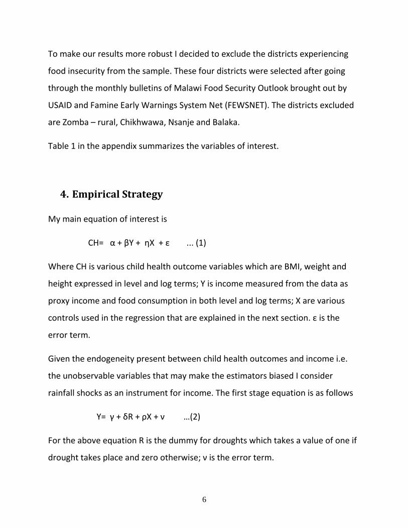
To make our results more robust I decided to exclude the districts experiencing

food insecurity from the sample. These four districts were selected after going

through the monthly bulletins of Malawi Food Security Outlook brought out by

USAID and Famine Early Warnings System Net (FEWSNET). The districts excluded

are Zomba – rural, Chikhwawa, Nsanje and Balaka.

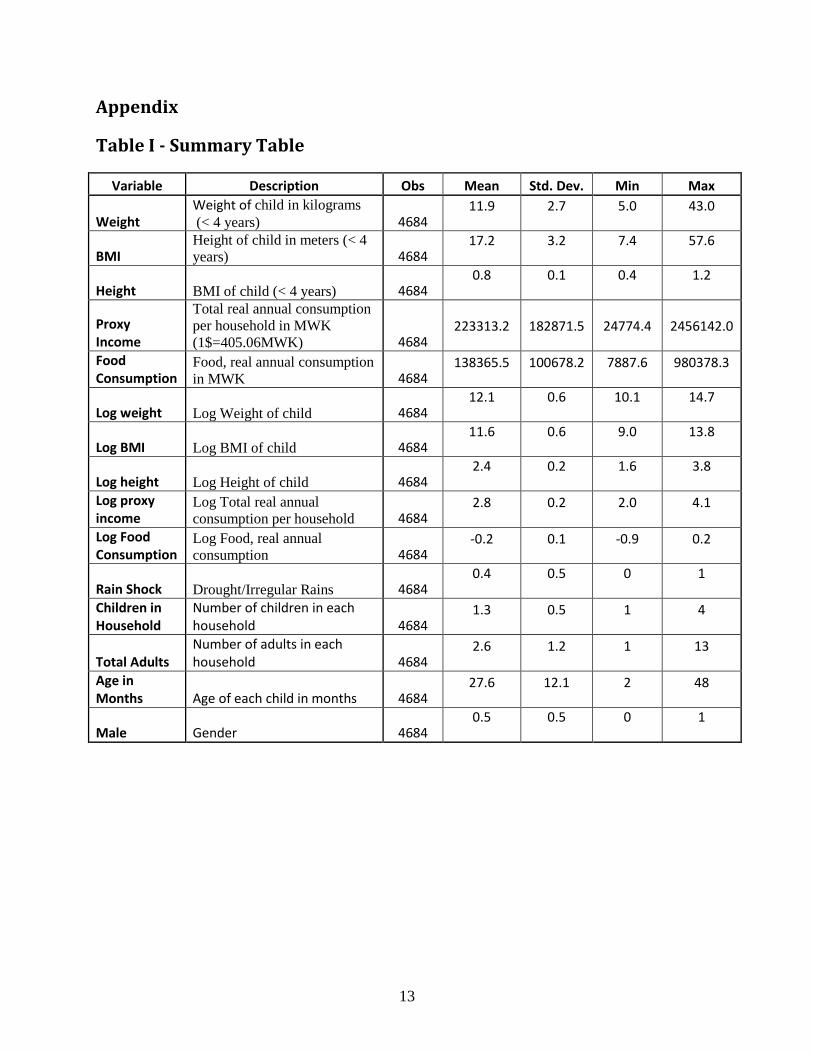
Table 1 in the appendix summarizes the variables of interest.

4. Empirical Strategy

My main equation of interest is

CH= α + βY + ηX + ε ... (1)

Where CH is various child health outcome variables which are BMI, weight and

height expressed in level and log terms; Y is income measured from the data as

proxy income and food consumption in both level and log terms; X are various

controls used in the regression that are explained in the next section. ε is the

error term.

Given the endogeneity present between child health outcomes and income i.e.

the unobservable variables that may make the estimators biased I consider

rainfall shocks as an instrument for income. The first stage equation is as follows

Y= γ + δR + ρX + ν …(2)

For the above equation R is the dummy for droughts which takes a value of one if

drought takes place and zero otherwise; ν is the error term.

7

5. Results

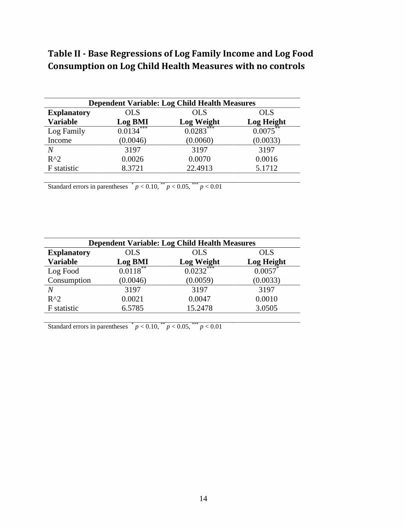
5.1 Base Regressions

To estimate the importance of income on health measures I estimate equation (1)

without the controls for all children below three years old for all health measures.

Family income is considered to be total consumption per household. As seen in

Table II given in the appendix a percent rise in family income results in almost

0.03 percent rise in weight, .0075 percent rise in height and 0.01 percent rise in

BMI and these coefficients are significant. To interpret these results say for

weight, the mean of weight is 10.8910 kilograms for children below four years

old; a 0.03 percent rise would imply an increase of 33 grams. Though in absolute

terms these results may not mean much but at the margins this difference could

lead to a child being malnourished or undernourished. Here the relative is more

important than the absolute.

These results are in line with the existing literature of households with high

family income will have healthy children and gives me confidence in exploring this

issue in further detail. We also run the same regression for log of food

consumption and obtain similar results. It is given along with regression of log of

family income in Table II in the appendix.

8

5.2 Reduced Form Regressions

For the reduced form regressions I add controls for the regression. The controls I

consider are the gender of the child, number of children in the household,

number of adults in the household and the age in months of the respondent.

As mentioned in the data section I drop the four city districts and four food

insecure districts. Malawi has 31 districts and dropping these eight districts leaves

me with 23 districts. I also consider the month of the survey fixed effects as I

wanted to control for children interviewed in “hungry” months. I estimate

reduced forms for the estimation where my dependent variable is various health

measures and the independent variable are rain shocks, the controls, district fixed

effects (dummy variables for 22 districts) and the month of interview fixed effect

(dummy variables for 11 months). I observe the independent variable of rain

shock turns out be insignificant. A possible reason for this occurrence could be the

presence of children above a certain age whose health is unaffected by these

shocks. To investigate this issue I partition my regression into subsamples

according to the different age ranges. I consider six age ranges which are children

between 0 to 24 months, children between 0 to 18 months, children between 13

to 24 months, children between 19 to 24 months, children between 0 to 24

months and children between 0 to 30 months. I double check the age in months

by back calculating the age from the month and year of birth and month and year

of interview.

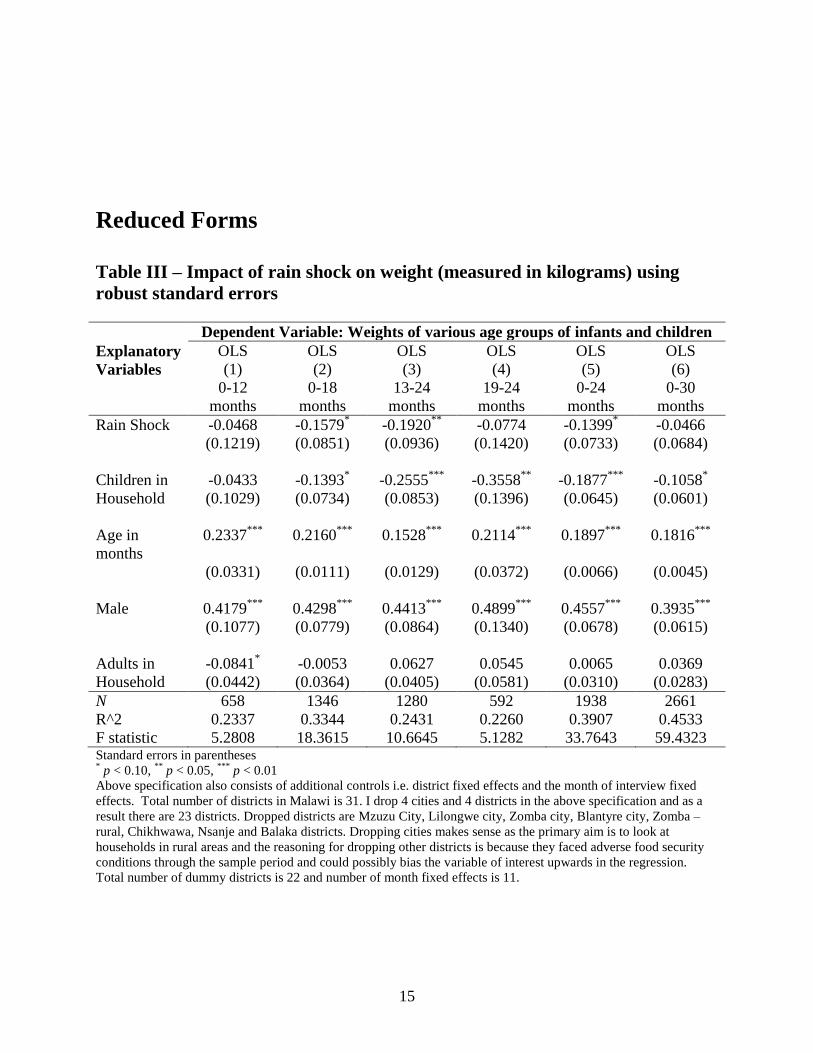
I estimate the reduced form equation where the child health measures are the

dependent variables in log terms and rain shock with the added controls and

dummies for districts and interview month to control for fixed effects as the

9

independent variables with robust standard errors. Tables III, IV and V in the

appendix give the estimation tables. For weight from Table III, I observe if

droughts occur in Malawi then for children up to 18 months old it reduces their

weight by 158 grams as compared to children from similar age group but who

experienced no drought. For children up to 18 months old mean weight is 9.36

kilograms and drought leads to about a 0.17 percent decrease in weight which is

significant. The same negative effect is observed for children aged 13 to 24

months and for children up to 24 months old. For these age groups drought

reduces weight by 192 and 140 grams i.e. 0.18 and 0.14 percent respectively.

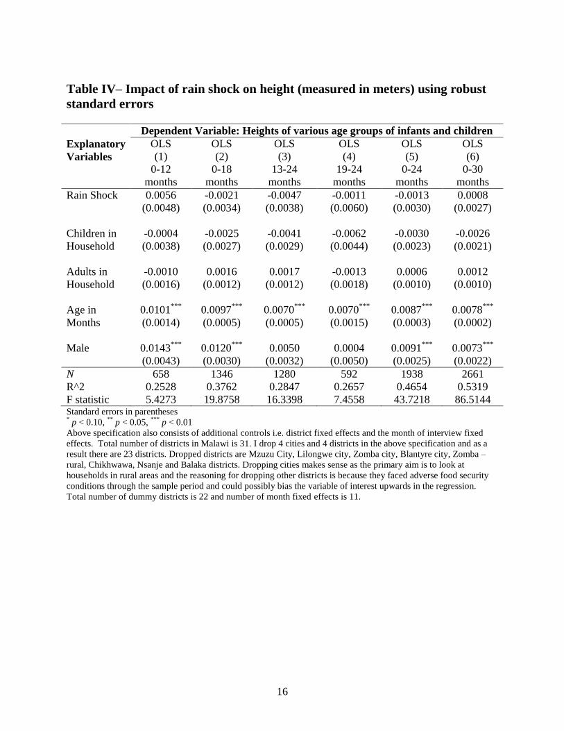
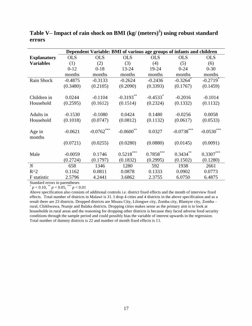
From Table IV, I observe for height, rain shocks have no impact and the

coefficients are tending to zero. From Table V, for BMI I observe BMI is negatively

affected by drought for ages up to 24 months and ages up to 30 months.

After going through the reduced forms and observing a relationship does exist

between drought and certain health outcomes for some age groups, following

Miguel’s income shock hypothesis, I utilize the channel of droughts leading to

income shocks leading to adverse health outcomes.

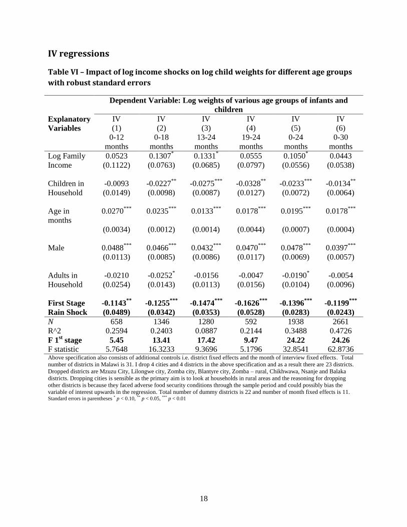
5.3 Instrument Variable Regressions

2SLS estimation procedure is used where droughts are considered as an

instrument for income shocks in explaining child health outcomes. The results for

weight are given in Table VI and Table VII in the appendix. For Table VI I consider

robust standard errors while for Table VII I consider cluster corrected standard

errors. In Table VI for age groups, up to 18 months, between 13 to 24 months

and up to 24 months the coefficients are significant. The first two coefficients

10

have similar coefficients and imply that a percent rise in income for the household

is associated with a 0.13 percent rise in weight for that age group. For children till

24 months a percent rise in income for the household is associated with a 0.10

percent rise in weight for that age group. Here weight is given in kilograms and

mean weight for children up to 18 months is 9.3602 kilograms and a resultant

change in weight in level terms is 121 grams. For children between 13 to 24

months this figure is about 136 grams and for children up to 24 months old it is 98

grams. These coefficients are very similar to the ones obtained in the reduced

form regression as given in Table III.

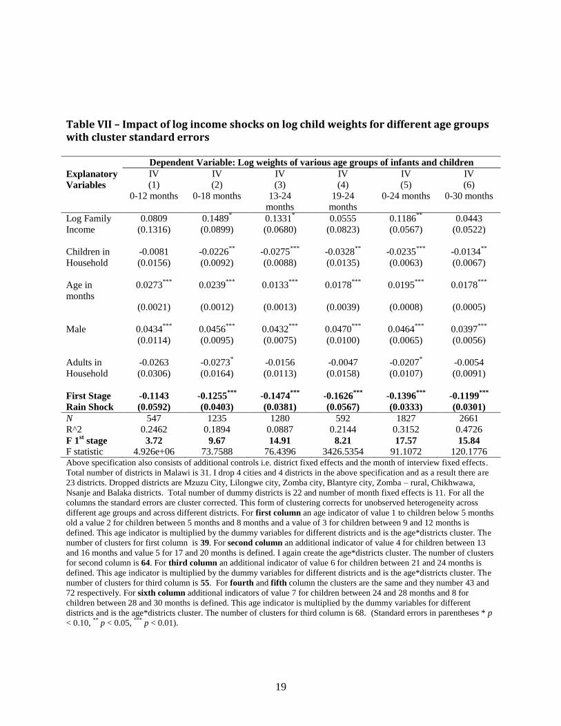
I also cluster correct the standard errors according to age and district where I

consider 4 month interval for children and multiply them by district dummies.

This methodology and clusters formed is explained in Table VII. Again the

coefficients obtained are very similar to the ones for Table VI and are significant

for the same age groups.

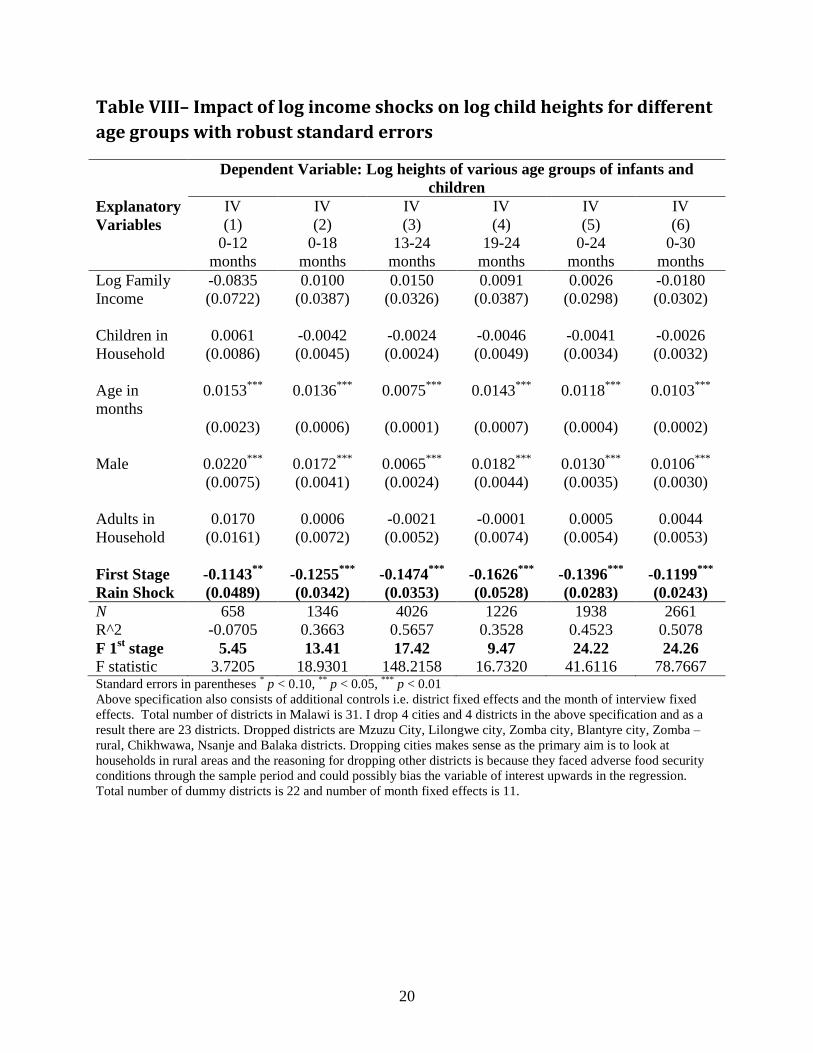
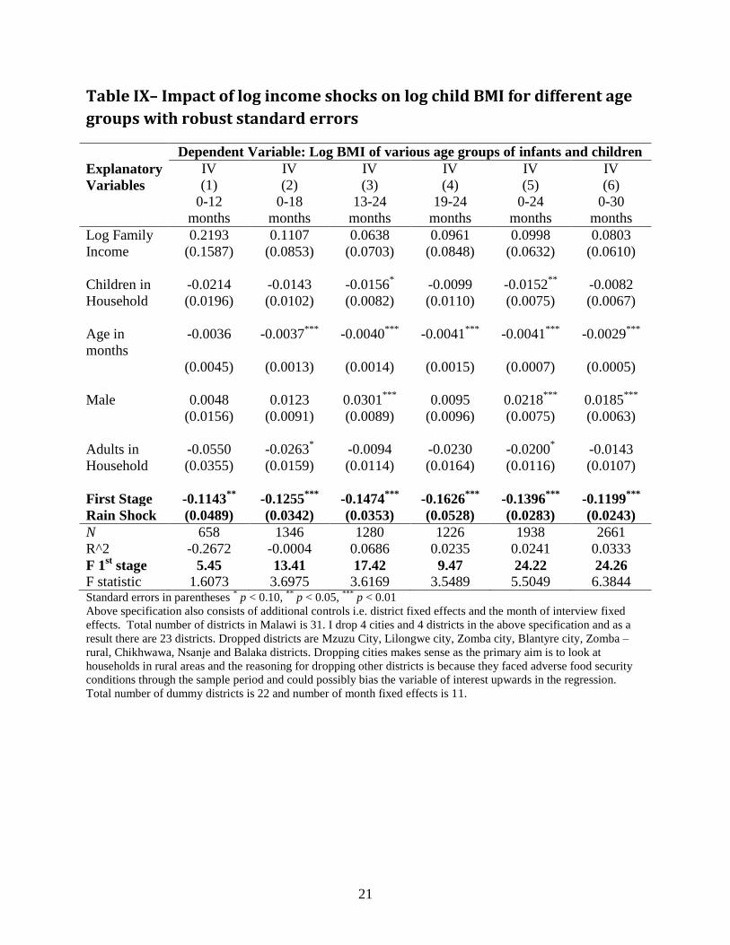
I run similar regressions for height and BMI and observe that none of the

coefficients are significant. The regression results are given in Table VIII and Table

IX in the appendix with robust standard errors.

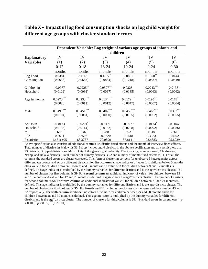
Next I consider log of food consumption as the independent variable as compared

to log of total consumption that was the proxy income measure. The regression

results are shown in Table X in the appendix. I observe for children aged between

13 to 24 months and for children till 24 months old the food consumption shock

variable is significant and a percent increase of food consumption increases by

0.16 percent and 0.11 percent for children 13 to 24 months old and for children

till 24 months old. These coefficients are slightly higher than the ones for total

11

consumption and makes sense because the channel of income shocks affecting

weight is through nutrition which is through food consumption. BMI and height

are insignificant and are not reported.

6. Conclusion

In this study I am able to estimate a relationship between income shocks and

child health outcomes for Malawi. I observe that adverse income shocks results in

adverse health outcome for children for the weight variable. This effect varies

among age groups subsections and is observed for children aged up to 18 months,

between 13 and 24 months and up to 24 months.

Further work for child health outcomes in response to adverse shocks can be

done using panel data. I would like to follow the outcome of the affected children

in these households over time and estimate whether their future outcomes will

be affected by this early life adversity. This can be done by utilizing the panel

component to the IHS3 survey where a subsample will be resampled in 2013.

I also have panel data for Uganda for 2009/2010 and 2010/2011 which can be

utilized to create a similar framework as for Malawi. What would be interesting to

check in this data is whether infant and child weight being similarly affected by

income shocks as in the case. If the age groups being affected are similar across

countries would be an interesting result.

12

References

[1] Hoddinott, John and Kinsey, Bill. 2001. Child Growth in the Time of Drought.

Oxford Bulletins of Economics and Statistics, 63, 4 (2001) 0305-9049

[2] Kudamatsu, Masayuki, Persson, Torsten and Strömberg, David. 2012. Weather

and Infant Mortality in Africa. CEPR Discussion paper 9222

[3] Miguel, Edward. Poverty and Witch Killing. 2005. Review of Economic Studies

72, 1153–1172

[4] Maccini, Sharon and Yang, Dean. 2009. Under the Weather: Health, Schooling,

and Economic Consequences of Early-Life Rainfall American Economic Review

2009, 99:3, 1006–1026

[5] Makoka, Donald. The Impact of Drought on Household Vulnerability: The Case

of Rural Malawi. 2008. Munich Personal RePEc Archive

[6] National Statistical Office Malawi . 2008. 2008 Population and Housing Census

[7] National Statistical Office Malawi . 2012. Integrated Household Survey 2010-

2011 Household Socio-Economic Characteristic Report

[8] Organization for Economic Co-operation and Development. 2007. African

Economic Outlook

13

Appendix

Table I - Summary Table

Variable Description Obs Mean Std. Dev. Min Max

Weight Weight of child in kilograms

(< 4 years) 4684 11.9 2.7 5.0 43.0

BMI Height of child in meters (< 4

years) 4684 17.2 3.2 7.4 57.6

Height BMI of child (< 4 years) 4684 0.8 0.1 0.4 1.2

Proxy Income

Total real annual consumption

per household in MWK

(1$=405.06MWK) 4684 223313.2 182871.5 24774.4 2456142.0

Food Consumption

Food, real annual consumption

in MWK 4684 138365.5 100678.2 7887.6 980378.3

Log weight Log Weight of child 4684 12.1 0.6 10.1 14.7

Log BMI Log BMI of child 4684 11.6 0.6 9.0 13.8

Log height Log Height of child 4684 2.4 0.2 1.6 3.8

Log proxy income

Log Total real annual

consumption per household 4684 2.8 0.2 2.0 4.1

Log Food Consumption

Log Food, real annual

consumption 4684 -0.2 0.1 -0.9 0.2

Rain Shock Drought/Irregular Rains 4684 0.4 0.5 0 1

Children in Household

Number of children in each household 4684

1.3 0.5 1 4

Total Adults Number of adults in each household 4684

2.6 1.2 1 13

Age in Months Age of each child in months 4684

27.6 12.1 2 48

Male Gender 4684 0.5 0.5 0 1

14

Table II - Base Regressions of Log Family Income and Log Food

Consumption on Log Child Health Measures with no controls

Dependent Variable: Log Child Health Measures

Explanatory OLS OLS OLS

Variable Log BMI Log Weight Log Height

Log Family 0.0134***

0.0283***

0.0075**

Income (0.0046) (0.0060) (0.0033)

N 3197 3197 3197

R^2 0.0026 0.0070 0.0016

F statistic 8.3721 22.4913 5.1712

Standard errors in parentheses

* p < 0.10,

** p < 0.05,

*** p < 0.01

Dependent Variable: Log Child Health Measures

Explanatory OLS OLS OLS

Variable Log BMI Log Weight Log Height

Log Food 0.0118**

0.0232***

0.0057*

Consumption (0.0046) (0.0059) (0.0033)

N 3197 3197 3197

R^2 0.0021 0.0047 0.0010

F statistic 6.5785 15.2478 3.0505

Standard errors in parentheses

* p < 0.10,

** p < 0.05,

*** p < 0.01

15

Reduced Forms

Table III – Impact of rain shock on weight (measured in kilograms) using

robust standard errors

Dependent Variable: Weights of various age groups of infants and children

Explanatory OLS OLS OLS OLS OLS OLS

Variables (1) (2) (3) (4) (5) (6)

0-12

months

0-18

months

13-24

months

19-24

months

0-24

months

0-30

months

Rain Shock -0.0468 -0.1579* -0.1920

** -0.0774 -0.1399

* -0.0466

(0.1219) (0.0851) (0.0936) (0.1420) (0.0733) (0.0684)

Children in -0.0433 -0.1393* -0.2555

*** -0.3558

** -0.1877

*** -0.1058

*

Household (0.1029) (0.0734) (0.0853) (0.1396) (0.0645) (0.0601)

Age in

months

0.2337***

0.2160***

0.1528***

0.2114***

0.1897***

0.1816***

(0.0331) (0.0111) (0.0129) (0.0372) (0.0066) (0.0045)

Male 0.4179***

0.4298***

0.4413***

0.4899***

0.4557***

0.3935***

(0.1077) (0.0779) (0.0864) (0.1340) (0.0678) (0.0615)

Adults in -0.0841* -0.0053 0.0627 0.0545 0.0065 0.0369

Household (0.0442) (0.0364) (0.0405) (0.0581) (0.0310) (0.0283)

N 658 1346 1280 592 1938 2661

R^2 0.2337 0.3344 0.2431 0.2260 0.3907 0.4533

F statistic 5.2808 18.3615 10.6645 5.1282 33.7643 59.4323 Standard errors in parentheses * p < 0.10,

** p < 0.05,

*** p < 0.01

Above specification also consists of additional controls i.e. district fixed effects and the month of interview fixed

effects. Total number of districts in Malawi is 31. I drop 4 cities and 4 districts in the above specification and as a

result there are 23 districts. Dropped districts are Mzuzu City, Lilongwe city, Zomba city, Blantyre city, Zomba –

rural, Chikhwawa, Nsanje and Balaka districts. Dropping cities makes sense as the primary aim is to look at

households in rural areas and the reasoning for dropping other districts is because they faced adverse food security

conditions through the sample period and could possibly bias the variable of interest upwards in the regression.

Total number of dummy districts is 22 and number of month fixed effects is 11.

16

Table IV– Impact of rain shock on height (measured in meters) using robust

standard errors

Dependent Variable: Heights of various age groups of infants and children


Variables (1) (2) (3) (4) (5) (6)

0-12

months

0-18

months

13-24

months

19-24

months

0-24

months

0-30

months

Rain Shock 0.0056 -0.0021 -0.0047 -0.0011 -0.0013 0.0008

(0.0048) (0.0034) (0.0038) (0.0060) (0.0030) (0.0027)

Children in -0.0004 -0.0025 -0.0041 -0.0062 -0.0030 -0.0026

Household (0.0038) (0.0027) (0.0029) (0.0044) (0.0023) (0.0021)

Adults in -0.0010 0.0016 0.0017 -0.0013 0.0006 0.0012

Household (0.0016) (0.0012) (0.0012) (0.0018) (0.0010) (0.0010)

Age in 0.0101***

0.0097***

0.0070***

0.0070***

0.0087***

0.0078***

Months (0.0014) (0.0005) (0.0005) (0.0015) (0.0003) (0.0002)

Male 0.0143***

0.0120***

0.0050 0.0004 0.0091***

0.0073***

(0.0043) (0.0030) (0.0032) (0.0050) (0.0025) (0.0022)

N 658 1346 1280 592 1938 2661

R^2 0.2528 0.3762 0.2847 0.2657 0.4654 0.5319


** p < 0.05,

*** p < 0.01








17

Table V– Impact of rain shock on BMI (kg/ (meters)2) using robust standard

errors

Dependent Variable: BMI of various age groups of infants and children


Variables (1) (2) (3) (4) (5) (6)

0-12

months

0-18

months

13-24

months

19-24

months

0-24

months

0-30

months

Rain Shock -0.4875 -0.3133 -0.2624 -0.2436 -0.3264* -0.2719

*

(0.3480) (0.2105) (0.2090) (0.3393) (0.1767) (0.1459)

Children in 0.0244 -0.1104 -0.3193**

-0.4533* -0.2016 -0.1014

Household (0.2595) (0.1612) (0.1514) (0.2324) (0.1332) (0.1132)

Adults in -0.1530 -0.1080 0.0424 0.1480 -0.0256 0.0058

Household (0.1018) (0.0747) (0.0812) (0.1132) (0.0617) (0.0533)

Age in

months

-0.0621 -0.0762***

-0.0600**

0.0327 -0.0738***

-0.0530***

(0.0721) (0.0255) (0.0280) (0.0880) (0.0145) (0.0091)

Male -0.0059 0.1746 0.5218***

0.7858***

0.3434**

0.3307***

(0.2724) (0.1797) (0.1832) (0.2995) (0.1502) (0.1280)

N 658 1346 1280 592 1938 2661

R^2 0.1162 0.0811 0.0878 0.1333 0.0902 0.0773


** p < 0.05,

*** p < 0.01








18

IV regressions

Table VI – Impact of log income shocks on log child weights for different age groups

with robust standard errors

Dependent Variable: Log weights of various age groups of infants and

children

Explanatory IV IV IV IV IV IV

Variables (1) (2) (3) (4) (5) (6)

0-12

months

0-18

months

13-24

months

19-24

months

0-24

months

0-30

months

Log Family 0.0523 0.1307* 0.1331

* 0.0555 0.1050

* 0.0443

Income (0.1122) (0.0763) (0.0685) (0.0797) (0.0556) (0.0538)

Children in -0.0093 -0.0227**

-0.0275***

-0.0328**

-0.0233***

-0.0134**

Household (0.0149) (0.0098) (0.0087) (0.0127) (0.0072) (0.0064)

Age in

months

0.0270***

0.0235***

0.0133***

0.0178***

0.0195***

0.0178***

(0.0034) (0.0012) (0.0014) (0.0044) (0.0007) (0.0004)

Male 0.0488***

0.0466***

0.0432***

0.0470***

0.0478***

0.0397***

(0.0113) (0.0085) (0.0086) (0.0117) (0.0069) (0.0057)

Adults in -0.0210 -0.0252* -0.0156 -0.0047 -0.0190

* -0.0054

Household (0.0254) (0.0143) (0.0113) (0.0156) (0.0104) (0.0096)

First Stage -0.1143**

-0.1255***

-0.1474***

-0.1626***

-0.1396***

-0.1199***

Rain Shock (0.0489) (0.0342) (0.0353) (0.0528) (0.0283) (0.0243)

N 658 1346 1280 592 1938 2661

R^2 0.2594 0.2403 0.0887 0.2144 0.3488 0.4726

F 1st stage 5.45 13.41 17.42 9.47 24.22 24.26

F statistic 5.7648 16.3233 9.3696 5.1796 32.8541 62.8736 Above specification also consists of additional controls i.e. district fixed effects and the month of interview fixed effects. Total

number of districts in Malawi is 31. I drop 4 cities and 4 districts in the above specification and as a result there are 23 districts.

Dropped districts are Mzuzu City, Lilongwe city, Zomba city, Blantyre city, Zomba – rural, Chikhwawa, Nsanje and Balaka

districts. Dropping cities is sensible as the primary aim is to look at households in rural areas and the reasoning for dropping

other districts is because they faced adverse food security conditions through the sample period and could possibly bias the

variable of interest upwards in the regression. Total number of dummy districts is 22 and number of month fixed effects is 11. Standard errors in parentheses * p < 0.10, ** p < 0.05, *** p < 0.01

19

Table VII – Impact of log income shocks on log child weights for different age groups with cluster standard errors Dependent Variable: Log weights of various age groups of infants and children


Variables (1) (2) (3) (4) (5) (6)

0-12 months 0-18 months 13-24

months

19-24

months

0-24 months 0-30 months

Log Family 0.0809 0.1489* 0.1331

* 0.0555 0.1186

** 0.0443

Income (0.1316) (0.0899) (0.0680) (0.0823) (0.0567) (0.0522)

Children in -0.0081 -0.0226**

-0.0275***

-0.0328**

-0.0235***

-0.0134**

Household (0.0156) (0.0092) (0.0088) (0.0135) (0.0063) (0.0067)

Age in

months

0.0273***

0.0239***

0.0133***

0.0178***

0.0195***

0.0178***

(0.0021) (0.0012) (0.0013) (0.0039) (0.0008) (0.0005)

Male 0.0434***

0.0456***

0.0432***

0.0470***

0.0464***

0.0397***

(0.0114) (0.0095) (0.0075) (0.0100) (0.0065) (0.0056)

Adults in -0.0263 -0.0273* -0.0156 -0.0047 -0.0207

* -0.0054

Household (0.0306) (0.0164) (0.0113) (0.0158) (0.0107) (0.0091)

First Stage -0.1143 -0.1255***

-0.1474***

-0.1626***

-0.1396***

-0.1199***

Rain Shock (0.0592) (0.0403) (0.0381) (0.0567) (0.0333) (0.0301)

N 547 1235 1280 592 1827 2661

R^2 0.2462 0.1894 0.0887 0.2144 0.3152 0.4726

F 1st stage 3.72 9.67 14.91 8.21 17.57 15.84

F statistic 4.926e+06 73.7588 76.4396 3426.5354 91.1072 120.1776 Above specification also consists of additional controls i.e. district fixed effects and the month of interview fixed effects.

Total number of districts in Malawi is 31. I drop 4 cities and 4 districts in the above specification and as a result there are

23 districts. Dropped districts are Mzuzu City, Lilongwe city, Zomba city, Blantyre city, Zomba – rural, Chikhwawa,

Nsanje and Balaka districts. Total number of dummy districts is 22 and number of month fixed effects is 11. For all the

columns the standard errors are cluster corrected. This form of clustering corrects for unobserved heterogeneity across

different age groups and across different districts. For first column an age indicator of value 1 to children below 5 months

old a value 2 for children between 5 months and 8 months and a value of 3 for children between 9 and 12 months is

defined. This age indicator is multiplied by the dummy variables for different districts and is the age*districts cluster. The

number of clusters for first column is 39. For second column an additional indicator of value 4 for children between 13

and 16 months and value 5 for 17 and 20 months is defined. I again create the age*districts cluster. The number of clusters

for second column is 64. For third column an additional indicator of value 6 for children between 21 and 24 months is


number of clusters for third column is 55. For fourth and fifth column the clusters are the same and they number 43 and

72 respectively. For sixth column additional indicators of value 7 for children between 24 and 28 months and 8 for

children between 28 and 30 months is defined. This age indicator is multiplied by the dummy variables for different

districts and is the age*districts cluster. The number of clusters for third column is 68. (Standard errors in parentheses * p

< 0.10, **

p < 0.05, ***

p < 0.01).

20

Table VIII– Impact of log income shocks on log child heights for different

age groups with robust standard errors

Dependent Variable: Log heights of various age groups of infants and

children


Variables (1) (2) (3) (4) (5) (6)

0-12

months

0-18

months

13-24

months

19-24

months

0-24

months

0-30

months

Log Family -0.0835 0.0100 0.0150 0.0091 0.0026 -0.0180

Income (0.0722) (0.0387) (0.0326) (0.0387) (0.0298) (0.0302)

Children in 0.0061 -0.0042 -0.0024 -0.0046 -0.0041 -0.0026

Household (0.0086) (0.0045) (0.0024) (0.0049) (0.0034) (0.0032)

Age in

months

0.0153***

0.0136***

0.0075***

0.0143***

0.0118***

0.0103***

(0.0023) (0.0006) (0.0001) (0.0007) (0.0004) (0.0002)

Male 0.0220***

0.0172***

0.0065***

0.0182***

0.0130***

0.0106***

(0.0075) (0.0041) (0.0024) (0.0044) (0.0035) (0.0030)

Adults in 0.0170 0.0006 -0.0021 -0.0001 0.0005 0.0044

Household (0.0161) (0.0072) (0.0052) (0.0074) (0.0054) (0.0053)


-0.1255***

-0.1474***

-0.1626***

-0.1396***

-0.1199***

Rain Shock (0.0489) (0.0342) (0.0353) (0.0528) (0.0283) (0.0243)

N 658 1346 4026 1226 1938 2661

R^2 -0.0705 0.3663 0.5657 0.3528 0.4523 0.5078

F 1st stage 5.45 13.41 17.42 9.47 24.22 24.26

F statistic 3.7205 18.9301 148.2158 16.7320 41.6116 78.7667 Standard errors in parentheses

* p < 0.10,

** p < 0.05,

*** p < 0.01








21

Table IX– Impact of log income shocks on log child BMI for different age

groups with robust standard errors

Dependent Variable: Log BMI of various age groups of infants and children


Variables (1) (2) (3) (4) (5) (6)

0-12

months

0-18

months

13-24

months

19-24

months

0-24

months

0-30

months

Log Family 0.2193 0.1107 0.0638 0.0961 0.0998 0.0803

Income (0.1587) (0.0853) (0.0703) (0.0848) (0.0632) (0.0610)

Children in -0.0214 -0.0143 -0.0156* -0.0099 -0.0152

** -0.0082

Household (0.0196) (0.0102) (0.0082) (0.0110) (0.0075) (0.0067)

Age in

months

-0.0036 -0.0037***

-0.0040***

-0.0041***

-0.0041***

-0.0029***

(0.0045) (0.0013) (0.0014) (0.0015) (0.0007) (0.0005)

Male 0.0048 0.0123 0.0301***

0.0095 0.0218***

0.0185***

(0.0156) (0.0091) (0.0089) (0.0096) (0.0075) (0.0063)

Adults in -0.0550 -0.0263* -0.0094 -0.0230 -0.0200

* -0.0143

Household (0.0355) (0.0159) (0.0114) (0.0164) (0.0116) (0.0107)


-0.1255***

-0.1474***

-0.1626***

-0.1396***

-0.1199***

Rain Shock (0.0489) (0.0342) (0.0353) (0.0528) (0.0283) (0.0243)

N 658 1346 1280 1226 1938 2661

R^2 -0.2672 -0.0004 0.0686 0.0235 0.0241 0.0333

F 1st stage 5.45 13.41 17.42 9.47 24.22 24.26

F statistic 1.6073 3.6975 3.6169 3.5489 5.5049 6.3844 Standard errors in parentheses

* p < 0.10,

** p < 0.05,

*** p < 0.01








22

Table X – Impact of log food consumption shocks on log child weight for

different age groups with cluster standard errors

Dependent Variable: Log weight of various age groups of infants and

children


Variables (1) (2) (3) (4) (5) (6)

0-12

months

0-18

months

13-24

months

19-24

months

0-24

months

0-30

months Log Food 0.0381 0.1118 0.1577

* 0.0801 0.1058

** 0.0444

Consumption (0.0638) (0.0687) (0.0884) (0.1218) (0.0537) (0.0519)

Children in -0.0077 -0.0225**

-0.0307***

-0.0328**

-0.0243***

-0.0138**

Household (0.0122) (0.0092) (0.0097) (0.0135) (0.0063) (0.0062)

Age in months 0.0273***

0.0233***

0.0134***

0.0172***

0.0195***

0.0178***

(0.0020) (0.0011) (0.0012) (0.0047) (0.0007) (0.0004)

Male 0.0491***

0.0451***

0.0402***

0.0455***

0.0463***

0.0393***

(0.0104) (0.0081) (0.0080) (0.0105) (0.0062) (0.0055)

Adults in -0.0173 -0.0201* -0.0171 -0.0079 -0.0174

* -0.0047

Household (0.0133) (0.0114) (0.0132) (0.0208) (0.0092) (0.0086)

N 658 1346 1280 592 1938 2661

R^2 0.2611 0.2592 -0.0320 0.1618 0.3323 0.4692

F statistic 1.461e+05 68.3767 70.0890 87.8111 92.4383 95.6929

Above specification also consists of additional controls i.e. district fixed effects and the month of interview fixed effects.

Total number of districts in Malawi is 31. I drop 4 cities and 4 districts in the above specification and as a result there are

23 districts. Dropped districts are Mzuzu City, Lilongwe city, Zomba city, Blantyre city, Zomba – rural, Chikhwawa,

Nsanje and Balaka districts. Total number of dummy districts is 22 and number of month fixed effects is 11. For all the

columns the standard errors are cluster corrected. This form of clustering corrects for unobserved heterogeneity across

different age groups and across different districts. For first column an age indicator of value 1 to children below 5 months

old a value 2 for children between 5 months and 8 months and a value of 3 for children between 9 and 12 months is


number of clusters for first column is 39. For second column an additional indicator of value 4 for children between 13

and 16 months and value 5 for 17 and 20 months is defined. I again create the age*districts cluster. The number of clusters

for second column is 64. For third column an additional indicator of value 6 for children between 21 and 24 months is


number of clusters for third column is 55. For fourth and fifth column the clusters are the same and they number 43 and

72 respectively. For sixth column additional indicators of value 7 for children between 24 and 28 months and 8 for

children between 28 and 30 months is defined. This age indicator is multiplied by the dummy variables for different

districts and is the age*districts cluster. The number of clusters for third column is 68. (Standard errors in parentheses * p

< 0.10, **

p < 0.05, ***

p < 0.01).

Impact of Income Shocks on child health outcomes in Malawi

Documents

Transcript of Impact of Income Shocks on child health outcomes in Malawi