1

Stealing to Survive? Crime and Income Shocks in 19th

Century France♣♣♣♣

Vincent Bignon*

Banque de France

Eve Caroli◊ Paris Dauphine University, LEDa-LEGOS, Paris School of Economics and IZA

Roberto Galbiati∇

CNRS-OSC, Sciences Po Paris

Keywords: crime, income shock, phylloxera, 19th century France. JEL code: K42, N33, R11

♣ We wish to thank Andrea Bassanini, Jean-Pierre Dormois, Francesco Drago, Cecilia Garcia-Peñalosa, Elise Huillery, Francis Kramarz, Giovanni Mastrobuoni, Naci Mocan, Tommy Murphy, Tommaso Nannicini, Emily Owens, Jens Prufer, Michael Visser, Ben Vollard and participants to seminars at University Bocconi, the Paris School of Economics, Sciences Po, Université Paris Dauphine, CentER at Tilburg University and at the Royal Economic Society conference in Cambridge for useful comments and discussions. Charlotte Coutand and Clement Malgouyres provided excellent research assistance. We also thank Pierre-Emmanuel Couralet and Fabien Gaveau who proved crucial in helping us with some of the data. We are grateful to Gilles Postel-Vinay for sharing with us his data on wine and phylloxera and for insightful comments and suggestions. The views expressed in the paper are those of the authors and do not necessarily reflect those of Banque de France or the Eurosystem. The usual disclaimer applies. * Banque de France. Pomone- DGEI – DEMFI (041-1422) ; 31, rue des Petits Champs. 75049 Paris Cedex 01 France. Email : vincent.bignon@banque-france.fr ◊ LEDa-LEGOS, Université Paris Dauphine, Place du Maréchal de Lattre de Tassigny, 75775 Paris Cedex 16. France. Email: eve.caroli@dauphine.fr ∇ Sciences Po. 28 Rue des Saints-Pères 75007 Paris. France. Email: galbiatir@gmail.com

2

Abstract

Using local administrative data from 1826 to 1936, we document the evolution of crime rates

in 19th century France and we estimate the impact of a negative income shock on crime. Our

identification strategy exploits the phylloxera crisis. Between 1863 and 1890, phylloxera

destroyed about 40% of French vineyards. We use the geographical variation in the timing of

this shock to identify its impact on property and violent crime rates, as well as minor offences.

Our estimates suggest that the phylloxera crisis caused a substantial increase in property crime

rates and a significant decrease in violent crimes.

3

1. Introduction

Economic theory and casual observation both suggest that bad economic conditions,

economic crises and poverty may favour criminal activity as they alter the opportunity costs

to engage into crime. At the same time, higher crime rates are likely to have a negative impact

on economic growth as the prevalence of crime in an area discourages business. Thus, crime

and bad economic conditions may reinforce each other so that countries may be stuck in a

high crime - low growth equilibrium. This might be particularly true in developing countries

where, in the absence of social safety net, people falling into poverty during an economic

crisis might be pushed to commit crime to survive. Despite intuitive this relation is far from

easy to document due to standard endogeneity problems. Moreover, analysing the issue

requires reliable data on crime records, matched with information on relevant economic

variables and both these variables are not easily available for developing countries for a

sufficient number of years. In order to single out the causal impact of negative shocks to the

economy on crime rates, ideally we would like to observe a comparable set of developing

countries or administrative units within a country over a long period of time and we would

like to treat randomly some of them inducing negative economic shocks. On top of such an

ideal experiment we would like to have reliable data on crime rates with both time and spatial

variation. In this paper, we claim that 19th century France provides such an ideal setting.

We resort to uniquely rich data on criminal records collected between 1826 and 1936 by the

French Ministry of Justice at the département level (a geographical area roughly equal in size

to a US county). These data are unique and represent to the best of our knowledge the oldest

national official administrative crime record exploited by researchers up to today. To identify

the impact of a negative economic shock on crime, we take advantage of the phylloxera crisis

that burst in France in the second half of the 19th century. The phylloxera (an aphid which

attacks vines' roots) destroyed about 40 per cent of vines in France, thus inducing a large

4

productivity shock in an economy still largely dependent on agricultural production1.

According to historical research, this turned into a major income shock for a number of

reasons. First, the decrease in wine production was not matched, by far, by an equivalent

increase in wine prices. Second, the reduction in wine-generated income did not trigger a

substantial substitution of wine for other agricultural products. Eventually, in some

départements, the crisis was so strong as to induce a partial collapse of the local credit system

(Postel Vinay, 1989), thus preventing any smoothing of the crisis. In the absence of welfare

state, a large share of the population suffered a major income drop.

The phylloxera crisis started in 1863 when the aphid appeared in Southern France and ended

in the 1890s when vineyards were replanted with hybrid American vines which were resistant

to the insect. As phylloxera affected the different départements in different years, we exploit

spatial variation in the timing of the shock to identify its effect on crime rates. The massive

negative shock to the French economy induced by the phylloxera attack is indeed an ideal

natural experiment that helps solving the major identification problems related to reverse

causality and confounding factors. To the best of our knowledge, the only article exploiting

the source of exogenous variation in income induced by phylloxera is Banerjee et al. (2010)

who estimate the effect of the shock in utero and during early childhood on future health

conditions.

We use a similar research design to identify how negative income shocks affected local crime

rates in 19th century France. The very rich data collected by the French administration starting

from 1826 allow us to identify the impact of the crisis on violent and property crimes, as well

as on minor offences. This exercise is unique from a historical perspective since comparable

datasets were collected only starting in the 20th century in other countries (e.g. the Uniform

crime report in the USA starts being compiled in the 1930s) or for a shorter period of time in 1 Wine represented on average 17% of agricultural production.

5

some German states like Bavaria and Prussia (see Mehlum et al., 2006 and Traxler and

Burhop, 2010).

Our results show that the phylloxera crisis caused a strong increase in property crimes and a

significant decrease in violent crimes. In particular, the fall in wine production and hence in

agricultural income induced by the phylloxera attack caused a strong increase in thefts and a

reduction in homicides.

This paper contributes to the literature on the effects of negative economic conditions on

crime in a historical perspective by covering 87 French départements over 1826-1936.2

Besides being informative for the economics of crime and being one of the very first exercises

of this kind in economic history, this paper also contributes to the literature in development

economics to the extent that the economic and demographic structures of 19th century France

were very similar to those of a developing country (Banerjee et al 2010).

To the best of our knowledge, only a couple of papers resort to historical data to study the

impact of changing economic conditions on crime. Mehlum et al. (2006) estimate the impact

of poverty on crime in 19th century Bavaria. The authors use rainfall as an instrumental

variable for rye prices and show that an increase in rye prices following bad weather

conditions induces an increase in property crimes and leads to significantly fewer violent

crimes. Traxler and Burhop (2010) replicate this exercise for Prussia and find similar results.

With respect to Mehlum et al. (2006), it is worth noting that despite we cover a similar

historical period, our research design has a number of advantages. We have observations for

both our independent and dependent variables for each of the 87 French départements over

the whole period of analysis. In contrast, Mehlum et al. (2006) use data on crime rates in

seven Bavarian regions while they only have one single series of rainfall and rye price data

2 We exclude Meurthe, Meurthe-et-Moselle as well as Moselle from our dataset. Moreover, for 5 of the 87 départements we have data for a shorter period of time – see Data Appendix.

6

for the whole of Bavaria. Moreover, while rainfall potentially affects both economic

conditions and the probability of apprehension of criminals – since the cost of searching for

criminals may be higher if weather conditions are bad –, the phylloxera crisis affects incomes

while leaving unaltered the cost of crime fighting and hence the probability of apprehension.

A few papers tackle the impact of a negative income shock on criminal activity in developing

countries. Miguel (2005) uses survey data on contemporary rural Tanzania to show that the

killing of “witches” (i.e. old women) increases in times of extreme weather events leading to

floods and droughts. Fafchamps and Minten (2006) exploit an exogenous cut in fuel supply in

rural Madagascar following a disputed presidential election to identify the effects of a massive

increase in poverty and transport costs. Using original survey data collected in 2002 they find

that crop thefts increase with transitory poverty. Theft thus appears to be used by some of the

rural poor as a risk coping strategy.

Our paper relates more indirectly to the recent literature on unemployment and crime in

contemporary developed countries. These studies using panel data at the state or regional

level (Raphael and Winter-Ebmer, 2001; Gould et al., 2002; Oster and Agell, 2007; Lin, 2008;

Buonanno and Montolio, 2008; Fougère et al., 2009; Mocan and Bali, 2010) reach a

consensus that increasing unemployment contributes to raise property crimes (although the

magnitude is not large) and does not significantly affect violent crimes. Our paper also

investigates the impact of worsening economic conditions on crimes rates, but in a much

longer historical perspective. It also relates, to some extent, to the literature on the effects of

the business cycle on crime since the phylloxera crisis constitutes a strong negative shock to

the French economy. Consistent with our findings, this literature finds that trends in property

crimes in the USA and France are countercyclical (Cook and Zarkin, 1985 and Lagrange,

2003).

7

While these papers focus on the effects of poverty and income shocks, other papers

investigate the effect of structural poverty and inequality on crime. Resorting to cross-country

comparisons, Fajnzylber et al. (2002) show that differences in crime rates are related to

growth and poverty.

The paper develops as follows. Section 2 provides some background information about the

phylloxera pest and some conceptual background. Section 3 presents our empirical strategy.

Section 4 describes the data sources and the main trends in crime rates and phylloxera

diffusion in 19th century France. Section 5 presents the results and Section 6 provides some

conclusions.

2.Historical and Theoretical Background

2.1.Phylloxera and income shock

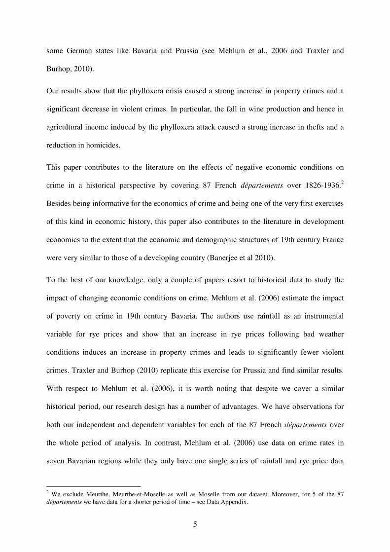
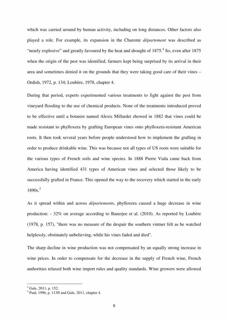
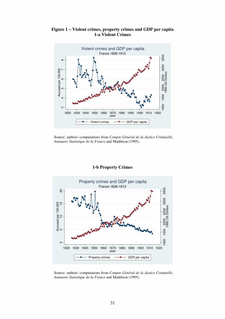
Over the 19th century, France experienced modest but constant economic growth with GDP

rising from $1,218 in 1820 to $3,452 in 1913.3 While income per capita thus increased by

about 200%, crime rates decreased quite sharply. Violent crimes declined from 6 per 100,000

inhabitants in 1826 to 4.3 in 1913, while property crimes precipitated from about 15.9 to 3.4

per 100,000 over the same period. One candidate explanation for the correlation evidenced by

Figures 1a-b between declining crime rates and increasing GDP per capita is, of course, the

existence of a negative relationship between income and crime – Becker (1968).

At the beginning of the 19th century, France was still a developing country. Agriculture still

represented a major source of income for many households. The share of agricultural

production and extractive industry in GDP amounted to 38.5% in 1830, decreased to 33% in

1850 and was still as high as 28% in 1890 (Craft, 1984, p. 54). This made France much more

3 1990 Geary-Khamis dollars (see Maddison, 1995).

8

dependent on agriculture than the United-Kingdom, for example, where the corresponding

shares were respectively 24.9% in 1840 and 13.4% in 1890 (Craft, 1984, p. 53). Wine

production represented a large part of the value of agricultural production. In 1862, the year

before phylloxera was first spotted in France, wine production amounted to about one-sixth of

the value of agricultural production thus representing the second most important product after

wheat. Any disease affecting French vineyards was therefore likely to represent a major shock

to a mostly rural economy. Phylloxera turned out to be such a shock.

"Phylloxera vastatrix" is a near-microscopic aphid that hangs on the roots of vines and sucks

the sap. It originally lived in North America and did not reach Europe in the era of sailing

ships since the journey took so long that upon arrival either the vine cuttings or the aphid on

them had died. The steam power provided the greater speed necessary for the insect to survive

the journey. Although it was harmless to grape vines in its original ecology, it proved

devastator to European species, causing their death in a very short while (Simpson, 2011,

p.36). French vineyards started to be affected in 1863 but it was not before 1868 that scientists

identified its presence on dead roots in the Gard département. Until 1875, there was a fierce

scientific debate as to the responsibility of phylloxera in vines death. Some scientists argued

that it was the cause of the death whereas most of them claimed that it was a consequence of

it: vines were dying because wine growers would not take good care of them and phylloxera

was developing on dead vines (Pouget, 1990 and Gale, 2011).

By the end of the 1860s, the aphid affected most départements in the Southeast of the country

(Bouches du Rhône) and in the Bordeaux region. From the Southeast, it moved northward and

from the Bordeaux region it moved northwest. The insect progressively expanded across

départements and by the end of the 1870s it had affected all wine producing départements in

Southern France. Its expansion path was very difficult to predict since phylloxera spread

either because it was carried by the wind or because it was hanging on an object or a plant

9

which was carried around by human activity, including on long distances. Other factors also

played a role. For example, its expansion in the Charente département was described as

“nearly explosive” and greatly favoured by the heat and drought of 1875.4 So, even after 1875

when the origin of the pest was identified, farmers kept being surprised by its arrival in their

area and sometimes denied it on the grounds that they were taking good care of their vines –

Ordish, 1972, p. 134; Loubère, 1978, chapter 4.

During that period, experts experimented various treatments to fight against the pest from

vineyard flooding to the use of chemical products. None of the treatments introduced proved

to be effective until a botanist named Alexis Millardet showed in 1882 that vines could be

made resistant to phylloxera by grafting European vines onto phylloxera-resistant American

roots. It then took several years before people understood how to implement the grafting in

order to produce drinkable wine. This was because not all types of US roots were suitable for

the various types of French soils and wine species. In 1888 Pierre Viala came back from

America having identified 431 types of American vines and selected those likely to be

successfully grafted in France. This opened the way to the recovery which started in the early

1890s.5

As it spread within and across départements, phylloxera caused a huge decrease in wine

production: - 32% on average according to Banerjee et al. (2010). As reported by Loubère

(1978, p. 157), "there was no measure of the despair the southern vintner felt as he watched

helplessly, obstinately unbelieving, while his vines faded and died".

The sharp decline in wine production was not compensated by an equally strong increase in

wine prices. In order to compensate for the decrease in the supply of French wine, French

authorities relaxed both wine import rules and quality standards. Wine growers were allowed

4 Gale, 2011, p. 152. 5 Paul, 1996, p. 113ff and Gale, 2011, chapter 4.

10

to sell "piquettes" or "second or third wine" – made by mixing press cakes with water,

pressing it, adding sugar to the run and fermenting. They were also allowed to produce raisin

wines, a beverage made out by soaking imported dried raisins and drawing off the liquid until

the exhaustion of all of its sugar (Loubère, 1978, p. 166). According to Ordish (1972, tables 9-

11), the sum of imports, piquettes and raisin wine represented 58.6% of domestic wine

production in 1889 and 61.5% in 1890 as compared to less than 0.5% in the 1860s.6 This large

inflow of imports and wine substitutes together with the decrease in average wine quality kept

the price of wine from increasing at the same pace as the decline in French production

(Ordish, 1972; Banerjee et al, 2010).

This generated a major income shock. Contemporary estimates made by A. Lalande suggest

that phylloxera cost France twice as much as the war indemnity paid to the Germans in 1870

which amounted to 25% of one-year GDP (see Occhino et al, 2008 and Ordish, 1972). More

recently, Pierre Galet estimated that the cost could have been as high as 15 billion francs, i.e.

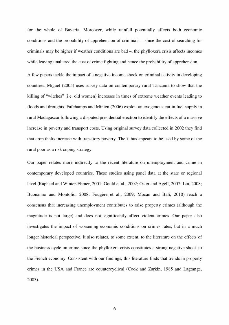
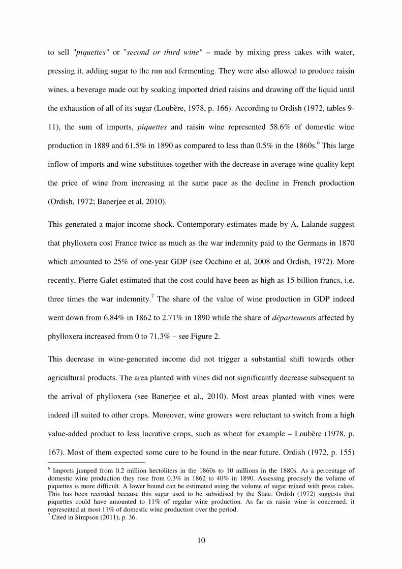
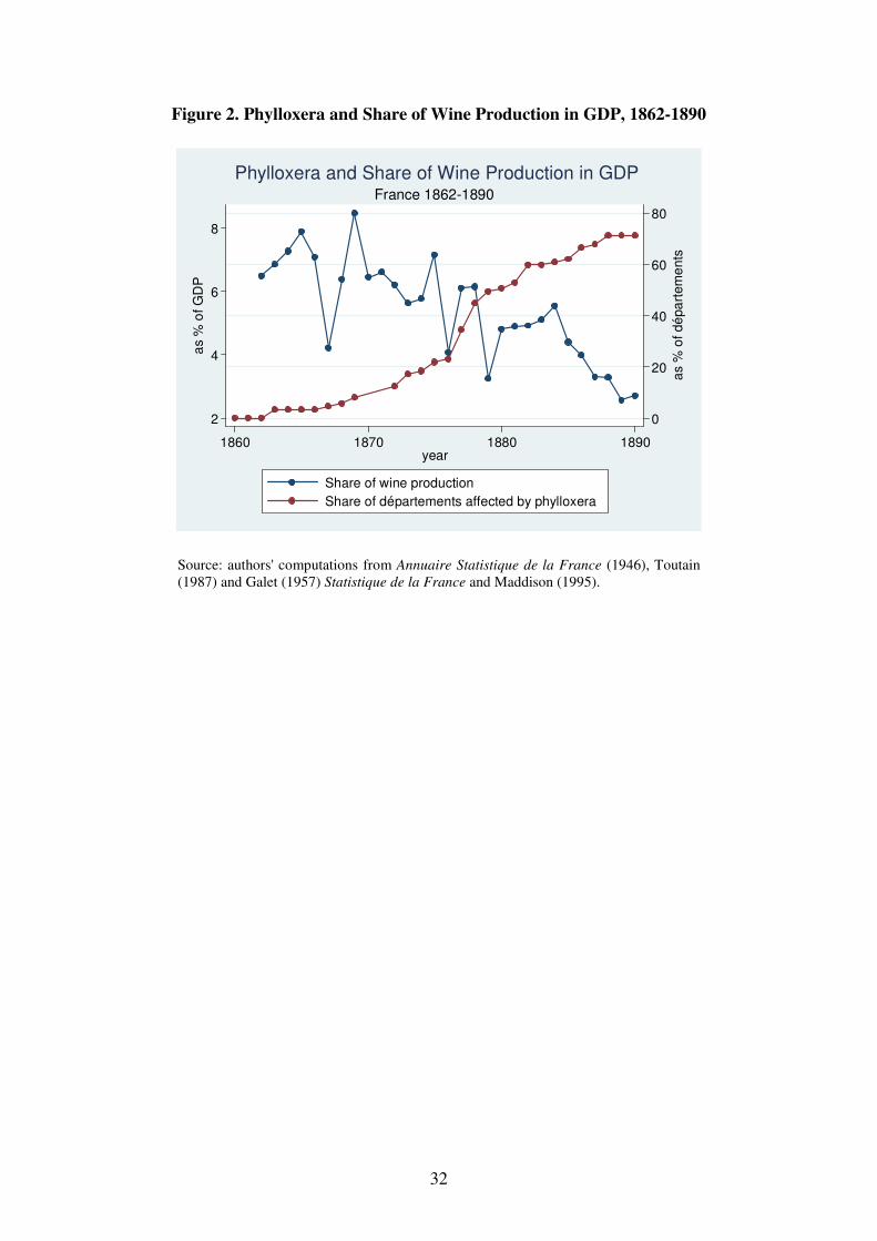
three times the war indemnity.7 The share of the value of wine production in GDP indeed

went down from 6.84% in 1862 to 2.71% in 1890 while the share of départements affected by

phylloxera increased from 0 to 71.3% – see Figure 2.

This decrease in wine-generated income did not trigger a substantial shift towards other

agricultural products. The area planted with vines did not significantly decrease subsequent to

the arrival of phylloxera (see Banerjee et al., 2010). Most areas planted with vines were

indeed ill suited to other crops. Moreover, wine growers were reluctant to switch from a high

value-added product to less lucrative crops, such as wheat for example – Loubère (1978, p.

167). Most of them expected some cure to be found in the near future. Ordish (1972, p. 155) 6 Imports jumped from 0.2 million hectoliters in the 1860s to 10 millions in the 1880s. As a percentage of domestic wine production they rose from 0.3% in 1862 to 40% in 1890. Assessing precisely the volume of piquettes is more difficult. A lower bound can be estimated using the volume of sugar mixed with press cakes. This has been recorded because this sugar used to be subsidised by the State. Ordish (1972) suggests that piquettes could have amounted to 11% of regular wine production. As far as raisin wine is concerned, it represented at most 11% of domestic wine production over the period. 7 Cited in Simpson (2011), p. 36.

11

even argues that "there was a mystique attached to wine growing felt by the majority of small

growers who found it difficult to envisage any other way of life".

Given the size of the income shock in wine producing départements, the credit system itself

partly collapsed thus preventing farmers from relying on borrowing to smooth out the crisis

(Postel-Vinay, 1989). Central and local governments would not provide any financial help to

compensate for the loss of income. Moreover, the only institutions in charge of poor relief, the

so-called bureaux de bienfaisance, were charities organised on a local community basis which

found themselves in great difficulty because of the crisis. The British consul at Bordeaux

noticed in 1886 that "the number, more especially of the smaller class of proprietors on

Medoc, in Sauterne and other départements of the Gironde who have been utterly ruined is

considerable".8 Similarly, Arambourou (1958) summarises: "For many peasants, ruin was

complete; for all of them the financial difficulty was considerable".

2.2 Income shock and crime

According to the standard economic model of crime (Becker, 1968), individuals choose

between criminal and legal activities on the basis of the expected utility of each. Consistently,

evidence from contemporary data have shown that crime rates respond to falls in the wages of

unskilled workers causing a variation in the relative utility to engage into legal activities

(Machin and Meghir, 2004). In a similar way, we expect the income shock brought about by

phylloxera to have affected the expected utility from illegal activities, and hence crime rates,

in several respects.

First it decreased the quantity and quality of legitimate earnings opportunities, thereby

reducing the opportunity cost of illegal behaviour. At the same time, phylloxera also reduced

the quality and quantity of wine production potentially targeted by criminals, thereby reducing

the gains from crime. So phylloxera has modified the relative gains from legal versus illegal 8 Cited in Ordish, 1972, p. 146.

12

activities in a potentially ambiguous way. The rest of the paper aims at assessing the causal

impact of the income shock generated by phylloxera on crime rates.

However the decision to engage in criminal activity does not only depend on the relative gains

from criminal and non-criminal activities. It also depends on the probability of apprehension

and on the severity of court sentences. Both may have been affected by the income shock

generated by phylloxera.

Local tax revenues may have decreased following the fall in income, triggering a reduction in

the number of police forces and/or in their endowments. This may, in turn, have reduced the

probability of apprehending criminals. However, such a reduction in the number of police

forces is not very likely to have taken place. The number and availability of police forces was

indeed mainly determined at the national level so that it was not very sensitive to local

economic conditions. Nonetheless, we control for the local presence of police forces in some

specifications in order to make sure that this does not bias our results. These are not our

preferred estimates to the extent that police forces are, of course, likely to be endogenous.

The severity of court sentences may also have decreased if judges became more lenient

because they were conscious that making a living out of legal income opportunities had

become more difficult.9 In order to make sure that our results on crime rates are not driven by

a greater leniency of judges in hard times, we run some robustness checks in which we check

that phylloxera did not significantly affect conviction rates.

3. Empirical framework

Our identification strategy relies on the fact that phylloxera affected different départements in

different years. The exogeneity of the variation of the phylloxera spread with respect to crime

9 Ichino et al. (2003), for instance, show that Italian labour judges are more likely to decide in favour of workers whenever local unemployment is higher.

13

is central to our strategy. Ideally we would regress crime rates on département-level income,

instrumenting the latter with an indicator of phylloxera – as defined in section 4 – in order to

identify the effect of the induced income shock on both property and violent crime rates as

well as minor offences. However income data do not exist at the département level for 19th

century France.

As an alternative strategy we estimate the reduced form relation between phylloxera and

crime rates for the 87 French départements for the period from 1826 to 1936 – except war

years.

We first check that phylloxera did actually reduce wine production, running the following

regression of the log of wine production on a phylloxera indicator:

where Wineij denotes wine production in département i at year j, pij is our phylloxera

indicator, tj and di represent year and département fixed effects respectively, while sij is a

département time-specific trend and εij is an error term. In all specifications, standard errors

are clustered at the département level.

As a second step, we assess the impact of phylloxera on crime rates by estimating the

following equation:

where Cij is the crime rate in département i during year j. Depending on the specification Cij

represents either property or violent crimes, minor offences or some sub-category of crimes

such as theft and murder.

Since the impact of the crisis might have been stronger in areas highly dependent on wine

production, we also check whether the impact of phylloxera on crime rates varies according to

the importance of wine-growing in the department in 1862, i.e. prior to the arrival of

phylloxera. The equation we estimate is then:

14

where denotes the importance of wine-growing in département i as of 1862.

In some specifications we add a set of département-level socio-demographic controls or a

measure of the importance of police forces (Xij). The corresponding equation is:

Finally we check that phylloxera did not affect the leniency of courts by regressing conviction

rates CRij on our phylloxera indicator:

4. Data

4.1 Crime and police forces

Since the very beginning of the 19th century, the French judicial system was highly

centralized. France was a Roman-law country where the Napoleonic codes were the basis of

criminal and civil law (Carbasse, 2000). Starting in 1826, the French Ministry of Justice

published a statistical yearbook entitled the Compte Général de la Justice Criminelle. It was

based on reporting by local court public prosecutors and clerks. We hand-collected data from

this source.

The Compte Général was one of the most continuous and reliable sources in France at that

time. It has been used as a model to set up criminal statistical records in several countries (see

Perrot and Robert, 1989). Since its first publication, the Compte was assigned a double role. It

was a management tool that was designed to help the government assess the working of the

law and the effects of legal reforms. But, beyond policy makers, it was also supposed to

provide information to moralists and thinkers. As such it contributed to the birth of

criminology. Despite the Compte was published yearly until 1982, we only collected data for

the period from 1826 to 1936. As underlined by Perrot and Robert (1989) the quality of the

15

data indeed declined after the 1930s, in particular due to the decrease in the funding awarded

to the judiciary system to collect statistical information.

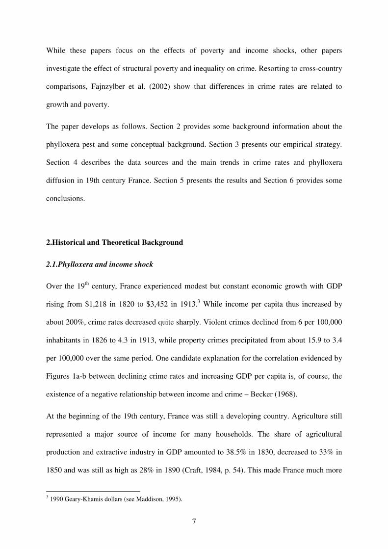
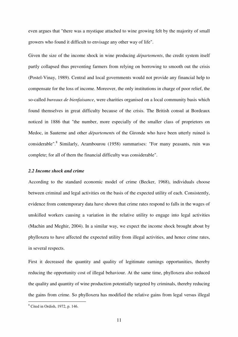
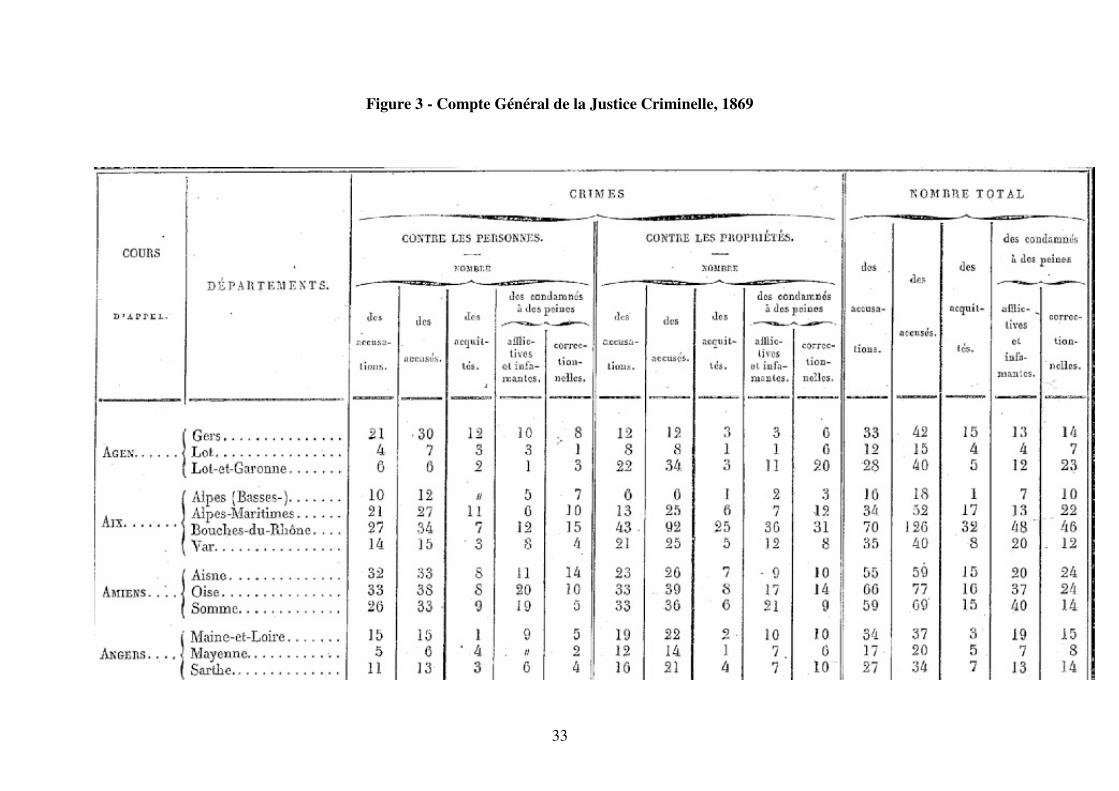
The Compte provides detailed information on the number of people charged and acquitted of

violent crimes, property crimes and minor offences in each département every year (see

Figure 3 for crimes – a similar table is available for minor offences). Violent crimes include

homicides, sexual assaults, injuries, violence against children, abortion, plotting, rebellion and

false witnesses. Property crimes encompass thefts, counterfeiting, corruption, destruction,

fires and pillaging. We also have data on the number of people accused of a number of more

precisely defined crimes such as: homicides, thefts in churches, on country roads, domestic

thefts and other thefts. Using the population provided by the Census10 for each département,

we compute yearly crime rates defined as the ratio of the number of people accused to the

population, broken down by type of crimes and offences, in each département over 1826-

1936. Given the poor quality of population data during war years, we drop years 1870-71 and

1914-1918 from our sample (see Data appendix).

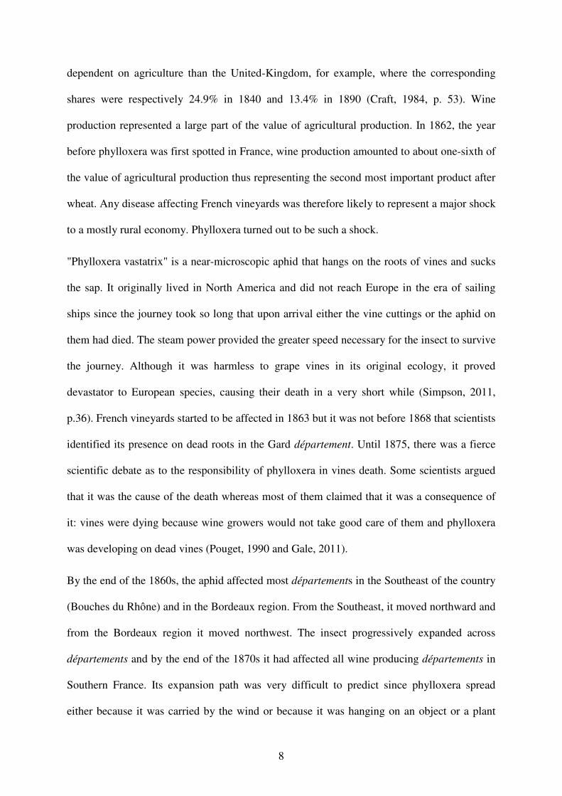
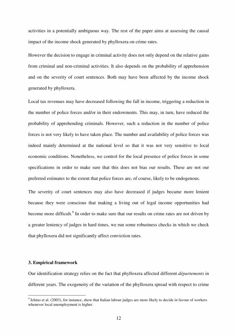
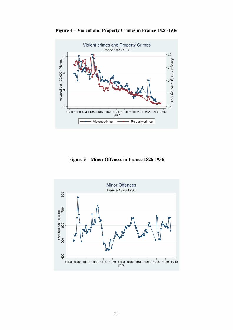
As illustrated on Figures 4 and 5, violent and property crimes decreased sharply over the

century whereas minor offences remained roughly constant. These general trends are taken

into account by including year fixed effects in our regressions.

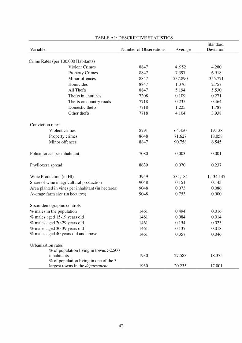
We also compute conviction rates for each type of crime and offence by dividing the number

of people convicted by the number of people accused in each département every year. The

corresponding rates vary from 64% for violent crimes to 72% for property crimes and 91% for

minor offences – see Appendix Table A1.

Finally, The Compte also provides information on police forces. More precisely, we know the

yearly number of urban and rural policemen, superintendents, forest wardens and guardsmen

10 Census data are available every five years only. In order to get yearly data for population at the département level, we interpolate Census data using growth rates of population between Census years - see Data appendix.

16

in each court-of-appeal jurisdiction between 1843 and 1932.11 We compute an indicator of the

presence of police forces defined as the ratio of the total number of police forces divided by

the population in each court-of-appeal jurisdiction. Over the period we study, there were on

average 3 members of police forces for 1,000 inhabitants in France (see Appendix Table A1).

4.2. Phylloxera

We build a département-year varying indicator of the presence of phylloxera. Since our

objective is to capture the timing of the shock to the local economy caused by the aphid, and

because the time span it took the insect to spread out and negatively affect wine crops

strongly varied across départements, it cannot be captured by a single lag structure. Galet,

(1957) provides information on the year when phylloxera was first spotted in at least one

municipality of each département and the year when the département was fully affected. We

exploit this information as follows. For each département we define year a as the year when

the aphid was first spotted and year b as the full-contagion year, that is the year when all

arrondissements – subdivisions of départements – were affected by phylloxera.

We then define the phylloxera indicator pij for département i at year j as a variable taking

values:

The phylloxera indicator thus takes value 1/(b-a+1) the first year the aphid is spotted in the

département. It then grows at rate 1/(b-a+1) until year b when the whole département is

affected. pij then takes value 1 until 1890, when the solution to the disease was implemented

on the entire French territory. Let's take the example of the Gard département. Phylloxera was

first spotted there in 1863 and the whole département was completely affected in 1878. In this

11 The data are actually available at the court (i.e. infra-département) level for 1843-1862, at the département level for 1879-1885 and at the court-of-appeal level for 1863-1878 and 1886-1932. We aggregate them at the court-of-appeal level for all years between 1843 and 1932. There were 27 courts of appeal in France in 1826.

17

case pij takes value 0.0625 in 1863, 0.125 in 1864 etc. until 1878 when it takes value 1 up to

1890. This definition of pij takes into account that the aphid spread out at a different pace in

the various départements thus taking a variable amount of time to fully affect wine production

and hence income.12

As shown by Figure 2, phylloxera had been spotted in 3.3% of the 87 French départements in

1865 whereas this figure amounted to 50.5% in 1880 and 71.3% in 1890. The first

département to be totally affected by phylloxera was Vaucluse in 1875. This was the case of

17% of all départements in 1880.

4.3. Wine production, wine intensity and farm size

Data on wine production are drawn from Galet (1957). In our dataset, the number of

hectolitres of wine produced is available for all départements between 1850 and 1905. Wine

was produced in 79 out of the 87 French départements in 1862 – i.e. the year before

phylloxera was first spotted in France.

Using information provided by the 1862 Agriculture Survey, we compute a couple of

measures of wine intensity in the various départements before phylloxera was first spotted in

France. We first compute the share of wine in agricultural production as of 1862: it is larger

than 15% in 39 départements. We also use data on the surface planted in vines per inhabitant

in 1862: the French average is as high as 0.07 ha (see Appendix Table A1). Eventually, we

compute the average farm size in each département in 1862: it is equal to 0.75 ha. We use

these variables in specifications in which we allow the impact of phylloxera on crime rates to

12 Banerjee et al. (2010) use an alternative strategy to overcome the lack of common lag structure capturing the time span taken by the insect to spread out. They define a phylloxera indicator which takes value 1 when phylloxera has been spotted in the département and wine production is at least 20% lower than in the last pre-phylloxera year. Despite all our results are robust to this specification (available upon request) this does not appear as an appropriate solution in our case since wine production might be directly affected by crime rates thus introducing a reverse causality bias.

18

vary according to the importance of wine-related activities and/or farm size in each

département as of 1862.

4.4 Control variables

We include socio-demographic controls in some robustness checks. Using the data from the

Statistique Générale de la France available since 1851, we compute the ratio of males in the

département population. We also control for the age structure of the male population, i.e. the

ratio of males aged 15-19, 20-29, 30-39 and 40 years old and above. Since these data come

from the Census which is available every 5 years only, we regress a 5-year moving average of

crime rates on a 5-year moving average of our phylloxera indicator and the socio-

demographic variables.13

We use a similar specification when controlling for urbanization. The data come from the

INED-Urbanisation database and are also available for Census years only.14 We compute the

proportion of people living in towns with more than 2,500 inhabitants – which is the standard

definition of a town in France (see Pumain and Guérin-Pace, 1990) - and the proportion of

people living in the 3 largest cities in the département. We control alternatively for each of

these two measures of urbanisation in order to make sure that our results are not due to

changes in the urban structure of the French départements that would be correlated with the

presence of phylloxera. Descriptive statistics of these variables are provided in Appendix

Table A1.

13 The 5-year moving averages are computed around census years. 14 See Pumain and Riandey (1986) for a thorough description of the data.

19

5. Results

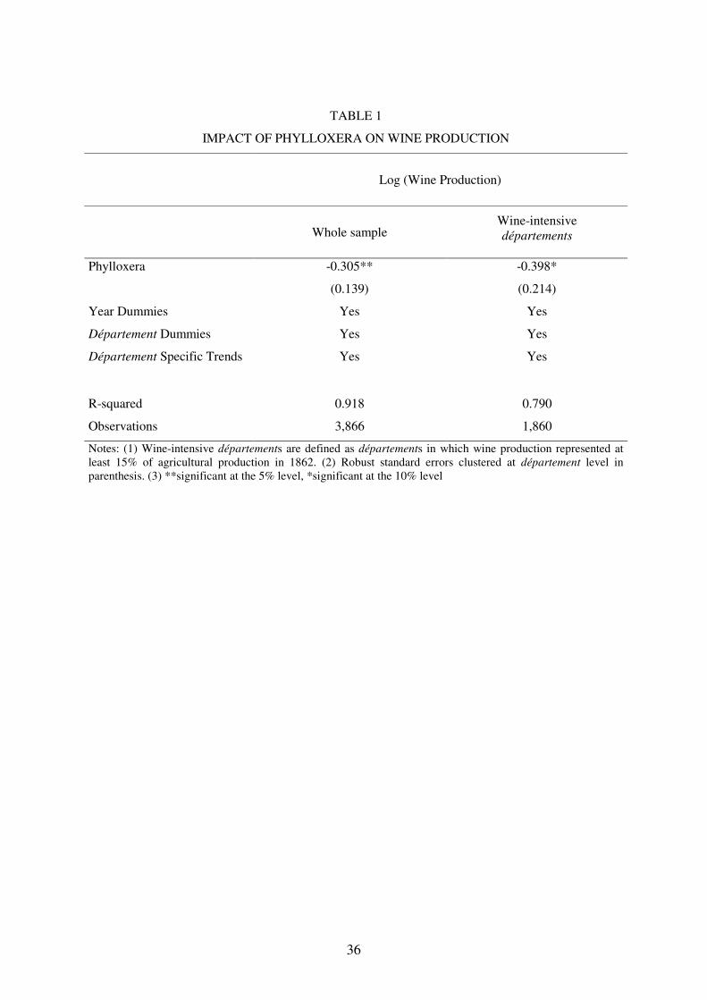
5.1 Phylloxera and wine production

Our empirical strategy relies on the fact that phylloxera generated a sharp drop in wine

production. We first check that this has actually been the case – see equation (1). Results are

reported in Table 1. During the phylloxera crisis, wine production is dramatically affected and

it falls by about 30% in an average year of full phylloxera contagion with respect to the period

of absence of phylloxera in the affected départements.15 In wine-intensive départements,

defined as those départements where wine production amounted to at least 15% of

agricultural production in 1862, the result is even stronger since we observe a drop of wine

production of about 40 per cent in the full-phylloxera period with respect to non-phylloxera

years.

These results show that the phylloxera pest provides an ideally strong exogenous shock on

wine production. It is worth noting here that with respect to using meteorological variables,

phylloxera not only has the advantage of not having an impact on deterrence costs but it

plausibly provides a stronger shock on wine production than variations in meteorological

variables (Chevet, Lecocq and Visser, 2011).

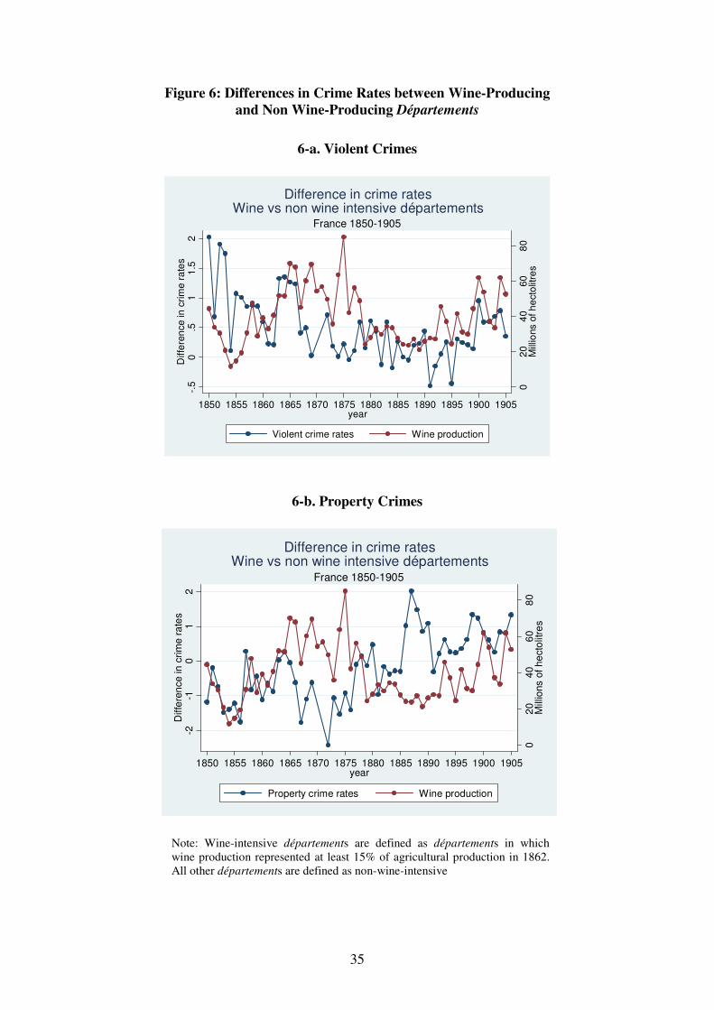
Figures 6a-b provide some preliminary evidence that the economic crisis brought about by the

fall in wine production following the diffusion of phylloxera caused an increase in some types

of crimes. We report trends in differences in crime rates between wine-intensive and non-

wine-intensive départements along with wine production. Figure 6a suggests that property

crimes rose more in wine-intensive than in non-wine-intensive départements when wine

production declined. This has been particularly true during the phylloxera period. In contrast,

the gap is not quite as striking for violent crimes. The rest of this section provides direct

estimates of the impact of phylloxera on crime rates.

15 These results are in line with Banerjee et al. (2010) who find a 35 per cent drop in wine production using a different indicator of phylloxera.

20

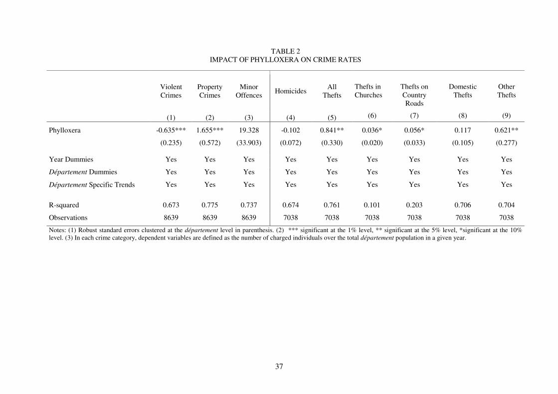
5.2. Phylloxera and crime: baseline results

In Table 2, we report the results obtained when estimating the model presented in equation

(2). All specifications include time and département dummies along with département-

specific time trends and standard errors are clustered at the département level. Columns (1) to

(3) report the results for aggregate crime categories. As evidenced in column (2) phylloxera

had a positive and significant impact on property crimes. Moving from the absence of

phylloxera to full contagion increased property crime rates by 1.655 per thousand points, i.e.

an average 22%. This suggests that the negative impact of phylloxera on legal earnings

opportunities dominated its potential damage to the quality of illegal activities. Despite we do

not have data on unemployment for 19th century France, these results are consistent with

papers showing that the quality and quantity of legitimate employment opportunities are pro-

cyclical and negatively related to crime rates (see Cook and Zarkin, 1985, and Mocan and

Bali, 2010).

Interestingly, the opposite effect is found for violent crimes – see column (1): full contagion

by phylloxera reduced violent crime rates by about 13%. This result is consistent with Traxler

and Burhop's (2010) who showed for 19th century Germany that when rainfalls used to be

particularly strong thereby generating an increase in rye prices – used to produce beer -,

violent crimes went down. However, this negative effect vanishes once accounted for beer

consumption. Together with our results, this suggests that, when hit by a negative income

shock, people reduce their consumption, including that of alcoholic drinks. As a consequence,

they engage less often in violent behaviour. As underlined by Melhum et al. (2006), "this is

the likely channel that reduces violent crime".16 In contrast, phylloxera does not seem to have

affected minor offences: the coefficient on the phylloxera variable is positive but insignificant

at conventional levels.

16 Melhum et al. (2006) p. 373.

21

Evidence regarding more disaggregated types of crimes is consistent with these initial

findings – columns (4) to (9). The impact of phylloxera on homicides was negative, although

not quite significant. In contrast, phylloxera increased the number of thefts per inhabitant –

see column (5). This was essentially driven by an increase in the number of thefts in churches,

thefts on country roads and a residual category including, among others, violent thefts.

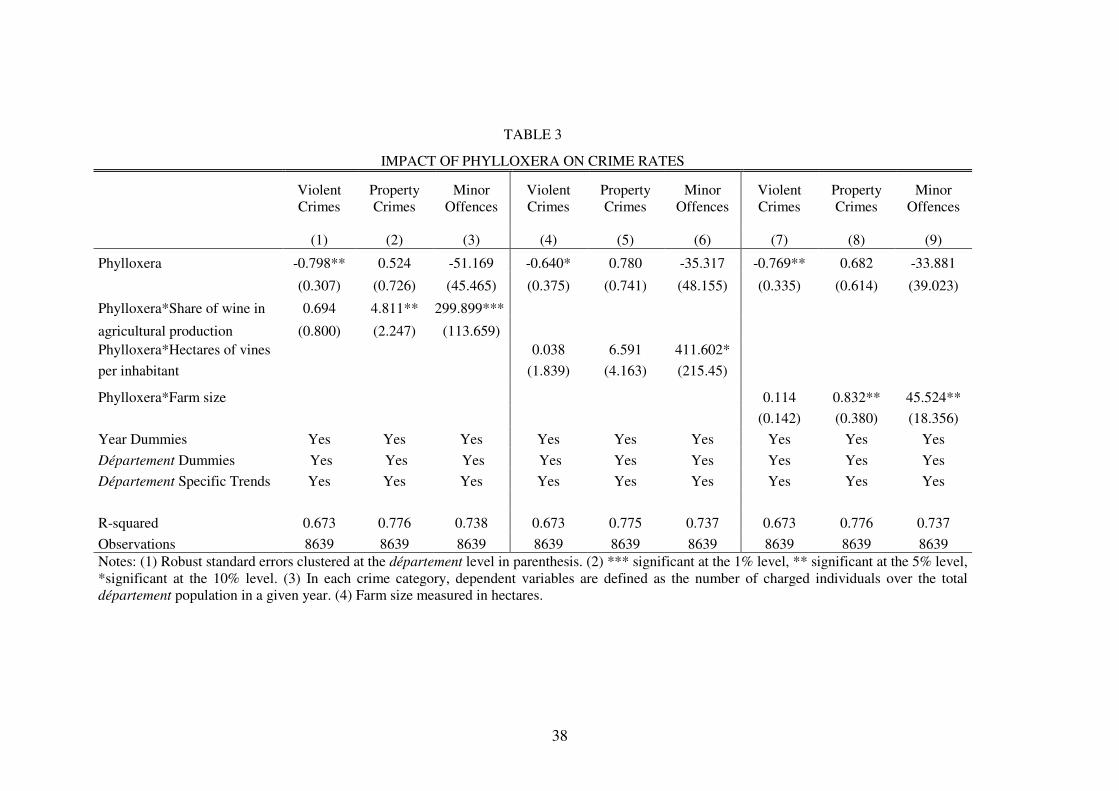
In order to better understand the role of local structures of agricultural production in our

findings, we run difference-in-difference estimates in which we compare the impact of

phylloxera in départements where wine growing represented a large proportion of economic

activity and in départements where this was not the case – and similarly for départements

with large vs. small farm size – see equation (3) and Table 3. More specifically, we interact

our phylloxera indicator with the share of wine in agricultural production in 1862 on the one

hand - columns (1) to (3) - and with the area planted in vine per inhabitant in 1862 on the

other hand - columns (4) to (6). This first set of results suggests that phylloxera had a larger

impact on property crimes in départements where wine initially represented a large share of

agricultural production. We also find a significant differential effect of phylloxera on minor

offences in wine-intensive départements: the interaction between phylloxera and the share of

wine in agricultural production is positive and significant at the 1% level, while the

interaction with the area planted in vines is significant at the 10% level. In contrast, the

negative effect of phylloxera on violent crimes does not seem to vary according to the

importance of wine in the local pre-phylloxera economy.

As a next step, we interact phylloxera with the average farm size in each département as of

1862. As shown in columns (8) and (9), the interaction term is positive and strongly

significant both for property crimes and minor offences. This suggests that the effect of

phylloxera was stronger in départements where farms were on average larger. One plausible

explanation for this finding is that wherever farms were large, wine growers employed many

22

workers. When phylloxera hit those départements and destroyed the vineyards, workers lost

their job, which left them without any income. In contrast, in regions with smaller farms,

salaried workers were fewer. Phylloxera strongly affected the small independent winegrowers

but it is likely that their means of support did not go down to an absolute zero since they

owned some land and could partially hedge against the income shock caused by phylloxera by

growing crops for self-consumption. So, the number of people ending up into absolute

poverty was presumably larger in large-farm areas. If increases in property crime and minor

offence rates were triggered by the lack of legal earnings opportunities, this may account for

their larger increase in large-farm départements.

Taken together, these results show that the negative income shock induced by the phylloxera

crisis strongly affected French crime rates. It caused a substantial increase in property crimes

while inducing a decrease in violent crimes probably due to the reduction in alcohol

consumption.17 These results suggest that, in the absence of a safety net provided by the

welfare state and given that the credit market itself was affected, engaging in property crime

turned out to be a way, for the French rural population, to cope with the negative economic

consequences of the phylloxera crisis.

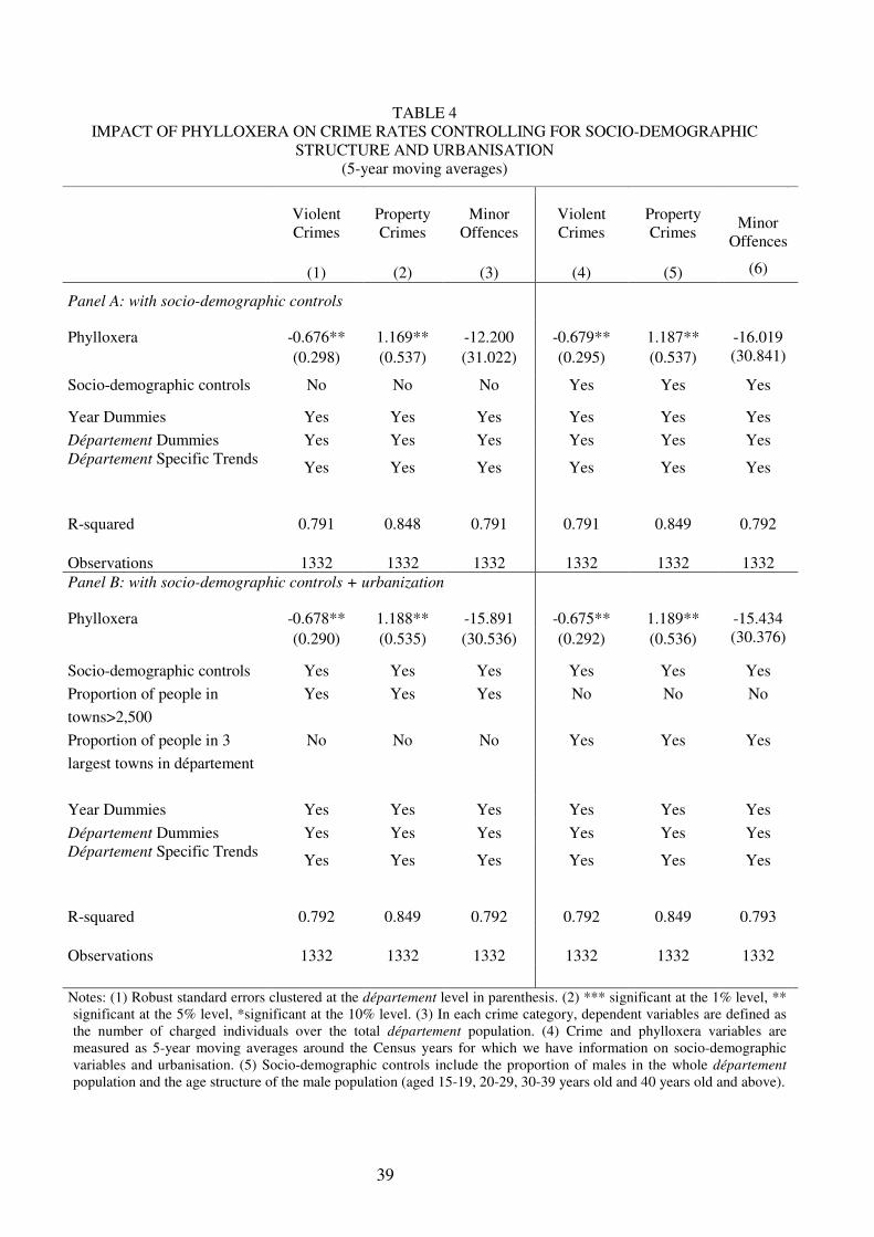
5.3. Robustness Checks

In the previous section, we provided evidence that the diffusion of phylloxera was associated

with an increase in property crime rates and a decrease in violent crimes. We have maintained

that the main channel driving our results is a negative shock on the income of people whose

main source of revenue was related to wine production.

In order to make sure that phylloxera does not capture the effect of other time-varying factors,

one may want to include a number of control variables. Socio-demographic controls are

17 This explanation is consistent with evidence reported in other studies showing a positive correlation between alcohol consumption and crime, e.g. Cook and Moore (1993) and Carpenter and Dobkin (2011).

23

natural candidates. Such variables are available for Census years only – see Data Section – so

that we re-estimate our baseline equation for 5-year moving averages computed around

Census years – see equation (4). As a first step, we check that this new specification does not

modify our results. As evidenced in Table 4 - Panel A - columns (1) to (3) – our results are

unchanged: moving from no-phylloxera to full contagion increases property crimes and

reduces violent crimes in a significant way. Introducing controls for the share of males in the

département population and for the age structure of the male population – see Panel A,

columns (4) to (6) – yields virtually identical results. This is not much of a surprise given that,

in order to bias our results, socio-demographic factors should have been correlated both with

crime rates and with the expansion of phylloxera, which was indeed quite unlikely.

Urbanisation may be a more serious concern if its intensity varied a lot across départements.

Panel B of Table 4 controls alternatively for the share of the département population living in

towns larger than 2,500 inhabitants – the standard definition of towns in France (see Section

4) – and the proportion living in the three largest cities in the département. Both specifications

leave our results unchanged: phylloxera still increases property crimes and reduces violent

crimes.

According to our interpretation, the positive effect of phylloxera on property crime rates is

due to the deterioration of the quality and quantity of labour opportunities which induced a

number of people to increase their amount of illegal activities with respect to legal ones. An

alternative mechanism consistent with our results would be related to the response of the

criminal justice system to crime. Reduced national and local tax collection during bad times

may result in reduced budgets for police forces and a subsequent reduction in the capacity of

the criminal justice system to contain crime. In order to control for this potential alternative

mechanism we include police forces measured at the court-of-appeal level in our regression.

Results are reported in Table 5. The coefficients on property and violent crimes are essentially

24

unaltered with respect to the baseline results. This suggests that police forces are unlikely to

have been endogenous, which is consistent with the fact that their allocation was mainly

determined at the national level. This test allows us ruling out that our results are driven by a

radical change in the presence of police forces at the local level as a consequence of the

phylloxera crisis.

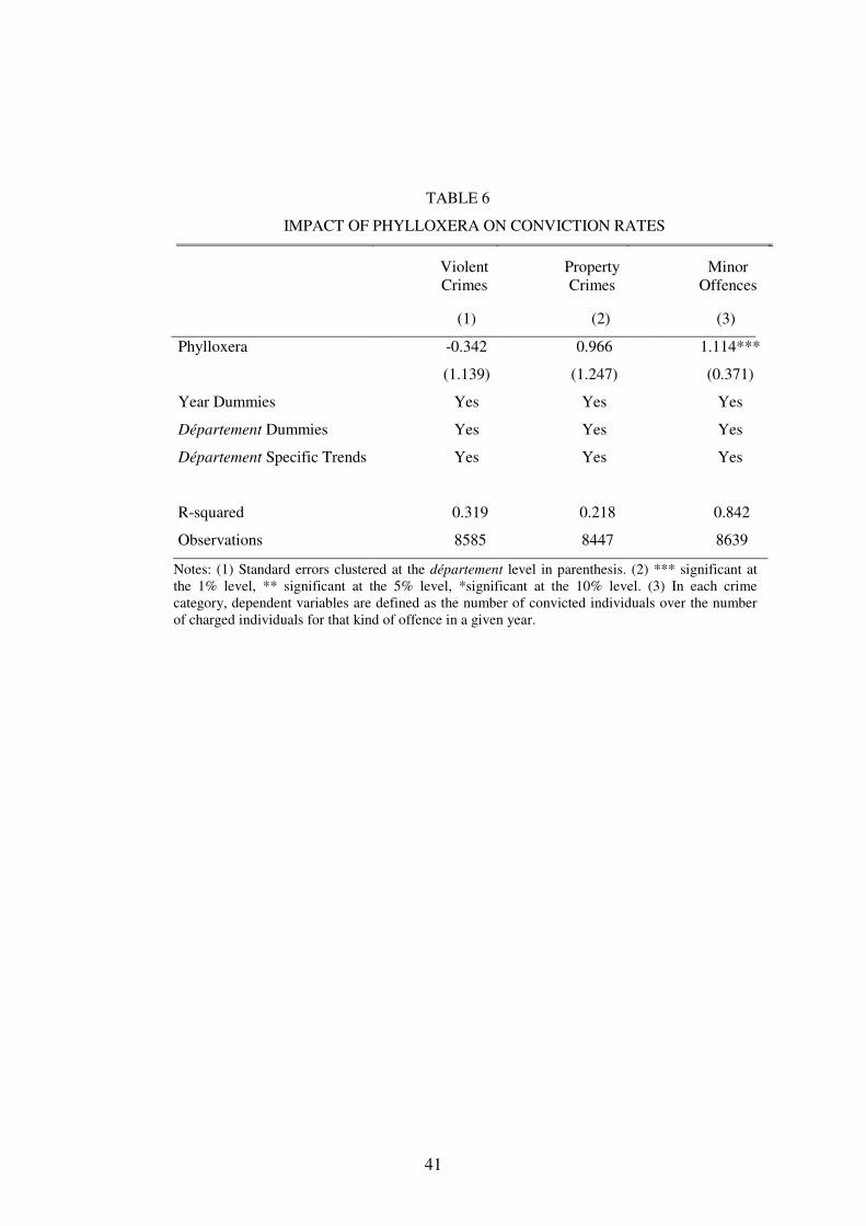
A second potential alternative mechanism through which the phylloxera crisis could have

affected crime rates is the behaviour of judges. During bad times, judges and juries could be

more lenient toward those committing property crimes as they might justify misbehaviour as a

consequence of the need to survive. If this were the case, the overall deterrence of the

criminal justice system would be reduced as a consequence of the phylloxera attack. Note that

in order for changes in leniency to account for our findings, judges should also have become

tougher to people committing violent crimes. In order to check for this alternative

explanation, we re-run our baseline equation for conviction rates as a dependent variable.

Results provided in Table 6 show that our phylloxera indicator does not significantly predict

conviction rates for violent and property crimes. As such, more lenient or tougher judges are

not likely to account for our main results.

As evidenced in column (3), things are quite different for minor offences: the coefficient on

the phylloxera indicator is positive and significant. The deterrence effect generated by this

change in judges' behaviour may account for the fact that, despite the negative income shock

brought about by phylloxera, we do not see any increase in minor offences. The difference we

find for conviction rates between minor offences and crimes may be explained by some

institutional characteristics of the French judicial system. Violent and property crimes were

judged by criminal courts in which juries were composed of randomly drawn registered voters

who decided both on guiltiness and mitigating circumstances while professional judges were

responsible for deciding sentences. In contrast, for minor offences, both jurors and court

25

presidents were professional judges - appointed by the Ministry of Justice - who may have

tried to counterbalance the potential effect of local economic conditions on minor offences.

6. Conclusions

This paper studies the effects of a large negative economic shock on crime using a unique

dataset based on 19th century French administrative crime records at the département level.

Our results show that the phylloxera crisis generated a 22% increase in property crime rates,

plausibly driven by the impact of phylloxera on the economic conditions of those living in the

affected départements. These results are robust to various alternative explanations including

possible changes in the criminal justice system or in the local presence of police forces

following the phylloxera crisis. Our findings are consistent with the standard economic model

of crime and suggest that property crimes, and in particular thefts, may have been used by

some of the French rural population in the 19th century as a risk coping strategy.

Moreover, we show that the diffusion of phylloxera brought about a substantial decrease in

violent crime rates (- 13%) consistent with the idea that the income shock induced a drop in

alcohol consumption. This finding is in line with results by Melhum et al. (2006) and Traxler

and Burhop (2010) who provide evidence of a reduction in violent crimes following the fall in

beer consumption brought about by bad rye crops in 19th century German states.

Despite it is very difficult to draw policy conclusions from an exercise not designed to test the

effect of a specific policy, our findings are consistent with the idea that an insurance

mechanism against negative income shocks may prevent the latter from generating a strong

increase in property crime rates. These conclusions are in line with the implications of other

studies focusing on developing countries today. In particular, Miguel (2005) concludes that in

order to reduce the number of old women homicides induced as a response to an increase in

poverty after extreme weather events in rural Tanzania it would be desirable to improve both

26

the insurance system against extreme rain falls and provide pensions to people in extreme

poverty. Of course, as also discussed by Miguel (2005), an alternative solution could be to

increase deterrence. Our results on minor offences suggest that this could be done by ensuring

that judges become tougher when economic conditions deteriorate. However this solution

may be difficult to implement if judges are truly independent. Moreover, an increase in the

severity of sentences could be particularly costly since it could trigger an increase in

incarceration rates.

27

References

Annuaire statistique de la France, 1946, Paris : Imprimerie Nationale.

Arambourou R. 1958. "Cadastre et Sociologie Electorale", Revue Française de Science

Politique, 8(2), 368-383.

Banerjee, A, E. Duflo, G. Postel-Vinay and T. Watts. 2010. "Long Run Health Impacts of

Income Shocks: Wine and Phylloxera in 19th Century France", Review of Economics and

Statistics, 92(4), 714-728.

Becker G. 1968. "Crime and Punishment: an economic approach", Journal of Political

Economy, 76(2), 169-217.

Buonanno, P. and D. Montolio. 2008 "Identifying the Socio-economic and Demographic

Determinants of Crime across Spanish Provinces". International Review of Law and

Economics, 28(2), 89-97.

Carbasse, J-M. 2000. Histoire du Droit Pénal et de la Justice Criminelle, Paris: Presses

Universitaires de France, 2nd edition.

Carpenter, C. and Dobkin, C. 2011 “Alcohol Regulation and Crime” in Cook, P. Ludwig, J.

and McCrary, J. (Eds.) Controlling Crime: Strategies and Tradeoffs, Chicago: University of

Chicago Press, 291-329.

Chevet, J.-M., S. Lecocq and M. Visser. 2011. "Climate, grapevine phenology, wine

production and prices: Pauillac (1800-2009)". American Economic Review Papers and

Proceedings, 101(3), 142-146.

Cook, P.J and G. Zarkin. 1985. "Crime and the business cycle.", Journal of Legal Studies, 14,

115-128.

28

Cook, P.J. and M.J. Moore. 1993. "Economic perspectives on alcohol-related violence", in:

S.E. Martin, ed., Alcohol-Related Violence: Interdisciplinary Perspectives and Research

Directions. NIH Publication No. 93-3496.

Craft, N.F.R. 1984. "Economic Growth in France and Britain, 1830-1910: A Review of the

Evidence", Journal of Economic History 44(1), 49-67.

Fajnzylber, P., D. Lederman and N. Loayza. 2002. "What Causes Violent Crimes?",

European Economic Review, 46(7), 1323-57.

Fafchamps, M. and B. Minten. 2006. "Crime, Transitory Poverty, and Isolation: Evidence

from Madagascar". Economic Development and Cultural Change, 54(3), 579-603.

Fougère, D., F. Kramarz and J. Pouget. 2009. "Youth Unemployment and Crime in France."

Journal of the European Economic Association, 7(5), 909-938.

Gale George. 2011. Dying on the Vine. How Phylloxera Transformed Wine, Berkeley:

University of California Press.

Galet, P. 1957. Cépages et vignobles de France, Montpellier, Imprimerie du Paysan du Midi.

Gould, E., B. Weinberg, and D. Mustard. 2002. "Crime Rates and Local Labor Market

Opportunities in the United States: 1979-1997", The Review of Economics and Statistics,

84(1), 45-61.

Ichino, A., M. Polo and E. Rettore. 2003. "Are Judges Biased by Labor Market Conditions?",

European Economic Review, 47 (5), 913-944 .

Lagrange, H. 2003. "Crime and Socio-Economic Context.", Revue Française de Sociologie,

44, 29-48.

Lin, M. 2008. "Does Unemployment Increase Crime?: Evidence from U.S. Data 1974–2000",

Journal of Human Resources, 43(2), 413-436.

29

Loubère Leo A. 1978. The Red and the White. A History of Wine in France and Italy in the

19th Century, New-York: State University of New-York Press.

Machin, S. and C. Meghir. 2004. "Crime and Economic Incentives," Journal of Human

Resources, 39(4), 958-979.

Maddison, A. 1995. Monitoring the World Economy, 1820-1992, Paris, OECD Development

Center Studies.

Melhum, H., E. Miguel and R. Torvik. 2006. "Poverty and Crime in 19th Century Germany",

Journal of Urban Economics, 59(3), 370-388.

Miguel, E. 2005. "Poverty and Witch Killing", Review of Economic Studies, 72(4), 1153-

1172.

Mocan, N . and T. Bali. 2010. "Asymmetric Crime Cycles", Review of Economics and

Statistics, 92(4), 899-911.

Occhino F., K. Oosterlinck and E. White. 2008. "How Much can a Victor force the

Vanquished to Pay?", Journal of Economic History, 68(1), 1-45.

Oster, A., and J. Agell. 2007. "Crime and unemployment in turbulent times." Journal of the

European Economic Association, 5(4), 752-775.

Ordish George. 1972. The Great Wine Blight, London: J.M. Dent and Sons Ltd.

Perrot, M. and P. Robert. 1989. Compte Général de l'Administration de la Justice Criminelle

en France pendant l'année 1880 et Rapport relatif aux années 1826 à 1880, Genève: Slatkine

Reprints.

Postel-Vinay, G. 1989. “Debts and Agricultural Performance in the Languedocian Vineyard,

1870–1914”., in G. Grantham and C. S. Leonard (Eds.), Agrarian Organization in the

30

Century of Industrialization: Europe, Russia, and North America; Greenwich, CT: JAI Press,

161–186.

Pouget, R. 1990. Histoire de la lutte contre le phylloxéra de la vigne en France : 1868-1895,

Paris, Institut national de la recherche agronomique.

Pumain D. and F. Guérin-Pace. 1990. "150 ans de Croissance Urbaine", Economie et

Statistiques, 230(1), 5-16.

Pumain D. and B. Riandey. 1986. "Le Fichier de l'INED: Urbanisation de la France", Espace,

Populations, Sociétés, 1986(2), 269-277.

Toutain, J.-C. 1987. Le produit intérieur brut de la France de 1789 à 1982, Paris: Économies

et sociétés : Histoire quantitative de l'économie française.

Traxler, C. and C. Burhop. 2010. "Poverty and crime in 19th century Germany: A

reassessment.", Max Planck Institute for Research on Collective Goods, Working Paper 2010-

35.

31

Figure 1 – Violent crimes, property crimes and GDP per capita

1-a Violent Crimes

100

01

50

02

00

02

50

03

00

03

50

01

99

0 U

S D

olla

rs

34

56

78

Accu

sed

per

10

0,0

00

1820 1830 1840 1850 1860 1870 1880 1890 1900 1910 1920year

Violent crimes GDP per capita

France 1826-1913

Violent crimes and GDP per capita

Source: authors' computations from Compte Général de la Justice Criminelle, Annuaire Statistique de la France and Maddison (1995).

1-b Property Crimes 1

00

01

50

02

00

02

50

03

00

03

50

01

99

0 U

S D

olla

rs

05

10

15

20

Accu

sed

per

10

0,0

00

1820 1830 1840 1850 1860 1870 1880 1890 1900 1910 1920year

Property crimes GDP per capita

France 1826-1913

Property crimes and GDP per capita

Source: authors' computations from Compte Général de la Justice Criminelle, Annuaire Statistique de la France and Maddison (1995).

32

Figure 2. Phylloxera and Share of Wine Production in GDP, 1862-1890

0

20

40

60

80

as %

of d

épa

rte

me

nts

2

4

6

8

as %

of G

DP

1860 1870 1880 1890year

Share of wine production

Share of départements affected by phylloxera

France 1862-1890

Phylloxera and Share of Wine Production in GDP

Source: authors' computations from Annuaire Statistique de la France (1946), Toutain (1987) and Galet (1957) Statistique de la France and Maddison (1995).

33

Figure 3 - Compte Général de la Justice Criminelle, 1869

34

Figure 4 – Violent and Property Crimes in France 1826-1936

05

10

15

20

Accuse

d p

er

100

,00

0 -

Pro

pe

rty

24

68

Accu

se

d p

er

100

,00

0 -

Vio

len

t

1820 1830 1840 1850 1860 1870 1880 1890 1900 1910 1920 1930 1940year

Violent crimes Property crimes

France 1826-1936

Violent crimes and Property Crimes

Figure 5 – Minor Offences in France 1826-1936

40

050

060

070

080

0A

ccuse

d p

er

10

0,0

00

1820 1830 1840 1850 1860 1870 1880 1890 1900 1910 1920 1930 1940year

France 1826-1936

Minor Offences

35

Figure 6: Differences in Crime Rates between Wine-Producing

and Non Wine-Producing Départements

6-a. Violent Crimes

02

04

06

08

0M

illio

ns o

f h

ecto

litre

s

-.5

0.5

11

.52

Diffe

ren

ce in

crim

e r

ate

s

1850 1855 1860 1865 1870 1875 1880 1885 1890 1895 1900 1905year

Violent crime rates Wine production

France 1850-1905

Difference in crime ratesWine vs non wine intensive départements

6-b. Property Crimes

02

04

06

08

0M

illio

ns o

f h

ecto

litre

s

-2-1

01

2D

iffe

ren

ce in

crim

e r

ate

s

1850 1855 1860 1865 1870 1875 1880 1885 1890 1895 1900 1905year

Property crime rates Wine production

France 1850-1905

Difference in crime ratesWine vs non wine intensive départements

Note: Wine-intensive départements are defined as départements in which wine production represented at least 15% of agricultural production in 1862. All other départements are defined as non-wine-intensive

36

TABLE 1

IMPACT OF PHYLLOXERA ON WINE PRODUCTION

Log (Wine Production)

Whole sample

Wine-intensive départements

Phylloxera -0.305** -0.398*

(0.139) (0.214)

Year Dummies Yes Yes

Département Dummies Yes Yes

Département Specific Trends Yes Yes

R-squared 0.918 0.790

Observations 3,866 1,860

Notes: (1) Wine-intensive départements are defined as départements in which wine production represented at least 15% of agricultural production in 1862. (2) Robust standard errors clustered at département level in parenthesis. (3) **significant at the 5% level, *significant at the 10% level

37

TABLE 2 IMPACT OF PHYLLOXERA ON CRIME RATES

Violent Crimes

Property Crimes

Minor Offences Homicides All

Thefts Thefts in Churches

Thefts on Country Roads

Domestic Thefts

Other Thefts

(1) (2) (3) (4) (5) (6) (7) (8) (9)

Phylloxera -0.635*** 1.655*** 19.328 -0.102 0.841** 0.036* 0.056* 0.117 0.621**

(0.235) (0.572) (33.903) (0.072) (0.330) (0.020) (0.033) (0.105) (0.277)

Year Dummies Yes Yes Yes Yes Yes Yes Yes Yes Yes

Département Dummies Yes Yes Yes Yes Yes Yes Yes Yes Yes

Département Specific Trends Yes Yes Yes Yes Yes Yes Yes Yes Yes

R-squared 0.673 0.775 0.737 0.674 0.761 0.101 0.203 0.706 0.704

Observations 8639 8639 8639 7038 7038 7038 7038 7038 7038

Notes: (1) Robust standard errors clustered at the département level in parenthesis. (2) *** significant at the 1% level, ** significant at the 5% level, *significant at the 10% level. (3) In each crime category, dependent variables are defined as the number of charged individuals over the total département population in a given year.

38

TABLE 3

IMPACT OF PHYLLOXERA ON CRIME RATES

Violent Crimes

Property Crimes

Minor Offences

Violent Crimes

Property Crimes

Minor Offences

Violent Crimes

Property Crimes

Minor Offences

(1) (2) (3) (4) (5) (6) (7) (8) (9)

Phylloxera -0.798** 0.524 -51.169 -0.640* 0.780 -35.317 -0.769** 0.682 -33.881

(0.307) (0.726) (45.465) (0.375) (0.741) (48.155) (0.335) (0.614) (39.023)

Phylloxera*Share of wine in 0.694 4.811** 299.899***

agricultural production (0.800) (2.247) (113.659) Phylloxera*Hectares of vines 0.038 6.591 411.602* per inhabitant (1.839) (4.163) (215.45)

Phylloxera*Farm size 0.114 0.832** 45.524** (0.142) (0.380) (18.356) Year Dummies Yes Yes Yes Yes Yes Yes Yes Yes Yes Département Dummies Yes Yes Yes Yes Yes Yes Yes Yes Yes Département Specific Trends Yes Yes Yes Yes Yes Yes Yes Yes Yes R-squared 0.673 0.776 0.738 0.673 0.775 0.737 0.673 0.776 0.737 Observations 8639 8639 8639 8639 8639 8639 8639 8639 8639 Notes: (1) Robust standard errors clustered at the département level in parenthesis. (2) *** significant at the 1% level, ** significant at the 5% level, *significant at the 10% level. (3) In each crime category, dependent variables are defined as the number of charged individuals over the total département population in a given year. (4) Farm size measured in hectares.

39

TABLE 4 IMPACT OF PHYLLOXERA ON CRIME RATES CONTROLLING FOR SOCIO-DEMOGRAPHIC

STRUCTURE AND URBANISATION (5-year moving averages)

Violent Crimes

Property Crimes

Minor Offences

Violent Crimes

Property Crimes Minor

Offences

(1) (2) (3) (4) (5) (6)

Panel A: with socio-demographic controls

Phylloxera -0.676** 1.169** -12.200 -0.679** 1.187** -16.019 (0.298) (0.537) (31.022) (0.295) (0.537) (30.841)

Socio-demographic controls No No No Yes Yes Yes

Year Dummies Yes Yes Yes Yes Yes Yes Département Dummies Yes Yes Yes Yes Yes Yes Département Specific Trends Yes Yes Yes Yes Yes Yes

R-squared 0.791 0.848 0.791 0.791 0.849

0.792

Observations 1332 1332 1332 1332 1332

1332 Panel B: with socio-demographic controls + urbanization

Phylloxera -0.678** 1.188** -15.891 -0.675** 1.189** -15.434 (0.290) (0.535) (30.536) (0.292) (0.536) (30.376)

Socio-demographic controls Yes Yes Yes Yes Yes Yes Proportion of people in Yes Yes Yes No No No towns>2,500

Proportion of people in 3 No No No Yes Yes Yes largest towns in département

Year Dummies Yes Yes Yes Yes Yes Yes Département Dummies Yes Yes Yes Yes Yes Yes Département Specific Trends Yes Yes Yes Yes Yes Yes

R-squared 0.792 0.849 0.792 0.792 0.849

0.793

Observations 1332 1332 1332 1332 1332

1332 Notes: (1) Robust standard errors clustered at the département level in parenthesis. (2) *** significant at the 1% level, ** significant at the 5% level, *significant at the 10% level. (3) In each crime category, dependent variables are defined as the number of charged individuals over the total département population. (4) Crime and phylloxera variables are measured as 5-year moving averages around the Census years for which we have information on socio-demographic variables and urbanisation. (5) Socio-demographic controls include the proportion of males in the whole département

population and the age structure of the male population (aged 15-19, 20-29, 30-39 years old and 40 years old and above).

40

TABLE 5

IMPACT OF PHYLLOXERA ON CRIME RATES CONTROLLING FOR

POLICE FORCES

Violent Crimes

Property Crimes

Minor Offences

(1) (2) (3)

Phylloxera -0.473** 1.218** -4.322

(0.235) (0.499) (28.055)

Police Forces Yes Yes Yes

Year Dummies Yes Yes Yes

Département Dummies Yes Yes Yes

Département Specific Trends Yes Yes Yes

R-squared 0.663 0.723 0.767

Observations 6896 6896 6896

Notes: (1) Standard errors clustered at the département level in parenthesis. (2) *** significant at the 1% level, ** significant at the 5% level, *significant at the 10% level.(3) In each crime category, dependent variables are defined as the number of charged individuals over the total département population in a given year. (4) Police forces are defined as the ratio of the total number of police forces to the population in each court-of-appeal jurisdiction.

41

TABLE 6

IMPACT OF PHYLLOXERA ON CONVICTION RATES

Violent Crimes

Property Crimes

Minor Offences

(1) (2) (3)

Phylloxera -0.342 0.966 1.114***

(1.139) (1.247) (0.371)

Year Dummies Yes Yes Yes

Département Dummies Yes Yes Yes

Département Specific Trends Yes Yes Yes

R-squared 0.319 0.218 0.842

Observations 8585 8447 8639

Notes: (1) Standard errors clustered at the département level in parenthesis. (2) *** significant at the 1% level, ** significant at the 5% level, *significant at the 10% level. (3) In each crime category, dependent variables are defined as the number of convicted individuals over the number of charged individuals for that kind of offence in a given year.

42

TABLE A1: DESCRIPTIVE STATISTICS

Variable Number of Observations Average Standard Deviation

Crime Rates (per 100,000 Habitants) Violent Crimes 8847 4 .952 4.280 Property Crimes 8847 7.397 6.918 Minor offences 8847 537.890 355.771 Homicides 8847 1.376 2.757 All Thefts 8847 5.194 5.530 Thefts in churches 7208 0.109 0.271 Thefts on country roads 7718 0.235 0.464 Domestic thefts 7718 1.225 1.787 Other thefts 7718 4.104 3.938

Conviction rates

Violent crimes 8791 64.450 19.138 Property crimes 8648 71.627 18.058 Minor offences 8847 90.758 6.545

Police forces per inhabitant 7080 0.003 0.001 Phylloxera spread 8639 0.070 0.237 Wine Production (in Hl) 3959 534,184 1,134,147 Share of wine in agricultural production 9048 0.151 0.143 Area planted in vines per inhabitant (in hectares) 9048 0.073 0.086 Average farm size (in hectares) 9048 0.753 0.900 Socio-demographic controls % males in the population 1461 0.494 0.016 % males aged 15-19 years old 1461 0.084 0.014 % males aged 20-29 years old 1461 0.154 0.023 % males aged 30-39 years old 1461 0.137 0.018 % males aged 40 years old and above 1461 0.357 0.046 Urbanisation rates

% of population living in towns >2,500 inhabitants 1930 27.583 18.375 % of population living in one of the 3 largest towns in the département. 1930 20.235 17.001

43

Data Appendix

1. French départements

In 1826 there were 86 départements the borders of which were defined during the French

revolution. The main changes which took place between 1826 and 1936 were the following.

In 1860 three new départements were created with pieces of land coming from the duchy of

Savoy and the Nice county: Savoie, Haute-Savoie and Alpes Maritimes. They are included in

our database from 1861 onward.

In 1871 France lost the war against Prussia. The two Alsatian départements (Haut-Rhin and

Bas-Rhin) became German as well as part of both the Meurthe and the Moselle. The parts of

Meurthe and Moselle which remained French were merged into a new département called

Meurthe-et-Moselle. As a result of World War I, the territory which had become German in

1871 went back to France. A new département was created with the German part of Meurthe

and Moselle and was called Moselle. Haut-Rhin and Bas-Rhin are included in our database

from 1826 to 1869 and from 1919 to 1936. Given the impossibility to compare Meurthe,

Meurthe-et-Moselle and Moselle over time we drop them from our data.

The Belfort area was part of the Haut-Rhin département before 1871. Administratively, it

became part of Haute-Saône from 1871 to 1922. It then became an independent département

in 1922 under the name of Territoire de Belfort. Given this historical instability, we drop it

from our data.

2. Population

The population of each département comes from the Census which is available for years

1831, 1836, 1841, 1846, 1851, 1856, 1861, 1866, 1872, 1876, 1881, 1886, 1891, 1896, 1901,

1906, 1911, 1912, 1921, 1926, 1931 and 1936.

We compute yearly population by linearly interpolating observed population using the

population growth rate between two consecutive Census years. Years with wars fought on the

French territory are dropped (1870-1871 and 1914-1918). For years between Census and

wars, we proceed in the following way. For years 1867 to 1869 and for 1913, we extrapolate

the last Census population using the growth rate of the previous inter-Census period. For

years 1872 to 1875 and 1920-21, we retropolate the next Census population using the growth

44

rate of the following inter-Census period. The 1830 and 1848 revolutions had no noticeable

impact on département populations.

3. Crime data

Crime data come from the Compte Général de la Justice Criminelle. They are available for all

years between 1826 and 1936 except for the period from 1914 to 1918. For Haut-Rhin and

Bas-Rhin, crime data become available again after WWI in 1925.