Swedish Environmental Protection Agency

Impact of Fuels onExhaust Emissions

A chemical and biologicalcharacterization

Edited by

Roger WesterholmKarl-Erik Egebäck

I f THIS OOCUMLNT II I M U N B f l»IB

SW— 3968

EE92 563058

Impact of Fuels onDiesel Exhaust Emissions

A chemical and biologicalcharacterization

Edited by

Roger WesterholmStockholm UniversityStockholm, Sweden

Karl-Erik EgebäckSwedish Motor VehicleInspection CompanyStockholm, Sweden

MASTER•CTRI3UII0N IF THIS DOCUMENT B U U M T S

FN06N SMS PWWITB

The following report is based on work conductedwith economic support from the Research Commit-tee of Swedish Environmental Protection Agency,Saab-Scania, Volvo, SPI, The Association of Swed-ish Automobile Manufacturers and Whole Salers(BID, The County Council of Stockholm, NUTEKand TFB-

The authors assume sole responsibility for the con-tents of the report, which therefore, cannot becited as representing the viewpoint of the Envi-ronmental Protection Agency.

Solna in September, 1991Swedish Environmenal Protection AgencyResearch Department

The report has been submitted toexternal referees for checking.

ISSN 0282-7298ISBN 91-620-3968-7

Ordering address:NaturvårdsverketInformation DepartmentS-171 85 SOLNASWEDEN

Contents

Preface 5

Abstract 6

1 Background 7

2 Literature Survey 92.1 Summary of the Literature Survey 262.2 References 27

3 Experimental 303.1 Fuels 303.2 Vehicles 323.3 Test Programs 33

4 Regulated Exhaust Emiss ions 374.1 CARBON MONOXIDE 384.1.1 Results and Discussions 384.1.2 Conclusions 39

4.2 NITROGEN OXIDES 394.2.1 Results and Discussions 394.2.2 Conclusions 39

43 HYDROCARBONS 404.3.1 Results and Discussions 404.3.2 Conclusions 40

4 4 PARTICULATE EMISSIONS 404.4.1 Results and Discussions 404.4.2 Conclusions 41

Unregulated Exhaust Emiss ions 53ALDEHYDES 53

. 1 Introduction 53

.2 Materials and Methods 53

.3 Results and Discussions 54

.4 Conclusions 55

.5 References 55

5.2 PARTICULATE ANALYSIS AND SMOKE TEST 585.2.1 Introduction 585.2.2 Materials and Methods 585.2.3 Results and Discussions 595.2.4 References 61

5.35.3.15.3.25.3.35.3.45.3.55.45.4.15.4.25.4.35.4.45.4.55.55.5.15.5.25.5.35.5.45.5.55.6

5.6 15.6.25.6.3

66.16.1.16.1.26.1.36.1.46.1.56.26.2.16.2.26.2.36.2.46.2.5

7

OLEFINESIntroductionMaterials and MethodsResults and DiscussionsConclusionsReferencesOXYGENATES AND LIGHT AROMATICS COMPOUNDSIntroductionMaterials and MethodsResults and DiscussionsConclusionsReferencesPOLYCYCLIC AROMATIC COMPOUNDSIntroductionMaterials and MethodsResults and DiscussionsConclusionsReferencesCARBON DIOXIDES EMISSIONS AND FUELCONSUMPTIONIntroductionResults and DiscussionsConclusions

Biological TestingMUTAGENICITY TESTSIntroductionMaterials and MethodsResults and DiscussionsConclusionsReferencesDIOXIN RECEPTOR AFFINITY TESTSIntroductionMaterials and MethodsResults and DiscussionsConclusionsReferences

Conclusions

AppendixA:lA.2

A:2.1A:2.2A:2.3A:2.4A:2.f)

FUEL CHARACTERISTICSMULTIVARIATE ANALYSIS OF DIESEL FUELEMISSION DATAIntroductionStatisticsResults and DiscussionsConclusionsReferences

676767686969

727272737474808080848787

94949494

100100100iOi101104105115115116118121121

126

131

133133135137142142

Preface

In Europe nearly one hundred per cent of the engines for heavy dutyvehicles are diesel engines. The diesel engine has proven to be fuel efficientand reliable and. therefore, up until recent year judged to be the onlyalternative for heavy trucks and buses. The principal, and serious draw-backs of the diesel engine are the emissions. In Europe the estimation isthat road transport is responsible for the majority of anthropogenic emis-sions and "from 1985 - 1992 it is expected that road transport will increasefrom 50 'i to 70 '"> of the means of transport used to transport goods". < MikeWalsh: Car Lines, November 1990.) Comparing diesel exhaust emissionswith gasoline exhaust emissions, the main differences are the omissions ofCO and particles. For diesel engines the CO emission is not of greatconcern but the particulate emissions are considered to be one of the mainproblems. Diesel particles are suspected of causing special health problemsbecause they are very small and, therefore, likely to be deposited deep inthe lungs. In many studies it has been well shown that diesel particles aremutagenic and carriers of compounds which are suspected of contributingto the rise in cancer cases in city areas with a large proportion of dieselfueled vehicles.

Many efforts have been made to reduce the emission of pollutants fromdiestl fueled vehicles. The combustion process in the diesel engine does notallow the utilization of such measures as the three-way catalyst technique.Therefore, the engine manufacturers have to rely on other measures suchas improvement of the engine, oxidation catalysts or particular traps. Onemeasure of great importance, which must be acted up on. is the improve-ment of diesel fu««l. There are at least two advantages in using "cleaner"diesel fuels: firstly the direct beneficial effect on the emission and secondlythe indirect effect on the emission of particles, for example, when a catalystis used in the oxhaust system, sulfur in the fuel can he converted tosulfates during the catalytic process. It is as yet unsure whether sulfur andother contaminants in the fuel may lead to an accelerated deterioration ofcatalysts and particulate traps.

A joint project group was formed between The Swedish Motor VehicleInspection Company. Stockholm University and The Karolinska Institute,Stockholm, in order to study the effect on the exhaust emission when usingdifferent blends of diesel fuels in a bus and a truck. The investigation wasfinanced by an agreement between The Swedish Environmental ProtectionAgency and the Swedish Motor Vehicle Inspection Company and supportedby the project Air pollution in Urban Areas administrated by the SwedishEnvironmental Protection Agency. The results of the investigation arepresented in this report.

Abstract

Eight different diesel fuels were selected for the investigation. As theinvestigation primarily was aimed at finding a "good" diesei fuel to be usedfor vehicles operating in city areas, seven of the fuels were meant to besuch fuels. Six of the eight fuels had low sulfur content and one was areally low aromatic fuel. 1.8 %. The total aromatic content of the rest of the"good" fuels varied between 16.6 •?• to 25.1 f which is somewhat too high tobe a really "good" fuel. One common commercial fuel was used as areference for commercial fuels on the Swedish market. Of the seven otherfuels only three are commercially available and commonly used for citybuses. Two of these fuels are light diesel fuels (jet fuels) and one a blend ofdifferent kerosenes which has newly been introduced on the Swedishmarket.

Two vehicles, a bus and a truck, were used for this investigation. Thevehicles were checked and serviced by the manufacturers of the vehicles.All the tests were carried out by running the vehicles on a chassis dyna-mometer as per one steady state driving cycle and two different transientdriving cycles. The steady state cycle was the ECE 13 mode cycle, whichwas originally developed to be used for engine tests. The two transientdriving cycles were: Fahrcyklus fur Stadtlinien Omnibus.se termed the Buscycle and the U.S. Environmental Protection Agency (EPA» Driving Sched-ule for Heavy Duty Vehicles. Samples for analysis of the regulated emis-sions i.e. hydrocarbons (HO, carbon monoxide (CO) and nitrogen oxidesi NO,» were taken at all tests and samples of particle» at both of thetransient tests. In addition to the measurement of the regulated emissions,samples were taken for analysis of; aldehydes, oxygenates, light aromaticsand polycyclic aromatic compounds (PAC), and also for biological testing(mutagenicity tests and TCDD receptor affinity tests). Samples for analy-sis of the unregulated pollutions and for the biological testing were takenwhen running the vehicles according to the bus cycle. The samples weredrawn from a dilution tunnel when running the vehicles according to thetransient cycles.

The entire data material (regulated emissions, unregulated emissions,biological investigation data) are listed in an appendix which will bepublished as a separately publication "Appendix to Impact of Fuels onDiesel Exhaust Emissions". The appendix will be published in the .SwedishEnvironmental Protection Agency (SNV) report series.

According to the results of this investigation the most important furlparameters are density, 90 r/r distillation point, final boiling point, specificheat, aromatics, sulfur and PAC content.

In summing up the results of this study it can be observed that there existsa quantifiable relationship between the variables of the diesel fuel blendsand the variables of the chemical emission and their biological effect.

Background

In many countries where measures have been taken to reduce theemissions from light duty vehicles, there is now a growing concernregarding the emission from heavy duty vehicles. Reducing the emis-sions from such vehicles operating in city areas is now the most urgentaction to be taken. As work is going on in Sweden to prepare a defini-tion of low emitting heavy duty vehicles operating in city areas, therewas a need to look into the area of diesel fuels and the impact on theemissions when using different blends of diesel fuels. The SwedishEnvironmental Protection Agency, which is authorized to prepare pro-posals for the Swedish Government concerning vehicle emissions andautomotive fuels, asked the Automotive Emission Research Laborato-ry, organized within the Swedish Motor Vehicle Inspection Company, todefine a program and to carry out an investigation in order to chem-ically and with the bio-assay test characterize the emission whenchanging some of the diesel fuel properties. The program was preparedin collaboration with the Swedish Urban Air Project and especiallywith the Emission Group Branch, who have also been carrying outanalysis of unregulated emissions and, in addition, biological testing.

The following persons have been involved in the different activitieswithin the project:

Measurement of HC, CO, NO,, CO.,, mass of particles and fuel consump-tion, .sampling of aldehydes, particulate and semi-volatile material:Lennart Lundström, Hans Johansen and Kerstin Grägg, AutomotiveEmission Research Laboratory, Studsvik, Sweden.

Sampling and analysis of olefines, aromatics and oxygenates, analysisof Polycyclic Aromatic Compounds: Jacob Almén, Lena Elfver, Elisa-beth Hallgren, Hang Li and Roger Westerholm, Department of Analyt-ical Chemistry, Stockholm University, Sweden.

Mutagenicity tests: Ulf Rannung and Helen Bramstedt, Department ofGenetics, Stockholm University, Sweden.

TCDD receptor affinity tests: Grant Mason, Annemarie Witte andJan-Ake Gustafsson: Department of Nutrition, Karolinska Institute,Sweden.

7

Data treatment and figures construction: Hang Li. Department of Ana-lytical Chemistry, Stockholm University. Sweden.

Consultants contracted for this investigation: Particle analysis: Ricar-do Consulting Engineers, England. Analysis of aldehydes: Environ-mental Consultants, Studsvik. Sweden. Cetane number: Nynäs Indus-try AB, Nynäshamn, Sweden. Standard fuel analysis: British Pet-roleum, Gothenburg, Sweden. Aroma tics (mono-, di-, tri-> in fuels:British Petroleum, Sunbury, England. Multivariate analysis, Scandi-navia Natural Resources Development. Stockholm. Sweden.

2 Literature Survey

Kari Erik EgebäckEnvironmental SectionSwedish Motor Vehicle Inspection CompanyBox 508, S-162 15 VÄLLINGBY, SWEDEN

Important parameters of diesel Fuels are the content of sulfur, aromat-ics and olefins in addition to the cetane number, viscosity and thedistillation curve. Wall and Hoekman (Wall and Hoekman. 1984) haveinvestigated the effect of sulfur, T90 C (the 90 ri boiling point» andaromatics on the brake specific particulate emissions (BSP) and thebrake specific soluble organic emission iBSSO». In the summary of theinvestigation it is stated that the primary fuel factors affecting partic-ulate emissions are volatility, sulfur and aromatics content. Aromaticscontent and volatility primarily affects the carbonaceous particulatematerial while sulfur affects the content of sulfate and associated waterin the particles.

Wall and Hoekman (Wall and Hoekman, 1984) found that the fuelsulfur is the dominant fuel factor affecting particulate mass emissionsat cruise and high power operation and further, that particles arerelatively insensitive to changes in aromatics or volatility at theseoperating conditions. The authors also conclude that the engine ex-haust PAH-emission is more sensitive to engine operation conditionsthan to fuel composition. Only for extremely high aromatic fuels, >40rii aromatics, is there a significant increase of PAH. Concerning theeffect on particles of different T90 temperatures, the experience of theauthors is that there was an 8 % reduction of particulate emissions for a5 6 X reduction of T90.

Many other authors in the literature, some of whom are presented inthe following pages of this section, are more or less of the same opinionas those mentioned above and consider that some of the diesel fuelproperties play a great role in the formation of exhaust emission pollu-tants while others do not.

Harp and Bradow reported 'Hare and Bradow, 1979) from an investiga-tion of five different diesel fuels and two engines that: "limited fueleffects were apparent on emissions from both engines mostly betweenthe No.2 fuels as a group and the No.l fuel" (USA K PA reference furls).

The composition of the No.2 fuels was such that the properties werewithin the range of:

densityreianc numbersulfuraromaticsIBPFBP

Fuel No.l was a lighter diesel fuel:densitycetanc numbersulfuraromaticsIPBFBP

0.831 to 0.861 kg/I41.8 to 53.00.26 to 0.35 mass "712.4 to 34.6 vol-r»182 to 192 C327 to 349 C

0.806 kg/144 10.04 rs- by weight (wt-^t13 ^162 C268 C

which is approximately the same fuel data as in a common light dieselfuel on the Swedish market. Swedish fuel in general has a highercontent of aromatics, approximately 20 % and higher FBP, approxi-mately 300 X .

The conclusion drawn from the investigation is that; fuel No.l wasmost favorable as regards the emission of particles including sulfur assulfate in the particle. There was a proportionality between sulfurcontent in the fuel and sulfur in the particle. The organic solublefraction of the particle was more closely related in boiling range tolubricating oil than to fuels. In addition to this, the results show thatfuel No.l gave the lowest emission of formaldehyde for a four-strokeengine. Concerning the average phenol and cresol concentrations therewas no clear pattern. For both engines fuel No.l gave a higher phenolconcentration in the exhaust than other fuels tested.

In a number of reports (Ullman and Hare, 1983, Yoshida et al. 1986,Callahan et al. 1985 , Barry et al. 1985, Wade and Jones, 1984) thecharacteristics of diesel fuel properties are described and their influ-ence on the exhaust emissions are shown. The main purpose of theinvestigations carried out has been to get an idea of how a given dieselengine or a given diesel engine setting reacts to different diesel fuels.

An engine originally designed to be driven with diesel fuels may bedriven with an alternative fuel often after only a minor modification. Inone study (Ullman and Hare, 1983) one diesel fuel and four differentalternative fuels were used to demonstrate the effect on emissions. It is

10

obvious that no great improvement of the pollutants from the engineexhaust pipe was obtained by changing over from a diesel fuel to analternative fuel of soybean oil. The engine must be redesigned in orderto "fit" the new fuel and to obtain the subsequent emission reduction asan advantage of having a "cleaner" fuel.

Changing a few parameters in a diesel fuel may also lead to a change inother parameters. In one investigation < Yoshida et al. 1986». 15 differ-ent fuels were used. In some of the fuels hexyl nitrate was used to boostthe ceiane number. One parameter. riCA (aromatic ring content), inthe different fuels was the fraction of the carbon atoms that are presentin the molecules as part of atomic ring structure. Results from theinvestigation show that ri CA and cetane number are highly correlated.Adding a cetane improver to the fuel resulted in a decrease of theemission of HC. CO and of particles and in a slight increase of theemission of NO, when driving the engine at steady state speeds. Use ofdetergents remove the injector deposit* which may also affect the emis-sion.

Adding water to diesel fuels did not give an overall improvement of theexhaust emissions despite the engine being modified iCallahan. 1985 .This underlines the necessity for a thorough matching between the fueland the engine when changing over to a fuel of different composition ascompared to diesel oil.

Many of the investigations have been designed to study the effect onthe emission when changing certain parameters in the fuel. One studylBarry et al. 1985> included 10 different fuels and the parametersstudied were: If) '', boiling point. 90 r\ boiling point, aromatics andsulfur content. Both regulated (CO-, HC-. NO,-, and particulate) emis-sions and unregulated (particle analysis, sulfur dioxide, sulfate, benzo(atpyrene and aldehyde) emissions were measured at both .steady stateand transient testing of the engine. Also smoke emission measure-ments were carried out.

The conclusion from the study was that: An increase of the 10 '7 or 90 'iboiling point "has no substantial effect on gaseous, particulate orsmoke emission performance" and "increasing the aromatic contenthad io substantial effect on HC and particulate emissions" at steadystate running but increased NO, emission a( both steady state andtransient running as well as HC and participate emissions at transientrunning. "Furl sulfur conversion to sulfate was about 1 2 '< for all

II

operating conditions" (for the engine tested). "Increasing fuel sulfurcontent increased mass particulate emission but had no effect on smokeopacity". "PAH levels increased with increasing fuel aromatic content,but changes below 35 7i aromatics were not significant".

One conclusion drawn in the study presented by Wade and Jones (Wadeand Jones, 1984) is that introduction of emission requirements hascreated an additional demand on the diesel fuel specification, namely toalso provide reductions in exhaust emissions. They also claim that thefuel should be designed for the two types of engine used. The same typeof fuel may not be used in an indirect injection (IDE) engine as in adirect injection <D1> engine.

To investigate the effect on the engine performance and emissions,when changing the cetane number of diesel fuel, has been the objectiveof many studies (Wade an\ Tones, 1984, Whyte and Moyes, 1982,Taracha and Cliffe, 1982, Wong and Steere, 1982, Netherland dele-gation to MVEG, 1989, Puttick and Dnyer, 1989). The cetane number ofdiesel fuel has been used as a measure of the ignition quality of dieselfuels during a long period in time. However, the cetane number is notthe only parameter of importance when specifying a diesel fuel with anoverall good diesel combustion performance. Investigations (Wade andJones, 1984) have shown that "significant differences in combustionperformance can be obtained with fuels having the same cetane num-ber or ignition delay time". It is obvious that such variations of fuelproperties that affect evaporation or atomization will change theamount of fuel premixed during the ignition delay period. Premixedcombustion has been defined as "the fraction of total apparent heatrelease at the end of premixed combustion mode".

The conclusion of the investigation (Wade and Jones, 1984) conductedby Wade and Jones, Ford Motor Company is that; as the cetane numberis insufficient to describe combustion and emission characteristics ofdiesel fuels the evaluation of other properties must be added such aspremixed combustion fraction, premixed combustion index and diffu-sion combustion index.

Whyte and Moyes, National Research of Canada, have carried out aninvestigation (Whyte and Moyes, 1982) of three fuels with cet.ine num-bers of 4f), .S5 and 29 at four engine load levels at each of the threeengine speeds 1260, 1600 and 2100 rpm. The engine used was a Detroit

12

Diesel 3-71. The conclusion drawn by the authors is that the fuel witha cetane number of 29 is "likely to give increased noise and perhapsreduced engine durability". Results from exhaust gas analysis showthat there were considerable increases of carbon monoxide and nitro-gen oxides in the exhaust when the two fuels with low cetane numberswere used. It should be pointed out that these two fuels had extremelylow cetane numbers.

Taracha and Cliffe, Shell, Canada Ltd have undertaken a major researchprogram (Taracha and Cliffe, 1982) to assess the diesel fuel requirementsof a broad spectrum of diesel engines, primarily in terms of ignitionquality. Six vehicles and eleven fuels were used in the project. The cetanenumbers of the fuels ranked between 34.7 to 50.3 and the densitybetween 0.835 to 0.882 kg/L, i.e. the heavier blends of diesel fuel. As themain purpose of the investigation was to study the ignition quality, thevehicles were started at different ambient temperatures, down to -28 C.The authors have drawn the conclusion from the investigation that,regardless of the fact that a diesel fuel meets all the current specifica-tions, it might be a poor fuel. For the vehicles owner "the ignition qualityof a diesel fuel is the most important property. It determines ease ofstarting, rate of warm up, tendency to emit white smoke, engine knockand (to some extent) fuel economy". Except smoke opacity measurementsno other emission measurements were performed.

Wong and Steere, Imperial Oil Ltd, have studied the effect of diesel fuelproperties and engine operating conditions on ignition delay, using asingle cylinder, direct injection, 4-cycle diesel engine (Wong and Steere,1982). The authors have pointed out that the ignition delay can bedivided into two parts, physical and chemical delay, where the physicaldelay involves three stages, the atomization of the fuel, vaporization offuel drops and mixing of fuel vapor with air. The chemical delay iscontrolled by precombustion reactions of the fuel. As a conclusion of theinvestigation carried out the authors underline that major factors af-fecting ignition delay are; cetane number, engine torque and intake airpressure.

In a report (Netherlands delegation to Motor Vehicle Emission Groupwith the EC Commission, MVEG, 1989) concerning the diesel fueleffect on emission, the conclusion reached from an extensive investiga-tion of different fuels and engines is that cetane number seems to bo theprimary factor for cold start on warm up conditions. This conclusion is

1.1

in line with the conclusion drawn by Ricardo Consulting Engineerswho carried out the investigation for the government of the Nether-lands (Puttick and Dwyer, 1989). Where the entire project is concerned,the conclusions drawn by Ricardo are based on a thorough statisticalevaluation of the data.

The diesel fuel cetane number is determined by using a special researchengine. Because there is a limited number of these special engines itseems to be more common to use a model to predict the cetane number.To distinguish between the measured and the calculated cetane num-ber the latter is defined as "cetane index". In a report (Ingham et al.1986) three new predictive equations for the cetane index have beendescribed and are shown to be an improvement on the ASTM cetaneindex equation D976-80.

The different equations are:

I. The at.eline point equation.PCN = -0.611 + 45.5*EXP(0.0150*APN)

Where: PCN = Predicted Cetane Number, APN - (AP - 60), AP =Aniline point, °C

II. The TIO, T50, T90 and density equation.PCN = 45.2 + 0.0892*T10N + (0.131 + 0.901*>B*T50N+(0.0523 - 0.420*B)*T90N + 4.90E-4*(T10NJ-T90N2) +107*B + 60.0*BL>

Where: B = EXP(-3.50*DN) - 1, DN = (D - 0.850), D= Density of thefuel at 15°C, T10N = (T10 - 215), T50N = (T50 - 260), T90N= (T90 - 310)

III. The TIO, T50, T90, density and aneline equation.PCN = 44.9+0.0376*T10N + (0.0637+0.620* B )*T50N+ (0.0118- 0.24l*B)*T90N- 7.40E-4*T90N + 50.7'B + 132*Ba + (0.382 + 0.00238*VN)APN

Where: VN = (V - 260), V = (T10 + T50 + T90)/3

The authors found that equation III was the best predictive equationdeveloped in the investigation. Totally more than 5000 fuel data wereused in the study.

14

One fuel property of great concern is the sulfur content. As there is acorrelation between the fuel sulfur content and the vehicle exhaustparticulate emissions, the engine manufacturers claim that sulfur con-tent must be reduced to make it possible for them to meet the partic-ulate standards of 0.1 grams/hphr. A great number of investigationshave been carried out to study the contribution of sulfur containingcompounds of particulate emissions. The most comprehensive studiesfound in this literature survey were carried out by Wall et al (Wall et al.1987) and Buranescu (Buranescu, 1988).

The study by Wall and co-workers included two Cummins heavy-dutydiesel engines and four different base fuel types of which one was of theCalifornia low sulfur fuel type. The fuels were doped with sulfur in theform of dietyl disulphide in order to systematically study the effect onparticulate emissions without affecting other fuel properties. One of thefuels was dodecane, a pure hydrocarbon compound (C,., H.,K ). Theauthors' interpretation of the results from the fuel/engine experimentsis that a change in fuel sulfur content from 0.30 wt to 0.05 wt indicatesa reduction in brake specific particulate emissions of 0.04 to 0.07g/bhp-hr. One of the authors' conclusions is that the fuel sulfur contri-bution to directly emitted particulate emissions represents over 60 7r ofthe engine design targets to meet the 0.25 g/bhphr particle emissionstandards. The authors also claim that a more important effect onatmospheric particles is the formation of secondary particles from sul-fur dioxide, i.e. formation of sulfates. One part of the study was carriedout to establish a factor for the sulfur conversion rate. For that purposedodecane with different sulfur concentrations was used. Commonly thesulfur conversion rate is reported to be between 2-6 7c . In this studythe sulfur conversion rate was found to be 1.4 % . When calculating theeffect on particles of sulfur in the fuel, the sulfate-bound water is alsoincluded, using a ratio of about 1.3 for sulfate to sulfate-bound water inthe particle. When taking all the factors into account a value of 3 7r forthe "true" conversion rate may have to be used. When particle analysesare performed it is common to use the factor 1.3 to calculate thesulfate-bound water in the particle.

The study by Buranescu (Buranescu, 1988) included three vehicles andone fuel which, as a base fuel, had a sulfur content of 0.05 7, by weight.The fuel was then doped with ditertiary butyl disulphide (DTBDS)|<CH,).,CS|,, so as to have three distinct sulfur levels; 0.05 7, to 0.29 7,.This brought an increase in brake .specific particulate emissions of 0.06to 0.07 g/bhp-hr. The conversion ratio of fuel sulfur to sulfates wasfound to be in the range of 1 -3 7c.

15

Also other studies (Netherlands delegation to MVEG, 1989, Puttickand Dwyer, 1989) have given such results that the conclusion is thatfuel sulfur is one of the most important factors influencing the partic-ulate emissions from diesel engines.

Different types of additives are used in diesel fuels to improve fuelignition quality, stability, anti-corrosion properties, provide deterrenceetc. During the last decades the quality of diesel fuels has declined andtoday a larger part of diesel fuels are blends of cracked or visbrakermaterial instead of straight run distillates (Sutton et al. 1988, Ellisenand Morris, 1986). In addition to this problem, environmental demandshave created a need for an improvement in the diesel fuel quality.

Cracked material contains a certain amount of unsaturated hydrocar-bons and, therefore, there will be a tendency to the formation of depos-its on the fuel injectors and other parts in the engine combustionchamber. Large amounts of olefins in the region of 10 to 20 per cent(which is not common in Sweden) seem to have created a need for usingdetergents in the fuel to keep the engine clean i.e. prevent a buildup ofdeposits.

The engine manufacturers' requirement for a high cetane number inthe case of diesel fuels has put pressure on the oil industry to manu-facture such fuels. On the other hand environmental pressure mayrequire special blends of fuels such as light diesel fuels containingkerosene to eliminate heavier compounds in the fuel. Unfortunatelykerosene has a low cetane number. In Sweden (Stockholm) low sulfurjet fuels (kerosene) have been used since the beginning of the 1960s forcity buses. During recent years there has been a growing demandamong bus companies in Sweden to use this blend of fuels for city buses.The low cetane number, less than 45, seems not to have created anymajor inconvenience when using the fuel in buses. If there has been anyproblem related to fuel properties it seems mainly to have been adensity and a viscosity problem. However, as the cetane number of thelight diesel fuel is low, a cetane improver is used by at least one of theoil companies in Sweden in order to increase the cetane number 5 to 6units.

Regardless of whether the diesel fuel comprises blends of straight rundistillates or blends of cracked or visbraker material there may be aneed to use additives to prevent wax settling problems during cold

weather conditions. The presence of solid wax in diesel fuels can causeblockage of filters and narrow pipes in the fuel system (Brown andTack, 1988). Other additives may also have to be used for differentreasons.

Concerning the probable effect on emissions when using additives suchas ignition improvers or detergents, few investigations aimed at astudy of the emissions impact seem to have been carried out duringrecent year. Ignition improvers contain nitrates, compounds such as2-ethyl hexyl nitrate. Such compounds may be harmful when handlingthe fuel and when emitted with the exhaust gases. Fuel detergentsusually contain amides or amines which may be emitted with theexhaust gases. Therefore the impact on the emissions of certain addi-tives should be carefully examined as they may cause formation ofnitrosoamines or other nitrogen containing compounds.

The starting behavior of the diesel engine including starting time andopacity of the exhaust during the engine warm-up period and drivingbehavior under cold start conditions are important factors related todiesel fuel properties. Investigations (Jurva et al. 1989) have shownthat the starting time is related to fuel viscosity so that the startingtime increased with the increase of the viscosity. There seems also toexist a relationship between fuel properties and the exhaust opacityduring the start- and warm-up of the engine. A lighter diesel fueldevelops less smoke than a heavier fuel. The investigation (Jurva et al.1989) also showed that at ambient temperatures between +10 C and+20"C, fuel properties had only a small effect on the starting time, norwas the starting behavior influenced by the cetane number to any greatextent.

When evaluating the effect of fuel composition on emissions, unregu-lated pollutants must be included in the characterization of the exhaustgases. Components in the exhaust gases which may cause humancancer or contribute to other diseases cannot be found without specificanalysis. Such studies have been going on and the objective of onerecent investigation was to study PAH-emissions when using kerosenepredominantly containing two ring PAH (Abbass et al. 19H9).

The composition of the fuel used seems also to affect other componentsthan particles in the exhaust gases . Characterization of the emissionswhen using jet fuel (light diesel fuel) used by some city bus companiesin Sweden have been performed. Results from one investigation (Björk-

17

man and Egebäck, 1987) indicated that the emission of particles inparticular but also NOX will decrease and the emission of CO and HCmay increase when using light diesel in heavy-duty direct injectedengines. Concerning aldehydes, PAC and mutagenicitv. the light dieselfuel was favorable in all respects. The level of harmful substances wasconsiderably lower compared to the level found when commercial dieselfuel was used.

In the study (Abbass et al. 1989) similar results were found for some ofthe components in the exhaust as in reference (Björkman and Egeback.1987). The CO emission was much higher for kerosene than for dieseloil. This was true also for HC at higher air/fuel-ratios. NOX was some-what lower which is meant to be a result of the increased ignition delayof kerosene. When examining the results from this study if is obviousthat less PAH is emitted when using kerosine compared to diesel oil.Further, the particulate emission increased when changing over fromdiesel oil to kerosine despite the lower PAH emissions.

In many reports and papers (Automotive Engineering, 1988, Automo-tive Engineering, 1988a, Cartellieri and Wachter, 1987, Ricardo Consuiting Engineers, 1987) attention has been drawn to the necessity ofimproving the fuel quality as one of the strategies to meet the futureemission standards. Reducing the sulfur content not only reduces t lieparticulate emission and improves the air quality I less secondary sul-fate), it also increases the engine life and the time between overhaulsby about estimated 30 7< (Automotive Engineering, 1988). Furthermorereducing aromatics in the fuel will increase the cetane number and, asan additional effect to the reduction of particulate emissions, it alsodecreases the exhaust smoke density at cold starts. Referring to anarticle in Automotive Engineering, the fuel sulfur content is the subjectfor certain demands (Automotive Engineering, 1988a). It is pointed outthat a sulfur content of 0.3 r/< in the fuel will be responsible for VI '< oftotal allowable particulate emissions (U.S. standards) in 1988. 2<S '; in1991 and 70 7< in 1994 as fuel sulfur is transformed to sulfates to agreat extent.

In an investigation (Cartellieri and Wachter, 1987) carried out by AVI.LIST Ges.m.b.H. in Graz, Austria one of the objectives was to study tlieeffect of sulfur and aromatics on the particulate emissions. One conclusion of the study is that the possibility of meeting the 1991 heavy dutyemission standards "would be considerably alleviated by the availahi)ity of diesel fuel with reduced sulfur and aromatics content".

18

Also in a literature survey by Ricardo (Ricardo Consulting Engineers.1987), aiming at a study of technical implications of increasingly severeemission legislation, the effect of fuel quality on diesel engine perform-ance and emission has been examined. One conclusion is that increasedaromatics in the fuel has been seen to increase smoke, hydrocarbon andNOX emissions while particulate emissions were influenced by theengine design. The literature survey carried out has also shown thatsulfur is linked to the particulate emissions due to the hygroscopicnature of sulfates in combustion products.

The interest in improving the diesel fuel quality, as one measure to betaken to reduce pollutants from diesel-fueled engines, has initiatedmany investigations in order to establish a relationship between cer-tain components in the diesel fuel and the emissions. Papers releasedduring the last years (Ohkawa et al. 1989, Otani et al. 1988. Mc Millanand Halsall, 1988, Richards and Sibley, 1988, Knuth and Garthe, 1988.Saito et al. 1988) indicate the influence of diesel fuel properties onengine performance and emissions. In one paper which deals with theeffect of diesel fuel property on exhaust valve sticking (Ohkawa et al.1989) the conclusion is drawn that "heavier distillation parts of thediesel fuel cause valve sticking under misfiring conditions". One studyi Otani et al. 1988) has led to the conclusion that "the low cetanenumber fuel makes an increase of HC and soluble organic fraction(SOF)". As in many other papers, studies presented in these papers(Otani et al. 1988, Mc Millan and Halsall, 1988, Richards and Sibley,1,988, Knuth and Garthe, 1988) show that also other fuel parameterssuch as sulfur content and distillation range, especially the 90 per centtemperature, are of great importance. To quote one of the papers(Knuth and Garthe, 1988) where it is stated that "The fuel exerts itsmaximum influence on the PAH emissions. The worst fuel showedemission values increased by approximately 10 times, as comparedwith the best fuel." One study (Saito et al. 1988), directed towards thedurability of the catalytic trap oxidizer, came to the conclusion thatashes from the lubricating oil should not be ignored because they"deteriorate the catalytic activity by covering the catalyst surface andcause the back pressure to increase."

The Automotive En 'ssion Management Group within CONCAWE hascarried out studies of the relationship between diesel fuel character-istics and engine performance and emissions (CONCAVE, 1986.CON-CAWE, 1987). The group has pointed out that "the relationship be-conflicting requirements, depending upon individual engine design."

They also conclude that "the properties of diesel fuel have only a smallinfluence on exhaust emissions, particularly when compared with theinfluence of current engine design and operating conditions. In one ofthe the papers the group has estimated the increase in emissions as aresult of predicted average change of fuel quality to be: 0 - 2 ' < for NOX,0 7 '"< for HC. 3-7 "< for CO and 0-6 7, for particles.

Karlier in this paper the VROM-Ricardo experimental program con-cerning the impact of diesel fuel quality on engine exhaust emissionshas been referred to (Netherland delegation in MVEG, 1989, Puttickand Dnver, 1989». In a discussion paper (Deutch delegation to MVKG,I989> the conclusion was drawn that engine design is the major factorand in most cases the only factor to cr^itrol engine-out emissions under13-mode conditions. However, for particulate emissions, fuel quality issaid to be an important factor and especially under light-load, high-speed conditions , fuel quality is a more important factor than enginedesign. Another conclusion is that the effect of fuel properties is mostlya result of variation of volatility, and this to a greater extent than thevariation of aromatics.

The Association of Swedish Automobile Manufacturers and Whole-salers (BIL) has proposed changes in the diesel fuels specifications so asto specify one standard diesel fuel and one environmental orienteddiesel fuel (The Swedish Automobile Manufactures and Importers As-sociation, 11)89). The properties of concern in the fuels are sulfur, cetanenumber, aromatics, olefins density, initial boiling point (IBP) and finalboiling point <FBP). According to the proposal from B1L the specifica-tion of some main properties of the environmental oriented fuel shouldbe; sulfur 0.001 wt-'/£ (max), aromatics. 5 vol-'/; (max) Olefins 1 vol-'r(max) IBP I8()n(min) FBP300 (max) density 830 + 30 kg/m and cetaneNo. at least 50.

Referring to the European Diesel Fuel Survey 1988 1989 carried outby The associated Octel company Ltd. London, including analysis ofthree different fuel samples from the Swedish market, the results havebeen presented in a summary (Octel, 1989). The samples were taken inNovember/December 1988.

According to the analysis the data for some parameters were:Fuel 1 Fuel 2 Fuel 3

Density, kj; inViscosity. cStFBI'. ('Sulfur content. \vt ',Cetane numlier

836i.S<38

'11745.8

83224::r»80.1248.H

824193470.1847.9

It can be noted that the variation in density is quite small, the sulfurcontent is well within the limit and that the viscosity is somewhat lowtor two of the fuels. The Swedish Environmental Protection Agency hasaiso taken samples which are analysed and summarized in a report.(Naturvårdsverkets, Rapport 3751,1990)

As sulfur and aromatics have been indicated to be the most importantcontributors to particulate emissions there are strongly pronouncedrequests from both the diesel engine manufacturers and the authoritiesto reduce the amount of these properties in the fuel. Investigations andcalculations have been carried out to study the cost effectiveness ofsuch fuel modifications which could reduce the particulate emissions.In a letter of December 3, 1985 from the Chevron Research Company toK PA in Ann Arbor, USA.lChevron Research Co, 1985) cost estimationsare presented concerning reductions of sulfur, aromatics and T90 (90 '<boiling point). At the time the costs were studied the cost estimationswere: for hvdrodesulfurization USD 0.03/gallon (per 3.78 L) and anadditional cost to the reduction of sulfur, for hydrogeneration (reduc-tion of aromatics) USD 0.16/gallon, and for hydrocracking and hydro-generation (reduction of aromatics to 10 r/< and T90 from 316 to 260 C»USD 0.28/gallon. The cost effectiveness was estimated to be, for reduc-tion of sulfur, USD 0.54/lb (per 0.454 kg) reduced particles, reduction ofaromntics (incremental cost compared to low-sulfur) USD 61.56/lb re-duced particles, and reduction of both aromatics and T90 (incrementalcost compared to low-sulfur) USD 75.14/lb reduced particulate emis-sion. It must be pointed out that the cost effectiveness for aromatics andT90 is estimated as the additional cost for reduction of particles whenthe sulfur reduction effect is accounted for.

The costs, benefits and effectiveness foremission control when reducingthe sulfur content has also been studied by Weaver and co-workers(Weaver et al. 1986) in the form of a literature review. Two differentchanges have been considered namely: a drastic change in diesel fuelsulfur content (scenario 1); and the same sulfur reduction along with amoderate reduction in aromatics (scenario 2). The effect on emissions,fuel economy, engine durability and refining costs have been studied.

21

As a result of desulfurization (scenario 1 in this study) the content ofaromatics will also be reduced to a great extent. The process of reducingthe sulfur content from 0.274 1c to 0.048 9f (by weight) is seen also toreduce the aromatic content from 28.7 Vt to 20.3 Vf (by volume) accord-ing to scenario 1. Besides the reduction of sulfur the density of the fuelwill also decrease. The incremental cost of such fuel compared to thebaseline fuel was calculated to be 1.5 cents (U.S.) per gallon for year1988, expressed in Dollar value, 1985.

For scenario 2 there will be a further reduction of aromatics from 20.3r'< to 17 *7f (vol.). In addition to the benefit of lower particulate emission,the variation in density will be greatly reduced. Compared to the costfor baseline fuel (assumed to be USD 29.00 per barrel), the incrementalfuel cost was estimated to be 1.8 cents per gallon. An additional effect ofthe desulfurization is that the wear rate of the engine will be much less(30-40 r/r) and the mileage between overhauls increased. The decreaseof the aromatics will improve the cetane number and thereby thestart-ability of the engine and will ••esult in a decrease of the exhaustsmoke opacity during cold starts. When taking into account the in-cremental cost of the fuel, the decremental cost for the increase inengine life and the decrease in engine maintenance there will be a netcost effectiveness by more than one U.S. dollar per pound of particlesremoved (scenario 2) according to the cost-benefit analysis. In this casethe reduction of the indirect particulate emissions is also taken intoaccount. Scenarios 1 and 2 are based on a combined refining cost modelfor the entire U.S.

Ingman and Warden (Ingman and Warden, 1987), Chevron have alsostudied the cost-effectiveness of diesel fuel modification for particulateemission control (Ingham, 1987). in the investigation, the feasibilityand cost effectiveness of a variety of fuel modification senarios forCalifornia are studied. Both directly emitted particles such as carbo-naceous particles and sulfate and secondary sulfates are examined.According to an estimation by Chevron there is an indication thatabout three-tenths pound of ammonium nitrate particles are formedfrom each pound of NO, in the atmosphere. There are also estimationssaying that between 25 r/r and 75 r/r of SO emitted with the exhaunt issubsequently converted in the atmosphere to secondary particles in theform of ammonium sulfate.

The basis for calculations in the study by CARB (California Air Re-sources Board, 1989) concerning particulate emissions was five fuels inwhich the content of sulfur and aromatics varied and T90 was 600 F

22

1315 C>. The results of the calculated effect of fuel modifications ondiesel-derived atmosphere particles are shown in table 1 (the units areconverted to Si-units).

Table 1. Effect of Fuel Modifications on Primary and Secondary Particles

WE). COMPOSITION•4~

PARTICULATE EMISSIONS |R/L fuel I

SiW-'ii

0.250.050.050.050 50

AiVolr;i

3232101032

T90TO

316316316260316

DirectlvEmittedCarbon-aceous

1.031.030.740.601.03

Sul-fate

0.460.090.090.090.91

Secon.fuelsulfate

6.841.371.371.37

13.71

Totalpart

8.142.492.20206

15.65

• Assume 50 r< conversion of exhaust SO2 to ammonium sulfate particlesi Jrif,'h;im. 1987». S = sulfur, A = aromatics, BSP = brake specific particles. Thefollowing formulas are used for the calculations flngham, 1987): BSP lg/bhp-hr> 2.622x10 ' (Vol ri A) + 4.855x10 ' lT90 C) + 3.538x10 ' (Wt rrc S> -:5.14x10 -

The cost-effectiveness of fuel modification for particle control has beenestimated and the results are summarized in the table 2 flngham.1987L

Tahlr 2. Cost-Effectiveness of Fuel Modifications

Fuel romposition

Fuel SiWt'V» AlVoI'Vl

" - • - [ • • • • - - - • • ~ -

Total particle Processing Cost effer-reduction* cost increase tiveness

iT90.rO Ig/LI i |cent1.| |$/ton|

Compsired to Base 0.25 r; S, 32 ri A. 316 ('.

> 0.05 32 316 5.85 069 1.100

Incremental ('ost Compared to I-ow Sulfur

0.051010

316260

0 290.43

3.4H6 62

111.100110.000

Kirrclly emitted particles plus secondary sulfate ilngham. 19H7)

The study by Inghaml 1987» should be compared with the latter fromChevron Research Co 11985) In the Ingham study (1987). it is pointedout that the method used to reduce sulfur (hydrosulfurization) is arelatively mild catalytic process which removes sulfur without appre-ciably affecting aromatics content or volatility.

The State of California has decided that low sulfur 500 ppm by weightand low aromatics 10 per cent by volume, or less will be required afterOctober 1. 1993. A public hearing was announced to be held November17. 1988. In notice (California Air Resources Board. 1989» for thehearing about the future fuel quality, there are reference fuel specifica-tions which are presented in table 3.

Table :f. California Reference Fuel Specification

Sulfur ContentAromatic Hydrocarbon

Content Vnl'iPAH Content \\triNitrogen ContentN.it mal Cet;ine NumberC.ravity. APIViscosity at 40 C. iStHash point C miin'Distillation CIBP10'- RKCOVKKKI) 210 238-,()', RKCOVKRKI)<>(>', RKCOVKRKI)KP

Property ASTMtest method

D2H22-82

D1319- 84D2425 83D4629-8HD613-841)278 82D445-83TMW-HOl)8fi 82

210 238

288 337

(ieneralref fuel spec*

500 ppm max

10 ', max •1.4 '"> max ;10 ppm max48 min \33 372.0 3.254

171 227

24:5 282288 2.17304 34!)

Small refinerref fuel spec*

500 ppm max

20 'i max4 '", max90 ppm max47 min33 :J72.0 .{.254

171 227

243 282

304 34!)

: Teiii|N-ratiires converted to ('

The technical feasibility of reducing sulfur and aromatics in diesel fuelsund costs that would be incurred by the petroleum industry have alsobeen studied in Kurope (Arthur I). Little INC. 1988) at the request ofthe Umweltbundesamt <UBA> in the Federal Republic of Germany. Theconsultant has dealt solely with the European Petroleum Industry andspeiifically studied the reduction of sulfur content from current levelsto 0.20, 0.15. 0.10 and 0.05 '', WT-'/ and the reduction of aromaticscontent by 25 '/ and 50 ri vol from the baseline fuel. Like many otherstudies, this study has not, when estimating or calculating the costsdealt with questions concerning expected benefits in terms of improvedfuel quality, reduced engine wear and improved air quality. On the

other hand, an extensive study of the refineries and the refining proc-esses has been conducted. The supply of crude oils and the petroleumproduct demand in Europe have also been studied.

The conclusion of the complete study is that there is a technical feasi-bility to reduce sulfur content in the fuel to 0.05 '< and to achieve atleast a 50 per cent reduction in aromatics content. To quote what is saidin the report "At current cetane levels, the average cost of reducingsulfur content to 0.20 wt r'< in EC countries would be approximatelyUSD 0.30 per ton. increasing to just over USD 2 per ton at 0.10 wt '<.and to just under USD 4.5 per ton at 0.05 wt-'";. At the 0.05 wt-', level,the costs in individual countries would vary from an estimated USD2.5/ton in the Netherlands to an estimated USD 7.8/ton in Italy. Athigher cetane levels (54 cetane index•. the costs of reducing sulfurcontent would increase somewhat. And further on. it is said "Reductionof aromatics would be more expensive. A 25 per cent reduction inaromatics content would increase diesel manufacturing costs by almostUSD 10 per ton on an average, while a 50 per cent reduction wouldincrease casts by over USD 32 per ton. At the 50 per cent level, costswould vary from just under USD 25 per ton in Spain to over USD 37 inGermany. It is important to recognise that, because of lack of dataabout the current aromatics content in European diesel fuels, it is notcertain what aromatics level would be achieved by such reductions."

Concerning the costs, the largest part of the production costs is capitalcharges due to the large investments which will be needed to producelow sulfur and aromatics content fuel on a broad scale.

As there is a growing concern about the aromatic content in diesel fuel,there is also a need for a reliable method for analyzing the aromaticcontents in the fuel. The European Committee of StandardizationiCEN) has been studying the question of finding such a method. In apaper from September 1989 (Felthan.. 1989» different analysis tech-niques are discussed. The author of the paper is underlining the neces-sity of using the same method, on an international basis, for analysis ofaromatics. International Petroleum!IP> have proposed a method. IP 88.where a reproducible quantity of dried sample, diluted in cyclohexane.is injected into a liquid chromatography fitted with a polar column. Theresult of this selectivity is that the aromatics are separated from paraf-fins into distinct peaks according to their ring structure i.e. mono. di.tri and tetra.

2.1 Summary of the Literature SurveyFrom the study of the literature the following conclusion can bedrawn:

Fuel composition has an impact on HC, CO, NO, and participate emis-sions. The most important fuel factors are: Aromatics, sulfur, densityand cetane number. Based on results of investigations, the sulfur re-sponse on particles can be calculated.

There are formulas available to calculate the impact of aromatics onthe particles. This impact is uncertain due to differences in aromaticsensitivity for different engine types, and for different driving patterns.

Desulfurization of diesel fuel may also reduce the aromatic content to acertain extent. However, because hydrodesulfurization is a relativelymild process, it is uncertain whether aromatics will be reduced as muchas is needed. Reduction of aromatics needs a higher pressure thanhydrodesulfurization.

Hydrotreating of the fuel tends to lower the density of the fuel. At leastfour reasons for reducing sulfur in the fuel have been identified: (1) Themass emission of particles will be reduced especially when using cata-lysts to control the emissions. (2) The secondary emissions of sulfateswill be formed by reaction of the gaseous sulfur dioxide and nitrogendioxide. (3) Reducing sulfur will reduce corrosive wear of the enginelifetime and will extend the life of catalysts and particle Filters. (4) Inaddition to the benefit of reducing the sulfur content other advantagescan be achieved when improving the fuel quality.

Reducing aromatics in the fuel will increase the cetane number, im-prove the quality of the fuel and decrease the variety of the fuel quality.

A low cetane number increases the emissions of smoke, particles andHC especially at cold start conditions.

Cost-effectiveness analyses have shown that reducing sulfur in the fuelis the most cost effective method of reducing mass-particles. Reducingaromatics will be much less cost effective.

2.2 References

Abbass M., Andrews G. Asadi-Aghdam H., Lalah J., Williams P., Bartle K.,Davies I. and Tanui L. (1989) P>rosynthesis of PAH in Diesel Engine Operatedon Kerosin. SAE Paper 890827

Arthur D. Little Inc. (1988) Reduction of Sulfur and Aromatics Contents inDiesel Fuels, Implications for EEC Refineries. Report to Umweltbundesamt,July 1988

Baranescu R. (1988) Influence of Fuel Sulfur on Diesel Particulate Emissions.SAE Paper 881174

Barry E., Me Cabe L, Gerke D. and Perez J. (1985) Heavy-Duty DieselEngine/Fuels, Combustion Performance and Emissions. - A Cooperative Re-search Program, SAE-Paper 852078.

Björkman E. and Egebiick K-E. (1987) Påverkar Dieselbranslets Samman-sättning Emissionen? SNV Rapport 3302

Brown G. and Tack R. (1988) An Additive Solution to the Problem of WaxSettling in Diesel Fuels. SAE Paper 881652

California Air Resources Board (1989) Public Hearing to Consider the Adop-tion of Regulations Limiting the Sulfur Content and the Aromatic Hydrocar-bon Content of Motor Vehicle Diesel Fuel. State of California Air ResourcesBoard, Public availability date: April 17, 1989

Callahan T., Ryan T., Dietzman H.and Waytulonis R. (1985) The Effect ofEngine and Fuel Parameters on Diesel Exhaust Emission during DiscreteTransients in Speed and Load. SAP] Paper 850110

Cartellieri W. and Wachter W. (1987) Status Report on a Preliminary Survey ofStrategies to Meet U.S.-1991 HD Diesel Emission Standards Without ExhaustGas Aftertreatment. SAE Paper 870342

Chevron Research Company (1985) Cost Effectiveness of Diesel Fuel, Mod-ification For Particulate Reduction . Letter to Mr Charles Gray, EmissionControl Technology Division U.S. Environmental Protection Agency, Ann Ar-bor, Michigan, December 3, 1985

CONCAWE, Automotive Emissions Management Group (1986) The Relation-ship Between Automotive Diesel Fuel Characteristics and Engine Perform-ance Report No. 86/65

CONCAWE, Automotive Emissions Managements Group (1987) Diesel FuelQuality and Its Relationship with Emissions from Diesel Engines. Report No.10/87

27

Deutch Delegation to MVEG (1989) An Assessment of the Effect of VaryingDiesel Fuel Quality in the European Market on Emissions by Direct-InjectionDiesel Engines. Discussion Paper, September 1989

Elliscn W. and Morris J. (1986) Additive fiir Dieselkraflstoffe vortrag, gehal-ten auf der Technischen Arbeitstagung. Hochenheim.

Feltham J. (1989) Specification Automotive Diesel. Department of Energy,England. 19/WG 24 89-09-22

Hare C. and Bradow R. (1979) Characterization of Heavy-Duty Diesel Gaseousand Particulate Emissions and Effects of Fuel Composition. SAE Paper 740990

Ingham M., Bert J. and Painter L. (1986) Improved Predictive Equations forCetane Number. SAE Paper 860250

Ingham M. and Warden R. (1987) Cost-Effectiveness of Diesel Fuel Mod-ifications for Particulate Control. SAE Paper 870556

IP 391/90 (1990)

Aromatic Hydrocarbon Types in Diesel Fuels and Petroleum Distillates byHigh Performance Liquid Chromatography with Refractive Index Detection.

Jurva A., Zelenka P. and Tritthart P. (1989) Influences of Diesel Fuel Proper-ties and Ambient Temperatureson Engine Operation and Exhaust Emissions.SAE Paper 890012

Knuth H. and Garthe H. (1988) "Future" Diesel Fuel Compositions, TheirInfluence on Particulates. SAE paper 881173

Mc Millan M. and Halsall R. (1988) Fuel Effects on Combustion and Emissionsin a Direct Injection Diesel Engine. SAE paper 881650

Naturvärdsverket (Swedish Environment Protection Agency) Kvalitetsprovpå motorbränslen (Quality Requirements for Motor Fuels) Rapport 3751, 1990.

Netherlands delegation to MVEG (1989) An Analysis of the Results of theVROM Study on the Effects of Diesel Quality.

OCTEL (1989) European Diesel Fuel Survey 1988-1989

Ohkawa S., Mashiko T., Kato T. and Nakano H. (1989) Effect of Diesel FuelProperties on Exhaust Valve Sticking. SAE paper 890416

Otani T., Shigemori M., Suzuki T. Shimoda M. (1988) Effects of Fuel Inject ionPressure and Fuel Properties on Particulate Emissions H.I).D.I Diesel Engine.SAE paper 881255

28

Puttick J. and Dnyer G. (1989) VROM Diesel Fuels Programme, SummaryReport DP 89/0646 (restricted). Ricardo Consulting Engineers.

Ricardo Cosulting Engineers (1987) Heavy Duty Diesel Emission Study Phase1 - Literature Study Ricardo Cosulting Engineers, England

Richards R. and Sibley J. 11988) Diesel Engine Emission Control for the1990s. SAE paper 880346

Saito K., Ikeda Y. and Ichihara S. (1988) Fuel and Lubricant Effect on Dura-bility of Catalytic Trap Oxidizer (CTO) for Heavy Duty Diesel Engines. SAKpaper 880010

Society of Automotive Engineers (1988) Ways to Control Diesel Emissions.Automotive Engineering, November 88, Pages 47 51

Society of Automotive Engineers (1988a) Diesel Emissions Control for the1990s. Automotive Engineering, September 88, Pages 63 69

Sutton D.. Rush M. and Richards P. (1988) Diesel Engine Performance andEmissions Using Different Fuel/Additives Combinations. SAE Paper 880635

The Swedish Automobile Manufacturers and Importers Association 1198!))Bilbranchens specifikationskrav på dieselbriinsle av standard och miljö/tät-ortskvalitet.

Taracha T. and Cliffe J. (1982) The Effects of Cetane Quality on the Perform-ance of Diesel Engines. SAE Paper 821232

Ullman T., Hare C. and Baines T. (1983) Heavy-Duty Diesel Emissions as aFunction of Alternative Fuels. SAE Paper 830377

Wade W. and Jones C. (1984) Current and Future Light Duty Diesel Enginesand Their Fuels . SAE Paper 840105

Wall J.and Hoekman S. (1984) Fuel Composition Effects on Heavy Duty DieselParticulate Emissions. SAE Paper 841364

Wall -I., Shimpi S. and Yu M. 11987) Fuel Sulfur Reduction for Control ofDiesel Particulate Emissions. SAK Paper 872139

Weaver ('., Miller ('., Johnsson W. and Higgins T. 11986) Reducing the Sulfurand Aromatic Content of Diesel Fuel: Costs, Benefits and Effect i venes forEmission Control. SAE Paper 860622

Whyte K. and Moves B. 11982) Effect of Low Cetane Fuels on Diesel EngineOperating: I-Preliminary Runs of Detroit Diesel 3 71 Engine. SAE Paper821233

WongC. andSt.eere I). (1982) The Effects of Diesel Fuel Properties and EngineOperating Conditions on Ignition Delay. SAE Paper 821231

Yoshidii E. and Sekomoto M. (1986) Fuel and Engine Effects on Diesel ExhaustEmissions. SAE Paper 860619

3 Experimental

Karl- Erik EgebäckEnvironmental SectionSwedish Motor Vehicle Inspection CompanyBox 508, S-162 15 VÄLLINGBY, SWEDEN

3.1 FuelsEight fuels were included in the investigation, see Table 4. The fuelswere selected after discussions with the Swedish Environmental Pro-tection Agency, various oil companies, diesel engine manufacturers andother experts. In order to elucidate the objectives of the investigation, itwas quite clear that at least for some of the fuels, only the content ofaromatics and sulfur should be changed so as to study the effect on theexhaust emissions when changing these two parameters. However, thiscould not be completely fulfilled. The composition of the prospectedfuels was such that two of the fuels could be used to determine theimpact of sulfur on the emission and three of the fuels used to deter-mine the impact of aromatics. Two light diesel fuels (kerosene) wereprojected to he used and one with approximately the same compositionas the light diesel fuels but somewhat heavier. One additional fuelshould be regarded as the worst example. When the fuels were manu-factured, it was seen that results was not as planned in the case of thosefuels specially intended to be used to determine the aromatic content.When changing the aromatics and sulfur content, other properties inthe fuel were also changed. However, the changes in other propertieswere not too great and therefore, it seemed to be feasible to study theeffect of fuel aromatics and sulfur respectively on the exhaust emis-sions.

Of the eight fuels, Dl, D2 and D4 are from the same base fuel, table 4.The only main differences between these three fuels are that D2 has ahigher content of aromatics compared to Dl, and D4 a higher content ofboth sulfur and aromatics than Dl. There is also a difference in fueldensity. Dl has the lowest and D4 the highest density of the three fuels.Fuel D5 is a blend of different kerosenes. The density is nearly as highas for a common commercial diesel fuel in Sweden. The contents ofsulfur and aromatics are on the same level as a low sulfur light dieselfuel in Sweden. Fuel D6 is a common commercial (summer) fuel and

If)

was regarded to be a reference for this type of commercial fuels inSweden. Fuels D7 and D8 are the same fuels except that 2000 ppmignition improver, ethyl hexyl nitrate (EHN), was added to D7 and thiswas then termed D8. Fuel D9 is a blend of cracked gasoils with a lowcontent of sulfur.

Of the fuels tested only fuels D5, D6, D7 and D8 are commerciallyavailable on the Swedish market. Two fuels, D7 and D8, (light dieselfuels or jet fuels), commonly used for city buses, are regarded as beingbetter from an environmental point of view than heavier commercialfuels (such as D6). Fuel D5 has newly been introduced on the Swedishmarket to be used for city buses. The test fuels were delivered from fourdifferent oil companies.

All fuels have been analyzed for the same properties at the samelaboratory, see Background, section 1. All fuel parameters analyzed arepresented in Appendix A:l.

Tahle 4. Fuel characteristics

Dl D2

(Vtiin No.Density*Distillation*'

10 'V!>o ';FHP

Kncr^v*'-Aromatics' ' ' 'Total-

Mono- :Di-Tri

Olef ins '" 'Nitrogen'' * **Sulfur'' ' ' '•'•

52.8811.7

228251261

43.20

1.81.8

<0.05' O.05

1.40.212- 0.01

50.0821.3

231252

; 26043.10

16.616.20.4

-•'0.052.0

i 0.34-0.01

MJ/kg,

1)4

47.2832.0

233252261

42.88

23.018.14.9

• 0.052.23.9

0.29

D5-

47.0831.3

220289323

42.98

25.121.1

3.80.21.6

29.20.02

D6

48.3836.8

205329364

42.87

26.120.24.8111.01100.16

D7

44.7808.3

D8

55.7808.7

190 ! 187

245 ' 243300 ; 299

43.24 ! 43 24

20.017.2 :2.70.10.9

14.30.02

0.0

20.517.22.70.60.2207

0.010 2

17.314.52.20.60.7

I 1.0'0 .01

D9

52.8813.2

205282301

43.19

volume " l " : mg/L weight

In addition to the presented fuel parameters, (table 4), the PAH contentin each fuel was quantitated. The analysis and quantification of I'AHare described in detail in chapter 5.5.

The method used for the analysis of the aromatics in the fuel was theHigh Performance Liquid Chromatography (HPLC) with refractive in-dex detection IP 391/90. The reason for using this method was that itwas available at the time when the fuels were to be analyzed in order tomeasure mono, di-and triaromatics in addition to the sum of aromatics.As a complement to the analysis using the HPLC-method, analyses asper the High Resolution Nuclear Magnetic Resonance Spectroscopy(NMR) were accomplished. All fuel parameters measured are presentedin Appendix A:l.

3.2 VehiclesTwo vehicles, a bus and a truck, were used in this investigationthrough the kind support from Swedish vehicle manufacturers. The buswas lent out by the Uppsala Bus company and the truck by the VolvoTruck Company. The following data apply to the vehicles and arepresented in table 5.

Table 5. Vehicle data.

Vehicle

Engine typeDrplacement volume (L)Maximum power (kW)Service weight (kg)Maximum weight (kg)

Scania 113

DSC 110411191 (1800 rpm)1048015800

Volvo FL10

TD 101 F9.6229 (2050 rpm)857019000

In this report the Scania vehicle is termed vehicle 1 and the Volvovehicle is termed vehicle 2, respectively. It must be pointed out thatthe vehicles should not be compared with each other, becauseobjective this investigtion studied fuel-related emissions and wasnot an evlution of the vehicles. It must also be pointed out that thevehicles did not represent the latest stage of development. Both of thevehicles were serviced by Saab Scania and Volvo, respectively. Whenthe vehicle arrived at the laboratory the lube oil was changed to aspecial synthetic lube oil: Mobile Delvac 1. Before each test the vehiclewas conditioned so as to warm up the engine.

3.3 Test ProgramsThe equipment used for sampling the exhaust gas is shown in figurel.It consists of a chassis dynamometer (Schenk. FRG), a CVS-system(Constant Volume Sampler) and a dilution tunnel. The dilution tunnelis equipped with a critical flow venturi with a flow rate 2.15 m'/s. Thesystem was designed to fulfill the specifications in the U.S. FederalRegister (Federal Register, 1988). The Schenk chassis dynamometer forHDV is equipped with a set of inertias to simulate vehicle masses up to20000 kg.

The instrumentation for analysis of HC, CO and NO, is a systemmanufactured by Beckman (Beckman INC, USA). A heated flame ion-ization detector (FID) was used for hydrocarbon (HC) analysis, a non-dispersive infrared analyzer (NDIR) for carbon monoxide and carbondioxide analyses and a chemiluminescence detector for analysis ofoxides of nitrogen. Samples for measurement of HC, CO and NOX weretaken in both undiluted and diluted exhaust.

The procedures for preparation of the filters and sampling of the parti-cles are as follows. The particle filters, Pallflex T60A20. are condi-tioned in a climate chamber for at least 2 hours at 20 C and 50 thumidity before weighing. After u.se the same conditioning proceduremust be executed before weighing. If the filters are to be used foranalysis of polyaromatic compounds and for biological testing, a specialcleaning procedure must be carried out. see chapter 5.5.

During the test cycle, a part of the diluted exhaust gases was drawnwith a pump through the conditioned and weighed filter. The volume ofthe gas drawn through the filter was measured. After conditioning, thefilter was weighed again and the total mass of the particles in g/km wascalculated.

Smoke density was measured with a Bosch filter smoke meter. Thesamples were taken at full load and at an engine speed of approximate-ly 70 r/f of rated engine speed.

Three different driving cycles were used: the bus cycle, the US tran-sient cycle for heavy-duty vehicles and the l.'J mode test, KCE R49.

The bus cycle (Stochastischer Fahrzyklus fur Stadtlinien Omnibusse)has been developed at the University of Braunschweig, FRG. It sim-ulates the driving condition of a bus in city traffic. It has a duration of

33

29 minutes and the driving distance is about 11 km. The top speed is58.2 km/h and the average speed is 22.9 km/h. A speed versus timescale of the bus cycle is shown in figure 2.

The US transient cycle for heavy duty vehicles is defined by a speedversus time schedule in the US Federal Register. It was developed tosimulate heavy-duty vehicle driving in city areas and on a free-way. Ithas a duration of about 2 x 18 minutes. The top speed is 93.3 km/h andthe average speed is 30.4 km/h. A speed versus time scale of the UStransient cycle is shown in figure 3.

The 13 mode cycle, ECE R49, is a steady state driving cycle. It consistsof a 13 step driving of the engine at a constant speed ( 10 loaded modesand 3 idle modes) and was constructed for driving the engine in a motortest bench. However, in this investigation the 13 mode driving schedulewas used when driving the vehicles on a chassis dynamometer. Theloads and the weighing factors are shown in figure 4.

The total fuel investigation is schematically summarized in table 6.

Table 6

Driving cycle

The Bus cycle

U.S. EPA Urban

EC K R49(13 mode»

Component measured

HC/CO/NOx/CO,ParticlesAldehydesOxygenatesLight aromaticsOlefinsPACMutagenicityTCDD Receptor AffinityFuel consumption

HG/CO/NOx/CO,Particles

HC/CO/NOx/COFuel consumption

Procedure for sampling or measure

ment.

Dilution tunnelFilterCartridgeAbsorbentAbsorbentBagFilter/PUFFilter/PUFFilter/PUFGravimetric

Dilution tunnelFilter

Tail pipeGravimetric

34

=•=

PARIICUUTE SArtPLER

Figure 1. Basic Test Equipment.

60

50

40

30

'• 2 0 .

10

0

A A

r~-~ 1 r-~ T—" f— i0 100 200 300 400 500 600 700 800 900

seconds

900 1000 1100 1200 1300 1400 1500 1600 17C0seconds

2. The Bus Cycle.

KX/H

B 48 954 1050

Figured. The US Transient Cycle.

LOAD %

100 —,

90

80 _

70 -

60

50 _

10 -

30 -

20 -

10 _

0 JJINTERMEDIATE

1 2 3 1 5 6 7RATED

8 9 10 U 12 13

O.2J-,

o,ja-0.15-

o,ia_o.o>

o.» cos o,o« o.oi o.o« O.JS o.:i o,io 0,02 0,01 0.0: o,oj o^»

COn«s x

CO I P « Iff

Figure •). The loads and the weighing factors according to E('K R49 cycle.

4 Regulated Exhaust Emissions

Kerstin Grägg and Karl-Erik EgebäckEnvironmental SectionSwedish Motor Vehicle Inspection CompanyBox 508, S-162 15 VÄLLINGBY, SWEDEN

Carbon monoxide, hydrocarbons and oxides of nitrogen are those pol-lutants regulated by law in this case of light duty vehicles. In Sweden,these will also be regulated voluntarily in the case of heavy-dutyvehicles as from the 1991 year mode! of engines and this will bemandatory as from the 1993 year model. In addition particulate emis-sion from heavy duty vehicles will also be regulated in the near futurein Sweden.

Carbon monoxide (CO) has been measured from the beginning of ex-haust gas testing history. From the amount of CO in combination withhydrocarbons in the exhaust gases, one can see how complete thecombustion in the engine is. The less CO (and HC) the more efficientthe combustion. CO is a poisonous gas, which in the concentrations thatare common in city areas can be harmful to man.

Oxides of nitrogen <NO,) are measured as the sum of nitrogen monoxideNO and nitrogen dioxide. NO., is produced in the engine from nitrogenand oxygen in the combustion air and as a result of the high combustiontemperature especially under high load driving conditions. NO is part-ly oxidized to NO., in the combustion chamber and in the exhaustsystem. Nitrogen dioxide is irritating to human mucous membranes. Incombination with hydrocarbons and with the sun as an energy sourceoxides of nitrogen produce photochemical smog. Oxides of nitrogen alsocontribute to acid rain.

Hydrocarbons (HC) are measured as the sum of sampled hydrocarbonsthat respond to the FID analyser. HC (as well as NOX) are passedthrough a heated sample pipe to avoid condensation during sampling.The hydrocarbons found in diesel exhaust gases consist of unburned orpartly burned fuel and lubricating oil from the crank house of theengine. However, as has been stated the more efficient the combustion,the less HC and CO will be measured in the exhaust gases.

Particulate emissions are defined as the mass of particles sampledunder certain conditions on a Teflon coated glassfibre or a fluorocarbon

37

based membrane filter (Code of Federal Regulations 40, Parts 81 to 99.July 1,1987). In this investigation Pallflex T60A20 filters (PallflexINC, USA) have been used. The particles consist of carbon, on whichnumerous chemical compounds, that can be regarded as harmful, areadsorbed, as for instance poly cyclic aromatic compounds. The particlesare formed during the combustion process and are a result of incom-plete combustion. Because of their small size, the particles (averagesize about 0.2 im) are suspended in the air. When breathing, theparticles can find their way deep down into the lungs and remain therelong enough for the soluble components to be extracted from the car-bonous components before these are coughed up.

As pointed out earlier, the aim of the work carried out was to study theimpact on exhaust emissions when using diesel fuels of different qual-ities. Therefore each of the eight fuels should be compared but not thevehicles. The difference in the vehicles was not regarded as a param-eter to be studied in this investigation to differentiate between theeight different fuels. The test data are presented as mean values to-gether with the standard deviation.

4.1 CARBON MONOXIDE4.1.1 Results and DiscussionsIn figures 5 to 10, carbon monoxide emission from the two vehiclesfueled with the eight different fuels according to three driving cycles ispresented. There is no clear connection between the fuel property andthe CO emission, except for the light diesel fuels, D7 and D8. Whenusing fuel D8 the CO emission is less than the CO emission when usingD7. D8 is the same fuel as D7, except for 2000 ppm of the ignitionimprover, ethyl hexyl nitrate, which was added to D7 at the laboratory.The combustion seems to be more complete with the ignition improveradded to this light diesel fuel. The cetane number of D7 was 44.5 andthat of D8 was 55.7.

The high density fuel among these fuels, D6, has the highest COemission in combination with vehicle No 2 and transient driving. D6used for vehicle No 1 during transient driving does not give the samehigh CO emission.

No clear connection is found between the CO emission and density,cetane number, distillation curve and aromatic content in the fuelsrespectively.

38

4.1.2 ConclusionsThe difference in CO emission when using different diesel fuel qualitiescannot be easily explained by the results of this investigation. With duerespect to the fact that CO, in normal sense, is a serious pollutant, itmust be noted that, when using diesel engines, CO is not a majorpollutant of concern.

4.2 NITROGEN OXIDES4.2.1 Results and DiscussionsIn figures 11 to figure 16, the emissions of oxides of nitrogen from thevehicles are presented originating from the three driving cycles. Whenusing vehicle no 1, figure 11, 12 and 13 respectively, the fuels Dl, D8and D9 produced in all test cases low NO, emission levels and D6 highNO, levels during transient driving conditions. When the 13-mode testwas carried out, D4 and D5 showed higher emission levels than all theother fuels.

With vehicle 2. Dl and D8 fuels gave low NO, emission levels duringtransient driving, and as shown in figure 14 and 15, high emitters wereD4, D5, D6 and D7. respectively, D2 and D9 produced emissions atmedium levels when tested according to the US transient cycle. Whenthe 13-mode test was carried out, D7 gave low and D5 and D6 high NO,emission levels, figure 16.

With both vehicles there is obviously a decrease in NO, emissionsduring transient driving with the ignition improver added compared tothe light diesel .uel. D7 (no ignition improver added). For steady statedriving there is an increase with one vehicle and a slight decrease withthe other.

The Dl and 1)8 fuels land with vehicle 1, fuel D9) seem to give lowoxides of nitrogen emission levels; D4, D5 and D6 seem to give higheremissions levels and in some cases also D7 then the other fuels.

4.2.2 ConclusionsIn most cases the fuels with a high cetane number (Dl and D8) pro-duced lower NO, emissions than diesel qualities with a lower cetanenumber. 1)9 has a cetane number closp to that of Dl and is also one ofthe lower emitters of oxides of nitrogen. There was also a co-variationbetween the aromatic content in the fuel and the emissions of NO,.

4.3 HYDROCARBONS

4.3.1 Results and Discussions

Figures 17 to 22, show hydrocarbon emissions from the vehicles whentested according to the three driving cycles. The light diesel fuels, D7and D8, seem to cause high emission levels of hydrocarbons, Duringboth transient and steady state driving conditions. During transientconditions vehicle No 1 has lower emission levels when D7 is used thanwhen D8 is used, with the ignition improver added, but lower emissionvalues for D8 when the 13-mode test is carried out. Vehicle No 2 shows,in some respect, the opposite, i.e., lower HC emissions with D8 for bothtransient and steady state conditions. The HC emissions vary from onefuel to another and from one vehicle to the other and no clear tendencycan be seen as the HC emissions were low all through this investiga-tion.

Judging from the CO emission when D7 and D8 were used, it could besaid, that the combustion was more complete, when the ignition im-prover was added to the fuel. From the HC emission point of view this isnot confirmed for vehicle No 1 during transient driving conditions,figure 17 and 18 but for steady state conditions and for vehicle No 2 itseems to be true, figure 20 to 22.

4.3.2 Conclusions

Among the eight fuels tested, the commercial light diesel fuel had thehighest level of HC emissions. However, the HC emission levels werelow for the tested vehicles and no clear tendency could be pointed at.

4.4 PARTICULATE EMISSIONS

4.4.1 Results and Discussions

Particulate emissions were measured during the two transient drivingcycles. Methods for measuring particulate emissions according to ECER49 were still under discussion and were due to be further developed atthe time the investigation was carried out. The particulate methodused for emission measurements is described in section 3.3, test pro-gram.

40

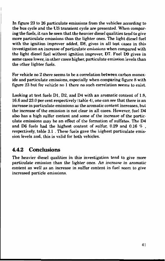
In figure 23 to 26 particulate emissions from the vehicles according tothe bus cycle and the US transient cycle are presented. When compar-ing the fuels, it can be seen that the heavier diesel qualities tend to givemore particulate emissions than the lighter ones. The light diesel fuelwith the ignition improver added, D8, gives in all test cases in thisinvestigation an increase of particulate emissions when compared withthe light diesel fuel without ignition improver, D7. Fuel D9 gives insome cases lower, in other cases higher, particulate emission levels thanthe other lighter fuels.

For vehicle no 2 there seems to be a correlation between carbon monox-ide and particulate emissions, especially when comparing figure 8 withfigure 23 but for vehicle no 1 there no such correlation seems to exist.

Looking at test fuels Dl, D2, and D4 with an aromatic content of 1.8,16.6 and 23.0 per cent respectively (table 4), one can see that there is anincrease in particulate emissions as the aromatic content increases, butthe increase of the emission is not clear in all cases. However, fuel D4also has a high sulfur content and some of the increase of the partic-ulate emissions may be an effect of the formation of sulfates. The D4and D6 fuels had the highest content of sulfur, 0.29 and 0.16 % ,respectively, table 3.1 . These fuels gave the highest particulate emis-sion levels and, this is valid for both vehicles.

4.4.2 ConclusionsThe heavier diesel qualities in this investigation tend to give moreparticulate emission than the lighter ones. An increase in aromaticcontent as well as an increase in sulfur content in fuel seem to giveincreased particle emissions.

41

3.S -

3 -

2 5 -

2 -

1.5 -

I -

OS -

02 0 4 D5 OB

Figure 5. CO emissions, in g/km, vehicle 1, mean value and standarddeviation, bus cycle.

2 6

20

2 4

2.2

2

1.6

1.0

1.4

1.2

1

0 8

0.9

0 4

0 2

OD2 D4 D5 0 9

Figure fi. CO emissions, in |{/km, vehicle I. mean value and standarddeviation, ITS transient cvcle.

42

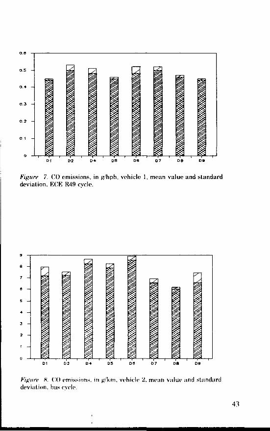
0.5 -

0.3 -

0.5 -

0.1 -

Dl D2 D4 DS DS D7 08 D9

Figure 7. CO emissions, in g/hph, vehicle I, mean value and standarddeviation, ECE R49 cvcle.

9

6 -

7 —

6 -

S -

4 -

3 -

2 -

1 -

001 04 05 DB 09

Figure H. (X) emissions, in g/km, vehicle 2, me;in Vitlue and standarddeviation, hus cvcle.

43

Figure .9. CO emissions, in g/km, vehicle 2, mean value and standarddeviation, US transient cycle.

2 4

2.2 -

2 -

16 -

1.6 -

1,4 -

1.2 -

1 -

0 8 -

OS -

0 4 -

0 2 -

O -01 DB

Figure 10. CO emissions, in g/hph, vehicle 2, me;m value anrl standarddeviation, KCK R49 cycle.

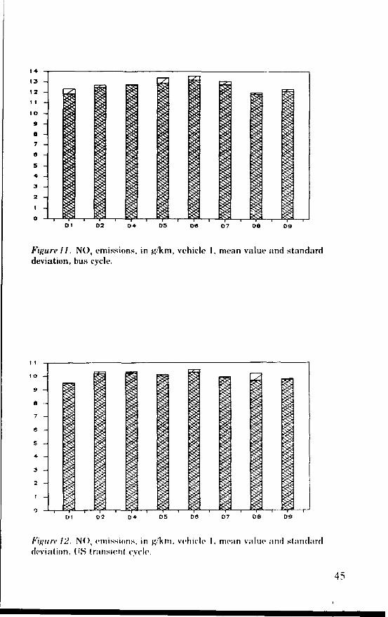
1*

13 -

12 -

1 1 -

10 -

a -7 -

0 -

s -4 -

3 -

2 -

1 -

OD5 D7

Figure 11. NO, emissions, in tf/km, vehicle 1, mean value and standarddeviation, bus cycle.

11

10 -

9 -

6

7 -

8 -

S -

4 -

3 -

2 -

t -

0

FiHtire 12. NO, emissions, in g/km, vehicle 1, mean value and standarddeviation, (IS transient cycle.

2 -

D l OS 0 9

Figure I'.i. NO, emissions, in g/hph, vehicle 1, moan value and standarddeviation, ECE R49 cycle.

161716151413121 110987

es•3210

i

ii

— i —

i

i

01 04 07

Figure 14. N(\ emissions, in g/km, vehicle 2, mean value and standarddeviation, hus cycle.

14

13 -

12 -

1 1 -

10 -

9 -

e

* -5 -

4 -

3 -

5 -

1 -

O0 2 0 4 DS D9

Figure 15. NO, emissions, in g/km, vehicle 2, mean value and standarddeviati. n, US transient cycle.

9

a

7 -

8 -

S -

4 -

3 -

a -

0 2 0 5 0 0 0 7

Figure 16. N()v emissions, in fc/hph, vehicle 2, mean value and standard devia-tion, KCK R4f> cycle.

47

Dl D7 oa D 9

Figure 17. HC emissions, in g/km, vehicle I, mean value and standarddeviation, bus cycle.

I 2

I I -

t —

O 9 -

0 8 -

0 7 -

o e -

0 5 -

o + -

O 3

0 2 -

0 1 -

o

IS. H(' emissions, in tf/km, vehicle 1, mc;in value and standarddeviation, I'.S transient cycle.

48

0.4-S - -

0.4 -

O35 -

03 -

0.25 -

0.2 -

0 15 -

0.1 -

O.OS -

Figure 19. HC emissions, in g/hph, vehicle 1. mean value and standarddeviation, ECK R49 cvcle.

.7

.6

.5

.4

.3

2

1

1

0 9

0 6

0.7

0.9

OS

0 4

0 3

0,2

0.1

0

D1 0 2

20. IIC emissions, in tf/km, vehicle 2. mean value and standarddeviation, hus cvcle.

49

1.3 - -

1.2 -

I.I -

t -

0 9 -

O fl -

0.7 -

o.e -

os -

o • -

0.3 -

0.2 -0.1 -

o - -0 4 DS D8 D9

Figure 21. HC emissions, in g/km, vehicle 2, mean value and standarddeviation, US transient cycle, D6 was not analysed.

0.34

032

0.3

0.26

028

0.24

0.22

0 2

o.i eo.i a0.1 40.1 20.1

0 OS006

0 04

002

0D7

Figure22. HC emissions, in g/hph, vehicle 2, mean value arid standarddeviation, KCK R49 cycle.

oeo

0 30 -

Dl D2 D4 D5 07 DB 0 9

Figure23. Particulate emissions, in g/km, vehicle I, mean value and .standarddeviation, bus cycle.

0.4S

0 4 -

035 -

0 3 -

O 2S -

0 2 -

0 1 5 -

0 1 -

005 -

Dl 0 2 D5 07 DB

Figure24. Particulate emissions, in g/km, vehicle 1, mean value and standarddeviation, US transient cycle.

51

o e -

o 5 -

O 3 -

oe

Figure 25. Particulate emissions, in g/km, vehicle 2, mean value and standarddeviation, bus cycle.

OS

0.4S -

0 4 -

O3S -

0 3 -

o.as -

os -

0 15 -

O 1 -

OOS -

0D2 0 7 DB D 9

Fifiiirv 2(i. Parficulate emissions, in jj/km, vehicle 2. mean value and standarddeviation, US transient cvcle.

52

5 Unregulated Exhaust Emissions

A large part of automotive emissions is not regulated by law. There are.therefore, no requirements to measure other emission components thanthose which are regulated. However, a more thorough characterizationof the emissions requires measurement of specific components. In thisinvestigation, we have concentrated the measurements to such compo-nents as aldehydes, analysis of the particles, olefins. oxygenates andlight aromatics. poly cyclic aromatic compounds and carbon dioxide. InSweden there is a requirement to carry out smoke measurements ondiesel fueled engines in accordance with the method used in this in-vestigation. The results of the measurements have been presented inthis part of the report.

In addition to the chemical characterization of the different emissioncomponents, extracts of samples have been tested using the Amesmutagenicity tests in Salmonella typhimurium and a TCDD dioxinreceptor affinity test.

5.1 ALDEHYDESKerstin GräggEnvironmental SectionSwedish Motor Vehicle Inspection CompanyBox 508, S-162 15 VÄLLINGBY, SWEDEN

5.1.1 IntroductionAldehydes occur in diesel exhaust gases as a result of incompletecombustion, more or less depending on the engine concept and fuelused. Kspecially when using alcohol fuels, there is a large emission ofaldehydes. Aldehydes are irritants to mucous membranes and they areknown to give allergenic reactions and formaldehyde is considered to bea carcinogen iKgeback and Bertilsson, 1983).

5.1.2 Materials and MethodsA chemisorption technique was used for sampling of aldehydes andketones ((Irigoriadis et al. 1987). This method is based on organiccarhonyl compounds reacting with 2,4 dinitro phenyl hydrazine(I)NI'H) at low pH forming corresponding hydrnzones. This techniquehave hern used in several investigations (Westerholm vt »I. 19H6,Björkman ;tnd Kgoback. 1987. (Viporiadis et al. 1987». Brown glass

tubes (160 x 9 mm ID) are packed with Dowex (Dowex 50 H+ Wx4100-200 mesh, Serva, FRG), an ion exchange resin, and further theDowex matrix was coated with 2,4 DNPH. Up stream the DNPH-coatedresin there is a bed of uncoated resin which will reduce the background.Prior to sampling the tubes were cleaned with newly distilled tolueneand dried under a gentle stream of nitrogen. To prevent the tubes fromcontamination they were stored in solid carbon dioxide until use. Justbefore sampling, the tubes were allowed to achieve room temperature.In order to collect aldehydes, a part of the diluted exhaust was drawnfrom the dilution tunnel through an aldehyde sampling cartridge. Aftersampling, the tubes were sealed and stored in dry ice until extractionand chemical analysis were to be performed. Before the analysis, thesampling tubes are extracted with distilled toluene which will eluteformed hydrazones. The hydrazone derivatives are then analysed withHigh Performance Liquid Chromatography (HPLC) with UV-detection.Quantitation was made with corresponding hydrazone as externalstandard.

5.1.3 Results and DiscussionsTwo samples from each vehicle in combination with each of the eightfuels were collected. However, for vehicle No 2 and fuel D2 only onesample was analyzed. All samples analyzed originates only from thetransient driving cycle named the bus cycle, see chapter 3.3. In figures27 to 30, the results of the aldehyde analyses are presented. Figure 27,formaldehyde and figure 28, acetaldehyde emissions, vehicle 1, meanvalues and standard deviation.

From the figures it can be seen that fuel D7 gives the highest formalde-hyde emission levels and also the highest sum of formaldehyde andacetaldehyde among the tested fuels. Fuels D4, D6 and D9 in combina-tion with vehicle 1 and fuels Dl, D2, D8 and D9 in combination withvehicle 2 gave low emission levels of formaldehyde. Publiched data(Westerholm et. al 1986) which originates from the bus cycle and acommercial diesel fuel showed the following emission factors: formalde-hyde 147+6 mg/km, acetaldehyde 37±6 mg/km. When compared withthe values in table 5.1 it can be seen that for vehicle 1 formaldehydeemission levels is lower, except for fuel D7, where the level is higher.Corresponding emissions from vehicle 2 are generally lower. Regardingacetaldehyde emissions: Vehicle 1; fuels D4 and D6 give lower emissionlevels and D8 higher. Vehicle 2; fuels Dl, D2 and D4 gives loweremission values, but all other fuels higher values of aldehydes than in

54

the above mentioned engine/fuel combinations. Noticeable is that therelation between formaldehyde and acetaldehyde seems to show a high-er ievel of emissions of acetaldehyde for vehicle 2 fuels D8 and D9.According to our experience, the ratio between emissions of formalde-hyde and acetaldehyde is, that the emission level of formaldehyde iscommonly much higher than that of acetaldehyde emissions.

5.1.4 ConclusionsSince only two samples were analyzed from each combination of vehi-cles and fuels and the differences between the results of the two sam-ples is large in 4 to 5 cases, it is difficult to draw firm conclusions. I* isnotable that emissions of formaldehyde and acetaldehyde were on thehighest level for both vehicles in combination with fuel D7, the com-mercial light diesel fuel. An earlier investigation (Björkman and Ege-bäck 1987) showed somewhat lower values for light diesel fuels than forheavier diesel fuels. On the other hand it must be underlined that theremay be differences between different blends of light diesel fuels, espe-cially as no firm standards so far have been set up for light diesel fuelsin Sweden. The results obtained in this investigation call for morestudies to fully understand the nature of the formation of aldehydesduring the combustion process and the connection between the emis-sion of aldehydes and the composition of diesel fuels. Comparing for-maldehyde plus acetaldehyde emission values with HC emission val-ues, the aldehyde contribution is in the range of 7-23 7c that of the HCemission.

5.1.5 ReferencesBjörkman E. and Egebäck K-E. (1987) Påverkar Dieselbränslets Samman-sättning Emissionen ? SNV Rapport 3302

Egebäck K-E. and Bertilsson B-M. (1983) Chemical and Biological Character-ization of Exhaust Emissions from Vehicles Fueled with Gasoline, Alcohol,LPG and Diesel. National Swedish Environmental Protection Board. SNV PM1635, Stockholm

Grigoriadis V, Egebäck K-E., Westerholm R., AlabergT., Strandell M., From-melin Å. and Winquist L. (1987) Chemical Analysis and Biological Testing ofEmissions from a Lean Burn Engine. National Swedish Environmental Pro-tection Board. SNV PM 3222, Stockholm

Westerholm R., AlsbergT, Strandell M., Frommelin Å., Grigoriadis V, Hant-zaridou A., Maitm (»., Winquist L., Rannug U., Egebäck K-E. and Bertilsson T.(1986) Chemical Analysis and Biological Testing of Emissions from a HeavyDuty Diesel Truck With and Without Two Different Participate Traps SAEPaper 860014

55

D7 DS D9

Figure 27. Formaldehyde emissions, in g/km, vehicle 1, mean value andstandard deviation, bus cycle.

0.1

0.09 -

ooa -

007 -

006 -

0.05 -

0.04 -

003 -

002 -

001 -

O

ImD7

Figure28. Acetaldehyde emissions, in g/km, vehicle 1, mean value andstandard deviation, bus cycle.

D9

Figure 29. Formaldehyde emissions, in g/km, vehicle 2, mean value andstandard deviation, bus cycle.

0.17

o.ie0.15

0.1 4

0.13

0.12

0.1 1

0.1

0.09

o.oa

0.070.06o.os0.04

003

002

0.01

00 4 D5 D7

Figure 30. Acetaldehyde emissions, in g/km, vehicle 2, mean value andstandard deviation, bus cycle.

57

5.2 PARTICULATE ANALYSIS ANDSMOKE TEST

Kerstin GräggEnvironmental SectionSwedish Motor Vehicle Inspection CompanyBox 508, S-162 15 VÄLLINGBY, SWEDEN

5.2.1 IntroductionSpecial analyses of the particles were carried out at Ricardo ConsultingEngineers, England. The analyzed components are soluble organic frac-tion (SOF), divided into fuel-derived and oil-derived hydrocarbons, sul-fate and sulfate bound water, carbon, nitrate, phosphate, calcium, mag-nesium, iron and zinc.

5.2.2 Materials and MethodsIn order to analyze the components of the particles, a glassfibre filterwithout teflon coating was used, for vehicle 1: Gelman A-E, and forvehicle 2: Whatman GF/A. The filters were conditioned and weighed inthe same way as the filters described in chapter 3.3. Samples weretaken during the bus cycle driving schedule, three repeated tests wasperformed for each fuel and vehicle. The method used for characterizingdiesel particulate hydrocarbons consists of loading a portion of a partic-ulate-laden filter directly into a suitably modified gas chromatographicinjector. Hydrocarbons are vaporized in this solid sample injection sys-tem and subsequently injected on to a gas chromatography column.Using such a technique, diesel fuel constituents can be resolved fromengine lubricating oil constituents. By this it is possible to resolveparticulate-bound hydrocarbons into those fractions derived from un-burned fuel and those originating from unburned lubricating oil. Themethod is described in more detail elsewhere (Cuthbertson and Shore,1987).

For analyzing the carbon content of the particles a thermogravimetricmethod has been used. The particulate sample is heated in a thermobalance to remove volatile material. When a stable weight is achieved,air is introduced and carbon is oxidized, the weight loss monitored isused to obtain the mass of carbon.

58

Sulfate, sodium, potassium, calcium magnesium nitrate and phosphateare measured using ion chromatography. Sulfate bound water is acalculated value. The ion chromatography was also used for iron andzinc, following post-column reaction to form coloured complexes.

5.2.3 Results and DiscussionsSoluble organic fractionThe mean values of the soluble organic fraction, divided into fuel-derived and oil-derived hydrocarbons are presented in and figures 31and 32.

The same synthetic lubrication oil (Mobil Delvac 1) was used through-out this investigation for both vehicles. Therefore it should be possibleto study the influence of the fuels on the particles. Again, \4 .st bepointed out that the two engines of the vehicles are different. In gener-al, the engine related emission level is, therefore, not a relevant param-eter to be compared except when comparing the ratio between the oil-and the fuel-derived part of the soluble organic fraction (SOF) Theoil-derived part of SOF for particles emitted from vehicle 1 is higherthan particles emitted from vehicle 2. Also, when looking at the sum ofthe mass of the oil-derived and fuel-derived fractions, it is obvious thatthe emission level of SOF is higher for vehicle 1 than for vehicle 2. Itshould be noted that the total mass flow rate of particulate emission islower for vehicle 1 than for vehicle 2.

When comparing different parameters it can be seen that, for vehicle 1the final boiling point (FBP) and the fuel-derived hydrocarbons corre-spond very well to each other, but for vehicle 2 not so well. For bothvehicles fuel D6, which has the highest end boiling point, has thehighest mass of fuel derived hydrocarbons, see figures 31 and 32.

The oil-derived part of SOF varies much more from one fuel to anotherfor vehicle 1 than for vehicle 2. However, no such variation of theoil-derived part of the SOF of the particles was expected when using thesame vehicle and the same lube oil which only varying the fuels. As aresults of these findings, further investigations are needed to fullyunderstand nature of the emission of SOF.

Sulfates and sulfate bound waterThe soluble sulfate part of the particles from both vehicles fueled withthe D4, D5, D6 and D7 were analysed and the part of sulfate boundwater was calculated. At 50% relative humidity the sulfates bind waterto about 1.3 times their own weight. The results of the sulfate analysesare shown in figures 33 and 36.

59

From figure 33 and figure 35, it can be seen that fuel D4 which has thehighest sulfur content. 0.29 wt-'i, also produces the largest sulfatefraction of the mass of the particle. Fuel D6, with 0.16 wt- 7i sulfur,show a similar result. Taking into consideration the impact of thesulfate parameter, D4 is the fuel that differs significantly from theother fuels with respect to the sulfate part of the particle. The variationof sulfate emission with fuel D6 fuel is great, but there is still a cleartendency towards higher sulfate content of the particles from highsulfur fuel as expected.

Carbon content of the particlesThe carbon content of the particles is presented in figures 37 and 38Concerning vehicle 1, the carbon contents variates between 3T7( to53r/i carbon. Corresponding values for vehicle 2 are 63 7< to 75% car-bon. The formation of carbon particles is a result of incomplete combus-tion of fuel droplets and it depends, therefore, on the engine and theengine fuel injection system.

Nitrate, calcium, magnesium, iron, zinc and phosphateanalysisIn figures 39 and 40, the result of analyses of nitrate in the particles arepresented. Nitrate in the particles was measured in the range of 0mg/km to 3.2 mg/km when vehicle 1 was used and in the range of 0.8mg/km to 3.8 mg/km when vehicle 2 was used. Fuel D4 gave the highestlevel of nitrate. Note that fuel D8, to which 2-ethyl hexyl nitrate wasadded, did not give more nitrate in the particles than D7. No phosphatewas detected in the particles.

No emissions of calcium, magnesium, iron or zinc was found in theparticles originating from vehicle 2. The following emission valuesfrom vehicle 1 was found:

fuel Dl: 13.9 mg/km calcium, 5.0 mg/km magnesium, 20.4 mg/kmiron and 45.8 mg/km zinc , which was about \77< of the mass of theparticles;fuel D2: 7.1 mg/km iron;fuel D7 and D8: 9.9 and 6.2 mg /km zinc, respectively.

In the rest of the test cases these metals were not found. It is verydifficult to interpret these results. One should keep in mind that "mac-ro" particles occasionally may cause large amounts of metals to bepresent in the particles.

60

Smoke testThe smoke test is a test of the visible pollutants from an engine whichis a standard in Sweden for diesel fueled vehicles. The smoke test isperformed as a smoke density test of the exhaust gases produced by theengine. The smoke meter consists of a piston pump, a filter, a samplingpipe and an opto-electrical instrument. The blackening of the filterwhen a certain sample volume of the exhaust gases has been drawnthrough the filter is measured. Only the black or the dark parts of thesmoke will be measured with this method. A Bosch meter was used andthe results of the measuring are presented as Bosch units.

The smoke tests were performed at full load and at a speed of 75 percent of rated speed of the engine for each vehicle, for vehicle 1, 1350rpm and for vehicle 2. 1540 rpm. Vehicle 1 produced only smallamounts of visible smoke. The measured Bosch values were in thelowest part of the measuring range and the blackening was hardlymeasurable. Only a few tests, therefore, will be presented here. All thefuels were tested in combination with vehicle 2, which had producedmore visible smoke. The test results are presented in table 7.

Table 7. Smoke tests

•'uel

D1D2D41)5Dfi1)71)81)9

n;i not analyzed

Vehicle 1Bosch unit:

na'nanao:(().:{

nana

0.7

Vehicle 2Bosch

12

I1111

unit:

M0

•I

.:(

,~>

i.!)

Conclusions from the smoke test are that the level of smoke emission isvery low in almost all cases.

5.2.5 ReferencesCuthherlson, K. I), and Shore, P. H. ll!»H7) Direct Capillary (las Chromatog-raphy of Kilter Borne ('articulate Emissions from Diesel Kugines. -Journal ofChromatographic Science, Volume 2H 11988» Pages I OH 112

(Iregoriadis V.. Kgebiick K-K., Westerholm K., AlsnergT., Strandcll M., Krom-mclin A. and Wmcjuist L. (l!)H7i Chemical Analysis and Biological Testing ofEmissions from a Lean Murn Engine. National Swedish Environmental Hoard,Report .T225, Solna.

tao170 -ieo -150 -1*0 -130 -120 -110 -1O0 -»o -AO -

70 -

60 -

50 -

•»O -

30 -

20 -

10 -

O

y

fuel-der i ved. o i 1-derived

Dl D2 O* DS DU D7 06 09

Figure 31. Soluble organic fraction, in mg/km, vehicle 1, mean values of fuel-derived and oil-derived hydrocarbons of the mass of the particles, bus cycle.

90

SO -

70 -

60 -

50 -

40 -

30 -

20 -

to -

0

Cue 1-dcr i veil o i i -der i ved

01 02 0* DS DÖ 07 DS 09

Fitiun>:i2. Soluble organic fraction, in mg/km, vehicle 2, mean values of fuelderived and oil-derived hydrocarbon.s of the mass of the particles, bus cycle.

so26 -

26 -

24- -

22 -20 -IB -te -I 4- -

12 -

1O -

a -6 -• -

2 -O

01 D2

Figure 33. Soluble sulfates, in mg/km, vehicle 1, mean value and standarddeviation, bus cycle. D1,D2 and D8,D9 were not analysed.

40

35 -

30 -

2S -

20 -

IS -

1O -

5 -

D2 D4 DS

Figure 34. Sulfate bound water, in mg/km, vehicle 1, mean value and standarddeviation, bus cycle. D1.D2 and D8,D9 were not analysed.

Figure 35. Soluble sulfates, in mg/km, vehicle 2, mean value and standarddeviation, bus cycle. D1,D2 and D8,D9 were not analysed.

24

22 -

20 -

16 -

16 -

14 -

12 -

10 -

6 -

6 -

4 -

2 -

00 1 D2 D 4 0 5 D7 0 6 D9

Figure36. Sulfate bound water, in mg/km, vehicle 2, mean value and standarddeviation, bus cycle. D1.D2 and D8.D9 were not analysed.

032

O 3

0.28

0 20

0 2*

0 22

0.2

o.ta

O.It

O.I*

0 12

C.I

ooaooe0.04

0.02o

Dt D2 D4 OS 06 D7 D8 D9

Figure 37. Particle carbon content, in g/km, vehicle 1, mean value andstandard deviation, bus cycle.

0.45

0 4 -

0 35 -

0 3 -

O 2S -

0 2 -

0 15 -

0 1 -

O OS -

III

06 oa

Figure.18. Particle carbon content, in g/km, vehicle 2, mean value andstandard deviation, bus cvcle.

+.5 -

• -

3-S -

3 -

2.S -

a -

1.5 -

1 -

OS -

O -0 5 0 7

Figure 39. Nitrate in the particles, in mg/km, vehicle 1, mean value andstandard deviation, bus cycle. D8 was not analysed.

0 1

Figure 40. Nitrate in the particles, in m^/km, vehicle '2, mean value and.standard deviation, bus cycle.

5.3 OLEFINES

Jacob Almén and Roger WesterholmDepartment of Analytical ChemistryStockholm UniversityS-106 91 STOCKHOLM, SWEDEN

5.3.1 IntroductionIn recent years much effort has been made to characterize the volatilefraction of vehicle exhaust emissions, both oxygenated compounds aswell as non-methane hydrocarbon compounds (NMHC), because of po-tential photochemical smog formation in city areas < Persson and Al-mén, 1990). It is considered that some of these NMHC in urban air canincrease the genotoxic risk for man. Alkenes such as ethene and pro-pene are converted by metabolism in the human body to correspondingepoxide which can react with DNA molecules in the cells and thusinitiate a mutagenic effect. However, ethene is also suspected to becarcinogenic to man (Törnkvist et al. 1988) and, therefore, it is ofimportance to limit emission and exposure.

5.3.2 Material and MethodsThe method used for determination of ethene and propene in thisinvestigation was originally developed and evaluated for urban airmeasurements and this is described elsewhere (Persson and Berg,1989). Sampling and analysis of olefines was accomplished by using agas chromatograph (GC MINI 3, Shimadzu Corp, Japan) equipped witha specially laboratory made injection valve, trap and desorption unit.Samples were drawn from the dilution tunnel into Tedlar bags (10L)during the whole driving cycle. A known volume (range 300 mL) waspumped and trapped onto a solid sorbent (Molecular Sieves 13X, 40-60mesh; Alltech Inc, USA). The sample was then heat desorbed onto thecolumn (stainless steel, 5m x 2mm i.d.) packed with activated alumina(80-100 mesh, Alltech Inc, USA) which was kept at I60"C. For detec-tion, a flame ionization detector (FID) was used. Ethene and propenestandards (Alfax AB, Malmö, Sweden) were diluted with air to anappropriate concentration. External standard calibration methodologywas used and peak integration was carried out by using an integrator(HP 3302, Hewlet Packard Inc, USA). Blank samples from the dilutiontunnel were taken daily with the vehicle disconnected from the dilutiontunnel.

f>7

Prior to this investigation, decomposition of ethene and propene, due toexposure to high concentrations of NG\, was studied. Tedlar bags withexhaust emissions were analysed after 8 h time period for two days. Nosignificant changes was detected i.e. less than 5 % imply that storagewas consided not to have a major impact on the analysis results pre-sented. Chemical analysis was, in all cases performed the same day assampling of exhaust emissions.

5.3.3 Results and DiscussionsIn figures 41 to 44, the emission results of measured olefins are present-ed originating from the bus cycle driving conditions.

Vehicle one:From the figure 41, it can be seen that mean ethene emissions from thefuels investigated i.e. fuels D4 to D9 are in the range 30 to 40 mg/km.Fuel D4 giving the lowest and fuel D8 the highest emission values.Comparing the results presented with published values (Grägg et al.1989) a factor of two times lower emissions was measured in thepresent study. Propene emissions presented in figure 42 range from 7 to12 mg/km. The largest emission values originate from fuel D7 and thelowest from fuel D8. However, this implies that addition of ignitionimprover decreases emissions of propene.

Vehicle two:Ethene emissions are presented in figure 43 from which it can be seenthat the emission variates between 60 to 140 mg/km which is in accord-ance with previously reported emission values originating from aheavy-duty diesel truck (Grägg et al. 1989) and from a light-duty die.selvehicle (Egebäck and Bertilsson, 1983). The highest emission levelswere measured with fuels D5, D6 and D7. Addition of ignition improverreduced the emission of ethene by a factor of approximately two com-paring fuels D7 and D8. Emissions of propene are displayed in figure44. In the figure the emissions mean values variates between 7 and 20mg/km. Low emission values were obtained from fuel D4 and D6 re-spectively compared to fuels D7 and D9 which produced the highestvalues of propene. From the figure it can also be seen that addition ofignition improver reduces emissions of propene. However, fuel 1)7 showa large standard deviation. Emission Vd'.'jps are in the same order asreported by Grägg and co-workers (Grägg et al. 1989).

68

5.3.4 ConclusionsEthene and propene emissions are fuel dependent. However, wherethere is an addition of 2-ethylhexyl nitrate to the fuel a reduction ofethene and propene emissions is indicated. The range for ethene emis-sions are 30 to 140 mg/km. Corresponding propene emission factors arein the range 5 to 20 mg/km.

5.3.5 ReferencesEgebäck K.E and Bertilsson B-M. (1983) Chemical and Biological Character-ization of Exhaust Emissions from Vehicles Fueled with Gasoline, Alcohol,LPG and Diesel. National Swedish Environment Protection Board, SNV PM1635, Solna.

Grägg K., Lundström L., Egebäck K.E. (1989) Investigation of two HeavyDuty Diese1 Particulate Traps. National Swedish Environment ProtectionBoard, SNV Report 3577, Solna, in Swedish.

Persson K-A and Berg S. (1989) Automatic Determination of Selected C2-C4Hydrocarbons in Urban Air by Solid Sorbent Sampling and Gas Chromatog-raphy, Chromatographia, 27 55.

Persson K-A. and Almén J. (1990) Characterization of Light Hydrocarbons andOther Volatile Organic Compounds in Stockholm Air. National Swedish Envi-ronment Protection Agency, Report 3820, Solna,

Törnqvist M., Kautiainen A., Gatz R-N. and Ehrenberg L. (1988) HemoglobinAdducts in Animals Exposed to Gasoline and Diesel Exhaust J. Appl. Toxicol.8, 159-170

69

50

45 -

+0 -

35 -

30 -

25 -

:o -

15 -

1 0 -

5 -

002 D7

Figure 41. Ethylene emissions, in mg/km, vehicle 1, mean value andstandard deviation, bus cycle, Dl and D2 were not analysed.

13

12

1 1

1 O

9

e

7

es

3 -

2 -

1 -

OD1 0 4 D5 0 7

Figure 42. Propylene emissions, in mg/km, vehicle 1, mean volue andstandard deviation, bus cycle, Dl and D2 were not analysed.

70

150

14-0

130

120

1 10

100

SO

SO

70

eo50

40

30

20

1 0

001 D2 05 07 08

Figure 43. Ethylene emissions, in mg/km, vehicle 2, mean value andstandard deviation, bus cvcle.

30 -

20 -

Figure ii. Propylene emissions, in mg/km, vehicle 2, mean value andstandard deviation, hus cvcle.

71

5.4 OXYGENATED AND LIGHT AROMATICCOMPOUNDS

Jacob Almén and Roger WesterholmDepartment of Analytical ChemistryStockholm UniversityS-106 91 STOCKHOLM, SWEDEN

5.4.1 IntroductionA large number of alifatic, olefinic, cyclic and aromatic oxygenates hasbeen identified in the exhaust emissions from both gasoline and diesel-fueled vehicles (Jonsson et al. 1985). Some of them are suspected asbeing carcinogenic to man (Lutz and Schlatter,1977). Other effects,associated with oxygenated hydrocarbons are irritation of eyes andmucous membranes (Altshuller,1978). Exhaust emissions from trafficare the most important antropogenic source of aldehydes and otheroxygenates in ambient air, both directly and through secondary forma-tion via photochemical reactions of emitted hydrocarbons (Persson andAlmén,1990). On account of their possible detrimental effects onhealth, emission of oxygenates and light aromatics must be reduced invehicle exhaust emissions

5.4.2 Materials and MethodsSampling of oxygenates and light aromatics was accomplished using acryogenic sampling technique (Jonsson and Berg 1983) in which acryogradient is established over a sampling tube packed with a sorbentbed. the cryogradient sampling tubes were made of pyrex glass tubing(380 mm x 3 mm I.D.). The sorbent material (Chromosorb WAW, 30-60mesh, Jonhs-Manville, USA) was deactivated with 3,3,3-trifluoropro-pyl methyl cyclotrisiloxane and coated with 5% of SP-2401 (SupelcoINC, USA). Prior to sampling the adsorbant tubes were conditionedover night under a stream of nitrogen at 180°C. The cryogradientsampling device (AMA PN; AMA, FRG) was modifieu according toJonsson and Berg (Jonsson and Berg 1983) with a heating wire duringsampling to establish a gradient from -50 to -150°C. The cryogradientsampling equipment was connected to the dilution tunnel with a fluorocarbon probe which was heated to 105 °C to prevent condensation ofwater. One sample was collected for each driving cycle. After sampling,the tubes were sealed and stored in a vessel containing dry ice and

72

transported to the laboratory for analysis. Blank samples were takenwithout vehicles connected to the dilution tunnel and then analysed.Analysis of oxygenates and light aromatics were achieved with a two-dimensional gas chromatograph which is described in detail elsewhere(Berg and Jonsson 1984).

5.4.3 Results and DiscussionsThe emissions of oxygenates i.e. acroleine, methacroleine are presentedin figures 45 to 48, other oxygenates measured but not presented in thispresent report will be tabulated elsewhere (Westerholm and Egebäck,1991a). Comparing the emission factors in the figures with those previ-ously reported by Jonson and co-workers (Jonsson et al. 1985), it can beseen that the emission factors are approximately 20 to 50 per cent lowerin this current investigation. However, another investigation (West-erholm et al. 1991) gives results similar to those presented in figures 45to 48.

Vehicle 1:

Acroleine and methacroleine emissions values are lowest from fuel D4and the highest emissions measured originate from fuel Dl, (figures 45and 47). Range for acroleine is approximately 8 to 18 mg/km and formethacroleine approximately 2 to 3 mg/km. The other fuel qualitiesgave intermediate emission values. Emissions of benzene and tolueneare shown in figures 49 and figure 51 respectively. The highest emis-sion levels measured originate from fuel Dl. However, only a singleanalysis was performed why no standard deviation was obtained. Thelowest emission levels were detected in the exhaust when fuels D7 andD8 were used. The span is roughly 4 to 8 mg/km for benzene and fortoluene the corresponding values are 2 to 9 mg/km.

Vehicle 2:Both acroleine and methacroleine emissions are presented in figures 46and 48 are relatively fuel independent. However, methacroleine emis-sions was reduced by approximately 25% when using diesel ignitionimprover i.e. fuel D8. Ranges measured for acroleine were 25 to 35mg/km and for methacrolein 4-5 mg/km. In the bar chart figures 50and 52 are benzene and toluene emission factors are displayed, respec-tively. The highest emission levels were obtained from fue) D6, valid forboth benzene and toluene, 13 mg/km. The other fuels investigated gave

73

similar lower emission values compared to D6. The lower range is forbenzene 8 to 10 mg/km and for toluene 4 to 6 mg/km, respectively. Aslight emission reduction of benzene and toluene was measured whenadding diesel ignition improver to fuel D7.

Comparing benzene and toluene emissions magnitudes with publisheddata (Westerholm et al. 1991, Jonsson et al. 1985) it can be seen thatsimilar results are obtained in this present investigation.

Using the sampling and analysis technique developed by Berg andJonsson (Berg and Jonsson, 1984), it was also possible to measureethylacetate emissions from heavy-duty diesel vehicles. Emission fac-tors of ethylacetate have not, to our knowledge, previously been report-ed from heavy-duty diesel vehicles. Emission factors of ethylacetatefrom both vehicles after blank corrections were in the range of 0.15 to0.4 mg/km. However, confirmation of ethylacetate has been carried outwith retention time from reference substance only.

5.4.4 ConclusionsThe lowest emission rate of acrolein was determined to be 8 mg/km andthe highest emission values were 35 mg/km. The lowest emission val-ues of metacrolien were determined to be 2 mg/km and the highestemission values waere 5 mg/km. The lowest emission valuesof benzenewere determined to be 5 mg/km and the highest emission values was 13mg/km. The lowest emission values of toluene were determined to be 2mg/km and the highest emission values were 13 mg/km. Thus, selectionof fuel reduces the emission of oxygenates and light aromatics by afactor of 3 to 6.

The addition of diesel ignition improver had no major impact on theemissions of oxygenates and light aromatics.

5.4.5 ReferencesAltshuller A. (1978) Assessment of the Contribution of Chemical Species to theEye Irritation Potential of Photochemical Smog. J. Air. Pollut. Oontr. Assoc,28, 594-

Berg S. and Jonsson A. (1984) Two-Dimensional (las Chromatography forDetermination of Volatile Compounds in Ambient Air. Journal of High Resolu-tion Chromatography and Chromatogragniphy Communications. Vol. 7,687-695.

74

Jonsson A. and Berg S. (1983) Determination of Low-molecular-weight Ox-ygenated Hydrocarbons in Ambient Air by Cryogradient Sampling and Two-dimensional Gas Chromatography. J.Chromatography, Vol. 279 307-322.

Jonsson A., Persson K-A. and Grigoriadis V. (1985) Measurements of some LowMolecular Weight Oxygenated, Aromatic, and Chlorinated Hydrocarbons inAmbient Air and in Vehicle Emissions. Environment International, Vol. 11,383-392.

Lutz W.K. and Schlatter C.(1977) Mechanism of the Carcinogenic Action ofBenzene: Irreversible Binding to Rat Liver DNA. Chern.-Biol. Interact. 18(2),241-245.

Persson K-A. and Almén J. (1990) Characterization of Hydrocarbons andOther Volatile Organic Compounds in Stockholm Air. Swedish EnvironmentalProtection Agency. SNV PM 3828, Solna.

Westerholm R. and Egebäck K-E. Eds. (1991a) Supplement of data: "Impact ofFuels on Diesel Exhaust Emissions: A chemical and biological character-ization." Swedish Environmental Protection Agency, Report, Solna, in prep-aration.

Westerholm R., Almén J., Li H., Rannug U., Egebäck K-E. and Grägg K.(1991) Chemical and Biological Characterization of Particulate, Semi-volatileand Gas Phase Associated Compounds in Diluted Heavy Duty Diesel Ex-hausts: A comparison of three different semi-volatile phase samplers. Environ.Sci. Technol. 25. 332-338. 1991.

75

1 9ta17161 St 4t 31 2t 11 O

aa

D 2 D-f 05 D7 DB D9

Fiffurv 45. Acrolein emissions, in mg/km, vehicle I. mean value anastandard deviation, bus cycle.

Fifiurv 4(i. Acrolein emissions, in m^/km, vehicle '2, mean value andstandard deviation, hus cycle.

3.2

3 -

28 -

2.6 -

2.4 -

2.2 -

2 -

1.8 -

1.8 -

1.4 -

1.2 -

1 -

OB -

0 8 -

0.4 -

0 2 -

O01 02 04 05 08 07 08 09

Figure47. Methacroicin emissions, in mg/km, vehicle 1, mean value andstandard deviation, bus cycle.

0 1

Figure IH. Methacrolein emissions, in m^/km, vehicle 2, mean value andstandard deviation, hus cycle.

77

Figure 41). Benzene emissions, in mg/km, vehicle 1, mean value andstandard deviation, bus cycle.

16

15

1 4

13

12

1 1

1 0

9

S

7

6

5

4

3

2

1

0D2 0 7 DB

Figure 50. Renzene i-missions, in mg/km, vehicle 2, mean value andstandard deviation, bus cvcle.

78

Figure 51. Toluene emissions, in mg/km, vehicle 1, mean value andstandard standard deviation, bus cycle.

Figure 52. Toluene emissions, in m^/km, vehicle 2, mean value andstandard deviation, bus cycle.

7*)

5.5 POLYCYCUC AROMATIC COMPOUNDS

Hang Li, Elisabeth Hallgren, Lena Elfver andRoger WesterholmDepartment of Analytical ChemistryStockholm UniversityS-106 91 STOCKHOLM, SWEDEN

5.5.1 IntroductionDuring incomplete combustion in air using organic fuels in combustionengines, among other pollutants, polycyclic aromatic compounds (PAC)are formed iRamdal, 1983, Hayano et al. 1985). Of these PAC com-pounds some of them such as benzol a )pyrene, cyclopenta(cd)pyrene areknown to be mutagenic in the salmonella typhimurium bio-assay test(IARC, 1983). Thease PAC belongs to the group of compounds denotedpolycyclic aromatic hydrocarbons (PAH). Another group of compoundsformed are nitro derivatives of PAH such as, for example, nitro-pyrenewhich has an accentuated response in the Ames test compared tocorresponding PAH. (Rosenkranz et al. 1985). Due to the fact that someof the PAC compounds are mutagenic in the Ames test and in somecases also give rise to cancer in animals in skin painting experiments(IARC, 1983), it can be expected that these PAC compounds may havethe adverse effect of causing cancer in humans. Therefore it is impor-tant to reduce the emissions of PAC in vehicle exhaust. An importantfactor affecting the emissions of PAC is the selection of fuel and fuelcomponents (Baines et al. 1982). However, to support a possible in-troduction of standards, it is of importance to obtain more knowledgeregarding the relationship between fuel parameters/components andexhaust emissions of known/suspected mutagenic compounds. One ap-proach to gain such knowledge is to use chemical characterization inconnection with bio-assay tests on exhaust emission samples from mo-tor vehicles.

5.5.2 Materials and MethodsParticulate associated PAC emission samples were collected on Tefloncoated glass fibre filters (Pallflex T60A20, Pallflex INC, USA) accord-ing to specification in U.S. Federal Register (Federal Register 1987).The filters were weighted before and after sampling according to thespecifications in the Federal Register (Federal Register 1987). However,

80

prior to sampling, the filters were washed. The washing procedure isdescribed elsewhere (Westerholm el al. 1988». After sampling, the fil-ters were stored at -20 C until extraction. The filters were Soxhletextracted with dichloromethane for 18 h (170 mL, 20 minutes refluxingtime). All solvents used were distilled in an all-glass column if nothingelse is stated. The crude dichloromethane extract was evapora' ed underreduced pressure, diluted with acetone to a known volume and dividedinto two fractions, one for chemical analysis and one for biologicaltesting, see sections 6.1 and 6.2. Both fractions were then stored at-20 C until chemical analysis/biological testing. Blank was performedas described, however, without the vehicle. The organic soluble fraction(OSF) of the filter samples was measured by weighting the filter sam-ples before and after extraction with dichloromethane.

The semi-volatile phase emission was trapped down streams a PallflexT60A20 filter using polyurethane foam (PUFt plugs. The samplingdevice is made of anodised aluminum. The size of a poly urethane foamplug is: height 50 mm, diameter 70 mm and the density of the materialis 23 g/cm!. The poly-urethane foam plugs were washed before sam-pling which is described in detail elsewhere I Westerholm et al. 1991).The purified polyurethane plugs were stored separately in tight glassjars until sampling. After sampling, the poly urethane plug was trans-ferred to a tightly sealed glass jar and stored at -20 "C until extraction.The samples were Soxhlet extracted with acetone for 12 h. The acetoneextract was evaporated under reduced pressure, diluted with acetone toa known volume and divided into two fractions, one for chemical analy-sis and one for biological testing. Both fractions were then stored at-20 C until chemical analysis/biological testing. Kach PUK-plug wasused only once for sampling.

The participate and the semi-volatile phase crude extracts were frac-tionated according to polarity into three fractions after addition ofinternal standard (2, 2'-binaphtyl>eluting in the PAH fraction. An open(120 mm x 5 mm id.) silica gel column (Merck silica, KK(I, O.OH.'i 0.200mm), was filled silica gel which was deactivated with 10 ", water(WAV), the detail was described elsewhere (Alsberg et al. 1985). Thethree fractions collected were as follows: fraction I, eluted with 4.2 mLof hexane (containing "light" aliphatic hydrocarbons); fraction II, elut-ed with 14.0 mL of hexane ("heavy" aliphatic hydrocarbons, polycyclicaromatic hydrocarbons); fraction III, eluted with 18.0 mL 25 ''•', dichlo-romethane in hexane (nitro polycyclic aromatic hydrocarbons) according to Alsberg and co-workers (Alsberg et al. 1985). However, thesolvent elution volumes were modified to fit the column size.

SI

Since fraction II from the silica gel column contained aliphatic materi-al, it was subjected to further cleaning up using high performanceliquid chromatography (HPLC) according to Östman and Colmsjo (Öst-man and Colmsjö, 1987, Östman and Colmsjö, 1989). The HPLC systemconsisted of a Waters pump unit M45 (Waters INC., USA), connected totwo pneumatically actuated three- and four-port Valco switching-valves controlled by a laboratory data system (Chromatography DataSystems AB, Sweden), hexane is used as mobile phase. The first valvewas used for back-flushing the column, which was packed with 10 /UM/*Bondapak-NR, particles (250 mm, 7.8 mm id. Waters INC., USA) ardused for the separation, the effluent was monitored with a U)C Spec-tromonitor HI (LDC INC, USA) UV detector adjusted to 254 nm. Thecolumn separates primarily according to the number of aromatic ringsin the molecule. Aliphatics, monoaromatics and diaromatics were elut-ed before back flushing the column. In the back flush peak, I'AC withthree or more aromatic rings were eluted. In this way two sub-fractionswere obtained containing aliphatic material and PAC, respectively.

The sub-fraction containing the PAC was analysed using gas chrorna-tography-mass spectrometry (GC-MS). The gas chromatograph usedwas a 5790A (Hewlett-Packard, USA) with a split/splitless injector, afused silica capillary column (15 m x0.22 mm i.d.,CP-sil 8 Chrompack,The Netherlands). The temperature program was: isothermal 70 (' forone minute, increase 7"C/min to 300 C, isothermal .'WO C for 9 min-utes, carrier gas helium. A Jeol D300 mass spectrometer was used (JeolINC, Japan), operated in the electron impact ioni/ation mode. MS-interface temperature 300"C; ion source temperature 200"C; ionizationvoltage 70 eV; scan range 35-1350 amu; scan time 1.0 s. The massspectrometer was interfaced to the Finningan computer system (NCOS2000 (Finnigan INC, USA). Quantitation was made by integration ofthe molecular ions of the internal standard and the PAC. A standardmixture containing known amounts of both internal standard and alldetermined PAC was used for response factor calculations and for deter-mination of retention times.

Analysis of fraction III, originating from both participate and semi-volatile phase with regard to 1-nitro pyrene, was accomplished bymeans of a method developed by Tejada and co-workers which is de-scribed elsewhere (Tejada et al. 1986). The sample is analysed by areversed phase HPLC system, using heart-cutting and on-line reduc-tion of 1-nitro pyrene to 1-amino pyrer.e. This system consisted ofWaters Automated Valve Station (WAVS, Waters INC., USA), a Pro-

82

grammable Solvent Delivery Module (Model 590, Waters INC., USA)and a Shimadzu Fluorescence HPLC Monitor (Shimadzu INC., Japan),which wde controlled by a Gradient Master (Laboratory Data Control,USA). After pre-separation on a Sperisorb 5 C-8 (Phase Sep, USA)column (45 mm x 4.6 mm i.d.), catalytic reduction was executed in acolumn (40 mm x 3 mm i.d.) filled with 5 /u.m alumina particles coatedwith 1.03 7c Platinum/Rhodium 110. The peak corresponding to theretention time of 1-nitro pyrene and the internal standard (benz(a)anthracene, added to fraction III) was switched via two six-port highpressure valves to the analytical column, a Supelcosil LC18-DB 5 /um,150 mm x 4.6 mm i.d. (Supelco INC.,USA). Here, 1-amino pyrene wasseparated from benz(a)anthracene and other substances co-elutingfrom the pre-column. Methanol/water was used as mobile phase, whichduring the pre-separation consisted of 55 7c methanol in water. All runswere gradient-programmed, and the mobile phase composition nomi-nally ranged from 55 7c, 60 7c, 75 V( to 85 7r, during the secondseparation step. Further, oxygen was removed from the n. ">ile phase bya catalyst column (45 mm x 4.6 mm I.D.) situated in . ont of theinjection valve. This column contained traces of nickel, platinum andrhodium on a ceramic support, obtained from finely ground materialfrom an automobile exhaust catalytic converter. The temperature of theoxygen scrubber was held at 70°C. Quantitation was performed byusing the integrated fluorescence signal of 1-amino pyrene with that ofbenz( a »anthracene. For this purpose, the fluorescence detector wasused, at an excitation wavelength of 284 nm and emission wavelengthof 387 nm for benz( a (anthracene, and excitation wavelength of 360 nmand emission wavelength of 430 nm for 1-amino pyrene. A trilab 2000laboratory data system (Trivector Scientific Ltd, UK) was used for dataprocessing.

PAC analysis of the fuels were performed as follows: internal standardwas added (2,2' binaphtyl) to 100 /il fuel and the volume was reducedusing a gentle stream of nitrogen. The residue was dissolved in DKMand transferred to 100 mg deactivated silica gel (10% water) and theDKM solvent was evaporated using a gentle stream of nitrogen. Thesilica gel was put on the top of the silica gel column and the fuel samplewas fractionated in two fractions according to method previously de-scribed for the exhaust PAC. The PAC fraction was further fractionatedwith HPLC according to Östman and Colmsjö (Östman and Colmsjö,1989) and the obtained fraction was analyzed with GC-MS as describedpreviously.

5.5.3 Results and DiscussionsThe organic soluble fractions (OSF) are presented in figures 53 and 54for vehicle one and vehicle two, respectively, and resembles what can beextracted from the carbon matrix from diesel engine generated partic-ulate material which is in the range 10-40 % by weight of the partic-ulate mass (National Research Council 1982). Comparing solubleorganic fraction, analyzed by another laboratory, SOF presented infigures 31 and 32 with OSF figures 53 and 54, it can be seen that valuesof OSF are generally higher.

The individually analyzed PAC were: dibenzothiophene, 4-methyldi-benzothiophene, 3-methyldibenzothiophene, 2-methyl fluorene, phe-nanthrene, anthracene, 3-methyl-phenanthrene, 2-methyl-anthracene,4&9-methyl-phenanthrene, 1-methyl-phenanthrene, fluoranthene, py-rene, retene, benzo(a)fluorene, 2-methyl-pyrene, 1-methyl-pyrene, ben-zol ghi »fluoranthene, cyclopenta(cd)pyrene, benzo(a)anthracene, chry-sene/triphenylene, benzo(b& k (-fluoranthene, benzo(e)pyrene, benzo(a)pyrene, perylene, indeno(l,2,3-cd)fluoranthene, indeno(l,2,3-cd)py-rene, picene, benzofghi(perylene and cornene.

The individual PAC analyzed in fuels, particulate and semi-volatilephases are added together and termed "sum of PAC" when presented infigures. All figures represented by blocks are mean values, the stan-dard deviation being represented by the overlying block on top of themean value. The data given in figures for the particulate phase aremean values from three test runs analyzed separately from each fueland vehicle. However, for the semi-volatile phase the data representone sample from each fuel and vehicle analyzed in triplicate. Blanksamples from the particulate and the semi-volatile phase was analyzedchemically with regard to PAC content. The contribution from theblank samples consisted mainly of phenanthrene, anthracene and theirmono methyl derivatives. Only insignificant traces of 1-nitro pyrenewas detected in the particulate phase. In the semi-volatile phase no1-nitro pyrene was detected.

Each fuel was analyzed in duplicate for PAC contents which are pre-sented in figure 53. The factor on top of block is the multiplicationfactor by whi'h the bar has been multiplied. From the figure it can beseen that fuels Dl, P2 and D4 have low PAC contents; approximately1 4 mg/L compared to the other fuels, fuels D5, D7,1)8 and D9 havinga PAC contents of approximately 200-350 mg/L. Fuel 1)6 has the

84

largest PAC content which is in the range 1100 mg/L. Major contrib-utors to fuel PAC contents are methyl-phenathrenes and methyl-an-thracenes. The multivariate analysis, appendix section, reveals thatfuel PAC is an important variable with respect to correlations fuelvariables to chemical composition and biological effects in the exhaustemissions. Other important fuel variables are distillation 90 7t andfinal boiling point. However, this indicates that fuel PAC are related tofuel components characterized by distillation 90 7t and final boilingpoint.

Vehicle 1:Emissions of polycyclic aromatic hydrocarbons (sum of 29) in the partic-ulate phase are displayed in figure 56. Low emission values weremeasured in the exhaust when using fuels Dl, D2 and D4 which are inthe range 25 45 (ig/km, and intermediary emission values in theexhaust when using fuels D5, D7, D8 and D9 which are in the range75-120 fig/km. The largest emission values were measured when us-ing fuel D6, approximately 220 /xg/km.

Emissions of PAC in the semi-volatile phase are displayed in figure 57.The lowest emission values are detected in emissions from fuels D2, D4and D7, less than 35 /ig/km. Intermediary emissions values of 75-150/Ltg/km originate from fuels Dl, D5, D8 and D9. The largest emissionvalue was measured in the exhaust when using fuel D6 which is in therange 230

Considering both particulate and semi-volatile PAC emissions the low-est emission values, less than 150 /ug/km, were detected in the exhaustwhen using fuels Dl, D2, D4, D7, D8. The highest emission valueoriginates from fuel D6, larger than 300 /ttg/km and intermediate emis-sion values originate from fuels D5 and D9, range 200 to 300 /ng/kin.The best fuels with respect to PAC emissions are fuels D2 and 1)4. Thesemi-volatile phase PAC contribution of the total PAC emissions variesbetween 8 'Y< (D2) and 70 % (Dl) of the total emission.

The 1-nitropyrene emissions are presented in figure 58. Tht> emissionsobtained when using fuels D2, D5, D7, D8 and D9 were less than 0.3/ig/km which is relatively low compared to previous results (Wester-holm et al 1986). When using fuels Dl, D4 and D6 the range is 0.6-1.1yug/km. However, the standard deviation is relatively large. Emissionsdetected in the semi-volatile phase were less than 0.07 /xg/krn for allfuels tested.

85

Vehicle 2:The particulate associated PAC emissions are presented in figure 59.The PAC emission values were lowest when using fuels Dl, D2, D4, D7,approximately 50-80 /xg/km, intermediary, with fuels D5 and D8,90-120 /xg/km, and largest for D6 and D9 in the range 160-170/tig/km. When comparing fuels D7 and D8, no significant difference canbe established although the only difference is that D8 contains anignition improver. This is also valid for vehicle one.

The semi-volatile phase associated PAC emissions are presented infigure 60 from which it can be seen that the lowest emission valueswere obtained when using fuels Dl, D2, D5, D7 and D8 which are in therange of 10-40 /xg/km. Intermediary fuels with regard to these emis-sion components are D4 and D9 being in the range of 70-120 /xg/kmand the highest emission value was detected in the exhaust originatingfrom fuel D6, approximately 200 tig/km.

When comparing the total emission of PAC i.e. both particulate andsemi-volatile phase associated, it reveals that the lowest emission val-ues originates from fuels Dl, D2, D4, D5, D7 and D8, less than 160/xg/km, intermediate, from D9, less than 300 /xg/km, and finally D6more than 300 /xg/km. This result implies that fuel D6 is the mostunfavorable fuel with respect to PAC emissions and fuels Dl and D7best. The per cent contribution from the semi-volatile phase variesbetween 12 % (D7) to 63 % (D4) of the total PAC, which implies theimportance of sampling and analysing the semi-volatile phase PACemissions on account of fuel dependence.

The 1-nitropyrene emissions detected in the particulate phase are dis-played in figure 61. Low emission values of less than 1 /xg/km, aremeasured when using fuels Dl, D7 and D8, intermediate emissionvalues in the range of 1-3 tig/km, in fuels D2, D5, D6 and D9, and thelargest emission values approximately 7 /xg/km, when using fuel D4,although, a very large standard deviation was obtained. The semi-volatile associated 1-nitropyrene was determined to be less than 0.07/xg/km, which is valid for all fuels tested.

Comparing data presented in this present study with published datawhich originates from the bus cycle using a heavy duty truck fueledwith a commercial diesel fuel quality (Westerholm et al. 1991), similarPAC emission rate values were obtained in the particulate phase whichoriginates from fuel D6. The semi-volatile phase PAC emitted from fuel

86

D6 is approximately only a third of the PAC emission measured in anearlier investigation (Westerholm et al 1991). This implies that thePAC emissions measured is strongly fuel and engine concept depend-ent. Regarding the emission of 1-nitro pyrene, about the same magni-tude of emissions are emitted when using the fuels designed for thisstudy as previously reported i.e. 1.6 /ug and <0.05 /xg/km, particulatephase and semi-volatile phase, respectively (Westerholm et al. 1991).However, a relatively large standard deviation was obtained in thisstudy.

PAC present in the semi-volatile phase compared to the particulatephase associated PAC is at most approximately 90 per cent for 2-methylfluorene and phenanthrene, 80 per cent of anthracene, methyl anthra-cenes and methyl phenathrenes, 30 per cent of fluoranthene and py-rene, 10 per cent of benzol a »fluorene and methyl pyrenes. Largerweight PAC are almost completely particulate associated.

5.5.4 ConclusionsThe organic soluble fraction obtained in our laboratory is generallylarger than that obtained by Ricardo.

From the results of both vehicles tested it can be concluded that theemission of both particulate and semi-volatile phase associated PAC arefuel dependent. In the most favorable case, the lowest emission rate(considering both particulate and semi-volatile phase associated) isapproximately 35 /ig/km and in the worst case the sum of PAC is 450fig/km i.e. by the selection of fuel the PAC emissions can be lowered bya factor of approximately 10. The highest PAC emissions measuredoriginate from fuel D6. An important parameter is fuel PAC content ie.lowering PAC contents in fuel gives a reduction in exhaust emissions ofPAC. Particulate associated nitro pyrene emissions are emitted in therango 0.1 -3 /ig/km and are fuel dependent.

5.5.5 ReferencesAlsberg T., Stenberg U., Westerholm R., Strandell M., Rannug U., Sundvall A.,Komert I-., Bernson V., Petterson B., Toftgard R., Franzén B., Jansson M.,Gustafsson <J-Ä., Fgebiick K-F and Tejle G. (1985) Chemical and BiologicalCharacterization of Organic Material from Gasoline Fxhaust particles. Envi-ron. Sri. Tecnol. Vol. 19, 43 50.

87

Baines T, Somers J. and Hellman K. (1982) Effects of Fuel Variables on DieselEmissions J.A.P.C.A. Vol. 32, 810-813.

Federal Register (1987) Protection of Environment, Code of Federal Regu-lations parts 81—99, Revised as of July 1

Hayano S., Lee J-H., Furuya K., Kikuchi T, Someya T, Oikawa C, lida Y.Matsushita H., Kinouchi T., Manabe Y. and Ohnishi Y. (1985) Formation ofHazardous Substances and Mutagenicity of PAC Produced During the Com-bustion Process in a Diesel Engine. Atmospheric Environment Vol. 19,1009-1015.

IARC (1983) Monographs on the "Evaluation of the Carcinogenic Risk ofChemicals to Humans. Polynuclear Aromatic Compounds, Part 1, Chemical,Environmental and Experimental Data." Vol. 32.

National Research Concil (1982) Diesel Cars Benefits, Risk and Public Policy.National Academy Press, Washington DC

Ramdahl T. (1983) Polycyclic Aromatic Ketones in Environmental Samples.Environ. Sci. & Technol. Vol. 17, 666-670

Rosenkrantz H., McCoy E., Frierson M. and Klopman G. (1985) The Role ofDNA Segments and Structure of the Electrophile on the Mutagenicity ofNitroarenes and Arylamine Derivatives. Environ. Mut. Vol. 7, 645-653

Tejada S. B., Zweidinger R. and Sigsby (1986) Fluorescence Detection andIdentification of Nitro Derivatives of Polynuclear Aromatic Hydrocarbons byOn-Column Catalytic Reduction to Aromatic Amines. J. Anal. Chem. Vol. 58,1827-1834.

Westerholm R., Alsberg T., Frommelin Å,, Strandell M., Rann/ug U., WinquistL. Grigoriadis V. and Egebäck K-E. (1988) Effect of Fuel Polycyclic AromaticHydrocarbon Content on the Emissions of Polycyclic Aromatic Hydrocarbonsand Other Mutagenic Substances from a Gasoline-Fueled Automobile. Envi-ron. Sci. Technol. Vol. 22, No. 8, 925-930.

Westerholm R., Almén J., Hang L., Rannug U., Egebäck K-E. and Grägg K.(1991) Chemical and Biological Characterization of Parti cu late-, SemiVolatile-and Gas-Phase-Associated Compounds in Diluted Heavy-Duty Diesel Ex-hausts: A Comparison of three different Semivolatile-Phase Samplers. Envi-ron. Sci. & Technol. Vol. 25, No. 2, 332-338.

Östman C. and Colmsjö A. (1987) Backflusch HPLC for the Isolation of Poly-cyclic Aromatic Compounds- a Comparative Study. Chromatographia, Vol. 23,903 908

Östman C. and Colmsjö A. (19891 Bonded Phase Backflush HPLC for theIsolation of Polycyclic Aromatic Hydrocarbons in Complex Samples. Fuel,1248-1250

88

0.24

0.22 -

0.2 -

o.ta -

0.16 -

0.14 -

0.12 -

0.1 -

0 08 -

0.0» -

0.04 -

002 -

O0 2 D<9 D7 Dd C] 9

Figure 53. The organic soluble fraction, instandard deviation, bus cycle.

vehicle 1, mean value and

Figure 5-1. The organic soluble fraction, in g/km, vehicle 2, mean value andstandard deviation, bus cycle.

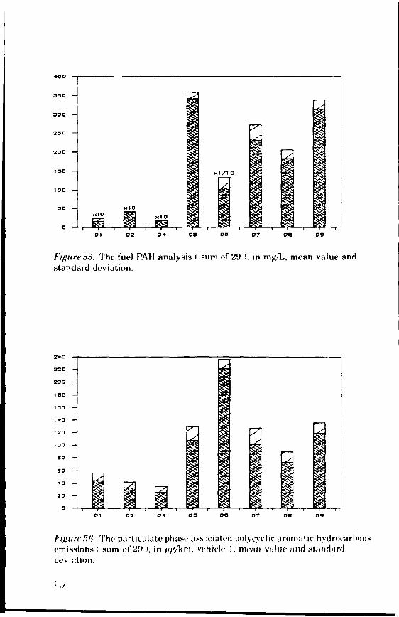
130 - X1/1O

1O0 -

3D -

Figure 55. The fuel PAH analysis ( sum of 29 ), in mg/L, mean value andstandard deviation.

Figure 56. The participate phase associated poiycyclic aromatic hydrocarbonsemissions ( sum of 29 >, in /xtf/km, vehicle 1, mean value and standarddeviation.

sno

200

2*0

200

I BO

100

Figure 57. The semi-volatile phase associated polycyclic aromatic hydro-carbons emissions (sum of 29), in /ig/km, vehicle 1, mean value and standarddeviation.

,7

.0

,3

,<•

.3

.2

.1

1

0.9

O.B

O.7

O.B

O.3

0.+

0.3

I

Figure58. The particular- phase associated 1-nitropyrcnc emissions, inkm, vehicle 1, mean value and standard deviation.

D» 03

Figure 59. " n participate phase associated polycyclic aromatic hydro-carbons < , sions (sum of 29), in /*g/km, vehicle 2, mean value and standarddeviate

Figure 60. The semi-volatile phase associated polycyclic aromatic hydrocar-bons emissions ( sum of 29 ), in //g/km, vehicle 2, mean value and standarddeviation.

• • -

13 -

1 1 -

10 -

7 -

0 -

3 -

3 -

2 -

1 -

Figure 61. The particulate phase associated 1-nitropyrene emissions, in/xg/km, vehicle 2, mean value and standard deviation.

5.6 CARBON DIOXIDE EMISSIONS AND FUELCONSUMPTION

Kerstin GräggEnvironmental SectionSwedish Motor Vehicle Inspection CompanyBox 508, S-162 15 VÄLLINGBY, SWEDEN

5.6.1 IntroductionThe emission of carbon dioxide has until recently been considered asharmless. However, since the green house effect, caused partly bycarbon dioxide, is now well known and frequently discussed there is agrowing concern about the emission of carbon dioxide from motor vehi-cles. As long as the fuel consists of fossil hydrocarbons, the contributionof motor vehicle emission to the green house effect is not avoidable.Since the diesel engine is more fuel efficient than the Otto enginefueled with gasoline (or some other fossil fuel), the diesel engine has anadvantage when the green house effect is considered.

5.6.2 Results and DiscussionsCarbon dioxide emissions were investigated in both the bus cycle andthe U.S. transient cycle. The levels of carbon dioxide emission from thetwo vehicles tested was displayed in figure 62 to 65. Carbon dioxideemissions were measured using a NDIR instrument made by Beckman(Beckman INC, USA). Fuel consumption was measured gravimetrical-ly (Mettler balance) and is displayed in figures 66 to 71. The carbondioxide emission level depends on the fuel consumption as expected.The fuel dependent carbon dioxide emission varies less than 10 r/r forvehicle 1 and seems not to depend on the driving condition tested.Corresponding values for vehicle 2 is less than 3 7r, for the bus cycle,and less than 14 cfc, for the U.S. transient cycle.

5.6.3 ConclusionsCarbon dioxide emissions and fuel consumption show a covariance.

94

13

t.a -

t.i -

i -

o.* -

o.a -

0.7 -

o.e -

os -

0.4 -

O.3 -

o.a -

o.t -

oD i D2 0 4 0 0 0 7 D»

Figure 62. Carbon dioxide emissions, in kg/km vehicle 1, mean value andstandard deviation, bus cycle.

o » -

O.B -

0.7 -

0.Ö -

0.5 -

0.4 -

0.3 -

02 -

0.1 -

Dtf"—r

04 0 5 0 7 0 6 0 »

Figure 6,1. Carbon dioxide emissions, in kg/km vehicle 1, mean value andstandard deviation, US transient cycle.

12

I.I -

t -

O.» -

o.a -0.7 -

o.e -

os -

0.4 -

O.3 -

o.a -

o.i -

o0 1 os 0 9

Figure 64. Carbon dioxide emissions, in kg/km vehicle 2, mean value andstandard deviation, bus cycle.

i

0.9 -

o.a -

0 7 -

o.e -

o.s -

O.4 -

03 -

0 2 -

O.I -

0OS 0 7

Figure HH. Carbon dioxide emissions, in k^/km vehicle 2. mean value andstandard deviation, US transient cycle.

-too -

350 -

3OO -

2SO -

2O0 -

ISO -

IOO -

SO -

O1 02 OS 07

Figure 66. Fuel consumption, in g/km vehicle 1, mean value and standarddeviation, bus cycle.

3O0aso -aeo -2*0 -

220 -

200

160 -

IOC -

M

t:

i „ J

\I0 1 0 2 OS 06 0 7 OS 09

' ii>urv67. Fuel consumption, in g/km vehicle 1, mean value and standardt viation, US transient cycle

t«0

ISO

140

130

120

ttO

too»oao70oo5040302010o

01 02 OS 07 D9

Figure 68. Fuel consumption, in g/Hph, vehicle 1, mean value and standarddeviation, ECE R49 cycle.

400

350 -

300 -

250 -

200 -

150 -

100 -

50 -

D1 D2 0 7 OS 0 9

Figure 69. Fuel consumption, in #/km vehicle 2, mean value and standarddeviation, hus cycle.

zooaao28O

24O

220

200

160

I4O120100BO

«o40

20

oD2 D4 OS 0 7 09

Figure 70. Fuel consumption, in g/km vehicle 2, mean value and .standarddeviation, US transient cycle.

170180 -

ISO -140 -130 -

12O -

110 -100 -

90 -

so -70 -

so -50 -40 -30 -SO -10 -0

01 02 04 05 06 07 08 09

Fifjurc 71. Fuel consumption, in g/Hph vehicle 2, mean value and standarddeviation, KCE R49 cycle.

6 Biological Testing

6.1 MUTAGENICITY TESTS

Ulf Rannug and Helene BramstedtDepartment of GeneticsStockholm UniversityS-106 91 STOCKHOLM, SWEDEN

6.1.1 IntroductionThe initial step in a risk assessment is the risk identification, which forhealth effects, such as cancer, or other effects related to genotoxicity ispreferentially carried out by means of short-term tests. Especially forcomplex environmental mixtures, the Ames mutagenicity tests inSalmonella typhimurium has shown to be a useful tool. In our previousstudies on automobile exhausts, the Ames test has played an importantrole in the characterization of both the particulate part and the semi-volatile part of the exhaust emission (Rannug and Sundvall, 1985;Alsberg et al., 1985). Also, in the characterization of exhaust emissionsfrom vehicles run on different types of fuel, comparisons based onmutagenicity tests using Salmonella typhimurium have been useful(Rannug 1983; Rannug and Sundvall, 1985).

Several of the unregulated pollutants present in the exhaust emissionmay originate from components in the fuel. It is, therefore, possiblethat a reduction of the amount of mutagens and carcinogens in theemission and, thereby, a reduction in the health impact from automo-bile exhaust emissions could be achieved by modifying the fuel-Recently, the effect of fuel PAC on the emissions of PAC and the muta-genicity of the emissions was studied (Westerholm et al. 1988). Fromthis study we concluded that the lowest mutagenic effect of the partic-ulate extracts of the exhausts was seen with a fuel containing onlymonocyclic aromatics, while the highest mutagenicity was seen with afuel containing a full range reformat, implying that a full reformatcontains more mutagens and/or produces during combustion. Theseresults indicated that a more detailed study using several diesel fuelswith different properties, e.g. different content of aromatics, would giveimportant information on the relationship between chemical propertiesof the fuel and genotoxic properties of the emissions. The presentinvestigation was carried out to elucidate the.se relationships.

I (K)

6.1.2 Materials and MethodsThe mutagenicity tests were carried out as described by Maron andAmes (1983). with Salmonella typhimurium strains TA98 and TA100.The plate incorporation-assay was basically followed, though histidine(0.1 umol/plate) and biotin (0.1 umol/plate) were added to the minimalmedium instead of to the soft agar as in our previous tests on exhaustemission samples. The samples were tested with and without the addi-tion of the liver S-9 fraction from Aroclor-pretreated male Sprague-Dawley rats. The amount of the 10*X S9-mix per plate was 0.5 mi, ie. 50fx\ S9 fraction/plate. All samples (three per fuel and vehicle), dissolvedin dimethyl sulfoxide (MERCK), were tested at three different concen-trations each in triplicate, usually corresponding to 0.5, 1.0 and 2.0meters driving distance. Fuels D4, D5 and D6 showed, with one of thevehicles, a much higher mutagenicity and to avoid toxicity these sam-ples were tested at lower concentrations corresponding to 0.25, 0.5 and1.0 meters. Each experiment included positive controls for checking theactivity of the S9 and the mutability of the tester strains using benzo(a)pyrene and quercetin at the amount of 2.5 fig and 100 ^g per plate,respectively. For quercetin the mutagenicity was approx. 870 revert-ants on strain TA98 and approx. 650 revertants per plate on strainTA100. B(a)P showed a mutagenic activity of about 230 revertants perplate on strain TA98 and about 890 revertants per plate on strainTA100. These results are in accordance with earlier data. The muta-genic potency of each sample was determined by linear regressionanalysis and given as revertants per kilometer driving distance. Thedata given in the figures are the mean value from the three samplesfrom each fuei and vehicle, except for the semi-volatile phase where thevalue including standard deviation is taken from the regression analy-sis at one sample from each fuel and vehicle.

6.1.3 Results and Discussions

Particulate phaseAll results from the mutagenicity tests of the particulate phase arebased on the arithmetical mean from three tests per fuel and vehicle.

Vehicle one:

All individual emission samples except three, one of the Dl samples onTA100-S9 and one of the D8 samples on TA98+S9 and TA100-S9,resulted in significant mutagenic effects on both tester strains (Fig. 72

101

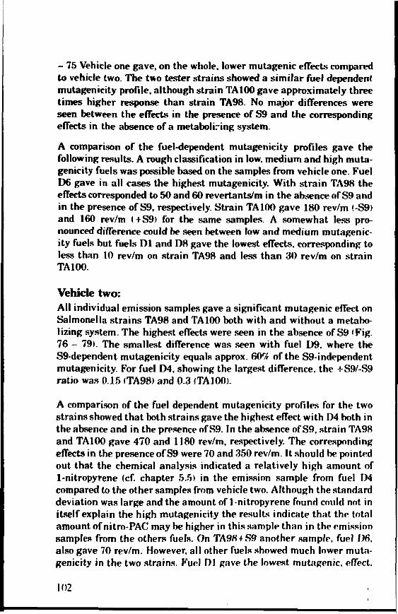
- 75 Vehicle one gave, on the whole, lower mutagenic effects comparedto vehicle two. The two tester strains showed a similar fuel dependentmutagenicity profile, although strain TA100 gave approximately threetimes higher response than strain TA98. No major differences wereseen between the effects in the presence of S9 and the correspondingeffects in the absence of a metaboliring system.

A comparison of the fuel-dependent mutagenicity profiles gave thefollowing results. A rough classification in low, medium and high muta-genicity fuels was possible based on the samples from vehicle one. FuelD6 gave in all cases the highest mutagenicity. With strain TA98 theeffects corresponded to 50 and 60 revertants/m in the absence of S9 andin the presence of S9, respectively. Strain TA100 gave 180 rev/m (-S9)and 160 rev/m (+S9) for the same samples. A somewhat less pro-nounced difference could be seen between low and medium mutagenic-ity fuels but fuels Dl and D8 gave the lowest effects, corresponding toless than 10 rev/m on strain TA98 and less than 30 rev/m on strainTA100.

Vehicle two:All individual emission samples gave a significant mutagenic effect onSalmonella strains TA98 and TA100 both with and without a metabo-lizing system. The highest effects were seen in the absence of S9 <Fig.76 - 79». The smallest difference was seen with fuel D9, where theS9-dependent mutagenicity equals approx. 60% of the S9-independentmutagenicity. For fuel D4, showing the largest difference, the +S9/-S9ratio was 0.15 (TA98) and 0.3 ITAIOO).

A comparison of the fuel dependent mutagenicity profiles for the twostrains showed that both strains gave the highest effect with D4 both inthe absence and in the presence of S9. In the absence of S9, strain TA98and TA100 gave 470 and 1180 rev/m, respectively. The correspondingeffects in the presence of S9 were 70 and 350 rev/m. It should be pointedout that the chemical analysis indicated a relatively high amount of1-nitropyrene (cf. chapter 5.5) in the emission sample from fuel D4compared to the other samples from vehicle two. Although the standarddeviation was large and the amount of 1-nitropyrene found could not initself explain the high mutagenicity the results indicate that the totalamount of nitro-PAC may be higher in this sample than in thp emissionsamples from the others fuels. On TA98+S9 another sample, furl 1)6,also gave 70 rev/m. However, all other fuels showed much lower muta-genicity in the two strains. Fuel Dl gave the lowest mutagenic, effect,

102

giving 10 and 80 rev/m in the presence of S9 on TA98 and TA100,respectively. Other fuels, belonging to the low mutagenicity class, wereD7 and D8 when tested on TA98+S9 or TA98-S9. For strain TAiOO thesame fuels gave the lowest effects, and in the presence of S9, D9 alsobelongs to this class. Apart from D4, fuel D6 also gave a high muta-genie effect in the presence of S9. This was also true for fuel D5 onTA100+S9- The rest of the fuels resulted in emissions with mediumeffects. In conclusion, all strains indicated that fuel D4 generates highmutagenicity emissions while the low mutagenicity fuels were Dl, D7and D8. The fuels can therefore be classified on the basis of muta-genicity of their emissions in high, low or medium genotoxic fuels.

Blank samples:Blank filters from the dilution tunnel were also tested for mutagenicityon both tester strains. Some of the samples gave a significant muta-genic effect which would equal no more than 6 rev/m in strain TA98and approx. 20 rev/m in TA100. However, there was no consistency inthe mutagenicity and these low effects did not change the rank orderbetween the different fuels. The only fuel that gave a low effect, in thesame range as the blank samples was fuel Dl.

Semi-volatile phaseThe results from the mutagenicity tests of the semi-volatile phase arebased on one sample per fuel and vehicle. The semi-volatile phase wascollected with absorbent technique, polyurethane foam (PUF) accord-ing to Westerholm et al. 11991).

Vehicle one:Again lower mutagenicity was seen with samples from vehicle onecompared to the samples from vehicle two and, therefore, several sam-ples did not show statistically significant effects. The PUF techniqueindicated that Dl was not mutagenic in either of the strains while D4was the most mutagenic sample in the absence of S9 and the secondmost mutagenic sample with metabolism. All the mutagenic samplesgave between 20 and 40 rev/m in TA100+S9.

The mutagenic profile of the semi-volatile phase from this vehicle didnot show the typical mutagenicity pattern on TA100 with and withoutS9 as mentioned below. With this vehicle, the rnutagenicity in thepresence of S9 was either similar to or higher than the mutagenicity inthe absence of S9.

103

Vehicle two:AH but one sample from the vehicle , sample 0 6 on TA98-S9, gavesignificant mutagenic effects in both tester strains with and without ametabolizing system.

The fuel dependent mutagenicity profile from the PUF samples in bothtester strains gave the following results. Fuel D4 gave the highesteffects in both strains in the absence of S9, while the lowest effects wereseen with D6 and D9. In the presence of the metabolizing system, thefuel-dependent pattern was different. The highest mutagenic effectswere seen with D6. 540 rev/m on TA98 and 190 rev/m on TA100,respectively, followed by D5 (TA98+S9 gave 50 rev/m) or D4(TA100+S9 gave 150 rev/m). A comparison of the two strains in theabsence of S9 showed that the mutagenic response was higher in TA100in accordance with our earlier data < Westerholm et al. 1986). AH sam-ples, except D9 which gave a similar effect with and without S9 onstrain TA100, showed a higher effect on TA100 in the absence of ametabolizing system. This is also in accordance with earlier data ondiesel exhaust emissions (Westerholm et al. I986)-

Blank samples:The blank samples for the semi-volatile phase showed little consistencyalso and especially some of the mutagenic emission samples from vehi-cle one gave effect of the same magnitude as some of the blank sampleswhich indicate that small differences between fuels in this connectionmay be random and not truly reflect a fuel difference.

6.1.4 ConclusionsThe mutagonicity profiles of the emission samples were both fuel andvehicle dependent. Roughly, however, the fuels could be classified as alow, medium or high mutagenicity fuel based on the mutagenicity inSalmonella typhimurium (Ames test) of the generated emissions.

Vehicle no. 1: The high level fuel was F)6 (particles) and, in the case ofsemi-volatile phase, fuel 1)4. I ow level fuels were fuel 1)1, all cate-gories, and 1)8 (all participate samples).

Vehicle no 2: High level fuel was 1)4 (all particulate phases and alsosemi-volatile phases in the absence of a metabolizing system), l owmutagenicity fuel was 1)1 (all categories) together with 1)7 and 1)8(particles) and 1)9 (semi-volatile phase).

KM

The statistical analyses see Appendix A:2, showed a good correlationbetween fuel variables and biological effects ir = 0.9, Fig. 113) as wellas between chemical emission and biological effects (r = 0.92, Fig. 117).The most important fuel variables for the correlation to the biologicaleffects seem to be distillation interval for 90% and FBP while energycontent was negatively correlated. The other most important variableswere the content of fuel PAC.

The most important biological effects for the correlation to the fuelvariables were the mutagenicities of the particulate phase on bothSalmonella tester strains (Fig. 112).

The biological effects also showed a strong correlation to the chemicalemission variables (r = 0.92). The most important variables were theemissions of PAC, especially the sum of PAC and the individual PACfluoranthene and 2-methylpyrene in the particulate phase and sum ofPAC and pyrene in the semi-volatile phase (Fig. 115). It should also benoted that the contribution of benzo(a)pyrene to the correlation wasnegative and of less importance than the PAC mentioned above.

Finally, the model showed excellent correlation between observed andpredicted values for the biological variables, e.g., mutagenicity of thesemi-volatile phase on TA98-S9 (r = 0.98, Fig. 118).

6.1.5 ReferencesAJsbergT.,Stenberg U., Westerholm R, StrandelJ M , Rannutf U . eta). (1985).Chemical and Biological Characterization of Organic Material from GasolineExhaust Particles. Envir. Sci. Tech. 19, 43-50.

Maron D. M. and Ames B. N.(1983). Revised Methods Tor the SalmonellaMutagenicity Test. Mut. Res. 113, 173-215

Rannug U. (19&3). Data from Short-term Tests on Motor Vehicle Exhausts.Environm. Health Persp. 47, 161-169

Rannug U. and Sundvall A. (1985). Mutagcnic Properties of Gasoline Ex-hausts. Environm. Intern. 11, 303-309.

Wcstcrholm R., AlshcrgT, Frommclin Å., Strandcll M., Rannug II., WinquistL., Grigoriadis V, and Egchack K-E (1988). Effect of Fuel Poiycyclic AromaticHydrocarhon Content on the Emission of Polycyclic Aromatic Hydrocarbonsand other Mutagenic Substances from a Gasoline-fueled Automobile. Envi-ronm. Sci. Tech. 22, 925 930

105

Westerholm R . A Isberg T. Strandell M . Frommelin A.. Grigoriadis V. Hantzaridou A . Maitra G . Winquist L . Rannug U . Egeback K-E and BertilssonT.II986». Chemical Analysis and Biological Testing of Emissions from aHeavy-duty Diesel Truck With and Without Two Different Particulate Traps.SAE-Paper 860014.

Westerholm R . Almen J . Hang L , Rannug U . Egebäck K-E. and Grägg K.11991) Chemical and Biological Characterization of Particulate. Semi-Volatileand Gas Phase Associated Compounds in Diluted Heavy Duty Diesel Ex-hausts: A Comparison of Three Different Semi-volatile Phase Samplers. Envi-ronm. Sci. Tech. Vol. 25, 332-338.

DO

Figure 72. Mutagenicity, particulate phase, TA98-S9, in revertants/m,vehicle 1, mean value and standard deviation, bus cycle.

Figure 73. Mutagenicity, particulate phase, TA98+S9, in revertants/m,vehicle 1, mean value and standard deviation, bus cycle.

107

22O

2OO -

1BO -

too -

12O -

1OO -

BO —

OO -

•O -

3O —

O

Figure 74. Mutagenicity, particulate phase, TA100-S9, in revertants/m,vehicle 1, mean value and standard deviation, bus cycle.

2 0 0

Figure 75. Mutagenicity, particulate phase, TAJ00+S9, in revertants/m,vehicle 1, mean value and standard deviation, bus cycle.

108

Figure 76. Mutagenicity, particulate phase, TA98-S9, in revertants/m,vehicle 2, mean value and standard deviation, bus cycle.

130

12O -

110 -

100 -

9O -

• O -

70 -

00 -

SO -

•O -

30 -

SO -

10 -

O

oe

Figure 77. Mutagenicity, particulate phase, TA98+S9, in revertants/m,vehicle 2, mean value and standard deviation, bus cycle.

I Of)

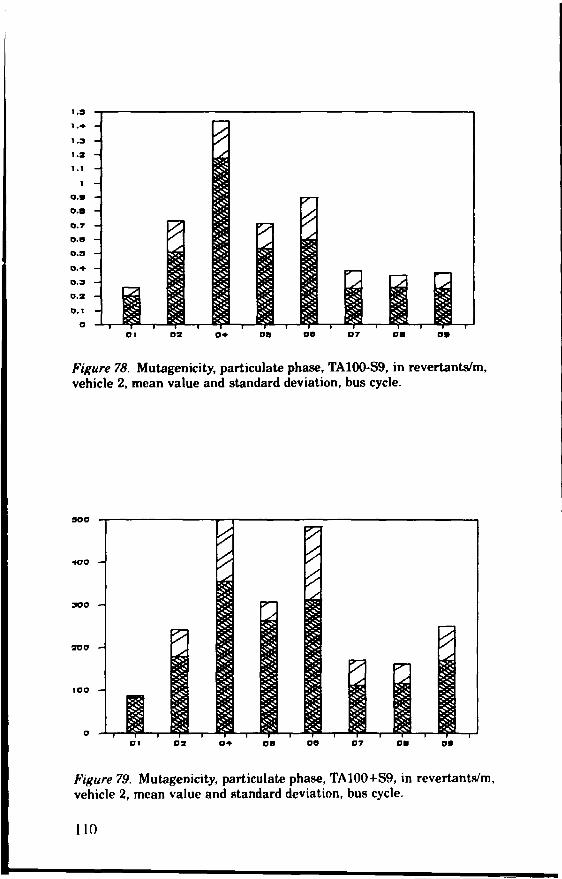
1.3

1 . *

1.3

1.2

1.1

1

O.»o.aO.TO.B0.3

o . * -

0.3 -

0.3 -

0.1 -

O

Figure 78. Mutagenicity, particulate phase, TA100-S9, in revertants/m,vehicle 2, mean value and standard deviation, bus cycle.

200 -

01 02 O+ OB 00 07 DM 0 *

Figure 79. Mutagenicity, particulate phase, TA100+S9, in revertants/m,vehicle 2, mean value and standard deviation, bus cycle.

110

11 -

IO -

3

1

O

-1

-a-3

Figure 80. Mutagenicity, semi-volatile phase, TA98-S9, in revertants/m,vehicle 1, mean value and standard deviation, bus cycle. NS = Not Significant.

•o

no -

7O -

00 -

so -

•o -

3O -

2O -

1 O -

O

-1 O

Figure HI. Mutagenicity, semi-volatile phase, TA98+S9, in revortants/m,vehicle 1, mean value and standard deviation, bus cycle. NS = Not Significant.

II

to -

•o -

33 -

3O -

23 -

ZO -

13 -

1O -

3 -

O -

— 3 -

-1O -O2 O* D3 DO O7 Oti 09

Figure 82. Mutagenicity, semi-volatile phase, TA100-S9, in revertants/m,vehicle 1, mean value and standard deviation, bus cycle. NS = Not Significant.

33 -

30 -

as -

2O -

13 -

)0 -

s -

oOB

Figure 83. Mutagenicity, semi-volatile phase, TA100+S9, in revertants/m,vehicle 1, mean value and standard deviation, bus cycle. NS = Not Significant.

12

Figure 84. Mutagenicity, semi-volatile phase, TA98-S9, in revertants/m,vehicle 2, mean value and standard deviation, bus cycle. NS = Not Significant.

120

no -IOO -

90 -

BO -

7O -

DO -

SO -

*0 -

3O -

2O -

10 -

O

i/a

03

Figure 85. Mutagenicity, semi-volatile phase, TA98+S9, in revertants/m,vehicle 2, mean value and standard deviation, bus cycle.

13

3*O32O

azo200

)3O -100 -

ao -00 -•o -20 -o

Figure 86. Mutagenicity, semi-volatile phase, TA100-S9, in revertants/m,vehicle 2, mean value and standard deviation, bus cycle.

21 O2OOISOISO170ISO130

190120

no1OO90ao70easo•oao2010o OS

Figure 87. Mutagenicity, semi-volatile phase, TA100+S9, in revertants/m,vehicle 2, mean value and standard deviation, bus cycle.

114

DIOXIN RECEPTOR AFFINITY TESTS

Grant Mason, Annemarie Witte and Jan-Åke GustafssonDepartment of Medical Nutrition, Karolinska InstituteHuddinge Hospital F60, NovumS-141 86 HUDDINGE, SWEDEN

6J2.1 IntroductionBound to particles found in urban air is a highly complex mixture oforganic compounds. Many of these environmental contaminants areproduced during the incomplete combustion of organic matter from forexample municipal incinerators, the burning of fossil fuels and frommotor vehicle exhausts. The biological and adverse health effects ofthese compounds are only partly known. In mammalian tissues, metab-olic activation of compounds to more chemically reactive species is akey step in the sequence of events leading to genotoxicity and carcino-genicity. With regard to poiycyclic aromatic hydrocarbons (PAH), vari-ous cytochrome P450 isozymes preferentially catalyze this activation.In the rat, two of these isozymes, P450c and P450d (IA1 and IA2;Nebert et al. 1987), are known generally as aryl hydrocarbon hydroxy-lase (AHH) (Conney, 1982).

Studies in this laboratory have shown that extracts of particulatematter from urban air and automobile exhausts contain compoundswith high affinity for the receptor protein in rat liver which specificallybinds 2,3,7,8-tetrachlorodibenzo-p-dioxin (TCDD) (Toftgård et al.1983,1985; Alsberg et al. 1985). Affinity for this receptor has beenshown to correlate with the ability to induce AHH activity both in vivoand in vitro (Poland and Knutson, 1982; Mason et al. 1985, 1986; Safe,1986). Indeed, further studies from this laboratory have shown thatAHH activity can he induced in the H4IIE cell line by such particulateextracts and that such induction correlates well with receptor affinity(Franzénetal 1988).

AHH induction may be of importance in an individual's susceptibilityto cancer. Thus, mouse strains which display a high AHH inducibilitysuffer from a higher incidence of lung tumours in response to 3-methyl-cholanthrene than strains with low AHH inducibility (Kouri et al.1980). Induction of AHH has been shown to occur in the liver and lungsof research animals after cigarette smoke inhalation (Abrahamsson

115

and Hutton, 1975). It has also been reported that diesel exhaust gaseswill cause AHH induction in test animals (Greenlee and Poland, 1979).Furthermore, it has been shown that AHH activity increases in thelungs of mice placed in heavily industrialised areas of the USA (Mos-tardi et al. 1981). It is assumed that it is the PAH components ofcigarette smoke and diesel exhaust that are responsible for the observ-ed induction of AHH.

Induction of AHH, per se, may therefore play a role in the mechanismof toxicity and carcinogenicity of the non-halogenated PAH, which areextensively metabolised by this mono oxygenate system, to chemicallyreactive species capable of binding to cellular macromolecules (e.g., theformation of benzo(a)pyrene-7,8-diol-9,10-epoxide from benzoia)py-rene). Furthermore, receptor binding has been shown to be of impor-tance in the initiation of a variety of other biological and toxic effects ofthe halogenated and non-halogenated PAH including, for example,embryotoxicity, cellular hyperplasia and differentiation, tumour pro-motion and depletion of lymphoid tissue (reviewed in Poland and Knut-son, 1982).

Thus, the determination of a compound's TCDD receptor binding affin-ity and its ability to induce AHH provides a measure of its potential foreliciting the toxic effects associated with this group of compounds.

6.2.2 Materials and MethodsMaterialsHydroxylapatite (Bio-Gel HTP) was obtained from Bio-Rad (Rich-mond.CA). 2,3,7,8-tetrachloro-l,6, f'HI dibenzo-p-dioxin (spec. act. 40Ci/mmol)(| :)H|TCDD) and 2,3,7,8-tetrachlorodibenzofuran (TCDF) wereobtained from Chemsyn Science Laboratories (Lenexa, KS). All otherchemicals were of analytical grade from either Sigma Chemical Com-pany (St. Louis, MO) or Merck A.G. (Darmstadt, F.R.G.)

Preparation ofcytosolSix-week old male Sprague-Dawley rats were sacrificed by cervicaldislocation and their livers immediately per fused in situ with ice-coldEPGM buffer (1 mM EDTA, 20 mM potassium phosphate, 107r w/vglycerol and 2 mM B-mercaptoethanol). The livers were then rapidlyexcised and homogenised in EPGM buffer. The homogenate was cen-trifuged at 75,000 x g for 105 min and the resulting clear supernatantwas used as cytosol. Cytosol was stored in aliquots at -80 C untilneeded.

116

Preparation of samplesThe vehicle exhaust extracts were received from the Department ofAnalytical Chemistry, Stockholm University, dissolved in acetone (seesection 5.5). Prior to assay in our laboratory, the acetone was evaporat-ed off under nitrogen and the samples redissolved in dimethyl sulph-oxide (DMSO). Further dilutions from this stock were also made inDMSO.

Measurement ofdioxin receptor-binding affinityThe dioxin receptor-binding affinities of samples were measured usingan hydroxylapatite (HAP) assay developed in our laboratory (Poell-inger et al. 1985). This assay, based on the sequential washing ofHAP-immobilized receptor with phosphate buffers of increasing ionicstrength, was developed to provide a rapid and accurate receptor assay.To determine the binding affinities of samples, competition experi-ments are carried out with increasing concentrations of sample againsta standard concentration of radio-labelled TCDD. The relative bindingaffinities of the samples are then expressed indirectly as EC^, valuescalculated from log-logit plots of the competition for [ 'HlTCDD-bind-ing. ECW values are the concentrations of competitors that are requiredto reduce the binding of [3H]TCDD to its receptor by 50%.

All procedures were carried out at 4°C. Cytosol was thawed on ice anddiluted to 2 mg/ml with EPGM buffer. One ml aliquots of cytosol werepipetted into siliconized glass tubes. To sets of 5 tubes were addedvarying concentrations of sample in 5 fih aliquots of DMSO. In eachassay 5 /xL of DMSO alone were added to one tube to act as a blanksample. To a further tube were added 5 fib of TCDF in DMSO to a finalconcentration of 200 nM to act as a positive control. To all the tubesf'HjTCDD in 5 /xL of DMSO to a final concentration of 1 nM was thenadded. After mixing, the tubes were incubated for 16 hr at 4°C. Aliqu-ots (0.4 ml) of incubates were then pipetted in duplicate into Eppeiidorftubes and 0.4 ml of a 1:1 suspension of HAP in EPGM added. Thesamples were left to incubate for 15 min, with vortexing every 5 min.Meanwhile, duplicate 50 fxh aliquots of the original incubates weretaken for liquid scintillation counting to determine total added radio-activity and to check that the solubility limits of the [3HJTCDD werenot exceeded. The samples were now centrifuged at maximum speed inan Eppendorf 5413 centrifuge for 5 min. The supernatant was thenremoved from the pelleted material by aspiration. 0.4 ml of 75mM

117

phosphate buffer was then added and the tube vortexed and allowed tostand for 5 min. The HAP was then repelleted and the previous wash-ing step repeated. The receptor-ligand complexes were then extractedby two washes with 0.4 ml of 175 mM phosphate buffer. These washeswere removed from the pelleted HAP by pipette and transfered toscintillation vials. Four ml of liquid scintillant was added and theamount of [3H|TCDD present determined. Specific binding was deter-mined as the difference in the level of protein-bound ligand in theabsence or presence of the 200-fold molar excess of unlabeled compet-itor (TCDF). The specific binding of [3H1TCDD in the presence of ex-haust samples was expressed as a percentage of the specific binding inthe control incubation (PHITCDD + DMSO). The EC,,, value for theindividual exhaust samples was calculated from log-logit plots of thecompetition for ['HITCDD-binding where logit b = In (b/l-b). The log-logit plots were calculated using linear regression analysis. Three sep-arate emissions samples were run for each fuel (see section 5.5) in orderto determine the ECW values of the particulate phase emissions. TheECW of each sample was determined at least twice. ECW values givenare the mean +/- standard deviation of the three samples for each fuel.For the semi-volatile phase determinations only one pooled sample wasavailable for each fuel (see section 5.5). ECW values for these sampleswere determined at least twice, usually three times. ECW values givenare the mean +/- standard deviation of these determinations. Statisti-cal analysis was performed by analysis of variation and the Student-Newman Keuls test.

6.2.3 Results and DiscussionsFor each fuel sample, extracts of both the particulate and the semi-volatile phase (collected using the PUF technique-see section 5.5) asso-ciated emission products were tested for TCDD receptor binding activ-ity. The binding affinities were expressed as ECr>0 values (see above)and are shown in figures.

Particulate phaseVehicle one:The EC50 values for binding to the dioxin receptor of the particulatephase exhaust emissions from vehicle one are shown in figure 88.Dioxin receptor binding activity was observed in all the emission sam-ples tested. The EC , values for binding to the dioxin receptor of thesamples varied over an approximately 8-fold range. The mean ECr,ncalculated for fuel D7 is not significantly different from that of any

118

other fuel due to the large variation. Insufficient sample amount pro-hibits further estimations of this sample's ECM and it has been exclud-ed from the following comparisons. Fuel Dl displayed the lowest bind-ing affinity with the highest <p<0.01) ECW of 0.24 m/ml. Fuel D6produced the emission sample with the highest affinity for the dioxinreceptor with the lowest EC^ value of 0.04 m/ml. This EC^ was signif-icantly lower than those for fuels D1,D2,D5 <P<0.01) and D8 (p<0.05)but not significantly different from those of the remaining fuels.

Vehicle two:Figure 89 shows the ECW values for dioxin receptor binding of theparticulate phase exhaust emissions from vehicle two. Dioxin receptorbinding activity was again observed in all the samples. Due to technicaldifficulties an EC , value for fuel D4 could not be estimated and in-sufficient sample remained to repeat the analysis. On examination ofthe fuel dependency of the ECW values obtained, it was observed thatalthough fuel D6 once again produced the emission with the highestreceptor binding affinity with an ECW of 0.04 m/ml. there were, Howev-er, no significant differences between any of the fuels with regard toemission receptor ECWS of their emissions. Only a 2-fold variation inECW values was observed in the samples from vehicle two.

The EC;,, values for dioxin receptor binding of particulate associatedemission products in this study compare favorably with those deter-mined in previous studies of both diesel- and gasoline-fuelled vehicleemissions. Ålsberg et al. (1985) reported an EC^ of 0.04 m/ml for theparticulate associated emissions from a gasoline-fuelled automobile.However, EC^ as low as 0.005 and 0.002 m/ml., respectively, have beendetermined for exhaust particulate extracts from gasoline- and diesel-driven automobiles (Toftgård, personal communication).

From the data derived from vehicle one, where there was a greaterspread in the binding affinities, it was observed that there was acorrelation (see later multivariate analysis results) between the affin-ity of an exhaust sample for the dioxin receptor and the PAH content ofthe sample and of the original fuel sample. That is to say that fuels withhigh PAH content gave rise to particulate emissions with high PAHcontents and high dioxin receptor binding activities and vice versa;fuels with low PAH content gave rise to emissions with lower PAHcontents and lower dioxin receptor binding activities. This observationis not surprising as it is generally believed that it is compounds of the

119

PAH-type which are responsible for the binding activities seen. How-ever, it is not, as yet, certain which compounds are responsible for thedioxin receptor binding activity elicited by vehicle exhaust particulateextracts. It is probably not due to dibenzo-p-dioxins or related com-pounds as the levels of these compounds are too low to produce theobserved receptor binding activities (Toftgård et al. 1985). The identityof which compounds are responsible for the observed dioxin receptorbinding is currently under investigation.

Semi-volatile phaseVehicle one:The ECJO values for binding to the dioxin receptor of the semi-volatilephase exhaust emissions from vehicle one are shown in figure 90.Dioxin receptor binding activities were observed in all the samplesexcept that from fuel D7 (EC^ > 0.5 m/ml limit of detection at thesample dilutions used in the assay). Fuel 0 6 gave rise to the semi-volatile phase emission with the highest affinity for the dioxin receptorwith the lowest ECW of 0.02 m/ml. With the exception of the samplefrom fuel Dl, the dioxin receptor binding activities of the semi-volatilephase emissions were similar or lower than those of the correspondingparticulate phase emissions.

Vehicle two:Figure 91 shows the EC;*, values for dioxin receptor binding of thesemi-volatile phase exhaust emissions from vehicle two. No result wasobtained, due to technical difficulties, for three of the fuels (D5,D6 andD7). However, sufficient sample remains to re-determine these ECW

values (see below), unfortunately not before preparation of this report-No detectable dioxin receptor binding activity was seen in the samplesarising from fuels Dl, D4 and D8. Receptor binding activity was seen inthe semi-volatile phase emissions from fuels D2 and D9 with EC^ of0.04 and 0.02 m/ml respectively.

This is the first study to demonstrate the presence of compounds withaffinity for the dioxin receptor in the semi-volatile phase of dieselexhaust emissions. This was a .surprising result as it was expected thatcompounds emitted in this phase would be of lower molecular weightand size than would be expected of good ligands to the dioxin receptor. Ithas been shown that, characteristically, good ligands for the dioxinreceptor are planar molecular which, when their atomic van der Waals

120

radii are included, fit into a rectangle of 6.8 x 13.7 Å (Gillner et al.1985). Such compounds might be expected to have a low volatility andthus appear to a much greater degree in the particulate phase. Indeed,the larger PAHs were found to a greater extent in the particulatephase, whereas the smaller 2 and 3 ringed PAHs were mainly in thesemi-volatile phase. It has been suggested, based on mathematicalmodelling of particle/vapor partitioning, that possibly 20-60% ofTCDD in ambient air would exist in the vapor phase (Bidleman, 1988).Indeed, it has been reported that tetra- and pentachlorinated dioxinsand dibenzofurans pass through glass fibre filters during urban airsampling (Eitzer and Hites, 1986). It will be of immense interest toidentify those compounds present in the semi-volatile phase with affin-ity for the dioxin receptor.

The large variation in some of the EC50 values and the non-determina-tion of others for the semi-volatile phase samples prevents any conclu-sions being drawn as to what factors determine the activities observed.However, sufficient amounts of every semi-volatile phase sample re-mains for us to repeat our determinations of their EC^. These experi-ments are now underway.

6.2.4 ConclusionsIn conclusion, substantial amounts of dioxin receptor binding activityare present in both the particulate and semi-volatile phase of dieselexhaust emissions. It will be of great interest to identify which com-pounds present in the emissions are responsible for this activity. Worktowards this is currently in progress in our laboratory. The aboveresults also, importantly, indicate that it may be possible to design fuelswith reduced dioxin receptor binding activity associated with theirexhaust emissions.

6.2.5 ReferencesAbrahamsson R. and Hutton J. (1975) Effects of Cigarette Smoking on ArylHydrocarbon Hydroxylase Activity in Lungs and Tissues of Inbred Mice.Cancer Res. Vol. 35, pp 23-29.

Alsberg T., Stenberg U., Westerholm R., Strandell M., Rannug U., Sundvall A.,Romert L., Berson V., Pettersson B., Toftgård R., Franzén B., Jansson M.,Gustafsson J.-Å. Egebäck K-E. and Tejle G. (1985) Chemical and BiologicalCharacterization of Organic Material from Gasoline Exhaust Particles. Envi-ron. Sci. Technol. Vol. 19, 43-50.

121

Bidleman T. (1988) Atomospheric Processes. Environ. Sci. Technol. Vol. 22,361-387.

Conney A. (1982) Induction of Microsomal Enzymes by Foreign Chemicals andCarcinogenesis by Polyaromatic Hydrocarbons. Cancer Res. Vol. 42,4875-4917.

Eitzer B. D. and Hites R. A. (1986) Int. J. Environ Anal. Chem. 27, 215-230.

Franzén B., Haaparanta T., Gustafsson J.-Å. and Toftgård R. (1988) TCDDReceptor Ligands Present in Extracts of Urban air Particulate Matter LnduceAryl Hydrocarbon Hydroxylase Activity and Cytochrome P-450c Gene Expres-sion in Rat Hepatoma Cells. Carcinogenesis, Vol 9, 111-115.

Gillner M., Bergman J., Cambillau C, Fernström B. and Gustafsson J.-Å.(1985) Interactions of Indoles with Specific Binding Sites for 2,3,7,8-tetra-chlorodibenzo-p-dioxin in Rat Liver. Mol. Pharmacol. Vol. 28, 357-363.

Greenlee W.R. and Poland A.P. (1979) Nuclear Uptake of 2,3,7,8- tetrachloro-dibenzo-p-dioxin in C57BL/6J and DBA/2J Mice: Role of the Hepatic CytosolReceptor Protein. J. Biol. Chem. Vol. 254, 9814-9821.

Kouri RE., Billups L.H., Rude T.H., Whitmore C.E., Sass B. and Henry C.J.(1980) Correlation of the Inducibiiity of Aryl Hydrocarbon Hydroxylase withSusceptibility to 3-methylcholanthrene-induced Lung Cancers. Cancer Lett.Vol. 9, 277-282.

Mason G. Sawyer T., Keys B., Bandiera S., Romkes M., Piskorska- Pliszc-zynska J., Zmudzka B. and Safe S. (1985) Polychlorinated Dibenzofurans(PCDFs): Correlation between in Vivo and in Vitro Structure-activity Rela-tionships. Toxico'. Vol. 37, 1-12.

Mason G., Farrell K., Keys B., Piskorska-PIiszczynska J., Safe L. and Safe S.(1986) Polychlorinated Dibenzo-p-dioxins: Quantitative in Vitro and in VivoStructure-activity Relationships. Toxicol. Vol. 41, 21-31.

Mostardi R.A., Ely D.L., Liebelt A., Grossman S. and Pu M.M. (1981) In-ducibiiity of Aryl Hydrocarbon Hydroxylase in BALB/c/ki Mice Exposed toUrban Air Pollution. Toxicol. Environm. Health, Vol. 7, 809-815.

Nebert D.W., Adesnick M., Coon M. J., Estabrook R.W., Gonzalez F.J., Guen-gerich FP., Gunsalus I.C., Johnson E. F, Kemper B., Levin W., Phillips I.R.,Sato R. and Waterman M.R. (1987) The P450 Gene Superfamily: Recom-mended Nomenclature. DNA Vol. 6, 1 -11.

Poellinger L., Lund J., Dahlberg E. and Gustafsson J.-Å. (1985) A Hydroxyla-patite Microassay for Receptor Binding of 2,3,7,8- tetrachlorodibenzo-p-dioxinand 3-methylcholanthrene in Various Target Tissues. Anal. Biochem. Vol. 144,371-384.

122

Poiand A. and Knutson J.C. (1982) 2,3,7,8-Tetrachlorodibenzo-p-dioxin andRelated Halogenated Aromatic Hydrocarbons: Examination of the Mechanismof Toxicity. Ann. Rev. Pharmacol. Tbxicol. Vol. 22, 517-554.

Safe S. (1986) Comparative Toxicology and Mechanism of Action of Poly-chlorinated Dibenzo-p-dioxins and Dibenzofurans. Ann. Rev. Pharmacol. Tox-icol. Vol. 26, 371-399.

Toftgård R-, Franzén B., Gustafsson J.-Å. and Löfroth G. (1985) Character-ization of TCDD-receptor Ligands Present in Extracts of Urban ParticulateMatter. Environment International, Vol. 11, 369-374.

Toftgård R., Löfroth G., Carlstedt-Duke J., Kurl R. and Gustafsson J.-Å. (1983)Compounds in Urban Air Compete with 2,3,7,8-tetrachlorodibenzo-p- dioxinfor Binding to the Receptor Protein. Chem.-Biol. Interactions, Vol. 46,335-346.

123

O.2B - -

O.2O -

O.2+ -

O.22 -

O.2 -

O.1B -

O. I O —

O.1 * -

O.12 -

O.I —

O. O O -

O.OO —

O . O * —

0.02 —

O - -

Figure 88. EC,,, values, in m, vehicle 1, particulate phase, mean values andstandard deviation, bus cycle.

OB D9

Figure89. KC,,, values, in m, vehicle 2, particulate phase, mean valuesand standard deviation, bus cycle. NA = Not Analysed.

124

O1 D3 O* OS D7 DB D 9

Figure 90. ECW values, in m, vehicle 1, semi-volatile phase, mean valuesand standard deviation, bus cycle.

N S N S

0 2 0 9

Figure 91. ECr,,, values, in m, vehicle 2, semi-volatile phase, mean valuesand standard deviation, bus cycle. NA ^ Not Analysed.

125

Conclusions

Eight diesel fuels of different blends were tested over two transientcycles and one steady state cycle using two vehicles, a bus and a truck.Four of the fuels were blended especially for the purpose of testing,while the rest were fuels available on the Swedish market. Referring todensity, the fuels can be divided into two groups, one group with adensity of approximately 810 g/L and the other group with a density inthe range of 821 to 837 g/L.

Emission measurements of HC, CO, NOx, participate, aldehydes, ox-ygenates, light aromatic and polycyclic aromatic compounds were madeover replicate tests and, in addition to the measurements, replicatetests of mutagenicity and TCDD receptor affinity were performed.

Based on the results from the different emission tests the follow»ing conclusions can be drawn:

• Hydrocarbons: Of the eight fuels tested, the commercial lightdiesel fuel caused the highest level of hydrocarbons. However,the emission level of hydrocarbons was low for the testedvehicles when comparing the ECE R49 Cycle data with thestandards which will be applied in Sweden from 1993.

• Carbon monoxide: There was a certain variation of the emis-sion of carbon monoxide and, therefore, no significant conclu-sion can be drawn as to whether there is a relationship be-tween the fuel property and carbon monoxide.

• Oxides of nitrogen: The fuels with a high cetane number (Dland D8) were, in most cases, more favorable than the otherfuels where oxides of nitrogen are concerned.

• Particles: The heavier diesel fuel qualities caused more parti-cles than the lighter fuels. An increase of aromatics and sulfurin the fuel seems to increase the participate emission.

• Particle analysis: Concerning the soluble organic fraction,there was a great difference between the two vehicles. Thefuel-derived fraction was very small for vehicle 1 comparedwith the oil-derived fraction. For vehicle 2 the picture was theopposite. The oil-derived fraction was much larger than the

126

fuel-derived fraction. There is also a variation of the solubleorganic fraction from fuel to fuel, but no significant correla-tion seems to exist except for the final boiling point of the fuelwhich should be noted. Sulfate and sulfate bound water wereanalyzed only for four fuels. Among these fuels, the two fuelswith high sulfur content produced particles with a larger frac-tion of sulfate than the fuels with low sulfur content.

• Aldehydes: According to experiences gained, the formation ofaldehydes varies from engine to engine. In this case the lightdiesel fuel (D7) caused the highest emission level of aldehydes.

• Nitrates: No increase of nitrates in the particles was foundwhen the fuels with a higher nitrogen content was used. Whencomparing the light diesel fuel, both with and without ignitionimprover (2-ethylhexylnitrate), the fuel with the ignition im-prover added produced less nitrates in the particles.

The results of the chemical analysis of unregulated emissionpollutants are sorted into three groups i.e. a low level, a mediumlevel and a high level group, respectively.

Vehicle 1:

• Oxygenates: Low level; fuel D4, and high level; fuel Dl.

• Light aromatics: Low level; fuel D8 and D7, respectively, me-dium level; fuel D9, D4 and D2, respectively, and high level;fuel D6, Dl and D5, respectively.

• Olefines: Low level; fuel D4, medium level; fuel D9 and D6,respectively, and high level; fuel D8, D7 and D5, respectively.Small differences between low-medium.

• PAC (particles): Low level; fuel Dl, D2 and D4, respectively,medium level; fuel D5, D7, D8 and D9, respectively, and highlevel; fuel D6.

• PAC (semi-volatile): Low level; fuel D2, D4, and D7, respec-tively, medium level; fuel Dl , D5, D8 and D9, respectively, andhigh level; fuel D6.

Vehicle 2:

• Oxygenates: Low level; fuel D4 and high level; fuel D6.

127

• Light aromatics: Low level; fuel D9, D8 and D4, respectively,medium level; fuel D7, D2 and Dl, respectively, and highlevel; fuel D6 and D5, respectively.

• Olefines: Low level; fuel D8, D2 and D4, respectively, mediumlevel; fuel D9, D6 and Dl,respectively, and high level; fuel D7and D5, respectively.

• PAC (particles): Low level; fuel Dl, D4 and D7, respectively,medium level; fuel D2, D5 and D8, respectively, and highlevel; fuel D6 and D9, respectively.

• PAC (semi-volatile): Low level; fuel Dl, D2, D5, D7 and D8,respectively, medium level; fuel D4 and D9 and high level; fuelD6.

The results of the biological testing are sorted into three groupsi.e. a low level, a medium level and a high level group, respec-tively.

Vehicle 1:

• Mutagenicity (as an average for both tester strains): Lowestlevel; fuel Dl and D8, respectively, medium levels; D2, D4, D5,D7 and D9, and highest level; fuel D6.

Vehicle 2:• Mutagenicity: Low level; fuel Dl, D7 and D8, respectively

when tested with TA98-S9 and the same fuels plus D9 whentested with TA100-S9 and high level; fuel D6 and D9, respec-tively. When tested with TA100+S9. As an average of allstrains, fuel D4 seemed to give a high mutagenicity while fuelDl, D7 and D8 respectively, gave low mutagenicity.

The results of the TCDD Receptor Affinity tests were the follow-ing;

Vehicle 1:

• TCDD Receptor Affinity (particles): Low; fuel Dl and high;fuel D6 and D9, respectively.

• TCDD Receptor Affinity (semi-volatile): Low; fuel D7 andhigh; fuel D6.

128

Vehicle 2:• TCDD Receptor Affinity (particles): No differences can be seen

between the different fuels here.

• TCDD Receptor Affinity (semi-volatile): Low; fuel Dl, D4 andD8, respectively, and high; fuel D2 and D9, respectively.

The multivariate analysis of 23 fuel parameters (independentvariables) and 43 emission parameters (dependent variables)showed:

Vehicle 1:The eight fuels tested can be sorted into four groups in the followingorder when starting with the fuels giving the lowest emissions incombination with the lowest biological activity; fuel Dl and D2, respec-tively, are in group 1. Fuel D4, D7 and D8, respectively, are in group 2.Fuel D5 and D9, respectively, are in group 3. Fuel D6 is alone in group4.

Vehicle 2:

The eight fuels tested can be sorted into three groups in the followingorder when starting with the fuels giving the lowest emissions incombination with the lowest biological activity; Fuel Dl, D2, D7 andD8 respectively, are in group 1, fuel D9, D4 and D5 respectively are ingroup 2 and fuel D6 is alone in group 3.

Furthermore, the multivariate analysis showed that:

• The fuel aromatic content has an influence on the emissions ofPAC.

• The sulfur content of the fuel seems not to have a significantimpact on the emissions when looking at all the emissionparameters simultaneously but it has an impact on the partic-ulate emissions .

When considering the different tests carried out and the analysis of thetest results as a whole, there does not seem to be any significant impacton the emissions from ignition improvers in the fuel. In the threegroups of fuels the light diesel fuels, with and without ignition improv-er, were in the middle group.

129

Multivariate analysis of fuel parameters and test data allow determi-nation of important fuel parameters. A computer model was used forthis analysis and the results show that important fuel parameters inthis investigation were: density, 90% distillation point, FBP, specificenergy, aromatics and content of PAC. The emission benefit of specificenergy may be an effect of higher content of hydrogen in light dieselfuels.

In summing up the results of this study it can be observed that thereexists a quantifiable relationship between the variables of the dieselfuel blends and the variables of the chemical emission and their biolog-ical effect.

130

Appendix 1A:l Fuel CharacteristicsFuel property

Cetane No.

Cetane index(ASTM 0976-80)

Cetane index(IP 380-88)

Density*

Viscosity**

DistillationIBP °C10% °C50% °C90% °CFBP °C

CFPP °C

Cloud point "C

Flash po<nt "C

Energy, MJ/Kg

Energy, MJ/L

Aromatic»***Total-Mono-Di-Tri-

Nitrogen, mg/1.

Sulfur, W %

EHN****

Water, W ppm

Aromatic»,vol %, FIA

Olefins, vol %, FIA

Saturates, vol %

Aromatic carbon%,NMR

Dl

52.8

52.8

i>5.5

811.7

2.11

220228236251261

-40

-34

87

43.20

35.06

1.81.8

<0.05<0.05

0.212

<0.01

-

15

2.7

1.4

95.9

2.5*

D2

50.0

50.0

51.9

821.3

2.11

223231239252260

-39

-35

87

43.10

35.40

16.616.20.4

<0.05

0.34

<0.01

-

20

14.7

2.0

83.3

8.6

D4

47.2

46.8

47.5

832.0

2.09

221233241252261

-39

-34

92

42.88

35.68

23.018.14.9

<0.05

3.9

0.29

-

70

22.5

2.2

75.4

13.7

D5

47.0

48.9

50.1

831.3

2.26

190220248289323

-32

-24

75

42.98

35.73

25.121.13.80.2

29.2

0.02

-

50

26.0

1.6

72.4

14.3

D6

48.3

48.3

•

836.8

2.47

180205253329364

-22

-8

71

42.87

35.87

26.120.24.81.1

110

0.16

-

70

27.7

1.0

71.2

15.3

D7

44.7

43.6

45.7

808.3

1.41

180190206245300

<-40

<-40

64

43.24

34.95

20.017.22.70.1

14.3

0.02

0.0

60

19.8

0.9

79.6

15.2"

D8

55.7

42.7

44.7

808.7

1.44

176187204243299

<-40

<-40

64

43.24

34.97

20.517.22.70.6

207

0.01

0.2

73

19.4

0.2

80.4

11.9"

D9

52.8

50.6

52.6

813.2

1.96

175205231282301

<-40

<-40

75

43.19

35.12

17.314.52.20.6

11.0

<0.01

-

58

16.0

0.7

83.3

9.0

*g/L, 15 °C**KV(40°C),*** volume %**** ethyl hexyl nitrate, weight %* This sample is outside the range of the method." These two samples seem to have shorter chain N-alkyls present or they havebeen exposed to hexane/heptane.

131

7Z A:l Fuel Characteristics (Continued)Polvcyclic Aromatic Compoundsi PAC i in fuels < mg L i. meanvalue iMV' and standard de-viation 'SD1. Compound

PhenamhreneAnthracene3-MethvlPhenanthrene2-Methvl-Anthracene4 & 9-Methvl-Phenanthrene1-Methvl-PhenanthreneFluoranthenePvrenel-Me-7-IsopropvlphenanthreneBenzoia'duorene2-Melhvl-Pvrene1-Methyl-Pyrene

Sum of 12 main PAC tmgTi

Sum of 29 PAC • tmgL<

Percentage of 12 PAC 29 PAC

Dl1 N - -1 i

MV

0170 030 180.180 120 1 0

<0.140 16

<001<001

0.04006

1.21.6

77.5'".

SD

0 100.010.140.13006006

_0.15

-_

0.020 0 4

0.50 9

D2iN~3>

MV

0.24<005

0.780.930.650410 0 60.30

<0.04<001

0.160.17

3.8

4 . :

923-;

SD

0.13-

0150.160 170.080.050.03

--

0 0 20.04

0 4

0.4

D4IN = 3I

MV

0.270.030110.130.110110 060 17

<0.O3<001<c003<u.02

108

1 3977.7'-!

SD

0.010,010040 0 50.05O.030040.15

----

D5i.N = 3)

MV

783.3536158477.89.03.62.65.24.6

330

340

97.8<*

SD

123.78.0161012-

1.42 80.33.12.1

11

17

D6iN = 3l

MV

1104099

160300210

13243511

9 212

1000

1100

97,6"r

SD

77272144

15099

5.39.233

7.81.6

1

42

270

D7iN-2i

MV

303.029355445

4.06.44.73.53.02.2

220

230

94.81

SD

7.80.19.08.76.513

2.2143.40.10.90.1

11

40

D8(N = 3I

MV

292.724284133

3.73.33.12.61.914

170

180

94.6"*

SD

6 00.72.21.64 0814.20.80.70.60.50.3

7.5

21

D9(N = 3i

MV

841187831719

9.81.0

0.16<0.08

0,170.14

310

310

996"<

SD

101.815

9.02.5162.60.20.1

-0.090.09

12

25

The individual PAC of 29:

U). 2-methvl-9H-fiuorene.(2). Dibenzothiophene(3). Phenanthrene.(4). Anthracene,15>. 4-Methyl-dibei«oth>ophent>.(6). 3-Methyl-dibenzothiophene.(7). 3-Methyl-phenanthrene.(8). 2-Methyl-anthraeene,i9>. 4 & 9-Methyl-phenanthrene,

U0). 1-Methyl-phenanthrene.

(11). Fluoranthene,(12). Pyrene,(13). l-Methy!-7-IsopropyIphenanthene,(14». Benzolaifluorene,(15). 2-Methylpyrene,(16). l-.Methyl-pyrene,<17). Benzoighiifluoranthene,(18). Cyclopentaicdipyrene,(19). Benzol a'anthracene,120). Chrysene/triphenylene,

(21). Benzoib&ki-fluoranthene,(22). Benzol eipyrene,(23). Benzol a ipyrene,(24). Perylene,(25). lndenoi 1,2,3-cdifluoranthene,(26). Indenoil,2,3-cdtpyrene,127). Picene,(28), Benzol ghi'perylene,(29). Coronene.

Appendix 2

A2 Multivariate Analysis of Diesel FuelEmission Data

A&l IntroductionMultivariate data analysis was undertaken on three groups of dataemanating from eight diesel fuels (Appendix 1). The composition of thefuel blends were specifically tailored to provide answers to the ob-jectives posed in this study. The three main groups of variables were,Table 8, bulk properties and chemical composition of the fuels, chemicalcomposition of fuel emission and lastly data on the biological effect ofthe emission. Of the 66 variables studied, variables 24-28 are ofparticular interest as they are subject to environmental regulation. Fora detailed description of the variables and their analysis, see chapter 3and Appendix 1.

The objectives of the multivariate analysis were sevenfold:

I To build models relating the compositional variables of the fuelblends and their chemical emission to biological effect, and also todetermine the most influential variables in the models.

II To build predictive models relating the composition of the fuelblends to their chemical emission. Identify influential chemicalemission variables in the models.

III To build models relating the compositional variables of the fuelblends to those compounds (variables) in the emission which aresubject to regulation.

IV To build models relating the compositional variables of the fuelblends to unregulated emission compounds.

V To build predictive models relating the compositional variables ofthe fuel blends to their biological effect (Ames test, TCDD). Identi-fy influential fuel composition variables in the models.

VI To build models relating the composition variables of the emissionto biological effect (Ames test, TCDD). Identify influential emis-sion compositional variables in the models.

VII To build models relating Ames test to the TCDD receptor test andvice versa.

133

Table 8. Variables used in the multivariate analysis

Fuel

1. Cetane number2. Density3. Dist !0%4. Dist 90%5. Dist FBP6. Specific energy7. Aromatics, total8. Monoaromatics9. Diaromatics

10. Triaromaticsll.Olefin12. N-content13. S-content14. Igniter15. Benzene16. Tbluene17. Phenanthrene18. Fluoranthene19. Pyrene20. 2-methyl-pyrene21. Cyclopenta(cd)pyrene22. Benzo(a)pyrene23. SumofPAC

Emission

24. HC25. CO26. NOx27. CO2

28. Particles29. Fuel consumption30.SOF31SO«32. Formaldehyde33. Acetaldehyde34. Acrolein35. Meta-acrolein36. Iso Valeraldehyde37. Benzene38. Toluene39. Ethene40. Propene41. Phenanthrene part42. Fluoranthene part43. Pyrene part44. 2-methyl-pyrene part45. Cyclopenta(cd)pyrene46. Benzo(a)pyrene part47. SumofPAC part48. 1-nitro-Pyrene part54. Phenanthrene PUF55. Fluoranthene PUF56. Pyrene PUF57. 2-methyl-pyrene PUF58. Cyclopenta(cd)pyrene59. Benzof a »pyrene PUF60. SumofPAC PUF61. 1-nitro-Pyrene PUF

Biological

49. TA98-S9 part.50. TA98+S9 part.51 TA100-S9part.52. TA100+S9 part.53. TCDD part.62. TA98-S9 PUF63. TA98+S9 PUF64. TA100-S9 PUF65. TA100+S9 PUF66. TCDD PUF

part

PUF

Furthermore, some specific questions of interest were:1) How does the aromatic content of the fuel influence the emission?2) Does the sulfur content of the fuel influence the emission?3) Does the use of light grades of diesel fuels have a positive influence

on the emission?4) How does the addition of the igniter to the fuel influence the emis-

sions?

134

A:2.2 StatisticsThe above objectives were elucidated by a combination of several multi-variate methods: Principal Components Analysis (PCA): To give anoverview of different blocks of data. Partial Least Squares Regression(PLS): To build a quantitative relation between different blocks ofvariables, i.e. emission to biological data, fuel composition to emission,etc. Response Surface Methods: To allow a graphical view of complexquantitative relations and to build predictive models.

A brief explaination of these methods follows: Although multivariatemethods are relatively non-sensitive to non-normally distributed data,it has been found beneficial to somehow transform and scale the data.This is due to the fact that the absolute values of the variables, depen-dant on the units of measurement, have a profound influence in thesemethods. The initial variance of a variable will greatly determine itsinfluence on the model and also on important quantities such as theresidual sum of squares. Therefore the data in this study have beenautoscaled, giving each variable a mean of zero and a variance of unity.Principal Component Analysis (PCA) (Sharaf et al. 1986) is a multivar-iate method that gives a graphical overview of complex data, identify-ing the main trends of variation.

To understand the method of principal component analysis, one canconsider a simple situation, where we have only 3 variables, repre-senting the three coordinate axes, not necessarily orthogonal, in thisdata space. Each individual sample/object is represented as a point inthis space, in order to build a quantitive model or "open a window" intothis space, a new set of orthogonal coordinate axes, the principal compo-nent», must be generated. These have their origin at the center of thegravity of the data set and are vectors, fitted in a least squares sense tothe data. The first principal component has the direction of greatestvariance. The next principal component, orthogonal to the first, has thedirection where the second largest variance occurs. The objects are thenprojected down to the plane of the principal components. A large dataset may therefore be represented by only a few latent variables, princi-pal components, which describe the systematic portion of the variancein the data as linear combinations of the original variables. Clusters,trends or outliers can be easily detected by a visual inspection of theplot.

135

Partial Least Squares (PLS) (Wold, 1982) is a very useful multivariatecalibration technique that can relate two or more blocks of data to eachother. Compared to Multiple Linear Regression (MLR), PLS can handlemore than one dependent variable and is not critically influenced bycorrelation between independent variables (collinearity). Furthermore,it can also handle missing values in the data matrix, a common prob-lem in experimental sciences.

In the PLS method, the X-block (independent) variables are related tothe Y-block (dependent) variables, through a process where the var-iance in the Y-block is allowed to influence the calculation of theprincipal components (PLS-components) of the X-block and vice versa.An iteration of this criss-cross process gives, geometrically, a rotation ofPLS-components for X respective to Y, so that the correlation betweenprincipal components for block X and block Y is maximized. PLS ex-tracts a maximal amount of variance in X so as to explain the variancein Y, as opposed to PC A (PCR), which extracts the maximal amountsystematic variance in X, regardless of the variance in Y. Due to thisinherent difference between the methods, the principal componentscalculated by PCA need not be exactly identical with the PLS-compo-nents. In order to avoid overfitting of the model, it is important tochoose the correct number of PLS-components, this can be achieved bycrossvalidation (Wold, 1978), which has been used throughout thisstudy.

In order to test the validity of the developed models, a certain portion ofthe objects were left out of the calculations to use as a test set, thesewere utilized to obtain a measure of the predictive power of the models.

Response surface PLS-modeling is a procedure which can be used toobtain a graphical overview of the experimental domain and also forprediction (optimization). PLS components (scores vectors) are codedand augmented with their square and cross products terms. A polyno-mial is fitted to the resulting data by regression analysis (multipleregression analysis) which gives the coefficients for the polynomialequation. These coefficients are then used to generate a response sur-face plot.

136

A:2.3 Results and DiscussionsTo obtain an overview of the data, principal components of all objectsfor all fuel variables (var.no.1-23), figure 92, or all emission variables(var.no.24—66), figure 94, were calculated. Figure 92 shows the princi-pal component scores plot for the different fuel blends. All the fuels areseparated from each other which indicates a well balanced experi-mental design (i.e. the fuels in this study have such properties that theycover a large area of the experimental domain). The fuel variables thatcontribute most to the separation in figure 92 are shown in a plot of theloadings, figure 93. Variables at a large distance from the origin in thex-direction are important for the separation in PC no. 1 and analo-gously for the variables in the y-direction for PC no. 2. Figure 94 showsthe variability between the objects of the emission data. Thereafterseparate models were calculated for each of the different objectives ofthis study (I-VII)

Objective I: Correlation between fuel variables and chemical emissionand biological effect X: Fuel variables (1-23), Y: Emission variables(24-66).

A three component PLS model for this group of data utilizes 91 % of thevariance in the X-block (fuel variables) to describe 22 % of the variancein the Y-block (emission-variables). Very good linear relationships (r =0.96) between these two blocks were obtained, figure 95, the correlationwas statistically significant at the 95 % confidence level (k=1.03+/-0.13). Fuel blends Dl and D2 exhibit the lowest emission levels, whilefuel D6 shows the highest. X-block variables important for the correla-tion are mainly PAH but also some physical propertis of the fuels dist90%, FBP and specific energy, figure 96. There is virtually no differencebetween vehicles 1 (figure 95 and 96) and 2 (figure 97 and 98).

Objective II: Correlation between fuel variables and chemical emis-sion X: Fuel variables (1-23), Y: Emission variables (24-48, 54-61).

A three component PLS-model for this group of data utilizes 75 % of thevariance in the x-block to describe 21 % of the variance in Y-block. Goodlinear relationships between the different blocks (r2 = 0.92) were ob-tained, figure 99. Fuels Dl and D2 exhibit the lowest level of effectwhile fuel D6 shows the highest, figure 99. Variables important for themodel in the X-block are PAC, dist 90% and FBP in the fuel, figure 100.Variables important for Y-block are presented in figure 101.

137

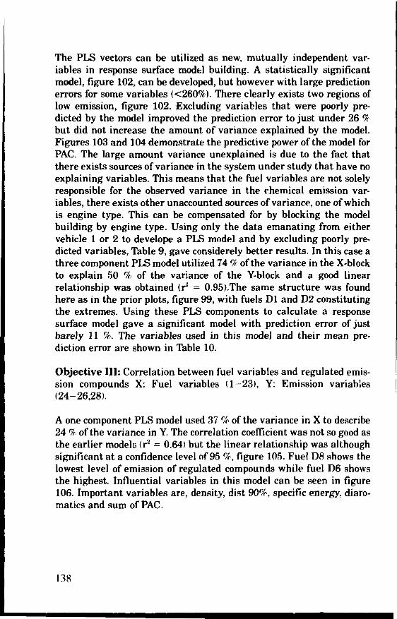
The PLS vectors can be utilized as new, mutually independent var-iables in response surface model building. A statistically significantmodel, figure 102, can be developed, but however with large predictionerrors for some variables (<260%). There clearly exists two regions oflow emission, figure 102. Excluding variables that were poorly pre-dicted by the model improved the prediction error to just under 26 %but did not increase the amount of variance explained by the model.Figures 103 and 104 demonstrate the predictive power of the model forPAC. The large amount variance unexplained is due to the fact thatthere exists sources of variance in the system under study that have noexplaining variables. This means that the fuel variables are not solelyresponsible for the observed variance in the chemical emission var-iables, there exists other unaccounted sources of variance, one of whichis engine type. This can be compensated for by blocking the modelbuilding by engine type. Using only the data emanating from eithervehicle 1 or 2 to develope a PLS model and by excluding poorly pre-dicted variables, Table 9, gave considerely better results. In this case athree component PLS model utilized 74 % of the variance in the X-blockto explain 50 % of the variance of the Y-block and a good linearrelationship was obtained (r2 = 0.95).The same structure was foundhere as in the prior plots, figure 99, with fuels Dl and D2 constitutingthe extremes. Using these PLS components to calculate a responsesurface model gave a significant model with prediction error of justbarely 11 %. The variables used in this model and their mean pre-diction error are shown in Table 10.

Objective III: Correlation between fuel variables and regulated emis-sion compounds X: Fuel variables (1-23), Y: Emission variables(24-26,28).

A one component PLS model used 37 r/r of the variance in X to describe24 % of the variance in Y. The correlation coefficient was not so good asthe earlier models (r2 = 0.64) but the linear relationship was althoughsignificant at a confidence level of 95 %, figure 105. Fuel D8 shows thelowest level of emission of regulated compounds while fuel D6 showsthe highest. Influential variables in this model can be seen in figure106. Important variables are, density, dist 90%, specific energy, diaro-matics and sum of PAC.

138

Table 9. Poorly predicted variables

Variable no

41.44.45.46.48.54.55.56.57.58.59.60.61.

Table 10. Mean

Objective IIVariable

24.25.26.27.28.29.30.31.32.33.34.35.36.37.38.39.40.42.43.47.

Prediction Error (%)

HCCONO,CO,ParticlesFuel consumptionSOFSO4FormaldehydeAcetaldehydeAcroleinMeta-acroleiniso-ValeraldehydeBenzeneTolueneEthenePropeneFluoranthene partPyrene partSum of PAC part

Name

Phenanthrene part2-methyl-pyrene partCyclopenta(cd)pyrene partBenzo(a)pyrene part1-nitro-Pyrene partPhenanthrene PUFFluoranthene PUFPyrene PUF2-methyl-pyrene PUFCyclopenta(cd)pyrene PUFBenzo(a)pyrene PUFSum of PAC PUF1-nitro-Pyrene PUF

Prediction Error

6.97.82.11.46.31.39.80

29.712.06.14.3

15.19.0

19.64.96.8

22.927.023.6

139

Objective IV: Correlation between fuel variables and unregulatedemission compounds: Fuel variables (1-23), Y: Emission variables(27,29-48).

A one component PLS model used 44 % of the variance in X to describe29 7c of the variance in Y. The correlation coefficient was significantlybetter (r2 = 0.90 for vehicle 1) and fuels Dl and D2 show the lowestlevel of emission, figure 107 and 108. Influential variables in thismodel can be seen in figure 109 for vehicle 1 and in figure 110 forvehicle 2. Important variables are, dist 90%, FBP, triaromatics and sumofPAC.

Objective V: Correlation between fuel variables and biological var-iables X: Fuel variables (1 -23), Y: Biological variables (49 53,62-66)

A four component PLS model used 89% of the variance in X to describe76% of the variance in Y. Influential variables in this model can be seenin figures 111 and 112. A good linear relationship was obtained be-tween blocks (r2 = 0.81), with essentially the same structure as inearlier plots, figure 113, with fuel blends Dl and D6 at the extremes.Using the PLS components to generate response surface models in-dicates two regions, as seen earlier, where effect/emission is at thelowest level, figure 114. These statistically significant models haveprediction errors as in Table 11. Important variables are, dist 90%, FBP,specific energy, total aromatics, triaromatics and sum of PAC.

Table 11. Mean Prediction Error {%)

Objective VVariable

49.50.51.52.53.62.63.64.65.66.

TA98-S9 part.TA98+S9 part.TA100-S9part.TA100+S9 part.TCDD part.TA98-S9 PUFTA98+S9 PUFTA100-S9 PUFTAI00+S9PUFTCDD PUF

Prediction Error

52.042.056.643.990.441.475.265.235.489.7

140

Objective VI: Correlation between emission variables and biologicalvariables X: Emission (24-48, 54-61), Y: Biological variables (49-53,62-66).

A four component PLS model uses 62% of the variance in X to describe77% of the variance in Y. The influence of the different variables on themodel can be seen in figures 115 and 116. Plots of this model show aslighlty different structure with fuel blend D6 as the extreme at higheffect but with fuel blend D2 as the extreme at low effect, figure117,instead of Dl as in earlier models. The linear relationship betweenblocks is also good in this model (r2 = 0.85). Response surface modelingof the PLS components gave a model with a mean prediction error of89% , figure 118, each variable's prediction error shown in Table 12.Important emission variables in the particulate and semivolatile phaseare: fluoranthene, pyrene, 2-methylpyrene and sum of PAC.

Table 12. Mean Prediction Error (%)

Variable

49.50.51.52.53.62.63.64.65.66.

TA98-S9 part.TA98+S9 part.TA100-S9 part.TA100+S9 part.TCDD part.TA98-S9 PUFTA98+S9 PUFTA100-S9 PUFTA100+S9 PUFTCDD PUF

Prediction Error

66.958.263.950.3

194.9103.8155.375.747.077.5

Objective VII: Correlation of Ames test to TCDD receptor test X:Ames test (49-55), Y: TCDD receptor test (53, 66).

Establishing i predictive relationship between these blocks of data byPLS was proven to be impossible, as can be seen in figure 119. Thevariation observed between objects approaches random variation andhence is not meaningful to model.

141

A&4 ConclusionsIn summing up the results of this study it can be observed that thereexists a quantifiable relationship between the variables of the fuelblends and the variables of the chemical emission and their biologicaleffect. Fuel blend D6 has extremely high emission, ranking highest inboth chemical and biological effect. Fuel blends Dl and D2 show thelowest emission in almost all objectives. Light grade diesel blend wasplaced in the middle in the range of emission. It was also found possibleto determine the importance of the individual composition parametersof the fuel blends in respect to their effect on the emission. Thus,Important fuel parameters: density, dist 909c, FBP, specific energy, totalaromatics, diaromatics, triaromatics and PAC content, has a greatimpact on the emission. On the other hand, the sulfur content of thefuel shows no significant contribution to the emission, except for regu-lated emission compounds. The addition of the igniter has also nonoticeable influence on the emission.

It was furthermore found possible to develope predictive models for sixof the seven objectives. Also, utilizing the above mentioned approach ofleaving out a portion of the data for use as a test-set afforded a means oftesting the developed models.

The model developed for objective II showed large prediction errors,especially for PAC and it also explains only a small portion of thevariance in PAH content of the emission. This indicates that the var-iation in PAC content in the emission is largely unaccounted for by themodel. For objective VII it was found to be impossible to develope apredictive model. This may be due to the different modes of action thatthe respective test procedures are a measure of.

A:2.5 ReferencesSharaf M., Illman D. and Kowalski B., "Chemometrics", Wiley, New York,J986.

Wold S., Cross-validatory estimation of the number of components in factorand principal components models. Technometrics, 20, 397, 11978).

Wold H., .Soft modelling: The basic design and some extcntions. In: Systemsunder Indirect Obsevations II. Edited by: KG. Joreskog and H. Wold. NorthHolland Publishing Co. Amsterdam, 1-54, 1982

142

PC 2 C 21 v.i

8

6PC 1 ( 45 x)

DIESEL CLASS N098

Figure 92. A two principal component scores plot of the fuel variables. Thepercentage for each principal component indicates how much of the variance isexplained by that component.

IB

5 in23 22

21• 4

i 8 If,

BETA 214

BETA 1

11

DIESEL CLASS FW9B

Figure 93. The loadings plot shows all the variables (bulk properties andchemical composition of the fuel blends) which have contributed to the princi-pal component plot in figure 1. Variables very far from origin contribute mostto the separation.

143

4<U2)4JJJ2)

2<U2)

2(U2)

PC 2 ( 29 /.)

1«U2)UZ>1<7<U2)

7#2> |S<U2)2(U2)• • 51U2)

5^02)

78<U2)

9CU2)

6(U2) 6(U2)

DIESEL CLASS N099

24J.V1)4<U1)8(U1>

BtVlWfi 1CW>

PC 1 < 2 3 y.)7(U1)

fe(Ul)

• I

Figure 94. A two principal component scores plot of the emission data. Thepercentage for each principal component indicates how much of the variance isexplained by that component. VI: Vehicle 1; V2: Vehicle 2.

EMISSION IZZ/.1

PLS 1 ( 49DIESEL CLASS NO1FOR PLS-COffPONENT NO 1 :XXXXXXXXXXXXXXXXXXXXXXXXCONFIDENCE LEVEL 95 v. AT 22 itREGRESSIONSCOEFF. K= 1.83 •/- .1293CORRELATIONSCOEFF. R= .96

Figure 95. A PLS regression model of different fuel blends (fuel D1-D9) forvehicle 1 where the x-axis is the PLS component XI (representing the fuelvariables, no.l -23) and the y-axis is the PLS-component Yl (representing theemission variables, no. 24-66». The percentage within the brackets indicateshow much of the variance is explained by that PLS component.

144

-01 - LOADINGS

-0.21 2 3 4 5 6 7 8 9 10 12 14 16 18 20 22

11 13 15 17 19 21 23

VARIABLE NO

Figure 96. The contribution (i.e. the loadings of the model) of each cf the fuelvariables (1- 23) for the correlation to emission data, vehicle 1. The greater theheight of a bar, either in positive (the response increases with increasing valueof the variable) or negative direction (the response increases with decreasingvalue of the variable), the greater the contribution of the variable to the model.The lines indicate, for each variable, the standard deviation of the modelresiduals (model-noise) at 95 % confidence level.

22 * Y

EMISSION ( Z l z )

DIESEL CLASS N02FOR PLS-COtlPONENT NO 1 :xxxxxxxxxxxxxxxxxxxxxxxxCONFIDENCE LEVEL 95 V. ATRIGRESSIOMSCOEFF. K= .96CORRELATIONSCOEFF. R= .94

PLS 1 ( 44 v.t

22 df•/- .1521

Figure 97. A PLS regression model of different fuel types (D1-D9) for vehicle 2where the x-axis is the PLS-component XI (representing the fuel variables,var no 1-23) and the y-axis is the PLS-component Yl (representing theemission variables, var no 24-66). The percentage within the brackets in-dicates how much of the variance is explained by that PLS-component.

145

LOADINGS

-0.21 2 3 4 5 6 7 8 9 10 12 14 16 18 20 22

11 13 15 17 19 21 23VARIABLE NO

Figure98. The contribution (i.e. the loadings of the model) of each of the fuelvariables (1—23) for the correlation to emission data (vehicle 2). The greaterthe height of a bar, either in positive (the response increases with increasingvalue of the variable) or negative direction (the response increases with de-creasing value of the variable), the greater the contribution for the variable inthe model. The lines indicate, for each variable, the standard deviation of themodel residuals at the 95 % confidence level.

CHEMICAL EMISSION

( 21 /.)

DIESEL CLASS NO11FOR PLS-COHPOMENT NO 1 :XXXXXXXXXXXXXXXXXXXXXXXXCONFIDENCE LEVEL 95 /. ATREGRESSIONSCOEFF. K= .87CORRELATIOHSCOEFF. R= .96

ZZ df*'- .1118

Figure 99. A PLS regression model of different fuel types (fuel D1-D9) forvehicle 1 where the x-axis is the PLS component XI (representing the fuelvariables, no.l -23) and the y-axis is the PLS-component Yl (representing thevariables of chemical emission, no 24-48, 54 61). The percentage within thebrackets indicates how much of the variance is explained by that PLS-compo-nent.

146

-0.1 - LOADINGS

-021 2 3 4 5 6 7 8 9 10 12 14 16 16 20 22

11 13 15 17 19 21 23

VARIABLE NO

Figure 100. The contribution (i.e. the loadings of the model) of each of the fuelvariables (1-23) for the correlation to chemical emission (vehicle 1). Thegreater the height of a bar, either in positive (the response increases withincreasing value of the variable) or negative direction (the response increaseswith decreasing value of the variable), the greater the contribution for thevariable in the model. The lines indicate, for each variable, the standarddeviation of the model residuals at the 95 % confidence level.

0.1 -

_<J1 , — LOADINGS

-0.224 26283032343638404244464B505254565B60G26466

2527293133363739 4143454749 5153555799616366VARIABLE NO

Figure 101. The contribution (i.e. the loadings of the model) of each of thechemical emission variables (24-48, 54-61) for the correlation to fuel var-iables (vehicle 1). The greater the height of a bar, either in positive (theresponse increases with increasing value of the variable) or negative directionI the response increases with decreasing value of the variable), the greater thecontribution for the variable in the model. The lines indicate, for each var-iable, the standard deviation of the model residuals at the 95 % confidencelevel.

147

SURFACE PLOT OF CLASS NO 11AS A FUNCT. OF CMBI. B1ZSSI0N

18

i

-a» *-- 8

X2 (FUEL WAR.)

- 6

PLS X I (FUEL WAR. >- 7

Figure 102. Response surface plot of the PLS model: Chemical emission (PLScomponent YD as a function of the values of the fuel variables IPI.S compo-nents XI and X2)

148

PREDICTED OF VARIABLE 42

R= .91 MID K= .77OBSERVED OF VARIABLE 42

Figure 103. Predicted values of variable 42 (fluoranten) from the PLS modelversus the actual values.

PREDICTED OF VARIABLE 4 7

R= .95 AND K= .95OBSERVED OF VARIABLE 47

Figure 104. Predicted values of variable 47 (total amount of PAH) from thePLS-model versus the actual values.

149

REGULATED COUP. <24x>

T L S I ( 37 * )

DIESEL CLASS NO4FOR PLS-COtlPONENT NO 1 :XXXXXXXXXXXXXXXXXOOOOCXXCONFIDENCE LEVEL 95 'x AT Z2 dfREGRESSIONCCOEFF. K- .33 •/- .1181CORRELATIONSCOEFF. R= .9

Figure 105. A PLS regression model of different fuel types (D1-D9) for vehicle2 where the x-axis is the PLS-component XI (representing the fuel variables,var. no.1-23) and the y-axis is the PLS-component Yl (representing theregulated compounds, vars. no.24, 25, 26 and 28). The percentage within thebrackets indicate how much of the variance is explained by that PLS-compo-nent.

LOADINGS

1 2 3 4 5 6 7 8 9 10 12 14 16 18 20 2211 13 15 17 19 21 23

VARIABLE NO

Figure 106. The contribution (i.e. the loadings of the model) of each of the fuelvariables (1-23) for the correlation to regulated compouds (vehicle 2). Thegreater the height of a bar, either in positive (the response increases withincreasing value of the variable) or negative direction (the response increaseswith decreasing value of the variable), the greater the contribution for thevariable in the model. T-e lines indicate, for each variable, the standarddeviation of the model residuals at the 95 % confidence level.

150

UNREGULATED COW (29x>

PLS 1 < 44 X)

DIESEL CLASS N05FOR PLS COMPONENT NO 1 :xxxxxxxxxxxxxxxxxxxxxxxxCONFIDENCE LEVEL 95 X AT 22 dfREGRESS IOKSCOEFF. K= .69 */- .6962CORRELATIONSCOEFF. R= .95

Figure 107. A PLS regression model of different fuel types (fuel D1-D9) forvehicle 1 where the x-axis is the PLS component XI (representing the fuelvariables, var. no.l -23) and the y-axis is the PLS-component Yl (representingthe unregulated compounds, var. no. 27, 29-48). The percentage within thebrackets indicates how much of the variance is explained by that PLS compo-nent.

UNREGULATED COHP <2»z)

PLS 1 ( 44 X)DIESEL CLASS N06FOR PLS-COHPONENT NO 1 :XXXXXXXXXXXXXXXXXXXXXXXXCONFIDENCE LEVEL 95 X AT 22 dfREGRESS I0NSCOEFF. K= .64 •/- .1556CORRELATIONSCOEFF. R= .87

Figure 108. A PLS regression model of different fuel blends (fuel D1-D9) forvehicle 2 where the x-axis is the PLS component XI (representing the fuelvariables, var. no.l -23) and the y-axis is the PLS-component Yl (representingthe unregulated compounds, var. no.27, 29-48). The percentage within thebrackets indicates how much of the variance is explained by that PLS compo-nent.

151

-0.1 - LOADINGS

-021 2 3 4 5 6 7 8 9 10 12 14 16 18 20 22

11 13 15 17 19 21 23VARIABLE NO

Figure 109. The contribution (i.e. the loadings of the model) of each of the fuelvariables (1-23) for the correlation to unregulated compounds (vehicle 1). Thegreater the height of a bar, either in positive (the response increases withincreasing value of the variable) or negative direction (the response increaseswith decreasing value of the variable), the greater the contribution for thevariable in the model. The lines indicate, for each variable, the standarddeviation of the model residuals at the 95 % confidence level.

-0.1

-0.2

LOADINGS

1 2 3 4 5 6 7 8 9 10 12 14 16 18 20 2211 13 15 17 19 21 23

VARIABLE NO

Figure 110. The contribution (i.e. the loadings of the model) of each of the fuelvariables (1 -23) for the correlation to unregulated compounds (vehicle 2). Thegreater the height of a bar, either in positive (the response increases withincreasing value of the variable) or negative direction (the response increaseswith decreasing value of the variable), the greater the contribution for thevariable in the model. The lines indicate, for each variable, the standarddeviation of the model residuals at the 95 % confidence level.

152

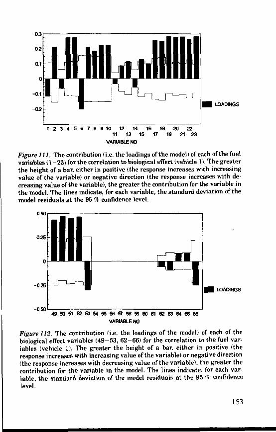
tiiuiuiiLOADINGS

1 2 3 4 5 6 7 8 9 10 12 14 16 18 20 2211 13 15 17 19 21 23

VARIABLE NO

Figure 111. The contribution (i.e. the loadings of the model) of each of the fuelvariables i 1 -23) for the correlation to biological effect (vehicle 1). The greateTthe height of a bar, either in positive (the response increases with increasingvalue of the variable) or negative direction (the response increases with de-creasing value of the variable), the greater the contribution for the variable inthe model. The lines indicate, for each variable, the standard deviation of themodel residuals at the 95 % confidence level.

0.50

0.25 -

-0.25 -

-0.50

LOADINGS

51525354555657585960616263646666VARIABLE NO

Figure 112. The contribution (i.e. the loadings of the model) of each of thebiological effect variables (49-53, 62-66) for the correlation to the fuel var-iables (vehicle 1). The greater the height of a bar, either in positive (theresponse increases with increasing value of the variable) or negative direction(the response increases with decreasing value of the variable), the greater thecontribution for the variable in the model. The lines indicate, for each var-iable, the standard deviation of the model residuals at the 95 °!r confidencelevel.

153

BIOLOGICAL EFFECT

97 •

DIESEL CLASS HO1ZFOR PLS-COHPONENT HO 1 :xxxxxxxxxxxxxxxxxxxxxxxxCONFIDENCE LEVEL 95 v. ATREGRESSIOHSCOEFF. K= .58CORRELATIONSCOEFF. R= .9

PLS 1 ( 44 V.)

22 df•/- .1245

Figure 113. A PLS regression model of different fuel blends (fuels D1-D9) forvehicle 1 where the x-axis is the PLS component XI (representing the fuelvariables, var. no. 1-23) and the y-axis is the PLS-component Yl (repre-senting the variables of biological effect, var. no.49-53, 62-66). The percent-age within the brackets indicates how much of the variance is explained bythat PLS-component.

154

RESPONSE SURFACE PLOT OF CLASS NO ISAS A FUNCT. OF BIOLOG. EFFECT

- 1 6

- 6

PLS XI (FUEL VARIABLES)-4 .3

Figure 114. Response surface plot of the PLS model: Biological effect (PLScomponent Yl) as a function of the values of the fuel variables (PLS compo-nents XI and X2).

155

lOADMQS

-0.2^ 2 6 2 8 3 0 3 2 3 4 3 6 3 8 4 0 4 2 4 4 4 6 4 8 5 5 5 7 5961

2 5 2 7 2 9 3 1 3 3 3 5 3 7 3 9 41 43 45 47 54 56 58 60VARIABLE NO

Figure 115. The contribution (i.e. the loadings of the model) of each of thechemical emission variables (24-48,54-61) for the correlation to biologicaleffect (vehicle 1). The greater the height of a bar, either in positive (theresponse increases with increasing value of the variable) or negative direction(the response increases with decreasing value of the variable), the greater thecontribution for the variable in the model. The lines indicate, for each var-iable, the standard deviation of the model residuals at the 95 % confidencelevel.

0.50

025

-0.25

-0.50

LOADINGS

50 51 52 53 62 63

VARIABLE NO

64 65

Figure 116. The contribution (i.e. the loadings of the model) of each of thebiological effect variables (49-53, 62 66) for the correlation to the chemicalemission variables (vehicle 1). The greater the height of a bar, either inpositive (the response increases with increasing value of the variable) ornegative direction (the response increases with decreasing value of the var-iable), the greater the contribution for the variable in the model. The linesindicate, for each variable, the standard deviation of the model residuals at the95 r/t- confidence level.

156

BIOLOGICAL EFFECT

DIESEL CLASS N01&FOR PLS-COnPONENT NO 1 :xxxxxxxxxxxxxxxxxxxxxxxxCONFIDENCE LEVEL 95 X ATREGRESSIONSCOEFF. K= .62CORRELATIONSCOEFF. R= .92

PLS 1 < 26 x)

22 it••- .1179

Figure 117. A PLS regression model of the different fuel blends (D1-D9) forvehicle 1 where the x-axis is the PLS-component XI (representing the chem-ical emission variables, var. no.24—48, 54-61) and the y-axis is the PLS-component Yl (representing the variables of biological effect, var. no.49-53,62-66). The percentage within the brackets indicates how much of the var-iance is explained by that PLS-component.

PflEDICTKD OF UAHIrtlll.K f.X

R= .98 AND K= .95OBSERVED OF VARIABLE 62

Figure 118. Predicted values of variable 62 (TA98-H9) from the PLS modelversus the actual values.)

157

TCDD

6S547

78521

8S527PLS 1 ( 40 x>

5SS34

2SS82»2S5817SS28

DIESEL CLASS H017FOR PLS-COHPONEHT NO 1 :»OOOOOOOOOOOOOOOOCXXXXXXCONFIDEHCE LEVEL 95 z AT 22 dfREGRESSIOHSCOEFF. K= .38 •/- .1897C0RRELATI0NSCOEFF. H= .66

Figure 119. A PLS regression model of different the fuel blends (no.1-9) forvehicle 1 where the x-axis is the PLS-component XI (representing the var-iables of Ames-test, var. no.49-52, 62-65) and the y-axis is the PLS-compo-nent Yl (representing the variables of TCDD-receptor, var. no.53 and 66). Thepercentage within the brackets indicates how much of the variance is ex-plained by that PLS-component.

J58

This report presents an investigation of theemissions from eight diesel fuels with differ-ent sulphur and aromatic content. A busand a truck were used in the investigation.Chemical analysis and biological testinghave been performed.

The aim of this project was to find a "good"diesel fuel which can be used in urban ar-eas. Seven of the fuels were meant to besuch fuels.

It has been confirmed in this study thatthere exists a quantifiable relationship be-tween the variables of the diesel fuel blendsand the variables of the chemical emissionsand their biological effects.

ISSN 0282-7298ISBN 91-620-3968-7Kommentus 158 1027Graphic SystemsStockholm 1991