Impact damping and friction in non-linear mechanical systems ...

Impact damping and friction in non-linear mechanical systems with

combined rolling-sliding contact

Dissertation

Presented in Partial Fulfillment of the Requirements for the Degree Doctor of Philosophy

in the Graduate School of The Ohio State University

By

Sriram Sundar, B. E.

Graduate Program in Mechanical Engineering

The Ohio State University

2014

Dissertation Committee:

Prof. Rajendra Singh, Advisor

Prof. Dennis A Guenther

Prof. Ahmet Kahraman

Prof. Vishnu Baba Sundaresan

Dr. Jason T Dreyer

Copyright by

Sriram Sundar

2014

ii

ABSTRACT

This research is motivated by the need to have a better understanding of the non-

linear contact dynamics of systems with combined rolling-sliding contact such as cam-

follower mechanism, gears and drum brakes. Such systems, in which the dominant

elements involved in the sliding contact are rotating, have unique interaction among

contact mechanics, siding friction and kinematics. Prior models used in the literature are

highly simplified and do not use contact mechanics formulation hence the dynamics of

the system are not well understood. The main objective of this research is to gain a

fundamental understanding of the non-linearities and contact dynamics of such systems,

for which a cam-follower mechanism is used as an example case. Specifically, the non-

linearities, impact damping and coefficient of friction are analyzed in this study. The

problem is examined using a combination of analytical, experimental, and numerical

methods.

First, the various non-linearities (kinematic, dry friction, and contact) of the cam-

follower system with combined rolling-sliding contact are investigated using the Hertzian

contact theory for both line and point contacts. Alternate impact damping formulations

are assessed and the results are successfully compared with experimental results as

available in the literature. The applicability of the coefficient of restitution model is also

critically analyzed. Second, a new dynamic experiment is designed and instrumented to

iii

precisely acquire the impact events. A new time-domain based technique is adopted to

accurately calculate the system response by minimizing the errors associated with

numerical integration. The impact damping force is considered in a generalized form as a

product of damping coefficient, indentation displacement raised to the power of damping

index, and the time derivative of the indentation displacement. A new signal processing

procedure is developed (in conjunction with a contact mechanics model) to estimate the

impact damping parameters (damping coefficient and index) from the measurements by

comparing (on the basis of three residues) them to the results from the contact mechanics

model. Also few unresolved issues regarding the impact damping model are addressed

using the experimental results. Third, the coefficient of friction under lubrication is

estimated using the same experimental setup (operating under sliding conditions). A

signal processing technique based on complex-valued Fourier amplitudes of the measured

forces and acceleration is proposed to estimate the coefficient of friction. An empirical

relationship for the coefficient of friction is suggested for different surface roughnesses

based on a prior model under lubrication. Possible sources of errors in the estimation

procedure are identified and quantified.

Some of the major contributions of this research are as follows. First, impact

damping model was determined experimentally and related unresolved issues were

addressed. Second, coefficient of friction for a cam-follower system with point contact

under lubricated condition was estimated. Finally, better understandings of the effect of

non-linearities and shortcomings of coefficient of restitution formulation are obtained.

iv

Dedication

To the lotus feet of my spiritual master

His Holiness Sri Rangaraamaanuja Mahaadesikan

v

ACKNOWLEDGEMENTS

First, I would like to thank my advisor, Prof. Rajendra Singh, for his patience and

guidance throughout my graduate study. His tremendous experience and knowledge has

been helped me overcome the difficulties faced during this process. I also would like to

express my deepest appreciation to Dr. Jason Dreyer for his extremely valuable support

in the experimental work and many technical discussions. I would like to thank my

committee members, Prof. Guenther, Prof. Kahraman and Prof. Sundaresan for their time

to review my work. I also would like to thank Caterina Runyon-Spears for her careful

reviews of this work and all the members of Acoustics and Dynamics Lab for their

providing with an amicable atmosphere over the past four years. Special thanks to

Laihang for helping me record the experimental data. I would like to thank the Vertical

Lift Consortium, Inc., Smart Vehicles Concept Center (www.SmartVehicleCenter.org)

and the National Science Foundation Industry/University Cooperative Research Centers

program (www.nsf.gov/eng/iip/iucrc) for partially supporting this research.

I am most grateful to my parents, brother, fiancée and other family members for

their constant faith, support and patience. I would like to thank all my friends especially,

Adarsh, Ranjit, Sriram, Saivageethi and Darshan who made my graduate life, away from

home, a memorable one. Also a special thanks to Sriram’s mom, for her mother-like care

during all her visits in these four years.

vi

VITA

December 25, 1985……………………………… Born - Chennai, India

2003……………………………………………… B. E. Mechanical Engineering

Anna University,

Chennai, India

2009 – Present…………………………………… University Fellow/ SVC Fellow

Graduate Research Associate

The Ohio State University

Columbus, OH

PUBLICATIONS

1. S. Sundar, J. T. Dreyer and R. Singh, Rotational sliding contact dynamics in a non-

linear cam-follower system as excited by a periodic motion, Journal of Sound and

Vibration, (2013).

2. S. Sundar, J. T. Dreyer and R. Singh, Effect of the tooth surface waviness on the

dynamics and structure-borne noise of a spur gear pair, SAE Technical Paper 2013-01-

1877, 2013, SAE Noise and Vibration Conference.

FIELDS OF STUDY

Major Field: Mechanical Engineering

Main Study Areas: Mechanical Vibrations, Nonlinear Dynamics, Sliding Contact

Systems, Contact Mechanics.

vii

TABLE OF CONTENTS

Page

ABSTRACT……………………………………………………………...……………… ii

DEDICATION…………………………………………………………………………... iv

ACKNOWLEDGEMENTS……………………………………………………...………. v

VITA……………………………………………………………………………..…….... vi

LIST OF TABLES ............................................................................................................ xi

LIST OF FIGURES ........................................................................................................ xiii

LIST OF SYMBOLS ...................................................................................................... xix

CHAPTER 1: INTRODUCTION....................................................................................... 1

1.1 Motivation ........................................................................................................ 1

1.2 Literature review............................................................................................... 2

1.3 Problem formulation......................................................................................... 4

References for Chapter 1 ..................................................................................... 10

CHAPTER 2: ROTATIONAL SLIDING CONTACT DYNAMICS IN A NON-LINEAR

CAM-FOLLOWER SYSTEM AS EXCITED BY A PERIODIC MOTION………..… 16

2.1 Introduction .................................................................................................... 16

2.2 Problem formulation………………………………………………………... 17

2.3 Analytical model……………………………………………………….…… 20

2.3.1 Relationship between the coordinate systems……………….……. 20

viii

2.3.2 Equations of motion………………………………………………. 21

2.3.3 Static equilibrium and linearized natural frequency……………… 24

2.3.4 Contact damping and dry friction models……………………….... 25

2.4 Examination of the contact non-linearity and alternate damping models…... 27

2.5 Assessment of the coefficient of restitution (ξ) concept……………………. 33

2.6 Study of the line and point contact models in the sliding contact regime….. 38

2.7 Analysis of the friction non-linearity……………………………………….. 40

2.7.1 Effect of direction………………………………………………… 40

2.7.2 Dynamic bearing and friction forces……………………………… 40

2.8 Study of kinematic non-linearity…………………………………………… 47

2.9 Conclusion………………………………………………………………….. 49

References for Chapter 2 ..................................................................................... 53

CHAPTER 3: ESTIMATION OF IMPACT DAMPING PARAMETERS FROM TIME-

DOMAIN MEASUREMENTS ON A MECHANICAL SYSTEM……………...…….. 58

3.1 Introduction…………………………………………………………...…….. 58

3.2 Problem formulation……………………………………………………...… 59

3.3 Design of the laboratory experiment and instrumentation………………….. 61

3.4 Analytical model……………………………………………………………. 62

3.4.1 Kinematics of the system……………………………………….… 62

3.4.2 Non-contact regime……………………………………………..… 65

3.4.3 Contact regime…………………………………………………..... 66

3.5 Estimation of the impact damping parameters (β and n)…………………… 68

ix

3.5.1 Time-domain based technique to estimate the system response….. 68

3.5.2 Signal processing procedure to estimate β and n…………………. 70

3.6 Error and sensitivity analyses on the estimation procedure……………….... 72

3.6.1 Error analysis…………………………………...………………… 72

3.6.2 Sensitivity analysis……………………………………..…………. 76

3.7 Estimation of the impact damping from the measurements………………… 79

3.8 Equivalent coefficient of restitution………………………………………… 84

3.8.1 Governing equation………………………………………..……… 84

3.8.2 Estimation of the equivalent ξ model……………………...……… 86

3.8.3 Justification of the estimated impact damping parameters……….. 90

3.9 Conclusion………………………………………………………………….. 91

References for Chapter 3……………………………………………………….. 93

CHAPTER 4: ESTIMATION OF COEFFICIENT OF FRICTION FOR A

MECHANICAL SYSTEM WITH COMBINED ROLLING-SLIDING CONTACT

USING VIBRATION MEASUREMENTS………………………………………..…… 98

4.1 Introduction………………………………………………………………..... 98

4.2 Problem formulation……………………………………………………...… 99

4.3 Contact mechanics model……………………………………………...….. 102

4.4 Experiment for the determination of µ………………………………….…. 107

4.5 Identification of system parameters…………………………………..…… 108

4.5.1 Identification of geometrical parameters…………………..…..... 108

x

4.5.2 Identification of the modal damping ratio………………………. 113

4.6 Signal processing technique to estimate µ……………………………….... 114

4.7 Experimental results and friction model…………………………………... 119

4.8 Potential sources of error in the estimation of µ…………………...……… 123

4.9 Conclusion…………………………………………………………...……. 130

References for Chapter 4 ................................................................................... 132

CHAPTER 5: CONCLUSION……………………………………………………...… 137

5.1 Summary ………………………………………………………………..… 137

5.2 Contributions …………………………………………………………...… 138

5.3 Future work ……………………………………………………………..… 139

References for Chapter 5 ................................................................................... 141

BIBLIOGRAPHY…………………………………………………………………..…. 142

xi

LIST OF TABLES

Table Page

3.1 Comparison of average residues per impact (Λ1, Λ2 and Λ3) using two simulations

(S1 and S2) with 1 2 2.524.7 GNsmS Sβ β −= = and 1 2 1.5S S

n n= = ………………….. 75

3.2 Comparison of normalized average residues per impact (1 2 3, andΛ Λ Λ ) using

simulation S2 ( 2 2.524.7 GNsmSβ −= and 2 1.5S

n = ) with e/rc = 0.2 and Ωc = 16 Hz.

a) For different values of 1Sβ in the proximity of 2Sβ with constant value of

1 2S Sn n= .b) For different values of 1S

n in the proximity of 2Sn with constant value

of 1 2S Sβ β= ………………………...………………………………………...…. 78

3.3 Error in the estimation of ξ model using time histories from simulation S3

( )3 0.8s/mSγ = ………………………………………………………………...….. 88

4.1 Comparison of measurements and predictions (from the contact mechanics model)

with µ = 0.51 and e/a = 0.116 at the harmonics of Ωc = 11.55 Hz…………....… 122

4.2 Error in the estimation of µ for the mechanical system with a circular cam for

different values of e at Ωc = 11.55 Hz………………………………………..…. 127

4.3 Error in the estimation of µ for the mechanical system with circular cam for

different cam speeds with e/a = 0.1…………………………………………...… 128

xii

4.4 Error in the estimation of µ for the mechanical system with an elliptic cam at Ωc =

8.33 Hz and e = 0.1 a…………………………………………………………..... 130

Figure

1.1

1.2

2.

2.2

2.3

2.4

2.5

Figure

1.1 Analytical model of typical cam

formulation

1.2 Cam-follower experiment designed

view of the cam

contact………………………………………………………………………………

2.1 Cam-follower system in the general state where a non

model, k

2.2 Free body diagram of the follower in the sliding contact regime

2.3 Normalized d

Coulomb friction (Model I);

2.4 Comparison

mechanics

model C;

from literature [8];

2.5 Comparison of predicted

data at Ω

Analytical model of typical cam

formulation………………………………………………………

follower experiment designed

view of the cam-follower experiment built using a lathe; b) Closer view of the

contact………………………………………………………………………………

follower system in the general state where a non

kλ(ψi(t)), is employed

Free body diagram of the follower in the sliding contact regime

Normalized dry friction models (equations are given in Section


Comparison of r

rmsα

mechanics formulation with damping model A

model C; , damping model D;

from literature [8];

Comparison of predicted

data at Ωc = 155rpm.

LIST OF

Analytical model of typical cam

………………………………………………………

follower experiment designed

follower experiment built using a lathe; b) Closer view of the

contact………………………………………………………………………………


, is employed……………………………


ry friction models (equations are given in Section


r

rms and r

pα at lower speeds.

formulation with damping model A

, damping model D;

, prior analytical result from literature

Comparison of predicted ( )r tα

= 155rpm. Key: ,

xiii

LIST OF FIGURES

Analytical model of typical cam-follower system with contact mechanics

………………………………………………………

follower experiment designed to study the contact mechanics. a) Isometric


contact………………………………………………………………………………


……………………………



, Smooth

r

p at lower speeds.

formulation with damping model A

, damping model D; , damping model E;


( )t using different damping models with experimental

, contact mechanics formulation with damping model

FIGURES

follower system with contact mechanics

………………………………………………………

to study the contact mechanics. a) Isometric


contact………………………………………………………………………………


……………………………



, Smoothened Coulomb friction (Model II)

at lower speeds. (a)r

rmsα

formulation with damping model A; , damping model B;

, damping model E;


using different damping models with experimental

contact mechanics formulation with damping model


…………………………………………………………………



contact………………………………………………………………………………

follower system in the general state where a non-linear contact stiffness

………………………………………..

Free body diagram of the follower in the sliding contact regime…………

ry friction models (equations are given in Section 2.

ened Coulomb friction (Model II)

r

rms ; (b) r

pα . Key:

, damping model B;

, damping model E; , experimental result

, prior analytical result from literature [2.8]




…………...…..



contact………………………………………………………………………………

linear contact stiffness

…………..……...…….

……………...…

2.3.4). Key:

ened Coulomb friction (Model II)

. Key: , contact

, damping model B; , damping

, experimental result

[2.8]….…….....



Page


…..… 6



contact……………………………………………………………………………… 7

linear contact stiffness

….. 19

… 22

3.4). Key: ,

ened Coulomb friction (Model II)... 28

contact

, damping

, experimental result

... 31



2.6

2.7

2.8

2.9

2.10

A; , damping model B;

model E;

2.6 Comparison of experimental and analytical results for

domain comparison; (b) Frequency domain comparison. Key:

contact mechanics formulation with damping model D;

from Alzate et al.

2.7 Map of

model;

from Alzate et al.

technique (given in Section

2.8 Map of

mechanics formulation;

analytical results from Alzate et al.

energy balance technique (given in Section

2.9 Identification of contact domains based on

with e = 0.1

2.10 Comparison of

showing harmonics of

Key:

, damping model B;

model E; , prior experimental result from literature

Comparison of experimental and analytical results for



from Alzate et al. [2.8]

Map of r

pα vs. Ωc

, experimental results from Alzate et al.

from Alzate et al.

technique (given in Section

, ξ = 0.6………………………………………………………………..

Map of r

pα vs. Ωc

mechanics formulation;



, ξ = 1. ………………………………

Identification of contact domains based on

= 0.1rc………………………………

Comparison of spectra (with

showing harmonics of

, de-energizing system with line contact (

αɺɺ

, damping model B; , damping model C;

, prior experimental result from literature




[2.8]………………….

at lower speeds. Key:


from Alzate et al. [2.8];

technique (given in Section 2.4.2) with

………………………………………………………………..

over a broad range of speeds. Key:

mechanics formulation; , experimental results from Alzate et al.



………………………………


………………………………

spectra (with

showing harmonics of Ωc; (b) Spectra showing natural frequency of the system

energizing system with line contact (

xiv

, damping model C;





………………….…………………………….

at lower speeds. Key:


, prediction based on approximate energy ba

4.2) with ξ = 0.05;

………………………………………………………………..



analytical results from Alzate et al. [2.8];


………………………………


………………………………

spectra (with µm = 0.3, ζ

; (b) Spectra showing natural frequency of the system

energizing system with line contact (

, damping model C; , damping model D;


Comparison of experimental and analytical results for α



…………………………….

at lower speeds. Key: , predictions from

, experimental results from Alzate et al. [2.8]


= 0.05;

………………………………………………………………..



, prediction based on approximate

energy balance technique (given in Section 2.4.2) with

…………………………………………………………………

Identification of contact domains based on ks - Ωc mapping at a constant cam speed

……………………………………………………...

ζD

= 0.01 and


energizing system with line contact (lλ

, damping model D;

, prior experimental result from literature [2.8]…….

rα at Ωc = 155rpm


contact mechanics formulation with damping model D; , experimental result

…………………………….

, predictions from contact mechanics

[2.8]; , prior analytical results


, ξ = 0.2;

………………………………………………………………..

over a broad range of speeds. Key: , predictions from



4.2) with ξ = 0.2;

…………………………………

mapping at a constant cam speed

……………………...…………

and βD

= 4.25


lλ = 0.0016m,

, damping model D; , damping

…….………….

= 155rpm. (a) Time

domain comparison; (b) Frequency domain comparison. Key: , analytical

experimental result

……………………………..…………..

contact mechanics

, prior analytical results


= 0.2; , ξ = 0.4;

………………………………………………………………..…

, predictions from contact

, experimental results from Alzate et al. [2.8]; , prior


, ξ = 0.6;

………………………………….


…………...…..

s/m). (a) Spectra


= 0.0016m, Ωc = 300 rpm

, damping

…………... 32

. (a) Time

, analytical

experimental result

………….. 33

contact mechanics

, prior analytical results

lance

= 0.4;

… 37

contact

, prior


= 0.6;

... 38


….. 42

(a) Spectra

; (b) Spectra showing natural frequency of the system.

= 300 rpm);

xv

, self-energizing system with line contact (lλ = 0.0016m, Ωc = -300 rpm);

, de-energizing system with point contact (Ωc = 300 rpm)……….……….. 43

2.11 Comparison of Fn(t) for different direction of cam rotation with line contact (lλ =

0.0016m, µm = 0.3, ζD

= 0.01 and βD

= 4.25 s/m). Key: , de-energizing (Ωc =

300 rpm); , self-energizing (Ωc = -300 rpm)…………………………….… 44

2.12 Comparison of relative sliding velocity vr(t) for two dry friction models of Fig. 2.3

(with Ωc = 50 rpm, e = 0.7rc , ζD

= 0.01 and βD

= 4.25 s/m). Key: , Coulomb

friction; , Smoothened Coulomb friction…………………….….………… 45

2.13 Comparison of forces for two dry friction models of Fig. 2.3 (with Ωc = 50 rpm, e =

0.7rc, ζD

= 0.01 and βD

= 4.25 s/m). (a) Nx(t); (b) Ff(t). Key: , Coulomb friction;

, Smoothened Coulomb friction……………………………………...……. 46

2.14 Comparison of relative sliding velocity vr(t) for two dry friction models of Fig. 2.3

(with ωc = 40 rpm, e = 0.7rc, ζD

= 0.01 and βD


friction; , Smoothened Coulomb friction………….………………………. 47

2.15 Comparison of forces for two dry friction models of Fig. 2.3 (with ωc = 40 rpm, e =

0.7rc, ζD

= 0.01 and βD

= 4.25 s/m). (a) Ff(t); (b) Nx(t). Key: , Coulomb friction;

, Smoothened Coulomb friction……………………………………..…….. 51

2.16 Comparison of spectra (with µm = 0.3, Ωc = 300 rpm, ζD

= 0.01 and βD

= 4.25

s/m). (a) Spectra showing harmonics of Ωc; (b) Spectra showing natural frequency

of the system. Key: , Non-linear system; , Linear system…….……. 52

3.1 Cam-follower experiment designed to determine impact damping parameters…. 61

3.2 Analytical contact mechanics model of the experiment shown in Fig. 3.1…….... 64

αɺɺ

xvi

3.3 Regimes of contact and impact for the system (with parameters given in section

3.6.1) via Ωc vs. e/rc. Key: , Operational points (with periodic impacts) selected

for the purpose of error analyses……………………………………………..….. 74

3.4 Comparison of hysteresis loops for single impacts during simulation S2 (

2 2.524.7 GNsmSβ −= and 2 1.5S

n = ) and simulation S1 ( 1 2S Sβ β= and 1 2S Sn n= )

given e/rc = 0.2 and Ωc = 16 Hz. Key: , Simulation S1; , Simulation

S2………………………………………………………………………………… 76

3.5 Time histories of the measured forces and acceleration with e/rc = 0.13 and Ωc =

14 Hz (with other parameters given in section 3.6.1). a) Normalized reaction force

along ˆx

e ; b) Normalized reaction force along ˆy

e ; c) Angular acceleration of the

follower………………………………………………………………….………. 81

3.6 Sample measured forces and acceleration during the contact sub-event from a

single impact from measurements shown in Fig. 3.5. a) Reaction forces; b)

Angular acceleration. Key: , Normalized reaction force along ˆx

e ; ,

Normalized reaction force along ˆy

e …………………………………….………. 82

3.7 Comparison of the hysteresis loops from measured data of Fig. 3.6 and simulation

S1 (using the impact damping model selected based on minimization of Λ1). Key:

, Measured; , Simulation S1 (with 1 -2.549.3 GNsmSβ = and

1 1.5S

n = )………………………………………………………………..……….. 83

3.8 Comparison of the hysteresis loops from measured data of Fig. 3.6 and simulation

S1 (using viscous damping model selected based on minimization of Λ1) Key:

xvii

, Measured; , Simulation S1 with viscous damping ( 1 0S

n = and

1 1.47 kNs/mSβ = )………………………………………………………….....… 85

3.9 Variation in estimated iξ (during different impacts) with b

iψɺ given e/rc = 0.10 and

Ωc = 18 Hz. Key: , Simulation S3 ( 3 0.8 s/mSγ = ) ; , Estimated ξ model

with γ = 0.799 s/m (using least square curve-fitting technique)…………..…….. 89

3.10 Variation in estimated iξ (during different impacts) with b

iψɺ for the experimental

data of Fig. 3.5. Key: , Experimental data for different impact; ,

Estimated ξ model with γ = 0.758 s/m (using least square curve-fitting technique).

…………………………………………………………………………………… 90

4.1 Example case: A mechanical system with an elliptic cam and follower supported by

a lumped spring (ks)………………………………………………………..……. 101

4.2 Free-body diagram of the follower; refer to Fig. 4.1 for the two coordinate

systems……………………………………………………………………..……. 106

4.3 Mechanical system experiment used to determine the coefficient of friction (µ) at

the cam-follower interface………………….……………………………..…….. 110

4.4 Classification of response regimes of the mechanical system with a circular cam in

terms of Ωc vs. e/a map with the parameters of section 4.5. Key: ,

Operational range of the experiment…………………………….………………. 112

4.5 Slide-to-roll ratio for the cam-follower system with e/a = 0.12 and Ωc = 11.55 Hz

and other parameters of section 4.5…………………………...……………...…. 113

4.6

4.7

4.8

4.9

4.10

4.6 Impulse experiment to determine the viscous damping ratio associated with the

lubricated contact regime. a) Experimental setup; b) Top view of the dowel pin

arrangement showing the three

4.7 Relative accelerance spectra in the vicinity of the system resonance. Key:

dry (unlubricated);

oil…………………………………………………………………………

4.8 Estimated

range) for the dry friction regime

ISO 32 oil;

pin with steel disk

4.9 Comparison of the modified Benedict

with friction values reported in the literature

for AGMA 4EP oil (

lubrication regime

Grunberg and Campbell

4.10 Classification of response regimes of a mechanical system with an elliptic cam in

terms of a

4.5. Key:

Impulse experiment to determine the viscous damping ratio associated with the



Relative accelerance spectra in the vicinity of the system resonance. Key:

dry (unlubricated);

…………………………………………………………………………

Estimated µ for different


ISO 32 oil; , dry contact

pin with steel disk [4.13]

Comparison of the modified Benedict


for AGMA 4EP oil (

lubrication regime),

Grunberg and Campbell

Classification of response regimes of a mechanical system with an elliptic cam in

terms of a Ωc – b/a

Key: , Operational range of simulation





dry (unlubricated); , lubricated with AGMA 4EP oil;

…………………………………………………………………………

for different Rm values and comparison with prior values (including the


, dry contact - iron pin with steel disk

[4.13]……………………

Comparison of the modified Benedict


for AGMA 4EP oil (EHL regime

), , Shon et al.

Grunberg and Campbell [4.34];


a map with e

, Operational range of simulation

xviii



point contacts. Key:


, lubricated with AGMA 4EP oil;

…………………………………………………………………………

values and comparison with prior values (including the

range) for the dry friction regime [4.13]. Key:

iron pin with steel disk

……………………

Comparison of the modified Benedict-Kelley model from the results of


EHL regime);

, Shon et al. [4.16]

; , Furey [4.35]


e = 0.1a and other parameter values given in section

, Operational range of simulation



point contacts. Key: , contact point…….……..



…………………………………………………………………………


. Key: , With AGMA 4EP oil;

iron pin with steel disk [4.13]

……………………………………………………

Kelley model from the results of

with friction values reported in the literature [4.16, 4.33

, Model for ISO 32 oil (

[4.16]; , , Xu and Kahraman

[4.35]……………………


and other parameter values given in section

, Operational range of simulation………………………



, contact point…….……..


, lubricated with AGMA 4EP oil; , lubricated with ISO 32

…………………………………………………………………………


, With AGMA 4EP oil;

[4.13]; , dry contact

………………………………

Kelley model from the results of

4.33 - 35]. Key:

, Model for ISO 32 oil (

, Xu and Kahraman

……………………



……………………



, contact point…….……..


, lubricated with ISO 32

…………………………………………………………………………..…….


, With AGMA 4EP oil; , With

, dry contact - copper

………………………………..…..

Kelley model from the results of Fig.

. Key: , Model

, Model for ISO 32 oil (mixed

, Xu and Kahraman [4.33]

…………………………..……



……………………...….



, contact point…….…….. 115

,

, lubricated with ISO 32

……. 116


, With

copper

….. 121

Fig. 4.8

, Model

mixed

[4.33];

…… 124



…. 129

xix

LIST OF SYMBOLS

List of symbols for Chapter 1

c Damping

F Dynamic force

k Stiffness

α Angular displacement of the follower

δ Indentation

κ Arbitrary constant

µ Coefficient of friction

η Arbitrary constant

Θ Angular displacement of the cam

Subscripts

k Stiffness

s Spring

λ Contact

Operators

, First and second derivative with respect to time


c damping

d Length from cam pivot point to the point where follower spring base

xx

E Cam pivot point

e Eccentricity or runout

)ˆ,ˆ( yx ee Fixed co-ordinate system along vertical and horizontal directions

f Frequency

F Dynamic force

h Non-linear function (for Jacobian method)

G Center of gravity point

I Mass moment of inertia

J Jacobian matrix

)ˆ,ˆ( ji Moving co-ordinate system (with being parallel to the follower)

k Translational stiffness

L Length

l Length of line contact

N Bearing reaction force

n Impact damping index

O Contact stiffness location

P Follower pivot point

Q Origin of , coordinate system

r Radius of the cam

t Time

T Kinetic energy

u Velocity of the contact point along iɵ

v Sliding velocity

V Potential energy

w width

Y Young’s modulus

xxi

α Rotation of the follower from the horizontal in both the coordinate systems

β Impact damping factor

ξ Coefficient of restitution

∆ Change

χ Moment arm of the normal force on the follower about the pivot point.

Ξ State space vector

( ),i j

ψ ψ Translational displacement variables for the cam in the )ˆ,ˆ( ji coordinate system

ε Generalized state space variable

Ω Angular velocity

ω Angular frequency of oscillation

Θ Angular displacement variable of the cam in the (, ) coordinate system

θ Angular displacement variable of the cam in the (,) coordinate system


σ Regularizing factor for smoothing (hyperbolic tangent) function

ν Poisson’s ratio

ζ Damping ratio

ϑ Natural frequency

Subscripts

b Follower

c Cam

e Equivalent

f Friction

l Linearized

m Static

n Normal

λ Denotes contact parameters

xxii

p Peak to peak

r Relative

rms root-mean-square

s Spring

x, y horizontal and vertical directions

Superscripts

a After impact

b Before impact

c Out of contact

0 Zero displacement state

i In contact

P Denotes moment (or) moment of Inertia about the follower pivot point

r Residual

u uncompressed

* Static equilibrium point

A-E Damping model numbers

I,II,.. Friction model numbers

Operators


( ) Normalized

δ( ) Small increment

sgn Signum function


c damping

d Length from cam pivot point to the point where follower spring base

E Cam pivot point

xxiii

e Eccentricity or runout


f Frequency

F Dynamic force

h Non-linear function (for Jacobian method)



J Jacobian matrix

)ˆ,ˆ( ji Moving co-ordinate system (with being parallel to the follower)


L Length



P Follower pivot point


r Radius of the cam

S Simulation

t Time

v Sliding velocity

w width

Y Young’s modulus



γ Velocity factor in COR



xxiv

Ξ Function to output time of return of follower

( ),i j



Ω Angular velocity

Λ Residue

Θ Angular displacement variable of the cam in the (, ) coordinate system



ζ Damping ratio


Subscripts

1 Trial values

2 Known values

a End of contact event

c Cam

b Follower

d Dowel pin

e End of the impact cycle

f Friction

l Linearized

m maximum


r Relative

s Spring


Superscripts

xxv


S1 Simulation S1

S2 Simulation S2

i experimental impact event

K known values

T Trial values

P Denotes moment (or) moment of Inertia about P

u uncompressed


Operators


( ) Normalized

sgn Signum function


A Semi-major axis point

a Semi-major axis of the elliptic cam

B Semi-minor axis point

b Semi-minor axis of the elliptic cam

c Translational viscous damping

C Arbitrary constants for B-K model

D Arbitrary point on the cam circumference

d Length from cam pivot point to the point where follower spring is attached to the ground

E Cam pivot point

e Eccentricity


f Frequency

xxvi

F Dynamic force

g Acceleration due to gravity



J Jacobian matrix

, Moving co-ordinate system (with being parallel to the follower)


L Length

l Length of line contact

m Mass



P Pivot point

p Hertizian pressure


q Arc length of the ellipse

R Roughness

S Scoring

s slope

t Time

u Velocity of the contact point

v Sliding velocity

w width

Y Young’s modulus of the material


( ),i j



xxvii

Ξ State space vector


γ parameter of the ellipse in canonical form

ε Generalized state space variable

Ω Angular velocity

ρ Radius of curvature

ς Fourier amplitude of trigonometric functions of α

ω Angular frequency

Θ Angular displacement variable of the cam in the )ˆ,ˆ( yx ee coordinate system

θ Angular displacement variable of the cam in the )ˆ,ˆ( ji coordinate system



ζ Damping ratio

η dynamic viscosity


Subscripts

a Average

b Follower

c Cam

d dowel pin

e Entrainment

f Friction

h Hertzian

l Linearized

n Normal


xxviii

p Peak to peak

r Relative

rms root-mean-square

s Spring


Superscripts

d DC term

k kinematically calculated

e Equivalent


P Denotes moment (or) moment of Inertia about P

r Reconstructed

u uncompressed


Operators


( ) Normalized

sgn Signum function


F Dynamic force

δ Indentation




Subscripts

xxix

k Stiffness

λ Contact

Operators


1

CHAPTER 1

INTRODUCTION

1.1 Motivation

Cam-follower systems, gears and drum-brakes are widely used in vehicles and

machineries. The dynamics of such systems significantly differ from the translational

sliding contacts due to the unique non-linear interaction of contact mechanics and sliding

friction in the source regime with the kinematics of system. The knowledge of the contact

dynamics of these systems is limited and its effect on the response of the system is not

well understood. For better understating of the dynamics, a fundamental investigation of

the system with combined rolling-sliding contact is required. In scientific literature,

simpler systems are often investigated (as it aids in more controlled research) to

understand the dynamics of similar systems; thus, a cam-follower system is selected for

this research.

The dynamics of cam-follower systems have traditionally been described by

lumped parameter, linear system theory for the follower with motion input from the cam,

as reported by Chen [1.1] in a literature survey (1977). Alzate et al. [1.2] used the

coefficient of restitution concept to model the contact between the cam and follower.

Such coefficient of restitution type models usually have several deficiencies as stated by

2

Gilardi and Sharf [1.3]. Overall, the contact stiffness and damping non-linearities of a

cam-follower system are yet to be rigorously studied. Also the effect of friction and its

non-linearity has been neglected in the cam-follower models [1.4 - 11] since there is no

motion along the direction of friction. Since friction plays a significant role in the

dynamics of such systems under sliding contacts [1.12 - 14], the value of the coefficient

of friction (µ) must be accurately estimated. The methodology adopted to estimate µ in

prior experimental studies (specific to translational sliding contact) [1.15 - 18] cannot be

directly employed for a system with combined rolling-sliding contact system, since the

kinematics at the contact is different. Furthermore, impacts commonly occur in cam-

follower systems with [1.1, 1.2, 1.10] at high cam speeds, affecting the dynamic

response. Hence the impact is a very important phenomenon to be analyzed.

Therefore, one of the primary motivations for this research is the need to

understand the non-linearities of combined rolling-sliding contact cam-follower system

(only in the context of a single degree-of-freedom system). Hence, the proposed

formulation would include kinematic, friction and contact non-linearities. Next, having a

precise model for impact damping is mandatory to achieve accurate prediction of the

dynamics of impacting systems. Finally, there is a need to have an experiment to estimate

µ for combined rolling-sliding contact systems.

1.2 Literature review

The sliding and/or rolling contacts are of interest in many mechanical systems

such as pin-disk models [1.19 - 1.22], geared transmission systems [1.23 - 1.25], and

bearings [1.26]. However, the dynamics of the sliding contact is sometimes studied using

3

simple translating systems [1.27 - 29]. In the case of combined rolling-sliding contact

models, investigators have employed piecewise linear systems to study the loss of contact

in a cam-follower system [1.4 - 6], and some studies [1.7 - 9] have examined the stability

issues. Hence the non-linear dynamics of the combined rolling-sliding contact systems is

examined in this research using contact mechanics principles [1.30].

Contact mechanics formulation (with impact damping model) has been employed

by few researchers [1.33, 1.34] for analyzing systems undergoing impacts. The widely

used contact force formulation [1.33, 1.35] is of the following form where the force due

to contact damping is proportional to force due to stiffness,

( )1 .k

F Fλ κδ= + ɺ (1.1)

Here, Fλ is the contact force (with λ representing contact parameter), Fk is the contact

stiffness force, δ is the indentation distance and κ is an arbitrary constant. However, other

models such as 1/ 4

kF Fλ ηδ δ= + ɺ (where η is a constant) also have been used [1.34] to

represent the contact force during impacts. Hence a more generalized formulation for the

contact force of the form n

kF Fλ βδ δ= + ɺ should be analyzed experimentally.

Furthermore, among the experimental work done in rotational systems to determine µ,

investigators have analyzed a pin-disk apparatus [1.36, 1.37], two rotating circular plates

[1.38], and a radially loaded disk-roller system [1.39, 1.40]. However, none of the

previous combined rolling-sliding contact experiments rely on vibration measurements.

Hence there is a need to develop an experimental method to determine µ for combined

rolling-sliding contact systems with vibration measurements.

4

Based on the available literature on the dynamics of cam-follower system, some

of the major unresolved issues are as follows,

a. Is coefficient of restitution model applicable to such a system during impacts?

b. What are effects of different non-linearities on the dynamics?

c. Is the contact damping force proportional to contact stiffness force during impact?

d. Is the equivalent viscous damping model appropriate for impacts?

e. Can the coefficient of friction be estimated from the vibration measurements of

reaction forces and acceleration?

f. What is the generalized friction model for combined rolling-sliding contact systems

under lubrication?

1.3 Problem formulation

Fig. 1.1 shows a typical single degree-of-freedom (SDOF) cam-follower system

(when the cam and follower are not in contact) which is considered for analysis in this

research. The circular cam rotates about the fixed pivot, which is at a distance from the

geometric center of the cam. The angular displacement of the cam is given by Θ(t), which

is also the motion input to the system. The follower consisting of a long bar of square

cross-section is hinged at one of its end to a frictionless pivot. The angle α(t) made by the

follower with the horizontal line in the clockwise direction is the only generalized

coordinate. The follower is supported by a linear follower spring (ks). The contact

mechanics between the cam and follower is represented by means of non-linear contact

stiffness (kλ) and damping (cλ) terms. The coefficient of friction between the cam and

follower is given by time-varying µ(t). During the operation, the system can be in either

5

the sliding contact regime or the non-contact regime at a given instant based on the cam

speed, and hence the system should be studied on both contact and non-contact regimes.

The experiment designed for this study is shown in Fig 1.2. The reaction forces at the

follower pivot and the acceleration of the follower are measured from this experiment.

The scope of this study is restricted to the following:

i) A single degree-of-freedom cam-follower system with combined rolling-

sliding contact having contact, friction and kinematic non-linearities.

ii) Cam with elliptical profile is analyzed using the analytical model, while only

a circular cam is studied experimentally.

iii) Though line and point contacts are studied analytically, only point contact is

taken up for experimental studies.

iv) Dynamics of the system is examined with constant cam speed.

v) The angular velocity of the cam is restricted to 1500 rpm (25 Hz) in the

experiments, much below the natural frequency of the system (≈1400 Hz for

point contact).

vi) The non-linear dynamics of the system is investigated only under stable and

deterministic conditions.

vii) Variation in the surfaces of the cam and follower due to ageing is not

considered.

The major assumptions of this study are as follows,

1. The bearings at the pivots of the cam and follower are frictionless and rigid,

allowing only rotation without any translation.

6

2. The axes of rotation of the cam and the follower do not change under any load.

3. The cam and follower are elastic bodies, and their contact follows Hertzian

contact theory.

4. Kelvin-Voigt model is used to represent the contact.

5. The bending moment of the follower is negligible.

6. The angular velocity of the cam is constant and unaffected by the frictional

load.

Fig. 1.1. Example case: Cam-follower system with contact mechanics formulation.

Cam

Follower

Follower

spring

Cam pivot

Follower

pivot

7

Fig. 1.2. Cam-follower experiment designed to study the contact mechanics. a)

Isometric view of the cam-follower experiment built using a lathe; b) Closer view of the

contact.

a)

b)

Rigid fixture

Lathe

Cam

SpringAccelerometer

Follower

Point contact

Roller

bearings

Tri-axial

load cell

8

The specific objectives of this dissertation are outlined along with sub-objectives, to

resolve the major issues state above. The objectives are organized to parallel Chapters 2

to 4.

Objective 1: Study the non-linear dynamics of the cam-follower system with combined

rolling-sliding contact (Addressed in Chapter 2).

(1a) Develop a contact mechanics model for the cam-follower system with

combined rolling-sliding contact.

(1b) Examine the applicability of different viscous and impact damping models

and the coefficient of restitution concept by comparing the predictions with

the experimental results reported by Alzate et al. [1.2].

(1c) Study the effects of contact and friction non-linearities in the sliding contact

regime.

(1d) Analyze the effect of kinematic non-linearity of the system by comparing it

with a linearized model.

Objective 2: Determine the impact damping parameters (β and m) for the mechanical

system using time-domain measurements (Addressed in Chapter 3).

(2a) Design a controlled cam-follower experiment with lubricated point contact to

directly measure forces and motion under periodic impacts.

(2b) Propose and evaluate time-domain based signal processing techniques to

determine β and m from the measured data.

9

(2c) Verify if the contact damping force proportional to contact stiffness force

during impact.

(2d) Analyze the applicability of the viscous damping model to impacting

conditions.

Objective 3: Estimate the coefficient of friction for a mechanical system with combined

rolling-sliding contact using vibration measurements under lubrication (Addressed in

Chapter 4).

(3a) Develop a contact mechanics model for a mechanical system with a

combined rolling-sliding contact to design a suitable experiment and to

predict the dynamic response.

(3b) Design a controlled laboratory experiment for the cam-follower system to

measure dynamic forces and acceleration.

(3c) Propose a signal processing technique to estimate µ using Fourier amplitudes

of measured forces and acceleration

(3d) Suggest an empirical formula for µ and compare the estimated values with

the literature.

10

References for Chapter 1

[1.1] F. Y. Chen, A survey of the state of the art of cam system dynamics. Mechanism

and Machine Theory 12 (3) (1977) 201–224

[1.2] R. Alzate, M. di Bernardo, U. Montanaro, and S. Santini, Experimental and

numerical verification of bifurcations and chaos in cam-follower impacting

systems. Nonlinear Dynamics 50 (3) (2007) 409–429

[1.3] G. Gilardi, I. Sharf, Literature survey of contact dynamics modeling. Mechanism

and Machine Theory 37 (2002) 1213–1239.

[1.4] T.L. Dresner, P. Barkan, New methods for the dynamic analysis of flexible

single-input and multi-input cam-follower systems. ASME Journal of Mechanical

Design 117 (1995) 150.

[1.5] N.S. Eiss, Vibration of cams having two degrees of freedom. ASME Journal of

Engineering for Industry 86 (1964) 343.

[1.6] R.L. Norton, Cam Design and Manufacturing Handbook, Industrial Press Inc.,

2009.

[1.7] L. Cveticanin, Stability of motion of the cam–follower system. Mechanism and

Machine Theory 42 (9) (2007) 1238–1250.

[1.8] G. Osorio, M. di Bernardo, S. Santini, Corner-impact bifurcations: a novel class

of discontinuity-induced bifurcations in cam-follower systems. Journal of Applied

Dynamical Systems 7 (2007) 18–38.

11

[1.9] H. S. Yan, M. C. Tsai, M. H. Hsu, An experimental study of the effects of cam

speeds on cam-follower systems. Mechanism and Machine Theory 31 (4) (1996)

397–412.

[1.10] R. Alzate, M. di Bernardo, G. Giordano, G. Rea, S. Santini, Experimental and

numerical investigation of coexistence, novel bifurcations, and chaos in a cam-

follower system. SIAM Journal on Applied Dynamical Systems 8 (2009) 592–

623.

[1.11] M.P. Koster, Vibrations of Cam Mechanisms: Consequences of Their Design,

Macmillan, 1974.

[1.12] C.A. Brockley, R. Cameron, A.F. Potter, Friction-induced vibration, Journal of

Tribology 89 (2) (1967) 101–107.

[1.13] A.H. Dweib, A.F. D’Souza, Self-excited vibrations induced by dry friction, part 1:

Experimental study, Journal of Sound and Vibration 137 (2) (1990) 163–175.

[1.14] A.F. D’Souza, A.H. Dweib, Self-excited vibrations induced by dry friction, part 2:

Stability and limit-cycle analysis, Journal of Sound and Vibration 137 (2) (1990)

177–190.

[1.15] B.N.J. Persson, Sliding friction, Surface Science Reports 33 (3) (1999) 83–119.

[1.16] H.D. Espinosa, A. Patanella, M. Fischer, A novel dynamic friction experiment

using a modified kolsky bar apparatus, Experimental Mechanics 40 (2) (2000)

138–153.

12

[1.17] E.R. Hoskins, J.C. Jaeger, K.J. Rosengren, A medium-scale direct friction

experiment, International Journal of Rock Mechanics and Mining Sciences 5 (2)

(1968) 143–152.

[1.18] K. Worden, C.X. Wong, U. Parlitz, A. Hornstein, D. Engster, T. Tjahjowidodo, F.

Al-Bender, D.D. Rizos, S.D. Fassois, Identification of pre-sliding and sliding

friction dynamics: Grey box and black-box models, Mechanical Systems and

Signal Processing 21 (1) (2007) 514–534.

[1.19] V. Aronov, A.F. D’Souza, S. Kalpakjian, I. Shareef, Interactions among friction,

wear, and system stiffness. Part 2. Vibrations induced by dry friction. ASME

Journal of Lubrication Technology 106 (1984) 59–64.

[1.20] Y. Masayuki, N. Mikio, A fundamental study on frictional noise (1st report, the

generating mechanism of rubbing noise and squeal noise). Bulletin of JSME 22

(1979) 1665–1671.

[1.21] Y. Masayuki, N. Mikio, A fundamental study on frictional noise (3rd report, the

influence of periodic surface roughness on frictional noise). Bulletin of JSME 24

(1981) 1470–1476.

[1.22] Y. Masayuki, N. Mikio, A fundamental study on frictional noise (5th report, the

influence of random surface roughness on frictional noise). Bulletin of JSME 25

(1982) 827–833.

[1.23] S. He, R. Gunda, R. Singh, Effect of sliding friction on the dynamics of spur gear

pair with realistic time-varying stiffness. Journal of Sound and Vibration 301

(2007) 927–949.

13

[1.24] S. Kim, R. Singh, Gear surface roughness induced noise prediction based on a

linear time-varying model with sliding friction. Journal of Vibration and Control

13 (2007) 1045–1063.

[1.25] Y. Michlin, V. Myunster, Determination of power losses in gear transmissions

with rolling and sliding friction incorporated. Mechanism and Machine Theory 37

(2002) 167–174.

[1.26] M.N. Sahinkaya, A.-H.G. Abulrub, P.S. Keogh, C.R. Burrows, Multiple sliding

and rolling contact dynamics for a flexible rotor/magnetic bearing system.

IEEE/ASME Transactions on Mechatronics, 12 (2007) 179 –189.

[1.27] B. L. Stoimenov, S. Maruyama, K. Adachi, and K. Kato, The roughness effect on

the frequency of frictional sound. Tribology International 40 (4) (2007) 659–664.

[1.28] M. Othman, A. Elkholy, Surface-roughness measurement using dry friction noise.

Experimental Mechanics 30 (3) (1990) 309–312.

[1.29] M. Othman, A. Elkholy, A. Seireg, Experimental investigation of frictional noise

and surface-roughness characteristics. Experimental Mechanics 30 (4) (1990)

328–331.

[1.30] G.G. Gray, K.L. Johnson, The dynamic response of elastic bodies in rolling

contact to random roughness of their surfaces. Journal of Sound and Vibration 22

(1972) 323–342.

[1.31] P.R. Kraus, V. Kumar, Compliant contact models for rigid body collisions, in:

IEEE International Conference on Robotics and Automation, 1997, pp. 1382 –

1387 vol.2.

14

[1.32] O. Ma, Contact dynamics modelling for the simulation of the space station

manipulators handling payloads, in: IEEE International Conference on Robotics

and Automation, 1995, pp. 1252 –1258 vol.2.

[1.33] C. Padmanabhan, R. Singh, Dynamics of a piecewise non-linear system subject to

dual harmonic excitation using parametric continuation. Journal of Sound and

Vibration 184 (1995) 767–799.

[1.34] D. Zhang, W.J. Whiten, The calculation of contact forces between particles using

spring and damping models. Powder Technology 88 (1996) 59–64.

[1.35] M.A. Veluswami, F.R.E. Crossley, G. Horvay, Multiple impacts of a ball between

two plates - part 2: mathematical modelling, Journal of Engineering for Industry

97 (1975) 828–835.

[1.36] S.C. Lim, M.F. Ashby, J.H. Brunton, The effects of sliding conditions on the dry

friction of metals, Acta Metallurgica 37 (3) (1989) 767–772.

[1.37] M. Wakuda, Y. Yamauchi, S. Kanzaki, Y. Yasuda, Effect of surface texturing on

friction reduction between ceramic and steel materials under lubricated sliding

contact, Wear 254 (3 - 4) (2003) 356–363.

[1.38] S. Mentzelopoulou, B. Friedland, Experimental evaluation of friction estimation

and compensation techniques, Proceedings of the American Control Conference,

Baltimore, MD, USA, June 29 – July 1, 1994, 3132-3136.

[1.39] S. Shon, A. Kahraman, K. LaBerge, B. Dykas, D. Stringer, Influence of surface

roughness on traction and scuffing performance of lubricated contacts for

aerospace and automotive gearing, Proceedings of the ASME/STLE International

15

Joint Tribology Conference, Denver, USA. Oct 7 - 10, 2012, Paper # IJTC2012-

61212.

[1.40] G.H. Benedict, B.W. Kelley, Instantaneous coefficients of gear tooth friction,

ASLE Transactions 4 (1) (1961) 59–70.

16

CHAPTER 2

ROTATIONAL SLIDING CONTACT DYNAMICS IN A NON-LINEAR CAM-

FOLLOWER SYSTEM AS EXCITED BY A PERIODIC MOTION

2.1 Introduction

The dynamics of cam-follower systems have traditionally been described by

lumped parameter, linear system theory for the follower with motion input from the cam,

as reported by Chen [2.1] in a literature survey (1977). More recent investigators have

employed piecewise linear system models to study the loss of contact in a cam-follower

system [2.2 - 4], and some studies [2.5 - 7] have examined the stability issues. In

particular, Alzate et al. [2.8, 2.9] and Koster [2.10] studied bifurcations in a non-linear

cam-follower system, though they did not focus on the kinematic non-linearity. Alzate et

al. [2.8] used the coefficient of restitution concept to model the contact between the cam

and follower. Such coefficient of restitution type models usually have several deficiencies

as stated by Gilardi and Sharf [2.11]. Overall, the contact stiffness and damping non-

linearities of a cam-follower system are yet to be rigorously studied. Also the effect of

dry friction non-linearities has been neglected in the cam-follower models [2.1 - 10] since

there is no motion along the direction of friction. The chief goal of this paper is,

therefore, to overcome the void in the literature and study the combined rolling-sliding

17

contact dynamics (only in the context of a single degree-of-freedom system) given a

periodic motion by the cam rotating about a fixed pivot. The proposed formulation would

include kinematic, friction and contact non-linearities.

The sliding and/or rolling contacts are of interest in many mechanical systems

such as pin-disk models [2.12 - 15], geared transmission systems [2.16 - 18], and

bearings [2.19]. However, the dynamics of the sliding contact is sometimes studied using

simple translating systems [2.20 - 26]. The rolling contacts have been investigated by

Remington using a lumped system model [2.27] and experiments [2.28]. Gray and

Johnson [2.29] have analyzed the rolling contact problem using a simple vibration model

that included the contact mechanics concept. This paper will examine only the combined

rolling-sliding contact and utilize some of the contact mechanics principles employed in

other mechanical system [2.30, 2.31].


Fig. 2.1 shows a single degree-of-freedom (SDOF) cam-follower system in the

general position, when the cam and follower are not in contact. The fixed orthogonal

coordinate system )ˆ,ˆ( yx ee describes the horizontal and vertical directions, with its origin

at E. The circular cam of radius, rc, is considered; it rotates about the fixed pivot E, which

is at a distance, e, from the geometric center of the cam (Gc). The angular movement of

the cam is given by Θ(t), the angle made by c

G E

with the horizontal line in the counter-

clockwise direction; it is also the motion input to the system. The follower is described by

a rectangular bar (with width, wb), which is pivoted at its center of gravity to a fixed pivot

P which is at a distance, dy, above the ground. The angle α(t) made by the follower with

18

the horizontal line in the clockwise direction is the only generalized coordinate. The

follower is supported by a linear follower spring (ks) at a distance, dx, from P. The contact

between the cam and follower is represented by means of non-linear contact stiffness

(kλ(ψi(t))) and damping (cλ(ψi(t))) terms. Contact points in the follower and cam are Ob

and Oc, respectively. During the operation, the system can be in either the sliding contact

regime or the non-contact regime at a given instant, which is determined by the sign of

ψi(t). The coefficient of friction between the cam and follower is given by time-varying

µ(t). When the follower just touches the cam ( 0c

QO =

) for a given Θ0, the state of the

system is denoted as the 0-state. This 0-state (where Q0,

0

bO and

0

cO are coincident) is

used to define the geometry of the cam-follower system and to derive the relationship

between the fixed coordinates and moving coordinates )ˆ,ˆ( ji as attached to the follower

at Q. This system is similar to the cam-follower experiment that has been studied by

Alzate et al. [2.8]; the results will be discussed later in section 2.4.

The cam-follower system, as discussed in this thesis includes kinematic (from the

geometry of the system), dry friction, and contact non-linearities. The friction non-

linearity arises due to the dependence of the friction force, Ff(t), on the magnitude as well

as on the direction of the relative velocity of sliding, vr(t). The contact non-linearity is

from the non-linear Hertzian point contact model, the non-linear contact damping model

(function of the displacement and velocity of contact points), and the discontinuity during

the contact. The key assumptions in the proposed formulation include the following: (i)

the bearings at the pivots of the cam and follower are frictionless and rigid, allowing only

rotation without any translation; (ii) cam and follower are elastic bodies, and their

19

surfaces are smooth; (iii) the contact force between the cam and follower follows the

Hertzian theory [2.32]; and (iv) the bending moment of the follower is negligible.

Fig. 2.1. Cam-follower system in the general state where a non-linear contact stiffness

model, kλ(ψi(t)), is employed

The objectives of this chapter are as follows: (a) Develop a contact mechanics

model for the cam-follower system with combined rolling-sliding contact; (b) Examine

the applicability of different viscous and impact damping models and the coefficient of

restitution concept by comparing the predictions with the experimental results reported

by Alzate et al. [2.8]; (c) Study the effects of contact and friction non-linearities in the

CamFollower

Follower

spring

20

sliding contact regime; and (d) Analyze the effect of kinematic non-linearity of the

system by comparing it with a linearized model. Since all the non-linearities are inter-

related with each other, the dynamic system is very complex even with a single degree-

of-freedom formulation.

2.3 Analytical model

2.3.1 Relationship between the coordinate systems

In Fig. 2.1, is represented by ˆ ˆ( ) ( )i jt i t jψ ψ+ in the moving coordinate

system, and ψi(t) and ψj(t) are used to calculate the contact force and the moment

imparted by the cam on the follower, respectively. A non-negative value of ψi(t) indicates

that the cam and follower are not in contact. When ψi(t) is negative, the system is in the

sliding contact regime with the magnitude of ψi(t) representing the deflection of the

contact spring. At any instant, ψi(t) and ψj(t) can be calculated for a given α(t) and Θ(t)

from the system geometry as shown below. From Fig. 2.1 the vectors are calculated as

follows:

,b c c b

PO PE EG G O= + +

(2.1)

( ) ( ) ( ) ( )ˆ ˆ( )cos ( ) sin ( ) ( )sin ( ) cos ( ) ,2 2

b bb x y

w wPO t t t e t t t eχ α α χ α α

= + + − +

(2.2)

( ) ( )ˆ ˆcos ( ) sin ( ) ,c x y

EG e t e e t e= − Θ − Θ

(2.3)

( ) ( ) ( ) ( )ˆ ˆ( ) sin ( ) ( ) cos ( ) .c b c i x c i yG O r t t e r t t eψ α ψ α= − + − +

(2.4)

cQO

21

Here, χ(t) = χ0-ψj(t), where χ(t) and χ

0 are the components of

bPO

and 0

bPO

respectively along ɵj . The constant vector PE

is evaluated based on the 0-state as

follows, where α0 is the angle of the follower at the 0-state:

( ) ( ) ( )

( ) ( ) ( )

0 0 0 0

0 0 0 0

ˆcos sin cos2

ˆsin cos sin .2

bc x

bc y

wPE r e e

wr e e

χ α α

χ α α

= + + + Θ

+ − + + + Θ

(2.5)

Using Eqs. (2.2) to (2.5) in Eq. (2.1) and rearranging, ψi (t) and ψj(t) are evaluated as,

( ) ( )( )

( ) ( )

0 0 0

0

( ) sin ( ) cos ( ) 12

[sin ( ) sin ( ) ( ) ],

bi c

wt t r t

e t t t

ψ χ α α α α

α α

= − + + − −

+ + Θ − + Θ (2.6)

( ) ( )

( ) ( )

0 0 0

0

( ) 1 cos ( ) sin ( )2

cos ( ) cos ( ) ( ) .

bj c

wt t r t

e t t t

ψ χ α α α α

α α

= − − + + −

− + Θ − + Θ

(2.7)

Next, differentiate Eqs. (2.6) and (2.7) with respect to time to yield the following:

( ) ( )

( ) ( )( )

0 0 0

0

( ) cos ( ) ( ) sin ( ) ( )2

cos ( ) ( ) cos ( ) ( ) ( ) ( ) ,

bi c

wt t t r t t

e t t t t t t

ψ χ α α α α α α

α α α α

= − − + −

+ + Θ − + Θ + Θ

ɺ ɺ ɺ

ɺɺ ɺ

(2.8)

( ) ( )

( ) ( )( )

0 0 0

0

( ) sin ( ) ( ) cos ( ) ( )2

sin ( ) sin ( ) ( ) ( ) ( ) .

bj c

wt t t r t t

e t t t t t


α α α α

= − + + −

+ + Θ − + Θ + Θ

ɺ ɺ ɺ

ɺɺ ɺ

(2.9)

2.3.2 Equations of motion

Fig. 2.2 shows the free body diagram of the follower in the sliding contact regime.

The moment balancing about P yields the following equation of motion for the follower

22

in the sliding contact regime, where P

bI is the mass moment of inertia of the follower

about P:

( ) ( ) ( ) ( ) 0.5 ( ) .P

b s x n f bI t F t d F t t F t wα χ= − + −ɺɺ (2.10)

Fig. 2.2. Free body diagram of the follower in the sliding contact regime

The elastic force (Fs(t)) from the follower spring is given by the following, where u

sL is

the un-deflected length of the follower spring:

( ) ( )( ) tan ( ) 0.5 sec ( ) .u

s s s y x bF t k L d d t w tα α = − + − (2.11)

The normal contact force (Fn(t)) is given by

( ) ( )( ) ( ) ( ) ( ) ( ).n i i i i

F t k t t c t tλ λψ ψ ψ ψ= − − ɺ

(2.12)

23

The Hertzian theory [2.32] for line contact is used to define kλ(ψi(t)) as follows, where lλ

is the length of line contact, and Y is the equivalent Young’s modulus (with subscript e

denoting equivalent):

( )( ) .4

i ek t Y lλ λ

πψ =

(2.13)

The equivalent Ye of the two materials in contact is calculated based on the Hertzian

theory [2.32] as well:

12 21 1

.c be

c b

YY Y

ν ν−

− −= +

(2.14)

Here, ν is the Poisson’s ratio of the material, and the subscripts b and c represent the

follower and cam, respectively. The force Ff(t) due to sliding friction exerted on the

follower by the cam is ( ) ( ) ( )f n

F t t F tµ= where two models for time varying µ(t) are

utilized (discussed later in this section). The equation of motion for the system in the non-

contact regime is derived below, similar to the sliding contact regime, but now with Fs(t)

= 0 and Fn(t) = 0.

( ) ( ) .P

b s xI t F t dα = −ɺɺ

(2.15)

Eqs. (2.10) and (2.15) are numerically solved using MATLAB’s [2.33] ODE solver for

stiff problems (which uses simultaneous first and fifth order Runge-Kutta formulations)

for a given initial value of α(t). These results were found not to differ significantly from

the results from the slower but accurate fourth and fifth order Runge-Kutta formulations

for some test cases. One must, however, keep track of the condition for switching

24

between the contact regimes (‘event detection’ feature of MATLAB [2.33] is used) based

on the value of ψi(t) as discussed earlier.

2.3.3 Static equilibrium and linearized natural frequency

The force Fs(t) is assumed to be sufficiently large at the static equilibrium point to

maintain the cam-follower contact. The equations for the static equilibrium point (given

by superscript *) are derived for Θ(t) = Θ0 by replacing α(t), ψi(t), and ψj(t) with the

corresponding values at the static equilibrium point (α*, ψi*, and ψj*, respectively), and

forcing all time derivative terms to zero in the Eqs. (2.6), (2.7) and (2.10), as follows:

( ) ( )0 0 0sin * cos * * 0,

2 2

b bc c i

w wr rχ α α α α ψ

− + + − − + − =

(2.16)

( ) ( )0 0 01 cos * sin * * 0,2

bc j

wrχ α α α α ψ − − + + − − =

(2.17)

( ) ( ) ( )0tan * 0.5 sec * * * 0.4

u

s x s y x b e i jk d L d d w Y lλ

πα α ψ χ ψ − − + − + − =

(2.18)

Simultaneous Eqs. (2.16) to (2.18) are numerically solved to find α*, ψi*, and ψj*. The

system is then linearized about the static equilibrium point. Writing the linearized

equation of motion of the system in the sliding contact regime in state space form as

)(Ξ=Ξ hɺ , where

( ) ( )1 2( ), ( ) ( ), ( ) ,T T

t t t tα α ε εΞ = =ɺ 1 2( ) ( ( ), ( )) .Th h hΞ = Ξ Ξ (2.19 a, b)

The state space equations are derived below from Eq. (2.10) as,

1 2 1( ) ( ) ( ),t t hε ε= = Ξɺ

2 2

[ ( ) ( ) ( ) 0.5 ( )]( ) ( ).

s x n b f

P

b

F t d F t t w F tt h

I

χε

− + −= = Ξɺ (2.20 a, b)

25

The Jacobian matrix (J) at the static equilibrium point is

*

; , 1, 2.i

j

hJ i jε

∂= = ∂

(2.21)

The following partial derivatives are calculated to evaluate J at the static equilibrium

point:

*

1

1

0;h

ε

∂=

∂

*

1

2

1;h

ε

∂=

∂

*

*

2

1

0.5

;

fs nx n b

P

b

FF Fd F w

h

I

χχ

α α α αε

∂ ∂ ∂ ∂− + + − ∂ ∂ ∂ ∂ ∂=

∂

*

*

2

2

0.5

.

fs nx n b

P

b

FF Fd F w

h

I

χχ

α α α αε

∂ ∂ ∂ ∂− + + − ∂ ∂ ∂ ∂ ∂=

∂

ɺ ɺ ɺ ɺ (2.22 a- d)

The linearized natural frequency (ϑ) is calculated as follows where the operator, Im,

yields the imaginary part of the operand, and the operator, Eig, gives the eigenvalues of a

square matrix:

[ ]( )0.5

Im Eig Jϑ = (2.23)

2.3.4 Contact damping and dry friction models

Five different damping models are utilized for cλ(ψi(t)), as described in Eq. (2.12),

to examine the dissipation of energy by impact and other mechanisms. First is the pure

viscous damping formulation (denoted as damping model A) where the damping

coefficient ( )( )A

ic tλ ψ is time-invariant and is calculated as follows from Eqs. (2.10) and

26

(2.12) using the linearized modal viscous damping ratio ζ (with a superscript representing

the damping model) and 0 ** jχ χ ψ= − :

( )( )

2

2( ) .

*

A PA b

i

Ic tλ

ζ ϑψ

χ=

(2.24)

Two pure impact damping formulations (denoted as damping models B and C) are

analyzed next; these models are suggested by Padmanabhan et al. [2.34] and Zhang et al.

[2.35], respectively; here β is the impact damping factor:

( )( ) ( );B B

i ic t k tλ λψ β ψ=

(2.25)

( )0.25

( ) ( ) .C C

i ic t tλ ψ β ψ=

(2.26)

The dissipation of energy in the system might be through impact from the point of

contact (at t = ta) to the point of maximum deformation of the contact spring (at t = t

b and

where 0iψ =ɺ ), and then through the material until the follower goes out of contact of the

cam (at t = tc). Therefore, combined viscous-impact damping formulations (as denoted

damping models D and E) are proposed as follows:

( )( )

2

( );

( ) ;2;

*

D a b

i

D D Pb ci b

k t t t t

c t It t t

λ

λ

β ψ

ψ ζ ϑ

χ

< <

= < <

(2.27 a, b)

( )

( )

0.25

2

( ) ;

( ) .2;

*

E a b

i

E E Pi b cb

t t t t

c t It t t

λ

β ψ

ψ ζ ϑ

χ

< <

= < <

(2.28 a, b)

The time-varying coefficient of friction between the cam and follower is described using

two well known dry friction formulations: Coulomb friction (model I) and Smoothened

27

Coulomb friction (model II). Fig. 2.3 shows these as a function of the vr(t) between the

cam and follower; here, vr(t) is given by

( )( )( )( ) ( ) sin ( ) ( ) ( ) ( )r j c

v t t r e t t t tψ α α= − + + Θ + Θɺɺ ɺ . Model I (with a maximum value of

µm) is given by ( )( ) sgn ( )I

m rt v tµ µ= and has a sharp discontinuity at vr(t) = 0, which is

smoothened by model II using a regularizing factor (σ) for the hyperbolic tangent

function as: ( )( ) tanh ( )II

m rt v tµ µ σ= .

2.4 Examination of the contact non-linearity and alternate damping models

The proposed contact mechanics model is used to represent the physics of the

cam-follower experimental system as reported by Alzate et al. [2.8]. In the prior

experiment [2.8], the follower (along with its spring) is above the cam, unlike in Fig. 2.1

where the follower (and its spring) is placed below the cam. The follower is pivoted at its

center of gravity, and the magnitude of Fs(t) is assumed to be the same in tension or

compression. Consequentially, the proposed contact mechanics model is representative of

the cam-follower experiment [2.8], and hence calculations can be compared with the

reported measurements.

28

Fig. 2.3. Normalized dry friction models (equations are given in Section 2.3.4). Key:

, Coulomb friction (Model I); , Smoothened Coulomb friction (Model II).

The results are viewed in terms of the residual response (αr(t)) for a given

constant rotational speed of the cam (Ωc), where the measurements are available at 110,

135, 143, 148, 150, 155, and 159 rpm. Mathematically, αr(t) is given by α

r(t) = α(t) -

αi(t), where α

i(t) is the response assuming the follower to be in contact with the cam, and

αi(t) is calculated from the kinematics of Fig. 2.1 as follows:

( )0.5

4 2 2 22

1

2 2

( 0.5 ) ( 0.5 )

( ) cos .c c c c c b c c b

x x y x yi

c cx y

PG PG PG PG r w PG r w

t

PG PG

α −

+ − + + + = +

(2.29)

rv

-1 -0.5 0 0.5 1

-1

-0.5

0

0.5

1

29

Here, c

xPG

and c

yPG

, the magnitudes c

PG

along x and y directions, respectively, are

functions of Θ(t). At any Ωc, αr(t) is predicted using the contact mechanics model with

the parameter values given in [2.8], and the input is Θ(t) = Θ0+Ωct with the static

equilibrium point as the initial condition. The contact stiffness is evaluated using the

Hertzian theory [2.32] for a steel cam and follower (with Yc = 200 GPa, Yb = 200 GPa, νc

= 0.3, and νb = 0.3) and by assuming line contact of length lλ as 16 mm. For several

measurement cases, the cam-follower system impacts and stays in the non-contact regime

for most of the time. Consequentially, friction model I is used with µm = 0.3 since the dry

friction does not play a major role in the response. Alternate damping models are first

used to predict the root-mean-square of residual response (r

rmsα ) using the contact

mechanics model, and then appropriate damping parameter(s) are identified for each

model based on the best correlation with the measurements [2.8]. The following damping

parameters are identified where superscripts denote the model type: ζA

= 0.125, βB

= 3.25

s/m, βC

= 0.325 MNs/m1.25

ζD

= 0.119, βD

= 4.25 s/m, ζE

= 0.096 and βE

= 0.325

MNs/m1.25

.

Fig. 2.4 shows the variation in r

rmsα and the peak-to-peak of the residual

amplitude ( r

pα ) for five damping models (using these identified parameters), along with

the digitized experimental and analytical results of Alzate et al. [2.8]. Fig. 2.5 compares

predicted normalized residual responses ( ( )rtα ) with different damping models along

with experimental data [8] in the time domain. The cam-follower system in [2.8] is

observed to go into a chaotic state beyond 155 rpm, and it is accompanied by increased

30

amplitude. From Fig. 2.4 and Fig. 2.5 it is inferred that damping models A and C are still

periodic (at Ωc = 155 rpm), while damping model E seems to yield chaotic motions even

before 155 rpm. Only two damping models (B and D) start to behave chaotically for Ωc >

155 rpm; this is similar to the previous experiment [2.8]. Hence, these two damping

models are deemed more applicable to the cam-follower system during impacts. The pure

viscous damping model and the impact damping model suggested by Zhang et al. [2.35]

do not seem to predict the physics for the current example. Even though the applicability

of contact damping models are specific to a given contact element or mechanical system,

damping models A, C or E should be suitable for other impacting systems.

The combined damping model D (with ζD

= 0.119 and βD

= 4.25 s/m) is utilized

for further analyses. Fig. 2.6 shows sample time domain and frequency domain

comparisons of the normalized residual responses (rα ) at Ωc = 155 rpm; the predictions

from the contact mechanics model is compared with the experimental result [2.8]. The

normalized time scale ( t ) is calculated based on the period required for one revolution of

the cam; the normalized frequency scale ( f ) is calculated based on the speed of the cam,

and ( )rtα is calculated based on the time average of α

r(t) for one revolution of the cam.

A good correlation between the previous experiment [2.8] and the proposed formulation

is observed both in time and frequency domains. Using the inverse kinematics [2.36], the

Ωc needed for the follower to lose contact is predicted as 130 rpm from the contact

mechanics model, which closely matches the measured value of 125 rpm as reported by

Alzate et al. [2.8]. These comparisons validate the contact mechanics model.

mechanics formulation with damping model A;

Fig. 2.4. Comparison of


C; , damping model D;

Alzate et al.

(a)

(b)

Comparison of


amping model D;

Alzate et al. [2.8]

(a)

(b)

1100

0.005

0.01

0.015

0.02

0.025

0.03

0.035

0.04

1100

0.01

0.02

0.03

0.04

0.05

0.06

0.07

0.08

0.09

0.1

Comparison of r

rmsα and α


amping model D; , damping model E;

[2.8]; , prior a

115 120 125

115 120 125

31

r

pα at lower speeds. (a)


amping model E;

prior analytical result from Alzate et al.

125 130 135

125 130 135

Ωc

Ωc

at lower speeds. (a)

, damping model B;

amping model E;

nalytical result from Alzate et al.

135 140 145

135 140 145

[rpm]

[rpm]

r

rmsα ; (b) . Key:

amping model B;

, experimental result from

nalytical result from Alzate et al.

145 150 155

145 150 155

r

rmsα r

pα

. Key: , contact

, damping model

xperimental result from

nalytical result from Alzate et al. [2.8].

155 160

155 160

ontact

amping model

xperimental result from

experimental data at

Fig. 2.5

experimental data at

model A

damping model E;

0

0

1

2

3

4

5

6

5. Comparison of predicted

experimental data at Ωc = 155rpm.

model A; , damping model B;

damping model E;

0.5

Comparison of predicted

= 155rpm. Key:

, damping model B;

damping model E; , prior experimental result from literature

1

32

Comparison of predicted using different damping models with

Key: , contact mechanics formulation with damping

, damping model C;


1.5

t

( )rtα using different damping models with

contact mechanics formulation with damping

, damping model C;


1.5

t

using different damping models with


, damping model D;


2

using different damping models with


, damping model D;

, prior experimental result from literature [2.8].

2.5


,

3

33

Fig. 2.6. Comparison of experimental and analytical results for at Ωc = 155rpm. (a)

Time domain comparison; (b) Frequency domain comparison. Key: , analytical

contact mechanics formulation with damping model D; , experimental result from

Alzate et al. [2.8].

t

f

(a)

(b)

0 0.5 1 1.5 2 2.5 3

0

1

2

3

4

0 1 2 3 4 5

0.5

1

1.5

2

rα

34

2.5 Assessment of the coefficient of restitution (ξ) concept

Alzate et al. [2.8] assumed the coefficient of restitution, ξ, to be a function of Ωc.

They empirically determined ξ for various Ωc using a linear interpolation for which no

reference was cited. Also, they employed a very small range of Ωc with very few

measured data points to estimate ξ as a function of Ωc. According to Goldsmith [2.37]

and Stronge [2.38], ξ should decrease as Ωc or the velocity of impact increases.

Nevertheless, Alzate et al. [2.8] have estimated ξ to increase with Ωc. This contradiction

suggests that the ξ estimation by Alzate et al. [2.8] is not accurate, and thus this issue is

examined next.

An approximate energy balance technique has been developed next using the

coefficient of restitution concept in order to predict r

pα at different Ωc. The velocity of

the contact point (Ob or Oc) along the direction of i is represented by u; the subscripts b

and c denote the contact point in follower and the cam, respectively, while the

superscripts a and b denote the velocities after and before impact, respectively. The

following assumptions are made in this technique: (i) the follower is at rest before

impact, and the cam and follower impact at the static equilibrium point; (ii) the velocities

a

cu and

b

cu are equal to eΩc (the maximum possible velocity of Oc along the direction of

iɵ ) during impact; and (iii) ξ is constant for all values of Ωc. From the definition of ξ the

following relationship is derived as,

.a a

b c

b b

c b

u u

u uξ

−=

− (2.30)

35

Based on the assumption made, b

bu = 0. Using this value of

b

bu and the assumptions in

Eq. (2.30), a

bu is calculated as,

(1 ) .a

b cu eξ= + Ω (2.31)

The maximum angular velocity of the follower after impact is (1 ) / *ceξ χ+ Ω .

Therefore, the kinetic energy (T) of the follower after impact is,

( )2

0.5 (1 ) / * .P

b b cT I eξ χ= + Ω (2.32)

This kinetic energy, Tb, is equal to an increase in the potential energy (∆V) of the system

essentially deflecting the follower spring. The increase in the potential energy of the

system is given by,

( ) ( )

( ) ( ) ( )2*

tan 0.5 sec.

sec 0.5 sec tan

pu

s s y x b

x b

k L d d wV d

d w

α

α

α αα

α α α

− + − ∆ = − ∫ (2.33)

By equating and ∆V (from the Eqs. (2.32) and (2.33), respectively) , αp, and hence

, are calculated at each Ωc. Fig. 2.7 shows a map of r

pα vs. Ωc for the approximate energy

balance technique (with ξ = 0.05, 0.2, 0.4 and 0.6). Results from the contact mechanics

model and the literature [2.8] are also given. It is inferred that below 160 rpm, ξ should

be less than 0.05 for successfully predicting r

pα with the approximate energy balance

technique. In contrast, Alzate et al. [2.8] have used much higher values of ξ say from 0.37

(Ωc = 130 rpm) to 0.6 (Ωc = 155 rpm). This clearly suggests an ambiguity in using the

coefficient of restitution method for predicting the non-linear the response of the system.

bT r

pα

36

The study using the contact mechanics model is extended to higher speeds in Fig. 2.8

where the proposed model, the previous experiment [2.8], and the approximate energy

balance technique (with ξ = 0.2, 0.6 and 1) are compared. Also from Fig. 2.8, it is

inferred that Alzate et al. [2.8] have analyzed a very small range of Ωc in their study. As

observed, r

pα is very low for Ωc < 160 rpm. With an increase in speed, r

pα increases and

saturates at 1.36 rad, which corresponds to α = 90o. Unlike the contact mechanics model,

the approximate energy balance technique using the coefficient of restitution concept

yields only a global (but a smooth) trend for different values of ξ. This supports the claim

made by Gilardi and Sharf [2.11] that the coefficient of restitution model has inherent

problems.

37

Fig. 2.7. Map of vs. Ωc at lower speeds. Key: , predictions from contact mechanics

model; , experimental results from Alzate et al. [2.8]; , prior analytical results from

Alzate et al. [2.8]; , prediction based on approximate energy balance technique

(given in Section 2.4.2) with ξ = 0.05; , ξ = 0.2; , ξ = 0.4; , ξ = 0.6.

0 20 40 60 80 100 120 140 1600

0.02

0.04

0.06

0.08

0.1

0.12

0.14

0.16

Ωc [rpm]

ξ = 0.4

ξ = 0.2

ξ = 0.6

ξ = 0.05

r

pα

38

Fig. 2.8. Map of vs. Ωc over a broad range of speeds. Key: , predictions from

contact mechanics formulation; , experimental results from Alzate et al. [2.8]; ,

prior analytical results from Alzate et al. [2.8]; , prediction based on approximate

energy balance technique (given in Section 2.4.2) with ξ = 0.2; , ξ = 0.6;

, ξ = 1.

Ωc [rpm]

100 200 300 400 500 600 700 800 9000

0.2

0.4

0.6

0.8

1

1.2

1.4

ξ = 0.2

ξ = 0.6

ξ = 1

1.36 rad

r

pα

39

2.6 Study of the line and point contact models in the sliding contact regime

The speed, Ωc, at which the follower would lose contact with the cam, is

calculated for different values of ks using inverse kinematics [2.36]. Fig. 2.9 shows the

sliding contact and impacting regimes in terms of ks - Ωc map given e = 0.1rc for a

constant speed of the cam. Higher Ωc is needed to lose the contact with the increase in ks.

For further analysis in the sliding contact regime ks = 2000 N/m and Ωc = 300 rpm are

chosen. The non-linear analyses in the sliding contact regime, as reported in this study,

cannot be obviously performed using the coefficient of restitution model developed in

[2.8].

Recall that a line contact (with lλ =16 mm) is assumed between the cam and

follower in the previous section. However, this contact can be approximated as a non-

linear Hertzian point contact [2.32] for small lλ as,

( ) ( )0.54

( ) ( ) .3

i e c ik t Y r tλ ψ ψ=

(2.34)

To have a meaningful comparison of the line and point contact stiffness models, lλ has

been reduced to 1.6 mm. Only the Coulomb friction (with µm = 0.3) and combined

damping model D (with ζD = 0.01 and β

D = 4.25 s/m) are utilized in the comparison of the

spectra of both line and point contact models as shown in Fig. 2.10 for e = 0.1rc. The

spectra with the two contact models do not differ in the lower frequencies shown in

Fig. 2.10 (a) which are dominated by the harmonics of Ωc. However, the spectra differ at

the resonant peaks shown in Fig. 2.10 (b). For the line contact, the frequency is 2182 Hz

but for the point contact the frequency is 1331 Hz, mainly because the linearized contact

αɺɺ

αɺɺ

40

stiffness at the static equilibrium point for line and point contacts are 138 MN/m and 34.2

MN/m respectively.

2.7 Analysis of the friction non-linearity

2.7.1 Effect of direction

The dynamic effects of friction non-linearity are studied for the cam-follower

system next since such issues are of importance in mechanical systems [2.39-41]. The

system is a self-energizing type when vr(t) > 0 (the cam rotates clockwise), as the friction

force tends to increase the normal force; and the system is a de-energizing type when vr(t)

< 0 (the cam rotates counter-clockwise). The comparison of the spectra for the two

different systems with the same cam speed (300 rpm) with the Coulomb friction model is

shown in Fig. 2.10. Due to different directions of Ff(t), ϑ is 2182 Hz for the de-energizing

system and 2125 Hz for the self-energizing system, which can be identified by the peaks

in the spectrum in Fig. 2.10 (b). The harmonics of Ωc (in the lower frequency range) of

both systems match well, as seen in Fig. 2.10 (a). The effect of change in the direction of

rotation is more pronounced in the Fn(t) time history that is displayed in Fig. 2.11. The

self-energizing system has a higher mean component of Fn(t) compared to the de-

energizing system; this is because the Ff(t) increases the Fn(t) in the self-energizing

system which in turn increases Ff(t).

2.7.2 Dynamic bearing and friction forces

The friction models are found to more significantly affect the dynamic forces than

the displacement or the acceleration. As such, the response of the system with the

alternate friction models is found not to vary significantly as long as vr(t) stays in the

αɺɺ

41

same direction. Consequentially, a change in direction in vr(t) is introduced (twice per

revolution of the cam) by increasing e to 0.7rc as observed from Fig. 2.12; the system is

verified to be in the sliding contact regime at 50 rpm, using the inverse kinematics [2.36].

The force time histories Ff(t) and Nx(t) (dynamic bearing force along horizontal direction)

are shown in Fig. 2.13 (a) and (b), respectively, for the alternate dry friction models. Note

that Nx(t) is calculated from Fig. 2.2 as,

( ) ( )( ) ( ) cos ( ) ( ) sin ( )x f nN t F t t F t tα α= + (2.35)

As seen from Fig. 2.13 the forces Ff(t) and Nx(t) with friction model I (with µm = 0.3) are

discontinuous during the change in direction of vr(t) followed by some high frequency

oscillations. This discontinuity is smoothened by using a small value of σ = 10 for friction

model II, but the result of the friction model II should be close to that of the friction

model I for a high value of σ.

Next, it is assumed that the cam oscillates with a particular frequency (ωc); the

motion of the cam is described by Θ(t) = Θ(0)+0.5Θp sin(ωct), where Θp is the peak-to-

peak value of Θ(t). Fig. 2.14 shows that vr(t) < 0 for nearly half the period of oscillation

(π/ωc), and vr(t) > 0 for the other part of the period; here Θp = π rad, ωc = 40 rpm, and e =

0.7rc. Hence, the system acts as self-energizing and de-energizing types on a cyclic basis.

Fig. 2.15 shows the periodic profiles of the forces Ff(t) and Nx(t) where a discontinuity is

observed for friction model I when vr(t) changes its sign; this discontinuity is smoothened

using the friction model II. When |vr(t)| >> 0, the forces Ff(t) and Nx(t) predicted by

model I and II are very close.

42

Fig. 2.9. Identification of contact domains based on ks - Ωc mapping at a constant cam

speed with e = 0.1rc.

Ωc

[rp

m]

ks [N/m]

0 500 1000 1500 2000 2500 3000 3500 40000

500

1000

1500

Sliding contact regime

Impacting regime

43

Fig. 2.10. Comparison of spectra (with µm = 0.3, ζD

= 0.01 and βD

= 4.25 s/m). (a)

Spectra showing harmonics of Ωc; (b) Spectra showing natural frequency of the system.

Key: , de-energizing system with line contact (lλ = 0.0016m, Ωc = 300 rpm);

, self-energizing system with line contact (lλ = 0.0016m, Ωc = -300 rpm); , de-

energizing system with point contact (Ωc = 300 rpm).

f [Hz]

f [Hz]

(a)

(b)

1000 1500 2000 2500

10-7

10-6

10-5

10-4

10-3

0 5 10 15 20 25 30

10-6

10-4

10-2

100

102

αɺɺ

44

Fig. 2.11. Comparison of Fn(t) for different direction of cam rotation with line contact (lλ

= 0.0016m, µm = 0.3, ζD

= 0.01 and βD

= 4.25 s/m). Key: , de-energizing (Ωc =

300 rpm); , self-energizing (Ωc = -300 rpm).

t

Fn(t

)[N

]

0 0.2 0.4 0.6 0.8 1 1.2 1.4 1.6 1.8 237

38

39

40

41

42

43

44

45

46

45

Fig. 2.12. Comparison of relative sliding velocity vr(t) for two dry friction models of Fig.

2.3 (with Ωc = 50 rpm, e = 0.7rc , ζD

= 0.01 and βD


friction; , Smoothened Coulomb friction.

t

v r(t

)[m

/s]

0 0.2 0.4 0.6 0.8 1 1.2 1.4 1.6 1.8 2-0.6

-0.5

-0.4

-0.3

-0.2

-0.1

0

0.1

46

Fig. 2.13. Comparison of forces for two dry friction models of Fig. 2.3 (with Ωc = 50

rpm, e = 0.7rc, ζD

= 0.01 and βD

= 4.25 s/m). (a) Nx(t); (b) Ff(t). Key: , Coulomb


t

t

Nx(t

)[N

]F

f(t)

[N]

(a)

(b)

0 0.5 1 1.5 2

-5

0

5

10

15

20

0 0.5 1 1.5 2-15

-10

-5

0

5

10

15

47

Fig. 2.14. Comparison of relative sliding velocity vr(t) for two dry friction models of Fig.

2.3 (with ωc = 40 rpm, e = 0.7rc, ζD

= 0.01 and βD



2.8 Study of kinematic non-linearity

The system is linearized next by assuming small angles and by carrying out a

perturbation analysis about the static equilibrium point with the following limitations: (i)

the system must always be in the sliding contact regime, and (ii) µ(t) must be time-

invariant, hence the Coulomb friction model (where the magnitude of µ(t) is constant for

t

v r(t

)[m

/s]

0 0.2 0.4 0.6 0.8 1 1.2 1.4 1.6 1.8 2-1.5

-1

-0.5

0

0.5

1

1.5

48

all vr(t)) must be used, and the sign of vr(t) must be time-invariant. By implementing the

above limitations, the friction non-linearity and the contact non-linearity (in the equations

for the sliding contact regime as discussed in section 2.3.2) have been eliminated

resulting in only the kinematic non-linearity of the system. The linearized equation of

motion for this particular system with line contact is derived below by replacing α(t) = α*

+ δα(t) in Eq. (2.10), where δα(t) is the perturbation of α(t) about α*:

( )( )

( )

( )

0 0 0

0

0 0 0

sin(2 *) 2 ( )1 cos(2 *)

( )0.5

2cos( *) 2sin( *) ( )1 cos(2 *)

cos( * ) cos( * )( )

( 0.5 )sin( * )* 0.5

sin( * ) ( 0.5 ) cos( * )

u xs y

P

b s x

b

c b

b

c b

dL d

I t k dw

e

r wk w

r wλ

α δ αα

δ α

α α δ αα

χ α α αδ α

α αχ µ

χ α α α α

− + + +

+ − + +

− + +Θ+

− + − + −

− + + −

ɺɺ

( )( )

( )

0

0 0 0

0

1

sin( * ) sin * ( )

cos( * ) ( 0.5 )sin( * )* 0.5 ( ) 0.

cos( * )

c b

b

e e t

r wc w

eλ

α α

χ α α α αχ µ δ α

α

− + +Θ − +Θ

− − + − + − =

+ +Θ ɺ

(2.36)

Rearrange Eq. (2.36) and write it in the standard form as follows:

( )( ) ( ) ( ) ( ).P

b l l lI t C K F tδ α δ α δ α+ + =ɺɺ ɺ

(2.37)

Here, the effective damping coefficient (Cl), stiffness (Kl), and time-varying forcing

function (Fl(t)) are given as follows:

( )0 0 0

0

cos( * ) ( 0.5 ) sin( * )* 0.5 ,

cos( * )

c b

l b

r wC c w

eλ

χ α α α αχ µ

α

− − + −= −

+ +Θ

[ ]( )

0 0 0

0

cos( * ) cos( * )2 sin( *)* 0.5 ,

1 cos(2 *) ( 0.5 ) sin( * )

s x b

l b

c b

ek d wK k w

r wλ

χ α α ααχ µ

α α α

− + +Θ−= + −

+ − + −

49

( )( )

( )

* 0

0 0

0 0

sin(2 *) cos( *)( )

1 cos(2 *)

( 0.5 ) cos( ) 1

0.5 .sin( * )sin( * )

sin * ( )

u x bl s x s y

c b

b

d wF t k d L d

r w

k we

t

λ

α α

α

α α

χ µ αχ α α

α

−= − − + +

+ − − +

− − +Θ− + − +Θ

(2.38 a- c)

The spectra of the linearized and the non-linear systems are compared in Fig.

2.15. Observe that the linear system has only the fundamental harmonic of Ωc while the

non-linear system exhibits the super-harmonics of Ωc as shown in Fig. 2.16(a). The linear

system has a single peak at the natural frequency of the system, but the non-linear system

displays side bands associated with this peak as seen in Fig. 2.16 (b). Therefore, the

linear system approximation does not accurately predict the results of the system with

only kinematic non-linearity.

2.9 Conclusion

The non-linear dynamics of the cam-follower system have been analyzed in this

study. First, a contact mechanics formulation for a cam-follower system with combined

rolling-sliding contact has been developed, and the predictions with combined viscous-

impact damping models are successfully compared with the experimental results reported

by Alzate et al. [8]. Second, the accuracy of the coefficient of restitution concept is

analyzed using the approximate energy balance technique, and the estimated value of the

coefficient of restitution by Alzate et al. [2.8] is found to be much lower than the

estimates of this study; this suggests that there is some ambiguity in employing this

concept for the cam-follower system. Third, the effect of friction non-linearity on the

dynamic forces is studied using discontinuous and smoothened dry friction models.

αɺɺ

50

Finally, a linearized system is found to be inadequate in representing the system with

only kinematic non-linearity.

Several contributions emerge from this study over the current literature on the

cam-follower dynamics [2.1-10]. The new contact mechanics formulation successfully

predicts the dynamics of the cam-follower system with combined rolling-sliding contact

in both impacting regime and sliding contact regimes. A better understanding of the

applicability of different damping models and the inaccuracies of the coefficient of

restitution model to the cam-follower system during impacts is obtained. Even though the

applicability of contact damping models are specific to the cam-follower system, this

thesis provides better insights into the damping mechanisms of a family of mechanical

systems. This analysis also yields a better understanding of the roles of the friction and

kinematic non-linearities in the sliding contact regime. The chief limitation of the chapter

is the utilization of a single degree-of-freedom model that assumes the cam is rigidly

pivoted about its center of rotation. This deficiency should be removed in future study

with a higher degree-of-freedom system. Also, semi-analytical solutions can be sought.

51

Fig. 2.15. Comparison of forces for two dry friction models of Fig. 2.3 (with ωc = 40

rpm, e = 0.7rc, ζD

= 0.01 and βD

= 4.25 s/m). (a) Ff(t); (b) Nx(t). Key: , Coulomb


t

t

(a)

(b)

Nx(t

)[N

]F

f(t)

[N]

0 0.5 1 1.5 2-15

-10

-5

0

5

10

15

0 0.5 1 1.5 2-10

0

10

20

30

52

Fig. 2.16. Comparison of spectra (with µm = 0.3, Ωc = 300 rpm, ζD

= 0.01 and βD

=

4.25 s/m). (a) Spectra showing harmonics of Ωc; (b) Spectra showing natural frequency

of the system. Key: , Non-linear system; , Linear system.

f [Hz]

f [Hz]

(a)

(b)

1000 1500 2000 250010

-7

10-6

10-5

10-4

10-3

0 5 10 15 20 25 30

10-6

10-4

10-2

100

102

αɺɺ

53


[2.1] F. Y. Chen, A survey of the state of the art of cam system dynamics. Mechanism

and Machine Theory 12 (3) (1977) 201–224.

[2.2] T.L. Dresner, P. Barkan, New methods for the dynamic analysis of flexible

single-input and multi-input cam-follower systems. ASME Journal of Mechanical

Design 117 (1995) 150.

[2.3] N.S. Eiss, Vibration of cams having two degrees of freedom. ASME Journal of


[2.4] R.L. Norton, Cam Design and Manufacturing Handbook, Industrial Press Inc.,

2009.

[2.5] L. Cveticanin, Stability of motion of the cam–follower system. Mechanism and

Machine Theory 42 (9) (2007) 1238–1250.

[2.6] G. Osorio, M. di Bernardo, S. Santini, Corner-impact bifurcations: a novel class

of discontinuity-induced bifurcations in cam-follower systems. Journal of Applied


[2.7] H. S. Yan, M. C. Tsai, M. H. Hsu, An experimental study of the effects of cam

speeds on cam-follower systems. Mechanism and Machine Theory 31 (4) (1996)

397–412.

[2.8] R. Alzate, M. di Bernardo, U. Montanaro, and S. Santini, Experimental and

numerical verification of bifurcations and chaos in cam-follower impacting

systems. Nonlinear Dynamics 50 (3) (2007) 409–429.

54




623.

[2.10] M.P. Koster, Vibrations of Cam Mechanisms: Consequences of Their Design,

Macmillan, 1974.

[2.11] G. Gilardi, I. Sharf, Literature survey of contact dynamics modeling. Mechanism

and Machine Theory 37 (2002) 1213–1239.

[2.12] V. Aronov, A.F. D’Souza, S. Kalpakjian, I. Shareef, Interactions among friction,

wear, and system stiffness. Part 2. Vibrations induced by dry friction. ASME

Journal of Lubrication Technology 106 (1984) 59–64.

[2.13] Y. Masayuki, N. Mikio, A fundamental study on frictional noise (1st report, the

generating mechanism of rubbing noise and squeal noise). Bulletin of JSME 22

(1979) 1665–1671.

[2.14] Y. Masayuki, N. Mikio, A fundamental study on frictional noise (3rd report, the

influence of periodic surface roughness on frictional noise). Bulletin of JSME 24

(1981) 1470–1476.

[2.15] Y. Masayuki, N. Mikio, A fundamental study on frictional noise (5th report, the

influence of random surface roughness on frictional noise). Bulletin of JSME 25

(1982) 827–833.

55

[2.16] S. He, R. Gunda, R. Singh, Effect of sliding friction on the dynamics of spur gear

pair with realistic time-varying stiffness. Journal of Sound and Vibration 301

(2007) 927–949.

[2.17] S. Kim, R. Singh, Gear surface roughness induced noise prediction based on a

linear time-varying model with sliding friction. Journal of Vibration and Control

13 (2007) 1045–1063.

[2.18] Y. Michlin, V. Myunster, Determination of power losses in gear transmissions

with rolling and sliding friction incorporated. Mechanism and Machine Theory 37

(2002) 167–174.

[2.19] M.N. Sahinkaya, A.-H.G. Abulrub, P.S. Keogh, C.R. Burrows, Multiple sliding

and rolling contact dynamics for a flexible rotor/magnetic bearing system.

IEEE/ASME Transactions on Mechatronics, 12 (2007) 179 –189.

[2.20] B. L. Stoimenov, S. Maruyama, K. Adachi, and K. Kato, The roughness effect on

the frequency of frictional sound. Tribology International 40 (4) (2007) 659–664.

[2.21] M. Othman, A. Elkholy, Surface-roughness measurement using dry friction noise.


[2.22] M. Othman, A. Elkholy, A. Seireg, Experimental investigation of frictional noise

and surface-roughness characteristics. Experimental Mechanics 30 (4) (1990)

328–331.

[2.23] A. Le Bot, E. Bou Chakra, Measurement of friction noise versus contact area of

rough surfaces weakly loaded. Tribology Letters 37 (2010) 273–281.

56

[2.24] A. Le Bot, E. Bou-Chakra, G. Michon, Dissipation of vibration in rough contact.

Tribology Letters 41 (2011) 47–53.

[2.25] H. Ben Abdelounis, H. Zahouani, A. Le Bot, J. Perret-Liaudet, M.B. Tkaya,

Numerical simulation of friction noise. Wear 271 (2011) 621–624.

[2.26] A. Soom, J.-W. Chen, Simulation of random surface roughness-induced contact

vibrations at Hertzian contacts during steady sliding. ASME Journal of Tribology

108 (1986) 123–127.

[2.27] P.J. Remington, Wheel/rail rolling noise, I: Theoretical analysis, Journal of the

Acoustical Society of America 81 (1987) 1805–1823.

[2.28] P.J. Remington, Wheel/rail rolling noise, II: Validation of the theory, The Journal

of the Acoustical Society of America 81 (1987) 1824–1832.



(1972) 323–342.

[2.30] P.R. Kraus, V. Kumar, Compliant contact models for rigid body collisions, in:

IEEE International Conference on Robotics and Automation, 1997, pp. 1382 –

1387 vol.2.

[2.31] O. Ma, Contact dynamics modelling for the simulation of the space station

manipulators handling payloads, in: IEEE International Conference on Robotics

and Automation, 1995, pp. 1252 –1258 vol.2.

[2.32] K.L. Johnson, Contact Mechanics, Cambridge University Press, Cambridge,

1987.

57

[2.33] MATLAB User’s Guide, The Math Works Inc., Natick, MA, 1993.

[2.34] C. Padmanabhan, R. Singh, Dynamics of a piecewise non-linear system subject to

dual harmonic excitation using parametric continuation. Journal of Sound and

Vibration 184 (1995) 767–799.



[2.36] F.Y. Chen, Mechanics and Design of Cam Mechanisms, Pergamon Press, 1982.

[2.37] W. Goldsmith, Impact: The Theory and Physical Behavior of Colliding Solids,

Dover Publications, New York, 2001.

[2.38] W.J. Stronge, Impact Mechanics, Cambridge University Press, New York, 2000.

[2.39] F.-J. Elmer, Nonlinear dynamics of dry friction. Journal of Physics A:

Mathematical and General 30 (1997) 6057–6063.

[2.40] M. Vaishya, R. Singh, Sliding friction-induced non-linearity and parametric

effects in gear dynamics. Journal of Sound and Vibration 248 (2001) 671–694.

[2.41] R.I. Leine, D.H. van Campen, A. de Kraker, L. van den Steen, Stick-Slip

vibrations induced by alternate friction models. Nonlinear Dynamics 16 (1998)

41–54.

58

CHAPTER 3

ESTIMATION OF IMPACT DAMPING PARAMETERS FROM TIME-DOMAIN

MEASUREMENTS ON A MECHANICAL SYSTEM

3.1 Introduction

Periodic impacts commonly occur in mechanical systems having clearance or

backlash; these include geared systems [3.1 - 5], cam-follower mechanisms [3.6 - 9], and

four-bar linkages [3.10 - 12]. There is a significant body of literature on such impacting

systems employing linear system method [3.13, 3.14], non-linear analysis [3.15], stability

investigations [3.16 - 18] and energy dissipation analyses [3.19, 3.20]. However, only a

few researchers [3.15, 3.21, 3.22] have utilized contact mechanics formulation (with an

impact damping model) for such systems. The commonly used contact force formulation

[3.21, 3.23 - 25] is of the form,

( )1 .kF Fλ κδ= + ɺ (3.1)

Here, Fλ is the contact force (with λ representing a contact parameter), Fk is the contact

stiffness force, δ is the indentation displacement and κ is an arbitrary constant.

Additionally, alternate formulation such as 1 / 4

kF Fλ η δ δ= + ɺ (where η is a constant)

also has been used [3.22] to represent the contact force during impacts. Overall, there is a

clear need to experimentally determine the most appropriate impact damping model, but

59

the direct measurement of the contact force during impact is a challenge. Therefore, the

main goal of this chapter is to propose a new method that would combine time domain

measurements and analytical predictions to estimate damping parameters.


A generalized model for the contact force is proposed below where n is the

damping index and β is the impact damping coefficient,

.n

kF Fλ βδ δ= + ɺ (3.2)

Hertzian contact theory [3.26] could be used to find Fk since it gives a reasonable

estimate of the elastic force as suggested by Veluswami et al. [3.23]. The values of β and

n could then be experimentally determined, though only a limited number of researchers

[3.27] have conducted experimental studies using an impact damping model.

Nevertheless, the following key questions remain unanswered: a) Is eq. (3.2) in a general

form, with experimentally estimated values of β and n, consistent with eq. (3.1), which

has been used for impacting systems without much experimental corroboration? b) Could

the hysteresis loop and the contact force be utilized to estimate β and n? c) What is the

relative significance of the numerical values of β and n? d) How could one justify the

numerical values of β and n, given the literature for a typical system? e) Is the equivalent

viscous damping model appropriate for this problem? The scope of this study is

accordingly formulated to address the above mentioned questions, though this work is

restricted to impacts with point contacts between two objects made of steel under

lubricated conditions. The key objectives of this chapter are defined as follows: (i)

Design a controlled cam-follower experiment with lubricated point contact to measure

60

forces and motion (in time domain) under periodic impacts; (ii) Propose an analogous

analytical model for the experiment with contact mechanics formulation; (iii) Develop

and evaluate a signal processing procedure to experimentally determine β and n without

directly measuring the contact force; and (iv) Determine an equivalent coefficient of

restitution model from the same experiment and then justify the estimated value(s) of β

using the relationship suggested by Hunt and Crossley [3.24].

The cam-follower system proposed for this study is shown in Fig. 3.1, which is a

representative experiment for impacting systems. The system consists of a cylindrical

steel cam rotating about an axis not passing through its centroid but parallel to the axis if

the cylinder. The follower consists of a long bar of square cross-section attached to a thin

cylindrical steel dowel pin as shown in Fig. 3.1, and pivoted at its end by a pair of roller

bearings. The follower is supported along the vertical direction ( ˆye ) by a coil spring

which is always compressed, thereby forcing it towards the rotating cam. The main

assumptions regarding the experiment are: a) The axes of rotation of the cam and the

follower remain unchanged at any load; b) The bearings at the follower pivot are

frictionless; and c) The angular velocity of the cam (Ωc, subscript c denoting the cam) is

constant and unaffected by the impact loads. The following conditions are to be

considered in designing the cam-follower experiment to achieve a good estimate of β and

n. First, the sliding friction force at the contact during impacts should not interfere with

the impact dynamics of the system. Second, the effect of flexural vibrations of the

follower caused by impacts should not affect the measured force and acceleration. Third,

the responses have to be accurately measured during the impacts which take place within

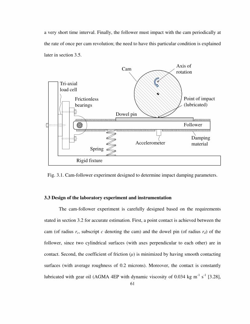
61

a very short time interval. Finally, the follower must impact with the cam periodically at

the rate of once per cam revolution; the need to have this particular condition is explained

later in section 3.5.

Fig. 3.1. Cam-follower experiment designed to determine impact damping parameters.

3.3 Design of the laboratory experiment and instrumentation

The cam-follower experiment is carefully designed based on the requirements

stated in section 3.2 for accurate estimation. First, a point contact is achieved between the

cam (of radius rc, subscript c denoting the cam) and the dowel pin (of radius rd) of the

follower, since two cylindrical surfaces (with axes perpendicular to each other) are in

contact. Second, the coefficient of friction (µ) is minimized by having smooth contacting

surfaces (with average roughness of 0.2 microns). Moreover, the contact is constantly

lubricated with gear oil (AGMA 4EP with dynamic viscosity of 0.034 kg m-1

s-1

[3.28],

Spring

Follower

Frictionless

bearings

Accelerometer

Rigid fixture

Dowel pin

Tri-axial

load cell

Point of impact

(lubricated)

Cam

Damping

material

Axis of

rotation

62

[3.29]), hence µ is taken to be as low as 0.2. Third, the flexural vibrations in the follower

(of width wb, subscript b denoting the bar) are minimized using a damping material (Sika

damp 620 [3.30]). Fourth, a tri-axial force transducer (PCB 260A01 [3.31]) located at the

follower hinge measures the reaction forces along ˆx

e (horizontal) and ˆye directions,

while the shock accelerometer (PCB 350B02 [3.32]) attached to the follower near the

contact point (at a distance of la from follower pivot) measures its tangential acceleration.

Both these transducers (capable of accurately recording the impacts) are simultaneously

sampled at a very high frequency of 204800 Hz using the LMS Scadas III [3.33] data

acquisition system. Finally, the contact is maintained when Ωc is low; however, the

follower (of length lb) starts losing contact and making impacts as Ωc is increased

considerably. As observed by Alzate et al. [3.8], the system quickly goes into a chaotic

state once Ωc is increased beyond a certain limit. Hence a variable speed electric motor is

used to carefully control Ωc, so that the system does a periodic impact of exactly once per

revolution of the cam. A digital tachometer (Neiko tools, USA) is used to accurately

measure Ωc. The variation in Ωc during the impacts is found to less than 2.5% of the

mean value, which is the same even when there is no load on the cam (follower is not in

contact with the cam).

3.4 Analytical model

3.4.1 Kinematics of the system

Fig. 3.2 shows a sketch of the analytical model with a contact mechanics

formulation for the experiment. The cylindrical cam rotates about E which is at a distance

e from the centroid (Gd). The linear stiffness of the coil spring supporting the bar is ks and

63

it is grounded at a distance dy below the bearing pivot P and at a distance of dx from it

along ˆx

e . The angle made by the follower with ˆx

e is given by α(t) measured in the

clockwise direction, while the angular displacement of the cam in the counter-clockwise

direction is given by Θ(t). The instantaneous points of contact in the cam and the follower

are given by Oc and Ob, respectively. A moving coordinate system ˆ ˆ( , )i j attached to the

follower is defined with its origin at Q where i is orthogonal to the follower. The vector

cQO

in the ˆ ˆ( , )i j coordinate system is given by ˆ ˆi ji jψ ψ+ as shown in Fig. 3.2. The 0-

state is defined with Θ0 and α

0 (with superscript 0 representing the 0-state), as discussed

by Sundar et al. [3.9] for a similar system. The contact mechanics is represented by point

contact stiffness (kλ) and impact damping (cλ) elements. The chief assumptions in the

analytical formulation are as follows: (1) The friction does not affect the impact

mechanism and it follows a Coulomb friction model; (2) The coil spring supporting the

follower is linear; and (3) The bending moment in the follower is negligible, while the

amplitude of flexural vibrations are negligibly small compared to the amplitude of

angular oscillations due to impact;

At the 0-state, α0 and Θ

0 is defined as the following,

( )

( )

4 2 2 2 2

0 1

2 2

0.5 2

0.5 2cos ,

b d cx x y x

b d cy

x y

PE PE PE PE w r r e

PE w r r e

PE PE

α −

+ − + + +

+ + + + = +

(3.3)

0 0 .2

π αΘ = − (3.4)

64

Fig. 3.2. Analytical contact mechanics model of the experiment shown in Fig. 3.1.

65

Here x

PE

and y

PE

are the magnitudes of PE

along ˆx

e and ˆye , respectively. Using

the procedure discussed by Sundar et al. [3.9], the moving coordinates (ψi(t) and ψj(t))

and their time derivates are calculated using the following equations:

( ) ( ) ( )( )( ) ( )

0 0 0

0

( ) sin ( ) 2 0.5 cos ( ) 1

[sin ( ) sin ( ) ( ) ],

i c d bt t r r w t

e t t t

ψ χ α α α α

α α

= − + + + − −

+ + Θ − + Θ (3.5)

( ) ( ) ( )

( ) ( )

0 0 0

0

( ) 1 cos ( ) 2 0.5 sin ( )

cos ( ) cos ( ) ( ) ,

j c d bt t r r w t

e t t t

ψ χ α α α α

α α

= − − + + + −

− + Θ − + Θ

(3.6)

( ) ( ) ( )

( ) ( )( )

0 0 0

0

( ) cos ( ) ( ) 2 0.5 sin ( ) ( )

cos ( ) ( ) cos ( ) ( ) ( ) ( ) ,

i c d bt t t r r w t t

e t t t t t t


α α α α

= − − + + −

+ + Θ − + Θ + Θ

ɺ ɺ ɺ

ɺɺ ɺ (3.7)

( ) ( ) ( )

( ) ( )( )

0 0 0

0

( ) sin ( ) ( ) 2 0.5 cos ( ) ( )

sin ( ) sin ( ) ( ) ( ) ( ) .

j c d bt t t r r w t t

e t t t t t


α α α α

= − + + + −

+ + Θ − + Θ + Θ

ɺ ɺ ɺ

ɺɺ ɺ (3.8)

Here, 0 ( ) ( )jt tχ χ ψ= + , where χ(t) is the moment of the Fλ(t) about P and is given by the

instantaneous magnitude of bPO

along j .

3.4.2 Non-contact regime

When the instantaneous value of ψi(t) > 0 the follower is not in contact with the

cam, the equation of motion depends only on the dynamics of the follower and coil

spring. It is given by the following, where P

bI is the moment of inertia of the follower

(along with the damping material) about P, mb is the mass of the follower (along with the

damping material), lb is the distance from the center of gravity of the follower (Gb) from

P:

66

( )( ) cos ( ) ( ) .P

b b g s xI t m gl t F t dα α= −ɺɺ (3.9)

Here, Fs(t) is the elastic force from the coil spring which is given as follows, where u

sL is

the undeflected length of the spring,

( ) ( )( ) tan ( ) 0.5 sec ( ) .u

s s s y x bF t k L d d t w tα α = − + + (3.10)

The eq. (3.9) is solved numerically for a given value of Ωc, as long as ψi(t) > 0. The

system goes to a contact regime once ψi(t) goes less than 0 and the response of the system

has to be calculated using the contact mechanics formulation, which is discussed next.

3.4.3 Contact regime

Using the contact mechanics formulation, the response of the system is calculated

using Hertzian contact theory [3.26]. The contact stiffness for a point contact is

calculated as,

( ) ( )0.54

( ) ( ) .3

e e

i ik t Y tλ ψ ρ ψ= (3.11)

Here, Y is the Young’s modulus (with superscript e denoting equivalent) given by the

following, where ν is the Poisson’s ratio,

12 21 1

.e c b

c b

YY Y

ν ν−

− −= +

(3.12)

The equivalent radius of curvature at the contact (ρe) is given by,

11 1( ) ( ) .e

c dr rρ

−− − = + (3.13)

The impact damping is defined as,

( )( ) ( ) .n

i ic t tλ ψ β ψ= (3.14)

67

The total contact force is given by,

( ) ( )( ) ( ) ( ) ( ) ( ).i i i iF t k t t c t tλ λ λψ ψ ψ ψ= − − ɺ (3.15)

Taking the moment balance of the forces acting on the follower about P, the equation of

motion in the contact regime is calculated as,

( ) ( )( ) cos ( ) ( ) ( ) ( ) ( ) 0.5 2 .P

b b g s x f b dI t m gl t F t d F t t F t w rλα α χ= − + − +ɺɺ (3.16)

Here, Ff(t) is the friction force given by

( )( ) ( ) sgn ( ) .f rF t F t v tλµ= (3.17)

Here, vr(t) is the relative sliding velocity at the contact point given by

( ) ( )( ) ( ) sin ( ) ( ) ( ) ( ) .r j cv t t r e t t t tψ α α= − + + Θ + Θ ɺɺ ɺ (3.18)

Note that from eq. (3.16), Ff(t) does not significantly affect the dynamics of the

system as its moment arm (0.5wb + 2rd) is very small compared to χ(t) and moreover µ is

very low. The system response is computed in the non-contact regime by solving eq.

(3.9), while in the contact regime by solving eq. (3.16). The system constantly switches

between these two regimes when Ωc is greater than a certain value, depending on the

system. At the very beginning of the simulation (0) *α α= and (0) 0α =ɺ are used as

initial conditions, where α* is the value of α(t) at the static equilibrium point (with

superscript *). This is evaluated using eqs. (3.5), (3.6) and (3.16) in the Jacobian matrix

method as discussed by Sundar et al. [3.9]. After this the initial conditions for each

regime is taken from the final state of the previous regime.

68

3.5 Estimation of the impact damping parameters (β and n)

3.5.1 Time-domain based technique to estimate the system response

The reaction forces along ˆx

e and ˆye (Nx and Ny, respectively, as shown in Fig.

3.2) and ( )tαɺɺ (calculated by dividing the measured tangential acceleration of the follower

by la) are the experimental data measured in the time-domain. The geometrical

parameters and inertia are obtained directly from the experiment. The entire procedure is

performed in the time-domain as impacts excite a wide range of frequencies (including

the natural frequencies of the cam-follower system and flexural vibrations of the

follower), and hence the frequency domain data cannot be used directly. Some of the

important numerical issues for which care needs to be taken in this estimation process are

as follows. First, the measured ( )tαɺɺ is numerically integrated obtain ( )tαɺ , which is

numerically integrated again to obtain the system response ( ( )tα ). The integration

process does not give the DC component of the signal, moreover numerical integration

process has inherent errors [3.34] (truncation and round-off) associated with it. Also since

integration has to be performed twice, these errors would have a cumulative effect on

α(t). Thus, higher accuracies can be achieved by having a shorter time resolution (τ) and a

smaller length of integration vector. Second, the magnitude of indentation (ψi(t)) during

contact is very small compared to the maximum value of α(t) in the non-contact regime

and the time of impact is very short. Hence it is very difficult to accurately estimate ψi(t)

during impacts from the experimental data.

The following technique is adopted to minimize the errors due to the numerical

integration and to estimate the DC component of α(t). The impact damping estimation

69

procedure discussed later in section 3.5.2 can be employed even without adopting this

technique, if α(t) can be accurately calculated from the experiment. The measured time-

domain data (forces and acceleration) have many impacts, but each impact is considered

an independent event for the purpose of analysis. Furthermore, each impact event is

divided into two sub-events, namely contact and non-contact. The contact sub-event

begins when the cam and the follower are just in contact (ti = 0, superscript i represents

experimental data for an impact event) with 0i

iψ = and ends when the follower looses

contact with the cam ( i i

at t= ). Then the non-contact sub-event starts and lasts until the

follower next comes into contact with the cam ( i i

et t= ). The experimental angular

acceleration for each impact event is measured as ( )i itαɺɺ and its time-average

( )( )i

i i

ttαɺɺ should be 0 since the impacts are periodic (as stated in section 3.3).

However, generally this is not the case as the measured data has some errors, and hence

( )i

i i

ttαɺɺ is subtracted from ( )i i

tαɺɺ . Then ( )i itαɺɺ is integrated numerically using the

Runge-Kutta method to get ( )i itαɺ . Though ( )

i

i i

ttαɺ should be 0, it is not due to the

errors of the numerical integration technique. This is eliminated by subtracting ( )i

i i

ttαɺ

from ( )i itαɺ . The resultant signal is again integrated numerically to get ( )i i

tα . The fact

that the follower impacts exactly once per revolution of the cam, is used again to

calculate the DC component of ( )i itα . For a given system, the time period of each

impact ( i

et ) depends on its state at the end of the contact sub-event. Writing it

70

mathematically as follows where Ξ is a function that gives the time required by the

follower to return to its initial position based on initial conditions,

( )( ), ( ) .i i i i i

e a at t tα α= Ξ ɺ (3.19)

Equation (3.9) is solved iteratively with known ( )i i

atαɺ and different values of α as initial

conditions to evaluate Ξ. The time required for the follower to come back to same initial

position is calculated for each α. The value of α for which the calculated time matches

with i

et , is chosen ( )i i

atα since 0i

at ≈ (due to extremely short time of contact sub-event).

The DC component of ( )i itα (calculated by numerical integration) is adjusted so that

( ) ( )i i

a

i i i i

at tt tα α

== . The angle of the cam at t

i = 0 ( )(0)iΘ is calculated from eq. (3.5) by

replacing α(t) with (0)iα , forcing ψi(t) = 0 and solving for Θ(t). Thus the time-history of

Θ can be calculated as,

( ) (0) .i i i i

ct tΘ = Θ + Ω (3.20)

3.5.2 Signal processing procedure to estimate β and n

It is not possible to have a direct method to estimate the impact damping

parameters, because of their inter-relationship with the measured acceleration and

reaction forces. Hence they are identified using an indirect method of comparing the

experimental data for each impact with the results from analytical model with trial values

of β and n which is defined as simulation S1 (where S1 represents simulation with trial

values). To aid in the comparison process, the ( )i iF tλ

during contact ( 0 i i

at t< < ) is

calculated from the measured data using the force balance as,

( ) ( )( ) ( ) ( ) sin ( ) ( ) ( ) cos ( ) .i i i i i i i i i i i i i

b g x y s bF t m l t N t t N t F t m g tλ α α α = + + + − ɺɺ (3.21)

71

Here ( )i

sF t is calculated from eq. (3.10) by replacing α(t) with ( )i itα . Also the maximum

amplitude of response ( )i

mα is calculated as the following where ‘max’ is a function that

returns the maximum value of a set of inputs,

( )max ( ) .i i i

m tα α= (3.22)

The results of simulation S1 are obtained for each impact event by solving the

equations of motion of the contact sub-event (eq.(3.16)) with (0)iα and (0)iαɺ as initial

conditions from the experimental data of the impact event, followed by the equation of

motion in the non-contact sub-event (eq. (3.9)) until 1S i

et t= (superscript S1 represents

results with simulation S1 with trial values of β and n for the corresponding impact event).

Simulation S1 is conducted using different trial values of β and n for each impact event to

compare with the experimental results. Similar to the experimental results 1 1( )S S

F tλ,

1 1( )S S

i tψ and 1S

mα are estimated for each simulation. The following residues are defined to

compare the experimental results with that of simulation S1:

1

1 ,

S i

m m

i

m

α α

α

−Λ =

( )

( )

12

0

2

2

0

( ) ( ) .

,

( ) .

ie

ie

t

Si

t

i

F t F t dt

F t dt

λ λ

λ

−

Λ =∫

∫

( ) ( )( )

1 1 1

3

( ). ( )..

( ).

S S Si i i

i i i i

i i i

i i

F d F d

F d

λ λ

λ

ψ ψ ψ ψ

ψ ψ

−Λ =

∫ ∫∫

(3.23 a - c)

72

The maximum response of the system after the impact is the criterion considered for the

first residue (Λ1). The second residue (Λ2) is based on the root mean square difference in

the contact forces from the experiment and the simulated data in time-domain, while the

third residue (Λ3) uses the area under the hysteresis loop. The appropriate numerical

values for β and n are identified based on the impact damping model which gives the

minimum value of the average of the residues of all impact events. The estimation

procedure can be based on either of the residues. Hence the accuracy of the estimation

process using these residues will be discussed in section 3.6.

3.6 Error and sensitivity analyses on the estimation procedure

3.6.1 Error analysis

Before employing the procedure discussed in section 3.5, the robustness (using

error analysis) and accuracy (using sensitivity) of the procedure have to be critically

studied. The robustness can be better understood by the error in the residues for an ideal

case, since an indirect method of comparison is being employed for the estimation

process. Simulation S2 (where S2 represents simulation with known values) is defined as

solving the analytical model for each impact event with given initial conditions using

known values of damping parameters ( 2Sβ and 2Sn , superscript S2 represents simulation

S2). The force and acceleration time-histories from simulation S2 are used instead of the

experimental data in the procedure discussed in section 3.5 and the residues are

calculated using the simulation S1 with the 1 2S Sβ β= and 1 2S Sn n= . Ideally all three

residues should be 0, but that is not the case due to the approximations in the estimation

procedure.

73

The following parameters for the cam-follower experiment are selected to have an

accurate estimation of impact parameters: mb = 0.257 kg, rc = 17.5 mm, Ib = 3300 kg-

mm2, lg = 173 mm, la = 63 mm, lb = 86 mm, wb = 12.7 mm, rd = 3.2 mm, ks = 3319 N/m,

u

sL = 53 mm, dx = 35 mm and dy = 58 mm. The relative positions of the pivot points of

the cam and the follower are given by ˆ ˆ89 mm 27 mmx y

PE e e= +

. The material properties

for a steel cam and a steel follower are Yc = Yb = 210 GPa and νc = νb = 0.3. Inverse

kinematic analysis discussed by Sundar et al. [3.9] is employed for the current system

with the given parameters to obtain the regions on impact on an e/rc vs. Ωc map as shown

in Fig. 3.3. Table 3.1 gives the average residue per impact, calculated using simulation S1

and S2 with 1 2 2.524.7 GNsmS Sβ β −= = and 1 2 1.5S S

n n= = for different values for e/rc and

Ωc in the impact regime (shown in Fig. 3.3). As observed, the residues for all cases are

very low, which shows that the estimation procedure is very robust for these examples.

Also, it can be inferred that as e/rc increases, Λ1 reduces and reaches a minimum at e/rc =

0.2 and starts increasing again. With the increase in e/rc the signal to noise ratio

increases; hence Λ1 reduces, but for very high values of e/rc the system operates close to

a chaotic state. The noise here might be from experimental measurements or from the

numerical error (in solving equations of motion). Similar trends are not observed in the

cases of Λ2 and Λ3. As observed, the values of Λ1 are the lowest, followed by Λ3, with Λ2

being the highest. Fig. 3.4 compares sample hysteresis loops of simulations S1 and S2, for

a case with e/rc = 0.2, where */i iF F Fλ λ λ= and */i i

i i iψ ψ ψ= . It is observed that for this

case, a point contact the maximum value of Fλ during impact is about 3 orders of

74

magnitude greater than *Fλ

while the maximum value of ψi during impact is only about 2

two orders of magnitude greater than *

iψ . Also even for an ideal case there is not a very

good match in the hysteresis loop for low values of indentation. The relative accuracies

of the residues in estimating the damping parameters should not be decided from the Λ

values in Table 3.1, but should be decided from the sensitivity of these residues to

variation in β and n. Hence it is analyzed next.

Fig. 3.3. Regimes of contact and impact for the system (with parameters given in section

3.6.1) via Ωc vs. e/rc. Key: , Operational points (with periodic impacts) selected for the

purpose of error analyses.

0 0.05 0.1 0.15 0.2 0.25 0.3 0.35 0.45

10

15

20

25

30

35

40

Impacting regime

Contact regime

e/rc

Ωc

[Hz]

75

e/rc Ωc (Hz) Average Λ1 Average Λ2 Average Λ3

0.05 23 0.0056 0.0849 0.0024

0.10 18 0.0361 0.1032 0.0033

0.15 17 4.75 x 10-7

0.0703 0.0041

0.20 16 0.78 x 10-7

0.0728 0.0039

0.25 15 1.65 x 10-7

0.0834 0.0043

Table 3.1 Comparison of average residues per impact (Λ1, Λ2 and Λ3) using two

simulations (S1 and S2) with 1 2 2.524.7GNsmS Sβ β −= = and 1 2 1.5

S Sn n= = .

76

Fig. 3.4. Comparison of hysteresis loops for single impacts during simulation S2 (

2 2.524.7GNsmSβ −= and 2 1.5S

n = ) and simulation S1 (1 2S Sβ β= and 1 2S S

n n= ) given

e/rc = 0.2 and Ωc = 16 Hz. Key: , Simulation S1; , Simulation S2.

3.6.2 Sensitivity analysis

Table 3.2a gives the values of normalized residues ( Λ ) for simulation S2 (

2 2.524.7 GNsmSβ −= and 2 1.5S

n = ) and simulation S1 with 1 2S Sn n= with different values

of 1Sβ in the close proximity of 2Sβ . The residues are normalized based on its value

when 1 2S Sβ β= . The sensitivity of the residues to a change in β can be understood from

this table. It can be easily inferred that 1Λ has a very high sensitivity even to a very small

change in the value of β, compared to that of 2Λ and

3Λ . Also ideally Λ should be

lowest for 1 2S Sβ β= , but that is not the case with 2Λ and

3Λ , which may lead to an

0 10 20 30 40 50 60 700

200

400

600

800

1000

i

iψ

77

incorrect estimation of β. A similar analysis is performed to study the sensitivity of

residues to a change in n and the result is shown Table 3.2b. Compared to the other two

residues 1Λ is more sensitive to changes in n. Also unlike

1Λ , the lowest value does not

occur at 1 2S Sn n= for

2Λ and 3Λ . Thus Λ1 is more accurate than other residues and hence

it will be used in the estimation of the impact damping model for the experimental

system. Note that the estimation procedure using Λ1 uses only the measured acceleration

and not the forces.

The reasons for the inaccuracies of Λ2 and Λ3 are as follows. The residue Λ2 is

inaccurate because it is based on the calculated Fλ during the impact which is for a very

short time period. Since Λ2 uses the integration of Fλ over time even a small error in the

estimation of Fλ is magnified in the residue calculation. The residue Λ3 is based on

hysteresis loop where Fλ is plotted against ψi which is very small in magnitude (< 50 µm)

during contact compared to the magnitude of ψi (~ 20 mm) during non-contact.

Moreover, ψi(t) is calculated using α(t) which has some error caused by numerical

integration. Hence, even a small error in the estimation of ψi results in a very high error in

the hysteresis loop. Thus, the sampling frequency should be much higher (than the one

which is used in this experiment) to use Λ2 and Λ3 in the estimation procedure.

78

Normalized

Residue

1 20.98S Sβ β= 1 20.99S Sβ β=

1 2S Sβ β=

(Ideal

case)

1 21.01S Sβ β= 1 21.02S Sβ β=

1Λ 1.17 x 10

5 0.582 x 10

5 1 0.574 x 10

5 1.14 x 10

5

2Λ 0.94 0.95 1 1.05 1.06

3Λ 0.95 0.96 1 1.05 1.06

a) For different values of 1Sβ in the proximity of 2Sβ with constant value of 1 2S Sn n= .

Normalized

Residue

1 20.98S Sn n= 1 20.99S S

n n=

1 2S Sn n=

(Ideal case)

1 21.01S Sn n= 1 21.02S S

n n=

1Λ 17.24 x 10

5 8.94 x 10

5 1 9.42 x 10

5 19.2 x 10

5

2Λ 2.49 1.67 1 0.76 1.16

3Λ 2.07 1.52 1 0.49 0.0086

b) For different values of 1Sn in the proximity of 2S

m with constant value of 1 2S Sβ β= .

Table 3.2 Comparison of normalized average residues per impact (1 2 3, andΛ Λ Λ ) using

simulation S2 (2 2.524.7GNsmSβ −= and 2 1.5

Sn = ) with e/rc = 0.2 and Ωc = 16 Hz.

79

3.7 Estimation of the impact damping from the measurements

The procedure discussed in section 3.5.2 had been employed to estimate the

impact damping parameters for the experimental system shown in Fig. 3.1. The

experiment was conducted for a given value of e/rc and the Ωc is slowly increased until a

one impact per revolution of the cam is achieved. The distinct impacts are visible in the

time histories of the normalized measured reaction forces ( *( ) ( ) /x xN t N t Fλ= ,

*( ) ( ) /y yN t N t Fλ= ) and measured acceleration shown in Fig. 3.5 from which T is

obtained and its relationship with 1/Ωc is verified. Fig. 3.6 shows normalized reaction

forces and acceleration data measured during the contact sub-event of a sample impact

from the experiment with e/rc = 0.13 and Ωc = 14.05 Hz (with measured T = 0.0712 s),

with all other parameters being the same as given in section 3.6.1, where the normalized

time is given by /i i i

at t t= . The values of the impact damping parameters identified

using minimization of Λ1 are β = 92.6 GNsm-2.55

and n = 1.55 (Note that the unit of β

depends on the numerical value of n, since n

i iβ ψ ψɺ should have the units of force).

The estimated value of n from the experimental data agrees closely with n = 1.5 which

would fit the contact force formulation of ( )1kF Fλ κδ= + ɺ , which is used by many

researchers [3.21, 3.23 - 25]. Hence the same procedure is followed by forcing n = 1.5

and β is evaluated as 49.3 GNsm-2.5

. Fig. 3.7 shows a comparison of the contact forces

of sample impact from the experimental data and the simulation S1 (with

1 -2.549.3 GNsmSβ = and 1 1.5S

n = ). As it can be inferred, though the damping

parameters have been selected based on the αm there is a good match in the shape and

80

peak value of the contact force. Also it is very important to note that for a very small

change in the value of n (about 3%) there is a very significant change in the estimated

value of β of about 46%. Hence n is more critical than β in the impact damping

formulation. Instead, if n is taken as 1.45, β is estimated as 29.3 GNsm-2.45

. The

experiment was repeated with different values of e/rc and Ωc and the same estimation

procedure had been followed to obtain β and n values.

81

Fig. 3.5. Time histories of the measured forces and acceleration with e/rc = 0.13 and Ωc

= 14 Hz (with other parameters given in section 3.6.1). a) Normalized reaction force

along ˆx

e ; b) Normalized reaction force along ˆy

e ; c) Angular acceleration of the follower.

0 0.5 1 1.5 2 2.5 3

-40

-30

-20

-10

0

10

20

30

40

50

a)

b)

c)

t [s]

0 0.5 1 1.5 2 2.5 3-30

-20

-10

0

10

20

30

0 0.5 1 1.5 2 2.5 3

-20

-10

0

10

20

30

40

[kra

d/s

2]

82

Fig. 3.6. Sample measured forces and acceleration during the contact sub-event from a

single impact from measurements shown in Fig. 3.5. a) Reaction forces; b) Angular

acceleration. Key: , Normalized reaction force along ˆxe ; , Normalized

reaction force along ˆy

e .

[kra

d/s

2]

0 0.2 0.4 0.6 0.8 1-10

0

10

20

30

40

50

a)

b)

it

0 0.2 0.4 0.6 0.8 1-20

-10

0

10

20

30

40

83

Fig. 3.7. Comparison of the contact forces (in the contact sub-event) from measured data

of Fig. 3.6 and simulation S1 (using the impact damping model selected based on

minimization of Λ1). Key: , Measured; , Simulation S1 (with

1 -2.549.3 GNsmSβ = and

1 1.5S

n = )

it

0 0.2 0.4 0.6 0.8 10

50

100

150

200

250

84

Since the estimated values of β and n were consistent, the repeatability of the experiment

and the accuracy of the estimation procedure are validated. Also, Sundar et al. [3.9]

estimated the values of κ for a similar system under dry conditions ranging from 3.25

s/m to 4.25 s/m which are comparable to κ = 3.8 s/m to 6.5 s/m (for n = 1.45 to 1.5,

respectively) for the current lubricated system.

To check if a viscous damping model can be used to represent an impact event, n

is forced to 0 and the same procedure is followed to obtain β = 1.47 kNs/m. A sample

hysteresis loop comparing the experimental data and simulation S1 (with 1 0S

n = and

1 1.47 kNs/mSβ = ) for the same is shown in Fig. 3.8. As it can be easily inferred there is

a very clear variation in the shape of the hysteresis loops. Furthermore, Fλ goes to a

negative value (tensile force) for part of the loop which is impractical, hence a viscous

damping model is not a good approximation to model impacts.

3.8 Equivalent coefficient of restitution

3.8.1 Governing equation

The equivalent ξ model is determined from the same measurements and it is used

to justify the impact damping parameters. Though researchers [3.9, 35] have assumed ξ =

constant, a more general model of the form is considered for the current analysis as given

by the following,

1a

vξ γ= − (3.24)

85

Fig. 3.8. Comparison of the hysteresis loops from measured data of Fig. 3.6 and

simulation S1 (using the viscous damping model selected based on minimization of Λ1).

Key: , Measured; , Simulation S1 with viscous damping ( 1 0S

n = and

1 1.47 kNs/mSβ = ).

Here, ξ decreases with the velocity of approach (va) at a constant rate of γ as suggested by

Hunt and Crossley [3.24]. Instead of using eq. (3.16) in the contact regime (for the

contact mechanics formulation), the state of the system after the impact (with superscript

a) is calculated for ξ formulation using the state of the system before impact (with

superscript b). From the definition of ξ,

0 5 10 15 20 25 30 35-50

0

50

100

150

200

250

300

i

iψ

86

a

i

b

i

ψξ

ψ= −ɺ

ɺ (3.25)

Since b

a iv ψ= ɺ , as per eq. (3.24),

1 b

iξ γ ψ= − ɺ (3.26)

From eqs. (3.25) and (3.26) the velocity of separation is calculated as

( )1a b b

i i iψ ψ γ ψ= − −ɺ ɺ ɺ . The state of the system before impact is obtained from the response

of the system in the non-contact regime when ψi(t) = 0. Rearranging the eq. (3.7) aαɺ is

calculated as

( )( ) ( ) ( )

( ) ( )

0 0 0

0

cos

cos 0.5 2 sin

cos cos

a a a

ia

a a

c b d

a a a

e

r w r

e

ψ αα

χ α α α α

α α

+ + Θ Θ=

− − + + −

+ + Θ − + Θ

ɺɺɺ (3.27)

Mathematically, in ξ formulation the system is in contact just for a single instant and

hence αa and Θ

a are approximated by their corresponding values before impact.

3.8.2 Estimation of the equivalent ξ model

Unlike the estimation of impact damping, a direct method can be employed to

estimate ξ. Since the state of the system just before impact (with superscript b) is needed

for this purpose, it is calculated using a numerical backward difference technique as

given by the following equations,

( ) (0) (0),b i i iα α τ α τα= − = − ɺ

( ) (0) (0),b i i iα α τ α τα= − = −ɺ ɺ ɺ ɺɺ

( ) (0) (0).b i i iτ τΘ = Θ − = Θ − Θɺ (3.28 a - c)

87

Velocity of approach ( b

iψɺ ) is calculated from eq. (3.7) by replacing ( )tα , ( )tαɺ and Θ(t)

with bα ,

bαɺ and bΘ , respectively, while the velocity of separation ( )a

iψɺ is the value of

( )i

i tψɺ when ( )itαɺ reaches maximum. Using eq. (3.25), ξ

i is estimated for each impact.

From ξi and ( )a

iψɺ , γ is identified using least square curve-fitting technique.

Analysis similar to the one discussed in section 3.6.1 has been performed to

evaluate the error in the estimation of ξ. Force and acceleration time histories from

simulation S3, which is an analytical model with known 3 0.8 s/mSγ = (other parameters

are same as given in section 3.6.1) is taken as reference. The ξi is estimated for each

impact for cases with different e/rc. The estimated γ and the % error associated with its

estimation is given in Table 3.3. It is inferred from the magnitude of errors that this

procedure yields very accurate γ for all the cases of e/rc. Fig. 3.9 shows the variation of ξi

with i

av on a normalized basis (on a scale of 0 to 1), for a sample case with e/rc = 0.1 and

Ωc = 18 Hz. The normalized ξi and i

av are calculated as follows, where ‘min’ is a function

that returns the minimum value of a set of inputs,

( ) ( )min( )

,max min

ii ξ ξ

ξξ ξ

−=

− (3.29)

( )( ) ( )

min.

max min

i

a ai

a

a a

v vv

v v

−=

− (3.30)

Fig. 3.9 also shows the ξ model estimated using the least square curve-fitting technique

with γ = 0.799 s/m.

88

For the same measured data (shown in Fig. 3.5), ξi is estimated for each impact

using the procedure (discussed in section 3.8.2) and the results are shown on a

normalized basis (using eqs. (3.29) and (3.30)) in Fig. 3.10. The least square curve-

fitting technique was applied to estimate γ as 0.758 s/m using data the measured data

and line of fit is also shown in Fig. 3.10. The average of the estimated ξ for all the

impacts is 0.75 with velocity of approach of 0.34 m/s which is similar to the value of ξ =

0.65 reported by Seifried et al. [3.35] for va of 0.3 m/s, under similar impacting

conditions.

e/rc Ωc (Hz)

Estimated γ

(s/m)

% error = 100r

r

γ γ

γ

−×

0.05 23 0.8 0

0.10 18 0.799 0.13

0.15 17 0.8 0

0.20 16 0.76 5.0

0.25 15 0.8 0

Table 3.3 Error in the estimation of ξ model using time histories from simulation S3

( )3 0.8s/mSγ = .

89

Fig. 3.9. Variation in estimated iξ (during different impacts) given b

iψɺ with e/rc = 0.10

and Ωc = 18 Hz. Key: , Simulation S3 (3 0.8s/m

Sγ = ) ; , Estimated ξ model

with γ = 0.799 s/m (using least square curve-fitting technique).

i

av

0 0.2 0.4 0.6 0.8 10

0.2

0.4

0.6

0.8

1

90

Fig. 3.10. Variation in estimated iξ (during different impacts) with b

iψɺ for the

experimental data of Fig. 3.5. Key: , Experimental data for different impact; ,

Estimated ξ model with γ = 0.758 s/m (using least square curve-fitting technique).

3.8.3 Justification of the estimated impact damping parameters

The relationship between coefficient of restitution and impact damping

formulations has been derived by Hunt and Crossley [3.24] for vibroimpacts. Using this

0 0.2 0.4 0.6 0.8 10

0.2

0.4

0.6

0.8

1

i

av

91

formula the equivalent β for the estimated γ (0.758 s/m) is obtained as 9.1 GNsm-2.5

,

which is comparable to the values estimated experimentally in section 3.7 (49.3 GNsm-2.5

for n = 1.5 and 29.3 GNsm-2.45

for n = 1.45). Some reasons for the difference between the

β values are: a) Hunt and Crossley [3.24] derived the relationship for vibroimpacts under

dry condition assuming pure metal to metal contact, but the experiments were under

lubricated condition; b) Even a small change in n value affects β significantly; and c) the

ξ concept has inherent drawback [3.9, 3.23] and hence the experimental estimation of γ

might have some inaccuracies. Taking these points into consideration, the estimated

values for impact damping parameters are justified on an order of magnitude basis.

3.9 Conclusion

The major contributions of this experimental study are as follows. First, a new

cam-follower experiment has been designed for periodic impacts, and instrumentation

and data acquisition parameters have been carefully chosen to accurately measure forces

and motion during impacts which takes place within a very short time interval. Second, a

novel time-domain based technique to estimate α(t) is developed, which minimizes the

effect of errors associated with the numerical integration. Also a new signal processing

procedure using only the measured acceleration has been developed to estimate impact

damping parameters. Third, a better understanding of the impact damping model is

obtained, and the following issues (stated in section 3.2) have been resolved: a) The

contact mechanics model given by eq. (3.1) is an acceptable formulation for impacting

systems; b) The residue using αm is more accurate than other residues (using hysteresis

loop and contact forces) for the purpose of damping parameter estimation; c) The impact

92

damping model is more sensitive to the damping index (n) than the damping coefficient

(β); d) The estimated value of n is successfully compared with those reported in the

literature, while the value of β is justified on an order of magnitude basis; and e) The

viscous damping model is not appropriate for impacting systems. Since the proposed

signal processing procedure (using Λ1) does not require force measurements, it could be

extended to other mechanical systems. The chief limitation of this study is the indirect

estimation of impact damping model; thus future work may be directed towards

development of a direct method, possibly for a line contact.

93


[3.1] R. Singh, H. Xie, R.J. Comparin, Analysis of automotive neutral gear rattle.

Journal of Sound and Vibration 131 (1989) 177–196.

[3.2] M.Y. Wang, R. Manoj, W. Zhao, Gear rattle modelling and analysis for

automotive manual transmissions. Proceedings of the Institution of Mechanical

Engineers, Part D: Journal of Automobile Engineering 215 (2001) 241–258.

[3.3] S. Theodossiades, S. Natsiavas, Periodic and chaotic dynamics of motor-driven

gear-pair systems with backlash. Chaos, Solitons & Fractals 12 (2001) 2427–

2440.

[3.4] T. Sakai, Y. Doi, K. Yamamoto, T. Ogasawara, M. Narita, Theoretical and

experimental analysis of rattling noise of automotive gearbox. Society of

Automotive Engineers (1981) SAE paper 810773.

[3.5] K. Karagiannis, F. Pfeiffer, Theoretical and experimental investigations of gear-

rattling. Nonlinear Dynamics 2 (1991) 367–387.

[3.6] F.Y. Chen, A survey of the state of the art of cam system dynamics. Mechanism and

Machine Theory 12 (1977) 201–224.




623.

94

[3.8] R. Alzate, M. di Bernardo, U. Montanaro, S. Santini, Experimental and numerical

verification of bifurcations and chaos in cam-follower impacting systems.

Nonlinear Dynamics. 50 (2007) 409–429.

[3.9] S. Sundar, J.T. Dreyer, R. Singh, Rotational sliding contact dynamics in a non-

linear cam-follower system as excited by a periodic motion. Journal of Sound

and Vibration 332 (2013) 4280–4295.

[3.10] S.H. Cho, S.T. Ahn, Y.h. Kim, A simple model to estimate the impact force

induced by piston slap. Journal of Sound and Vibration 255 (2002) 229–242.

[3.11] R. Wilson, J. N. Fawcett, Dynamics of the slider-crank mechanism with

clearance in the sliding bearing. Mechanism and Machine Theory 9 (1974) 61–

80.

[3.12] E.E. Ungar, D. Ross, Vibrations and noise due to piston-slap in reciprocating

machinery, Journal of Sound and Vibration. 2 (1965) 132–146.

[3.13] G.S. Whiston, Impacting under harmonic excitation. Journal of Sound and

Vibration 67 (1979) 179–186.

[3.14] R. Palej, J. Niziol, On a direct method of analyzing impacting mechanical

systems. Journal of Sound and Vibration 108 (1986) 191–198.

[3.15] R.J. Comparin, R. Singh, Non-linear frequency response characteristics of an

impact pair. Journal of Sound and Vibration 134 (1989) 259–290.

[3.16] C.N. Bapat, N. Popplewell, K. McLachlan, Stable periodic motions of an impact-

pair. Journal of Sound and Vibration 87 (1983) 19–40.

95

[3.17] C.K. Sung, W.S. Yu, Dynamics of a harmonically excited impact damper:

Bifurcations and chaotic motion. Journal of Sound and Vibration 158 (1992)

317–329.

[3.18] S. Chatterjee, A.K. Mallik, Bifurcations and chaos in autonomous self-excited

oscillators with impact damping. Journal of Sound and Vibration 191 (1996)

539–562.

[3.19] D.M. Egle, An investigation of an impact vibration absorber. Journal of

Engineering for Industry 89 (1967) 653–657.

[3.20] S.W. Shaw, P.J. Holmes, A periodically forced impact oscillator with large

dissipation, Journal of Applied Mechanics 50 (1983) 849–857.

[3.21] C. Padmanabhan, R. Singh, Dynamics of a piecewise non-linear system subject

to dual harmonic excitation using parametric continuation. Journal of Sound and

Vibration 184 (1995) 767–799.



[3.23] M.A. Veluswami, F.R.E. Crossley, G. Horvay, Multiple impacts of a ball

between two plates - part 2: mathematical modelling, Journal of Engineering for

Industry 97 (1975) 828–835.

[3.24] K.H. Hunt, F.R.E. Crossley, Coefficient of restitution interpreted as damping in

vibroimpact. Journal of Applied Mechanics 42 (1975) 440.

[3.25] R.C. Azar, F.R.E. Crossley, Digital simulation of impact phenomenon in spur

gear systems. Journal of Engineering for Industry 99 (1977) 792–798.

96



(3) (1972) 323–342.

[3.27] M.A. Veluswami, F.R.E. Crossley, Multiple impacts of a ball between two plates

- part 1: some experimental observations. Journal of Engineering for Industry 97

(1975) 820–827.

[3.28] http://www.tribology-abc.com/ (Accessed 15 Aug 2013)

[3.29] http://www.doolittleoil.com/faq/viscosity-sae-iso-or-agma (Accessed 15 Aug

2013).

[3.30] http://gbr.sika.com (Accessed 15 Aug 2013)

[3.31] M. Eriten, A.A. Polycarpou, L.A. Bergman, Development of a lap joint fretting

apparatus. Experimental Mechanics 51 (8) (2011) 1405–1419.

[3.32] PCB piezotronics Inc., sensors for acceleration, shock, vibration and acoustic

measurements: Product catalog (Model 350B02). (http://www.pcb.com;

Accessed 15 Aug 2013), Depew, NY, 2004.

[3.33] LMS instruments. LMS SCADAS III data acquisition front-end,

(http://www.lmsintl.com, Accessed 15 Aug 2013), Breda, The Netherlands,

2008.

[3.34] P.J. Davis, P. Rabinowitz, Methods of Numerical Integration, Courier Dover

Publications 2007.

97

[3.35] R. Seifried, W. Schiehlen, P. Eberhard, Numerical and experimental evaluation

of the coefficient of restitution for repeated impacts. International Journal of

Impact Engineering 32 (2005) 508–524.

98

CHAPTER 4

ESTIMATION OF COEFFICIENT OF FRICTION FOR A MECHANICAL

SYSTEM WITH COMBINED ROLLING-SLIDING CONTACT USING

VIBRATION MEASUREMENTS

4.1 Introduction

Friction plays a significant role in the dynamics of mechanical systems under

sliding contacts [4.1 - 4.7]. The friction force is often modeled using the Coulomb

formulation, though the analyst must judiciously select the value of the coefficient of

friction (µ). In many prior experimental studies, µ is found from a simple translational

sliding contact system as summarized by Persson [4.8]. For instance, Espinosa et al. [4.9]

used a modified Kolsky bar apparatus, while Hoskins et al. [4.10] used sliding block of

rocks to estimate the normal and friction forces. Furthermore, the translational sliding

experiments were employed by Worden et al. [4.11] to estimate the dependence of

friction forces on displacement and velocity, and then by Schwingshackl et al. [4.12] to

model the non-linear friction interface. Such experiments (specific to translational sliding

contact) cannot be directly employed for a system with combined rolling-sliding contact

to estimate µ, since the kinematics at the contact is different. Accordingly, several

investigators have conducted sliding contact experiments using a pin-disk apparatus

99

[4.13, 4.14], two rotating circular plates [4.15], and a radially loaded disk-roller system

[4.16, 4.17]. Also, Kang and Kim [4.18] determined the Coulomb friction in sight

stabilization equipment using torque and angular displacement characteristics, while

Povey and Paniagua [4.19] estimated the bearing friction for a turbomachinery

application. Further, Radzimovsky et al. [4.20] conducted experiments on gears to

determine the instantaneous µ over a mesh cycle. However, none of the previous

combined rolling-sliding contact experiments rely on vibration measurements. Hence

there is a need to develop a combined rolling-sliding contact experiment to determine µ

for a mechanical system with vibration measurements under certain conditions.

Some researchers have experimentally studied cam-follower mechanisms [4.21,

4.22] from the stability and bifurcation perspective under impacting conditions. In

contrast, a cam-follower mechanism with combined rolling-sliding contact (with no

impacts) is used to experimentally determine µ in this study. Since µ cannot be directly

measured from vibration experiments, an analogous contact mechanics model [4.23] is

developed to aid the process. The goal is to vary the surface roughness, slide-to-roll ratio,

lubrication film thickness, contact pressure and velocities at contact (sliding and

entrainment). The proposed system could then be utilized to simulate the contact

conditions seen in drum brakes and geared systems.


Fig. 4.1 shows the mechanical system with an elliptic cam (with semi-major and

minor axes as a and b, respectively). The cam is pivoted at E along its major axis with a

radial runout, e, from its centroid (Gc, with subscript c denoting cam). The angle made by

100

the end point of the major axis (A) with the horizontal axis ( ˆxe ) is Θ(t), which is an

excitation to the system (where t represents the time). The equation of the elliptic cam is

given by the following, where r is the radial distance from Gc to any point on the

circumference of the cam, and ∆ is the polar angle of that point,

( )( ) ( )

2 2.

sin cos

abr

a b

∆ =∆ + ∆

(4.1)

The cam is in a point contact (at Oc) with the follower (at Ob, with subscript b denoting

follower), which consists of a thin cylindrical dowel pin (of radius rd) attached to a bar

(of length lb) of square cross-section (of width wb). The center of gravity of the follower

lies at Gb at a distance of lg from the pivot point P (using roller bearings) which is at dy

distance about the ground. The follower is supported by a linear spring (ks) along the

vertical direction ( ˆye ), which is at a distance of dx from P as shown in Fig. 4.1. The

angular motion of the follower is given by α(t) in the clockwise direction from the ˆx

e

axis; it is also the only dynamic degree-of-freedom of the system. The contact mechanics

at O between the cam and the follower is represented by non-linear contact stiffness (kλ)

and viscous damping (cλ) elements. A coordinate system ˆ ˆ( , )i j attached to the follower is

defined with its origin at Q where i is orthogonal to the follower. The angle subtended by

c cGO

from xe is given by φ(t), which is used in the following equation to calculate the

∆O(t) for the contact point Oc as,

( )( ) mod ( ) ( ),2 .O t t tϕ π∆ = −Θ (4.2)

101

Here, “mod” is the modulus function defined as: mod( , ) .floor( / )x y x y x y= − , if y ≠ 0.

The vector cQO

is represented in the ˆ ˆ( , )i j coordinate system by ˆ ˆi ji jψ ψ+ . When the

instantaneous value of ψi(t) is negative, that would ensure that the cam and the follower

are in contact.

Fig. 4.1 Example case: A mechanical system with an elliptic cam and follower

supported by a lumped spring (ks).

102

The scope of the current study is restricted to an estimation of µ under a mixed

lubrication and elastohydrodynamic lubrication (EHL) regimes. The key assumptions in

the proposed system are as follows: (i) The bearings at the follower pivot are frictionless

and rigid; (ii) the surfaces of the cam and follower have no other irregularities with the

exception of random surface roughness; (iii) the sliding friction between cam and the

follower can be described by the Coulomb friction model; (iv) the contact force can be

represented by the Hertzian point contact model [4.23]; and (v) the bending moment of

the follower is negligible. The specific objectives of this study are: (1) Develop a contact

mechanics model for a mechanical system with a combined rolling-sliding contact to

design a suitable experiment and to predict the dynamic response; (2) Design a controlled

laboratory experiment for the cam-follower system to measure dynamic forces and

acceleration; and (3) Propose a signal processing technique to estimate µ using Fourier

amplitudes of measured forces and acceleration an empirical formula for µ will be

suggested and potential sources of errors will be identified.

4.3 Contact mechanics model

The 0-state of the system (represented by superscript 0) is defined as the state

when 0cQO =

and the major axis is parallel to the follower (0 0α = −Θ ). In the 0-state

Q0, Ob

0 and Oc

0 are coincident. From the geometry of the system, α and the magnitude of

bPO

along j (χ) are calculated in the 0-state as,

103

( ) ( )4 2 2 2 2

0 1

2 2

0.5 2 0.5 2

cos ,b d b d

x x y x y

x y

PE PE PE PE w r b PE w r b

PE PE

α −

+ − + + + + +

= +

(4.3)

0 0 0cos( ) sin( ) .x y

PE PE eχ α α= − −

(4.4)

Here, x

PE

and y

PE

represent the magnitudes of PE

along ˆx

e and ˆy

e , respectively.

The instantaneous values of the moving coordinates ψi(t) and ψj(t) are determined from

α(t), Θ(t) and the system geometry using the following vector equation,

.b b c cPE PO O O O E= + +

(4.5)

Employing the vector polygon procedure discussed by Sundar et al. [4.24], the equations

for ψi(t) and ψj(t) are obtained as,

( ) ( ) ( )( ) ( )( ) ( ) ( ) ( )

0 0 0( ) sin ( ) ( ) 0.5 2 cos ( )

( ) sin ( ) ( ) sin ( ) ( ) 0.5 2 ,

i o b d

o b d

t e t r t w r t

r t t t e t t w r

ψ χ α α α α

α ϕ α

= + − + ∆ + + −

+ ∆ + − + Θ − + (4.6)

( ) ( ) ( )( ) ( )( ) ( ) ( )

0 0 0 0( ) cos ( ) ( ) 0.5 2 sin ( )

( ) cos ( ) ( ) cos ( ) ( ) .

j o b d

o

t e t r t w r t

r t t t e t t

ψ χ χ α α α α

ϕ α α

= − + − + ∆ + + −

− ∆ + + + Θ(4.7)

Differentiating Eqs.

(4.6) and (4.7) with respect to time, ( )i

tψɺ and ( )j

tψɺ are obtained as

follows:

( ) ( ) ( )( ) ( )( ) ( )( ) ( ) ( )

( )( )

0 0 0( ) cos ( ) ( ) ( ) 0.5 2 sin ( ) ( )

( ) cos ( ) ( ) ( ) ( ) ( ) sin ( ) ( )

cos ( ) ( ) ( ) ( ) ,

i o b d

o o

t e t t r t w r t t

r t t t t t r t t t

e t t t t


α ϕ α ϕ α ϕ

α α

= + − − ∆ + + −

+ ∆ + + + ∆ +

− + Θ + Θ

ɺ ɺ ɺ

ɺ ɺ ɺ

ɺɺ

(4.8)

104

( ) ( ) ( )( ) ( )( ) ( )( ) ( ) ( )

( ) ( )

0 0 0( ) sin ( ) ( ) ( ) 0.5 2 cos ( ) ( )

( ) sin ( ) ( ) ( ) ( ) ( ) cos ( ) ( )

sin ( ) ( ) ( ) ( ) .

j o b d

o o

t e t t r t w r t t

r t t t t t r t t t

e t t t t


ϕ α ϕ α ϕ α

α α

= + − + ∆ + + −

+ ∆ + + − ∆ +

− + Θ + Θ

ɺ ɺ ɺ

ɺ ɺ ɺ

ɺɺ

(4.9)

Here,

( )( ) ( )

( )( ) ( )( )

2 2

1.52 2

0.5 sin 2 ( ) ( ) ( )( ) .

sin ( ) cos ( )

o

o

o o

ab b a t t tr t

a t b t

ϕ − ∆ − Θ ∆ = ∆ + ∆

ɺɺɺ (4.10)

The angle φ(t) corresponding to the contact point Oc is determined at every instant

for a given α(t) and Θ(t) by locating the point on the elliptic profile of the cam which is

tangential to the follower. Hence the slope of the follower, sb(t) = tan(-α(t)), should be

equal to the slope of cam at Oc ( ( )c

Os t ) which is calculated as follows,

( )

21

2( ) tan ( ) tan

tan ( ) ( )

c

O

bs t t

a t tϕ−

= Θ + −

− Θ (4.11)

Equating sb(t) and ( )c

Os t and rearranging, φ(t) is calculated by the following:

( )

21

2( ) ( ) tan

tan ( ) ( )

bt t

a t tϕ

α−

= Θ − − Θ

(4.12)

The equation of motion of the follower when it is in contact with the cam is

derived by balancing the moments (from Fig. 4.2) about P as,

( ) ( )( ) cos ( ) ( ) ( ) ( ) ( ) 0.5 2 .P

b b g s x n f b dI t m gl t F t d F t t F t w rα α χ= − + − +ɺɺ (4.13)

Here, P

bI is the moment of inertia of the follower about P, mb is the mass of the follower,

g is the acceleration due to gravity, and χ(t) is the moment arm of the contact force about

105

the pivot P. The elastic force from the spring, Fs(t), is given by the following, where u

sL

is the original length of the follower spring:

( ) ( )( ) tan ( ) 0.5 sec ( ) .u

s s s y x bF t k L d d t w tα α = − + + (4.14)

The normal force (Fn(t)) arising from the point contact with the cam is given by,

( )( ) ( ) ( ) ( ).n i i iF t k t t c tλ λψ ψ ψ= − − ɺ

(4.15)

The non-linear contact stiffness is defined for a point contact based on the Hertzian

contact theory [4.23] as,

( ) ( )0.54

( ) ( ) ( ) .3

e e

i ik t Y t tλ ψ ρ ψ=

(4.16)

Here, Y is the Young’s modulus (with superscript e denoting equivalent) in accordance

with the Hertzian contact theory given by the following, where ν is the Poisson’s ratio,

12 21 1

.e c b

c b

YY Y

ν ν−

− −= +

(4.17)

The equivalent radius of curvature at the contact (ρe(t)) and the radius of curvature of the

elliptical cam at Oc (ρc(∆o(t))) are given by,

( )( )1

1 1( ) ( ) ( ) ,e

c o dt t rρ ρ

−− − = ∆ +

(4.18)

( )( )( ) ( )( )

1.52 2

0

sin ( ) cos ( )

( ) .o o

c

a t b t

tab

γ γρ

∆ + ∆ ∆ = (4.19)

106

Fig. 4.2 Free-body diagram of the follower; refer to Fig. 4.1 for the two coordinate

systems.

The viscous contact damping is given by the following expression, where ζ is the modal

damping ratio which will be experimentally found under lubricated conditions, as

explained later in section 4.4,

( )2

2.

*

P

bIcλ

ζϑ

χ= (4.20)

Here, ϑ is the linearized natural frequency of the system, and χ* is value of χ(t) at the

static equilibrium point (discussed in later in this section). The friction force is given as,

107

( )( ) ( )sgn ( ) .f n r

F t F t v tµ= (4.21)

Here the relative sliding velocity, vr(t) is given by,

( ) ( ) ( ) ( )( ) ( ) ( ) sin ( ) ( ) sin ( ) ( ) ( ) ( ) .r j

v t t r t t t e t t t tψ ϕ α α α= − ∆ + + + Θ + Θ ɺɺ ɺ (4.22)

The static equilibrium point is used as the initial condition while numerically

solving Eq. (4.13). In Eqs. (4.6), (4.7) and (4.13), α(t), ψi(t), and ψj(t) are replaced with

their corresponding values at the static equilibrium point (with superscript *), and all

time-derivative terms are set to zero and solved. Using the method of Jacobian matrix as

discussed by Sundar et al. [4.24], ϑ is then calculated at the static equilibrium point.

4.4 Experiment for the determination of µ

Since the measured time domain signals are bound to have significant noise, a

frequency domain based signal processing technique is preferred for the estimation of µ.

Accordingly, measured forces and acceleration must not be affected by discontinuities

and system resonances. Design criteria for the experimental system can be given by the

following. First, the follower must always be in contact with the cam, as a loss in contact

would generate impulses in force and acceleration signals. Second, vr(t) should not

change direction during the operation, as that would induce a sudden change in the

direction of the Ff(t), thereby making the measured forces discontinuous. Furthermore,

the variation in vr(t) should be minimal. Third, the cam should rotate with a constant

speed (Ωc) in order to accurately measure the spectral contents of forces and acceleration.

Fourth, at least the first five harmonics of Ωc should lie in the stiffness controlled regime.

Fifth, the experiment should permit a mixed lubrication and EHL regimes. Finally, a

variation in the slide-to-roll ratio should be possible in the experiment.

108

Fig. 4.3 shows the schematic of a cam-follower experiment having a hollow

cylindrical cam of outer radius, a, driven by the output shaft of an electric motor. The

radial runout between the center of the rotation (axis of the shaft) and the centroid of the

cam can be easily varied. A point contact is obtained, as the cam and the dowel pin have

cylindrical surfaces with their axes oriented orthogonal to each other. The contact is

continuously lubricated using either a heavy gear oil (AGMA 4EP) [4.25, 4.26] or a light

hydraulic oil (ISO 32) [4.25, 4.26]. The follower is hinged at one of its ends with two

frictionless rolling element bearings and is supported by a coil spring. A tri-axial force

transducer (PCB 260A01 [4.27]) located at the follower hinge measures the reaction

forces, Nx(t) and Ny(t), along ˆxe and ˆ

ye , respectively. An accelerometer (PCB 356A15

[4.28, 4.29]) located at the end of the follower measures its tangential acceleration. These

are dynamic transducers with a very high frequency bandwidth [4.27, 4.29]. Both force

and acceleration signals are simultaneously sampled.

4.5 Identification of system parameters

4.5.1 Identification of geometrical parameters

The following parameters for the cam-follower system are carefully chosen to

satisfy the design constraints stated in section 4.4: mb=0.21 kg, a = b = 17.5 mm, Ib =

2020 kg-mm2, lg = 179 mm. lb = 89 mm, wb = 12.7 mm, rd = 3.2 mm, ks = 2954 N/m, u

sL

= 57 mm, dx = 40 mm and dy = 61 mm. The relative positions of the pivot points of the

cam and the follower are given by ˆ ˆ86mm 24mmx yPE e e= +

. The averaged surface

roughness (R) and root-mean-square roughness (Rrms) of the cam and follower surfaces

are measured using an optical profilometer. For the precision ground surfaces used in the

109

experiment Rc = 0.29 µm and Rb = 0.25 µm, while for sand-blasted surfaces Rc = 0.36 µm

and Rb = 0.89 µm. The key parameters that dictate a loss of contact between the follower

and the cam and the sign reversal in vr(t) are e and Ωc. Inverse kinematics [4.30] is

employed, as explained below, to predict a range of values for these two parameters over

which the system neither has a loss of contact nor a sign reversal in vr(t). For a given

value of e and Ωc, the angle of the follower (assuming it is just in contact) with the cam

(αk(t)) is kinematically calculated for different values of Θ(t) in the range [0, 2π]

(superscript k represents values calculated using the inverse kinematics). By setting ψi = 0

in Eq. (4.6), α

k(t) is calculated using the following equation,

( ) ( ) ( )( ) ( )( ) ( ) ( ) ( )

0 0 0sin ( ) ( ) 0.5 2 cos ( )

( ) sin ( ) ( ) sin ( ) ( ) 0.5 2 0.

k k

o b d

k k k k

o b d

e t r t w r t

r t t t e t t w r

χ α α α α

α ϕ α

+ − + ∆ + + −

+ ∆ + − + Θ − + = (4.23)

Here, rk(∆o(t)) is obtained using Eqs. (4.1) and (4.2) as,

( )( ) ( )

2 2( ) .

sin ( ) ( ) cos ( ) ( )

k

ok k k k

abr t

a t t b t tϕ α ϕ α

∆ = − + −

(4.24)

Equations (4.23) and (4.24) are solved along with Eq. (4.12) after replacing α(t) with

αk(t), to get r

k(∆o(t)), α

k(t) and φ

k(t). Then, differentiating α

k(t) with respect to t, ( )k

tαɺ

and ( )ktαɺɺ are obtained. The normal force is estimated (as stated below) from the

moment balance about P and by neglecting the moment due to Ff(t) in comparison with

the moment due to Fn(t) because of system geometry,

( )( ) ( ) ( )

( ) ( )

0 0 0

( ) ( ) cos ( )( ) .

cos ( ) 0.5 2 sin ( )

( ) cos ( ) ( )

P k k k

b s x b bk

n k k

b d

k k k

o

I t F t d m gl tF t

t b w r t

r t t t

α α

χ α α α α

α ϕ

+ −= − − + + − + ∆ −

ɺɺ (4.25)

110

Fig. 4.3 Mechanical system experiment used to determine the coefficient of friction (µ) at

the cam-follower interface.

Here, ( )k

sF t is calculated from Eq. (4.14) corresponding to αk(t). If the minimum value of

( )k

nF t calculated from Eq. (4.25) is negative, it would indicate that the follower would

lose contact with the cam during the steady-state operation. Similarly, the relative

velocity ( ( )k

rv t ) is kinematically calculated to check for any sign reversal from Eqs. (4.9)

and (4.22) by replacing α(t) and φ(t) with αk(t) and φ

k(t), respectively. The procedure

mentioned above is repeated for different values of e and Ωc to calculate the Ωc - e/a map

as shown in Fig. 4.4; the regimes with and without loss of contact and reversal in the

sliding velocity direction are clearly marked. All experiments are conducted in the e/a

Spring

Follower

Frictionless

bearings

Cam

Accelerometer

Rigid fixture

Dowel pin

Tri-axial

load cell

Output shaft of

the electric motor

Housing for electric motor

Lubricated

interface

111

range from 0.05 to 0.15, and Ωc is varied only between 10.1 Hz and 11.7 Hz; thus the

system is well within the contact regime (as shown) with a constant sgn(vr(t)) = -1 and

minimal variation in vr(t). With these parameters, the linearized natural frequency of the

system is found to be 1040 Hz for a steel cam and a steel follower (Yc = Yb = 200 GPa; νc

= νb = 0.3); thus the first five harmonics of Ωc lie in the stiffness controlled regime. Also,

the lubrication regime is identified based on the “lambda ratio” (Λ), which is the ratio of

minimum lubrication film thickness [4.31] to the composite surface roughness

( )( )0.52 2

, ,rms c rms bR R+ . With AGMA 4EP oil [4.25, 4.26] (with dynamic viscosity, η = 0.034

kg m-1

s-1

, pressure viscosity coefficient = 20x10-9

m2/N at 60° C) the system lies in the

EHL regime as Λ is approximately between 2 and 5. The system lies in the mixed

lubrication regime when ISO 32 oil [4.25, 4.26] (with η = 0.012 kg m-1

s-1

, pressure

viscosity coefficient = 18x10-9

m2/N at 60° C) is used, as lower values of Λ (0.7 to 1.5) is

utilized. Since the temperature at the contact is higher than the ambient (due to

continuous sliding), it is assumed that the interfacial oil operates at 60° C. Furthermore,

the slide-to-roll ratio which is given by the ratio of vr(t) (as given in Eq. (4.22)) and

entrainment velocity (ve(t) as defined below), varies between 0.75 and 1.25 for e/a =

0.116 and Ωc = 11.55 Hz as shown in Fig. 4.5. Here,

( ) ( ) ( ) ( )( ) ( ) ( ) sin ( ) ( ) sin ( ) ( ) ( ) ( ) .e j

v t t r t t t e t t t tψ ϕ α α α= + ∆ + + + Θ + Θ ɺɺ ɺ (4.26)

The slide-to-roll ratio ( )( ) ( )r e

v t v t could be easily changed by altering the geometry,

such as PE

, a, b and e.

112

Fig. 4.4 Classification of response regimes of the mechanical system with a circular cam

in terms of Ωc vs. e/a map with the parameters of section 4.5. Key: , Operational

range of the experiment.

0.1 0.2 0.3 0.4 0.5 0.6 0.7 0.8

10

15

20

25

30

e/a

Ωc

[Hz]

Loss of contact

regimeIn-contact

regime

No sign

reversal of vr(t)

Sign reversal

of vr(t)

113

Fig. 4.5 Slide-to-roll ratio for the cam-follower system with e/a = 0.12 and Ωc = 11.55 Hz

and other parameters of section 4.5.

4.5.2 Identification of the modal damping ratio

The modal damping ratio under lubrication depends on the oil viscosity and the

materials in contact; hence it is determined experimentally using the half-power

bandwidth method with both lubricants. The experimental setup consists of two masses

(m1 = 1.4 kg and m2 = 1.8 kg) connected by three identical point contacts which are

lubricated as shown in Fig. 4.6. These point contacts are obtained by placing three dowel

0 0.2 0.4 0.6 0.8 1

0.8

0.9

1

1.1

1.2

1.3

t [s]

Sli

de-

to-r

oll

rat

io

114

pins (rd = 3.2 mm) attached to m1 in one direction and two more dowel pins attached to

m2 in the orthogonal direction, as shown. The system is placed on a compliant base

(foam), and two accelerometers are attached to each mass. An impulse excitation is

imparted to the system in the vertical direction with an impact hammer. The response

accelerance spectrum of each mass along the vertical direction is then found by averaging

signals from two accelerometers. Impact tests are conducted with two lubricants. Fig. 4.7

shows the relative accelerance spectra (between m1 and m2), focusing on the system

resonance (~ 1000 Hz). As observed, there is a reduction in the amplitude and the natural

frequency with lubrication. For a single point contact, the damping ratio (ζ) with

unlubricated, ISO 32 oil and AGMA 4EP oil conditions are found to be 1.8%, 1.9% and

4.1%, respectively. Note that the damping for ISO 32 oil is very close to the dry case. It is

assumed that these values of ζ are also valid for the running cam-follower experiment.

4.6 Signal processing technique to estimate µ

The µ is estimated from measured reaction forces (Nx(t) and Ny(t)) along the ˆxe

and ˆy

e directions, respectively, and the tangential acceleration ( ( )b

l tαɺɺ ) of the follower at

its free end. By dividing the measured tangential acceleration by lb, ( )tαɺɺ is obtained, and

then numerically integrating it twice w.r.t. time, the time-varying component of α(t) is

computed, while the integration constant (αd) is obtained from the time-averaged value of

αk(t). The instantaneous elastic force Fs(t) is calculated from α(t) using Eq. (4.14). From

Fig. 4.2, Nx(t) and Ny(t) are evaluated as follows,

( ) ( ) ( )( ) ( )sin ( ) ( )cos ( ) ( )sin ( ) ,x n f b gN t F t t F t t m l t tα α α α= + − ɺɺ (4.27)

115

( ) ( )

( )

( ) ( )cos ( ) ( )sin ( )

( )cos ( ) ( ).

y n f

b b g s

N t F t t F t t

m g m l t t F t

α α

α α

= −

+ − −ɺɺ (4.28)

Fig. 4.6 Impulse experiment to determine the viscous damping ratio associated with the


arrangement showing the three point contacts. Key: , contact point.

Dowel pins

Impact hammera)

b)

Triaxial

accelerometer

Dowel pins

Rel

ativ

e ac

cele

ran

ce[m

/N-s

2]

Fig. 4.7 Relative accelerance spectra in the vicinit

, dry (unlubricated);

Rel

ativ

e ac

cele

ran

ce[m

/N-s

2]

850

1

5

10

15

Relative accelerance spectra in the vicinit

, dry (unlubricated);

900


, dry (unlubricated); , lubricated with AGMA 4EP oil;

Frequency [Hz]

900

116



32 oil.

Frequency [Hz]

950



Frequency [Hz]

1000

y of the system resonance. Key:

, lubricated with AGMA 4EP oil; , lubricated with ISO

1050


, lubricated with ISO

1050 1100


, lubricated with ISO

1100

117

Rearrange Eqs. (4.27) and (4.28) to yield the friction and normal forces as,

( ) ( )( ) ( )cos ( ) ( ) ( ) sin ( ) ,f x b y s

F t N t t m g N t F t tα α = + − − (4.29)

( ) ( )( ) ( ) ( )sin ( ) ( ) ( ) cos ( ) .n b g x y s b

F t m l t N t t N t F t m g tα α α = + + + − ɺɺ (4.30)

Since the dynamic force transducer used does not measure the DC component, a

technique to estimate µ is proposed that utilizes complex-valued Fourier amplitudes while

maintaining the phase relationship among the measured signals. First, the measured Nx(t),

Ny(t) and ( )tαɺɺ are converted to the frequency domain using the fast Fourier transform

(FFT) algorithm. Then, the harmonic reaction forces are reconstructed (with superscript

r) using only their DC components (with superscript d) and the fundamental harmonic

component of Ωc (with superscript 1) as,

( )1( ) cos ,r d

x x x cN t N N t= + Ω ( )1( ) cos .r d

y y y cN t N N t= + Ω (4.31 a, b)

In the above equation, 1

xN and

1

yN (where, ~ represents a complex-valued signal) are

known from measurements while d

xN and d

yN are unknown. Similarly, the following

harmonic signals have also been reconstructed as the following where, ( )( ) sin ( )s

t tς α=

and ( )( ) cos ( )c

t tς α= :

( )1( ) cos ,r d

s s s ct tς ς ς= + Ω

( )1( ) cos ,r d

c c c ct tς ς ς= + Ω

( )1( ) cos ,r d

n n n cF t F F t= + Ω ( )1( ) cos ,r d

f f f cF t F F t= + Ω

( )1( ) cos .r d

s s s cF t F F t= + Ω (4.32 a-e)

Since ( )tαɺɺ does not have a DC component, it is written as,

118

( )1( ) cos .r

ct tα α= Ωɺɺ ɺɺ (4.33)

Substituting these reconstructed harmonic signals in Eqs. (4.29) & (4.30) and

rearranging, the following DC components and first harmonic components of ( )r

fF t and

( )r

nF t are found as,

1 1 1 1 1 10.5 ,d d d d d d d d

f x c y s s s b s x c y s s sF N N F m g N N Fς ς ς ς ς ς ς= − + − + + − − (4.34)

1 1 1 1 1 1 1 1 ,d d d d d d

f x c y s x c y s b s s s s sF N N N N m g F Fς ς ς ς ς ς ς= − + − + − − (4.35)

1 1 1 1 1 1

0.5,

0.5

d d d d

b b s c b cd d d d d

n x s y c

x s y c s c

m l F m gF N N

N N F

α ς ςς ς

ς ς ς

+ −

= + + + + +

ɺɺ

(4.36)

1 1 1 1 1 1 1 1 10.5 .d d d d d d

n x s y c x s y c b c s c s c b bF N N N N m g F F m lς ς ς ς ς ς ς α= + + + − + + + ɺɺ (4.37)

From Eq. (4.21) and since sgn(vr(t)) = -1 is a constant, the following relationships can be

derived:

,d d

f nF Fµ= − (4.38)

1 1 .f n

F Fµ= (4.39)

Since ( )r

fF t and ( )r

fF t are exactly out-of-phase,

1 1.f nF F∠ = −∠ (4.40)

Substituting Eqs. (4.34) to (4.37) into Eqs. (4.38) to (4.40), three non-linear equations

with three unknowns (µ, d

xN andd

yN ) are obtained. These equations are numerically solved

119

to estimate µ. In order to computationally validate this technique, predicted forces and

acceleration from the contact mechanics model with e/a = 0.3, Ωc = 11.55 Hz and a

known µ = 0.3 are used. The signal processing technique (with 9460 Hz sampling

frequency and frequency resolution of 1.15 Hz) yields an estimate of µ as 0.302, which is

about 99.3% accurate. This method also accurately estimates d

xN andd

yN as -2.26 N and -

12.88 N, respectively, compared to the known values of -2.26 N and -12.7 N,

respectively.

4.7 Experimental results and friction model

Spectral tests are conducted under lubricated conditions with different surface

roughness levels at the contact. Care is taken during the experiments to record the steady

state force and acceleration measurements only after the initial transients have

sufficiently decayed. Using the measured data in the signal processing technique

discussed in section 4.6, the µ

(estimated value of µ) is indentified for various values of

mean surface roughness 0.5*( )m c b

R R R= + as shown in Fig. 4.8. This µ

is compared

with the values reported in the literature [4.13] for dry friction contact. A higher range is

observed in the case of a pure dry friction regime in comparison with µ

for the

lubricated contact. Also, observe that µ

with ISO 32 lubricant (with a low Λ value) is

similar to the dry friction contact case [4.13].

He et al. [4.32] used the Benedict-Kelly friction model [4.17] to develop an

empirical relationship between µ and Rm, but this was specific to a line contact in gears.

Hence that relationship is generalized for both point and line contacts as the following,

where < >t is the time-average operator,

120

1

2

2

log .( ) ( )m r et t

pC

C R v t v t

λµη

= −

(4.41)

Here, C1 and C2 are the arbitrary constants and pλ is the time-averaged Hertzian contact

pressure given by,

( )3

.2 ( ) ( )

n

e

i t

F tp

t tλ

π ρ ψ= (4.42)

With a non-linear curve-fitting technique, the constants of Eq. (4.41) are found from the

experimental results for each lubricant: C1 = 0.0288 µm and C2 = 2.03 µm for AGMA

4EP oil, and C1 = 0.0509 µm and C2 = 1.6512 µm for ISO 32 oil.

The measured force and acceleration spectra are compared with the contact

mechanics model (with estimated µ

) in Table 4.4 for a typical case with e/a = 0.116, Ωc

= 11.55 Hz and µ

= 0.51. The contact mechanics model successfully predicts the forces

and acceleration at the first three harmonics of Ωc, which are dominant compared with the

higher harmonics.

Fig.

the range) for the

32 oil;

Fig. 4.8 Estimated

the range) for the

32 oil; , dry contact

00

0.2

0.4

0.6

0.8

1

1.2

Estimated µ for different

the range) for the dry friction regime [13].

, dry contact - iron pin with steel disk

0.1

for different Rm

dry friction regime [13].

iron pin with steel disk

steel disk

0.2

121

m values and comparison with prior

dry friction regime [13]. Key:

iron pin with steel disk [2.13]

steel disk [2.13]

Rm

0.3

values and comparison with prior

Key: , With AGMA 4EP oil;

[2.13]; , dry contact

[2.13].

m [µm]

0.4

values and comparison with prior values (including

, With AGMA 4EP oil;

, dry contact -

0.5

values (including

, With AGMA 4EP oil; , With ISO

- copper pin with

0.6

values (including

With ISO

copper pin with

0.7

122

Harmonic of Ωc

αɺɺ (rad/s2)

Nx (N) Ny (N)

Measured Predicted Measured Predicted Measured Predicted

1 122.7 122.6 0.99 0.99 2.48 2.47

2 3.2 5.5 0.08 0.07 0.07 0.07

3 0.2 1.3 0.02 0.003 0.02 0.003

Table 4.4 Comparison of measurements and predictions (from the contact mechanics

model) with µ = 0.51 and e/a = 0.116 at the harmonics of Ωc = 11.55 Hz.

The normalized coefficient of friction ( µ ) for the empirical model of Eq. (4.41)

is defined as,

10 2

.

log( ) ( )

r et t

p

v t v t

λ

µµ

η

=

(4.43)

From Fig. 4.9 it is observed that µ monotonically increases with Rm. Also µ is lower

with AGMA 4EP (EHL regime) as compared to ISO 32 oil (mixed lubrication regime).

Fig. 4.9 compares some results of prior friction experiments [4.16, 4.33 - 35] in terms of

selected µ values which are calculated based on certain assumptions given a lack of

pertinent data. For instance, Shon et al. [4.16], Xu & Kahraman [4.33] and Furey [4.35]

conducted experiments under EHL regime, and hence their µ values are very low.

Conversely, Grunberg and Campbell [4.34] conducted experiments under poorly

lubricated conditions (mixed lubrication regime). It can be easily inferred that µ

123

decreases as Λ increases. There are some differences in the µ values from (Eq. (4.41))

and the ones reported in the literature; these may be attributed to different lubrication

regimes as well as potential sources of error in the µ estimation process which is

discussed next.

4.8 Potential sources of error in the estimation of µ

Some of the common measurement errors which are difficult to minimize include

the following. First, a variation in the frictional load torque on the cam causes small

variations in Ωc during the experiment. This in turn introduces inaccuracy in the

harmonic contents of the measured forces and acceleration, thereby affecting the

estimated µ. Second, a small error in the angular alignment (κ) of a force transducer could

measure Ny(t) cos(κ) instead of the actual Ny(t). From the static analysis it is found that

for κ = 5°, the µ estimate has only a 0.5 % error. Third, if the follower spring is oriented

at an angle of σ (from the vertical in the clockwise direction), the elastic force Fs(t) will

be as follows as opposed to the one given by Eq. (4.14),

( )( )

( ) ( )cos ( )

( ) tan ( ) 0.5 sec ( ) .cos ( )

s u

s s y x b

k tF t L d d t w t

t

αα α

α σ = − + + −

(4.44)

124

Fig. 4.9 Comparison of the modified Benedict-Kelley model from the results of Fig. 4.8

with friction values reported in the literature [4.16, 4.33 - 35]. Key: , Model for

AGMA 4EP oil (EHL regime) ; , Model for ISO 32 oil (mixed lubrication

regime), , Shon et al. [4.16]; , Xu and Kahraman [4.33]; , Grunberg and

Campbell [4.34]; , Furey [4.35].

Rm [µm]

µ

0 0.1 0.2 0.3 0.4 0.5 0.6 0.70

0.01

0.02

0.03

0.04

0.05

0.06

125

Also the reaction forces will have to be calculated from the following instead of using the

expressions of Eqs. (4.27) and (4.28),

( ) ( )

( ) ( )

( ) ( )sin ( ) ( )cos ( )

0.5 ( )sin ( ) ( )sin ,

x n f

b b s

N t F t t F t t

m l t t F t

α α

α α σ

= +

− −ɺɺ (4.45)

( ) ( )

( ) ( )

( ) ( )cos ( ) ( )sin ( )

0.5 ( )cos ( ) ( )cos .

y n f b

b b s

N t F t t F t t m g

m l t t F t

α α

α α σ

= − +

− −ɺɺ (4.46)

Based on the static force balance, the error in the estimation of µ is about 9% with only σ

= 1°, which is very significant.

The estimation of µ involves some error-prone numerical methods [4.36]. For

instance, bias errors [4.37] might be caused in the computation of the spectral contents of

forces and acceleration due to a coarse frequency resolution (constrained by the length of

the measured time domain signal) and the usage of Hanning window. Furthermore,

equations (4.38) to (4.40) are solved using the Levenberg-Marquardt algorithm which has

limited accuracy as dictated by its relative and absolute tolerance values [4.38].

The error in µ is simulated for the system with a circular cam for different values

of e under a constant Ωc = 11.55 Hz. Using the predicted force and acceleration responses

from the contact mechanics model (with known µ = 0.3) in signal processing technique,

µ

is calculated and the results are given in Table 4.5. For a very low value of e/a, the

error in µ

is high because the amplitude of αɺɺ (and the reaction forces) at the first

harmonic of Ωc is very small. As the amplitude of αɺɺ at the fundamental harmonic of Ωc

increases, the error reduces and reaches a minimum at e/a = 0.3 (error = 0.67%). Beyond

e/a = 0.3, the error again starts increasing since the amplitude of αɺɺ at the second

126

harmonic of Ωc becomes significant compared with that of the first. Next the error is

calculated for different Ωc with a constant e. The error monotonically decreases (as

observed from Table 4.6) with an increase in Ωc; this is because the amplitude of αɺɺ (and

the reaction forces) at the first harmonic of Ωc increases, while the amplitude ratio of the

second harmonic to the fundamental harmonic is a constant.

A similar analysis is done for the system with an elliptic cam given e/a = 0.1, for

different values of eccentricity ( )0.5

2

21 ba

∈= −

with known µ = 0.3 (other parameters

remaining the same as in section 4.5). Fig. 4.10 gives a map of Ωc - b/a, showing

different regimes that are obtained using the inverse kinematics procedure of section 4.5.

Comparison of Fig. 4.10 with Fig. 4.6 suggests that ϵ for an elliptic cam provides a

similar motion input as e does for a circular cam. Care is taken so that the system lies in

the regime without a loss of contact and no direction reversal of the vr(t). Table 4.7 shows

the µ

values for an elliptic cam for different ϵ at Ωc = 8.33 Hz. Only a small variation in

the error is observed. However, an increase in the ϵ increases the acceleration amplitude

at the second harmonic of Ωc due to a change in the type of motion input to the system.

Overall, it is inferred that µ can be satisfactorily estimated even for a system with an

elliptic cam.

127

Table 4.5 Error in the estimation of µ for the mechanical system with a circular cam for

different values of e at Ωc = 11.55 Hz.

e/a

αɺɺ (rad/s2) Estimated

µ

% error = –

100

known

known

µ µ

µ×

At the first

harmonic of Ωc

At the second

harmonic of Ωc

0.05 52.5 1.01 0.284 5.3

0.10 105.0 4.02 0.286 4.7

0.15 157.5 9.05 0.288 4.0

0.20 210.0 16.1 0.292 2.8

0.25 262.5 25.1 0.296 1.3

0.3 315.1 36.2 0.302 0.7

0.35 367.6 49.3 0.31 3.1

0.4 420.1 64.4 0.32 6.0

0.45 472.7 81.5 0.33 9.4

128

Table 4.6 Error in the estimation of µ for the mechanical system with circular cam for

different cam speeds with e/a = 0.1.

Ωc

[Hz]

αɺɺ [rad/s2] Estimated

µ

% error =

– 100

known

known

µ µ

µ×

At the first

harmonic of Ωc

At the second

harmonic of Ωc

2 3.24 0.135 0.28 6.7

5 20.26 0.84 0.281 6.3

8 51.77 2.15 0.283 5.7

11 97.9 4.1 0.285 5.0

14 158.5 6.6 0.288 4.0

17 233.8 9.7 0.292 2.7

21 356.7 14.9 0.297 1.0

129

Fig. 4.10 Classification of response regimes of a mechanical system with an elliptic cam

in terms of a Ωc – b/a map with e = 0.1a and other parameter values given in section 4.5.

Key: , Operational range of the simulation.

0 0.2 0.4 0.6 0.8 1

8

10

12

14

16

18

20

22

24

ϵ

Ωc

[Hz]

Loss of contact

regime

In-contact

regimeNo sign

reversal of vr(t)

Sign reversal

of vr(t)

130

Table 4.7 Error in the estimation of µ for the mechanical system with an elliptic cam at

Ωc = 8.33 Hz and e = 0.1 a.

4.9 Conclusion

The major contributions of these analytical and experimental studies are as

follows. First, a new vibration experiment has been designed to estimate µ for a

mechanical system with combined rolling-sliding contact under lubrication. This

experiment permits the contact pressure, “lambda ratio”, contact velocity (sliding and

entrainment), lubrication regime and surface roughness to be changed while satisfying the

design constraints. Thus, the same experiment can be used to estimate µ for similar

ϵ

αɺɺ (rad/s2) Estimated

µ

% error =

– 100

known

known

µ µ

µ×

At the first

harmonic of Ωc

At the second

harmonic of Ωc

0 52.2 2.18 0.283 5.7

0.31 52.1 52.7 0.281 6.2

0.44 52.1 104.9 0.281 6.2

0.53 52.05 156.8 0.284 5.5

0.6 52.0 208.4 0.288 4.2

0.66 51.95 259.7 0.294 2.2

131

combined rolling-sliding contact systems such as gears and drum brakes. Second, an

improved contact mechanics model for a mechanical system with an elliptic cam and

follower is formulated that successfully predicts the system responses, as theory and

experiment match well. This mathematical model yields a better understanding of the

system dynamics as well as the accuracy of the µ estimation procedure. Third, an

improved signal processing method is proposed to calculate µ using the complex-valued

Fourier amplitudes of measured forces and acceleration. The DC components of the

measured signals are also estimated by this method (along with µ) by numerically solving

a set of nonlinear equations. The chief limitation of this study is related to the angular

alignment of the follower spring. Also the error in µ

is controlled by the choice of

system geometry and cam speed; in particular the speed should be fairly low in order to

avoid impacting conditions.

132


[4.1] C.A. Brockley, R. Cameron, A.F. Potter, Friction-induced vibration, Journal of

Tribology 89 (2) (1967) 101–107.

[4.2] A.H. Dweib, A.F. D’Souza, Self-excited vibrations induced by dry friction, part 1:


[4.3] A.F. D’Souza, A.H. Dweib, Self-excited vibrations induced by dry friction, part 2:

Stability and limit-cycle analysis, Journal of Sound and Vibration 137 (2) (1990)

177–190.

[4.4] J. Kang, C.M. Krousgrill, The onset of friction-induced vibration and spragging,

Journal of Sound and Vibration 329 (17) (2010) 3537–3549.

[4.5] R.I. Leine, D.H. van Campen, A. de Kraker, L. van den Steen, Stick-Slip

vibrations induced by alternate friction models, Nonlinear Dynamics 16 (1)

(1998) 41–54.

[4.6] H. Ouyang, J.E. Mottershead, M.P. Cartmell, D.J. Brookfield, Friction-induced

vibration of an elastic slider on a vibrating disc, International Journal of

Mechanical Sciences 41 (3) (1999) 325–336.

[4.7] G. Sheng, Friction-induced vibrations and sound: Principles and applications,

CRC Press/Taylor & Francis Group, Boca Raton, 2008.

[4.8] B.N.J. Persson, Sliding friction, Surface Science Reports 33 (3) (1999) 83–119.

[4.9] H.D. Espinosa, A. Patanella, M. Fischer, A novel dynamic friction experiment

using a modified kolsky bar apparatus, Experimental Mechanics 40 (2) (2000)

138–153.

133

[4.10] E.R. Hoskins, J.C. Jaeger, K.J. Rosengren, A medium-scale direct friction

experiment, International Journal of Rock Mechanics and Mining Sciences 5 (2)

(1968) 143–152.

[4.11] K. Worden, C.X. Wong, U. Parlitz, A. Hornstein, D. Engster, T. Tjahjowidodo, F.

Al-Bender, D.D. Rizos, S.D. Fassois, Identification of pre-sliding and sliding

friction dynamics: Grey box and black-box models, Mechanical Systems and

Signal Processing 21 (1) (2007) 514–534.

[4.12] C.W. Schwingshackl, E.P. Petrov, D.J. Ewins, Measured and estimated friction

interface parameters in a nonlinear dynamic analysis, Mechanical Systems and

Signal Processing 28 (2012) 574–584.

[4.13] S.C. Lim, M.F. Ashby, J.H. Brunton, The effects of sliding conditions on the dry

friction of metals, Acta Metallurgica 37 (3) (1989) 767–772.

[4.14] M. Wakuda, Y. Yamauchi, S. Kanzaki, Y. Yasuda, Effect of surface texturing on

friction reduction between ceramic and steel materials under lubricated sliding

contact, Wear 254 (3 - 4) (2003) 356–363.

[4.15] S. Mentzelopoulou, B. Friedland, Experimental evaluation of friction estimation

and compensation techniques, Proceedings of the American Control Conference,

Baltimore, MD, USA, June 29 – July 1, 1994, 3132-3136.

[4.16] S. Shon, A. Kahraman, K. LaBerge, B. Dykas, D. Stringer, Influence of surface

roughness on traction and scuffing performance of lubricated contacts for

aerospace and automotive gearing, Proceedings of the ASME/STLE International

134

Joint Tribology Conference, Denver, USA. Oct 7 - 10, 2012, Paper # IJTC2012-

61212.

[4.17] G.H. Benedict, B.W. Kelley, Instantaneous coefficients of gear tooth friction,

ASLE Transactions 4 (1) (1961) 59–70.

[4.18] Y.S. Kang, K.J. Kim, Friction identification in sight stabilization system at low

velocities, Mechanical Systems and Signal Processing 11 (3) (1997) 491–505.

[4.19] T. Povey, G. Paniagua, Method to improve precision of rotating inertia and

friction measurements in turbomachinery applications, Mechanical Systems and

Signal Processing 30 (2012) 323–329.

[4.20] E.I. Radzimovsky, A. Mirarefi, W.E. Broom, Instantaneous efficiency and

coefficient of friction of an involute gear drive, Journal of Manufacturing Science

and Engineering 95 (1973) 1131–1138.



follower system, SIAM Journal on Applied Dynamical Systems 8 (2) (2009) 592–

623.


verification of bifurcations and chaos in cam-follower impacting systems,

Nonlinear Dynamics 50 (3) (2007) 409–429.


contact to random roughness of their surfaces, Journal of Sound and Vibration 22

(3) (1972) 323–342.

135

[4.24] S. Sundar, J.T. Dreyer, R. Singh, Rotational sliding contact dynamics in a non-

linear cam-follower system as excited by a periodic motion, Journal of Sound and

Vibration 332 (18) (2013) 4280–4295.

[4.25] http://www.tribology-abc.com/ (Accessed 25 May 2013)

[4.26] http://www.doolittleoil.com/faq/viscosity-sae-iso-or-agma (Accessed 25 May

2013)

[4.27] M. Eriten, A.A. Polycarpou, L.A. Bergman, Development of a lap joint fretting

apparatus, Experimental Mechanics 51 (8) (2011) 1405–1419.

[4.28] A. Gunduz, J.T. Dreyer, R. Singh, Effect of bearing preloads on the modal

characteristics of a shaft-bearing assembly: Experiments on double row angular

contact ball bearings, Mechanical Systems and Signal Processing 31 (2012) 176–

195.

[4.29] PCB Piezotronics Inc., ceramic shear ICP® accelerometer (Model 356A15):

Installation and operating manual (http://www.pcb.com; Accessed 25 May 2013).

[4.30] F. Y. Chen, Mechanics and Design of Cam Mechanism, Pergamon Press, 1982.

[4.31] H. S. Cheng, A Numerical Solution of the Elastohydrodynamic Film Thickness in

an Elliptical Contact, Journal of Lubrication Technology 92 (1970) 155–161.

[4.32] S. He, S. Cho, R. Singh, Prediction of dynamic friction forces in spur gears using

alternate sliding friction formulations, Journal of Sound and Vibration 309 (3-5)

(2008) 843–851.

136

[4.33] H. Xu, A. Kahraman, N.E. Anderson, D.G. Maddock, Prediction of mechanical

efficiency of parallel-axis gear pairs, Journal of Mechanical Design 129 (1)

(2007) 58.

[4.34] L. Grunberg, R. B. Campbell, Metal transfer in boundary lubrication and the

effect of sliding velocity and surface roughness, Proceedings of the Conference on

Lubrication and Wear, Institution of Mechanical Engineers, London, 1957, 297-

301.

[4.35] M. J. Furey, Surface roughness effects on metallic contact and friction, ASLE

Transactions 6 (1) (1963) 49–59.

[4.36] J. Stoer, R. Bulirsch, R. Bartels, W. Gautschi, C. Witzgall, Introduction to

Numerical Analysis, Springer, New York, 1993.

[4.37] H. Herlufsen, S. Gade, Errors involved in computing impulse response functions

via frequency response functions, Mechanical Systems and Signal Processing 6

(3) (1992) 193–206.

[4.38] D. W. Marquardt, An algorithm for least-squares estimation of nonlinear

parameters, Journal of the Society of Industrial and Applied Mathematics 11 (2)

(1963) 431–441.

137

CHAPTER 5

CONCLUSION

5.1 Summary

This study examines the non-linear dynamics and contact mechanics of system

with combined rolling-sliding contact using a cam-follower mechanism. The contact

dynamics especially coefficient of friction and impact damping are estimated using

analytical, experimental and numerical methods.

In chapter 2, the non-linearities of the cam-follower system have been

analyzed in this study. A contact mechanics formulation for a cam-follower system with

combined rolling-sliding contact has been developed, and the predictions with combined

viscous-impact damping models are successfully compared with the experimental results

reported by Alzate et al. [5.1]. The inaccuracy of the coefficient of restitution (ξ) concept

is analyzed using the approximate energy balance technique. The effect of friction non-

linearity on the dynamic forces is studied using discontinuous and smoothened dry

friction models. Finally, a linearized system is found to be inadequate in representing the

system with only kinematic non-linearity.

In chapter 3, the parameters of impact damping model for a point contact under

lubricated condition are estimated from time-domain measurements. An experiment is

138

designed and instrumented to measure force and acceleration in a system during periodic

impacts. A new time-domain based technique is developed to accurately calculate the

system response. An indirect signal processing estimation procedure (using residue

minimization) is developed to get the damping parameters using an analogous contact

mechanics model. Three different residues were defined and their accuracies were

analyzed. The estimated values of damping parameters were justified using literature

[5.2] and equivalent ξ model.

In chapter 4, a new experimental method to estimate the coefficient of friction (µ)

under lubricated condition for a system with combined rolling-sliding contact is

developed. The cam-follower experiment is designed to have continuous contact. A

contact mechanics model with an elliptic cam is developed from which the experimental

parameters satisfying the design constraints are obtained. A new signal processing

technique had been developed to estimate µ from the Fourier amplitudes of the measured

forces and acceleration. This technique has a very good numerical accuracy, as inferred

from the error analysis conducted. An empirical relation to get µ is derived based on

Benedict-Kelley model [5.3]. The different types of errors in the estimation process are

analyzed and it is found that, even a minor misalignment in the angle of the follower

spring causes large error in µ estimation.

5.2 Contributions

In this dissertation, several contributions emerge that are related to the

improved understanding of the non-linear contact dynamics of systems with combined

rolling-sliding contact. Some of the major contributions are as follows. First, the impact

139

damping model is estimated using the measurements of periodic impact events with point

contact, with the help of a new signal processing procedure (minimizing the inherent

errors associated with the numerical integration). Also some of the major issues regarding

impact damping model (stated in section 3.2) have been resolved. Furthermore, the

applicability of ( )1k

F κδ+ ɺ formulation and the inaccuracy of viscous damping for an

impacting system have been experimentally verified.

Second, the coefficient of friction has been determined for the cam-follower

system with combined rolling-sliding contact from the measured forces and acceleration

(without the DC component) using a new frequency-domain based technique. A

generalized model to predict µ for a given surface roughness under lubricated condition

(with point contact) is proposed. Also the major sources of error in the estimation process

have been quantified. Some of the other contributions from this research are the

following. This research yields better understanding of the inaccuracies of coefficient of

restitution formulation during impacts and the roles of the friction and kinematic non-

linearities in the sliding contact regime.

5.3 Future work

There are several paths to further extend the examination of the non-linear

dynamics and contact mechanics of systems with combined rolling-sliding contact. Each

path should be independent and build upon the knowledge gained from this research:

1. Improve the analytical model by developing a higher degrees-of-freedom

(DOF) system for a cam-follower system by relaxing the rigid pivot

140

assumption. The improved model will more accurately represent the real

system under higher loads.

2. Analyze the non-linear dynamics of system with different scenarios of cam

motion like, constant acceleration, constant deceleration, oscillating speeds

and friction torque dependent speed variation.

3. Seek semi-analytical solutions to the non-linear differential equations of motion

to achieve improved accuracy in the prediction of system response.

4. Perform similar experimental study with line contacts to widen the knowledge

of the contact mechanics of such system. A very high degree of precision is

required to obtain a line contact experimentally.

5. Develop a direct method to obtain the impact damping parameters with higher

accuracy, instead of using indirect method discussed in this research.

6. Examine the non-linear dynamics of cam-follower system with two

kinematically liked followers in contact with the cam. A 3 DOF system can be

developed for this purpose with a rotational DOF each for the followers and

the cam. Friction induced vibrations like stick-slip and sprag-slip can be

experimentally analyzed using this system, which is a simplified model of a

drum brake.

141



verification of bifurcations and chaos in cam-follower impacting systems.

Nonlinear Dynamics. 50 (2007) 409–429.

[5.2] K.H. Hunt, F.R.E. Crossley, Coefficient of restitution interpreted as damping in


[5.3] G.H. Benedict, B.W. Kelley, Instantaneous coefficients of gear tooth friction, ASLE

Transactions 4 (1) (1961) 59–70.

142

BIBLIOGRAPHY

R. Alzate, M. di Bernardo, G. Giordano, G. Rea, S. Santini, Experimental and numerical

investigation of coexistence, novel bifurcations, and chaos in a cam-follower system.

SIAM Journal on Applied Dynamical Systems 8 (2009) 592–623.

R. Alzate, M. di Bernardo, U. Montanaro, and S. Santini, Experimental and numerical

verification of bifurcations and chaos in cam-follower impacting systems. Nonlinear

Dynamics 50 (3) (2007) 409–429.

V. Aronov, A.F. D’Souza, S. Kalpakjian, I. Shareef, Interactions among friction, wear,

and system stiffness. Part 2. Vibrations induced by dry friction. ASME Journal of

Lubrication Technology 106 (1984) 59–64.

R.C. Azar, F.R.E. Crossley, Digital simulation of impact phenomenon in spur gear

systems. Journal of Engineering for Industry 99 (1977) 792–798

A. Bacchiocchi, Impact damping system applicable to sport shoes, U.S. Patent No.

5,086,574, 1992.

C.N. Bapat, N. Popplewell, K. McLachlan, Stable periodic motions of an impact-pair.

Journal of Sound and Vibration 87 (1983) 19–40.

H. Ben Abdelounis, H. Zahouani, A. Le Bot, J. Perret-Liaudet, M.B. Tkaya, Numerical

simulation of friction noise. Wear 271 (2011) 621–624

G.H. Benedict, B.W. Kelley, Instantaneous coefficients of gear tooth friction, ASLE

Transactions 4 (1) (1961) 59–70.

C.A. Brockley, R. Cameron, A.F. Potter, Friction-induced vibration, Journal of Tribology

89 (2) (1967) 101–107.

S. Chatterjee, A.K. Mallik, Bifurcations and chaos in autonomous self-excited oscillators

with impact damping. Journal of Sound and Vibration 191 (1996) 539–562

143

F. Y. Chen, A survey of the state of the art of cam system dynamics. Mechanism and

Machine Theory 12 (3) (1977) 201–224.

F.Y. Chen, Mechanics and Design of Cam Mechanisms, Pergamon Press, 1982

H. S. Cheng, A Numerical Solution of the Elastohydrodynamic Film Thickness in an

Elliptical Contact, Journal of Lubrication Technology 92 (1970) 155–161

S.H. Cho, S.T. Ahn, Y.h. Kim, A simple model to estimate the impact force induced by

piston slap. Journal of Sound and Vibration 255 (2002) 229–242.

R.J. Comparin, R. Singh, Non-linear frequency response characteristics of an impact pair.

Journal of Sound and Vibration 134 (1989) 259–290

L. Cveticanin, Stability of motion of the cam–follower system. Mechanism and Machine

Theory 42 (9) (2007) 1238–1250.

P.J. Davis, P. Rabinowitz, Methods of Numerical Integration, Courier Dover

Publications 2007

T.L. Dresner, P. Barkan, New methods for the dynamic analysis of flexible single-input

and multi-input cam-follower systems. ASME Journal of Mechanical Design 117 (1995)

150.

A.F. D’Souza, A.H. Dweib, Self-excited vibrations induced by dry friction, part 2:

Stability and limit-cycle analysis, Journal of Sound and Vibration 137 (2) (1990) 177–

190.

A.H. Dweib, A.F. D’Souza, Self-excited vibrations induced by dry friction, part 1:


N.S. Eiss, Vibration of cams having two degrees of freedom. ASME Journal of


D.M. Egle, An investigation of an impact vibration absorber. Journal of Engineering for

Industry 89 (1967) 653–657

F.J. Elmer, Nonlinear dynamics of dry friction. Journal of Physics A: Mathematical and

General 30 (1997) 6057–6063

M. Eriten, A.A. Polycarpou, L.A. Bergman, Development of a lap joint fretting

apparatus. Experimental Mechanics 51 (8) (2011) 1405–1419

144

H.D. Espinosa, A. Patanella, M. Fischer, A novel dynamic friction experiment using a

modified kolsky bar apparatus, Experimental Mechanics 40 (2) (2000) 138–153.

R.D. Friend, V.K. Kinra, Particle impact damping. Journal of Sound and Vibration 233

(2000) 93–118.

M. J. Furey, Surface roughness effects on metallic contact and friction, ASLE

Transactions 6 (1) (1963) 49–59

G. Gilardi, I. Sharf, Literature survey of contact dynamics modeling. Mechanism and

Machine Theory 37 (2002) 1213–1239.

W. Goldsmith, Impact: The Theory and Physical Behavior of Colliding Solids, Dover

Publications, New York, 2001

G.G. Gray, K.L. Johnson, The dynamic response of elastic bodies in rolling contact to

random roughness of their surfaces. Journal of Sound and Vibration 22 (1972) 323–342.

L. Grunberg, R. B. Campbell, Metal transfer in boundary lubrication and the effect of

sliding velocity and surface roughness, Proceedings of the Conference on Lubrication

and Wear, Institution of Mechanical Engineers, London, 1957, 297-301

S. He, R. Gunda, R. Singh, Effect of sliding friction on the dynamics of spur gear pair

with realistic time-varying stiffness. Journal of Sound and Vibration 301 (2007) 927–

949.

A. Gunduz, J.T. Dreyer, R. Singh, Effect of bearing preloads on the modal characteristics

of a shaft-bearing assembly: Experiments on double row angular contact ball bearings,

Mechanical Systems and Signal Processing 31 (2012) 176–195.

H. Herlufsen, S. Gade, Errors involved in computing impulse response functions via

frequency response functions, Mechanical Systems and Signal Processing 6 (3) (1992)

193–206

E.R. Hoskins, J.C. Jaeger, K.J. Rosengren, A medium-scale direct friction experiment,

International Journal of Rock Mechanics and Mining Sciences 5 (2) (1968) 143–152.

K.H. Hunt, F.R.E. Crossley, Coefficient of restitution interpreted as damping in


K.L. Johnson, Contact Mechanics, Cambridge University Press, Cambridge, 1987

J. Kang, C.M. Krousgrill, The onset of friction-induced vibration and spragging, Journal

of Sound and Vibration 329 (17) (2010) 3537–3549

145

Y.S. Kang, K.J. Kim, Friction identification in sight stabilization system at low

velocities, Mechanical Systems and Signal Processing 11 (3) (1997) 491–505.

K. Karagiannis, F. Pfeiffer, Theoretical and experimental investigations of gear-rattling.

Nonlinear Dynamics 2 (1991) 367–387

S. Kim, R. Singh, Gear surface roughness induced noise prediction based on a linear

time-varying model with sliding friction. Journal of Vibration and Control 13 (2007)

1045–1063.

M.P. Koster, Vibrations of Cam Mechanisms: Consequences of Their Design,

Macmillan, 1974.

P.R. Kraus, V. Kumar, Compliant contact models for rigid body collisions, in: IEEE

International Conference on Robotics and Automation, 1997, pp. 1382 –1387 vol.2.

A. Le Bot, E. Bou Chakra, Measurement of friction noise versus contact area of rough

surfaces weakly loaded. Tribology Letters 37 (2010) 273–281.

A. Le Bot, E. Bou-Chakra, G. Michon, Dissipation of vibration in rough contact.

Tribology Letters 41 (2011) 47–53.

R.I. Leine, D.H. van Campen, A. de Kraker, L. van den Steen, Stick-Slip vibrations

induced by alternate friction models. Nonlinear Dynamics 16 (1998) 41–54.

S. Li, A. Kahraman, A tribo-dynamic model of a spur gear pair, Journal of Sound and

Vibration 332 (2013) 4963–4978.

S.C. Lim, M.F. Ashby, J.H. Brunton, The effects of sliding conditions on the dry friction

of metals, Acta Metallurgica 37 (3) (1989) 767–772.

O. Ma, Contact dynamics modelling for the simulation of the space station manipulators

handling payloads, in: IEEE International Conference on Robotics and Automation,

1995, pp. 1252 –1258 vol.2.

Q.L. Ma, A. Kahraman, J. Perret-Liaudet, E. Rigaud, An investigation of steady-state

dynamic response of a sphere-plane contact interface with contact loss, Journal of

Applied Mechanics 74 (2007) 249–255.

D. W. Marquardt, An algorithm for least-squares estimation of nonlinear parameters,

Journal of the Society of Industrial and Applied Mathematics 11 (2) (1963) 431–441

146

K.S. Marhadi, V.K. Kinra, Particle impact damping: effect of mass ratio, material, and

shape. Journal of Sound and Vibration 283 (2005) 433–448.

Y. Masayuki, N. Mikio, A fundamental study on frictional noise (1st report, the

generating mechanism of rubbing noise and squeal noise). Bulletin of JSME 22 (1979)

1665–1671.

Y. Masayuki, N. Mikio, A fundamental study on frictional noise (3rd report, the

influence of periodic surface roughness on frictional noise). Bulletin of JSME 24 (1981)

1470–1476.

Y. Masayuki, N. Mikio, A fundamental study on frictional noise (5th report, the influence

of random surface roughness on frictional noise). Bulletin of JSME 25 (1982) 827–833.

MATLAB User’s Guide, The Math Works Inc., Natick, MA, 1993.

S. Mentzelopoulou, B. Friedland, Experimental evaluation of friction estimation and

compensation techniques, Proceedings of the American Control Conference, Baltimore,

MD, USA, June 29 – July 1, 1994, 3132-3136.

Y. Michlin, V. Myunster, Determination of power losses in gear transmissions with

rolling and sliding friction incorporated. Mechanism and Machine Theory 37 (2002) 167–

174.

R.L. Norton, Cam Design and Manufacturing Handbook, Industrial Press Inc., 2009.

G. Osorio, M. di Bernardo, S. Santini, Corner-impact bifurcations: a novel class of

discontinuity-induced bifurcations in cam-follower systems. Journal of Applied


M. Othman, A. Elkholy, Surface-roughness measurement using dry friction noise.


M. Othman, A. Elkholy, A. Seireg, Experimental investigation of frictional noise and

surface-roughness characteristics. Experimental Mechanics 30 (4) (1990) 328–331.

H. Ouyang, J.E. Mottershead, M.P. Cartmell, D.J. Brookfield, Friction-induced vibration

of an elastic slider on a vibrating disc, International Journal of Mechanical Sciences 41

(3) (1999) 325–336

C. Padmanabhan, R. Singh, Dynamics of a piecewise non-linear system subject to dual

harmonic excitation using parametric continuation. Journal of Sound and Vibration 184

(1995) 767–799.

147

R. Palej, J. Niziol, On a direct method of analyzing impacting mechanical systems.

Journal of Sound and Vibration 108 (1986) 191–198

B.N.J. Persson, Sliding friction, Surface Science Reports 33 (3) (1999) 83–119.

T. Povey, G. Paniagua, Method to improve precision of rotating inertia and friction

measurements in turbomachinery applications, Mechanical Systems and Signal

Processing 30 (2012) 323–329

E.I. Radzimovsky, A. Mirarefi, W.E. Broom, Instantaneous efficiency and coefficient of

friction of an involute gear drive, Journal of Manufacturing Science and Engineering 95

(1973) 1131–1138

P.J. Remington, Wheel/rail rolling noise, I: Theoretical analysis, Journal of the


P.J. Remington, Wheel/rail rolling noise, II: Validation of the theory, The Journal of the


M.N. Sahinkaya, A.-H.G. Abulrub, P.S. Keogh, C.R. Burrows, Multiple sliding and

rolling contact dynamics for a flexible rotor/magnetic bearing system. IEEE/ASME

Transactions on Mechatronics, 12 (2007) 179 –189.

T. Sakai, Y. Doi, K. Yamamoto, T. Ogasawara, M. Narita, Theoretical and experimental

analysis of rattling noise of automotive gearbox. Society of Automotive Engineers (1981)

SAE paper # 810773.

C.W. Schwingshackl, E.P. Petrov, D.J. Ewins, Measured and estimated friction interface

parameters in a nonlinear dynamic analysis, Mechanical Systems and Signal Processing

28 (2012) 574–584

R. Seifried, W. Schiehlen, P. Eberhard, Numerical and experimental evaluation of the

coefficient of restitution for repeated impacts. International Journal of Impact

Engineering 32 (2005) 508–524

R. Singh, H. Xie, R.J. Comparin, Analysis of automotive neutral gear rattle. Journal of

Sound and Vibration 131 (1989) 177–196.

A. Soom, J.-W. Chen, Simulation of random surface roughness-induced contact

vibrations at Hertzian contacts during steady sliding. ASME Journal of Tribology 108

(1986) 123–127.

S.W. Shaw, P.J. Holmes, A periodically forced impact oscillator with large dissipation,

Journal of Applied Mechanics 50 (1983) 849–857

148

G. Sheng, Friction-induced vibrations and sound: Principles and applications, CRC

Press/Taylor & Francis Group, Boca Raton, 2008

S. Shon, A. Kahraman, K. LaBerge, B. Dykas, D. Stringer, Influence of surface

roughness on traction and scuffing performance of lubricated contacts for aerospace and

automotive gearing, Proceedings of the ASME/STLE International Joint Tribology

Conference, Denver, USA. Oct 7 - 10, 2012, Paper # IJTC2012-61212.

J. Stoer, R. Bulirsch, R. Bartels, W. Gautschi, C. Witzgall, Introduction to Numerical

Analysis, Springer, New York, 1993

B. L. Stoimenov, S. Maruyama, K. Adachi, and K. Kato, The roughness effect on the

frequency of frictional sound. Tribology International 40 (4) (2007) 659–664.

W.J. Stronge, Impact Mechanics, Cambridge University Press, New York, 2000

S. Sundar, J.T. Dreyer, R. Singh, Rotational sliding contact dynamics in a non-linear

cam-follower system as excited by a periodic motion. Journal of Sound and Vibration

332 (2013) 4280–4295.

C.K. Sung, W.S. Yu, Dynamics of a harmonically excited impact damper: Bifurcations

and chaotic motion. Journal of Sound and Vibration 158 (1992) 317–329

S. Theodossiades, S. Natsiavas, Periodic and chaotic dynamics of motor-driven gear-pair

systems with backlash. Chaos, Solitons & Fractals 12 (2001) 2427–2440

E.E. Ungar, D. Ross, Vibrations and noise due to piston-slap in reciprocating machinery,

Journal of Sound and Vibration. 2 (1965) 132–146

M. Vaishya, R. Singh, Sliding friction-induced non-linearity and parametric effects in

gear dynamics. Journal of Sound and Vibration 248 (2001) 671–694

M.A. Veluswami, F.R.E. Crossley, G. Horvay, Multiple impacts of a ball between two

plates - part 2: mathematical modelling, Journal of Engineering for Industry 97 (1975)

828–835.

M. Wakuda, Y. Yamauchi, S. Kanzaki, Y. Yasuda, Effect of surface texturing on friction

reduction between ceramic and steel materials under lubricated sliding contact, Wear 254

(3 - 4) (2003) 356–363.

M.Y. Wang, R. Manoj, W. Zhao, Gear rattle modelling and analysis for automotive

manual transmissions. Proceedings of the Institution of Mechanical Engineers, Part D:

Journal of Automobile Engineering 215 (2001) 241–258

149

G.S. Whiston, Impacting under harmonic excitation. Journal of Sound and Vibration 67

(1979) 179–186

R. Wilson, J. N. Fawcett, Dynamics of the slider-crank mechanism with clearance in the

sliding bearing. Mechanism and Machine Theory 9 (1974) 61–80

K. Worden, C.X. Wong, U. Parlitz, A. Hornstein, D. Engster, T. Tjahjowidodo, F. Al-

Bender, D.D. Rizos, S.D. Fassois, Identification of pre-sliding and sliding friction

dynamics: Grey box and black-box models, Mechanical Systems and Signal Processing

21 (1) (2007) 514–534.

H. Xu, A. Kahraman, N.E. Anderson, D.G. Maddock, Prediction of mechanical

efficiency of parallel-axis gear pairs, Journal of Mechanical Design 129 (1) (2007) 58

H. S. Yan, M. C. Tsai, M. H. Hsu, An experimental study of the effects of cam speeds on

cam-follower systems. Mechanism and Machine Theory 31 (4) (1996) 397–412.

D. Zhang, W.J. Whiten, The calculation of contact forces between particles using spring

and damping models. Powder Technology 88 (1996) 59–64.

Impact damping and friction in non-linear mechanical systems ...

Documents

Transcript of Impact damping and friction in non-linear mechanical systems ...