Immigration, Legal Status, and Public Aid Magnets

STANFORD CENTER FOR INTERNATIONAL DEVELOPMENT

Working Paper No. 331

Immigration, Legal Status, and Public Aid Magnets by

Anita Alves Pena*

June 2007

Stanford University 579 Serra Mall @ Galvez, Landau Economics Building, Room 153

Stanford, CA 94305-6015

* Stanford University and SCID

Immigration, Legal Status, and Public Aid Magnets

Anita Alves Pena†

June 2007

Abstract

Legal and illegal immigrants are concentrated in U.S. border states. This paper asks to what extent

geographic clustering is attributable to differences in state-provided public aid. California has been

shown to have a disproportionate number of legal immigrant welfare users, but little evidence exists

concerning illegal persons. Illegal immigrants may collect welfare benefits on behalf of legal children or

by using false documents, and legal status verification is often unnecessary for education or public medical

services. Evidence from a nationally-representative farmworker survey featuring direct legal status data

does not support welfare migration for any immigrant group. Conversely, U.S. Census data on immigrants

in industries with lower illegal concentrations are consistent with a welfare migration story, even after

the 1996 federal welfare reform. Additional analysis of the locational choices of farmworkers reveals

that personal and social networks are primary determinants of state choice and border enforcement is a

deterrent; however, welfare benefit levels and education program values are uncorrelated with settlement

patterns.

Keywords: immigration, welfare magnets, self-selection, legal status

JEL codes: I38, O15

†Email: [email protected]. Address: Stanford University, Department of Economics, 579 Serra Mall, Stanford, CA94305-6072.

I thank Michael J. Boskin, John B. Shoven, Aprajit Mahajan, Christina Gathmann, Giacomo De Giorgi, Nicholas C.Hope, Seema Jayachandran, and the public economics, labor, and development groups at Stanford, especially Colleen Flaherty,Gopi Shah Goda, and Kevin Mumford whose support has been a blessing. I thank seminar participants at Stanford University,Economic Research Service of the U.S. Department of Agriculture, Analysis Group–Denver, Colorado State University, CaliforniaState University East Bay, CNA Corporation, the U.S. Government Accountability Office, IDA, and Towson University forhelpful comments. I am indebted to Daniel J. Carroll of the Office of Policy Development and Research, Employment andTraining Administration at the Department of Labor for permission to use the NAWS data and to Susan Gabbard and her staffat Aguirre International for resources and hospitality. I acknowledge Christina Gathmann and Gordon H. Hanson for sharingunpublished sector-level border patrol data and Lorin Kusmin of USDA for providing necessary inputs to calculate state-levelrural unemployment rates. The views expressed in this paper are mine and do not necessarily represent those of the U.S.Department of Labor, JBS International, or anyone mentioned above.

1 Introduction

Public aid and education participation imposes direct costs on state governments. States are concerned

therefore about attracting a disproportionate number of program participants. Recent state legislation sug-

gests that some states consider illegal immigrants to be a liability on this dimension. In 2006 alone, state

legislatures considered 570 bills related to illegal and legal immigration, many of which focused on restricting

access to welfare, education, and medical service. Camarota (2004) estimates that illegal immigrant house-

holds used $2.5 billion in Medicaid benefits, $2.2 billion in uninsured medical treatment, $1.9 billion in food

assistance programs (Food Stamp Program (FSP), Special Supplemental Nutrition Program for Women, In-

fants, and Children (WIC), and subsidized school lunches), $1.6 billion in prison and court related expenses,

and $1.4 billion in federal aid to schools in 2002. It may be surprising that these expenditures occurred

well after the 1996 passage of the Personal Responsibility and Work Opportunity Reconciliation Act that

strengthened immigrant eligibility requirements for means-tested benefits.

Migrants are said to engage in welfare migration if they respond to public aid differentials across locations,

and states are “welfare magnets” if they attract disproportionate numbers of these migrants. Studies have

demonstrated the presence of welfare migration and Tiebout-style “voting with one’s feet” within low-income

native and legal immigrant populations.1 Little evidence exists concerning whether these mechanisms also

operate within the illegal immigrant population.

The hypothesis of welfare migration among illegal persons may seem irrelevant given that extensive

eligibility requirements for many U.S. welfare programs exclude those without documents. Empirical evidence

shows that public aid participation rates among illegal immigrants are significant. Illegal immigrants may

collect benefits on behalf of legal children or by using false documents, and public medical services and

education programs often are not subject to legal status verification. In the sample of agricultural workers

used in this paper, 13.8 percent of illegal immigrants between 1989 and 2004 report using some form of

public aid. This compares with 23.1 percent of U.S. born citizens, 39.4 percent of naturalized citizens, 34.5

percent of Green Card holders, and 15.8 percent of immigrants with other work authorizations (e.g. those

with special agricultural work permits). Figure 1 shows aggregate welfare participation rates for agricultural

workers in the sample over time, and Table 1 documents participation rates across U.S. regions by legal

status. Public aid is defined to include Aid for Families with Dependent Children (AFDC)/Temporary Aid

for Needy Families (TANF), FSP, General Assistance, low-income housing, government health clinic services,

Medicaid, and WIC. Compared with the national average within legal status group, Southern Plains (TX,

OK) and Pacific Coast (WA, OR) residents have higher participation rates than those elsewhere. More

1The Tiebout (1956) conjecture is that people locate in the jurisdiction that best satisfies their tastes for local public goodssuch as desirable school districts. This leads to efficient scale and allocation in equilibrium.

1

Table 1: Welfare Program Participation, by Legal Status and Location (percentage)

Native Illegal Nat. Green OtherCitizen Card Author.

California 33.13 13.12 32.40 33.10 15.21Southern Plains 41.41 23.17 54.72 48.84 24.55Florida 30.24 11.46 23.62 39.38 19.51Mountain III 19.45 7.24 41.12 16.23 6.84Appalachia I, II 17.84 5.59 30.41 19.56 13.41Cornbelt Northern Plains 13.90 17.39 37.02 29.91 19.01Delta Southeast 34.83 6.46 49.93 30.71 4.38Lake 21.28 17.65 50.43 50.84 9.13Mountain I, II 24.37 22.02 18.56 44.03 36.92Northeast I 12.19 19.48 50.88 20.58 10.60Northeast II 24.38 10.35 43.41 26.79 11.03Pacific 31.09 26.58 52.39 38.26 25.50United States 23.12 13.81 39.43 34.52 15.84

Source: National Agricultural Workers Survey, pooled cross sections 1989-2004.Note: Regions are defined in Table 3.

than 41 percent of U.S. born Southern Plains workers, for example, reveal that they (or their families)

participate in welfare programs compared with the national average of 23 percent. Likewise, 23 percent

of illegal Southern Plains workers report welfare participation compared with an average of less than 14

percent.

California, known for welfare generosity, is usually suspected to be a welfare magnet for immigrants.

Using 1980 and 1990 U.S. Census data, Borjas (1999) finds support for this claim: immigrant welfare

participants are more likely to reside in California than are U.S. born persons and immigrants who do not

use welfare. Different states, however, may be magnets for different benefit programs, and welfare migration

may exist to different degrees across legal status groups. Immigrants may respond not only to generosity

differences across potential locations, but also to differences in availability. A contribution of this paper is to

consider the possibility of welfare migration (1) by members of refined legal status groups: illegal immigrants,

naturalized citizens, Green Card holders, immigrants with other work authorization, and U.S. born citizens;

(2) based not only on traditional welfare, but also on food aid, medical service, and education programs;

and (3) to each of four immigrant destinations: California, Arizona, Texas, and Florida. Documenting

the existence (or absence) of welfare migration for different groups and public aid programs to different

destinations contributes to a better understanding of the effect of state and local public finance on the

locational distribution of migrants.

The data used in this paper represent a necessary compromise in order to learn more about illegal

populations present in the United States. Primary data come from the National Agricultural Workers

Survey (NAWS), a nationally-representative dataset conducted by the U.S. Department of Labor. The

sample design of the NAWS, unlike traditional micro-level data sources, specifically accounts for migratory

behavior. The NAWS asks questions relating to public aid and education participation and, most importantly,

2

Fig

ure

1:W

elfa

rePar

tici

pation

Rat

esof

U.S

.Fa

rmw

orke

rs,b

yLeg

alSt

atus

0

0.1

0.2

0.3

0.4

0.5

0.6

0.7

0.8

0.91

1989

1990

1991

1992

1993

1994

1995

1996

1997

1998

1999

2000

2001

2002

2003

2004

Nat

ives

Lega

l im

mig

rant

sIll

egal

imm

igra

nts

Sour

ce:

Nat

iona

lAgr

icul

tura

lWor

kers

Surv

ey,p

oole

dcr

oss

sect

ions

1989

-200

4.

3

direct questions relating to legal status. Due to data restrictions, previous studies of welfare migration by

immigrants have only considered legal permanent residents and naturalized citizens. The NAWS affords the

opportunity to extend this area of research to illegal immigrants and to those with other work authorization.

Results using the NAWS data do not support welfare-induced migration for any legal status group in

agriculture, and highly educated migrants are found to locate in border states more so than those with fewer

years of education. Consistent with Borjas (1999), results using the full population U.S. Census, however, do

suggest welfare-induced migration by noncitizens, but do not support welfare migration by those in seasonal

industries with large concentrations of illegal immigrants such as agriculture. The empirical analysis therefore

contributes to the literature by confirming previous results regarding welfare migration by legal immigrants,

extending these results to the post-PRWORA period, and challenging notions of welfare migration by illegal

immigrants and those in seasonal occupations.

The rest of this paper is organized as follows. Section 2 presents motivation and context from state-

level program characteristics and policy initiatives relating to immigration and the welfare state. Section 3

illustrates how the Borjas-Roy self-selection model can be extended to both a multiregion setup and one that

distinguishes persons based on legal status. Section 4 reviews relevant academic literature and controversy

regarding appropriate data sources for immigrant welfare migration studies. Section 5 introduces the NAWS

in more detail and presents empirical evidence of the extent of geographic clustering of public aid and

education participants in the NAWS and in the U.S. Census respectively. Participants are compared with

nonparticipants both within and across legal status groups unconditionally and conditional on socioeconomic

controls. Section 6 considers self-selection to border states independent of participation behavior. Using

conditional logistic regression, Section 7 examines the effects of state specific labor market and public policy

attributes, including public aid benefit and education values, on migration decisions. Section 8 concludes.

2 State Institutional and Legislative Background

Evidence of geographic clustering of immigrants is well-documented. Official statistics on residential choices

of legal immigrants—naturalized citizens and legal permanent residents—reveal concentrations of individuals

in California, New York, Florida, and Texas. Estimates of the illegal immigrant population also show patterns

consistent with purposeful locational clustering, particularly in border states. This paper addresses to what

extent geographic clustering in the border states—defined here to include California, Arizona, Texas, and

Florida—is due to welfare migration.

California has traditionally offered more generous benefits than other U.S. states and therefore is the

usual candidate for a welfare magnet in the literature. In 2003, the maximum monthly TANF benefit for a

4

family of four in California was $809 compared with $418 in Arizona, $364 in Florida, and $241 in Texas.

These patterns have been evident over time, and persist after cost of living adjustments are made. Figure 2

presents maximum monthly AFDC/TANF benefit levels and FSP values for a family of four. Values of these

variables for other family structures are parallel shifts up or down of these curves for each state. Figure 3

presents welfare data for a family of four in real terms.2 In addition to its higher absolute benefits, California

uses state funds to provide cash welfare, FSP, Medicaid, and Supplemental Security Income (SSI) to post-

1996 immigrants otherwise ineligible due to the five-year residency requirement introduced in PRWORA.

Texas, Florida, and Arizona do not use state funds to supplement federal benefits.3

Different states, however, may be magnets for different programs. California, for example, may not be

a likely candidate for medical program-induced migration. Medicaid payments per person served in 2002 in

California were $2,541. This is compared with $3,767 in Texas, $3,672 in Florida, and $3,281 in Arizona

that year. In terms of eligibility, 47 states allow self-declaration of legal status for Medicaid, and 27 do not

have quality control procedures in place to verify responses. Of the border states, Texas is the only state to

require legal status documentation.4 Therefore, despite Texas’ higher payments per person served, eligibility

restrictions work against the hypothesis that it is a welfare magnet on the dimension of medical care.

Texas, however, may be a likely candidate for education-induced migration. Texas is generous in migrant-

focused education programs such as Migrant Head Start.5 Texas offers 74 Migrant Head Start programs.

This number corresponds to 6.2 percent of the Head Start programs in that state and 15.6 percent of Migrant

Head Start programs in the nation. Florida offers 47 migrant programs out of 782 Head Start programs (6.0

percent), California offers 112 out of 2,286 (4.9 percent), and Arizona offers nine migrant programs out of

its 295 Head Start programs (3.1 percent).

Given that provision of welfare, medical, and education programs is costly, several states have taken

action to dissuade the use of these programs by illegal immigrants. Despite the previous descriptive evidence

of Texas being generous in terms of migrant education, the state has not always been generous to illegal

immigrants. A distinctive court case, originating in Texas, pointed out that “free” public education is

not really free and that illegal immigration can impose significant fiscal costs at state and local levels. In

September 1978, in Doe v. Plyler, Judge William Wayne Justice of the Texas Eastern District Court ruled

that a 1975 section of the Texas Education Code which denied public education to illegal immigrant children,2The series is deflated by a state-level cost of living index from Berry, Fording, and Hanson (2003). Values are in year 2000

dollars based on the median cost of living state in 2000. The two middle states in terms of cost of living that year, SouthDakota and Delaware, were averaged to construct the base.

3Kaushal (2005).4Levinson (2005). Medicaid directors in California and Florida report that documentation is required in some but not all

cases. Arizona reports allowing self-declaration in all cases.5Migrant Head Start, under the umbrella of Head Start, provides education, nutrition, health, disability services, parental

involvement, and social services to migrant children and their parents.

5

Fig

ure

2:(N

omin

al)

Max

imum

Mon

thly

AFD

C/T

AN

Fpl

usFSP

for

Fam

ilyof

Four

0

200

400

600

800

1000

1200

1400

1989

1990

1991

1992

1993

1994

1995

1996

1997

1998

1999

2000

2001

2002

2003

2004

dollars per month

CA

AZ

TXFL

Sour

ce:

U.S

.H

ouse

ofR

epre

sent

ativ

esC

omm

itte

eof

Way

san

dM

eans

,Gre

enBoo

k,an

dau

thor

’sca

lcul

atio

ns

6

Fig

ure

3:(R

eal)

Max

imum

Mon

thly

AFD

C/T

AN

Fpl

usFSP

for

Fam

ilyof

Four

0

200

400

600

800

1000

1200

1400

1600

1989

1990

1991

1992

1993

1994

1995

1996

1997

1998

1999

2000

year 2000 dollars

CA

AZ

TXFL

Sour

ce:

U.S

.H

ouse

ofR

epre

sent

ativ

esC

omm

itte

eof

Way

san

dM

eans

,Gre

enBoo

k,an

dau

thor

’sca

lcul

atio

nsN

ote:

Defl

ated

usin

gth

eC

PI2

000

from

Ber

ry,F

ordi

ng,a

ndH

anso

n(2

003)

7

was unconstitutional.6 In October 1980, the Fifth Circuit Court in New Orleans upheld this verdict, and

in Texas v. Certain Named and Unnamed Undocumented Alien Children in June 1982, the U.S. Supreme

Court did the same.

Another well-publicized state position elevated questions regarding illegal immigrant use of publicly-

funded programs to national interest. California’s Proposition 187 in 1994 proposed an almost complete

restriction of public aid and services including public education, health care, and welfare to illegal residents

of the state. The original proposition consisted of five parts.7 First, it barred illegal immigrants from

California’s public education system at all levels (kindergarten through university) and required schools to

verify legal status of students and their parents. Second, it required all publicly-paid, non-emergency health

care service providers to verify legal status before treatment in order to be reimbursed by the state. Third,

it required welfare benefit offices to verify legal status before benefit transfers. Fourth, it required a broad

classification of service providers to report suspected illegal immigrants to the state’s attorney general and to

the INS. This was to apply not only to employees of schools, hospitals, and welfare offices, but also to state

and local police who would be required to determine legal status of those under arrest. Finally, Proposition

187 declared production, distribution, and use of false documents to be a state felony. Proposition 187

passed by a margin of 59 to 41 percent in November 1994. In November 1995, Proposition 187 was ruled

unconstitutional in federal court on grounds that it exceeded state authority on immigration policy.

Doe v. Plyler and California Proposition 187 are only two examples of state-level responses to illegal

immigration. Table 2 presents specific state legislations in 2006 relating to public benefits. Of particular

interest, and reminiscent of California Proposition 187, is Colorado HB 1023. Colorado HB 1023, signed

July 31, 2006, bars illegal immigrants from participating in a number of public aid programs, including

retirement, welfare, health, disability, public or assisted housing, postsecondary education, food assistance,

and unemployment insurance. State courts also continue to face questions regarding the constitutionality

of public aid entitlements to illegal immigrants. An August 2006 Arizona Supreme Court case brought by

the State Compensation Fund questions a 1925 Arizona law deeming illegal immigrants eligible for disability

pay.8 At the time of this writing, the matter is unresolved.

3 Theoretical Model

A theoretical model illustrating how the existence of various welfare programs and educational opportunities

may differently influence locational choices of U.S. born citizens, legal immigrants, and illegal immigrants6Flores (1984).7Martin (1996).8Davenport (2006).

8

Tab

le2:

Stat

eLeg

isla

tion

onIm

mig

rant

Pub

licB

enefi

tU

se,2

006

Ari

zona

HB

2448/SB

2738

Requir

es

U.S

.cit

izensh

ipor

legalim

mig

rant

statu

sto

receiv

ehealt

hbenefits

;ille

galim

mig

rants

can

receiv

eem

erg

ency

medic

alse

rvic

es

only

Ari

zona

SB

1137

Lim

its

eligib

ility

for

state

’sC

om

pre

hensi

ve

Care

for

the

Eld

erl

ypro

gra

mto

cit

izens

and

legalim

mig

rants

Califo

rnia

SB

1534

Auth

ori

zes

cit

ies,

counti

es,

and

hosp

itals

topro

vid

ehealt

hcare

and

oth

er

aid

topers

ons

who

would

be

eligib

leif

not

for

PRW

OR

Aim

mig

rati

on

requir

em

ents

Califo

rnia

SB

1569

Exte

nds

eligib

ility

for

state

and

localpublic

benefits

,M

edi-C

al,

and

refu

gee

cash

ass

ista

nce

and

em

plo

ym

ent

serv

ices

toim

mig

rant

vic

tim

softr

affi

ckin

g,

dom

est

icvio

lence,and

oth

er

seri

ous

cri

mes;

imple

menta

tion

by

July

1,2008

Colo

rado

HB

1002

Mandate

sth

at

ille

galim

mig

rants

receiv

ese

rvic

es

inclu

din

gin

vest

igati

on,

identi

ficati

on,te

stin

g,pre

venti

ve

care

,and

treatm

ent

ofepid

em

icor

com

munic

able

dis

ease

,in

clu

din

gT

B,H

IV,A

IDS,and

venere

aldis

ease

sC

olo

rado

HB

1023

Rest

ricts

public

benefits

from

those

who

are

not

U.S

.cit

izens

or

legal

perm

anent

resi

dents

;re

stri

cte

dbenefits

inclu

de

reti

rem

ent,

welfare

,healt

h,

dis

ability,public

or

ass

iste

dhousi

ng,post

secondary

educati

on,fo

od

ass

ista

nce,unem

plo

ym

ent;

all

Colo

rado

resi

dents

,re

gard

less

ofle

galst

atu

s,can

receiv

eem

erg

ency

medic

alse

rvic

es,

imm

uniz

ati

ons,

and

treatm

ents

for

com

munic

able

dis

ease

s,oth

er

serv

ices

necess

ary

for

life

and

safe

ty,pre

nata

lcare

,and

short

-term

em

erg

ency

relief;

ifcaught

usi

ng

fals

edocum

ents

tore

ceiv

ebenefits

,offender

faces

up

toa

year

and

ahalf

inja

iland

$5,0

00

fine

Haw

aii

HB

2966

Am

ends

public

housi

ng

rule

sand

regula

tions

tore

stri

ct

dow

npaym

ent

and

mort

gage

loans

to“qualified

applicants

”defined

as

cit

izens

or

legalim

mig

rants

Main

eH

B1242/LD

1734

Defines

apers

on

“le

gally

dom

iciled”

inth

est

ate

as

one

who

has

are

sident

vis

a;allow

snoncit

izens

who

have

resi

dent

vis

as

and

who

are

livin

gin

Main

eto

be

eligib

lefo

rM

edic

are

covera

ge

Mary

land

HB

89

Requir

es

Govern

or

tosu

pport

the

Mary

land

Medic

alA

ssis

tance

Pro

gra

mfo

rhealt

hcare

serv

ices

for

specifi

ed

legalim

mig

rant

childre

nunder

18

and

pre

gnant

wom

en

inth

eannualbudget

begin

nin

gin

FY

2008;pre

gnant

legal

imm

igra

nt

wom

en

who

ente

red

the

countr

yaft

er

August

22,1996

and

who

meet

eligib

ility

guid

elines

for

federa

land

state

medic

alass

ista

nce

pro

gra

ms

qualify

Nebra

ska

LB

239

Allow

sille

galim

mig

rant

students

toqualify

for

in-s

tate

tuit

ion

Rhode

Isla

nd

HB

7120

Requir

es

that

no

new

noncit

izen

child

be

enro

lled

inR

hode

Isla

nd

Medic

aid

pro

gra

maft

er

Decem

ber

31,2006

Vir

gin

iaSB

542

Est

ablish

es

eligib

ility

for

in-s

tate

tuit

ion

for

those

wit

ha

vis

aor

cla

ssifi

ed

as

apoliti

calre

fugee;st

udents

wit

hte

mpora

ryor

student

vis

as

are

ineligib

leW

yom

ing

SB

85

Pro

vid

es

schola

rship

sto

Wyom

ing

students

toatt

end

com

munity

colleges

and

the

Univ

ers

ity

ofW

yom

ing;noncit

izen

students

and

students

whose

pare

nts

cla

imed

fore

ign

resi

dency

duri

ng

the

student’

shig

hsc

hoolyears

are

ineligib

le

Sourc

e:

Nati

onalC

onfe

rence

ofSta

teLegis

latu

res.

9

is developed in this section. The model builds on that of Borjas, Bronars, and Trejo (1992) and Borjas

(1999). Borjas, Bronars, and Trejo (1992) present a multiregion extension of the Roy model, which they

apply to internal U.S. migrants. Their model predicts that regions paying high returns to skills attract higher

skilled workers while lower return regions attract lower skilled persons. Thus, workers self-select to the state

that gives them their highest expected earnings. Borjas (1999) extends the model to immigrants and to

welfare participation. His extension predicts that foreign-born welfare recipients will cluster in locations

offering the highest welfare benefits more than natives will, and he confirms this prediction with U.S. Census

data. This paper extends the model to distinguish immigrants by legal status. While regions with high

returns to skills again attract higher skilled workers and likewise lower return regions attract those with

lower skills, specific skill-level cutoffs depend on the differing migration cost and public aid benefit schedules

faced by each legal status group. Specifically, when expected migration costs are allowed to vary across

origin country/destination state pairs, it is theoretically ambiguous which legal status group will cluster to

the greatest extent. The model therefore serves to characterize a variety of potential equilibria but, unlike

Borjas (1999), is agnostic concerning which one will emerge in the data.

Consider a country consisting of s=1,...,S mutually-exclusive states. The expected net benefits from

making a migration to state s (Vs) is:

Vs = ws + Bs(ws) − Cos (1)

where ws is a worker’s expected wage earnings in state s, Bs(ws) is his or her expected cash and time-

equivalent value of public aid programs in state s (broadly-defined to include welfare, education, medical,

and any other aid and allowed to be a function of earnings), and Cos is his or her expected cash and time-

equivalent migration cost from an origin o to destination s, where Css = 0 corresponds to a stay-at-home

option for native residents of a state.9 Thus, earnings, public aid program benefits, and migration costs are

defined as individual-level expected values. Subscripts indicating that these are individual-level quantities are

suppressed for simplicity. Because the variables are expected values, they represent the interaction between

the probability of having access to welfare, the choice to participate, and state-level generosity.10

9The assumption that benefits and costs are cash and time-equivalent allows ready comparison to earnings. For example, ifearnings are expressed as hourly wages, benefits and costs are hourly dollar equivalents.

10Borjas (1999) introduces welfare programs as a minimum guaranteed income and considers the case where welfare recipientsand workers are mutually exclusive. Lower skilled persons opt into welfare when the minimum guarantee exceeds expected wageearnings. Because many low income immigrants receive both wage earnings and supplemental public aid and because aid isnot guaranteed for immigrants, a more general case is considered here. Migration costs as in Borjas (1999) are assumed to bea fixed percentage of income for simplicity. It is possible to extend the model to allow costs to vary with wages, and thus withskill levels.

10

Utility-maximizing (or income-maximizing) agents prefer to locate in state s if:11

Vs > Vs′ ∀s′ �= s (2)

Assuming the initial distribution of skills is equal across regions, the log earnings distribution in each state

s (and analogously for each country of origin o) is written:

ws = μs + νs (3)

where μs is the mean log earnings in state s and νs is a mean zero random variable with variance σ2s measuring

person-specific deviations from mean income in state s. Differences in earnings across regions are thought to

be attributable to differing state-level endowments of factors of production and varying socioeconomic and

technological conditions.

An assumption that earnings are perfectly correlated across regions (i.e. that the skill measure ν deter-

mines each individual’s earnings in each state) allows further characterization of equilibrium sorting. The

wage earnings equation is rewritten:

ws = μs + ηsν (4)

where ηs is the rate of return to skills in s, and ν is a single-dimensional measure of relative ability, assumed

perfectly transferable nationally and internationally and across regions.

Sorting conditions are found by combining equations 1, 2, and 4. These conditions depend on the

functional form assigned to Bs(ws). In the simplest case, if benefits are independent of wages (Bs(ws) = Bs),

region s is preferred to region s′ when:

ν <μs − μs′ + (Bs − Bs′) − (Cos − Cos′)

ηs′ − ηs

In this case, expected benefits and costs, which are allowed to differ based on legal status, shift the wage-skills

curve and result in variation in the economic opportunities available to each group in each state.

This benefit formula simplification, however, may be unrealistic. Many public aid programs phase out

as earnings increase. Therefore, benefits might be better thought of as decreasing functions of earnings

(∂Bs(ws)∂ws

< 0). Under an assumption that Bs(ws) = a+ bws and Bs′(ws′ ) = c+dws′ where a, c ≥ 0; b, d < 0;

11Risk-neutrality is implicitly assumed.

11

and Bs, Bs′ ≥ 0; the sorting condition in which region s is preferred to region s′ is:

ν <(1 + d)μs − (1 + b)μs′ + (c − a) − (Cos − Cos′)

(1 + b)ηs′ − (1 + d)ηs

Ordering locations based on economic opportunities as opposed to locational proximity (i.e. such that

η1 < η2 < ... < ηs′ < ... < ηS), the necessary condition for some agents to locate in region s is:

(1 + d)μs−1 − (1 + b)μs + (c − a) − (Co,s−1 − Cos)(1 + b)ηs − (1 + d)ηs−1

(5)

<(1 + d)μs − (1 + b)μs+1 + (c − a) − (Cos − Co,s+1)

(1 + b)ηs+1 − (1 + d)ηs

If equation 5 holds for all states s = 2, ..., S − 1, then sorting conditions are such that the individual:

locates in region 1 if

ν <(1 + d)μ1 − (1 + b)μ2 + (c − a) − (Co1 − Co2)

(1 + b)η2 − (1 + d)η1(6)

locates in region s if

ν >(1 + d)μs−1 − (1 + b)μs + (c − a) − (Co,s−1 − Cos)

(1 + b)ηs − (1 + d)ηs−1(7)

and ν <(1 + d)μs − (1 + b)μs+1 + (c − a) − (Cos − Co,s+1)

(1 + b)ηs+1 − (1 + d)ηs

locates in region S if

ν >(1 + d)μS−1 − (1 + b)μS + (c − a) − (Co,S−1 − CoS)

(1 + b)ηS − (1 + d)ηS−1(8)

The equations can be thought of as marginality conditions describing individual sorting. The descriptive

result generated by the model parallels that of Borjas, Bronars, and Trejo (1992): the least skilled workers

choose the region with the lowest return to skills (equation 6) while higher skilled workers locate in higher

return areas (equations 7 and 8). Public aid benefits and costs affect the skill distribution cutoff points

corresponding to different locational choices and therefore have implications for equilibrium sorting.

Until this point, the primary difference between immigrants and natives in the model lies in the values

assigned to expected migration costs and public aid benefits for each group. Legal immigrants may be argued

to face the same wage-skills relationship as natives. However, the earnings of illegal immigrants are likely

distributed differently:

wIs = μI

s + ηIsν (9)

Whether illegal immigrants face a lower or higher wage-skills curve than do legal immigrants and U.S.

12

born citizens is theoretically ambiguous. Illegal immigrants may have less bargaining power (all else equal)

in negotiating wage contracts with employers who face penalties if caught with illegal members in their

workforces. This difference could result in lower wages for any given skill level. However, illegal immigrants,

unlike their legal immigrant or U.S. born counterparts who are more likely to pay taxes, may consider gross

wages, as opposed to net wages when deciding whether to migrate. The case where the wage-skills curve of

illegal immigrants is lower than that of legal immigrants and natives is considered in what follows.12 The

model, however, can be used to examine alternative assumptions.

Expected values of migration costs and public aid benefits may also differ by legal status. Illegal immi-

grants may face higher migration costs and lower expected benefits than do legal immigrants and natives.

Illegal immigrants may employ “coyotes”—border smugglers—or take longer routes to their destination to

elude border patrol for example.13 As discussed earlier, illegal immigrants may have fewer opportunities

to receive supplemental sources of income from public aid programs, lower propensities to participate than

those in other legal status groups, and lower benefit levels if they do participate.

Skill-level cutoffs are defined analogously to those for the legal immigrant and U.S. born populations. If

illegal immigrants can collect benefits equal to BIs (wI

s) = aI + bIwIs in state s and BI

s′(wIs′ ) = cI + dIwI

s′ in

state s′ and if they face costs equal to CIos and CI

os′ in these two states respectively, then illegal immigrants

prefer region s over region s′ when:

ν <(1 + dI)μI

s − (1 + bI)μIs′ + (cI − aI) − (CI

os − CIos′)

(1 + bI)ηIs′ − (1 + dI)ηI

s

Sorting rules similar to equations 6 to 8 easily follow and the result is analogous: regions paying high returns

to skills attract higher skilled illegal immigrant workers and lower return regions attract lower skilled illegal

immigrants. Differences exist, however, between the specific skill-level cutoff points for illegal and legal

persons.

Consider the case of two potential migration destinations (states 1 and 2) and one origin (country 0).

Figure 4 illustrates the wage-skills curves of these locations under the assumption that the return to skills in

the origin country is lower than the return to skills in each of the destination states. Chiquiar and Hanson

(2005) using Mexican and U.S. Census data and Orrenius and Zavodny (2005) using Mexican Migration

Project data consider self-selection among Mexican immigrants. Both studies find that immigrants are

selected from the intermediate or high end of the Mexican education distribution. Given the majority of

recent U.S. immigrants are from Mexico and assuming education is a valid proxy for skills, the assumption

of returns to skills η2 > η1 > η0 is adopted in the figure.12There is a three to five percent wage differential between legal and illegal NAWS workers.13See Gathmann (2004).

13

Figure 4: Wage-skills Curves of Two Destination States and One Origin Country

ν

ws

��

��

��

��

��

��

��

state 2

�� state 1

�� country 0

νA νB

In the absence of welfare programs and migration costs, immigrants with skills below νA stay in the origin

country and natives with skills in this range optimally geographically sort to state 1. Both immigrants and

natives with skills between νA and νB on the other hand locate in state 1, and those with skills above above

νB sort to state 2.14

Sorting is affected by the presence of migration costs. Borjas (1999) models migration costs as upward

shifts of the curves associated with an individual’s origin state or country. This approach, however, disallows

the possibility that the migration costs faced by an individual to various locations are different. Alternately,

migration costs can be thought of as shifts down of the wage-skills curves for each of the potential destination.

This latter treatment is adopted in this paper. This difference between the specification of migration costs

in Borjas (1999) and the more flexible specification here results in a difference in prediction. While Borjas

predicts that immigrants will cluster to a greater extent than natives will, this prediction breaks down when

costs are allowed to vary. The model allows for a spectrum of outcomes regarding the relative magnitudes

of the effects of welfare programs on locational choice across legal status groups.

For U.S. born citizens, migration costs only apply to states other than their birth states (Cs,s−1 > 0

but Css = 0). For immigrants, costs are applicable to all potential destinations. Figure 5 presents the

addition of costs to state 1. The country curve is suppressed for simplicity, as is a cost-adjustment for state

2. When expected migration costs are positive, those with skills below νB′ migrate to state 1 and those with14This assumes that natives remain in their birth country. It is also possible that the lowest skilled natives realize an

employment opportunity in the other country, but this paper restricts attention to inflows. Also note that if the rate of returnto skills ηs does not vary across states, then migrants at any given skill level are indifferent regarding where to locate unlesslocations offer different costs and benefits.

14

Figure 5: Migration Costs to State 1

ν

ws

��

��

��

��

��

��

��

�state 2

�� state 1

�� state 1, cost-adjusted

νB′ νB

Figure 6: Migration Costs plus Public Aid in State 1

ν

ws

��

��

��

��

��

��

��

�state 2

�� state 1

�� state 1, cost-adjusted

νB′ νB

��state 1 with public aid

νB′′

15

Figure 7: Illegal versus Legal Immigrants, Public Aid in State 1

ν

ws

�� state 1 (legal)

�� state 1 (illegal)

��

��

��

��

��

��

��

��

��

��

��

��

state 2 (legal)

��

��

��

��

��

��

��

��

��

��

��

��

state 2 (illegal)

νLC νI

C

��state 1, public aid (illegal)

νI′C

�� state 1, public aid (legal)

νL′C

skills above νB′ sort to state 2. Asymmetrical migration costs therefore alter the locational distribution of

migrants.

Figure 6 introduces public aid benefits in state 1. If public aid is assumed to be a decreasing function

of earnings, public aid constitutes a non-parallel upward shift of the wage-skills curve. Those who do not

expect to participate in aid programs locate based on νB′ , and those who do expect to participate (or who

value the option) sort based on νB′′ . Specifically, those with skills below νB′′ locate in state 1, and those with

skills above this point locate in state 2. The after-benefit wage-skills curve as drawn is cost-adjusted. In this

example, benefits are so generous in state 1 that they more than compensate for migration costs for those

within the skill parameters in the figure. In the absence of migration costs, the after-benefit wage-skills curve

would be higher and the difference between the skill-level cutoff points with and without welfare programs

would be larger.

Illegal immigrants are distinguished from legal immigrants in Figure 7. As drawn, illegal immigrants face

lower wage-skills curves in each destination state than do their legal counterparts. Within a state, illegal

and legal immigrants have different program participation values. Both illegal and legal immigrants who

place positive value on public aid cluster in the generous state. Specifically, the presence of positive expected

16

benefits induces illegal immigrants to sort based on νI′C instead of νI

C . Likewise, legal immigrants sort based

on νL′C instead of νL

C . The difference between the skill-level cutoff points associated with choosing one state

over another in the presence and absence of welfare programs is larger in the figure for legal immigrants

than for illegal immigrants.15 The magnitudes of these differences for legal and illegal immigrants depend

on relative program generosities.

Individual states offer competing welfare packages. Adding benefits in both states is straightforward.

Sorting conditions adjust in favor of more migration to the state offering higher benefits. In case of equal

benefits across states, sorting is equivalent to that when public aid programs do not exist.

4 Literature on Immigrant Welfare Migration

The literature concerning legal immigrant welfare migration is characterized by debates over appropriate

data sources and econometric methods. Buckley (1996), Borjas (1999), and Dodson (2001) present evidence

supportive of legal immigrant welfare migration. Zavodny (1999) and Kaushal (2005) present counterargu-

ments.

Buckley (1996) uses INS admissions data from 1985-1991. He regresses the annual number of legal

permanent residents in a state divided by its population on a measure of state-specific welfare levels (total

AFDC monthly payments times a cost of living deflator divided by total recipients) and other state-level

socioeconomic regressors. He considers separate regressions for each INS admission category identifiable in

his data. These admission categories are based on (1) presence of immediate relatives in the U.S., (2) presence

of remote relatives, (3) refugee or asylee status, and (4) employment or skill-based admission. Consistent

with a welfare migration story, Buckley finds a strongly positive, significant relationship between legal

immigration flows and AFDC levels. His result holds across admission categories; however, he finds refugees

and asylees more responsive and employment category immigrants less responsive to welfare generosity than

those gaining admission for family reasons. Specifically, he finds a one percent increase in average monthly

AFDC payments is associated with a 0.6 to 1.2 percent increase in immigration the following year.

Zavodny (1999) challenges Buckley’s conclusions using INS legalization data from 1989-1994 supple-

mented with data on refugees from the Office of Refugee Resettlement. She regresses the log number of

persons immigrating to a state in a given year on state-level variables including real combined AFDC and

FSP benefits for a family of three. Unlike Buckley, she controls for state fixed effects and for country-specific

immigrant stock. With these new controls, she finds welfare levels only to have a significant positive effect

on the location choices of refugees and asylees. She concludes that welfare is not an important determinant15The model itself can support the opposite result under alternative assumptions.

17

of locational choice overall.

Dodson (2001) presents new evidence in favor of immigrant welfare migration. He uses INS data from

1991 and regresses the number of immigrants by admission category from a given country who locate in

a given state on maximum combined AFDC and FSP benefit for a family of three using Tobit regression

to account for censoring.16 His added disaggregation of the dependent variable and revised econometric

method yield a highly significant, positive relationship between immigration levels and welfare generosity.

The welfare migration effects that he calculates are larger than those in Buckley (1996). A one percent

increase in the maximum combined AFDC and FSP benefits for a family of three in Dodson’s study is

associated with a 8.8 percent increase in the number of immigrants in the immediate relative admission

category choosing that state. For other family-sponsored immigrants, a one percent increase in maximum

benefits is associated with a 31.7 percent increase. For employment based admissions, this increase is 40.6

percent.17

Using 1995-6 and 1998-9 INS data, Kaushal (2005) offers an additional challenge to the previous literature.

She creates a state-level policy dummy variable for whether or not new immigrants are eligible for means-

tested programs and uses the proportion of newly arrived immigrants in a given year who locate in a given

state as her dependent variable. She concludes that means-tested programs have “at best a weak effect on

the location choices of newly arrived immigrants.”

As discussed in Section 3, Borjas (1999) presents a model of whether welfare generous states induce

those immigrants at the margin (who may have stayed home or located elsewhere in absence of welfare)

to make locational decisions based on social safety net availability. Borjas uses the 1980 and 1990 Census

to test his theory.18 He examines whether the interstate dispersion of public service benefits influences the

locational distribution of legal immigrants relative to the distribution of U.S. born citizens. In this framework,

he finds evidence of welfare-induced migration complementary to Buckley and Dodson. Additionally, he

demonstrates that immigrant program participation rates are more sensitive to benefit level changes than

native participation rates are, collaborating his story.

5 Empirical Evidence of Locational Clustering

The empirical literature on immigration and the welfare state primarily has used two data sources: INS cross-

tabular administrative record data or the U.S. Census. As INS data is primarily available in “count” form,16Immigrant stock is nonnegative.17For refugees and asylees, this number is higher. A one percent increase in benefits is correlated with a 151.0 percent increase

of immigrants to a state. This complements Zavodny’s result for this subpopulation.18Kaushal (2005) is critical of the use of Census data for the purpose of studying immigrant welfare migration. She stresses

that welfare eligibility rules distinguish between illegal and legal immigrants and that these subgroups cannot be cleanlyseparated in traditional surveys.

18

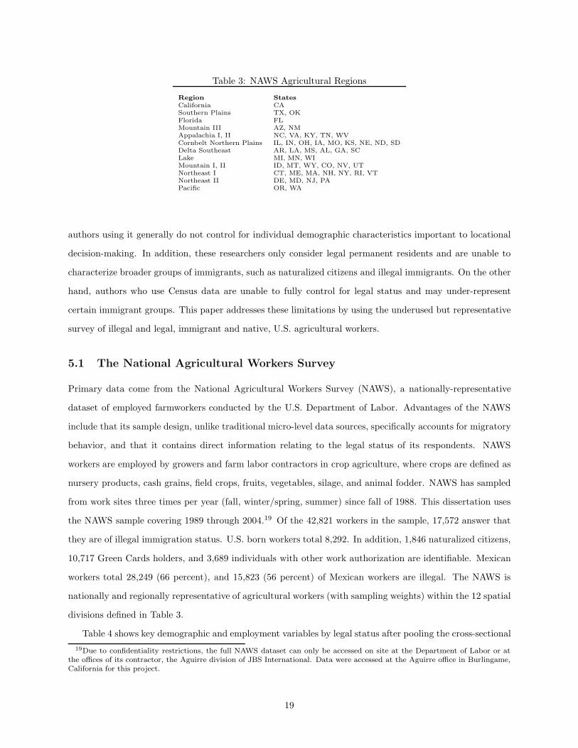
Table 3: NAWS Agricultural Regions

Region StatesCalifornia CASouthern Plains TX, OKFlorida FLMountain III AZ, NMAppalachia I, II NC, VA, KY, TN, WVCornbelt Northern Plains IL, IN, OH, IA, MO, KS, NE, ND, SDDelta Southeast AR, LA, MS, AL, GA, SCLake MI, MN, WIMountain I, II ID, MT, WY, CO, NV, UTNortheast I CT, ME, MA, NH, NY, RI, VTNortheast II DE, MD, NJ, PAPacific OR, WA

authors using it generally do not control for individual demographic characteristics important to locational

decision-making. In addition, these researchers only consider legal permanent residents and are unable to

characterize broader groups of immigrants, such as naturalized citizens and illegal immigrants. On the other

hand, authors who use Census data are unable to fully control for legal status and may under-represent

certain immigrant groups. This paper addresses these limitations by using the underused but representative

survey of illegal and legal, immigrant and native, U.S. agricultural workers.

5.1 The National Agricultural Workers Survey

Primary data come from the National Agricultural Workers Survey (NAWS), a nationally-representative

dataset of employed farmworkers conducted by the U.S. Department of Labor. Advantages of the NAWS

include that its sample design, unlike traditional micro-level data sources, specifically accounts for migratory

behavior, and that it contains direct information relating to the legal status of its respondents. NAWS

workers are employed by growers and farm labor contractors in crop agriculture, where crops are defined as

nursery products, cash grains, field crops, fruits, vegetables, silage, and animal fodder. NAWS has sampled

from work sites three times per year (fall, winter/spring, summer) since fall of 1988. This dissertation uses

the NAWS sample covering 1989 through 2004.19 Of the 42,821 workers in the sample, 17,572 answer that

they are of illegal immigration status. U.S. born workers total 8,292. In addition, 1,846 naturalized citizens,

10,717 Green Cards holders, and 3,689 individuals with other work authorization are identifiable. Mexican

workers total 28,249 (66 percent), and 15,823 (56 percent) of Mexican workers are illegal. The NAWS is

nationally and regionally representative of agricultural workers (with sampling weights) within the 12 spatial

divisions defined in Table 3.

Table 4 shows key demographic and employment variables by legal status after pooling the cross-sectional19Due to confidentiality restrictions, the full NAWS dataset can only be accessed on site at the Department of Labor or at

the offices of its contractor, the Aguirre division of JBS International. Data were accessed at the Aguirre office in Burlingame,California for this project.

19

Table 4: Means of Key Demographic and Employment Variables, by Legal Status

Native Illegal Nat. Green OtherCitizen Card Author.

Female (%) 36.70 15.52 18.47 23.19 13.67Age (yrs) 32.41 27.58 38.73 38.08 31.46Married, spouse in U.S. (%) 42.34 18.42 46.38 56.67 33.55Married, spouse anywhere (%) 44.73 46.28 61.02 76.17 63.67Children in U.S. (#) 0.75 0.37 1.07 1.35 0.93None (%) 64.72 83.08 58.17 48.14 65.86One (%) 12.57 6.45 9.24 12.08 10.12More than one (%) 22.72 10.46 32.59 39.78 24.02Children anywhere (#) 0.79 0.93 1.23 1.74 1.01Education (yrs) 10.70 6.22 7.53 5.89 5.51U.S. farmwork experience (yrs) 13.46 4.12 16.46 15.49 9.53Hourly wage ($1982-4) 4.02 3.70 4.07 4.10 4.06Speaks English (%) 94.86 7.31 42.53 22.54 16.31Reads English (%) 93.11 5.65 34.84 18.19 11.73Has work network (%) 56.61 77.84 61.71 59.73 62.34Paid below min wage (%) 7.62 12.74 7.27 6.64 7.48Hispanic (%) 35.95 98.59 94.95 96.56 98.27in California (%) 7.08 33.76 24.73 51.39 35.01in Southern Plains (TX, OK) (%) 9.76 2.76 6.52 7.71 5.43in Florida (%) 3.08 7.87 13.02 5.01 8.20in Arizona or New Mexico (%) 0.87 1.66 1.83 4.24 3.21from Mexico (%) 93.73 51.20 94.72 94.87Observations 5664 16514 1598 9622 2547

Source: National Agricultural Workers Survey, pooled cross sections 1989-2004.

data. Immigrants working in agriculture are more likely to be male than are U.S. born citizens. Legal

immigrants are older on average than natives, and illegal immigrants are younger. Immigrants have fewer

years of education and are less likely to report English language ability. Illegal immigrants report fewer

years of U.S. experience than do legal immigrants.20 In terms of locational distributions across U.S. regions,

immigrants are more likely to reside in California, Florida, or the Arizona/New Mexico region than are their

native counterparts. The opposite is true of Southern Plains (TX, OK) farmworkers.21

In some sense, the data represent a compromise in order to say anything about the often transparent

population of illegal immigrants. Although the agricultural industry is a major player in the overall labor

market for illegal workers, using the NAWS for a study of migration, specifically illegal migration, has its

limitations. Because NAWS is a survey only of farmworkers, those employed in other sectors of the economy

and the unemployed are excluded. An additional consideration is that since the survey relies on end-point

sampling within the destination country, data are only representative of successful border crossers. Thirdly,

workers are observed only once, and it is uncertain to what extent observed locations correspond to points

of entry.

Welfare participation rates by region are presented in Table 1. California and Florida represent their

own regions. Texas is grouped with Oklahoma, and Arizona with New Mexico. These four regions, repre-

senting the border states and key U.S. agricultural players, are compared with an inclusive “other” category20The experience variable is calculated as survey year minus reported first year of U.S. farmwork.21Unfortunately, the NAWS does not survey workers in agriculture-related occupations such as livestock. This may account

for the low percentages of Southern Plains respondents.

20

comprising workers from the remaining eight regions.

One previous paper using the NAWS is directly related to this one. Moretti and Perloff (2000) examine

farmworkers’ welfare program and private charity take-up decisions. The authors find that illegal immigrant

families are more likely to use public medical assistance and less likely to use other public aid programs when

compared with legal immigrants and U.S. born citizens. In addition, they show a positive correlation between

public aid participation and U.S. born children in households headed by illegal immigrants. Although they

do not consider geographic clustering, their paper has implications for this study. If welfare migration

does exist, it may be stronger along the dimension of medical service or among those with certain family

structures.

5.2 Locational Clustering of Public Aid Participants in the NAWS

As documented in Table 1, participation rates vary both across legal status and across states. Table 5 exam-

ines geographic clustering of NAWS households that have received aid in California, Texas, Florida, Arizona

and other states. In the absence of welfare clustering, roughly equal percentages of welfare participants and

nonparticipants would be expected to reside in each state. For example, if 30 percent of U.S. welfare partici-

pants live in California, then 30 percent of nonparticipants should also live there. Likewise, equal percentages

of participants and nonparticipants in each legal status/state category are expected. The difference between

the percentage of participant households living in state s and the percentage of nonparticipant households

in state s is an unconditional estimate of the “welfare clustering gap” associated with that location. Table

5 presents percentages of NAWS households who participated and who did not participate in public aid

programs in the last two years by legal status and region of residence. A two sample t-test of the equality of

means between participant and nonparticipant percentages is an unconditional test for evidence of a welfare

clustering gap.

The California panel of Table 5 shows that almost 30 percent of the U.S. farmworkers who received some

form of aid lived in California while just over 29 percent of those who did not receive aid resided there. The

difference is not statistically significant, discrediting the existence of overall welfare clustering in California

in the raw data. The significant differences that do appear in the California panel of Table 5 correspond

to U.S. born workers, naturalized citizens, and Green Card holders. The data suggests a positive welfare

clustering gap for the U.S. born population in California. Of the full sample of native farmworkers who use

aid anywhere in the country, 7.26 percent live in California, but only 4.41 percent of native farmworkers

who do not use aid live there. Higher percentages of nonparticipating households than participating ones

are observed among naturalized citizens and Green Card holders in California, indicating the absence of a

21

Table 5: Geographic Clustering of Welfare Recipients (percentage of households)

California migrantshave have not t-testused welfare used welfare equality p-value

Full sample 29.98 29.40 -0.73 0.47Natives 7.26 4.41 -3.10 0.00Naturalized citizens 19.30 26.21 2.60 0.01Green Card 48.91 52.11 1.93 0.05Other work authorization 34.13 35.82 0.54 0.59Illegal immigrants 31.10 33.02 1.24 0.21

Southern Plains (Texas, OK) migrantshave have not t-testused welfare used welfare equality p-value

Full sample 9.37 4.18 -9.48 0.00Natives 12.71 5.41 -5.98 0.00Naturalized citizens 8.43 4.54 -2.05 0.04Green Card 10.51 5.81 -4.17 0.00Other work authorization 9.83 5.69 -2.38 0.02Illegal immigrants 4.88 2.60 -3.28 0.00

Florida migrantshave have not t-testused welfare used welfare equality p-value

Full sample 6.34 6.84 1.04 0.30Natives 4.35 3.02 -2.52 0.01Naturalized citizens 7.66 16.13 4.49 0.00Green Card 6.45 5.23 -1.02 0.31Other work authorization 10.54 8.19 -1.30 0.20Illegal immigrants 6.90 8.54 2.39 0.02

Mountain III (Arizona, NM) migrantshave have not t-testused welfare used welfare equality p-value

Full sample 1.32 2.36 6.78 0.00Natives 0.53 0.66 0.64 0.52Naturalized citizens 1.76 1.64 -0.18 0.86Green Card 1.97 5.36 8.35 0.00Other work authorization 1.59 4.08 4.56 0.00Illegal immigrants 0.88 1.81 3.94 0.00

Other U.S. Region migrantshave have not t-testused welfare used welfare equality p-value

Full sample 53.00 57.22 4.36 0.00Natives 75.14 86.50 7.20 0.00Naturalized citizens 62.86 51.48 -3.21 0.00Green Card 32.16 31.49 -0.41 0.68Other work authorization 43.92 46.23 0.60 0.55Illegal immigrants 56.24 54.03 -1.25 0.21

Source: National Agricultural Workers Survey, pooled cross sections 1989-2004.

22

welfare clustering gap for these legal status groups in the raw data.22

For the Southern Plains, all subgroups display significant differences between participants and nonpar-

ticipants. Participants are unconditionally more likely to be observed in the Southern Plains than are

nonparticipants. This is true across legal status groups. Also notable is the Arizona/New Mexico category,

for which patterns are largely opposite of those for the Southern Plains. Florida presents an intermediate

case.

The statistics presented in Table 5 do not control for socioeconomic characteristics, and therefore might

reflect differences in the distributions of characteristics associated with participation across state instead of

behavioral clustering. To further describe the participation data, an empirical test for the existence of a

welfare clustering gap using multivariate regression analysis is developed.

5.3 Empirical Test of the Existence of a Welfare Clustering Gap

The probability of locating in state s (Ps) is assumed to be an increasing function of expected net benefits

and is defined:

Ps = Pr(Us > Us′ , ∀s′ ∈ S, s �= s′) (10)

where

Us = Vs + εs (11)

Utility from migrating to s (Us) comprises two components, a systematic utility term (Vs) and a random

error term (εs). As in the theoretical section, migrants select the location offering the highest value.

Borjas (1999) develops a descriptive linear probability model in which the probability of residing in

California, his welfare magnet candidate, is regressed on a welfare participation indicator, an immigrant

indicator, their interaction, and socioeconomic controls. His regression is of the form:

CAi = X ′iγ + α1Immigranti + α2Bi + α3(Immigranti × Bi) + εi (12)

CAi is a dummy variable corresponding to one if the survey respondent was observed in California. Xi

is a vector of socioeconomic characteristics including gender, age, presence of spouse, number of children,

years of education, and years of U.S. farm experience. Bi indicates if individual i (or i ’s family) is a public

aid participant. The coefficient α3 is an estimator of the welfare clustering gap in California. The welfare22The welfare clustering gap definition in this section is the presence of a positive difference between the percentage of

participant households locating in state s and the percentage of non-participant households locating there. Higher percentagesof residents drawn from the non-participant distribution than from the participant distribution is evidence against the existenceof a welfare clustering gap for that state.

23

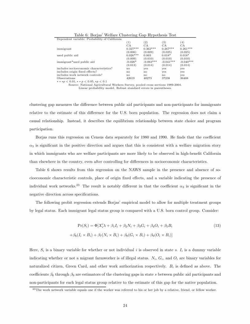
Table 6: Borjas’ Welfare Clustering Gap Hypothesis TestDependent variable: Probability of California

(1) (2) (3) (4)CA CA CA CA

immigrant 0.327*** 0.362*** 0.267*** 0.261***(0.006) (0.009) (0.025) (0.025)

used public aid 0.026*** 0.003 0.018* 0.018*(0.009) (0.010) (0.010) (0.010)

immigrant*used public aid -0.026* -0.063*** -0.041*** -0.040***(0.013) (0.014) (0.014) (0.014)

includes socioeconomic characteristics? no yes yes yesincludes origin fixed effects? no no yes yesincludes work network controls? no no no yesObservations 42619 40273 37238 36408∗ ∗ ∗p < 0.01, ∗ ∗ p < 0.05, ∗p < 0.1

Source: National Agricultural Workers Survey, pooled cross sections 1989-2004.Linear probability model. Robust standard errors in parentheses.

clustering gap measures the difference between public aid participants and non-participants for immigrants

relative to the estimate of this difference for the U.S. born population. The regression does not claim a

causal relationship. Instead, it describes the equilibrium relationship between state choice and program

participation.

Borjas runs this regression on Census data separately for 1980 and 1990. He finds that the coefficient

α3 is significant in the positive direction and argues that this is consistent with a welfare migration story

in which immigrants who are welfare participants are more likely to be observed in high-benefit California

than elsewhere in the country, even after controlling for differences in socioeconomic characteristics.

Table 6 shows results from this regression on the NAWS sample in the presence and absence of so-

cioeconomic characteristic controls, place of origin fixed effects, and a variable indicating the presence of

individual work networks.23 The result is notably different in that the coefficient α3 is significant in the

negative direction across specifications.

The following probit regression extends Borjas’ empirical model to allow for multiple treatment groups

by legal status. Each immigrant legal status group is compared with a U.S. born control group. Consider:

Pr(Si) = Φ[X ′iλ + β1Ii + β2Ni + β3Gi + β4Oi + β5Bi (13)

+β6(Ii × Bi) + β7(Ni × Bi) + β8(Gi × Bi) + β9(Oi × Bi)]

Here, Si is a binary variable for whether or not individual i is observed in state s. Ii is a dummy variable

indicating whether or not a migrant farmworker is of illegal status. Ni, Gi, and Oi are binary variables for

naturalized citizen, Green Card, and other work authorization respectively. Bi is defined as above. The

coefficients β6 through β9 are estimators of the clustering gaps in state s between public aid participants and

non-participants for each legal status group relative to the estimate of this gap for the native population.23The work network variable equals one if the worker was referred to his or her job by a relative, friend, or fellow worker.

24

Table 7: Welfare Clustering Gap Hypothesis Test RevisedDependent variable: Probability of State s

(1) (2) (3) (4) (5)CA TX FL AZ Other

naturalized citizen 0.446*** -0.021*** 0.066** -0.001 -0.324***(0.041) (0.003) (0.027) (0.003) (0.038)

Green Card 0.512*** -0.029*** 0.034** 0.004 -0.396***(0.030) (0.004) (0.016) (0.004) (0.030)

other work author. 0.384*** -0.022*** 0.066*** 0.008 -0.257***(0.041) (0.002) (0.025) (0.007) (0.040)

illegal 0.350*** -0.062*** 0.049*** 0.002 -0.269***(0.026) (0.010) (0.013) (0.003) (0.033)

used public aid 0.073*** 0.031*** 0.013* -0.001 -0.159***(0.024) (0.007) (0.007) (0.002) (0.023)

naturalized*used public aid -0.078** -0.014*** -0.030*** 0.002 0.219***(0.034) (0.005) (0.004) (0.005) (0.036)

Green Card*used public aid -0.072*** -0.012*** 0.002 -0.003** 0.145***(0.023) (0.004) (0.011) (0.001) (0.026)

other author.*used public aid -0.085** 0.001 -0.004 -0.003** 0.117**(0.035) (0.011) (0.012) (0.001) (0.054)

illegal*used public aid -0.122*** -0.011*** -0.019*** -0.003*** 0.230***(0.018) (0.004) (0.005) (0.001) (0.022)

Observations 35967 34884 35967 35898 35967**** p < 0.01, ** p < 0.05, * p < 0.1

Source: National Agricultural Workers Survey, pooled cross sections 1989-2004.Probit marginal effects. Robust standard errors in parentheses.

The characteristics in Xi control for demographic factors associated with program eligibility (e.g. family

structure) and for systematic differences in the averages of these factors across legal status groups.24 National

or regional origin effects are included in reported specifications. Previous papers (e.g. Zavodny (1999), Borjas

(1999), Dodson (2001)) use immigrant country of origin to control for linguistic and cultural networks. The

NAWS allows for the opportunity to refine this to the state level within the country of origin. Due to low

sample sizes from sending countries other than Mexico, state-level origin controls only are used in the case

of Mexico. National-level origin controls are used for those from countries besides Mexico. Survey year and

season fixed effects are included in all regressions.

Table 7 presents estimates of the clustering gaps between welfare participants and nonparticipants for the

four immigrant legal status groups relative to natives in separate regressions for California, Texas, Florida,

Arizona, and other U.S. states.25 Negative coefficients on legal status/participation interactions indicate

that there no evidence of welfare clustering relative to the U.S. born population. Using similar methodology,

Borjas (1999) finds strong positive welfare clustering in California by legal immigrants relative to natives.

As evident in Column (1) of Table 7, no such results are found for any legal status group in California for

this analysis using the NAWS.26 Instead, naturalized citizens who use public aid are 7.8 percent less likely to24Income, which may be associated with eligibility for aid programs, is not explicitly accounted for in this framework. Given

that the sample comprises farm laborers who are low income irrespective of legal status group, this is less of a concern than itwould be for higher income persons who are excluded from participating. Borjas (1999) discusses a second issue surroundingincome. Higher relative benefits cover larger ranges of the distribution of reservation incomes than do lower benefits, andthe estimation method may integrate over different distributions even for members of various legal status groups who areobservationally equivalent. In the theoretical model of Section 3, public aid is assumed to be a supplement to income, asopposed to a replacement of income, thus minimizing this concern.

25From this point forward, “Texas” refers to the “Southern Plains” and “Arizona” to Arizona/New Mexico.26It should be noted again that all NAWS respondents are employed (at least part-time) by definition. Robustness analysis

25

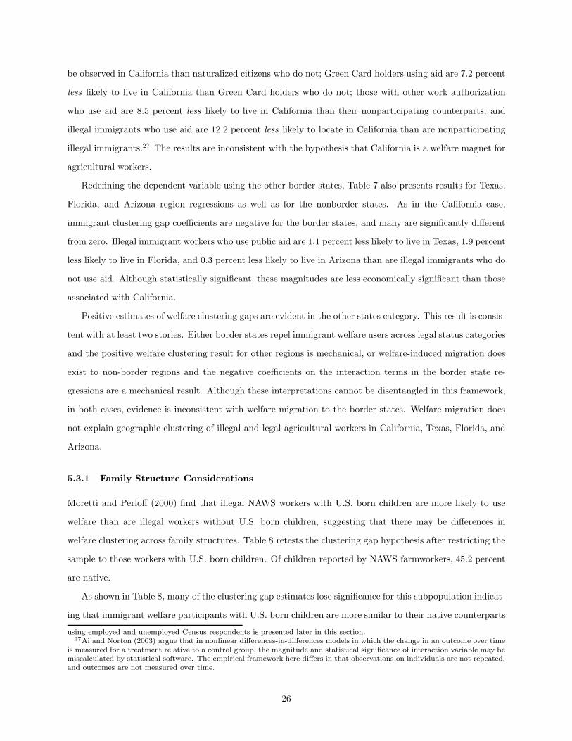
be observed in California than naturalized citizens who do not; Green Card holders using aid are 7.2 percent

less likely to live in California than Green Card holders who do not; those with other work authorization

who use aid are 8.5 percent less likely to live in California than their nonparticipating counterparts; and

illegal immigrants who use aid are 12.2 percent less likely to locate in California than are nonparticipating

illegal immigrants.27 The results are inconsistent with the hypothesis that California is a welfare magnet for

agricultural workers.

Redefining the dependent variable using the other border states, Table 7 also presents results for Texas,

Florida, and Arizona region regressions as well as for the nonborder states. As in the California case,

immigrant clustering gap coefficients are negative for the border states, and many are significantly different

from zero. Illegal immigrant workers who use public aid are 1.1 percent less likely to live in Texas, 1.9 percent

less likely to live in Florida, and 0.3 percent less likely to live in Arizona than are illegal immigrants who do

not use aid. Although statistically significant, these magnitudes are less economically significant than those

associated with California.

Positive estimates of welfare clustering gaps are evident in the other states category. This result is consis-

tent with at least two stories. Either border states repel immigrant welfare users across legal status categories

and the positive welfare clustering result for other regions is mechanical, or welfare-induced migration does

exist to non-border regions and the negative coefficients on the interaction terms in the border state re-

gressions are a mechanical result. Although these interpretations cannot be disentangled in this framework,

in both cases, evidence is inconsistent with welfare migration to the border states. Welfare migration does

not explain geographic clustering of illegal and legal agricultural workers in California, Texas, Florida, and

Arizona.

5.3.1 Family Structure Considerations

Moretti and Perloff (2000) find that illegal NAWS workers with U.S. born children are more likely to use

welfare than are illegal workers without U.S. born children, suggesting that there may be differences in

welfare clustering across family structures. Table 8 retests the clustering gap hypothesis after restricting the

sample to those workers with U.S. born children. Of children reported by NAWS farmworkers, 45.2 percent

are native.

As shown in Table 8, many of the clustering gap estimates lose significance for this subpopulation indicat-

ing that immigrant welfare participants with U.S. born children are more similar to their native counterparts

using employed and unemployed Census respondents is presented later in this section.27Ai and Norton (2003) argue that in nonlinear differences-in-differences models in which the change in an outcome over time

is measured for a treatment relative to a control group, the magnitude and statistical significance of interaction variable may bemiscalculated by statistical software. The empirical framework here differs in that observations on individuals are not repeated,and outcomes are not measured over time.

26

Table 8: Farmworkers with U.S. Born Children Clustering Gap TestDependent variable: Probability of State s

(1) (2) (3) (4) (5)CA TX FL AZ Other

naturalized citizen 0.432*** -0.022*** 0.040 -0.000 -0.236***(0.088) (0.003) (0.042) (0.009) (0.086)

Green Card 0.493*** -0.024*** 0.009 0.004 -0.327***(0.062) (0.008) (0.022) (0.010) (0.068)

other work author. 0.313*** -0.020*** 0.019 0.005 -0.118(0.093) (0.004) (0.029) (0.013) (0.093)

illegal 0.333*** -0.042*** 0.029 0.000 -0.220***(0.053) (0.015) (0.020) (0.008) (0.070)

used public aid 0.083** 0.018* 0.011 -0.005 -0.130***(0.041) (0.010) (0.014) (0.003) (0.043)

naturalized*used public aid -0.059 -0.000 -0.031*** 0.001 0.186***(0.067) (0.018) (0.007) (0.010) (0.071)

Green Card*used public aid -0.072* -0.012* 0.011 -0.002 0.114**(0.041) (0.006) (0.025) (0.004) (0.050)

other author.*used public aid -0.053 0.023 0.017 0.003 0.002(0.079) (0.034) (0.030) (0.012) (0.108)

illegal*used public aid -0.118*** -0.008 -0.019* -0.002 0.205***(0.030) (0.008) (0.010) (0.004) (0.042)



than are those without U.S. born children. The coefficients on the interaction terms between participation

and legal status for the three legal immigrant groups relative to natives are not significantly different from

zero in most cases, but illegal immigrant households with U.S. born children who use welfare are still almost

12 percent less likely to live in California than are their native counterparts, suggesting that the California

results are not driven by systematic family structure differences across states.

5.3.2 California Proposition 187 and PRWORA

The strong negative clustering gap coefficients in the California regression deserve additional consideration.

As mentioned, California was the stage for multiple immigration and public aid related policy changes

throughout the NAWS sample period. Table 9 considers welfare clustering gaps for California in three periods.

The first period, 1989 to 1994, predates California Proposition 187, which eliminated welfare, education,

and medical service eligibility for illegal immigrants. The second period, 1995 to 1996, corresponds to the

period between the enactment of Proposition 187 and PRWORA.28 The third, 1997 to 2004, is subsequent to

federal welfare reform. The coefficients corresponding to the clustering gap for illegal immigrants over natives

reflect these policy changes. Referring to the interaction term, before Proposition 187, illegal households

in agriculture who used aid programs were 5.6 percent less likely to reside in California than were illegal

households who did not use aid. In the Proposition 187 period, illegal participants were 16.3 percent less

likely than their nonparticipating counterparts to be observed in California, and in the post-1996 welfare28Since Proposition 187 was in effect from November 1994 until November 1995, the 1995 to 1996 data are pooled for this

exercise. This is appropriate given that the survey question asks if the respondent or his or her family participated in publicaid programs within the last two years.

27

Table 9: California Clustering Gap TestDependent variable: Probability of California

1989-1994 1995-1996 1997-2004(1) (2) (3)CA CA CA

naturalized citizen 0.579*** 0.350** 0.394***(0.078) (0.143) (0.053)

Green Card 0.609*** 0.582*** 0.433***(0.053) (0.068) (0.042)

other work author. 0.475*** 0.162 0.195**(0.065) (0.116) (0.084)

illegal 0.347*** 0.366*** 0.325***(0.050) (0.065) (0.036)

used public aid 0.049* 0.121** 0.060(0.028) (0.061) (0.038)

naturalized*used public aid -0.064* -0.027 -0.087*(0.036) (0.136) (0.052)

Green Card*used public aid -0.062*** -0.086* -0.074*(0.022) (0.052) (0.039)

other author.*used public aid -0.030 -0.142** -0.097(0.039) (0.068) (0.084)

illegal*used public aid -0.056** -0.163*** -0.141***(0.026) (0.037) (0.030)

Observations 8376 4127 23463**** p < 0.01, ** p < 0.05, * p < 0.1

Source: National Agricultural Workers Survey, pooled cross sections 1989-1994, 1995-1996, and 1997-2004.Probit marginal effects. Robust standard errors in parentheses.

reform period, this number is 14.1 percent. While illegal immigrants who use public aid were less likely to

be in California than nonparticipants and natives before 1994, decreased participation by illegal farmworkers

is observed during the Proposition 187 period. Results for regressions considering the pre- and post-1996

federal welfare reform periods for alternate destination states are similar and are not reported.

5.3.3 Food, Medical, and Insurance Programs

Camarota (2004) finds that due to individual program eligibility restrictions, illegal immigrants are more

likely to use food assistance and medical programs than cash-transfers. Table 10 presents estimates of

clustering gaps associated with specific aid programs, and the results parallel those for the full sample. Food

aid consisting of FSP and WIC is presented in the top panel. The second panel presents results corresponding

to a medical assistance category comprising Medicaid and public health center services. The third presents

Social Security and disability insurance.

Even with these revised definitions, there is little evidence supporting welfare clustering in border states

for agricultural workers. The difference in propensity to choose California between illegal immigrants who use

aid and those who do not is strongest for medical care programs. Illegal immigrants who use medical services

are 12.1 percent less likely to locate in California than illegal immigrants who do not. Illegal immigrants who

use social insurance programs or food aid are 10.7 and 8.4 percent less likely respectively to live in California

than are their nonparticipating counterparts. The negative significant welfare clustering gap estimates for

the Texas and Florida regressions in Table 7 appear primarily driven by food aid participation, while that

28

Table 10: Food, Medical, and Insurance Program Clustering Gap TestsDependent variable: Probability of State s

(1) (2) (3) (4) (5)CA TX FL AZ Other

Food Aid (food stamps or WIC):naturalized*used program -0.090** -0.018*** -0.027*** 0.007 0.235***

(0.037) (0.004) (0.005) (0.008) (0.036)Green Card*used program -0.071*** -0.008* 0.006 -0.001 0.155***

(0.025) (0.005) (0.013) (0.002) (0.027)other author.*used program -0.042 -0.009 -0.002 -0.002 0.1

(0.046) (0.008) (0.013) (0.002) (0.061)illegal*used program -0.084*** -0.015*** -0.021*** -0.002 0.221***

(0.022) (0.004) (0.005) (0.002) (0.024)Medical (Medicaid or public health):naturalized*used program -0.038 -0.012* -0.027*** 0.005 0.143***

(0.051) (0.006) (0.006) (0.008) (0.052)Green Card*used program -0.049 -0.013*** 0.008 -0.004*** 0.086**

(0.034) (0.004) (0.016) (0.001) (0.035)other author.*used program -0.114** 0.002 0.000 -0.002 0.124

(0.054) (0.019) (0.027) (0.004) (0.087)illegal*used program -0.121*** -0.007 -0.016** -0.005*** 0.202***

(0.025) (0.005) (0.007) (0.001) (0.030)Social Security or disability insurance:naturalized*used program -0.044 0.018 -0.023** 0.052 0.027

(0.065) (0.028) (0.010) (0.041) (0.086)Green Card*used program -0.003 -0.013* -0.026*** 0.055 0.074

(0.042) (0.007) (0.007) (0.034) (0.056)other author.*used program 0.136 -0.005 -0.018 -0.003 -0.013

(0.102) (0.015) (0.013) (0.003) (0.110)illegal*used program -0.107** -0.005 -0.015 0.083 0.155**

(0.047) (0.012) (0.016) (0.059) (0.069)*** p < 0.01, ** p < 0.05, * p < 0.1


for Arizona is most related to medical services.

5.3.4 Education

The NAWS affords the opportunity to consider how education program availability affects locational choice.

A long literature in public finance and education is devoted to Tiebout choice, or geographic sorting of

individuals based on preferences over a set of available public good bundles, and its potential outcomes for

students, parents, and communities. Public education is costly to state government and whether it should

be available to illegal immigrants is a subject of heated debate. NAWS respondents were asked if they

or members of their family participated in any of a number of U.S. educational programs in the last two

years, including English as a Second Language, basic education, citizenship, job training, GED/high school

equivalence, migrant education, Head Start, and Migrant Head Start.

Table 11 presents estimates of education clustering gaps. Again, a series of probits are presented in

which the dependent variable is the probability of residing in state s. Few clustering gap interactions in this

category are significantly different from zero. Illegal immigrants who use schools, however, are less likely to

reside in California and more likely to reside in other U.S. regions.

Because adult immigrants may use educational programs to a lesser extent than their children do, Table

29

Table 11: Education Clustering Gap TestDependent variable: Probability of State s

(1) (2) (3) (4) (5)CA TX FL AZ Other

naturalized citizen 0.418*** -0.019*** 0.032 -0.003 -0.261***(0.046) (0.003) (0.025) (0.003) (0.044)

Green Card 0.487*** -0.025*** 0.027 0.004 -0.380***(0.035) (0.005) (0.019) (0.006) (0.037)

other work author. 0.271*** -0.011* 0.030 -0.001 -0.168***(0.058) (0.006) (0.028) (0.005) (0.057)

illegal 0.313*** -0.062*** 0.025 0.002 -0.181***(0.032) (0.010) (0.015) (0.005) (0.041)

used schools -0.035 -0.001 0.006 0.002 0.012(0.035) (0.006) (0.011) (0.004) (0.035)

naturalized*public education -0.038 -0.010 -0.019** 0.013 0.077(0.063) (0.013) (0.009) (0.015) (0.074)

Green Card*public education -0.041 -0.007 0.001 -0.002 0.097**(0.041) (0.007) (0.015) (0.003) (0.041)

other author.*public education 0.028 -0.015** 0.010 -0.000 0.002(0.099) (0.007) (0.027) (0.006) (0.105)

illegal*public education -0.090** 0.022 -0.002 0.001 0.090**(0.035) (0.014) (0.011) (0.005) (0.044)



Table 12: Child Education Clustering Gap TestDependent variable: Probability of State s

(1) (2) (3) (4) (5)CA TX FL AZ Other

naturalized citizen 0.417*** -0.025*** 0.039 -0.006** -0.173*(0.088) (0.003) (0.047) (0.002) (0.090)

Green Card 0.371*** -0.037*** 0.052 0.001 -0.204***(0.069) (0.008) (0.033) (0.007) (0.072)

other work author. 0.302*** -0.013 0.037 -0.003 -0.141(0.110) (0.012) (0.039) (0.005) (0.110)

illegal 0.282*** -0.061*** 0.018 -0.002 -0.103(0.054) (0.019) (0.021) (0.007) (0.070)

used public aid -0.015 -0.018* 0.013 -0.016* 0.077*(0.035) (0.009) (0.011) (0.009) (0.040)

naturalized*public education -0.011 0.036 -0.025** 0.085 -0.016(0.069) (0.042) (0.012) (0.098) (0.086)

Green Card*public education 0.094* 0.023 -0.039*** 0.016 -0.108**(0.052) (0.015) (0.009) (0.013) (0.052)

other author.*public education -0.059 -0.015 -0.021 0.064 0.056(0.076) (0.011) (0.013) (0.051) (0.109)

illegal*public education -0.001 0.012 -0.004 0.012 -0.060(0.039) (0.011) (0.014) (0.008) (0.046)



30

12 restricts the sample to agricultural workers with children. The public education participation variable

is redefined as the response to a more specific question as to whether a child of the farmworker attended

school within the last year. Of the 26,982 children represented in NAWS responses, 66 percent used schools

in the last year. Few of the clustering gap estimates are statistically significantly different from zero. This

is consistent with children of illegal and legal immigrants attending school roughly as frequently as children

of U.S. born parents do.

5.4 Welfare Clustering in the U.S. Census

Because the NAWS is a survey of agricultural workers, the question arises as to whether the results are

generalizable to the rest of the population and how these results can be reconciled with those of Borjas

(1999). The Census does not distinguish illegal from legal immigrants. Instead, the only citizenship-related

question asked to immigrants is whether they are naturalized citizens. Thus, naturalized citizens can be

distinguished from noncitizens, but legal permanent residents cannot be distinguished from illegal persons,

and within the legal permanent resident category, Green Card holders cannot be distinguished from those

with other work authorization. The broadest definition of welfare benefits available in the Census is used

here, which is based on usage of TANF, FSP, or SSI within the last year. Thus, the welfare participation

variable is more restrictive (both temporally and in terms of program specificity) than that used in the

analysis using the NAWS.

Borjas (1999) finds that welfare recipients cluster in benefit-generous California using 1980 and 1990 Cen-

sus data. The 2000 Census is the first available decennial Census in the post-PRWORA period. Therefore, it

is useful to establish if the patterns Borjas observed are still evident after changes in eligibility requirements.

Column (1) of Table 13 confirms Borjas’ result using the latest Census data: the welfare clustering gaps

of naturalized citizens and of noncitizens relative to the U.S. born population are positive and significant.

Naturalized citizens who used public aid were 2.2 percent more likely to be observed in California than were

U.S. born welfare participants, and noncitizen participants were 7.7 percent more likely to be observed in

California than were native participants.

One difference between the NAWS and the Census is that NAWS only includes employed persons in

agriculture, while the Census is representative of both those in the labor force and those apart from it. If

Borjas’ result is driven by welfare use by unemployed persons then this would explain the conflicting evidence

using like-methodology with the NAWS data. Column (2) of Table 13 restricts the U.S. Census sample to

those active in the labor force.29 Borjas’ result still holds. The clustering gap estimate for unemployed29In 2000, the reference period for this question was one week. Respondents were asked if they worked for pay last week. If

the response was negative, additional questions examined if this was a temporary situation.

31

Table 13: 2000 Census Clustering Gap TestDependent variable: Probability of California

full sample in labor unemployed not in laborforce force

(1) (2) (3) (4)CA CA CA CA

naturalized citizen 0.072*** 0.060*** 0.075*** 0.092***(0.003) (0.003) (0.016) (0.005)

noncitizen 0.071*** 0.058*** 0.072*** 0.098***(0.002) (0.002) (0.011) (0.004)

used public aid 0.027*** 0.016*** 0.005 0.031***(0.002) (0.006) (0.015) (0.002)

naturalized*used public aid 0.022*** 0.090*** 0.029 -0.014*(0.008) (0.018) (0.033) (0.007)

noncitizen*used public aid 0.077*** 0.077*** 0.115*** 0.049***(0.008) (0.013) (0.031) (0.010)

Observations 1054372 685641 26022 342709*** p < 0.01, ** p < 0.05, * p < 0.1

Source: 2000 U.S. Census, 1% sample of full population.Probit marginal effects. Robust standard errors in parentheses.

Table 14: 1990 Census Clustering Gap Test – FarmworkersDependent variable: Probability of State s

(1) (2) (3) (4) (5)CA TX FL AZ Other

naturalized citizen -0.036 -0.013 -0.011 0.976*** 0.111(0.038) (0.035) (0.028) (0.004) (0.080)

noncitizen 0.025 -0.051* -0.028 0.957*** 0.066(0.050) (0.027) (0.022) (0.002) (0.089)

used public aid 0.026** -0.009 -0.010** -0.006** 0.007(0.012) (0.008) (0.005) (0.003) (0.015)

naturalized*used public aid -0.025 0.071* -0.029** 0.004 -0.038(0.029) (0.042) (0.012) (0.012) (0.087)

noncitizen*used public aid -0.025 0.089*** -0.038*** 0.001 -0.047(0.018) (0.029) (0.005) (0.008) (0.046)


Source: 1990 U.S. Census, 5% sample of farm laborers.Probit marginal effects. Robust standard errors in parentheses.

Table 15: 2000 Census Clustering Gap Test – FarmworkersDependent variable: Probability of State s

(1) (2) (3) (4) (5)CA TX FL AZ Other

naturalized citizen -0.037 -0.023 -0.003 0.002 0.125(0.048) (0.033) (0.032) (0.013) (0.101)

noncitizen -0.004 -0.039 -0.007 0.007 0.091(0.054) (0.033) (0.032) (0.014) (0.111)

used public aid 0.098*** -0.002 0.011 -0.006 -0.082***(0.019) (0.010) (0.008) (0.004) (0.020)

naturalized*used public aid -0.063** 0.049 -0.031*** 0.011 0.006(0.026) (0.035) (0.010) (0.016) (0.059)

noncitizen*used public aid -0.061*** 0.065** -0.019* -0.008 0.021(0.017) (0.027) (0.011) (0.006) (0.035)


Source: 2000 U.S. Census, 5% sample of farm laborers.Robust standard errors in parentheses.

32

persons (Column (3)), however, is more pronounced than that for employed persons. Unemployed noncitizen

welfare participants are 11.5 percent more likely to be observed in California than are unemployed U.S. born

welfare participants, while employed noncitizen participants are 7.7 percent more likely to be in California

than are employed U.S. born participants.

Occupation-related questions in the Census allow farm laborers to be identified. Because farm laborers

in the Census are a relatively small sample (partially due to undersampling as noted earlier), the five percent

version of both the 1990 and 2000 Census is used to repeat the exercise and to check for differences before

and after PRWORA. Tables 14 and 15 present the results. The negative welfare clustering gaps across legal

status groups found using the NAWS also appear using this subsample. Therefore, while unemployed workers

may still engage in welfare migration (as suggested by positive clustering gap estimates for immigrants in

the overall Census results), the difference between the results using the NAWS and those in Borjas (1999)

are not primarily due to differences between the unemployed and the employed. Instead, the similar results

when using Census agricultural workers and when using the NAWS suggest that differences between the main

results in Borjas (1999) and this paper are due to a fundamental difference between agricultural workers and

the rest of the immigrant population in regards to welfare-induced migration.

Additional occupations traditionally taken by illegal immigrants in the U.S. were also considered with

Census data. Regressions using data restricted to construction workers, service workers, and private house-

hold workers were examined (not shown). The interaction variables between program participation and

immigration status are primarily insignificantly different from zero across destination state regressions, in-

dicating that these professions represent an intermediate between the agricultural workers results and those

based on the full population Census.

6 Self-Selection and Locational Choice

A consideration not yet discussed is whether illegal migrants in one state systematically differ from those in

another state. The theoretical model in Section 3 suggests that immigrants within each legal status group

should sort based on their skill levels in response to differences in the wage-skill relationship across states.

Therefore, selection might shed further light on the agricultural worker results and their relationship to

Borjas (1999) if illegal and legal immigrants within a state differ from those elsewhere in the country. For

example, the lack of welfare clustering in California in the NAWS might be associated with selection by

higher skilled immigrant farmworkers into California as opposed to elsewhere.

33

Table 16: Selection in Observable Characteristics(1) (2) (3) (4) (5)CA TX FL AZ Other

Nat. X female 0.332*** -0.005 0.004 -0.003 -0.266***Citizen (0.065) (0.012) (0.017) (0.002) (0.057)

age 0.002 -0.000 -0.000 0.000 -0.002(0.002) (0.001) (0.001) (0.000) (0.003)

spouse 0.048 -0.003 -0.029*** -0.001 0.173***(0.059) (0.014) (0.005) (0.003) (0.049)

children 0.015 -0.001 -0.010* 0.001 0.001(0.016) (0.004) (0.005) (0.001) (0.017)

education 0.021*** 0.001 0.001 0.002*** -0.032***(0.006) (0.002) (0.002) (0.000) (0.007)

U.S. farmwork experience 0.005** 0.001 0.001 0.000 -0.011***(0.003) (0.001) (0.001) (0.000) (0.003)

work network -0.114*** 0.018 -0.019*** 0.006 0.104**(0.026) (0.016) (0.007) (0.007) (0.044)

Green X female 0.096*** -0.011** 0.029* -0.001 -0.128***Card (0.037) (0.005) (0.017) (0.002) (0.033)

age 0.002 0.000 -0.001** 0.000*** -0.002(0.001) (0.000) (0.001) (0.000) (0.002)

spouse 0.041 -0.007 0.013 -0.002 -0.032(0.035) (0.006) (0.014) (0.001) (0.034)

children -0.007 0.001 -0.004 0.001 0.009(0.010) (0.002) (0.003) (0.001) (0.010)

education 0.016*** 0.005*** 0.001 0.001*** -0.040***(0.004) (0.001) (0.001) (0.000) (0.005)

U.S. farmwork experience 0.000 -0.000 -0.001 -0.000 -0.000(0.001) (0.000) (0.001) (0.000) (0.002)

work network -0.042** -0.001 -0.011 -0.002 0.073***(0.021) (0.005) (0.008) (0.002) (0.026)

Other X female 0.123* 0.007 0.070** -0.003** -0.259***Author. (0.065) (0.019) (0.030) (0.001) (0.071)

age 0.006*** 0.000 -0.001* 0.000* -0.004(0.002) (0.001) (0.001) (0.000) (0.003)

spouse 0.024 -0.003 0.021 0.008 -0.058(0.047) (0.010) (0.016) (0.006) (0.058)

children -0.001 -0.001 -0.008*** -0.001 0.022(0.014) (0.002) (0.003) (0.001) (0.019)

education 0.015** 0.003* 0.004** 0.000 -0.035***(0.006) (0.002) (0.002) (0.000) (0.008)

U.S. farmwork experience -0.006** 0.001* 0.000 -0.000 -0.000(0.003) (0.001) (0.001) (0.000) (0.004)

work network -0.109*** 0.019 -0.016** -0.002* 0.157***(0.024) (0.015) (0.006) (0.001) (0.042)

Illegal X female 0.007 0.012 0.011 -0.003 -0.059*(0.028) (0.009) (0.009) (0.002) (0.031)

age 0.002 0.000 -0.001*** 0.000*** -0.000(0.001) (0.000) (0.000) (0.000) (0.001)

spouse -0.004 -0.010* 0.014 0.003 0.015(0.029) (0.005) (0.009) (0.003) (0.030)

children -0.008 -0.002 -0.007*** -0.001* 0.027**(0.009) (0.003) (0.002) (0.001) (0.011)

education 0.010*** 0.005*** 0.003*** 0.001*** -0.035***(0.004) (0.001) (0.001) (0.000) (0.004)

U.S. farmwork experience -0.005*** 0.001*** 0.001* -0.000 0.000(0.001) (0.000) (0.000) (0.000) (0.002)

work network 0.020 -0.005 -0.015*** -0.005*** 0.020(0.021) (0.005) (0.006) (0.002) (0.025)

Observations 36091 35005 36091 36020 36091Source: National Agricultural Workers Survey, pooled cross sections 1989-2004.

Probit marginal effects. Robust standard errors in parentheses. ∗ ∗ ∗p < 0.01, ∗ ∗ p < 0.05, ∗p < 0.1

34

Again extending the strategies employed in Borjas (1999), consider:

Pr(Si) = Φ[X ′iθ + δ1Ii + δ2Ni + δ3Gi + δ4Oi (14)

+δ5(Ii × Xi) + δ6(Ni × Xi) + δ7(Gi × Xi) + δ8(Oi × Xi)]

Variables are defined as before. The vectors δ5 through δ8 capture differential effects of socioeconomic

characteristics on the probability that workers in the various legal status groups reside in state s.

As far as education can be interpreted as a proxy for skill, Table 16 suggests that self-selection differences

between agricultural workers and the rest of the population of immigrants may drive differences between

results in this paper and those in previous studies. The significant coefficients on the legal status interactions

with education suggests positive selection in terms of education to the border states. This is especially true

for California where legal status/education interactions are positive and significant for all legal status groups.

Workers are negatively selected in each legal status group to other U.S. states, consistent with the appearance

of a welfare clustering gap in those locations. Borjas (1999) found evidence for welfare clustering and for

negative selection to California among legal immigrants in the 1980 and 1990 Census samples. This result

is not confirmed with the NAWS. Instead, immigrant agricultural workers positively select to California.

As noted previously, Chiquiar and Hanson (2005) and Orrenius and Zavodny (2005) find that Mexican

immigrants are selected from the intermediate or high end of the Mexican education distribution. More

educated agricultural migrants (the majority of whom are from Mexico) are found to self-select to border

regions while less educated persons sort to northern states. This finding extends the selection literature to

consider how migrants self-select within a destination country.

7 Effect of Public Aid Characteristics on Locational Choice

7.1 Conditional Logistic Regression

Conditional logistic regression allows effects of individual characteristics and state-level attributes to be

estimated simultaneously.30 This section exploits variation in state-level public aid provisions, labor market

characteristics, and border patrol intensities both over time and across locations. Consistent with the welfare

clustering results for agricultural workers, welfare and education program values are found to be insignificant

determinants of locational choice within the border states.

Utility levels associated with each potential location, although unobservable, are assumed to be functions30McFadden (1974) first developed this model. Previous migration studies papers such as Bartel (1989), Jaeger (2000), and

Kaushal (2005) use variations of the methods here. In addition to the migration literature, this model has been used in studiesof consumer and occupation choice (e.g Boskin (1974)).

35

Table 17: State-level Characteristics, 2004

CA TX FL AZMaximum monthly welfare (U.S. dollars) 697 201 303 347

Annual education value (U.S. dollars) 7,860 7,698 7,181 5,595

Minimum wage (U.S. dollars/hour) 6.75 5.15 5.15 5.15

Linewatch hours per mile 17,649 3,446 — 7,304

Rural unemployment rate (%) 7.12 6.23 4.90 6.36

Farm employment (1000s) 213,384 45,037 52,915 13,144

State population Hispanic share (%) 34.67 34.60 19.00 28.01

Mean hired farmworker wage (U.S. dollars/hour) 8.41 7.73 7.97 7.08

Sources described in Appendix B.

of a set of personal attributes (wi) and locational characteristics (xsi ). Personal attributes include gender,

age, existence of a spouse and/or children, education, U.S. migration or work experience, legal status, and

presence of work networks. Locational characteristics include the state’s rural unemployment rate, agricul-

tural employment totals, Hispanic share of the state’s population, average agricultural wage, minimum wage

laws, border patrol intensity (measured by linewatch hours per mile), maximum welfare benefits (maximum

AFDC/TANF plus FSP values), and education expenditure per pupil. State characteristics are matched to

individuals by year of observation. Welfare benefit and education expenditure levels are matched by year of

observation and by reported family structure characteristics. Previous studies have used AFDC/TANF for

a family of three (or four) as a regressor, despite differences in family sizes in the actual population. The

calibration by family size used here is more appropriate since migrants may jointly decide whether or not

to bring family members on a migration and where to locate in the U.S. State-level characteristics in 2004

are presented in Table 17. Appendix B presents additional description of these variables and their variation

over time.

The independent variables are written: zdi = [xd

i , wi] and

Usi = α′xs

i + β′wi + εsi = δ′zs

i + εsi (15)

where α and β (or δ) are parameters to be estimated and εsi is the error term. Note that the xs

i ’s can vary

across choices and across individuals. The wi’s on the other hand vary by individual only. Rewriting:

P si = Pr(δ′zs

i + εsi > δ′zs′

i + εs′i , ∀s′ ∈ S, s �= s′) (16)

In this model, the data are grouped by unordered receiving states and the likelihood is calculated relative

36

to each group. Specifically, the data are reformated into a panel across individuals and across states. The

data consist of N × S observations where N is the number of individuals in the sample and S is the

number of locations in the choice set. The estimation strategy involves interacting individual attributes with

dummy variables for the choices in order to examine how individual attributes apply to choices. As there

are S observations corresponding to each individual, the dependent variable is an indicator for the realized

location taking the form:

ysi = 1 if individual i locates in s

ys′i = 1 if individual i locates in s′ �= s

The model estimates via maximum likelihood:

Pr(ysi = 1|zs

i ) = F (νi + α′xsi + β′wi) (17)

where F (·) is the cumulative logistic distribution (i.e. F (·) = exp(·)1+exp(·) ) and εs

i is distributed i.i.d. Weibull.31

The probability of being employed in s is a function of individual and state characteristics:

Pr(ysi = 1) =

eδ′zsi

∑Ss=1 eδ′zs

i

where s = 1, 2, ..., S (18)

The equation is the likelihood function for any individual i observed in location s. Parameters estimated

from maximizing the log likelihood show the impact of the vector of variables in a particular state on the

individual’s underlying utility associated with the particular location. Positive coefficients indicate that

variables increase utility and have a positive effect on the probability that a specific location is chosen over

the other possibilities in the choice set. Substituting for zsi yields:

Pr(ysi = 1) =

eα′xsi +β′wi

∑Ss=1 eα′xs

i+β′wi

=eα′xs

i

∑Ss=1 eα′xs

i

(19)

The fixed effects νi and individual specific characteristics cannot be estimated without modification. In order

to allow for individual-specific effects, dummy variables for the choices are interacted with each wi. Because

a complete set of interaction terms creates a singularity, defining a reference category is necessary: California

is the base category in the analysis. Standard errors are robust and account for multinomial correlation,

heteroscedasticity, and clustering at the state level.

Table 18 presents coefficients, odds ratios, and their respective standard errors from the regression for31The Weibull distribution is an extreme value distribution. McFadden (1974) argues for the use of extreme value errors to

exploit computational advantages.

37

the determinants of state choice over the location set of California, Texas, Florida, and Arizona using NAWS

data.32 Results are reported relative to California.

7.2 Individual Characteristics

Agricultural immigrant workers are found in Table 18 to be significantly more likely to choose California

than any other border state: compared to the base case, illegal workers are 98.4 percent less likely to choose

Texas, 52.2 percent less likely to choose Florida, and 75.5 percent less likely to choose Arizona. Similar

results hold for other legal status categories. This is consistent with previous evidence that immigrants in

various legal status categories cluster in border areas and is independent of public aid related effects. The

magnitudes of these coefficients reflect both the restriction to four states for this exercise and the nature of

agricultural work in these states.33

Female migrants are significantly more likely to choose Florida over California and are less likely to choose

Texas or Arizona over California. Older workers are most likely to choose Arizona. The presence of children

in the U.S. is of little consequence to locational choice. The presence of a spouse is similarly insignificant,

but married migrants are slightly less likely to choose Florida over California than are single migrants. More

highly educated workers are less likely to choose Texas or Florida and more likely to choose Arizona than

California. More experienced workers, however, are less likely to choose any alternative over California.

The work network variable deserves special consideration in this framework. The coefficients and odds

ratios indicate that those using work networks to obtain employment are less likely to choose any of the

alternative states over California. This indicates that personal-level network effects are most prominent in

California migrants. This result is highly statistically significant indicating, as argued by Zavodny (1999),

personal networks are an important determinant of locational choice.

7.3 State Attributes

Effects of various state attributes are estimated holding individual characteristics such as age, gender, and

family structure constant. State fixed effects account for unobserved attributes affecting locational choice.

The effects of welfare benefit levels and education expenditure on locational choice are not significantly

different from zero in Table 18. As far as these variables are valid proxies for program values, state-level32Odds ratios are defined:

Pr(ysi = 1|zs

i )

Pr(ysi = 0|zs

i )= eνi+α′xs

i +β′wi

The odds ratio increases with the probability of a positive outcome and decreases with the probability of a negative outcome.An odds ratio of one is interpreted as the variable having no effect on locational choice.

33For example, California’s farm labor force is magnitudes larger than the other states considered. See Figure A-7 in AppendixB.

38

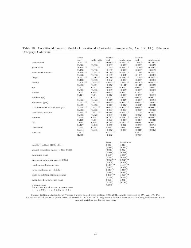
Table 18: Conditional Logistic Model of Locational Choice–Full Sample (CA, AZ, TX, FL), ReferenceCategory: California

Texas Florida Arizonacoef odds ratio coef odds ratio coef odds ratio

naturalized -3.761*** 0.023*** -0.982*** 0.374*** -1.960*** 0.141***(0.328) (0.008) (0.088) (0.033) (0.250) (0.035)

green card -3.859*** 0.021*** -1.304*** 0.271*** -1.525*** 0.218***(0.150) (0.003) (0.106) (0.029) (0.069) (0.015)

other work author. -3.366*** 0.035*** -0.797*** 0.451*** -1.154*** 0.315***(0.223) (0.008) (0.136) (0.061) (0.113) (0.036)

illegal -4.132*** 0.016*** -0.738*** 0.478*** -1.406*** 0.245***(0.103) (0.002) (0.082) (0.039) (0.036) (0.009)

female -0.308*** 0.735*** 0.429*** 1.535*** -0.440*** 0.644***(0.083) (0.061) (0.072) (0.111) (0.147) (0.095)

age 0.007 1.007 -0.007 0.993 0.027*** 1.027***(0.005) (0.005) (0.005) (0.005) (0.003) (0.003)

spouse 0.178 1.195 -0.079* 0.924* 0.112 1.119(0.121) (0.144) (0.042) (0.039) (0.076) (0.086)

children (#) 0.011 1.011 0.004 1.004 -0.016 0.984(0.026) (0.026) (0.015) (0.015) (0.020) (0.020)

education (yrs) -0.093*** 0.911*** -0.079*** 0.924*** 0.011*** 1.011***(0.019) (0.018) (0.013) (0.012) (0.001) (0.001)

U.S. farmwork experience (yrs) -0.029*** 0.972*** -0.010*** 0.990*** -0.020*** 0.981***(0.003) (0.003) (0.004) (0.004) (0.004) (0.004)

used work network -0.234*** 0.791*** -0.523*** 0.593*** -1.377*** 0.252***(0.033) (0.026) (0.063) (0.037) (0.092) (0.023)

summer 0.219* 1.244* -0.760*** 0.468*** -0.450*** 0.638***(0.129) (0.161) (0.027) (0.013) (0.049) (0.031)

fall 0.146 1.158 -0.729*** 0.482*** -0.081 0.922(0.127) (0.146) (0.056) (0.027) (0.076) (0.070)

time trend 0.018 1.018 0.029 1.029 0.021 1.021(0.044) (0.045) (0.052) (0.054) (0.041) (0.042)

constant 2.387* 9.167*** 2.275**(1.369) (2.432) (0.936)

State Attributesmonthly welfare (100s USD) 0.017 1.017

(0.015) (0.015)annual education value (1,000s USD) -0.029 0.972

(0.018) (0.018)minimum wage 0.506* 1.659*

(0.272) (0.451)linewatch hours per mile (1,000s) -0.050*** 0.951***

(0.008) (0.008)rural unemployment rate 0.143*** 1.154***

(0.053) (0.061)farm employment (10,000s) 0.043** 1.043**

(0.021) (0.022)state population Hispanic share 0.487*** 1.627***

(0.138) (0.224)mean hired farmworker wage 0.068 1.071

(0.177) (0.189)Observations 76308Robust standard errors in parentheses∗ ∗ ∗p < 0.01, ∗ ∗ p < 0.05, ∗p < 0.1

Source: National Agricultural Workers Survey, pooled cross sections 1989-2004, sample restricted to CA, AZ, TX, FL.Robust standard errors in parentheses, clustered at the state level. Regressions include Mexican state of origin dummies. Labor

market variables are lagged one year.

39

welfare and education program generosity is not an important determinant of locational choice for workers in

the border states.34 This is consistent with the empirical evidence in Section 5 and provides further evidence

for a lack of welfare migration by agricultural workers to these areas.35 This study finds strong, positive,

rural unemployment rate and farm employment effects. All else equal, migrants are 15.4 percent more likely

to choose a state with a one percent higher unemployment rate and 4.3 percent more likely to choose a state

with 10,000 more people in the farm workforce. Previous studies (e.g. Buckley (1996), Zavodny (1997)) find

similar positive correlations between unemployment rates and migration choices. Dodson (2001) hypothesizes

that either the time lag on the unemployment variable used in these studies is inappropriate, or that if all U.S.

state-level unemployment rates are of much lower magnitude than unemployment rates in origin countries,

differentials between states may not be relevant in locational decision-making. It is unclear whether this

argument should hold in this case given that the majority of NAWS workers are from Mexico. Official

Mexican unemployment rates are generally much lower than U.S. rates, but the accountability of these rates

is controversial. The labor market variables in the model (rural unemployment rate, farm employment,

and mean hired farmworker wage) are included as one-year lags. Including these variables at their current

levels or at two-year lags (not shown) leads to similar results, as does using statewide unemployment rates

in current or lagged form instead of rural rates. Labor market variables such as rural unemployment rates

represent general equilibrium outcomes. Therefore, the nonintuitive positive coefficient associated with the

rural unemployment rate should not be interpreted only in light of farm labor supply. The supply and

demand factors driving the sign and magnitude of this coefficient are not separately identified here.

Differences in minimum wages and the Hispanic percentage of the population are positive determinants

of locational choice within the border states. Migrants are 65.9 percent more likely to choose regions with a

dollar higher minimum wage. This suggests that minimum wages may be a more relevant policy instrument

related to migrant flows than are welfare and education program values as measured here. A strong positive

effect is also noted for state population Hispanic share. The odds ratio for state population percent Hispanic

indicates that migrants are 62.7 percent times more likely to choose a state with a one percent higher His-

panic share. A strong negative effect is noted for linewatch hours per mile. Migrants are almost five percent

less likely to choose a state with 1,000 more linewatch hours per mile than a state with less rigid border

enforcement all else equal.36 Gathmann (2004) and Angelucci (2005) argue that there is an endogenous

relationship between migrant flows and border enforcement. These authors instrument for border enforce-34The implicit assumption here is that education expenditure and quality are positively correlated (or at least expected

to be positively correlated by migrants). Continuing work examines additional characteristics of education programs such asstandardized test scores that may be more directly related to educational outcomes.

35Pena (2007) finds that Central American migrants are sensitive to welfare and education values while Mexican migrantsare not.

36Boeri, Hanson, and McCormick (2002) document that non-border patrol apprehensions are low in comparison with borderapprehensions. Florida border patrol values are approximated using Texas values.

40

ment with Drug Enforcement Administration budgets. Gathmann (2004) finds that enforcement has shifted

illegal migrant flows to more remote crossing places. The results of this paper are consistent with her story.

Angelucci (2005) finds that the overall effect of enforcement on total illegal migrant flows is ambiguous after

instrumentation. Adding instrumental variables to the conditional logistic framework is an area warranting

further econometric research.

7.4 Note Regarding Independence of Irrelevant Alternatives

Conditional logistic regression imposes an Independence of Irrelevant Alternatives (IIA) assumption. This

imposition may not be desirable. Regressions under different assumptions of the state options set S yield

similar results. These results are reported and further discussed in Pena (2007).

8 Conclusions

This paper examines whether individual states are welfare magnets for immigrants in various legal status

groups. Previous studies of welfare migration have excluded illegal immigrants, yet legislation suggests that

welfare migration by this population is of concern to individual states within the U.S. A focus of this paper is

to extend the literature to this group. While there is strong evidence that illegal immigrants cluster in certain

states, particularly those of the border, this study does not find that these patterns are systematically related

to state welfare generosity. The locational clustering behavior that is evident among the illegal population

is more the result of labor market conditions, network effects, and border enforcement than the result of

the availability or generosity of welfare benefits at the state level. Still, this paper finds that the result

of Borjas (1999) that legal immigrants who participate in welfare programs are geographically clustered in

California continues to hold using the most recent U.S. Census data. These data correspond to four years

after PRWORA. This result, however, does not hold for those in agriculture, a traditionally low skilled

occupation and frequent employer of illegal workers. Because much of the empirical analysis is descriptive,

this paper only begins to characterize the relationship between public economic activity (provision of goods

and services, transfers, and taxes) at state and local levels and immigrant geographical decisions.

41

References

Ai, C., and E. C. Norton (2003): “Interaction Terms in Logit and Probit Models,” Economics Letters,

80, 123–129.

Angelucci, M. (2005): “U.S. Border Enforcement and the Net Flow of Mexican Illegal Migration,” Dis-

cussion Paper 1642, IZA.

Bartel, A. P. (1989): “Where Do the New U.S. Immigrants Live?,” 7(4), 371–391.

Berry, W. D., R. C. Fording, and R. L. Hanson (2000): “An Annual Cost of Living Index for the

American States, 1960-2000,” Journal of Politics, 60(2), 550–567.

(2003): “Cost of Living Index for the United States, 1960-2000,” Computer File, Inter-University

Consortium for Political and Social Research, Ann Arbor.

Boeri, T., G. Hanson, and B. McCormick (eds.) (2002): Immigration Policy and the Welfare System.

Oxford University Press, Oxford.

Borjas, G. J. (1999): “Immigration and Welfare Magnets,” Journal of Labor Economics, 17(4.1), 607–637.

Borjas, G. J., S. G. Bronars, and S. J. Trejo (1992): “Self-Selection and Internal Migration in the

United States,” Journal of Urban Economics, 32, 159–185.

Boskin, M. J. (1974): “A Conditional Logit Model of Occupational Choice,” The Journal of Political

Economy, 82(2), 389–398.

Buckley, F. (1996): “The Political Economy of Immigration Policies,” International Review of Law and

Economics, 16, 81–99.

Camarota, S. A. (2004): “The High Cost of Cheap Labor: Illegal Immigration and the Federal Budget,”

Discussion Paper 23, Center for Immigration Studies.

Chiquiar, D., and G. H. Hanson (2005): “International Migration, Self-Selection, and the Distribution

of Wages: Evidence from Mexico and the United States,” Journal of Political Economy, 113(2), 239–281.

Davenport, P. (2006): “Workers’ Comp Benefits at Issue: Entrant’s Claim to Disability Pay Sparks

Questions,” Arizona Daily Star.

Dodson III, M. E. (2001): “Welfare Generosity and Location Choices among New United States Immi-

grants,” International Review of Law and Economics, 21, 47–67.

42

Flores, E. T. (1984): “Research on Undocumented Immigrants and Public Policy: A Study of the Texas

School Case,” International Migration Review, 18(3), 505–523.

Gabbard, S. M., R. Mines, and J. M. Perloff (1991): “A Comparison of the CPS and NAWS Surveys of

Agricultural Workers,” Discussion paper, Institute of Industrial Relations Working Paper Series, University

of California, Berkeley.

Gathmann, C. (2004): “The Effects of Enforcement on Illegal Markets: Evidence from Migrant Smuggling

along the Southwestern Border,” Stanford Center for International Development Working Paper No. 227.

Jaeger, D. A. (2000): “Local Labor Markets, Admission Categories, and Immigrant Location Choice,”

Discussion paper.

Kaushal, N. (2005): “New Immigrants’ Location Choices: Magnets without Welfare,” Journal of Labor

Economics, 23(1), 59–80.

Levinson, D. R. (2005): “Self-Declaration of U.S. Citizenship for Medicaid,” Department of Health and

Human Services, Office of Inspector General, Report OEI-02-03-00190.

Martin, P. L. (1996): Promises to Keep: Collective Bargaining in California Agriculture. Iowa State

University Press, Ames, Iowa.

McFadden, D. (1974): “Conditional Logit Analysis of Qualitative Choice Behavior,” in Frontiers in Econo-

metrics, ed. by P. Zarembka, pp. 105–142. Academic Press, New York.

Moretti, E., and J. M. Perloff (2000): “Use of Public Transfer Programs and Private Aid by Farm

Workers,” Industrial Relations, 39, 26–47.

Orrenius, P. M., and M. Zavodny (2005): “Self-Selection among Undocumented Immigrants from Mex-

ico,” Journal of Development Economics, 78, 215–240.

Passel, J. S. (2006a): “Estimates of the Unauthorized Migrant Population for States based on the March

2005 CPS,” Discussion paper, Pew Hispanic Center.

(2006b): “The Size and Characteristics of the Unauthorized Migrant Population in the U.S.:

Estimates Based on the March 2005 Current Population Survey,” Discussion paper, Pew Hispanic Center.

Pena, A. A. (2007): “Locational Choices of the Legal and Illegal: Mexican Agricultural Workers in the

U.S.,” Discussion paper.

43

Tiebout, C. M. (1956): “A Pure Theory of Local Expenditures,” The Journal of Political Economy, 64(5),

416–424.

Zavodny, M. (1997): “Welfare and the Locational Choices of New Immigrants,” Federal Reserve Bank of

Dallas, Economic Review, pp. 2–10.

(1999): “Determinants of Recent Immigrants’ Locational Choices,” International Migration Review,

33(4), 1014–1030.

44

A Data Appendix

A.1 NAWS Sampling Methodology

The sampling procedure of the National Agricultural Workers Survey is based on four levels: region, crop

reporting district, county, and employer with probabilities proportional to size at each level. Specifically,

NAWS uses 12 geographic regions based on USDA Quarterly Agricultural Labor Survey of farm employers.

The 12 regions are defined in Table 1 earlier in the paper. USDA information is also used for cyclical allocation

(based on the relative proportions of workers each cycle). There are 47 Crop Reporting Districts (aggregates

of counties with similar agricultural characteristics) from which sampling locations are selected. Within Crop

Reporting District, counties are selected randomly without replacement with probabilities proportional to the

county’s farm labor expenses. Employer lists are from the Bureau of Labor Statistics Agricultural Soil and

Conservation Service and are updated with information from county extension agencies, local employment

agencies, grower organizations, and farmworker service programs. Employers are selected using probabilities

proportional to the square root of the seasonal farm workforce. Once permission to interview is obtained, the

maximum number of interviews per grower is determined with probabilities proportional to square root size.

The number of interviews per site of a particular grower is also determined by a proportional distribution

to total number of crop workers at each work site. Workers are selected and approached randomly when

arriving for work, at lunch, or when leaving and interviews are scheduled for convenient times away from

work site at locations chosen by the workers.

A.2 Supplementary State Policy, Labor Market, and Demographic Data

State policy variables include welfare values, education expenditure, minimum wages, and border patrol

intensity. Maximum monthly AFDC/TANF benefit levels and FSP values are from the U.S. House of

Representatives Committee of Ways and Means. Figure A-1 presents the case of a family of four. Values of

these variables for other family structures are parallel shifts up or down of these curves for each state. Welfare

data for 1995, 1997, 1999, 2002, and 2003 were imputed linearly, as these data are otherwise unavailable.

Figure A-2 presents the welfare data for a family of four in real terms. The series is deflated by a state-level

cost of living deflator, the CPI2000, developed by Berry, Fording, and Hanson (2003). Values are in year

2000 dollars based on the median cost of living state in 2000. The two middle states in terms of cost of living

in that year, South Dakota and Delaware, were averaged and serve as the base for the index.

Data on current expenditure per pupil in public elementary and secondary schools in Figure A-3 are

from the U.S. Department of Education, Digest of Education Statistics and from the National Education

45

Association, Rankings and Estimates. As the value of the welfare and education variables to the individual

migrant varies with his or her family size, these variables are matched to respondents based on reported

family characteristics.

Minimum wage data are from the Department of Labor and are presented in Figure A-4. Arizona, Texas,

and Florida did not have state-level minimum wages in place during the time period corresponding to NAWS

data. Federal minimum wage rates are used for these states.

Border Patrol linewatch hours per mile, in Figure A-5, are from unpublished INS/Homeland Security data

shared by Gordon H. Hanson and Christina Gathmann. The Department of Homeland Security (formerly

the INS) divides the U.S.-Mexico border into nine sectors: San Diego and El Centro in California, Yuma

and Tucson in Arizona, and El Paso, Marfa, Del Rio, Laredo, and McAllen in Texas. Linewatch hours are

adjusted for border mile coverage and averaged by state, where state is defined as that state housing the

sector’s central city.

State labor market and demographic variables include rural unemployment rates, farm employment,

Hispanic share of the state’s population, and average wage rates. Rural unemployment rates are calculated

using inputs from Economic Research Service of USDA. Rates are based on 2003 non-metro classifications.

The 2003 rural classifications should represent the most rural areas, as these areas have remained in the

rural classification over time. Rural unemployment rates based on 1983 and 1993 classifications were also

calculated and are available from the author. Figure A-6 shows these rates over time.

Farm employment, presented in Figure A-7, are from Economic Research Service of USDA and the Bureau

of Economic Analysis of the Department of Commerce. California employment totals are presented on the

left hand side axis, while data for the other states follow the right axis.

Hispanic share of state’s population is from the U.S. Census (Figure A-8). Data for year 2000 on include

those classifying themselves as “Latino.” This difference in definition drives the nonlinearity in the data in

year 2000.

Annual average wage rates of hired field workers are from USDA (Figure A-9). The wages reported for

Arizona and Texas in the 1989-1991 period are averages of wages in the USDA agricultural regions including

these states. Data for later years correspond to average wages specific to those states.

46

Fig

ure

A-1

:(N

omin

al)

Max

imum

Mon

thly

AFD

C/T

AN

Fpl

usFSP

Ben

efits

for

aFa

mily

ofFo

ur

0

200

400

600

800

1000

1200

1400

1989

1990

1991

1992

1993

1994

1995

1996

1997

1998

1999

2000

2001

2002

2003

2004

dollars per month

CA

AZ

TXFL

Sour

ce:

U.S

.H

ouse

ofR

epre

sent

ativ

esC

omm

itte

eof

Way

san

dM

eans

,Gre

enB

ook,

sele

cted

year

s

47

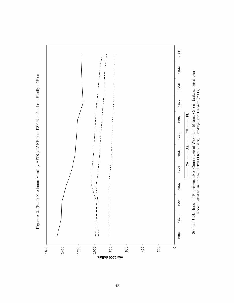
Fig

ure

A-2

:(R

eal)

Max

imum

Mon

thly

AFD

C/T

AN

Fpl

usFSP

Ben

efits

for

aFa

mily

ofFo

ur

0

200

400

600

800

1000

1200

1400

1600

1989

1990

1991

1992

1993

1994

1995

1996

1997

1998

1999

2000

year 2000 dollars

CA

AZ

TXFL

Sour

ce:

U.S

.H

ouse

ofR

epre

sent

ativ

esC

omm

itte

eof

Way

san

dM

eans

,Gre

enB

ook,

sele

cted

year

sN

ote:

Defl

ated

usin

gth

eC

PI2

000

from

Ber

ry,F

ordi

ng,a

ndH

anso

n(2

003)

48

Fig

ure

A-3

:(N

omin

al)

Cur

rent

Exp

endi

ture

inP

ublic

Ele

men

tary

and

Seco

ndar

ySc

hool

s

0

1000

2000

3000

4000

5000

6000

7000

8000

9000

1989

1990

1991

1992

1993

1994

1995

1996

1997

1998

1999

2000

2001

2002

2003

2004

2005

annual dollars per pupil in average daily attendance

CA

AZ

TXFL

Sour

ces:

U.S

.Dep

artm

ent

ofE

duca

tion

,Dig

est

ofE

duca

tion

Stat

istics

,sel

ecte

dye

ars

and

Nat

iona

lEdu

cation

Ass

ocia

tion

,Ran

king

san

dE

stim

ates

,se

lect

edye

ars

49

Fig

ure

A-4

:(N

omin

al)

Fede

ralv

ersu

sSt

ate

Min

imum

Wag

es

012345678

1989

1990

1991

1992

1993

1994

1995

1996

1997

1998

1999

2000

2001

2002

2003

2004

dollars per hour

CA

Fede

ral

Sour

ce:

Dep

artm

ent

ofLab

or

50

Fig

ure

A-5

:B

orde

rPat

rolL

inew

atch

Hou

rspe

rM

ile

0510152025

1989

1990

1991

1992

1993

1994

1995

1996

1997

1998

1999

2000

2001

2002

2003

2004

person hours (in 1000s)

CA

AZ

TX

Sour

ce:

INS/

Hom

elan

dSe

curi

tyvi

aG

ordo

nH

anso

nan

dC

hris

tina

Gat

hman

n

51

Fig

ure

A-6

:R

ural

Une

mpl

oym

ent

Rat

es

02468101214

1989

1990

1991

1992

1993

1994

1995

1996

1997

1998

1999

2000

2001

2002

2003

2004

2005

percent

CA

AZ

TXFL

Sour

ces:

Eco

nom

icR

esea

rch

Serv

ice,

USD

Aan

dau

thor

’sca

lcul

atio

nsN

ote:

base

don

2003

Met

ro/N

onm

etro

clas

sific

atio

ns

52

Fig

ure

A-7

:Fa

rmW

age

and

Sala

ryW

orke

rsE

mpl

oym

ent

050100

150

200

250

300

1989

1990

1991

1992

1993

1994

1995

1996

1997

1998

1999

2000

2001

2002

2003

2004

CA employment (in 1000s)

010203040506070

AZ, TX, FL employment (in 1000s)

CA

AZ

TXFL

Sour

ces:

Eco

nom

icR

esea

rch

Serv

ice,

USD

Aan

dB

urea

uof

Eco

nom

icA

naly

sis,

Dep

artm

ent

ofC

omm

erce

53

Fig

ure

A-8

:H

ispa

nic

Shar

eof

Stat

e’s

Pop

ulat

ion

0510152025303540

1990

1991

1992

1993

1994

1995

1996

1997

1998

1999

2000

2001

2002

2003

2004

percent

CA

AZ

TXFL

Sour

ce:

U.S

.C

ensu

sB

urea

u

54

Fig

ure

A-9

:(N

omin

al)

Ann

ualA

vera

geW

age

Rat

esof

Hir

edFie

ldW

orke

rs

012345678910

1989

1990

1991

1992

1993

1994

1995

1996

1997

1998

1999

2000

2001

2002

2003

2004

2005

dollars per hour

CA

AZ

TXFL

Sour

ce:

USD

AN

ote:

1989

-199

1“A

Z”

and

“TX

”w

ages

base

don

USD

Aag

ricu

ltur

alre

gion

s

55

Immigration, Legal Status, and Public Aid Magnets

Documents

Transcript of Immigration, Legal Status, and Public Aid Magnets