IZA DP No. 3217

Immigrant Networks and Their Implications forOccupational Choice and Wages

Krishna PatelFrancis Vella

DI

SC

US

SI

ON

PA

PE

R S

ER

IE

S

Forschungsinstitutzur Zukunft der ArbeitInstitute for the Studyof Labor

December 2007

Immigrant Networks and Their Implications for Occupational

Choice and Wages

Krishna Patel Georgetown University

Francis Vella

Georgetown University and IZA

Discussion Paper No. 3217 December 2007

IZA

P.O. Box 7240 53072 Bonn

Germany

Phone: +49-228-3894-0 Fax: +49-228-3894-180

E-mail: iza@iza.org

Any opinions expressed here are those of the author(s) and not those of the institute. Research disseminated by IZA may include views on policy, but the institute itself takes no institutional policy positions. The Institute for the Study of Labor (IZA) in Bonn is a local and virtual international research center and a place of communication between science, politics and business. IZA is an independent nonprofit company supported by Deutsche Post World Net. The center is associated with the University of Bonn and offers a stimulating research environment through its research networks, research support, and visitors and doctoral programs. IZA engages in (i) original and internationally competitive research in all fields of labor economics, (ii) development of policy concepts, and (iii) dissemination of research results and concepts to the interested public. IZA Discussion Papers often represent preliminary work and are circulated to encourage discussion. Citation of such a paper should account for its provisional character. A revised version may be available directly from the author.

IZA Discussion Paper No. 3217 December 2007

ABSTRACT

Immigrant Networks and Their Implications for Occupational Choice and Wages*

This paper employs United States Census data to study the occupational allocation of immigrants. The data reveal that the occupational shares of various ethnic groups have grown drastically in regional labor markets over the period 1980 to 2000. We examine the extent to which this growth can be attributed to network effects. That is, we examine the relationship between the occupational choice decision of recently arrived immigrants with those of established immigrants from the same country. We also consider the earnings implications of these immigrant networks for recent arrivals. The empirical evidence strongly suggests the operation of networks in the immigrant labor market. First, we find evidence that new arrivals are locating in the same occupations as their countrymen. Moreover, this location decision is operating at the level of regional labor markets. Second, we find that individuals who locate in the "popular" occupations of their countrymen enjoy a large and positive effect on their hourly wage and their level of weekly earnings. JEL Classification: J24, J3, J61 Keywords: network effects, immigrants, occupational choice, earnings Corresponding author: Francis Vella Department of Economics Georgetown University Washington, DC 20057 USA E-mail: fgv@georgetown.edu

* We are grateful to Jim Albrecht and Pieter Gautier for helpful comments.

1 Introduction

In 1980 0.68% of all hairdressers and cosmetologists in the Houston-Brazoria metropolitan area

were born in Vietnam. By 1990 this percentage had grown to 6.21% and by 2000 it was 24.18%. In

Fort Lauderdale, 4.00% of food preparation workers in 1980 were from Haiti. This share increased

to 23.52% in 1990 and to 26.56% in 2000. While each of these trends is remarkable they are

not atypical. An examination of the occupational allocation decisions of immigrant workers in

metropolitan areas suggests that all across the United States, immigrants from a range of countries

have developed local niches in specific occupations.

If such a phenomena is occurring on a larger scale, and this is one question we address here, it

is useful to consider potential explanations of this remarkable occupational concentration. First,

the 1965 amendment to the US Immigration Act eliminated country specific quotas and produced

a large increase in the number of immigrants.1 This increase would explain a general growth in

their share of some occupations providing that; i) the native born population did not increase at

the same rate; and/or ii) the new immigrants were not allocated across occupations in a manner

which preserved the previous allocation. A second explanation is related to the skill portfolios that

accompany immigrants. If there was a drastic increase in the number of migrants from a particular

country and these migrants all had a specific skill(s), it is likely that their share of occupations that

require that skill would increase accordingly (see, for example, Roy 1951). Third, it is possible that

local labor markets are experiencing occupation specific shocks and this is generating increased

labor demand in these occupations. If immigrants are more mobile than natives it is likely they

will locate in these newly created positions (see Borjas 2001).

While each of the above would appear to at least partially contribute to the observed trends

in occupational concentration by immigrants the drastic trends noted above, and many others we

detail below, seems suggestive of an additional process. That is, the growth of the number of

immigrants from various countries in a range of occupations suggests that new immigrants are

following their countrymen and finding employment in the same occupations. We interpret this

occupational location decision as the product of a network effect. Establishing the presence of such

1The country specific quotas were replaced with a world-wide limit on immigrants. In 1996 the visa limit was507,000, of which 62% were for family reunification. Immediate family of US citizens are exempt from immigrationquotas and in the mid 1990s over 70% of immigrants came under family reunification (Borjas 1999).

2

an effect is an important exercise as it has obvious welfare implications for immigrants if it leads

to employment opportunities. Network effects would be even more economically significant if they

had implications for wages and earning levels.

In this paper we attempt to identify and estimate the magnitude of one specific form of im-

migrant network effects on the occupational allocation of immigrants using United States Census

data for the years 1980, 1990 and 2000. More explicitly we examine if the occupational choices of

recently arrived immigrants are influenced by the occupational location of their predecessors. We

also investigate the empirical implications of these networks for the wages and weekly earnings of

recent immigrants. In the following section we discuss the literature relevant to network effects

and occupational choice. Section 3 provides a simple labor market search model which incorpo-

rates a role for immigrant networks. Section 4 discusses our data and sample selection. Section

5 documents the trends in occupational shares by immigrant groups in local labor markets while

Section 6 reports the estimates from a model which explains the probability that a recently ar-

rived immigrant will choose the occupation most commonly adopted by previous immigrants from

his/her country. Section 7 explores whether there are any wage and earnings implications from this

location decision. Section 8 provides a more detailed discussion of our empirical results. Section 9

provides some concluding comments.

2 Literature

In reviewing the literature related to the role of networks in the occupational choice decision

it is useful to begin with our use of the term "network" and the precise effect we seek to uncover

in our empirical investigation. We assume that individuals that come from the same country and

who are located in the same metropolitan area are likely to have a relatively higher propensity to

interact. This may reflect common acquaintances in the US or their home country, or their common

cultural background. We now briefly examine the existing literature, both theoretical and empirical,

which explains how this type of network membership might influence an individual’s propensity to

take employment in the same occupation as the other network members. These effects are likely

to operate through an individual’s employment search method and also the level of potential job

offers. It is also a way of acquiring job offers (see, for example, Montgomery 1991). For employers

3

these networks may represent a mechanism for screening potential workers.

Previous empirical evidence has established that networks are important in influencing individ-

ual employment outcomes. For example, 17% of those unemployed workers surveyed in the 1970

Current Population Survey (CPS) consulted friends and relatives for work. This figure grew to 23%

in the 1991 CPS (Bradshaw 1973, Bortnick and Ports 1992, Ioannides and Datcher Loury 2004).

Networks are useful for both employed and unemployed workers both in terms of frequency of job

offers and acceptance (Blau and Robins 1990, Blau 1992). Over a range of data sets it was found

that between 30 to 60 percent of job matches were made through personal ties, with a greater

prevalence of network use among low skilled workers (Ioannides and Datcher Loury 2004).

Several theoretical studies investigate the impact of the dissemination of information through

networks on job search. While job information acquired through networks generally improves both

the individual’s probability of employment and wage level there are circumstances under which they

might both decline (Calvo Armengol and Jackson 2003, 2004). The empirical evidence, however,

generally suggest that networks improve the probability of employment of its members (see Munshi

2003, Beaman 2007, Laschever 2007). The evidence further suggests that a network defined by

geographic proximity has a positive influence on individual employment. These neighborhood

effects tend to be particularly strong between ethnically similar locations (see Bayer et al 2004,

Topa 2001, Laschever 2007). For example, Edin et al (2003) show a large and positive income effect

for immigrant refugees living in ethnic enclaves in Sweden.

The empirical economics literature on networks in the labor market has focused either on un-

employment or wages while largely ignoring occupational choice. The sociology literature, however,

discusses the importance of immigrant networks in developing occupation niches. These studies are

generally historical in nature and suggest that immigrant groups which shared employment opportu-

nities through their networks perform better in terms of obtaining employment in higher paid occu-

pations (Model 1993). Waldinger (1996) suggests that the rapid movement of white native workers

away from certain jobs in New York city enabled ethnic minorities to form niches. Networks then

channeled immigrants of specific ethnic backgrounds into specific occupations. Waldinger (1994)

studied immigrant workers in New York City’s government, a sector in which immigrants started

to emerge more prominently during the latter part of the twentieth century, and finds that immi-

grants sorted into different occupations within city government according to ethnic background.

4

Some empirical studies, (see, for example, Logan, Alba and Zhang 2002), suggest that immigrants

choose their occupation after choosing their location. Since a majority of immigrants are based

on family re-unification their location decisions, and subsequently their occupational choices, are

constrained (Parks 2005).

One economic investigation of interest is Munshi and Wilson (2007) which explores the influence

of the occupational choice of nineteenth century immigrants on those of current immigrants from

the same country. The focus of that paper is on cultural identity defined by the occupation choice of

the first generation of immigrants. The empirical component of the paper focuses on the probability

of accepting a high skilled job over a low skilled job.

3 Conceptual Framework

To motivate the empirical work that follows we present a simple model of the search behavior

of immigrants. The unemployed are able to search for a job and this may take place through formal

channels such as newspaper advertisements or online postings. Alternatively, the search may occur

through informal channels. We define the informal channel as the individual’s network of employed

friends and relatives.

Let S denote the set of occupations for which individual i is qualified. Let SN denote the set

of occupations included in his network for which the individual is qualified. Therefore, SN ⊂ S.

Assume a continuous time model in which job offers follow a Poisson process and can arrive from

either channel. Jobs offers in occupation o arrive via the formal channel with arrival rate po, while

they arrive in occupation o via the network at rate pNo .

We assume that recently arrived immigrants seek to maximize the expected value of discounted

future income using discount rate r. While unemployed the individual receives b through unem-

ployment compensation or leisure. Since there is a distribution of wages offered in occupation o,

the individual does not know the actual wage offered ex-ante. Let wo represent the wage offered

through the formal channel in occupation o with distribution Fo(wo), and wNo represent the wage

offered in occupation o through the network channel with distribution FNo (wNo ). When employed

in occupation o the individual receives wage wo, or alternatively wNo , forever. The value of working

in a job found through the formal channel and the informal channel can be defined, respectively,

5

as W (wo) =wor

and W (wNo ) =wNor. The value of being unemployed can thus be expressed as:

rU = b+∑

o∈S

po

∫max[W (wo)− U, 0]dFo(wo) +

∑

o∈SN

pNo

∫max[W (wNo )− U, 0]dF

No (w

No ). (1)

The first term in this expression represents the flow value of unemployment. The second and

third terms capture the expected values from being employed when the job offer arrives from the

formal and network channels respectively, noting that the expectation is taken over the wages

offered in occupation o through each channel. Once the individual encounters a job with wage

realization wo (or wNo ), he/she would accept a job offer if W (wo) (or W (w

No )) is greater than U .

The arrival rate of a job offer in occupation o from the network channel is directly proportional to

the number of people in the network who are employed in occupation o. Assume no represents the

number of people in the individual’s network who are employed in occupation o and all individuals

in the network face the same arrival rate po. Then pNo can be expressed as:

pNo =∑

i∈no

pio = nopo. (2)

When confronted with a job offer in occupation o, the individual will accept the offer provided

the offered wage, wo, is at least as large as his/her reservation wage. The reservation wage is the wage

that makes the individual indifferent between being employed and being unemployed and solves

W (wR) = U . Rearranging, and noting that W (wo) =wor, implies rU = wR and W − U = w−wR

r.

Inserting this into equation (1) and simplifying gives the following expression for the reservation

wage:

wR = b+∑

o∈S

po

∫

wR

wo −wR

rdFo(wo) +

∑

o∈SN

pNo

∫

wR

wNo −wR

rdFNo (w

No ). (3)

Simplifying (3) further gives

wR = b+1

r

∑

o∈S

po

∫

wR

[1− Fo(wo)]dwo +1

r

∑

o∈SN

pNo

∫

wR

[1− FNo (wNo )]dw

No . (4)

Using equations (2) and (4) the following results can be obtained. First, since the overall arrival

6

rate of a job in occupation o can be expressed as Po = po + pNo , then

∂Po∂no

= po > 0. That is, the

overall arrival rate of a job in occupation o increases in the number of people in the network who

are employed in occupation o.

Second, applying the implicit function theorem to (4) suggests that the reservation wage is

increasing in the number of people in the network employed in occupation o, ∂wR∂no

> 0. To see this,

note that the reservation wage is increasing in the arrival rate of job offers, a result that is standard

in search models. Since the arrival rate of job offers in occupation o is increasing in the network

size in occupation o, no, the reservation wage is also increasing in no. Intuitively, if individuals

encounter more job offers, they become more selective about the jobs they will accept. We would

expect individuals with a higher reservation wage to accept higher wage jobs on average.

Furthermore, “clustering” in occupation o would arise when acceptable offers in occupation o

arrive from the network channel at a faster rate than acceptable job offers in any other occupation

that arrive through the formal channel. That is, when pNo Pr(wNo > wR) >

∑k∈S pk Pr(wk > wR).

This occurs when either no is large or when Pr(wNo > wR) > Pr(wk > wR), ∀k �= o or both.

While the above model is simple and is presented primarily to motivate our examination of

the data, it provides two clear predictions. First, the probability an individual will locate in an

occupation is a function of the size of the individual’s network in that occupation. Second, the

individual’s reservation wage, and by implication the accepted wage, is positively related to the

size of the individual’s network in the occupation.

4 Data and Key Variable Definitions

To examine the growth in occupational shares we employ the five percent samples from the 1980,

1990 and 2000 US Censuses. While the census is only available at ten year intervals, it provides

a sufficiently large number of observations to identify occupational growth patterns in the various

regions comprising the US. The occupation codes used are based on the variable “occ1990” which

characterizes the individual’s occupation at the three digit level.2 This variable has approximately

300 classifications, based on the 1990 occupation classification scheme, and is comparable across

the years we consider.

2This measure is preferable to the occ1950 variable, also available for each of the years we consider, as it providesa more recent occupation classification scheme.

7

In our empirical analysis we distinguish between ‘new’ immigrants and ‘established’ immigrants

as we focus on the empirical relationship between the occupational choices of these two groups. For

this purpose, it would be most useful to observe the occupation of the immigrant’s first job entering

the US. However, such detailed work history variables are not available. The most recent immigrant

group which can be distinguished in the 1980 census are those individuals who have arrived in the

United States between 1975 and 1980. For the 1990 census, the most recent immigrants who can

be identified are those who immigrated in 1987. For the 2000 census, the most recent identifiable

immigrants are those arriving after 1998. To retain consistency across samples we define those

individuals who arrived in the US within five years of the survey date to be ‘new’ immigrants. All

remaining other foreign born workers, comprising those who have immigrated over five years prior

to the survey date, are considered ‘established’ immigrants. While this dichotomy is determined by

the limitations of the data it does not seem unreasonable. That is, determining what distinguishes

‘established’ from ‘new’ is arbitrary and the most important requirement is that one can identify

recent arrivals. In this sense the five year distinction does not seem unreasonable for our purposes.

To examine occupational growth by immigrant groups in local labor markets it is necessary to

have an operable definition of a local labor market. We define it to be a metropolitan area. There

are roughly 292 such areas identified in the census although the exact number varies by census

year. For the 2000 Census immigrant sample, 72,614 observations of 818,083 live in an unidentified

metropolitan area, compared to 124,291 observations that work in an unidentified metropolitan

area. We employ the metropolitan area of the workplace as our measure of where the individual is

located as this seems the better measure for our purposes.

As the data comprises a large number of occupations and an equally large number of metropol-

itan areas, and we also make a distinction within the immigrants on the basis of their country of

birth, small cell sizes are likely to be an issue. To describe the patterns in the data we initially

include observations for every metropolitan area which has at least 100 workers. However, we

subsequently focus our analysis on those immigrants who are employed in an identified occupation

in an identified metropolitan area where there at least 100 other immigrants from their country in

that metropolitan area. This selection criteria produces a very large data set, in terms of numbers

of individuals, and includes about 100 metropolitan areas and immigrants from approximately 100

countries working in over 250 occupations.

8

While our attention is initially on the occupational allocation of recent immigrants we subse-

quently focus on the impact of network membership on wages. This requires a measure of wages and

earnings. The census includes measures of annual wages, weeks worked and usual hours worked per

week for the previous calendar year. This allows the construction of an individual’s hourly wage.

This constructed hourly wage variable appears to be susceptible to measurement error at extreme

points in the distribution. For example, at the lower end, many hourly wages were calculated to

be less than 10 cents per hour while, at the upper end, there were many hourly wages that seemed

to be unreasonably high. Accordingly we trim the data by eliminating observations which are in

the top and bottom percentile. The descriptive statistics for our sample are provided in Appendix

Tables A4.1 and A4.2.

5 Occupation Shares by Country of Origin

To explore the growth in the occupational shares of ethnic groups in local labor markets Tables

5.1 and 5.2 report these shares for different origin countries at both the metropolitan and national

level. We reiterate that we only include occupations that had at least 100 observations in the

metropolitan area during at least one of the census years.

The first section of Table 5.1 presents the proportion of working individuals from country j in

area m in occupation o for each of the census years. The second section of the table reports the

proportion of those working in area m in occupation o who are from country j. It is these two

features of the data in which we are most interested. The first captures the tendency of individuals

from certain countries to go into specific occupations and reflects the network phenomenon which

is suggested by the conceptual model above. The second section reports the rate at which this

network effect is resulting in the domination of certain occupations in various regions by different

ethnic groups. The third section of the table reports the change over the three census years for the

estimates in the second section of the table. Table 5.1 also reports the country of origin population

as a percent of total population in the metropolitan area. Note that due to the extremely large

number of cells it is not possible to list each of them. Accordingly, for presentational purposes

we adopt the following strategy. For each country group in each area we tabulate the five most

popular occupations. This produces a list of 3,361 cells. We then rank these cells on the basis

9

of their growth in occupation share over the period 1980 to 2000 and list those at every second

percentile.3 For example, the first entry reports that Chinese textile workers who work in the New

York-Northeastern New Jersey metropolitan area had a change in occupation share at the 99-100

percentile. Their percentage share of that occupation in 1980 was 17.26 and this grew to 43.78 by

2000.

We acknowledge that Table 5.1 reports excessive information to be easily absorbed by the

reader. We present in its current form however, to illustrate the range of countries, metropolitan

areas and occupations which experience notable growth. The table also reveals that while the two

examples discussed in this paper’s opening paragraph are the most dramatic there are a number of

occupation/immigrant group cells which have seen extraordinary growth in certain areas. Moreover,

this growth is not limited to a small number of occupations. We pursue this below.

Table 5.2 provides the occupation shares for country groups that experienced the fastest growth

over 1980—2000. To illustrate that this phenomenon is not simply due to immigrants from Mexico,

who figure prominently in Table 5.1, we exclude them from this table. Table 5.2 suggests other

ethnic groups are also obtaining a growing share of certain occupations in local labor markets. It

appears the dramatic growth in occupation shares for these immigrant groups occurs primarily at a

metropolitan area level, as the corresponding occupation shares at the national level are relatively

modest and do not demonstrate clear patterns. Moreover, while many of these metropolitan areas

have a high proportion of immigrants, the growth in occupation share for the country groups is

disproportionate to its growth in population. Tables 5.1 and 5.2 suggest there is no clear rela-

tionship between metropolitan area population share and occupation share. A high share in a

particular occupation for a country group in one metropolitan area does not imply a high share in

the same occupation elsewhere. While this partially reflects regional variation in the distribution

of occupations it is interesting nevertheless. One particularly striking example, illustrated in Table

5.2, is that of textile sewing machine operators in New Bedford, MA. This metropolitan area has a

large but declining population of Portuguese workers which initially grew from 12.23% in 1980 to

17.82% in 1990 before decreasing to 10.22% in 2000. The proportion of Portuguese in this occupa-

tion grew steadily from 55.43% in 1980 to 69.42% in 1990 to 71.15% in 2000. It is also interesting

that the data indicates that this occupation is dominated by Chinese or Mexican workers in other

3Since there were multiple cells at each of the reported percentiles we chose one at random.

10

metropolitan areas. The fact that Chinese or Mexican workers in the textile occupation are prac-

tically absent in New Bedford, MA while Portuguese workers are absent in the textile occupations

in other metropolitan areas suggests that this observed specialization in local labor market is not

based on home country specific skills.

As the occupations which appear in these tables generally require a relatively low level of spe-

cialized training this might reflect that the strong presence of a country group in an occupation is

not the result of comparative advantage. To investigate this Table 5.3 presents for each country

of origin, the number of unique occupations that ranked as the most popular occupation across

metropolitan areas. The most popular occupation in a metropolitan area is defined to be the occu-

pation that has the highest fraction of that country’s members. For example, there were 18 distinct

most popular occupations for Puerto Rican workers across all metropolitan areas in the year 2000.

The first set of columns represent the number of unique occupations that were ranked the high-

est for each country group across all metropolitan areas. These numbers are somewhat misleading

because not every country group is represented in all metropolitan areas. Additionally, multiple

occupations were frequently tied for the top occupation rank in which case all tied-occupations

were counted. Therefore, the second set of columns represents a normalized measure of the dis-

tribution of top ranked occupations. It represents the number of unique occupations that are top

ranked across metropolitan areas divided by the number of metropolitan areas in which the coun-

try group is present. This number can exceed 1 when multiple occupations tie for the top rank.

Overall, a higher number suggests a higher dispersion of most popular occupation categories across

metropolitan areas. For most countries the occupation dispersion is well above 0.5 indicating there

is substantial variation in the preferred occupational location of each ethnic group.4 While this

variation may reflect "within" variation in the composition of immigrant groups across metropoli-

tan areas (i.e. people from the same country may select different metropolitan areas based on their

skill set), it is unlikely to explain why one low skilled occupation is popular among a country group

in one metropolitan area while another occupation is popular elsewhere. This table is important

for our purposes in that it suggests that the occupational choice of immigrants is not based on

comparative skill advantages.

One possible explanation for the patterns in Tables 5.1 and 5.2 is the presence of networks.

4The weighted average of this measure was approximately .3 for each of the Census years.

11

That is, new immigrants are locating in the sectors in which their countrymen are located. To

initially explore this Figures 1 to 3 plot for each metropolitan area, the fraction of immigrants who

have lived in the US for at least five years employed in each occupation against the fraction of new

immigrants (defined as those who have lived in the US for less than five years) employed in that

occupation. We do this for each of the census years noting that we plot the occupations that were

among the five most popular for established immigrants for each country group. The figures are

somewhat difficult to read due to the mass of points. However, the most simple interpretation is

that if recent immigrants located in occupations in the same proportions as their predecessors the

data points would be on the 45 degree line noting that the new migrants are on the vertical axis.

The figures reveal that for all three census years the majority of the data points are above the 45

degree line. This suggests that new immigrants are disproportionately following their predecessors.

While this is consistent with the presence of network effects it remains to condition out the other

factors which affect occupational location and we do this in the following section.

6 An Empirical Model of Immigrant Occupational Allocation

While Figures 1 to 3 are consistent with the operation of network effects, and the implications

of the conceptual model which predicts this type of relationship between the new and established

immigrants, the figures are also consistent with occupational specific growth by region. Accordingly

we now employ a more rigorous approach to identify the presence of network effects by estimating

an occupational choice model for recent immigrants.

To establish the underlying determinants of occupational location one could estimate a multino-

mial choice model where each of the occupations in the potential choice set represents a different

outcome. However, given that the important feature of the data that we report in the previous sec-

tion occurs at a relatively disaggregated level this would require estimating a discrete choice model

with an extremely large number of outcomes. This would not be feasible without the imposition

of a large number of unreasonable economic and statistical restrictions. Accordingly we focus on

one particular aspect of the occupational allocation decision of immigrants which is implied by our

conceptual model in Section 3. We examine whether a new arrival chooses the dominant occupation

for his/her immigrant group in the region in which he/she has arrived. That is, we estimate the

12

following:

Pr(Iijmot = 1) = α+ γ1Yestabjmot + γ2Ynmot + γ3Smot +Xitβ + ηijmot (5)

where Iijmot is an indicator function denoting that immigrant i from country j who locates in

metropolitan area m chooses occupation o in time period t. The choice of occupation depends

not only on the country from which the individual comes but reflects the most commonly chosen

occupation for that immigrant group in that metropolitan area prior to the arrival of the new

immigrants. The independent variable Y estabjmot measures the percent of people from country j working

in metropolitan area m of established immigrants who are in occupation o. This variable captures

our defined network effect and its coefficient γ1 is the object of primary interest. We also include

Ynmot which measures the proportion of people in that occupation o in metropolitan area m who

are native born. This variable captures the propensity of the occupation in that area to employ

immigrants (natives). To capture the relative size of the occupation we also include Smot which

denotes the proportion of workers in area m who are employed in occupation o in time t. We also

include a number of the individual’s characteristics, such as age, education, marital status, gender

and his/her capacity to speak english. In addition we include indicator functions for the individual’s

country of origin and the metropolitan area and region in which the individual works. These country

of origin variables are likely to capture any ethnic preference regarding occupation while the region

and metropolitan area dummies are included to capture unobserved demand effects. Finally, ηijmot

is assumed to be a zero mean error term.

An obvious objection to the OLS estimation of (5) is the endogeneity of the key regressor Y estabjmot .

It is possible that unobservable factors, such as labor demand shocks, simultaneously influence the

occupational choices of new and established immigrants. It is also possible, although less likely, that

the causality operates in the opposite direction. That is, the established workers may be relocating

depending on where the new arrivals find employment. The presence of unobservable factors and/or

reverse causality would bias our estimates. Accordingly we instrument Y estabjmot with Y estabjmot−10 which

denotes the occupational share of workers from country j in metropolitan aream in occupation o ten

years prior to the census for time t. This captures the occupational choices of an older generation of

immigrants that were made before the arrival of the new immigrants. These instruments are highly

correlated with the endogenous explanatory variables and have highly significant F statistics in the

13

corresponding first stage regressions.5 As the same objections may arise with respect to Ynmot and

Smot we use the same instrumenting strategy for these two variables.

We estimate the above model separately for the 1980, 1990 and 2000 census data. In each model

the unit of observation is the individual and the number of observations per cross section is shown

in Table 6.1. While the unit of observation is the individual for each cross section the variable

Y estabjmot shows variation by area, occupation and immigrant group while Ynmot and Smot vary by area

and occupation.

The dependent variable in equation (5) takes the value 1 if the individual is working in the most

popular occupation of the people from his/her country in the metropolitan area where he/she works.

Given the large number of occupations it is possible that there may be several "equally" popular

occupations for each immigrant group in each region. Accordingly, we re-estimate the model where

we define a series of dependent variables corresponding to the events that the individual selected

an occupation among the most popular two, the most popular three, the most popular four and

finally the most popular five. The independent variables are also redefined to reflect this change

when appropriate.

In evaluating how local immigrant networks affect occupational allocation in the United States

one suspects that the treatment of observations of Mexican workers is important. Mexican workers

currently comprise 25.57 percent of all immigrant workers and their long and substantial presence in

the US labor market suggests that they have well established networks in the US (see, for example,

Munshi 2003). Accordingly, we explore the impact of excluding Mexican workers from the left hand

side of the regression although we include them in constructing the conditioning variables.

Table 6.1 presents the instrumental variables estimates for the variables of primary interest for

the sample including Mexicans. Table A6.1b in the appendix reports the full set of estimates and

for the sake of comparison we report the OLS estimates in Table A6.1a. The argument in favor

of endogeneity seems convincing in this context, a conjecture that is supported by the statistical

tests comparing the OLS and IV estimates, and as such we focus directly on the IV estimates.

Note however, that despite the strong statistical rejections of exogeneity, partially due to the large

number of observations, the parameter estimates for the OLS and IV estimates of the parameters

5The correlations between Y estabjmot with Y estab

jmot−10 are .821, .917, and .888 for the years 2000, 1990 and 1980respectively.

14

are similar.

The various columns of the tables that follow represent the estimates for each of the census

years and where the outcome variables corresponding to the most popular and five most popular

occupations are employed.6 A number of results are worth noting. The most remarkable, however,

is that related to the network parameter γ1. For each of the definitions of the occupational outcome

and for each census year the parameter estimate is very large and has a large t-statistic. The

estimated coefficients suggest that recently arrived immigrants are more likely to enter the same

occupations as those in which the countrymen are located. Moreover, the typical coefficient reflects

a large economic effect. For example, the coefficients for the uniquely defined outcome range from

4.96 in 1990 to 6.528 in 1980. This indicates that if the proportion of the previous immigrants from

a certain country that are located in a certain occupation group in a certain region increased by

1 percentage point the probability that a new immigrant from that country would locate in that

occupational group increases by approximately 5 to 6.5 percentage points. This is a substantially

important economic effect. It is also remarkable that the coefficient is quite robust over the three

different census years. Note that the magnitude of the effect does not change much as we expand

the number of occupations in the dependent variable. This suggests that network effects operate

in a range of occupations for each ethnic group in each region. There is, however, some loss in the

precision of the estimate.

The coefficient on the proportion of native born in the occupation indicates that recent im-

migrants are generally more likely to locate in occupations in which there are more immigrants.

However, for the uniquely defined outcome the relative effect from this variable is small. The rela-

tive size of the occupation also has a large effect which is generally positive and increasing in the

number of occupations included in the outcome. However the sign for the uniquely defined outcome

for the 2000 data is negative.

As noted above, we also include in the regressions a number of variables to control for specific

characteristics of the individual. However, before we focus on these variables we consider the

estimates on the network related variables using the sample which excludes Mexican immigrants

from the left hand side (LHS) of the regression. The pattern of the results, reported in Table 6.2, is

similar to those for the whole sample although there are some important differences. First, the size

6The results for the top two, top three and top four occupations are also reported in the appendix tables.

15

of the network variable is now larger. For the uniquely defined outcome the coefficients now range

from 7.180 in 2000 to 8.427 in 1990. The effect generally becomes larger as we include additional

occupations although for 1980 there is a slight decline when we include the five top occupations.

The coefficients for the other variables capturing the size and proportion which is native of the

occupation generally show the same patterns as those for the entire sample. These results indicate

the network effects, as they are defined here, are stronger for the non Mexican workers than they

are for the Mexican workers.

Now focus on the role of the individual’s characteristics noting that the results are qualitatively

the same for both samples. The estimates are reported in the appendix Tables A6.1b and A6.2b.

The coefficients on age and age squared reveal that there is a relatively unimportant role of age,

both in economic and statistical significance, on choosing the most popular occupation. The role of

gender, noting that indicator denotes that the individual is female, is generally ambiguous and the

sign changes from year to year and according to specification of the dependent variable. It is likely

that as many occupations are dominated by one gender the sign of the coefficient primarily reflects

the composition of the occupations in the dependent variable. The coefficients for the variables

capturing the marital status of the individual indicate that there are no remarkable effects.

Now consider the human capital variables. The ability to speak english well generally has a

negative coefficient and is statistically significant effect for some of the outcomes shown in Tables

A6.1b and A6.2b. In these instances this may reflect that workers who cannot speak english well

are more reliant on personal contacts when finding employment. Alternatively it is possible that

individuals who cannot speak english well are more productive when surrounded by individuals from

the same nationality and thus locate in occupations accordingly. The coefficient on the education

of the individual is generally not statistically significant and does not display any clear pattern.

The mean education level of the occupation frequently has a statistically significant effect although

the sign of the effects varies by outcome and sample.

The estimation results appear to strongly support the conjecture that immigrant network effects

are operating in local labor markets. Moreover, in addition to being estimated with some precision

the effects are economically very large and important. Moreover, as the effects are very similar

going back to the 1980 census it appears these immigrant network effects are firmly entrenched in

the US labor market. Given the size of the coefficients it appears that if this effect continues it will

16

result in occupations in some areas being dominated by specific ethnic groups.

7 Immigrant Networks and Wages

The evidence above indicates that immigrant networks are leading to substantial growth of the

shares of occupational location by immigrants. More notably, this growth appears to occur at a

very localized level. We now focus on whether this phenomena appears to have any implications

for the earnings of recently arrived immigrants recalling that the conceptual model suggested such

a relationship.

Previous research suggest that in some cases the use of networks results in higher wages. This

has been established theoretically by Mortensen and Vishwanath (1994) and supported empirically

by Beaman (2007), Bayer et al (2005), and Simon and Warner (1992). However, networks may not

necessarily generate higher match quality (Elliot 1999, Ioannides and Datcher Loury 2004). Indeed,

it may encourage high ability workers to accept relatively low ability jobs that are prevalent in their

network (Bentolila et al 2006). We now examine the data to see if any patterns emerge. We re-

estimate equation (5) but employ two alternative dependent variables. First we use the log of the

hourly wage as this captures the individual’s wage level in the chosen occupation. We then employ

the log of the individual’s weekly wage as this may incorporate additional network effects.

For both dependent variables we use the same conditioning variables as in the occupational

choice model to capture the individual’s background characteristics. However, for the network

effect we employ two different approaches. First, we use dummy variables to indicate the selection

of the individual into the most commonly chosen occupation(s) of his/her ethnic group. Second,

we use the occupational share of the "established immigrants" for the choice of that individual

interacted with the dummy variable indicating the occupation(s) is the most commonly chosen.

The first estimate is the average effect from locating in the most popular occupation(s). The

second estimate indicates the marginal return for increasing the share of the most commonly chosen

occupation. The estimates for the key coefficients of interest for both specifications and for the

samples with and without the Mexican workers are reported in Tables 7.1 to 7.4. These tables

include the results for the most popular and the five most popular occupations. The full set of

results for these and the additional outcome variables are reported in appendix Tables A7.1b to

17

A7.4b. Once again the evidence in favor of endogeneity is very persuasive and we focus only on

the IV estimates noting that we employ the same instruments as in the previous section. However,

the corresponding OLS estimates are presented in Appendix Tables A7.1a to A7.4a for comparison

and there is relatively little difference in the estimates of the network effects. Also note that in this

case the dependent variables does not change but the key regressors do as we include additional

outcomes.

First consider the sample of all immigrants and where the dependent variable is the log of the

hourly wage. The results when the network effect is captured by a dummy variable are presented

in Table 7.1 while those captured by the dummy interacted with Y estabjmot are reported in Table 7.2.

We first focus on the former.

The results for 1980 provide no evidence that there is a network effect on wages as the coefficients

on the network variables are not statistically different from zero. While the sample size is relatively

small in comparison to the subsequent years, there are still over 6800 observations so the finding is

not attributable to a small sample size. There is also no evidence that the ethnic composition of

the individual’s occupation affects wages although the wage appears to increase with the share of

the occupation. This latter effect, in fact, seems large.

The results for 1990 provide a somewhat different picture. First, location in the most commonly

chosen occupation of that individual’s ethnic group increases the individual’s wage by a sizeable

9.5 percent. As we expand the definition of the most popular occupations there is a slight increase

in the effect. Interestingly, we also see statistically significant effects from the ethnic composition

of the occupation. For example, being located in an occupation with more native born workers

increases the wage in a non trivial way. In contrast, there appears to be no effect from the size of

the occupation.

Table 7.1 also presents the results for the year 2000 and they are very similar to those for 1990

although there is a reduction with respect to the impact of the network effect. The premium for the

most commonly chosen outcome is around 8 percent and for the 2000 data the effect is invariant

to the number of outcomes considered here. This is consistent with our earlier results for the occu-

pational choice model which suggested the network effects are operating in a range of occupations

for each ethnic group. Another remarkable feature is the sizeable increase in the variable which

captures the presence of native born. In contrast there continues to be no "occupation share" effect.

18

Table 7.2 replaces the dummy variable capturing the network effects with the occupational

share of the group in question interacted with the indicator function used in Table 7.1. This allows

us to infer the increase in wage which results from an increase in the size of the occupation share.

As with the dummy variable measure there appears to be no effect in the 1980 data. However for

the 1990 and 2000 data there are substantial effects. The point estimate for 1990 is .43 recalling

that the mean for this variable is .015. This indicates that as the occupation share increases by

over 4.3 percent for a 10 percentage point increase in the share. The corresponding estimate for

the 2000 data is 4.2 percent. It should be noted that the large effect using the indicator function

as the network effect represents an average effect. Table 5.1 reveals the occupational shares for

some ethnic groups in certain regions may be as high as 40 percent. Using the estimate for the

single outcome category for the 2000 census means that the wage is almost 20 percent higher than

someone who has no-one else from his/her country in his/her occupation.

Now focus on the corresponding estimates for the sample excluding Mexican workers from the

LHS. The outcomes for the measures using the dummy variables are presented in Table 7.3 and

the estimates with the interacted continuous outcomes are in Table 7.4. First consider Table 7.3.

For 1980 there continues to be no effect on the wages operating through the network. However,

for 1990 and 2000 there again is strong evidence of network effects. For 1990 the single occupation

category effect is 10.9 percent and this only decreases to 10.1 percent as we include the next four

occupations. For the 2000 data, however, the effect has increased to over 15 percent for the most

populated outcome although this decreases to 11 percent as we include the next four occupations.

The coefficients for the composition effects are similar to those for Table 7.2 although there are

changes in magnitude.

Table 7.4 replaces the dummy variable with the fraction comprising that occupational group.

Once again there continues to be no effect for 1980. For 1990, however, the estimates of the network

effect for this sample have doubled in comparison to the sample including the Mexican workers.

The estimates for 2000 however show a larger effect with the coefficient for the unique occupation

now 1.185. The coefficients for the native born variables are similar to that for the entire sample.

However, the coefficients on the size of the occupation are now much larger. Although we do not

focus on the remaining conditioning variables they have the expected signs in Tables 7.1 to 7.4.

The increase in the network effect for the sample of non Mexicans indicates that the network

19

effect for the Mexican workers is somewhat weaker. To establish whether there is any network

effect for Mexican workers we re-estimate the wage equations over the sample of Mexicans. We

focus here on the estimates for our second measure of the network effect. For the 1980 and 2000

Censuses there are no statistically significant network effects. For the 1990 Census the estimate of

the coefficient on the network variable ranges from .338 to .383, as one goes from the top occupation

to the top five, and they are statistically significant. These estimates are notably lower than those

in Table 7.4. The marginal effect of networks are thus substantially lower for Mexican workers in

1990 and non-existent in the other years. The results are generally consistent with the conceptual

model which suggests the individual’s wage increases when employed in the network.

The evidence thus suggest that for non-Mexican workers there is a sizeable pay increase to

locating in the occupation in which your fellow countrymen are already located. One might expect

that this effect underestimates the total impact on earnings as it does not capture the probability

of finding work nor does it reflect the number of hours the person is able to work. Although the

conceptual model does not address this issue, to incorporate this latter effect we re-estimate the

earnings equation but use the log of the weekly wage as the dependent variable. We use the same

samples and specifications as for Tables 7.1 to 7.4.

Table 7.5 reports the estimates using the sample of all workers and the indicator function

measure of networks. As with the hourly wage there is no effect for the weekly wage in the 1980

data. However for 1990 and 2000 there are substantial and statistically significant effects. In

fact, for 1990 and 2000 the results indicate that the individual’s weekly wage increases by 12 and

14 percent respectively if they locate in the most commonly chosen occupation. Increasing the

network effect to include more occupations has no effect on the 2000 sample and slightly increases

the estimate in 1990.

Table 7.6 reports the estimates for the alternative network measures. The results are substan-

tially the same as those for the indicator measures and reflect large effects. For example, a 10

percent increase in the size of the network results in a 6 percent increase in weekly wages for both

1990 and 2000. Table 5.2 indicates that a share of 10 percent, which measures the size of the

network, is not unusual.

Tables 7.7 and 7.8 report the corresponding estimates for the weekly wage equation for the

sample not including the Mexican workers on the LHS. The indicator function measure of the

20

network effect indicates an increase of over 20 percent for membership in the most populated group

in 1990 and almost 25 percent in 2000. The conclusions from using the alternative measure, featured

in Table 7.8, reveal a drastic increase in the marginal effects from increasing the immigrants’ share

in contrast to Table 7.6. For example, for both 1990 and 2000 we see that increasing the immigrants’

size of the occupation by 10 percentage points increases the weekly wage by almost 20 percent.

8 Discussion

The empirical evidence reported in the previous sections appears to be important from a number

of perspectives. To consider the implications of this evidence it is useful to consider the major

results, and their implications, in isolation. Accordingly, we first focus on the role of immigrant

networks in occupational choice. The discussion which follows is consistent with the conceptual

model presented above.

The anecdotal evidence in Section 5 uncovered patterns of “immigrant clustering” in specific

occupations. This clustering appears to be increasing in intensity over the last twenty years. More

importantly, the clustering appeared to take place at the regional level and varied by ethnic group.

Moreover, given that there is regional variation in the allocation of country specific immigrants

to occupations the observed allocation did not appear to be the result of country specific skills.

This conclusion also seems to be supported by the observation that many of the occupations which

display the highest degree of clustering are not particularly skill intensive. The evidence in Section

6 clearly supports that this observed clustering is the result of immigrant networks. Namely, the

most recently arrived immigrants appear to be following their countrymen who are located in the

same local labor market into the same occupations. While we find very strong evidence of this

effect for all immigrants we find that the effect is even stronger if we exclude Mexican workers.

Before proceeding to the economic implications of this result consider the mechanisms it might

be capturing. The occupational allocation is likely to be reflecting both supply and demand fac-

tors. From the supply perspective a number of influences may be operating. For example, when

individuals arrive in the US they will generally be unemployed and actively seeking job opportu-

nities. If such individuals have contact with people from their home country who are employed it

is likely that they will have greater information about opportunities in those sectors in which they

21

are employed. While this may take the form of referrals or contacts it may be as simple as being

alerted to vacancies in that occupation.

Related to these supply influences is the role of the offered wage. The evidence in Section 6

indicates that there is a large premium for recent immigrants who locate in the occupations in

their local labor market which have the highest proportion of their countrymen. While we delay a

discussion of what this premium captures to below, it is clear that these potentially large premia

may influence the occupational location decision. That is, recent immigrants may be locating in

these occupations due to the higher wage. This is an interesting research question although it is

beyond the scope of this paper.

While supply influences may contribute to, and may even dominate, the network effect it is

likely that demand influences are also relevant. For example, employers who are satisfied with

workers from particular countries may be, due to positive experiences or prejudices, more likely to

hire workers with the same background. Potential employers may also make such hiring decisions

with the expectation that the workers from the same background are more likely to monitor each

other, due to the fact that one worker’s poor performance may reflect on that of the group, and

this will reduce absenteeism or delinquent work behavior. This type of “risk sharing” behavior and

its implication for occupational choice is a research area worth pursuing although we do not have

the appropriate data at our disposal.

While our empirical evidence is not consistent with an argument based on the allocation of

immigrant labor across occupations on the basis of skills it is useful to further address this possi-

bility with an alternative data set which provides information on the individual’s occupation prior

to their arrival in the US. It is also possible that many of our results are due to the inclusion of

illegal immigrants who may be more reliant on networks due to their restricted ability to pursue

employment opportunities. The New Immigrant Survey (NIS) data set is composed of legal perma-

nent residents residing in the top 85 US metropolitan areas ranked in terms of population of new

legal immigrants. The first wave of questionnaires was conducted in 2003 and includes detailed im-

migrant employment histories. The NIS data set, however, is relatively small and provides usable

information for about 5,000 immigrants. Furthermore, the country of birth is reported only for

popular countries, while those from the remaining countries are reported by continent. Similarly,

those immigrants who come from popular states have their state of residence reported while those

22

from less popular states have their region of residence reported. The actual metropolitan areas are

not reported.

We combined the NIS data with the census data and re-estimated the occupational choice model

for two samples from the data.7 First, we included all the data which were usable. Second, we

included only observations which reported a change in occupation from their last occupation in

their home country. For both samples the coefficient for the network variable was positive and

statistically significant. Moreover, the coefficient was roughly of the same magnitude for both

samples. This suggests that the network effects are equally strong for those remaining in the same

occupation as those changing occupations. This provides additional support for our conclusion that

comparative advantage is not the driving force in the occupation allocation of immigrants. Note, in

comparison to our results based on the census data the coefficients on the network variables were

smaller in magnitude but continued to suggest large effects.8

While the evidence on the occupational clustering of immigrant strongly supports the operation

of networks, perhaps the most striking empirical result in the paper is the effect of these networks

on the individual’s hourly and weekly wage. Once again it is valuable to consider the possible

underlying factors driving this result. While the model in Section 3 suggests the observed accepted

wage may be higher due to the faster arrival rate of offers in the network sector, there are other

potential influences on the wages.

One explanation of the wage premium is that it reflects the market power of the network. That

is, if the group comprises a sufficiently large share of the occupation this may provide the group’s

members with increased bargaining power when negotiating with employers. This is unlikely to

be true, however, in labor markets where there are other sources of substitutable labor readily

available.

Another possible reason for the premium is that if the employers are hiring from a specific pool

of immigrant labor and are relying on internal references they may be able to reduce their hiring

and search costs. If they are able to do so they may decide to pass some of this reduction on to

7 In estimating the model with the NIS data we included the same regressors as those used in our analysis of theCensus data. In addition we included variables reflecting visa type, foreign and US schooling, and foreign and USwork experience.

8For immigrants from all countries the estimates of the network coefficient ranged from 2.26 to 2.95 as we includedthe additional occupations in the most popular category. For the sample excluding Mexican workers the estimateswent from 2.36 to 3.32. The coefficients were all statistically significant at the 1 percent level.

23

the new employees thereby generating a wage premium.

Immigrant workers may find that they have difficulties in communicating with the fellow workers

when they are located in a workplace which is not populated by others who speak the same language.

One implication of such difficulties would be a reduction in their, and perhaps those working with

them, productivity. For this reason workers who locate in occupations with those from their own

country might experience higher wages. It is also possible that recent immigrants who locate in

these types of occupations might encounter individuals from their home country who are in positions

of authority in the workplace and this may, for a number of reasons, increase the wage they receive.

Understanding the nature of these network effects and the mechanisms by which they generate

wage increases are important areas of research. Equally important is understanding what may be

the product of occupational clustering. For example, it is possible that if clustering continued in

this manner for several decades many occupations in local areas would be dominated by ethnic

groups. Understanding the economic implications of such an outcome is an interesting exercise.

One final observation which merits discussion is the apparent difference in the results for the

samples including and excluding the Mexican observations. Clearly the network effects, both for

the occupational choice and wage equations, are weaker for Mexican workers. It is not clear what

is driving either of these results as Mexicans have a larger share of the labor market than any

other immigrant group. Identifying the factors underlying the differences in the network effects for

Mexicans and the other ethnic groups is an area worth investigating in future research.

9 Conclusion

This paper documents the occupational allocation of immigrants in the United States. We pay

particular attention to the location decisions of immigrants who have recently arrived in the United

States. An examination of 1980, 1990 and 2000 Census data reveals that the occupational share

of certain ethnic groups has grown drastically in particular labor markets over the period 1980 to

2000. Moreover, the pattern of growth seems to be consistent with the presence of network effects.

That is, recently arrived immigrants are locating in the same occupations as their countrymen from

previous waves of immigration. The data also does not appear to suggest the observed allocation

is the result of sorting on the basis of comparative advantage.

24

In addition to examining for the presence of network effects in occupational sorting by immi-

grants we consider whether these networks have implications for the earnings of recently arrived

immigrants. The evidence suggests that the hourly wage premium paid to an individual locating

in the "most popular" occupation of his/her countrymen is of the order of 8 percent in 2000. This

estimate increases to 15 percent however if we focus only on non-Mexican immigrants. There is

also a substantial increase in the weekly earnings levels of both groups.

25

References

Bayer, P. S. Ross, and G. Topa (2005). "Place of Work and Place of Residence: Informal

Hiring Networks and Labor Market Outcomes," NBER Working Papers 11019, National Bureau of

Economic Research.

Beaman, L. (2007). "Social Networks and the Dynamics of Labor Market Outcomes: Evidence

from Refugees Resettled in the US," Yale University working paper.

Bentolila, S., C. Michelacci, and J. Suarez (2004). "Social Contacts and Occupational Choice."

CEMFI Working Paper 0406.

Blau, D. (1992). "An Empirical Analysis of Employed and Unemployed Job Search Behavior,"

Industrial Labor Relations Review, Vol. 45, No.4, pp. 738—752.

Blau, D., and P.Robins (1990). "Job Search Outcomes for the Employed and Unemployed,"

The Journal of Political Economy, Vol. 98, No. 3., pp. 637-655.

Borjas, G. (1999). "The Economic Analysis of Immigration," in Handbook of Labor Economics,

Volume 3A, edited by O. Ashenfelter and D.Card, North-Holland, pp. 1697-1760.

Borjas, G. (1985). "Assimilation, Changes in Cohort Quality, and the Earnings of Immigrants,"

Journal of Labor Economics, Vol.3, No. 4, pp. 463-489.

Borjas, G. (1999). Heaven’s Door, Princeton University Press, Princeton, NJ.

Borjas, G. (2001). "Does Immigration Grease the Wheels of the Labor Market?" Brookings

Papers on Economic Activity, Vol. 2001, No. 2, pp. 69-119.

Bortnick, S., and M. Ports (1992) "Job SearchMethods and Results: Tracking the Unemployed."

Monthly Labor Review, Vol. 115, No. 12, pp.29-35.

Bradshaw, T. (1973). "Jobseeking Methods Used by Unemployed Workers," Monthly Labor

Review, Vol. 96, No. 2, pp. 35-40.

Calvo-Armengol, A., (2004). "Job Contact Networks," Journal of Economic Theory, Vol. 115,

No. 1, pp. 191-206.

Calvo-Armengol, A., and M. Jackson, (2007). "Networks in Labor Markets: Wage and Em-

ployment Dynamics and Inequality," Journal of Economic Theory, Vol. 132, No. 1, pp.507-517.

Edin, P., P.Fredriksson, and P.Aslund, (2003). "Ethnic Enclaves and the Economic Success of

Immigrants—Evidence From a Natural Experiment," Quarterly Journal of Economics, Vol. 118,

No. 1, pp. 329—357.

26

Elliot, J. (1999). "Social Isolation and labor market isolation: network and neighborhood Effects

on Less Educated Urban Workers," Sociological Quarterly. Vol. 40, No. 2, pp.199-216.

Ioannides, Y., and L. Datcher Loury (2004). "Job Information Networks, Neighborhood Effects,

and Inequality," Journal of Economic Literature, Vol. 42 pp.1056-1093.

Laschever, R. (2007). "The Doughboys Network: Social Interactions and Labor Market Out-

comes of World War I Veterans," University of Illinois at Urbana-Champaign working paper.

Logan, J., W. Zhang, and R. Alba (2002). "Immigrant Enclaves and Ethnic Communities in

New York and Los Angeles," American Sociological Review, Vol. 67, No. 2., pp. 299-322.

Model, S. (1993). "The Ethnic Niche and the Structure of Opportunity: Immigrants and

Minorities in New York City," The Underclass Debate. M.B. Katz. Princeton, N.J.: Princeton

University Press.

Montgomery, J. (1991). "Social Networks and Labor Market Outcomes: Towards an Economic

Analysis," American Economic Review. Vol. 81, No. 5, pp 1408-18.

Mortensen, D., and T. Vishwanath (1994). "Personal Contacts and Earnings: It Is Who You

Know," Labor Economics Vol 1 No. 2 pp. 187-201.

Munshi, K., and N. Wilson (2007). "Identity and Occupational Choice in the American Mid-

west," Brown University working paper.

Munshi, K. (2003). "Networks in the Modern Economy: Mexican Migrants in the US Labor

Market," The Quarterly Journal of Economics, pp 549-597.

Parks, V. (2005), The Geography of Immigrant Labor Markets: Space Networks and Gender.

LFB Scholarly Publishing LLC, New York, NY.

Roy, A. D., (1951). "Some Thoughts on the Distribution of Earnings" Oxford Economic Papers,

New Series, Vol. 3, No. 2, pp. 135-146.

Simon, C. and J. Warner (1992)., "Matchmaker, Matchmaker: The Effect of Old Boy Networks

on Job Match Quality, Earnings and Tenure," Journal of Labor Economics. Vol. 10, No. 3, pp.

306-30.

Topa, G. (2001). "Social Interactions, Local Spillovers and Unemployment," The Review of

Economic Studies, Vol. 68, No. 2., pp. 261-295.

Waldinger, R. (1996) Still the Promised City? Boston University Press, Boston MA.

Waldinger, R. (1994). "The Making of an Immigrant Niche," International Migration Review,

27

Vol. 28, No. 1, pp. 3-30.

28

Tables and Figures

1980 1990 2000 1980 1990 2000 1980 1990 2000

change P-tile

Occupation Metropolitan Area Country from 80

Textile sewing machine operators New York-Northeastern NJ China 21.59 14.89 9.35 17.26 33.31 43.78 26.51 99-100 1.32 2.29 3.26

Construction laborers San Francisco-Oakland-Vallejo, CA Mexico 3.41 3.75 5.79 10.73 17.77 34.01 23.27 97-98 1.61 3.28 4.56

Cooks, variously defined Seattle-Everett, WA Mexico 5.56 6.71 11.81 0.39 1.22 11.65 11.26 95-96 0.10 0.28 1.60

Housekeepers, maids, butlers, etc Nassau-Suffolk, NY El Salvador 7.89 2.53 4.81 2.22 5.88 12.16 9.94 93-94 0.18 0.98 2.25

Computer software developers Philadelphia, PA/NJ India 0.88 1.59 9.92 0.52 0.85 5.81 5.29 91-92 0.26 0.39 0.75

Computer software developers Philadelphia, PA/NJ Other USSR 0.68 2.38 10.76 0.52 0.57 4.49 3.96 89-90 0.34 0.17 0.54

Physicians Baltimore, MD India 12.00 10.48 8.19 1.86 3.72 5.20 3.34 87-88 0.12 0.28 0.56

Gardeners and groundskeepers Washington, DC/MD/VA Guatemala 3.70 2.08 4.09 1.01 1.17 3.70 2.69 85-86 0.08 0.22 0.46

Physicians Raleigh-Durham, NC India 20.00 4.21 5.46 2.63 2.63 5.14 2.51 83-84 0.09 0.41 0.76

Cooks, variously defined Hartford-BM-NB, CT China 11.11 20.61 10.25 1.08 3.10 3.04 1.96 81-82 0.11 0.19 0.40

Salespersons, n.e.c. Fort Lauderdale-Hollywood-PB, FL Peru 16.67 4.86 5.32 0.17 0.30 1.69 1.52 79-80 0.07 0.38 0.96

Assemblers of electrical equipment Buffalo-Niagara Falls, NY Puerto Rico 2.94 3.77 4.60 0.40 0.91 1.67 1.26 77-78 0.29 0.42 0.52

Accountants and auditors Boston, MA China 3.29 2.85 3.90 1.24 1.22 2.33 1.08 75-76 0.55 0.94 1.30

Drafters Pittsburgh-Beaver Valley, PA England 3.33 3.06 3.96 0.63 0.53 1.48 0.85 73-74 0.14 0.11 0.11

Assemblers of electrical equipment Chicago-Gary-Lake IL Iraq 3.64 5.18 6.02 0.15 0.51 0.83 0.68 71-72 0.08 0.14 0.15

Janitors Orlando, FL Cuba 6.00 7.33 4.78 2.26 3.42 2.88 0.63 69-70 0.73 0.82 0.75

Truck, delivery, and tractor drivers Los Angeles-Long Beach, CA Nicaragua 3.29 3.22 6.01 0.26 0.40 0.79 0.53 67-68 0.19 0.31 0.33

Nursing aides, orderlies, and attendants Los Angeles-Long Beach, CA Cuba 0.44 2.57 3.37 0.25 1.14 0.74 0.48 65-66 0.57 0.44 0.29

Textile sewing machine operators New York-Northeastern NJ Malaysia 20.00 4.94 3.75 0.13 0.23 0.57 0.44 63-64 0.01 0.05 0.11

Managers and administrators, n.e.c. Salt Lake City-Ogden, UT Canada 6.12 10.36 6.54 0.49 0.93 0.85 0.36 61-62 0.55 0.47 0.46

Managers and administrators, n.e.c. Boston, MA Other USSR 6.15 3.00 3.91 0.23 0.12 0.57 0.33 59-60 0.24 0.25 0.67

Supervisors and proprietors of sales jobs Houston-Brazoria, TX Germany 0.95 4.14 4.00 0.19 0.62 0.48 0.29 57-58 0.34 0.46 0.34

Physicians Washington, DC/MD/VA Cuba 1.22 3.57 3.61 0.46 1.10 0.68 0.22 55-56 0.23 0.18 0.12

Automobile mechanics New York-Northeastern NJ Cyprus 2.04 1.89 7.70 0.17 0.14 0.37 0.19 53-54 0.05 0.04 0.02

Cooks, variously defined San Diego, CA Guam 2.50 1.11 5.10 0.35 0.11 0.51 0.15 51-52 0.24 0.20 0.18

Janitors New York-Northeastern NJ Dominica 4.55 3.71 5.38 0.07 0.18 0.21 0.14 49-50 0.02 0.10 0.07

Truck, delivery, and tractor drivers Los Angeles-Long Beach, CA Belize 6.78 2.98 4.48 0.21 0.17 0.32 0.11 47-48 0.07 0.15 0.18

Waiter/waitress Phoenix, AZ Korea 11.11 2.32 4.02 0.42 0.29 0.50 0.08 45-46 0.06 0.16 0.16

Managers and specialists in marketing, etc Los Angeles-Long Beach, CA Ireland 1.28 0.88 3.37 0.12 0.10 0.20 0.08 43-44 0.10 0.08 0.07

Managers and administrators, n.e.c. San Jose, CA Puerto Rico 6.25 3.96 6.26 0.09 0.10 0.15 0.06 41-42 0.10 0.19 0.15

Lawyers Washington, DC/MD/VA Cuba 2.44 2.45 5.37 0.28 0.22 0.32 0.04 39-40 0.23 0.18 0.12

Managers and administrators, n.e.c. Orlando, FL Poland 33.33 7.26 12.39 0.20 0.05 0.23 0.03 37-38 0.04 0.04 0.07

Supervisors and proprietors of sales jobs Los Angeles-Long Beach, CA Spain 2.63 1.96 5.36 0.08 0.05 0.09 0.01 35-36 0.05 0.06 0.05

Managers and administrators, n.e.c. New York-Northeastern NJ France 12.64 5.91 5.43 0.37 0.21 0.35 -0.01 33-34 0.20 0.20 0.23

Managers and administrators, n.e.c. Lincoln, NE China 20.00 8.04 9.72 0.60 0.37 0.58 -0.02 31-32 0.20 0.26 0.20

Supervisors and proprietors of sales jobs Detroit, MI Israel/Pal 6.25 13.41 9.27 0.18 0.27 0.15 -0.04 29-30 0.04 0.06 0.04

Supervisors and proprietors of sales jobs Honolulu, HI China 2.01 5.55 3.59 3.30 5.18 3.24 -0.06 27-28 2.05 2.36 2.51

Truck, delivery, and tractor drivers Jersey City, NJ Puerto Rico 4.05 6.60 4.79 3.63 6.47 3.54 -0.09 25-26 4.41 4.17 3.26

Managers and administrators, n.e.c. Seattle-Everett, WA Turkey 22.22 17.82 6.16 0.18 0.09 0.04 -0.13 23-24 0.05 0.03 0.04

Managers and administrators, n.e.c. Newark, NJ Scotland 8.16 7.46 9.12 0.31 0.13 0.13 -0.17 21-22 0.24 0.11 0.06

Secretaries Washington, DC/MD/VA Canada 9.56 5.19 3.44 0.55 0.31 0.30 -0.25 19-20 0.38 0.26 0.32

Machinists San Jose, CA Czech 6.67 2.18 13.33 0.93 0.15 0.60 -0.33 17-18 0.10 0.04 0.02

Registered nurses Scranton-Wilkes-Barre, PA Canada 33.33 14.97 9.95 0.91 0.43 0.54 -0.37 15-16 0.06 0.07 0.14

Registered nurses Riverside-San Bernadino,CA Morocco 33.33 19.51 36.21 0.72 0.18 0.13 -0.60 13-14 0.04 0.01 0.01

Physicians Newark, NJ Thailand 50.00 21.69 10.20 0.96 0.57 0.28 -0.68 11-12 0.01 0.02 0.02

Subject instructors (HS/college) Trenton, NJ Japan 11.11 14.18 8.36 1.85 0.83 1.03 -0.82 9-10 0.23 0.07 0.16

Cooks, variously defined Melbourne-Titusville-Cocoa-PB, FL Germany 2.94 2.88 3.25 2.63 1.76 1.48 -1.15 7-8 1.33 1.12 0.91

Cooks, variously defined New Orleans, LA Cuba 4.92 0.64 4.73 2.14 0.17 0.61 -1.53 5-6 0.62 0.54 0.31

Subject instructors (HS/college) Lexington-Fayette, KY China 40.00 19.13 12.54 5.56 3.21 2.65 -2.91 3-4 0.19 0.27 0.39

Registered nurses Kalamazoo-Portage, MI Philippines 100.00 33.82 14.29 10.87 0.94 0.74 -10.13 1-2 0.21 0.06 0.09Percentages are weighted using Census weights. Includes all occupations for which there are at least 100 workers in the metropolitan area.

% of country j people

Table 5.1: Occupation Concentration by Birth Country, Conditional on Being in the Top 5 Most Popular Occupation in 2000

Metropolitan Level

in occ o

% of people in metro m% of people in occ o

from country j from country j

29

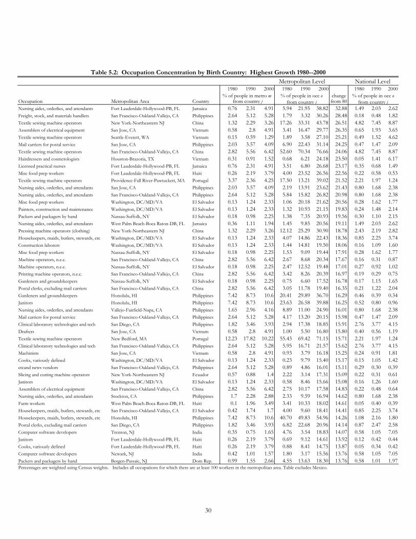
1980 1990 2000 1980 1990 2000 1980 1990 2000

changeOccupation Metropolitan Area Country from 80

Nursing aides, orderlies, and attendants Fort Lauderdale-Hollywood-PB, FL Jamaica 0.76 2.31 4.91 5.94 21.95 38.82 32.88 1.49 2.03 2.62

Freight, stock, and materials handlers San Francisco-Oakland-Vallejo, CA Philippines 2.64 5.12 5.28 1.79 3.32 30.26 28.48 0.18 0.48 1.82

Textile sewing machine operators New York-Northeastern NJ China 1.32 2.29 3.26 17.26 33.31 43.78 26.51 4.82 7.45 8.87

Assemblers of electrical equipment San Jose, CA Vietnam 0.58 2.8 4.91 3.41 16.47 29.77 26.35 0.65 1.93 3.65

Textile sewing machine operators Seattle-Everett, WA Vietnam 0.15 0.59 1.29 1.89 3.58 27.10 25.21 0.49 1.52 4.62

Mail carriers for postal service San Jose, CA Philippines 2.03 3.57 4.09 6.90 22.43 31.14 24.25 0.47 1.47 2.09

Textile sewing machine operators San Francisco-Oakland-Vallejo, CA China 2.82 5.56 6.42 52.60 70.34 76.66 24.06 4.82 7.45 8.87

Hairdressers and cosmetologists Houston-Brazoria, TX Vietnam 0.31 0.91 1.52 0.68 6.21 24.18 23.50 0.05 1.41 6.17

Licensed practical nurses Fort Lauderdale-Hollywood-PB, FL Jamaica 0.76 2.31 4.91 3.51 6.80 26.68 23.17 0.35 0.68 1.49

Misc food prep workers Fort Lauderdale-Hollywood-PB, FL Haiti 0.26 2.19 3.79 4.00 23.52 26.56 22.56 0.22 0.58 0.53

Textile sewing machine operators Providence-Fall River-Pawtuckett, MA Portugal 3.37 2.36 4.25 17.50 13.21 39.02 21.52 2.21 1.97 1.24

Nursing aides, orderlies, and attendants San Jose, CA Philippines 2.03 3.57 4.09 2.19 13.91 23.62 21.43 0.80 1.68 2.38

Nursing aides, orderlies, and attendants San Francisco-Oakland-Vallejo, CA Philippines 2.64 5.12 5.28 5.84 15.82 26.82 20.98 0.80 1.68 2.38

Misc food prep workers Washington, DC/MD/VA El Salvador 0.13 1.24 2.33 1.06 20.18 21.62 20.56 0.28 1.62 1.77

Painters, construction and maintenance Washington, DC/MD/VA El Salvador 0.13 1.24 2.33 1.32 10.93 21.15 19.83 0.24 1.48 2.14

Packers and packagers by hand Nassau-Suffolk, NY El Salvador 0.18 0.98 2.25 1.38 7.35 20.93 19.56 0.30 1.10 2.15

Nursing aides, orderlies, and attendants West Palm Beach-Boca Raton-DB, FL Jamaica 0.36 1.11 1.94 1.45 9.85 20.56 19.11 1.49 2.03 2.62

Pressing machine operators (clothing) New York-Northeastern NJ China 1.32 2.29 3.26 12.12 25.29 30.90 18.78 2.43 2.19 2.82

Housekeepers, maids, butlers, stewards, etc Washington, DC/MD/VA El Salvador 0.13 1.24 2.33 4.07 14.86 22.43 18.36 0.85 2.25 3.74

Construction laborers Washington, DC/MD/VA El Salvador 0.13 1.24 2.33 1.44 14.81 19.50 18.06 0.16 1.09 1.60

Misc food prep workers Nassau-Suffolk, NY El Salvador 0.18 0.98 2.25 1.53 9.09 19.44 17.91 0.28 1.62 1.77

Machine operators, n.e.c. San Francisco-Oakland-Vallejo, CA China 2.82 5.56 6.42 2.67 8.68 20.34 17.67 0.16 0.31 0.87

Machine operators, n.e.c. Nassau-Suffolk, NY El Salvador 0.18 0.98 2.25 2.47 12.52 19.48 17.01 0.27 0.92 1.02

Printing machine operators, n.e.c. San Francisco-Oakland-Vallejo, CA China 2.82 5.56 6.42 3.42 8.26 20.39 16.97 0.19 0.29 0.75

Gardeners and groundskeepers Nassau-Suffolk, NY El Salvador 0.18 0.98 2.25 0.75 6.60 17.52 16.78 0.17 1.15 1.65

Postal clerks, excluding mail carriers San Francisco-Oakland-Vallejo, CA China 2.82 5.56 6.42 3.05 11.78 19.40 16.35 0.21 1.22 2.04

Gardeners and groundskeepers Honolulu, HI Philippines 7.42 8.73 10.6 20.41 29.89 36.70 16.29 0.46 0.39 0.34

Janitors Honolulu, HI Philippines 7.42 8.73 10.6 23.63 26.58 39.88 16.25 0.52 0.80 0.96

Nursing aides, orderlies, and attendants Vallejo-Fairfield-Napa, CA Philippines 1.65 2.96 4.16 8.89 11.00 24.90 16.01 0.80 1.68 2.38

Mail carriers for postal service San Francisco-Oakland-Vallejo, CA Philippines 2.64 5.12 5.28 4.17 13.20 20.15 15.98 0.47 1.47 2.09

Clinical laboratory technologies and tech San Diego, CA Philippines 1.82 3.46 3.93 2.94 17.38 18.85 15.91 2.76 3.77 4.15

Drafters San Jose, CA Vietnam 0.58 2.8 4.91 1.00 5.50 16.80 15.80 0.40 0.56 1.19

Textile sewing machine operators New Bedford, MA Portugal 12.23 17.82 10.22 55.43 69.42 71.15 15.71 2.21 1.97 1.24

Clinical laboratory technologies and tech San Francisco-Oakland-Vallejo, CA Philippines 2.64 5.12 5.28 5.95 16.71 21.57 15.62 2.76 3.77 4.15

Machinists San Jose, CA Vietnam 0.58 2.8 4.91 0.93 3.79 16.18 15.25 0.24 0.91 1.81

Cooks, variously defined Washington, DC/MD/VA El Salvador 0.13 1.24 2.33 0.23 9.79 15.40 15.17 0.15 1.05 1.42

etcand news vendors San Francisco-Oakland-Vallejo, CA Philippines 2.64 5.12 5.28 0.89 4.86 16.01 15.11 0.29 0.30 0.39

Slicing and cutting machine operators New York-Northeastern NJ Ecuador 0.57 0.88 1.4 2.22 3.14 17.31 15.09 0.22 0.31 0.61

Janitors Washington, DC/MD/VA El Salvador 0.13 1.24 2.33 0.58 8.46 15.66 15.08 0.16 1.26 1.60

Assemblers of electrical equipment San Francisco-Oakland-Vallejo, CA China 2.82 5.56 6.42 2.75 10.17 17.58 14.83 0.22 0.48 0.64

Nursing aides, orderlies, and attendants Stockton, CA Philippines 1.7 2.28 2.88 2.33 9.59 16.94 14.62 0.80 1.68 2.38

Farm workers West Palm Beach-Boca Raton-DB, FL Haiti 0.1 1.96 3.49 3.41 10.33 18.02 14.61 0.05 0.40 0.39

Housekeepers, maids, butlers, stewards, etc San Francisco-Oakland-Vallejo, CA El Salvador 0.42 1.74 1.7 4.00 9.60 18.41 14.41 0.85 2.25 3.74

Housekeepers, maids, butlers, stewards, etc Honolulu, HI Philippines 7.42 8.73 10.6 40.70 49.83 54.96 14.26 1.08 2.16 1.80

Postal clerks, excluding mail carriers San Diego, CA Philippines 1.82 3.46 3.93 6.82 22.68 20.96 14.14 0.87 2.47 2.58

Computer software developers Trenton, NJ India 0.35 0.75 1.65 4.76 3.54 18.83 14.07 0.58 1.05 7.05

Janitors Fort Lauderdale-Hollywood-PB, FL Haiti 0.26 2.19 3.79 0.69 9.12 14.61 13.92 0.12 0.42 0.44

Cooks, variously defined Fort Lauderdale-Hollywood-PB, FL Haiti 0.26 2.19 3.79 0.88 8.41 14.75 13.87 0.05 0.34 0.42

Computer software developers Newark, NJ India 0.42 1.01 1.57 1.80 3.17 15.56 13.76 0.58 1.05 7.05

Packers and packagers by hand Bergen-Passaic, NJ Dom Rep. 0.99 1.55 2.66 4.55 13.63 18.30 13.76 0.58 1.01 1.97Percentages are weighted using Census weights. Includes all occupations for which there are at least 100 workers in the metropolitan area. Table excludes Mexico.

from country jfrom country j

Table 5.2: Occupation Concentration by Birth Country: Highest Growth 1980--2000

Metropolitan Level

% of people in occ o

National Level

% of people in occ o % of people in metro m from country j

30

Country of Origin 1980 1990 2000 1980 1990 2000 Country of Origin 1980 1990 2000 1980 1990 2000

American Samoa 1 1.00 Jordan 1 1.00

Guam 2 1 1.00 1.00 Lebanon 3 2 0.60 0.40

Puerto Rico 3 11 18 0.27 0.35 0.41 Syria 1 1 1.00 0.50

U.S. Virgin Islands 1 1 1 1.00 1.00 1.00 Turkey 2 2 1.00 0.50

Other US Possessions 1 1.00 AFRICA 4 0.80

Canada 5 5 11 0.22 0.14 0.31 Australia and NZ 1 4 1.00 1.00

Atlantic Islands 1 2 1.00 1.00 Abroad (unknown) 6 14 0.75 0.47

Mexico 7 15 19 0.27 0.22 0.16 Belize 1 1 0.50 0.50

Cuba 5 9 8 0.50 0.45 0.47 Costa Rica 2 3 1.00 0.75

West Indies 1 1 1 1.00 1.00 1.00 El Salvador 3 8 8 1.00 0.47 0.36

England 2 4 7 0.22 0.15 0.25 Guatemala 1 3 7 1.00 0.27 0.33

Scotland 2 1 1 1.00 0.50 1.00 Honduras 1 4 8 1.00 1.00 0.62

United Kingdom, ns 1 5 0.25 0.71 Nicaragua 2 6 6 1.00 0.86 0.75

Ireland 4 6 5 1.00 0.75 0.71 Panama 1 3 3 1.00 0.75 1.00

France 2 3 2 0.67 0.75 0.29 Dominican Republic 1 7 8 1.00 0.78 0.53

Netherlands 1 1 1 1.00 1.00 1.00 Haiti 2 4 3 0.67 0.50 0.23

Switerland 1 1 1.00 1.00 Jamaica 1 2 4 0.50 0.14 0.21

Albania 2 1.00 Antigua-Barbuda 1 1 1.00 1.00

Greece 2 2 4 0.67 0.25 0.40 Bahamas 1 1 1.00 1.00

Italy 6 9 8 0.35 0.43 0.42 Barbados 1 1 1 1.00 1.00 1.00

Portugal 3 5 6 0.50 0.38 0.60 Dominica 1 1 1.00 1.00

Spain 1 4 3 1.00 1.00 1.00 Grenada 1 1 1.00 1.00

Austria 1 1 1 1.00 1.00 1.00 St. Kitts-Nevis 1 1.00

Bulgaria 1 1.00 St. Lucia 1 1.00

Czechoslovakia 1 3 2 1.00 1.00 1.00 St. Vincent 1 1 1.00 1.00

Germany 4 6 15 0.22 0.10 0.24 Trinidad and Tobago 1 2 3 1.00 0.50 0.43

Hungary 1 1 1 0.50 0.50 0.50 Argentina 2 4 4 1.00 0.80 0.80

Poland 4 4 9 0.67 0.33 0.69 Bolivia 1 2 1.00 1.00

Romania 1 3 5 1.00 1.00 1.00 Brazil 3 5 0.60 0.45

Yugoslavia 3 4 7 0.75 0.67 0.78 Chile 1 2 0.25 0.67

Lithuania 1 1 1.00 1.00 Colombia 3 7 9 1.00 0.50 0.47

Other USSR/Russia 2 5 7 0.50 0.71 0.30 Ecuador 3 6 7 1.00 0.67 0.70

Europe, ns 1 1.00 Guyana/British Guiana 1 2 4 1.00 0.67 0.67

China 4 8 9 0.33 0.31 0.23 Peru 3 7 10 1.00 0.70 0.71

Japan 3 5 7 0.60 0.31 0.35 Uruguay 1 1.00

Korea 3 6 10 0.60 0.30 0.37 Venezuela 1 2 1.00 1.00

Cambodia (Kampuchea) 3 3 1.00 0.50 South Korea 2 1 0.40 0.20

Indonesia 1 1 2 1.00 1.00 1.00 Bangladesh 1 2 1.00 1.00

Laos 1 2 1.00 0.29 Myanmar 2 3 1.00 1.00

Malaysia 2 1.00 Pakistan 3 5 0.75 0.56

Philippines 8 9 7 0.67 0.24 0.16 Egypt 3 3 2 0.75 1.00 0.67

Thailand 1 3 2 1.00 1.00 0.40 Morocco 2 1.00

Vietnam 8 10 7 0.89 0.45 0.21 Ghana 2 1 1.00 0.50

Southeast Asia, ns 1 0.50 Liberia 1 1.00

Afghanistan 1 2 1.00 1.00 Nigeria 3 3 1.00 0.33

India 3 6 7 0.50 0.29 0.16 Sierra Leone 1 1.00

Iran 1 5 5 1.00 0.50 0.33 Ethiopia 1 2 1.00 0.67

Iraq 1 3 2 1.00 1.00 0.50 South Africa 1 2 1.00 1.00

Israel/Palestine 2 3 3 1.00 0.60 0.75 Fiji 3 0.72 1.00

average (weighted by the country share of total immigrants) 0.29 0.35 0.45

* This counts the number of occupations that are ranked 1 across metropolitan areas. In some metro area, some occupations are tied for 1. Based on weighted data

No. of Unique Top

Occupations Across

Metro-Areas

No. of Popular

Occupations / No.

of Metro-Areas *

Table 5.3: Distribution of Distinct Popular Occupations Across Metro Areas by Country of Origin

No. of Popular

Occupations / No.

of Metro-Areas *

No. of Unique Top

Occupations Across

Metro-Areas

31

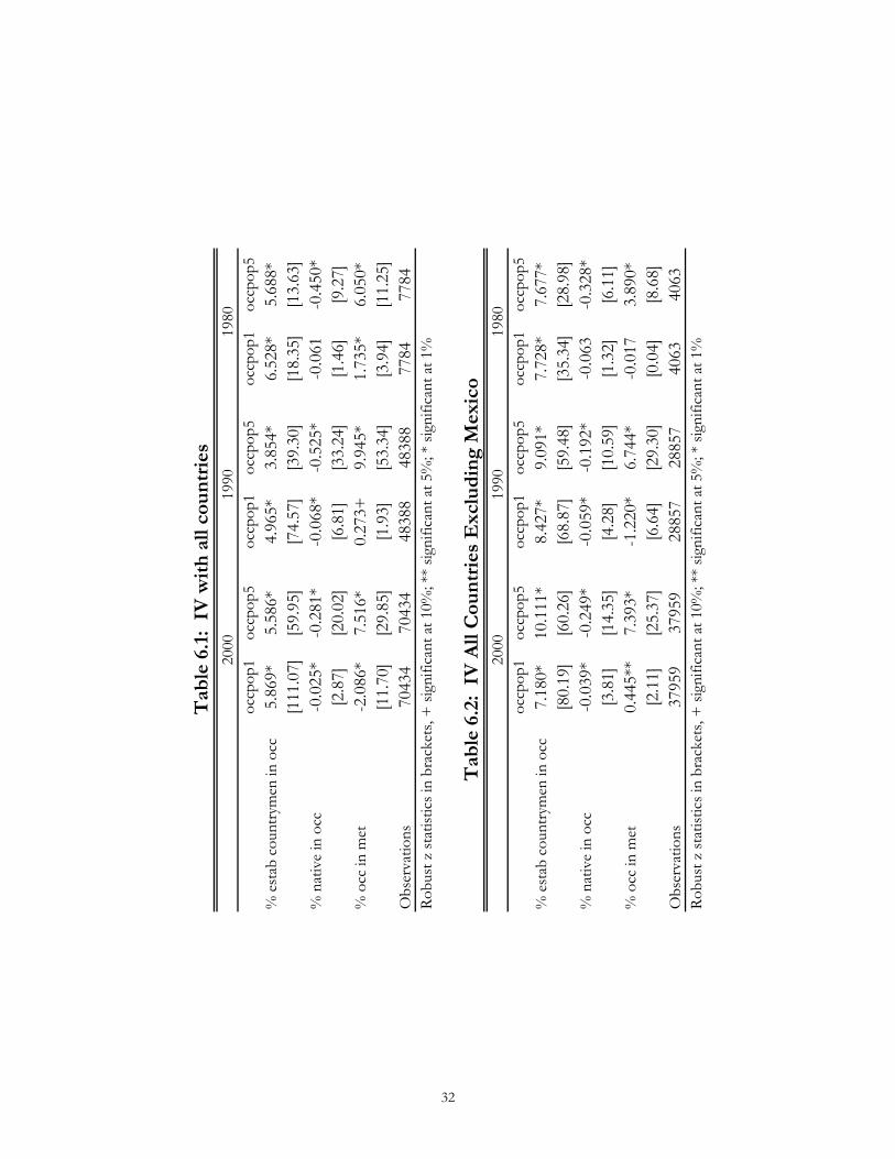
occ

pop1

occ

pop5

occ

pop1

occ

pop5

occ

pop1

occ

pop5

% e

stab

countrym

en in o

cc5.8

69*

5.5

86*

4.9

65*

3.8

54*

6.5

28*

5.6

88*

[111.0

7]

[59.9

5]

[74.5

7]

[39.3

0]

[18.3

5]

[13.6

3]

% n

ativ

e in

occ

-0.0

25*

-0.2

81*

-0.0

68*

-0.5

25*

-0.0

61

-0.4

50*

[2.8

7]

[20.0

2]

[6.8

1]

[33.2

4]

[1.4

6]

[9.2

7]

% o

cc in m

et-2

.086*

7.5

16*

0.2

73+

9.9

45*

1.7

35*

6.0

50*

[11.7

0]

[29.8

5]

[1.9

3]

[53.3

4]

[3.9

4]

[11.2

5]

Obse

rvat

ions

70434

70434

48388

48388

7784

7784

occ

pop1

occ

pop5

occ

pop1

occ

pop5

occ

pop1

occ

pop5

% e

stab

countrym

en in o

cc7.1

80*

10.1

11*

8.4

27*

9.0

91*

7.7

28*

7.6

77*

[80.1

9]

[60.2

6]

[68.8

7]

[59.4

8]

[35.3

4]

[28.9

8]

% n

ativ

e in

occ

-0.0

39*

-0.2

49*

-0.0

59*

-0.1

92*

-0.0

63

-0.3

28*

[3.8

1]

[14.3

5]

[4.2

8]

[10.5

9]

[1.3

2]

[6.1

1]

% o

cc in m

et0.4

45**

7.3

93*

-1.2

20*

6.7

44*

-0.0

17

3.8

90*

[2.1

1]

[25.3

7]

[6.6

4]

[29.3

0]

[0.0

4]

[8.6

8]

Obse

rvat

ions

37959

37959

28857

28857

4063

4063

Robust

z sta

tist

ics in

bra

cket

s, +

sig

nific

ant at

10%

; **

sig

nific

ant at

5%

; *

sign

ific

ant at

1%

Robust

z sta

tist

ics in

bra

cket

s, +

sig

nific

ant at

10%

; **

sig

nific

ant at

5%

; *

sign

ific

ant at

1%

Table 6.2: IV All Countries Excluding Mexico

2000

1990

1980

Table 6.1: IV with all countries

2000

1990

1980

32

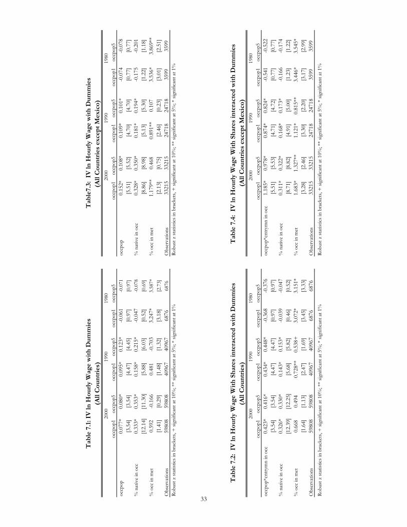
occpop1

occpop5

occpop1

occpop5

occpop1

occpop5

occpop1

occpop5

occpop1

occpop5

occpop1

occpop5

occpop

0.077*

0.080*

0.095*

0.123*

-0.061

-0.071

occpop

0.152*

0.108*

0.109*

0.101*

-0.074

-0.078

[3.54]

[3.54]

[4.47]

[4.45]

[0.97]

[0.97]

[5.51]

[5.52]

[4.70]

[4.70]

[0.77]

[0.77]

% native in occ

0.333*

0.353*

0.158*

0.215*

-0.047

-0.078

% native in occ

0.328*

0.350*

0.181*

0.194*

-0.175

-0.201

[12.14]

[11.30]

[5.88]

[6.03]

[0.52]

[0.69]

[8.86]

[8.98]

[5.13]

[5.30]

[1.22]

[1.18]

% occ in m

et0.592

-0.166

0.481

-0.703

3.247*

3.587*

% occ in m

et1.179**

0.468

0.891**

0.107

3.536*

3.869**

[1.41]

[0.29]

[1.48]

[1.32]

[3.18]

[2.73]

[2.13]

[0.75]

[2.46]

[0.23]

[3.01]

[2.51]

Observations

59808

59808

40967

40967

6876

6876

Observations

33215

33215

24718

24718

3599

3599

occpop1

occpop5

occpop1

occpop5

occpop1

occpop5

occpop1

occpop5

occpop1

occpop5

occpop1

occpop5

occpop*c

ntrym

n in occ

0.423*

0.416*

0.434*

0.448*

-0.368

-0.376

occpop*c

ntrym

n in occ

1.185*

0.978*

0.874*

0.824*

-0.541

-0.522

[3.54]

[3.54]

[4.47]

[4.47]

[0.97]

[0.97]

[5.51]

[5.53]

[4.71]

[4.72]

[0.77]

[0.77]

% native in occ

0.326*

0.330*

0.143*

0.153*

-0.039

-0.047

% native in occ

0.311*

0.322*

0.168*

0.173*

-0.166

-0.174

[12.39]

[12.25]

[5.68]

[5.82]

[0.46]

[0.52]

[8.71]

[8.82]

[4.91]

[5.00]

[1.23]

[1.22]

% occ in m

et0.668

0.494

0.728**

0.538+

3.072*

3.151*

% occ in m

et1.683*

1.327**

1.121*

0.815**

3.446*

3.545*

[1.64]

[1.13]

[2.47]

[1.69]

[3.45]

[3.33]

[3.28]

[2.46]

[3.30]

[2.20]

[3.17]

[2.99]

Observations

59808

59808

40967

40967

6876

6876

Observations

33215

33215

24718

24718

3599

3599

Robust z statistics in brack

ets, +

significan

t at 10%; **

significan

t at 5%; * sign

ifican

t at 1%

Robust z statistics in brack

ets, +

significan

t at 10%; **

significan

t at 5%; * sign

ifican

t at 1%

(All Countries)

Table7.3: IV ln H

ourly W

age w

ith D

ummies

Table 7.4: IV ln H

ourly W

age W

ith Shares interacted w

ith D

ummies

(All Countries except Mexico)

2000

1990

1980

2000

1990

1980

(All Countries except Mexico)

(All Countries)

Table 7.1: IV

ln H

ourly W

age w

ith D

ummies

2000

1990

1980

Robust z statistics in brack

ets, +

significan

t at 10%; **

significan

t at 5%; * sign

ifican

t at 1%

Robust z statistics in brack

ets, +

significan

t at 10%; **

significan

t at 5%; * sign

ifican

t at 1%

Table 7.2: IV ln H

ourly W

age W

ith Shares interacted w

ith D

ummies

2000

1990

1980

33

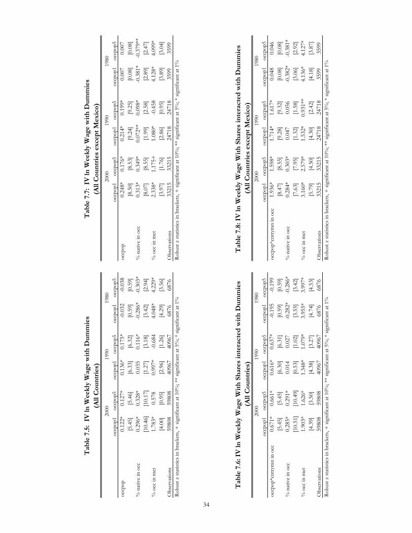
occ

pop1

occ

pop5

occ

pop1

occ

pop5

occ

pop1

occ

pop5

occ

pop1

occ

pop5

occ

pop1

occ

pop5

occ

pop1

occ

pop5

occ

pop

0.1

22*

0.1

27*

0.1

36*

0.1

75*

-0.0

32

-0.0

38

occ

pop

0.2

48*

0.1

76*

0.2

14*

0.1

99*

0.0

07

0.0

07

[5.4

5]

[5.4

6]

[6.3

3]

[6.3

2]

[0.5

9]

[0.5

9]

[8.5

0]

[8.5

3]

[9.2

4]

[9.2

5]

[0.0

8]

[0.0

8]

% n

ativ

e in

occ

0.2

96*

0.3

28*

0.0

35

0.1

16*

-0.2

86*

-0.3

03*

% n

ativ

e in

occ

0.3

13*

0.3

49*

0.0

72**

0.0

98*

-0.3

81*

-0.3

79**

[10.4

6]

[10.1

7]

[1.2

7]

[3.1

8]

[3.4

2]

[2.9

4]

[8.0

7]

[8.5

5]

[1.9

9]

[2.5

8]

[2.8

9]

[2.4

7]

% o

cc in m

et1.7

83*

0.5

78

0.9

97*

-0.6

84

4.0

48*

4.2

29*

% o

cc in m

et2.3

38*

1.1

75+

1.0

80*

-0.4

58

4.1

28*

4.0

99*

[4.0

0]

[0.9

5]

[2.9

6]

[1.2

6]

[4.2

9]

[3.5

6]

[3.9

7]

[1.7

6]

[2.8

6]

[0.9

5]

[3.8

9]

[3.0

4]

Obse

rvat

ions

59808

59808

40967

40967

6876

6876

Obse

rvat

ions

33215

33215

24718

24718

3599

3599

occ

pop1

occ

pop5

occ

pop1

occ

pop5

occ

pop1

occ

pop5

occ

pop1

occ

pop5

occ

pop1

occ

pop5

occ

pop1

occ

pop5

occ

pop*c

ntrym

n in o

cc0.6

71*

0.6

61*

0.6

16*

0.6

37*

-0.1

95

-0.1

99

occ

pop*c

ntrym

n in o

cc1.9

36*

1.5

98*

1.7

14*

1.6

17*

0.0

48

0.0

46

[5.4

5]

[5.4

5]

[6.3

0]

[6.3

1]

[0.5

9]

[0.5

9]

[8.4

7]

[8.5

5]

[9.2

8]

[9.3

2]

[0.0

8]

[0.0

8]

% n

ativ

e in

occ

0.2

85*

0.2

91*

0.0

14

0.0

27

-0.2

82*

-0.2

86*

% n

ativ

e in

occ

0.2

84*

0.3

03*

0.0

47

0.0

56

-0.3

82*

-0.3

81*

[10.5

1]

[10.4

9]

[0.5

3]

[1.0

2]

[3.5

5]

[3.4

2]

[7.6

3]

[7.9

5]

[1.3

2]

[1.5

8]

[3.0

6]

[2.9

2]

% o

cc in m

et1.9

03*

1.6

26*

1.3

48*

1.0

79*

3.9

55*

3.9

97*

% o

cc in m

et3.1

60*

2.5

79*

1.5

32*

0.9

31**

4.1

36*

4.1

27*

[4.3

9]

[3.5

0]

[4.3

8]

[3.2

7]

[4.7

4]

[4.5

3]

[5.7

9]

[4.5

0]

[4.3

0]

[2.4

2]

[4.1

8]

[3.8

7]

Obse

rvat

ions

59808

59808

40967

40967

6876

6876

Obse

rvat

ions

33215

33215

24718

24718

3599

3599

Robust z

sta

tistics in

bra

cket

s, +

sig

nifican

t at

10%

; **

sig

nifican

t at

5%

; *

sign

ifican

t at

1%

Robust z

sta

tistics in

bra

cket

s, +

sig

nifican

t at

10%

; **

sig

nifican

t at

5%

; *

sign

ifican

t at

1%

Table 7.8: IV ln Weekly Wage With Shares interacted with Dummies

(All Countries except Mexico)

2000

1990

1980

Table 7.7: IV ln Weekly Wage with Dummies

(All Countries except Mexico)

2000

1990

1980

Table 7.5: IV ln Weekly Wage with Dummies

2000

1990

1980

(All Countries)

Robust z

sta

tistics in

bra

cket

s, +

sig

nifican

t at

10%

; **

sig

nifican

t at

5%

; *

sign

ifican

t at

1%

Robust z

sta

tistics in

bra

cket

s, +

sig

nifican

t at

10%

; **

sig

nifican

t at

5%

; *

sign

ifican

t at

1%

Table 7.6: IV ln Weekly Wage With Shares interacted with Dummies

2000

1990

1980

(All Countries)

34

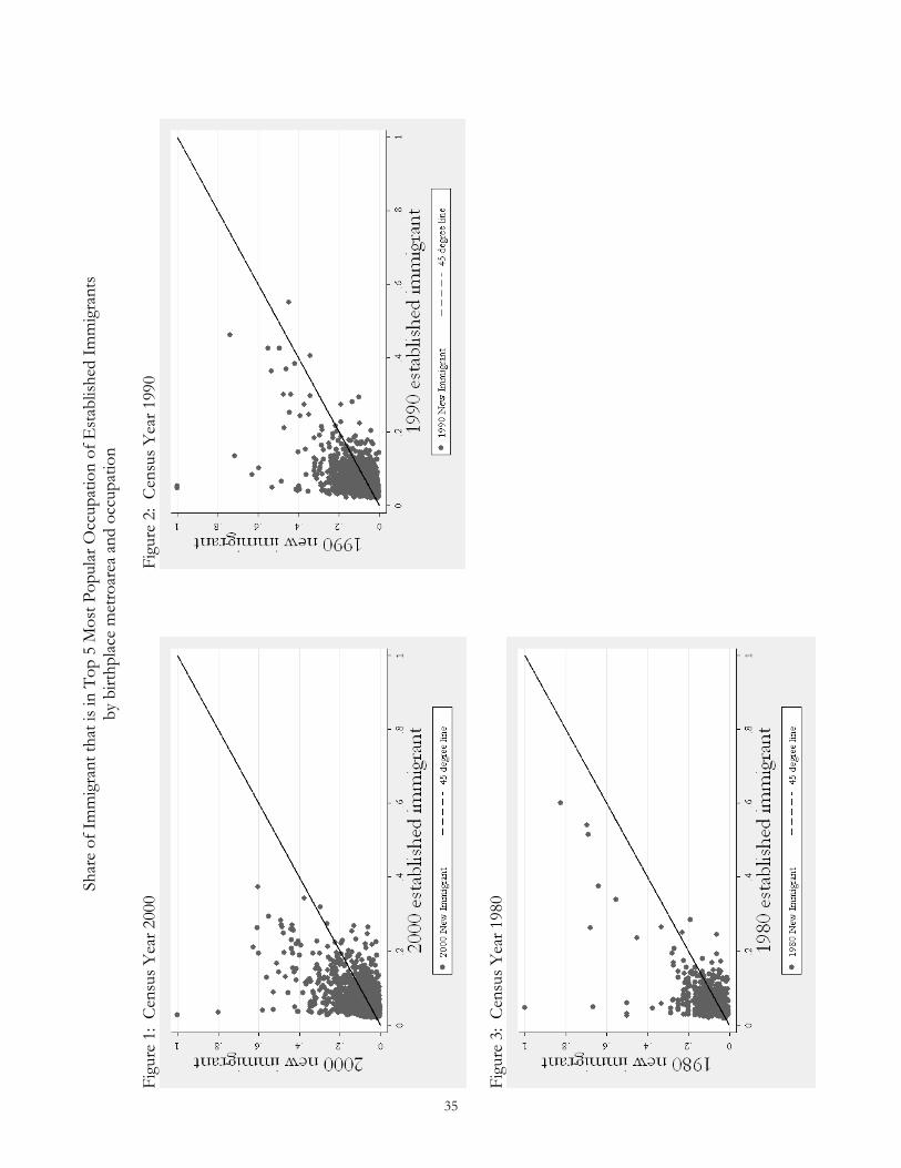
Share of Immigrant that is in Top 5 Most Popular Occupation of Established Immigrants

by birthplace metroarea and occupation

Figure 1: Census Year 2000

Figure 2: Census Year 1990

Figure 3: Census Year 1980

35

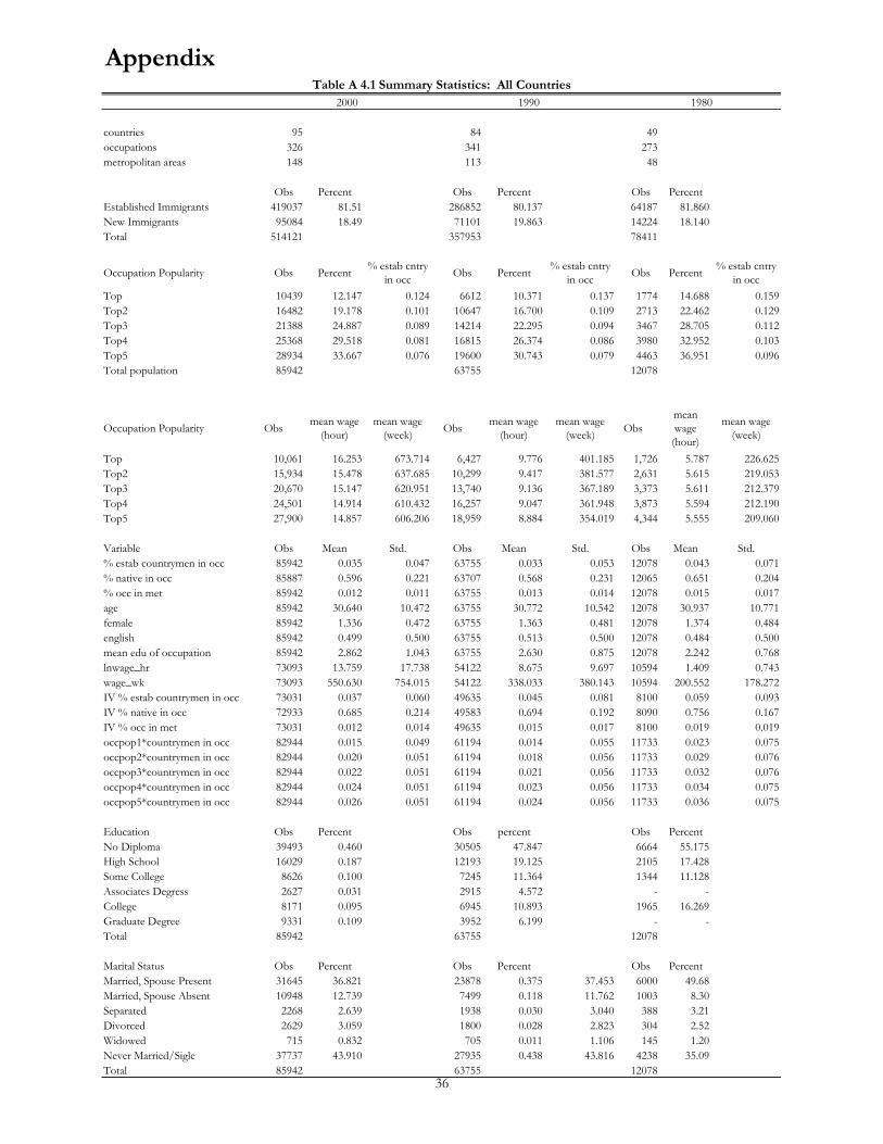
Appendix

countries 95 84 49

occupations 326 341 273

metropolitan areas 148 113 48

Obs Percent Obs Percent Obs Percent

Established Immigrants 419037 81.51 286852 80.137 64187 81.860

New Immigrants 95084 18.49 71101 19.863 14224 18.140

Total 514121 357953 78411

Occupation Popularity Obs Percent% estab cntry

in occObs Percent

% estab cntry

in occObs Percent

% estab cntry

in occ

Top 10439 12.147 0.124 6612 10.371 0.137 1774 14.688 0.159

Top2 16482 19.178 0.101 10647 16.700 0.109 2713 22.462 0.129

Top3 21388 24.887 0.089 14214 22.295 0.094 3467 28.705 0.112

Top4 25368 29.518 0.081 16815 26.374 0.086 3980 32.952 0.103

Top5 28934 33.667 0.076 19600 30.743 0.079 4463 36.951 0.096

Total population 85942 63755 12078

Occupation Popularity Obsmean wage

(hour)

mean wage

(week)Obs

mean wage

(hour)

mean wage

(week)Obs

mean

wage

(hour)

mean wage

(week)

Top 10,061 16.253 673.714 6,427 9.776 401.185 1,726 5.787 226.625

Top2 15,934 15.478 637.685 10,299 9.417 381.577 2,631 5.615 219.053

Top3 20,670 15.147 620.951 13,740 9.136 367.189 3,373 5.611 212.379

Top4 24,501 14.914 610.432 16,257 9.047 361.948 3,873 5.594 212.190

Top5 27,900 14.857 606.206 18,959 8.884 354.019 4,344 5.555 209.060

Variable Obs Mean Std. Obs Mean Std. Obs Mean Std.

% estab countrymen in occ 85942 0.035 0.047 63755 0.033 0.053 12078 0.043 0.071

% native in occ 85887 0.596 0.221 63707 0.568 0.231 12065 0.651 0.204

% occ in met 85942 0.012 0.011 63755 0.013 0.014 12078 0.015 0.017

age 85942 30.640 10.472 63755 30.772 10.542 12078 30.937 10.771

female 85942 1.336 0.472 63755 1.363 0.481 12078 1.374 0.484

english 85942 0.499 0.500 63755 0.513 0.500 12078 0.484 0.500

mean edu of occupation 85942 2.862 1.043 63755 2.630 0.875 12078 2.242 0.768

lnwage_hr 73093 13.759 17.738 54122 8.675 9.697 10594 1.409 0.743

wage_wk 73093 550.630 754.015 54122 338.033 380.143 10594 200.552 178.272

IV % estab countrymen in occ 73031 0.037 0.060 49635 0.045 0.081 8100 0.059 0.093

IV % native in occ 72933 0.685 0.214 49583 0.694 0.192 8090 0.756 0.167

IV % occ in met 73031 0.012 0.014 49635 0.015 0.017 8100 0.019 0.019

occpop1*countrymen in occ 82944 0.015 0.049 61194 0.014 0.055 11733 0.023 0.075

occpop2*countrymen in occ 82944 0.020 0.051 61194 0.018 0.056 11733 0.029 0.076

occpop3*countrymen in occ 82944 0.022 0.051 61194 0.021 0.056 11733 0.032 0.076

occpop4*countrymen in occ 82944 0.024 0.051 61194 0.023 0.056 11733 0.034 0.075

occpop5*countrymen in occ 82944 0.026 0.051 61194 0.024 0.056 11733 0.036 0.075

Education Obs Percent Obs percent Obs Percent

No Diploma 39493 0.460 30505 47.847 6664 55.175

High School 16029 0.187 12193 19.125 2105 17.428

Some College 8626 0.100 7245 11.364 1344 11.128

Associates Degress 2627 0.031 2915 4.572 - -

College 8171 0.095 6945 10.893 1965 16.269

Graduate Degree 9331 0.109 3952 6.199 - -

Total 85942 63755 12078

Marital Status Obs Percent Obs Percent Obs Percent

Married, Spouse Present 31645 36.821 23878 0.375 37.453 6000 49.68

Married, Spouse Absent 10948 12.739 7499 0.118 11.762 1003 8.30

Separated 2268 2.639 1938 0.030 3.040 388 3.21

Divorced 2629 3.059 1800 0.028 2.823 304 2.52

Widowed 715 0.832 705 0.011 1.106 145 1.20

Never Married/Sigle 37737 43.910 27935 0.438 43.816 4238 35.09

Total 85942 63755 12078

Table A 4.1 Summary Statistics: All Countries

2000 1990 1980

36

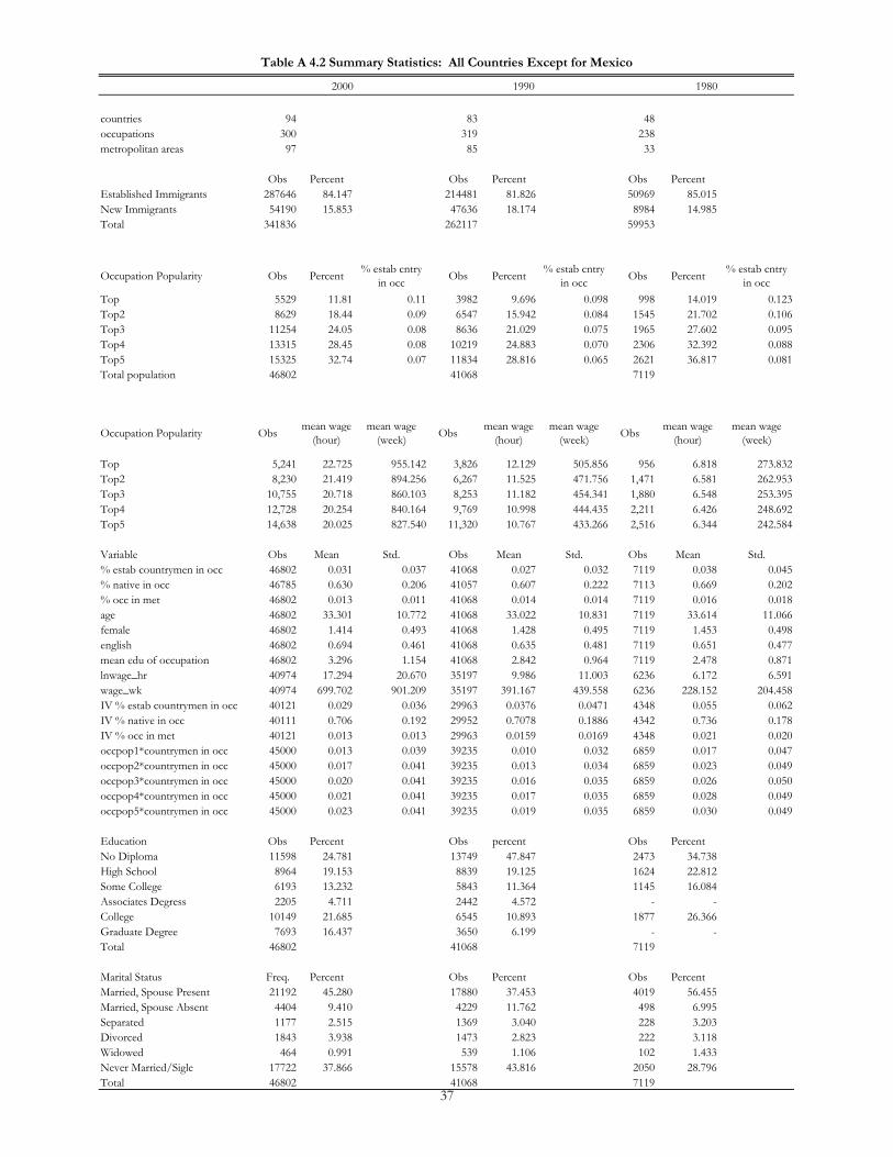
countries 94 83 48

occupations 300 319 238

metropolitan areas 97 85 33

Obs Percent Obs Percent Obs Percent

Established Immigrants 287646 84.147 214481 81.826 50969 85.015

New Immigrants 54190 15.853 47636 18.174 8984 14.985

Total 341836 262117 59953

Occupation Popularity Obs Percent% estab cntry

in occObs Percent

% estab cntry

in occObs Percent

% estab cntry

in occ

Top 5529 11.81 0.11 3982 9.696 0.098 998 14.019 0.123

Top2 8629 18.44 0.09 6547 15.942 0.084 1545 21.702 0.106

Top3 11254 24.05 0.08 8636 21.029 0.075 1965 27.602 0.095

Top4 13315 28.45 0.08 10219 24.883 0.070 2306 32.392 0.088

Top5 15325 32.74 0.07 11834 28.816 0.065 2621 36.817 0.081

Total population 46802 41068 7119

Occupation Popularity Obsmean wage

(hour)

mean wage

(week)Obs

mean wage

(hour)

mean wage

(week)Obs

mean wage

(hour)

mean wage

(week)

Top 5,241 22.725 955.142 3,826 12.129 505.856 956 6.818 273.832

Top2 8,230 21.419 894.256 6,267 11.525 471.756 1,471 6.581 262.953

Top3 10,755 20.718 860.103 8,253 11.182 454.341 1,880 6.548 253.395

Top4 12,728 20.254 840.164 9,769 10.998 444.435 2,211 6.426 248.692

Top5 14,638 20.025 827.540 11,320 10.767 433.266 2,516 6.344 242.584

Variable Obs Mean Std. Obs Mean Std. Obs Mean Std.

% estab countrymen in occ 46802 0.031 0.037 41068 0.027 0.032 7119 0.038 0.045

% native in occ 46785 0.630 0.206 41057 0.607 0.222 7113 0.669 0.202

% occ in met 46802 0.013 0.011 41068 0.014 0.014 7119 0.016 0.018

age 46802 33.301 10.772 41068 33.022 10.831 7119 33.614 11.066

female 46802 1.414 0.493 41068 1.428 0.495 7119 1.453 0.498

english 46802 0.694 0.461 41068 0.635 0.481 7119 0.651 0.477

mean edu of occupation 46802 3.296 1.154 41068 2.842 0.964 7119 2.478 0.871

lnwage_hr 40974 17.294 20.670 35197 9.986 11.003 6236 6.172 6.591

wage_wk 40974 699.702 901.209 35197 391.167 439.558 6236 228.152 204.458

IV % estab countrymen in occ 40121 0.029 0.036 29963 0.0376 0.0471 4348 0.055 0.062

IV % native in occ 40111 0.706 0.192 29952 0.7078 0.1886 4342 0.736 0.178

IV % occ in met 40121 0.013 0.013 29963 0.0159 0.0169 4348 0.021 0.020

occpop1*countrymen in occ 45000 0.013 0.039 39235 0.010 0.032 6859 0.017 0.047

occpop2*countrymen in occ 45000 0.017 0.041 39235 0.013 0.034 6859 0.023 0.049

occpop3*countrymen in occ 45000 0.020 0.041 39235 0.016 0.035 6859 0.026 0.050

occpop4*countrymen in occ 45000 0.021 0.041 39235 0.017 0.035 6859 0.028 0.049

occpop5*countrymen in occ 45000 0.023 0.041 39235 0.019 0.035 6859 0.030 0.049

Education Obs Percent Obs percent Obs Percent

No Diploma 11598 24.781 13749 47.847 2473 34.738

High School 8964 19.153 8839 19.125 1624 22.812

Some College 6193 13.232 5843 11.364 1145 16.084

Associates Degress 2205 4.711 2442 4.572 - -

College 10149 21.685 6545 10.893 1877 26.366

Graduate Degree 7693 16.437 3650 6.199 - -

Total 46802 41068 7119

Marital Status Freq. Percent Obs Percent Obs Percent

Married, Spouse Present 21192 45.280 17880 37.453 4019 56.455

Married, Spouse Absent 4404 9.410 4229 11.762 498 6.995

Separated 1177 2.515 1369 3.040 228 3.203

Divorced 1843 3.938 1473 2.823 222 3.118

Widowed 464 0.991 539 1.106 102 1.433

Never Married/Sigle 17722 37.866 15578 43.816 2050 28.796

Total 46802 41068 7119

1990 1980

Table A 4.2 Summary Statistics: All Countries Except for Mexico

2000

37

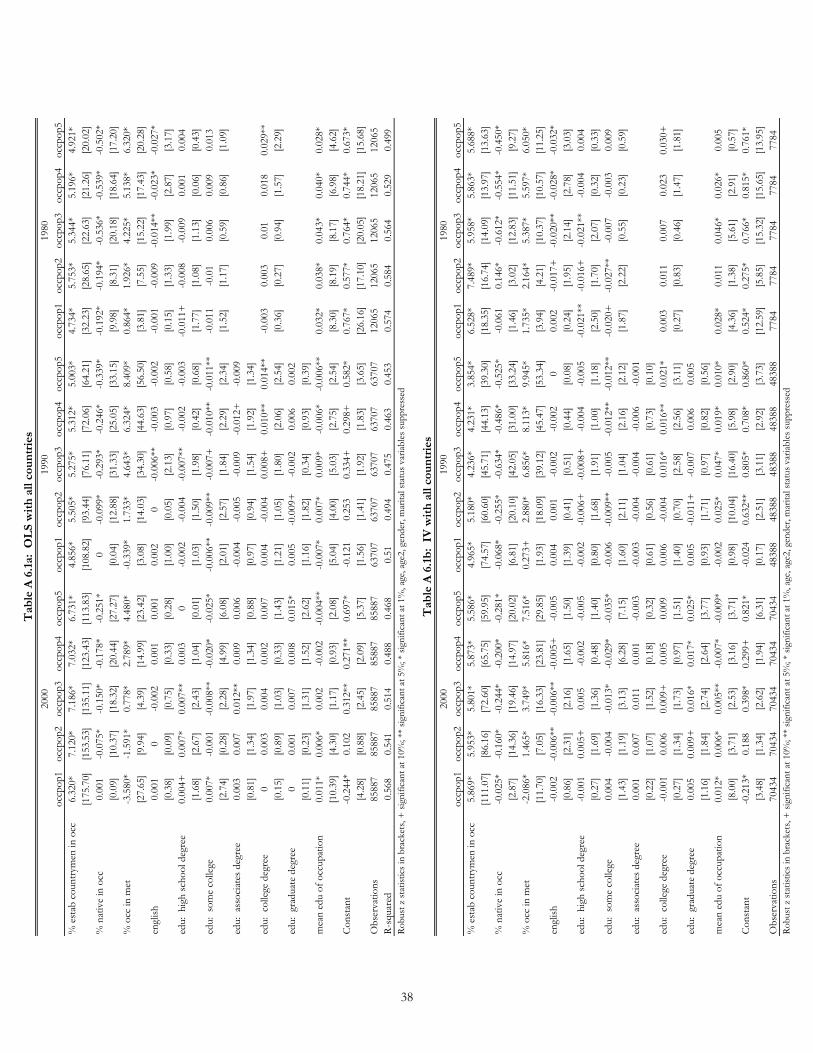
occ

pop1

occ

pop2

occ

pop3

occ

pop4

occ

pop5

occ

pop1

occ

pop2

occ

pop3

occ

pop4

occ

pop5

occ

pop1

occ

pop2

occ

pop3

occ

pop4

occ

pop5

% e

stab

countrym

en in o

cc6.3

20*

7.1

20*

7.1

86*

7.0

32*

6.7

31*

4.8

56*

5.5

05*

5.2

75*

5.3

12*

5.0

03*

4.7

34*

5.7

53*

5.3

44*

5.1

96*

4.9

21*

[175.7

0]

[153.5

3]

[135.1

1]

[123.4

3]

[113.8

3]

[108.8

2]

[93.4

4]

[76.1

1]

[72.0

6]

[64.2

1]

[32.2

3]

[28.6

5]

[22.6

3]

[21.2

6]

[20.0

2]

% n

ativ

e in

occ

0.0

01

-0.0

75*

-0.1

50*

-0.1

78*

-0.2

51*

0-0

.099*

-0.2

93*

-0.2

46*

-0.3

39*

-0.1

92*

-0.1

94*

-0.5

36*

-0.5

39*

-0.5

02*

[0.0

9]

[10.3

7]

[18.3

2]

[20.4

4]

[27.2

7]

[0.0

4]

[12.8

8]

[31.3

3]

[25.0

5]

[33.1

5]

[9.9

8]

[8.3

1]

[20.1

8]

[18.6

4]

[17.2

0]

% o

cc in m

et-3

.580*

-1.5

91*

0.7

78*

2.7

89*

4.4

80*

-0.3

39*

1.7

33*

4.6

43*

6.3

24*

8.4

09*

0.8

64*

1.9

26*

4.2

25*

5.1

38*

6.3

20*

[27.6

5]

[9.9

4]

[4.3

9]

[14.9

9]

[23.4

2]

[3.0

8]

[14.0

3]

[34.3

0]

[44.6

3]

[56.5

0]

[3.8

1]

[7.5

5]

[15.2

2]

[17.4

3]

[20.2

8]

engl

ish

0.0

01

0-0

.002

0.0

01

0.0

01

0.0

02

0-0

.006**

-0.0

03

-0.0

02

-0.0

01

-0.0

09

-0.0

14**

-0.0

23*

-0.0

27*

[0.3

8]

[0.0

9]

[0.7

5]

[0.3

3]

[0.2

8]

[1.0

0]

[0.0

5]

[2.1

3]

[0.9

7]

[0.5

8]

[0.1

5]

[1.3

3]

[1.9

9]

[2.8

7]

[3.1

7]

edu: h

igh sch

ool deg

ree

0.0

04+

0.0

07*

0.0

07**

0.0

03

0-0

.002

-0.0

04

-0.0

07**

-0.0

02

-0.0

03

-0.0

11+

-0.0

08

-0.0

09

0.0

01

0.0

04

[1.6

8]

[2.6

7]

[2.4

3]

[1.0

4]

[0.0

1]

[1.0

3]

[1.5

0]

[1.9

8]

[0.4

2]

[0.6

8]

[1.7

7]

[1.0

8]

[1.1

3]

[0.0

6]

[0.4

3]

edu: som

e co

lleg

e0.0

07*

-0.0

01

-0.0

08**

-0.0

20*

-0.0

25*

-0.0

06**

-0.0

09**

-0.0

07+

-0.0

10**

-0.0

11**

-0.0

11

-0.0

10.0

06

0.0

09

0.0

13

[2.7

4]

[0.2

8]

[2.2

8]

[4.9

9]

[6.0

8]

[2.0

1]

[2.5

7]

[1.8

4]

[2.2

9]

[2.3

4]

[1.5

2]

[1.1

7]

[0.5

9]

[0.8

6]

[1.0

9]

edu: a

ssoci

ates

deg

ree

0.0

03

0.0

07

0.0

12**

0.0

09

0.0

06

-0.0

04

-0.0

05

-0.0

09

-0.0

12+

-0.0

09

[0.8

1]

[1.3

4]

[1.9

7]

[1.3

4]

[0.8

8]

[0.9

7]

[0.9

4]

[1.5

4]

[1.9

2]

[1.3

4]

edu: c

olleg

e deg

ree

00.0

03

0.0

04

0.0

02

0.0

07

0.0

04

-0.0

04

0.0

08+

0.0

10**

0.0

14**

-0.0

03

0.0

03

0.0

10.0

18

0.0

29**

[0.1

5]

[0.8

9]

[1.0

3]

[0.3

3]

[1.4

3]

[1.2

1]

[1.0

5]

[1.8

0]

[2.0

6]

[2.5

4]

[0.3

6]

[0.2

7]

[0.9

4]

[1.5

7]

[2.2

9]

edu: g

raduat

e deg

ree

00.0

01

0.0

07

0.0

08

0.0

15*

0.0

05

-0.0

09+

-0.0

02

0.0

06

0.0

02

[0.1

1]

[0.2

3]

[1.3

1]

[1.5

2]

[2.6

2]

[1.1

6]

[1.8

2]

[0.3

4]

[0.9

3]

[0.3

9]

mea

n e

du o

f occ

upat

ion

0.0

11*

0.0

06*

0.0

02

-0.0

02

-0.0

04**

-0.0

07*

0.0

07*

0.0

09*

-0.0

06*

-0.0

06**

0.0

32*

0.0

38*

0.0

43*

0.0

40*

0.0

28*

[10.3

9]

[4.3

0]

[1.1

7]

[0.9

3]

[2.0

8]

[5.0

4]

[4.0

0]

[5.0

3]

[2.7

5]

[2.5

4]

[8.3

0]

[8.1

9]

[8.1

7]

[6.9

8]

[4.6

2]

Const

ant

-0.2

44*

0.1

02

0.3

12**

0.2

71**

0.6

97*

-0.1

21

0.2

53

0.3

34+

0.2

98+

0.5

82*

0.7

67*

0.5

77*

0.7

64*

0.7

44*

0.6

73*

[4.2

8]

[0.8

8]

[2.4

5]

[2.0

9]

[5.3

7]

[1.5

6]

[1.4

1]

[1.9

2]

[1.8

3]

[3.6

5]

[26.1

6]

[17.1

0]

[20.0

5]

[18.2

1]

[15.6

8]

Obse

rvat

ions

85887

85887

85887

85887

85887

63707

63707

63707

63707

63707

12065

12065

12065

12065

12065

R-s

quar

ed0.5

68

0.5

41

0.5

14

0.4

88

0.4

68

0.5

10.4

94

0.4

75

0.4

63

0.4

53

0.5

74

0.5

84

0.5

64

0.5

29

0.4

99

occ

pop1

occ

pop2

occ

pop3

occ

pop4

occ

pop5

occ

pop1

occ

pop2

occ

pop3

occ

pop4

occ

pop5

occ

pop1

occ

pop2

occ

pop3

occ

pop4

occ

pop5

% e

stab

countrym

en in o

cc5.8

69*

5.9

53*

5.8

01*

5.8

73*

5.5

86*

4.9

65*

5.1

80*

4.2

36*

4.2

31*

3.8

54*

6.5

28*

7.4

89*

5.9

58*

5.8

63*

5.6

88*

[111.0

7]

[86.1

6]

[72.6

0]

[65.7

5]

[59.9

5]

[74.5

7]

[60.6

0]

[45.7

1]

[44.1

3]

[39.3

0]

[18.3

5]

[16.7

4]

[14.0

9]

[13.9

7]

[13.6

3]

% n

ativ

e in

occ

-0.0

25*

-0.1

60*

-0.2

44*

-0.2

00*

-0.2

81*

-0.0

68*

-0.2

55*

-0.6

34*

-0.4

86*

-0.5

25*

-0.0

61

0.1

46*

-0.6

12*

-0.5

54*

-0.4

50*

[2.8

7]

[14.3

6]

[19.4

6]

[14.9

7]

[20.0

2]

[6.8

1]

[20.1

0]

[42.0

5]

[31.0

0]

[33.2

4]

[1.4

6]

[3.0

2]

[12.8

3]

[11.5

1]

[9.2

7]

% o

cc in m

et-2

.086*

1.4

65*

3.7

49*

5.8

16*

7.5

16*

0.2

73+

2.8

80*

6.8

56*

8.1

13*

9.9

45*

1.7

35*

2.1

64*

5.3

87*

5.5

97*

6.0

50*

[11.7

0]

[7.0

5]

[16.3

3]

[23.8

1]

[29.8

5]

[1.9

3]

[18.0

9]

[39.1

2]

[45.4

7]

[53.3

4]

[3.9

4]

[4.2

1]

[10.3

7]

[10.5

7]

[11.2

5]

engl

ish

-0.0

02

-0.0

06**

-0.0

06**

-0.0

05+

-0.0

05

0.0

04

0.0

01

-0.0

02

-0.0

02

00.0

02

-0.0

17+

-0.0

20**

-0.0

28*

-0.0

32*

[0.8

6]

[2.3

1]

[2.1

6]

[1.6

5]

[1.5

0]

[1.3

9]

[0.4

1]

[0.5

1]

[0.4

4]

[0.0

8]

[0.2

4]

[1.9

5]

[2.1

4]

[2.7

8]

[3.0

3]

edu: h

igh sch

ool deg

ree

-0.0

01

0.0

05+

0.0

05

-0.0

02

-0.0

05

-0.0

02

-0.0

06+

-0.0

08+

-0.0

04

-0.0

05

-0.0

21**

-0.0

16+

-0.0

21**

-0.0

04

0.0

04

[0.2

7]

[1.6

9]

[1.3

6]

[0.4

8]

[1.4

0]

[0.8

0]

[1.6

8]

[1.9

1]

[1.0

0]

[1.1

8]

[2.5

0]

[1.7

0]

[2.0

7]

[0.3

2]

[0.3

3]

edu: som

e co

lleg

e0.0

04

-0.0

04

-0.0

13*

-0.0

29*

-0.0

35*

-0.0

06

-0.0

09**

-0.0

05

-0.0

12**

-0.0

12**

-0.0

20+

-0.0

27**

-0.0

07

-0.0

03

0.0

09

[1.4

3]

[1.1

9]

[3.1

3]

[6.2

8]

[7.1

5]

[1.6

0]

[2.1

1]

[1.0

4]

[2.1

6]

[2.1

2]

[1.8

7]

[2.2

2]

[0.5

5]

[0.2

3]

[0.5

9]

edu: a

ssoci

ates

deg

ree

0.0

01

0.0

07

0.0

11

0.0

01

-0.0

03

-0.0

03

-0.0

04

-0.0

04

-0.0

06

-0.0

01

[0.2

2]

[1.0

7]

[1.5

2]

[0.1

8]

[0.3

2]

[0.6

1]

[0.5

6]

[0.6

1]

[0.7

3]

[0.1

0]

edu: c

olleg

e deg

ree

-0.0

01

0.0

06

0.0

09+

0.0

05

0.0

09

0.0

06

-0.0

04

0.0

16*

0.0

16**

0.0

21*

0.0

03

0.0

11

0.0

07

0.0

23

0.0

30+

[0.2

7]

[1.3

4]

[1.7

3]

[0.9

7]

[1.5

1]

[1.4

0]

[0.7

0]

[2.5

8]

[2.5

6]

[3.1

1]

[0.2

7]

[0.8

3]

[0.4

6]

[1.4

7]

[1.8

1]

edu: g

raduat

e deg

ree

0.0

05

0.0

09+

0.0

16*

0.0

17*

0.0

25*

0.0

05

-0.0

11+

-0.0

07

0.0

06

0.0

05

[1.1

6]

[1.8

4]

[2.7

4]

[2.6

4]

[3.7

7]

[0.9

3]

[1.7

1]

[0.9

7]

[0.8

2]

[0.5

6]

mea

n e

du o

f occ

upat

ion

0.0

12*

0.0

06*

0.0

05**

-0.0

07*

-0.0

09*

-0.0

02

0.0

25*

0.0

47*

0.0

19*

0.0

10*

0.0

28*

0.0

11

0.0

46*

0.0

26*

0.0

05

[8.0

0]

[3.7

1]

[2.5

3]

[3.1

6]

[3.7

1]

[0.9

8]

[10.0

4]

[16.4

0]

[5.9

8]

[2.9

0]

[4.3

6]

[1.3

8]

[5.6

1]

[2.9

1]

[0.5

7]

Const

ant

-0.2

13*

0.1

88

0.3

98*

0.2

99+

0.8

21*

-0.0

24

0.6

32**

0.8

05*

0.7

08*

0.8

60*

0.5

24*

0.2

75*

0.7

66*

0.8

15*

0.7

61*

[3.4

8]

[1.3

4]

[2.6

2]

[1.9

4]

[6.3

1]

[0.1

7]

[2.5

1]

[3.1

1]

[2.9

2]

[3.7

3]

[12.5

9]

[5.8

5]

[15.3

2]

[15.6

5]

[13.9

5]

Obse

rvat

ions

70434

70434

70434

70434

70434

48388

48388

48388

48388

48388

7784

7784

7784

7784

7784

Table A 6.1a: OLS with all countries

2000

1990

1980

Robust

z sta

tist

ics in

bra

cket

s, +

sig

nific

ant at

10%

; **

sig

nific

ant at

5%

; *

sign

ific

ant at

1%

, ag

e, a

ge2, ge

nder

, m

arital

sta

tus var

iable

s su

ppre

ssed

Robust

z sta

tist

ics in

bra

cket

s, +

sig

nific

ant at

10%

; **

sig

nific

ant at

5%

; *

sign

ific

ant at

1%

, ag

e, a

ge2, ge

nder

, m

arital

sta

tus var

iable

s su

ppre

ssed

Table A 6.1b: IV with all countries

2000

1990

1980

38

occ

pop1

occ

pop2

occ

pop3

occ

pop4

occ

pop5

occ

pop1

occ

pop2

occ

pop3

occ

pop4

occ

pop5

occ

pop1

occ

pop2

occ

pop3

occ

pop4

occ

pop5

% e

stab

countrym

en in o

cc7.2

77*

8.3

84*

8.6

01*

8.4

69*

8.1

42*

7.3

86*

9.3

07*

9.8

19*

10.0

00*

9.8

39*

6.1

07*

7.5

96*

7.6

75*

7.5

79*

7.1

68*

[146.3

3]

[125.3

2]

[110.6

4]

[103.4

3]

[95.5

0]

[111.0

5]

[104.4

2]

[95.7

2]

[91.3

4]

[87.2

4]

[66.7

8]

[66.4

8]

[57.4

5]

[51.7

8]

[48.7

2]

% n

ativ

e in

occ

0.0

06

-0.1

00*

-0.1

70*

-0.2

27*

-0.2

78*

-0.0

18**

-0.0

45*

-0.0

97*

-0.0

76*

-0.1

48*

-0.0

91*

-0.0

89*

-0.2

21*

-0.2

67*

-0.2

94*

[0.8

8]

[11.1

6]

[16.5

3]

[20.3

4]

[23.3

7]

[2.3

3]

[4.8

9]

[9.6

7]

[7.2

5]

[13.1

3]

[4.2

1]

[3.9

3]

[8.7

0]

[9.6

2]

[10.2

1]

% o

cc in m

et-1

.848*

0.4

78*

3.1

49*

5.1

40*

7.1

70*

-1.2

65*

0.2

44+

2.7

27*

4.2

77*

5.8

48*

0.4

73**

0.8

64*

2.7

06*

3.6

18*

4.7

23*

[12.8

3]

[2.7

8]

[16.6

4]

[25.7

7]

[34.7

7]

[9.9

9]

[1.6

8]

[17.2

3]

[25.6

7]

[34.0

0]

[2.0

1]

[3.5

6]

[10.7

3]

[13.5

9]

[16.7

9]

engl

ish

0.0

01

-0.0

04

-0.0

05

00

0.0

07*

0.0

02

-0.0

03

00

0.0

13+

0.0

12

0-0

.015

-0.0

25**

[0.3

3]

[1.3

4]

[1.4

9]

[0.0

7]

[0.0

1]

[2.6

8]

[0.6

0]

[0.9

5]

[0.0

7]

[0.0

7]

[1.8

7]

[1.4

6]

[0.0

4]

[1.5

3]

[2.4

0]

edu: h

igh sch

ool deg

ree

-0.0

01

0.0

02

0.0

04

0.0

02

-0.0

01

0.0

03

0.0

04

0.0

06+

0.0

12*

0.0

08**

-0.0

12+

-0.0

04

0.0

03

0.0

13

0.0

23**

[0.4

4]

[0.4

9]

[1.1

0]

[0.5

4]

[0.2

2]

[1.1

2]

[1.1

4]

[1.7

4]

[3.0

9]

[2.0

3]

[1.6

8]

[0.5

2]

[0.3

1]

[1.3

0]

[2.1

6]

edu: som

e co

lleg

e0.0

04

0.0

03

0.0

03

-0.0

06

-0.0

12**

0.0

05

0.0

03

0.0

07

0.0

04

-0.0

01

-0.0

10

0.0

21**

0.0

29**

0.0

37*

[1.1

7]

[0.8

8]

[0.5

8]

[1.3

3]

[2.3

1]

[1.4

4]

[0.8

8]

[1.6

2]

[0.9

3]

[0.1

9]

[1.2

0]

[0.0

1]

[2.0

3]

[2.5

7]

[3.0

6]

edu: a

ssoci

ates

deg

ree

-0.0

03

0.0

07

0.0

19*

0.0

17**

0.0

18**

0.0

02

0.0

04

-0.0

01

-0.0

01

0

[0.6

6]

[1.1

9]

[2.8

9]

[2.4

4]

[2.2

9]

[0.5

2]

[0.7

4]

[0.1

0]

[0.2

3]

[0.0

7]

edu: c

olleg

e deg

ree

-0.0

05

00.0

10**

0.0

07

0.0

12**

0.0

08**

0.0

03

0.0

12*

0.0

10**

0.0

09+

-0.0

02

0.0

06

0.0

10.0

20+

0.0

35*

[1.5

3]

[0.0

3]

[2.0

7]

[1.3

7]

[2.0

8]

[2.2

0]

[0.6

6]

[2.7

5]

[2.1

4]

[1.7

9]

[0.2

5]

[0.6

4]

[0.8

9]

[1.6

6]

[2.6

8]

edu: g

raduat

e deg

ree

00.0

02

0.0

18*

0.0

14**

0.0

18*

0.0

12*

0.0

07

0.0

17*

0.0

18*

0.0

09

[0.1

0]

[0.3

4]

[3.1

7]

[2.3

5]

[2.8

1]

[2.7

1]

[1.3

3]

[3.0

8]

[3.1

9]

[1.4

4]

mea

n e

du o

f occ

upat

ion

0-0

.001

-0.0

08*

-0.0

03

-0.0

03

-0.0

04*

0-0

.003+

-0.0

10*

-0.0

07*

0.0

19*

0.0

30*

0.0

25*

0.0

27*

0.0

26*

[0.1

8]

[0.4

4]

[4.6

9]

[1.5

3]

[1.2

7]

[3.1

3]

[0.3

0]

[1.7

2]

[5.1

3]

[3.4

7]

[4.7

0]

[6.4

2]

[4.8

3]

[4.7

6]

[4.3

3]

Const

ant

-0.3

46*

-0.0

82

0.1

10.1

74

0.4

96*

-0.1

82**

0.1

43

0.1

0.0

71

0.3

12**

-0.1

54*

-0.1

82*

0.0

42

0.0

79

0.2

09*

[6.2

5]

[0.7

4]

[0.8

2]

[1.2

4]

[3.7

3]

[2.0

8]

[0.9

7]

[0.7

5]

[0.5

7]

[2.5

0]

[3.3

8]

[3.7

1]

[0.7

6]

[1.3

2]

[3.1

7]

Obse

rvat

ions

46785

46785

46785

46785

46785

41057

41057

41057

41057

41057

7113

7113

7113

7113

7113

R-s

quar

ed0.6

19

0.6

25

0.6

03

0.5

75

0.5

49

0.5

58

0.6

27

0.6

40.6

33

0.6

15

0.6

27

0.6

84

0.6

66

0.6

36

0.6

01

occ

pop1

occ

pop2

occ

pop3

occ

pop4

occ

pop5

occ

pop1

occ

pop2

occ

pop3

occ

pop4

occ

pop5

occ

pop1

occ

pop2

occ

pop3

occ

pop4

occ

pop5

% e

stab

countrym

en in o

cc7.1

80*

8.8

18*

9.4

82*

10.1

83*

10.1

11*

8.4

27*

9.4

85*

9.3

29*

9.4

10*

9.0

91*

7.7

28*

8.8

06*

8.5

99*

8.1

20*

7.6

77*

[80.1

9]

[75.5

2]

[69.2

6]

[63.5

9]

[60.2

6]

[68.8

7]

[64.9

1]

[62.0

4]

[61.0

4]

[59.4

8]

[35.3

4]

[37.9

8]

[34.3

4]

[32.6

4]

[28.9

8]

% n

ativ

e in

occ

-0.0

39*

-0.1

38*

-0.2

08*

-0.1

96*

-0.2

49*

-0.0

59*

-0.1

35*

-0.2

30*

-0.1

51*

-0.1

92*

-0.0

63

0.0

32

-0.3

21*

-0.3

61*

-0.3

28*

[3.8

1]

[10.9

4]

[14.2

3]

[12.0

6]

[14.3

5]

[4.2

8]

[8.3

2]

[13.6

3]

[8.6

7]

[10.5

9]

[1.3

2]

[0.6

8]

[6.3

9]

[7.0

6]

[6.1

1]

% o

cc in m

et0.4

45**

2.8

13*

4.5

82*

5.8

23*

7.3

93*

-1.2

20*

0.9

60*

4.1

19*

5.4

05*

6.7

44*

-0.0

17

0.5

68

2.6

14*

3.1

71*

3.8

90*

[2.1

1]

[11.9

9]

[17.6

8]

[20.6

3]

[25.3

7]

[6.6

4]

[4.5

6]

[18.6

1]

[23.8

2]

[29.3

0]

[0.0

4]

[1.4

3]

[6.1

9]

[7.4

6]

[8.6

8]

engl

ish

0.0

01

-0.0

07**

-0.0

05

0.0

01

0.0

02

0.0

09*

0.0

01

-0.0

03

-0.0

01

00.0

27**

0.0

15

0.0

08

-0.0

05

-0.0

2

[0.3

1]

[2.1

2]

[1.2

6]

[0.1

6]

[0.3

6]

[2.8

2]

[0.2

7]

[0.6

3]

[0.3

5]

[0.0

3]

[2.4

7]

[1.2

9]

[0.6

7]

[0.3

5]

[1.3

6]

edu: h

igh sch

ool deg

ree

00.0

04

0.0

09+

0.0

03

-0.0

01

0.0

08**

0.0

07+

0.0

07

0.0

12**

0.0

09+

-0.0

19+

-0.0

1-0

.001

0.0

17

0.0

34**

[0.0

7]

[1.0

6]

[1.9

3]

[0.6

8]

[0.1

3]

[2.3

6]

[1.6

5]

[1.6

1]

[2.4

7]

[1.8

3]

[1.6

5]

[0.8

2]

[0.0

7]

[1.2

5]

[2.3

0]

edu: som

e co

lleg

e0.0

08**

0.0

10**

0.0

13*

0.0

02

-0.0

03

0.0

13*

0.0

09+

0.0

10+

0.0

03

0-0

.014

-0.0

12

0.0

18

0.0

24

0.0

41**

[2.0

7]

[2.1

5]

[2.6

8]

[0.4

2]

[0.4

5]

[3.1

4]

[1.8

7]

[1.8

1]

[0.5

0]

[0.0

5]

[1.1

2]

[0.9

2]

[1.1

8]

[1.4

8]

[2.3

3]

edu: a

ssoci

ates

deg

ree

-0.0

02

0.0

11+

0.0

29*

0.0

21**

0.0

19**

0.0

08

0.0

07

0.0

01

0.0

04

0.0

07

[0.4

4]

[1.6

8]

[3.8

3]

[2.5

6]

[2.2

1]

[1.2

7]

[1.1

2]

[0.1

0]

[0.5

1]

[0.8

2]

edu: c

olleg

e deg

ree

-0.0

05

-0.0

01

0.0

14**

0.0

07

0.0

07

0.0

13*

0.0

07

0.0

19*

0.0

13**

0.0

13+

0.0

02

0.0

05

-0.0

07

0.0

12

0.0

28

[1.1

5]

[0.3

0]

[2.5

0]

[1.1

2]

[1.1

3]

[2.7

5]

[1.2

3]

[3.2

6]

[2.1

7]

[1.8

9]

[0.1

5]

[0.3

5]

[0.4

5]

[0.7

0]

[1.4

8]

edu: g

raduat

e deg

ree

0.0

04

00.0

20*

0.0

08

0.0

09

0.0

23*

0.0

17**

0.0

27*

0.0

28*

0.0

15+

[0.9

0]

[0.0

5]

[3.0

1]

[1.1

1]

[1.2

1]

[3.7

5]

[2.5

2]

[3.7

6]

[3.6

5]

[1.8

0]

mea

n e

du o

f occ

upat

ion

0-0

.003

-0.0

11*

-0.0

13*

-0.0

11*

-0.0

06*

0.0

06**

0.0

05**

-0.0

06+

-0.0

06**

0.0

29*

0.0

40*

0.0

47*

0.0

37*

0.0

31*

[0.1

4]

[1.5

1]

[5.0

8]

[5.4

7]

[4.4

7]

[2.6

1]

[2.3

3]

[1.9

8]

[1.9

0]

[2.0

4]

[3.9

2]

[5.0

5]

[5.8

0]

[4.1

0]

[3.2

4]

Const

ant

-0.4

23*

-0.1

87

0.1

18

0.2

32

0.6

27*

-0.1

81

0.4

16**

0.3

85**

0.3

00+

0.4

17**

-0.2

78*

-0.3

68*

0.0

94

0.1

95**

0.3

13*

[6.0

1]

[1.3

3]

[0.5

7]

[1.1

6]

[3.5

3]

[1.2

2]

[2.0

6]

[2.0

3]

[1.7

0]

[2.4

7]

[3.9

4]

[4.9

9]

[1.1

1]

[2.2

4]

[3.3

2]

Obse

rvat

ions

37959

37959

37959

37959

37959

28857

28857

28857

28857

28857

4063

4063

4063

4063

4063

Table A 6.2a: OLS All Countries Excluding Mexico

2000

1990

1980

Robust

z sta

tist

ics in

bra

cket

s, +

sig

nific

ant at

10%

; **

sig

nific

ant at

5%

; *

sign

ific

ant at

1%

, ag

e, a

ge2, ge

nder

, m

arital

sta

tus var

iable

s su

ppre

ssed

Robust

z sta

tist

ics in

bra

cket

s, +

sig

nific

ant at

10%

; **

sig

nific

ant at

5%

; *

sign

ific

ant at

1%

, ag

e, a

ge2, ge

nder

, m

arital

sta

tus var

iable

s su

ppre

ssed

TableA 6.2b: IV All Countries Excluding Mexico

2000

1990

1980

39

occpop1 0.074* 0.072* 0.008

[9.03] [7.66] [0.33]

occpop2 0.063* 0.049* 0

[9.29] [6.35] [0.02]

occpop3 0.055* 0.047* 0.01

[8.82] [6.63] [0.55]

occpop4 0.048* 0.042* 0.014

[8.12] [6.30] [0.81]

occpop5 0.049* 0.033* 0.019

[8.44] [5.04] [1.13]

% native in occ 0.167* 0.170* 0.168* 0.162* 0.164* 0.174* 0.170* 0.177* 0.171* 0.165* -0.003 -0.01 0.003 0.008 0.013

[9.73] [9.87] [9.73] [9.44] [9.55] [9.99] [9.62] [9.83] [9.63] [9.25] [0.06] [0.20] [0.06] [0.16] [0.26]

% occ in met 1.433* 1.311* 1.282* 1.315* 1.254* 0.633* 0.668* 0.581** 0.570** 0.664* 1.748* 1.821* 1.681* 1.615* 1.534*

[5.56] [4.99] [4.82] [4.89] [4.66] [2.79] [2.90] [2.48] [2.39] [2.73] [3.40] [3.50] [3.19] [3.05] [2.89]

english 0.087* 0.087* 0.087* 0.086* 0.086* 0.089* 0.089* 0.089* 0.089* 0.089* 0.136* 0.136* 0.136* 0.136* 0.136*

[14.88] [14.88] [14.88] [14.84] [14.85] [14.63] [14.64] [14.69] [14.67] [14.65] [7.70] [7.69] [7.70] [7.72] [7.73]

edu: high school degree 0.045* 0.045* 0.045* 0.046* 0.046* 0.038* 0.038* 0.038* 0.038* 0.038* 0.050** 0.050** 0.050** 0.050** 0.050**

[7.02] [7.00] [7.00] [7.03] [7.06] [5.43] [5.41] [5.42] [5.38] [5.37] [2.50] [2.49] [2.50] [2.50] [2.50]

edu: some college 0.070* 0.071* 0.071* 0.071* 0.072* 0.084* 0.084* 0.084* 0.084* 0.084* 0.089* 0.088* 0.088* 0.088* 0.088*

[8.13] [8.20] [8.22] [8.27] [8.31] [9.49] [9.46] [9.45] [9.45] [9.44] [3.57] [3.56] [3.57] [3.57] [3.57]

edu: associates degree 0.105* 0.105* 0.104* 0.105* 0.105* 0.115* 0.115* 0.115* 0.116* 0.115*

[7.42] [7.41] [7.39] [7.41] [7.43] [9.01] [8.99] [9.00] [9.02] [9.00]

edu: college degree 0.281* 0.281* 0.281* 0.282* 0.281* 0.215* 0.216* 0.215* 0.215* 0.215* 0.187* 0.187* 0.187* 0.187* 0.187*

[26.36] [26.35] [26.37] [26.39] [26.37] [19.63] [19.67] [19.61] [19.61] [19.62] [6.67] [6.67] [6.66] [6.66] [6.65]

edu: graduate degree 0.319* 0.320* 0.319* 0.320* 0.319* 0.233* 0.233* 0.233* 0.233* 0.233*

[24.97] [24.98] [24.98] [24.98] [24.96] [16.58] [16.62] [16.59] [16.58] [16.59]

mean edu of occupation 0.162* 0.163* 0.163* 0.164* 0.164* 0.141* 0.141* 0.141* 0.142* 0.142* 0.152* 0.152* 0.151* 0.151* 0.151*

[38.00] [38.19] [38.35] [38.48] [38.53] [29.01] [28.88] [28.90] [29.09] [29.15] [11.23] [11.25] [11.19] [11.18] [11.21]

Constant 1.084* 1.062* 1.055* 1.067* 1.048* 0.653** 0.640** 0.639** 0.644** 0.647** 0.805** 0.810** 0.800** 0.796** 0.775**

[3.05] [2.96] [2.95] [2.99] [2.94] [2.41] [2.32] [2.32] [2.34] [2.36] [2.35] [2.37] [2.34] [2.33] [2.26]

Observations 73045 73045 73045 73045 73045 54080 54080 54080 54080 54080 10584 10584 10584 10584 10584

R-squared 0.343 0.343 0.343 0.343 0.343 0.293 0.292 0.292 0.292 0.292 0.209 0.209 0.209 0.209 0.209

occpop1 0.077* 0.095* -0.061

[3.54] [4.47] [0.97]

occpop2 0.075* 0.092* -0.053

[3.54] [4.47] [0.97]

occpop3 0.077* 0.112* -0.068

[3.54] [4.46] [0.97]

occpop4 0.076* 0.112* -0.069

[3.54] [4.46] [0.97]

occpop5 0.080* 0.123* -0.071

[3.54] [4.45] [0.97]

% native in occ 0.333* 0.343* 0.350* 0.346* 0.353* 0.158* 0.176* 0.223* 0.206* 0.215* -0.047 -0.036 -0.086 -0.084 -0.078

[12.14] [11.74] [11.43] [11.59] [11.30] [5.88] [6.00] [6.02] [6.04] [6.03] [0.52] [0.43] [0.72] [0.72] [0.69]

% occ in met 0.592 0.332 0.148 -0.004 -0.166 0.481 0.246 -0.247 -0.387 -0.703 3.247* 3.265* 3.529* 3.548* 3.587*

[1.41] [0.71] [0.29] [0.01] [0.29] [1.48] [0.69] [0.56] [0.82] [1.32] [3.18] [3.16] [2.80] [2.78] [2.73]

english 0.081* 0.082* 0.082* 0.082* 0.082* 0.091* 0.091* 0.092* 0.092* 0.092* 0.146* 0.145* 0.144* 0.144* 0.143*

[12.65] [12.68] [12.67] [12.65] [12.67] [13.17] [13.18] [13.23] [13.24] [13.18] [6.87] [6.77] [6.72] [6.68] [6.64]

edu: high school degree 0.046* 0.045* 0.046* 0.046* 0.047* 0.037* 0.037* 0.038* 0.037* 0.038* 0.022 0.023 0.022 0.023 0.024

[6.41] [6.37] [6.37] [6.46] [6.52] [4.64] [4.67] [4.73] [4.67] [4.75] [0.89] [0.92] [0.89] [0.95] [0.97]

edu: some college 0.063* 0.064* 0.064* 0.065* 0.066* 0.074* 0.075* 0.074* 0.075* 0.076* 0.058+ 0.058+ 0.059+ 0.059+ 0.060+

[6.46] [6.53] [6.59] [6.70] [6.77] [7.19] [7.21] [7.18] [7.25] [7.29] [1.88] [1.87] [1.91] [1.92] [1.94]

edu: associates degree 0.100* 0.100* 0.099* 0.100* 0.101* 0.115* 0.114* 0.114* 0.115* 0.115*

[6.32] [6.30] [6.27] [6.33] [6.37] [7.50] [7.47] [7.48] [7.51] [7.49]

edu: college degree 0.284* 0.284* 0.284* 0.284* 0.284* 0.213* 0.214* 0.212* 0.212* 0.212* 0.171* 0.172* 0.171* 0.172* 0.173*

[23.99] [23.96] [23.96] [23.99] [23.99] [16.61] [16.67] [16.50] [16.50] [16.44] [4.71] [4.72] [4.71] [4.73] [4.74]

edu: graduate degree 0.347* 0.347* 0.347* 0.347* 0.346* 0.219* 0.220* 0.220* 0.218* 0.219*

[24.41] [24.41] [24.38] [24.39] [24.33] [12.97] [13.03] [12.99] [12.92] [12.93]

mean edu of occ 0.151* 0.152* 0.152* 0.153* 0.153* 0.155* 0.152* 0.149* 0.153* 0.154* 0.135* 0.134* 0.137* 0.136* 0.134*

[29.22] [29.41] [29.46] [29.91] [29.97] [24.69] [23.90] [22.77] [23.99] [24.32] [7.08] [7.10] [6.99] [7.04] [7.08]

Constant 0.822** 0.792** 0.773+ 0.783+ 0.743+ 0.978** 0.917** 0.883+ 0.895** 0.870+ 1.584* 1.567* 1.607* 1.612* 1.609*

[2.06] [1.97] [1.93] [1.95] [1.86] [2.29] [2.05] [1.96] [1.99] [1.94] [13.32] [13.90] [12.29] [12.03] [12.18]

Observations 59808 59808 59808 59808 59808 40967 40967 40967 40967 40967 6876 6876 6876 6876 6876

Robust z statistics in brackets, + significant at 10%; ** significant at 5%; * significant at 1%, age, age2, gender, marital status variables suppressed

Robust z statistics in brackets, + significant at 10%; ** significant at 5%; * significant at 1%, age, age2, gender, marital status variables suppressed

Table A 7.1b: IV ln Hourly Wage with Dummies (All Countries)

2000 1990 1980

Table A 7.1a: OLS ln Hourly Wage with Dummies (All Countries)

2000 1990 1980

40

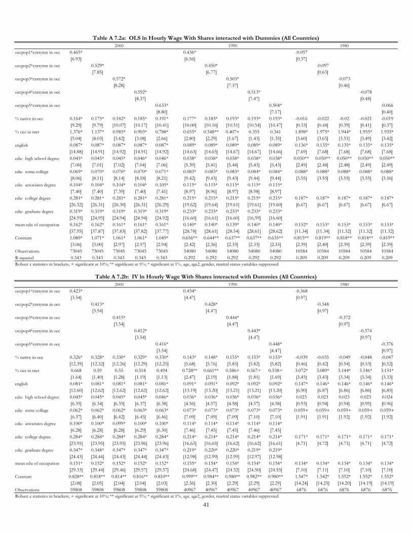
occpop1*cntrymn in occ 0.465* 0.436* -0.057

[6.93] [6.56] [0.37]

occpop2*cntrymn in occ 0.529* 0.450* -0.097

[7.85] [6.77] [0.63]

occpop3*cntrymn in occ 0.572* 0.503* -0.073

[8.28] [7.37] [0.46]

occpop4*cntrymn in occ 0.592* 0.513* -0.078

[8.37] [7.47] [0.48]

occpop5*cntrymn in occ 0.633* 0.504* -0.066

[8.80] [7.17] [0.40]

% native in occ 0.164* 0.175* 0.182* 0.185* 0.191* 0.177* 0.183* 0.193* 0.193* 0.193* -0.016 -0.022 -0.02 -0.021 -0.019

[9.29] [9.79] [10.07] [10.17] [10.41] [10.00] [10.16] [10.51] [10.54] [10.47] [0.33] [0.44] [0.39] [0.41] [0.37]

% occ in met 1.376* 1.137* 0.985* 0.903* 0.788* 0.655* 0.548** 0.407+ 0.355 0.341 1.898* 1.975* 1.944* 1.955* 1.935*

[5.04] [4.03] [3.42] [3.08] [2.66] [2.80] [2.29] [1.67] [1.43] [1.35] [3.60] [3.65] [3.51] [3.49] [3.42]

english 0.087* 0.087* 0.087* 0.087* 0.087* 0.089* 0.089* 0.089* 0.089* 0.089* 0.136* 0.135* 0.135* 0.135* 0.135*

[14.88] [14.91] [14.92] [14.91] [14.92] [14.63] [14.65] [14.67] [14.67] [14.66] [7.69] [7.68] [7.68] [7.68] [7.68]

edu: high school degree 0.045* 0.045* 0.045* 0.046* 0.046* 0.038* 0.038* 0.038* 0.038* 0.038* 0.050** 0.050** 0.050** 0.050** 0.050**

[7.00] [7.01] [7.02] [7.04] [7.06] [5.39] [5.41] [5.44] [5.43] [5.43] [2.49] [2.48] [2.48] [2.49] [2.49]

edu: some college 0.069* 0.070* 0.070* 0.070* 0.071* 0.083* 0.083* 0.083* 0.084* 0.084* 0.088* 0.088* 0.088* 0.088* 0.088*

[8.06] [8.11] [8.14] [8.18] [8.21] [9.42] [9.43] [9.43] [9.44] [9.44] [3.55] [3.55] [3.55] [3.55] [3.56]

edu: associates degree 0.104* 0.104* 0.104* 0.104* 0.105* 0.115* 0.115* 0.115* 0.115* 0.115*

[7.40] [7.40] [7.39] [7.40] [7.41] [8.97] [8.96] [8.97] [8.98] [8.97]

edu: college degree 0.281* 0.281* 0.281* 0.281* 0.281* 0.215* 0.215* 0.215* 0.215* 0.215* 0.187* 0.187* 0.187* 0.187* 0.187*

[26.32] [26.31] [26.30] [26.31] [26.29] [19.62] [19.64] [19.61] [19.61] [19.60] [6.67] [6.67] [6.67] [6.67] [6.67]

edu: graduate degree 0.319* 0.319* 0.319* 0.319* 0.319* 0.233* 0.233* 0.233* 0.233* 0.233*

[24.95] [24.95] [24.94] [24.94] [24.92] [16.60] [16.61] [16.60] [16.59] [16.60]

mean edu of occupation 0.162* 0.162* 0.161* 0.161* 0.161* 0.140* 0.140* 0.139* 0.140* 0.140* 0.152* 0.153* 0.153* 0.153* 0.153*

[37.95] [37.87] [37.83] [37.82] [37.77] [28.78] [28.61] [28.54] [28.61] [28.62] [11.34] [11.34] [11.32] [11.32] [11.32]

Constant 1.089* 1.071* 1.061* 1.061* 1.049* 0.656** 0.644** 0.637** 0.637** 0.635** 0.815** 0.819** 0.818** 0.818** 0.819**

[3.06] [3.00] [2.97] [2.97] [2.94] [2.42] [2.36] [2.33] [2.33] [2.33] [2.39] [2.40] [2.39] [2.39] [2.39]

Observations 73045 73045 73045 73045 73045 54080 54080 54080 54080 54080 10584 10584 10584 10584 10584

R-squared 0.343 0.343 0.343 0.343 0.343 0.292 0.292 0.292 0.292 0.292 0.209 0.209 0.209 0.209 0.209

occpop1*cntrymn in occ 0.423* 0.434* -0.368

[3.54] [4.47] [0.97]

occpop2*cntrymn in occ 0.413* 0.428* -0.348

[3.54] [4.47] [0.97]

occpop3*cntrymn in occ 0.415* 0.444* -0.372

[3.54] [4.47] [0.97]

occpop4*cntrymn in occ 0.412* 0.443* -0.374

[3.54] [4.47] [0.97]

occpop5*cntrymn in occ 0.416* 0.448* -0.376

[3.54] [4.47] [0.97]

% native in occ 0.326* 0.328* 0.330* 0.329* 0.330* 0.143* 0.148* 0.155* 0.153* 0.153* -0.039 -0.035 -0.049 -0.048 -0.047

[12.39] [12.32] [12.26] [12.29] [12.25] [5.68] [5.76] [5.85] [5.82] [5.82] [0.46] [0.42] [0.54] [0.53] [0.52]

% occ in met 0.668 0.59 0.55 0.518 0.494 0.728** 0.661** 0.586+ 0.567+ 0.538+ 3.072* 3.089* 3.144* 3.146* 3.151*

[1.64] [1.40] [1.28] [1.19] [1.13] [2.47] [2.19] [1.88] [1.81] [1.69] [3.45] [3.43] [3.34] [3.34] [3.33]

english 0.081* 0.081* 0.081* 0.081* 0.081* 0.091* 0.091* 0.092* 0.092* 0.092* 0.147* 0.146* 0.146* 0.146* 0.146*

[12.60] [12.62] [12.62] [12.62] [12.62] [13.19] [13.20] [13.21] [13.21] [13.20] [6.90] [6.87] [6.86] [6.86] [6.85]

edu: high school degree 0.045* 0.045* 0.045* 0.045* 0.046* 0.036* 0.036* 0.036* 0.036* 0.036* 0.023 0.023 0.023 0.023 0.024

[6.35] [6.34] [6.35] [6.37] [6.38] [4.56] [4.57] [4.58] [4.57] [4.58] [0.93] [0.94] [0.94] [0.95] [0.96]

edu: some college 0.062* 0.062* 0.062* 0.063* 0.063* 0.073* 0.073* 0.073* 0.073* 0.073* 0.059+ 0.059+ 0.059+ 0.059+ 0.059+

[6.37] [6.40] [6.42] [6.45] [6.46] [7.09] [7.09] [7.09] [7.10] [7.10] [1.91] [1.91] [1.92] [1.92] [1.92]

edu: associates degree 0.100* 0.100* 0.099* 0.100* 0.100* 0.114* 0.114* 0.114* 0.114* 0.114*

[6.28] [6.28] [6.28] [6.29] [6.30] [7.46] [7.45] [7.45] [7.46] [7.45]

edu: college degree 0.284* 0.284* 0.284* 0.284* 0.284* 0.214* 0.214* 0.214* 0.214* 0.214* 0.171* 0.171* 0.171* 0.171* 0.171*

[23.95] [23.95] [23.95] [23.96] [23.96] [16.63] [16.65] [16.62] [16.62] [16.61] [4.71] [4.72] [4.71] [4.71] [4.72]

edu: graduate degree 0.347* 0.348* 0.347* 0.347* 0.347* 0.219* 0.220* 0.220* 0.219* 0.219*

[24.43] [24.44] [24.43] [24.44] [24.43] [12.98] [12.99] [12.99] [12.97] [12.98]

mean edu of occupation 0.151* 0.152* 0.152* 0.152* 0.152* 0.155* 0.154* 0.154* 0.154* 0.154* 0.134* 0.134* 0.134* 0.134* 0.134*

[29.33] [29.44] [29.46] [29.57] [29.57] [24.68] [24.47] [24.32] [24.50] [24.55] [7.10] [7.11] [7.10] [7.10] [7.10]

Constant 0.828** 0.818** 0.814** 0.816** 0.810** 0.999** 0.984** 0.980** 0.982** 0.980** 1.547* 1.542* 1.552* 1.552* 1.552*

[2.08] [2.05] [2.04] [2.04] [2.03] [2.36] [2.30] [2.29] [2.29] [2.29] [14.24] [14.25] [14.20] [14.19] [14.19]

Observations 59808 59808 59808 59808 59808 40967 40967 40967 40967 40967 6876 6876 6876 6876 6876

Robust z statistics in brackets, + significant at 10%; ** significant at 5%; * significant at 1%, age, age2, gender, marital status variables suppressed

Robust z statistics in brackets, + significant at 10%; ** significant at 5%; * significant at 1%, age, age2, gender, marital status variables suppressed

Table A 7.2b: IV ln Hourly Wage With Shares interacted with Dummies (All Countries)

2000 1990 1980

Table A 7.2a: OLS ln Hourly Wage With Shares interacted with Dummies (All Countries)

2000 1990 1980

41

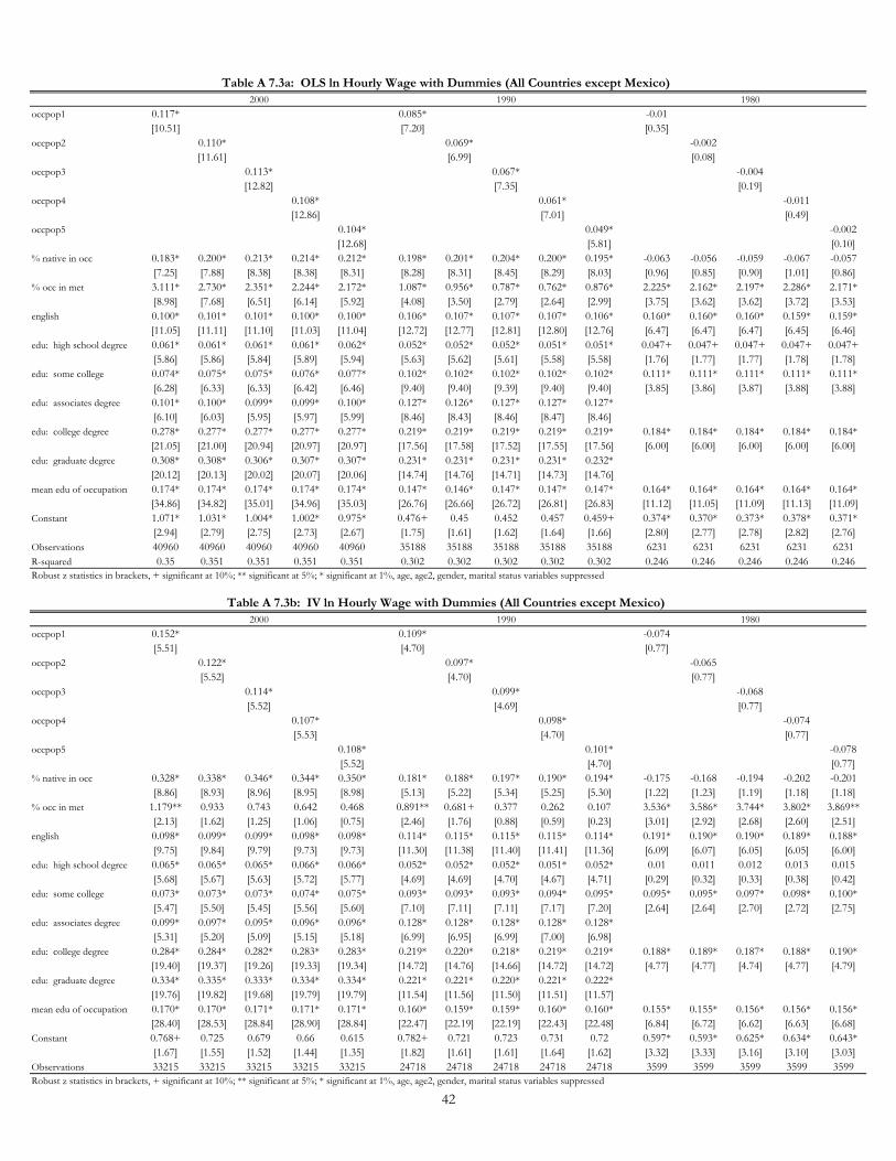
occpop1 0.117* 0.085* -0.01

[10.51] [7.20] [0.35]

occpop2 0.110* 0.069* -0.002

[11.61] [6.99] [0.08]

occpop3 0.113* 0.067* -0.004

[12.82] [7.35] [0.19]

occpop4 0.108* 0.061* -0.011

[12.86] [7.01] [0.49]

occpop5 0.104* 0.049* -0.002

[12.68] [5.81] [0.10]

% native in occ 0.183* 0.200* 0.213* 0.214* 0.212* 0.198* 0.201* 0.204* 0.200* 0.195* -0.063 -0.056 -0.059 -0.067 -0.057

[7.25] [7.88] [8.38] [8.38] [8.31] [8.28] [8.31] [8.45] [8.29] [8.03] [0.96] [0.85] [0.90] [1.01] [0.86]

% occ in met 3.111* 2.730* 2.351* 2.244* 2.172* 1.087* 0.956* 0.787* 0.762* 0.876* 2.225* 2.162* 2.197* 2.286* 2.171*

[8.98] [7.68] [6.51] [6.14] [5.92] [4.08] [3.50] [2.79] [2.64] [2.99] [3.75] [3.62] [3.62] [3.72] [3.53]

english 0.100* 0.101* 0.101* 0.100* 0.100* 0.106* 0.107* 0.107* 0.107* 0.106* 0.160* 0.160* 0.160* 0.159* 0.159*

[11.05] [11.11] [11.10] [11.03] [11.04] [12.72] [12.77] [12.81] [12.80] [12.76] [6.47] [6.47] [6.47] [6.45] [6.46]

edu: high school degree 0.061* 0.061* 0.061* 0.061* 0.062* 0.052* 0.052* 0.052* 0.051* 0.051* 0.047+ 0.047+ 0.047+ 0.047+ 0.047+

[5.86] [5.86] [5.84] [5.89] [5.94] [5.63] [5.62] [5.61] [5.58] [5.58] [1.76] [1.77] [1.77] [1.78] [1.78]

edu: some college 0.074* 0.075* 0.075* 0.076* 0.077* 0.102* 0.102* 0.102* 0.102* 0.102* 0.111* 0.111* 0.111* 0.111* 0.111*

[6.28] [6.33] [6.33] [6.42] [6.46] [9.40] [9.40] [9.39] [9.40] [9.40] [3.85] [3.86] [3.87] [3.88] [3.88]

edu: associates degree 0.101* 0.100* 0.099* 0.099* 0.100* 0.127* 0.126* 0.127* 0.127* 0.127*

[6.10] [6.03] [5.95] [5.97] [5.99] [8.46] [8.43] [8.46] [8.47] [8.46]

edu: college degree 0.278* 0.277* 0.277* 0.277* 0.277* 0.219* 0.219* 0.219* 0.219* 0.219* 0.184* 0.184* 0.184* 0.184* 0.184*

[21.05] [21.00] [20.94] [20.97] [20.97] [17.56] [17.58] [17.52] [17.55] [17.56] [6.00] [6.00] [6.00] [6.00] [6.00]

edu: graduate degree 0.308* 0.308* 0.306* 0.307* 0.307* 0.231* 0.231* 0.231* 0.231* 0.232*

[20.12] [20.13] [20.02] [20.07] [20.06] [14.74] [14.76] [14.71] [14.73] [14.76]

mean edu of occupation 0.174* 0.174* 0.174* 0.174* 0.174* 0.147* 0.146* 0.147* 0.147* 0.147* 0.164* 0.164* 0.164* 0.164* 0.164*

[34.86] [34.82] [35.01] [34.96] [35.03] [26.76] [26.66] [26.72] [26.81] [26.83] [11.12] [11.05] [11.09] [11.13] [11.09]

Constant 1.071* 1.031* 1.004* 1.002* 0.975* 0.476+ 0.45 0.452 0.457 0.459+ 0.374* 0.370* 0.373* 0.378* 0.371*

[2.94] [2.79] [2.75] [2.73] [2.67] [1.75] [1.61] [1.62] [1.64] [1.66] [2.80] [2.77] [2.78] [2.82] [2.76]

Observations 40960 40960 40960 40960 40960 35188 35188 35188 35188 35188 6231 6231 6231 6231 6231

R-squared 0.35 0.351 0.351 0.351 0.351 0.302 0.302 0.302 0.302 0.302 0.246 0.246 0.246 0.246 0.246

occpop1 0.152* 0.109* -0.074

[5.51] [4.70] [0.77]

occpop2 0.122* 0.097* -0.065

[5.52] [4.70] [0.77]

occpop3 0.114* 0.099* -0.068

[5.52] [4.69] [0.77]

occpop4 0.107* 0.098* -0.074

[5.53] [4.70] [0.77]

occpop5 0.108* 0.101* -0.078

[5.52] [4.70] [0.77]

% native in occ 0.328* 0.338* 0.346* 0.344* 0.350* 0.181* 0.188* 0.197* 0.190* 0.194* -0.175 -0.168 -0.194 -0.202 -0.201

[8.86] [8.93] [8.96] [8.95] [8.98] [5.13] [5.22] [5.34] [5.25] [5.30] [1.22] [1.23] [1.19] [1.18] [1.18]

% occ in met 1.179** 0.933 0.743 0.642 0.468 0.891** 0.681+ 0.377 0.262 0.107 3.536* 3.586* 3.744* 3.802* 3.869**

[2.13] [1.62] [1.25] [1.06] [0.75] [2.46] [1.76] [0.88] [0.59] [0.23] [3.01] [2.92] [2.68] [2.60] [2.51]

english 0.098* 0.099* 0.099* 0.098* 0.098* 0.114* 0.115* 0.115* 0.115* 0.114* 0.191* 0.190* 0.190* 0.189* 0.188*

[9.75] [9.84] [9.79] [9.73] [9.73] [11.30] [11.38] [11.40] [11.41] [11.36] [6.09] [6.07] [6.05] [6.05] [6.00]

edu: high school degree 0.065* 0.065* 0.065* 0.066* 0.066* 0.052* 0.052* 0.052* 0.051* 0.052* 0.01 0.011 0.012 0.013 0.015

[5.68] [5.67] [5.63] [5.72] [5.77] [4.69] [4.69] [4.70] [4.67] [4.71] [0.29] [0.32] [0.33] [0.38] [0.42]

edu: some college 0.073* 0.073* 0.073* 0.074* 0.075* 0.093* 0.093* 0.093* 0.094* 0.095* 0.095* 0.095* 0.097* 0.098* 0.100*

[5.47] [5.50] [5.45] [5.56] [5.60] [7.10] [7.11] [7.11] [7.17] [7.20] [2.64] [2.64] [2.70] [2.72] [2.75]

edu: associates degree 0.099* 0.097* 0.095* 0.096* 0.096* 0.128* 0.128* 0.128* 0.128* 0.128*

[5.31] [5.20] [5.09] [5.15] [5.18] [6.99] [6.95] [6.99] [7.00] [6.98]

edu: college degree 0.284* 0.284* 0.282* 0.283* 0.283* 0.219* 0.220* 0.218* 0.219* 0.219* 0.188* 0.189* 0.187* 0.188* 0.190*

[19.40] [19.37] [19.26] [19.33] [19.34] [14.72] [14.76] [14.66] [14.72] [14.72] [4.77] [4.77] [4.74] [4.77] [4.79]

edu: graduate degree 0.334* 0.335* 0.333* 0.334* 0.334* 0.221* 0.221* 0.220* 0.221* 0.222*

[19.76] [19.82] [19.68] [19.79] [19.79] [11.54] [11.56] [11.50] [11.51] [11.57]

mean edu of occupation 0.170* 0.170* 0.171* 0.171* 0.171* 0.160* 0.159* 0.159* 0.160* 0.160* 0.155* 0.155* 0.156* 0.156* 0.156*

[28.40] [28.53] [28.84] [28.90] [28.84] [22.47] [22.19] [22.19] [22.43] [22.48] [6.84] [6.72] [6.62] [6.63] [6.68]

Constant 0.768+ 0.725 0.679 0.66 0.615 0.782+ 0.721 0.723 0.731 0.72 0.597* 0.593* 0.625* 0.634* 0.643*

[1.67] [1.55] [1.52] [1.44] [1.35] [1.82] [1.61] [1.61] [1.64] [1.62] [3.32] [3.33] [3.16] [3.10] [3.03]

Observations 33215 33215 33215 33215 33215 24718 24718 24718 24718 24718 3599 3599 3599 3599 3599

Robust z statistics in brackets, + significant at 10%; ** significant at 5%; * significant at 1%, age, age2, gender, marital status variables suppressed

Robust z statistics in brackets, + significant at 10%; ** significant at 5%; * significant at 1%, age, age2, gender, marital status variables suppressed

Table A 7.3b: IV ln Hourly Wage with Dummies (All Countries except Mexico)

2000 1990 1980

Table A 7.3a: OLS ln Hourly Wage with Dummies (All Countries except Mexico)

2000 1990 1980

42

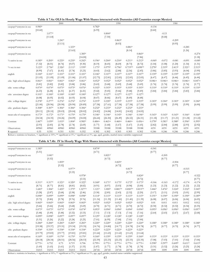
occpop1*cntrymn in occ 0.985* 0.782* -0.134

[10.60] [6.95] [0.60]

occpop2*cntrymn in occ 1.077* 0.804* -0.15

[11.64] [7.50] [0.68]

occpop3*cntrymn in occ 1.241* 0.863* -0.209

[13.11] [8.03] [0.95]

occpop4*cntrymn in occ 1.323* 0.881* -0.285

[13.65] [8.14] [1.26]

occpop5*cntrymn in occ 1.385* 0.865* -0.274

[14.00] [7.86] [1.18]

% native in occ 0.185* 0.205* 0.225* 0.235* 0.242* 0.196* 0.204* 0.210* 0.211* 0.212* -0.069 -0.072 -0.081 -0.091 -0.089

[7.32] [8.01] [8.74] [9.07] [9.30] [8.19] [8.45] [8.69] [8.73] [8.72] [1.04] [1.08] [1.20] [1.34] [1.31]

% occ in met 3.123* 2.736* 2.326* 2.111* 1.939* 1.175* 0.979* 0.796* 0.719** 0.698** 2.278* 2.319* 2.413* 2.521* 2.513*

[8.99] [7.67] [6.41] [5.74] [5.23] [4.43] [3.62] [2.88] [2.56] [2.45] [3.86] [3.85] [3.93] [4.04] [3.99]

english 0.100* 0.101* 0.101* 0.101* 0.101* 0.106* 0.107* 0.107* 0.107* 0.107* 0.159* 0.159* 0.159* 0.159* 0.159*

[11.05] [11.09] [11.09] [11.06] [11.07] [12.75] [12.81] [12.83] [12.83] [12.83] [6.47] [6.47] [6.46] [6.45] [6.44]

edu: high school degree 0.061* 0.061* 0.061* 0.061* 0.061* 0.052* 0.052* 0.052* 0.052* 0.052* 0.046+ 0.046+ 0.046+ 0.046+ 0.047+

[5.81] [5.82] [5.82] [5.84] [5.86] [5.65] [5.68] [5.69] [5.68] [5.69] [1.76] [1.76] [1.76] [1.76] [1.77]

edu: some college 0.074* 0.074* 0.075* 0.075* 0.076* 0.102* 0.103* 0.103* 0.103* 0.103* 0.110* 0.110* 0.110* 0.110* 0.110*

[6.23] [6.28] [6.31] [6.37] [6.41] [9.42] [9.45] [9.46] [9.48] [9.49] [3.84] [3.84] [3.84] [3.83] [3.84]

edu: associates degree 0.101* 0.100* 0.100* 0.100* 0.100* 0.127* 0.127* 0.127* 0.127* 0.127*

[6.08] [6.05] [6.02] [6.03] [6.04] [8.47] [8.46] [8.47] [8.49] [8.48]

edu: college degree 0.278* 0.277* 0.276* 0.276* 0.276* 0.219* 0.220* 0.219* 0.219* 0.219* 0.183* 0.184* 0.183* 0.183* 0.184*

[21.00] [20.96] [20.90] [20.90] [20.89] [17.58] [17.61] [17.58] [17.58] [17.58] [5.99] [5.99] [5.99] [5.99] [6.00]

edu: graduate degree 0.308* 0.307* 0.306* 0.306* 0.306* 0.232* 0.233* 0.232* 0.232* 0.233*

[20.11] [20.10] [20.03] [20.04] [20.02] [14.82] [14.84] [14.81] [14.82] [14.83]

mean edu of occupation 0.173* 0.172* 0.171* 0.170* 0.170* 0.146* 0.146* 0.145* 0.146* 0.146* 0.165* 0.165* 0.165* 0.166* 0.166*

[34.54] [34.35] [34.26] [34.09] [34.00] [26.64] [26.50] [26.49] [26.52] [26.51] [11.18] [11.17] [11.21] [11.24] [11.22]

Constant 1.067* 1.039* 1.015* 1.004* 0.985* 0.484+ 0.463+ 0.460+ 0.460+ 0.456+ 0.378* 0.381* 0.388* 0.396* 0.395*

[2.93] [2.83] [2.78] [2.74] [2.69] [1.77] [1.68] [1.67] [1.67] [1.65] [2.82] [2.84] [2.88] [2.93] [2.92]

Observations 40960 40960 40960 40960 40960 35188 35188 35188 35188 35188 6231 6231 6231 6231 6231

R-squared 0.35 0.351 0.351 0.351 0.352 0.302 0.302 0.303 0.303 0.302 0.246 0.246 0.246 0.246 0.246

occpop1*cntrymn in occ 1.185* 0.874* -0.541

[5.51] [4.71] [0.77]

occpop2*cntrymn in occ 1.041* 0.821* -0.505

[5.52] [4.72] [0.77]

occpop3*cntrymn in occ 1.005* 0.825* -0.504

[5.52] [4.72] [0.77]

occpop4*cntrymn in occ 0.977* 0.817* -0.515

[5.53] [4.72] [0.77]

occpop5*cntrymn in occ 0.978* 0.824* -0.522

[5.53] [4.72] [0.77]

% native in occ 0.311* 0.317* 0.321* 0.320* 0.322* 0.168* 0.171* 0.175* 0.172* 0.173* -0.166 -0.163 -0.172 -0.174 -0.174

[8.71] [8.77] [8.81] [8.81] [8.82] [4.91] [4.97] [5.03] [4.98] [5.00] [1.23] [1.23] [1.22] [1.22] [1.22]

% occ in met 1.683* 1.506* 1.425* 1.379* 1.327** 1.121* 1.000* 0.881** 0.850** 0.815** 3.446* 3.476* 3.524* 3.532* 3.545*

[3.28] [2.87] [2.68] [2.58] [2.46] [3.30] [2.85] [2.43] [2.32] [2.20] [3.17] [3.11] [3.03] [3.01] [2.99]

english 0.098* 0.099* 0.099* 0.098* 0.098* 0.114* 0.115* 0.115* 0.115* 0.115* 0.191* 0.190* 0.190* 0.190* 0.189*

[9.75] [9.80] [9.78] [9.76] [9.76] [11.34] [11.39] [11.40] [11.40] [11.39] [6.08] [6.07] [6.06] [6.06] [6.05]

edu: high school degree 0.065* 0.065* 0.065* 0.065* 0.065* 0.052* 0.052* 0.052* 0.052* 0.052* 0.01 0.011 0.011 0.012 0.012

[5.66] [5.66] [5.64] [5.68] [5.69] [4.70] [4.71] [4.71] [4.70] [4.72] [0.30] [0.32] [0.32] [0.34] [0.35]

edu: some college 0.073* 0.073* 0.073* 0.074* 0.074* 0.093* 0.094* 0.094* 0.094* 0.094* 0.095* 0.096* 0.096* 0.096* 0.097*

[5.48] [5.49] [5.48] [5.52] [5.53] [7.11] [7.13] [7.13] [7.16] [7.16] [2.64] [2.65] [2.67] [2.67] [2.68]

edu: associates degree 0.099* 0.098* 0.097* 0.097* 0.097* 0.129* 0.128* 0.128* 0.128* 0.128*

[5.31] [5.26] [5.22] [5.24] [5.25] [7.01] [6.99] [7.00] [7.01] [7.00]

edu: college degree 0.284* 0.284* 0.283* 0.283* 0.283* 0.220* 0.220* 0.220* 0.220* 0.220* 0.188* 0.188* 0.188* 0.188* 0.188*

[19.38] [19.37] [19.31] [19.34] [19.35] [14.76] [14.80] [14.77] [14.78] [14.78] [4.77] [4.77] [4.75] [4.76] [4.77]

edu: graduate degree 0.334* 0.335* 0.334* 0.334* 0.334* 0.223* 0.223* 0.223* 0.223* 0.223*

[19.79] [19.83] [19.77] [19.81] [19.81] [11.64] [11.65] [11.62] [11.63] [11.64]

mean edu of occupation 0.169* 0.169* 0.170* 0.170* 0.170* 0.160* 0.159* 0.159* 0.159* 0.160* 0.153* 0.153* 0.153* 0.153* 0.153*

[28.18] [28.34] [28.51] [28.56] [28.53] [22.39] [22.23] [22.23] [22.33] [22.35] [7.08] [7.03] [7.01] [7.02] [7.04]

Constant 0.775+ 0.752 0.73 0.719 0.706 0.799+ 0.772+ 0.773+ 0.775+ 0.773+ 0.598* 0.597* 0.609* 0.611* 0.613*

[1.69] [1.63] [1.61] [1.57] [1.55] [1.87] [1.77] [1.78] [1.78] [1.78] [3.31] [3.32] [3.26] [3.25] [3.24]

Observations 33215 33215 33215 33215 33215 24718 24718 24718 24718 24718 3599 3599 3599 3599 3599

Robust z statistics in brackets, + significant at 10%; ** significant at 5%; * significant at 1%, age, age2, gender, marital status variables suppressed

Robust z statistics in brackets, + significant at 10%; ** significant at 5%; * significant at 1%, age, age2, gender, marital status variables suppressed

Table A 7.4b: IV ln Hourly Wage With Shares interacted with Dummies (All Countries except Mexico)

2000 1990 1980

Table A 7.4a: OLS ln Hourly Wage With Shares interacted with Dummies (All Countries except Mexico)

2000 1990 1980

43

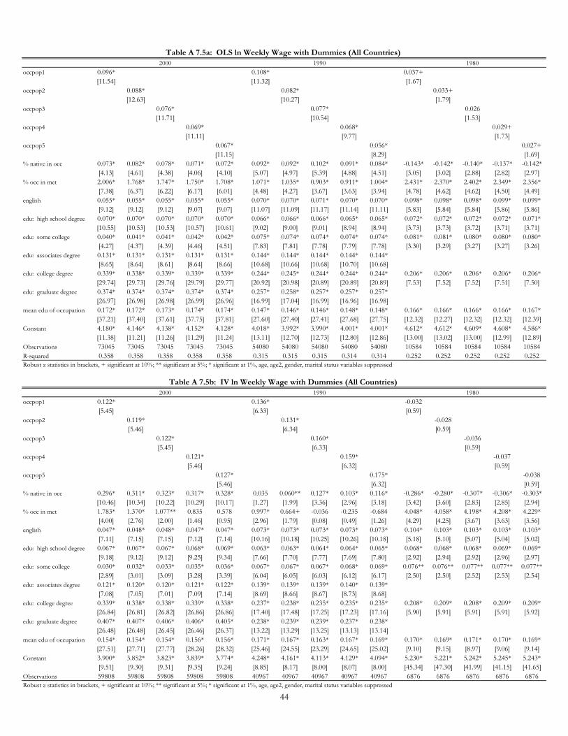
occpop1 0.096* 0.108* 0.037+

[11.54] [11.32] [1.67]

occpop2 0.088* 0.082* 0.033+

[12.63] [10.27] [1.79]

occpop3 0.076* 0.077* 0.026

[11.71] [10.54] [1.53]

occpop4 0.069* 0.068* 0.029+

[11.11] [9.77] [1.73]

occpop5 0.067* 0.056* 0.027+

[11.15] [8.29] [1.69]

% native in occ 0.073* 0.082* 0.078* 0.071* 0.072* 0.092* 0.092* 0.102* 0.091* 0.084* -0.143* -0.142* -0.140* -0.137* -0.142*

[4.13] [4.61] [4.38] [4.06] [4.10] [5.07] [4.97] [5.39] [4.88] [4.51] [3.05] [3.02] [2.88] [2.82] [2.97]

% occ in met 2.006* 1.768* 1.747* 1.750* 1.708* 1.071* 1.035* 0.903* 0.911* 1.004* 2.431* 2.370* 2.402* 2.349* 2.356*

[7.38] [6.37] [6.22] [6.17] [6.01] [4.48] [4.27] [3.67] [3.63] [3.94] [4.78] [4.62] [4.62] [4.50] [4.49]

english 0.055* 0.055* 0.055* 0.055* 0.055* 0.070* 0.070* 0.071* 0.070* 0.070* 0.098* 0.098* 0.098* 0.099* 0.099*

[9.12] [9.12] [9.12] [9.07] [9.07] [11.07] [11.09] [11.17] [11.14] [11.11] [5.83] [5.84] [5.84] [5.86] [5.86]

edu: high school degree 0.070* 0.070* 0.070* 0.070* 0.070* 0.066* 0.066* 0.066* 0.065* 0.065* 0.072* 0.072* 0.072* 0.072* 0.071*

[10.55] [10.53] [10.53] [10.57] [10.61] [9.02] [9.00] [9.01] [8.94] [8.94] [3.73] [3.73] [3.72] [3.71] [3.71]

edu: some college 0.040* 0.041* 0.041* 0.042* 0.042* 0.075* 0.074* 0.074* 0.074* 0.074* 0.081* 0.081* 0.080* 0.080* 0.080*

[4.27] [4.37] [4.39] [4.46] [4.51] [7.83] [7.81] [7.78] [7.79] [7.78] [3.30] [3.29] [3.27] [3.27] [3.26]

edu: associates degree 0.131* 0.131* 0.131* 0.131* 0.131* 0.144* 0.144* 0.144* 0.144* 0.144*

[8.65] [8.64] [8.61] [8.64] [8.66] [10.68] [10.66] [10.68] [10.70] [10.68]

edu: college degree 0.339* 0.338* 0.339* 0.339* 0.339* 0.244* 0.245* 0.244* 0.244* 0.244* 0.206* 0.206* 0.206* 0.206* 0.206*

[29.74] [29.73] [29.76] [29.79] [29.77] [20.92] [20.98] [20.89] [20.89] [20.89] [7.53] [7.52] [7.52] [7.51] [7.50]

edu: graduate degree 0.374* 0.374* 0.374* 0.374* 0.374* 0.257* 0.258* 0.257* 0.257* 0.257*

[26.97] [26.98] [26.98] [26.99] [26.96] [16.99] [17.04] [16.99] [16.96] [16.98]

mean edu of occupation 0.172* 0.172* 0.173* 0.174* 0.174* 0.147* 0.146* 0.146* 0.148* 0.148* 0.166* 0.166* 0.166* 0.166* 0.167*

[37.21] [37.40] [37.61] [37.75] [37.81] [27.60] [27.40] [27.41] [27.68] [27.75] [12.32] [12.27] [12.32] [12.32] [12.39]

Constant 4.180* 4.146* 4.138* 4.152* 4.128* 4.018* 3.992* 3.990* 4.001* 4.001* 4.612* 4.612* 4.609* 4.608* 4.586*

[11.38] [11.21] [11.26] [11.29] [11.24] [13.11] [12.70] [12.73] [12.80] [12.86] [13.00] [13.02] [13.00] [12.99] [12.89]

Observations 73045 73045 73045 73045 73045 54080 54080 54080 54080 54080 10584 10584 10584 10584 10584

R-squared 0.358 0.358 0.358 0.358 0.358 0.315 0.315 0.315 0.314 0.314 0.252 0.252 0.252 0.252 0.252

occpop1 0.122* 0.136* -0.032

[5.45] [6.33] [0.59]

occpop2 0.119* 0.131* -0.028

[5.46] [6.34] [0.59]

occpop3 0.122* 0.160* -0.036

[5.45] [6.33] [0.59]

occpop4 0.121* 0.159* -0.037

[5.46] [6.32] [0.59]

occpop5 0.127* 0.175* -0.038

[5.46] [6.32] [0.59]

% native in occ 0.296* 0.311* 0.323* 0.317* 0.328* 0.035 0.060** 0.127* 0.103* 0.116* -0.286* -0.280* -0.307* -0.306* -0.303*

[10.46] [10.34] [10.22] [10.29] [10.17] [1.27] [1.99] [3.36] [2.96] [3.18] [3.42] [3.60] [2.83] [2.85] [2.94]

% occ in met 1.783* 1.370* 1.077** 0.835 0.578 0.997* 0.664+ -0.036 -0.235 -0.684 4.048* 4.058* 4.198* 4.208* 4.229*

[4.00] [2.76] [2.00] [1.46] [0.95] [2.96] [1.79] [0.08] [0.49] [1.26] [4.29] [4.25] [3.67] [3.63] [3.56]

english 0.047* 0.048* 0.048* 0.047* 0.047* 0.073* 0.073* 0.073* 0.073* 0.073* 0.104* 0.103* 0.103* 0.103* 0.103*

[7.11] [7.15] [7.15] [7.12] [7.14] [10.16] [10.18] [10.25] [10.26] [10.18] [5.18] [5.10] [5.07] [5.04] [5.02]

edu: high school degree 0.067* 0.067* 0.067* 0.068* 0.069* 0.063* 0.063* 0.064* 0.064* 0.065* 0.068* 0.068* 0.068* 0.069* 0.069*

[9.18] [9.12] [9.12] [9.25] [9.34] [7.66] [7.70] [7.77] [7.69] [7.80] [2.92] [2.94] [2.92] [2.96] [2.97]

edu: some college 0.030* 0.032* 0.033* 0.035* 0.036* 0.067* 0.067* 0.067* 0.068* 0.069* 0.076** 0.076** 0.077** 0.077** 0.077**

[2.89] [3.01] [3.09] [3.28] [3.39] [6.04] [6.05] [6.03] [6.12] [6.17] [2.50] [2.50] [2.52] [2.53] [2.54]

edu: associates degree 0.121* 0.120* 0.120* 0.121* 0.122* 0.139* 0.139* 0.139* 0.140* 0.139*

[7.08] [7.05] [7.01] [7.09] [7.14] [8.69] [8.66] [8.67] [8.73] [8.68]

edu: college degree 0.339* 0.338* 0.338* 0.339* 0.338* 0.237* 0.238* 0.235* 0.235* 0.235* 0.208* 0.209* 0.208* 0.209* 0.209*

[26.84] [26.81] [26.82] [26.86] [26.86] [17.40] [17.48] [17.25] [17.23] [17.16] [5.90] [5.91] [5.91] [5.91] [5.92]

edu: graduate degree 0.407* 0.407* 0.406* 0.406* 0.405* 0.238* 0.239* 0.239* 0.237* 0.238*

[26.48] [26.48] [26.45] [26.46] [26.37] [13.22] [13.29] [13.25] [13.13] [13.14]

mean edu of occupation 0.154* 0.154* 0.154* 0.156* 0.156* 0.171* 0.167* 0.163* 0.167* 0.169* 0.170* 0.169* 0.171* 0.170* 0.169*

[27.51] [27.71] [27.77] [28.26] [28.32] [25.46] [24.55] [23.29] [24.65] [25.02] [9.10] [9.15] [8.97] [9.06] [9.14]

Constant 3.900* 3.852* 3.823* 3.839* 3.774* 4.248* 4.161* 4.113* 4.129* 4.094* 5.230* 5.221* 5.242* 5.245* 5.243*

[9.51] [9.30] [9.31] [9.35] [9.24] [8.85] [8.17] [8.00] [8.07] [8.00] [45.34] [47.30] [41.99] [41.15] [41.65]

Observations 59808 59808 59808 59808 59808 40967 40967 40967 40967 40967 6876 6876 6876 6876 6876

Robust z statistics in brackets, + significant at 10%; ** significant at 5%; * significant at 1%, age, age2, gender, marital status variables suppressed

Robust z statistics in brackets, + significant at 10%; ** significant at 5%; * significant at 1%, age, age2, gender, marital status variables suppressed

Table A 7.5b: IV ln Weekly Wage with Dummies (All Countries)

2000 1990 1980

Table A 7.5a: OLS ln Weekly Wage with Dummies (All Countries)

2000 1990 1980

44

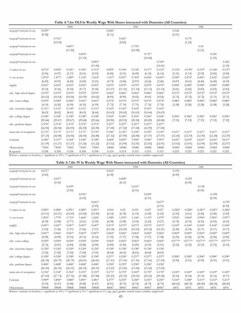
occpop1*cntrymn in occ 0.639* 0.606* 0.144

[9.28] [9.11] [1.01]

occpop2*cntrymn in occ 0.761* 0.661* 0.174

[10.94] [9.85] [1.22]

occpop3*cntrymn in occ 0.807* 0.735* 0.18

[11.30] [10.58] [1.21]

occpop4*cntrymn in occ 0.845* 0.747* 0.184

[11.55] [10.68] [1.23]

occpop5*cntrymn in occ 0.893* 0.745* 0.182

[11.96] [10.41] [1.19]

% native in occ 0.072* 0.092* 0.101* 0.106* 0.113* 0.092* 0.104* 0.118* 0.117* 0.119* -0.155* -0.150* -0.147* -0.146* -0.147*

[3.96] [4.97] [5.37] [5.61] [5.93] [4.96] [5.51] [6.09] [6.10] [6.14] [3.31] [3.15] [2.99] [2.96] [2.98]

% occ in met 1.872* 1.477* 1.289* 1.152* 1.014* 1.167* 0.967* 0.765* 0.694* 0.654** 2.550* 2.472* 2.445* 2.432* 2.432*

[6.45] [4.91] [4.20] [3.69] [3.21] [4.73] [3.84] [2.97] [2.66] [2.46] [4.87] [4.61] [4.46] [4.40] [4.35]

english 0.055* 0.055* 0.055* 0.055* 0.055* 0.070* 0.070* 0.070* 0.070* 0.070* 0.098* 0.098* 0.098* 0.098* 0.098*

[9.12] [9.16] [9.18] [9.17] [9.18] [11.07] [11.10] [11.14] [11.13] [11.12] [5.81] [5.82] [5.83] [5.83] [5.83]

edu: high school degree 0.070* 0.070* 0.070* 0.070* 0.070* 0.065* 0.066* 0.066* 0.066* 0.066* 0.072* 0.072* 0.072* 0.072* 0.072*

[10.52] [10.54] [10.56] [10.59] [10.62] [8.95] [8.99] [9.02] [9.01] [9.02] [3.72] [3.72] [3.72] [3.71] [3.71]

edu: some college 0.039* 0.040* 0.040* 0.041* 0.041* 0.074* 0.074* 0.074* 0.074* 0.074* 0.080* 0.080* 0.080* 0.080* 0.080*

[4.19] [4.26] [4.30] [4.35] [4.39] [7.72] [7.74] [7.75] [7.76] [7.76] [3.28] [3.28] [3.28] [3.28] [3.28]

edu: associates degree 0.131* 0.131* 0.130* 0.131* 0.131* 0.143* 0.143* 0.143* 0.143* 0.143*

[8.63] [8.62] [8.61] [8.63] [8.64] [10.62] [10.62] [10.63] [10.64] [10.63]

edu: college degree 0.338* 0.338* 0.338* 0.338* 0.338* 0.244* 0.244* 0.244* 0.244* 0.244* 0.206* 0.206* 0.206* 0.206* 0.206*

[29.68] [29.67] [29.67] [29.68] [29.66] [20.90] [20.93] [20.90] [20.89] [20.88] [7.53] [7.53] [7.53] [7.52] [7.52]

edu: graduate degree 0.374* 0.374* 0.374* 0.374* 0.373* 0.257* 0.257* 0.257* 0.257* 0.257*

[26.94] [26.94] [26.93] [26.92] [26.90] [17.00] [17.02] [17.00] [16.99] [17.00]

mean edu of occupation 0.172* 0.171* 0.171* 0.171* 0.170* 0.146* 0.145* 0.144* 0.145* 0.145* 0.167* 0.167* 0.167* 0.167* 0.167*

[37.10] [36.98] [36.96] [36.94] [36.88] [27.32] [27.09] [26.98] [27.07] [27.07] [12.45] [12.39] [12.39] [12.38] [12.39]

Constant 4.184* 4.157* 4.144* 4.144* 4.128* 4.024* 4.005* 3.996* 3.996* 3.991* 4.623* 4.619* 4.616* 4.616* 4.611*

[11.39] [11.27] [11.27] [11.26] [11.22] [13.12] [12.94] [12.91] [12.92] [12.91] [13.02] [13.01] [12.99] [12.99] [12.97]

Observations 73045 73045 73045 73045 73045 54080 54080 54080 54080 54080 10584 10584 10584 10584 10584

R-squared 0.358 0.358 0.358 0.358 0.358 0.314 0.314 0.315 0.315 0.315 0.252 0.252 0.252 0.252 0.252

occpop1*cntrymn in occ 0.671* 0.616* -0.195

[5.45] [6.30] [0.59]

occpop2*cntrymn in occ 0.657* 0.608* -0.185

[5.45] [6.31] [0.59]

occpop3*cntrymn in occ 0.659* 0.631* -0.198

[5.45] [6.31] [0.59]

occpop4*cntrymn in occ 0.655* 0.629* -0.198

[5.45] [6.31] [0.59]

occpop5*cntrymn in occ 0.661* 0.637* -0.199

[5.45] [6.31] [0.59]

% native in occ 0.285* 0.288* 0.291* 0.289* 0.291* 0.014 0.02 0.031 0.027 0.027 -0.282* -0.280* -0.287* -0.287* -0.286*

[10.51] [10.51] [10.49] [10.50] [10.49] [0.53] [0.78] [1.14] [1.00] [1.02] [3.55] [3.61] [3.40] [3.40] [3.42]

% occ in met 1.903* 1.779* 1.715* 1.664* 1.626* 1.348* 1.253* 1.146* 1.119* 1.079* 3.955* 3.964* 3.994* 3.995* 3.997*

[4.39] [3.98] [3.77] [3.61] [3.50] [4.38] [3.98] [3.54] [3.43] [3.27] [4.74] [4.70] [4.55] [4.55] [4.53]

english 0.047* 0.047* 0.047* 0.047* 0.047* 0.073* 0.073* 0.073* 0.073* 0.073* 0.105* 0.104* 0.104* 0.104* 0.104*

[7.04] [7.06] [7.07] [7.06] [7.07] [10.18] [10.20] [10.22] [10.22] [10.21] [5.20] [5.18] [5.17] [5.17] [5.17]

edu: high school degree 0.067* 0.066* 0.067* 0.067* 0.067* 0.062* 0.062* 0.062* 0.062* 0.062* 0.069* 0.069* 0.069* 0.069* 0.069*

[9.09] [9.09] [9.10] [9.13] [9.14] [7.55] [7.57] [7.58] [7.57] [7.58] [2.95] [2.96] [2.95] [2.96] [2.96]

edu: some college 0.029* 0.030* 0.030* 0.030* 0.030* 0.065* 0.065* 0.065* 0.065* 0.065* 0.077** 0.077** 0.077** 0.077** 0.077**

[2.76] [2.81] [2.84] [2.88] [2.90] [5.89] [5.90] [5.89] [5.91] [5.91] [2.52] [2.52] [2.53] [2.53] [2.53]

edu: associates degree 0.120* 0.120* 0.120* 0.120* 0.120* 0.138* 0.138* 0.138* 0.138* 0.138*

[7.02] [7.02] [7.02] [7.04] [7.05] [8.64] [8.63] [8.63] [8.64] [8.63]

edu: college degree 0.338* 0.338* 0.338* 0.338* 0.338* 0.237* 0.238* 0.237* 0.237* 0.237* 0.208* 0.208* 0.208* 0.208* 0.208*

[26.78] [26.79] [26.79] [26.81] [26.81] [17.41] [17.45] [17.41] [17.41] [17.40] [5.90] [5.91] [5.90] [5.91] [5.91]

edu: graduate degree 0.408* 0.408* 0.408* 0.408* 0.408* 0.238* 0.239* 0.238* 0.238* 0.238*

[26.50] [26.52] [26.51] [26.52] [26.51] [13.23] [13.25] [13.24] [13.22] [13.22]

mean edu of occupation 0.154* 0.154* 0.154* 0.155* 0.155* 0.171* 0.170* 0.169* 0.170* 0.170* 0.169* 0.169* 0.169* 0.169* 0.169*

[27.62] [27.73] [27.76] [27.88] [27.88] [25.43] [25.19] [25.01] [25.22] [25.28] [9.16] [9.18] [9.15] [9.16] [9.17]

Constant 3.909* 3.894* 3.888* 3.891* 3.881* 4.277* 4.255* 4.250* 4.253* 4.250* 5.210* 5.208* 5.213* 5.213* 5.213*

[9.53] [9.47] [9.48] [9.48] [9.47] [8.91] [8.75] [8.74] [8.75] [8.75] [48.62] [48.76] [48.40] [48.36] [48.40]

Observations 59808 59808 59808 59808 59808 40967 40967 40967 40967 40967 6876 6876 6876 6876 6876

Robust z statistics in brackets, + significant at 10%; ** significant at 5%; * significant at 1%, age, age2, gender, marital status variables suppressed

Robust z statistics in brackets, + significant at 10%; ** significant at 5%; * significant at 1%, age, age2, gender, marital status variables suppressed

Table A 7.6b: IV ln Weekly Wage With Shares interacted with Dummies (All Countries)

2000 1990 1980

Table A 7.6a: OLS ln Weekly Wage With Shares interacted with Dummies (All Countries)

2000 1990 1980

45

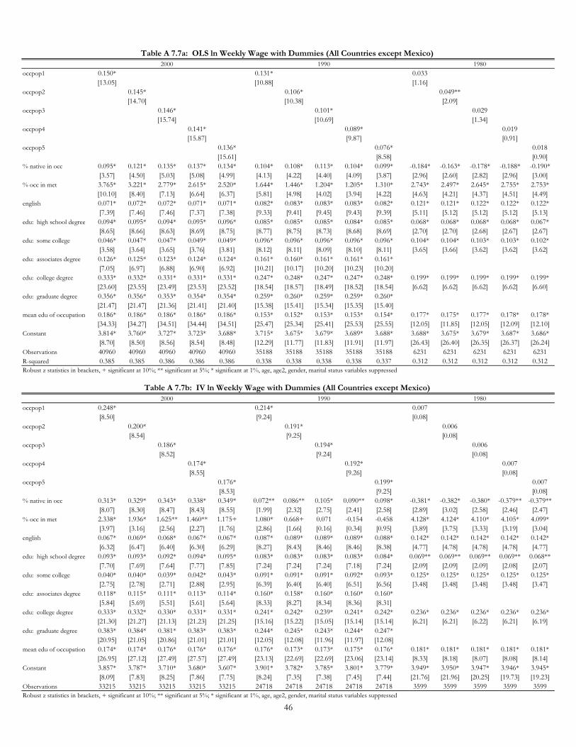
occpop1 0.150* 0.131* 0.033

[13.05] [10.88] [1.16]

occpop2 0.145* 0.106* 0.049**

[14.70] [10.38] [2.09]

occpop3 0.146* 0.101* 0.029

[15.74] [10.69] [1.34]

occpop4 0.141* 0.089* 0.019

[15.87] [9.87] [0.91]

occpop5 0.136* 0.076* 0.018

[15.61] [8.58] [0.90]

% native in occ 0.095* 0.121* 0.135* 0.137* 0.134* 0.104* 0.108* 0.113* 0.104* 0.099* -0.184* -0.163* -0.178* -0.188* -0.190*

[3.57] [4.50] [5.03] [5.08] [4.99] [4.13] [4.22] [4.40] [4.09] [3.87] [2.96] [2.60] [2.82] [2.96] [3.00]

% occ in met 3.765* 3.221* 2.779* 2.615* 2.520* 1.644* 1.446* 1.204* 1.205* 1.310* 2.743* 2.497* 2.645* 2.755* 2.753*

[10.10] [8.40] [7.13] [6.64] [6.37] [5.81] [4.98] [4.02] [3.94] [4.22] [4.63] [4.21] [4.37] [4.51] [4.49]

english 0.071* 0.072* 0.072* 0.071* 0.071* 0.082* 0.083* 0.083* 0.083* 0.082* 0.121* 0.121* 0.122* 0.122* 0.122*

[7.39] [7.46] [7.46] [7.37] [7.38] [9.33] [9.41] [9.45] [9.43] [9.39] [5.11] [5.12] [5.12] [5.12] [5.13]

edu: high school degree 0.094* 0.095* 0.094* 0.095* 0.096* 0.085* 0.085* 0.085* 0.084* 0.085* 0.068* 0.068* 0.068* 0.068* 0.067*

[8.65] [8.66] [8.63] [8.69] [8.75] [8.77] [8.75] [8.73] [8.68] [8.69] [2.70] [2.70] [2.68] [2.67] [2.67]

edu: some college 0.046* 0.047* 0.047* 0.049* 0.049* 0.096* 0.096* 0.096* 0.096* 0.096* 0.104* 0.104* 0.103* 0.103* 0.102*

[3.58] [3.64] [3.65] [3.76] [3.81] [8.12] [8.11] [8.09] [8.10] [8.11] [3.65] [3.66] [3.62] [3.62] [3.62]

edu: associates degree 0.126* 0.125* 0.123* 0.124* 0.124* 0.161* 0.160* 0.161* 0.161* 0.161*

[7.05] [6.97] [6.88] [6.90] [6.92] [10.21] [10.17] [10.20] [10.23] [10.20]

edu: college degree 0.333* 0.332* 0.331* 0.331* 0.331* 0.247* 0.248* 0.247* 0.247* 0.248* 0.199* 0.199* 0.199* 0.199* 0.199*

[23.60] [23.55] [23.49] [23.53] [23.52] [18.54] [18.57] [18.49] [18.52] [18.54] [6.62] [6.62] [6.62] [6.62] [6.60]

edu: graduate degree 0.356* 0.356* 0.353* 0.354* 0.354* 0.259* 0.260* 0.259* 0.259* 0.260*

[21.47] [21.47] [21.36] [21.41] [21.40] [15.38] [15.41] [15.34] [15.35] [15.40]

mean edu of occupation 0.186* 0.186* 0.186* 0.186* 0.186* 0.153* 0.152* 0.153* 0.153* 0.154* 0.177* 0.175* 0.177* 0.178* 0.178*

[34.33] [34.27] [34.51] [34.44] [34.51] [25.47] [25.34] [25.41] [25.53] [25.55] [12.05] [11.85] [12.05] [12.09] [12.10]

Constant 3.814* 3.760* 3.727* 3.723* 3.688* 3.715* 3.675* 3.679* 3.689* 3.688* 3.688* 3.675* 3.679* 3.687* 3.686*

[8.70] [8.50] [8.56] [8.54] [8.48] [12.29] [11.77] [11.83] [11.91] [11.97] [26.43] [26.40] [26.35] [26.37] [26.24]

Observations 40960 40960 40960 40960 40960 35188 35188 35188 35188 35188 6231 6231 6231 6231 6231

R-squared 0.385 0.385 0.386 0.386 0.386 0.338 0.338 0.338 0.338 0.337 0.312 0.312 0.312 0.312 0.312

occpop1 0.248* 0.214* 0.007

[8.50] [9.24] [0.08]

occpop2 0.200* 0.191* 0.006

[8.54] [9.25] [0.08]

occpop3 0.186* 0.194* 0.006

[8.52] [9.24] [0.08]

occpop4 0.174* 0.192* 0.007

[8.55] [9.26] [0.08]

occpop5 0.176* 0.199* 0.007

[8.53] [9.25] [0.08]

% native in occ 0.313* 0.329* 0.343* 0.338* 0.349* 0.072** 0.086** 0.105* 0.090** 0.098* -0.381* -0.382* -0.380* -0.379** -0.379**

[8.07] [8.30] [8.47] [8.43] [8.55] [1.99] [2.32] [2.75] [2.41] [2.58] [2.89] [3.02] [2.58] [2.46] [2.47]

% occ in met 2.338* 1.936* 1.625** 1.460** 1.175+ 1.080* 0.668+ 0.071 -0.154 -0.458 4.128* 4.124* 4.110* 4.105* 4.099*

[3.97] [3.16] [2.56] [2.27] [1.76] [2.86] [1.66] [0.16] [0.34] [0.95] [3.89] [3.75] [3.33] [3.19] [3.04]

english 0.067* 0.069* 0.068* 0.067* 0.067* 0.087* 0.089* 0.089* 0.089* 0.088* 0.142* 0.142* 0.142* 0.142* 0.142*

[6.32] [6.47] [6.40] [6.30] [6.29] [8.27] [8.43] [8.46] [8.46] [8.38] [4.77] [4.78] [4.78] [4.78] [4.77]

edu: high school degree 0.093* 0.093* 0.092* 0.094* 0.095* 0.083* 0.083* 0.083* 0.083* 0.084* 0.069** 0.069** 0.069** 0.069** 0.068**

[7.70] [7.69] [7.64] [7.77] [7.85] [7.24] [7.24] [7.24] [7.18] [7.24] [2.09] [2.09] [2.09] [2.08] [2.07]

edu: some college 0.040* 0.040* 0.039* 0.042* 0.043* 0.091* 0.091* 0.091* 0.092* 0.093* 0.125* 0.125* 0.125* 0.125* 0.125*

[2.75] [2.78] [2.71] [2.88] [2.95] [6.39] [6.40] [6.40] [6.51] [6.56] [3.48] [3.48] [3.48] [3.48] [3.47]

edu: associates degree 0.118* 0.115* 0.111* 0.113* 0.114* 0.160* 0.158* 0.160* 0.160* 0.160*

[5.84] [5.69] [5.51] [5.61] [5.64] [8.33] [8.27] [8.34] [8.36] [8.31]

edu: college degree 0.333* 0.332* 0.330* 0.331* 0.331* 0.241* 0.242* 0.239* 0.241* 0.242* 0.236* 0.236* 0.236* 0.236* 0.236*

[21.30] [21.27] [21.13] [21.23] [21.25] [15.16] [15.22] [15.05] [15.14] [15.14] [6.21] [6.21] [6.22] [6.21] [6.19]

edu: graduate degree 0.383* 0.384* 0.381* 0.383* 0.383* 0.244* 0.245* 0.243* 0.244* 0.247*

[20.95] [21.05] [20.86] [21.01] [21.01] [12.05] [12.08] [11.96] [11.97] [12.08]

mean edu of occupation 0.174* 0.174* 0.176* 0.176* 0.176* 0.176* 0.173* 0.173* 0.175* 0.176* 0.181* 0.181* 0.181* 0.181* 0.181*

[26.95] [27.12] [27.49] [27.57] [27.49] [23.13] [22.69] [22.69] [23.06] [23.14] [8.33] [8.18] [8.07] [8.08] [8.14]

Constant 3.857* 3.787* 3.710* 3.680* 3.607* 3.901* 3.782* 3.785* 3.801* 3.779* 3.949* 3.950* 3.947* 3.946* 3.945*

[8.09] [7.83] [8.25] [7.86] [7.75] [8.24] [7.35] [7.38] [7.45] [7.44] [21.76] [21.96] [20.25] [19.73] [19.23]

Observations 33215 33215 33215 33215 33215 24718 24718 24718 24718 24718 3599 3599 3599 3599 3599

Robust z statistics in brackets, + significant at 10%; ** significant at 5%; * significant at 1%, age, age2, gender, marital status variables suppressed

Robust z statistics in brackets, + significant at 10%; ** significant at 5%; * significant at 1%, age, age2, gender, marital status variables suppressed

Table A 7.7b: IV ln Weekly Wage with Dummies (All Countries except Mexico)

2000 1990 1980

Table A 7.7a: OLS ln Weekly Wage with Dummies (All Countries except Mexico)

2000 1990 1980

46

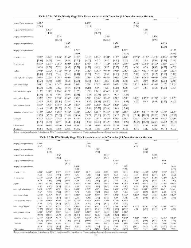
occpop1*cntrymn in occ 1.240* 1.249* 0.162

[12.68] [11.18] [0.74]

occpop2*cntrymn in occ 1.393* 1.274* 0.256

[14.30] [11.85] [1.21]

occpop3*cntrymn in occ 1.578* 1.356* 0.196

[15.78] [12.53] [0.91]

occpop4*cntrymn in occ 1.687* 1.374* 0.138

[16.47] [12.60] [0.63]

occpop5*cntrymn in occ 1.769* 1.377* 0.132

[16.90] [12.41] [0.58]

% native in occ 0.096* 0.124* 0.148* 0.161* 0.170* 0.103* 0.115* 0.124* 0.125* 0.128* -0.193* -0.180* -0.186* -0.193* -0.194*

[3.58] [4.60] [5.44] [5.89] [6.20] [4.07] [4.51] [4.87] [4.90] [5.00] [3.10] [2.85] [2.90] [2.98] [2.98]

% occ in met 3.813* 3.271* 2.784* 2.504* 2.279* 1.745* 1.441* 1.164* 1.055* 0.989* 2.846* 2.708* 2.755* 2.826* 2.831*

[10.20] [8.51] [7.12] [6.33] [5.71] [6.22] [5.03] [3.97] [3.55] [3.29] [4.84] [4.53] [4.52] [4.57] [4.53]

english 0.071* 0.072* 0.072* 0.071* 0.071* 0.082* 0.083* 0.083* 0.083* 0.083* 0.121* 0.121* 0.121* 0.121* 0.121*

[7.39] [7.43] [7.44] [7.41] [7.41] [9.38] [9.47] [9.50] [9.50] [9.49] [5.11] [5.12] [5.12] [5.12] [5.12]

edu: high school degree 0.094* 0.094* 0.094* 0.094* 0.095* 0.086* 0.086* 0.086* 0.086* 0.086* 0.068* 0.068* 0.068* 0.068* 0.068*

[8.60] [8.60] [8.60] [8.63] [8.66] [8.80] [8.84] [8.85] [8.84] [8.86] [2.69] [2.69] [2.69] [2.68] [2.68]

edu: some college 0.046* 0.046* 0.047* 0.048* 0.048* 0.096* 0.097* 0.097* 0.097* 0.098* 0.103* 0.104* 0.103* 0.103* 0.103*

[3.53] [3.58] [3.62] [3.69] [3.73] [8.15] [8.19] [8.21] [8.23] [8.26] [3.64] [3.65] [3.64] [3.63] [3.63]

edu: associates degree 0.126* 0.125* 0.124* 0.125* 0.125* 0.161* 0.161* 0.161* 0.162* 0.162*

[7.03] [6.99] [6.96] [6.97] [6.98] [10.23] [10.21] [10.24] [10.25] [10.24]

edu: college degree 0.332* 0.331* 0.330* 0.330* 0.330* 0.248* 0.248* 0.248* 0.248* 0.248* 0.199* 0.199* 0.199* 0.199* 0.199*

[23.55] [23.50] [23.44] [23.44] [23.43] [18.57] [18.61] [18.57] [18.58] [18.58] [6.63] [6.63] [6.63] [6.62] [6.62]

edu: graduate degree 0.356* 0.355* 0.354* 0.354* 0.353* 0.261* 0.262* 0.261* 0.261* 0.262*

[21.46] [21.45] [21.37] [21.38] [21.36] [15.51] [15.52] [15.48] [15.49] [15.51]

mean edu of occupation 0.185* 0.183* 0.183* 0.182* 0.181* 0.152* 0.151* 0.151* 0.151* 0.151* 0.178* 0.177* 0.178* 0.178* 0.178*

[33.98] [33.75] [33.66] [33.48] [33.36] [25.28] [25.10] [25.07] [25.12] [25.10] [12.14] [12.01] [12.07] [12.08] [12.07]

Constant 3.810* 3.773* 3.743* 3.729* 3.705* 3.725* 3.694* 3.689* 3.689* 3.682* 3.692* 3.683* 3.685* 3.690* 3.690*

[8.70] [8.57] [8.57] [8.54] [8.49] [12.31] [12.00] [11.99] [12.00] [11.99] [26.37] [26.31] [26.23] [26.22] [26.16]

Observations 40960 40960 40960 40960 40960 35188 35188 35188 35188 35188 6231 6231 6231 6231 6231

R-squared 0.384 0.385 0.386 0.386 0.386 0.338 0.338 0.339 0.339 0.339 0.312 0.312 0.312 0.312 0.312

occpop1*cntrymn in occ 1.936* 1.714* 0.048

[8.47] [9.28] [0.08]

occpop2*cntrymn in occ 1.701* 1.611* 0.045

[8.53] [9.31] [0.08]

occpop3*cntrymn in occ 1.642* 1.618* 0.045

[8.53] [9.31] [0.08]

occpop4*cntrymn in occ 1.596* 1.602* 0.046

[8.55] [9.32] [0.08]

occpop5*cntrymn in occ 1.598* 1.617* 0.046

[8.55] [9.32] [0.08]

% native in occ 0.284* 0.294* 0.301* 0.300* 0.303* 0.047 0.054 0.061+ 0.055 0.056 -0.382* -0.382* -0.382* -0.381* -0.381*

[7.63] [7.80] [7.91] [7.90] [7.95] [1.32] [1.52] [1.69] [1.54] [1.58] [3.06] [3.11] [2.94] [2.91] [2.92]

% occ in met 3.160* 2.872* 2.738* 2.664* 2.579* 1.532* 1.293* 1.061* 1.000* 0.931** 4.136* 4.134* 4.129* 4.129* 4.127*

[5.79] [5.14] [4.85] [4.69] [4.50] [4.30] [3.53] [2.81] [2.62] [2.42] [4.18] [4.08] [3.93] [3.91] [3.87]

english 0.067* 0.068* 0.068* 0.067* 0.067* 0.088* 0.089* 0.089* 0.089* 0.089* 0.142* 0.142* 0.142* 0.142* 0.142*

[6.32] [6.40] [6.38] [6.35] [6.35] [8.36] [8.46] [8.47] [8.48] [8.46] [4.78] [4.78] [4.78] [4.78] [4.78]

edu: high school degree 0.093* 0.093* 0.092* 0.093* 0.093* 0.083* 0.083* 0.084* 0.083* 0.084* 0.069** 0.069** 0.069** 0.069** 0.069**

[7.67] [7.68] [7.66] [7.71] [7.74] [7.25] [7.27] [7.28] [7.27] [7.29] [2.09] [2.09] [2.09] [2.09] [2.08]

edu: some college 0.040* 0.040* 0.040* 0.041* 0.041* 0.091* 0.091* 0.091* 0.092* 0.092* 0.125* 0.125* 0.125* 0.125* 0.125*

[2.76] [2.76] [2.74] [2.81] [2.83] [6.41] [6.45] [6.45] [6.49] [6.51] [3.48] [3.48] [3.48] [3.48] [3.48]

edu: associates degree 0.118* 0.116* 0.115* 0.115* 0.116* 0.160* 0.160* 0.160* 0.160* 0.160*

[5.84] [5.76] [5.70] [5.74] [5.75] [8.37] [8.34] [8.37] [8.38] [8.36]

edu: college degree 0.332* 0.332* 0.331* 0.331* 0.331* 0.242* 0.243* 0.242* 0.243* 0.243* 0.236* 0.236* 0.236* 0.236* 0.236*

[21.27] [21.28] [21.20] [21.24] [21.26] [15.25] [15.31] [15.26] [15.29] [15.29] [6.21] [6.21] [6.22] [6.22] [6.21]

edu: graduate degree 0.383* 0.384* 0.383* 0.384* 0.384* 0.248* 0.249* 0.248* 0.248* 0.249*

[20.99] [21.06] [20.98] [21.04] [21.04] [12.25] [12.25] [12.21] [12.21] [12.25]

mean edu of occupation 0.173* 0.173* 0.174* 0.174* 0.174* 0.175* 0.174* 0.174* 0.174* 0.175* 0.181* 0.181* 0.181* 0.181* 0.181*

[26.70] [26.89] [27.10] [27.16] [27.13] [23.00] [22.77] [22.76] [22.92] [22.95] [8.66] [8.59] [8.58] [8.58] [8.61]

Constant 3.868* 3.831* 3.794* 3.777* 3.755* 3.935* 3.881* 3.882* 3.888* 3.883* 3.949* 3.949* 3.948* 3.948* 3.948*

[8.16] [8.02] [8.22] [8.05] [8.02] [8.29] [7.90] [7.92] [7.95] [7.95] [21.71] [21.76] [21.13] [21.03] [20.94]

Observations 33215 33215 33215 33215 33215 24718 24718 24718 24718 24718 3599 3599 3599 3599 3599

Robust z statistics in brackets, + significant at 10%; ** significant at 5%; * significant at 1%, age, age2, gender, marital status variables suppressed

Robust z statistics in brackets, + significant at 10%; ** significant at 5%; * significant at 1%, age, age2, gender, marital status variables suppressed

Table A 7.8b: IV ln Weekly Wage With Shares interacted with Dummies (All Countries except Mexico)

2000 1990 1980

Table A 7.8a: OLS ln Weekly Wage With Shares interacted with Dummies (All Countries except Mexico)

2000 1990 1980

47