Imaging and fast features extraction of two-phase flows using ...
157
HAL Id: tel-03146817 https://tel.archives-ouvertes.fr/tel-03146817 Submitted on 19 Feb 2021 HAL is a multi-disciplinary open access archive for the deposit and dissemination of sci- entific research documents, whether they are pub- lished or not. The documents may come from teaching and research institutions in France or abroad, or from public or private research centers. L’archive ouverte pluridisciplinaire HAL, est destinée au dépôt et à la diffusion de documents scientifiques de niveau recherche, publiés ou non, émanant des établissements d’enseignement et de recherche français ou étrangers, des laboratoires publics ou privés. Imaging and fast features extraction of two-phase flows using electrical impedance tomography Chuihui Dang To cite this version: Chuihui Dang. Imaging and fast features extraction of two-phase flows using electrical impedance tomography. Physics [physics]. Ecole Centrale Marseille, 2020. English. NNT : 2020ECDM0006. tel-03146817
-
Upload
khangminh22 -
Category
Documents
-
view
0 -
download
0
Transcript of Imaging and fast features extraction of two-phase flows using ...

HAL Id: tel-03146817https://tel.archives-ouvertes.fr/tel-03146817
Submitted on 19 Feb 2021
HAL is a multi-disciplinary open accessarchive for the deposit and dissemination of sci-entific research documents, whether they are pub-lished or not. The documents may come fromteaching and research institutions in France orabroad, or from public or private research centers.
L’archive ouverte pluridisciplinaire HAL, estdestinée au dépôt et à la diffusion de documentsscientifiques de niveau recherche, publiés ou non,émanant des établissements d’enseignement et derecherche français ou étrangers, des laboratoirespublics ou privés.
Imaging and fast features extraction of two-phase flowsusing electrical impedance tomography
Chuihui Dang
To cite this version:Chuihui Dang. Imaging and fast features extraction of two-phase flows using electrical impedancetomography. Physics [physics]. Ecole Centrale Marseille, 2020. English. �NNT : 2020ECDM0006�.�tel-03146817�

École Doctorale : Physique et Sciences de la Matière (ED352)
Institut Fresnel & LTHC/CEA Cadarache
THÈSE DE DOCTORAT
pour obtenir le grade de
DOCTEUR de l’ÉCOLE CENTRALE de MARSEILLE
Discipline : Physique (Instrumentation)
IMAGING AND FAST FEATURES EXTRACTION OFTWO-PHASE FLOWS USING ELECTRICAL IMPEDANCE
TOMOGRAPHY
par
DANG Chunhui
Directeurs de thèse : BOURENNANE Salah, RICCIARDI Guillaume, BELLIS Cédric
Soutenue le 01 Octobre 2020
devant le jury composé de :
U. Hampel Professeur, Helmholtz-Zentrum Dresden-Rossendorf RapporteurN. Polydorides Professeur, University of Edinburgh RapporteurM. de Buhan Chargé de Recherche, CNRS - Université Paris Descartes ExaminatriceS. Mylvaganam Professeur, University College of Southeast Norway ExaminateurH-M. Prasser Professeur, ETH Zürich ExaminateurH. Schmidt Head of PKL and INKA, Framatome GmbH InvitéS. Bourennane Professeur, Ecole Centrale Marseille Directeur de thèseG. Ricciardi Expert senior, CEA Co-directeurC. Bellis Chargé de Recherche, LMA CNRS Encadrant


iii
Declaration of Authorship
I, Chunhui DANG, declare that this thesis titled,“IMAGING AND FAST FEATURES EX-TRACTION OF TWO-PHASE FLOWS USING ELECTRICAL IMPEDANCE TOMOGRAPHY”and the work presented in it are my own. I confirm that:
• This work was done wholly or mainly while in candidature for a research degree atthis University.
• Where any part of this thesis has previously been submitted for a degree or any otherqualification at this University or any other institution, this has been clearly stated.
• Where I have consulted the published work of others, this is always clearly attributed.
• Where I have quoted from the work of others, the source is always given. With theexception of such quotations, this thesis is entirely my own work.
• I have acknowledged all main sources of help.
• Where the thesis is based on work done by myself jointly with others, I have madeclear exactly what was done by others and what I have contributed myself.
Signed:
Date:


v
“I know that new situations can be intimidating. You’re lookin’ around and it’s all scary anddifferent, but y’know. . . meeting them head-on, charging into ‘em like a bull - that’s how wegrow as people.”
Rick Sanchez
“The most precious things in one’s life are: curiosity about knowledge, pursuit of beauty,kindness to the world, and sympathy for others.”
My former teacher


vii
Abstract
With the advantages of non-intrusiveness, high acquisition rate and low-cost, ElectricalImpedance Tomography (EIT) has been successfully applied in several cases in multi-phase flow instrumentation and clinical imaging. Most EIT systems currently in use relyon a sequential excitation at neighboring electrodes with measurements at the remainingones, i.e. the adjacent strategy, while some alternative excitation strategies have provento be effective and easy to implement using modern hardwares. Amongst the so-calledfull-scan strategy shows certain advantages in terms of the robustness to measurementnoise and the quality of reconstructed image. The objective of this thesis is to assess theapplicability of an EIT system implementing full-scan strategy at a high acquisition ratein two-phase flow measurements. The first stage consists of evaluating the four excita-tion strategies, namely the adjacent, opposite, full-scan and trigonometric strategies, ona number of practical criteria and quality of the reconstructed images, and assessing theinfluences of electrode size on the performance of an EIT system. The results are worth-while to the design of practical EIT systems and the associated test sections. The secondstage develops a novel eigenvalue-based approach for phase fraction estimation leverag-ing the redundant measurements from full-scan strategy, the ill-posed EIT image recon-struction is circumvented. The third stage reviews and evaluates various image recon-struction methods for high contrast and fast evolving conductivity profiles, several feasi-ble reconstruction strategies, namely one-step 2.5D method, iterative 2D methods, andGREIT method, are selected to make benchmark reconstructions for a set of static exper-iments. Finally, the comprehensive EIT measurement mode comprised by the developedEIT system, the image reconstruction procedure and the proposed eigenvalue-based ap-proach, is applied to horizontal two-phase flow measurements under both laboratory andindustrial environments. The analysis of the measurement data provides insights on themerits and deficiencies of the measurement mode.
Key words: Electrical Impedance Tomography, full-scan strategy, two-phase flow, voidfraction, eigenvalues

viii
ix
Résumé
Avec les avantages de la non-intrusion, d’un taux d’acquisition èlevé et d’un faible coût, latomographie par impédance électrique (EIT) a été appliquée avec succès dans plusieurscas d’instrumentation de flux polyphasique et d’imagerie clinique. La plupart des sys-tèmes EIT actuellement utilisés reposent sur une excitation séquentielle aux électrodesvoisines avec des mesures sur les autres, c’est-à-dire la stratégie adjacente, tandis que cer-taines stratégies d’excitation alternatives se sont révélées efficaces et faciles à mettre enœuvre en utilisant des matériels modernes. Parmi elles, la stratégie <full-scan> présentecertains avantages en termes de robustesse au bruit de mesure et de qualité de l’imagereconstruite. L’objectif de cette thèse est d’évaluer l’applicabilité d’un système EIT met-tant en œuvre une stratégie de balayage complet à un taux d’acquisition élevé dans lesmesures de débit diphasiques. La première étape consiste à évaluer les quatre stratégiesd’excitation, à savoir les stratégies adjacentes, opposées, full-scan et trigonométriques,sur un certain nombre de critères pratiques et de qualité des images reconstruites, et àévaluer les influences de la taille des électrodes sur les performances d’un système EIT.Les résultats sont utiles à la conception de systèmes EIT et aux sections de test associées.La deuxième étape développe une nouvelle approche basée sur les valeurs propres pourl’estimation du taux de vide tirant parti des mesures redondantes de la stratégie de bal-ayage complet : la reconstruction d’image EIT mal conditionnée est ainsi contournée. Latroisième étape passe en revue et évalue diverses méthodes de reconstruction d’imagespour les profils de conductivité à contraste élevé et à évolution rapide. Plusieurs stratégiesde reconstruction réalisables, à savoir la méthode 2.5D en une itération, les méthodes 2Ditératives et la méthode GREIT, sont sélectionnées pour effectuer des reconstructions deréférence pour un ensemble d’expériences statiques. Enfin, le mode de mesure EIT com-plet, composé du système EIT développé, de la procédure de reconstruction d’image etde l’approche basée sur les valeurs propres, est appliqué aux mesures de débit en deuxphases horizontales en laboratoire et environnements industriels. L’analyse des donnéesdonne un aperçu des avantages et des inconvénients de ces méthodes de mesure.
Mots clés: Tomographie d’impédance électrique, la stratégie full-scan, valeurs propres,écoulement diphasique, taux de vide


xi
Acknowledgements
Foremost, I would like to express my sincere gratitude to my supervisor Guillaume Riccia-rdi for the continuous support of my Ph.D study and research, for his motivation, encour-agement, and immense knowledge. His guidance helped me in all the time of research andwriting of this thesis. I am also grateful to my co-supervisor Cédric Bellis for his valuablesupervision and inspiration, I learned a lot from him on rigorous thinking and scientificwriting. And I appreciate the help from my thesis director Salah Bourennane. I could nothave imagined having better supervisors and mentors for my Ph.D study.
Besides my superviosors, I would like to thank Schmidt Holger from Framatome GmbHand Saba Mylvaganam from USN, for their help in paper revisions and performing exper-iments that are essential to my Ph.D study. My sincere thanks also go to my colleaguesin LTHC of CEA Cadarache, for offering a professional and warmful environment for mystudy and work, their diverse exciting projects broadened my horizons. Amongst, I’d liketo give special thanks to my Ph.D-mate Mathieu Darnajou, for the stimulating discussionsas well as for the pleasing work trips, skiing, climbing, and music, oh, plus our first andprobably last international conference on EIT held in CHALET with Antoine Dupré.
I thank my fellow workmates in the lab: Naz Turankok, Lorenzo Longo, Roberto Capanna,Samy Mokhtari, Louise Bernadou, Benjamin Jourdy, for the countless delightful smalltalks, cafe breaks and lunches. Also I thank my colleagues in CEA Chinese Ph.D team:Jianwei Shi, Fang Chen, Hui Guo, Shengli Chen, Weifeng Zhou, Xiaoshu Ma, GuangzeYang, Shuo Li, Congjin Ding and others, and my friends in Aix en Provence: Siyun Wang,Chaowei Xu, for the afterwork activities, short hiking, and enjoyable chatting.
Last but not the least, I would like to thank my parents Dianjun Dang and Xiuli Zhi, my sis-ter Jiaojiao Dang and my girlfriend Xuan Guo, for supporting me spiritually and bringinghappiness to my daily life.


xiii
Contents
Abstract vii
List of Figures xv
List of Tables xix
List of Abbreviations xxi
List of Symbols xxiii
1 Context 1
2 Introduction 72.1 Flow imaging techniques . . . . . . . . . . . . . . . . . . . . . . . . . . . . . . 7
2.1.1 Radiation tomography . . . . . . . . . . . . . . . . . . . . . . . . . . . . 72.1.2 Ultrasonic tomography . . . . . . . . . . . . . . . . . . . . . . . . . . . 92.1.3 Electrical tomography . . . . . . . . . . . . . . . . . . . . . . . . . . . . 10
2.2 Electrical impedance tomography . . . . . . . . . . . . . . . . . . . . . . . . . 122.2.1 Forward model . . . . . . . . . . . . . . . . . . . . . . . . . . . . . . . . 122.2.2 Excitation strategy . . . . . . . . . . . . . . . . . . . . . . . . . . . . . . 162.2.3 3D effect . . . . . . . . . . . . . . . . . . . . . . . . . . . . . . . . . . . . 19
3 EIT system design for two-phase flow imaging 233.1 EIT systems developed in LTHC . . . . . . . . . . . . . . . . . . . . . . . . . . 23
3.1.1 ProME-T system . . . . . . . . . . . . . . . . . . . . . . . . . . . . . . . 243.1.2 ONE-SHOT system . . . . . . . . . . . . . . . . . . . . . . . . . . . . . . 26
3.2 Practical comparison of excitation strategies . . . . . . . . . . . . . . . . . . . 283.2.1 Representative frame rates . . . . . . . . . . . . . . . . . . . . . . . . . 293.2.2 Statistics of measurement amplitudes . . . . . . . . . . . . . . . . . . . 303.2.3 Sensitivity distributions . . . . . . . . . . . . . . . . . . . . . . . . . . . 313.2.4 Practical implementation criteria . . . . . . . . . . . . . . . . . . . . . 31
3.3 Influences of electrode size on EIT system performance . . . . . . . . . . . . 323.3.1 Total impedance spectrum . . . . . . . . . . . . . . . . . . . . . . . . . 333.3.2 Bulk impedance . . . . . . . . . . . . . . . . . . . . . . . . . . . . . . . . 343.3.3 Noise analysis . . . . . . . . . . . . . . . . . . . . . . . . . . . . . . . . . 353.3.4 Residual error analysis . . . . . . . . . . . . . . . . . . . . . . . . . . . . 37
3.4 Dual-plane test section design for the PKL facility . . . . . . . . . . . . . . . . 38
4 Eigenvalue-based approach using EIT raw data 434.1 Methodology . . . . . . . . . . . . . . . . . . . . . . . . . . . . . . . . . . . . . . 43
4.1.1 Mathematical basis . . . . . . . . . . . . . . . . . . . . . . . . . . . . . . 434.1.2 Impedance matrix and normalization . . . . . . . . . . . . . . . . . . . 44
4.2 Estimation of cross-sectional phase fraction . . . . . . . . . . . . . . . . . . . 464.2.1 Numerical simulations . . . . . . . . . . . . . . . . . . . . . . . . . . . . 46
xiv
4.2.2 Robustness of the proposed approach . . . . . . . . . . . . . . . . . . . 524.2.3 Validation by static experiments . . . . . . . . . . . . . . . . . . . . . . 54
5 Image reconstruction of highly contrasted profiles 575.1 Review of image reconstruction methods . . . . . . . . . . . . . . . . . . . . . 57
5.1.1 Back-projection . . . . . . . . . . . . . . . . . . . . . . . . . . . . . . . . 585.1.2 Least-squares methods . . . . . . . . . . . . . . . . . . . . . . . . . . . 585.1.3 Factorization method . . . . . . . . . . . . . . . . . . . . . . . . . . . . 635.1.4 Topological sensitivity . . . . . . . . . . . . . . . . . . . . . . . . . . . . 68
5.2 Imaging of two-phase flows . . . . . . . . . . . . . . . . . . . . . . . . . . . . . 715.2.1 2D or 3D reconstruction . . . . . . . . . . . . . . . . . . . . . . . . . . . 725.2.2 Benchmark reconstruction of static experiments . . . . . . . . . . . . 77
5.3 Quantitive comparisons of various excitation strategies . . . . . . . . . . . . 785.3.1 From synthetic data . . . . . . . . . . . . . . . . . . . . . . . . . . . . . 795.3.2 From experimental data . . . . . . . . . . . . . . . . . . . . . . . . . . . 85
6 Dynamic two-phase flow experiments 896.1 Horizontal two-phase flow regimes . . . . . . . . . . . . . . . . . . . . . . . . 896.2 Preliminary validation in LTHC . . . . . . . . . . . . . . . . . . . . . . . . . . . 916.3 Dynamic experiments in laboratory loop . . . . . . . . . . . . . . . . . . . . . 92
6.3.1 Experiment procedures . . . . . . . . . . . . . . . . . . . . . . . . . . . 936.3.2 Eigenvalue-based approach . . . . . . . . . . . . . . . . . . . . . . . . . 966.3.3 System calibration from NIM leading eigenvalue and AVF correlation 966.3.4 Temporal evolution of the leading eigenvalue . . . . . . . . . . . . . . 986.3.5 Stacked EIT tomogram . . . . . . . . . . . . . . . . . . . . . . . . . . . . 996.3.6 Tomogram binarization and flow visualization . . . . . . . . . . . . . 100
6.4 Dynamic experiments in industrial loop . . . . . . . . . . . . . . . . . . . . . 1026.4.1 Experiment procedures . . . . . . . . . . . . . . . . . . . . . . . . . . . 1026.4.2 Result analysis . . . . . . . . . . . . . . . . . . . . . . . . . . . . . . . . . 104
7 Conclusion 109
A Dual-plane test section design for PKL 113
B EIT and GRM tomograms for experiments in USN 117
Bibliography 121

xv
List of Figures
1.1 The main components of PKL facility, the developed EIT sensor would bemounted on one of the four hot legs. . . . . . . . . . . . . . . . . . . . . . . . . 2
2.1 Schematic of a fast X-ray scanner with three X-ray sources, adapted fromSalgado et al. (2010). Left: side view showing only one source with its twodetector arrays, right: top view showing three sources and their correspond-ing detectors. . . . . . . . . . . . . . . . . . . . . . . . . . . . . . . . . . . . . . 8
2.2 Schematic of the three ultrasonic sensing modes, using a 32 transducers sys-tem as example and a square-shaped object. . . . . . . . . . . . . . . . . . . . 9
2.3 A wire-mesh sensor with a 24£24 measurement grid, adapted from Nedeltchevet al. (2016). . . . . . . . . . . . . . . . . . . . . . . . . . . . . . . . . . . . . . . 10
2.4 The schematic of an ECT sensor, with 8 electrodes mounted on the insulatedpipe exterior. . . . . . . . . . . . . . . . . . . . . . . . . . . . . . . . . . . . . . . 11
2.5 Schematic of an EIT sensor with 16 electrodes (electrode index is given from1 to 16). The excitation currents are injected at electrodes (i , j ), differencevoltage is measured at neighboring electrodes. . . . . . . . . . . . . . . . . . 13
2.6 Schematics of the four excitation strategies, the blue dotted lines in (a) to (c)indicate the following electrode pairs for excitation. In (d) the trigonometricfunction with a frequency j = 4 is plotted, giving the excitation amplitude ateach electrode. . . . . . . . . . . . . . . . . . . . . . . . . . . . . . . . . . . . . 16
2.7 Schemes of EIT operating modes: (a) Current excitation at electrodes (i , j )with difference voltage measurements at neighboring electrodes; (b) Volt-age excitation at electrodes (i , j ) with difference voltage measurements atneighboring electrodes; (c) Voltage excitation at electrodes (i , j ) with volt-age measurement across R0 at each electrode. . . . . . . . . . . . . . . . . . . 18
2.8 An example finite element mesh for the case with Le = 1.2. . . . . . . . . . . 192.9 The current streamlines and equipotential lines in the domain with varying
electrode lengths Le = 0.02, 0.2, 0.7, 1.2. . . . . . . . . . . . . . . . . . . . . . . 202.10 Zoom-in plot of the current streamlines at the ends of the electrode for Le =
0.2. . . . . . . . . . . . . . . . . . . . . . . . . . . . . . . . . . . . . . . . . . . . 202.11 The current streamlines and equipotential lines in the domain for Le = 0.2
and Ld = 0.3, 0.7, the guarding electrodes are excited with the same voltagesas the main plane electrodes. . . . . . . . . . . . . . . . . . . . . . . . . . . . . 21
2.12 The current streamlines and equipotential lines in the domain for Le = 0.2and Ld = 0.3, 0.7, the guarding electrodes are grounded (at zero potential). . 21
3.1 Left: the ProME-T system in LTHC applying TDM with 16 electrodes. Right:the two sets of electrodes with different lengths available for ProME-T. . . . 24
3.2 Closed circuit between the source and drain electrodes for each excitationpattern. . . . . . . . . . . . . . . . . . . . . . . . . . . . . . . . . . . . . . . . . . 25
3.3 The ONE-SHOT system developed in LTHC using FDM with 16 electrodes,adapted from Darnajou et al. (2020). . . . . . . . . . . . . . . . . . . . . . . . . 27

xvi
3.4 Equivalent closed circuit of the ONE-SHOT EIT system. . . . . . . . . . . . . 273.5 2D forward simulation model with 16 evenly spaced electrodes. . . . . . . . 303.6 Locally averaged sensitivity distributions along one diameter for the excita-
tion strategies considered. . . . . . . . . . . . . . . . . . . . . . . . . . . . . . . 323.7 Practical implementation criteria, each normalized by the largest value among
the four excitation strategies. The value 1 is associated with the best practicalperformance and low values indicate relatively lower-performing strategies. 33
3.8 The module and phase of the total impedance changing with excitation fre-quencies, three different electrolyte conductivities are used for each elec-trode set. . . . . . . . . . . . . . . . . . . . . . . . . . . . . . . . . . . . . . . . . 34
3.9 Total and bulk impedances of each excitation pattern in the full-scan strat-egy, for two sets of electrodes. . . . . . . . . . . . . . . . . . . . . . . . . . . . . 35
3.10 Spectrums of the high and low amplitude measurements using ES2 elec-trodes, with homogeneous water of conductivity 750µS/cm in the test section. 36
3.11 The Signal to Noise Ratio (SNR) of two sets of electrodes. . . . . . . . . . . . 363.12 Relative errors of all measurements at 50kHz excitation frequency for ES1
and ES2. . . . . . . . . . . . . . . . . . . . . . . . . . . . . . . . . . . . . . . . . 373.13 Relative errors of the four types of measurements induced by multiplexing,
for both sets of electrodes. . . . . . . . . . . . . . . . . . . . . . . . . . . . . . . 393.14 Configuration of the working space for the dual-plane test section. . . . . . 403.15 From left to right: the real object, and the image reconstructions with ` =
16, 32, 64. . . . . . . . . . . . . . . . . . . . . . . . . . . . . . . . . . . . . . . . 41
4.1 Effect of the normalization on the entries of the impedance matrices in thecase of a single bubble. . . . . . . . . . . . . . . . . . . . . . . . . . . . . . . . . 45
4.2 Conductivity distribution patterns for the three canonical cases considered. 474.3 Entries of the normalized impedance matrix of the cases 2 and 3. . . . . . . 484.4 Eigenvalue array for some configurations corresponding to Case 1. . . . . . 484.5 Eigenvalue array of one bubble inclusion (r = 0.35) moving from d = 0 to
d = 0.6. . . . . . . . . . . . . . . . . . . . . . . . . . . . . . . . . . . . . . . . . . 494.6 Map of the logarithm of the sensitivity distribution, left: source/drain at
electrodes (1,7) and measurement at electrodes (12,13), refer to Figure 2.5for electrode numbering; right: full-scan strategy. . . . . . . . . . . . . . . . . 49
4.7 Eigenvalues vs. void fraction for Case 1. . . . . . . . . . . . . . . . . . . . . . . 504.8 Eigenvalue arrays and ∏(16) as a function of h for Case 2. . . . . . . . . . . . . 514.9 Eigenvalues vs. void fraction for Case 3. . . . . . . . . . . . . . . . . . . . . . . 514.10 Eigenvalue trends obtained with noisy data in Case 1. . . . . . . . . . . . . . 524.11 ∏(16) and
P15|∏| vs. ¥ for various values of R in Case 1. . . . . . . . . . . . . . . 53
4.12 ∏(16) vs. h in Case 2. . . . . . . . . . . . . . . . . . . . . . . . . . . . . . . . . . . 534.13 3D simulation model to compare with the static experiments, non-conductive
rods with the same height of the model would be used to emulate the bubbleinclusion. . . . . . . . . . . . . . . . . . . . . . . . . . . . . . . . . . . . . . . . . 55
4.14 Comparison between 3D simulations and experimental static experimentsfor the cases 1 and 3: eigenvalue ∏(16) as a function of the void fraction ¥. . . 55
4.15 Comparison between 3D simulations and experimental static experimentsfor Case 2. . . . . . . . . . . . . . . . . . . . . . . . . . . . . . . . . . . . . . . . 56
5.1 Schematic of the factorization method with four electrodes on the boundary.The test function gives significant value for a test point z inside the object≠i . 63
5.2 Schematics of the real conductivity profiles with one and three objects in-side the domain. . . . . . . . . . . . . . . . . . . . . . . . . . . . . . . . . . . . 66

xvii
5.3 log∏k and loghtz , vki2 changing with k for one and three objects cases. Oneout of two points are plotted for the sake of clarity. . . . . . . . . . . . . . . . 66
5.4 Image reconstructions using the FM for one and three objects cases. . . . . 675.5 Reconstructions using the MUSIC algorithm for one and three objects cases. 685.6 log∏k and loghtz , vki2 associated with noisy data for one and three objects
cases. One out of two points are plotted for the sake of clarity. . . . . . . . . 685.7 Reconstructions from the FM and MUSIC methods with noisy data for one
and three objects cases. . . . . . . . . . . . . . . . . . . . . . . . . . . . . . . . 695.8 Schematic of measurment, reference and adjoint configurations simulated,
Eexc represents the excitation electrode. . . . . . . . . . . . . . . . . . . . . . 705.9 The image case studied and the resulting adjoint sensitivity map using four
electrodes. . . . . . . . . . . . . . . . . . . . . . . . . . . . . . . . . . . . . . . . 715.10 The 3D forward model with a ball-shaped object locating at the middle of
electrode plane. . . . . . . . . . . . . . . . . . . . . . . . . . . . . . . . . . . . . 735.11 The 3D image reconstruction for the case with a ball located at electrode
plane. . . . . . . . . . . . . . . . . . . . . . . . . . . . . . . . . . . . . . . . . . . 735.12 The 3D fine inverse model used for 2.5D reconstruction and the final recon-
structed image. . . . . . . . . . . . . . . . . . . . . . . . . . . . . . . . . . . . . 745.13 2D inverse model with coarse mesh used for image reconstruction. . . . . . 755.14 2D reconstructions using iterative Tikhonov and TV regularized methods
and 3D measurement data. . . . . . . . . . . . . . . . . . . . . . . . . . . . . . 755.15 2D reconstructions using iterative Tikhonov and TV regularized methods
and 2D measurement data. . . . . . . . . . . . . . . . . . . . . . . . . . . . . . 765.16 2D GREIT reconstructions using the best inverse matrix R estimated from
nt = 1000 and nt = 3000 small targets. . . . . . . . . . . . . . . . . . . . . . . . 775.17 Image reconstructions using selected methods for static experiments with
ES1 electrodes, center rod case. . . . . . . . . . . . . . . . . . . . . . . . . . . . 775.18 Image reconstructions using selected methods for static experiments with
ES1 electrodes, boundary rod case. . . . . . . . . . . . . . . . . . . . . . . . . . 785.19 Image reconstructions using selected methods for static experiments with
ES1 electrodes, two rods case. . . . . . . . . . . . . . . . . . . . . . . . . . . . . 785.20 Image reconstructions using selected methods for static experiments with
ES2 electrodes, center rod case. . . . . . . . . . . . . . . . . . . . . . . . . . . . 785.21 Image reconstructions using selected methods for static experiments with
ES2 electrodes, boundary rod case. . . . . . . . . . . . . . . . . . . . . . . . . . 795.22 The L-curve for full-scan strategy with NOSER method. The point at maxi-
mum curvature corresponds to the optimal hyperparameter. . . . . . . . . . 805.23 [Case 1] Profiles of the reconstructed conductivity contrasts ¢æh
id along onediameter for the different excitation strategies and reconstruction methodsconsidered. . . . . . . . . . . . . . . . . . . . . . . . . . . . . . . . . . . . . . . 82
5.24 [Case 4] Profiles of the reconstructed conductivity contrasts ¢æhid along one
diameter for the different excitation strategies and reconstruction methodsconsidered. . . . . . . . . . . . . . . . . . . . . . . . . . . . . . . . . . . . . . . . 82
5.25 Logarithm of the global identification errors ≤id, normalized by the largesterror among the four excitation strategies for each case and each reconstruc-tion method. The value 0 is associated with the lowest-performing strategyand low values indicate relatively better performances. . . . . . . . . . . . . . 83
5.26 Logarithm of the geometrical area errors ≤A, normalized by the largest erroramong the four excitation strategies for each case and each reconstructionmethod. The value 0 is associated with the lowest-performing strategy andlow values indicate relatively better performances. . . . . . . . . . . . . . . . 84

xviii
5.27 Logarithm of the positioning errors ≤p, normalized by the largest error amongthe four excitation strategies for each case and each reconstruction method.The value 0 is associated with the lowest-performing strategy and low valuesindicate relatively better performances. . . . . . . . . . . . . . . . . . . . . . . 85
6.1 Sketches of various horizontal gas-water flow regimes. . . . . . . . . . . . . . 906.2 Flow regime map of the horizontal air-water flow in a pipe with 50 mm di-
ameter, adapted from Mandhane et al. (1974). Hatched regions are regimeboundaries by observation. . . . . . . . . . . . . . . . . . . . . . . . . . . . . . 91
6.3 The EIT tomogram with ES1 electrodes comparing to a frame taken from thehigh speed video. . . . . . . . . . . . . . . . . . . . . . . . . . . . . . . . . . . . 92
6.4 The EIT tomogram with ES2 electrodes comparing to a frame taken from thehigh speed video. . . . . . . . . . . . . . . . . . . . . . . . . . . . . . . . . . . . 93
6.8 System calibration diagram: eigenvalue ∏maxmean vs. reference AVF from GRM,
with indication of the flow regimes. Stars indicate the experiments selectedin Fig. 6.9. . . . . . . . . . . . . . . . . . . . . . . . . . . . . . . . . . . . . . . . 97
6.9 Temporal evolution of the leading eigenvalue∏max of Z f along time (or framef ) for the five selected experiments identified in Fig. 6.7 and 6.8. The cross-sectional images at time t = 5.3 s (vertical dashed line) are shown in Fig. 6.10. 98
6.10 Cross-sectional image reconstructions ¢æ= (æ°æref) for the selected casesand at the time t = 5.3s, indicated by the black dashed lines in Fig. 6.9. . . . 99
6.11 (top) Raw EIT tomograms, i.e. ¢æ, (middle) binarized EIT tomograms, and(bottom) reference GRM tomograms, for the experimental sets consideredof slug, stratified wavy and annular flows. The abscissae represents the mea-surement time in second (or frame f ). The vertical dashed lines correspondsto t = 5.3 s with the corresponding cross-sectional images shown in the rightpanels. . . . . . . . . . . . . . . . . . . . . . . . . . . . . . . . . . . . . . . . . . 101
6.12 Schematic of the BENSON loop. The dual-plane EIT test section was in-stalled in the horizontal test pipe. . . . . . . . . . . . . . . . . . . . . . . . . . 103
6.13 Dual-plane EIT system used for the BENSON experiments. . . . . . . . . . . 1036.14 Correlation between the void fraction and the steam quality at different wa-
ter mass flow rates. . . . . . . . . . . . . . . . . . . . . . . . . . . . . . . . . . . 1046.15 Spectrum analysis of the high and low amplitude measurements during the
BENSON experiments. . . . . . . . . . . . . . . . . . . . . . . . . . . . . . . . . 1056.16 The Signal to Noise Ratio (SNR) of the system in the BENSON loop compar-
ing to that in laboratory environment. . . . . . . . . . . . . . . . . . . . . . . . 1056.17 Relative errors of repeating measurements at 50 kHz excitation frequency for
the BENSON and ES2 in LTHC. . . . . . . . . . . . . . . . . . . . . . . . . . . . 1066.18 Identifying the water level from the indices of the normalized impedance
matrix, void fraction ¥= 0.52. . . . . . . . . . . . . . . . . . . . . . . . . . . . . 107
A.1 Schematic of the EIT test section design for PKL facility. . . . . . . . . . . . . 114A.2 Schematic of the electrodes used in the EIT test section for PKL facility. . . . 115

xix
List of Tables
2.1 Number N im of independent measurements and redundancy ratio relatively
to the number Nm of measurements for the various strategies, consideringan EIT system with 16 electrodes. . . . . . . . . . . . . . . . . . . . . . . . . . 18
3.1 Estimated acquisition frame rates (fps) for the excitation strategies consid-ered and using EIT systems with 16 electrodes. . . . . . . . . . . . . . . . . . 29
3.2 Mean and standard deviation of the boundary measurements for the variousexcitation strategies and a 16 electrodes EIT system. . . . . . . . . . . . . . . 30
3.3 Mean and standard deviation of the sensitivity distributions for the variousexcitation strategies and a 16 electrodes EIT system, see also Figure 3.6(a). . 32
5.1 Geometric parameters defining the cases considered with the circular ob-ject(s) to be reconstructed. . . . . . . . . . . . . . . . . . . . . . . . . . . . . . 80
5.2 Reconstructions ¢æhid of the conductivity contrast from synthetic measure-
ments and using the NOSER method and TV regularization. . . . . . . . . . . 815.3 Reconstructions of the conductivity contrast ¢æh
id from experimental dataand using the NOSER method or TV regularization. . . . . . . . . . . . . . . . 87
6.1 Test matrix of the experiments in the BENSON loop. . . . . . . . . . . . . . . 1046.2 Mean relative error RE for various EIT configurations. . . . . . . . . . . . . . 106


xxi
List of Abbreviations
AI Analogue InputAO Analogue OutputAT3NA Algorithme de Tomographie en 3D NOSER et Aplanissement (French)BNC Bayonet Neill-Concelman connectorCEA French Alternative Energies and Atomic Energy CommissionCT Computed TomographyDIM Differential Impedance MatrixDO Digital OutputDtN Dirichlet-to-NeumannECT Electrical Capacitance Tomography
EIDORSElectrical Impedance Tomography and Diffuse Optical Tomography ReconstructionSoftware
EIT Electrical Impedance TomographyES1 Electrode Set 1ES2 Electrode Set 2FBP Filtered Back-ProjectionFDM Frequency Division MultiplexingFEM Finite Element MethodFFT Fast Fourier TransformFPGA Field Programmable Gate Arrayfps frames per secondGREIT Graz consensus Reconstruction algorithm for EITGRM Gamma-Ray Meter
LTHCLaboratory of analytical Thermo-hydraulics and Hydromechanics of Core andCircuits
MAP Maximum A PosterioriMUSIC MUltiple-SIgnal-ClassificationNIM Normalized Impedance MatrixNOSER Newton’s one-step error reconstructionNtD Neumann-to-DirichletONE-SHOT ONe Excitation for Simultaneous High-speed Operation Tomography (French)PCB Printed Circuit BoardPDIPM Primal Dual-Interior Point MethodsPKL PWR Integral System Test FacilityPMMA PolymethylmethacrylateProME-T Prototype pour Mesures Electriques par TomographiePWR Pressurized Water ReactorRE Relative ErrorSNR Signal to Noise RatioTDM Time Division MultiplexingTV Total VariationUSN University College of Southeast Norway


xxiii
List of Symbols
A area of water segmentAid area of the object(s) in the segmented reconstructionAtrue area of the object(s) in the true imageA a matrix representation of the Galerkin projectionCe double layer capacitanced distance of the single bubble to the domain centerdid distance of the the objects barycenter to the origin in the reconstructed imagedtrue distance of the the objects barycenter to the origin in the true imageD internal diameter of the test sectionDz (x) dipole functiond an arbitrary unit vectorf boundary current densityfexc frequency of the excitation signalf an orthogonal basis formed by fi
fi i -th boundary excitations of trigonometric strategyG(x, s) Green’s function in 2
G≠(·, z) Green’s function in the domain≠h height of the bubble segmenthw height of the water segmentI0 a fixed amplitudeIe a given current excitationIk, j boundary excitation at electrode k in j -th excitation pattern of trigonometric strategyIZ current passing through the system in an excitation patternI identity matrixJ2(æ";a) topological derivative associated with æ";a
J (æ) an objective function for EIT problemJ ("; a) an objective function associated with≠"(a)J Jacobian matrix` number of electrodesLd distance between the guarding and main electrode planesLdi s distance between the dual planesLe length of the electrodesLE I T total length of the dual-plane test sectionLi so distance between the electrodes and the grounded pipe`max theoretical limit to ` for a finite accuracy acquisition systemL regularization matrixm0 the number of eigenvalues and eigenvectors considered in factorization methodm water mass flow raten0 index corresponding to the minimum eigenvalue over the noise levelnbub number of uniformly distributed bubblesnc number of repeating framesne index of the element in the finite element model

xxiv
Nd number of sampling points for one frame of ONE-SHOTNe number of excitation patternsNel number of elements in the finite element modelNm number of measurementsN i
m number of independent measurementsNp number of periods per excitation patternNsp number of samples per periodn unit outward normal vector on the boundaryp exponent coefficient of generalized Tikhonov regularizationP (x|b) conditional probability of x given bP an orthonormal projector onto the basis fQ(æ) regularization termr radius of a single bubbler0 radius of the simulation geometryrdi s radius of uniformly distributed bubblesre equivalent radius of the uniformly distributed bubblesR0 constant resistorRe charge transfer resistanceR contrast between the high and low conductivityR f rank of a matrix or operatorR inverse matrix
2 infinite two-dimensional real coordinate space`¶ `-dimensional vector space
s(i ,k) j sensitivity of Vi k to a local conductivity perturbation in j -th elementS j overall sensitivity in the j -th elementtz trace of Tz
t f r ame acquisition time for one frameTz test function for factorization methodu electrical fieldu0 electrical field of reference caseuad j adjoint electrical fieldur e f reference electrical fieldui voltage field associated with i -th current patternuk voltage field computed using the k-th voltage measurement as an excitation currentu|@≠ boundary potential of image caseu0|@≠ boundary potential of reference caseU (æ) a set of simulated boundary measurements associated with ævi deal ideal velocity estimationvr eal real velocity estimationvz a harmonic function of Dz
v (i ) i -th eigenvector of the impedance matrixV0 amplitude of the excitation voltageVR voltage measurement across R0
Vi k a measurement at electrode pair k with excitation at electrode pair iVi , j voltage difference between source i and drain jV a set of boundary measurementsVh reference measurements with homogeneous profileVi image measurements with extra object(s) insidexFFT
i discrete amplitude at frequency i after FFTZ sour ce contact impedance at the source electrodeZ dr ai n contact impedance at the drain electrode

xxv
Z tot total impedanceZi , j bulk impedance between source i and drain jZi , j normalized bulk impedance between source i and drain jZ impedance matrixZ 0 impedance matrix of reference case¢Z difference impedance matrix between Z and Z 0
Z normalized impedance matrixZm impedance matrix of m-th frameZmean mean impedance matrix of consecutive frames
Æ hyper-parameter∞ electric admittivity± Dirac’s delta function±d distinguishability≤ electric permittivity≤id global identification error≤A geometrical area error≤p positioning error"0ri radius of≠i assumed in MUSIC method¥ void fraction¥l liquid volume fractionµz the angle between tz and R(§æ°§0)1/2
∑ condition number of a matrix∏(16)
noi s y leading eigenvalue of the noisy data
∏(i ) i -th eigenvalue of the impedance matrix∏(`) leading eigenvalueP15
|∏| sum of the absolute value of the first 15 eigenvalues
∏(16)mean leading eigenvalue of Zmean
§0 NtD map of reference case§æ NtD map of image caseª relative error of the eigenvalues¶ relative NtD mapæ electric conductivityæ j local conductivity in the j -th element±æ j a conductivity perturbation to æ j
æid approximated conductivity profile that minimizes the cost functionæid segmented profile of æid
æk conductivity estimation at step kæk+1 conductivity estimation at step k+1±æk update of conductivity approximation at step kæref reference conductivity profileætrue true conductivity profileæ";a conductivity profile with the object≠"(a)& relative error of the estimated velocityøi deal ideal time delay between the two electrode planesør eal real time delay between the two electrode planes©(æ) cost function used in the least squares methods©00 Hessian matrix¬ steam quality! excitation frequency

xxvi
! j angular frequency of trigonometric excitation≠ a two- or three-dimensional domain@≠ boundary of the domain≠≠"(a) a small object with a characteristic radius " at location a≠i a set of non-conductive inclusions@≠i boundary of the inclusions≠i

xxvii
Dedicated to my beloved family, fortheir endless love, support andinspiration during my Ph.D. . .


1
Chapter 1
Context
Tomography means imaging sections or by sectioning, through exerting penetrating wavesand receiving resulting waves. Usually images are obtained through tomographic recon-structions, such as the X-ray computed tomography. The principle has been applied tomany research fields: geophysics, material science, plasma physics, archaeology, to citebut a few. Different types of penetrating waves have been used, including radiation beams(X-ray, g-ray), pressure waves (ultrasounds), electromagnetic waves, and so on. Amongwhich low frequency electrical current shows plausible features favoring the applicationsin process monitoring and medical imaging.
Electrical Impedance Tomography (EIT) is a non-intrusive tomography technique usinglow-frequency electrical current to probe a domain, the material distribution is deter-mined from the electrical boundary measurements. This technique is based on the elec-trical properties of materials, i.e. the electric admittivity (conductivity and permittivity).In early 1980s, the EIT technique was firstly developed for medical use. Afterwards, in-tensive researches have been carried out on its mathematic basis, system modeling andoptimization, hardware designing, reconstruction algorithms, among others.
Meanwhile, gas-water two-phase flows are encountered in various industrial processes.For example in nuclear power industry, the phase change, heat transfer and flow insta-bility in reactor thermal-hydraulics are critical to nuclear safety. While the interactionsbetween phases make it difficult to understand the flow behaviors numerically. Non-intrusive instrumentation techniques for two-phase flow measurements are in great need,to provide valuable information about the flow features, e.g. the void fraction, flow patternand phase distribution. With the advantages of non-intrusion and low cost, EIT techniqueseems to be a good choice for dynamic two-phase flow measurements.
For dynamic flow imaging, the spatial and temporal resolutions of EIT should match thecharacteristic time and length scales of the flow, a high frame rate and spatial resolutionare always desirable. Recently developed EIT systems usually have high temporal resolu-tions, hundreds or even thousands of frames can be acquired per second. While the maindrawback of EIT technique is its low spatial resolution caused by: i) the limited number ofmeasurements restricted by the number of electrodes; ii) the soft-field nature of the elec-trical current. Numerous researches have been done on the development of EIT systemswith large number of electrodes and high speed, as well as on advanced reconstructionmethods handling the ill-posed EIT inverse problems. Meanwhile, studies on image re-constructions and features extraction methods bypassing the EIT inverse problems, e.g.convolutional neural network, principal component analysis, are arising.

2 Chapter 1. Context
Motivation of the project
The present thesis work is under a joint research project between the Laboratory of an-alytical Thermo-hydraulics and Hydromechanics of Core and Circuits (LTHC) of FrenchAlternative Energies and Atomic Energy Commission (CEA) and the Erlangen technicalcentre of Framatome GmbH, Germany. Both groups are international leaders in nuclearenergy industry and research, carrying out researches and designs on advanced nuclearsystems and equipments. Erlangen technical centre operates a number of experimentalfacilities, test rigs and laboratories, several of which are unique worldwide, for example,the Pressurized Water Reactor (PWR) Integral System Test Facility (PKL facility in brief).
The PKL facility conducts experiments on the thermal-hydraulic behavior of PWRs duringoperational transients and accidents with respect to systems testing and separate effectsusing parameter studies and tests. It contributes to the solutions of PWR safety issues in-sufficiently replicated by thermal-hydraulic system codes. The main components of PKLare shown in Figure 1.1, it simulates the thermal-hydraulic systems of a 1300 MW PWRplant with four steam generators, the height scale is 1:1, the volume scale is 1:145. Thecore is simulated by electrically heated rods with a power capacity of 20 MW. The pressurelimits in the primary and secondary loop are 50 bar and 60 bar, separately.
FIGURE 1.1: The main components of PKL facility, the developed EIT sen-sor would be mounted on one of the four hot legs.
During the integral tests in PKL simulating the loss of coolant accident, transient behav-iors have been observed in the hot leg, with drastic changes of void fraction and flowvelocities, sometimes even the flow direction changed. A wire-mesh sensor was devel-oped to study the phenomena, however, the impurities in the water blocked the intrusivemesh grid of the sensor, the measurements were severely disturbed and could not providemeaningful information. Therefore, a non-intrusive measurement system is demandedto study the two-phase flows in the hot leg.

Chapter 1. Context 3
The current thesis work has been conducted in parallel with the thesis work of MathieuDarnajou, and both works follow the studies of a former Ph.D student Antoine Dupré(defensed in October 2017). Dupré initiated the research on EIT in our laboratory anddeveloped a high speed EIT system with satisfying performances, although only prelimi-nary image reconstructions were implemented using static experiment data. Darnajou’swork puts emphasis on the development of novel ultra-high speed EIT systems (severalthousands of images per second) using multi-frequency strategies. The main efforts ofmy thesis work focus on the software of EIT, i.e. the online and offline image recon-struction methods feasible for two-phase flow imaging, and the comprehensive data post-processing procedures for fast flow features extraction, including void fraction estimationand flow regime identification. The ultimate goal of our work is to develop an ultra-highspeed EIT system dedicated to two-phase flow measurements under high temperaturehigh pressure environments.
The main contributions of my thesis work include:
• Investigate the influences of electrode size on the performance of an EIT systemwith respect to the impedance response, noise level, and residual error induced bymultiplexing;
• Propose a novel eigenvalue-based approach to estimate the phase fraction bypass-ing image reconstruction;
• Implement and compare some conventional and non-conventional image recon-struction methods to decide the proper methods feasible for high contrasted two-phase flow imaging;
• Compare the four excitation strategies, i.e. adjacent, opposite, full-scan and trigono-metric strategy, concerning several practical implementation criteria;
• Evaluate quantitatively the role of the excitation strategy itself on the reconstructedimages, the preeminence of full-scan and trigonometric strategy is evidenced;
• Design a dual-plane EIT test section for industrial two-phase flow measurementsunder practical constraints, e.g. limited workspace, electrically conductive pipelines;
• Propose a comprehensive EIT measurement mode comprised by the developed EITsystem, the image reconstruction procedure and the eigenvalue-based approach,and characterize its merits and deficiencies in dynamic two-phase flow measure-ments under laboratory and industrial environments.
Outline of the thesis
This first introductory chapter introduces the general backgrounds of tomographic tech-niques and present thesis work, the motivations and objectives are described.
The second chapter reviews various intrusive and non-intrusive tomographic techniquesapplied to two-phase flow measurements. Their advantages and disadvantages are stressedregarding the flow measurements under harsh environment. Then, the attention is put onthe EIT technique, particularly, the mathematic basis, electrode models, excitation strate-gies and 3D nature of EIT are presented.
The third chapter focuses on the practical aspects of EIT system design. The EIT sys-tems developed in LTHC and applied in the present thesis work, namely the Prototype

4 Chapter 1. Context
pour Mesures Electriques par Tomographie (ProME-T) system and the ONe Excitation forSimultaneous High-speed Operation Tomography (ONE-SHOT) system, are introducedrespectively with their system configurations. The four excitation strategies commonlyused in EIT, namely the adjacent, opposite, full-scan and trigonometric strategies, havebeen compared concerning several practical implementation criteria, the results are pre-sented. Besides, the influences of electrode size on the performance of an EIT system havebeen studied using the ProME-T system as a prototype, the results are considered in thedual-plane test section design for PKL, the electrode size and arrangement are decidedoptimizing the EIT system performance under the practical constraints of the workingenvironment.
The fourth chapter describes a novel eigenvalue-based approach to estimate the phasefraction from the so-called normalized impedance matrix. An impedance matrix can bederived from the raw EIT measurement directly and further normalized by the impedancematrix of a reference case. The resulting normalized impedance matrix contains the fullinformation about the phase distribution inside the domain, from which some metricscould be derived to estimate the phase fraction bypassing image reconstruction. Here, theeigenvalues are the chosen metrics, their correlations to the phase fractions have been in-vestigated by numerical simulations of various phase distribution patterns, then validatedby static experiments.
The fifth chapter concerns the image reconstruction methods feasible for two-phase flowimaging. An extensive review of conventional and non-conventional EIT reconstructionmethods is presented, their implementation procedures are demonstrated and comparedusing numerical simulations. Benchmark reconstructions are made for several static ex-periments using several selected methods, i.e. 2.5D one-step method, 2D iterative meth-ods and GREIT method. In parallel, the role of the excitation strategy itself on the recon-structed images is evaluated, the reconstructed images from the four excitations are com-pared quantitively, the preeminence of full-scan and trigonometric strategy is evidenced.
The sixth chapter presents the procedures and results of the two sets of dynamic exper-iments performed in different horizontal flow loops. The first set was performed in Oc-tober 2019 in the multiphase flow loop of University College of Southeast Norway (USN),the loop is designed for experiments at room temperature with a polymethylmethacrylate(PMMA) pipeline. A total of 80 experimental series were performed at various water andair mass flow rates, the EIT measurement results are compared to the reference measure-ments from other meters in the loop. The second set was performed in July 2019 in theBENSON loop of Erlangen center. The BENSON loop is an industrial research loop withmetal pipelines withstanding high temperature and high pressure. The possible origins ofmeasurement noises are identified through frequency domain analysis of the measuredsignal. The EIT data analysis provides insights on the merits and deficiencies of the pro-posed measurement mode, its applicability to two-phase flow measurements is evaluated.
The final concluding chapter summaries the findings of present thesis work and proposessome perspectives for the continuation of the study.
Notes and publications
The interdisciplinary nature of current thesis work allows to communicate the findings tothe scientific research communities in both sensor development area and nuclear thermal-hydraulics area. The journal papers and proceeding papers are listed separately as follows.

Chapter 1. Context 5
Articles in referred journal:
• C. Dang, C. Bellis, M. Darnajou, G. Ricciardi, S. Mylvaganam, and S. Bourennane.Practical Comparisons of EIT Excitation Protocols with Applications in High Con-trast Imaging. Instrumentation Science and Technology, Submitted
• C. Dang, M. Darnajou, C. Bellis, G. Ricciardi, S. Mylvaganam, and S. Bourennane.Improving EIT-based visualizations of two-phase flows using an eigenvalue correla-tion method. IEEE Transactions on Instrumentation and Measurement, Submitted
• M. Darnajou, A. Dupré, C. Dang, G. Ricciardi, S. Bourennane, C. Bellis, and S. Mylva-ganam. High Speed EIT with Multifrequency Excitation using FPGA and ResponseAnalysis using FDM. IEEE Sensors Journal, 2020
• C. Dang, M. Darnajou, C. Bellis, G. Ricciardi, H. Schmidt, and S. Bourennane. Nu-merical and experimental analysis of the correlation between EIT data eigenvaluesand two-phase flow phase fraction. Measurement Science and Technology, 31(1):015302, 2019a
• M. Darnajou, A. Dupré, C. Dang, G. Ricciardi, S. Bourennane, and C. Bellis. On theImplementation of Simultaneous Multi-Frequency Excitations and Measurementsfor Electrical Impedance Tomography. Sensors, 19(17):3679, 2019
Conference proceedings:
• C. Dang, M. Darnajou, G. Ricciardi, L. Rossi, S. Bourennane, C. Bellis, and H. Schmidt.Spectral And Eigenvalues Analysis of Electrical Impedance Tomography Data ForFlow Regime Identification. Proc. SWINTH (Livorno, Italy), 2019b
• C. Dang, M. Darnajou, G. Ricciardi, L. Rossi, S. Bourennane, C. Bellis, and H. Schmidt.Two-phase flow void fraction estimation from the raw data of electrical impedancetomography sensor. Proc. ICAPP (Juan-les-Pins, France), 2018b
• C. Dang, M. Darnajou, G. Ricciardi, A. Beisiegel, S. Bourennane, and C. Bellis. Per-formance analysis of an electrical impedance tomography sensor with two sets ofelectrodes of different sizes. Proc. WCIPT-9 (Bath, UK), 2018a
• M. Darnajou, C. Dang, G. Ricciardi, S. Bourennane, C. Bellis, and H. Schmidt. TheDesign of Electrical Impedance Tomography Detectors in Nuclear Industry. Proc.WCIPT-9 (Bath, UK), 2018
The eigenvalue-based approach for phase fraction estimation has been published in thejournal Measurement Science and Technology (Dang et al., 2019a), the content is repro-duced in Chapter 4. The practical comparisons of the four excitation strategies have beensubmitted to the journal Measurement (Dang et al., Submitted), the qualitative compar-isons part is included in Chapter 3, the quantitive part in Chapter 5.3. The results of the dy-namic two-phase flow experiments in USN have been submitted to the journal Flow Mea-surement and Instrumentation (Dang et al., Submitted), and reproduced in Chapter 6.2. Inthe journal papers published in IEEE Sensors (Darnajou et al., 2020) and Sensors (Darna-jou et al., 2019), my contributions are on conceptualization, image reconstruction usingexperimental data, manuscript writing and revision, while the contents are not includedin the present thesis manuscript.

6 Chapter 1. Context
As to the proceedings, the results of flow regime identification based on the spectral andeigenvalues analysis of EIT raw data were presented at the Specialists Workshop on Ad-vanced Instrumentation and Measurement Techniques for Nuclear Reactor Thermal Hy-draulics (Livorno, Italy, October 2019) (Dang et al., 2019b). At the 9-th World Congress onIndustrial Process Tomography (Bath, UK, September 2018), the results concerning theinfluences of electrode size on the EIT system performance were presented (Dang et al.,2018a). At the International Congress on Advances in Nuclear Power Plants (Juan-les-Pins,France, May 2019), the results of phase fraction estimation using eigenvalues analysis ofEIT raw data were presented (Dang et al., 2018b).

7
Chapter 2
Introduction
Gas-water two phase flows play a vital role in various industrial processes, for example inthe power generation industry, the flow heat transfer takes the heat from the core to theturbine for power generation. It is crucial to optimize the performance of the processesby detecting the flow regimes and gas build-ups with potential escalations compromis-ing the safe and secure operations. Especially in nuclear power industry, the heat transferand flow instability involving different phases in reactor thermal-hydraulics are critical tonuclear safety (Ricciardi et al., 2011). There is a great need of non-intrusive imaging tech-niques for online monitoring of the gas-water two-phase flows in many industrial sectorsincluding the nuclear power industries. Various techniques have been developed for thispurpose, and evaluated in terms of the accuracy of void fraction estimation and the com-plexity of practical implementation. A brief review of intrusive and non-intrusive imagingtechniques is given in this chapter. Particularly, the EIT technique is presented in detail,including its mathematic basis, electrode models, excitation strategies and 3D nature.
2.1 Flow imaging techniques
Two-phase flow imaging techniques can be classified into several categories according tothe penetrating waves used, including: i) the Computed Tomography (CT) using radia-tion beams, e.g. X-ray, g-ray and neutron tomography; ii) the acoustic tomography basedon the interaction between the sound wave and object, e.g. ultrasonic tomography; iii)the techniques exploiting electrical properties of materials, e.g. wire-mesh sensor, elec-trical tomography. Imaging techniques based on the nucleus properties, i.e. magneticresonance imaging and positron emission tomography, are commonly used in medicalradiology hence not discussed in current topic review. Besides, there are several other in-trusive techniques exist providing local information of the flows. For example, the opticaland electrical probes are sensitive to interfacial passages enabling to measure local voidfraction with a high precision (Enrique Julia et al., 2005; Jones Jr and Delhaye, 1976), whilethey are not able to perform flow imaging.
2.1.1 Radiation tomography
Radiation tomography is a hard-field tomographic technique relying on the high frequencybeams passing through the imaging domain. The beams used can be radiative X-ray andg-ray, or high energy neutron beams, which has several advantages, e.g. high penetra-tion ability, high time and spatial resolutions. In radiation tomography, the beams passthrough the domain along a straight line, featuring the hard-field nature, the informationsof the material properties are condensed along the traveling path of the beam, giving one

8 Chapter 2. Introduction
projection. The attenuations of X-ray and g-ray depend on the material’s density, densermaterials have stronger attenuation effect. While the attenuations of neutron beam are re-lated to the atom-specific neutron capture cross-section, which is unnecessarily relevantto the density, making it suitable for different instances than the X-ray or g-ray tomogra-phy.
Mathematically, the radiation tomography is to recover a non-negative attenuation func-tion from a collection of line integrals (projections). The so-called Radon transform andcentral slice theorem give direct reconstruction approach for radiation tomography, namely,the Filtered Back-Projection (FBP). High resolution images can be obtained with full-angleand sufficient number of projections. Morden X-ray tomography uses multiple receiversand cone beam sources rotating around the imaging object to have a full-angle scanning ata high speed. The state-of-the-art CT techniques feature a high speed up to 10000 framesper second (fps) with a spatial resolution in the order of 1 mm. Figure 2.1 shows a fast X-ray scanner developed in Salgado et al. (2010) with three cone beam sources, two arrays ofreceivers are associated to each source. Several researches used CT to perform fast mea-surements of multiphase flows, giving promising results, see Heindel (2011) and Mudde(2011). However, the high acceleration voltage (hundreds of kV) and radiation protectionrequired by radiation tomography are a heavy burden. Moreover, under harsh environ-ment steel pipelines are commonly used to withstand the high temperature high pressureflows, which have strong attenuation effects on the radiation beams, hence reducing thesensitivity to the flows inside. Neutron beams may avoid this problem due to the lowneutron capture cross-section of steel, while it is even more costly than X-ray and g-raytomography.
FIGURE 2.1: Schematic of a fast X-ray scanner with three X-ray sources,adapted from Salgado et al. (2010). Left: side view showing only onesource with its two detector arrays, right: top view showing three sources
and their corresponding detectors.
Additionally, the limited angle or sparse X-ray tomography seems favorable to two-phaseflow measurements. Generally, they takes much fewer (1/10 to 1/100 times) projectionsfor imaging than conventional X-ray tomography, making it possible to use very high en-ergy beams while not reducing the frame rate significantly. On the opposite, the limitednumber of projections define an ill-posed reconstruction problem, to which the FBP givesvery poor image reconstructions. The regularized reconstruction methods are favored insuch applications, which will be introduced in Chapter 5. Currently, the limited angle

2.1. Flow imaging techniques 9
or sparse X-ray tomography has been applied in some cases where the working spaceis limited or low resolution image is sufficient, for example, the dental implanting case(Kolehmainen et al., 2003).
2.1.2 Ultrasonic tomography
Ultrasonic waves sent into the domain would interact with the object, which can be sensedby transducers and used to extract information about the object. Ultrasound waves con-tain multiple information affected by the object, including the attenuation of wave pres-sure, the time-of-flight, the scattered or refracted waves. Based on these information, var-ious sensing modes exist, i.e. transmission-mode, reflection-mode, and diffraction-mode(Khairi et al., 2019). Their schematics are shown in Figure 2.2 using a 32 transducers sys-tem as an example, the object is square-shaped to facilitate the prensentation.
FIGURE 2.2: Schematic of the three ultrasonic sensing modes, using a 32transducers system as example and a square-shaped object.
In transmission-mode, the object presents in the wave propagation path between thetransmitter and receiver, the transmitted waves are attenuated, the time-of-flight is dis-turbed. The reflection-mode considers the reflected wave after hitting the object, the re-ceiver is located at the same side with the transmitter. The diffraction-mode is based onthe spread of waves after being transmitted through the object, the receiver placementshould be carefully designed to measure a precise signal. Different sensing modes canbe combined in a practical measurement system. Researches using ultrasonic sensors intwo-phase flow measurements are extensive, an up-to-date review is given in Goh et al.(2017). Since the interaction between the ultrasonic waves and the object is closely re-lated to the object’s density, this technique is favorable to significant density variations,such as micro-bubbles and low void fraction cases, while shows limitations in high voidfraction cases.
Ultrasonic technique has the potential for dual-modality measurement in combinationwith other sensing modules. For example, in Pusppanathan et al. (2017) an ultrasonic to-mography sensor is integrated with an Electrical Capacitance Tomography (ECT) sensor,composing a dual-modality tomography system for water-oil-gas three-phase flow imag-ing. In biomedical imaging, the photo-acoustic tomography leverages the coupling be-tween optical absorption of light sources and ultrasound emission to obtain high contrastand high resolution images (Bal and Uhlmann, 2010; Bal and Ren, 2012).

10 Chapter 2. Introduction
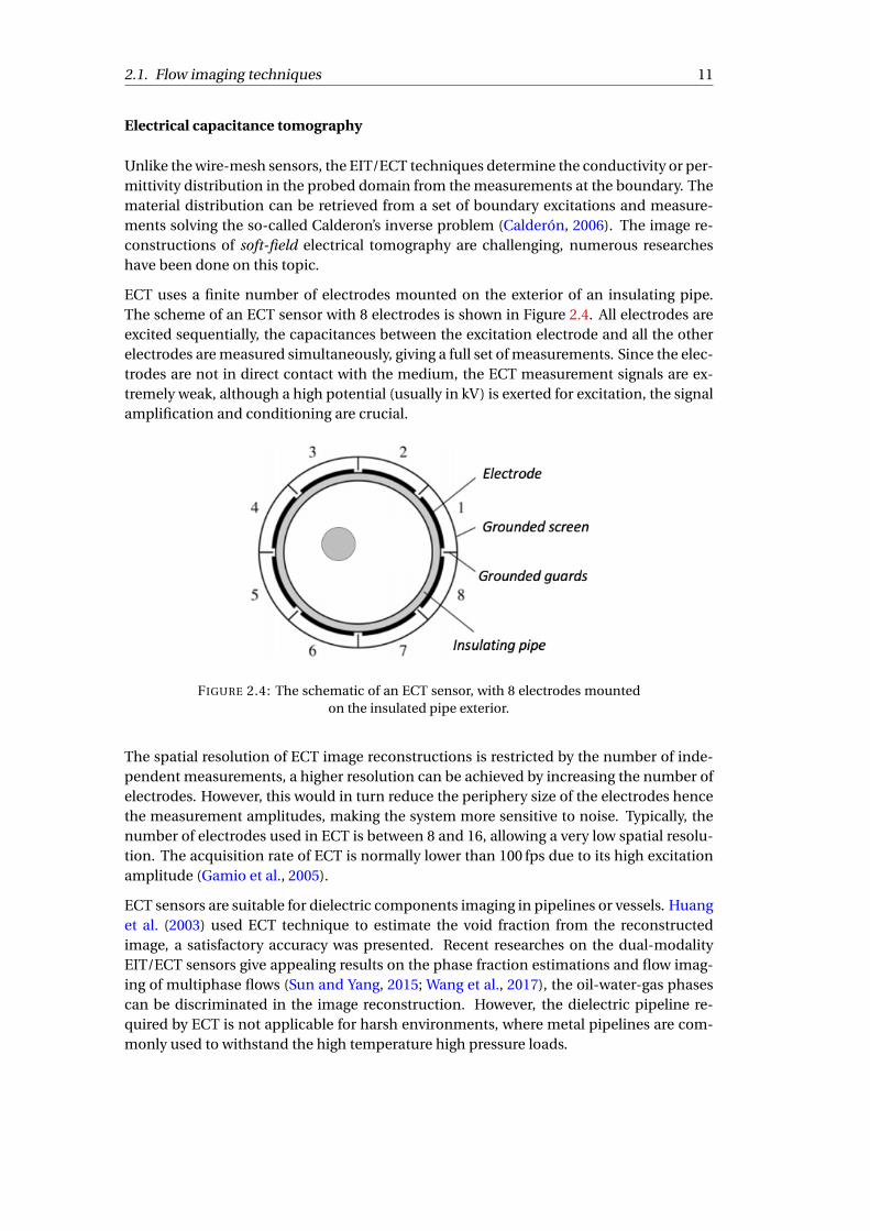
2.1.3 Electrical tomography
Electrical tomography techniques probe the domain based on the electrical properties ofmaterials. Unlike the radiation beams and the ultrasonic waves, the transmission path oflow frequency electric current evolves with the internal material distribution, featuring asoft-field nature. Various electrical tomography techniques have been developed and ap-plied for two-phase flow measurements, including the intrusive wire-mesh sensors, non-invasive ECT sensors, and non-intrusive EIT sensors.
Wire-mesh sensor
Wire-mesh sensor, by its name, uses a grid of wires to measure the flows in the studied do-main, it was firstly introduced in the pioneer work of Prasser et al. (1998). The principle isto use two sets of wires stretching along the pipe transverse section, which have small axialseparation in between and are perpendicular to each other, giving a grid of measurementpoints at their crossing points. During the measurement, the transmitters are activatedsequentially through multiplexing, the receivers are parallel sampled simultaneously. Awire-mesh sensor with 24£24 mesh grid is shown in Figure 2.3, the two sets of wires aretransmitters and receivers, respectively.
FIGURE 2.3: A wire-mesh sensor with a 24£24 measurement grid, adaptedfrom Nedeltchev et al. (2016).
Wire-mesh sensor allows to investigate multiphase flows at high spatial and temporal res-olutions, recently developed sensors feature an acquisition rate up to 10 kHz with a spatialresolution of around 3 mm (Wiedemann et al., 2019). It can provide information about lo-cal, cross-sectional or in-situ volume profiles and distributions of phases, however, it hasdisruptive effects on the flows. Yet, its application under harsh environment is challeng-ing, thicker wires are needed to ensure the robustness, which would in turn reinforce thedisruptive effects. Additionally, the fine grid of wires restricts the applications in flowswith solid particles or impurities, for example the flows in the hot leg of the PKL facil-ity. A good review of wire-mesh sensors applying into flow measurements under variousenvironments can be found in Peña and Rodriguez (2015).
2.1. Flow imaging techniques 11
Electrical capacitance tomography
Unlike the wire-mesh sensors, the EIT/ECT techniques determine the conductivity or per-mittivity distribution in the probed domain from the measurements at the boundary. Thematerial distribution can be retrieved from a set of boundary excitations and measure-ments solving the so-called Calderon’s inverse problem (Calderón, 2006). The image re-constructions of soft-field electrical tomography are challenging, numerous researcheshave been done on this topic.
ECT uses a finite number of electrodes mounted on the exterior of an insulating pipe.The scheme of an ECT sensor with 8 electrodes is shown in Figure 2.4. All electrodes areexcited sequentially, the capacitances between the excitation electrode and all the otherelectrodes are measured simultaneously, giving a full set of measurements. Since the elec-trodes are not in direct contact with the medium, the ECT measurement signals are ex-tremely weak, although a high potential (usually in kV) is exerted for excitation, the signalamplification and conditioning are crucial.
FIGURE 2.4: The schematic of an ECT sensor, with 8 electrodes mountedon the insulated pipe exterior.
The spatial resolution of ECT image reconstructions is restricted by the number of inde-pendent measurements, a higher resolution can be achieved by increasing the number ofelectrodes. However, this would in turn reduce the periphery size of the electrodes hencethe measurement amplitudes, making the system more sensitive to noise. Typically, thenumber of electrodes used in ECT is between 8 and 16, allowing a very low spatial resolu-tion. The acquisition rate of ECT is normally lower than 100 fps due to its high excitationamplitude (Gamio et al., 2005).
ECT sensors are suitable for dielectric components imaging in pipelines or vessels. Huanget al. (2003) used ECT technique to estimate the void fraction from the reconstructedimage, a satisfactory accuracy was presented. Recent researches on the dual-modalityEIT/ECT sensors give appealing results on the phase fraction estimations and flow imag-ing of multiphase flows (Sun and Yang, 2015; Wang et al., 2017), the oil-water-gas phasescan be discriminated in the image reconstruction. However, the dielectric pipeline re-quired by ECT is not applicable for harsh environments, where metal pipelines are com-monly used to withstand the high temperature high pressure loads.

12 Chapter 2. Introduction
Electrical impedance tomography
EIT uses a finite number of electrodes installed on the interior boundary of a studied do-main, making it an invasive but non-intrusive technique. Since the electrodes are in directcontact with the materials, a low excitation signal (several mA or V) is sufficient to give pre-cise measurements, featuring a safe and low cost system. Usually, alternating current orvoltage at a given frequency is used for excitation. The low excitation amplitude allows ahigh excitation frequency and high speed multiplexing, hence a high frame rate. Recentlydeveloped EIT systems can achieve up to hundreds or even thousands of fps using excita-tion frequencies from several to tens of kHz (Jia et al., 2017; Darnajou et al., 2020). Withthese advantages, EIT technique has been successfully applied in some cases of multi-phase flow monitoring and clinical imaging, among others.
A number of EIT systems dedicated to multiphase flow measurements have been devel-oped in the last two decades. A comprehensive review of EIT applications to various mediaand purposes in chemical engineering can be found in Sharifi and Young (2013). Specif-ically for two-phase flow measurements, George et al. (2000) presented an EIT systemapplied to solid-liquid and gas-liquid flows, the phase fractions within a circular cross-section were determined and compared with nominal values. Jia et al. (2017) developed avoltage source EIT system for highly conductive water-oil two-phase flow measurements,the cross-sectional tomographic images and axially stacked images were obtained, the to-tal phase fractions were estimated and compared to the reference values. Dupré (2017)developed an EIT system for void fraction estimation of two-phase flows, in which the so-called full-scan strategy was implemented, however, only static tests were carried out forsystem validation in their research.
Up to now, the main imaging techniques for multiphase flow measurements are presented,most of which show certain limitations for applications under harsh environments, wheremetal pipelines are inevitably used and impurities may present in the flows. In this con-text, EIT technique seems to bear encouraging features for flow measurements in suchcases.
2.2 Electrical impedance tomography
EIT technique determines the material distribution inside a 2D or 3D domain based ontheir constitutive electric properties, i.e. the electric admittivity (conductivity and permit-tivity). Certain current or voltage excitations and the resulting voltage or current measure-ments are performed on the boundary. In this section, the EIT mathematical basis andelectrode models are introduced, some practical aspects considered in implementation,e.g. excitation strategies and 3D effect, are discussed.
2.2.1 Forward model
Considering the electric field in a two- or three-dimensional domain ≠, from Maxwell’sequation, the electric potential u inside is governed by,
r ·°∞(x)rrru(x)
¢= 0, x in≠, (2.1)

2.2. Electrical impedance tomography 13
where ∞(x) = æ(x)+ i!≤(x) is the isotropic admittivity distribution in ≠, in which æ is theelectric conductivity, ≤ is the electric permittivity, ! is the excitation frequency. In mul-tiphase flow measurements, usually only the conductivity æ is considered, because theelectric permittivity ≤ of liquid phase can be neglected in the chosen working frequencyrange of EIT sensors (Dang et al., 2018a).
EIT forward problem is to compute the electrical field u inside the domain ≠ and theassociated boundary measurements from the knowledge of the conductivity distributionæ and the injecting current or voltage on the boundary. While the inverse problem is toestimate the conductivity profile æ in≠ knowing the injecting current/voltage and the re-sulting boundary measurements. Mathematically, infinite boundary excitations and mea-surements can be made on the boundary, determining a unique solution of the internalconductivity profile. In practice, the excitations and measurements can only be made ona finite set of electrodes on the boundary @≠ of the domain, defining a solution of finiteresolution. The EIT forward and inverse problems are commonly solved using Finite Ele-ment Method (FEM).
Figure 2.5 shows an EIT sensor with 16 evenly separated electrodes located on @≠. Here,the excitation currents are exerted on the electrodes i , j , the corresponding differencevoltages are measured at all the other electrodes simultaneously. Conventionally, the exci-tation signal is routed to one selected pair of electrodes at a given time (namely, one exci-tation pattern), then switched to the next pair, until all excitation patterns in one strategyare sequentially traversed (Cheney et al., 1999), forming a frame of measurement data.
FIGURE 2.5: Schematic of an EIT sensor with 16 electrodes (electrode in-dex is given from 1 to 16). The excitation currents are injected at electrodes
(i , j ), difference voltage is measured at neighboring electrodes.
The EIT problem is associated with an elliptic boundary-value problem prescribing Neu-mann boundary conditions, the Dirichlet boundary measurements depend on the inter-nal conductivity distribution. It aims at recovering the information on the admittivity dis-tribution inside a domain of interest from boundary measurements. The mathematicalbasis of EIT is introduced with the Neumann-to-Dirichlet (NtD) operator in the follow-ing section. Applying voltage excitation on the boundary defines the Dirichlet boundaryconditions, the associated forward problem gives the Dirichlet-to-Neumann (DtN) map,mathematically it is equivalent to the NtD map.

14 Chapter 2. Introduction
Neumann-to-Dirichlet map
The domain ≠ is assumed to be homogeneous except for a number of inclusions (orobjects), which are denoted as ≠i. These inclusions have a conductivity different withthe background, and they are assumed to be simply connected domains contained in≠. Specifically for two-phase flows, the conductivity of the water phase is within 10°4 °10°2S/m, and that of gas is around 10°15 °10°9S/m, i.e.,
æ=(
ª 0 in≠i,
1 in≠\≠i,(2.2)
with æ of the water phase normalized to 1.
Denoting as n the unit outward normal vector on the boundary @≠, which is assumed tobe smooth, we have the Neumann boundary conditions
ærrru ·n = f on @≠, (2.3)
in which f 2 L2(@≠) represents the boundary current density that satisfiesR@≠ f dS = 0.
Note that the model Eqn. (2.2) entails that ærrru ·n º 0 on the boundary @≠i of the inclu-sions.
Introducing the functional space H 1¶ (≠) = {' 2 H 1(≠) :
R@≠'dS = 0}, the Neumann bound-
ary value problem is as follows: find u 2 H 1¶ (≠) that satisfies
Z
≠ærrru ·rrr'dV =
Z
@≠f 'dS, 8' 2 H 1
¶ (≠). (2.4)
On denoting L2¶(@≠) = {' 2 L2(≠) :
R@≠'dS = 0}, the Neumann-to-Dirichlet (NtD) map, or
the so-called forward operator, is introduced as §æ : L2¶(@≠) ! L2
¶(@≠) so that the bound-ary potential can be written as §æ f = u|@≠, where u 2 H 1
¶ (≠) is the solution to Eqn. (2.4).The boundary potential can be measured and compared with the boundary potential§0 f = u0|@≠ for the same f and ≠ but without inclusions, i.e. ≠i = ;, with u0 2 H 1
¶ (≠)being the solution of:
Z
≠rrru0 ·rrr'dV =
Z
@≠f 'dS, 8' 2 H 1
¶ (≠), (2.5)
which corresponds to the reference problem with a homogeneous conductivity distribu-tion inside the domain ≠. The relative NtD map is denoted as ¶ = §æ°§0. In the studyby Hanke and Brühl (2003), the eigenvalues of ¶ are used to locate the inhomogeneitiesnon-iteratively.
Electrode models
In practical implementation, the boundary current density f cannot be measured, onlythe current or voltage at discrete electrodes could be obtained. There are various electrodemodels available depending on their assumptions on current density, i.e. the gap model,the shunt model and the complete model (Cheng et al., 1989; Wang, 2005).
The gap model assumes that the current density is constant over electrodes, while theshunt model considers that the integral of the current density over the electrode equalsto the total current flowing through that electrode. Furthermore, the complete model

2.2. Electrical impedance tomography 15
is based on the shunt model, but takes into account the electrochemical effect at theinterface between the electrode and the probed medium, which is called the ‘contactimpedance’. Compared to the gap model, the shunt and complete models are closer toreality (Cheney et al., 1999).
In the shunt model, considering a number ` of identical electrodes placed on @≠ equallyspaced, the integral of the current density over the electrode is equal to the current throughthis electrode, while the current density at the isolated gaps between electrodes is zero, i.e.
Z
ek
ærrru ·n ds = Ik for k = 1, . . . , ` (2.6)
ærrru ·n = 0 on @≠\[k
ek , (2.7)
where Ik is the current passing through the kth electrode and ek is the surface of the kth
electrode. Besides, the electrodes are assumed to be perfectly conducting so that the elec-trostatic potential u|ek is constant at each electrode.
EIDORS code
In current study, the MATLAB based Electrical Impedance Tomography Diffusion basedOptical Tomography (EIDORS) (Polydorides and Lionheart, 2002) code is employed tosolve both the EIT forward and inverse problems using FEM. The goal of EIDORS is pro-viding free software algorithms for forward and inverse modeling for EIT in medical andindustrial settings, and to share data and promote collaboration between groups workingon these fields. A number of pre-defined functions are available in EIDORS to solve theEIT forward and inverse problems conveniently (Adler and Lionheart, 2006).
Typically, the procedures to solve an EIT forward problem are as follows: i) define a 2Dor 3D studied domain using certain geometry parameters, as well as the excitation andmeasurement strategies; ii) generate a finite element mesh with proper parameters, pos-sibly refine the mesh near the boundary of the domain especially the electrodes; iii) as-sign the conductivity profile to the mesh; iv) solve Eqn. (2.1) with the associated bound-ary excitations using FEM, the potential field and boundary measurements can be ob-tained. EIDORS has a bunch of pre-defined forward models incorporated in the func-tion mk_common_model. User-defined forward models and electrode configurations canbe realized conveniently by calling external codes, e.g. the Netgen or Gmsh, to generatemesh on complex geometries. The excitation and measurement strategies are designatedwith the function mk_stim_patterns, commonly applied strategies are pre-defined. Theelectrode contact impedance can be modified easily, making it possible to apply differentelectrode models. The conductivity profile is assigned simply setting a value to the cor-responding mesh element. Finally, the prescribed forward model is saved in a MATLABobject, the electrical field in the domain and the boundary measurements are computedusing FEM solvers provided by fwd_solve function, both the first-order and the second-order solvers are available.
For EIT inverse problem, EIDORS facilitates 2D and 3D image reconstructions with built-in functions implementing various iterative and non-iterative methods, mainly in leastsquares sense. Various image reconstruction methods and their implementations in EI-DORS will be further discussed in Chapter 5.

16 Chapter 2. Introduction
Furthermore, EIDORS provides several functions for model visualization. The show_femfunction allows to visualize a 2D or 3D finite element model with the values in the meshelements, the show_slice function gives a slice of the model at a given plane. The potentialand current fields, as well as the sensitivity distributions can be easily superimposed onthe finite element model for visualization.
2.2.2 Excitation strategy
Considering the conditions to be imposed on the currents/voltages fed into the electrodesand their measurement counterparts, they may be chosen arbitrarily and can be classi-fied into pair and multiple drive systems depending on the number of excitation carryingelectrodes that are active at a given time. In a pair drive system, the excitation is appliedthrough a pair of source and drain electrodes. In a multiple drive system, all of the elec-trodes are active simultaneously. In any case, the specific form of the boundary conditionconsidered defines an excitation pattern. A given series of excitation patterns is appliedsequentially, forming an excitation strategy, which is ultimately used to compute a tomo-graphic image.
Among the preeminent excitation strategies available and easily implementable with up-to-date hardware, the adjacent, opposite, full-scan (Dupré et al., 2017a), and trigonomet-ric strategies (Cheney and Isaacson, 1992) have shown satisfying performances and beenstudied further in the present work. Their schematics are shown in Figure 2.6, the detailedintroduction is presented hereafter.
FIGURE 2.6: Schematics of the four excitation strategies, the blue dottedlines in (a) to (c) indicate the following electrode pairs for excitation. In(d) the trigonometric function with a frequency j = 4 is plotted, giving the
excitation amplitude at each electrode.
Pair drive systems
Adjacent strategy. It is defined by the pattern where the excitation current is injectedat two neighboring electrodes. In the adjacent strategy, the current is switched to thenext pair of neighboring electrodes until all the possible neighboring pair have been con-sidered. The number Ne of excitation patterns is equal to the number of electrodes, i.e.Ne = `, yielding a number of measurements Nm = `2 . The main drawback of the adjacentstrategy is the expected non-uniformity of the current distribution within the domain,with the current density being maximized in a neighborhood of the excitation electrodesand much lower at distant electrodes, thus leading to measurements of low amplitude atthe latter, which would therefore be more susceptible to noise pollution.

2.2. Electrical impedance tomography 17
Opposite strategy. It considers current injection at pairs of opposite electrodes, withNe = `/2 possible excitation patterns, which gives Nm = `2/2 measurements. The lattervalue is half this associated with the adjacent strategy, which can be expected to be detri-mental to the images to be reconstructed. Nonetheless, the signal amplitudes acquired atdistant electrodes can be expected to be larger in the opposite strategy compared to theadjacent one, as the maximal distance between excitation and measurement electrodesbeing approximately reduced by a factor
p2 for the former.
Full-scan strategy. Here, all electrodes are sequentially selected to be source and drainuntil all possible pairs of electrodes have been formed, giving Ne = `(`°1)/2 and Nm =`2(`° 1)/2. This strategy includes the excitation patterns of the adjacent and oppositestrategies, among others, thus leading to comparatively longer acquisition times. Indeed,it respectively involves (`°1)/2 and (`°1) times more patterns than the latter.
Multiple drive systems
Among the possible excitation strategies applicable to multiple drive EIT systems, we onlyfocus here on the following one which seems to be favored by previous studies.
Trigonometric strategy. This strategy has been introduced in the search for an optimalexcitation pattern and it has been shown to maximize a distinguishability criterion, seeCheney and Isaacson (1992). In each excitation pattern, the current at the electrodes ek ,for k = 1, . . . ,`, is constructed from a cosine or sine function of varying angular frequency! j = 2º j /`, as
Ik, j =(
I0 cos(k! j ) with 1 ∑ j ∑ `/2,
(°1)k+1I0 sin(k! j ) with `/2 < j ∑ (`°1),(2.8)
where I0 is a fixed amplitude. The definition (2.8) of Ik, j is to be used in the boundarycondition (2.6) and it can be adapted to the case of voltage excitations. This defines Ne =(`°1) different patterns that lead to Nm = `(`°1) measurements overall. Compared tothe other strategies, the trigonometric one requires simultaneous excitation of multiplesources, which is more demanding in practice and increases the complexity of the EITsystem.
For conciseness, the latter will only be described in terms of current excitation and volt-age measurement, alternative operating modes available are shown in Figure 2.7. Thecurrent-based operating mode can easily be transformed into a voltage-based mode forboth excitations and measurements. With the resistor having fixed value R0 connected tothe electrode, the excitation or measurement current can be calculated from the voltagemeasurement across the resistor. The operating mode (b) has been applied in several EITsystems, such as the ProME-T system (Dupré et al., 2017a), and the system developed inJia et al. (2017) for highly conductive oil-water two-phase flow measurement. The ONE-SHOT EIT system reported recently in Darnajou et al. (2020) applies the operating mode(c). Both the ProME-T and ONE-SHOT systems have been used in the present thesis workfor static and dynamic experiments, separately.

18 Chapter 2. Introduction
(a) (b) (c)
FIGURE 2.7: Schemes of EIT operating modes: (a) Current excitationat electrodes (i , j ) with difference voltage measurements at neighboringelectrodes; (b) Voltage excitation at electrodes (i , j ) with difference voltagemeasurements at neighboring electrodes; (c) Voltage excitation at elec-
trodes (i , j ) with voltage measurement across R0 at each electrode.
Number of independent measurements
The number N im of independent measurements accessible in each strategy is vital, as it
determines the spatial resolution of the reconstructed images produced and might not benecessarily equal to the number Nm of measurements. Since source and drain are essen-tially the same for pair drive strategies, the measurements would be reciprocal for a spe-cific pair of electrodes. For an EIT system with ` electrodes, Breckon and Pidcock (1988)showed that, for any pair drive strategy, the number N i
m of independent measurement isat most equal to `(`°1)/2. Yet, the opposite strategy is such that N i
m = `(3`°2)/8 becauseit makes use of a relatively limited number of excitation patterns.
Particularizing for an EIT system with ` = 16 electrodes, Table 2.1 provides the numberN i
m of independent measurements and the ratio with the number Nm of measurementsfor the various excitation strategies considered. This ratio is called the redundancy ratio,as it quantifies the redundancies in the measurements, with the value 1 being attained ifthey are all independent. Conversely, a small ratio characterizes large measurements re-dundancies, which may be a factor to be considered if memory and computational powerare an issue.
TABLE 2.1: Number N im of independent measurements and redundancy
ratio relatively to the number Nm of measurements for the various strate-gies, considering an EIT system with 16 electrodes.
Strategies Adjacent Opposite Full-scan Trigonometric
N im 120 92 120 240
N im/Nm 0.47 0.72 0.06 1
Up to now, most of the practical EIT systems in use applied the adjacent excitation strat-egy due to its simplicity in implementation, only requiring a pair of sources and a fewmultiplexing operations. While the other excitation strategies have proven to be effectiveand easy to implement using modern hardwares. Some studies involving physical model-ings and numerical simulations have been done on these excitation strategies before. Inthe present thesis work, the four excitation strategies considered here have been assessedon a number of criteria in terms of practical implementation and quality of reconstructedimages, aims at confronting some of the predominant EIT excitation protocols on prac-tical systems that is dedicated to the imaging of media with highly contrasted material

2.2. Electrical impedance tomography 19
components, for example, two-phase flows. The results will be shown in Section 3.2 and5.3.
2.2.3 3D effect
Due to the soft-field nature of electrical current and the finite length of electrodes, theelectric field in the studied domain spreads far beyond the electrode plane, leading to a3D sensing region for a 2D sensor. The objects outside of the electrode plane would haveeffects on the measurements hence on the reconstructed images, which is known as the3D effect of EIT. Also, severe distortions of the electric field appear on both ends of theelectrodes, giving the so-called ‘fringe effect’ (Sun and Yang, 2014).
2D simulations have been carried out to explain the geometrical spreading effect of EIT.The open source code FreeFem++ (Hecht, 2012) is used to solve the EIT forward problem.FreeFem++ is a partial differential equation solver for multi-physics non linear systemsin 2D and 3D. Here, the simulation model is set to be a rectangular with unit height anda width of 2. A pair of electrodes on the opposite boundaries are considered, the restof the boundaries are insulating, i.e. zero current density. The generated finite elementmesh is refined on the electrodes, an example mesh for the case with Le = 1.2 is shownin Figure 2.8. Voltage sources with amplitudes of ±1 V are exerted on the two electrodesrespectively, the potential and current fields inside the domain are computed for variouslengths Le of the two electrodes.
FIGURE 2.8: An example finite element mesh for the case with Le = 1.2.
Figure 2.9 shows the current streamlines and equipotential lines in the domain for caseswith electrode length Le = 0.02, 0.2, 0.7, and 1.2, separately. The vectors in blue representthe current streamlines, and the contours with different colors for equipotential lines. Aswe can see, in all cases the current streamlines concentrate in the middle of the domain,and the axial extends of the high concentration region is similar for different Le . Con-sidering the case Le = 0.02, the current streamlines spread out far beyond the electrodeplane, the geometrical spreading effect of EIT is clearly shown. Noting that the currentstreamlines are computed from local potential gradient, intensive streamlines indicate ahigh potential gradient, where a small conductivity change can have strong effect on thepotential field. As Le increases the current streamlines between the two electrodes be-come more homogeneous, indicating a smoother potential field, which may give a morehomogeneous sensitivity distribution. In addition, the fringe effect is presented by theextraordinarily uneven current streamlines at the ends of the electrodes, see Figure 2.10.

20 Chapter 2. Introduction
(a) Le = 0.02. (b) Le = 0.2.
(c) Le = 0.7. (d) Le = 1.2.
FIGURE 2.9: The current streamlines and equipotential lines in the do-main with varying electrode lengths Le = 0.02, 0.2, 0.7, 1.2.
FIGURE 2.10: Zoom-in plot of the current streamlines at the ends of theelectrode for Le = 0.2.
Besides, a number of researches have been done studying the effects of guarding elec-trodes on the potential and current fields inside the domain (Ma et al., 1997; Plonsey andCollin, 1977). This approach employs extra planes of electrodes aside the main plane,take Figure 2.11(a) as an example, the pair of electrodes in the middle represent the mainplane, while the other two pairs of electrodes are called the ‘guarding electrodes’, they canbe either grounded or excited by the same voltage sources as the main plane electrodes(Ma et al., 1997).
A series of simulations have been performed with different distances Ld between the guard-ing electrode plane and the main plane. The electrode length is fixed as Le = 0.2, the cur-rent streamlines inside the domain for Ld = 0.3 and Ld = 0.7 are computed and plotted.

2.2. Electrical impedance tomography 21
(a) Ld = 0.3. (b) Ld = 0.7.
FIGURE 2.11: The current streamlines and equipotential lines in the do-main for Le = 0.2 and Ld = 0.3, 0.7, the guarding electrodes are excited
with the same voltages as the main plane electrodes.
(a) Ld = 0.3. (b) Ld = 0.7.
FIGURE 2.12: The current streamlines and equipotential lines in the do-main for Le = 0.2 and Ld = 0.3, 0.7, the guarding electrodes are grounded
(at zero potential).
Figure 2.11 shows the results where the guarding electrodes are excited by the same volt-ages as the main plane electrodes, while Figure 2.12 shows that with grounded guardingelectrodes (zero potential is exerted). As we can see, despite the local changes taking placenearby the electrodes, the axial extend of the high concentration region of the currentstreamlines is not constrained by the guarding electrodes for both cases, on the contrary,the extend is even enlarged in cases with Ld = 0.7. Besides, comparing the current stream-lines between the main plane in Figure 2.9(b) and 2.11(b), it is interesting that the excitedguarding electrodes may flatten the current streamlines comparing to the case withoutguarding electrodes, which may bring some benefits diminishing the inhomogeneous ofEIT sensitivity distribution.
Although some researches argued that the guarding electrodes does not fulfill the expec-tation that it reduces the geometrical spreading effect (Plonsey and Collin, 1977), theymay bring some advantages, such as a more homogeneous sensitivity distribution anda stronger measurement signals. Furthermore, the use of multiple planes of electrodesmay favor 3D image reconstructions: exploiting the excitations on the electrodes of differ-ent planes, the sensitivity in the center of the sensing domain may be improved. Severalcross-plane excitation patterns have been studied in Wagenaar and Adler (2016), provingthe advantages of multiple electrode planes in 3D image reconstructions.


23
Chapter 3
EIT system design for two-phase flowimaging
The aim of two-phase flow measurement is to estimate (online or offline) various param-eters of the flow, including the phase distribution, the cross-sectional or volumetric phasefraction, the flow pattern, among others. These information are vital to assess the flowinstability and heat transfer coefficient. To fulfill the expectations, the EIT systems dedi-cated to two phase flow measurements should be designed to have adequate spatial andtemporal resolutions, and be robust to measurement noise.
In this chapter, the EIT systems used in the present thesis study, namely the ProME-T andONE-SHOT systems, are briefly introduced. Then, the four excitation strategies presentedin Section 2.2.2 are compared regarding several practical implementation criteria. After-wards, the influences of electrode size on the system performance are studied applyingtwo sets of electrodes with different sizes into the ProME-T system, with respect to theimpedance response, noise level, and residual error induced by multiplexing. The resultsare considered in the design of a dual-plane test section for the PKL facility.
3.1 EIT systems developed in LTHC
A practical EIT system consists of hardwares and software. Typically the hardwares in-clude: i) a data acquisition system to generate the excitation signals and measure theboundary voltages/currents; ii) a multiplexer routing the excitation signals to the selectedelectrodes, possibly through Time Division Multiplexing (TDM) or Frequency DivisionMultiplexing (FDM); iii) a Printed Circuit Board (PCB) handling the operating mode ex-plained in Figure 2.7, commonly the multiplexer is also mounted on the PCB for optimalperformance, sometimes with the signal filter and amplifier; iv) a test section with certainnumber of electrodes; v) auxiliary devices for input/output and proper wires to connectall components together. In terms of the software, a data acquisition code is required tomanage the multiplexing, data logging and possible online display; also, proper data post-processing codes should be developed to handle the measurement data, for further imagereconstruction and flow features extraction. Here, we focus on the hardwares, the softwarewould be investigated in the latter chapters.
Two EIT systems have been developed in LTHC based on the TDM and FDM separately,i.e. the ProME-T system developed in Dupré (2017), and the ONE-SHOT system developedin Darnajou et al. (2020). Both of them implement the full-scan excitation strategy usingvoltage sources, their system specifications, realization procedures and data processingmethods are described as follows.

24 Chapter 3. EIT system design for two-phase flow imaging
3.1.1 ProME-T system
Hardwares
The ProME-T system was developed in Dupré (2017) for the purposes of two-phase flowmeasurement and phase fraction estimation, while only static experiments were accom-plished for system validation. The main components of the system are shown in Fig-ure 3.1. It has 16 electrodes on the internal boundary of a PMMA test section, with anangular separation of 22.5±. The signal excitation and acquisition are both realized by theNational Instrument PXI-6368e card (PXIe, 2016), which has four Analogue Output (AO)channels at a sampling rate up to 3.33 MHz, and 16 differential Analogue Input (AI) chan-nels up to 2 MHz. The operating mode in Figure 2.7(b) is implemented in ProME-T, theexcitation signals are alternating voltages with an amplitude of ±1 V to avoid the elec-trolysis reaction of water. For each excitation pattern, the difference voltages between allneighboring electrodes are measured simultaneously. The excitation current is calculatedfrom the voltage measurement across the constant resistor R0 connecting to the excitationsource, with R0 = 200≠ in the present system.
FIGURE 3.1: Left: the ProME-T system in LTHC applying TDM with 16electrodes. Right: the two sets of electrodes with different lengths avail-
able for ProME-T.
The full-scan strategy is implemented in the ProME-T, giving 120 different excitation pat-terns. A 16 ports multiplexer is mounted on the PCB to perform TDM, routing the excita-tion signals to the selected pair of electrodes for each excitation pattern. The addresses ofthe source and drain electrodes are assigned to the multiplexer by the eight Digital Output(DO) channels of the PXIe card, four channels for each.
The test section is a cylinder pipe with diameter of 51 mm and height of 270 mm, the elec-trodes are designed to be removable. Two sets of electrodes with different sizes are avail-able: the Electrode Set 1 (ES1) of size 154 mm£4 mm and the Electrode Set 2 (ES2) of size5 mm£4 mm, as shown in Figure 3.1. The connections between the electrodes and thePCB are realized by the co-axial wires and Bayonet Neill-Concelman (BNC) connectors, toreduce the electro-magnetic distortion.

3.1. EIT systems developed in LTHC 25
The speed of two-phase flows can be up to 10 m/s during the measurement, a high ac-quisition rate is always advantageous, however, high frequency electronic operations mayinduce extra electrical noise to the measured signal. The typical frame rate of the ProME-Timplementing the full-scan strategy is 208 fps, which is a compromise between the acqui-sition rate and measurement accuracy.
Equivalent circuit model
Considering the operating mode of the ProME-T system, the measurement system at eachexcitation pattern can be assumed as a closed circuit shown in Figure 3.2, where V0 repre-sents the excitation voltage, the combination of the charge transfer resistance Re and thedouble layer capacitance Ce contributes to the electrode-electrolyte contact impedance,here it represents the summation of the contact impedances at the source and drain elec-trodes, Z is the bulk impedance of the medium. They are connected in a cascade way withthe constant resistor R0. The current IZ passing through the circuit can be calculated fromIZ =VR /R0, with VR the voltage measurement across R0.
FIGURE 3.2: Closed circuit between the source and drain electrodes foreach excitation pattern.
The total impedance Z tot of the system is
Z tot = Z sour ce +Z dr ai n +Z +R0 =V0/IZ , (3.1)
with Z sour ce and Z dr ai n the contact impedances at the source and drain electrodes, theyare electrode-specific and invariant with the phase distributions inside the domain, thuscan be calculated and excluded from the closed circuit, giving the bulk impedance Z .
Clearly, Z evolves with the phase distribution and the excitation electrodes, while it is alsoaffected by the frequency of the excitation signals, so do the Z sour ce and Z dr ai n . Dupréstudied the frequency response of the total impedance Z tot between two point-like elec-trodes located on the opposite of a pipe, using a homogeneous electrolyte of differentconcentrations as the conductive medium, the results are presented in Dupré (2017, Fig-ure 2.29 and 2.30). It is shown that at medium excitation frequencies (typically from 1 kHzup to 100 kHz), the total impedance is mainly real: the bulk impedance dominates theglobal impedance while the electrode contact impedance is not significant. In currentstudy, the frequency responses of the total impedances using the two sets of electrodeshave been investigated, the results are shown in Section 3.3.

26 Chapter 3. EIT system design for two-phase flow imaging
Measurement data processing
As mentioned, the excitation signal used in the ProME-T is sinusoidal wave of specificfrequency, which is sampled Nsp times for each period. In each excitation pattern, Np pe-riods of excitation signal are held on the selected electrodes, meanwhile, boundary mea-surements are taken simultaneously on all the `= 16 AI channels. A frame of acquisitionis composed by Ne excitation patterns of one excitation strategy, giving (Nsp £Np £Ne )£`measurements. Typically in ProME-T, Np = 2 and Nsp = 20 are taken, yielding ª 600 kB ofmeasurement data with double precision for one frame.
During data post-processing, Fast Fourier Transform (FFT) is performed on every Np£Nsp
data points for each channel, the amplitude at excitation frequency corresponds to themeasurement of an excitation pattern. In the present thesis study, the image part of theamplitude is not considered, the real part is taken as the fundamental signal. The datasize after FFT is reduced to Ne£`, it will be further used in the eigenvalue-based approachpresented in Chapter 4, and in the image reconstructions discussed in Chapter 5.
3.1.2 ONE-SHOT system
Hardwares
The logic of EIT hardware design has been mature for decades now and recent advanceshave focused on greater accuracy, faster acquisitions and the ability to apply parallel multi-frequency excitations (Aguiar Santos et al., 2016). Recently, an innovative concept ONE-SHOT has been proposed in Dupré and Mylvaganam (2018), in which the FDM is used todiscriminate some superimposed signals at multiple frequencies, giving access to bound-ary measurements of multiple excitation patterns simultaneously. It is applicable to bothpair drive and multiple drive systems avoiding the need of multiplexing.
The principle of ONE-SHOT method is to assign a specific frequency to the excitation sig-nal of each excitation pattern. The superimposed excitation signals are injected to thecorresponding electrodes simultaneously, with the resulting boundary voltages measuredat the same time. The boundary measurements are discriminated through FFT, to obtainthe measurement amplitude for each excitation pattern. That is, in FDM the multiplexingis not accomplished physically, but mathematically through FFT. According to the Nyquistcriterion, the measurement sampling frequency should be at least double of the highestexcitation frequency to correctly reconstruct the amplitudes of all excitation frequencies.Thus, the number of sampling points acquired for one frame is Nd = nextpowerof2(2Ne )at the minimum to discriminate the signals, which is the next number over 2Ne that is thepower of 2, to ease the FFT computation. Considering the sampling rate Sm of the dataacquisition module, the maximum frame rate can be up to Sm/Nd fps.
The ONE-SHOT method has been implemented in Darnajou et al. (2019, 2020) with `= 16electrodes, the developed system is shown in Figure 3.3. The system employs the CRIO-9039 module (cRIO, 2018) as the controller, it has eight ports for AI/AO modules with asampling rate up to 1 MHz, with which the excitation signals generation and data acquisi-tion are realized. The full-scan strategy implemented requires a Nd > 240, supporting anultra-high frame rate up to 3906 fps.
The operating mode shown in Figure 2.7(c) is implemented, a PCB board is designed toconnect each electrode with a constant resistor R0 = 100≠. Again, the co-axial wiresand BNC connectors are used to connect the electrodes to the PCB. The test section is

3.1. EIT systems developed in LTHC 27
FIGURE 3.3: The ONE-SHOT system developed in LTHC using FDM with16 electrodes, adapted from Darnajou et al. (2020).
a PMMA pipe with diameter of 80 mm and height of 336 mm, it has 32 electrodes of size150 mm£6 mm on the boundary, allowing possible upgrade of the present system.
Equivalent circuit model
The equivalent closed circuit model of the ONE-SHOT system for each excitation patternis shown in Figure 3.4, which is similar to that of the ProME-T system but with an ex-tra R0. Considering the current measurements at all electrodes meet the zero summa-tion (see Eqn. (2.4)), the current IZ flowing through the closed circuit can be calculatedby IZ = °(
PNse=1 Vs)/R0, where
PNse=1 Vs represents the summation of the voltage measure-
ments at the electrodes other than the exciting ones. Moreover, Darnajou et al. (2020)showed that the effect of contact impedance is eliminated in the ONE-SHOT system dueto the continuous excitation signal, i.e. Z sour ce = Z dr ai n = 0. Finally, the total impedanceis calculated directly by Z tot = Z +2R0 =V0/IZ .
FIGURE 3.4: Equivalent closed circuit of the ONE-SHOT EIT system.
Measurement data processing
As explained, Nd data points are acquired at each measurement channel for one frame ofacquisition, giving Nd£`data points in total. The measured data contains the information

28 Chapter 3. EIT system design for two-phase flow imaging
at Ne excitation frequencies to be retrieved through FFT. Benefiting from the Field Pro-grammable Gate Array (FPGA) incorporated in the controller, the FFT of the acquired datacan be computed almost simultaneously with data acquisition, giving the correspondingamplitude for each excitation pattern in frequency domain, so that the raw measurementsignals can be discarded, only the fundamental amplitude at each excitation frequencyare saved, giving a data size of Ne £` for one frame. Finally, the data saved to the localhost in the ONE-SHOT system is Np £Nsp times less than in ProME-T, facilitating the datalogging for ultra-high speed EIT (several thousands of fps).
3.2 Practical comparison of excitation strategies
The excitation strategy is one of the key aspects one have to choose prior to EIT systemdesign. On one hand, it determines the number of AO channels required and the multi-plexing sequence in the data acquisition code. On the other hand, it has strong effects onthe boundary measurement responses and sensitivity distribution in the probed domain,hence on the reconstructed images.
There has been an intensive search for optimal current patterns (or excitation strategies ina general sense), starting in the field of medical imaging in the 1990s. Gisser et al. (1987) in-troduced the concept of distinguishability as a quantitative criterion to evaluate the qual-ity of a current pattern. It is defined as the quantity ±d = kVs °V0k2
L2 /kIek2L2 , where Vs
and V0 are the boundary voltage measurements associated with the studied and referenceconfigurations, given the current excitation Ie . Cheney and Isaacson (1992) proved ana-lytically that the trigonometric pattern maximizes ±d . However, the use of an alternativecriterion may lead to a different optimal current pattern. For example, if the total injectedcurrent is constrained, then it has been shown in Lionheart et al. (2001) that the optimalcurrent pattern turns out to be the pair drive pattern. Furthermore, Demidenko et al.(2005) deployed a criterion that quantifies the accuracy of the reconstructed tomographicimages, based on the total variance of the estimated resistance (or conductance) matrix,and developed an adaptive approach with real-time updating of the current pattern.
The optimal current patterns described above have been investigated in depth mathe-matically. Yet, there is a lack of a systematic comparison of these physical and numericalmodels using actual experimental data and indicators of the quality of reconstructed im-ages, which is the ultimate goal of tomography. Clearly, there is not a consensus on theoptimal current pattern to be used, but most of the practical systems in use employ theadjacent pattern (Dickin and Wang, 1996; Sun and Yang, 2015; Jia et al., 2017) with theadvantage of easy implementation, although it is considered to be harmful to distinguishchanges in internal conductivity distributions (Adler et al., 2011).
The four excitation strategies presented in Section 2.2.2 have their own pros and cons butlack exhaustive comparisons in practical set-ups. Up to the author’s knowledge, only theadjacent and opposite strategies were compared in terms of reconstruction performancesin Stephenson et al. (2008). In the present thesis study, the adjacent, opposite, full-scanand trigonometric strategies have been compared comprehensively in terms of (i) feasi-bility of the hardware implementation, (ii) amplitude of the measurement responses, (iii)sensitivity distribution, and (iv) quality of the reconstructed images. The results of thefirst three aspects are presented in this section, as of the last aspect will be described inSection 5.3.

3.2. Practical comparison of excitation strategies 29
3.2.1 Representative frame rates
To begin with, typical EIT architectures and some estimations of the representative acqui-sition frame rates for each strategy (a frame being composed of the acquisitions associatedwith all of its excitation patterns) are presented with `= 16 electrodes.
TDM systems
For pair drive excitations, the TDM systems generally use a multiplexer to switch the sig-nals to the selected pair of source and drain electrodes. For such systems, the transientphases during multiplexing have been shown to be harmful to the measurements, in par-ticular due to the contact impedance, see Wang (2005). Therefore, the measurements per-formed at the excitation carrying electrodes are generally discarded. However, it has beenevidenced in Dupré (2017) that the residual error induced by multiplexing could be ne-glected when employing an appropriate switching approach and large electrode area. Inthe present study, all measurements are taken into account when considering pair driveexcitations.
For the multiple drive trigonometric strategy, the multiplexing is not needed since eachelectrode is directly connected to an individual electrical source whose amplitude varieswith the excitation pattern. Nonetheless, with the requirement to control all of these indi-vidual sources, the system becomes more complex.
Here, the ProME-T system is taken as a prototypical example, to estimate the associatedframe rates for the various excitation strategies, see Table 3.1. Using ProME-T, the typi-cal frame rate for the full-scan strategy is 208 fps. Recalling the number Ne of excitationpatterns of various strategies in Section 2.2.2, the typical frame rates for the adjacent andopposite strategies would be 1560 fps and 3120 fps, respectively. Lastly, for the trigonomet-ric strategy, three more PXIe cards are required to drive excitation signal at each electrode,which therefore bear an extra cost. The resulting frame rate is estimated at 1664 fps.
FDM systems
In FDM systems, the excitation signals of all excitation patterns in one strategy are su-perimposed and exerted to corresponding electrodes simultaneously, with the boundarymeasurements taken at the same time. The frame rate is only relevant to the number Nd ofsampling points acquired at each measurement channel in one frame, as explained in Sec-tion 3.1.2. Taking the ONE-SHOT system as a prototypical example, the maximum framerate is 106/Nd fps for all excitation strategies. Considering the Ne of various strategies, theestimated frame rates are provided in Table 3.1. It is underlined that even for pair drive ex-citation strategies, the FDM systems require 14 extra electrical sources than conventionalsystems.
TABLE 3.1: Estimated acquisition frame rates (fps) for the excitationstrategies considered and using EIT systems with 16 electrodes.
Strategies Adjacent Opposite Full-scan Trigonometric
ProME-T 1560 3120 208 1664ONE-SHOT 31250 62500 3906 31250

30 Chapter 3. EIT system design for two-phase flow imaging
3.2.2 Statistics of measurement amplitudes
Due to the ill-posedness of the EIT inverse problem, even a small measurement noise canlead to large discrepancies in the reconstructed images. Thus, in practice, additionally tothe number N i
m of independent measurement discussed previously, it is also insightfulto evaluate the statistical distributions of the measurement amplitudes at different elec-trodes for various excitation strategies. Specifically, the mean and standard deviation ofsynthetic boundary measurements are computed, which give a hint on the robustness ofvarious excitation strategies to measurement noise.
FIGURE 3.5: 2D forward simulation model with 16 evenly spaced elec-trodes.
These are investigated based on numerical simulations using EIDORS. An EIT model isbuilt with the homogeneous background conductivity and compute a set V of boundarymeasurements for each excitation strategy, as shown in Figure 3.5. The domain is set tobe a 2D disk with unit radius and 16 evenly spaced electrodes with peripheral width equalto 0.16, which coincides with the experimental test section of ProME-T system introducedin Section 3.1.1. A triangle mesh with 8791 nodes is used in the FEM model. For eachstrategy one considers a current source of unit amplitude. The mean (average amplitude)and the standard deviation (spatial variability) computed for each measurement set V arereported in Table 3.2.
TABLE 3.2: Mean and standard deviation of the boundary measurementsfor the various excitation strategies and a 16 electrodes EIT system.
Strategies Adjacent Opposite Full-scan Trigonometric
Mean (V) 0.1931 0.3220 0.2817 0.8067Standard deviation (V) 0.3915 0.2668 0.3130 0.3352
For pair drive systems, the adjacent strategy is characterized by the lowest mean and thehighest standard deviation, and conversely for the opposite strategy. The full-scan is asso-ciated with intermediate values. Indeed, the adjacent strategy has much lower measure-ment amplitudes at electrodes away from the source electrodes, which are more distanton average compared to the opposite strategy. The full-scan strategy contains the exci-tation patterns of the two previous strategies among others. For multiple drive systems,considering the trigonometric strategy yields measurements of a much larger amplitudein average compared to pair drive systems, since it inputs more power into the systemwith all electrodes being active in each pattern. Moreover, the measurements standarddeviation is comparable to the full-scan strategy.

3.2. Practical comparison of excitation strategies 31
3.2.3 Sensitivity distributions
The effectiveness of each internal region contribution to the overall measurement signalis assessed numerically through the sensitivity maps for each strategy. Kauppinen et al.(2006) visualized such sensitivity distributions for the adjacent and opposite strategies,and also the so-called cross and adaptive ones, but it was for single excitation patternsrather than for the global excitation strategies that we consider here.
Given an EIT system, a localized conductivity perturbation ±æwithin the probed mediumcan induce a perturbation ±u of the electric potential, which can in turn be measuredon the boundary. For a certain excitation strategy, the greater the perturbation ±u, themore sensitive the system under consideration is. Considering a finite-element discretiza-tion of the background domain, with piecewise-constant conductivity, and a perturbationæ j ! (æ j +±æ j ) in the j -th element, then excitation is driven at electrode pair i and thepotential perturbation Vi k ! (Vi k +±Vi k ) is measured at electrode pair k. Note that thelabelling (i ,k) of excitation and measurement electrode pairs is a numbering specific toeach excitation strategy that is kept implicit here to avoid technicalities. In order to char-acterize the imaging capabilities of the EIT system, one considers the ratio
s(i ,k) j =±Vi k
±æ j=
Z
jrrrui (x) ·rrruk (x)dx , (3.2)
which quantifies the sensitivity of the k-th measurement in the i -th excitation pattern to alocal conductivity perturbation in the j -th element. Renumbering the double index (i ,k)using a single row index for all possible excitation/measurement pairs, then the completeset of sensitivities s(i ,k) j can be concatenated in the form of a Jacobian, or sensitivity, ma-trix J . The second equality uses the adjoint method (Adler et al., 2017), with the integralbeing carried over the j -th element, ui is the voltage field associated with i -th currentpattern while uk is the voltage field computed using the k-th voltage measurement as anexcitation current.
An overall (discrete) sensitivity map S j =P
iP
k s(i ,k) j is defined as the element-wise sum-mation of the sensitivities of all patterns in one given excitation strategy. Using the samefinite element EIT model as in Section 3.2.2, the overall sensitivity map S j has been com-puted for all excitation strategies considered. Figure 3.6(a) shows the computed sensitivitydistributions along a diameter, which are radially symmetric (local averaging have beenperformed to smooth out discretization effects), and these values are normalized in Fig-ure 3.6(b) relatively to the associated maximal sensitivity, which is naturally attained onthe boundary. Some relevant statistics are reported in Table 3.3.
From Figure 3.6 and Table 3.3, the adjacent strategy is characterized by the lowest overallsensitivity among the four strategies considered, with a 80% drop in sensitivity at the cen-tre of the domain. The opposite strategy has a more homogeneous sensitivity distribution(small standard deviation) compared to the adjacent one. The full-scan strategy is char-acterized by the highest overall sensitivity values. Finally, the trigonometric strategy hasrelatively large sensitivity values but they significantly drop (by about 66%) at the centerof the probed domain.
3.2.4 Practical implementation criteria
To conclude the section on the practical aspects of the implementation of the four exci-tation strategies considered, Figure 3.7 concatenates all of the quantitative criteria of the
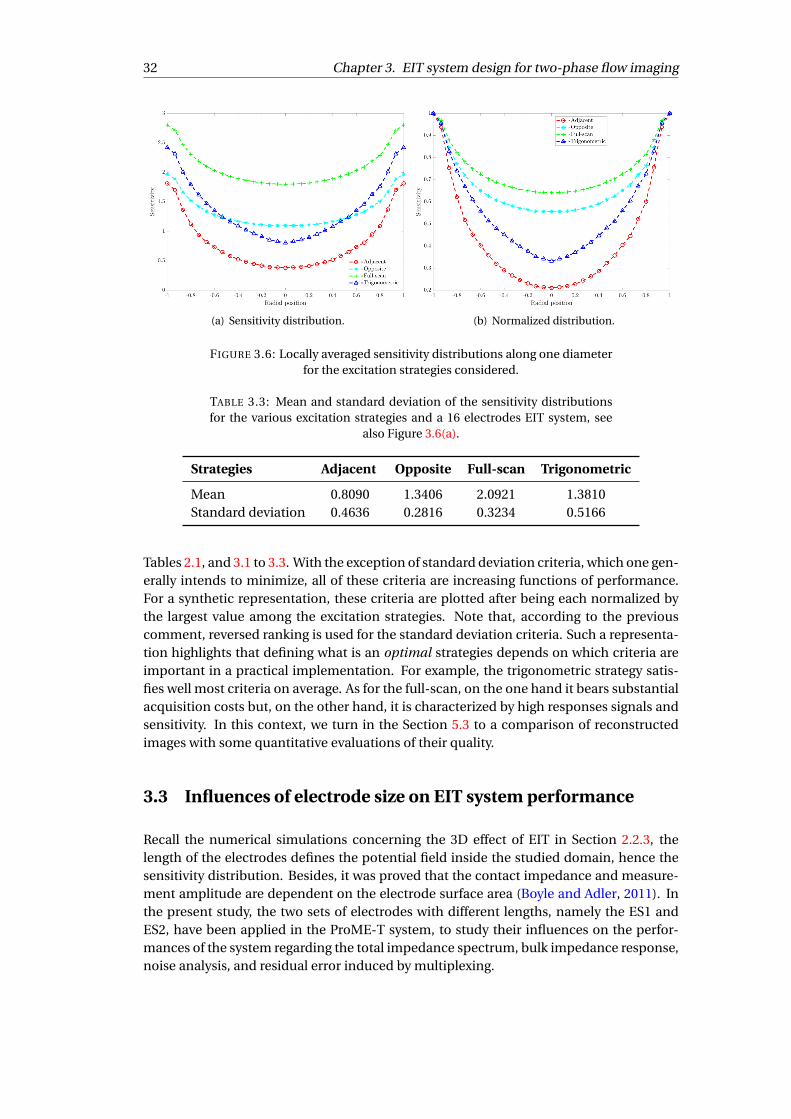
32 Chapter 3. EIT system design for two-phase flow imaging
(a) Sensitivity distribution. (b) Normalized distribution.
FIGURE 3.6: Locally averaged sensitivity distributions along one diameterfor the excitation strategies considered.
TABLE 3.3: Mean and standard deviation of the sensitivity distributionsfor the various excitation strategies and a 16 electrodes EIT system, see
also Figure 3.6(a).
Strategies Adjacent Opposite Full-scan Trigonometric
Mean 0.8090 1.3406 2.0921 1.3810Standard deviation 0.4636 0.2816 0.3234 0.5166
Tables 2.1, and 3.1 to 3.3. With the exception of standard deviation criteria, which one gen-erally intends to minimize, all of these criteria are increasing functions of performance.For a synthetic representation, these criteria are plotted after being each normalized bythe largest value among the excitation strategies. Note that, according to the previouscomment, reversed ranking is used for the standard deviation criteria. Such a representa-tion highlights that defining what is an optimal strategies depends on which criteria areimportant in a practical implementation. For example, the trigonometric strategy satis-fies well most criteria on average. As for the full-scan, on the one hand it bears substantialacquisition costs but, on the other hand, it is characterized by high responses signals andsensitivity. In this context, we turn in the Section 5.3 to a comparison of reconstructedimages with some quantitative evaluations of their quality.
3.3 Influences of electrode size on EIT system performance
Recall the numerical simulations concerning the 3D effect of EIT in Section 2.2.3, thelength of the electrodes defines the potential field inside the studied domain, hence thesensitivity distribution. Besides, it was proved that the contact impedance and measure-ment amplitude are dependent on the electrode surface area (Boyle and Adler, 2011). Inthe present study, the two sets of electrodes with different lengths, namely the ES1 andES2, have been applied in the ProME-T system, to study their influences on the perfor-mances of the system regarding the total impedance spectrum, bulk impedance response,noise analysis, and residual error induced by multiplexing.
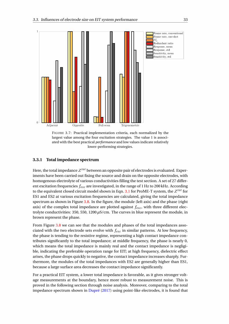
3.3. Influences of electrode size on EIT system performance 33
FIGURE 3.7: Practical implementation criteria, each normalized by thelargest value among the four excitation strategies. The value 1 is associ-ated with the best practical performance and low values indicate relatively
lower-performing strategies.
3.3.1 Total impedance spectrum
Here, the total impedance Z tot between an opposite pair of electrodes is evaluated. Exper-iments have been carried out fixing the source and drain on the opposite electrodes, withhomogenous electrolyte of various conductivities filling the test section. A set of 27 differ-ent excitation frequencies fexc are investigated, in the range of 1 Hz to 200 kHz. Accordingto the equivalent closed circuit model shown in Eqn. 3.1 for ProME-T system, the Z tot forES1 and ES2 at various excitation frequencies are calculated, giving the total impedancespectrum as shown in Figure 3.8. In the figure, the module (left axis) and the phase (rightaxis) of the complex total impedance are plotted against fexc , with three different elec-trolyte conductivities: 350, 550, 1200µS/cm. The curves in blue represent the module, inbrown represent the phase.
From Figure 3.8 we can see that the modules and phases of the total impedances asso-ciated with the two electrode sets evolve with fexc in similar patterns. At low frequency,the phase is tending to the resistive regime, representing a high contact impedance con-tributes significantly to the total impedance; at middle frequency, the phase is nearly 0,which means the total impedance is mainly real and the contact impedance is negligi-ble, indicating the preferable operation range for EIT; at high frequency, dielectric effectarises, the phase drops quickly to negative, the contact impedance increases sharply. Fur-thermore, the modules of the total impedances with ES2 are generally higher than ES1,because a large surface area decreases the contact impedance significantly.
For a practical EIT system, a lower total impedance is favorable, as it gives stronger volt-age measurements at the boundary, hence more robust to measurement noise. This isproved in the following section through noise analysis. Moreover, comparing to the totalimpedance spectrum shown in Dupré (2017) using point-like electrodes, it is found that

34 Chapter 3. EIT system design for two-phase flow imaging
FIGURE 3.8: The module and phase of the total impedance changing withexcitation frequencies, three different electrolyte conductivities are used
for each electrode set.
the middle frequency range extends further to the left (low frequency region) as the elec-trode size increases. In the current thesis study, the excitation frequencies used in ProME-T for measurements of static and dynamic experiments range from 5 kHz to 80 kHz.
3.3.2 Bulk impedance
Calibration is a procedure to compute the bulk impedance by subtracting the correspond-ing electrode-specific contact impedances from the total impedance. Considering Eqn. 3.1and a homogeneous medium in the test section, when the source and drain switch amongthe 16 electrodes, there will be 16 contact impedances Z sour ce or Z dr ai n at the electrodes,and 8 different bulk impedances associated with the angular distances between the sourceand drain. Implementing the full-scan strategy, each excitation pattern gives a linearequation as Eqn. 3.1, forming an array of 120 equations with 24 unknowns, which canbe solved in the least squares sense, the contact impedance at each electrode is obtained,hence the bulk impedance Z . Figure 3.9 shows the bulk impedance of each excitationpattern for both ES1 and ES2 electrodes, applying an excitation frequency of fexc = 50 kHz.The impedances before and after calibration are the total impedance and bulk impedance,respectively. The abscissa represents the index of excitation pattern.
As we can see, the ES1 gives comparable total and bulk impedances, indicating the lowcontact impedance associated with large electrode size. Besides, for both ES1 and ES2the bulk impedances after calibration depend only on the angular separations betweensource and drain, verifying the reliability of the measurements from the present system:the systematic errors can be diminished taking the difference measurements between twoframes, which is a common strategy used in difference image reconstructions.

3.3. Influences of electrode size on EIT system performance 35
FIGURE 3.9: Total and bulk impedances of each excitation pattern in thefull-scan strategy, for two sets of electrodes.
3.3.3 Noise analysis
In a practical EIT system, measurement noise may originate from the system or back-ground environment, including: 1) the higher harmonics of the signal; 2) cross-talks amongchannels; 3) transients induced by multiplexing operation; 4) external noise, such as back-ground noise. During data post-processing, the time domain measurements are trans-formed into frequency domain by FFT, only the amplitudes at excitation frequency areconsidered as the fundamental signals, all the others are discarded as noise. The Signal toNoise Ratio (SNR) is computed as a representation of the noise level:
SNR = 10 · log10
≥Pfundamental freqPPall other freq
¥= 10 · log10
≥ (xFFTi= fexc
)2
Pi 6= fexc
(xFFTi )2
¥, (3.3)
in which xFFTi represents the FFT amplitude at frequency i .
The SNR considers the level of noise relative to the fundamental signal, it is expressedin decibel (dB). To get a reliable estimation of SNR, a high number of samples shouldbe acquired achieving a fine resolution of the FFT spectrum. Excitation voltages at fre-quency fexc = 5 kHz has been applied to a pair of neighboring electrodes (1,2) with ho-mogeneous water of conductivity 750µS/cm filling the test section, 106 samples were ac-quired at 500 kHz acquisition rate in 2 second, the frequency resolution of the FFT spec-trum is thus 0.5 Hz. The voltage measurement across the constant resistor R0 features ahigh amplitude signal, while across electrode pair (9,10) it is extremely low. Their spec-trums associated with ES2 electrodes are plotted as in Figure 3.10. In the plots, the peaksat 5 kHz are the fundamental amplitudes, the rest are noises. The peaks at frequenciesof multiple of fexc scaling with the fundamental amplitudes are higher-order harmonicsinduced by non-linearities in the electronics of the data acquisition system. The baselinenoises, or background noises, are homogeneously distributed at all frequencies, invariantwith fundamental amplitudes.

36 Chapter 3. EIT system design for two-phase flow imaging
(a) High amplitude measurements, ES2. (b) Low amplitude measurements, ES2.
FIGURE 3.10: Spectrums of the high and low amplitude measurementsusing ES2 electrodes, with homogeneous water of conductivity 750µS/cm
in the test section.
FIGURE 3.11: The Signal to Noise Ratio (SNR) of two sets of electrodes.
The corresponding SNR of each measurement channel are computed by Eqn. (3.3) forboth sets of electrodes and plotted in Figure 3.11, the abscissa represents the signal ampli-tude of each channel. As we can see, the SNR are low for both ES1 and ES2, characterizinga low noise level under laboratory environment. Generally, the SNR decreases with signalamplitude, such that the ES2 gives some higher SNR associated with its lower amplitudesignals (on the left). Besides, both ES1 and ES2 give low amplitude measurements in mV,which can be easily distorted by the noise under complex environment.
The SNR and spectrum analysis in frequency domain highlight the origin and level of thenoise, however, they are insufficient to evaluate the noise resistance of the system, as onlythe fundamental signal of FFT is kept in post-processing. The repeatability of the mea-surements is conventionally used to assess the noise robustness of an EIT system. That is,a number of consecutive frames are taken repeatedly under a certain configuration, the

3.3. Influences of electrode size on EIT system performance 37
Relative Error (RE) of each measurement is assessed by
RE =°10 · log10
≥ Pnci=1 V 2
iPnci=1(Vi °Vi )2
¥(3.4)
with Vi the measurement at i th frame, nc the number of repeating frames, Vi the meanvalue of Vi of all frames. Finally, the RE for all the 1920 measurements (` = 16 chan-nels with Ne = 120 excitation patterns) in full-scan strategy could be obtained, their meanvalue RE is taken as the indicator to the repeatability of the measurements, a higher REmeans a better consistency among the repeated frames, hence a higher resistance to noise.
Here, nc = 50 consecutive frames has been acquired at fexc = 50 kHz, the RE of each mea-surement is plotted versus the corresponding signal amplitude for ES1 and ES2 in Fig-ure 3.12. Their mean values RE are 68 dB and 48 dB for ES1 and ES2, respectively. As wecan see, the RE decreases with signal amplitude for both ES1 and ES2, and generally itis lower for ES1 than ES2 at the same signal amplitude, possibly because of the low con-tact impedance associated with ES1. Besides, the RE tends to cluster into a line for eachelectrode set, which may be caused by the propagation of the discretization error of theexcitation signal during FFT.
FIGURE 3.12: Relative errors of all measurements at 50kHz excitation fre-quency for ES1 and ES2.
3.3.4 Residual error analysis
Considering the switch operation performed in multiplexing, it introduces a transientnoise to the measurements associated with the former excitation electrodes, where a cer-tain residual voltage might remain for a short time after switching. Although filtering isapplied to the signal by discarding the out-of-frequency components in the FFT spectrum,significant error may sustain if insufficient data is discarded.
To investigate the residual error induced by multiplexing, the measurements are classifiedinto four categories: i) measurements over the constant resistor R0; ii) measurements over

38 Chapter 3. EIT system design for two-phase flow imaging
the excitation electrodes; iii) measurements at previous excitation electrodes; iv) mea-surements at the other electrodes. The type 3 measurement is of special interest becauseit just experienced a switch operation.
Experiments have been done with fexc = 50 kHz and homogeneous water of conductivity750µS/cm filling the test section. The number Np of periods per excitation pattern is fixedas Np = 10 with Nsp = 20 samples per period, giving 200 data points per excitation patternat each channel. The measured data are then sliced into 10 blocks, one period for eachblock, to which the FFT is performed respectively. Using the fundamental amplitude fromthe 10-th period as reference, the relative error of each period is computed and plotted inFigure 3.13 for both sets of electrodes, for the sake of clarity, one measurement channel isselected to represent each of the four measurement types.
Overall, the measurement errors for the four types of measurements are small (lower than1%), especially for type 1 and 2, the relative errors are well below 0.1%. The type 4 mea-surements have relative large errors due to their low signal amplitudes. Regarding the sizeof the electrodes, mostly ES2 gives lower errors than ES1, as a result of its higher measure-ment amplitudes, also, the electrons in a larger electrode could be emitted more easily.Considering the errors in type 3 measurements, the influence of switch operation can beclearly seen: the relative error of the first period is much higher than the others. While thisresidual error can be diminished simply by discarding the measurement data from thefirst excitation period. Therefore, it is claimed that discarding the measurements over theexcitation electrodes, which is commonly done in many practical EIT systems, is unnec-essary with current hardware design and electrode configurations. In the present thesisstudy, the measurement data from all measurement channels are taken into account.
To sum up, the superiority of the electrodes with large surface area is evidenced, throughinvestigating the total and bulk impedance responses, the measurement amplitudes, therobustness to noise, and the residual error caused by multiplexing. However, increasingthe length of the electrodes means a larger sensing domain, being less sensitive to smalllocal conductivity changes.
3.4 Dual-plane test section design for the PKL facility
This section concerns the design of a dual-plane test section for the PKL facility. For adual-plane test section, the individual plane can either work independently, by which thebubble velocity can be estimated through cross-correlation of the measurements fromthe two plans (Deng et al., 2001), or work collectively, where cross-plane excitations andmeasurements are performed, the sensitivity in the center of the studied domain may beincreased. Here, the former strategy is the primary concern, the optimal distance betweenthe two planes should be carefully selected (Yan et al., 2006). Additionally, some practicalissues have to be considered for the applications in industrial cases, for example, the cur-rent leakages from the electrodes to the nearby grounded pipe, the limitation of workingspace, the extend of sensing domain, and so on.
To start with, the working space of the EIT sensor in the PKL is introduced. The number ofelectrodes is decided considering the compromise between frame rate and quality of im-age reconstructions. After that, the parameters of the electrodes are determined throughrelative error analysis and/or literature reviews, giving the final design of the dual-planetest section.
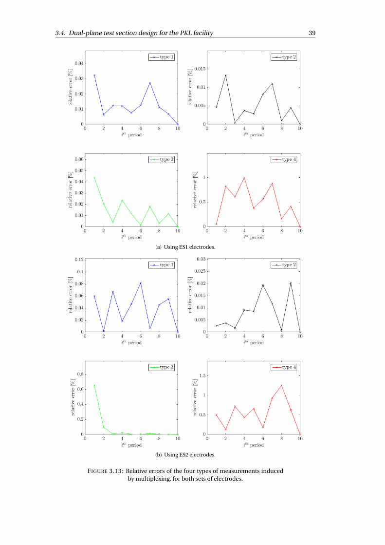
3.4. Dual-plane test section design for the PKL facility 39
(a) Using ES1 electrodes.
(b) Using ES2 electrodes.
FIGURE 3.13: Relative errors of the four types of measurements inducedby multiplexing, for both sets of electrodes.
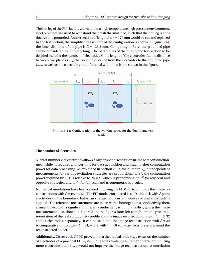
40 Chapter 3. EIT system design for two-phase flow imaging
The hot leg of the PKL facility works under a high temperature high pressure environment,steel pipelines are used to withstand the harsh thermal load, such that the hot leg is con-ductive and grounded. A short section of length LE I T = 170 mm would be cut and replacedby the test section, the simplified 2D scheme of the configuration is shown in Figure 3.14,the inner diameter of the pipe is D = 128.2 mm. Comparing to LE I T , the grounded pipecan be considered as infinitely long. The parameters of the dual-plane test section to bedecided include: the number of electrodes `, the length of the electrodes Le , the distancebetween two planes Ldi s , the isolation distance from the electrodes to the grounded pipeLi so , as well as the electrode circumferential width that is not shown in the figure.
FIGURE 3.14: Configuration of the working space for the dual-plane testsection.
The number of electrodes
A larger number ` of electrodes allows a higher spatial resolution in image reconstruction,meanwhile, it requires a longer time for data acquisition and much higher computationpower for data processing. As explained in Section 2.2.2, the number N i
m of independentmeasurements for various excitation strategies are proportional to `2, the computationpower required by FFT is relative to Ne £`, which is proportional to `2 for adjacent andopposite strategies, and to `3 for full-scan and trigonometric strategies.
Numerical simulations have been carried out using the EIDORS to compare the image re-constructions with `= 16, 32, 64. The EIT model considered is a 2D unit disk with ` pointelectrodes on the boundary. Full-scan strategy with current sources of unit amplitude isapplied. The reference measurements are taken with a homogeneous conductivity, then,a small object with a significant different conductivity is put in the disk, giving the imagemeasurements. As shown in Figure 3.15, the figures from left to right are the pixel rep-resentation of the real conductivity profile and the image reconstructions with `= 16, 32and 64 electrodes, separately. It can be seen that the image reconstruction with ` = 32is comparative to that with ` = 64, while with ` = 16 some artifacts present around thereconstructed object.
Additionally, Gisser et al. (1990) proved that a theoretical limit `max exists on the numberof electrodes of a practical EIT system, due to its finite measurement precision, utilizingmore electrodes than `max would not improve the image reconstruction. A correlation
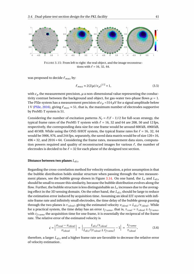
3.4. Dual-plane test section design for the PKL facility 41
FIGURE 3.15: From left to right: the real object, and the image reconstruc-tions with `= 16, 32, 64.
was proposed to decide `max by:
`max º 2(2|µ|/"p )1/2 +1, (3.5)
with "p the measurement precision, µ a non-dimensional value representing the conduc-tivity contrast between the background and object, for gas-water two-phase flows µ = 1.The PXIe system has a measurement precision of "p =314µV for a signal amplitude below1 V (PXIe, 2016), giving `max º 51, that is, the maximum number of electrodes supportiveby ProME-T system is 51.
Considering the number of excitation patterns Ne = `(`° 1)/2 for full-scan strategy, thetypical frame rates of the ProME-T system with ` = 16, 32 and 64 are 208, 50 and 12 fps,respectively, the corresponding data size for one frame would be around 600 kB, 4960 kB,and 40 MB. While using the ONE-SHOT system, the typical frame rates for ` = 16, 32, 64would be 3906, 976, and 244 fps, separately, the saved data matrix would be of size 120£16,496£32, and 2016£64. Considering the frame rates, measurement data sizes, computa-tion powers required and quality of reconstructed images for various `, the number ofelectrodes is decided to be `= 32 for each plane of the designed test section.
Distance between two planes Ldi s
Regarding the cross-correlation method for velocity estimation, a prior assumption is thatthe bubble distribution holds similar structure when passing through the two measure-ment planes, see the bubble group shown in Figure 3.14. On one hand, the Le and Ldi s
should be small to ensure this similarity, because the bubble distribution evolves along theflow. Further, the bubble structure is less distinguishable as Le increases due to the averag-ing effect in the 3D sensing domain. On the other hand, the Ldi s should be large to reducethe estimation error induced by acquisition time. Assuming an ideal EIT system with infi-nite frame rate and infinitely small electrodes, the time delay of the bubble group passingthrough the two planes is øi deal , giving the estimated velocity vi deal = Ldi s/øi deal . Whilefor a practical system, the time delay has an error t f r ame , that is, ør eal = øi deal ± t f r ame ,with t f r ame the acquisition time for one frame, it is essentially the reciprocal of the framerate. The relative error of the estimated velocity is
&=ØØØ
vr eal ° vi deal
vi deal
ØØØ =ØØØ
Ldi s/øi deal
Ldi s/(øi deal ± t f r ame )°1
ØØØ =t f r ame
øi deal, (3.6)
therefore, a larger Ldi s and a higher frame rate are favorable to decrease the relative errorof velocity estimation .

42 Chapter 3. EIT system design for two-phase flow imaging
Compromise should be made ensuring the similarity of bubble distribution and reduc-ing the estimation error induced by acquisition time. For now, there is no mathematicalmodel on this, the Le and Ldi s are commonly decided empirically. Dong et al. (2006) useda pipe of diameter 12.5 cm to study the cross-correlation method for bubble velocity esti-mation, with Ldi s = 10 cm and Le = 1.5 cm, good results were obtained with satisfying ac-curacy. Hao et al. (2017) investigated various distances between two planes of electrodeswith a pipe diameter of 16 cm and electrode length Le = 2 cm, giving an optimal distanceLdi s = 3.5 cm for 3D image reconstruction. Graham and Adler (2007) used Ldi s = 11 cmin a tank of 28 cm diameter and Le = 1 cm, to investigate the influence of electrode place-ment on 3D image reconstructions. Above all, Le = 15 mm and Ldi s = 65 mm are chosenin the current test section design.
Circumferential width of the electrodes
Intensive researches have been done on the influences of electrode size on the perfor-mance of an EIT system. In the topic review of Cheney et al. (1999), it is suggested thatto improve the spatial resolution of EIT, more electrodes should be involved, as well aslarger electrodes that fill as much of the internal circumference as possible. Boyle andAdler (2011) showed that electrodes with larger surface area would provide higher signalamplitude and better image reconstruction. Wtorek et al. (2004) proved that increasingthe electrode size is equivalent to reducing the maximal value of the potential gradientand to introducing the averaging effect of the measurement electrodes. As a result, thevariance of Jacobian’s element value is reduced, which may reduce the ill-posedness of theEIT inverse problem. The numerical simulations concerning the 3D effect and the perfor-mance assessment using the two electrode sets presented in the former sections also ver-ify these results. Therefore, the total circumferential width of the electrodes is decided tooccupy as much of the internal circumference as the manufacture process allows. Finally,the circumferential width of each electrode is 11.5 mm, with a gap between neighboringelectrodes of ª 2.5 mm.
The isolation length Li so is restricted by the total length of the test section, consideringLe +2Li so +Ldi s ∑ 170 mm, it is determined to be Li so = 45 mm given Le and Ldi s . More-over, Darnajou et al. (2018) performed a series of numerical simulations on the currentleakages from the electrodes to the ground pipe with different Le and Li so . The presenteddesign parameters grant a low current leakage concerning the ratio of the leaking powerto the total input power.
The test section design parameters have been further modified before production in co-operation with the mechanical engineer from Framatome GmbH, to meet the practicalmanufacture restrictions. The final design of the dual-plane test section for the PKL facil-ity is presented in Appendix A, see Figure A.1. The electrode design is shown in Figure A.2,the size of the electrodes is 15mm£ 11.5mm£ 1mm for both planes of electrodes, withthe distance between two planes Ldi s = 65 mm and the isolation length Li so = 40.5 mm.

43
Chapter 4
Eigenvalue-based approach using EITraw data
In general, EIT image reconstructions produce smoothing images with low spatial reso-lution compared to the hard-field tomography techniques, like X-ray tomography. Thismakes it difficult to distinguish the phase interface from the reconstructed images. Itera-tive methods yield images of higher resolutions but they usually require high computationpower and are sensitive to measurement noise. In this chapter, an alternative methodol-ogy based on the eigenvalues of the impedance matrix is proposed to estimate the phasefraction inside the studied domain. It circumvents the need to reconstruct images in theextreme non-linear case of two-phase flows, which are characterized by a high resistivitycontrast between phases, while allows to consider a wide range of void fraction.
4.1 Methodology
The proposed methodology is originated from the NtD model introduced in Section 2.2.1,an impedance matrix can be derived as a discrete representation of the NtD map. Con-sidering the closed circuit models of the EIT systems shown in Section 3.1, each excitationpattern has a representative bulk impedance. Implementing the full-scan excitation strat-egy, the impedance array of each frame (with `(`°1)/2 excitation patterns) can be conve-niently arranged into a `£` impedance matrix, which is a symmetric matrix with diagonalentries related to the mutual impedances. In the work of Fang and Cumberbatch (2005),the relation between the void fraction and the eigenvalues of the capacitance matrix ob-tained from ECT data is investigated, it is shown that the multiplicity of the eigenvalues iscorrelated to the degree of symmetry of the flow. Dupré et al. applied the eigenvalue anal-ysis to ECT data for the purpose of flow regime identification as well as the estimation oftwo-phase flow void fraction, the result is promising (Dupré et al., 2017b). In this context,the literature dealing with void fraction estimation from EIT data and through eigenvalueanalysis is scarce. Here, the impedance matrix of EIT is investigated, its eigenvalues areused to devise some metrics of the void fraction.
4.1.1 Mathematical basis
Recall the EIT forward model introduced in Section 2.2.1, the electrostatic potential insidethe domain satisfies the Laplace equation (since æ= 1 in≠\≠i),
¢u = 0, in≠\≠i. (4.1)

44 Chapter 4. Eigenvalue-based approach using EIT raw data
Applying the shunt model Eqn. (4.1) has a unique solution and allows to define a matrixZ , which is the discrete mapping from the boundary current excitations to the boundaryvoltage measurements. The matrix Z is referred to as the impedance matrix and it takesover the role of the NtD operator §æ as its discrete representation. Defining the discreteversion of L2
¶(@≠) as the `-dimensional vector space `¶ = {y = [y1 · · · y`] 2 `,
P`i=1 yi =
0}, one getsZ : `
¶ ! `¶
[I0 I1 · · · I`] 7°! [V0 V1 · · · V`](4.2)
where Vk = u|ek for k = 1, . . . ,` are the boundary measurements of the electric potentialsolution u corresponding to the set of imposed currents Ik considered.
Each element in Z is a bulk impedance corresponding to a certain imposed current andboundary measurement. When the continuous liquid phase is the only conducting phase,given the mixture conductivity æm , the liquid conductivity æl and the liquid volume frac-tion ¥l , the Maxwell-Hewitt relation (Ceccio and George, 1996) reads:
¥l = 1° 1°æm/æl
1+æm/æl, in 2D, ¥l = 1° 1°æm/æl
1+0.5 ·æm/æl, in 3D. (4.3)
This relation yields an approximation of the volume fraction of each phase, as shown inGeorge et al. (2000). The water-gas two-phase flow system conforms this relation, so thatthe measured impedance can be correlated to the void fraction. In the present study, theimpedance matrix contains the impedance of all the possible electrode separations. Inthis framework, the impedance matrix is assumed to be directly correlated to the voidfraction and our objective is to investigate this correlation based on an eigenvalue analysisof numerical and experimental standardized tests.
4.1.2 Impedance matrix and normalization
For each excitation pattern, denoting the source and drain electrodes pair as (i , j ), there isa corresponding bulk impedance Zi , j , which is governed by the conductivity distributionæ(x) in ≠, as well as the selected source and drain electrodes. The impedance betweensource electrode j and drain electrode i is the mutual impedance of Zi , j , so that theysatisfy the reciprocity relation Zi , j = Z j ,i . According to the definition of `
¶ , the diago-nal term Zi ,i is not measured but computed by summing up the corresponding mutualimpedances as Zi ,i = °P
j 6=i Zi , j , which finally yields the `£` square impedance matrixZ = (Zi , j )1∑i , j∑`.
The relative NtD map ¶ = §æ °§0 is commonly used in EIT to retrieve information ofthe probed domain. This amounts to consider the matrix ¢Z = Z ° Z 0, where Z 0 is theimpedance matrix of a homogeneous conductivity distribution for which ≠i = ;. Thematrix ¢Z is referred to as the Differential Impedance Matrix (DIM).
To perform a non-dimensional analysis, a normalization method of the matrix entries Zi , j
is needed to reduce the dependencies on the geometric parameters of the sensor and onthe background conductivity, as well as to enhance the presence of inhomogeneities. Inthis study, the normalization method has been proposed as:
Zi , j =Zi , j °Z 0
i , j
Z 0i , j
for i , j 2 {1, . . . ,`}. (4.4)
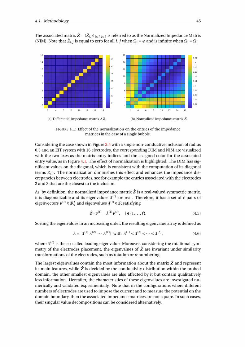
4.1. Methodology 45
The associated matrix Z = (Zi , j )1∑i , j∑` is referred to as the Normalized Impedance Matrix(NIM). Note that Zi , j is equal to zero for all i , j when≠i =; and is infinite when≠i =≠.
(a) Differential impedance matrix ¢Z . (b) Normalized impedance matrix Z .
FIGURE 4.1: Effect of the normalization on the entries of the impedancematrices in the case of a single bubble.
Considering the case shown in Figure 2.5 with a single non-conductive inclusion of radius0.3 and an EIT system with 16 electrodes, the corresponding DIM and NIM are visualizedwith the two axes as the matrix entry indices and the assigned color for the associatedentry value, as in Figure 4.1. The effect of normalization is highlighted: The DIM has sig-nificant values on the diagonal, which is consistent with the computation of its diagonalterms Zi ,i . The normalization diminishes this effect and enhances the impedance dis-crepancies between electrodes, see for example the entries associated with the electrodes2 and 3 that are the closest to the inclusion.
As, by definition, the normalized impedance matrix Z is a real-valued symmetric matrix,it is diagonalizable and its eigenvalues ∏(i ) are real. Therefore, it has a set of ` pairs ofeigenvectors v (i ) 2 `
¶ and eigenvalues ∏(i ) 2 satisfying
Z ·v (i ) =∏(i )v (i ), i 2 {1, . . . ,`}. (4.5)
Sorting the eigenvalues in an increasing order, the resulting eigenvalue array is defined as
∏= [∏(1) ∏(2) · · · ∏(`)] with ∏(1) <∏(2) < ·· · <∏(`), (4.6)
where ∏(`) is the so-called leading eigenvalue. Moreover, considering the rotational sym-metry of the electrodes placement, the eigenvalues of Z are invariant under similaritytransformations of the electrodes, such as rotation or renumbering.
The largest eigenvalues contain the most information about the matrix Z and representits main features, while Z is decided by the conductivity distribution within the probeddomain, the other smallest eigenvalues are also affected by it but contain qualitativelyless information. Hereafter, the characteristics of these eigenvalues are investigated nu-merically and validated experimentally. Note that in the configurations where differentnumbers of electrodes are used to impose the current and to measure the potential on thedomain boundary, then the associated impedance matrices are not square. In such cases,their singular value decompositions can be considered alternatively.
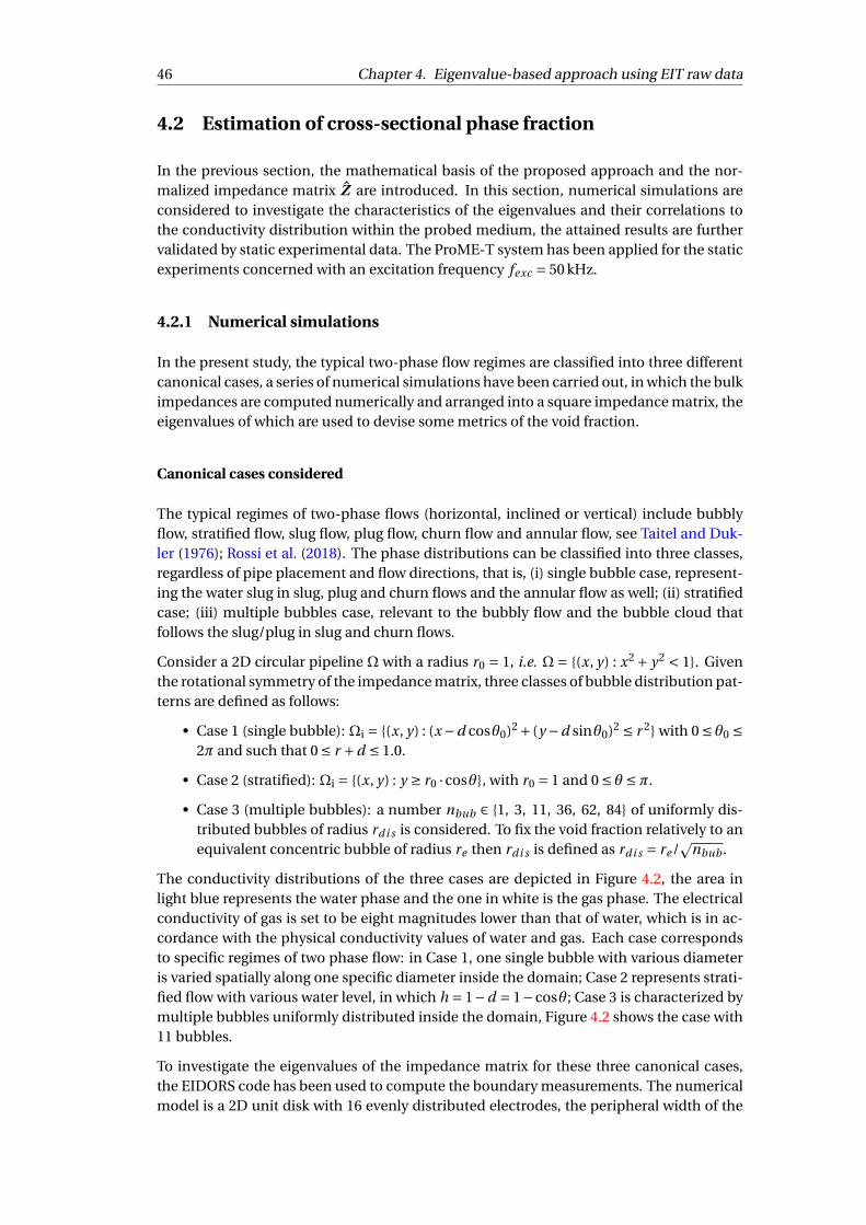
46 Chapter 4. Eigenvalue-based approach using EIT raw data
4.2 Estimation of cross-sectional phase fraction
In the previous section, the mathematical basis of the proposed approach and the nor-malized impedance matrix Z are introduced. In this section, numerical simulations areconsidered to investigate the characteristics of the eigenvalues and their correlations tothe conductivity distribution within the probed medium, the attained results are furthervalidated by static experimental data. The ProME-T system has been applied for the staticexperiments concerned with an excitation frequency fexc = 50 kHz.
4.2.1 Numerical simulations
In the present study, the typical two-phase flow regimes are classified into three differentcanonical cases, a series of numerical simulations have been carried out, in which the bulkimpedances are computed numerically and arranged into a square impedance matrix, theeigenvalues of which are used to devise some metrics of the void fraction.
Canonical cases considered
The typical regimes of two-phase flows (horizontal, inclined or vertical) include bubblyflow, stratified flow, slug flow, plug flow, churn flow and annular flow, see Taitel and Duk-ler (1976); Rossi et al. (2018). The phase distributions can be classified into three classes,regardless of pipe placement and flow directions, that is, (i) single bubble case, represent-ing the water slug in slug, plug and churn flows and the annular flow as well; (ii) stratifiedcase; (iii) multiple bubbles case, relevant to the bubbly flow and the bubble cloud thatfollows the slug/plug in slug and churn flows.
Consider a 2D circular pipeline ≠ with a radius r0 = 1, i.e. ≠ = {(x, y) : x2 + y2 < 1}. Giventhe rotational symmetry of the impedance matrix, three classes of bubble distribution pat-terns are defined as follows:
• Case 1 (single bubble): ≠i = {(x, y) : (x °d cosµ0)2 + (y °d sinµ0)2 ∑ r 2} with 0 ∑ µ0 ∑2º and such that 0 ∑ r +d ∑ 1.0.
• Case 2 (stratified): ≠i = {(x, y) : y ∏ r0 ·cosµ}, with r0 = 1 and 0 ∑ µ ∑º.
• Case 3 (multiple bubbles): a number nbub 2 {1, 3, 11, 36, 62, 84} of uniformly dis-tributed bubbles of radius rdi s is considered. To fix the void fraction relatively to anequivalent concentric bubble of radius re then rdi s is defined as rdi s = re /
pnbub .
The conductivity distributions of the three cases are depicted in Figure 4.2, the area inlight blue represents the water phase and the one in white is the gas phase. The electricalconductivity of gas is set to be eight magnitudes lower than that of water, which is in ac-cordance with the physical conductivity values of water and gas. Each case correspondsto specific regimes of two phase flow: in Case 1, one single bubble with various diameteris varied spatially along one specific diameter inside the domain; Case 2 represents strati-fied flow with various water level, in which h = 1°d = 1°cosµ; Case 3 is characterized bymultiple bubbles uniformly distributed inside the domain, Figure 4.2 shows the case with11 bubbles.
To investigate the eigenvalues of the impedance matrix for these three canonical cases,the EIDORS code has been used to compute the boundary measurements. The numericalmodel is a 2D unit disk with 16 evenly distributed electrodes, the peripheral width of the
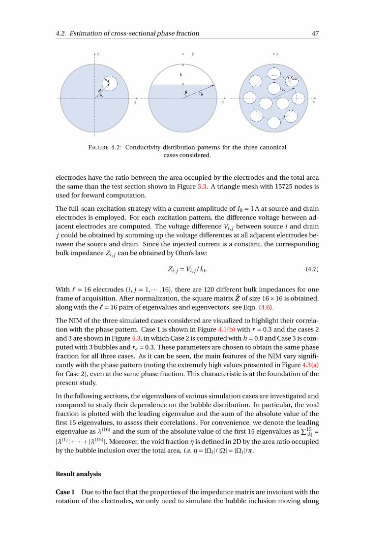
4.2. Estimation of cross-sectional phase fraction 47
FIGURE 4.2: Conductivity distribution patterns for the three canonicalcases considered.
electrodes have the ratio between the area occupied by the electrodes and the total areathe same than the test section shown in Figure 3.3. A triangle mesh with 15725 nodes isused for forward computation.
The full-scan excitation strategy with a current amplitude of I0 = 1 A at source and drainelectrodes is employed. For each excitation pattern, the difference voltage between ad-jacent electrodes are computed. The voltage difference Vi , j between source i and drainj could be obtained by summing up the voltage differences at all adjacent electrodes be-tween the source and drain. Since the injected current is a constant, the correspondingbulk impedance Zi , j can be obtained by Ohm’s law:
Zi , j =Vi , j /I0. (4.7)
With ` = 16 electrodes (i , j = 1, · · · ,16), there are 120 different bulk impedances for oneframe of acquisition. After normalization, the square matrix Z of size 16£16 is obtained,along with the `= 16 pairs of eigenvalues and eigenvectors, see Eqn. (4.6).
The NIM of the three simulated cases considered are visualized to highlight their correla-tion with the phase pattern. Case 1 is shown in Figure 4.1(b) with r = 0.3 and the cases 2and 3 are shown in Figure 4.3, in which Case 2 is computed with h = 0.8 and Case 3 is com-puted with 3 bubbles and re = 0.3. These parameters are chosen to obtain the same phasefraction for all three cases. As it can be seen, the main features of the NIM vary signifi-cantly with the phase pattern (noting the extremely high values presented in Figure 4.3(a)for Case 2), even at the same phase fraction. This characteristic is at the foundation of thepresent study.
In the following sections, the eigenvalues of various simulation cases are investigated andcompared to study their dependence on the bubble distribution. In particular, the voidfraction is plotted with the leading eigenvalue and the sum of the absolute value of thefirst 15 eigenvalues, to assess their correlations. For convenience, we denote the leadingeigenvalue as ∏(16) and the sum of the absolute value of the first 15 eigenvalues as
P15|∏| =
|∏(1)|+· · ·+|∏(15)|. Moreover, the void fraction ¥ is defined in 2D by the area ratio occupiedby the bubble inclusion over the total area, i.e. ¥= |≠i|/|≠| = |≠i|/º.
Result analysis
Case 1 Due to the fact that the properties of the impedance matrix are invariant with therotation of the electrodes, we only need to simulate the bubble inclusion moving along
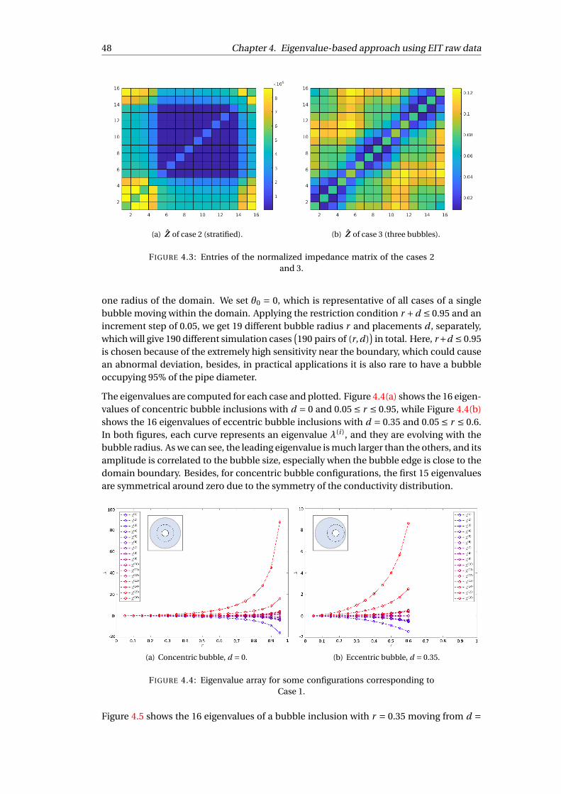
48 Chapter 4. Eigenvalue-based approach using EIT raw data
(a) Z of case 2 (stratified). (b) Z of case 3 (three bubbles).
FIGURE 4.3: Entries of the normalized impedance matrix of the cases 2and 3.
one radius of the domain. We set µ0 = 0, which is representative of all cases of a singlebubble moving within the domain. Applying the restriction condition r +d ∑ 0.95 and anincrement step of 0.05, we get 19 different bubble radius r and placements d , separately,which will give 190 different simulation cases
°190 pairs of (r,d)
¢in total. Here, r+d ∑ 0.95
is chosen because of the extremely high sensitivity near the boundary, which could causean abnormal deviation, besides, in practical applications it is also rare to have a bubbleoccupying 95% of the pipe diameter.
The eigenvalues are computed for each case and plotted. Figure 4.4(a) shows the 16 eigen-values of concentric bubble inclusions with d = 0 and 0.05 ∑ r ∑ 0.95, while Figure 4.4(b)shows the 16 eigenvalues of eccentric bubble inclusions with d = 0.35 and 0.05 ∑ r ∑ 0.6.In both figures, each curve represents an eigenvalue ∏(i ), and they are evolving with thebubble radius. As we can see, the leading eigenvalue is much larger than the others, and itsamplitude is correlated to the bubble size, especially when the bubble edge is close to thedomain boundary. Besides, for concentric bubble configurations, the first 15 eigenvaluesare symmetrical around zero due to the symmetry of the conductivity distribution.
(a) Concentric bubble, d = 0. (b) Eccentric bubble, d = 0.35.
FIGURE 4.4: Eigenvalue array for some configurations corresponding toCase 1.
Figure 4.5 shows the 16 eigenvalues of a bubble inclusion with r = 0.35 moving from d =
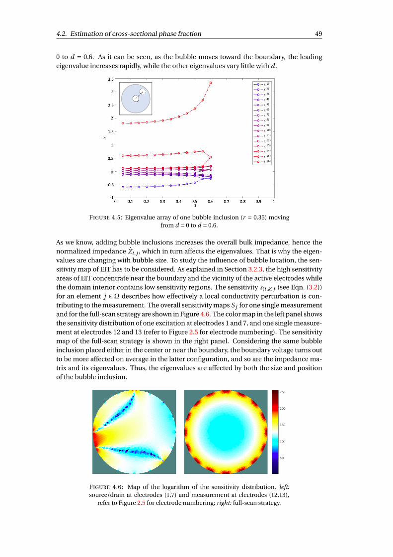
4.2. Estimation of cross-sectional phase fraction 49
0 to d = 0.6. As it can be seen, as the bubble moves toward the boundary, the leadingeigenvalue increases rapidly, while the other eigenvalues vary little with d .
FIGURE 4.5: Eigenvalue array of one bubble inclusion (r = 0.35) movingfrom d = 0 to d = 0.6.
As we know, adding bubble inclusions increases the overall bulk impedance, hence thenormalized impedance Zi , j , which in turn affects the eigenvalues. That is why the eigen-values are changing with bubble size. To study the influence of bubble location, the sen-sitivity map of EIT has to be considered. As explained in Section 3.2.3, the high sensitivityareas of EIT concentrate near the boundary and the vicinity of the active electrodes whilethe domain interior contains low sensitivity regions. The sensitivity s(i ,k) j (see Eqn. (3.2))for an element j 2 ≠ describes how effectively a local conductivity perturbation is con-tributing to the measurement. The overall sensitivity maps S j for one single measurementand for the full-scan strategy are shown in Figure 4.6. The color map in the left panel showsthe sensitivity distribution of one excitation at electrodes 1 and 7, and one single measure-ment at electrodes 12 and 13 (refer to Figure 2.5 for electrode numbering). The sensitivitymap of the full-scan strategy is shown in the right panel. Considering the same bubbleinclusion placed either in the center or near the boundary, the boundary voltage turns outto be more affected on average in the latter configuration, and so are the impedance ma-trix and its eigenvalues. Thus, the eigenvalues are affected by both the size and positionof the bubble inclusion.
FIGURE 4.6: Map of the logarithm of the sensitivity distribution, left:source/drain at electrodes (1,7) and measurement at electrodes (12,13),
refer to Figure 2.5 for electrode numbering; right: full-scan strategy.

50 Chapter 4. Eigenvalue-based approach using EIT raw data
(a) ∏(16) vs. ¥. (b)P15|∏| vs. ¥.
FIGURE 4.7: Eigenvalues vs. void fraction for Case 1.
Figure 4.7 shows the relation between the void fraction and the leading eigenvalue ∏(16)
and the sum of the absolute value of the first 15 eigenvaluesP15
|∏|. For Case 1, the void
fraction satisfies ¥ = ºr 2/ºr 20 = r 2, which is invariant with d . In both figures, each curve
corresponds to a specific value d with varying r , for example, the curve at the right mostrepresents a bubble in the center (d = 0), its radius r increases from 0.05 to 0.95, hence thevoid fraction ranges from 0 to 0.9025. The figures show that both ∏(16) and
P15|∏| increase
with the void fraction and vary with the distance to the center. The void fraction can beestimated by ∏(16) or
P15|∏|, from Figure 4.7 we can estimate the void fraction with an error
less than 10%. Furthermore, the error can be reduced drastically when the position of thebubble is known a priori (distance to the center d).
Case 2 In the stratified configuration, a horizontal liquid-gas interface is considered sincethe impedance matrix is invariant with electrodes rotation. Note that the void fraction ¥
in Case 2 satisfies the relation
¥= (µ° sinµ ·cosµ)/º with µ = arccos(1°h), (4.8)
where h is the height of the gas segment as in Figure 4.2.
The eigenvalue array of Case 2 is plotted in Figure 4.8(a). A linear approximation can befound for the relation between h and the leading eigenvalue, while the data points at highvoid fraction (h > 1.99) are considered to be abnormal and discarded. The other eigenval-ues are not strongly correlated to h. In Figure 4.8(b), ∏(16) is plotted with h, and the curveis fitted linearly with a fitting measure R2 of 0.9905. The deviation between the fitting lineand the data points may originate from the finite number and size of the electrodes andfrom their limited geometrical extent too.
Case 3 In Case 3, a number nbub 2 {1, 3, 11, 36, 62, 84} of bubble inclusions are consid-ered with a radius adjusted to get the same water fraction as an equivalent single concen-tric bubble of radius re . The void fraction of Case 3 is calculated by ¥ = r 2
e , it is restrictedby nbub to avoid contact among bubbles. With nbub = 3 the top limit of void fraction is 0.5,for nbub = 11 it is 0.6, while for other cases it ranges from 0.65 to 0.7. For practical two-phase flows, the intensive bubbly flow rarely reaches a void fraction over 0.5, otherwisethe bubbles would collapse and form bigger bubbles and the flow regime would change.

4.2. Estimation of cross-sectional phase fraction 51
(a) Eigenvalue array vs. h. (b) ∏(16) vs. h and its linear fit.
FIGURE 4.8: Eigenvalue arrays and ∏(16) as a function of h for Case 2.
The eigenvalue ∏(16) is plotted with the void fraction and the bubbles radius in Figure 4.9respectively. In Figure 4.9(a) the right most curve represents the single concentric bubblecase, from right to left the curves correspond to an increasing value of nbub . As we cansee, at the same void fraction the leading eigenvalue ∏(16) is increasing with nbub . Thesame behaviour is also observed in Figure 4.9(b): at the same void fraction, ∏(16) is de-creasing with the bubbles radius. Besides, the smaller the bubbles, the stronger the effecton ∏(16), which is shown by the drop of ∏(16) when rdi s is close to zero. After that point∏(16) decreases smoothly as rdi s increases.
(a) ∏(16) vs. ¥. (b) ∏(16) vs. re /p
nbub .
FIGURE 4.9: Eigenvalues vs. void fraction for Case 3.
For the multiple bubbles case, two parameters have to be known to predict the void frac-tion: the eigenvalues and the number of bubbles within the sensor area. However, it is notpractical to observe the bubble distribution inside a pipe. As mentioned, the eigenvaluesof §æ°§0 can be used to locate the inhomogeneities non-iteratively (Brühl, 2001; Hankeand Brühl, 2003), which will be further discussed in Section 5.1.3. It is a promising methodto be combined with the eigenvalue based approach proposed here, to obtain a reliableand accurate void fraction estimation for two-phase flows.

52 Chapter 4. Eigenvalue-based approach using EIT raw data
4.2.2 Robustness of the proposed approach
The properties of the eigenvalue distribution of the normalized impedance matrix Z areanalyzed in the previous section based on 2D simulations. In the present section, therobustness of this methodology is investigated by studying the case where the data is noisyand when the inclusions are conductive.
Noisy data
In practical EIT systems, the boundary measurements are always polluted by some noise,including background white noise or the cross-talk of electrical devices. Thus, the robust-ness of the eigenvalue analysis to noisy data has to be assessed. The averaging relativeerror RE of the measurements in ProME-T system has been evaluated to be above 48 dB atan excitation frequency of 50 kHz and amplitude of 1 V. Given this RE value then adding anoise of 10 dB to the measurement data from numerical simulations is conservative.
(a) ∏(16) vs. ¥ with error bars. (b)P15|∏| vs. ¥ with error bars.
FIGURE 4.10: Eigenvalue trends obtained with noisy data in Case 1.
The noise is added to the measurement data from both the homogenous and inhomo-geneous configurations. The eigenvalues of Case 1 are computed and compared to theresults without noise. Again, ∏(16) and
P15|∏| are the metrics this study is focusing on, so
they are plotted with error bars as in Figure 4.10. The error ª on ∏(16) is computed asª = |∏(16)
noi s y °∏(16)|/∏(16) where ∏(16) is computed without noise and ∏(16)noi s y is computed
with a 10dB noise. The error onP15
|∏| is computed in the same fashion. As we can see, the
relative error for both ∏(16) andP15
|∏| are very small, the maximum values being 4.3% and2.0% respectively.
Extension to conductive inclusions
Apart from the application in two-phase flow measurements, EIT sensors can also be usedin various industrial processes, which may concern conductive inclusions rather thannon-conductive bubbles. Here, the definition of the conductivity contrast R =æhi g h/ælow
from Seagar et al. (1987) is used to represent the conductivity difference between two

4.2. Estimation of cross-sectional phase fraction 53
phases. For water-gas two-phase flows, R tends to infinity. In the section, some con-figurations with R 2 {100, 10, 5, 2.5, 1.25} are simulated and compared to the results as-sociated with R º1 (i.e. water-gas two-phase flows), to assess the general applicabilityof the proposed methodology.
(a) ∏(16) vs. ¥. (b)P15|∏| vs. ¥.
FIGURE 4.11: ∏(16) andP15
|∏| vs. ¥ for various values of R in Case 1.
All three cases are simulated in 2D when varying R and the results for the cases 1 and2 are plotted in Figures 4.11 to 4.12. In Figure 4.11(a), the eigenvalue ∏(16) for the singleconcentric bubble case is plotted with ¥ and each curve represents different values of R.As we can see, the trends of ∏(16) changing with ¥ are similar for different values of R,while the amplitude are increasing globally with R. Also, as R increases to large values,∏(16) increases less and less, especially after R = 100, i.e. there exists a threshold effect.The same conclusions are obtained for
P15|∏|, see Figure 4.11(b).
(a) ∏(16) vs. h, all cases. (b) ∏(16) vs. h, excluding R =1.
FIGURE 4.12: ∏(16) vs. h in Case 2.
For the stratified case, the same results can be obtained, while the contrast R has a muchstronger effect on the eigenvalues, especially for large values. As shown in Figure 4.12,∏(16) is 5 to 6 magnitudes higher for R =1 than for the other cases, so that ∏(16) vs. h isplotted in Figure 4.12(b) excluding the case R =1. Nevertheless, a linear correlation canbe found between ∏(16) and h for varying R.
Lastly, the results for the multiple bubbles case have been found to be similar to the sin-gle bubble case. The applicability of the eigenvalue analysis to conductive inclusions is

54 Chapter 4. Eigenvalue-based approach using EIT raw data
therefore emphasized but the conductivity contrast R between phases is an importantinformation to be known beforehand.
4.2.3 Validation by static experiments
In this section, the proposed methodology, which has been devised based on numericalsimulations, is validated experimentally. Static experiments were performed in LTHC witha pipe containing still water, for a number of configurations corresponding to the three in-clusion patterns considered previously. The motivations for performing such static exper-iments are as follows: (i) they are easily implementable using standard laboratory equip-ment and allow to control the phase distribution accurately, which is crucial to validatethe proposed approach, (ii) EIT measurements can be performed at a high frame rate (ofthe order of 800 fps for the system considered), which allows to treat a dynamic flow as ifit were quasi-static on each frame.
These static experiments were carried out with the ProME-T system using the test sec-tion shown in Figure 3.3. The system uses voltages of ±1 V as excitation signals, whichis different from the current excitation considered in the numerical simulations but weconsider the two settings as being equivalent. For the single bubble and multiple bubblescases, different diameters and numbers of rods were placed into the water to emulate bub-bles, giving various void fractions. Considering the complete model, the bulk impedancefor both homogeneous and inhomogeneous configurations can be obtained excluding theelectrode specific contact impedance from the total impedance, as shown in Section 3.3.2,giving the corresponding normalized impedance matrix Z .
Result comparison
Numerical simulations in 2D can be considered as being equivalent to configurations withinfinite long electrodes and inclusions, while in practical 3D implementations, the elec-trodes and the inclusions have finite extents. Therefore, it is more relevant to compare theresults from a practical EIT system with 3D simulations. As a consequence, we considerhere a 3D cylindrical model implemented in EIDORS, as shown in Figure 4.13. The radiusof the numerical model is 1 while all other parameters are normalized from the prototypeEIT system so that the length of the model is 7.5, the electrodes have a width of 0.125 anda length of 4.25. A fine tetrahedral mesh with 54308 nodes is generated on the 3D simu-lation model. The bubble inclusion is emulated by a non-conductive rod of the height ofthe model.
As of the static experiments, a series of configurations were investigated to obtain datafor all of the three patterns considered. For Case 1, a single non-conductive rod withdifferent diameters was placed in the test section at different distances to the center:the diameter of the rod ranges from 10 mm to 70 mm, the distance to the center beingd 2 {0, 12, 24} mm, corresponding to d 2 {0, 0.3r0, 0.6r0} in the 3D simulations. For Case2, the test section was placed horizontally with different water levels. In Case 3, differentexperiments with three rods placed symmetrically were carried out, the diameter of therods ranges from 10 mm to 40 mm. The normalized impedance matrix and its eigenvalueswere computed for each case. The evolutions of the eigenvalue ∏(16) with the void fractionare shown along with 3D simulation results in Figure 4.14 for the cases 1 and 3, and inFigure 4.15 for Case 2.

4.2. Estimation of cross-sectional phase fraction 55
FIGURE 4.13: 3D simulation model to compare with the static experi-ments, non-conductive rods with the same height of the model would be
used to emulate the bubble inclusion.
(a) Case 1. (b) Case 3.
FIGURE 4.14: Comparison between 3D simulations and experimentalstatic experiments for the cases 1 and 3: eigenvalue ∏(16) as a function of
the void fraction ¥.
For the cases 1 and 3, the trends of the eigenvalue ∏(16) for the static experiments agreewell with the 3D simulations, which validates the proposed methodology. Deviations oflow relative amplitude can be observed, which may be due to the following facts: (i) thesimulation model is non-dimensional with normalized size and conductivity; (ii) the stim-ulation signal is a constant current in the simulations while it is a constant voltage in theexperiments.
For Case 2, the trends of the eigenvalue ∏(16) with the thickness h of the gas layer, see (4.8),for the experiments and the 3D numerical simulations are very different, as seen in Fig-ure 4.15(a), especially at small h. The magnitudes in the experiments are also significantlylower than in the simulations. These discrepancies may come from: (i) the surface tensionof water causes a rise at the interface between the plastic pipe and the water, especially atlow h; (ii) a conductive water film may be present on the uncovered part of the pipe sur-face, while in the simulation there is no such film. Moreover, the magnitude of the eigen-value ∏(16) is remarkably high for all values of h compared to the other phase distributionpatterns (at the same void fraction), as shown in Figure 4.15(b). Lastly, the electrodes thatare immersed in water can be directly revealed by the distribution of the entries of thenormalized impedance matrix, as seen in Figure 4.3(a), which could therefore be used asan indicator of the water level.

56 Chapter 4. Eigenvalue-based approach using EIT raw data
(a) ∏(16) vs. h. (b) ∏(16) vs. ¥ for low values of h.
FIGURE 4.15: Comparison between 3D simulations and experimentalstatic experiments for Case 2.
To sum up, the impedance data from EIT sensor and its relation to the void fraction of two-phase flows is investigated numerically and experimentally for a cylindrical pipe config-uration. The boundary measurements at discrete electrodes lead to one bulk impedancematrix for each excitation pattern. A normalization of the impedance matrix is consideredto extract information from the data and reduce the influences of factors other than thebubble inclusion distribution, such as the diameter of the sensor, the background mediumconductivity or the stimulation signal.
Numerical simulations are carried out for three different canonical cases that cover a di-versity of bubble distribution patterns for two-phase flows. Synthetic boundary measure-ments are computed to obtain normalized impedance matrices, the eigenvalues of whichare investigated in the different configurations considered. The robustness of the pro-posed approach to noisy data is assessed by adding 10 dB of noise to the measurementdata and the presented results highlight some satisfying performances. Moreover, thismethodology can be extended to case of conductive inclusions.
From the numerical simulations, it is found that the leading eigenvalue ∏(16) and the sumof eigenvalues
P15|∏| = |∏(1)| + · · · + |∏(15)| are strongly correlated to the void fraction for all
of the cases considered: (i) in the single bubble case (Case 1), the simulation results areencapsulated by the curves of ∏(16) and
P15|∏| vs. ¥ excluding the data point at ¥ > 0.9025.
The void fraction can be estimated byP15
|∏| with an error of 10% regardless of the bubble
position; (ii) in the stratified case (Case 2), a linear correlation is found between ∏(16) andh with a fitting measure R2 = 0.9905; (iii) in the multiple bubbles case (Case 3), the relationbetween the void fraction and the eigenvalues are strongly dependent on the number nbub
of inclusions and an accurate estimation of the void fraction requires the knowledge ofboth ∏(16), or
P15|∏|, and nbub .
Static experiments corresponding to the three cases considered are carried out and theeigenvalues of the NIM from experimental data are compared with 3D simulations. Thetrends for the eigenvalue ∏(16) with ¥ agree well for the cases 1 and 3, although there aresmall deviations in terms of the magnitudes; for Case 2 there is a large discrepancy be-tween the static experiments and the simulations, while ∏(16) is remarkably high at all hcompared to other phase distribution patterns at the same phase fraction.

57
Chapter 5
Image reconstruction of highlycontrasted profiles
The EIT inverse problem can be described as seeking the unknown admittivity distribu-tion from the knowledge of boundary excitation and measurement. Theoretically, all pos-sible boundary measurements determine the internal model parameters uniquely (Som-ersalo et al., 1992), while in practice the number of boundary measurements is limitedby the finite number of electrodes and excitation patterns, yet the measurements are de-graded by measurement error and noise. Therefore, the solution to the EIT inverse prob-lem is usually a discretized conductivity profile with piece-wise constant values.
The EIT inverse problem is challenging because: i) it is a non-linear problem, the electricalcurrent spreads out in the sensing domain in all directions, even out of the sensor plan; ii)it is severely ill-posed, the boundary measurement is much more sensitive to conductiv-ity change near the boundary than in the center. Intensive researches have been carriedout on the EIT image reconstruction algorithms. In this chapter, the conventional andnon-conventional reconstruction algorithms or methods for the EIT are reviewed, someof them are implemented using numerical simulation data. The reconstruction methodsfeasible for two-phase flow imaging are decided, with which benchmark reconstructionsare made for several static experiments. In addition, the quality of the reconstructed im-ages associated with various excitation strategies are compared quantitively using bothsimulation and static experimental data.
5.1 Review of image reconstruction methods
The approaches to the EIT inverse problem is straightforward: linearize the non-linearproblem, reduce the ill-posedness through regularization, and solve a sequence of lin-earized problem iteratively to reconstruct large conductivity contrasts or complex geome-tries. Various iterative and non-iterative algorithms have been thoroughly investigatedand compared in the context of high contrast imaging in chemical engineering or pro-cess tomography, see e.g. Kim et al. (2001); Kotze et al. (2019), and comprehensive reviewspresented in Lionheart (2004), Polydorides (2002) and Borcea (2002).
Non-iterative algorithms are commonly based on the linear assumption: the conductivityprofile is close to a constant. Typical approaches include the sensitivity back-projection(Santosa and Vogelius, 1990; Kotre, 1994; Barber and Brown, 1984), one-step Newton method(Cheney et al., 1990; Fuks et al., 1991), and so on. Iterative methods solve the reconstruc-tion problem minimizing the cost functions in the least-squares sense, such as the mod-ified Newtom-Raphson method (Yorkey et al., 1987) and variational method (Kohn and

58 Chapter 5. Image reconstruction of highly contrasted profiles
McKenney, 1990), the essence is solving a sequence of regularized linear problem and up-dating the conductivity approximation iteratively.
The iteration method may stop at a local minimum without noticing, Breckon (1990)proved that the minimum of the cost function is not unique, it lies in a deep-sided narrowvalley with a very flat floor where the lowest value is hard to find. Also, it is computationallyexpensive solving the direct problem in every iteration. Therefore, non-iterative meth-ods solving the nonlinear inverse problem directly have been proposed, e.g. factorizationmethod (Hanke and Brühl, 2003), topological sensitivity analysis (Bonnet, 2009; Bonnetand Cakoni, 2019), level set method (Chung et al., 2005), and D-bar method (Isaacsonet al., 2004). These methods either only retrieve partial information of the conductivityprofile, for example the position or shape of the inclusion, or require to choose the hyper-parameter subjectively or empirically, since there is rare mathematical model availableon this aspect. Until now, they are mainly investigated theoretically, further studies areneeded implementing with practical EIT data. A comprehensive and in-depth introduc-tion to nonlinear inverse problems with practical applications in Sparse X-ray and EITimaging can be found in Mueller and Siltanen (2012).
5.1.1 Back-projection
Back-projection is a fast reconstruction method widely used in hard-field imaging, suchas the FBP method for X-ray imaging. The idea is to back-project the measured data ontothe probed domain, that is, assigning the measured data to the elements on the trajectoryline connecting the emitter and receiver, an image is formed summating the measurementdata of all projections. For EIT inverse problem, modifications should be made to the con-ventional back-projection, since the trajectory line of electrical current is not straight. Bar-ber and Brown (1984) considered the equipotential line as the current ‘trajectory’ to applyback-projection. Kotre (1994) proposed a sensitivity weighted back-projection approach,the normalized transpose of the Jacobian matrix is applied to the voltage difference data.Typically, a smooth image is obtained from back-projection method. It was widely used inthe process tomography, while shows few advantage than the Tikhonov regularization for-mula with one-step Newton method, which will be introduced in the following sections.
5.1.2 Least-squares methods
The least-squares methods estimate the conductivity profile by minimizing a cost func-tion, or objective function as:
æid = arg minæ©(æ), with©(æ) = 1
2kU (æ)°V k2, (5.1)
where V is a vector of discrete boundary measurements associated with an objective (dis-crete) conductivity distribution to be reconstructed, while U (æ) is a vector of simulatedboundary measurements associated with a trial conductivity field æ, k ·k2 is the standard2-norm on vectors. The minimizer æid gives the reconstructed profile.
Differentiating©with respect to æ, we have:
©0 =U 0(æ)T (U (æ)°V ), (5.2)
in which the term U 0(æ) is essentially the Jacobian matrix J .
5.1. Review of image reconstruction methods 59
Eqn. (5.2) is still nonlinear with æ, thus, a Taylor series expansion at an arbitrary point æk
is taken neglecting the high order terms, giving:
©0(æk +±æk) º©0(æk)+©00(æk)±æk, (5.3)
where©00 is the so-called Hessian matrix, it is given by:
©00 = J T J +U 00(æ)T £I ≠ [U (æ)°V ]
§, (5.4)
with ≠ the Kronecker matrix product (Brewer, 1978), I the identity matrix. The term U 00 isthe second order derivative of U , it is difficult to calculate explicitly, while [U (æ)°V ] be-comes negligible as the minimum is approached, giving the approximate Hessian matrixas:
©00 º J T J . (5.5)
Minimizing the function in Eqn. (5.1) means seeking a step ±æk for which©0(æk+±æk) º 0,by substituting Eqn. (5.2) and (5.5) into Eqn. (5.3), we have:
±æk =°(J T J )°1 J T [V °U (æk)], (5.6)
which is an iteration step to find æid for the nonlinear inverse problem through the well-known Gauss-Newton iteration. From an initial point, usually a homogeneous conductiv-ity profile is taken, the conductivity approximation is updated by ±æk at each step, that is,æk+1 =æk+±æk, withæk andæk+1 the conductivity estimation at step k and k+1, separately.The procedure continues until the convergence criteria is reached, the approximation atthe final step corresponds to æid. Nevertheless, this procedure can be stopped at the firststep, giving the so called one-step Gauss-Newton method.
Unfortunately, in the presence of measurement error the Gauss-Newton iteration does notwork well: the term [V °U (æk)] may be below the measurement error, leading to an unde-sired conductivity approximation. Also, the Hessian matrix J T J is highly ill-conditioned,which makes its inverse very inaccurate and sensitive to measurement errors.
Thus, regularization techniques are applied to improve the conditioning of the objectivefunction, that is, a penalty regularization term Q(æ) is introduced into©, the least-squaresproblem is now to seek æid minimizing:
©= 12kU (æ)°V k2 +ÆQ(æ), (5.7)
where Æ 2 is the non-negative regularization hyperparameter to be chosen from caseto case, while Q(æ) can have various forms, corresponding to different types of regular-izations. In Eqn. (5.7), the first term represents the fidelity to the measurement data, thesecond term incorporates certain a priori information into the cost function, Æ acts as aweighting coefficient to control the tradeoff between the two terms. The regularizationterm improves the stability of the reconstruction algorithm, while it incorporates a prioriinformation which may be unrepresentative of the real conductivity profile.
The hyperparameter Æ is a critical parameter to choose in regularized image reconstruc-tions, it controls the weighting of the penalty term in the objective function. A large Æ
smoothens the reconstructed image, a small Æ gives more weight to data misfit and offersincreased resolution. However, if it is set too small, the data lying below the noise thresh-old dominates the inverse matrix, the resulting image represents measurement noise in-stead of conductivity distribution.

60 Chapter 5. Image reconstruction of highly contrasted profiles
There are several ways to decide the optimal hyperparameter depending on whether thenoise covariance of the measurement is known or not (Vauhkonen, 1997), e.g. discretePicard condition method, Moore-Penrose method, and L-curve method. Amongst, the L-curve method is the most widely applied approach, although it gives case specific optimalvalues associated with the conductivity profiles concerned. It is noted that Graham andAdler (2006) used the so-called ‘blur ratio’ as a representation to image resolution and pro-posed the BestRes method to obtain the optimal hyperparameter that gives the minimumblur ratio. The advantage is that the optimal Æ is universal to all conductivity profiles andnoise levels.
Tikhonov type regularization
A typical choice of Q(æ) is a quadratic function, substituting into Eqn. (5.7), we have thegeneralized Tikhonov type regularization for EIT inverse problem:
æid = arg minæ©(æ), with©(æ) = 1
2kU (æ)°V k2 +ÆkL(æ°æref)k2, (5.8)
withæref a reference conductivity profile, L the regularization matrix which is the approx-imation to some partial differential operators.
The L2-norm of Tikhonov type regularization guarantees its non-negativity, so that theresulting functional is differentiable, leading to a well-posed minimization problem (theinversion is stabilized). An approximate solution for Eqn. (5.8) is:
±æk =°(J T J +ÆLT L)°1°J T±V k +ÆLT L(æref °æk)¢, (5.9)
with ±V k =V °U (æk). Applying the Gauss-Newton iteration, the regularized inverse prob-lem is solved using the same procedure as the non-regularized one.
To understand how regularization ameliorates the ill-posed problem, the condition num-bers ∑ of the inverse terms in Eqn. (5.6) and (5.9), that is, J T J and (J T J +ÆLT L), are com-pared. The condition number ∑ can be used as an indicator of the ill-posedness of a prob-lem, the larger the condition number, the more ill-posed the inverse problem. Here, ∑ isdefined as ∑(A) =∏n(A)/∏1(A), with ∏n(A) and ∏1(A) the maximum and minimum eigen-values of a matrix A, a larger ∑ means a higher ill-conditioning. Taking a simple case withL = I , the condition numbers with and without regularization are:
∑= ∏n(J T J )∏1(J T J )
, without regularization,
∑= ∏n(J T J )+Æ∏1(J T J )+Æ
, with regularization.
(5.10)
The ill-conditioned matrix J T J has a sufficiently small eigenvalue ∏1(J T J ), the ∑ in regu-
larized case is approximated as ∑º ∏n (J T J )Æ +1, implying a well-conditioned problem with
a large Æ.
Various regularization matrices L incorporating different a priori information can be used,e.g. the identity matrix I , or the matrices corresponding to the first and second orderdifference operators. For example, using the penalty form kæk2 gives good result if theconductivity distribution is known to be bounded and fluctuating, kæ0k2 fits a continuousconductivity profile, while kæ00k2 gives a smooth solution (Hua et al., 1988). Also, there are

5.1. Review of image reconstruction methods 61
regularizations exploiting the information from the sensitivity matrix J , i.e. the standardTikhonov regularization.
In standard Tikhonov regularization, the regularization matrix is scaled with the sensitivityof each element, giving L = diag(J T J )p , with 06 p 6 1 an exponent coefficient. The valueof p can be chosen arbitrarily, it is a compromise between pushing noise to the boundary(for p = 0) or to the centre (for p = 1). It becomes the Zeroth-order regularization with L =I when p = 0, and gives the Newton’s One-Step Error Reconstructor (NOSER) algorithm(Cheney et al., 1990) with p = 1.
The NOSER method is widely used in practical EIT image reconstructions for flow mon-itoring and clinical imaging, benefiting from its low computation cost and robustness tonoise. It performs only one step of iteration with an updating step:
¢æ=°°
J T J +Æ ·diag(J T J )¢°1 J T¢V , (5.11)
where ¢V = Vi °Vh is the differences between the image measurements Vi associatedwith the conductivity distribution to be reconstructed and the reference measurementsVh associated with the reference conductivity distribution, which is usually taken as ahomogeneous conductivity. The inverse matrix, being (J T J +Æ ·diag(J T J ))°1 J T , can bepre-calculated and saved, allowing a fast image reconstruction for online display.
Total variation regularization
Another type of regularization term Q(æ), i.e. the Total Variation (TV) regularization, takesthe L1-norm formula. The resulting TV regularized least-squares problem has the form:
æid = arg minæ©(æ), with©(æ) = 1
2kU (æ)°V k2 +ÆkLæk1. (5.12)
In continuum form, the TV of a conductivity profile is defined as:
T V =Z
≠|ræ|d≠, (5.13)
with ≠ the sensing domain. Considering the discretization with pixel-wise constant con-ductivity, ræ is non-null only on the edges between elements, where the conductivitypresents a step change from one element to the other, giving the discretized TV matricesas:
T V =X
ikLiæk1, (5.14)
where L is a sparse matrix with one row per each edge in the mesh, and every row Li
has two nonzero elements in column m and n, which are the indices of the two elementssharing the same edge, for example,
Li = [0, · · · ,0,1, · · · ,0,°1, · · · ,0]. (5.15)
The L1-norm guarantees a positive penalty term, however, it leads to the minimization ofa non-differentiable function |ræ|, which cannot be solved efficiently with conventionalGauss-Newton method. In the research of Borsic et al. (2009), the Primal Dual-InteriorPoint Methods (PDIPM) is proposed to solve the TV regularized functional numerically.

62 Chapter 5. Image reconstruction of highly contrasted profiles
The TV regularization rules out wild fluctuations in conductivity while preserving discon-tinuities in the reconstructed profile, its ability in reconstructing sharp conductivity con-trasts gives clear benefits to two-phase flow imaging: it may yield a better phase segmen-tation. It is noting that the TV regularization is normally applied in iterative reconstruc-tions, because it converges much slower than quadratic regularizations, stopping at thefirst iteration step would not give valuable information about the conductivity profile.
Some other regularization forms are available incorporating various a priori information,e.g. the information from magnetic resonance imaging, the noise level of the measure-ment system. A good review can be found in Vauhkonen (1997).
Probabilistic regularization
The Tikhonov and TV regularizations are essentially deterministic regularizations thatincorporate a priori knowledge or assumption on the conductivity profile to be recon-structed, which may be unrealistic in many cases. On the contrary, the probabilistic reg-ularization treats the conductivity distribution as random variables with probability dis-tributions. Considering the Bayes’ theorem relating conditional probabilities of randomvariables:
P (x|b) = P (b|x)P (x)P (b)
, (5.16)
the most likely x is obtained through maximizing P (x|b), giving the so-called MaximumA Posteriori (MAP) approach (Holder, 2004). The Gaussian high pass filter regularizationproposed in Adler and Guardo (1996) is a good example of the MAP approach using knowl-edge of the noise variance of the measurement and the covariance of the conductivitydistribution.
The GREIT method
A specialized reconstruction method, namely the Graz consensus Reconstruction algo-rithm for EIT (GREIT), has been proposed based on the consensus of a large and repre-sentative group of experts in EIT algorithm design and clinical applications for pulmonarymonitoring (Adler et al., 2009). It is a linear reconstruction method producing conductiv-ity difference images in 2D or 3D (Grychtol et al., 2016). The reconstructed differenceimage ¢æ is calculated from an inverse matrix R and the difference data ¢V =Vi °Vh by:
¢æ= R ¢V . (5.17)
Conventionally, R is computed from the ill-conditioned EIT inverse problem with lin-earization and regularization, while in GREIT the best inverse matrix R is obtained throughoptimizing several performance metrics, namely the amplitude response, position error,ringing artifacts, shape deformation, resolution, and noise figure, associated with a num-ber of small ‘training’ targets following some specific distribution patterns inside the for-ward model.
Similar to the NOSER algorithm, the best inverse matrix R of GREIT can be pre-calculatedand saved for online image reconstruction. Also, the GREIT is designed favoring the clin-ical applications, which is analog to two-phase flows in terms of high conductivity con-trasts and sharp interfaces between the objects and the background. Therefore, it is ofinterest to test the GREIT method in two-phase flow imaging.

5.1. Review of image reconstruction methods 63
5.1.3 Factorization method
Unlike the conventional image reconstruction methods giving the conductivity approxi-mations within the studied domain, the Factorization Method (FM) only allows a binarytest to the points inside the domain, checking whether they are inside the object(s) or not.The method is originated from a far-field inverse scattering theory proposed in the funda-mental research by Kirsch (1998), the main idea is to construct a test function, the value ofwhich shows a singularity peak at a test point inside the object, while a low value outside.The schematic is as shown in Figure 5.1 with four electrodes on the boundary, a virtualtesting grid is put overlaying the studied domain ≠, the value of the test function at eachtest point z is calculated, which would be extremely high for z 2≠i and low for z 2≠\≠i .A binary image can be reconstructed from the FM.
FIGURE 5.1: Schematic of the factorization method with four electrodeson the boundary. The test function gives significant value for a test point
z inside the object≠i .
Defining the test function
The Green’s function is used to construct the test function in Bellis et al. (2012). For a lin-ear differential operator H defined on a domain with specified initial or boundary condi-tions, its Green’s function G(x, s) is defined as the solution of H G(x, s) = ±(s ° x), where ±is Dirac’s delta function, it equals to zero everywhere except for s = x.
Considering the Green’s function for EIT forward problem in the infinite two-dimensionalreal coordinate space 2:
æ¢xG(x, z) = ±(z °x), in 2, (5.18)
while in a closed and connected domain≠with Neumann boundary conditions, we have:
æ¢xG≠(x, z) = ±(z °x), in≠, (5.19)
ærxG≠(x, z) ·n = 0 on @≠, andZ
@≠G≠(x, z)dS = 0. (5.20)
Then, a function N (·, z) =G≠(·, z)°G(·, z) is introduced, so that
æ¢x N (x, z) = 0, in≠, (5.21)

64 Chapter 5. Image reconstruction of highly contrasted profiles
ærx N (x, z) ·n =°ærxG(x, z) ·n, on @≠. (5.22)
The function G(·, z) can be obtained analytically and explicitly, while N (·, z) can be solvednumerically. Specifically for the unit disc case considered in the present study, N (·, z) canalso be solved analytically. Therefore, we have the function G≠(·, z) = N (·, z)+G(·, z), whichis harmonic in ≠ \≠i . The test function is defined as Tz = d ·rG≠(·, z), with d a givenarbitrary unit vector.
Some other researchers (Brühl and Hanke, 2000; Brühl, 2001) defined the test function byintroducing the dipole function:
Dz (x) = 1!n
(z °x) ·d|z °x|n , x 6= z, (5.23)
located in z with an arbitrary unit vector d 2 d°1 = {x 2 d , |x | = 1}, and !n the surfacemeasure of the unit sphere in n . Dz corresponds to the electrostatic potential createdby a dipole source at position z pointing to the direction d . It is then augmented by aharmonic function vz in≠with Neumann data as:
@vz
@n=°@Dz
@n, on @≠, (5.24)
with n the unit outward normal vector on the boundary @≠. The test function is definedas:
Tz = Dz + vz , (5.25)
which is harmonic in ≠ \≠i with vanishing flux @Tz /@n on @≠. Essentially, the test func-tions defined from the dipole function and from the Green’s function are equivalent.
Hanke and Brühl (2003) proved that,
z 2≠i if and only if tz = Tz |@≠ 2 R f (§æ°§0)1/2, (5.26)
with tz the trace of the test function Tz , R f representing the range, and (§æ °§0) therelative NtD map defined in Section 2.2.1.
For the unit disc case, tz can be computed analytically by the explicit expression:
tz =1º
(z °x) ·d|z °x|2 , (5.27)
with x the measurement points on @≠.
Numerical implementation
Picard criterion. In numerical implementation, the range R f (§æ°§0)1/2 in the crite-rion (5.26) is difficult to compute explicitly, the Picard criterion is applied considering theeigenvalues ∏k and eigenvectors vk of (§æ°§0). For the cavity problem, the eigenvalues∏k (sorting in descending order) of (§æ°§0) exhibit exponential decay, so do the squarednorms of the eigen-components htz , vki2. Their average decay parameters are determinedseparately through:
log∏k º c +k log q, k = 1, · · · ,m0,
loghtz , vki2 º ∞z +k logΩz , k = 1, · · · ,m0,(5.28)

5.1. Review of image reconstruction methods 65
with c and ∞z some constant numbers, m0 the number of eigenvalues and eigenvectorsconsidered in the implementation, it is usually small due to the error in approximatingR f (§æ°§0)1/2 and the presence of noise in measurement data. The criterion (5.26) thenbecomes:
z 2≠i if and only if Ωz < q. (5.29)
Computing ∏k and vk . In continuum form, considering the boundary excitation as atrigonometric function f and the difference measurement as ¢V = Vi °Vh , with Vi theboundary measurement from the case with objects and Vh that of the homogeneous case,we have ¢V = (§æ°§0) · f .
In discrete form, the boundary excitation fi is exerted on ` discrete electrodes, they forman orthogonal basis as f = { fi },with i = 1, · · · , `. The discrete boundary measurementVi and Vh are directly measurable at the electrodes, their difference ¢V = Vi °Vh can beprojected onto the span of fi , the corresponding expansion coefficients compose a matrixA 2 `£`, i.e. ¢V = A f . That is, A is the matrix representation of the Galerkin projectionP (§æ°§0)P§, with P the orthonormal projector onto the span of trigonometric functionsand P§ the conjugation of P , here we have P§ = P and P 2 = P . In numerical analysis,Galerkin projection converts a continuous operator into a discrete matrix. Noticing thatthe equation has remained unchanged applying the Galerkin projection, only the spaceshave changed. The problem is then reduced to a finite-dimensional vector subspace, al-lowing to compute numerically the terms ∏k and vk associated with (§æ°§0).
Knowing that P is the orthonormal projector onto the span of trigonometric functionsfi , with fi a vector of length ` containing the currents imposed at the electrodes in oneexcitation pattern, we have P = f · ( f T · f )°1 · f T of size `£`, with:
A = P · (§æ°§0) · f · ( f T · f )°1 · f T
= P ·¢V · ( f T · f )°1 · f T . (5.30)
The eigenvalues and eigenvectors of the matrix A are approximations to that of (§æ°§0).Considering the correlation in Eqn. (5.28) and the criterion in Eqn. (5.29), the q and Ωz arecomputed and compared at each test point, giving the reconstructed image of the FM.
Reconstructions using the factorization method
Numerical simulations have been carried out in 2D applying the trigonometric excitationstrategy. The forward model is a unit disk with `= 64 point electrodes, a mesh with 8965nodes is generated to compute the boundary measurements Vh and Vi associated with thereference and image cases separately. Two different image cases with one and three ob-jects inside the domain were investigated, the schematics of the real conductivity profilesare shown in Figure 5.2.
The criterion (5.29) is to compare the slope q of log∏k and the slop Ωz of loghtz , vki2 fromk = 1 to k = m0 for each test point z. Figure 5.3 plots log∏k and loghtz , vki2 versus theindex k of two points z 2≠i and z 2≠\≠i , for the two cases. As we can see, for both casesthe slop Ωz for the test point z 2≠ \≠i is significantly different to that of z 2≠i , and to qas well. While for the test point z 2≠i , the choice of m0 is critical to compare Ωz and q ,for example in one object case, m0 = 18 and m0 = 22 would give totally different results.This is because the eigenvalues of matrix A only approximate the dominant eigenvalues
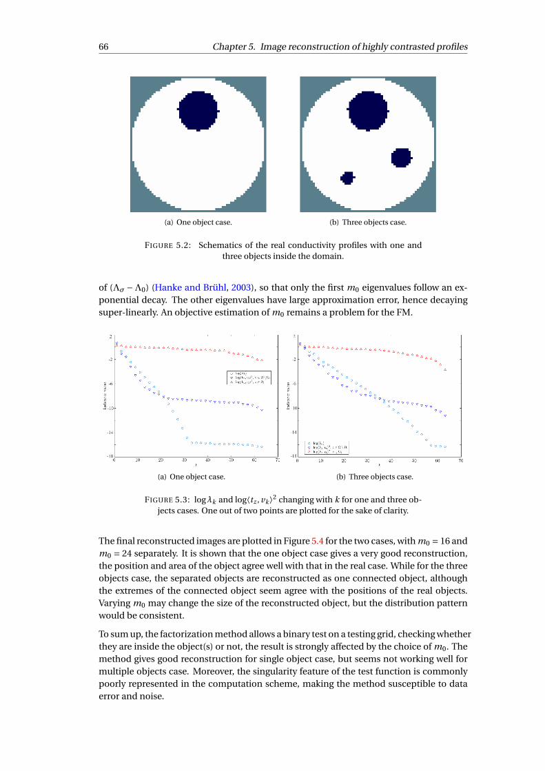
66 Chapter 5. Image reconstruction of highly contrasted profiles
(a) One object case. (b) Three objects case.
FIGURE 5.2: Schematics of the real conductivity profiles with one andthree objects inside the domain.
of (§æ°§0) (Hanke and Brühl, 2003), so that only the first m0 eigenvalues follow an ex-ponential decay. The other eigenvalues have large approximation error, hence decayingsuper-linearly. An objective estimation of m0 remains a problem for the FM.
(a) One object case. (b) Three objects case.
FIGURE 5.3: log∏k and loghtz , vki2 changing with k for one and three ob-jects cases. One out of two points are plotted for the sake of clarity.
The final reconstructed images are plotted in Figure 5.4 for the two cases, with m0 = 16 andm0 = 24 separately. It is shown that the one object case gives a very good reconstruction,the position and area of the object agree well with that in the real case. While for the threeobjects case, the separated objects are reconstructed as one connected object, althoughthe extremes of the connected object seem agree with the positions of the real objects.Varying m0 may change the size of the reconstructed object, but the distribution patternwould be consistent.
To sum up, the factorization method allows a binary test on a testing grid, checking whetherthey are inside the object(s) or not, the result is strongly affected by the choice of m0. Themethod gives good reconstruction for single object case, but seems not working well formultiple objects case. Moreover, the singularity feature of the test function is commonlypoorly represented in the computation scheme, making the method susceptible to dataerror and noise.

5.1. Review of image reconstruction methods 67
(a) One object case, m0 = 16. (b) Three objects case, m0 = 24.
FIGURE 5.4: Image reconstructions using the FM for one and three ob-jects cases.
MUSIC algorithm
The MUltiple-SIgnal-Classification (MUSIC) algorithm is based on the same mathemati-cal basis with the factorization method, while it only gives possible locations of inhomo-geneities inside the domain. In MUSIC algorithm, the inhomogeneities are consideredhaving the form ≠i = zi +"0ri≠ with zi 2≠, i = 1, · · · , p the centers of small disc-shapedinhomogeneities≠i , "0ri the radius of≠i , where "0 > 0 is a common coefficient for all≠i
and ri > 0 can be different for each inhomogeneity (Hanke and Brühl, 2003). With theseassumption, the MUSIC algorithm emphasizes the center zi of inhomogeneity.
In this context, the criteria in Eqn. (5.26) is modified as computing the angle µz betweentz and R f (§æ°§0)1/2 by:
cotµz º kP±n tzk2/k(I °P±n )tzk2, (5.31)
where
kP±n tzk2 =n0X
k=1htz , vki2 and k(I °P±n )tzk2 =
X
k=n0+1htz , vki2, (5.32)
with n0 the index of the minimum eigenvalue corresponding to the noise level ±n . Thecotµz at each grid point z can be calculated, its value indicates the possibility of the pres-ence of inhomogeneity, which should not be mistaken as the conductivity value.
Image reconstructions of the MUSIC algorithm for the two cases concerned are plottedin Figure 5.5, the noise level considered is ±n = 4 £ 10°4 and ±n = 5 £ 10°6, separately.As we can see, the positions of the objects (represented by the discrete peaks) are wellreconstructed for both cases. Noting that the size information in the reconstructed imagesis not relevant to the physical sizes of the objects, only the discrete peak values representthe presence of objects.
Additionally, the influences of measurement noise on the reconstructions of the FM andMUSIC methods have been studied. The noisy data is obtained by adding 40 dB of ran-dom noise to the image data Vi . The values of log∏k and loghtz , vki2 are plotted versusthe index k for two selected points z 2≠i and z 2≠ \≠i , as in Figure 5.6. Comparing tothe plots in Figure 5.3, it is found that much less number of eigenvalues can be used forreconstruction, which is m0 = 6 and m0 = 10 separately for the two cases.

68 Chapter 5. Image reconstruction of highly contrasted profiles
(a) One object case. (b) Three objects case.
FIGURE 5.5: Reconstructions using the MUSIC algorithm for one andthree objects cases.
(a) One object case. (b) Three objects case.
FIGURE 5.6: log∏k and loghtz , vki2 associated with noisy data for one andthree objects cases. One out of two points are plotted for the sake of clarity.
The associated image reconstructions are shown in Figure 5.7 using the FM and MUSICmethods, m0 = 6 and m0 = 8 are taken separately for the two cases in the FM, while±n = 10°2 and ±n = 5£ 10°3 for MUSIC algorithm. It is shown that the reconstructionsfrom the FM are severely distorted by the noisy data, the area estimation of the objectshas a great error for both cases. The MUSIC algorithm gives a good position estimationfor one object case, while for three objects case only the position of the largest objectis identifiable. Overall, the FM and MUSIC methods are both sensitive to measurementnoise, 40 dB of noise can depreciate the resulting images.
5.1.4 Topological sensitivity
The concept of topological sensitivity firstly appeared in the context of topological op-timization of mechanical structure (Eschenauer et al., 1994). The aim is to quantify theperturbation of an objective function with respect to a small object ≠"(a) at location aassociated with a characteristic radius ". The object ≠"(a) has Neumann or transmissionconditions on the boundary @≠"(a), and it is the only perturbation to a known referencebackground.
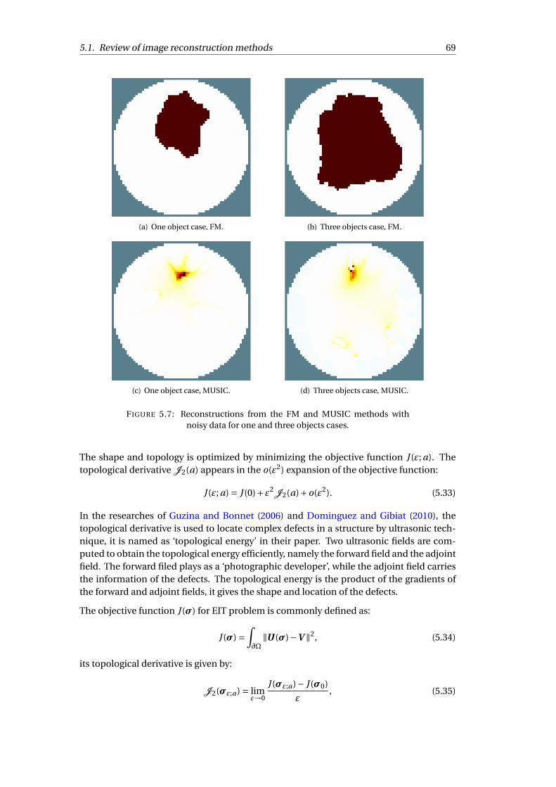
5.1. Review of image reconstruction methods 69
(a) One object case, FM. (b) Three objects case, FM.
(c) One object case, MUSIC. (d) Three objects case, MUSIC.
FIGURE 5.7: Reconstructions from the FM and MUSIC methods withnoisy data for one and three objects cases.
The shape and topology is optimized by minimizing the objective function J ("; a). Thetopological derivative J2(a) appears in the o("2) expansion of the objective function:
J ("; a) = J (0)+"2J2(a)+o("2). (5.33)
In the researches of Guzina and Bonnet (2006) and Dominguez and Gibiat (2010), thetopological derivative is used to locate complex defects in a structure by ultrasonic tech-nique, it is named as ‘topological energy’ in their paper. Two ultrasonic fields are com-puted to obtain the topological energy efficiently, namely the forward field and the adjointfield. The forward filed plays as a ‘photographic developer’, while the adjoint field carriesthe information of the defects. The topological energy is the product of the gradients ofthe forward and adjoint fields, it gives the shape and location of the defects.
The objective function J (æ) for EIT problem is commonly defined as:
J (æ) =Z
@≠kU (æ)°V k2, (5.34)
its topological derivative is given by:
J2(æ";a) = lim"!0
J (æ";a)° J (æ0)"
, (5.35)

70 Chapter 5. Image reconstruction of highly contrasted profiles
with æ";a and æ0 the conductivity profile with and without the object≠"(a). J (æ) is mini-mized through searching for J2(æ";a) < 0, i.e. in a gradient descend approach.
The adjoint method is also applicable to EIT to compute the topological derivative J2(æ";a).Considering an EIT system with four electrodes and unit disc domain, three cases are sim-ulated to obtain the topological derivative, as shown in Figure 5.8. The simulation modelhas two electrodes for current excitations, and the other two for absolute voltage mea-surements, the background has a uniform conductivity, while the object has a nearly zeroconductivity.
FIGURE 5.8: Schematic of measurment, reference and adjoint configura-tions simulated, Eexc represents the excitation electrode.
The reference configuration has a homogeneous domain, current excitations are exertedon two adjacent electrodes Eexc , voltages are measured on the others, giving the boundarymeasurements Vr e f and the potential field u0. The measurement configuration has oneobject inside ≠, the same excitation and measurement patterns are applied as in the ref-erence configuration, giving the boundary measurements Vi mg . Finally, the adjoint con-figuration uses the homogeneous medium as in the reference, while the current sourcesare exerted on the measurement electrodes in the former cases, the amplitudes are takenas (Vr e f °Vi mg ), giving the associated potential field uad j , i.e.
r · (æ0ruad j ) = 0, in≠,
æ0ruad j ·n =Vr e f °Vmeas , on excitation electrodes. (5.36)
The topological derivative J2(æ";a) is computed by:
J2(æ";a) =ru0 ·ruad j , in≠. (5.37)
A simple case with a single object of radius 0.1 inside the domain has been studied, theconductivity profile is shown in Figure 5.9(a). The associated reference, measurementand adjoint configurations are computed, giving the topological derivative shown in Fig-ure 5.9(b). As we can see, the topological derivative distribution is hard to interpret, itcannot give meaningful information about the object.
Recent researches in Bonnet (2009); Bonnet and Cakoni (2019) prove mathematically thatthe o("2) expansion of the objective function is not sufficient to retrieve the shape andtopology of an object in EIT problem, because it is not unique regarding ≠"(a). They es-tablished the o("4) approximation of J ("; a) as in Eqn. (5.38), to achieve the uniqueness.Numerical tests were performed to identify small objects at given locations, shapes and
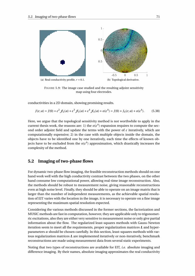
5.2. Imaging of two-phase flows 71
(a) Real conductivity profile, r = 0.1. (b) Topological derivative.
FIGURE 5.9: The image case studied and the resulting adjoint sensitivitymap using four electrodes.
conductivities in a 2D domain, showing promising results.
J ("; a) = J (0)+"2J2(a)+"3
J3(a)+"4J4(a)+o("4) = J (0)+ J4("; a)+o("4). (5.38)
Here, we argue that the topological sensitivity method is not worthwhile to apply in thecurrent thesis work, the reasons are: 1) the o("4) expansion requires to compute the sec-ond order adjoint field and update the terms with the power of " iteratively, which arecomputationally expensive; 2) in the case with multiple objects inside the domain, theobjects have to be identified one by one iteratively, each time the effects of known ob-jects have to be excluded from the o("4) approximation, which drastically increases thecomplexity of the method.
5.2 Imaging of two-phase flows
For dynamic two-phase flow imaging, the feasible reconstruction methods should on onehand work well with the high conductivity contrast between the two phases, on the otherhand consume low computational power, allowing real-time image reconstruction. Also,the methods should be robust to measurement noise, giving reasonable reconstructionseven at high noise level. Finally, they should be able to operate on an image matrix that islarger than the number of independent measurements, as the achievable spatial resolu-tion of EIT varies with the location in the image, it is necessary to operate on a fine imagerepresenting the maximum spatial resolution expected.
Considering the various methods discussed in the former sections, the factorization andMUSIC methods are fast in computation, however, they are applicable only to trigonomet-ric excitations, also they are either very sensitive to measurement noise or only give partialinformation about the flow. The regularized least-squares methods with Gauss-Newtoniteration seem to meet all the requirements, proper regularization matrices L and hyper-parameters Æ should be chosen carefully. In this section, least-squares methods with var-ious regularization matrices L are implemented iteratively or non-iteratively, benchmarkreconstructions are made using measurement data from several static experiments.
Noting that two types of reconstructions are available for EIT, i.e. absolute imaging anddifference imaging. By their names, absolute imaging approximates the real conductivity

72 Chapter 5. Image reconstruction of highly contrasted profiles
distribution in the imaging domain, while difference imaging reconstructs changes in theconductivity between the measurements at two time instants, using the difference databetween them. Difference imaging is favorable to two-phase flow measurement, wherethe conductivity changes between the present instant and the reference instant with ho-mogeneous distribution is of interest, in addition, the reference measurements are fea-sible in this context. It could circumvent modeling errors arise from the mismatch ofgeometrical configurations and the presence of contact impedance, which may degradethe image accuracy, or even lead to incorrect results. In the following sections differenceimaging is applied, the conductivity difference ¢æ is plotted in the reconstructed images.
5.2.1 2D or 3D reconstruction
The regularized least-squares methods are applicable to both 2D and 3D reconstructions,leading to three different reconstruction strategies, namely, 3D reconstruction, 2.5D re-construction, and 2D reconstruction. A number of EIDORS built-in functions are used torealize these strategies, mainly including the calc_jacobian function to compute the Jaco-bian matrix J of 2D or 3D finite element model, and several functions to generate variousregularization matrices L, such as prior_noser, prior_tikhonov and prior_laplace. The as-sociated inverse solvers inv_solve_diff_GN_one_step and inv_solve_GN are employed tocarry out one-step or iterative Gauss-Newton methods separately.
3D reconstruction
It is intuitive to implement 3D image reconstruction in EIT because of its 3D sensing do-main, the conductivity changes in the voxels are reconstructed. Usually the 3D recon-struction model is with the same geometry as the test section used for experiments, acoarse mesh is generated on the model to reduce the computation effort, on which theJacobian matrix J and various regularization matrices L are calculated. The images canbe reconstructed iteratively or non-iteratively. Numerical simulations have been carriedto demonstrate this strategy.
To begin with, a forward model is built, as shown in Figure 5.10(a), to compute the bound-ary measurements of image and reference cases. The model has the same geometry pa-rameters than in the test section of ProME-T system with ES2 electrodes, the diameter is51 mm with a height of 270 mm, the electrode size is 5 mm in height and 4 mm in circum-ferential width. The simulations in Section 2.2.3 concerning the 3D effect prove that thelongitude extend of the sensing domain is within a diameter for a small electrode size,therefore the 3D model takes a height of 100 mm to reduce the computation power. Atetrahedral mesh is generated with 36103 nodes for accurate computations of the bound-ary measurements, the mesh is refined near the electrodes. Full-scan strategy is exertedwith unit excitation amplitude, the reference measurements Vh are computed with a unitconductivity in the geometry. An object with a radius of 10 mm and conductivity nearly 0is added to the electrode plane, giving the image measurements Vi . A slice is taken acrossthe electrode plane to better display the configuration, as shown in Figure 5.10(b), theelectrodes are in green, the object in blue has significantly low conductivity, its boundaryis stressed in red.
The inverse model is built with a coarse mesh of 2499 nodes generated on the same ge-ometry as of the forward model, on which the J and L are computed for 3D image recon-struction. Applying the NOSER method, the conductivity difference is given by Eqn. (5.11)
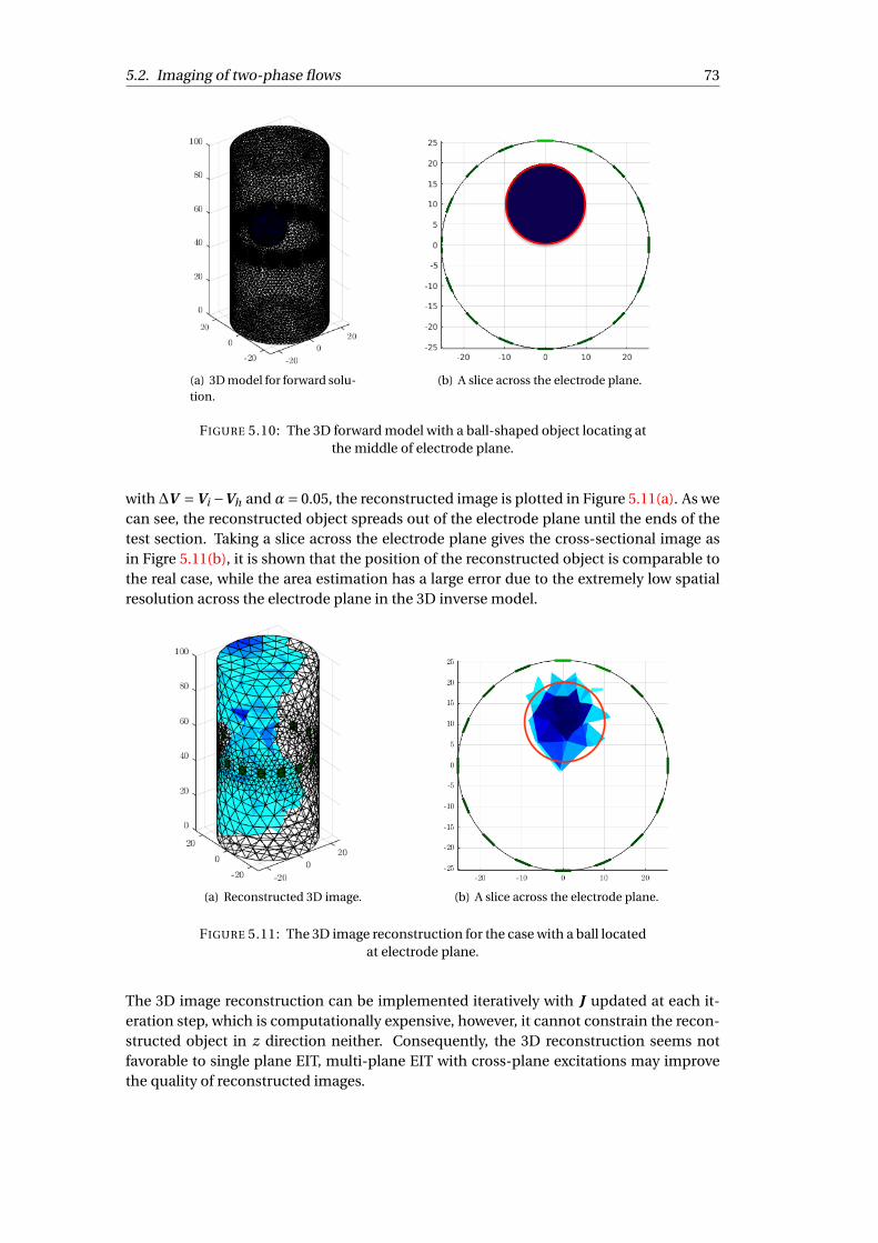
5.2. Imaging of two-phase flows 73
(a) 3D model for forward solu-tion.
(b) A slice across the electrode plane.
FIGURE 5.10: The 3D forward model with a ball-shaped object locating atthe middle of electrode plane.
with¢V =Vi °Vh andÆ= 0.05, the reconstructed image is plotted in Figure 5.11(a). As wecan see, the reconstructed object spreads out of the electrode plane until the ends of thetest section. Taking a slice across the electrode plane gives the cross-sectional image asin Figre 5.11(b), it is shown that the position of the reconstructed object is comparable tothe real case, while the area estimation has a large error due to the extremely low spatialresolution across the electrode plane in the 3D inverse model.
(a) Reconstructed 3D image. (b) A slice across the electrode plane.
FIGURE 5.11: The 3D image reconstruction for the case with a ball locatedat electrode plane.
The 3D image reconstruction can be implemented iteratively with J updated at each it-eration step, which is computationally expensive, however, it cannot constrain the recon-structed object in z direction neither. Consequently, the 3D reconstruction seems notfavorable to single plane EIT, multi-plane EIT with cross-plane excitations may improvethe quality of reconstructed images.

74 Chapter 5. Image reconstruction of highly contrasted profiles
2.5D reconstruction
Results of the 3D reconstruction show that only the slice across the electrode plane givesmeaningful information about the conductivity profile (see Figre 5.11), stimulating theidea of 2.5D reconstruction. Similar to the 3D reconstruction, the 2.5D reconstructionstarts from a 3D inverse model, while it projects the 3D model onto a 2D model beforeperforming image reconstruction. A key step is to construct a fine to coarse mapping from3D model to 2D model, assuming that the profile is invariant in z direction.
A possible way to construct this mapping is directly projecting the 3D inverse matrix ontoa pseudo-2D inverse matrix, as presented in the Algorithme de Tomographie en 3D NOSERet Aplanissement (AT3NA) (Dupré, 2017). The pseudo-2D plane is subdivided into a Carte-sian grid of certain size, considering one pixel in the grid, its extrusion along the z direc-tion generates a parallelepiped. The inverse matrices of the voxels in the 3D inverse modellocated inside the parallelepiped contribute to the inverse matrix of this pixel, their sum-mation defines the pseudo-2D inverse matrix. To achieve a reliable projection, the 3Dinverse model should be sufficiently fine (unlike in 3D reconstruction), requiring a highcomputation power to obtain J and L. Here, a fine mesh with 36103 nodes is used, asshown in Figure 5.12(a). The inverse matrix is computed using the NOSER method, thenprojected onto a coarse 2D grid of size 39£39. The reconstructed image is shown in Fig-ure 5.12(b), it presents a highly smoothing image, the position of the reconstructed objectis pushed toward the pipe boundary comparing to the real case, due to the projection of3D sensing domain into 2D.
(a) 3D inverse model with finemesh.
(b) 2.5D image reconstruction.
FIGURE 5.12: The 3D fine inverse model used for 2.5D reconstruction andthe final reconstructed image.
Both the 3D and 2.5D reconstructions require to compute J and L based on 3D modelswith large number of meshing elements, especially the 2.5D reconstruction requires a fine3D mesh, making it difficult to be implemented iteratively. Typically, they are applied inone-step Gauss-Newton methods with Tikhonov type regularizations. The advantage isthat the inverse matrix can be computed and saved in prior, enabling real-time imagereconstruction.

5.2. Imaging of two-phase flows 75
2D reconstruction
Unlike the 3D and 2.5D reconstructions, the 2D reconstruction operates on a 2D inversemodel, the difference data from 3D simulations or experiments are used directly for re-constructions: the 3D effect of the sensitivity field is not considered. Benefiting from thelow number of meshing elements, 2D image reconstruction can be performed iterativelyat acceptable computational cost. A triangle mesh with 719 meshing nodes is used in 2Dinverse model, as shown in Figure 5.13, the mesh is refined near the boundary (especiallythe electrodes) to support the high sensitivity nearby.
FIGURE 5.13: 2D inverse model with coarse mesh used for image recon-struction.
The reconstructed images associated with Vh and Vi are shown in Figure 5.14, applyingiterative methods with Tikhonov and TV regularizations, respectively. The maximum iter-ation step is set to 10 for both regularizations. In the figures, the real object is representedby the red circle, it seems that the center of the reconstructed object is pushed towardthe boundary in both methods. Additionally, Tikhonov regularization gives smoothed re-construction, while TV regularization gives sharp contrast and an over constrained areaestimation.
(a) Iterative Tikhonov method. (b) Iterative TV method.
FIGURE 5.14: 2D reconstructions using iterative Tikhonov and TV regular-ized methods and 3D measurement data.
For comparison, the 2D reconstructions using the same inverse model, but 2D boundarymeasurements have been carried out. The 2D boundary measurements are computed

76 Chapter 5. Image reconstruction of highly contrasted profiles
using the 2D forward model same as in Section 3.2.2. The object has the same positionand radius as in Figure 5.10(b). The final 2D reconstructions are shown in Figure 5.15using iterative methods with Tikhonov and TV regularizations, respectively. Comparing tothe results in Figure 5.14, it is found that 2D reconstructions with 2D measurement datagive more accurate estimations of the position and area of the reconstructed object.
(a) Iterative Tikhonov method. (b) Iterative TV method.
FIGURE 5.15: 2D reconstructions using iterative Tikhonov and TV regu-larized methods and 2D measurement data.
As a conclusion, the 3D reconstruction seems not suitable considering the single elec-trode plane used in the present EIT systems. The 2.5D reconstruction gives smoothedreconstruction, while the position and area of the reconstructed object are identifiable,also it has the advantage to perform online image reconstruction by pre-computing the2D inverse matrix. The 2D reconstruction makes it possible for iterative reconstructionswith various regularizations, while it may be more sensitive to measurement noise.
GREIT reconstruction
Except for the conventional regularization methods, it is of interest to investigate the GREITmethod for two-phase flow imaging. Here, the GREIT method is applied to reconstructthe two cases considered. A 3D GREIT model is established using the same geometry asin Figure 5.12(a) with 17604 meshing nodes. A small target with a diameter of 0.1D (Dis the domain diameter) is placed randomly inside the domain, giving the associated in-verse matrix and various performance metrics (see Section 5.1.2). The best inverse matrixR is estimated on a 2D structured mesh, through optimizing the performance metrics ofnt such targets, typically nt is chosen between 1000 to 10000. The reconstructed image isobtained multiplying the best R with the measurement differences¢V =Vi °Vh , as shownin Figure 5.10(a) for nt = 1000 and 3000, separately. As we can see, GREIT method givesvery good estimations of the position and area of the object, although smoothing effectpresents. Besides, the reconstruction with nt = 3000 gives a better area estimation closerto the real case.

5.2. Imaging of two-phase flows 77
(a) nt = 1000. (b) nt = 3000.
FIGURE 5.16: 2D GREIT reconstructions using the best inverse matrix Restimated from nt = 1000 and nt = 3000 small targets.
5.2.2 Benchmark reconstruction of static experiments
Here, the selected image reconstruction methods, namely the 2.5D NOSER method, 2Diterative methods with Tikhonov and TV regularizations, and 2D GREIT method, are ap-plied to the image reconstructions of several static experiments. The experimental datawere acquired by the ProME-T system implementing full-scan strategy. Both the two setsof electrodes ES1 and ES2 have been used, with plastic rod(s) placed in the test sectionsimulating the insulating bubbles. The conductivity distributions studied include: i) asingle rod in the center of the test section; ii) a single rod near the boundary; iii) two rodsplaced oppositely.
The reconstructed images with ES1 electrodes are shown in Figure 5.17 to 5.19 for the threecases concerned, with ES2 electrodes are shown in Figure 5.20 and 5.21, only the first twocases are studied. In the figures the difference conductivity ¢æ is plotted, the positionsand radius of the rods used in the corresponding experiments are presented by the redcircles.
(a) 2.5D NOSER method. (b) 2D iterative Tikhonovmethods.
(c) 2D iterative TV meth-ods.
(d) 2D GREIT method.
FIGURE 5.17: Image reconstructions using selected methods for static ex-periments with ES1 electrodes, center rod case.
Generally, the image reconstructions with ES1 electrodes agree well with the real casesfor all the four methods, the positions and areas are well estimated, except that the 2.5Dreconstruction gives highly smoothed images. Specifically, the GREIT has a very good per-formance for all the three cases, while the 2D iterative reconstructions give considerable

78 Chapter 5. Image reconstruction of highly contrasted profiles
(a) 2.5D NOSER method. (b) 2D iterative Tikhonovmethods.
(c) 2D iterative TV meth-ods.
(d) 2D GREIT method.
FIGURE 5.18: Image reconstructions using selected methods for static ex-periments with ES1 electrodes, boundary rod case.
(a) 2.5D NOSER method. (b) 2D iterative Tikhonovmethods.
(c) 2D iterative TV meth-ods.
(d) 2D GREIT method.
FIGURE 5.19: Image reconstructions using selected methods for static ex-periments with ES1 electrodes, two rods case.
(a) 2.5D NOSER method. (b) 2D iterative Tikhonovmethods.
(c) 2D iterative TV meth-ods.
(d) 2D GREIT method.
FIGURE 5.20: Image reconstructions using selected methods for static ex-periments with ES2 electrodes, center rod case.
artifacts for the two rods case. As to the ES2 electrodes, the 2.5D and GREIT methodsseem promising, while the 2D iterative methods give large errors in both position andarea estimations. Possible reasons include: i) the high noise level associated with the ES2electrodes due to the low measurement amplitude; ii) the pseudo-2D experimental con-figurations with long rods inserted in the test section favor the long electrodes in ES1.
5.3 Quantitive comparisons of various excitation strategies
In this section, we focus specifically on the role of the excitation strategy itself on thereconstructed images. The images obtained for the excitation strategies considered are

5.3. Quantitive comparisons of various excitation strategies 79
(a) 2.5D NOSER method. (b) 2D iterative Tikhonovmethods.
(c) 2D iterative TV meth-ods.
(d) 2D GREIT method.
FIGURE 5.21: Image reconstructions using selected methods for static ex-periments with ES2 electrodes, boundary rod case.
compared numerically for different reference conductivity profiles. Different criteria areproposed for quantitive comparisons, including the global error in the identification ofthe conductivity field and geometrical errors in the reconstruction of the sought object(s)(area and position). Moreover, two types of regularizations are applied in the reconstruc-tion process, namely the Tikhonov regularization and the TV regularization. A set of to-mographic images are compared, corresponding to static experiments carried out withstill water and plastic rod(s) as the object(s) to be reconstructed.
The two reconstruction methods considered here are: (i) the NOSER method, which con-strains the image amplitude and for which regularization is performed through penaliza-tion by the diagonal elements of the Jacobian matrix J ; (ii) an iterative method with TVregularization, which tends to preserve discontinuities in the reconstructed conductiv-ity distribution thus leading to reconstructions with sharp contrasts (Borsic et al., 2009).The GREIT method is not used in the current section since we consider the effects of theexcitation strategy itself on the reconstructions, so that it is more reasonable to employconventional reconstruction methods.
For various excitation strategies, a value of Æ is decided for each reconstruction methodthrough the L-curve method in a preliminary analysis with a reference object, then usedin corresponding image reconstructions. In regularization methods, we have the fidelityterm and the penalty term, the L-curve method plots the values of the penalty term againstthat of the fidelity term for a series of Æ values. In current research, an object with a ra-dius of 0.05 and a nearly zero conductivity located at the halfway along the radius of theunit disc domain is used to obtain the optimal Æ. The L-curves for full-scan strategy withNOSER regularization is plotted in Figure 5.22, 40 values of Æ ranging from 10°6 to 0.5 areapplied. As we can see, we have the ‘L’ shape in which the optimalÆ is located at the pointof maximum curvature, which corresponds to ƺ 0.1 in this case.
5.3.1 From synthetic data
Five different objective conductivity distributions ætrue are considered in a finite elementsetting. The background medium is a disk with unit diameter endowed with conductivityof 1.0, which contains one or two low conductivity objects with conductivity 0.1. Theseobjects are circular, with radius r and distance d to the origin, and the case defining valuesare reported in Table 5.1. For such configurations, both the forward and inverse problemsare solved using EIDORS, with the two reconstruction methods described previously.

80 Chapter 5. Image reconstruction of highly contrasted profiles
FIGURE 5.22: The L-curve for full-scan strategy with NOSER method. Thepoint at maximum curvature corresponds to the optimal hyperparameter.
TABLE 5.1: Geometric parameters defining the cases considered with thecircular object(s) to be reconstructed.
Case 1 2 3 4 5
r 0.2 0.7 0.2 [0.25 0.15] [0.25 0.15]d 0 0 0.7 [0 0.7] [0.5 0.7]
Reconstructed images
The obtained images, i.e. the reconstructed conductivity contrasts ¢æid = (æid ° 1), forthe various excitation strategies considered are shown in Table 5.2 for both the NOSERmethod and TV regularization. In each case, the object(s) are correctly identified quali-tatively, but their sizes is not systematically constrained quantitatively, see the cases 1, 2and 4. In terms of excitation strategy, the full-scan and trigonometric strategies seem toconstrain the object(s) size(s) more than the others, but they may lead to artifacts in thereconstructions, see the cases 4 and 5.
The profiles of the reconstructed conductivity distributions are extracted along one diam-eter and plotted in the Figures 5.23 and 5.24 for the cases 1 and 4 respectively. The trueobjects to be reconstructed are indicated by the grey regions. These results highlight thatthe full-scan and trigonometric strategies lead systematically to images with higher con-ductivity contrasts compared to the others approaches. For Case 1, the opposite strategyleads to the least accurate reconstructions, in terms of object size and conductivity con-trast, which agrees with the earlier statement that its resolution is limited by its relativelylow number of independent measurements. It gives also unsatisfactory reconstructions inCase 4, with the concentric object being smooth out in the obtained image, thus makingit difficult to discriminate the two objects. In comparison, the full-scan and trigonomet-ric strategies give better reconstructions in Case 1, in terms of conductivity contrast andobject size, as well as in Case 4, with the two objects being clearly distinguished.
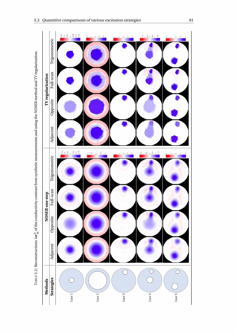
5.3. Quantitive comparisons of various excitation strategies 81
TA
BL
E5.
2:R
econ
stru
ctio
ns¢æ
h idof
the
con
duct
ivit
yco
ntr
astf
rom
syn
thet
icm
easu
rem
ents
and
usi
ng
the
NO
SER
met
hod
and
TV
regu
lari
zati
on.
Met
hod
sN
OSE
Ron
est
epT
Vre
gula
riza
tion
Stra
tegi
esA
djac
ent
Op
pos
ite
Full-
scan
Trig
onom
etri
cA
djac
ent
Op
pos
ite
Full-
scan
Trig
onom
etri
c

82 Chapter 5. Image reconstruction of highly contrasted profiles
(a) NOSER method. (b) TV regularization.
FIGURE 5.23: [Case 1] Profiles of the reconstructed conductivity contrasts¢æh
id along one diameter for the different excitation strategies and recon-struction methods considered.
(a) NOSER method. (b) TV regularization.
FIGURE 5.24: [Case 4] Profiles of the reconstructed conductivity contrasts¢æh
id along one diameter for the different excitation strategies and recon-struction methods considered.
Quantitative indicators
This section focuses on a quantitative evaluation of the quality of the reconstructed im-ages of Section 5.3.1. To do so, three criteria are introduced and evaluated on the obtainedimages.
Global identification error. An error indicator ≤id is defined as the overall relative recon-struction error on the conductivity field. In the discrete setting considered, it is definedas:
≤id = 1A
NelX
ne=1
|æid(ne )°ætrue(ne )|ætrue(ne )
Ael(ne ), with A =NelX
ne=1Ael(ne ), (5.39)
where the summation is performed over elements, whose total number is Nel and giventheir individual area Ael(ne ). The indicator ≤id is computed for all of the reconstructedimages of Table 5.2. For each case and each reconstruction method, the values ≤id arenormalized by the largest error among the four excitation strategies and their logarithm

5.3. Quantitive comparisons of various excitation strategies 83
is then plotted in Figure 5.25. In such a figure, low values indicate good relative perfor-mances.
The opposite strategy is almost systematically associated with the largest identificationerrors (with the normalized value 1 giving a zero logarithmic value). The adjacent methodperforms quite well on average while the full-scan and trigonometric strategies lead tocomparable but lightly less accurate reconstructions overall. Yet, it should be noted thata low value ≤id does not necessarily implies that the object(s) are correctly identified ge-ometrically, see e.g. the reconstructions of Figure 5.24(b). Therefore, one considers nexttwo additional indicators of the geometrical errors on the reconstructed objects.
FIGURE 5.25: Logarithm of the global identification errors ≤id, normal-ized by the largest error among the four excitation strategies for eachcase and each reconstruction method. The value 0 is associated with thelowest-performing strategy and low values indicate relatively better per-
formances.
Geometrical area error. In EIT, the boundaries of highly contrasted objects are notori-ously smooth out in reconstructed images. While total variation regularization can rem-edy to that, in certain applications, such as two-phase flow imaging, the phase fractionis a critical parameter to estimate. In such situations, the reconstructed conductivity æid
can be further segmented into æid as:
æid =
8<
:°1 if ¢æid ∑ 1
4min¢æid
0 otherwise,(5.40)
where 1/4 is actually a user-chosen value. Doing so, a geometrical area error ≤A is definedas:
≤A = |Aid ° Atrue|Atrue
, (5.41)
where Aid and Atrue are respectively the area of the object(s), i.e. the region(s) of lowestconductivity, in the segmented reconstruction and in the true image, respectively. Theerror indicator ≤A is computed for all of the reconstructed images of Table 5.2. As done for

84 Chapter 5. Image reconstruction of highly contrasted profiles
the global identification error, normalization by the largest error among the four excitationstrategies is employed for each case and each reconstruction method. Logarithmic valuesare then plotted in Figure 5.26.
According to this indicator, both the adjacent and opposite strategies perform poorly, onaverage, in identifying the phase fraction in the cases considered. In contrast, the per-formances of the full-scan and trigonometric strategies are relatively comparable to eachother and significantly better than the former ones. This sheds a new light on the resultsof Figure 5.25, as a low global identification error value is not necessarily associated withan inaccurate geometric reconstruction of the targeted object(s).
FIGURE 5.26: Logarithm of the geometrical area errors ≤A, normalizedby the largest error among the four excitation strategies for each caseand each reconstruction method. The value 0 is associated with thelowest-performing strategy and low values indicate relatively better per-
formances.
Positioning error. A third criterion is finally introduced to evaluate the accuracy of theobject(s) position(s) in the reconstructed æid distribution. As in some cases the objectsconnectedness can be difficult to assess in the reconstructed images, one focuses only onthe objects barycenter. Doing so, one introduces the positioning error ≤p as:
≤p = |did °dtrue|D
, (5.42)
with did and dtrue being the distance of the objects barycenter to the origin in the recon-structed and true image, respectively, while D is the diameter of the domain. As done withthe two error indicators considered previously, normalization by the largest error amongthe four excitation strategies is employed for each case and each reconstruction method.Logarithmic values are then computed and the results are plotted in Figure 5.27.

5.3. Quantitive comparisons of various excitation strategies 85
According to this third geometrical criterion, the adjacent strategy is associated with largesystematic errors. The performances of the opposite, full-scan and trigonometric strate-gies are relatively comparable to each other. In some cases, the full-scan and trigono-metric strategies seem to yield reconstructions that are slightly more accurate than theopposite strategy.
FIGURE 5.27: Logarithm of the positioning errors ≤p, normalized bythe largest error among the four excitation strategies for each case andeach reconstruction method. The value 0 is associated with the lowest-performing strategy and low values indicate relatively better perfor-
mances.
5.3.2 From experimental data
In this last section, a number of image reconstructions from experimental data are pro-vided. The experiments are static tests conducted using the ProME-T system with ES1electrodes. The system has 16 electrodes and a RE of 50-60 dB, from which the numericalresults are evaluated with the noisy experimental data. Low conductive plastic rods wereplaced in a test section filled with water to create the objective conductivity maps to bereconstructed. The system operates using the full-scan excitation strategy, which allowsus to extract the measurement data for the adjacent and opposite strategies. Note that theimplementation of the trigonometric strategy is currently beyond the technical capabili-ties of this system as it would require an upgrade with additional acquisition cards. There-fore, the latter strategy is not considered in this section, but the reader can refer to, e.g.Cook et al. (1994, Figure 11) and Newell et al. (1993, Figure 5.3), for typical reconstructedimages from experimental data using the trigonometric strategy for configurations thatare comparable to these considered here.
In the experimental setting, the test section has height of 270 mm and diameter of 51 mm,the static experiments can therefore be considered as pseudo-2D, which allows us to usethe same reconstruction methods as the Section 5.3.1. The reconstructed images are pro-vided in Table 5.3 for experimental configurations that correspond to the cases 1, 3 and 5

86 Chapter 5. Image reconstruction of highly contrasted profiles
of Section 5.3.1. In combination with the quantitative results of Section 5.3.1, the imagereconstructions from experimental data tend to confirm qualitatively the preeminence ofthe full-scan strategy over the two other modes.
To conclude, the adjacent, opposite, full-scan and trigonometric excitation strategies forEIT have been compared in a number of criteria, namely, complexity of a practical im-plementation, number of independent measurements, amplitude of the measured re-sponses, sensitivity distribution and quality of the final reconstructed images, see Sec-tion 3.2 and 5.3. Both numerical simulations and static experiments are employed forsuch a comparison. All of these excitation protocols are well within the reach of standardup-to-date hardware.
Considering first the practical implementation criteria synthesized in Section 3.2.4, it ap-pears that the choice of a particular excitation strategy has to be closely related to spe-cific practical constraints. For example, one might favor the quick response of the systemrather than its amplitude or sensitivity distribution. Moreover, it should be noted that thepractical criteria considered do not necessarily predict the imaging capabilities of a givenexcitation strategy. Therefore, this analysis is complemented by an evaluation of the qual-ity of reconstructed images for the different excitation strategies, both from synthetic andexperimental data in Section 5.3. Five objective conductivity maps are considered andtwo different reconstruction methods are employed. For the studied configurations, thefull-scan and trigonometric strategies lead to the best results on average, both qualita-tively and quantitatively. They allow a better geometrical reconstruction of the object(s)geometry and yield images with sharper contrasts compared to the adjacent and oppositestrategies.
The preeminence of the full-scan and trigonometric protocols is confirmed with respectto the quality of the reconstructed images. Yet, they are associated with larger acquisitiontimes or a system more complex compared to the adjacent and opposite strategies. Almeand Mylvaganam (2007) reached similar conclusions for ECT through comparing severalmeasurement protocols numerically. While these drawbacks can generally be circum-vented using modern hardware and softwares implementations (e.g. FPGA and FDM),and sufficient computational power.

5.3. Quantitive comparisons of various excitation strategies 87
TA
BL
E5.
3:R
econ
stru
ctio
ns
ofth
eco
ndu
ctiv
ity
con
tras
t¢æ
h idfr
omex
per
imen
tald
ata
and
usi
ng
the
NO
SER
met
hod
orT
Vre
gula
riza
tion
.
Met
hod
sN
OSE
Ron
est
epT
Vre
gula
riza
tion
Stra
tegi
esA
djac
ent
Op
pos
ite
Full-
scan
Adj
acen
tO
pp
osit
eFu
ll-sc
an

89
Chapter 6
Dynamic two-phase flow experiments
Despite the numerous EIT systems used in two-phase flow measurements, the full-scanstrategy gives a new insight into this research field, its advantages regarding the robust-ness to measurement noise and quality of reconstructed images are evidenced (Danget al., Submitted). Additionally, taking advantage of the redundant measurements fromthe full-scan strategy, the eigenvalue-based approach has been proposed in the currentthesis study, allowing to estimate the phase fraction from the EIT raw data without im-age reconstruction. In this chapter, the comprehensive EIT measurement mode consistsof the EIT system exploiting full-scan strategy and the associated data post-processingapproaches, is applied to measure the horizontal two-phase flows in both research andindustrial loops, to perform online and offline flow imaging and extract information offlow related features, namely, the void fraction and flow regime.
Two sets of dynamic tests have been performed in different horizontal flow loops. The firstone was performed in the multiphase flow loop in the processing lab of USN by Math-ieu Darnajou during his visit, it took two days to run all the experimental series. TheONE-SHOT system was applied for flow measurements. A total of 80 experimental serieshave been conducted with various air/water mass flow rates, covering slug, plug, stratifiedsmooth, stratified wavy and annular flows. The EIT measurement data are processed andcompared with the reference measurements from other meters in the loop, the results arepresented here. The second test was performed in the BENSON loop in cooperation withthe PKL research group of Framatome GmbH. I’ve stayed there for 2 weeks to perform theexperiments, it took one week to mount and calibrate the EIT system and another weekfor experiments under various configurations. The BENSON loop is an industrial exper-iment loop with metal pipelines for high temperature high pressure two-phase flows. Atotal of 33 experimental series have been carried out at various temperatures and voidfractions. The ProME-T system with an extra acquisition card was used for dual-plane EITmeasurements with the two plans working independently, its performance under com-plex environment is assessed. The EIT data analysis provides insights on the merits anddeficiencies of the proposed measurement mode, its applicability is evaluated under lab-oratory and industrial environments.
6.1 Horizontal two-phase flow regimes
Different flow regimes may appear in a flow pipe depending on the governing mech-anisms of gas-liquid two phase flow: gravity, gas momentum, and surface tension. Itis complex to decide the flow regime by numerical simulation, the mass, momentumand energy transfer among phases are very sensitive to phase distribution. Experimen-tally, well-developed flow regimes can be parametrized by a limited set of parameters (e.g.

90 Chapter 6. Dynamic two-phase flow experiments
mass flow rate of each phase) for a given experimental setup, referring as the multiphaseflow regimes. A number of experimental (Mandhane et al., 1974) and analytical (Taiteland Dukler, 1976; Taitel et al., 1980) studies have assessed the flow regimes for variousflow conditions in horizontal, vertical and inclined configurations, leading to various flowregime maps. Specifically for horizontal gas-water two-phase flow, which is concerned incurrent thesis study, the well-developed flow regimes typically include: bubble, stratifiedsmooth, stratified wavy, plug, slug, annular and mist flows (Chen et al., 1999; Perera et al.,2017), the typology is shown in Figure 6.1. An example of flow regime map is shown inFigure 6.2.
FIGURE 6.1: Sketches of various horizontal gas-water flow regimes.
The flow regimes distinguish from each other in terms of radial and/or axial distributionof liquid and gas. In bubble flow, the gas phase is distributed as discrete bubbles in con-tinuous liquid phase, mainly gathering near the top in horizontal flow. For slug flow, mostof the gas is located in the large bullet shaped bubbles on the top, they move uniformlyalong with the continuous liquid which bridges the pipe and contains small gas bubblesbetween the slugs. Plug flow is somewhat similar to slug flow, but with large bubbles ex-isting between the plugs, instead of small gas bubbles between slugs. Stratified flow iscompletely separated with gas in the upper part and liquid in the lower part of the pipe,the interface can be smooth or wavy, giving stratified smooth and wavy flows, respectively.In annular flow, liquid forms a coat all around the pipe walls, with gas flowing in the mid-dle possibly with liquid droplets inside, usually the coat is thicker at the bottom than atthe top because of gravity effects. Mist flow is characterized by the continuous gas phasein the core of the pipe, with liquid drops dispersed in the gas core.
Flow regime identification can be realized using the signals from single or multiple sen-sors, e.g. radiation-based densitometers, impedance probe (Ahmed and Ismail, 2008),wire-mesh sensor (Schleicher et al., 2016) and electrical tomography sensors (Wang andZhang, 2009; Tan et al., 2007). The signal need to be representative to the cross-sectionalaveraging void fraction, the time series of consecutive signals contain information aboutthe flow regime. Conventionally, mathematical or statistical tools such as probability den-sity function, principal component analysis and power spectral density are used to ana-lyze the time series signal (Ahmed and Ismail, 2008; Paranjape et al., 2012). While therecent trend in flow regime identification is to use machine learning algorithms, such as
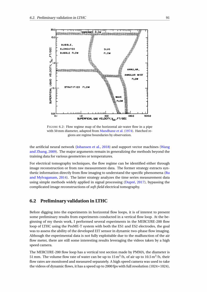
6.2. Preliminary validation in LTHC 91
FIGURE 6.2: Flow regime map of the horizontal air-water flow in a pipewith 50 mm diameter, adapted from Mandhane et al. (1974). Hatched re-
gions are regime boundaries by observation.
the artificial neural network (Johansen et al., 2018) and support vector machines (Wangand Zhang, 2009). The major arguments remain in generalizing the methods beyond thetraining data for various geometries or temperatures.
For electrical tomography techniques, the flow regime can be identified either throughimage reconstruction or from raw measurement data. The former strategy extracts syn-thetic information directly from flow imaging to understand the specific phenomena (Ruand Mylvaganam, 2014). The latter strategy analyzes the time series measurement datausing simple methods widely applied in signal processing (Dupré, 2017), bypassing thecomplicated image reconstructions of soft-field electrical tomography.
6.2 Preliminary validation in LTHC
Before digging into the experiments in horizontal flow loops, it is of interest to presentsome preliminary results from experiments conducted in a vertical flow loop. At the be-ginning of my thesis work, I performed several experiments in the MERCURE-200 flowloop of LTHC using the ProME-T system with both the ES1 and ES2 electrodes, the goalwas to assess the ability of the developed EIT sensor in dynamic two-phase flow imaging.Although the experimental data is not fully exploitable due to the malfunction of the airflow meter, there are still some interesting results leveraging the videos taken by a highspeed camera.
The MERCURE-200 flow loop has a vertical test section made by PMMA, the diameter is51 mm. The volume flow rate of water can be up to 15 m3/h, of air up to 10.5 m3/h, theirflow rates are monitored and measured separately. A high speed camera was used to takethe videos of dynamic flows, it has a speed up to 2000 fps with full resolution (1024£1024),
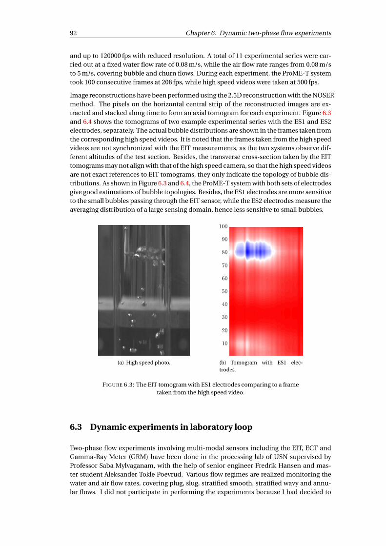
92 Chapter 6. Dynamic two-phase flow experiments
and up to 120000 fps with reduced resolution. A total of 11 experimental series were car-ried out at a fixed water flow rate of 0.08 m/s, while the air flow rate ranges from 0.08 m/sto 5 m/s, covering bubble and churn flows. During each experiment, the ProME-T systemtook 100 consecutive frames at 208 fps, while high speed videos were taken at 500 fps.
Image reconstructions have been performed using the 2.5D reconstruction with the NOSERmethod. The pixels on the horizontal central strip of the reconstructed images are ex-tracted and stacked along time to form an axial tomogram for each experiment. Figure 6.3and 6.4 shows the tomograms of two example experimental series with the ES1 and ES2electrodes, separately. The actual bubble distributions are shown in the frames taken fromthe corresponding high speed videos. It is noted that the frames taken from the high speedvideos are not synchronized with the EIT measurements, as the two systems observe dif-ferent altitudes of the test section. Besides, the transverse cross-section taken by the EITtomograms may not align with that of the high speed camera, so that the high speed videosare not exact references to EIT tomograms, they only indicate the topology of bubble dis-tributions. As shown in Figure 6.3 and 6.4, the ProME-T system with both sets of electrodesgive good estimations of bubble topologies. Besides, the ES1 electrodes are more sensitiveto the small bubbles passing through the EIT sensor, while the ES2 electrodes measure theaveraging distribution of a large sensing domain, hence less sensitive to small bubbles.
(a) High speed photo. (b) Tomogram with ES1 elec-trodes.
FIGURE 6.3: The EIT tomogram with ES1 electrodes comparing to a frametaken from the high speed video.
6.3 Dynamic experiments in laboratory loop
Two-phase flow experiments involving multi-modal sensors including the EIT, ECT andGamma-Ray Meter (GRM) have been done in the processing lab of USN supervised byProfessor Saba Mylvaganam, with the help of senior engineer Fredrik Hansen and mas-ter student Aleksander Tokle Poevrud. Various flow regimes are realized monitoring thewater and air flow rates, covering plug, slug, stratified smooth, stratified wavy and annu-lar flows. I did not participate in performing the experiments because I had decided to

6.3. Dynamic experiments in laboratory loop 93
(a) High speed photo. (b) Tomogram with ES2 elec-trodes.
FIGURE 6.4: The EIT tomogram with ES2 electrodes comparing to a frametaken from the high speed video.
attend the SWINTH-2019 workshop before scheduling the experiments, while I designedthe test matrix and post-processed the experiment data for image reconstruction and flowfeatures extraction.
In this section, EIT image reconstruction is performed using 2.5D reconstruction withthe NOSER method, through which the transverse cross-sectional images are obtained.Then, the conductivity profiles along the longitudinal section are extracted and axiallystacked along acquisition time, giving a stacked EIT tomogram for each experimental se-ries. Then, the eigenvalue-based approach proposed in Chapter 4 is applied to identify theflow regime using the eigenvalues of the normalized impedance matrix, the correlationbetween the leading eigenvalue and the reference volume averaged void fractions (AVF)is analyzed, a calibration diagram is obtained for further application. Furthermore, theestimated AVF is integrated into the EIT tomogram for a better visualization of phase dis-tribution. The experimental procedures, data processing methodology and main resultsare presented as follows.
6.3.1 Experiment procedures
Multiphase flow rig
The multiphase flow rig used for experiments is shown in Figure 6.5, it enables the injec-tion of oil, water and air in a horizontal or inclined pipe at room temperature. The injec-tion of each medium is monitored independently using the dedicated meter. The innerdiameter of the pipe is 51 mm, its thickness is 2.5 mm with a length of 15 m, the medi-ums are mixed at the inlet of the pipe so that the flow is well developed at the observationand measurement sections. The transparent PMMA section enables to determine the flowregime by visual observation or take high speed video. The ECT/EIT sensor and GRM areinstalled along the flow direction at the downstream, the data from the ECT sensor is notused in the present study. The ONE-SHOT system was used for experiments.
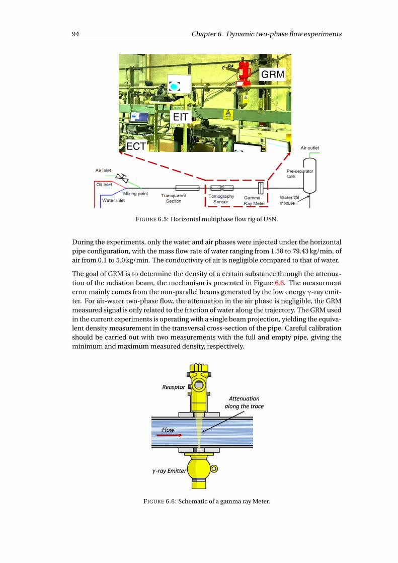
94 Chapter 6. Dynamic two-phase flow experiments
FIGURE 6.5: Horizontal multiphase flow rig of USN.
During the experiments, only the water and air phases were injected under the horizontalpipe configuration, with the mass flow rate of water ranging from 1.58 to 79.43 kg/min, ofair from 0.1 to 5.0 kg/min. The conductivity of air is negligible compared to that of water.
The goal of GRM is to determine the density of a certain substance through the attenua-tion of the radiation beam, the mechanism is presented in Figure 6.6. The measurmenterror mainly comes from the non-parallel beams generated by the low energy g-ray emit-ter. For air-water two-phase flow, the attenuation in the air phase is negligible, the GRMmeasured signal is only related to the fraction of water along the trajectory. The GRM usedin the current experiments is operating with a single beam projection, yielding the equiva-lent density measurement in the transversal cross-section of the pipe. Careful calibrationshould be carried out with two measurements with the full and empty pipe, giving theminimum and maximum measured density, respectively.
FIGURE 6.6: Schematic of a gamma ray Meter.
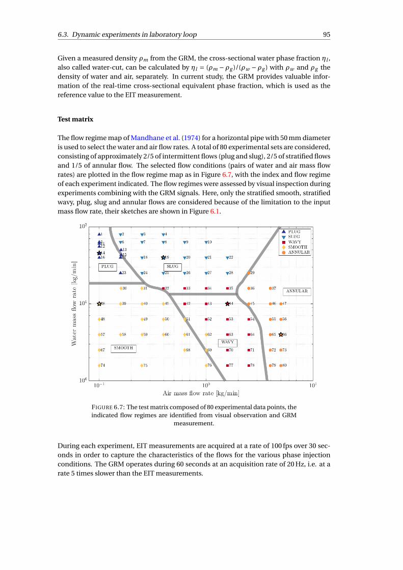
6.3. Dynamic experiments in laboratory loop 95
Given a measured density Ωm from the GRM, the cross-sectional water phase fraction ¥l ,also called water-cut, can be calculated by ¥l = (Ωm °Ωg )/(Ωw °Ωg ) with Ωw and Ωg thedensity of water and air, separately. In current study, the GRM provides valuable infor-mation of the real-time cross-sectional equivalent phase fraction, which is used as thereference value to the EIT measurement.
Test matrix
The flow regime map of Mandhane et al. (1974) for a horizontal pipe with 50 mm diameteris used to select the water and air flow rates. A total of 80 experimental sets are considered,consisting of approximately 2/5 of intermittent flows (plug and slug), 2/5 of stratified flowsand 1/5 of annular flow. The selected flow conditions (pairs of water and air mass flowrates) are plotted in the flow regime map as in Figure 6.7, with the index and flow regimeof each experiment indicated. The flow regimes were assessed by visual inspection duringexperiments combining with the GRM signals. Here, only the stratified smooth, stratifiedwavy, plug, slug and annular flows are considered because of the limitation to the inputmass flow rate, their sketches are shown in Figure 6.1.
FIGURE 6.7: The test matrix composed of 80 experimental data points, theindicated flow regimes are identified from visual observation and GRM
measurement.
During each experiment, EIT measurements are acquired at a rate of 100 fps over 30 sec-onds in order to capture the characteristics of the flows for the various phase injectionconditions. The GRM operates during 60 seconds at an acquisition rate of 20 Hz, i.e. at arate 5 times slower than the EIT measurements.

96 Chapter 6. Dynamic two-phase flow experiments
6.3.2 Eigenvalue-based approach
In this section, we expose our approach combining EIT-based image reconstructions andthe eigenvalue correlation method. The proposed flow visualization procedure is as fol-lows:
A. For the configuration considered and the EIT system employed, the correlation be-tween the mean NIM leading eigenvalue and the AVF is investigated for different flowregimes, from which a calibration diagram is constituted.
B. For a given experiment, the temporal evolution of the NIM leading eigenvalue ∏max
(i.e. ∏(16) in Chapter 4) is analyzed and associated with a raw image guess, from which theflow regime is identified.
C. Cross-sectional EIT-based raw image reconstructions are stacked axially to form atime-dependent tomogram.
D. Knowing the flow regime from B, the calibration diagram of A is used to estimate theAVF, thus leading to a threshold value that is used to binarize the EIT tomogram of C.
Remark 1 In the present study, the raw image reconstructions are computed using the NOSERmethod. Yet, the procedure above does not rely on it specifically and alternative image re-construction methods can be used as well.
Remark 2 The threshold value determined in step D is here applied to all the images alongthe time sequence, i.e. the AVF is estimated only once for a given experimental sequence.Yet, the proposed approach can be applied to each cross-sectional image, i.e. at each timestep, if necessary, with the knowledge of the current state of the flow regime.
Each of the steps of the procedure above is now detailed and illustrated on the experimen-tal data set obtained on the USN loop.
6.3.3 System calibration from NIM leading eigenvalue and AVF correlation
The Maxwell-Hewitt relation can be used to approximate the phase fraction from EIT data,see e.g. George et al. (2000). However, this relation is only applicable when the backgroundmedium is continuous and the non-conductive phase is mono-dispersed, which is not thecase for the horizontal two-phase flows considered here. Up to the Authors’ knowledge,there are only few methods reported on void fraction estimation in such configurationsbased on EIT data only. Note however that a dual-modality ECT/EIT measurement basedapproach has been used in Wang et al. (2017) for image segmentation. Here, the correla-tion between the NIM leading eigenvalue and the AVF is investigated from EIT raw data,with the reference AVF being calculated by averaging the GRM void fraction for each ex-perimental set. This leads to a system calibration diagram applicable to subsequent (i.e.unknown) flow conditions.
Given a flow regime calibration condition, a number NF of EIT measurement frames areacquired, each being associated with a normalized impedance matrix Z f . A mean NIMZmean is then computed as:
Zmean = 1NF
NFX
f =1Z f ,
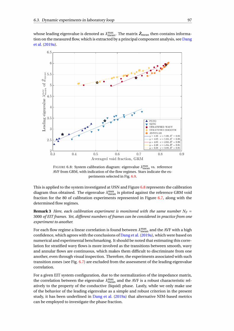
6.3. Dynamic experiments in laboratory loop 97
whose leading eigenvalue is denoted as ∏maxmean. The matrix Zmean then contains informa-
tion on the measured flow, which is extracted by a principal component analysis, see Danget al. (2019a).
FIGURE 6.8: System calibration diagram: eigenvalue ∏maxmean vs. reference
AVF from GRM, with indication of the flow regimes. Stars indicate the ex-periments selected in Fig. 6.9.
This is applied to the system investigated at USN and Figure 6.8 represents the calibrationdiagram thus obtained. The eigenvalue ∏max
mean is plotted against the reference GRM voidfraction for the 80 of calibration experiments represented in Figure 6.7, along with thedetermined flow regimes.
Remark 3 Here, each calibration experiment is monitored with the same number NF =3000 of EIT frames. Yet, different numbers of frames can be considered in practice from oneexperiment to another.
For each flow regime a linear correlation is found between ∏maxmean and the AVF with a high
confidence, which agrees with the conclusions of Dang et al. (2019a), which were based onnumerical and experimental benchmarking. It should be noted that estimating this corre-lation for stratified wavy flows is more involved as the transitions between smooth, wavyand annular flows are continuous, which makes them difficult to discriminate from oneanother, even through visual inspection. Therefore, the experiments associated with suchtransition zones (see Fig. 6.7) are excluded from the assessment of the leading eigenvaluecorrelation.
For a given EIT system configuration, due to the normalization of the impedance matrix,the correlation between the eigenvalue ∏max
mean and the AVF is a robust characteristic rel-atively to the property of the conductive (liquid) phase. Lastly, while we only make useof the behavior of the leading eigenvalue as a simple and robust criterion in the presentstudy, it has been underlined in Dang et al. (2019a) that alternative NIM-based metricscan be employed to investigate the phase fraction.
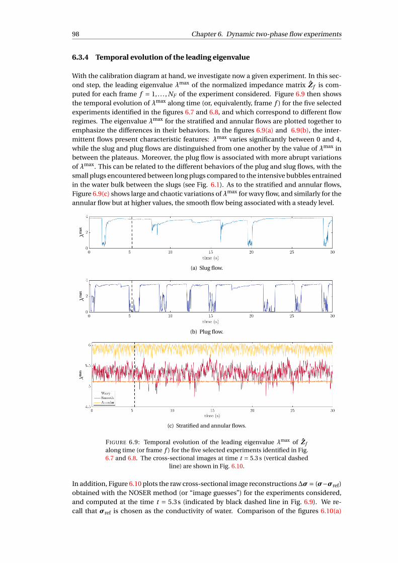
98 Chapter 6. Dynamic two-phase flow experiments
6.3.4 Temporal evolution of the leading eigenvalue
With the calibration diagram at hand, we investigate now a given experiment. In this sec-ond step, the leading eigenvalue ∏max of the normalized impedance matrix Z f is com-puted for each frame f = 1, . . . , NF of the experiment considered. Figure 6.9 then showsthe temporal evolution of ∏max along time (or, equivalently, frame f ) for the five selectedexperiments identified in the figures 6.7 and 6.8, and which correspond to different flowregimes. The eigenvalue ∏max for the stratified and annular flows are plotted together toemphasize the differences in their behaviors. In the figures 6.9(a) and 6.9(b), the inter-mittent flows present characteristic features: ∏max varies significantly between 0 and 4,while the slug and plug flows are distinguished from one another by the value of ∏max inbetween the plateaus. Moreover, the plug flow is associated with more abrupt variationsof ∏max. This can be related to the different behaviors of the plug and slug flows, with thesmall plugs encountered between long plugs compared to the intensive bubbles entrainedin the water bulk between the slugs (see Fig. 6.1). As to the stratified and annular flows,Figure 6.9(c) shows large and chaotic variations of ∏max for wavy flow, and similarly for theannular flow but at higher values, the smooth flow being associated with a steady level.
(a) Slug flow.
(b) Plug flow.
(c) Stratified and annular flows.
FIGURE 6.9: Temporal evolution of the leading eigenvalue ∏max of Z falong time (or frame f ) for the five selected experiments identified in Fig.6.7 and 6.8. The cross-sectional images at time t = 5.3 s (vertical dashed
line) are shown in Fig. 6.10.
In addition, Figure 6.10 plots the raw cross-sectional image reconstructions¢æ= (æ°æref)obtained with the NOSER method (or “image guesses”) for the experiments considered,and computed at the time t = 5.3s (indicated by black dashed line in Fig. 6.9). We re-call that æref is chosen as the conductivity of water. Comparison of the figures 6.10(a)
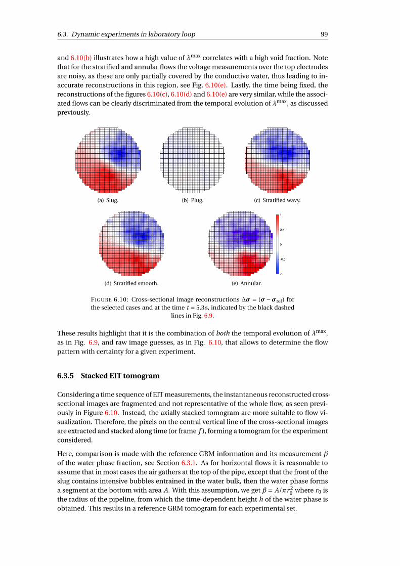
6.3. Dynamic experiments in laboratory loop 99
and 6.10(b) illustrates how a high value of ∏max correlates with a high void fraction. Notethat for the stratified and annular flows the voltage measurements over the top electrodesare noisy, as these are only partially covered by the conductive water, thus leading to in-accurate reconstructions in this region, see Fig. 6.10(e). Lastly, the time being fixed, thereconstructions of the figures 6.10(c), 6.10(d) and 6.10(e) are very similar, while the associ-ated flows can be clearly discriminated from the temporal evolution of ∏max, as discussedpreviously.
(a) Slug. (b) Plug. (c) Stratified wavy.
(d) Stratified smooth. (e) Annular.
FIGURE 6.10: Cross-sectional image reconstructions ¢æ = (æ°æref) forthe selected cases and at the time t = 5.3s, indicated by the black dashed
lines in Fig. 6.9.
These results highlight that it is the combination of both the temporal evolution of ∏max,as in Fig. 6.9, and raw image guesses, as in Fig. 6.10, that allows to determine the flowpattern with certainty for a given experiment.
6.3.5 Stacked EIT tomogram
Considering a time sequence of EIT measurements, the instantaneous reconstructed cross-sectional images are fragmented and not representative of the whole flow, as seen previ-ously in Figure 6.10. Instead, the axially stacked tomogram are more suitable to flow vi-sualization. Therefore, the pixels on the central vertical line of the cross-sectional imagesare extracted and stacked along time (or frame f ), forming a tomogram for the experimentconsidered.
Here, comparison is made with the reference GRM information and its measurement Øof the water phase fraction, see Section 6.3.1. As for horizontal flows it is reasonable toassume that in most cases the air gathers at the top of the pipe, except that the front of theslug contains intensive bubbles entrained in the water bulk, then the water phase formsa segment at the bottom with area A. With this assumption, we get Ø= A/ºr 2
0 where r0 isthe radius of the pipeline, from which the time-dependent height h of the water phase isobtained. This results in a reference GRM tomogram for each experimental set.

100 Chapter 6. Dynamic two-phase flow experiments
Both the raw EIT tomogram and the reference GRM one are shown in Figure 6.11 (top andbottom panels respectively) for three distinctive flow regimes (slug, stratified wavy andannular) among these considered previously. The time resolution of the EIT and GRMtomograms are 10 ms and 50 ms, respectively. In the following section, we finally showhow these EIT tomograms can be binarized using the AVF estimated by the eigenvaluecorrelation method.
6.3.6 Tomogram binarization and flow visualization
Classically in EIT, the reconstructed images do not give a precise indication of the phasedistribution because of their over-smoothness. Yet, a threshold valueæth can be computedusing the eigenvalue correlation method: the mean leading eigenvalue∏max
mean is computedfor the experiment considered and, having determined the flow regime at step B, the cal-ibration diagram of step A (Fig. 6.8) is then used to estimate the AVF. The threshold æth isthen defined so that the phase fraction in the binarized tomogram matches the estimatedphase distribution (see also Remark 2). This procedure is exemplified on the experimentconsidered with the binarized tomograms shown in the middle panels of Figure 6.11.
Overall, there is an excellent agreement between the air-water interface in the binarizedEIT tomograms and in the reference GRM ones. In addition, the temporal resolution ofEIT is five times higher than that of GRM. In Figure 6.11(a), the characteristic intermittentbehavior of the slug flow can be clearly identified from both the EIT and GRM tomograms.Note also the strong correlation between the temporal evolution of ∏max in Figure 6.9(a)and the phase distribution variations in Figure 6.11(a). Similarly, the fluctuations at theair-water interface in the stratified wavy flow are well captured in the binarized EIT to-mogram of Figure 6.11(b). For the annular flow, the assumption that the air phase gath-ers at the top of pipe does not hold anymore. Paras and Karabelas (1991) made someobservation-based predictions of the film circumferential thickness distribution for a hor-izontal pipe. The predicted ratio of the top and bottom film thicknesses is used here toform the reference GRM tomogram of Figure 6.11(c). However, the thin top water film isnot well reconstructed using EIT. Generally speaking, to explain the small observed dis-crepancies between the EIT and GRM tomograms, certain phenomena should be takeninto account. First, EIT measurements have a 3D nature that tends to induce a local (vol-ume) averaging in images. Second, noisy voltage measurements at the top electrodes in-duce high conductivity artifacts in the vicinity of the latter in EIT images and tomograms,as previously discussed. We have observed that discarding the top measurements tendsto reduce this effect.
As a conclusion, the eigenvalue correlation method of Dang et al. (2019a) is applied todynamic experimental data for horizontal two-phase flows, with the aims of identifyingthe flow regime and estimating the volume averaged void fraction. The presented resultsconsider a number of experimental sets under various air-water flow conditions. Redun-dant EIT measurements are acquired using the full-scan excitation strategy, which enablesto directly estimate the void fraction without performing image reconstruction. Yet, theextracted flow features are further integrated into EIT tomograms to improve flow visual-izations.
The proposed eigenvalue correlation method yields excellent results, with the correlationbetween the leading eigenvalue of the normalized impedance matrix and the void fractionbeing consistent given the EIT system configuration. It can be pre-calibrated as a chartthen usable for void fraction estimation by direct lookup. The estimation error is low, withlinear correlation fits for the different flow regimes. Moreover, the temporal evolution of

6.3. Dynamic experiments in laboratory loop 101
(a) Slug flow.
(b) Stratified wavy flow.
(c) Annular flow.
FIGURE 6.11: (top) Raw EIT tomograms, i.e. ¢æ, (middle) binarized EITtomograms, and (bottom) reference GRM tomograms, for the experimen-tal sets considered of slug, stratified wavy and annular flows. The abscis-sae represents the measurement time in second (or frame f ). The ver-tical dashed lines corresponds to t = 5.3 s with the corresponding cross-
sectional images shown in the right panels.
the leading eigenvalue coupled with a raw image guess gives a clear indication of the flowregime, which can be used as a prior information for the eigenvalue correlation methodto estimate the volume averaged void fraction. The estimated AVF can then be applied toadjust the phase interface in the EIT tomogram, leading to a more reliable indication ofthe phase distribution.
For future studies, applying the proposed method to vertical air-water two-phase flows
102 Chapter 6. Dynamic two-phase flow experiments
would be interesting, as most of the peripheral electrodes will be in contact with the con-ductive phase, thus preventing from the issues related to uncovered electrode. Further-more, considering the substantially large amount of data generated by EIT, i.e. the NIMfor each frame, it is appealing to apply a statistical learning approach to estimate the voidfraction using the proposed method.
6.4 Dynamic experiments in industrial loop
Another set of experiments was performed in the BENSON loop managed by Dr. HolgerSchmidt in Framatome, Germany. I stayed in the Erlangen technical center for two weeksin June 2019 to perform the experiments, with the help from senior engineer Peter Bur-witz. A total of 33 experimental series were accomplished at various water mass flow ratesand steam qualities, under a system pressure of 20 bar. The dual-plane EIT test sectiondesigned in Section 3.4 was mounted in a horizontal pipeline in the loop to measure thesteam-water flows under complex industry environments. The experimental proceduresand results analysis are presented in this section.
6.4.1 Experiment procedures
Setups
The BENSON loop is a thermal-hydraulic separate effects test loop, Figure 6.12 shows thescheme of the loop, it can withstand a system pressure up to 330 bar, and a temperatureup to 600 ±C. The water in the loop can circulate in a mass flow rate up to 28 kg/s, the heat-ing electrical coils has a heating capacity of 2000 kW. During the experiments, the wateris heated up by the main heater, steam is generated from water evaporation, the result-ing steam-water mixture passes through the test section for measurement. Various steamqualities can be obtained through monitoring the heating power and water mass flow rate,the system pressure is stabilized by a pressurizer.
The dual-plane test section was installed in a horizontal test pipe on the top of the plat-form, having a distance of 1 m to the pipe inlet. The internal surface of the test sectionis covered by electrically insulating coating except for the electrodes, while the test pipeis electrically conductive and grounded. The manufactured test section is shown in Fig-ure 6.13(a), the connectors of the electrodes are specifically designed to avoid water leak-ages. During the experiments, only half of the electrodes at each plane were used dueto the limited number of measurment channels, therefore, the EIT measurements weretaken from 2£16 electrodes.
The two electrode planes work independently with the same excitation and measurementstrategies. An extra data acquisition card and PCB are added to the ProME-T system tohandle the second electrode plan, the system is shown in Figure 6.13(b). The interfer-ences between the two planes are neglected. They can be considered as two individualEIT systems with exactly the same configurations. During the experiments, the excitationfrequency for both planes is 80 kHz, with 20 samples per excitation period and 2 periodsper excitation pattern, giving a frame rate of ª333 fps.
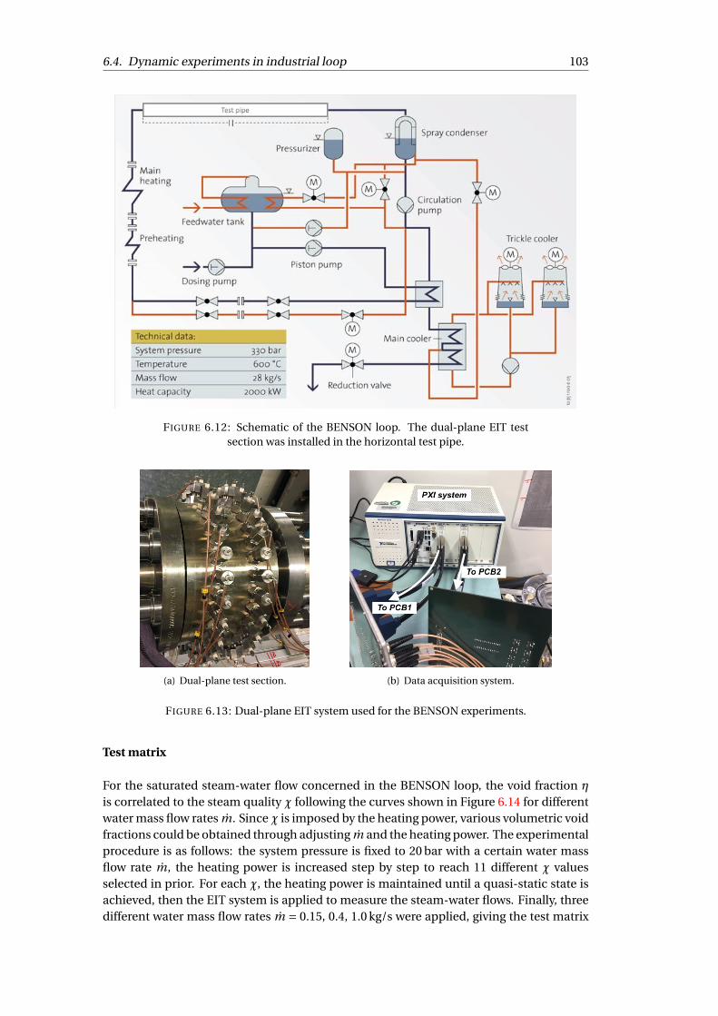
6.4. Dynamic experiments in industrial loop 103
FIGURE 6.12: Schematic of the BENSON loop. The dual-plane EIT testsection was installed in the horizontal test pipe.
(a) Dual-plane test section. (b) Data acquisition system.
FIGURE 6.13: Dual-plane EIT system used for the BENSON experiments.
Test matrix
For the saturated steam-water flow concerned in the BENSON loop, the void fraction ¥
is correlated to the steam quality ¬ following the curves shown in Figure 6.14 for differentwater mass flow rates m. Since ¬ is imposed by the heating power, various volumetric voidfractions could be obtained through adjusting m and the heating power. The experimentalprocedure is as follows: the system pressure is fixed to 20 bar with a certain water massflow rate m, the heating power is increased step by step to reach 11 different ¬ valuesselected in prior. For each ¬, the heating power is maintained until a quasi-static state isachieved, then the EIT system is applied to measure the steam-water flows. Finally, threedifferent water mass flow rates m = 0.15, 0.4, 1.0 kg/s were applied, giving the test matrix

104 Chapter 6. Dynamic two-phase flow experiments
as in Table 6.1, a total of 33 experimental series were conducted, with 3000 frames of imagetaken for each experiment.
FIGURE 6.14: Correlation between the void fraction and the steam qualityat different water mass flow rates.
TABLE 6.1: Test matrix of the experiments in the BENSON loop.
Pressure (bar) 20Mass flow rate (kg/s) m 0.15, 0.4, 1.0Steam quality (%) ¬ 3, 6, 10, 15, 20, 25, 30, 40, 50, 60, 70
6.4.2 Result analysis
During the experiments, the online display of the EIT system gave very poor image re-constructions, the phase distribution could hardly be identified. Possible reasons are dis-cussed in this section, through analyzing the measurement data and assessing the perfor-mance of the EIT system under complex environment, also some perspectives for furtherexperiments are given. In the following analysis, only the data from the second electrodeplane is considered, the analyzed results are compared to that of the ProME-T system un-der laboratory environment with ES2 electrodes (of size 5 mm£4 mm), as they have sim-ilar ratios between the circumferential width occupied by the electrodes and the internalcircumference of the test section.
Noise analysis
In the noise analysis presented in Section 3.3.3, the spectrums of the high and low am-plitude measurements are analyzed in frequency domain, indicating possible origins ofnoises. The SNR and RE are proposed to represent the noise resistance of the system. Thesame analysis has been carried out for the experiments in the BENSON loop.
Figure 6.15 shows the spectrums of the measurement signals at high and low amplitudes,respectively. In the figures, the first peak value at 5 kHz is the fundamental signal, the restare noise. Comparing to the spectrums in laboratory environment shown in Figure 3.10,

6.4. Dynamic experiments in industrial loop 105
it is found that the background noises are almost one order higher for both signals, more-over, there are noises at all frequencies varying with the fundamental amplitudes, whilein Figure 3.10 only the higher-order harmonics vary in such way. From these analysis, thepossible origins of the noises include: 1) the electro-magnetic field caused by the heatingcoils with high power capacity; 2) the vibration of the data acquisition system along withthe platform induced by the circulating pump; 3) other experimental facilities in the samebuilding with the BENSON loop.
(a) High amplitude measurement. (b) Low amplitude measurement.
FIGURE 6.15: Spectrum analysis of the high and low amplitude measure-ments during the BENSON experiments.
The SNR is computed taking the energy of the fundamental signal over the total energy.Figure 6.16 plots the SNR versus the signal amplitude at each measurement channel dur-ing the BENSON experiments, comparing to that of the ProME-T system with ES2 elec-trodes under laboratory environment. As we can see, for the signals with comparativeamplitudes, the SNR in BENSON is significantly higher than in LTHC, yet there are signalswith extremely low amplitudes.
FIGURE 6.16: The Signal to Noise Ratio (SNR) of the system in the BEN-SON loop comparing to that in laboratory environment.

106 Chapter 6. Dynamic two-phase flow experiments
The relative errors RE of repeating measurements have been assessed with nc = 100 con-secutive frames measured at the reference case with homogeneous water filling the pipeline.Five different cases are studied with different configurations listed in Table 6.2, e.g. thenumber of period per excitation pattern Np , the conductivity of water æ0, the excitationamplitudes V0, and whether the heating system is working or not. The RE of case no.2 isplotted versus the signal measurment as in Figure 6.17, in comparison with that of ES2in LTHC. As we can see, for the measurements at comparable amplitudes, the RE for theBENSON loop are considerably lower than that in LTHC in most cases.
FIGURE 6.17: Relative errors of repeating measurements at 50 kHz excita-tion frequency for the BENSON and ES2 in LTHC.
TABLE 6.2: Mean relative error RE for various EIT configurations.
Case no. Np æ0 (µS/cm) V0 (V) Heat RE (dB)
1 1 70 1 heating 18.92 2 70 1 heating 19.53 1 220 1 heating 29.34 1 220 1 no heating 34.95 1 220 3 heating 38.9
The mean relative errors RE of various cases are listed in Table 6.2. It seems that RE in-creases with æ0 and V0, due to the higher measurement amplitudes associated. While theinfluences of transient multiplexing are negligible as the RE with Np = 1 and Np = 2 arecomparable. Furthermore, the RE increases when the heating system is stoped, indicatingthe effects of the electro-magnetic field caused by the heating system. As a conclusion,the mean relative error RE of the EIT system during the BENSON experiments is low forall cases, which explains the poor image reconstructions.
Nevertheless, the eigenvalue based methodology proposed in current thesis study allowsto estimate the phase fraction from boundary measurement without performing imagereconstruction. Specifically for stratified configuration, the phase interface may be iden-tified directly by the indices of the normalized impedance matrix NIM, see Figure 4.3(a)

6.4. Dynamic experiments in industrial loop 107
for the NIM of a simulated stratified configuration with a void fraction of 0.09. The mea-surements over the electrodes uncovered by water would be nearly zero, giving high bulkimpedances. The entries of the low amplitudes in the center of the NIM indicate the in-dices of electrodes uncovered by water, see Figure 6.18 for the NIM of a measured frameunder the conditions m = 0.4 and ¬= 15%, the corresponding void fraction is ¥= 0.52.
FIGURE 6.18: Identifying the water level from the indices of the normal-ized impedance matrix, void fraction ¥= 0.52.
Error analysis and perspectives
In this section, the dual-plane EIT system is assessed by the experiments in the BENSONloop, in terms of noise analysis and features extraction. Overall, the EIT measurementsare too noisy to give meaningful image reconstruction. The possible reasons are: i) thelow measurement signals caused by a low water conductivity and a large pipe diameter;ii) a significantly high noise level comparing to the laboratory environment. Nevertheless,the indices of the normalized impedance matrix may give an indication of the water level.
The perspectives are as follows:
• Reducing the noise level, possible ways include: i) using a Faraday cage to enclosethe data acquisition system; ii) keeping a large distance between the system and theheating coils; iii) increasing the excitation amplitude to have stronger measurementsignals; iv) reducing the vibration of the data acquisition system, insuring a robustcontact of the BNC connector on the board.
• Image reconstruction with EIT measurements from a subset of electrodes.
• Analyzing the effects of the grounded pipe on the measurements. The measure-ment amplitudes may be reduced because of the current leakages from the excita-tion electrodes to the grounded pipe.


109
Chapter 7
Conclusion
Conclusion and discussion
The present Ph.D thesis work demonstrates a comprehensive EIT-based measurementmode for dynamic two-phase flow measurements, with emphasis on the image recon-struction methods and a novel eigenvalue-based approach for flow features extraction,i.e. flow imaging, void fraction estimation, and flow regime identification.
The full-scan excitation strategy considered in the present work sheds new light in theresearches of EIT, where the adjacent strategy is commonly applied. Traversing all inde-pendent pairs of electrodes possible for boundary excitations, full-scan strategy produceshighly redundant measurement data containing that of the adjacent and opposite strate-gies, among others. On one hand, the large number of excitation patterns requires a heavyeffort for multiplexing hence reducing the frame rate. On the other hand, the redundantmeasurements improve the robustness of the system to noise and the overall sensitivity inthe sensing domain, also the sensitivity distribution is more homogeneous comparing tothat of the adjacent strategy. The preeminence of the full-scan and trigonometric strate-gies are evidenced through image reconstructions of several simulation cases and staticexperiments, they give a better geometrical reconstruction of the object(s) and a sharperconductivity contrast compared to the adjacent and opposite strategies. Moreover, the re-dundant measurements allow alternative approaches for void fraction estimation of two-phase flow other than the image reconstruction, namely the eigenvalue-based approach.
The NtD map defined on EIT forward problem and the Neumann boundary conditionsstimulate the idea of impedance matrix, which can be considered as a discrete represen-tation of the NtD map from certain current excitations to corresponding boundary mea-surements. The impedance matrix contains the complete information of phase distribu-tion, its eigenvalues are directly correlated to the phase fraction, allowing an eigenvalue-based methodology for phase fraction estimation. Different correlations are establishedfor three phase distribution patterns through numerical simulations, the reliability of theproposed approach is highlighted by static experiments. A higher estimation accuracyis expected by incorporating a priori knowledge on phase distribution pattern, e.g. thenumber and location of the bubbles. Additionally, it underlines the need for an in-depthmathematical analysis of the relation between the phase distribution and the eigenvaluesof the impedance matrix, such an analysis would allow to determine which informationcan be retrieved from such a matrix and which metrics are suitable to do so. Lastly and asin Bellis et al. (2012), this methodology can be used to devise an initial guess for iterativeimage reconstruction algorithms thereby improving their convergence.

110 Chapter 7. Conclusion
Two-phase flows feature a quickly evolving phase distribution and a high conductivitycontrast between the phases, raising additional requirements for image reconstructions.Various reconstruction methods, e.g. the least-squares methods with different regulariza-tions, GREIT, factorization method, MUSIC algorithm, and topological sensitivity method,are reviewed and discussed in terms of two-phase flow imaging. Their implementationprocedures are demonstrated by numerical simulations, finally the one-step 2.5D recon-struction, 2D iterative methods with Tikhonov and TV regularizations, and GREIT are se-lected for further studies with experimental data. Although the MUSIC algorithm seemsappealing considering the high efficiency in locating inhomogeneities, some improve-ments should be made to enhance its performance with noisy data. Benchmark recon-structions are made applying the four selected methods to several static experiments withthe ES1 and ES2 electrodes. Results show that the quality of the reconstructed images aresignificantly affected by the length of the electrodes, generally, the 2.5D and GREIT meth-ods give satisfactory image reconstructions for both the ES1 and ES2 electrodes, while the2D iterative methods are not promising for ES2 electrodes. Considering the performanceanalysis of the ProME-T system with two sets of electrodes and the numerical simulationsof 3D effect, longer electrodes (with a larger surface area) are envisaged to give a higheroverall measurement amplitude and a more homogeneous sensitivity distribution in thesensing domain, hence a better image reconstruction. On the contrary, the axial sens-ing domain associated with longer electrodes would extend further, being less sensitive tosmall local changes in dynamic flows. A compromise should be made between the twoaspects.
Dynamic two-phase flow experiments have been conducted in the processing lab of Uni-versity College of South-East Norway in collaboration with Professor Mylvaganam. De-veloped horizontal air-water flows at ambient temperature and pressure were measuredusing the ultra-high speed ONE-SHOT system developed in LTHC. The transverse cross-sectional images are reconstructed from the EIT measurements using 2.5D method, theaxially stacked EIT tomograms provide valuable information about the flows: the flow pat-tern could be identified by visual inspection, the volume averaged void fraction could beestimated from the eigenvalues correlation method and conductivity threshold methodseparately. The high frame rate of EIT allows a higher time resolution than GRM, revealingthe different characters at the front of a plug/slug. The reliability of the eigenvalue-basedapproach is again highlighted by dynamic experimental results, the volume averaged voidfraction is well correlated to the leading eigenvalue of the averaged normalized impedancematrix, except for some cases where transition between stratified smooth and wavy flowsoccurs. Applying correlation techniques with the eigenvalues of the EIT impedance matrixin vertical two-phase flows would lead to interesting results with respect to annular andstratified flows, as most of the peripheral electrodes will be in contact with the conduct-ing water medium. Additionally, efforts have been made to apply GREIT method to themeasurement data, the result is not promising because of the relatively high noise levelin dynamic experiments and the measurement errors induced by the multiple excitationfrequencies used for FDM in the ONE-SHOT system.
Another set of dynamic experiments were performed in the BENSON loop during my visitat Framatome GmbH, Germany, horizontal steam-water flows at high temperature highpressure were measured at various steam qualities. The designed dual-plane test sec-tion is proved to sustain the harsh flows successfully, however, the image reconstructionsare too noisy to retrieve meaningful information. The measured signals are analyzed infrequency domain, giving possible origins of the measurment noises, including: i) the

Chapter 7. Conclusion 111
electro-magnetic field generated by the high capacity electrical heating coils; ii) the mal-function of the BNC connectors induced by the vibration of the system. Future experi-ments with proper electro-magnetic shielding and anti-vibration practice are expected togive better results.
Perspective
Insensitive researches on electrical tomography are ongoing for the development of in-novative instrumentations, there are several aspects to be studied in-depth which bringsprospects toward the long-term goal of applying EIT for flow measurements under harshenvironments.
Considering that the number of independent measurements of an EIT system is restrictedby the number of electrodes, a straightforward way to improve the spatial resolution isemploying more electrodes, especially, the current hardwares for data acquisition andmanipulation are sufficient to handle 32 even 64 electrodes. Currently two test sectionsare available in LTHC, one with a single plane of 32 electrodes, another one with threeplanes of 16 electrodes. It is feasible and promising to upgrade the ProME-T system to a32 channels EIT system, allowing different excitation and measurement strategies. Specif-ically for the multi-plane test section, two different strategies can be applied with properupdates of the acquisition codes and PCB, i.e. i) independent working strategy where twoelectrode planes work independently at different excitation frequencies, cross-plane mea-surements can be obtained discriminating the measured signals through FFT, making fre-quency difference reconstruction possible, which can circumvent the need of a referencemeasurement (Malone et al., 2013); ii) adjoint working strategy where cross-plane excita-tions are applied to improve the sensitivity in the center of the domain, several researcheshave proved the superiority of cross-plane excitations and measurements for 3D imagereconstructions (Wagenaar and Adler, 2016; Grychtol et al., 2019).
In the light of present thesis work, the preeminence of the full-scan excitation strategy isevidenced comparing to the adjacent one, however, it is somehow time assuming to tra-verse all independent pairs of electrodes for full-scan excitations, especially when thereare large number of electrodes on multiple planes for cross-plane excitations. Other strate-gies, for example the over-2 or -3 strategies with a separation of 2 or 3 electrodes betweenthe source and drain (Alme and Mylvaganam, 2007), may have comparably good perfor-mances as the full-scan while requiring less redundant excitations, hence a higher framerate. Moreover, the weighting of adjacent excitation is reduced in over-2 or -3 strategiescomparing to the full-scan, which may grant a more homogeneous sensitivity distributionand reduce the ill-posedness of EIT inverse problem.
Multi-modality sensors are attracting more attentions and of interest for continuationof the present work, they can discriminate different materials with similar conductiv-ity or permittivity, or improve the system performance. For example, the dual-modalityEIT/ECT sensor can discriminate three phases through conductivity and permittivity re-constructions, allowing wide applications in oil extraction (Wang et al., 2017). The EIT andultrasonic sensors can perform image reconstructions on the same mesh model, since achange in conductivity is usually accompanied by a change in acoustic impedance, dual-modality EIT and ultrasonic sensors may have a better performance in terms of imagequality and robustness to noise (Liang et al., 2019).

112 Chapter 7. Conclusion
In terms of image reconstruction, the present work puts a lot efforts on the feasible recon-struction methods for two-phase flow imaging. The GREIT method seems very promis-ing considering the computation efficiency and image quality for both sets of electrodes.Further investigations should be performed with measurment data from dynamic exper-iments, also the method itself maybe modified specifically for the applications in two-phase flow imaging. The MUSIC algorithm has been studied preliminarily in the presentwork, considering point electrodes on the boundary with gap electrode model and nu-merical simulation data. For practical implementation, electrodes with physical size andcomplete electrode model should be considered, by which its performance with noisydata may be improved. Further, the position and number of the inclusions provided bythe MUSIC algorithm may be incorporated in iterative image reconstruction methods asan initial guess to improve their convergences.
Considering the applications in industrial flow measurements, the background noise andcurrent leakage from the electrodes to the conductive pipelines are challenging. Increas-ing the electrode length may strengthen the measurement signals, while it also enlargesthe sensing volume and reduces the sensitivity to local flow changes, a compromise shouldbe made between the two aspects. Besides, in some cases a reference measurement withhomogeneous medium filling the pipeline may be not feasible, the temperature changesduring the experiments may induce conductivity variations and distort the reconstructedimages. It is difficult and expensive to acquire the real-time conductivity, a temperaturecoefficient can be considered to bypass this problem (Jia et al., 2015). That is, the mediumin the loop can be sampled before the experiments, the conductivity is measured at a set oftemperatures to estimate the temperature coefficient. The reference boundary measure-ments at various temperatures can be obtained given the real-time temperature and thetemperature coefficient. The influences of changing temperature on the reconstructedimages are excluded, only the phase change is considered.

113
Appendix A
Dual-plane test section design forPKL
Figure A.1 shows the final design of the dual-plane test section for the PKL facility, it hasan inner diameter of 128.2 mm and a length of 170 mm. To withstand the high tempera-ture high pressure flows inside the pipe, the test section is made of stainless steel, but itsinner surface is coated to be electrically insulating except for the surfaces of electrodes.The test section has 32 plate-like electrodes on each plane, the connectors of the elec-trodes are designed specifically to avoid water leakage under harsh environment. Thedesign of the electrodes is shown in Figure A.2, the electrode surface is a rectangular ofsize 15 mm£11.5 mm, the long bar passes through the pipe wall and carries the signalsbetween the electrode surface and the PCB.
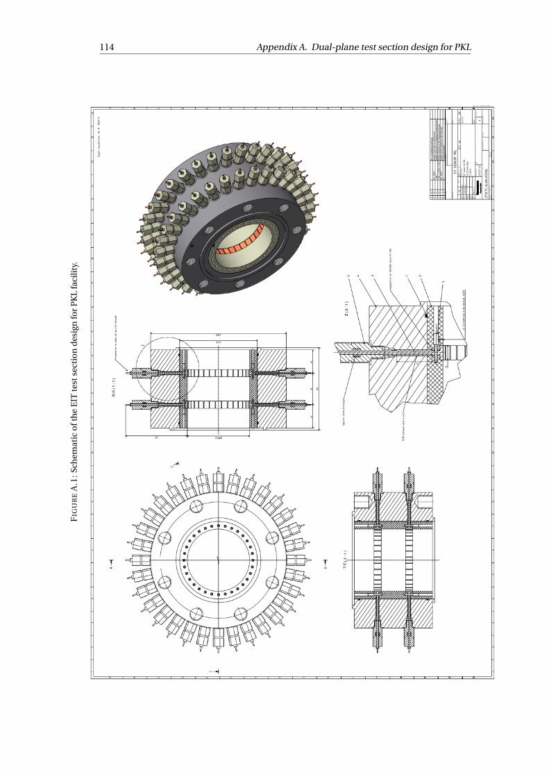
114 Appendix A. Dual-plane test section design for PKL
FIG
UR
EA
.1:S
chem
atic
ofth
eE
ITte
stse
ctio
nde
sign
for
PKL
faci
lity.

Appendix A. Dual-plane test section design for PKL 115F
IGU
RE
A.2
:Sch
emat
icof
the
elec
trod
esu
sed
inth
eE
ITte
stse
ctio
nfo
rPK
Lfa
cilit
y.
����
�������
���
����
������
��
$%
��
��
��
��
��
��
��
( ' &)) ' % $( &
$87(85
9(5,)�
$335�
)$%�
48$
/�
6$8)�,1
',&$7,2
1�&2175$,5(�
/(6�&27(6�62
17�(1
�0,//,0(75(6
(7$7�'(�685)$&(�
72/(5$
1&(6�
���/,1
($,5(6�
���$1*8/$,5(6�
),1,7,21�
&$66(5�/(6
$1*/(6�9,)6
120
6,*1$785(
'$7(
0$7(5,$8�
1(�3$
6�&+$
1*(5�/(&+(
//(
5(9,6,21
7,75(�
1R��'(�3/$1
(&+(
//(����
)(8,//(���685��
$�
0$66(��
HOHF
BGHVLJQ


117
Appendix B
EIT and GRM tomograms forexperiments in USN
This Appendix shows the EIT and GRM tomograms for some selected experimental seriesconducted in the horizontal flow loop of USN. Each experimental series corresponds toa pair of water and air flow rates, the experiment numbering and associated flow regimeare shown in Figure 6.7. A total of 10 experimental series are chosen, two for each flowregime, including: test 03 and 09 for slug flow, test 01 and 13 for plug flow, test 39 and 74for stratified smooth flow, test 44 and 71 for stratified wavy flow, test 66 and 73 for annularflow.
In both EIT and GRM tomograms, the abscissa represents the measurement time, 30 sec-onds of measurements are taken for both tomograms. The EIT tomograms plot the differ-ence conductivity ¢æ between water and air, therefore, the red color indicates the water,the blue for air. Similar in the GRM tomograms, the red color represents the water.
EIT tomograms on the top, GRM tomograms on the bottom
Continued on next page

118 Appendix B. EIT and GRM tomograms for experiments in USN
Continued on next page

Appendix B. EIT and GRM tomograms for experiments in USN 119


121
Bibliography
A. Adler and R. Guardo. Electrical impedance tomography: regularized imaging and con-trast detection. IEEE transactions on medical imaging, 15(2):170–179, 1996.
A. Adler and W. R. Lionheart. Uses and abuses of EIDORS: an extensible software base forEIT. Physiological measurement, 27(5):S25, 2006.
A. Adler, J. H. Arnold, R. Bayford, A. Borsic, B. Brown, P. Dixon, T. J. Faes, I. Frerichs,H. Gagnon, Y. Gärber, et al. GREIT: a unified approach to 2D linear EIT reconstructionof lung images. Physiological measurement, 30(6):S35, 2009.
A. Adler, P. O. Gaggero, and Y. Maimaitijiang. Adjacent stimulation and measurement pat-terns considered harmful. Physiological measurement, 32(7):731, 2011.
A. Adler, A. Boyle, and W. R. Lionheart. Efficient computations of the Jacobian matrix usingdifferent approaches are equivalent. ELECTRICAL IMPEDANCE TOMOGRAPHY!, 21:75,2017.
S. Aguiar Santos, A. Robens, A. Boehm, S. Leonhardt, and D. Teichmann. System descrip-tion and first application of an FPGA-based simultaneous multi-frequency electricalimpedance tomography. Sensors, 16(8):1158, 2016.
W. H. Ahmed and B. I. Ismail. Innovative techniques for two-phase flow measurements.Recent Patents on Electrical & Electronic Engineering (Formerly Recent Patents on Elec-trical Engineering), 1(1):1–13, 2008.
K. J. Alme and S. Mylvaganam. Comparison of different measurement protocols in electri-cal capacitance tomography using simulations. IEEE Transactions on Instrumentationand Measurement, 56(6):2119–2130, 2007.
G. Bal and K. Ren. On multi-spectral quantitative photo-acoustic tomography in diffusiveregime. Inverse Problems, 28(2):025010, 2012.
G. Bal and G. Uhlmann. Inverse diffusion theory of photoacoustics. Inverse Problems, 26(8):085010, 2010.
D. C. Barber and B. H. Brown. Applied potential tomography. Journal of Physics E: ScientificInstruments, 17(9):723, 1984.
C. Bellis, A. Constantinescu, T. Coquet, T. Jaravel, and A. Lechleiter. A non-iterative sam-pling approach using noise subspace projection for EIT. Inverse Problems, 28(7):075015,2012.
M. Bonnet. Higher-order topological sensitivity for 2-D potential problems. Applicationto fast identification of inclusions. International Journal of Solids and Structures, 46(11-12):2275–2292, 2009.
M. Bonnet and F. Cakoni. Analysis of topological derivative as a tool for qualitative identi-fication. Inverse Problems, 2019.

122 BIBLIOGRAPHY
L. Borcea. Electrical impedance tomography. Inverse problems, 18(6):R99, 2002.
A. Borsic, B. M. Graham, A. Adler, and W. R. Lionheart. In vivo impedance imaging withtotal variation regularization. IEEE transactions on medical imaging, 29(1):44–54, 2009.
A. Boyle and A. Adler. The impact of electrode area, contact impedance and boundaryshape on EIT images. Physiological measurement, 32(7):745, 2011.
W. Breckon and M. Pidcock. Some mathematical aspects of electrical impedance tomogra-phy. In Mathematics and computer science in medical imaging, pages 351–362. Springer,1988.
W. R. Breckon. Image reconstruction in electrical impedance tomography. PhD thesis, Ox-ford Polytechnic, 1990.
J. Brewer. Kronecker products and matrix calculus in system theory. IEEE Transactions oncircuits and systems, 25(9):772–781, 1978.
M. Brühl. Explicit Characterization of Inclusions in Electrical Impedance Tomography.Siam Journal on Mathematical Analysis - SIAM J MATH ANAL, 32, 02 2001. doi: 10.1137/S003614100036656X.
M. Brühl and M. Hanke. Numerical implementation of two noniterative methods for lo-cating inclusions by impedance tomography. Inverse Problems, 16(4):1029, 2000.
A. P. Calderón. On an inverse boundary value problem. Computational & Applied Mathe-matics, 25(2-3):133–138, 2006.
S. Ceccio and D. George. A review of electrical impedance techniques for the measurementof multiphase flows. Journal of fluids engineering, 118(2):391–399, 1996.
Y. Chen, W. P. Jepson, and H. J. Chen. Effects of multiphase flow on corrosion inhibitor.CORROSION 99, 1999.
M. Cheney and D. Isaacson. Distinguishability in impedance imaging. IEEE Transactionson Biomedical Engineering, 39(8):852–860, 1992.
M. Cheney, D. Isaacson, J. C. Newell, S. Simske, and J. Goble. NOSER: An algorithm forsolving the inverse conductivity problem. International Journal of Imaging systems andtechnology, 2(2):66–75, 1990.
M. Cheney, D. Isaacson, and J. C. Newell. Electrical impedance tomography. SIAM review,41(1):85–101, 1999.
K.-S. Cheng, D. Isaacson, J. Newell, and D. G. Gisser. Electrode models for electric currentcomputed tomography. IEEE Transactions on Biomedical Engineering, 36(9):918–924,1989.
E. T. Chung, T. F. Chan, and X.-C. Tai. Electrical impedance tomography using level setrepresentation and total variational regularization. Journal of Computational Physics,205(1):357–372, 2005.
R. D. Cook, G. J. Saulnier, D. G. Gisser, J. C. Goble, J. Newell, and D. Isaacson. ACT3: A high-speed, high-precision electrical impedance tomograph. IEEE Transactions on Biomedi-cal Engineering, 41(8):713–722, 1994.
N. cRIO. DEVICE SPECIFICATIONS NI cRIO-9039: Embedded CompactRIO Controller withReal-Time Processor and Reconfigurable FPGA. National Instrument, 2018.

BIBLIOGRAPHY 123
C. Dang, M. Darnajou, G. Ricciardi, A. Beisiegel, S. Bourennane, and C. Bellis. Performanceanalysis of an electrical impedance tomography sensor with two sets of electrodes ofdifferent sizes. Proc. WCIPT-9 (Bath, UK), 2018a.
C. Dang, M. Darnajou, G. Ricciardi, L. Rossi, S. Bourennane, C. Bellis, and H. Schmidt.Two-phase flow void fraction estimation from the raw data of electrical impedance to-mography sensor. Proc. ICAPP (Juan-les-Pins, France), 2018b.
C. Dang, M. Darnajou, C. Bellis, G. Ricciardi, H. Schmidt, and S. Bourennane. Numericaland experimental analysis of the correlation between EIT data eigenvalues and two-phase flow phase fraction. Measurement Science and Technology, 31(1):015302, 2019a.
C. Dang, M. Darnajou, G. Ricciardi, L. Rossi, S. Bourennane, C. Bellis, and H. Schmidt.Spectral And Eigenvalues Analysis of Electrical Impedance Tomography Data For FlowRegime Identification. Proc. SWINTH (Livorno, Italy), 2019b.
C. Dang, C. Bellis, M. Darnajou, G. Ricciardi, S. Mylvaganam, and S. Bourennane. PracticalComparisons of EIT Excitation Protocols with Applications in High Contrast Imaging.Instrumentation Science and Technology, Submitted.
C. Dang, M. Darnajou, C. Bellis, G. Ricciardi, S. Mylvaganam, and S. Bourennane. Im-proving EIT-based visualizations of two-phase flows using an eigenvalue correlationmethod. IEEE Transactions on Instrumentation and Measurement, Submitted.
M. Darnajou, C. Dang, G. Ricciardi, S. Bourennane, C. Bellis, and H. Schmidt. The De-sign of Electrical Impedance Tomography Detectors in Nuclear Industry. Proc. WCIPT-9(Bath, UK), 2018.
M. Darnajou, A. Dupré, C. Dang, G. Ricciardi, S. Bourennane, and C. Bellis. On the Imple-mentation of Simultaneous Multi-Frequency Excitations and Measurements for Electri-cal Impedance Tomography. Sensors, 19(17):3679, 2019.
M. Darnajou, A. Dupré, C. Dang, G. Ricciardi, S. Bourennane, C. Bellis, and S. Mylva-ganam. High Speed EIT with Multifrequency Excitation using FPGA and Response Anal-ysis using FDM. IEEE Sensors Journal, 2020.
E. Demidenko, A. Hartov, N. Soni, and K. D. Paulsen. On optimal current patterns forelectrical impedance tomography. IEEE Transactions on Biomedical Engineering, 52(2):238–248, 2005.
X. Deng, F. Dong, L. Xu, X. Liu, and L. Xu. The design of a dual-plane ert system forcross correlation measurement of bubbly gas/liquid pipe flow. Measurement Scienceand Technology, 12(8):1024, 2001.
F. Dickin and M. Wang. Electrical resistance tomography for process applications. Mea-surement Science and Technology, 7(3):247, 1996.
N. Dominguez and V. Gibiat. Non-destructive imaging using the time domain topologicalenergy method. Ultrasonics, 50(3):367–372, 2010.
F. Dong, Y. Xu, L. Hua, and H. Wang. Two methods for measurement of gas-liquid flows invertical upward pipe using dual-plane ERT system. IEEE Transactions on Instrumenta-tion and Measurement, 55(5):1576–1586, 2006.
A. Dupré. Electrical impedance tomography for void fraction measurements of harsh two-phase flows: prototype development and reconstruction techniques. PhD thesis, EcoleCentrale Marseille, 2017.

124 BIBLIOGRAPHY
A. Dupré and S. Mylvaganam. A Simultaneous and Continuous Excitation Method forHigh-Speed Electrical Impedance Tomography with Reduced Transients and Noise Sen-sitivity. Sensors, 18(4):1013, 2018.
A. Dupré, G. Ricciardi, and S. Bourennane. Novel Approach for Analysis and Designof High-Speed Electrical Impedance Tomographic System for Void Fraction Measure-ments in Fast Two-Phase Flows. IEEE Sensors Journal, 17(14):4472–4482, 2017a.
A. Dupré, G. Ricciardi, S. Bourennane, and S. Mylvaganam. Electrical Capacitance-BasedFlow Regimes Identification - Multiphase Experiments and Sensor Modeling. IEEE Sen-sors Journal, 17(24):8117–8128, 2017b.
J. Enrique Julia, W. K. Harteveld, R. F. Mudde, and H. E. Van den Akker. On the accuracy ofthe void fraction measurements using optical probes in bubbly flows. Review of scientificinstruments, 76(3):035103, 2005.
H. A. Eschenauer, V. V. Kobelev, and A. Schumacher. Bubble method for topology andshape optimization of structures. Structural optimization, 8(1):42–51, 1994.
W. Fang and E. Cumberbatch. Matrix properties of data from electrical capacitance to-mography. Journal of engineering mathematics, 51(2):127–146, 2005.
L. F. Fuks, M. Cheney, D. Isaacson, D. G. Gisser, and J. Newell. Detection and imaging ofelectric conductivity and permittivity at low frequency. IEEE Transactions on BiomedicalEngineering, 38(11):1106–1110, 1991.
J. Gamio, J. Castro, L. Rivera, J. Alamilla, F. Garcia-Nocetti, and L. Aguilar. Visualisation ofgas–oil two-phase flows in pressurised pipes using electrical capacitance tomography.Flow Measurement and Instrumentation, 16(2-3):129–134, 2005.
D. George, J. Torczynski, K. Shollenberger, T. O’Hern, and S. Ceccio. Validation ofelectrical-impedance tomography for measurements of material distribution in two-phase flows. International Journal of Multiphase Flow, 26(4):549–581, 2000.
D. Gisser, D. Isaacson, and J. Newell. Current topics in impedance imaging. ClinicalPhysics and Physiological Measurement, 8(4A):39, 1987.
D. Gisser, D. Isaacson, and J. Newell. Electric current computed tomography and eigen-values. SIAM Journal on Applied Mathematics, 50(6):1623–1634, 1990.
C. Goh, A. Ruzairi, F. Hafiz, and Z. Tee. Ultrasonic tomography system for flow monitoring:A review. IEEE Sensors Journal, 17(17):5382–5390, 2017.
B. Graham and A. Adler. Objective selection of hyperparameter for EIT. Physiologicalmeasurement, 27(5):S65, 2006.
B. Graham and A. Adler. Electrode placement configurations for 3D EIT. Physiologicalmeasurement, 28(7):S29, 2007.
B. Grychtol, B. Müller, and A. Adler. 3D EIT image reconstruction with GREIT. Physiologi-cal measurement, 37(6):785, 2016.
B. Grychtol, J. P. Schramel, F. Braun, T. Riedel, U. Auer, M. Mosing, C. Braun, A. D. Wald-mann, S. H. Böhm, and A. Adler. Thoracic EIT in 3D: experiences and recommendations.Physiological measurement, 40(7):074006, 2019.
B. B. Guzina and M. Bonnet. Small-inclusion asymptotic of misfit functionals for inverseproblems in acoustics. Inverse Problems, 22(5):1761, 2006.

BIBLIOGRAPHY 125
M. Hanke and M. Brühl. Recent progress in electrical impedance tomography. InverseProblems, 19(6):S65, 2003.
Z. Hao, S. Yue, B. Sun, and H. Wang. Optimal distance of multi-plane sensor in three-dimensional electrical impedance tomography. Computer Assisted Surgery, 22(sup1):326–338, 2017.
F. Hecht. New development in FreeFem++. J. Numer. Math., 20(3-4):251–265, 2012. ISSN1570-2820. URL https://freefem.org/.
T. J. Heindel. A review of X-ray flow visualization with applications to multiphase flows.Journal of Fluids Engineering, 133(7):074001, 2011.
D. Holder. Electrical impedance tomography: methods, history and applications. CRCPress, 2004.
P. Hua, J. Webster, and W. Tompkins. A regularised electrical impedance tomographyreconstruction algorithm. Clinical Physics and Physiological Measurement, 9(4A):137,1988.
Z. Huang, B. Wang, and H. Li. Application of electrical capacitance tomography to thevoid fraction measurement of two-phase flow. IEEE Transactions on Instrumentationand Measurement, 52(1):7–12, 2003.
D. Isaacson, J. L. Mueller, J. C. Newell, and S. Siltanen. Reconstructions of chest phan-toms by the D-bar method for electrical impedance tomography. IEEE Transactions onMedical Imaging, 23(7):821–828, 2004.
J. Jia, M. Wang, Y. Faraj, and Q. Wang. Online conductivity calibration methods for EITgas/oil in water flow measurement. Flow Measurement and Instrumentation, 46:213–217, 2015.
J. Jia, H. Wang, and D. Millington. Electrical resistance tomography sensor for highlyconductive oil-water two-phase flow measurement. IEEE Sensors Journal, 17(24):8224–8233, 2017.
R. Johansen, T. Østby, A. Dupre, and S. Mylvaganam. LONG SHORT-TERM MEMORY NEU-RAL NETWORKS FOR FLOW REGIME IDENTIFICATION USING ECT. 09 2018.
O. C. Jones Jr and J.-M. Delhaye. Transient and statistical measurement techniques fortwo-phase flows: a critical review. International Journal of Multiphase Flow, 3(2):89–116, 1976.
P. Kauppinen, J. Hyttinen, and J. Malmivuo. Sensitivity distribution visualizations ofimpedance tomography measurement strategies. International Journal of Bioelectro-magnetism, 8(1):1–9, 2006.
M. T. M. Khairi, S. Ibrahim, M. A. M. Yunus, M. Faramarzi, G. P. Sean, J. Pusppanathan, andA. Abid. Ultrasound computed tomography for material inspection: Principles, designand applications. Measurement, 146:490–523, 2019.
M. C. Kim, S. Kim, K. Y. Kim, and Y. J. Lee. Regularization methods in electrical impedancetomography technique for the two-phase flow visualization. International communica-tions in heat and mass transfer, 28(6):773–782, 2001.
A. Kirsch. Characterization of the shape of a scattering obstacle using the spectral data ofthe far field operator. Inverse problems, 14(6):1489, 1998.

126 BIBLIOGRAPHY
R. V. Kohn and A. McKenney. Numerical implementation of a variational method for elec-trical impedance tomography. Inverse Problems, 6(3):389, 1990.
V. Kolehmainen, S. Siltanen, S. Järvenpää, J. P. Kaipio, P. Koistinen, M. Lassas, J. Pirttilä, andE. Somersalo. Statistical inversion for medical x-ray tomography with few radiographs:II. Application to dental radiology. Physics in Medicine & Biology, 48(10):1465, 2003.
C. Kotre. EIT image reconstruction using sensitivity weighted filtered backprojection.Physiological measurement, 15(2A):A125, 1994.
R. Kotze, A. Adler, A. Sutherland, and C. Deba. Evaluation of Electrical Resistance Tomog-raphy imaging algorithms to monitor settling slurry pipe flow. Flow Measurement andInstrumentation, page 101572, 2019.
G. Liang, S. Ren, S. Zhao, and F. Dong. A Lagrange-Newton method for EIT/UT dual-modality image reconstruction. Sensors, 19(9):1966, 2019.
W. R. Lionheart. EIT reconstruction algorithms: pitfalls, challenges and recent develop-ments. Physiological measurement, 25(1):125, 2004.
W. R. Lionheart, J. Kaipio, and C. N. McLeod. Generalized optimal current patterns andelectrical safety in EIT. Physiological measurement, 22(1):85, 2001.
Y. Ma, H. Wang, L.-A. Xu, and C. Jiang. Simulation study of the electrode array used in anERT system. Chemical engineering science, 52(13):2197–2203, 1997.
E. Malone, G. S. dos Santos, D. Holder, and S. Arridge. Multifrequency electricalimpedance tomography using spectral constraints. IEEE transactions on medical imag-ing, 33(2):340–350, 2013.
J. Mandhane, G. Gregory, and K. Aziz. A flow pattern map for gas-liquid flow in horizontalpipes. International Journal of Multiphase Flow, 1(4):537–553, 1974.
R. Mudde. Bubbles in a fluidized bed: A fast X-ray scanner. AIChE journal, 57(10):2684–2690, 2011.
J. L. Mueller and S. Siltanen. Linear and nonlinear inverse problems with practical appli-cations, volume 10. Siam, 2012.
S. Nedeltchev, U. Hampel, and M. Schubert. Investigation of the radial effect on the tran-sition velocities in a bubble column based on the modified Shannon entropy. ChemicalEngineering Research and Design, 115:303–309, 2016.
J. Newell, D. Isaacson, M. Cheney, G. Saulnier, D. Gisser, J. Goble, R. Cook, P. Edic, C. New-ton, and D. Holder. In Vivo impedance images using sinusoidal current patterns. Clin-ical and Physiological Applications of Electrical Impedance Tomography, pages 277–98,1993.
S. Paranjape, S. N. Ritchey, and S. V. Garimella. Electrical impedance-based void fractionmeasurement and flow regime identification in micro-channel flows under adiabaticconditions. International Journal of Multiphase Flow, 42:175–183, 2012.
S. Paras and A. Karabelas. Properties of the liquid layer in horizontal annular flow. Inter-national journal of multiphase flow, 17(4):439–454, 1991.
H. V. Peña and O. Rodriguez. Applications of wire-mesh sensors in multiphase flows. Flowmeasurement and instrumentation, 45:255–273, 2015.

BIBLIOGRAPHY 127
K. Perera, C. Pradeep, S. Mylvaganam, and R. W. Time. Imaging of oil-water flow patternsby electrical capacitance tomography. Flow Measurement and Instrumentation, 56:23–34, 2017.
R. Plonsey and R. Collin. Electrode guarding in electrical impedance measurements ofphysiological systems—a critique. Medical and Biological Engineering and Computing,15(5):519–527, 1977.
N. Polydorides. Image reconstruction algorithms for soft-field tomography. PhD Thesis,UMIST, 2002.
N. Polydorides and W. R. Lionheart. A Matlab toolkit for three-dimensional electricalimpedance tomography: a contribution to the Electrical Impedance and Diffuse Opti-cal Reconstruction Software project. Measurement science and technology, 13(12):1871,2002.
H.-M. Prasser, A. Böttger, and J. Zschau. A new electrode-mesh tomograph for gas–liquidflows. Flow measurement and instrumentation, 9(2):111–119, 1998.
J. Pusppanathan, R. A. Rahim, F. A. Phang, E. J. Mohamad, N. M. N. Ayob, M. H. F. Rahiman,and C. K. Seong. Single-plane dual-modality tomography for multiphase flow imagingby integrating electrical capacitance and ultrasonic sensors. IEEE Sensors Journal, 17(19):6368–6377, 2017.
N. PXIe. DEVICE SPECIFICATIONS NI 6368 X Series Data Acquisition. National Intrusment,2016.
G. Ricciardi, M. Pettigrew, and N. Mureithi. Fluidelastic Instability in a Normal TriangularTube Bundle Subjected to Air-Water Cross-Flow. Journal of Pressure Vessel Technology,133:9, 10 2011. doi: 10.1115/1.4004562.
L. Rossi, R. De Fayard, and S. Kassab. Measurements using X-ray attenuation vertical dis-tribution of the void fraction for different flow regimes in a horizontal pipe. NuclearEngineering and Design, 336:129–140, 2018.
Y. Ru and S. Mylvaganam. Enhanced flow regime identification with SVM using electri-cal capacitance tomography (ECT) in fluidized beds. 7th World Congress in IndustrialProcess Tomography, pages 809–817, 01 2014.
C. M. Salgado, C. M. Pereira, R. Schirru, and L. E. Brandão. Flow regime identification andvolume fraction prediction in multiphase flows by means of gamma-ray attenuationand artificial neural networks. Progress in Nuclear Energy, 52(6):555–562, 2010.
F. Santosa and M. Vogelius. A backprojection algorithm for electrical impedance imaging.SIAM Journal on Applied Mathematics, 50(1):216–243, 1990.
E. Schleicher, M. Tschofen, R. Kipping, and U. Hampel. Wire-mesh Sensors: Recent De-velopments and Applications. Proc. SWINTH (Livorno, Italy), 2016.
A. Seagar, D. Barber, and B. Brown. Theoretical limits to sensitivity and resolution inimpedance imaging. Clinical Physics and Physiological Measurement, 8(4A):13, 1987.
M. Sharifi and B. Young. Electrical resistance tomography (ERT) applications to chemicalengineering. Chemical Engineering Research and Design, 91(9):1625–1645, 2013.
E. Somersalo, M. Cheney, and D. Isaacson. Existence and uniqueness for electrode modelsfor electric current computed tomography. SIAM Journal on Applied Mathematics, 52(4):1023–1040, 1992.

128 BIBLIOGRAPHY
D. Stephenson, R. Mann, and T. York. The sensitivity of reconstructed images and pro-cess engineering metrics to key choices in practical electrical impedance tomography.Measurement Science and Technology, 19(9):094013, 2008.
J. Sun and W. Yang. Evaluation of fringe effect of electrical resistance tomography sensor.Measurement, 53:145–160, 2014.
J. Sun and W. Yang. A dual-modality electrical tomography sensor for measurement ofgas–oil–water stratified flows. Measurement, 66:150–160, 2015.
Y. Taitel and A. E. Dukler. A model for predicting flow regime transitions in horizontal andnear horizontal gas-liquid flow. AIChE journal, 22(1):47–55, 1976.
Y. Taitel, D. Bornea, and A. Dukler. Modelling flow pattern transitions for steady upwardgas-liquid flow in vertical tubes. AIChE Journal, 26(3):345–354, 1980.
C. Tan, F. Dong, and M. Wu. Identification of gas/liquid two-phase flow regime throughERT-based measurement and feature extraction. Flow Measurement and Instrumenta-tion, 18(5-6):255–261, 2007.
M. Vauhkonen. Electrical impedance tomography and prior information. PhD thesis, Kuo-pio University, Kuopio, 1997.
J. Wagenaar and A. Adler. Electrical impedance tomography in 3D using two electrodeplanes: characterization and evaluation. Physiological measurement, 37(6):922, 2016.
H. Wang and L. Zhang. Identification of two-phase flow regimes based on support vectormachine and electrical capacitance tomography. Measurement Science and Technology,20(11):114007, 2009.
M. Wang. Electrode models in electrical impedance tomography. Journal of ZhejiangUniversity-SCIENCE A, 6(12):1386–1393, 2005.
Q. Wang, M. Wang, K. Wei, and C. Qiu. Visualization of gas–oil–water flow in horizontalpipeline using dual-modality electrical tomographic systems. IEEE Sensors Journal, 17(24):8146–8156, 2017.
P. Wiedemann, A. Döß, E. Schleicher, and U. Hampel. Fuzzy flow pattern identificationin horizontal air-water two-phase flow based on wire-mesh sensor data. InternationalJournal of Multiphase Flow, 117:153–162, 2019.
J. Wtorek, A. Bujnowski, and H. Sahli. Influence of electrode size on a Jacobian properties.2004.
W. Yan, S. Hong, and R. Chaoshi. Optimum design of electrode structure and parametersin electrical impedance tomography. Physiological measurement, 27(3):291, 2006.
T. J. Yorkey, J. G. Webster, and W. J. Tompkins. Comparing reconstruction algorithms forelectrical impedance tomography. IEEE Transactions on Biomedical Engineering, (11):843–852, 1987.