IMAGE-SPACE SHEET-BUFFERED SPLATTING ON GPU

Sergi Grau and Dani Tost Divisió Informàtica Gràfica

Centre de Recerca de Enginyeria Biomèdica UPC Barcelona (Spain)

ABSTRACT

Image-Space Sheet-Buffered Splatting is a popular high quality volume-rendering technique specially suitable for zoomed views of the data and point-based surface models, that projects the voxels in slabs perpendicular to the viewing direction. Recently, a GPU design of this method has been proposed that considerably accelerates the rendering stage. However, the bottleneck of the method is the computation of the buckets, i.e the structure handling the voxels to be rendered in each slab. This stage of the method is done on the CPU. In this paper, we propose a new design of the method that creates and manages the buckets on the GPU. The proposed method is more than 6.5 times faster than the previous ones.

KEYWORDS

Volume rendering. Splatting. GPU.

1. INTRODUCTION

Splatting was originally proposed as a feed-forward algorithm for voxel-based volume datasets [17]. Recently, it has gained popularity in being applied to point-based surface models [1]. It considers the volume as an array of 3D overlapping kernels weighted by the voxels property values. The algorithm gains its speed by exploiting the similarity of the kernel’s projection. In orthographic views, all the kernels have the same projection or footprint. Thus, the footprint can be computed once, in a preprocess and used for the projection of all the voxels. In perspective views, the footprint must be distorted according to the distance of the voxels to the observer [19]. The Image-Space Sheet-Buffer Splatting (ISSB Splatting) [12] projects the voxels in sheet-buffers parallel to the image plane and composites each sheet with the image buffer.

Splatting can be speed up with software-based accelerations and by using hardware features. Most of the research in hardware-based accelerations focuses on the kernels projection [7], [16] and on enhancing sheet composition [18]. Neophitou and Mueller [14] increase the voxel/pixel overdraw and avoid running fragment programs on empty or opaque pixels. Despite these improvements, the memory transfer of the data to the GPU is still the bottleneck of splatting.

The goal of this paper is to propose a new GPU-based ISSB Splatting that processes all the data directly on the GPU and thus, avoids the overhead of memory transfer between CPU and GPU. The proposed method can benefit from existing hardware-based improvements, and, in addition to them, it uses General-Purpose computation on GPU (GPGPU) strategies to manage data on the GPU.

2. PREVIOUS WORK

ISSB Splatting processes the volume by slabs parallel to the image plane [13] (see Figure 1). Each slab is associated to a data structure called bucket that holds the index of all the voxels that intersect the slab. Buckets are filled for each new camera position by transforming the relevant voxels with the viewing matrix . Slabs are then processed in front-to-back or back-to-front order. All the voxels of a slab are projected onto a sheet buffer according to a pre-integrated kernel slice, and the sheet buffer is composed with the image

IADIS International Conference Computer Graphics and Visualization 2007

75

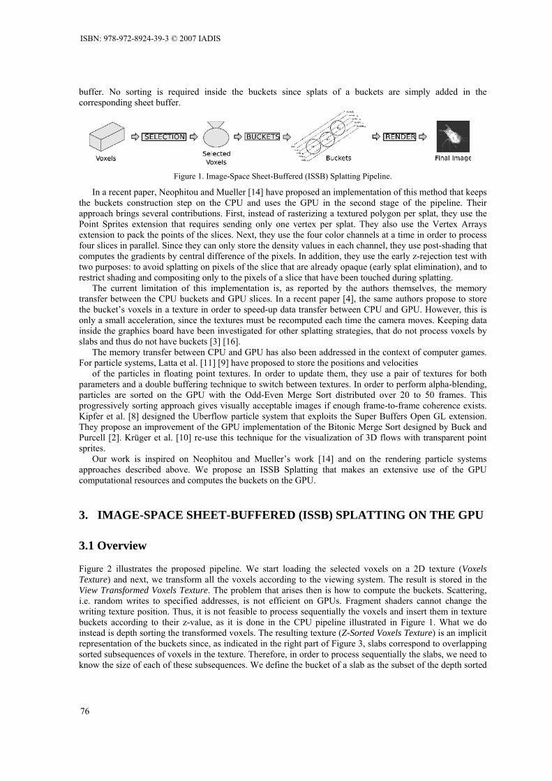
buffer. No sorting is required inside the buckets since splats of a buckets are simply added in the corresponding sheet buffer.

Figure 1. Image-Space Sheet-Buffered (ISSB) Splatting Pipeline.

In a recent paper, Neophitou and Mueller [14] have proposed an implementation of this method that keeps the buckets construction step on the CPU and uses the GPU in the second stage of the pipeline. Their approach brings several contributions. First, instead of rasterizing a textured polygon per splat, they use the Point Sprites extension that requires sending only one vertex per splat. They also use the Vertex Arrays extension to pack the points of the slices. Next, they use the four color channels at a time in order to process four slices in parallel. Since they can only store the density values in each channel, they use post-shading that computes the gradients by central difference of the pixels. In addition, they use the early z-rejection test with two purposes: to avoid splatting on pixels of the slice that are already opaque (early splat elimination), and to restrict shading and compositing only to the pixels of a slice that have been touched during splatting.

The current limitation of this implementation is, as reported by the authors themselves, the memory transfer between the CPU buckets and GPU slices. In a recent paper [4], the same authors propose to store the bucket’s voxels in a texture in order to speed-up data transfer between CPU and GPU. However, this is only a small acceleration, since the textures must be recomputed each time the camera moves. Keeping data inside the graphics board have been investigated for other splatting strategies, that do not process voxels by slabs and thus do not have buckets [3] [16].

The memory transfer between CPU and GPU has also been addressed in the context of computer games. For particle systems, Latta et al. [11] [9] have proposed to store the positions and velocities

of the particles in floating point textures. In order to update them, they use a pair of textures for both parameters and a double buffering technique to switch between textures. In order to perform alpha-blending, particles are sorted on the GPU with the Odd-Even Merge Sort distributed over 20 to 50 frames. This progressively sorting approach gives visually acceptable images if enough frame-to-frame coherence exists. Kipfer et al. [8] designed the Uberflow particle system that exploits the Super Buffers Open GL extension. They propose an improvement of the GPU implementation of the Bitonic Merge Sort designed by Buck and Purcell [2]. Krüger et al. [10] re-use this technique for the visualization of 3D flows with transparent point sprites.

Our work is inspired on Neophitou and Mueller’s work [14] and on the rendering particle systems approaches described above. We propose an ISSB Splatting that makes an extensive use of the GPU computational resources and computes the buckets on the GPU.

3. IMAGE-SPACE SHEET-BUFFERED (ISSB) SPLATTING ON THE GPU

3.1 Overview

Figure 2 illustrates the proposed pipeline. We start loading the selected voxels on a 2D texture (Voxels Texture) and next, we transform all the voxels according to the viewing system. The result is stored in the View Transformed Voxels Texture. The problem that arises then is how to compute the buckets. Scattering, i.e. random writes to specified addresses, is not efficient on GPUs. Fragment shaders cannot change the writing texture position. Thus, it is not feasible to process sequentially the voxels and insert them in texture buckets according to their z-value, as it is done in the CPU pipeline illustrated in Figure 1. What we do instead is depth sorting the transformed voxels. The resulting texture (Z-Sorted Voxels Texture) is an implicit representation of the buckets since, as indicated in the right part of Figure 3, slabs correspond to overlapping sorted subsequences of voxels in the texture. Therefore, in order to process sequentially the slabs, we need to know the size of each of these subsequences. We define the bucket of a slab as the subset of the depth sorted

ISBN: 978-972-8924-39-3 © 2007 IADIS

76

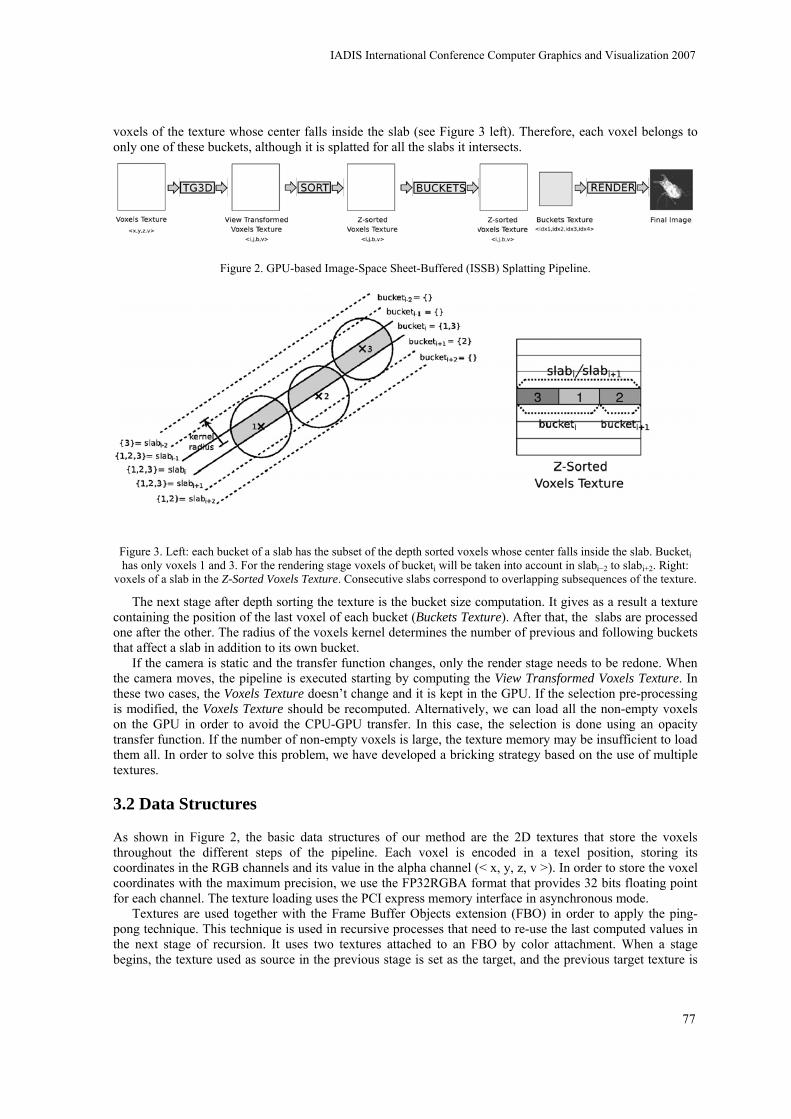
voxels of the texture whose center falls inside the slab (see Figure 3 left). Therefore, each voxel belongs to only one of these buckets, although it is splatted for all the slabs it intersects.

Figure 2. GPU-based Image-Space Sheet-Buffered (ISSB) Splatting Pipeline.

Figure 3. Left: each bucket of a slab has the subset of the depth sorted voxels whose center falls inside the slab. Bucketi has only voxels 1 and 3. For the rendering stage voxels of bucketi will be taken into account in slabi−2 to slabi+2. Right:

voxels of a slab in the Z-Sorted Voxels Texture. Consecutive slabs correspond to overlapping subsequences of the texture.

The next stage after depth sorting the texture is the bucket size computation. It gives as a result a texture containing the position of the last voxel of each bucket (Buckets Texture). After that, the slabs are processed one after the other. The radius of the voxels kernel determines the number of previous and following buckets that affect a slab in addition to its own bucket.

If the camera is static and the transfer function changes, only the render stage needs to be redone. When the camera moves, the pipeline is executed starting by computing the View Transformed Voxels Texture. In these two cases, the Voxels Texture doesn’t change and it is kept in the GPU. If the selection pre-processing is modified, the Voxels Texture should be recomputed. Alternatively, we can load all the non-empty voxels on the GPU in order to avoid the CPU-GPU transfer. In this case, the selection is done using an opacity transfer function. If the number of non-empty voxels is large, the texture memory may be insufficient to load them all. In order to solve this problem, we have developed a bricking strategy based on the use of multiple textures.

3.2 Data Structures

As shown in Figure 2, the basic data structures of our method are the 2D textures that store the voxels throughout the different steps of the pipeline. Each voxel is encoded in a texel position, storing its coordinates in the RGB channels and its value in the alpha channel (< x, y, z, v >). In order to store the voxel coordinates with the maximum precision, we use the FP32RGBA format that provides 32 bits floating point for each channel. The texture loading uses the PCI express memory interface in asynchronous mode.

Textures are used together with the Frame Buffer Objects extension (FBO) in order to apply the ping-pong technique. This technique is used in recursive processes that need to re-use the last computed values in the next stage of recursion. It uses two textures attached to an FBO by color attachment. When a stage begins, the texture used as source in the previous stage is set as the target, and the previous target texture is

IADIS International Conference Computer Graphics and Visualization 2007

77

the current source texture. Specifically, we use the pingpong technique in the sorting stage to compute the Z-Sorted Voxels Texture.

In addition to FBO, we use Vertex Buffer Objects (VBO) with the Render to Vertex Buffer (R2VB) technique that lets us create VBO using the values of a 2D texture. We use the Pixel Buffer Object (PBO) extension to load the 2D texture values onto the VBO. This keeps all the data flow inside the GPU. We use R2VB in the Buckets Texture construction and for the rendering stage.

3.3 Viewing Transform (VT)

This stage computes the View Transformed Voxels Texture from the Voxels Texture. We use a fragment shader that transforms the coordinates of the voxels stored as RGB values in the source texels according to the viewing matrix. For each texel, the fragment shader stores the 2D raster coordinates of the voxel’s projection in the R and G channel of the target texture, its depth value in the G channel and the voxel property value in the alpha channel (< i, j, b, v >).

3.4 GPGPU sorting (SORT)

The challenge of designing GPGPU sorting algorithms is to exploit as best as possible the parallel nature of the GPU architecture. Data-driven sorting algorithms such as Quicksort, that are the fastest on CPU, are not suitable for GPU implementation. This is why existing GPU sorting methods, basically Odd-Even Merge Sort and Bitonic Sort, are network sorting data-independent strategies. Current GPU implementations of Bitonic Sort [6] are much faster than Odd-Even Merge. We have used Govindaraju et al.’s [5] GPU implementation of the bitonic sort. It sorts an array of < key, value > pairs. It uses the Multiple Render Target (MRT) extension to efficiently store the keys and the values. One render target stores the keys and the other the values, and a one-to-one correspondence exists between the two textures. This allows us keeping four instances in one RGBA texel.

The method takes as input a CPU array. In our case, the view transformed voxels to sort are already in the GPU. The sorting key is the depth voxel value b. We use a fragment shader on the View Transformed Voxels Texture that fills the render targets with the b texel values as the key and a voxel index in the texture as the value. Once sorting is finished, another fragment shader fills the Z-Sorted Voxels Texture from the sorted render targets.

3.5 Bucket Size Computation (BUCKETS)

In this stage of the pipeline, we compute on the GPU the Buckets Texture that stores the position of the last voxel of each bucket (bucket boundary voxel). This texture cannot be computed directly from the Z-Sorted Voxels Texture using fragment shaders because there is no relationship between these two textures. The Z-Sorted Voxels Texture contains all the selected voxels, whereas the Buckets Texture contains only one voxel per bucket. Therefore, we need a vertex shader capable of writing at specified positions on a texture. However, determining if a voxel is bucket boundary requires to compute its bucket and compare it to the bucket of the following voxel in the Z-Sorted Voxels Texture. This would be very expensive in a vertex shader, because it requires a texture fetch for each voxel, and current vertex shaders do no implement efficiently this operation. For this, we have splitted the computation of the Buckets Texture into two steps: first, we compute the bucket boundary voxels using a fragment shader and next, we construct the Bucket Texture using a vertex shader.

In the first step, we render the Z-Sorted Voxels Texture into an auxiliary texture that indicates for each voxel if it is bucket boundary or not. This auxiliary texture stores for each voxel the coordinates of its corresponding bucket in the Bucket Texture in the R and G channels. In the B channel, it stores a false z value inside the viewing frustum if the voxel is bucket boundary and outside otherwise. The alpha channel stores the index of the voxel in the Z-Sorted Voxels Texture (see Figure 4).

The second step uses this auxiliary texture as a VBO and renders it using glPoints of size one. The points corresponding to non bucket boundary voxels are rejected in the early-depth test. Thus, only the bucket boundary voxels are rendered in the Bucket Texture. The shader writes in the texture only the index of the voxel in the Z-Sorted Voxels Texture.

ISBN: 978-972-8924-39-3 © 2007 IADIS

78

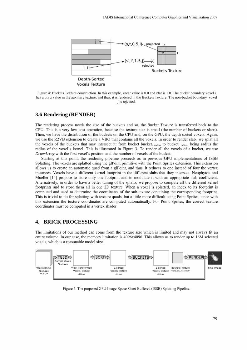
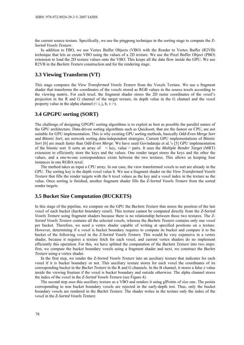
Figure 4:.Buckets Texture construction. In this example, znear value is 0.0 and zfar is 1.0. The bucket boundary voxel i

has a 0.5 z value in the auxiliary texture, and thus, it is rendered in the Buckets Texture. The non-bucket boundary voxel j is rejected.

3.6 Rendering (RENDER)

The rendering process needs the size of the buckets and so, the Bucket Texture is transferred back to the CPU. This is a very low cost operation, because the texture size is small (the number of buckets or slabs). Then, we have the distribution of the buckets on the CPU and, on the GPU, the depth sorted voxels. Again, we use the R2VB extension to create a VBO that contains all the voxels. In order to render slabi, we splat all the voxels of the buckets that may intersect it: from bucket bucketi−radius to bucketi+radius, being radius the radius of the voxel’s kernel. This is illustrated in Figure 3. To render all the voxels of a bucket, we use DrawArray with the first voxel’s position and the number of voxels of the bucket.

Starting at this point, the rendering pipeline proceeds as in previous GPU implementations of ISSB Splatting. The voxels are splatted using the glPoint primitive with the Point Sprites extension. This extension allows us to create an automatic quad from a glPoint, and thus, it reduces to one instead of four the vertex instances. Voxels have a different kernel footprint in the different slabs that they intersect. Neophytou and Mueller [14] propose to store only one footprint and to modulate it with an appropriate slab coefficient. Alternatively, in order to have a better tuning of the splatts, we propose to compute all the different kernel footprints and to store them all in one 2D texture. When a voxel is splatted, an index to its footprint is computed and used to determine the coordinates of the sub-texture containing the corresponding footprint. This is trivial to do for splatting with texture quads, but a little more difficult using Point Sprites, since with this extension the texture coordinates are computed automatically. For Point Sprites, the correct texture coordinates must be computed in a vertex shader.

4. BRICK PROCESSING

The limitations of our method can come from the texture size which is limited and may not always fit an entire volume. In our case, the memory limitation is 4096x4096. This allows us to render up to 16M selected voxels, which is a reasonable model size.

Figure 5. The proposed GPU Image-Space Sheet-Buffered (ISSB) Splatting Pipeline.

IADIS International Conference Computer Graphics and Visualization 2007

79

However, when larger models need to be processed, we subdivide them using bricks [15]. Each brick is stored on the GPU as a 2D texture (Voxel Bricks Texture). The maximum number of bricks is given by the texture memory size. The new pipeline is represented in Figure 5. Bricks are computed by subdividing the volume into octants. They are traversed orderly according to the camera position.

A drawback of bricking is that overlapping kernels at the boundary between bricks can be composed in incorrect order. However, bricking is needed when the number of selected voxels is large, and thus the ratio pixels per voxel is generally low. In this case, kernels do not overlap very much and artifacts at the brick boundary are not perceivable.

For very large datasets such that all the bricks cannot be loaded in GPU-memory, before processing a brick, we check if it is already in the GPU. Otherwise, we need to transfer it from the CPU.

5. RESULTS

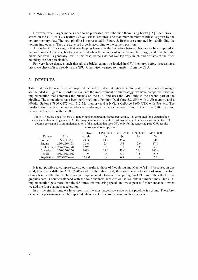
Table 1 shows the results of the proposed method for different datasets. Color plates of the rendered images are included in Figure 6. In order to evaluate the improvement of our strategy, we have compared it with an implementation that computes the buckets on the CPU and uses the GPU only in the second part of the pipeline. The simulations have been performed on a Pentium Dual Core 3.2 GHz with 3 Gb memory and a NVidia GeForce 7900 GTX with 512 Mb memory and a NVidia GeForce 8800 GTX with 768 Mb. The results show that our method accelerates rendering in a factor between 2 and 2.5 with the 7900 card and between 6.5 and 9.5 with the 8800.

Table 1. Results. The efficiency of rendering is measured in frames per second. It is computed for a visualization sequence with a moving camera. All the images are rendered with semi-transparency. Frames per second in the CPU

column correspond to an implementation of the method that uses GPU only for the rendering part. GPU results correspond to our pipeline.

It is not possible to compare exactly our results to those of Neophitou and Mueller’s [14], because, on one hand, they use a different GPU (6800) and, on the other hand, they use the acceleration of using the four channels in parallel that we have not yet implemented. However, comparing our CPU times, the effect of the graphics card is counterbalanced with the four channels acceleration, so we obtain similar times. Our GPU implementation gets more than the 6.5 times this rendering speed, and we expect to further enhance it when we add the four channels acceleration.

In all the simulations, we have seen that the most expensive stage of the pipeline is sorting. Therefore, even better performance can be expected when new GPU-based sorting methods appear.

Dataset

Size

Effective voxels

CPU-7900 fps

GPU-7900 fps

CPU-8800 fps

GPU-8800 fps

Lobster 324x301x56 233K 13.2 35.4 15 140 Engine 256x256x128 1.3M 2.4 5.6 2.6 17.8 BostonTeapo 256x256x178 4.9M 0.8 1.8 0.8 6.6 Aneurism 256x256x256 169K 18.4 43.4 21.4 160.4 Bonsai 256x256x256 1.3M 2.4 5.6 2.8 25.2 StagBettle 832x832x494 13.8M 0.4 0.8 0.4 2.6

ISBN: 978-972-8924-39-3 © 2007 IADIS

80

Figure 5. The proposed GPU Image-Space Sheet-Buffered (ISSB) Splatting Pipeline.

6. CONCLUSIONS

Splatting provides high quality images and it can be used for voxel models as well as for point- based surface models, that are unsuitable for ray-casting based rendering.

In this paper, we have proposed a new Image-space Sheet-Buffered (ISSB) Splatting design that creates and manages the buckets on the GPU. Our implementation achieves frame rates between 6.5 and 9.5 faster than methods that use the GPU only for the rendering part. Moreover, the evolution of the speed of GPU algorithms is dramatical in relation to the evolution of CPU algorithms. Therefore, as GPUs will evolve, the cost of the most expensive part of our pipeline, sorting, will reduce, and thus, much higher rendering speed-ups are expected.

Our future research is to try to adapt this method to multi-modal data that require performing a fusion of the property values of the different modalities either in the splatting stage or during the buckets construction depending on if post-shading or pre-shading is applied. Furthermore, we will investigate how to render time-varying data using this strategy taking into account frame-to-frame coherence.

ACKNOWLEDGEMENT

This work has been partially funded by the project MAT2005-07244-C03-03 and the Institut de Bioenginyeria de Catalunya (IBEC).

IADIS International Conference Computer Graphics and Visualization 2007

81

REFERENCES

[1] M. Botsch, A. Hornung, M. Zwicker, and L. Kobbelt. High quality surface splatting on todays GPU. In M. Pauly and M. Zwicker, editors, EG Symp.on Point-based graphics, pages 1–8, 2005.

[2] I. Buck and T. Purcell. A Toolkit for Computation on GPUs, chapter GPU Gems: Programming Techniques, Tips, and Tricks for Real-Time Graphics, R. Fernando Editor. Addison-Wesley, 2004.

[3] W. Chen, L. Ren, M. Zwicker, and H. Pfister. Hardware-accelerated adaptive EWA volume splatting. In IEEE Visualization’04, pages 67–74, 2004.

[4] N. Neophytou et al. Gpu-accelerated volume splatting with elliptical rbfs. pages 13–20, 2006. [5] N. K. Govindaraju, N. Raghuvanshi, M. Henson, and D. Manocha. A cache-efficient sorting algorithm for database

and data mining computations using graphics processors. Technical report, UNC Tech. Report, 2005. [6] A. Greß and G. Zachmann. GPU-ABiSort: Optimal parallel sorting on stream architectures. In IEEE International

Parallel and Distributed Processing Symposium, 2006. [7] J. Huang, K. Mueller, N. Shareef, and R. Crawfis. Fastsplats: optimized splatting on rectilinear grids. In IEEE

Visualization’00, pages 219–226. IEEE Computer Society Press, 2000. [8] P. Kipfer, M. Segal, and R. Westermann. Uberflow: a gpu-based particle engine. In ACM SIGGRAPH/EG

Conference on Graphics hardware, pages 115–122. ACM Press, 2004. [9] A. Kolb, L. Latta, and C. Rezk-Salama. Hardware-based simulation and collision detection for large particle

systems. In HWWS ’04: Proceedings of the ACM SIGGRAPH/EUROGRAPHICS conference on Graphics hardware, pages 123–131. ACM Press, 2004.

[10] J. Kruger, P. Kipfer, P. Kondratieva, and R. Westermann. A particle system for interactive visualization of 3D flows. IEEE Transactions on Visualization and Computer Graphics, 11(6):744– 756, 2005.

[11] L. Latta. Game developers Conference, chapter Building a million particle system. Gamasutra, 2004. [12] H. Mueller and R. Crawfis. Eliminating popping artifacts in sheet buffer-based splatting. IEEE Visualization’98,

pages 239–246, 1998. [13] K. Mueller, N. Shareef, J. Huang, and R. Crawfis. High-quality splatting on rectilinear grids with efficient culling of

occluded voxels. IEEE Trans. on Visual. and Computer Graphics, 5(2):116–134, 1999. [14] N. Neophytou and K. Mueller. GPU accelerated image aligned splatting. In I. Fujishiro and E. Gröller, editors,

Volume Graphics, pages 197–205, 2005. [15] D. Ruijters and A. Vilanova. Optimizing gpu volume rendering. WSCG - Winter School of Computer Graphics,

14:9–16, 2006. [16] F. Vega, P. Hastreiter, R. Fahlbusch, and G. Greiner. High performance volume splatting for visualization of

neurovascular data. In IEEE Visualization’05, pages 271–278, 2005. [17] L.Westover. Interactive volume rendering. In Volume Visualization Workshop, pages 9–16, 1989. [18] D. Xu and R. Crawfis. Efficient splatting using modern graphics hardware. Journal of graphics tools, 8(4):1–21,

2004. [19] M. Zwicker, J. Rasanen, M. Botsch, C. Dachsbacher, and M. Pauly. Perspective accurate splatting. In Graphics

interface’04, pages 247–254, 2004.

ISBN: 978-972-8924-39-3 © 2007 IADIS

82