Image segmentation based on merging of sub-optimalsegmentations

Juan C. Pichel1, David E. Singh and Francisco F. RiveraDept. Electronica e Computacion

Universidade de Santiago de Compostela, Galicia, Spain

E-Mail : {jcpichel, david, fran}@dec.usc.es

Abstract

In this paper a heuristic segmentation algorithm is presented based on the oversegmentation of an image.

The method uses a set of different segmentations of the image produced previously by standard techniques.

These segmentations are combined to create the oversegmented image. They can be performed using differ-

ent techniques or even the same technique with different initial conditions. Based on this oversegmentation a

new method of region merging is proposed. The merging process is guided using only information about the

behavior of each pixel in the input segmentations. Therefore, the results are an adequate combination of the

features of these segmentations, allowing to mask the negative particularities of individual segmentations.

In this work the quality of the proposal is analyzed with both artificial and real images using a evaluation

function as case of study. The results show that our algorithm produces high quality global segmentations

from a set of low quality segmentations with reduced execution times.

Keywords: Segmentation, Region-merging heuristic, Segmentation evaluation.

1 Introduction

The problem of the segmentation of images generally implies the partitioning of an image into a number of

homogeneous regions, so that joining two of these neighboring regions gives rise to another heterogeneous

region. Many ways of defining the homogeneity of a region exist, depending on the context of the appli-

cation. Moreover, a wide variety of methods and algorithms are available to deal with the problem of the

segmentation of images (Fu and Mui, 1981; Haralick and Shapiro, 1985; Pal and Pal, 1993). These methods

can be broadly classified in four categories (Zhu and Yuille, 1996):

• Edge-based techniques.

• Region-based techniques.1Corresponding author. Tel.: +34 981563100 ext. 13564; fax: +34 981528012; E-Mail: jcpichel@dec.usc.es

1

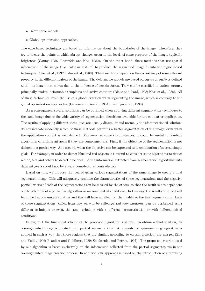
• Deformable models.

• Global optimization approaches.

The edge-based techniques are based on information about the boundaries of the image. Therefore, they

try to locate the points in which abrupt changes occur in the levels of some property of the image, typically

brightness (Canny, 1986; Rosenfeld and Kak, 1982). On the other hand, those methods that use spatial

information of the image (e.g. color or texture) to produce the segmented image fit into the region-based

techniques (Chen et al., 1992; Sahoo et al., 1988). These methods depend on the consistency of some relevant

property in the different regions of the image. The deformable models are based on curves or surfaces defined

within an image that moves due to the influence of certain forces. They can be classified in various groups,

principally snakes, deformable templates and active contours (Blake and Isard, 1998; Kass et al., 1988). All

of these techniques avoid the use of a global criterion when segmenting the image, which is contrary to the

global optimization approaches (Geman and Geman, 1984; Kanungo et al., 1998).

As a consequence, several solutions can be obtained when applying different segmentation techniques to

the same image due to the wide variety of segmentation algorithms available for any context or application.

The results of applying different techniques are usually dissimilar and normally the aforementioned solutions

do not indicate evidently which of these methods performs a better segmentation of the image, even when

the application context is well defined. Moreover, in some circumstances, it could be useful to combine

algorithms with different goals if they are complementary. First, if the objective of the segmentation is not

defined in a precise way. And second, when the objective can be expressed as a combination of several simple

goals. For example, in order to detect blue and red objects it is useful to consider some algorithms to detect

red objects and others to detect blue ones. So the information extracted from segmentation algorithms with

different goals should not be always considered as contradictory.

Based on this, we propose the idea of using various segmentations of the same image to create a final

segmented image. This will adequately combine the characteristics of these segmentations and the negative

particularities of each of the segmentations can be masked by the others, so that the result is not dependent

on the selection of a particular algorithm or on some initial conditions. In this way, the results obtained will

be unified in one unique solution and this will have an effect on the quality of the final segmentation. Each

of these segmentations, which from now on will be called partial segmentations, can be performed using

different techniques or even, the same technique with a different parametrization or with different initial

conditions.

In Figure 1 the functional scheme of the proposed algorithm is shown. To obtain a final solution, an

oversegmented image is created from partial segmentations. Afterwards, a region-merging algorithm is

applied in such a way that those regions that are similar, according to certain criterion, are merged (Zhu

and Yuille, 1996; Beaulieu and Goldberg, 1989; Shafarenko and Petrou, 1997). The proposed criterion used

by our algorithm is based exclusively on the information collected from the partial segmentations in the

oversegmented image creation process. In addition, our approach is based on the introduction of a repulsing

2

Image

Segmentation Segmentation Segmentation

1 2 N

Partial Segmentations

Combining

Oversegmented Image

Merging

Segmented Image

Info

rmat

ion

Figure 1: Functional scheme of the proposed algorithm.

force between neighboring regions that measures the tendency of these to remain separated. The structure

of this work is as follows. In Section 2 the concept of shadowed zones is introduced and how we can obtain

the oversegmented image from the partial segmentations is explained. In Section 3 the concept of the force

of repulsion between regions that indicates the tendency of two regions to merge or remain separated in the

final segmentation is introduced. Section 4 describes the merging process, while Section 5 shows the results

using, as case of study, a segmentation evaluation function as stopping criterion of the merging process.

Finally, Section 6 presents the main conclusions of this work.

2 Generation of the oversegmented image

The segmentation of an image can be considered as a labeling problem, in the sense that those pixels that

belong to the same region have been assigned the same label, which can be specified in terms of a set of

states or a set of labels. Let H be a discrete set with m states, H = {1, 2, ..., m} and let L be the set of

labels. In our case, a state represents a region of the Euclidian space of the image (set of pixels). Labeling

is not more than a function that assigns one of the labels of L to each of the states of H.

Generally, the objective of the segmentation algorithms based on regions is the labeling of all the pixels

of the image. In many cases, in the final stages of the process, this situation causes pixels to be included in

regions from which they have very low similarity levels, thereby creating regions with low homogeneity. To

3

(a)

(b)

(c)

Figure 2: Examples of partial segmentations of image Test3 applying the SRG algorithm (a) without

shadowed zones and (b) using shadowed zones. The oversegmented image produced by the combination of

the partial segmentations of (b) is shown in (c).

avoid this effect we propose the inclusion of a specific threshold as a possible solution. This threshold would

be such that those pixels with a low degree of similarity with respect to the target region are not included in

it, remaining unlabeled. The set of unlabeled pixels will be called shadowed zones. Therefore, a pixel, after

the partial segmentation, can be labeled and thus belongs to a region, or it can be included in a shadowed

zone.

As an example, we checked the effect of using shadowed zones in a test image, performing the partial

segmentations using the Seeded Region Growing algorithm (SRG) introduced by Mehnert and Jackway

(1997). The process begins with a set of pixels, called seeds, which will be the basis for the determination

of the regions. It continues including, incrementally, the pixels on their boundaries according to some given

criterion to measure the similitude. Mehnert and Jackway use as criterion the difference between the grey

intensity of the pixel under consideration and the average of the intensities of the pixels that already form

part of the region. Figure 2(a) shows the boundaries of three different partial segmentations of the image

Test3 by using 20 seeds placed randomly. In this type of algorithm, the initial number of seeds determines

the number of regions of the segmented image. Moreover, the quality of the result of the algorithm depends

4

Region B

Region D

Region E

Region C

Region A

0

1

2

3

4

0

1 2 3

4

Shadowed Zone

Figure 3: Example of the generation of an oversegmented image from three partial segmentations of 5 × 5

pixels with three regions each one. The oversegmented image presents five regions.

in a great extend on the position of the seeds. As we have mentioned, the algorithm is forced to label all the

pixels of the image. This behavior becomes manifest in these images, in which some regions include pixels

with very low similitude. The quality of these segmentations is poor. By introducing a threshold in the level

of similitude, shadowed zones are created in the image. Three partial segmentations, using the same seeds

as Figure 2(a), with shadowed zones represented in grey, are shown in Figure 2(b). Note that, with the use

of shadowed zones, the number of correct regions detected by the segmentation increases significantly with

respect to the segmentation using the original algorithm. Despite of it, none of these segmentations achieve

the correct result.

Our proposal generates an oversegmented image as a combination of various partial segmentations in

which shadowed areas can exist. There are other segmentation techniques that create an oversegmented image

such as watershed algorithms (Haris et al., 1998). The oversegmentations obtained from these algorithms

can be used as input of our algorithm, but not as unique oversegmented image. That is because, as we

detail later, we need to collect, from different partial segmentations, the information that will guide the

merging process. In our algorithm an operation for intersecting all the partial segmentations is performed in

such a way that those pixels that belong to the same region in all the partial segmentations remain united

in one of the regions of the oversegmented image. Figure 3 shows a simple example of the creation of an

oversegmented image formed, in this case, from three partial segmentations. The first partial segmentation

presents a shadowed zone and two regions, whilst in each of the other two segmentations there are three

regions and no shadowed zones. In this example the oversegmented image consists of five regions.

If shadowed zones exist in some of the partial segmentations, they are considered as any other region in

the generation of the oversegmented image, although later, in the merging algorithm, they will be treated

differently. Another example is shown in Figure 2(c). It shows the oversegmented image created from the

partial segmentations of Figure 2(b).

5

3 Force of repulsion between regions

One important contribution of our proposal is that all the relevant information to obtain the final segmented

image is obtained exclusively from the different partial segmentations, both for creating the oversegmented

image and for applying the subsequent region-merging algorithm. It should be noted that this strategy does

not take into account local characteristics such as size, shade of average grey intensities, etc. Based on the

results obtained for all the pixels of the image in each of the partial segmentations, global conclusions are

obtained with respect to them. Without losing generality, in our algorithm we have chosen a second-order

neighborhood scheme, so that up to eight neighbors are defined for each pixel. In each partial segmentation

we can find any pair of neighboring pixels in one of the following four different states:

1. Both belong to same labeled region.

2. Both belong to different labeled regions.

3. Both belong to shadowed zones.

4. One belongs to a region and the other to a shadowed zone.

We define a function to efficiently collect this information that adds up each one of these possible states.

This function summarizes the state of any pair of neighboring pixels of the image. Thus, over N partial

segmentations, we can define the following counters for any pair of neighboring pixels i and j:

• n1(i, j) → Number of partial segmentations in which they have been in the same labeled region.

• n2(i, j) → Number of partial segmentations in which both have been in a shaded region.

• n3(i, j) → Number of partial segmentations in which they have been in different labeled regions.

• n4(i, j) → Number of partial segmentations in which only one of them has been in a shaded region.

It can be easily proven that the following properties are fulfilled:

nk(i, j) = nk(j, i), being k = 1, 2, 3 or 4 (1)

n1(i, j) + n2(i, j) + n3(i, j) + n4(i, j) = N (2)

In this way, those pixels i and j that belong to the same region in the oversegmented image should verify:

n3(i, j) = n4(i, j) = 0 (3)

Based on these counters, we define a force of repulsion between two neighboring pixels i and j that measures

the tendency of these pixels to be or not in the same region. We propose for this force a linear combination

of the above counters, given through the following equation:

fij = −C1 n1(i, j)− C2 n2(i, j) + C3 n3(i, j) + C4 n4(i, j) (4)

6

where Cn are parameters to weight each of the situations in which two neighboring pixels could be found.

Therefore, two different components can be identified in Equation 4: on one hand an attractive component

given by term −C1 n1(i, j) − C2 n2(i, j) that measures the tendency of these pixels to belong to the same

region, and on the other, a repulsive component given by term C3 n3(i, j) + C4 n4(i, j) that measures the

opposite. According with this equation we can see that the lesser the force fij , the greater is the tendency

for these pixels to belong to the same region. Additionally, we have that the pixels that belong to the same

region always verify that fij < 0.

For instance, let’s consider the force of repulsion fij among some pixels of the oversegmented image in

Figure 3. To simplify this example, the weight parameters of the Equation 4 are C1 = C2 = C3 = C4 = 1.

The counters for the neighboring pixels (0, 1) and (0, 2), are n1 = 3, n2 = n3 = n4 = 0, and therefore, we

obtain a force of repulsion fij = −3. For pixels (2, 1) and (2, 2), we have n1 = n2 = 0, n3 = 2, n4 = 1, that

causes an attraction force of fij = 3. Finally, for pixels (2, 3) and (2, 4) have n1 = 2, n3 = 1, n2 = n4 = 0,

and fij = −1.

Next we show an analysis to determine the way these parameters are related. C1 weights the tendency

of a pair of pixels to be in the same region. Initially, we consider the relationship between C1 and the

parameter that weights the situation in which two pixels belong to different regions (C3). At first sight it

seems adequate that both parameters must have the same value because the situations that they represent

seem symmetrically opposite. Nevertheless, as we have mentioned, one of the principal drawbacks of many

segmentation algorithms, specially the region based algorithms such as SRG, is that two seeds placed within

the same object in the image produce two different regions in the segmented image although it is only one

real region. For the merging algorithm to deal with this problem we must reward, in some way, that two

pixels belong to the same region in the oversegmented image. So we propose that C1 ≥ C3.

Respect to the parameter that weights the situation when two pixels belong to a shadowed zone (C2),

these pixels are not treated by the partial segmentation algorithm. Note that using shadowed zones the

dependence of the region based algorithm with the placing of the seeds decrease meaningfully. So, the fact

that two pixels belong to a shadowed zone in the partial segmentation, does not bring enough information

to decide if these pixels must belong to the same or to different regions, i.e., C2 must be small compared to

the other parameters.

Finally, the parameter that weights the situation in which one pixel belongs to a shadowed zone and

the other to a region (C4), provides important information because the partial segmentation decided not to

include it in a labeled region. Therefore, these pixels must belong to different regions to avoid the creation

of low homogeneity regions. So C4 ≥ C1.

According to all these topics, we summarize the relationships between the parameters as:

C4 ≥ C1 ≥ C3 ≥ C2 (5)

7

C

E

A

B D -1-1

3 1

-1

-1

0

3

3

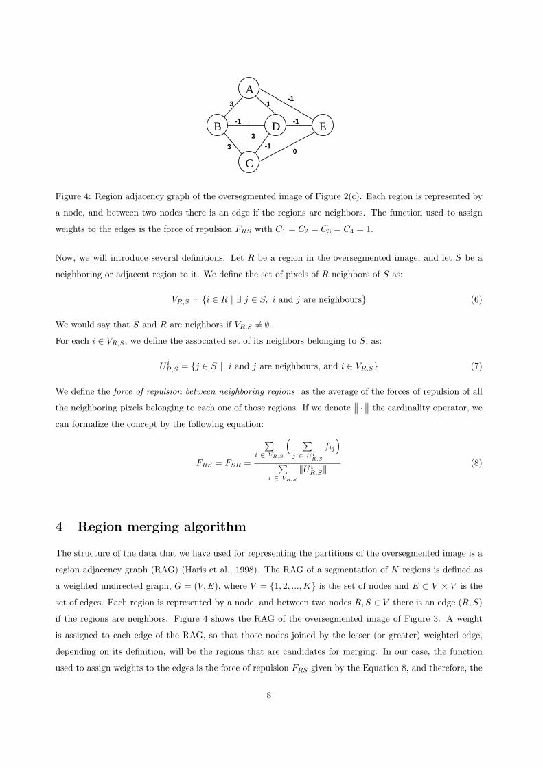
Figure 4: Region adjacency graph of the oversegmented image of Figure 2(c). Each region is represented by

a node, and between two nodes there is an edge if the regions are neighbors. The function used to assign

weights to the edges is the force of repulsion FRS with C1 = C2 = C3 = C4 = 1.

Now, we will introduce several definitions. Let R be a region in the oversegmented image, and let S be a

neighboring or adjacent region to it. We define the set of pixels of R neighbors of S as:

VR,S = {i ∈ R | ∃ j ∈ S, i and j are neighbours} (6)

We would say that S and R are neighbors if VR,S 6= ∅.For each i ∈ VR,S , we define the associated set of its neighbors belonging to S, as:

U iR,S = {j ∈ S | i and j are neighbours, and i ∈ VR,S} (7)

We define the force of repulsion between neighboring regions as the average of the forces of repulsion of all

the neighboring pixels belonging to each one of those regions. If we denote∥∥ ·

∥∥ the cardinality operator, we

can formalize the concept by the following equation:

FRS = FSR =

∑i ∈ VR,S

( ∑j ∈ Ui

R,S

fij

)

∑i ∈ VR,S

‖U iR,S‖

(8)

4 Region merging algorithm

The structure of the data that we have used for representing the partitions of the oversegmented image is a

region adjacency graph (RAG) (Haris et al., 1998). The RAG of a segmentation of K regions is defined as

a weighted undirected graph, G = (V, E), where V = {1, 2, ..., K} is the set of nodes and E ⊂ V × V is the

set of edges. Each region is represented by a node, and between two nodes R, S ∈ V there is an edge (R, S)

if the regions are neighbors. Figure 4 shows the RAG of the oversegmented image of Figure 3. A weight

is assigned to each edge of the RAG, so that those nodes joined by the lesser (or greater) weighted edge,

depending on its definition, will be the regions that are candidates for merging. In our case, the function

used to assign weights to the edges is the force of repulsion FRS given by the Equation 8, and therefore, the

8

DO i = 0, n-1

Find the minimum cost edge in (K-i)-RAG using the heap

Merge the selected pair of regions to get the (K-i-1)-RAG

Update the heap

END DO

Figure 5: Pseudo-code of the merging algorithm.

regions that are candidates for merging are those joined by the edge with least weight. In the example of

Figure 4, C1 = C2 = C3 = C4 = 1.

Using the RAG as input, we propose an iterative heuristic to deal with the problem of merging, so that

one merging is performed in each of the iterations, based on the weight of the edges. A data structure

adequate for storing the weights is a queue, which can be implemented using a heap (Knuth, 1973). All

the edges of the RAG are stored in the heap according to the weights, so that the first edge always has

the smallest weight. Evaluating the heap requires O(‖E‖). In each iteration of the merging algorithm, the

pair of regions that have the smallest weight are merged. One of the most useful properties of this iterative

algorithm, as we show later, is that the weight of the edge that occupies the first position of the heap always

grows.

Given the RAG of an initial partition of K regions denoted as (K − RAG), and a heap of its edges,

the RAG of the partition K − n is obtained using the merging algorithm described in the pseudo-code

of Figure 5. The K − RAG corresponds to the initial partition of the image, which in our case, is the

oversegmented image. Subsequently, an iterative process is applied, in which, in the i-th iteration, the two

regions with the smallest weight are merged. Once they have been merged, the list of edges is updated, and

the (K − i− 1)−RAG is obtained.

From the algorithm, it is inferred that n iterations are needed to obtain the (K − n)−RAG. Therefore,

one of the problems posed by this strategy is to establish the best value of n, i.e., the best number of

regions of the final segmented image. Different alternatives can be used. For example, using the property

of the growing value of the first term of the heap, a certain threshold can be selected to stop the iterations

when the value of the edge at the top of the heap exceeds it. The main drawback of this approach is

that it is not evident to determine a good threshold a priori. Another approach is the use of a method that

allows a numerical evaluation of the segmentation, and chooses the best threshold according to some selected

validation criterion.

5 A case of study: evaluation function Q

Most of the results obtained by segmenting an image are evaluated visually and qualitatively. The principal

problem is searching for an uniform criterion to evaluate the results. Different methods for evaluating the

9

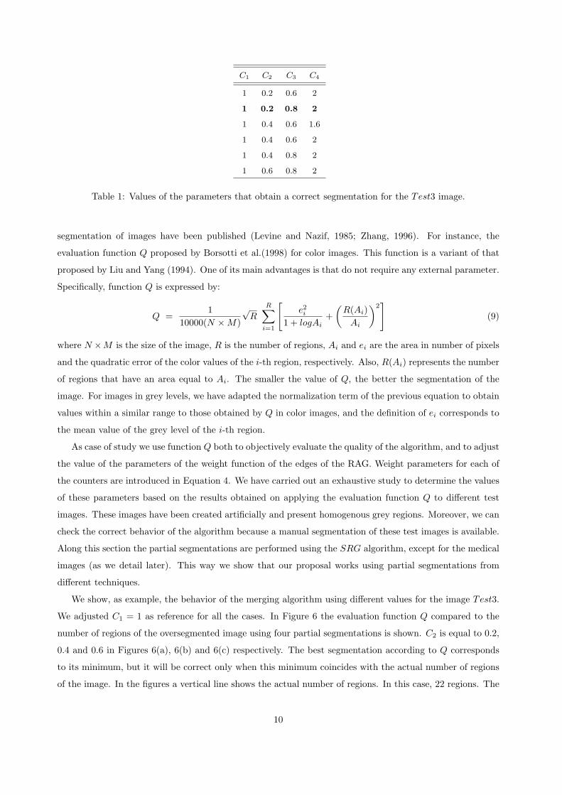
C1 C2 C3 C4

1 0.2 0.6 2

1 0.2 0.8 2

1 0.4 0.6 1.6

1 0.4 0.6 2

1 0.4 0.8 2

1 0.6 0.8 2

Table 1: Values of the parameters that obtain a correct segmentation for the Test3 image.

segmentation of images have been published (Levine and Nazif, 1985; Zhang, 1996). For instance, the

evaluation function Q proposed by Borsotti et al.(1998) for color images. This function is a variant of that

proposed by Liu and Yang (1994). One of its main advantages is that do not require any external parameter.

Specifically, function Q is expressed by:

Q =1

10000(N ×M)

√R

R∑

i=1

[e2i

1 + logAi+

(R(Ai)

Ai

)2]

(9)

where N ×M is the size of the image, R is the number of regions, Ai and ei are the area in number of pixels

and the quadratic error of the color values of the i-th region, respectively. Also, R(Ai) represents the number

of regions that have an area equal to Ai. The smaller the value of Q, the better the segmentation of the

image. For images in grey levels, we have adapted the normalization term of the previous equation to obtain

values within a similar range to those obtained by Q in color images, and the definition of ei corresponds to

the mean value of the grey level of the i-th region.

As case of study we use function Q both to objectively evaluate the quality of the algorithm, and to adjust

the value of the parameters of the weight function of the edges of the RAG. Weight parameters for each of

the counters are introduced in Equation 4. We have carried out an exhaustive study to determine the values

of these parameters based on the results obtained on applying the evaluation function Q to different test

images. These images have been created artificially and present homogenous grey regions. Moreover, we can

check the correct behavior of the algorithm because a manual segmentation of these test images is available.

Along this section the partial segmentations are performed using the SRG algorithm, except for the medical

images (as we detail later). This way we show that our proposal works using partial segmentations from

different techniques.

We show, as example, the behavior of the merging algorithm using different values for the image Test3.

We adjusted C1 = 1 as reference for all the cases. In Figure 6 the evaluation function Q compared to the

number of regions of the oversegmented image using four partial segmentations is shown. C2 is equal to 0.2,

0.4 and 0.6 in Figures 6(a), 6(b) and 6(c) respectively. The best segmentation according to Q corresponds

to its minimum, but it will be correct only when this minimum coincides with the actual number of regions

of the image. In the figures a vertical line shows the actual number of regions. In this case, 22 regions. The

10

0 5 10 15 20 25 30 35 40 45 500

200

400

600

800

1000

1200

1400

1600

Regions

Qc3 = 0.6 c4 = 1.2c3 = 0.6 c4 = 1.6c3 = 0.6 c4 = 2

0 5 10 15 20 25 30 35 40 45 500

200

400

600

800

1000

1200

1400

1600

Regions

Q

c3 = 0.8 c4 = 1.2c3 = 0.8 c4 = 1.6c3 = 0.8 c4 = 2

0 5 10 15 20 25 30 35 40 45 500

200

400

600

800

1000

1200

1400

1600

Regions

Q

c3 = 1 c4 = 1.2c3 = 1 c4 = 1.6c3 = 1 c4 = 2

0 5 10 15 20 25 30 35 40 45 500

200

400

600

800

1000

1200

1400

1600

Regions

Q

c3 = 0.6 c4 = 1.2c3 = 0.6 c4 = 1.6c3 = 0.6 c4 = 2

0 5 10 15 20 25 30 35 40 45 500

200

400

600

800

1000

1200

1400

1600

Regions

Q

c3 = 0.8 c4 = 1.2c3 = 0.8 c4 = 1.6c3 = 0.8 c4 = 2

0 5 10 15 20 25 30 35 40 45 500

200

400

600

800

1000

1200

1400

1600

Regions

Q

c3 = 1 c4 = 1.2c3 = 1 c4 = 1.6c3 = 1 c4 = 2

0 5 10 15 20 25 30 35 40 45 500

200

400

600

800

1000

1200

1400

1600

Regions

Q

c3 = 0.6 c4 = 1.2c3 = 0.6 c4 = 1.6c3 = 0.6 c4 = 2

0 5 10 15 20 25 30 35 40 45 500

200

400

600

800

1000

1200

1400

1600

Regions

Q

c3 = 0.8 c4 = 1.2c3 = 0.8 c4 = 1.6c3 = 0.8 c4 = 2

0 5 10 15 20 25 30 35 40 45 500

200

400

600

800

1000

1200

1400

1600

Regions

Q

c3 = 1 c4 = 1.2c3 = 1 c4 = 1.6c3 = 1 c4 = 2

Figure 6: Function Q compared to the number of regions of the oversegmented image using four partial

segmentations for Test3. In this case, C1 = 1 and (a) C2 = 0.2, (b) C2 = 0.4 and (c) C2 = 0.6.

other parameters, C3 and C4, will take different values as shown in Figure 6. In Table 1 the values of C1, C2,

C3 and C4 used by the merging algorithm to obtain a correct segmentation are shown. These values fulfil

the relationships of Equation 5. After applying this study to a broad set of test images we finally propose

the following values: C1 = 1, C2 = 0.2, C3 = 0.8 and C4 = 2. We have to mention that for all the images

we tested no correct segmentations are performed using parameters with values that do not fulfil Equation

5.

Next, as example, we show the results obtained for the images Test2 and Test3, that actually present

16 and 22 regions respectively. The segmentations obtained by applying the algorithm together with the

original image are shown in Figures 7 and 8. These figures also show the values of function Q compared to

the number of regions of the oversegmented images using 2, 3 and 4 different partial segmentations. From the

behavior of the Q function, we can infer that when the number of regions is equal to the number that each

image really has, Q presents its minimum. However, when only two partial segmentations are used, Q does

not converge adequately. This is because the created oversegmented image do not correctly detect the regions

11

(a) (b)

0 10 20 30 40 50 60 700

200

400

600

800

1000

1200

Regions

Q

2 partial segm.3 partial segm.4 partial segm.

16 regions

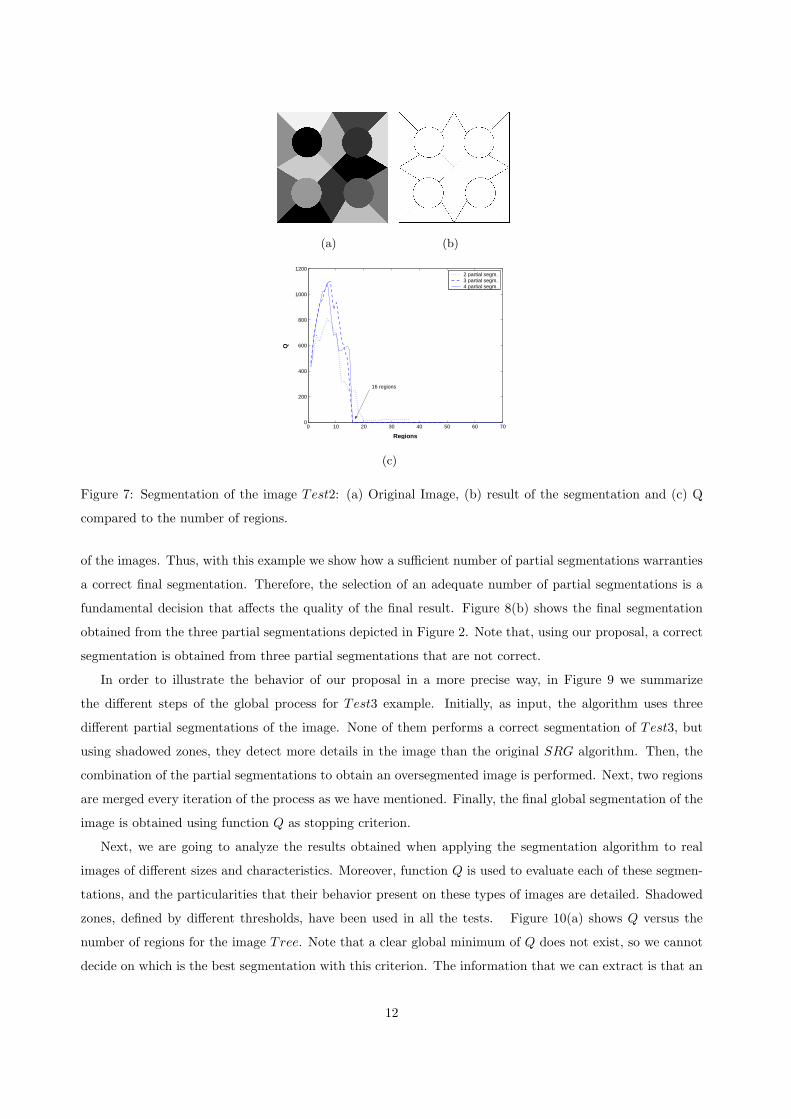
(c)

Figure 7: Segmentation of the image Test2: (a) Original Image, (b) result of the segmentation and (c) Q

compared to the number of regions.

of the images. Thus, with this example we show how a sufficient number of partial segmentations warranties

a correct final segmentation. Therefore, the selection of an adequate number of partial segmentations is a

fundamental decision that affects the quality of the final result. Figure 8(b) shows the final segmentation

obtained from the three partial segmentations depicted in Figure 2. Note that, using our proposal, a correct

segmentation is obtained from three partial segmentations that are not correct.

In order to illustrate the behavior of our proposal in a more precise way, in Figure 9 we summarize

the different steps of the global process for Test3 example. Initially, as input, the algorithm uses three

different partial segmentations of the image. None of them performs a correct segmentation of Test3, but

using shadowed zones, they detect more details in the image than the original SRG algorithm. Then, the

combination of the partial segmentations to obtain an oversegmented image is performed. Next, two regions

are merged every iteration of the process as we have mentioned. Finally, the final global segmentation of the

image is obtained using function Q as stopping criterion.

Next, we are going to analyze the results obtained when applying the segmentation algorithm to real

images of different sizes and characteristics. Moreover, function Q is used to evaluate each of these segmen-

tations, and the particularities that their behavior present on these types of images are detailed. Shadowed

zones, defined by different thresholds, have been used in all the tests. Figure 10(a) shows Q versus the

number of regions for the image Tree. Note that a clear global minimum of Q does not exist, so we cannot

decide on which is the best segmentation with this criterion. The information that we can extract is that an

12

(a) (b)

0 50 100 1500

200

400

600

800

1000

1200

1400

1600

1800

Regions

Q

2 partial segm.3 partial segm.4 partial segm.

22 regions

(c)

Figure 8: Segmentation of the image Test3: (a) Original Image, (b) result of the segmentation and (c) Q

compared to the number of regions.

interval of values of Q exists, shown in the figure with an arrow, in which the most adequate segmentations

can be found.

A detailed view of this zone when N = 8 is shown in Figure 10(b). In this case the local minimums can

be assessed, such as points a, b and c. The Tree original image and the segmentations that produce these

three points are shown in Figures 11(a), 11(b), 11(c) and 11(d) respectively. The first segmentation presents

just 12 regions, and although it produces a low Q, it has merged too many regions, with the consequent

loss of details in the image. The next segmentation presents 22 regions. Although the difference with other

possible segmentations is small, the Q value in this case is the minimum of the whole function. The same

conclusions can be obtained with the last segmentation, which has 44 regions, except that it has a higher Q

value than the previous case.

Therefore, based on these results we conclude that for the segmentation of real images, Q is very useful

for determining the set of the most adequate segmentations, but in most of the cases it is not going to be

sufficiently discriminating to select just one.

Table 2 summarizes the results obtained on a set of real images. N is the number of partial segmenta-

tions, Qmin is the minimum value of Q for this image, and R is the number of regions that presents this

segmentation. Moreover, S5% is the number of possible segmentations with a Q value that differs in a max-

imum of 5% with respect to Qmin, and Smin−5% and Smax−5% are the minimum and maximum number of

regions of a segmentation considered on S5% respectively.

13

Oversegmented Image

Iteration 10 Iteration 30 Iteration 45 Segmented Image

Partial Segmentations

Figure 9: Example of the behavior of the algorithm using Test3 as test image: Creation of the oversegmented

image and some iterations of the merging algorithm.

We can note that the number of adequate segmentations increases as reflected by the value of S5%. In

some cases, such as image Man, reaches more than 100. Function Q does not provide enough discriminating

information. It indicates the difficulty of determining the best segmentation. The number of regions that

could be detected varies for this image from 80 to 266 regions. However, for other images Q is quite

significant. In any case, the fact that the interval is wide, is not associated with the difficulty of determining

the best segmentation. Only the S5% segmentations of this interval differ by less than 5% with respect to

Qmin.

In order to illustrate the results of the algorithm, Figures 12 and 13 show some examples of segmentations

obtained for real images. Each of them corresponds to the value Qmin of the evaluation function. Note that

using our proposal high quality segmentations are obtained. In Figure 12 the partial segmentations were

obtained using the SRG algorithm. Figure 13 shows two medical images of the heart’s left ventricle obtained

using Single Photon Emission Computerized Tomography (spect). The partial segmentations of these

images were obtained using an active contour model algorithm described by Weickert and Kuhne (2003).

This algorithm was initialized using the method detailed in the Dosil et al. paper (2005). The medical

segmented images were validated visually by experts. In these examples, 8 different partial segmentations

to obtain each final segmented image were used.

Finally, Figure 14 shows the execution times compared to the number of iterations obtained on executing

14

0 50 100 150 200 250 300 350 4000

500

1000

1500

2000

2500

Regions

Q

3 partial segm.4 partial segm.8 partial segm.

(a)

10 20 30 40 50 60 70 80 90 1000

100

200

300

400

500

600

700

800

900

1000

Regions

Q

a

b

c

(b)

Figure 10: Segmentation of the image Tree: (a) Evaluation function Q and (b) detailed view for N=8.

(a) (b) (c) (d)

Figure 11: Segmentation of the image Tree: (a) Original Image, (b) 12 regions, (c) 22 regions and (d) 44

regions.

the merging algorithm on a Origin 200 system, for the images House and Peppers, with sizes of 256 × 256

and 512× 512 pixels respectively.

6 Conclusions

In this paper a new heuristic segmentation algorithm is presented, based on the use of various segmentations

of the same image that are combined to create an oversegmented image. These segmentations can be

performed using different techniques or even the same technique with different initial conditions. A region-

merging algorithm is then applied to this oversegmented image. The main idea of our proposal is to obtain

high quality segmentations from a set of low quality partial segmentations. A relevant aspect is that the

information obtained from the partial segmentations will, in fact, guide the merging process, in a such way

that the actual characteristics of each region or pixel are not taken into account.

We introduce the concept of force of repulsion between neighboring pixels that indicates quantitatively

their tendency to form part of different regions. The force of repulsion considers several situations in

which any two neighboring pixels can be found in all the partial segmentations that are used to create the

15

Images N Qmin R S5% Rmin−5% Rmax−5%

Tree 3 334.2 23 6 24 31

4 395.2 25 12 17 50

8 333.3 22 7 12 24

MIT 3 1446 50 18 21 58

4 1096.9 55 10 54 64

8 1092.5 64 8 65 72

House 3 125.8 35 8 30 38

4 144.5 24 6 25 30

8 126.9 42 17 30 49

Lena 4 289.2 73 17 52 107

6 285.2 76 21 68 90

8 280.1 68 14 61 83

Peppers 3 283.5 56 8 57 64

4 294.1 81 25 82 109

6 357.6 76 23 69 96

Man 3 604.5 166 105 101 265

4 629.2 168 103 80 266

6 561.1 120 49 97 146

Table 2: Summary of results for real images.

oversegmented image. In this context, we introduce the concept of shadowed zone. The shadowed zones are

groups of pixels that differ in their intensity level a certain threshold from the region in which they could be

included. Introducing this concept in the region-based algorithms, regions with low levels of homogeneity

are avoided improving the quality of the whole process. Note that, given that the shadowed zones are not

treated by the algorithm, the information that can be extracted from these zones is minimum.

To deal with the problem of region merging we propose an iterative heuristic to merge the regions with

the lowest force of repulsion in each iteration. We use a weighted graph and a heap for its management.

As stopping criterion of the merging algorithm we can use different alternatives. As case of study we apply

a function to evaluate the quality of the segmentation. This function has the advantage that it does not

require any type of external parameters. Moreover, it has been used to adjust the parameters that define

the force of repulsion between neighboring pixels.

Once the algorithm has been tested on a group of artificial test images, we apply the algorithm to a

significant group of real images that have different sizes and characteristics, demonstrating the benefits of

our proposal.

16

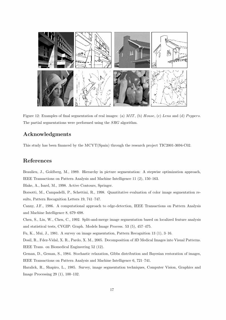
Figure 12: Examples of final segmentation of real images: (a) MIT , (b) House, (c) Lena and (d) Peppers.

The partial segmentations were performed using the SRG algorithm.

Acknowledgments

This study has been financed by the MCYT(Spain) through the research project TIC2001-3694-C02.

References

Beaulieu, J., Goldberg, M., 1989. Hierarchy in picture segmentation: A stepwise optimization approach,

IEEE Transactions on Pattern Analysis and Machine Intelligence 11 (2), 150–163.

Blake, A., Isard, M., 1998. Active Contours, Springer.

Borsotti, M., Campadelli, P., Schettini, R., 1998. Quantitative evaluation of color image segmentation re-

sults, Pattern Recognition Letters 19, 741–747.

Canny, J.F., 1986. A computational approach to edge-detection, IEEE Transactions on Pattern Analysis

and Machine Intelligence 8, 679–698.

Chen, S., Lin, W., Chen, C., 1992. Split-and-merge image segmentation based on localized feature analysis

and statistical tests, CVGIP: Graph. Models Image Process. 53 (5), 457–475.

Fu, K., Mui, J., 1981. A survey on image segmentation, Pattern Recognition 13 (1), 3–16.

Dosil, R., Fdez-Vidal, X. R., Pardo, X. M., 2005. Decomposition of 3D Medical Images into Visual Patterns.

IEEE Trans. on Biomedical Engineering 52 (12).

Geman, D., Geman, S., 1984. Stochastic relaxation, Gibbs distribution and Bayesian restoration of images,

IEEE Transactions on Pattern Analysis and Machine Intelligence 6, 721–741.

Haralick, R., Shapiro, L., 1985. Survey, image segmentation techniques, Computer Vision, Graphics and

Image Processing 29 (1), 100–132.

17

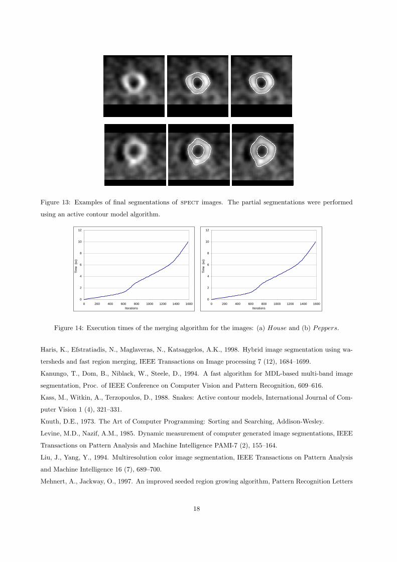
Figure 13: Examples of final segmentations of spect images. The partial segmentations were performed

using an active contour model algorithm.

0

2

4

6

8

10

12

0 200 400 600 800 1000 1200 1400 1600Iterations

Tim

e(s

c)

0

2

4

6

8

10

12

0 200 400 600 800 1000 1200 1400 1600Iterations

Tim

e(s

c)

Figure 14: Execution times of the merging algorithm for the images: (a) House and (b) Peppers.

Haris, K., Efstratiadis, N., Maglaveras, N., Katsaggelos, A.K., 1998. Hybrid image segmentation using wa-

tersheds and fast region merging, IEEE Transactions on Image processing 7 (12), 1684–1699.

Kanungo, T., Dom, B., Niblack, W., Steele, D., 1994. A fast algorithm for MDL-based multi-band image

segmentation, Proc. of IEEE Conference on Computer Vision and Pattern Recognition, 609–616.

Kass, M., Witkin, A., Terzopoulos, D., 1988. Snakes: Active contour models, International Journal of Com-

puter Vision 1 (4), 321–331.

Knuth, D.E., 1973. The Art of Computer Programming: Sorting and Searching, Addison-Wesley.

Levine, M.D., Nazif, A.M., 1985. Dynamic measurement of computer generated image segmentations, IEEE

Transactions on Pattern Analysis and Machine Intelligence PAMI-7 (2), 155–164.

Liu, J., Yang, Y., 1994. Multiresolution color image segmentation, IEEE Transactions on Pattern Analysis

and Machine Intelligence 16 (7), 689–700.

Mehnert, A., Jackway, O., 1997. An improved seeded region growing algorithm, Pattern Recognition Letters

18

18 (10), 1065–1071.

Pal, N., Pal, S., 1993. A review on image segmentation techniques, Pattern Recognition 26 (9), 1277–1299.

Rosenfeld, A., Kak, A., 1982. Digital Picture Processing, Academic Press, New York.

Sahoo, P., Soltani, S., Wong, A., Chen, Y., 1988. A survey of thresholding techniques, Computer Vision,

Graphics and Image Processing 41 (1), 233–260.

Shafarenko, L., Petrou, M., 1997. Automatic watershed segmentation of randomly textured color images,

IEEE Transactions on Pattern Analysis and Machine Intelligence 6 (11), 1530–1543.

Weickert, J., Kuhne, G., 2003. Fast methods for implicit active contour models, Geometric Level Set Meth-

ods in Imaging, Vision and Graphics, 43–58. Springer, New York.

Zhang, Y.J., 1996. A survey of evaluation methods for image segmentation, Pattern Recognition 29 (8),

1335–1346.

Zhu, S.C., Yuille, A., 1996. Region competition: Unifying snakes, region growing, and Bayes/MDL for

multiband image segmentation, IEEE Transactions on Pattern Analysis and Machine Intelligence 18 (9),

884–900.

19