1

Identification of Severe Multiple Contingencies inElectric Power Systems

Vaibhav Donde, Member, IEEE, Vanessa Lopez, Bernard Lesieutre, Senior Member, IEEE,Ali Pinar, Member, IEEE, Chao Yang and Juan Meza

Abstract— In this work, we propose a computationally feasibleapproach to detect severe multiple contingencies. We pose acontingency analysis problem using a nonlinear optimizationframework, which enables us to detect the fewest possibletransmission line outages resulting in a system failure of specifiedseverity, and the most severe system failure caused by removing aspecified number of transmission lines from service. Illustrationsusing a three bus system and the IEEE 30 bus system aim toexhibit the effectiveness of the proposed approach.

I. INTRODUCTION

Robust operation of a power grid requires anticipation ofunplanned component outages that, if not adequately con-sidered, could lead to dramatic and costly blackouts. Plan-ning and operating criteria are designed in order that “theinterconnected power system shall be operated at all timesso that general system instability, uncontrolled separation,cascading outages, or voltage collapse, will not occur as aresult of any single contingency or multiple contingenciesof sufficiently high likelihood” [1]. Additional more specificcriteria help to achieve this famous N−1 criterion in practice.In this paper we consider the potential effects of the loss ofmultiple elements. Specifically, we pose the following tworelated optimization problems: 1) minimize the number offailure events that will necessitate a minimum amount of(specified) loss of load to maintain the integrity of the grid,and 2) calculate the maximum loss of load that would berequired to survive a (specified) limited number of events, inany possible combination. For example, we could identify aminimum number of events that would require, for instance,loss of 1,000 MW of load, or we might calculate the most loadshedding (and location) for any N − 3 scenario. We believethese “worst-case” analyses of the more general N−k problemare interesting in their own right. They can provide plannersand operators more confidence in the security of the systembeyond the N−1 requirement. Furthermore we recognize thatwe now operate under conditions in which we are concerned

This work was supported by the Director, Office of Science, Division ofMathematical, Information, and Computational Sciences of U.S. Departmentof Energy under contract DE-AC03-76SF00098.

Vaibhav Donde (VDonde@lbl.gov) and Bernard Lesieutre (BCLesieu-tre@lbl.gov) are with Environmental Energy Technologies Division, LawrenceBerkeley National Laboratory, CA.

Ali Pinar (APinar@lbl.gov), Chao Yang (CYang@lbl.gov) and Juan Meza(JCMeza@lbl.gov) are with Computational Research Division, LawrenceBerkeley National Laboratory, CA.

Vanessa Lopez (lopezva@us.ibm.com) is with IBM T. J. Watson ResearchCenter, NY. (Work performed while at Lawrence Berkeley National Labora-tory, CA.)

about the possibility of purposeful and malicious N − kscenarios. Such concerns may be best addressed by identifyingN − k scenarios that have severe consequences.

In this paper we consider the problem in a static sensethrough the examination of operating points in relation to thefeasibility boundary of the power flow equations. We notethat the severity of the events we identify could be differentwhen dynamics are considered. Analysis of the power flowfeasibility boundary has received considerable attention inthe literature. Most notably it has been widely studied interms of the use of bifurcation theory to calculate marginsfor secure operation relative to voltage collapse and dynamicinstability. Many articles discuss this general topic (see [6] andreferences therein, for an overview); the most relevant to thepresent work are those that calculate a minimum distance tothe feasibility boundary from an operating point (for a fixednetwork topology) [3], [9], [10], [12], [20]. This past work hasalso established the geometrical interpretations of a directionof best load shedding strategy in the space of load powers. Forinstance, Alvarado, Dobson and Hu [3] computed the pointon the feasibility boundary closest to the present operatingpoint, that is, the minimum change in power injections thatwould result in operation at the edge of feasibility. Thisclosest point on the feasibility boundary provided a measureof the security margin for the given network topology, therebyproviding a direction in the load parameter space that couldoptimally move the present operating point away from thefeasibility boundary. In other words, it provided the bestdirection for load shedding, if the need to do so arose. Ourapproach is motivated by those interpretations. Moreover, weallow the network topology to change in order to incorporatetransmission line failures.

Our primary contribution in this paper is to propose amethod for identifying the least possible network changes(removal of transmission lines) that result in operating pointinfeasibility, such that the amount of minimum load sheddingrequired for a feasible operation is greater than a user-definedthreshold. Thus we deal with changes in network topologyand the operating point simultaneously, within the same math-ematical framework. The amount of required load sheddingprovides a measure of the severity of the event.

Specifically we work with a nonlinear optimization problemin terms of both network active and reactive powers and ad-dress it through a two stage analysis. In the first stage, we forcethe feasibility boundary to move past the nominal operatingpoint (rendering it infeasible) by a user-specified distance,through alterations to the network. We allow a relaxation of

2

line parameters to incorporate the network alterations, in asimilar manner as in [13], where the authors parameterizedline admittances to study the effect of parameter variation onthe power flow solution. The relaxation provides us a wayto identify a few multiple (possibly partial) line outages thatresult in a severe system failure. This information obtainedfrom the first stage is further processed in the second stage,wherein the N − k analysis is performed by only consideringthe lines identified in the first stage. Given that such linesare typically few in number, the computational burden of theN − k analysis in the second stage is far less than when alllines in the system are considered.

A similar problem of multiple contingency identificationhas been addressed by other researchers using analysis toolsother than parameter relaxation. Salmeron, Wood and Baldick[21] employed a bilevel optimization framework along withmixed-integer programming to analyze the security of electricgrid under terrorist threat. The critical elements of the gridwere identified by maximizing the long-term disruption inthe power system operation caused by terrorist attacks basedupon limited offensive resources. The bilevel programmingframework has also been used by Arroyo and Galiana [4].In all these formulations the optimization framework appearspromising for such types of problems where the critical systemelements that make the system vulnerable to failures must beidentified.

We emphasize that we pursue a deterministic, worst-caseframework for this problem because we would like to antici-pate events that include those arising from malicious design.For a probabilistic approach to N − k analysis for naturallyoccurring events, the reader may consider the stochastic ap-proach suggested in [8].

The static collapse of power systems is closely associatedwith its network topology. Our previous work [11] showedthat an approximate power flow description provides a wayto relate static collapse with graph partitioning using spectralgraph theory. Grijalva and Sauer [15], [16] related topologicalcuts with the static collapse based on branch complex flows.He et. al. [17] used a voltage stability margin index to identifyweak locations in a power network. Although the connectionsof static collapse with graph theory are useful and interestingin their own right, they remain approximate and qualitative atthis stage and are not discussed further in this paper.

II. PROBLEM DESCRIPTION

Conceptually, we aim to identify a small set of transmissionlines in the network whose removal from service wouldminimally necessitate a reduction in load to avoid a potentiallysevere blackout, such that this minimal reduction in loadwould be significant. In order to be able to give a measureof the severity of the loss of these lines, we consider theminimum load lost after the failure occurs. Thus, we posethe fundamental question: what is the least altered networktopology that makes the power flow infeasible at the nominalload distribution, and for which the minimum amount of loadrequired to be shed to make the power flow feasible again isgreater than some specified severity threshold?

P

P

0

PL1

PL2

z1

z2z

Fig. 1. Schematic view of load shedding process in the space of active loadpowers.

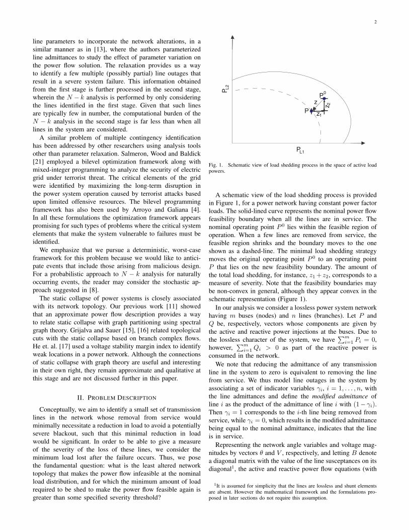
A schematic view of the load shedding process is providedin Figure 1, for a power network having constant power factorloads. The solid-lined curve represents the nominal power flowfeasibility boundary when all the lines are in service. Thenominal operating point P 0 lies within the feasible region ofoperation. When a few lines are removed from service, thefeasible region shrinks and the boundary moves to the oneshown as a dashed-line. The minimal load shedding strategymoves the original operating point P 0 to an operating pointP that lies on the new feasibility boundary. The amount ofthe total load shedding, for instance, z1 +z2, corresponds to ameasure of severity. Note that the feasibility boundaries maybe non-convex in general, although they appear convex in theschematic representation (Figure 1).

In our analysis we consider a lossless power system networkhaving m buses (nodes) and n lines (branches). Let P andQ be, respectively, vectors whose components are given bythe active and reactive power injections at the buses. Due tothe lossless character of the system, we have

∑mi=1 Pi = 0,

however,∑m

i=1 Qi > 0 as part of the reactive power isconsumed in the network.

We note that reducing the admittance of any transmissionline in the system to zero is equivalent to removing the linefrom service. We thus model line outages in the system byassociating a set of indicator variables γi, i = 1, . . . , n, withthe line admittances and define the modified admittance ofline i as the product of the admittance of line i with (1− γi).Then γi = 1 corresponds to the i-th line being removed fromservice, while γi = 0, which results in the modified admittancebeing equal to the nominal admittance, indicates that the lineis in service.

Representing the network angle variables and voltage mag-nitudes by vectors θ and V , respectively, and letting B denotea diagonal matrix with the value of the line susceptances on itsdiagonal1, the active and reactive power flow equations (with

1It is assumed for simplicity that the lines are lossless and shunt elementsare absent. However the mathematical framework and the formulations pro-posed in later sections do not require this assumption.

3

modified admittances) can be written in matrix form as

AT EB(I − Γ) sin(Aθ) = P (1)

−|A|T EB(I − Γ) cos(Aθ) + d = Q, (2)

where A is the branch-node incidence matrix of the networkgraph and |A|i,j = |Ai,j |, E is a diagonal matrix with

Ei,i = exp((|A| ln V )i), i = 1, . . . , n,

I is the identity matrix, Γ is a diagonal matrix with

Γi,i = γi, i = 1, . . . , n,

d is defined by

di = V 2i × (AT B(I − Γ)A)i,i, i = 1, . . . , m,

and sin(Aθ) denotes a vector whose i-th component is equalto sin((Aθ)i). Similar notation is used to define cos(Aθ) andln V . Refer to [22] for more details on this model.

Most work documented in the literature in this contextassumes the notion of a slack bus. The choice of the slackbus is typically arbitrary and it serves to supply networklosses. Moreover, in the event of load shedding or load pickup, the slack bus is assumed to provide the net reduction orincrement in the loads. It is well known, but often understated,that the results depend upon the choice of the slack bus.In this study, we use a distributed slack bus, where the netreduction in load due to load shedding is accounted for byevery generator in the system by lowering their respectivedispatches in proportion to their generating capacities. Thiseliminates the aspect of arbitrariness that the results containwhen a particular bus is used as a slack bus2. This choiceof distributed slack is motivated by the presence of droopgovernor controls on generators in which the response to adisturbance is distributed in a uniform manner among thegenerators. In the WECC system, for example, generators have5% droop governor controls [2].

We note that due to the incorporation of a single unifieddistributed slack mechanism in our framework, all the gen-erators in the system are redispatched in proportion to theirnominal dispatches in response to load shedding, even whenline failures result in system islanding (disconnected groupsor partitions). Multiple distributed slack mechanisms wouldbe more appropriate while dealing with cases when thereis partitioning of the graph underlying the system network.Such an approach can be easily followed once the partitioningdetails are known. However we note that the analysis presentedin this paper does not explicitly address issues related withsystem islanding and graph partitioning.

A. Power Flow Model, Load Shedding and Distributed Slack

Suppose that the system has mg PV (generator) buses andml PQ (load) buses, such that the total buses are m = mg+ml.Let P 0

pv and P 0pq be the vectors of active power injections at

PV and PQ buses, respectively, at the original operating pointP 0. Let z ∈ Rml be a vector representing a reduction in theactive load powers due to load shedding. In general, some

2The notion of a distributed slack is used in [7], [23] for other applications.

PQ buses in the network will not have any load connected tothem. In other words, such buses will have no load sheddingactivity associated with them. Corresponding components ofthe vector z are set to zero. It is assumed that the loads areconstant power factor loads, so that the relationship Q0

pq =MP 0

pq holds, where Q0pq represents a vector of reactive power

injections at PQ buses and M is a diagonal matrix. Hence, thereduction in reactive load powers is equal to Mz. In the spaceof active load powers, the vector z provides a direction for loadshedding, whose components are schematically represented inFigure 1.

Note that all the elements of z are nonnegative, whichis consistent with the sign convention (power injections arepositive) and that the loads are only allowed to be shed. Dueto the adopted notion of a distributed slack bus and the losslesscharacter of the network, the net reduction in the active powerload due to load shedding, i.e., eT z, where e = [1 1 . . . 1]T ∈Rml , is accounted for by a reduction in injection at everyPV bus in proportion to their nominal generation dispatch3.The net reduction in active power injections at PV buses isgiven by the product kP 0

pv , where k is a (nonpositive) scalar.It follows from the conservation of active power that we musthave eT z + keT P 0

pv = 0, therefore

k = − eT z

eT P 0pv

. (3)

Finally, we assume here that generator voltage controlsact to maintain voltage magnitudes at the PV buses at theirnominal values; one need only consider the reactive powerequations in (2) corresponding to PQ buses. Then, using (1)–(2), the power flow description at the new operating point Pthat is achieved after load shedding is given by

FPpv(θ, V, γ)− (

P 0pv + kP 0

pv

)= 0 (4)

FPpq(θ, V, γ)− (P 0

pq + z) = 0 (5)

FQpq(θ, V, γ)−M(P 0

pq + z) = 0, (6)

where k is as in (3), FPpv(θ, V, γ) and FP

pq(θ, V, γ) denote,respectively, the left-hand side from (1) corresponding to PVand PQ buses, and FQ

pq(θ, V, γ) represents the left-hand sidefrom (2) corresponding to PQ buses. For a given networktopology (i.e., for fixed γ), the system of equations (4)–(6) geometrically represents an ml-manifold in the space ofvariables (θ, V, z).

We remark that no active power balance equation is omittedin the power flow description (4)–(6), and thus no anglereference is provided. As a result, the power flow Jacobian

J =[

∂F∂θ

∂F∂V

](7)

has a trivial zero eigenvalue with w0 = [eT 0T ]T as thecorresponding left eigenvector, where e = [1 1 . . . 1]T ∈ Rm,w0 ∈ Rm+ml , and F denotes the left-hand side of (4)–(6).This is also apparent from the structure of (1)–(2) and thefact that the sum of the elements in each row of the incidence

3However, note that our approach is general enough to allow other distrib-uted slacks.

4

matrix A is equal to zero. Note that w0 satisfies

∂F

∂z

T

w0 = 0. (8)

B. Obtaining a (Locally) Best Load Shedding Strategy

Referring to Figure 1, a best load shedding strategy is soughtthat moves the initial operating point P 0 to a new operatingpoint P , such that a minimum amount of load is lost. Resultsin the literature related to this topic have employed a 2-norm notion of distance to a feasible operating point, see forexample [5]. In practice, since our emphasis is on minimumload shedding, it is more appropriate to express our distance ina 1-norm sense. That is, we are more interested in the simplesum of lost load than the sum of squared lost load.

Typically the 2-norm measure is more amenable to mathe-matical analysis than the 1-norm. The 1-norm measure intro-duces an aspect of non-smoothness in the analysis, and thusmay increase the complexity of the problem. As mentionedin Section II-A, in the present case however, note that everyload is only allowed to be shed as opposed to being increased.This requires all the elements of z to have the same sign, inparticular they need to be all nonnegative in the present frame-work. This observation greatly reduces the complexity thatthe problem would encounter otherwise, and simplifies ‖z‖1to eT z (which would otherwise be eT |z|). To determine sucha load shedding strategy, consider the following optimizationproblem,

minθ,V,z

eT z (9)

s.t. F (θ, V, z) = 0, (10)

P 0pq ≤ P 0

pq + z ≤ 0 (11)

Vmin ≤ V ≤ Vmax (12)−π/2 ≤ Aθ ≤ π/2 (13)

where (10) denotes the system (4)–(6) for a given networktopology (i.e., for fixed γ), such that it does not have asolution at z = 0. Inequality constraints (11)–(13) ensurethat the variables are within bounds. Note, in particular, that(11) ensures the validity of this formulation by enforcingnonnegativity of elements of vector z. It also ensures that theupper limit on the amount of load shedding is defined by thenominal load, thus preventing the loads to act as generators.Voltage magnitudes at PQ buses are bounded by upper andlower limits Vmax and Vmin, respectively, as indicated by (12).This constraint ensures that the voltages are within acceptablelimits, even after load shedding. With a good choice of Vmin,this constraint also serves to exclude low voltage (steadystate unstable) solutions from consideration. Constraint (13)guarantees that the phase angles across the transmission linesare in a range acceptable for a steady state stable operation ofthe power system.

The Lagrangian corresponding to (9)–(13) is

L = zT e + λT F (θ, V, z) + µT1 (−z) + µT

2 (P 0pq + z)

+ µT3 (Vmin − V ) + µT

4 (V − Vmax)

+ µT5 (−π/2−Aθ) + µT

6 (Aθ − π/2). (14)

where λ and µ1, . . . , µ6 are vectors of Lagrange multipli-ers. Optimal solutions to this problem satisfy the followingKarush-Kuhn-Tucker conditions,

e +∂F

∂z

T

λ− µ1 + µ2 = 0 (15)

JT λ +[ −AT µ5 + AT µ6

−µ3 + µ4

]= 0 (16)

µ1 · z = 0 (17)

µ2 · (P 0pq + z) = 0 (18)

µ3 · (Vmin − V ) = 0 (19)µ4 · (V − Vmax) = 0 (20)µ5 · (π/2 + Aθ) = 0 (21)µ6 · (Aθ − π/2) = 0 (22)

µ1, · · · , µ6 ≥ 0, (23)

along with (10)–(13). Thus the vector z that provides the bestload shedding strategy is obtained by solving (10) and (15)–(22), while honoring the inequalities (11)–(13) and (23). Thenotation “·” in (17)–(22) is used to indicate component-wisemultiplication of associated vectors.

When the inequality constraints (11)–(13) are inactive,we have µ1, . . . , µ6 = 0. Referring to (16), this results inJT λ = 0, which in turn makes λ a left eigenvector of Jcorresponding to its zero eigenvalue. Note that J must havean extra (nontrivial) zero eigenvalue as λ = w0 does not satisfy(15) and (8) simultaneously. In other words, λ equals w, wherew is a left eigenvector of J corresponding to its nontrivialzero eigenvalue. For this case, it is insightful to appreciate thegeometrical interpretation of (15)–(16). Consider a hyperplanetangent to the manifold defined by (10). Vectors (δθ, δV, δz)on that tangent hyperplane satisfy

J

[δθδV

]+

∂F

∂zδz = 0. (24)

Premultiplying with the eigenvector wT results in

wT J

[δθδV

]+ wT ∂F

∂z

T

δz = 0, (25)

However, as the first term in (25) vanishes to zero, we musthave

(∂F∂z w

)Tδz = 0. This implies that the normal to the

power flow feasibility boundary at (θ, V, z) is given by ∂F∂z

Tw.

It also follows from (15) that, this normal aligns with e whenthe inequality constraints are inactive.

C. Relaxation on Line Admittance Coefficients

Recall that our goal is to identify a small number oftransmission lines whose removal from service leads to asignificant system failure, where line outages are modeled viathe concept of modified admittance coefficients γ, as describedat the beginning of Section II. Realistically only two situationsare possible, namely, the i-th line is in service (γi = 0) orit is out of service (γi = 1). This introduces an aspect ofdiscreteness in the analysis framework and any optimizationproblem formulation that involves γi ∈ 0, 1 would result inan mixed-integer nonlinear programming problem. We note

5

that such problems are more difficult to handle than onesinvolving continuous variables.

We address this issue by relaxing the variable vector γ inthe first stage of our analysis, and allowing its elements totake continuous values between 0 and 1. In other words, weallow partial line outages by letting

γi ∈ [0, 1], i = 1, . . . , n. (26)

Note that the discussion on obtaining the best load sheddingstrategy as in Section II-B is applicable for any fixed networktopology (as long as the network remains connected). Thus itholds valid for situations when the lines are partially removedfrom service.

D. A Constrained Optimization Problem

To pose the contingency screening problem, the first stageof analysis uses a constrained optimization framework thatemploys the mechanisms of best load shedding strategy,distributed slack and partial line outages, described in theprevious sections. Note that we seek to move both the originaloperating point P 0 and the power flow feasibility boundary.This boundary is moved past P 0 such that the minimum loadshedding required to move P 0 to a different operating pointlying on the new boundary is greater than the minimum desiredseverity of the blackout. Mathematically, the problem takes thefollowing form,

minθ,V,z,γ,µ1,...,µ6,λ

eT γ (27)

s.t. F (θ, V, z, γ) = 0 (28)

e +∂F

∂z

T

λ− µ1 + µ2 = 0 (29)

JT λ +[ −AT µ5 + AT µ6

−µ3 + µ4

]= 0 (30)

µ1 · z = 0 (31)

µ2 · (P 0pq + z) = 0 (32)

µ3 · (Vmin − V ) = 0 (33)µ4 · (V − Vmax) = 0 (34)µ5 · (π/2 + Aθ) = 0 (35)µ6 · (Aθ − π/2) = 0 (36)

µ1, · · · , µ6 ≥ 0 (37)

P 0pq ≤ P 0

pq + z ≤ 0 (38)

Vmin ≤ V ≤ Vmax (39)−π/2 ≤ Aθ ≤ π/2 (40)

0 ≤ γ ≤ 1 (41)

eT z ≥ Smin. (42)

Constraints (28) denotes the power flow equations (10), nowwith γ as an additional variable. Together, constraints (28)–(40) are the Karush-Kuhn-Tucker conditions as obtained inSection II-B; they are repeated here for clarity. Constraint (41)follows from the relaxation on γ. Constraint (42) ensures thetotal amount of load shed is greater than Smin, a positive-valued user defined parameter that indicates the minimumdesired severity of the blackout.

By virtue of the distributed slack mechanism, all the gener-ators contribute to the load shedding in the same proportion.This ensures that all the generators must reduce (not increase)their dispatches to account for load shedding, thus in turnensuring that their upper dispatch capacity limits are not hit.This also guarantees that all generators will reach the lowerdispatching limit assumed as zero simultaneously, when allthe load in the system is shed. Thus a constraint that limitsgenerator dispatches is unnecessary and hence is not includedin the set of constraints (28)–(42).

In the present formulation, we aim to find the least numberof partial line outages that result in a failure having severitygreater than Smin. Another related formulation that can ad-dress our network vulnerability problem is where one aimsto find the maximum possible failure severity when at mostLmax number of lines are removed from service. Althoughboth these formulations carry the same conceptual flavor, theyare different problems depending upon the values that the userdefined parameters Smin and Lmax take. Mathematically, thelatter formulation has the same structure as (27)–(42), exceptthat the objective is now replaced by

maxθ,V,z,γ,µ1,...,µ6,λ

eT z, (43)

and the constraint (42) is replaced by

eT γ ≤ Lmax, (44)

while keeping other constraints intact.Using either formulation (27)–(42) or (43)–(44), the critical

lines for system security are identified as the ones that havenon-zero γ’s associated with them. In the second stage of ouranalysis, only such lines are considered for an N − k study,where N is the number of lines identified and k may takevalues from 1 through N .

III. EXAMPLES

To illustrate the application of the ideas discussed in Sec-tion II, we first consider a three bus system (Figure 2),followed by the IEEE 30 bus system (Figure 7).

A. Three Bus System

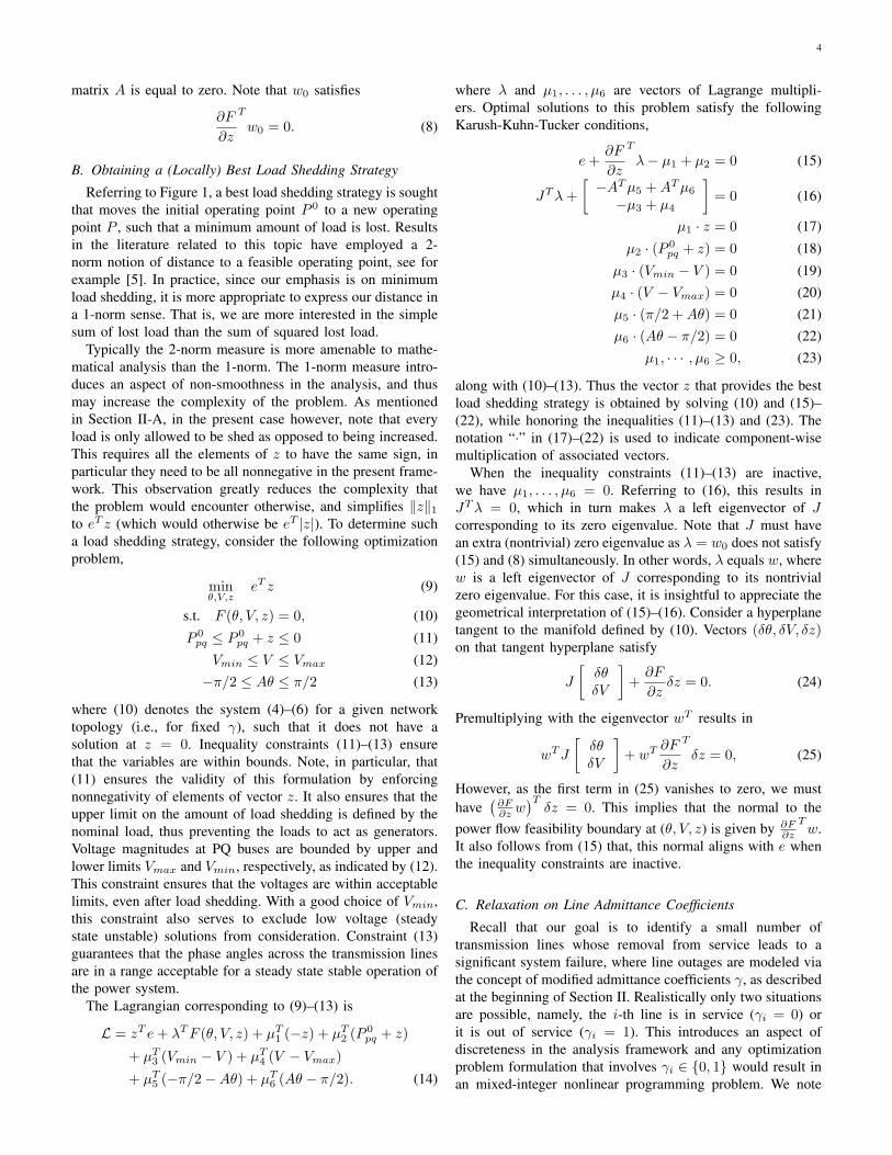
This small system is convenient for an easy graphicalvisualization of results and to highlight the main aspects ofour formulation. Consider the network as shown in Figure 2that has two generators and a single constant power factorload. The network data and the nominal power flow solutionare summarized in Table VI.

Figure 3 shows the space of active power injections atbuses 2 and 3. Given that the system is lossless, the powerinjection at bus 1 is simply −(P2 + P3) and considerationof another axis P1 is unnecessary. When all the lines arein service, the power flow solution space boundary can betraced by a continuation technique [18] and is identified asΣ0. The region enclosed by Σ0 contains all possible powerflow solutions that the present network topology (defined byline parameters) supports. The part of this region relevant tous is the quadrant having P2 ≥ 0 and P3 ≤ 0, given that

6

1

2

3

P1

P2

P3

=j0.1

X1

=j0.33X2

=j0.14X3

=j0

.33

X 4

=j0

.14

X 5

Fig. 2. Three bus system.

−20 −15 −10 −5 0 5 10 15 20−5

0

5

10

15

20

25

P2

P3

P0

P1

Σ0

Σ1

Fig. 3. Three bus system: nominal and modified power flow solution spaceboundary as defined by the solution in Table I.

the devices connected to buses 2 and 3 are a generator andload, respectively. Note that the nominal operating point P 0

lies within this region.Moreover, the subset of the power flow solution space that

contains solutions satisfying the voltage and angle constraints(39)–(40) defines the region of feasibility. At the nominaloperating point P 0, the load bus voltage is 0.84 p.u. The lowervoltage limit Vmin is set to 0.5 p.u. in the optimization formu-lation (discussed later). Generator buses 1 and 2 maintain theirvoltages at 1 p.u. Given that there are no shunt capacitors in thenetwork and line charging is ignored, the load bus 3 voltagewould not rise above 1 p.u., effectively making the constraintV ≤ Vmax unnecessary. The nominal operating point P 0 thuslies inside the region of feasibility.

Using the problem formulation (27)–(42), a few critical linesin this system are identified while ensuring that their removalwill cause a failure having a severity of at least 1 p.u., orequivalently the one that will necessitate at least 1 p.u. ofload shedding at bus 3. The corresponding parameter Smin isdefined as 1. The initial guess for the solution process wasobtained as described in Appendix II. The solution, summa-rized in Table I, identifies lines 3 and 5 as important. When

0 5 10 15 20−5

−4.5

−4

−3.5

−3

−2.5

−2

−1.5

−1

−0.5

0

P2

P3

P0

P1

Σ0

Σ1

Fig. 4. The fourth quadrant of Figure 3.

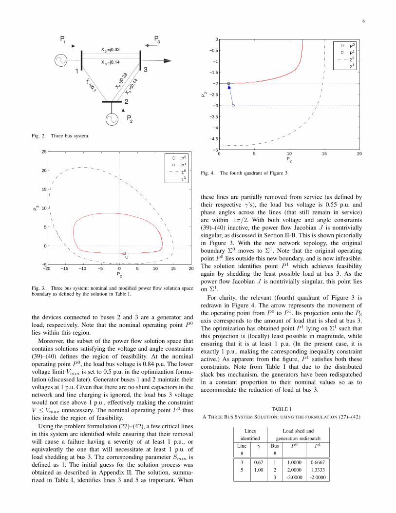
these lines are partially removed from service (as defined bytheir respective γ’s), the load bus voltage is 0.55 p.u. andphase angles across the lines (that still remain in service)are within ±π/2. With both voltage and angle constraints(39)–(40) inactive, the power flow Jacobian J is nontriviallysingular, as discussed in Section II-B. This is shown pictoriallyin Figure 3. With the new network topology, the originalboundary Σ0 moves to Σ1. Note that the original operatingpoint P 0 lies outside this new boundary, and is now infeasible.The solution identifies point P 1 which achieves feasibilityagain by shedding the least possible load at bus 3. As thepower flow Jacobian J is nontrivially singular, this point lieson Σ1.

For clarity, the relevant (fourth) quadrant of Figure 3 isredrawn in Figure 4. The arrow represents the movement ofthe operating point from P 0 to P 1. Its projection onto the P3

axis corresponds to the amount of load that is shed at bus 3.The optimization has obtained point P 1 lying on Σ1 such thatthis projection is (locally) least possible in magnitude, whileensuring that it is at least 1 p.u. (In the present case, it isexactly 1 p.u., making the corresponding inequality constraintactive.) As apparent from the figure, P 1 satisfies both theseconstraints. Note from Table I that due to the distributedslack bus mechanism, the generators have been redispatchedin a constant proportion to their nominal values so as toaccommodate the reduction of load at bus 3.

TABLE IA THREE BUS SYSTEM SOLUTION: USING THE FORMULATION (27)–(42)

Lines Load shed andidentified generation redispatch

Line γ Bus P 0 P 1

# #

3 0.67 1 1.0000 0.66675 1.00 2 2.0000 1.3333

3 -3.0000 -2.0000

7

0 5 10 15 20−5

−4.5

−4

−3.5

−3

−2.5

−2

−1.5

−1

−0.5

0

P2

P3

P0

P1

P2

Σ1

Σ0

Σ2

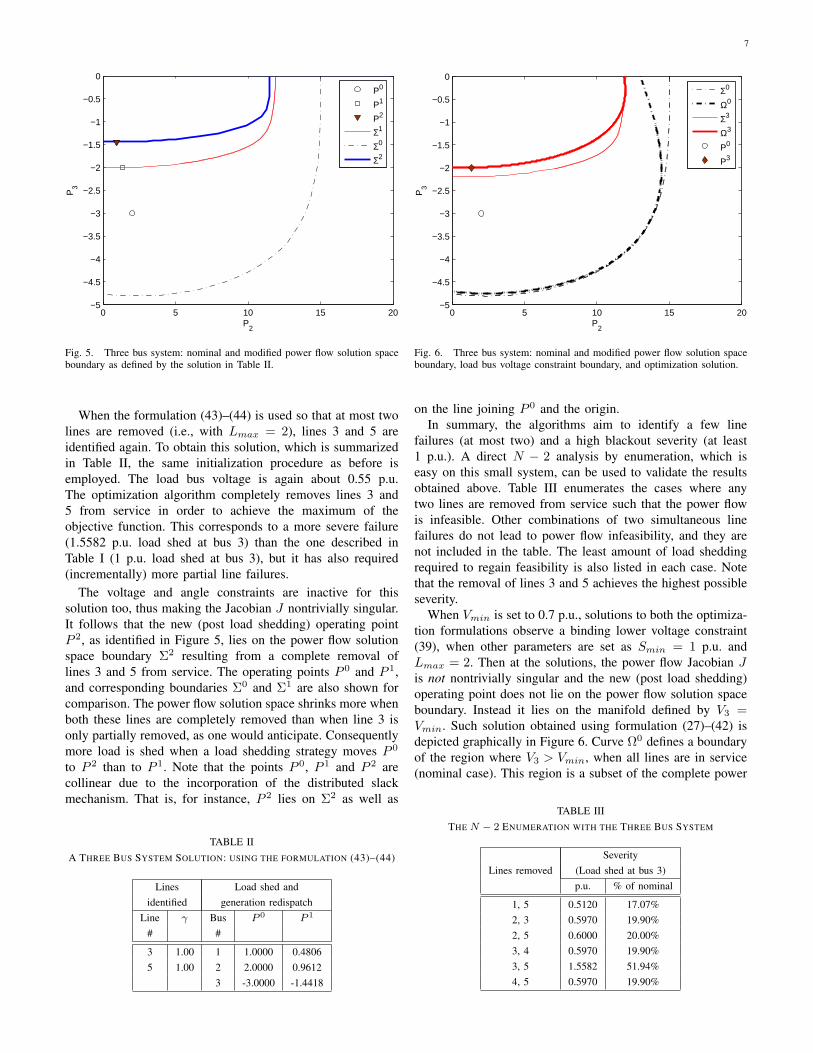
Fig. 5. Three bus system: nominal and modified power flow solution spaceboundary as defined by the solution in Table II.

When the formulation (43)–(44) is used so that at most twolines are removed (i.e., with Lmax = 2), lines 3 and 5 areidentified again. To obtain this solution, which is summarizedin Table II, the same initialization procedure as before isemployed. The load bus voltage is again about 0.55 p.u.The optimization algorithm completely removes lines 3 and5 from service in order to achieve the maximum of theobjective function. This corresponds to a more severe failure(1.5582 p.u. load shed at bus 3) than the one described inTable I (1 p.u. load shed at bus 3), but it has also required(incrementally) more partial line failures.

The voltage and angle constraints are inactive for thissolution too, thus making the Jacobian J nontrivially singular.It follows that the new (post load shedding) operating pointP 2, as identified in Figure 5, lies on the power flow solutionspace boundary Σ2 resulting from a complete removal oflines 3 and 5 from service. The operating points P 0 and P 1,and corresponding boundaries Σ0 and Σ1 are also shown forcomparison. The power flow solution space shrinks more whenboth these lines are completely removed than when line 3 isonly partially removed, as one would anticipate. Consequentlymore load is shed when a load shedding strategy moves P 0

to P 2 than to P 1. Note that the points P 0, P 1 and P 2 arecollinear due to the incorporation of the distributed slackmechanism. That is, for instance, P 2 lies on Σ2 as well as

TABLE IIA THREE BUS SYSTEM SOLUTION: USING THE FORMULATION (43)–(44)

Lines Load shed andidentified generation redispatch

Line γ Bus P 0 P 1

# #

3 1.00 1 1.0000 0.48065 1.00 2 2.0000 0.9612

3 -3.0000 -1.4418

0 5 10 15 20−5

−4.5

−4

−3.5

−3

−2.5

−2

−1.5

−1

−0.5

0

P2

P3

Σ0

Ω0

Σ3

Ω3

P0

P3

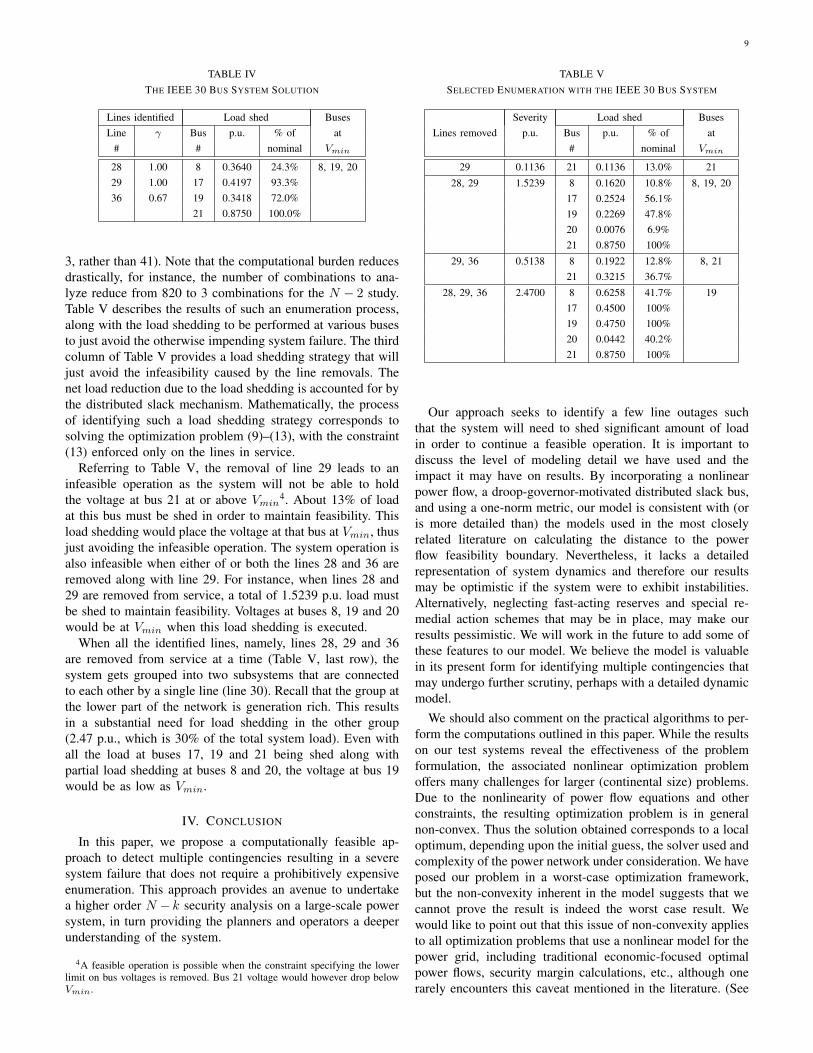
Fig. 6. Three bus system: nominal and modified power flow solution spaceboundary, load bus voltage constraint boundary, and optimization solution.

on the line joining P 0 and the origin.In summary, the algorithms aim to identify a few line

failures (at most two) and a high blackout severity (at least1 p.u.). A direct N − 2 analysis by enumeration, which iseasy on this small system, can be used to validate the resultsobtained above. Table III enumerates the cases where anytwo lines are removed from service such that the power flowis infeasible. Other combinations of two simultaneous linefailures do not lead to power flow infeasibility, and they arenot included in the table. The least amount of load sheddingrequired to regain feasibility is also listed in each case. Notethat the removal of lines 3 and 5 achieves the highest possibleseverity.

When Vmin is set to 0.7 p.u., solutions to both the optimiza-tion formulations observe a binding lower voltage constraint(39), when other parameters are set as Smin = 1 p.u. andLmax = 2. Then at the solutions, the power flow Jacobian Jis not nontrivially singular and the new (post load shedding)operating point does not lie on the power flow solution spaceboundary. Instead it lies on the manifold defined by V3 =Vmin. Such solution obtained using formulation (27)–(42) isdepicted graphically in Figure 6. Curve Ω0 defines a boundaryof the region where V3 > Vmin, when all lines are in service(nominal case). This region is a subset of the complete power

TABLE IIITHE N − 2 ENUMERATION WITH THE THREE BUS SYSTEM

SeverityLines removed (Load shed at bus 3)

p.u. % of nominal

1, 5 0.5120 17.07%2, 3 0.5970 19.90%2, 5 0.6000 20.00%3, 4 0.5970 19.90%3, 5 1.5582 51.94%4, 5 0.5970 19.90%

8

flow solution space, whose boundary is shown as Σ0. Theoptimization formulation identifies lines 3 and 5, with theirrelaxation parameters as γ3 = 0.55 and γ5 = 1. With theselines (partially) removed as defined by their respective γ’s,Σ0 moves to Σ3, and Ω0 to Ω3. The boundary Ω3 enclosessolutions having V3 > Vmin, at this network topology. Theoptimization identifies the new operating point P 3 that lies onΩ3, thus making sure that the voltage constraint is not violated,and yet at least 1 p.u. load is shed. In the present case, exactly1 p.u. load is shed.

We emphasize that due to the incorporation of voltage andangle constraints within our analysis, the solution feasibilityboundary that we seek is not always identical with the powerflow solution space boundary. It is the same as the power flowsolution space boundary when load voltages and line anglesare not at their limits. However, it is defined as the compositeboundary of the region Vmin ≤ Vl ≤ Vmax and −π/2 ≤θij ≤ +π/2, when load voltage(s) Vl or line angle(s) θij areat their limits. Mathematically, (30) defines such a feasibilityboundary.

In this three bus system, no single line failure contingencyresults in an infeasible operation. Thus the second stage ofN − k enumeration study involving only lines 3 and 5 isunnecessary. Finally, it is important to note that the schematicin Figure 1 shows a space of load powers while Figures 3, 4,5 and 6 show a complete space of all bus (nodal) powers. Asthere is only one load in the three bus system, the space of loadpowers is 1-dimensional and does not provide a significantvisualization aid.

B. IEEE 30 Bus System

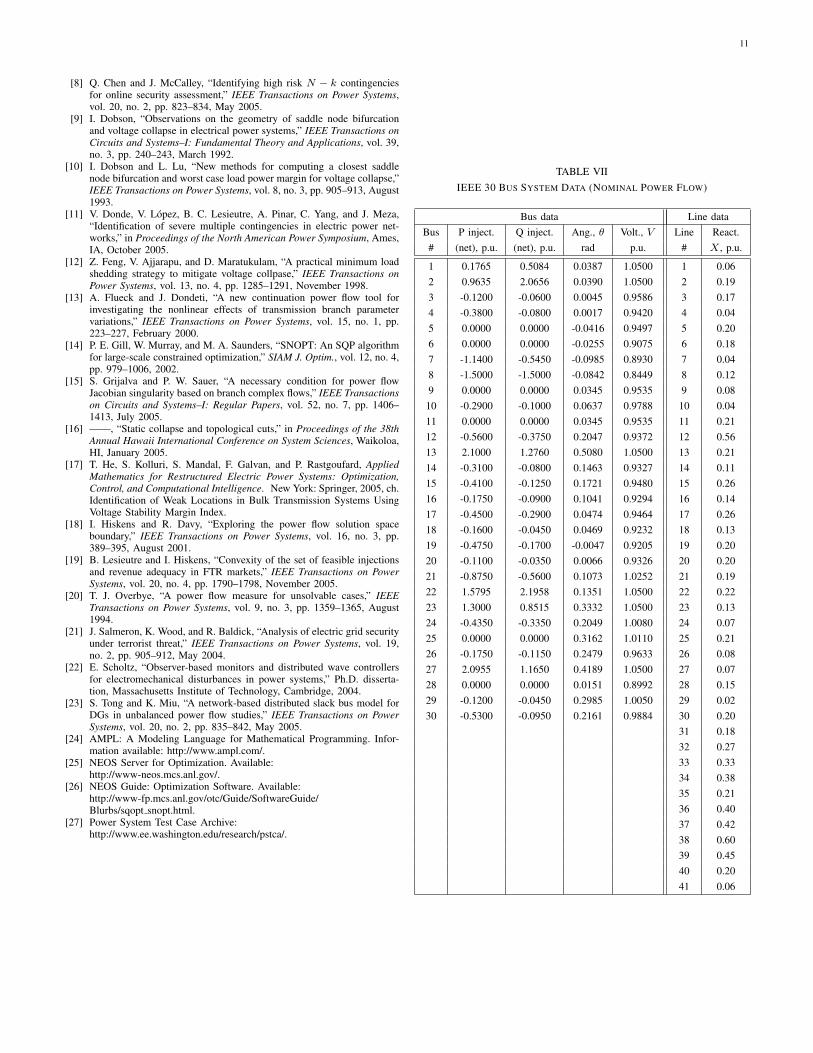
The IEEE 30 bus system as shown in Figure 7 is consideredfor the identification of lines critical for system security usingthe formulation discussed in Section II-D. The generators aredispatched in the original system data [27] in such a waythat the system observes an active power balance within theleft, right and the lower parts of the network. To emphasizesome important aspects of our algorithm, the generator activepower injections are modified so that there is no natural powerbalance in the system subsets. Table VII documents the systemdata that is used to obtain the results that follow.

Problem formulation (27)-(42) is used for the contingencyscreening. Feasible initial guesses were obtained according tothe procedure described in Appendix II. The solutions werecomputed using the solver SNOPT [14], the AMPL modelinglanguage [24], and the NEOS server for optimization [25],[26]. SNOPT uses a sequential quadratic programming algo-rithm suitable for problems with (nonlinear) objective functionand is designed for both nonlinear and linear constraints withsparse derivatives. The latter is particularly attractive for theoptimization problem under consideration.

An obvious (and trivial) solution to the optimization prob-lem is the one that isolates all the generation from the loads,by removing radial lines that connect generators (and/or loads)with rest of the system. Such cases are excluded by notallowing the radial lines (in this case, lines 13, 16 and 34) tobe removed from service, as our goal is to identify more subtle

1

67

5

4 3

2

119

828 16

2324

20

2122

302927

25

26 10

15

14

1213

1917

18

1

23

22

30

32

25

26

29

28

31

3937

38

3335

34

14

13

11

36

41

4010

7 15

98

65

3

4

2 20

16

18

24

19

17

21

lines partially removed

buses where someload is shed

buses at V

12

27

lines completely removed

min

Fig. 7. Optimization solution for the IEEE 30 bus system.

solutions, that is, those not trivially revealed in the networktopology.

Buses having generators attached to them are assumed tohave 1.05 p.u. voltage. The base case (all lines in service andno load shedding) power flow solution results in a voltageprofile such that the lowest bus voltage in the system is0.85 p.u (at bus 8). Within the optimization framework, thelimit of Vmin = 0.8 p.u. is enforced on load bus voltages.This places the nominal voltage profile within the rangeof allowable voltage magnitudes, thus making the nominaloperation feasible. Using the same argument as in Section III-A, we note that the constraint V ≤ Vmax is unnecessary forthis example.

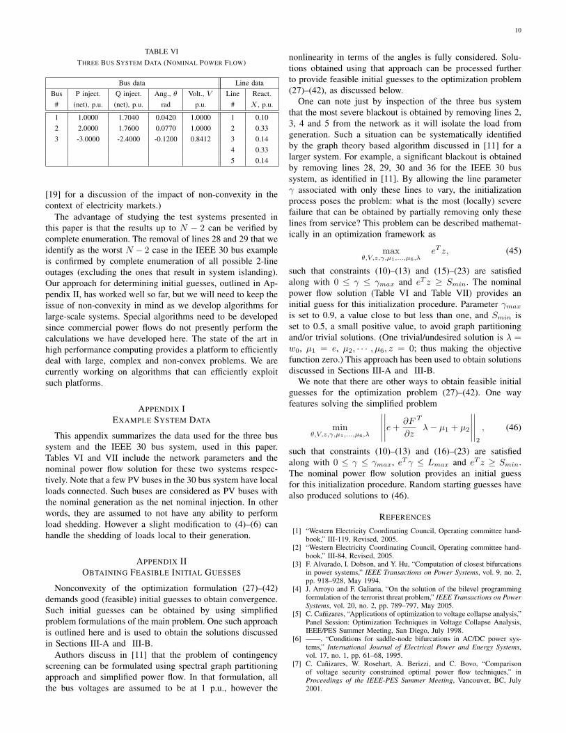
Figure 7 depicts a solution based upon an initial guess pro-vided by the initialization procedure described in Appendix II.The parameter Smin was set to 2 p.u. This solution identifiesthree transmission lines as critical ones. It also reveals thatthe aggregate of 2 p.u. load must be shed so as to just avoida failure when these lines are removed partially from service(as defined by their respective γ’s). This amounts to shedding24.4% of the total load in the system. Table IV summarizesthis solution. With lines 28 and 29 completely removed andline 36 partially removed from service, the generation richlower region of the network is almost unable to supply loads inthe other regions. This results in a sagging voltage at buses 19and 20, and they are constrained at Vmin. Effectively, as thesolution identifies, loads at this bus and neighboring busesmust be shed to maintain power flow and voltage feasibility.Recall that bus 8 had the lowest voltage at the base case powerflow. It turns out that some load must be shed at this bus too,in order to avoid the overall system failure, and its voltagewill sag down to Vmin post-load shedding.

Having identified the lines whose (even partial) failureresults in a severe system disturbance, one can perform theN −k study by only considering those lines (where N is now

9

TABLE IVTHE IEEE 30 BUS SYSTEM SOLUTION

Lines identified Load shed BusesLine γ Bus p.u. % of at

# # nominal Vmin

28 1.00 8 0.3640 24.3% 8, 19, 2029 1.00 17 0.4197 93.3%36 0.67 19 0.3418 72.0%

21 0.8750 100.0%

3, rather than 41). Note that the computational burden reducesdrastically, for instance, the number of combinations to ana-lyze reduce from 820 to 3 combinations for the N − 2 study.Table V describes the results of such an enumeration process,along with the load shedding to be performed at various busesto just avoid the otherwise impending system failure. The thirdcolumn of Table V provides a load shedding strategy that willjust avoid the infeasibility caused by the line removals. Thenet load reduction due to the load shedding is accounted for bythe distributed slack mechanism. Mathematically, the processof identifying such a load shedding strategy corresponds tosolving the optimization problem (9)–(13), with the constraint(13) enforced only on the lines in service.

Referring to Table V, the removal of line 29 leads to aninfeasible operation as the system will not be able to holdthe voltage at bus 21 at or above Vmin

4. About 13% of loadat this bus must be shed in order to maintain feasibility. Thisload shedding would place the voltage at that bus at Vmin, thusjust avoiding the infeasible operation. The system operation isalso infeasible when either of or both the lines 28 and 36 areremoved along with line 29. For instance, when lines 28 and29 are removed from service, a total of 1.5239 p.u. load mustbe shed to maintain feasibility. Voltages at buses 8, 19 and 20would be at Vmin when this load shedding is executed.

When all the identified lines, namely, lines 28, 29 and 36are removed from service at a time (Table V, last row), thesystem gets grouped into two subsystems that are connectedto each other by a single line (line 30). Recall that the group atthe lower part of the network is generation rich. This resultsin a substantial need for load shedding in the other group(2.47 p.u., which is 30% of the total system load). Even withall the load at buses 17, 19 and 21 being shed along withpartial load shedding at buses 8 and 20, the voltage at bus 19would be as low as Vmin.

IV. CONCLUSION

In this paper, we propose a computationally feasible ap-proach to detect multiple contingencies resulting in a severesystem failure that does not require a prohibitively expensiveenumeration. This approach provides an avenue to undertakea higher order N − k security analysis on a large-scale powersystem, in turn providing the planners and operators a deeperunderstanding of the system.

4A feasible operation is possible when the constraint specifying the lowerlimit on bus voltages is removed. Bus 21 voltage would however drop belowVmin.

TABLE VSELECTED ENUMERATION WITH THE IEEE 30 BUS SYSTEM

Severity Load shed BusesLines removed p.u. Bus p.u. % of at

# nominal Vmin

29 0.1136 21 0.1136 13.0% 21

28, 29 1.5239 8 0.1620 10.8% 8, 19, 2017 0.2524 56.1%19 0.2269 47.8%20 0.0076 6.9%21 0.8750 100%

29, 36 0.5138 8 0.1922 12.8% 8, 2121 0.3215 36.7%

28, 29, 36 2.4700 8 0.6258 41.7% 1917 0.4500 100%19 0.4750 100%20 0.0442 40.2%21 0.8750 100%

Our approach seeks to identify a few line outages suchthat the system will need to shed significant amount of loadin order to continue a feasible operation. It is important todiscuss the level of modeling detail we have used and theimpact it may have on results. By incorporating a nonlinearpower flow, a droop-governor-motivated distributed slack bus,and using a one-norm metric, our model is consistent with (oris more detailed than) the models used in the most closelyrelated literature on calculating the distance to the powerflow feasibility boundary. Nevertheless, it lacks a detailedrepresentation of system dynamics and therefore our resultsmay be optimistic if the system were to exhibit instabilities.Alternatively, neglecting fast-acting reserves and special re-medial action schemes that may be in place, may make ourresults pessimistic. We will work in the future to add some ofthese features to our model. We believe the model is valuablein its present form for identifying multiple contingencies thatmay undergo further scrutiny, perhaps with a detailed dynamicmodel.

We should also comment on the practical algorithms to per-form the computations outlined in this paper. While the resultson our test systems reveal the effectiveness of the problemformulation, the associated nonlinear optimization problemoffers many challenges for larger (continental size) problems.Due to the nonlinearity of power flow equations and otherconstraints, the resulting optimization problem is in generalnon-convex. Thus the solution obtained corresponds to a localoptimum, depending upon the initial guess, the solver used andcomplexity of the power network under consideration. We haveposed our problem in a worst-case optimization framework,but the non-convexity inherent in the model suggests that wecannot prove the result is indeed the worst case result. Wewould like to point out that this issue of non-convexity appliesto all optimization problems that use a nonlinear model for thepower grid, including traditional economic-focused optimalpower flows, security margin calculations, etc., although onerarely encounters this caveat mentioned in the literature. (See

10

TABLE VITHREE BUS SYSTEM DATA (NOMINAL POWER FLOW)

Bus data Line dataBus P inject. Q inject. Ang., θ Volt., V Line React.

# (net), p.u. (net), p.u. rad p.u. # X , p.u.

1 1.0000 1.7040 0.0420 1.0000 1 0.102 2.0000 1.7600 0.0770 1.0000 2 0.333 -3.0000 -2.4000 -0.1200 0.8412 3 0.14

4 0.335 0.14

[19] for a discussion of the impact of non-convexity in thecontext of electricity markets.)

The advantage of studying the test systems presented inthis paper is that the results up to N − 2 can be verified bycomplete enumeration. The removal of lines 28 and 29 that weidentify as the worst N − 2 case in the IEEE 30 bus exampleis confirmed by complete enumeration of all possible 2-lineoutages (excluding the ones that result in system islanding).Our approach for determining initial guesses, outlined in Ap-pendix II, has worked well so far, but we will need to keep theissue of non-convexity in mind as we develop algorithms forlarge-scale systems. Special algorithms need to be developedsince commercial power flows do not presently perform thecalculations we have developed here. The state of the art inhigh performance computing provides a platform to efficientlydeal with large, complex and non-convex problems. We arecurrently working on algorithms that can efficiently exploitsuch platforms.

APPENDIX IEXAMPLE SYSTEM DATA

This appendix summarizes the data used for the three bussystem and the IEEE 30 bus system, used in this paper.Tables VI and VII include the network parameters and thenominal power flow solution for these two systems respec-tively. Note that a few PV buses in the 30 bus system have localloads connected. Such buses are considered as PV buses withthe nominal generation as the net nominal injection. In otherwords, they are assumed to not have any ability to performload shedding. However a slight modification to (4)–(6) canhandle the shedding of loads local to their generation.

APPENDIX IIOBTAINING FEASIBLE INITIAL GUESSES

Nonconvexity of the optimization formulation (27)–(42)demands good (feasible) initial guesses to obtain convergence.Such initial guesses can be obtained by using simplifiedproblem formulations of the main problem. One such approachis outlined here and is used to obtain the solutions discussedin Sections III-A and III-B.

Authors discuss in [11] that the problem of contingencyscreening can be formulated using spectral graph partitioningapproach and simplified power flow. In that formulation, allthe bus voltages are assumed to be at 1 p.u., however the

nonlinearity in terms of the angles is fully considered. Solu-tions obtained using that approach can be processed furtherto provide feasible initial guesses to the optimization problem(27)–(42), as discussed below.

One can note just by inspection of the three bus systemthat the most severe blackout is obtained by removing lines 2,3, 4 and 5 from the network as it will isolate the load fromgeneration. Such a situation can be systematically identifiedby the graph theory based algorithm discussed in [11] for alarger system. For example, a significant blackout is obtainedby removing lines 28, 29, 30 and 36 for the IEEE 30 bussystem, as identified in [11]. By allowing the line parameterγ associated with only these lines to vary, the initializationprocess poses the problem: what is the most (locally) severefailure that can be obtained by partially removing only theselines from service? This problem can be described mathemat-ically in an optimization framework as

maxθ,V,z,γ,µ1,...,µ6,λ

eT z, (45)

such that constraints (10)–(13) and (15)–(23) are satisfiedalong with 0 ≤ γ ≤ γmax and eT z ≥ Smin. The nominalpower flow solution (Table VI and Table VII) provides aninitial guess for this initialization procedure. Parameter γmax

is set to 0.9, a value close to but less than one, and Smin isset to 0.5, a small positive value, to avoid graph partitioningand/or trivial solutions. (One trivial/undesired solution is λ =w0, µ1 = e, µ2, · · · , µ6, z = 0; thus making the objectivefunction zero.) This approach has been used to obtain solutionsdiscussed in Sections III-A and III-B.

We note that there are other ways to obtain feasible initialguesses for the optimization problem (27)–(42). One wayfeatures solving the simplified problem

minθ,V,z,γ,µ1,...,µ6,λ

∣∣∣∣∣

∣∣∣∣∣e +∂F

∂z

T

λ− µ1 + µ2

∣∣∣∣∣

∣∣∣∣∣2

, (46)

such that constraints (10)–(13) and (16)–(23) are satisfiedalong with 0 ≤ γ ≤ γmax, eT γ ≤ Lmax and eT z ≥ Smin.The nominal power flow solution provides an initial guessfor this initialization procedure. Random starting guesses havealso produced solutions to (46).

REFERENCES

[1] “Western Electricity Coordinating Council, Operating committee hand-book,” III-119, Revised, 2005.

[2] “Western Electricity Coordinating Council, Operating committee hand-book,” III-84, Revised, 2005.

[3] F. Alvarado, I. Dobson, and Y. Hu, “Computation of closest bifurcationsin power systems,” IEEE Transactions on Power Systems, vol. 9, no. 2,pp. 918–928, May 1994.

[4] J. Arroyo and F. Galiana, “On the solution of the bilevel programmingformulation of the terrorist threat problem,” IEEE Transactions on PowerSystems, vol. 20, no. 2, pp. 789–797, May 2005.

[5] C. Canizares, “Applications of optimization to voltage collapse analysis,”Panel Session: Optimization Techniques in Voltage Collapse Analysis,IEEE/PES Summer Meeting, San Diego, July 1998.

[6] ——, “Conditions for saddle-node bifurcations in AC/DC power sys-tems,” International Journal of Electrical Power and Energy Systems,vol. 17, no. 1, pp. 61–68, 1995.

[7] C. Canizares, W. Rosehart, A. Berizzi, and C. Bovo, “Comparisonof voltage security constrained optimal power flow techniques,” inProceedings of the IEEE-PES Summer Meeting, Vancouver, BC, July2001.

11

[8] Q. Chen and J. McCalley, “Identifying high risk N − k contingenciesfor online security assessment,” IEEE Transactions on Power Systems,vol. 20, no. 2, pp. 823–834, May 2005.

[9] I. Dobson, “Observations on the geometry of saddle node bifurcationand voltage collapse in electrical power systems,” IEEE Transactions onCircuits and Systems–I: Fundamental Theory and Applications, vol. 39,no. 3, pp. 240–243, March 1992.

[10] I. Dobson and L. Lu, “New methods for computing a closest saddlenode bifurcation and worst case load power margin for voltage collapse,”IEEE Transactions on Power Systems, vol. 8, no. 3, pp. 905–913, August1993.

[11] V. Donde, V. Lopez, B. C. Lesieutre, A. Pinar, C. Yang, and J. Meza,“Identification of severe multiple contingencies in electric power net-works,” in Proceedings of the North American Power Symposium, Ames,IA, October 2005.

[12] Z. Feng, V. Ajjarapu, and D. Maratukulam, “A practical minimum loadshedding strategy to mitigate voltage collpase,” IEEE Transactions onPower Systems, vol. 13, no. 4, pp. 1285–1291, November 1998.

[13] A. Flueck and J. Dondeti, “A new continuation power flow tool forinvestigating the nonlinear effects of transmission branch parametervariations,” IEEE Transactions on Power Systems, vol. 15, no. 1, pp.223–227, February 2000.

[14] P. E. Gill, W. Murray, and M. A. Saunders, “SNOPT: An SQP algorithmfor large-scale constrained optimization,” SIAM J. Optim., vol. 12, no. 4,pp. 979–1006, 2002.

[15] S. Grijalva and P. W. Sauer, “A necessary condition for power flowJacobian singularity based on branch complex flows,” IEEE Transactionson Circuits and Systems–I: Regular Papers, vol. 52, no. 7, pp. 1406–1413, July 2005.

[16] ——, “Static collapse and topological cuts,” in Proceedings of the 38thAnnual Hawaii International Conference on System Sciences, Waikoloa,HI, January 2005.

[17] T. He, S. Kolluri, S. Mandal, F. Galvan, and P. Rastgoufard, AppliedMathematics for Restructured Electric Power Systems: Optimization,Control, and Computational Intelligence. New York: Springer, 2005, ch.Identification of Weak Locations in Bulk Transmission Systems UsingVoltage Stability Margin Index.

[18] I. Hiskens and R. Davy, “Exploring the power flow solution spaceboundary,” IEEE Transactions on Power Systems, vol. 16, no. 3, pp.389–395, August 2001.

[19] B. Lesieutre and I. Hiskens, “Convexity of the set of feasible injectionsand revenue adequacy in FTR markets,” IEEE Transactions on PowerSystems, vol. 20, no. 4, pp. 1790–1798, November 2005.

[20] T. J. Overbye, “A power flow measure for unsolvable cases,” IEEETransactions on Power Systems, vol. 9, no. 3, pp. 1359–1365, August1994.

[21] J. Salmeron, K. Wood, and R. Baldick, “Analysis of electric grid securityunder terrorist threat,” IEEE Transactions on Power Systems, vol. 19,no. 2, pp. 905–912, May 2004.

[22] E. Scholtz, “Observer-based monitors and distributed wave controllersfor electromechanical disturbances in power systems,” Ph.D. disserta-tion, Massachusetts Institute of Technology, Cambridge, 2004.

[23] S. Tong and K. Miu, “A network-based distributed slack bus model forDGs in unbalanced power flow studies,” IEEE Transactions on PowerSystems, vol. 20, no. 2, pp. 835–842, May 2005.

[24] AMPL: A Modeling Language for Mathematical Programming. Infor-mation available: http://www.ampl.com/.

[25] NEOS Server for Optimization. Available:http://www-neos.mcs.anl.gov/.

[26] NEOS Guide: Optimization Software. Available:http://www-fp.mcs.anl.gov/otc/Guide/SoftwareGuide/Blurbs/sqopt snopt.html.

[27] Power System Test Case Archive:http://www.ee.washington.edu/research/pstca/.

TABLE VIIIEEE 30 BUS SYSTEM DATA (NOMINAL POWER FLOW)

Bus data Line dataBus P inject. Q inject. Ang., θ Volt., V Line React.

# (net), p.u. (net), p.u. rad p.u. # X , p.u.

1 0.1765 0.5084 0.0387 1.0500 1 0.062 0.9635 2.0656 0.0390 1.0500 2 0.193 -0.1200 -0.0600 0.0045 0.9586 3 0.174 -0.3800 -0.0800 0.0017 0.9420 4 0.045 0.0000 0.0000 -0.0416 0.9497 5 0.206 0.0000 0.0000 -0.0255 0.9075 6 0.187 -1.1400 -0.5450 -0.0985 0.8930 7 0.048 -1.5000 -1.5000 -0.0842 0.8449 8 0.129 0.0000 0.0000 0.0345 0.9535 9 0.0810 -0.2900 -0.1000 0.0637 0.9788 10 0.0411 0.0000 0.0000 0.0345 0.9535 11 0.2112 -0.5600 -0.3750 0.2047 0.9372 12 0.5613 2.1000 1.2760 0.5080 1.0500 13 0.2114 -0.3100 -0.0800 0.1463 0.9327 14 0.1115 -0.4100 -0.1250 0.1721 0.9480 15 0.2616 -0.1750 -0.0900 0.1041 0.9294 16 0.1417 -0.4500 -0.2900 0.0474 0.9464 17 0.2618 -0.1600 -0.0450 0.0469 0.9232 18 0.1319 -0.4750 -0.1700 -0.0047 0.9205 19 0.2020 -0.1100 -0.0350 0.0066 0.9326 20 0.2021 -0.8750 -0.5600 0.1073 1.0252 21 0.1922 1.5795 2.1958 0.1351 1.0500 22 0.2223 1.3000 0.8515 0.3332 1.0500 23 0.1324 -0.4350 -0.3350 0.2049 1.0080 24 0.0725 0.0000 0.0000 0.3162 1.0110 25 0.2126 -0.1750 -0.1150 0.2479 0.9633 26 0.0827 2.0955 1.1650 0.4189 1.0500 27 0.0728 0.0000 0.0000 0.0151 0.8992 28 0.1529 -0.1200 -0.0450 0.2985 1.0050 29 0.0230 -0.5300 -0.0950 0.2161 0.9884 30 0.20

31 0.1832 0.2733 0.3334 0.3835 0.2136 0.4037 0.4238 0.6039 0.4540 0.2041 0.06