DECEMBER 2000 507B E T T S

q 2000 American Meteorological Society

Idealized Model for Equilibrium Boundary Layer over Land

ALAN K. BETTS

Atmospheric Research, Pittsford, Vermont

(Manuscript received 24 January 2000, in final form 10 July 2000)

ABSTRACT

An idealized equilibrium mixed layer (ML) model is used to explore the coupling between the surface, theML, and the atmosphere above. It shows that ML depth increases as vegetative resistance to evaporation increases.The surface radiative forcing also increases ML depth; the ML radiative and evaporative cooling processesreduce ML depth. The model largely uncouples mean ML structure from the mean ML fluxes. The upper boundarycondition controls ML potential temperature and mixing ratio but does not affect the fluxes; it is the surfaceradiative forcing and the radiative and evaporative cooling terms within the ML (together with the vegetativeresistance Ry ) that control the surface fluxes and evaporative fraction. Furthermore, for a given Ry , the radiativeand evaporative cooling terms in the ML control the surface sensible heat flux, and the surface radiative forcingthen controls the surface latent heat flux. The solutions show that, except for extreme high values of vegetativeresistance and very dry air above the ML, this idealized equilibrium ML is capped by shallow cumulus clouds,as over the ocean. At the same time as Ry increases, the ML structure and depth shift from the oceanic limittoward a warmer, drier boundary layer. It is shown that surface evaporation controls equilibrium near-surfacerelative humidity and not vice versa. The equilibrium solutions also give insight into how the gradient of meanmixing ratio across the Mississippi River basin is linked to changes in surface pressure as well as vegetativeresistance to evaporation. The equilibrium model is oversimplified, and the nonlinearities introduced by thediurnal cycle have not been addressed, but nonetheless the solutions are a plausible zero-order fit to daily meanmodel data for the Missouri and Arkansas–Red River basins and to summer composites from the First InternationalLand-Surface Climatology Project Field Experiment.

1. Introduction

Understanding the surface climate equilibrium overland is important, if we are to assess the feedbacks as-sociated with climate change. The land and ocean sur-faces differ in two important ways. Water is not freelyavailable for evaporation over land. In simple land sur-face models this is usually represented using an extraresistance to evaporation. In addition, the effective ther-mal capacity of the land surface is much smaller thanthe ocean mixed layer, so that there is a much largerdiurnal cycle of temperature over land, driven by thediurnal cycle of the solar forcing at the surface. Froma modeling perspective it is also significant that, unlikesea surface temperature (SST), maps of the land surfacetemperature (which is more heterogeneous than theocean SST) are not routinely produced, and the avail-ability of water for evaporation is not readily observed.As a result, in global and regional forecast models (inaddition to climate models), all the fluxes and variablesat the land surface are currently calculated. In contrast,

Corresponding author address: Alan K. Betts, Atmospheric Re-search, 58 Hendee Lane, Pittsford, VT 05763.E-mail: akbetts@aol.com

in short- to medium-range forecast models, the oceansurface temperature is specified as an initial condition,and, in seasonal forecasting and climate modeling, theocean boundary condition, like that over land, is alsosolved as a coupled problem. All forecast and climatemodels drift to their own ‘‘model climate,’’ and, if wecan understand by using a simple model how the equi-librium climate at the land surface is determined (ontimescales longer than the diurnal) by the coupling ofthe model physical parameterizations, then we can moreeasily correct the systematic biases of the model. Overthe ocean, considerable progress has been made in un-derstanding the surface and boundary layer (BL) equi-librium climate, especially in the Tropics, using simplebulk models such as those of Sarachik (1978), Betts andRidgway (1988, 1989, 1992), Pierrehumbert (1995), andClement and Seager (1999). The purpose of this paperis to address in part the analogous surface climate equi-librium over land for the midcontinental summer BL,which has received much less attention.

The simplification that will be made is to averageover the diurnal cycle and to explore the interrelationof diurnally averaged state variables and fluxes, focus-ing primarily on the links to availability of water forevaporation. The analysis tool for understanding the dai-ly average surface climate is a mixed boundary layer

508 VOLUME 1J O U R N A L O F H Y D R O M E T E O R O L O G Y

model. The mixed layer (ML) model has a long history,having been used for stratocumulus BLs by Lilly (1968)and for the dry BL by Betts (1973), Carson (1973), andTennekes (1973). It will not, however, be used (as it isoften is) to represent the growth of the daytime mixedlayer driven by solar heating. Instead it will be used torepresent a hypothetical daily average equilibrium ML,driven by the daily average surface net radiation budgetand boundary conditions above the mixed layer. Thisapproach needs further explanation. The diurnal cycleover land involves nonlinear processes at the surface,where the daytime BL is unstable and relatively wellmixed and the nocturnal BL is strongly stable. Effectivesurface transfer coefficients are very different betweenday and night. It may seem surprising that an equilib-rium model, which ignores this complexity in the diurnalcycle, could be of any value in understanding the dailyaverage surface state. However, the motivation camefrom noticing the high level of structure in EuropeanCentre for Medium-Range Weather Forecasts(ECMWF) reanalysis daily average data, in relation tosoil moisture, which invited a simple theoretical expla-nation. There is no doubt that more detailed studies withdiurnally varying models will refine the details of thepicture, but one intent of this paper is to show that thebasic coupling of the surface thermodynamic variablesand fluxes can be interpreted with a very simple equi-librium model. A second intent is to focus attention onthe importance of explaining the mean diurnal state (andits longer timescale evolution), which is usually ignoredby studies of the diurnal evolution of the BL (which aretypically initialized with a morning BL state near sun-rise).

I will first show the theoretical solutions of the equi-librium mixed layer model and then use two sets of datafor illustration. One set is from the ECMWF reanalysisfor the nine Julys from 1985 to 1993, averaged for theRed–Arkansas and Missouri River basins. This datasetwas analyzed from an energy and hydrological per-spective in Betts et al. (1998, 1999a). Although thesedata are purely model derived, they have the advantageof being extensive and complete, with a variable setcoupled by the known model physical parameterizations(which may of course have formulation errors). A sec-ond, much smaller dataset (from Betts and Ball 1998)is the First International Land Surface Climatology Pro-ject Field Experiment (FIFE) data for the compositediurnal cycle for sets of days without rain in midsummer.This is a more limited dataset, covering only 53 daysand representative of only a 15 km 3 15 km area, butit has the advantage, of course, that it was derived fromreal observations. Last, the same data will be used toillustrate the relationship between the availability of soilwater, diurnal averages, and the diurnal cycle of thesurface lifting condensation level.

The observational studies of Betts and Ball (1995,1998) and Betts et al. (1999b), as well as the studieswith model data of Betts et al. (1998, 1999a), have

shown the strong link between the availability of waterfor evaporation and the pressure height of the liftingcondensation level or saturation level, or conversely thesurface relative humidity, both in the daily average andin the daytime diurnal cycle. Heuristically, the drop ofthe mean saturation at the surface, between, for example,the saturation inside and the subsaturation outside a leafsurface, is clearly linked directly to the constraints onwater evaporation. Indeed, this is one key differencebetween land and ocean. However, the low thermal ca-pacity of the land surface means that the equilibriumtemperature and humidity are tightly coupled. The ide-alized equilibrium solutions will show the dependenceof all the thermodynamic variables (surface temperature,potential temperature, equivalent potential temperature,relative humidity, and saturation level) on the avail-ability of water for evaporation and on thermodynamicparameters above the mixed layer. The analysis willilluminate how the mean surface energy partition (con-trolled by the availability of water for evaporation) con-trols the daily equilibrium temperature and humidity.

In a wider context, many papers have addressed thesurface boundary condition over land and its effect onatmospheric circulations. Schar et al. (1999) discussedthe soil moisture–precipitation feedback using a re-gional climate model over Europe and found their re-sults were consistent with the earlier studies of Beljaarset al. (1996), Betts et al. (1996), and Eltahir (1998) inthat high evaporation from wet soils led to a low Bowenratio and low BL height. De Ridder (1997) used an MLmodel of the daytime BL to show that lower Bowenratio led to higher equivalent potential temperature. Ina later paper, De Ridder (1998) integrated a 1D modelover a month of diurnal cycles to show the link betweensoil water surface evaporation and BL properties. How-ever, the long-term equilibrium was controlled by re-laxation terms. The model solutions shown in the nextsection directly address this long-term equilibrium byaveraging over the diurnal cycle.

2. Idealized steady-state mixed layer model

The model is really a ‘‘toy’’ model for a hypotheticalsteady-state mixed layer over land. Bulk aerodynamicequations at the surface are coupled to an extension ofthe classic mixed layer model (Betts 1973; Carson 1973;Tennekes 1973). The surface forcing is the daily averagenet radiation, and the availability of water for evapo-ration at the surface is represented by a bulk vegetativeresistance. Within the mixed layer, two diabatic pro-cesses are represented, radiative cooling and an evap-oration of falling precipitation, which cools and moist-ens the mixed layer while conserving its equivalent po-tential temperature. A specified potential temperaturegradient and saturation pressure difference [closely re-lated to relative humidity (RH)] give the upper boundarycondition for the mixed layer. Fluxes out of the mixedlayer into ‘‘clouds’’ are represented by a vertical mass

DECEMBER 2000 509B E T T S

flux, which is determined in equilibrium by imposingthe constraint that the lifting condensation level (LCL),representing cloud base, equal the mixed layer depth.The model solutions are consistent with a positive cloudmass flux.

How does this toy equilibrium model relate to themean diurnal cycle over land? During the daytime, thesurface fluxes are large and the ML grows rapidly, brief-ly reaching a quasi equilibrium in the afternoon beforecollapsing at sunset. During the daytime, the BL growthis generally much larger than the mean subsidence,which is closely related in the mean to the radiativecooling as over the oceans (Betts and Ridgway 1988,1989). Typically over land, a shallow cumulus layerforms at the top of the mixed layer, so that during mostof the daytime hours, mixed layer depth and cloud-baseheight are tightly coupled. This convective flux out ofthe mixed layer into clouds is a more important con-straint on daytime ML growth than is the mean subsi-dence. At night, the surface cools faster than the ML;a stable BL forms and grows during the night, influencedby radiative cooling, subsidence, and surface fluxes. Thesurface uncouples from the atmosphere and shallowclouds dissipate. What determines the long-term equi-librium, if conditions were the same day after day? Inthe thermal balance, there is a net upward surface sen-sible heat flux and a subsidence warming, which bal-ances the net radiative cooling and, on some days, evap-orative cooling of falling precipitation. In the moisturebalance, a net upward latent heat flux balances a dryingby subsidence, offset on some days again by the evap-oration of falling precipitation. Diurnally integrated,these balances are similar over land as over the ocean,and we will use similar closures. The difference overland is that the surface fluxes are much larger in thedaytime, when they are driven by the surface net ra-diation balance, and a mixed layer is generated withupward fluxes through cloud base; the fluxes are smallerat night. The steady-state solution, which averages overthe stable and unstable BLs, is clearly not at all satis-factory in a quantitative sense, because, for example,representative surface transfer coefficients are hard todefine, but the solutions are valuable qualitatively, be-cause over the diurnal cycle the primary balances arebetween surface fluxes, radiation, and subsidence (andon some days the evaporation of precipitation).

a. Surface fluxes

The sensible (SH) and latent (LH) heat fluxes at thesurface are driven by the net available energy Q*, whichwill be specified. The balance can be written

Q* 5 Rnet 2 G 5 SH 1 LH, (1)

where Rnet and G are the diurnally averaged net radiationand ground heat fluxes (G will typically be small). Theequations for the SH and LH fluxes can be written,following Monteith (1981), with u0 as a surface (aero-

dynamic) potential temperature (I shall ignore the dif-ference between a surface sensible heat flux and a po-tential heat flux), as

SH 5 C F 5 rC g (u 2 u ), (2a)p 0u p a 0 M

LH 5 LF 5 rLg (q 2 q ) 5 rLg [q (T ) 2 q ]0q a 0 M y s0 0 0

g gy a5 rL [q (T ) 2 q ], (2b)s0 0 M1 2g 1 ga y

where r and Cp are the density and heat capacity of air ;L is the latent heat of evaporation; F0u and F0q are thesurface fluxes of potential temperature and moisture; uM

and qM are the potential temperature and specific hu-midity in the mixed layer; T0, q0, and qs0 are, respec-tively, the temperature, specific humidity, and saturationspecific humidity at the surface; ga is an aerodynamicconductance; and gy is a vegetative conductance. As inthe original Penman–Monteith solutions, given Q* andthe surface transfer coefficients, the surface temperaturecan be eliminated from (1) and (2), and the surfacefluxes are then linked to the mixed layer solution foruM and qM. The aerodynamic conductance will be nom-inally defined as

ga 5 CTVs, (3)

with a constant transfer coefficient CT 5 1022 (i.e., weneglect dependence on stability) and a constant meanwind speed of Vs 5 2.5 m s21 to give ga 5 0.025 ms21. The vegetative conductance is related to a vege-tative resistance Ry by

gy 5 1/Ry . (4)

This resistance is the parameter that controls the avail-ability of water for evaporation at the surface and willbe specified with the range from 60 to 900 s m21, rep-resentative of the range from well-watered grassland(Kim and Verma 1990) to the much higher resistanceof the boreal forest under dry conditions with low RH(Betts et al. 1999b). The evaporative fraction defined as

EF 5 LH/(LH 1 SH) (5)

will also be shown in some figures.

b. Mixed layer thermal and moisture balances

The thermal balance of the mixed layer can be writtenin pressure coordinates as

]uP ]u ]u EvapH M Rad0 5 5 F 2 F 1 1 (P /g). (6)0u Hu H1 2g ]t ]t ]t

The mixed layer depth is PH (in pressure coordinates,defined to be positive), g is gravitational acceleration,FHu is defined in (8), ]uRad/]t is the mean mixed layerradiative cooling rate, and ]uEvap/]t is a mean mixedlayer cooling (both are defined to be negative) by theevaporation of falling precipitation (not to be confusedwith the surface evaporation). The roles of the two cool-

510 VOLUME 1J O U R N A L O F H Y D R O M E T E O R O L O G Y

ing terms are similar in that both increase the equilib-rium surface heat flux. The evaporation of falling pre-cipitation, which could also be regarded as includingcold convective outflows (both of which in reality aretransient processes that disturb the ML structure), isincluded because it is clear that, on the basin scale,radiative cooling alone is not sufficient to explain themagnitude of the mean surface heat flux (see section 4below).

The moisture balance can be written similarly as

]uP ]q EvapH M0 5 5 F 2 F 2 (C P /Lg) , (7)0q Hq p Hg ]t ]t

where FHq is defined in (9).

c. ML-top fluxes

Fluxes out of the mixed layer at mixed layer top willbe linked to jumps in u and q and a combined subsidenceand mass flux

VTF 5 2 Du, (8)Hu 1 2g

VTF 5 2 Dq, (9)Hq 1 2g

where

Du 5 uT 2 uM and Dq 5 qT 2 qM. (10)

The omega term, a cloud-base subsidence term, is thesum

VT 5 VR 1 V*, (11)

where VR is a radiative equilibrium subsidence (definedto be positive) at mixed layer top, and V* is an addi-tional mass flux (also defined to be positive) throughcloud base, associated with a shallow cumulus field,typically the upward transport of air into clouds, that ismoist but slightly cool (e.g., Betts 1975). Equations (8),(9), and (10) taken together assume that air that is re-moved from the mixed layer either by divergence or byrising to form clouds has mixed layer properties and isreplaced by air with the properties uT and qT.

d. ML-top boundary conditions

The boundary conditions at ML top are specified interms of potential temperature and subsaturation. Forpotential temperature, we specify the profile

uT 5 303 1 G(PH 2 60). (12)

The stability G above the ML will be an external pa-rameter that will be varied, and the reference ML depthof 60 hPa has been included, because this depth is closeto the equilibrium for low resistance to evaporation (asover the ocean). Note that, in this simple model, anydependence of ‘‘free-atmosphere’’ potential temperature

on surface pressure has been ignored, although a recentstudy by Molnar and Emanuel (1999) suggests that thiseffect is important over large surface height ranges.

Rather than specify qT at ML top, the subsaturation(as the pressure height to the LCL of air) just above themixed layer is given as a (variable) external parameter.A range will be considered,

PT 5 60, 100, 140 hPa, (13)

characteristic of shallow cumulus over land. Mixing ra-tio above the mixed layer can be computed from surfacepressure, ML depth, uT, and PT. The pressure height PT

to the LCL of air at pressure pT with vapor pressure ehas a very close relationship to (1 2 RHT) through theformula (Betts 1997)

PT 5 pT(1 2 RHT)/[A 1 (A 2 1)RHT], (14)

where RH 5 e/es, es is the saturation vapor pressure,and 2A 5 [(«L)/(CpT)], where « 5 0.622 is the ratioof the gas constants for dry air and water vapor. Thethermodynamic coefficient A increases slowly with de-creasing temperature from 2.6 at 258C to 3.4 at 2408C.

e. Closures

Two closures will be used. The first is the link be-tween cloud-base virtual heat flux and surface virtualheat flux (Betts 1973; Tennekes 1973):

5 , with k 5 0.2.F 2kFHu 0uy y(15a)

If the closure were the slightly simpler one, with novirtual heat correction,

FHu 5 2kF0u, with k 5 0.2, (15b)

then (6) reduces to just

]u]u EvapRad1.2F 5 2 1 (P /g). (16)0u H1 2]t ]t

Both the radiative and evaporative cooling will be treat-ed as specified parameters, so these two and the MLdepth can be regarded as determining the equilibriumsurface sensible heat flux SH 5 CpF0u, as in Betts andRidgway (1989). The surface energy balance equation[(1)] would then give LH.

However, using the virtual heat flux closure [(15a)]leads to a more complex formulation. From the defi-nition of virtual temperature,

uy 5 u(1 1 0.608q), (17)

a virtual heat flux can be written in terms of the fluxesof sensible and latent heat, approximating (0.608Cpu/L)ø 0.073, as

Cp 5 CpFu 1 0.073LFq.Fuy(18)

Adding 0.073 times (7) to (6) and rearranging gives thevirtual heat flux balance of the ML, which together withclosure (15b) gives

DECEMBER 2000 511B E T T S

TABLE 1. Reference parameter set and ranges used.

Parameter Reference Range Units

Aerodynamic conductance ga

Aerodynamic resistance l/ga

Vegetative resistance Ry

Entrainment parameterStability G

0.02540

–0.20.06

FixedFixed60–9000.2–0.3

0.04–0.07

m s21

s m21

s m21

–K (hPa)21

ML-top PT

Surface forcing Q*Radiative cooling rateEvaporative cooling rate

10015023

0

60–140110–170

21 to 230 to 23

hPaW m22

K day21

K day21

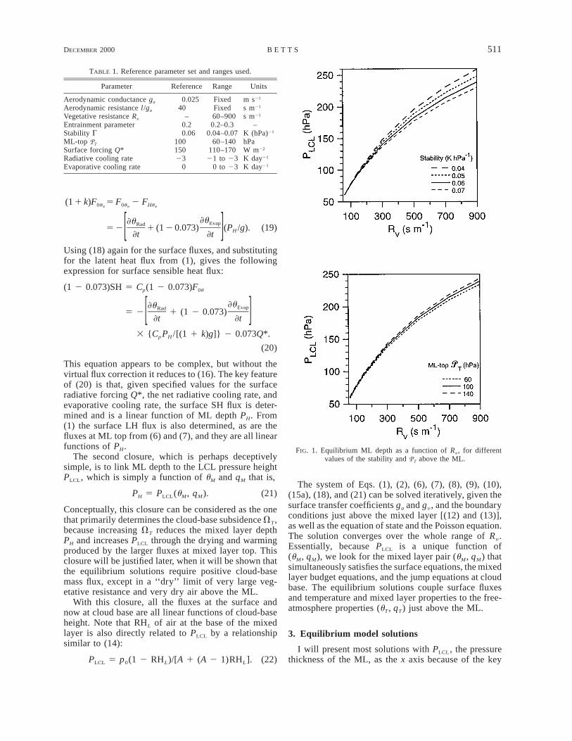
FIG. 1. Equilibrium ML depth as a function of Ry , for differentvalues of the stability and PT above the ML.

(1 1 k)F 5 F 2 F0u 0u Huy y y

]u]u EvapRad5 2 1 (1 2 0.073) (P /g). (19)H[ ]]t ]t

Using (18) again for the surface fluxes, and substitutingfor the latent heat flux from (1), gives the followingexpression for surface sensible heat flux:

(1 2 0.073)SH 5 C (1 2 0.073)Fp 0u

]u]u EvapRad5 2 1 (1 2 0.073)[ ]]t ]t

3 {C P /[(1 1 k)g]} 2 0.073Q*.p H

(20)

This equation appears to be complex, but without thevirtual flux correction it reduces to (16). The key featureof (20) is that, given specified values for the surfaceradiative forcing Q*, the net radiative cooling rate, andevaporative cooling rate, the surface SH flux is deter-mined and is a linear function of ML depth PH. From(1) the surface LH flux is also determined, as are thefluxes at ML top from (6) and (7), and they are all linearfunctions of PH.

The second closure, which is perhaps deceptivelysimple, is to link ML depth to the LCL pressure heightPLCL, which is simply a function of uM and qM that is,

PH 5 PLCL(uM, qM). (21)

Conceptually, this closure can be considered as the onethat primarily determines the cloud-base subsidence VT,because increasing VT reduces the mixed layer depthPH and increases PLCL through the drying and warmingproduced by the larger fluxes at mixed layer top. Thisclosure will be justified later, when it will be shown thatthe equilibrium solutions require positive cloud-basemass flux, except in a ‘‘dry’’ limit of very large veg-etative resistance and very dry air above the ML.

With this closure, all the fluxes at the surface andnow at cloud base are all linear functions of cloud-baseheight. Note that RHL of air at the base of the mixedlayer is also directly related to PLCL by a relationshipsimilar to (14):

PLCL 5 p0(1 2 RHL)/[A 1 (A 2 1)RHL]. (22)

The system of Eqs. (1), (2), (6), (7), (8), (9), (10),(15a), (18), and (21) can be solved iteratively, given thesurface transfer coefficients ga and gy , and the boundaryconditions just above the mixed layer [(12) and (13)],as well as the equation of state and the Poisson equation.The solution converges over the whole range of Ry .Essentially, because PLCL is a unique function of(uM, qM), we look for the mixed layer pair (uM, qM) thatsimultaneously satisfies the surface equations, the mixedlayer budget equations, and the jump equations at cloudbase. The equilibrium solutions couple surface fluxesand temperature and mixed layer properties to the free-atmosphere properties (uT, qT) just above the ML.

3. Equilibrium model solutions

I will present most solutions with PLCL, the pressurethickness of the ML, as the x axis because of the key

512 VOLUME 1J O U R N A L O F H Y D R O M E T E O R O L O G Y

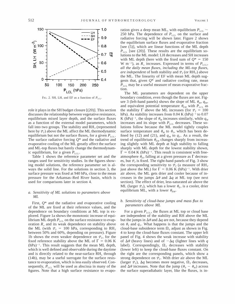
FIG. 2. SH, LH, and EF as a function of PLCL.

role it plays in the SH budget closure [(20)]. This sectiondiscusses the relationship between vegetative resistance,equilibrium mixed layer depth, and the surface fluxesas a function of the external model parameters, whichfall into two groups. The stability and RHT (representedhere by PT) above the ML affect the ML thermodynamicequilibrium but not the surface fluxes, for a given PLCL.The surface radiative forcing Q* and the radiative andevaporative cooling of the ML greatly affect the surfaceand ML-top fluxes but barely change the thermodynam-ic equilibrium, for a given PLCL.

Table 1 shows the reference parameter set and theranges used for sensitivity studies. In the figures show-ing model solutions, the reference parameter set is al-ways the solid line. For the solutions in section 3, thesurface pressure was fixed at 940 hPa, close to the meanpressure for the Arkansas–Red River basin, which isused for comparisons later in section 4.

a. Sensitivity of ML solutions to parameters aboveML

First, Q* and the radiative and evaporative coolingof the ML are fixed at their reference values, and thedependence on boundary conditions at ML top is ex-plored. Figure 1a shows the monotonic increase of equi-librium ML depth PLCL on the surface resistance to evap-oration Ry and its weak dependence on stability abovethe ML (with PT 5 100 hPa, corresponding to RHT

between 50% and 60%, depending on pressure). Figure1b shows the even weaker dependence on PT, for thefixed reference stability above the ML of G 5 0.06 K(hPa)21. This result suggests that the mean ML depth,which is well defined and observable during the daytimeand is directly related to the near-surface RHL through(14b), may be a useful surrogate for the surface resis-tance to evaporation, which is less easily observed. Con-sequently, PLCL will be used as abscissa in many of thefigures. Note that a high surface resistance to evapo-

ration gives a deep mean ML, with equilibrium PLCL ;250 hPa. The dependence of PLCL on the surface andradiative forcing will be shown later. Figure 2 showsthe equilibrium surface fluxes and evaporative fraction[see (5)], which are linear functions of the ML depthPLCL [see (20)]. These results are the equilibrium so-lutions to the ML model: LH decreases and SH increaseswith ML depth (here with the fixed sum of Q* 5 150W m22), as Ry increases. Expressed in terms of PLCL,all the daily mean fluxes, including the ML-top fluxes,are independent of both stability and PT (or RHT) abovethe ML. The linearity of EF with mean ML depth sug-gests that, given Q* and radiative cooling rate, meanPLCL may be a useful measure of mean evaporative frac-tion.

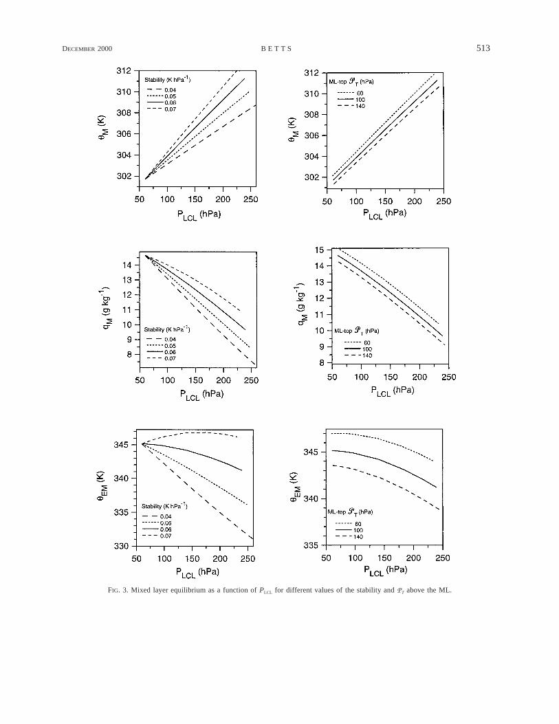
The ML parameters are dependent on the upperboundary condition, even though the fluxes are not. Fig-ure 3 (left-hand panels) shows the slope of ML uM, qM,and equivalent potential temperature uEM with PLCL asthe stability G above the ML increases (for PT 5 100hPa). As stability increases from 0.04 K (hPa)21 to 0.07K (hPa)21, the slope of uM increases similarly, while qM

increases and its slope with PLCL decreases. These so-lutions follow because the ML model tightly couplessurface temperature and uM to uT, which has been de-fined by (12) and (21), and qM to qT. As a result, thetrend of equilibrium uEM changes sharply from increas-ing slightly with ML depth at high stability to fallingsharply with ML depth for the lowest stability shown,G 5 0.04 K (hPa)21. This result is consistent with free-atmosphere uET falling at a given pressure as G decreas-es, but PT is fixed. The right-hand panels of Fig. 3 showthe corresponding sensitivity to PT (a measure of RHT

just above the ML) for G 5 0.06 K (hPa)21. With drierair above, the ML gets drier and cooler because of in-creases in the jumps Du and Dq at ML top (see nextsection). The effect of drier, less-saturated air above theML (larger PT), which has a lower uE, is a cooler, drierequilibrium ML, with a lower uEM.

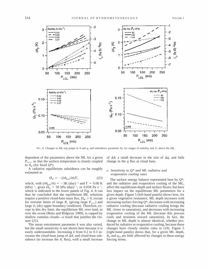
b. Sensitivity of cloud-base jumps and mass flux toparameters above ML

For a given PLCL, the fluxes at ML top or cloud baseare independent of the stability and RH above the MLbut the jumps in Du and Dq are not, because they dependon uT and qT. What happens is that the jumps and thecloud-base subsidence term VT adjust as shown in Fig.4 to keep the cloud-base fluxes constant. The upper leftpanel of Fig. 4 shows the weak increase with stabilityof Du (heavy lines) and of 2Dq (lighter lines with qlabel). Correspondingly, VT decreases with stability(lower left) to keep the cloud-base fluxes constant. Onthe right are the corresponding panels, which show astrong dependence on PT. With drier air above the ML(larger PT), Dq becomes more negative, VT decreases,and Du increases. Note that the jump (u0 2 uM) acrossthe surface superadiabatic layer, like the fluxes, is in-

DECEMBER 2000 513B E T T S

FIG. 3. Mixed layer equilibrium as a function of PLCL for different values of the stability and PT above the ML.

514 VOLUME 1J O U R N A L O F H Y D R O M E T E O R O L O G Y

FIG. 4. Changes in ML-top jumps in u and q, and subsidence parameter VT for ranges of stability and PT above the ML.

dependent of the parameters above the ML for a givenPLCL, so that the surface temperature is closely coupledto uM (for fixed Q*).

A radiative equilibrium subsidence can be roughlyestimated as

VR 5 2(]uRad/]t)/G, (23)

which, with (]uRad/]t) 5 23K (day)21 and G 5 0.06 K(hPa)21, gives VR 5 50 hPa (day)21, or 0.058 Pa s21,which is indicated in the lower panels of Fig. 4. It canthus be concluded that the equilibrium ML solutionsrequire a positive cloud-base mass flux, V* . 0, exceptfor extreme limits of large Ry (giving large PLCL) andlarge PT (dry upper boundary condition). Therefore, ex-cept in this dry limit, the equilibrium ML over land, asover the ocean (Betts and Ridgway 1989), is capped byshallow cumulus clouds—a result that justifies the clo-sure (21).

The mean entrainment parameter k was also varied,but the small sensitivity is not shown here because it iseasily understandable. Increasing k from 0.2 to 0.3 in-creases the cloud-base jump of Duy and cloud-base sub-sidence (to increase the uy flux), with a small increase

of Du, a small decrease in the size of Dq, and littlechange in the q flux at cloud base.

c. Sensitivity to Q* and ML radiative andevaporative cooling rates

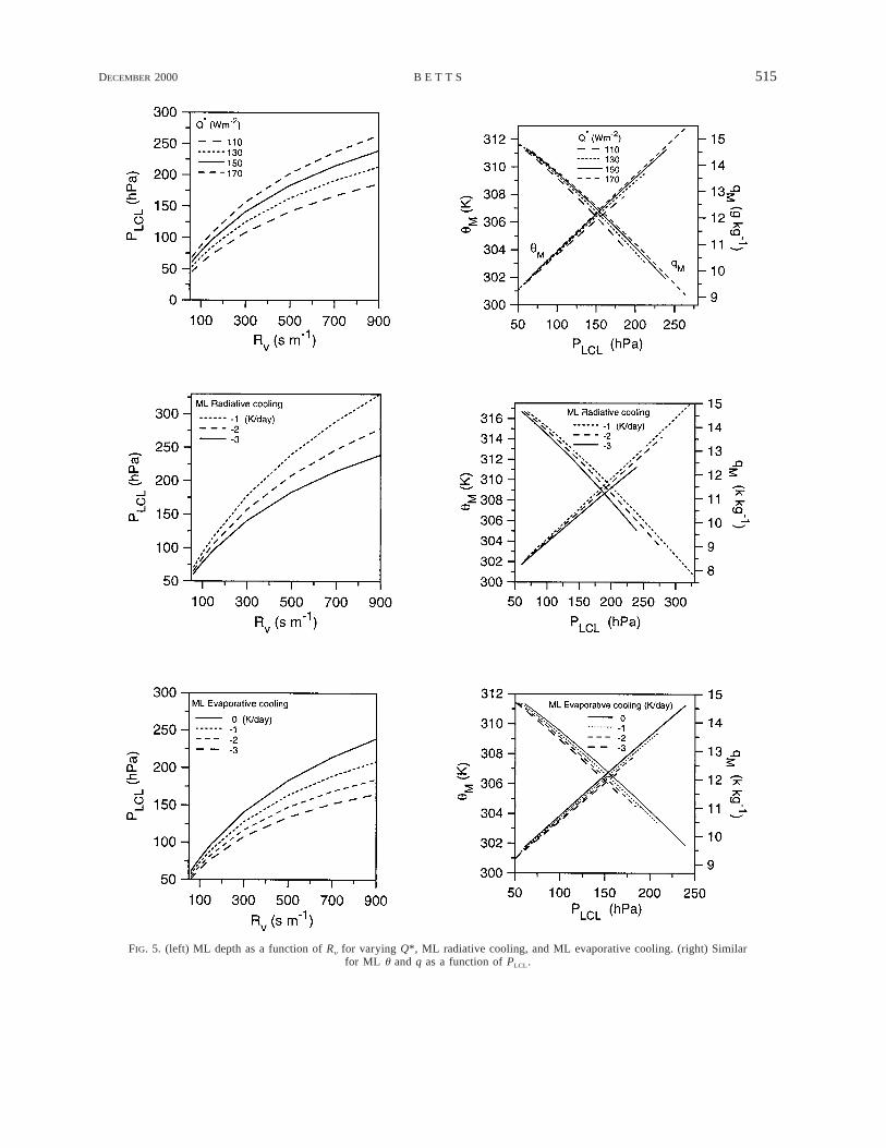
The surface energy balance represented here by Q*,and the radiative and evaporative cooling of the ML,affect the equilibrium depth and surface fluxes, but haveless impact on the equilibrium ML parameters for agiven depth. Figure 5 (left-hand panels) shows how, fora given vegetative resistance, ML depth increases withincreasing surface forcing Q*, decreases with increasingradiative cooling (because radiative cooling brings theML closer to saturation), and decreases with increasingevaporative cooling of the ML (because this processcools and moistens toward saturation). In fact, thechange in ML depth is almost identical, whether pro-duced by radiative or evaporative cooling, because thesechanges have closely similar roles in (19). Figure 5(right-hand panels) shows that, for a given ML depth,uM and qM are little affected by changes in these energyforcing terms.

DECEMBER 2000 515B E T T S

FIG. 5. (left) ML depth as a function of Ry for varying Q*, ML radiative cooling, and ML evaporative cooling. (right) Similarfor ML u and q as a function of PLCL.

516 VOLUME 1J O U R N A L O F H Y D R O M E T E O R O L O G Y

FIG. 6. Variation of (left) SH and (right) LH with ML depth, as a function of Q*, ML radiative, and evaporative cooling (topto bottom).

DECEMBER 2000 517B E T T S

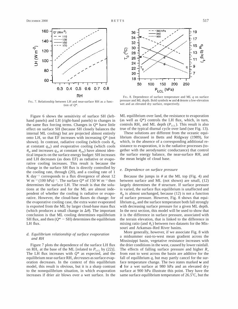
FIG. 7. Relationship between LH and near-surface RH as a func-tion of Q*.

FIG. 8. Dependence of surface temperature and ML q on surfacepressure and ML depth. Bold symbols w and d denote a low-elevationwet and an elevated dry surface, respectively.

Figure 6 shows the sensitivity of surface SH (left-hand panels) and LH (right-hand panels) to changes inthe same flux forcing terms. Changes in Q* have littleeffect on surface SH (because SH closely balances theinternal ML cooling) but are projected almost entirelyonto LH, so that EF increases with increasing Q* (notshown). In contrast, radiative cooling (which cools uM

at constant qM) and evaporative cooling (which coolsuM and increases qM at constant uEM) have almost iden-tical impacts on the surface energy budget: SH increasesand LH decreases (as does EF) as radiative or evapo-rative cooling increases. This result is because thechange in the surface SH flux is directly controlled bythe cooling rate, through (20), and a cooling rate of 1K day21 corresponds to a flux divergence of about 12W m22 (100 hPa)21. The surface Q* of 150 W m22 thendetermines the surface LH. The result is that the solu-tions at the surface and for the ML are almost inde-pendent of whether the cooling is radiative or evapo-rative. However, the cloud-base fluxes do change: forthe evaporative cooling case, the extra water evaporatedis exported from the ML by larger cloud-base mass flux(which produces a small change in Du). The importantconclusion is that ML cooling determines equilibriumSH flux, and then (Q* 2 SH) determines the equilibriumLH flux.

d. Equilibrium relationship of surface evaporationand RH

Figure 7 plots the dependence of the surface LH fluxon RHL at the base of the ML [related to PLCL by (22)].The LH flux increases with Q* as expected, and theequilibrium near-surface RHL decreases as surface evap-oration decreases. In the context of this equilibriummodel, this result is obvious, but it is a sharp contrastto the nonequilibrium situation, in which evaporationincreases if drier air blows over a wet surface. In the

ML equilibrium over land, the resistance to evaporation(as well as Q*) controls the LH flux, which, in turn,controls RHL and ML depth (PLCL). This result is alsotrue of the typical diurnal cycle over land (see Fig. 13).

These solutions are different from the oceanic equi-librium discussed in Betts and Ridgway (1989), forwhich, in the absence of a corresponding additional re-sistance to evaporation, it is the radiative processes (to-gether with the aerodynamic conductance) that controlthe surface energy balance, the near-surface RH, andthe mean height of cloud base.

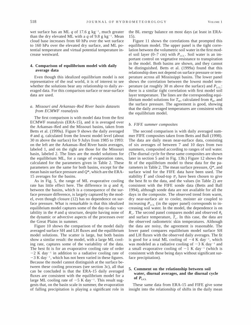
e. Dependence on surface pressure

Because the jumps in u at the ML top (Fig. 4) andbetween surface and ML (not shown) are small, (12)largely determines the u structure. If surface pressureis varied, the surface flux equilibrium is unaffected anduM is almost unchanged, because (12) is not a functionof surface pressure. However, Fig. 8 shows that equi-librium qM and the surface temperature both fall stronglywith decreasing surface pressure for a given ML depth.In the next section, this model will be used to show thatit is the difference in surface pressure, associated withthe terrain elevation, that is linked to the difference inmixing ratio (and uE) between two datasets for the Mis-souri and Arkansas–Red River basins.

More generally, however, if we associate Fig. 8 witha midsummer east-to-west mean gradient across theMississippi basin, vegetative resistance increases withthe drier conditions in the west, caused by lower rainfall.The effects of falling surface pressure and higher Ry

from east to west across the basin are additive for thefall of equilibrium q, but may partly cancel for the sur-face temperature change. The two states marked w andd for a wet surface at 980 hPa and an elevated drysurface at 900 hPa illustrate this point. They have thesame surface equilibrium temperature of 26.58C, but the

518 VOLUME 1J O U R N A L O F H Y D R O M E T E O R O L O G Y

wet surface has an ML q of 17.6 g kg21, much greaterthan the dry elevated ML with a q of 9.8 g kg21. Meancloud base increases from 60 hPa over the wet surfaceto 160 hPa over the elevated dry surface, and ML po-tential temperature and virtual potential temperature in-crease westward.

4. Comparison of equilibrium model with dailyaverage data

Even though this idealized equilibrium model is notrepresentative of the real world, it is of interest to seewhether the solutions bear any relationship to daily av-eraged data. For this comparison surface or near-surfacedata are used.

a. Missouri and Arkansas–Red River basin datasetsfrom ECMWF reanalysis

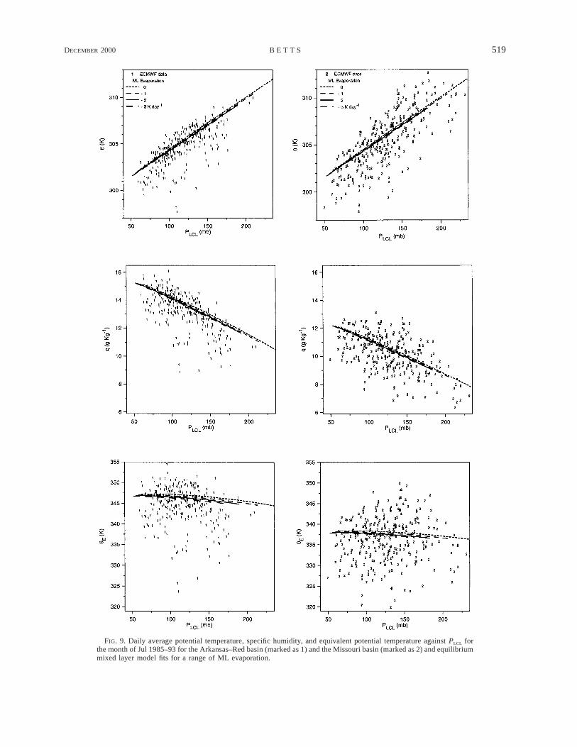
The first comparison is with model data from the firstECMWF reanalysis (ERA-15), and it is averaged overthe Arkansas–Red and the Missouri basins, taken fromBetts et al. (1999a). Figure 9 shows the daily averagedu and q, calculated from the lowest model level (about30 m above the surface) for 9 Julys from 1985 to 1993:on the left are the Arkansas–Red River basin averages,labeled 1, and on the right are those for the Missouribasin, labeled 2. The lines are the model solutions forthe equilibrium ML, for a range of evaporation rates,calculated for the parameters given in Table 2. Theseparameters are the same for both basins, except for themean basin surface pressure and Q*, which are the ERA-15 averages for the basins.

As in Fig. 5, the range of ML evaporative coolingrate has little effect here. The difference in q and uE

between the basins, which is a consequence of the sur-face pressure difference, is largely captured by the mod-el, even though closure (12) has no dependence on sur-face pressure. What is remarkable is that this idealizedequilibrium model captures some of the day-to-day var-iability in the u and q structure, despite having none ofthe dynamic or advective aspects of the processes overthe Great Plains in summer.

Figure 10 shows the comparison of the model dailyaveraged surface SH and LH fluxes and the equilibriummodel solutions. The scatter is large, but both basinsshow a similar result: the model, with a large ML cool-ing rate, captures some of the variability of the data.The best fit is for an evaporative cooling rate of order22 K day21 in addition to a radiative cooling rate of23 K day21, which has not been varied in these figures.Because the model cannot distinguish at the surface be-tween these cooling processes (see section 3c), all thatcan be concluded is that the ERA-15 daily averagedfluxes are consistent with the equilibrium model for alarge ML cooling rate of 25 K day21. This result sug-gests that, on the basin scale in summer, the evaporationof falling precipitation is playing a significant role in

the BL energy balance on most days (at least in ERA-15).

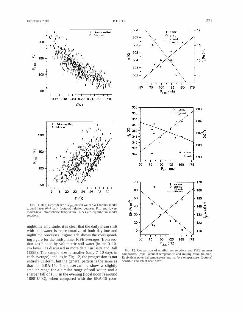
Figure 11 shows the correlations that prompted thisequilibrium model. The upper panel is the tight corre-lation between the volumetric soil water in the first mod-el soil layer (0–7 cm) with PLCL. Soil water is an im-portant control on vegetative resistance to transpirationin the model. Both basins are shown, and they cannotbe distinguished. Betts et al. (1999a) found that thisrelationship does not depend on surface pressure or tem-perature across all Mississippi basins. The lower panelshows the correlation between the lowest model tem-perature (at roughly 30 m above the surface) and PLCL:there is a similar tight correlation with first model soillayer temperature. The lines are the corresponding equi-librium model solutions for TM, calculated from uM, andthe surface pressure. The agreement is good, showingthat the daily averaged temperatures are consistent withthe equilibrium model.

b. FIFE summer composites

The second comparison is with daily averaged sum-mer FIFE composites taken from Betts and Ball (1998).The data are daily mean near-surface data, consistingof six averages of between 7 and 10 days from twosummers, composited according to ranges of soil water.(The diurnal cycle for these same composites are shownlater in section 5 and in Fig. 13b.) Figure 12 shows thefit of the equilibrium model to these data for the pa-rameters in Table 2. The mean surface pressure, Q*, andsurface wind for the FIFE data have been used. Thestability G and cloud-top PT have been chosen to givethe best fit to the data, and the values (in Table 2) areconsistent with the FIFE sonde data (Betts and Ball1994), although sonde data are not available for all thedays in the composite. The observed trend from warm,dry near-surface air to cooler, moister air coupled toincreasing PLCL (in the upper panel) corresponds to in-creasing soil water. In the model, the dependence is onRy . The second panel compares model and observed uE

and surface temperature, To. In this case, the data arethe observed radiometric skin temperatures. Althoughthe data are noisy, the agreement is reasonable. Thelower panel compares equilibrium model surface SHand LH fluxes with the observed daily averages. The fitis good for a total ML cooling of 24 K day21, whichwas modeled as a radiative cooling of 23 K day21 anda small evaporative cooling of 21 K day21 (which isconsistent with these being days without significant sur-face precipitation).

5. Comment on the relationship between soilwater, diurnal averages, and the diurnal cycleof PLCL

These same data from ERA-15 and FIFE give someinsight into the relationship of shifts in the daily mean

DECEMBER 2000 519B E T T S

FIG. 9. Daily average potential temperature, specific humidity, and equivalent potential temperature against PLCL forthe month of Jul 1985–93 for the Arkansas–Red basin (marked as 1) and the Missouri basin (marked as 2) and equilibriummixed layer model fits for a range of ML evaporation.

520 VOLUME 1J O U R N A L O F H Y D R O M E T E O R O L O G Y

TABLE 2. Parameter sets for data comparison.

Parameter Arkansas–Red Missouri FIFE Units

Aerodynamic conductance ga

Aerodynamic resistance, l/ga

Vegetative resistance Ry

Entrainment parameterStability G

0.0254060–900

0.20.06

0.0254060–900

0.20.06

0.04920.460–900

0.20.05

m s21

s m21

s m21

–K (hPa)21

ML-top PT

Surface pressureSurface forcing Q*Radiative cooling rateEvaporative cooling rate

60941158230 to 23

60896141230 to 23

809701672321

hPahPaW m22

K day21

K day21

FIG. 10. Daily average SH and LH against PLCL for the month of Jul 1985–93 for the Arkansas–Red basin (shown by1) and the Missouri basin (shown by 2) and equilibrium mixed layer model fits for a range of BL evaporation.

to shifts in the diurnal pattern. The data have beenbinned by soil water, which is a control on vegetativeresistance in summer in both the ERA model and theFIFE data. Figure 13a shows the mean diurnal cycle ofPLCL, corresponding to the data in Fig. 11a for the Mis-

souri river basin for the month of July 1985–93, binnedby volumetric soil water SW1 in the model 0–7-cm soillayer (using 0.02 intervals). The entire diurnal cycle isshifted upward with decreasing soil water. Although thedaytime amplitude of this shift is a little larger than the

DECEMBER 2000 521B E T T S

FIG. 11. (top) Dependence of PLCL on soil water SW1 for first modelground layer (0–7 cm); (bottom) relation between PLCL and lowestmodel-level atmospheric temperature. Lines are equilibrium modelsolutions.

FIG. 12. Comparison of equilibrium solutions and FIFE summercomposites. (top) Potential temperature and mixing ratio. (middle)Equivalent potential temperature and surface temperature. (bottom)Sensible and latent heat fluxes.

nighttime amplitude, it is clear that the daily mean shiftwith soil water is representative of both daytime andnighttime processes. Figure 13b shows the correspond-ing figure for the midsummer FIFE averages (from sec-tion 4b) binned by volumetric soil water (in the 0–10-cm layer), as discussed in more detail in Betts and Ball(1998). The sample size is smaller (only 7–10 days ineach average), and, as in Fig. 12, the progression is notentirely uniform, but the general pattern is the same asthat for ERA-15. The observations show a slightlysmaller range for a similar range of soil water, and asharper fall of PLCL in the evening (local noon is around1800 UTC), when compared with the ERA-15 com-

522 VOLUME 1J O U R N A L O F H Y D R O M E T E O R O L O G Y

FIG. 13. Mean diurnal cycle, stratified by soil moisture, for (a)Missouri basin for Jul 1985–93 and (b) FIFE 1987 and 1988 mid-summer composites. Local noon (near 1830 UTC) is marked.

posites. Figure 13 shows that soil water decreases,which are linked to increases in vegetative resistance,produce an upward mean shift of saturation pressureheight PLCL, as well as some amplification of the diurnalcycle of PLCL.

6. Conclusions

This equilibrium ML model, although highly simpli-fied, suggests several important conclusions about thecoupling between the surface, the ML, and the atmo-sphere above on timescales longer than the diurnal.First, it shows that the mean ML depth increases asvegetative resistance to evaporation increases. In ad-

dition, the surface radiative forcing also increases MLdepth, but the ML radiative and evaporative coolingprocesses reduce ML depth. Second, the model largelyuncouples mixed layer parameters, as defined by ML uand q, from the ML fluxes. The boundary conditionsabove the ML control u and q but do not affect thefluxes; it is the surface forcing Q* and the radiative andevaporative cooling terms within the ML (together withthe vegetative resistance) that control the mean surfacefluxes and evaporative fraction. Furthermore, for a givenRy , it is the radiative and evaporative cooling terms thatcontrol the surface SH flux; the surface forcing Q* thencontrols the LH flux.

The solutions show that, except for extreme valuesof vegetative resistance and very dry air above the ML,the equilibrium ML is capped by shallow cumulusclouds, as over the ocean. At the same time, as Ry in-creases, the ML structure and depth shift from the oce-anic limit toward a warmer, drier boundary layer. Themodel shows that evaporation controls equilibrium near-surface RH and not vice versa. The equilibrium solu-tions also give insight into how the gradient of meanmixing ratio across the Mississippi basin is linked tochanges in surface pressure as well as vegetative resis-tance to evaporation.

An equilibrium model is over simplified, and the nonlinearities introduced by the diurnal cycle have not beenaddressed, but nonetheless the solutions are a plausiblezero-order fit to daily mean model data for the Missouriand Arkansas–Red River basin averages, shown in Figs.9 and 11, and summer composites from the FIFE ex-periment, shown in Fig. 12. The river basin comparisonssuggest that evaporation of falling precipitation plays asignificant role in determining the mean surface fluxeson this scale. These same data give some insight intothe relationship of shifts in the daily mean to shifts inthe diurnal pattern. Figure 13 shows that decreases insoil water, which are linked to increases in vegetativeresistance, produce an upward mean shift of saturationpressure height PLCL, as well as some amplification ofthe diurnal cycle of PLCL.

The upper boundary closure on potential temperature[12] is an over simplification, although it is also broadlyconsistent with the Missouri and Arkansas–Red Riverbasin averages. A recent radiative convective equilib-rium study of temperature profiles at different heightsby Molnar and Emanuel (1999) suggests that potentialtemperature profiles may be coupled with surface heightabove sea level, not just with pressure height above thesurface, as in (12). In addition, by using the closure,represented by (13), the ML and shallow cumulus layershave been uncoupled, and clearly their coupling de-serves further study. However, this simple model is like-ly to be useful in separating the effect of upper boundaryconditions and internal processes on the mean surfaceequilibrium over land, and in understanding feedbacksat the land surface in coupled models.

DECEMBER 2000 523B E T T S

Acknowledgments. I acknowledge support from theNational Science Foundation under Grant ATM-9988618, from NOAA under Grant NA76-GP0255, andfrom NASA under Grant NAG5-8364. I am grateful tothe reviewers for their helpful comments.

REFERENCES

Beljaars, A. C. M., P. Viterbo, M. J. Miller, and A. K. Betts, 1996:The anomalous rainfall over the United States during July 1993:Sensitivity to land surface parameterization and soil moistureanomalies. Mon. Wea. Rev., 124, 362–383.

Betts, A. K., 1973: Non-precipitating convection and its parameter-ization. Quart. J. Roy. Meteor. Soc., 99, 178–196., 1975: Parametric interpretation of trade-wind cumulus budgetstudies. J. Atmos. Sci., 32, 1934–1945., 1997: The parameterization of deep convection. The Physicsand Parameterization of Moist Atmospheric Convection, R. K.Smith, Ed., NATO ASI Series C, Vol. 505, Kluwer Academic,255–279., and W. Ridgway, 1988: Coupling of the radiative, convective,and surface fluxes over the equatorial Pacific. J. Atmos. Sci., 45,522–536., and , 1989: Climatic equilibrium of the atmospheric con-vective boundary layer over a tropical ocean. J. Atmos. Sci., 46,2621–2641., and , 1992: Tropical boundary layer equilibrium in the lastice age. J. Geophys. Res., 97, 2529–2534., and J. H. Ball, 1994: Budget analysis of FIFE 1987 sonde data.J. Geophys. Res., 99, 3655–3666., and , 1995: The FIFE surface diurnal cycle climate. J.Geophys. Res., 100, 25 679–25 693., and , 1998: FIFE surface climate and site-average dataset:1987–1989. J. Atmos. Sci., 55, 1091–1108., , A. C. M. Beljaars, M. J. Miller, and P. Viterbo, 1996:The land-surface–atmosphere interaction: A review based on ob-servational and global modeling perspectives. J. Geophys. Res.,101, 7209–7225.

, P. Viterbo, and E. Wood, 1998: Surface energy and water bal-ance for the Arkansas–Red River basin from the ECMWF re-analysis. J. Climate, 11, 2881–2897., J. H. Ball, and P. Viterbo, 1999a: Basin-scale surface waterand energy budgets for the Mississippi from the ECMWF re-analysis. J. Geophys. Res., 104, 19 293–19 306., M. L. Goulden, and S. C. Wofsy, 1999b: Controls on evapo-ration in a boreal spruce forest. J. Climate, 12, 1601–1618.

Carson, D. J., 1973: The development of a dry inversion-cappedconvectively unstable boundary layer. Quart. J. Roy. Meteor.Soc., 99, 450–467.

Clement, A., and R. Seager, 1999: Climate and the tropical oceans.J. Climate, 12, 3383–3401.

De Ridder, K., 1997: Land surface processes and the potential forconvective precipitation. J. Geophys. Res., 102, 30 085–30 090., 1998: The impact of vegetation cover on Sahelian droughtpersistence. Bound.-Layer Meteor., 88, 307–321.

Eltahir, E. A. B., 1998: A soil moisture rainfall feedback mechanism.1: Theory and observations. Water Resour. Res., 34, 765–776.

Kim, J., and S. B. Verma, 1990: Components of the surface energybalance in a temperate grassland ecosystem. Bound.-Layer Me-teor., 51, 401–417.

Lilly, D. K., 1968: Models of cloud-topped mixed layers under astrong inversion. Quart. J. Roy. Meteor. Soc., 94, 292–309.

Molnar, P., and K. A. Emanuel, 1999: Temperature profiles in radi-ative–convective equilibrium above surfaces at different heights.J. Geophys. Res., 104, 24 265–24 271.

Monteith, J. L., 1981: Evaporation and surface temperature. Quart.J. Roy. Meteor. Soc., 107, 1–21.

Pierrehumbert, R. T., 1995: Thermostats, radiator fins, and the run-away greenhouse. J. Atmos. Sci., 52, 1784–1806.

Sarachik, E. S., 1978: Tropical sea surface temperature: An interactiveone-dimensional atmosphere–ocean model. Dyn. Atmos. Oceans,2, 450–469.

Schar, C., D. Luthi, U. Beyerle, and E. Heise, 1999: The soil–pre-cipitation feedback: A process study with a regional climatemodel. J. Climate, 12, 722–741.

Tennekes, H. A., 1973: Model for the dynamics of the inversion abovea convective boundary layer. J. Atmos. Sci., 30, 558–567.