
I Vol. 11 No. 2 - AMH International
149
Journal of Economics and Behavioral Studies (JEBS) Vol. 11, No. 2, April 2019 (ISSN 2220-6140) I Published by AMH International Vol. 11 No. 2 ISSN 2220-6140
-
Upload
khangminh22 -
Category
Documents
-
view
3 -
download
0
Transcript of I Vol. 11 No. 2 - AMH International

Journal of Economics and Behavioral Studies (JEBS) Vol. 11, No. 2, April 2019 (ISSN 2220-6140)
I
Published by
AMH International
Vol. 11 No. 2 ISSN 2220-6140

Journal of Economics and Behavioral Studies (JEBS) Vol. 11, No. 2, April 2019 (ISSN 2220-6140)
II
Editorial Journal of Economics and Behavioral Studies (JEBS) provides distinct avenue for quality research in the ever-changing fields of economics & behavioral studies and related disciplines. Research work submitted for publication consideration should not merely limited to conceptualization of economics and behavioral developments but comprise interdisciplinary and multi-facet approaches to economics and behavioral theories and practices as well as general transformations in the fields. Scope of the JEBS includes: subjects of managerial economics, financial economics, development economics, finance, economics, financial psychology, strategic management, organizational behavior, human behavior, marketing, human resource management and behavioral finance. Author(s) should declare that work submitted to the journal is original, not under consideration for publication by another journal, and that all listed authors approve its submission to JEBS. Author (s) can submit: Research Paper, Conceptual Paper, Case Studies and Book Review. Journal received research submission related to all aspects of major themes and tracks. All submitted papers were first assessed by the editorial team for relevance and originality of the work and blindly peer-reviewed by the external reviewers depending on the subject matter of the paper. After the rigorous peer-review process, the submitted papers were selected based on originality, significance, and clarity of the purpose. The current issue of JEBS comprises of papers of scholars from South Africa, Nigeria, Namibia and Zambia. Export function of cocoa production, exchange rate volatility and prices, nexus between consumer confidence and economic growth, causal relationship between private sector credit extended and economic growth, significant factors influencing quality assurance practices, assessment of the employee job satisfaction, trade in services-economic growth nexus, customer interactions through customer-centric technology, mobile technology as a learning tool in the academic environment, effects of public expenditure on gross domestic product, revenue productivity of the tax system, banking sector development transmission mechanism of financial development and dynamics of ethnic politics in nigeria were some of the major practices and concepts examined in these studies. Current issue will therefore be a unique offer where scholars will be able to appreciate the latest results in their field of expertise, and to acquire additional knowledge in other relevant fields. Prof. Sisira R N Colombage, Ph. D. Editor In Chief

Journal of Economics and Behavioral Studies (JEBS) Vol. 11, No. 2, April 2019 (ISSN 2220-6140)
III
Editorial Board
Saqib Muneer PhD, Hail University, KSA
Prof Mehmed Muric PhD, Global Network for Socioeconomic Research & Development, Serbia
Rajarshi Mitra PhD, National Research University, Russian Federation
Ravinder Rena PhD, Monarch University, Switzerland
Alexandru Trifu PhD, University, Petre Andrei, Iasi Romania
Apostu Iulian PhD, University of Bucharest, Romania
Sisira R N Colombage PhD, Monash University, Australia
Chux Gervase Iwu PhD, Cape Peninsula University of Technology, South Africa
Hai-Chin YU PhD, Chung Yuan University,Chungli, Taiwan
Anton Miglo PhD, School of business, University of Bridgeport, USA
Elena Garcia Ruiz PhD, Universidad de Cantabria, Spain
Fuhmei Wang PhD, National Cheng Kung University, Taiwan
Khorshed Chowdhury PhD, University of Wollongong, Australia
Pratibha Samson Gaikwad PhD, Shivaji University of Pune, India
Mamta B Chowdhury PhD, University of Western Sydney, Australia

Journal of Economics and Behavioral Studies (JEBS) Vol. 11, No. 2, April 2019 (ISSN 2220-6140)
IV
Table of Contents
Description Pages Title I Editorial II Editorial Board III Table of Contents IV Papers V Export Function of Cocoa Production, Exchange Rate Volatility and Prices in Nigeria Alaba David Alori, Adebayo Augustine Kutu
1
The Nexus between Consumer Confidence and Economic Growth in South Africa: An ARDL Bounds Testing Approach Khayelihle Madlopha
15
Examining the Causal Relationship between Private Sector Credit Extended and Economic Growth in Namibia Andreas, J P S Sheefeni
23
Significant Factors Influencing Quality Assurance Practices in Small and Medium-Sized Construction Projects in South Africa Kgashane Stephen Nyakala, Thinandavha Thomas Munyai, Jan-Harm Pretorius, Andre Vermeulen
30
An Assessment of the Employee Job Satisfaction: Views from Empirical Perspectives Albert Tchey Agbenyegah
45
Trade in Services-Economic Growth Nexus: An Analysis of the Growth Impact of Trade in Services in SADC Countries Alexander Maune
58
Enhanced Customer Interactions through Customer-Centric Technology within a Call Centre Devina Oodith
79
Mobile Technology as a Learning Tool in the Academic Environment Sidwell Sabelo Nkosi, Rosemary Sibanda, Ankit Katrodia
92
Effects of Public Expenditure on Gross Domestic Product in Zambia from 1980-2017: An ARDL Methodology Approach Mubanga Mpundu, Jane Mwafulirwa, Mutinta Chaampita, Notulu Salwindi
103
Revenue Productivity of the Tax System in Namibia: Tax Buoyancy Estimation Approach J P S Sheefeni, A Shikongo, O Kakujaha-Matundu, T Kaulihowa
112
Investigating the Banking Sector Development Transmission Mechanism of Financial Development to Growth: Evidence from Sub-Saharan Africa (SSA) Tochukwu Timothy Okoli, Ajibola Rhoda Oluwafisayomi
120
Dynamics of Ethnic Politics in Nigeria: An Impediment to its Political System Toyin Cotties Adetiba
132

Journal of Economics and Behavioral Studies (JEBS) Vol. 11, No. 2, April 2019 (ISSN 2220-6140)
V
PAPERS
Journal of Economics and Behavioral Studies (JEBS) Vol. 11, No. 2, April 2019 (ISSN 2220-6140)
1
Export Function of Cocoa Production, Exchange Rate Volatility and Prices in Nigeria
Alaba David Alori1 Adebayo Augustine Kutu2 1Department of Agricultural Economics & Extension, Federal University of Technology, Minna, Nigeria
2School of Accounting, Economics & Finance, University of KwaZulu-Natal, South Africa [email protected]
Abstract: This study examined the export function of cocoa production and determined the impact of exchange rates and price volatility on the exportation of cocoa in Nigeria. The Phillips-Perron (PP) and Augmented Dickey-Fuller (ADF) unit root tests, Ordinary Least Square (OLS) and Structural Vector Autoregressive (SVAR) methodologies were employed to analyse the time series data that spanning from 1970:01 to 2016:12. The PP and ADF unit root tests findings indicated that none of the variables was stationary at levels (I (0)) however, after the first difference I (1) they became stationary. At 5%, the OLS results showed that all the variables were statistically significant in analysing the effects of exchange rates and price volatility on the value of cocoa production in Nigeria. The price of cocoa in the international market and the value of exchange rates play a significant role in cocoa exports growth in Nigeria. Further, findings from the SVAR showed that an increase in the price of cocoa would increase cocoa production and cocoa export growth in Nigeria, while the exchange rate volatility would affect cocoa export growth in Nigeria. The result further revealed that the shocks to exchange rate accounted for the greater volatility (positively significant for the entire period) to the value of cocoa exported, as against other variables in the model. Based on those findings, the paper, therefore, recommends that there should be a free exchange rate market determination, in order to enhance the export growth and increase cocoa output in Nigeria. Keywords: Cocoa production, exchange rate volatility and prices.
1. Introduction The cocoa sub-sector of the Nigerian economy has received increasing attention as an essential part of the current economic reform agenda of the federal government on diversification of the nation’s export base from crude oil and boost agricultural production. The performances of the agricultural export fell below equality and the agricultural sector experienced a persistent decline after economic reform undertaken through the Structural Adjustment program (SAP) of 1986 whereas this sector was a major contributor to Nigeria’s foreign exchange earnings. Prior to the 1980s, cocoa was a major source of foreign exchange earnings, the leading agricultural export commodity and economic development in Nigeria (Abang & Ndifon, 2002; Nkang et al., 2006). Through the devaluation of the Nigerian naira in 1986, the demand for agricultural products was increased while its price was raised over the years (Adubi & Okunmadewa, 1999). There was instability of the exchange rate movement due to the devaluation policy and this raised concerns about the effect of such policy on the flow of agricultural trade in the Nigerian economy (Okunmadewa, 1999). Both the exchange rates and prices of cocoa export in Nigeria between 1970 and 1977 were stable. This stability was attributed to the Nigeria Commodity Board (NCB) policy impacting on the controlled export prices. However, there was an exchange rates upsurge, between 1978 and 1982, exasperated by the introduction of both dollars pegged systems and managed float of exchange rate policies in the Nigerian economy. Hence, this fluctuation declined the quantity of exportation of cocoa. In view of the instability of exchange rate, price volatilities and the declining trend of the quantity of cocoa export, this study examines the export function of cocoa production and determines the impact of price and exchange rate volatility on cocoa export growth in Nigeria. Although the impacts of volatilities of exchange rate on international agricultural trade have been investigated by some scholars (Weersink et al., 2008; IFPRI, 2011; Braun & Tadesse, 2012), however, the impacts of price volatility have not been largely investigated in the extant literature, hence, this paper tends to contribute to the body of knowledge. Following this introduction other sections of this paper is structured as follows: Section 2 is the justification of the study; Section 3 is a brief review of the empirical research; Section 4 outlines the methodology employed; Section 5 presents the empirical results and data analysis, while Section 6 concludes the paper by explaining the summary of the findings with empirical comparisons from Nigeria.
Journal of Economics and Behavioral Studies (JEBS) Vol. 11, No. 2, April 2019 (ISSN 2220-6140)
2
Justification of the Study: Since the collapse of the Bretton Woods system of the 1970s, researchers became interested in the impacts of exchange rate volatility on exports due to the fact that among major currencies in the world, fixed exchange rates system was allowed to float. Changes in income earnings of export crop producers come as a result of either the devaluation of the currency, a decrease or increase in the international price of exports, and the subsequent increase in producer prices. Such exchange rate/price changes if they are erratic could, however, result in a large reduction in future output. Fluctuations, either positive or negative, are not desirable as they increase uncertainty and risk in international transactions and bye and bye, trade is discouraged. A study conducted by the IMF (1984) indicated that volatility in the exchange rate when compared to currency in term of foreign ones is a random movement of domestic prices. Price instability and Exchange rate volatility result in uncertainties and risks in the international market and thereby discouraging trade. The risk involved in exchange rate measures the erratic pattern and volatility of movement in the exchange rate. The more volatile the movement, the greater the uncertainty and risks involved and this eventually leads to price instability. The prices the producers receive appear to be main concern of the producers; hence, they are mostly interested in the price stability of such products, as it relates to earning a consistent income. Therefore, one of the factors that have been identified as a determinant of price instability is exchange rate volatility, and this is impacting on cocoa production and export of cocoa in Nigeria. Hence, the need to be empirically resolved and studies this concept more closely. 2. Empirical Review on Price and Exchange Rate Volatility and Agricultural Trade Despite the numerous extant literature on the impact of exchange rate volatility on trade, it appears that no existing study has simultaneously explored the contribution of price volatilities and exchange rate on agricultural trade (though such studies have been conducted separately) in Nigeria. Agricultural trade has been found to be more sensitive to uncertainties of exchange rate in the developing countries when compared to other sectors. Adopting a sample of the flow of bilateral trade across G10 nations, when compared to other sectors, Chou et al. (2000) indicate that the real exchange rate uncertainty has had a significant negative effect on agricultural trade. Again, Kandilov (2008) argues that when compared to exporters in the developed countries, the impact of exchange rate volatilities is higher for developing country exporters. Hence, he concludes that agricultural exports among the developing economies are more susceptible to exchange rate volatilities, as compared to developed countries. In addition, Villanueva and Sarker (2009) conducted a study to investigate the impacts of exchange rate volatility on the importation of fresh tomato into the United States from Mexico. Adopting the cointegration analysis, the study indicated that while changes in exchange rate have a positive impact on trade flows; volatility of the exchange rate has a significant negative contribution to the flow of trade. A similar study was again conducted in Cameroon, on the behavior of agricultural export by Tshibaka (1997). He estimated the impacts of exchange rate policies on crop prices on Cameroon’s agricultural export competitiveness. The outcome of the study indicates that exchange rate volatility has a significant negative impact on the flow of trade. Several other researchers such as Johnson et al. (1977), Schwartz (1986), Bradshaw and Ordan (1990), Denbaly and Torgerson (1992), Babula et al. (1995), Kiptui (2007), Aliyu (2008) and Oyinlola (2008), all investigated the impact of exchange rate volatility on agricultural trade and showed that exchange rate volatility has a significant effect on the export of agricultural product. The volatile market prices has indicated that price volatility is probably one of the main sources of risk and an important feature of agricultural markets in international agricultural trade. Changes in prices have been shown to have remarkable implications on the allocation of resources, as well as producer and consumer welfare. To this end price volatility may have a negative effect at the microeconomic level of poverty and growth in the developing economies (Aizenman & Marion, 1993; Ramey & Ramey, 1995). Some economists suggest that there is a level of connection between crises and price volatility; firstly, higher price volatility could be leading to an economic crisis (Aizenman & Pinto, 2005; Acemoglu et al., 2003). Secondly, commodity price volatility may also contribute to governments and farmers household decisions. As argued by Dehn et al. (2005), price risk is one of the most important components of risk faced by households and not solely on earnings. Gilbert (2006) further conducted a study where he showed that agricultural price volatility was higher in the 1970s than in the 1960s, although there was a remarkable decline in the second half of 1980s and the 1990s respectively. It has however maintained a steady growth

Journal of Economics and Behavioral Studies (JEBS) Vol. 11, No. 2, April 2019 (ISSN 2220-6140)
3
above the level of the 1960s and persisted till date. Overall, it is in view of this high volatility in prices that this study deemed it important to simultaneously examine the export function of cocoa production and determines the effect of price and exchange rate volatility on cocoa export growth in Nigeria. This study may help policymakers in the design of appropriate policies and to help market participants to better accommodate these phenomena (price and exchange rate volatility). 3. Research Methodology In achieving the study’s objective, the following information criteria are important for the estimating techniques that were adopted for the study. In addition, this study may suggest policies that can help to mitigate the risk of price volatility. Scope of the Study, Data and Data Sources: Monthly data from 1970 to 2016 were employed for this study. Data on real Gross Domestic Product (GDP), cocoa output (OUTPUT), the value of cocoa (QXP), exchange rate (EXR), price indexes of cocoa (COCOAP) and consumer price index (CPI) were employed for the econometrics analyses. The data were sourced from the Central Bank of Nigeria's Statistical Bulletin, Annual Report and Statement of Accounts and the Trade Summary published by the National Bureau of Statistics (NBS) and World Bank. Application of the Export Supply Model for Cocoa: In order to examine the export function of cocoa production in Nigeria, this study follows the view of Mehare and Edriss (2012), where the export supply model for cocoa are presented using the Ordinary Least Square (OLS) method as: ………………..……(4.1.1) Where is the intercept 1 to 2 are coefficients. represents the value of cocoa output exported at time t which is captured by QXP. is the error term. Tests for Unit Root for the OLS Methodology: Several methods can be used to test the stationarity of the data set. However, the common ones are: Augmented Dickey-Fuller (ADF) test and Phillips-Perron (PP) test. In this study, both tests were employed in order to allow for robustness check. The unit root test equation can be presented as: …………….…… (4.2.1) Where the deterministic trend is deducted from . In practice, and are unknown and have to be estimated. The model can be rewritten as: …………………..………………………. (4.2.2) Which includes an intercept and a trend that, is …………………………………………………….…………. (4.2.3) Where and If, the Autoregressive (AR) process has no unit root. Structural Vector Autoregressive (SVAR) Methodology: In line with the SVAR of Stock and Waston (2005), this study determines the effects of price and exchange rate volatility of cocoa using an SVAR in level. The level SVAR is employed owing to its good economic interpretation that can be derived from its impulse response functions. For example, the Vector Error Correction Model (VECM)’s impulse response assumes that the impact of volatilities is permanent; the level SVAR’s impulse response functions allow time and history to determine whether the impact of volatilities is permanent or not (Ramswamy & Sloek, 1998). In addition, the level SVAR is easy to compute and interpret. These merits, therefore, make it attractive to this study to use the SVAR methodology in this study. Assuming the Nigerian economy can be given according to the following equation: …………………………………………………………(4.3.1)

Journal of Economics and Behavioral Studies (JEBS) Vol. 11, No. 2, April 2019 (ISSN 2220-6140)
4
Where is a (k by k) matrix that is explaining the immediate relationship amongst the variables employed is a (k by 1) vector of endogenous variables in which ( = , ,……. ); Co is a (k by 1) vector of
constants; ….. are (k by k) matrix of coefficients of endogenous variables; Z is a (k by k) matrix in which
the elements allow for an immediate effect of certain shocks on the endogenous variable; and t is an error term. Equation 4.3.1 can’t be estimated straight way due to the immediate reaction innate in the SVAR system (Enders, 2004). The SVAR integrates feedback since the endogenous variables affect each other, both in the present and the past time of . Hence, the parameters are unidentified and it is impossible to determine their values (McCoy, 1997). Nevertheless, the figures can be determined by estimating a reduced form SVAR inherent in the equation (Ngalawa & Viegi, 2001). To do this, we pre-multiplied equation 4.3.1 by an inverse of as below:
…………………...(4.3.2)
This provides:
)
However, if we further denote
Therefore, equation (4.3.1) becomes: … (4.3.4)
The change between equations (4.3.1) and (4.3.4) is that “the first is a long-form SVAR where all variables have an immediate effect on each other, while the second is a reduced form SVAR, where no variable has an immediate effect on each other in the model” Enders (2004). More so, is a composite of the volatility in as further revealed by Enders (2004). Matrix Formation and the Imposition of Restrictions on the SVAR Methodology: Following the view of Buckle et al. (2007), the SVAR approach involves the imposition of restrictions on the parameters to derive a sound economic structure. The restrictions limit the responsiveness to variations that creates volatilities in the system that satisfies the expected sign in the reactions of main variables in the model (see Dungey & Fry, 2007; 2009). The primitive restriction ranges from to that capture immediate responses in the system, while the “0” captures the sluggish response in the SVAR relationships. Based on equation 4.3.5, a total of seventeen (17) zero restrictions were imposed on matrix A on the left hand side which allows matrix covariance to be restricted and the diagonal is controlled to be “1”. On the other hand, the matrix B in the right-hand is the diagonal matrix that is uncorrelated. In total, six by six matrices were modeled for this study, using the short run structural restrictions AB-model of Amisano and Gianini (1997), as presented in equation 4.3.5.
=
……….. (4.3.5)
The matrix above in equation 3.3.5 is a 6 by 6 matrixes capturing the 6-variables used in the model
where the
are the vectors in the reduced
form and
are the structural shocks linked to the corresponding equations that captures volatility in the model. Conversely, the way variables affect each other depends on their location in the matrix. The variables are ordered following economic principle of Pesaran and Shin (1998) to prevent arbitrary ordering. For example, row 1 measures the effect of real GDP on the economy. It shows that GDP only responds instantaneously to its own value, while equations 2 and 3 indicate the value of cocoa and cocoa output. The value of cocoa (QXP) responds to GDP and its own lagged value, while and indicates that the cocoa output reacts instantaneously to . Equation 4 is the exchange rate (EXR) which only shows the immediate reaction of cocoa price, as shown by while equations 5 and 6 define the international and domestic goods market price. The COCOAP responds instantaneously to OUTPUT and prices (CPI), while CPI responds instantaneously to all the variables (GDP, QXP, OUTPUT, EXR and COCOAP).

Journal of Economics and Behavioral Studies (JEBS) Vol. 11, No. 2, April 2019 (ISSN 2220-6140)
5
The Lag Selection: The lag selection also refers to the lag length determination that deals with the time between exchange rate volatility, prices and the export growth of cocoa in Nigeria. The monthly data are being employed in this study, in order to have a better estimate with a large degree of freedom. Since the data are monthly, the choice of lag selections is drawn from an optimum lags order using the Akaike Information Criterion (AIC), Schwarz Information Criterion (SIC) and Hannan-Quinn Criterion (HQC). These three types of lag orders are the most commonly used in literature, to select the minimum likely lag length. The basic formula for determining the lag length according to Green (2002) is given as:
…………………………………………………………..………. (4.4.1)
4. Empirical Results and Data Analysis This part contains the interpretation of the results obtained from the methodologies employed. The and methodologies were employed to determine the impact of volatilities on the export function of cocoa production in Nigeria. The results obtained from these procedures are given below: Unit Root Testing Result: For the OLS methodology, this study tested for unit root using the dynamic version of ADF and PP-Fisher at constant and constant plus trend in order to prevent spurious results. Table 1: ADF Unit Root Tests Variables ADF-Fisher Unit root-test (Constant) ADF Unit root-test (Constant, Linear Trend)
Order of integration
t* Statistics P Value Order of integration
t* Statistics P- Value
GDP I(1) -2.868768 0.0498*** I(1) -4.188378 0.0050*** QXP I(1) -3.607183 0.0060*** I(1) -4.320073 0.0031***
OUTPUT I(1) -5.520343 0.0000*** I(1) -5.651736 0.0000***
EXR I(1) -4.725457 0.0001*** I(1) -4.932052 0.0003***
COCOAP I(1) -4.163242 0.0008*** I(1) -5.213600 0.0001***
CPI I(1) -6.881738 0.0000*** I(1) -6.877595 0.0000*** “***” “**” and “*” represent statistical significance at 1%, 5%, and 10% respectively. Table 2: PP- Fisher Chi-Square Unit Root Tests Variables PP Unit-root test (Constant) PP Unit-root test (Constant, Linear Trend)
Order of integration
t* Statistics P Value Order of integration
t* Statistics P- Value
GDP I(1) -14.84498 0.0000*** I(1) -16.30299 0.0000***
QXP I(1) -16.72694 0.0000*** I(1) -17.23177 0.0000*** OUTPUT I(1) -17.94294 0.0000*** I(1) -17.99560 0.0000*** EXR I(1) -17.63672 0.0000*** I(1) -17.69894 0.0000*** COCOAP I(1) -17.00294 0.0000*** I(1) -17.11847 0.0000*** CPI I(1) -17.18908 0.0000*** I(1) -17.18393 0.0000***
“***” “**” and “*” represent statistical significance at 1%, 5%, and 10% respectively. Table 3: Descriptive Analysis DQXP DGDP DOUTPUT DEXR DCOCOAP DCPI Mean 339016.0 557.0801 0.058477 0.313878 910.9238 0.011055 Median 1236.861 440.9583 0.388889 0.005278 3.625000 0.054924 Maximum 21576317 7858.840 70.84375 27.64293 79205.80 17.65566 Minimum -9281561. -7070.157 -78.72106 -11.66076 -38721.41 -18.12400 Std. Dev. 1422016. 1092.513 8.052284 1.742236 5641.838 2.153193 Skewness 6.778065 -0.408666 -0.736893 7.500738 6.014034 -0.293789 Kurtosis 106.1510 14.66651 56.61547 132.5890 90.35573 34.25214
Journal of Economics and Behavioral Studies (JEBS) Vol. 11, No. 2, April 2019 (ISSN 2220-6140)
6
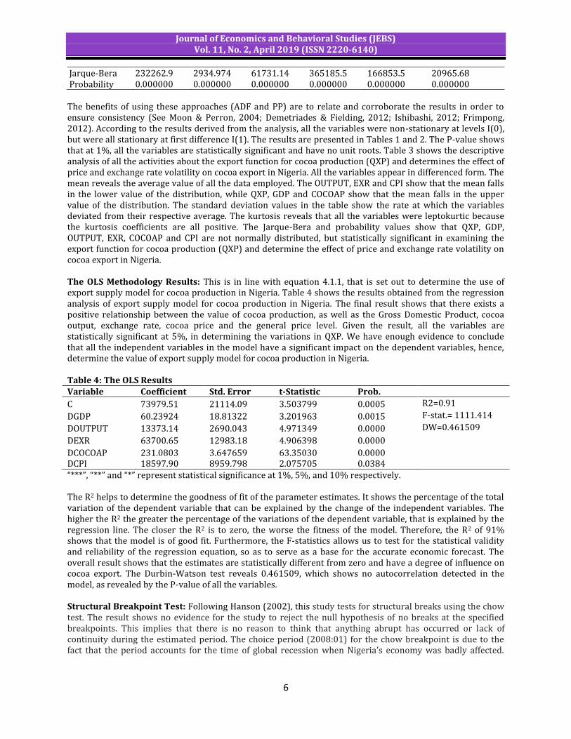
Jarque-Bera 232262.9 2934.974 61731.14 365185.5 166853.5 20965.68 Probability 0.000000 0.000000 0.000000 0.000000 0.000000 0.000000 The benefits of using these approaches (ADF and PP) are to relate and corroborate the results in order to ensure consistency (See Moon & Perron, 2004; Demetriades & Fielding, 2012; Ishibashi, 2012; Frimpong, 2012). According to the results derived from the analysis, all the variables were non-stationary at levels I(0), but were all stationary at first difference I(1). The results are presented in Tables 1 and 2. The P-value shows that at 1%, all the variables are statistically significant and have no unit roots. Table 3 shows the descriptive analysis of all the activities about the export function for cocoa production (QXP) and determines the effect of price and exchange rate volatility on cocoa export in Nigeria. All the variables appear in differenced form. The mean reveals the average value of all the data employed. The OUTPUT, EXR and CPI show that the mean falls in the lower value of the distribution, while QXP, GDP and COCOAP show that the mean falls in the upper value of the distribution. The standard deviation values in the table show the rate at which the variables deviated from their respective average. The kurtosis reveals that all the variables were leptokurtic because the kurtosis coefficients are all positive. The Jarque-Bera and probability values show that QXP, GDP, OUTPUT, EXR, COCOAP and CPI are not normally distributed, but statistically significant in examining the export function for cocoa production (QXP) and determine the effect of price and exchange rate volatility on cocoa export in Nigeria. The OLS Methodology Results: This is in line with equation 4.1.1, that is set out to determine the use of export supply model for cocoa production in Nigeria. Table 4 shows the results obtained from the regression analysis of export supply model for cocoa production in Nigeria. The final result shows that there exists a positive relationship between the value of cocoa production, as well as the Gross Domestic Product, cocoa output, exchange rate, cocoa price and the general price level. Given the result, all the variables are statistically significant at 5%, in determining the variations in QXP. We have enough evidence to conclude that all the independent variables in the model have a significant impact on the dependent variables, hence, determine the value of export supply model for cocoa production in Nigeria. Table 4: The OLS Results Variable Coefficient Std. Error t-Statistic Prob.
C 73979.51 21114.09 3.503799 0.0005 R2=0.91
DGDP 60.23924 18.81322 3.201963 0.0015 F-stat.= 1111.414
DOUTPUT 13373.14 2690.043 4.971349 0.0000 DW=0.461509
DEXR 63700.65 12983.18 4.906398 0.0000
DCOCOAP 231.0803 3.647659 63.35030 0.0000
DCPI 18597.90 8959.798 2.075705 0.0384 “***”, “**” and “*” represent statistical significance at 1%, 5%, and 10% respectively. The R2 helps to determine the goodness of fit of the parameter estimates. It shows the percentage of the total variation of the dependent variable that can be explained by the change of the independent variables. The higher the R2 the greater the percentage of the variations of the dependent variable, that is explained by the regression line. The closer the R2 is to zero, the worse the fitness of the model. Therefore, the R2 of 91% shows that the model is of good fit. Furthermore, the F-statistics allows us to test for the statistical validity and reliability of the regression equation, so as to serve as a base for the accurate economic forecast. The overall result shows that the estimates are statistically different from zero and have a degree of influence on cocoa export. The Durbin-Watson test reveals 0.461509, which shows no autocorrelation detected in the model, as revealed by the P-value of all the variables. Structural Breakpoint Test: Following Hanson (2002), this study tests for structural breaks using the chow test. The result shows no evidence for the study to reject the null hypothesis of no breaks at the specified breakpoints. This implies that there is no reason to think that anything abrupt has occurred or lack of continuity during the estimated period. The choice period (2008:01) for the chow breakpoint is due to the fact that the period accounts for the time of global recession when Nigeria’s economy was badly affected.

Journal of Economics and Behavioral Studies (JEBS) Vol. 11, No. 2, April 2019 (ISSN 2220-6140)
7
However, the National Bureau of Statistics (NBS) revealed that Nigeria exited recession in the third and fourth quarters of 2008. Table 5: Structural Breakpoint Test Chow Breakpoint Test: 2008M01 F-statistic 1491.209 Prob. F(6,503) 0.2040 Log-likelihood ratio 1510.601 Prob. Chi-Square(6) 0.1100 Wald Statistic 8947.251 Prob. Chi-Square(6) 0.3300 Diagnostic Tests: In line with Kutu et al. (2017), this study conducts a serial correlation test, normality test and heteroscedasticity test. The hypotheses for the benchmark that are tested are: 0: = 1, no serial correlation, no heteroskedasticity and normality of the model 1: ≠ 1, there is serial correlation, heteroskedasticity and non-normality of the model. Based on the results in Table 6, we accept that there is no serial correlation (similarity between observations) in the model. In addition, Table 7 reveals that the model is free from heteroscedasticity. These results have shown that our model is consistent in examining the export function for cocoa production and determines the effect of price and exchange rate volatility on cocoa export in Nigeria. Finally, Figure 1 shows the normality test for the OLS model. The Jarque-Bera statistics indicate non–normality of most of the series. This is not a good sign for the model. However, researchers term it as a “weaker sign” and do not constitute a risk to the model and do not affect forecasting accuracy (see Ngalawa & Kutu, 2017; Bala & Asemota, 2013; Goyal & Arora, 2010). Table 6: Serial Correlation Test Breusch-Godfrey Serial Correlation LM Test: F-statistic 518.7555 Prob. F(2,507) 0.3244 Obs*R-squared 345.9465 Prob. Chi-Square(2) 0.8161 Table 7: Hetoroskedasticity Test Heteroskedasticity Test: Breusch-Pagan-Godfrey F-statistic 40.90593 Prob. F(5,509) 0.2092 Obs*R-squared 147.6221 Prob. Chi-Square(5) 0.4810 Figure 1: Normality Test
The SVAR Methodology Results The Lag Selection: Given the results in Table 8, the AIC, FPE and LR tests suggest 4-lags SC suggests 2-lags and the HQ suggests 3-lags for the . However, to reach a conclusion and choose the optimum lag, we choose the AIC, as it gives the minimum number, justifying the selection of 4-lags for the study. More so, the
0
40
80
120
160
200
240
280
320
360
-2999998 -1999998 -999998 3 1000003 2000003
Series: Residuals
Sample 1970M02 2015M12
Observations 515
Mean 4.34e-11
Median -72977.48
Maximum 2247560.
Minimum -3692097.
Std. Dev. 411917.0
Skewness 0.230353
Kurtosis 19.97108
Jarque-Bera 6184.931
Probability 0.000000
Journal of Economics and Behavioral Studies (JEBS) Vol. 11, No. 2, April 2019 (ISSN 2220-6140)
8
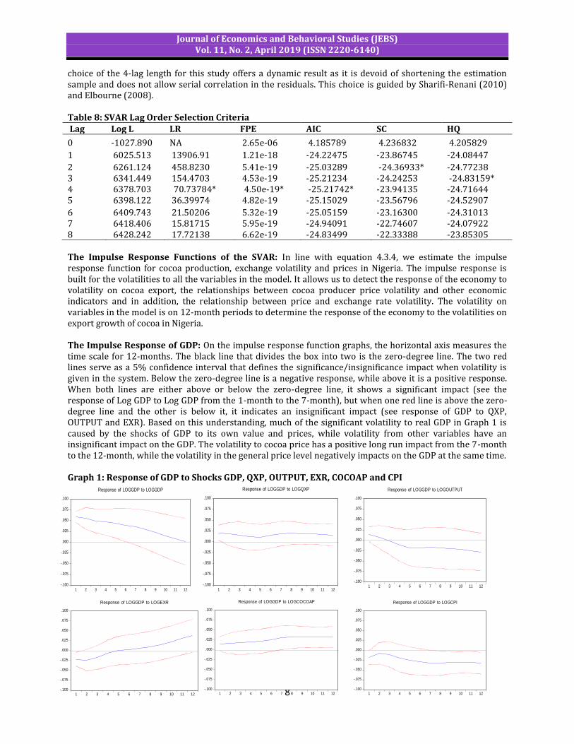
choice of the 4-lag length for this study offers a dynamic result as it is devoid of shortening the estimation sample and does not allow serial correlation in the residuals. This choice is guided by Sharifi-Renani (2010) and Elbourne (2008). Table 8: SVAR Lag Order Selection Criteria Lag Log L LR FPE AIC SC HQ
0 -1027.890 NA 2.65e-06 4.185789 4.236832 4.205829
1 6025.513 13906.91 1.21e-18 -24.22475 -23.86745 -24.08447
2 6261.124 458.8230 5.41e-19 -25.03289 -24.36933* -24.77238 3 6341.449 154.4703 4.53e-19 -25.21234 -24.24253 -24.83159* 4 6378.703 70.73784* 4.50e-19* -25.21742* -23.94135 -24.71644 5 6398.122 36.39974 4.82e-19 -25.15029 -23.56796 -24.52907
6 6409.743 21.50206 5.32e-19 -25.05159 -23.16300 -24.31013 7 6418.406 15.81715 5.95e-19 -24.94091 -22.74607 -24.07922 8 6428.242 17.72138 6.62e-19 -24.83499 -22.33388 -23.85305 The Impulse Response Functions of the SVAR: In line with equation 4.3.4, we estimate the impulse response function for cocoa production, exchange volatility and prices in Nigeria. The impulse response is built for the volatilities to all the variables in the model. It allows us to detect the response of the economy to volatility on cocoa export, the relationships between cocoa producer price volatility and other economic indicators and in addition, the relationship between price and exchange rate volatility. The volatility on variables in the model is on 12-month periods to determine the response of the economy to the volatilities on export growth of cocoa in Nigeria. The Impulse Response of GDP: On the impulse response function graphs, the horizontal axis measures the time scale for 12-months. The black line that divides the box into two is the zero-degree line. The two red lines serve as a 5% confidence interval that defines the significance/insignificance impact when volatility is given in the system. Below the zero-degree line is a negative response, while above it is a positive response. When both lines are either above or below the zero-degree line, it shows a significant impact (see the response of Log GDP to Log GDP from the 1-month to the 7-month), but when one red line is above the zero-degree line and the other is below it, it indicates an insignificant impact (see response of GDP to QXP, OUTPUT and EXR). Based on this understanding, much of the significant volatility to real GDP in Graph 1 is caused by the shocks of GDP to its own value and prices, while volatility from other variables have an insignificant impact on the GDP. The volatility to cocoa price has a positive long run impact from the 7-month to the 12-month, while the volatility in the general price level negatively impacts on the GDP at the same time. Graph 1: Response of GDP to Shocks GDP, QXP, OUTPUT, EXR, COCOAP and CPI
-.100
-.075
-.050
-.025
.000
.025
.050
.075
.100
1 2 3 4 5 6 7 8 9 10 11 12
Response of LOGGDP to LOGGDP
-.100
-.075
-.050
-.025
.000
.025
.050
.075
.100
1 2 3 4 5 6 7 8 9 10 11 12
Response of LOGGDP to LOGQXP
-.100
-.075
-.050
-.025
.000
.025
.050
.075
.100
1 2 3 4 5 6 7 8 9 10 11 12
Response of LOGGDP to LOGOUTPUT
-.100
-.075
-.050
-.025
.000
.025
.050
.075
.100
1 2 3 4 5 6 7 8 9 10 11 12
Response of LOGGDP to LOGEXR
-.100
-.075
-.050
-.025
.000
.025
.050
.075
.100
1 2 3 4 5 6 7 8 9 10 11 12
Response of LOGGDP to LOGCOCOAP
-.100
-.075
-.050
-.025
.000
.025
.050
.075
.100
1 2 3 4 5 6 7 8 9 10 11 12
Response of LOGGDP to LOGCPI
Journal of Economics and Behavioral Studies (JEBS) Vol. 11, No. 2, April 2019 (ISSN 2220-6140)
9
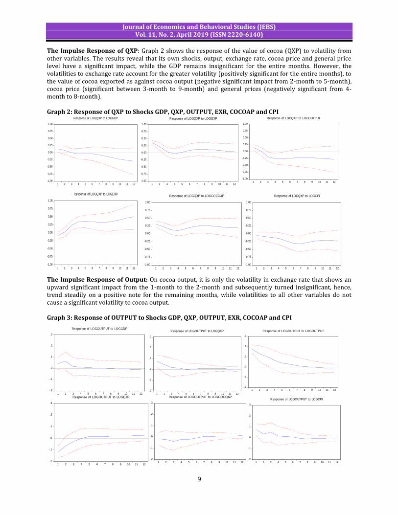
The Impulse Response of QXP: Graph 2 shows the response of the value of cocoa (QXP) to volatility from other variables. The results reveal that its own shocks, output, exchange rate, cocoa price and general price level have a significant impact, while the GDP remains insignificant for the entire months. However, the volatilities to exchange rate account for the greater volatility (positively significant for the entire months), to the value of cocoa exported as against cocoa output (negative significant impact from 2-month to 5-month), cocoa price (significant between 3-month to 9-month) and general prices (negatively significant from 4-month to 8-month). Graph 2: Response of QXP to Shocks GDP, QXP, OUTPUT, EXR, COCOAP and CPI The Impulse Response of Output: On cocoa output, it is only the volatility in exchange rate that shows an upward significant impact from the 1-month to the 2-month and subsequently turned insignificant, hence, trend steadily on a positive note for the remaining months, while volatilities to all other variables do not cause a significant volatility to cocoa output. Graph 3: Response of OUTPUT to Shocks GDP, QXP, OUTPUT, EXR, COCOAP and CPI
-1.00
-0.75
-0.50
-0.25
0.00
0.25
0.50
0.75
1.00
1 2 3 4 5 6 7 8 9 10 11 12
Response of LOGQXP to LOGGDP
-1.00
-0.75
-0.50
-0.25
0.00
0.25
0.50
0.75
1.00
1 2 3 4 5 6 7 8 9 10 11 12
Response of LOGQXP to LOGQXP
-1.00
-0.75
-0.50
-0.25
0.00
0.25
0.50
0.75
1.00
1 2 3 4 5 6 7 8 9 10 11 12
Response of LOGQXP to LOGOUTPUT
-1.00
-0.75
-0.50
-0.25
0.00
0.25
0.50
0.75
1.00
1 2 3 4 5 6 7 8 9 10 11 12
Response of LOGQXP to LOGEXR
-1.00
-0.75
-0.50
-0.25
0.00
0.25
0.50
0.75
1.00
1 2 3 4 5 6 7 8 9 10 11 12
Response of LOGQXP to LOGCOCOAP
-1.00
-0.75
-0.50
-0.25
0.00
0.25
0.50
0.75
1.00
1 2 3 4 5 6 7 8 9 10 11 12
Response of LOGQXP to LOGCPI
-.2
-.1
.0
.1
.2
.3
1 2 3 4 5 6 7 8 9 10 11 12
Response of LOGOUTPUT to LOGGDP
-.2
-.1
.0
.1
.2
.3
1 2 3 4 5 6 7 8 9 10 11 12
Response of LOGOUTPUT to LOGQXP
-.2
-.1
.0
.1
.2
.3
1 2 3 4 5 6 7 8 9 10 11 12
Response of LOGOUTPUT to LOGOUTPUT
-.2
-.1
.0
.1
.2
.3
1 2 3 4 5 6 7 8 9 10 11 12
Response of LOGOUTPUT to LOGEXR
-.2
-.1
.0
.1
.2
.3
1 2 3 4 5 6 7 8 9 10 11 12
Response of LOGOUTPUT to LOGCOCOAP
-.2
-.1
.0
.1
.2
.3
1 2 3 4 5 6 7 8 9 10 11 12
Response of LOGOUTPUT to LOGCPI

Journal of Economics and Behavioral Studies (JEBS) Vol. 11, No. 2, April 2019 (ISSN 2220-6140)
10
The Impulse Response of EXR: The result on the exchange rate exhibits similar but different response as shocks from GDP and OUTPUT. It shows a significant impact in causing volatility from the 1-month to the 2-month. The volatilities to general price level significantly cause volatility in exchange rate from the 2-month to the 5-month, which is from its own shock (response of log EXR to log EXR) and accounts for much of the volatilities. It remains positively significant for the entire analysed period. Graph 4: Response of EXR to Shocks GDP, QXP, OUTPUT, EXR, COCOAP and CPI The Impulse Response of COCOAP: In Graph 5, the shocks from GDP do not have a significant impact on cocoa price for the whole months, while shocks to value of cocoa only have a significant impact from the 1-2 months. The volatilities to output negatively cause volatility in cocoa price from the 2-5 months. The volatilities to exchange rate show a great impact from the 2-month to the 12-month before it dies off, causing volatility in cocoa price. In addition, the general price level also has a negative significant impact on cocoa price from the 1-month to the 8-month. Graph 5: Response of COCOAP to Shocks GDP, QXP, OUTPUT, EXR, COCOAP and CPI
-.8
-.6
-.4
-.2
.0
.2
.4
.6
.8
1 2 3 4 5 6 7 8 9 10 11 12
Response of LOGEXR to LOGGDP
-.8
-.6
-.4
-.2
.0
.2
.4
.6
.8
1 2 3 4 5 6 7 8 9 10 11 12
Response of LOGEXR to LOGQXP
-.8
-.6
-.4
-.2
.0
.2
.4
.6
.8
1 2 3 4 5 6 7 8 9 10 11 12
Response of LOGEXR to LOGOUTPUT
-.8
-.6
-.4
-.2
.0
.2
.4
.6
.8
1 2 3 4 5 6 7 8 9 10 11 12
Response of LOGEXR to LOGEXR
-.8
-.6
-.4
-.2
.0
.2
.4
.6
.8
1 2 3 4 5 6 7 8 9 10 11 12
Response of LOGEXR to LOGCPI
-.8
-.6
-.4
-.2
.0
.2
.4
.6
.8
1 2 3 4 5 6 7 8 9 10 11 12
Response of LOGEXR to LOGCOCOAP
-1.00
-0.75
-0.50
-0.25
0.00
0.25
0.50
0.75
1.00
1 2 3 4 5 6 7 8 9 10 11 12
Response of LOGCOCOAP to LOGGDP
-1.00
-0.75
-0.50
-0.25
0.00
0.25
0.50
0.75
1.00
1 2 3 4 5 6 7 8 9 10 11 12
Response of LOGCOCOAP to LOGQXP
-1.00
-0.75
-0.50
-0.25
0.00
0.25
0.50
0.75
1.00
1 2 3 4 5 6 7 8 9 10 11 12
Response of LOGCOCOAP to LOGOUTPUT
-1.00
-0.75
-0.50
-0.25
0.00
0.25
0.50
0.75
1.00
1 2 3 4 5 6 7 8 9 10 11 12
Response of LOGCOCOAP to LOGEXR
-1.00
-0.75
-0.50
-0.25
0.00
0.25
0.50
0.75
1.00
1 2 3 4 5 6 7 8 9 10 11 12
Response of LOGCOCOAP to LOGCOCOAP
-1.00
-0.75
-0.50
-0.25
0.00
0.25
0.50
0.75
1.00
1 2 3 4 5 6 7 8 9 10 11 12
Response of LOGCOCOAP to LOGCPI

Journal of Economics and Behavioral Studies (JEBS) Vol. 11, No. 2, April 2019 (ISSN 2220-6140)
11
The Impulse Response of CPI: The response of the general price level (CPI) from GDP, QXP and EXR does not show any significant impact on the general price level for the whole months, while shocks to output and cocoa price only have a significant impact in the 1-month in causing volatility in the general price level. The volatility in output positively reduces prices, while cocoa price negatively increases prices. This shows that volatility in both cocoa output production and cocoa price have an impact on general price level in the economy, though within a short period of time. Graph 6: Response of CPI to Shocks GDP, QXP, OUTPUT, EXR, COCOAP and CPI Summary of the Findings with Empirical Comparisons in Nigeria: The aim of this study was to examine the export function of cocoa production and determines the effect of price and exchange rate volatility on cocoa export in Nigeria. After estimating the and equations, the estimated model passes several residual diagnostic checks including unit root test, lag selections, structural breakpoints test, structural imposition of restrictions and orthogonalised impulse responses analyses. Firstly, the OLS results for the exports supply model of cocoa showed that all the variables were significant in determining the impacts of the value of cocoa production in Nigeria. The price of cocoa on the international market and the value of exchange rates play a significant role on cocoa exports growth in Nigeria. This is in line with Onoja et al. (2012) who carried a study on “the profitability and yield determinants in Nigeria cocoa farm”. They recommended that cocoa farming be encouraged to create jobs and reduce poverty, as well as microfinance banks and agricultural agencies to provide farmers with access to credit. Farmers need to be trained on the most effective ways of production to guarantee sustainable cocoa production in Nigeria. In addition, the results are in line with Verter and Bečvářová (2014) who used the Johansen cointegration and OLS regression methods to analyzed cocoa export in Nigeria. Finally, the OLS results provide a positive relationship between cocoa export and cocoa prices, exchange rates and quantity of cocoa export (significant at 5%). Likewise, the SVAR analysis shows that much of the results from the impulse response graphs on the volatility to GDP are from the global price of cocoa on the international market. A rise in the price of cocoa will increase cocoa production and export growth in Nigeria. This view supports Idowu et al. (2007) who showed that the significant rise in the total cocoa output production can be attained through a combination of a sustained increase in real producer price, local currency stability and real supply of chemical fertilizer. Additionally, the response of the value of cocoa production shows that the volatilities from the output, exchange rate, cocoa price and general price level have a significant impact, while the GDP remains insignificant for the whole months. The result reveals that the volatilities to exchange rate accounts for the greater volatility (positively significant for the entire months) to the value of cocoa exported as against other variables in the model. This echoes Abolagba et al.’s (2010) findings which showed that the Naira exchange rate volatility reduced non-oil exports by 3.65%, while the US dollar volatility increased export of non-oil (cocoa inclusive) in Nigeria.
-0.4
-0.2
0.0
0.2
0.4
0.6
0.8
1.0
1 2 3 4 5 6 7 8 9 10 11 12
Response of LOGCPI to LOGGDP
-0.4
-0.2
0.0
0.2
0.4
0.6
0.8
1.0
1 2 3 4 5 6 7 8 9 10 11 12
Response of LOGCPI to LOGQXP
-0.4
-0.2
0.0
0.2
0.4
0.6
0.8
1.0
1 2 3 4 5 6 7 8 9 10 11 12
Response of LOGCPI to LOGOUTPUT
-0.4
-0.2
0.0
0.2
0.4
0.6
0.8
1.0
1 2 3 4 5 6 7 8 9 10 11 12
Response of LOGCPI to LOGEXR
-0.4
-0.2
0.0
0.2
0.4
0.6
0.8
1.0
1 2 3 4 5 6 7 8 9 10 11 12
Response of LOGCPI to LOGCOCOAP
-0.4
-0.2
0.0
0.2
0.4
0.6
0.8
1.0
1 2 3 4 5 6 7 8 9 10 11 12
Response of LOGCPI to LOGCPI
Journal of Economics and Behavioral Studies (JEBS) Vol. 11, No. 2, April 2019 (ISSN 2220-6140)
12
However, for the impulse response analysis of cocoa output, only the volatility of exchange rate shows a significant impact. This finding reflects the view of Nwachuku et al. (2010) who revealed that world export volume, exchange rates and cocoa output were determinants of cocoa export in Nigeria. Overall, the results from this study concur with Essien et al. (n.d) and Adeyeye (2012) that the exchange rate and prices are very crucial to the export growth of cocoa in Nigeria. This is because the price of cocoa is still exogenously determined from the world market, hence, both forces of demand and supply greatly impact on cocoa output growth. The exchange rate has impacted positively on cocoa export in Nigeria; hence, as a policy recommendation, there should be a free market determination of exchange rate for export of cocoa in Nigeria. The repeated intervention by the International Monetary Fund (IMF) 2004 should be discouraged, as it will only increase poverty and reduce output in the country. A weaker exchange rate of the naira will lead to an increase in prices domestically, which can propagate to other sectors of the economy (especially on agricultural products). On the other hand, a stronger exchange rate of naira will reduce prices domestically, and later stabilize the exchange rates and increase cocoa output growth. Finally, as a policy guide, it is recommended that the forces of demand and supply should be allowed to fully determine the value of exchange rates in Nigeria. References
Abang, S. O. & Ndifon, H. M. (2002). Analysis of world cocoa production trends and their production share
coefficients (1975-1996). Nigeria Agricultural Journal, 33(1), 10-16. Abolagba, E. O., Onyekwere, N. C., Agbonkpolor, B. N. & Umar, H. Y. (2010). Determinants of agricultural
exports. Journal of Human Ecology, 29(3), 181. Acemoglu, D., Johnson, S., Robinson, J. & Thaicharoen, Y. (2003). Institutional causes, macroeconomic
symptoms: volatility, crises and growth. Journal of monetary economics, 50(1), 49-123. Adeyeye, C. T. (2012). Cocoa Production and Price Stability: An Industrial Relations Perspective. Accessed on,
1(10). Adubi, A. A. & Okunmadewa, F. (1999). Price, exchange rate volatility and Nigeria's agricultural trade flows: A
dynamic analysis (No. RP_087). African Economic Research Consortium. Aizenman, J. & Marion, N. P. (1993). Policy uncertainty, persistence and growth*. Review of international
economics, 1(2), 145-163. Aizenman, J. & Pinto, B. (Eds.). (2005). Managing Economic Volatility and Crises: A Practitioner's Guide.
Cambridge University Press. Aliyu, S. U. R. (2008). Exchange rate volatility and export trade in Nigeria: an empirical investigation. Applied
Financial Economics, 20(13), 1071-1084. Amisano, G. & Giannini, C. C. (1997). Topics in structural VAR econometrics. Babula, R. A., Ruppel, F. J. & Bessler, D. A. (1995). US corn exports: the role of the exchange rate. Agricultural
Economics, 13(2), 75-88. Bala, D. A. & Asemota, J. O. (2013). Exchange-rates volatility in Nigeria: Application of GARCH models with
exogenous break. CBN Journal of Applied Statistics, 4(1), 89-116. Bradshaw, G. W. & Orden, D. (1990). Granger causality from the exchange rate to agricultural prices and
export sales. Western Journal of Agricultural Economics, 100-110. Braun, J. V. & Tadesse, G. (2012). Global food price volatility and spikes: an overview of costs, causes, and
solutions. ZEF-Discussion Papers on Development Policy, (161). Buckle, R. A., Kim, K., Kirkham, H., McLellan, N. & Sharma, J. (2007). A structural VAR business cycle model for
a volatile small open economy. Economic Modelling, 24(6), 990-1017. Chou, W. L. (2000). Exchange rate variability and China's exports. Journal of Comparative Economics, 28(1),
61-79. Dehn, J., Gilbert, C. L. & Varangis, P. (2005). Agricultural commodity price volatility. Managing Economic
Volatility and Crises: A Practitioner’s Guide, 137-85. Demetriades, P. & Fielding, D. (2012). Information, institutions, and banking sector development in West
Africa. Economic Inquiry, 50(3), 739-753. Denbaly, M. & Torgerson, D. (1992). Macroeconomic determinants of relative wheat prices: integrating the
short run and long run. Journal of Agricultural Economics Research, 44(2), 27-35. Dungey, M. & Fry, R. (2007). The Identification of Fiscal and Monetary Policy in a Structural VAR. CFAP,
Journal of Economics and Behavioral Studies (JEBS) Vol. 11, No. 2, April 2019 (ISSN 2220-6140)
13
University of Cambridge and CAMA, Australian National University [unpublished) Dungey, M. & Fry, R. (2009). The identification of fiscal and monetary policy in a structural VAR. Economic
Modelling, 26(6), 1147-1160. Elbourne, A. (2008). The UK housing market and the monetary policy transmission mechanism: An SVAR
approach. Journal of Housing Economics, 17(1), 65-87. Enders, W. (2004). Applied Econometric Time Series. Essien, E. B., Dominic, A. O. & Sunday, E. R. (n.d). Effects of Price and Exchange Rate Fluctuations on
Agricultural Exports in Nigeria. Frimpong, P. B. (2012). Population Health and Economic Growth: Panel Cointegration Analysis in Sub-
Saharan Africa. Master’s thesis at Lund University. Gilbert, C. (2006). Trends and volatility in agricultural commodity prices. Agricultural Commodity Markets
and Trade: New Approaches to Analyzing Market Structure and Instability, 31-60. Green, W. H. (2002). Econometric Analysis. Fifth Edition Prentice Hall, Upper Saddle, River, New Jersey. Goyal, A., Arora, S. (2010). A GARCH analysis of exchange rate volatility and the effectiveness of central bank
actions, Indira Gandhi Institute of Development Research, Mumbai, 1–19. Hanson, B. E. (2002). Tests for parameter instability in regressions with I (1) processes. Journal of Business &
Economic Statistics, 20(1), 45-59. Idowu, E. O., Osuntogun, D. A. & Oluwasola, O. (2007). Effects of market deregulation on cocoa (Theobroma
cacao) production in Southwest Nigeria. African Journal of Agricultural Research, 2(9), 429-434. IFPRI. (2011). 2011 Global Food Policy Report, Washington DC: International Food Policy Research Institute. IMF. (1984). Exchange Rate Volatility and World Trade. A Study by the Research Department of IMF,
occasional paper No. 28, Washington DC, IMF. IMF. (2004). A New Look at Exchange Rate Volatility and Trade Flows. Occasional Paper No. 235. Johnson, P. R., Grennes, T. & Thursby, M. (1977). Devaluation, foreign trade controls, and domestic wheat
prices. American Journal of Agricultural Economics, 59(4), 619-627. Ishibashi, S. (2012). The Segmentation of Loan Interest Rates by Regional Financial Institutions: A Panel
Cointegration Analysis. International Review of Business Research Papers, 8(5), 95- 110. Kandilov, I. T. (2008). The effects of exchange rate volatility on agricultural trade. American Journal of
Agricultural Economics, 90(4), 1028-1043. Kiptui, M. (2007, July). Does the exchange rate matter for Kenya’s exports? A bounds testing approach.
Conference, of African Econometric Society. Kutu, A. A., Nzimande, N. P. & Msomi, S (2017). Effectiveness of Monetary Policy and the Growth of Industrial
Sector in China. Journal of Economics and Behavioral Studies, 9(3), 46-59. McCoy, D. (1997). How useful is Structural VAR Analysis for Irish economics? (No. 2/RT/97). Central Bank of
Ireland. Mehare, A. & Edriss, A. K. (2012). Evaluation of Effect of Exchange Rate Variability on Export of Ethiopia’s
Agricultural Product: Case of Oilseeds. Evaluation, 3(11). Moon, H. R. & Perron, B. (2004). Testing for a unit root in panels with dynamic factors. Journal of
Econometrics, 122(1), 81-126. Ngalawa, H. & Kutu, A. A. (2017). Modelling exchange rate variations and global shocks in Brazil. Zbornik
Radova Ekonomskog fakulteta u Rijeci: časopis za ekonomsku teoriju ipraksu, 35(1), 73-95. Ngalawa, H. & Viegi, N. (2011). Dynamic effects of monetary policy shocks in Malawi. South African Journal of
Economics, 79(3), 224-250. Nkang, N. M., Abang, S. O., Akpan, O. E. & Offem, K. J. (2006). Cointegration and error correction modelling of
agricultural export trade in Nigeria: The case of cocoa. Journal of Agriculture and Social Sciences, 2(4), 249-255.
Nwachuku, I. N., Agwu, N., Nwaru, J. & Imonikhe, G. (2010). Competitiveness and determinants of cocoa export from Nigeria. Report and Opinion, 2(7), 51-54.
Okunmadewa, F. (1999). Livestock industry as a tool for poverty alleviation. Nigerian Journal of Animal Science, 2(2).
Onoja, A. O., Deedam, N. J. & Achike, A. I. (2012). Profitability and yield determinants in Nigeria cocoa farms: Evidence from Ondo State. Journal of Sustainable Development in Africa, 14(4), 172-183.
Oyinlola, M. A. (2008). Exchange Rate and Disaggregated Import Prices in Nigeria. Exchange Rate and Disaggregated Import Prices in Nigeria. Journal of Economic and Monetary Integration, 9, 89-126.

Journal of Economics and Behavioral Studies (JEBS) Vol. 11, No. 2, April 2019 (ISSN 2220-6140)
14
Pesaran, H. H. & Shin, Y. (1998). Generalized impulse response analysis in linear multivariate models. Economics Letters, 58(1), 17-29.
Ramaswamy, R. & Sloek, T. (1998). The real effects of monetary policy in the European Union: What are the differences? Staff Papers, 45(2), 374-396.
Ramey, G. & Ramey, V. A. (1995). Cross-country evidence on the link between volatility and growth (No. w4959). National Bureau of economic research.
Schwartz, N. E. (1986). The consequences of a floating exchange rate for the US wheat market. American Journal of Agricultural Economics, 68(2), 428-433.
Sharifi-Renani, H. O. S. E. I. N. (2010). A structural VAR approach of monetary policy in Iran. In International Conference on Applied Economics–ICOAE (p. 631).
Stock, J. H. & Watson, M. W. (2005). Implications of dynamic factor models for VAR analysis (No. w11467). National Bureau of Economic Research.
Tshibaka, T. (1997). Effects of domestic economic policies and external factors on export prices and their implications for output and income in Cameroon. AERC Final Report, Nairobi: AERC.
Verter, N. & Bečvářová, V. (2014). Analysis of Some Drivers of Cocoa Export in Nigeria in the Era of Trade Liberalization. AGRIS on-line Papers in Economics and Informatics, 6(4).
Villanueva, J. L. J. & Sarker, R. (2009, August). Exchange Rate Sensitivity of Fresh Tomatoes Imports from Mexico to the United States. In Contributed Paper prepared for presentation at the International Association of Agricultural Economists Conference, Beijing, China, August 16 (Vol. 22, p. 2009).
Weersink, A., Hailu, G., Fox, G., Meilke, K. & von Massow, M. (2008). The world food crisis: Causes and the implications for Ontario agriculture (No. 46503).
Journal of Economics and Behavioral Studies (JEBS) Vol. 11, No. 2, April 2019 (ISSN 2220-6140)
15
The Nexus between Consumer Confidence and Economic Growth in South Africa: An ARDL Bounds Testing Approach
Khayelihle Madlopha
University of Zululand, Department of Economics, KwaDlangezwa, South Africa [email protected]
Abstract: Consumption expenditure contributed a total of 2.2% to economic growth in 2017. Hence, the South African economy is consumption driven. Therefore, there is a need to understand the growth-economic confidence relationship within the South African context. In this spirit, this paper set to explore the short- and long-run relationship between consumer confidence and economic growth in South Africa for the sample period 1994Q1 to 2017Q4. The method applied, chiefly because our variables were I (0) and I (1) and that we sought short- and long-run estimates were the Autoregressive Distributed Lag (ARDL) model using the bounds testing procedure. The results showed that consumer confidence contributed about 0.025% to economic growth in the short-run, and about 0.4% in the long-run. The results suggest that boosting consumer confidence should be keys for South African policy-makers to boost growth in the short- and long-run. In particular, we recommend policy certainty and political stability as some of the ways to attract consumer confidence. Keywords: Consumer confidence, consumption expenditure, economic growth, ARDL, South Africa
1. Introduction South Africa’s economic growth has been sluggish and discomforting since the 2008 crisis. The country’s economic growth exhibits hysteresis effects1: it has not been able to return to its pre-crisis average level which hovered around 4%2. The slow growth is partly responsible for the high unemployment rate and inequality. Studies (for example, see: Maduku and Kaseeram (2018)) found that economic growth is a determinant of Foreign Direct Investment (FDI) in South Africa, thus suggesting that low growth is also responsible for the downward trend in FDI that the country has been experiencing. Such low growth over years has not been a problem only for the South African economy, but also its citizens (Harmse, 2006). There is thus is an urgent need for the country to set itself on a higher growth path. Amid, the South African government aspires to achieve 5% growth rate in order to significantly reduce the high unemployment rate and tackle inequality. Consequently, the government has sought many avenues through which to achieve high and sustainable economic growth, with the attraction of FDI the most favoured approach. However, the yet moderate economic growth evidence that the country has failed to set itself on a higher growth path. This is even after many attempts, specifically economic policies such as the Reconstruction and Development Program (RDP) (1994) and the relatively recent National Development Plan (NDP) (2013). Previous studies which looked at how South Africa can set itself on a higher growth path include Lewis (2001), Faulkner and Loewald (2008), Faulkner, Loewald and Makrelov (2013), Bernstein, de Kadt, Roodt and Schirmer (2014), Nattrass (2014) and Leowald (2018). The weakness of these studies is that they replicated previous studies by using the same variables, notably fiscal, monetary and social (poverty and inequality) variables. Overcoming the weakness of these studies, we contribute3 to the existing body of
1 In Physical Science, ‘hysteresis’ is the inability of an object to revert to its initial position even after the
effects of an external force is removed (Ball and Mankiw, 2002). Contextually, it refers to the inability of South Africa’s growth to return to its pre-crisis levels even after the crisis. 2 The average growth rate was 5% between 1994 and 2003, and 5% between 2004 and 2007 (South African Reserve Bank, 2009). 3 To the best of our knowledge, the relationship between economic confidence and economic growth has not
been explicitly studied in South Africa.

Journal of Economics and Behavioral Studies (JEBS) Vol. 11, No. 2, April 2019 (ISSN 2220-6140)
16
literature on how South Africa can set itself on a higher growth path by introducing a new variable into analysis: consumer confidence4. There are chiefly 2 motivations for why consumer confidence is a variable worth incorporating into the analysis of economic growth. Firstly, economic theory justifies the importance of consumer expenditure – which is strongly driven by consumer confidence–on economic growth. Keynes (1936) stressed the importance of consumption expenditure on economic growth. He held that higher consumption expenditure led to higher aggregate demand, output and economic growth, which increased labour demand and employment. Thus, it is easy to see the macroeconomic importance of consumption expenditure and, by extension, consumer confidence, in the South African economy. Secondly, consumption expenditure has historically contributed a large portion to annual growth in South Africa, and in 2017 it contributed 2.2% (Statistics South Africa, 2018), which was the biggest contribution of all expenditure components of Gross Domestic Expenditure (GDE). To that extent, the South African economy is consumption driven and the relationship between consumer confidence and economic growth ought to be examined. Notwithstanding the importance of this relationship, a few studies have disappointedly explored the relationship between consumer confidence and economic growth (see: Matsusaka & Sbordone, 1995; Utaka, 2003; Sergeant, 2011; Islam and Mumtaz, 2016). Rather, most studies utilised consumer confidence in predicting consumer expenditure (Leeper, 1992; Howrey, 2001; Ludvigson, 2004) and oil prices (Praet and Vuchelen, 1989; Mehra and Petersen, 2005; Güntner and Linsbauer, 2018), asset pricing (Kim and Oh, 2009; Lemmon & Portniaguina, 2006; Charoentook, 2005), and stock market analysis (Jansen and Nahuis, 2003; Otoo, 1999; Fisher and Statman, 2003). In this backdrop, this paper aims to explore the short-run and long-run nexus between consumer confidence and economic growth in South Africa. The rest of the paper is set out as follows: Section 2 reviews relevant literature, Section 3 covers data and methodology, Section 4 covers results and analysis, while Section 5 concludes. 2. Literature Review The relationship between economic growth and aggregate spending has a long history in macroeconomics. This relationship attracted macroeconomists after Keynes (1936) wrote the General Theory of Employment, Interest and Money (‘The General Theory’). In the wake of the great depression, Keynes (1936) argued that an optimal solution to boost economic activity was to reduce taxes and increase government spending to boost aggregate spending. The rationale was that lowering taxes would spur higher household consumption spending as these economic agents enjoyed higher disposable incomes. As the government spent, it would increase demand for goods and services in the economy and thereby create employment5. The culmination of these would be higher economic activity and lower unemployment, thus rescuing the economy from the recession. Attributed to Keynes (1936) is the term ‘animal spirits’ coined in the General Theory. Put simply, the term referred to the extent to which consumers were determined to consume or purchase goods and services. To the extent that such determination to consume is highly dependent on the confidence of consumers about the future state of the economy (i.e. consumer confidence). It is clear that consumer confidence entered macroeconomics in earlier years than we think. However, it had not been explicitly coined and studied. Keynesianism proved itself, prominent and successful in many economies, and the importance of consumption expenditure on economic growth was appreciated. This led to attempts directed at measuring economic confidence6. These attempts led to the development of consumer confidence index (CCI), which gauges consumer confidence. The CCI has been used to understand the relationship between consumer confidence and various macroeconomic and financial markets variables. As stated before, a few studies have investigated the relationship between consumer confidence and economic
4 Consumer confidence refers to the extent to which households or individual consumers are confident or optimistic about the performance or state of an economy. 5 This was summarized by the aggregate consumption function, which represents a positive relationship between aggregate consumption expenditure and output. 6 Economic confidence is an umbrella term which includes consumer and business confidence, with business confidence measuring the optimism businesses have about an economy.
Journal of Economics and Behavioral Studies (JEBS) Vol. 11, No. 2, April 2019 (ISSN 2220-6140)
17
growth. On the other hand, most studies investigate consumer confidence in the context of financial markets. One such study is Çelik and Özerkek (2009), who employed a panel cointegration analysis to understand the relationship between consumer confidence, real exchange rate the performance of stock market, interest rates, and personal consumption. The study was in the context of 9 European economies7. A long-run positive relationship between consumer confidence and the other variables was found. A similar study by Çelik, Aslanoglu and Deniz (2010) was conducted, and a cointegration relationship between consumer confidence and interest rates, exchange rate and the stock market existed. In particular, consumer confidence had a positive effect on these variables. Çelik, Aslanoglu and Uzin (2010) studied the link between consumer confidence and industrial output in 9 emerging economies8. Also aided by panel cointegration, the authors also examined how consumer confidence related to the stock market index. Similar to Çelik and Özerkek (2009) and Çelik, Aslanoglu and Deniz (2010), the authors found a positive, long-run impact of consumer confidence on the performance of the stock exchange. Interestingly, the study found a positive impact on consumer confidence of industrial output. This suggests that consumer confidence had positive effects on the economies of these countries, as industrial output is synchronized with economic growth. These results were similar to those of Li (2010), who concluded that consumer confidence Granger-caused industrial output in China. One of the few studies that examine the relationship between consumer confidence and economic growth, Sergeant, Lugay and Dookie (2011) examined the context of Jamaica and Trinidad and Tobago. The results concurred with those of Oduh, Oduh and Ekeocha (2012), Islam and Mumtaz (2016) and Ibrahim, Bawa, Abdullahi, Didigu and Mainasara (2015), who also found that consumer confidence had a positive and significant impact on economic growth. However, the effect was insignificant for Jamaica. While Çelik et al. (2010) included South Africa in the panel of countries, studying a country as part of a panel has its weaknesses. Panel analysis is weakened by unobserved heterogeneity between countries. After all, no matter how similar or integrated economies are, heterogeneous economic and social structures always present a certain level of unobserved heterogeneity. Also, panel analyses generally omit country-specific policies or optimal policy recommendations. This was also the case with Çelik et al. (2010). Being a single-country analysis, this study addresses the above-mentioned weaknesses of panel analyses. 3. Data and Methodology Data: The sample period was guided by the availability of the unemployment rate data and ranges from 1994Q1 to 2017Q4, with some data interpolated because the real exchange rate, unemployment rate and gross fixed capital were not available on quarterly basis. Given that the sample period starts from the first quarter of the year in which democracy dawned on South Africa, the analysis can be interpreted as the relationship between consumer confidence and economic growth in a democratic society. Our study differs slightly from Islam et al. (2016) by that we use unemployment than employment rate in our analysis, as Statistics South Africa reports the unemployment than the employment rate and unemployment rate statistics make the news frequently and are given more attention in South Africa than employment. The other difference is that we left out real interest rates as a regressor, due to data unavailability. The data for consumer confidence was sourced from the Bureau of Economic Research (BER) and the other data from the South African Reserve Bank (SARB). As a result, Real GDP (G) is used as a dependent variable and independent variables are consumer confidence index (CCI), real effective exchange rate (REER), gross fixed capital formation (GFCF) and unemployment rate (UNE). The real exchange rate and gross fixed capital formation were converted to percentages for analysis purpose. CCI was not logged as it had many negative values. Method and Model Specification: The empirical method applied in this paper is the Autoregressive Distributed Lag (ARDL) bounds testing procedure proposed by Pesaran, Shin and Smith (2001). There are 3 reasons behind this. Firstly, the model – unlike the Johansen test of cointegration which requires that all variables be I (1) – is applicable in cases similar to the present one, where the data is a mixture of I (0) and I
7 Denmark, France, Germany, Ireland, Italy, Netherlands, Portugal, Spain, and the United Kingdom 8 Brazil, China, Mexico, Poland, South Africa and Turkey

Journal of Economics and Behavioral Studies (JEBS) Vol. 11, No. 2, April 2019 (ISSN 2220-6140)
18
(1) variables (see the discussion on stationary tests below). Secondly, the ARDL model performs better even in the presence of the problem of endogeneity, which is a possible threat to our data as most variables that affect economic growth were parsimoniously omitted. Lastly, with its ability to estimate both short-run and long-run estimates, the model allows us to achieve our objective of examining the relationship between consumer confidence and economic growth in the short- and long-run periods. Diagnostic checks were done, and we found no problem with heteroscedasticity, but with autocorrelation. The ARDL bounds testing procedure begins with an unconstrained error correction representation: ∆Y = α0 + α1Yt – 1 + α2CCIt – 1 + α3LREERt – 1 + α4LGFCFt – 1 + α5UNEt – 1 +
+ +
+
+ εt …. (1)
t = 1994Q1, …, 2017Q4 Where ∆ is the first difference operator, L indicates logarithmic of a variable, and εt the error term. Lag lengths for regressors are automatically selected by Akaike Information Criterion (AIC), as AIC performs better than other alternatives (Lemmon, 2006). In performing the bounds testing procedure, we first estimate equation (1) by the OLS method and then test for the hypothesis of joint significance of lagged level variable parameters using an F-test. The assumption of no trend and intercept is imposed. Pesaran et al. (2001) provide two sets of estimates for the upper and lower bounds to be used in bounds testing. An F-statistic which lies below (upper) the lower bound signals the non- existence (existence) of a long-run relationship, while an F-statistic which lies in between the upper and lower bounds is inconclusive. H0: α1 = α2 = α3 = α4 = α5 = 0 is the null hypothesis of no long-run relationship, which is tested against the alternative hypothesis H1: α1 ≠ α2 ≠ α3 ≠ α4 ≠ α5 ≠ 0. If a long-run relationship exists, then equation (1) can be represented as an error correction: ∆log Yt = c +
+ +
+
+ λECTt – 1 + ε1t …. (2) Where, lagged by one quarter, ECTt – 1 is an error correction term that corrects short-run disequilibria to achieve a long-run equilibrium. 4. Results and Discussion As stated before, if the bounds test indicates a cointegrating relationship, then it suggests the existence of a long-run relationship between variables of interests. In this Section, we therefore first present results of the bounds test and follow with short-run and long-run estimates. Bounds Testing: The following results were obtained, where Fg indicates the F-statistic obtained when growth was a dependent variable. F statistic 5% critical value 1% critical value Conclusion Bound bounds I (0) I (1) I (0) I (1) Fg =3.852452 2.69 3.83 3.31 4.63 Cointegrated Fg is above the upper bound at 5%, thus evidencing that a long-run relationship exists at 5% level of significance. Short-Run Estimates: To obtain short-run estimates, we estimated an OLS model. After checking stationarity using the Philipps-Peron test, all variables were differed once to satisfy stationarity, except for consumer confidence, which was I (0). Diagnostic checks were done, and we found no problem with heteroscedasticity, but with autocorrelation. To correct for autocorrelation, we added a one-quarter lag of the dependent as a regressor. After this, autocorrelation was corrected for. For reasons outlined in the next subsection, 3 dummy variables were incorporated in the model. The data was normality distributed, according to the Jacque-Bera test. The Ramsey RESET Test indicated no model misspecification.

Journal of Economics and Behavioral Studies (JEBS) Vol. 11, No. 2, April 2019 (ISSN 2220-6140)
19
Table 1: Short-Run Estimates Variable Coefficient Std. Error t-Statistic Prob. C 0.001973 0.001269 1.554342 0.1238 DUNE -0.000560 0.000617 -0.908476 0.3662 DLGFCF 0.037336 0.014165 2.635777 0.0100 DLREER -0.010388 0.011717 -0.886506 0.3778 CCI 0.000225 6.43E-05 3.492290 0.0008 DIT 0.005068 0.001742 2.909170 0.0046 DCRISIS -0.003902 0.001689 -2.310414 0.0233 DGFR 0.000725 0.001417 0.511812 0.6101 DG(-1) 0.281638 0.097949 2.875366 0.0051 R-squared 0.438593 Mean dependent var 0.007077 Adjusted R-squared 0.385754 S.D. dependent var 0.005821 S.E. of regression 0.004562 Akaike info criterion -7.851346 Sum squared resid 0.001769 Schwarz criterion -7.607839 Log-likelihood 378.0133 Hannan-Quinn criteria. -7.752987 F-statistic 8.300656 Durbin-Watson stat 1.970327 Prob(F-statistic) 0.000000 As reported in Table 1 above, consumer confidence contributes about 0.0225% to economic growth in the short-run. The results concur with results reported by Sergeant et al. (2011), Oduh et al. (2012), Ibrahim et al. (2015) and Islam and Mumtaz (2016), who find a positive effect of consumer confidence on economic growth. The announcement of the inflation targeting regime boded well for short-run growth, with an increase of 0.5% in growth. This was through expectations of a more effectively managed inflation, which was good for forecasting and real returns for investors. A one percentage-point increase in fixed investment was associated with a 0.03% increase in short-run growth. This possibly happened through the channel of increased short-run employment. Growth in the previous quarter contributed 0.28% to growth in the current period. Unemployment was insignificant in explaining short-run growth, and the aftermath of the 2008/2009 crisis, 2000s crisis and exchange rate were found to have no impact on economic growth in the short-run. Long-Run Estimates: We employed the Error Correction Model to estimate the long-run estimate. However, the error correction term was positive. We suspected some issues with the model and did checks on possible sources of the issues. Initially, we had excluded the trend in the model. After including the trend in the model, it was significant, thus signalling that it should be included in the model. Yet, the error correction term was positive. We did further checks and tested for structural breaks using the Multiple Breakpoint Test. The results indicated that in 1999q1, 2003q4 and 2010q1 there were breaks or changes in the structures. We assert that the 1999q1 break is attributed to expectations of the change in monetary policy regime; that is, introduction of the formal inflation targeting. We believe the ‘2000s recessions’ – which affected the European Union between 2000 and 2001 and the US between 2002 and 2003 – had spill-over effects to South Africa, as the US and European Union had relatively heavier ties with South Africa. We attribute the 2010q1 break to the aftermath of the great financial crisis. To incorporate the breaks in the model, we added dummy variables for these break periods. Dit, Dcrisis and Dgfr are for the respective periods and breaks discussed 0 for the periods before breaks and 1 after. After this, the error correction term had the expected sign and magnitude and was significant. The model was dynamically stable, with the Ramsey RESET Test indicating no model misspecification. We found that about 16% of short-run disequilibrium is corrected within one quarter. This signifies a moderate adjustment to the steady-state. Given the significance of the speed of adjustment, however, we welcome the results.
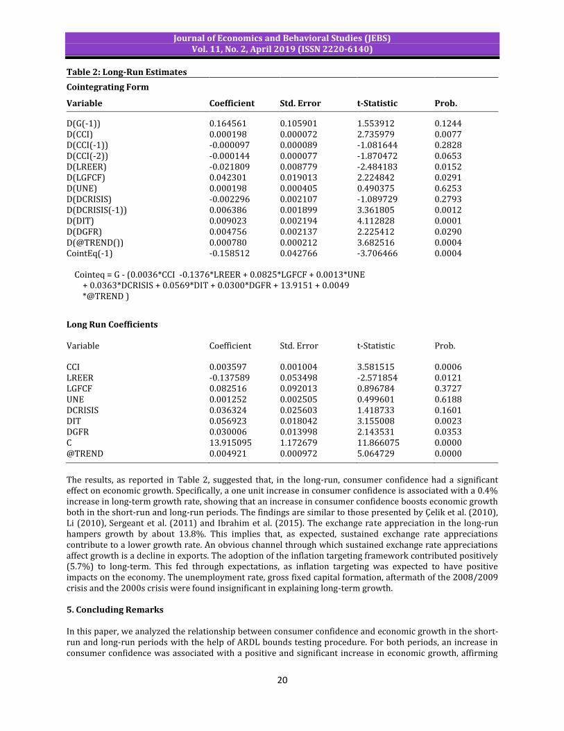
Journal of Economics and Behavioral Studies (JEBS) Vol. 11, No. 2, April 2019 (ISSN 2220-6140)
20
Table 2: Long-Run Estimates Cointegrating Form Variable Coefficient Std. Error t-Statistic Prob. D(G(-1)) 0.164561 0.105901 1.553912 0.1244 D(CCI) 0.000198 0.000072 2.735979 0.0077 D(CCI(-1)) -0.000097 0.000089 -1.081644 0.2828 D(CCI(-2)) -0.000144 0.000077 -1.870472 0.0653 D(LREER) -0.021809 0.008779 -2.484183 0.0152 D(LGFCF) 0.042301 0.019013 2.224842 0.0291 D(UNE) 0.000198 0.000405 0.490375 0.6253 D(DCRISIS) -0.002296 0.002107 -1.089729 0.2793 D(DCRISIS(-1)) 0.006386 0.001899 3.361805 0.0012 D(DIT) 0.009023 0.002194 4.112828 0.0001 D(DGFR) 0.004756 0.002137 2.225412 0.0290 D(@TREND()) 0.000780 0.000212 3.682516 0.0004 CointEq(-1) -0.158512 0.042766 -3.706466 0.0004 Cointeq = G - (0.0036*CCI -0.1376*LREER + 0.0825*LGFCF + 0.0013*UNE + 0.0363*DCRISIS + 0.0569*DIT + 0.0300*DGFR + 13.9151 + 0.0049 *@TREND ) Long Run Coefficients Variable Coefficient Std. Error t-Statistic Prob. CCI 0.003597 0.001004 3.581515 0.0006 LREER -0.137589 0.053498 -2.571854 0.0121 LGFCF 0.082516 0.092013 0.896784 0.3727 UNE 0.001252 0.002505 0.499601 0.6188 DCRISIS 0.036324 0.025603 1.418733 0.1601 DIT 0.056923 0.018042 3.155008 0.0023 DGFR 0.030006 0.013998 2.143531 0.0353 C 13.915095 1.172679 11.866075 0.0000 @TREND 0.004921 0.000972 5.064729 0.0000 The results, as reported in Table 2, suggested that, in the long-run, consumer confidence had a significant effect on economic growth. Specifically, a one unit increase in consumer confidence is associated with a 0.4% increase in long-term growth rate, showing that an increase in consumer confidence boosts economic growth both in the short-run and long-run periods. The findings are similar to those presented by Çelik et al. (2010), Li (2010), Sergeant et al. (2011) and Ibrahim et al. (2015). The exchange rate appreciation in the long-run hampers growth by about 13.8%. This implies that, as expected, sustained exchange rate appreciations contribute to a lower growth rate. An obvious channel through which sustained exchange rate appreciations affect growth is a decline in exports. The adoption of the inflation targeting framework contributed positively (5.7%) to long-term. This fed through expectations, as inflation targeting was expected to have positive impacts on the economy. The unemployment rate, gross fixed capital formation, aftermath of the 2008/2009 crisis and the 2000s crisis were found insignificant in explaining long-term growth. 5. Concluding Remarks In this paper, we analyzed the relationship between consumer confidence and economic growth in the short-run and long-run periods with the help of ARDL bounds testing procedure. For both periods, an increase in consumer confidence was associated with a positive and significant increase in economic growth, affirming
Journal of Economics and Behavioral Studies (JEBS) Vol. 11, No. 2, April 2019 (ISSN 2220-6140)
21
our earlier argument that consumer confidence is important for South Africa’s economy. From this, we suggest that South African policy-makers consider ways in which they can increase consumer confidence and thus enhance economic growth. In particular, we propose policy certainty and political stability as some of the ways in which consumer confidence can be boosted. References Ball, L. & Mankiw, N. G. (2002). The NAIRU in Theory and Practice. Journal of Economic Perspectives, 16(4),
115-136. Bernstein, A., de Kadt, J., Roodt, M. & Schirmer, S. (2014). South Africa and the Pursuit of Inclusive Growth,
Johannesburg: Centre for Development and Enterprise (CDE) and Legatum Institute. Çelik, S. & Özerkek, Y. (2009). Panel Cointegration Analysis of Consumer Confidence and Personal
Consumption in the European Union. Journal of Business Economics and Management, 10(2), 161-168. Çelik, S., Aslanoglu, E. & Uzun, S. (2010). Determinants of Consumer Confidence in Emerging Economies: A
Panel Cointegration Analysis. 30th Annual Meeting of the Middle East Economic Association. Atlanta, GA, Allied Social Science Associations.
Çelik, S., Aslanoglu, E. & Deniz, P. (2010). The Relationship between Consumer Confidence and Financial Market Variables in Turkey during the Global Crisis. 30th Annual Meeting of the Middle East Economic Association. Atlanta, GA, Allied Social Science Associations.
Charoentook, A. (2005). Does Sentiment Matter. Working Paper, Vanderbilt. Faulkner, D. & Leowald, C. (2008). Policy Change and Economic Growth: A Case Study of South Africa,
Washington: The International Bank for Reconstruction and Development / The World Bank. Faulkner, D., Leowald, C. & Makrelov, K. (2013). Achieving higher growth and employment: Policy Options for
South Africa, Pretoria: Economic Research Southern Africa (ERSA). Fisher, K. & Statman, M. (2003). Consumer Confidence and Stock Returns. Journal of Portfolio Management,
30(1), 115-127. Gutner, J. H. F. & Linsbauer, K. (2018). The Effects of Oil Supply and Demand Shocks on U.S. Consumer
Sentiment. Journal of Money, Credit and Banking, 50(7), 1617-1644. Harmse, C. (2006). The relationship between South Africa’s macroeconomic policies and the performance of
the various asset classes. Howrey, E. P. (2001). The Predictive Power of the Index of Consumer Sentiment. Brookings Papers on
Economic Activity, Economic Studies Program. Washington D.C.: The Brookings Institution. Ibrahim, A. et al. (2015.) Consumer Confidence Indicators and Economic Fluctuations in Nigeria. Journal of
Applied Statistics, 6(1), 285-300. Islam, T. U. & Mumtaz, M. N. (2016). Consumer Confidence Index and Economic Growth: An Empirical
Analysis of EU Countries. EuroEconomica, 35(2), 17-22. Jansen, W. & Nahuis, N. (2003). The stock market and consumer confidence: European evidence. Economics
Letters, 79, 89-98. Keynes, J. M. (1936). The General Theory of Employment, Interest and Money. London: Macmillan. Kim, S. N. & Oh, W. (2009). Relationship between Consumer Sentiment and Stock Price in Korea. The Journal
of the Korean Economy, 10(3), 421-442. Leeper, E. M. (1992). Consumer Attitudes: King for a Day, Atlanta: Federal Reserve of Atlanta: Economic
Review. Lemmon, M. & Portniaguina, E. (2006). Consumer Confidence and Asset Prices: Some Empirical Evidence. The
Review of Financial Studies, 19(4), 1499-1529. Leowald, C. (2018). South African Macroeconomics and Growth. The Journal of Helen Suzman Foundation, 82,
15-20. Lewis, J. D. (2001). Policies to Promote Growth and Employment in South Africa. Misty Hills, Muldersdrift, The
World Bank Southern Africa Department. Li, C. (2010). Does Consumer Confidence Forecast Economic Fluctuations? The Case of China. Institute of
Economics, Chinese Academy of Social Sciences. Ludvigson, S. C. (2004). Consumer Confidence and Consumer Spending. Journal of Economic Perspectives,
18(2), 29-50. Maduku, H. & Kaseeram, I. (2018). Inflation Targeting Monetary Policy and Unemployment in South Africa.
Journal of Economics and Behavioral Studies, 10(4), 88-96.

Journal of Economics and Behavioral Studies (JEBS) Vol. 11, No. 2, April 2019 (ISSN 2220-6140)
22
Matsuaka, J. G. & Sbordone, A. M. (1995). Economic Inquiry, 33(2), 296-318. Mehra, Y. P. & Petersen, J. (2005). Oil Prices and Consumer Spending. FRB Economic Quarterly, 91(3), 53-72. Nattrass, N. (2014). South Africa: Post-Apartheid Democracy and Growth. Johannesburg, Centre for
Development and Enterprise (CDE). Oduh, M., Oduh, M. O. & Ekeocha, P. C. (2012). The Impact of Consumer Confidence and Expectation on
Consumption in Nigeria:Evidence from Panel Data. European Journal of Business and Management, 9(4), 86-100.
Otoo, M. (1999). Consumer Sentiment and the Stock Market. Finance and Economics Discussion Paper, Federal Reserve Board.
Pesaran, M. H., Shin, Y. & Smith, R. J. (2001). Bounds testing approaches to the analysis of level relationships. Journal of Applied Econometrics, 16(3), 289-326.
Praet, P. & Vuchelen, J. (1989). Exogenous shocks and consumer confidence in four major European countries. Applied Econometrics, 20(2), 561-567.
Sergeant, K., Lugay, B. & Dookie, M. (2011). Consumer Confidence and Economic Growth- A Case Study of Trinidad & Tobago. Trinidad, Halton Trinidad & Conference Center Port of Spain.
South African Reserve Bank. (2009). The South African Reserve Bank Quarterly Bulletins, Pretoria: South African Reserve Bank.
Statistics South Africa. (2018). Statistical Release: Gross Domestic Product, Fourth Quarter 2017, Pretoria: Statistics South Africa.
Utaka, A. (2003). Confidence and the real economy – the Japanese case. Applied Economics, 35(3), 337-342.
Journal of Economics and Behavioral Studies (JEBS) Vol. 11, No. 2, April 2019 (ISSN 2220-6140)
23
Examining the Causal Relationship between Private Sector Credit Extended and Economic Growth in Namibia
Andreas1, J P S Sheefeni2
1Department of Economics, University of Namibia, Namibia 2Department of Economics, University of the Western Cape, South Africa
Abstract: The paper examined causality between Private Sector Credit Extension (PSCE) and Economic growth using quarterly data for the period 2000:Q1-2017:Q4, in Namibia. The variables employed were Gross Domestic Product (GDP), Private Sector Credit Extended, Broad Money Supply (M2) and lending rates. The study tested for stationarity in order to determine the order of integration. Furthermore, a co-integration test was conducted on different sets of variables to establish the long run relationship. Granger causality test was also conducted to establish the direction of the relationships between the variables. The results for the stationarity test showed a combination of different orders of integration. The co-integration test revealed a stable long-run relationship among the variables. The Granger causality test results revealed one-directional causality running from PSCE to GDP. Therefore, one can conclude that that change in private sector credit extended can help predict economic growth. Keywords: Credit growth, economic growth, unit root, co-integration, Granger causality
1. Introduction The capability of economic growth is usually used as a yardstick in gauging economic performance. Economic growth is explained as an increase in the real Gross Domestic Product (GDP) of a country (Gerber, 2009). A rise in real GDP simply means an increase in factor inputs used in the production process by businesses (Ashipala and Haimbodi, 2003). Since the attainment of independence in 1990, there has been positive growths in the Namibian with the exception of 1993 were negative growth was experienced. This was due to diamond production cuts in response to De Beers stockpiling (Sherbourne, 2010). In addition, Namibia has constant economic growth for total production in real GDP terms ever since 1990. The annual growth rates experienced between 1996 and 2000 were between 3.2% and 4.2% respectively (Central Bureau of Statistics [CBS], 2000). Thus, economic growth rate for the 18 years has averaged a positive growth rate of 5%. However, for the years 2004 and 2006, Namibia recorded the highest growth rate of 12.3% and 7.1%, respectively. The high growth rate for the year 2004 and 2006 was mainly driven by the diamond-mining sub-sector (CBS, 2000-2007). The report further mentioned that the years 2001, 2009 and 2016 recorded the lowest growth rates of 1.2%, 0.3%, and 1.1%, respectively. Gerber (2009) defined credit as the money to the borrowers from the lenders. Private Sector Credit Extended (PSCE) in Namibia is credit extended to both businesses and household sectors. There are six types of credit categories, which can be either extended to businesses and household sectors namely: Mortgage loans, Overdraft, Instalment credit, other loans and advances, Leasing and others (Bank of Namibia Annual report, 2015). Private Sector Credit Extended (PSCE) in Namibia showed a fastened pace growth in recent past few years, though reached the highest growth rate of 18.0% on average in 2006. However, as experienced elsewhere in the world, the 2008/2009 financial crisis took its toll on the growth of credit extended. In response, the central bank, Bank of Namibia was cautionary in maintaining an accommodating monetary policy standpoint during 2009 as the economic crisis intensified and further spread. In particular, the monetary authority reduced the key policy rate, the repo rate to 7% in December 2009 from 10% in December 2008 (Bank of Namibia Annual report, 2009). The reduction in interest rates did not stimulate domestic demand as it was reflected in indicators such as the decelerating of private sector credit extension as well as a fall in motor vehicle sales (Bank of Namibia Annual report, 2009). Thereafter, growth in PSCE picked up at a faster pace as it continued to be in the double-digit (Bank of Namibia, 2015). Thus, the central bank had increased the key policy twice within a space of four months in 2014 and early 2015. These acts the monetary authorities were aimed at containing the persistence high growth in household credit,

Journal of Economics and Behavioral Studies (JEBS) Vol. 11, No. 2, April 2019 (ISSN 2220-6140)
24
specifically overdraft and instalments credit (Bank of Namibia, 2014). The obvious question that follows is whether the rise in the repo rate in containing credit would not depress economic growth. The working of private sector credit extension has implications for economic growth through financial development. For instance, it is argued that economies with well-functioning banking and financial sector experience faster growth. The reason for this argument is attributed to the ability of better financial systems in alleviating external financing constraints that impede businesses as well as industrial expansion and subsequently growth (Mishkin, 2007). In other words, this smoothens the credit extension and results in growth. However, others also argue that it is high GDP growth that leads to an increase in demand for credit due to a rise in demand in goods and services (Martynova, 2015). It is because of this contestation on the causality question between private sector credit and economic growth this study draws its primary interest. Therefore, the objective of the study is to examine the causality among the variables. The paper is structured as follows: the next section presents a literature review. Section 3 discusses the methodology. The empirical analysis and results are presented in section 4. Section 5 concludes the study. 2. Literature Review Literature has shown that bank credit availability plays an important part in stimulating economic growth. More so, it has also been shown that economic growth is also essential for growth in credit as demand for goods and services. Thus, according to Yakubu and Affoi (2013), there is an established fundamental relationship between credit and economic growth through financial intermediation. Thus, credit extension is an important function of financial intermediation that ensures the provision of funds to economic entities that channel them to productive use. That is why Spencer (1977) argued that the involvement of banks in financial intermediation process automatically links credit and GDP growth because it is almost impossible to separate credit from banks. Specifically, banks are creditors to those seeking funds and debtors to those depositing or lending funds. Thus, credit extension by banks is referred to as the borrowing capacity by the banking system in the form of loans provided to an individual, government, firm or organization. It is for this reason; it is argued that credit availability enables the function of financial intermediation to be intact and subsequently spills over to economic growth. Numerous studies have empirically looked at the relationship between credit and economic growth. In Namibia, there are two related studies. The first study was by Mushendami (2007) who investigated the relationship between financial development and economic growth in Namibia for the period 1993 to 2005 using time-series quarterly data. Time-series techniques such as unit root, cointegration, error correction modelling (ECM) and Granger-causality test approaches were used. The main findings of the study revealed a one-directional causal relationship, running from GDP to financial development variables (private sector credit extended was among those). This suggests that GDP growth stimulates demand for credit in the economy. A second study was conducted by Sindano (2009) who also investigated causality between the two variables similar to that of Mushendami (2007), for the period 1993 to 2007. The long-run relationship was examined using a cointegration test. Causality among the variables was analysed using the Granger causality test. The findings showed a stable long-run relationship among the variables. The results for the causality test revealed a unidirectional causal relationship running from economic growth to financial development (private sector credit extended was one of the variables). As it is the case with Mushendami’s study, this study also implies or advocates for real sector growth to further stimulate demand for credit. From the Asian continent, Mishra, Das and Pradhan (2009) use the vector autoregression to determine the nature of the relationship between credit market development and economic growth in India. The authors also employed the Granger-causality among the variables for the period 1980 to 2008. The findings revealed a one-directional causal relationship from credit market to economic growth. This implies that credit market can be used to predict economic growth. In other African countries, Haruna, Yahya and Nasiru (2013) employed the autoregressive distributed lag (ARDL) model on the study on Nigeria. The authors also employed causality test between private sector credit and economic growth on the data for the period of 37 years (1974-2010). The finding showed a long-run relationship among the variables. However, causality test showed no presence of causality. The absence of causality implies that the two variables are independent and thus, cannot be used to predict each other. In Cameroon, Belinga and Doumbe (2016)

Journal of Economics and Behavioral Studies (JEBS) Vol. 11, No. 2, April 2019 (ISSN 2220-6140)
25
examined causality between bank credit and economic growth. In this study, unit root, cointegration and causality tests were employed on data covering the period 1969 – 2013. The findings revealed a one-directional causality running from domestic credit to the private sector and Bank deposits to economic growth. Similarly, Okafor, Chijindu and Ugochukwu (2016) employed the Granger-causality test to assess the causality between bank credit and economic growth in Nigeria for the period 1981-2014. Similar to the previous study, the main findings revealed a one-directional causal relationship running from private sector credit and broad money supply to economic growth. This shows that private sector can be used to predict economic growth. Furthermore, these findings affirm the significance and importance of bank credit availability to economic growth. In Jordan, Ananzeh (2016) employed the vector error correction model (VECM) and Granger-causality tests on the dataset for the period 1993 to 2014. The main findings revealed a long-run relationship between real GDP and total bank credit while the Granger-causality results showed unidirectional causality running from economic growth to bank credit at agriculture and construction sectors in Jordan economy. Moreover, the bi-directional causality was witnessed between economic development and bank credit. Similarly, in selected Middle-East and North African (MENA) countries, Puryan (2017) employed the Granger-causality test to examine the causal relationship between economic growth, banking sector development, and stock market development (SMD) for the period 1988-2012. The Granger-causality results revealed a unidirectional causal relationship running from banking sector development to economic growth. Furthermore, a bi-directional causality between SMD and economic growth was also established and unidirectional causality running from banking sector development toward stock market. In terms of Namibia’s literature, the earlier study by Mushendami (2007) and Sindano (2012) have a time lapse in that between then and now a lot might have changed. Thus, it calls for renewed study with more recent data. Most studies that were conducted thereafter only focused on determinants of private sector credit extended. Therefore, the study intends to fill this literature gap. 3. Methodology Econometric Framework and Model Specification: In analysing the causal relationship between Private Sector Credit Extended and Economic growth in Namibia, the study followed Akpansung and Babalola (2011) approach. The reason for choosing this approach is based on the fact that when the variables involved are non-stationary but cointegrated, a classic Granger causality cannot be performed because the results will be unreliable (Enders, 2010). Therefore, causality test is conducted within the VECM framework. Thus, firstly, since the study used the time series data, they will be subjected to a unit root test by employing the Augmented Dickey-Fuller (ADF) and Philips and Peron (PP). Secondly, the study engaged a cointegration test to establish the existence of the presence of the long-run relationship. The presence of the cointegration suggests an estimation of a VECM model and also further suggests a possibility of a causal relationship at least in one direction. Lastly, the Granger causality test was performed in order to establish the direction of the causal relationship. The variables employed in the study were: GDP growth (Y), PSCE growth (Dc), lending rate (L) and Broad money supply, while W is the error correction term. Thus, the VECM model was specified as follows:
……………..(1)
……......…(2)
Data Measurements and Data Sources: Quarterly dataset for the period 2000:Q1-2017:Q4 was used. The variables are: Gross Domestic Product growth rate (Y), Private Sector Credit Extended growth rate (Dc), Lending rate (L) and Broad money supply (M2). The period chosen is dictated by availability of data. Particularly, data for the private sector only starts from the year 2000. All the dataset were sourced from the annual and quarterly reports of the Bank of Namibia and National Accounts from Namibia Statistics Agency.

Journal of Economics and Behavioral Studies (JEBS) Vol. 11, No. 2, April 2019 (ISSN 2220-6140)
26
4. Empirical Results and Findings Unit Root Test: The initial step was to test for unit root in order to determine the order of integration. In this regard, the Augmented Dicker-Fuller (ADF) and Philips Peron (PP) test statistics were applied to test the presence of unit root. Both trend and intercept were included in the test equations for all the variables using the two test types. Table 1 below summarizes the results. Table 1: Unit Root Tests: ADF and PP in levels and First Differences
Variable Model specification
ADF Levels
PP Levels
ADF First difference PP Order of integration
Y Intercept and Trend -6.565** -6.688** -7.116** -20.736** 0
Intercept -6.545** -6.667** -7.128** -20.752** 0
DC Intercept and Trend -2.069 -5.013** -7.034** -13.053** 1
Intercept -1.338 -4.378** -6.966** -13.026** 1
L Intercept and Trend -1.730 -1.896 -7.312** -7.314** 1
Intercept -1.726 -1.726 -7.265** -7.275** 1
M2 Intercept and Trend -3.526** -3.660** -8.439** -8.455** 0
Intercept -3.486** -3.619** -8.501** -8.519** 0 Source: Author’s computation and values obtained from E-views Note: ** represent stationary at 5 percent level Table 1 report that the variables were non-stationary in level form, except for economic growth (Y) and money supply whose results were stationary in level form. Therefore, all the non-stationary variables in level form were converted to become stationary after differencing them once, meaning they are integrated of order 1. VAR Stability: Testing for stability in levels indicated that the VAR is stable in levels, (as can be seen in the graph) this indicates the VAR in level form fulfils the requirement of the stability condition. Table 2: VAR Stability Root Modulus 0.942982 0.942982
0.731189 0.731189
0.626062 - 0.363505i 0.723940
0.626062 + 0.363505i 0.723940
-0.359277 - 0.161669i 0.393976
-0.359277 + 0.161669i 0.393976
0.151587 0.151587
-0.072956 0.072956 No root lies outside the unit circle.
VAR satisfies the stability condition. Source: Author’s computation and values obtained from E-views Determination of Optimal Lag Length: The VAR model includes variables that are lagged. It is for this reason that an optimal number of lags had to be determined. This was done in order to avoid either specifying

Journal of Economics and Behavioral Studies (JEBS) Vol. 11, No. 2, April 2019 (ISSN 2220-6140)
27
too many lags or too few lags for the model. The implication of overstating or understating number of lags has consequences on the results thereof. More so, Granger causality is sensitive to lags specified in the model. Table 3: Lag Length Criteria Lag Log L LR FPE AIC SC HQ
0 -787.2629 NA 304420.7 23.97766 24.11037 24.03010
1 -665.5166 225.0463 12368.22* 20.77323* 21.43676* 21.03542*
2 -652.0457 23.26786 13429.39 20.84987 22.04423 21.32182
3 -642.4531 15.40633 16537.60 21.04403 22.76922 21.72574
4 -622.3467 29.85497* 14996.38 20.91960 23.17561 21.81105
5 -608.1387 19.37450 16546.36 20.97390 23.76073 22.07511
6 -594.4098 17.05719 18959.48 21.04272 24.36038 22.35369 Note: * implies selection of optimal lag length. Source: Author’s computation and values obtained from E-views Table 3 shows the lag length structure and the convergence lag length suggested by the lag length criterion is ones. This is what the majority criterion suggested. However, the suggested optimal lag length is also by the two most commonly followed criterions in literature, the AIC and SIC. Cointegration Test Table 4: Johansen Cointegration Test Based on Trace and Maximum Eigen Values Trace Test Maximum Eigen Test Ho: rank=r Ha: rank=r Statistic 95%
critical value
Ho: rank=r Ha: rank=r Statistic 95% critical value
r=0 r=0 52.84942 47.85613 r=0 r=0 23.49176 27.58434
r<=1 r<=1 29.35767 29.79707 r<=1 r<=1 19.87389 21.13162
r<=2 r<=2 9.483773 15.49471 r<=2 r<=2 6.252884 14.26460
r<=3 r<=3 3.230889 3.841466 r<=3 r<=3 3.230889 3.841466
Note: Trace test indicates one (1) integrating equations at 5% level whilst Max-eigenvalue test indicates no cointegration at the 0.05 level. Source: Author’s computation and values obtained from E-views Table 4 presents the findings for the Johansen Cointegration test based on trace and maximum Eigenvalue statistics. Trace test shows that there is one cointegrating equation while Max-eigenvalue test shows no cointegration at the 0.05 level. Given the conflict between the two tests, the study considered the trace test because it is more powerful. The trace test statistics calculated values are larger than the critical values hence, rejecting the null hypothesis of no cointegration of variables at 5% and concluding that there is cointegration. Thus, in the presence of cointegration suggest that a VECM model to be estimated from which the Granger causality was derived from. The findings of the study have implications for the operations of the central bank and as well as other agents in the monetary sector. Granger Causality: One of the major usefulness of VAR models is their ability to forecast (predict). Thus, the structure of the VAR model presents the information about a series’ or a group of series’ ability to predict to forecast other series. If a series, or group of series, is helpful in forecasting another series, or group of series, then is said to Granger-cause (Emecheta and Ibe, 2014).
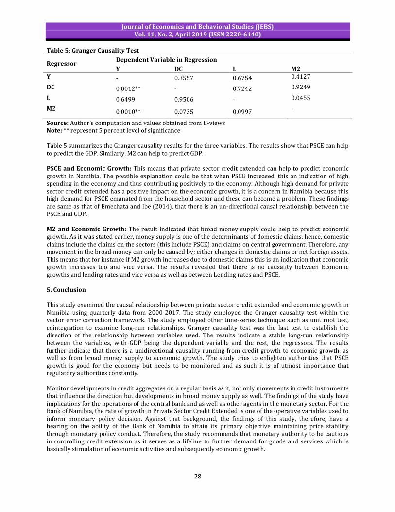
Journal of Economics and Behavioral Studies (JEBS) Vol. 11, No. 2, April 2019 (ISSN 2220-6140)
28
Table 5: Granger Causality Test
Regressor Dependent Variable in Regression
Y DC L M2 Y - 0.3557 0.6754 0.4127
DC 0.0012** - 0.7242 0.9249
L 0.6499 0.9506 - 0.0455
M2 0.0010** 0.0735 0.0997 -
Source: Author’s computation and values obtained from E-views Note: ** represent 5 percent level of significance Table 5 summarizes the Granger causality results for the three variables. The results show that PSCE can help to predict the GDP. Similarly, M2 can help to predict GDP. PSCE and Economic Growth: This means that private sector credit extended can help to predict economic growth in Namibia. The possible explanation could be that when PSCE increased, this an indication of high spending in the economy and thus contributing positively to the economy. Although high demand for private sector credit extended has a positive impact on the economic growth, it is a concern in Namibia because this high demand for PSCE emanated from the household sector and these can become a problem. These findings are same as that of Emechata and Ibe (2014), that there is an un-directional causal relationship between the PSCE and GDP. M2 and Economic Growth: The result indicated that broad money supply could help to predict economic growth. As it was stated earlier, money supply is one of the determinants of domestic claims, hence, domestic claims include the claims on the sectors (this include PSCE) and claims on central government. Therefore, any movement in the broad money can only be caused by; either changes in domestic claims or net foreign assets. This means that for instance if M2 growth increases due to domestic claims this is an indication that economic growth increases too and vice versa. The results revealed that there is no causality between Economic growths and lending rates and vice versa as well as between Lending rates and PSCE. 5. Conclusion This study examined the causal relationship between private sector credit extended and economic growth in Namibia using quarterly data from 2000-2017. The study employed the Granger causality test within the vector error correction framework. The study employed other time-series technique such as unit root test, cointegration to examine long-run relationships. Granger causality test was the last test to establish the direction of the relationship between variables used. The results indicate a stable long-run relationship between the variables, with GDP being the dependent variable and the rest, the regressors. The results further indicate that there is a unidirectional causality running from credit growth to economic growth, as well as from broad money supply to economic growth. The study tries to enlighten authorities that PSCE growth is good for the economy but needs to be monitored and as such it is of utmost importance that regulatory authorities constantly. Monitor developments in credit aggregates on a regular basis as it, not only movements in credit instruments that influence the direction but developments in broad money supply as well. The findings of the study have implications for the operations of the central bank and as well as other agents in the monetary sector. For the Bank of Namibia, the rate of growth in Private Sector Credit Extended is one of the operative variables used to inform monetary policy decision. Against that background, the findings of this study, therefore, have a bearing on the ability of the Bank of Namibia to attain its primary objective maintaining price stability through monetary policy conduct. Therefore, the study recommends that monetary authority to be cautious in controlling credit extension as it serves as a lifeline to further demand for goods and services which is basically stimulation of economic activities and subsequently economic growth.
Journal of Economics and Behavioral Studies (JEBS) Vol. 11, No. 2, April 2019 (ISSN 2220-6140)
29
References Akpansung, A. O. & Babalola, S. J. (2011). Banking Sector Credit and Economic Growth in Nigeria: An
Empirical Investigation. CBN Journal of Applied Statistics, 2(2), 52-62. Ananzeh, I. E. N. (2016). Relationship between Bank Credit and Economic Growth: Evidence from Jordan.
International Journal of Financial Research, 7(2), 53-63. Ashipala, J. & Haimbodi, N. (2003). The impact of Public Investment on Economic Growth in Namibia,
Namibia Economic Policy Research Unit Working Paper No. 88 Bank of Namibia. (2009). Annual Report. Windhoek. Bank of Namibia. (2014). Monetary Policy Stance, August 2014. Windhoek. Bank of Namibia. (2015). Annual Report. Windhoek. Belinga, T. & Doumbe, E. (2016). Causality Relationship between Bank Credit and Economic Growth: Evidence
from a Time Series Analysis on a Vector Error Correction Model in Cameroon. School of Economics, Wuhan University of Technology, China.
Central Bureau of Statistics. (2000-2007). National Accounts. Windhoek. Emecheta, B. C. & Ibe, R. C. (2014). Impact of Bank Credit on Economic Growth in Nigeria. European Journal of
Accounting Auditing and Finance Research, 2(9), 11-21. Enders, W. (2010). Applied Econometric Times Series (3rd Ed), Wiley. Gerber, M. (2009). Principles of Economics, Polytechnic of Namibia. Windhoek. Haruna, M. A., Yahya, Z. A. & Nasiru, A. (2013). Private Sector Credit and Economic Growth Nexus in Nigeria:
An Autoregressive Distributed Lag Bound Approach. Department of Economics, Usman Danfodiyo University, Sokoto.
Martynova, N. (2015). Effect of Bank Capital Requirements on Economic Growth: A Survey. De Nederlandsche Bank, Netherlands
Mishkin, F. S. (2007). The Economics of Money and Financial Markets, Pearson/Addison Wesley. Mishra, P. K., Das, K. B. & Pradhan, B. B. (2009). Credit Market Development and Economic Growth in India.
Middle Eastern Finance and Economics, 5, 92-106. Mushendami, P. (2007). Financial development and Economic growth in Namibia. Master’s thesis, University
of Namibia, Windhoek. Okafor, I. G., Chijindu, E. H. & Ugochukwu, S. (2016). Relationship between Deposit Money Bank Credit and
Economic Growth in Nigeria under a VAR G-Causality Environment. Department of Banking and Finance, Caritas University, Enugu.
Puryan, V. (2017). The Causal Relationship between Economic Growth, Banking Sector Development and Stock Market Development in Selected Middle-East and North African countries. International Journal of Economics and Financial Issues, 7(3), 575-580.
Sindano, A. (2009). The Direction of Causal Relationship between Financial Development and Economic Growth in Namibia. Master’s thesis, University of Namibia, Windhoek.
Sherbourne, R. (2010). Guide to the Namibian Economy 2010, Institute for Public Policy Research, Windhoek, Namibia.
Spencer, H. M. (1977). Contemporary Macroeconomics (3rd Ed), Worth Publishers, New York. Yakubu, Z. & Affoi, A. Y. (2013). An Analysis of Commercial Banks’ Credit on Economic Growth in Nigeria
Department of Economics, Kaduna State College of Education, Gidan Waya, Kafanchan, Kadun State, Nigeria.

Journal of Economics and Behavioral Studies (JEBS) Vol. 11, No. 2, April 2019 (ISSN 2220-6140)
30
Significant Factors Influencing Quality Assurance Practices in Small and Medium-Sized Construction Projects in South Africa
Kgashane Stephen Nyakala1, Thinandavha Thomas Munyai1, Jan-Harm Pretorius2, Andre Vermeulen2
1Tshwane University of Technology, South Africa 2University of Johannesburg, South Africa
[email protected] Abstract: Although implementing quality assurance (QA) processes in construction play an important role in the South African economy has been acknowledged. However, constructions SMEs are faced with difficulties in improving rural road infrastructure and high-quality roads. Additionally, past research has failed to reach consensus on the construction process and socioeconomic settings in previously disadvantaged areas in South Africa, including the factors influencing negatively the performance of such factors. This research examines what factors facilitate or inhibit the success of construction SMEs and what actions can be taken to being distressed construction SMEs under control. The study adopted a quantitative research approach in which a three-section questionnaire was administered to 160 purposively chosen road- building experts in a South African construction SMEs. The questionnaire was structured into three parts, which sought the participants’ profile, identified the quality assurance practices (QAPs) incorporated in the construction SMEs’ road building programmes, and identified the factors that negatively influence the implementation of QA processes. Data was analysed using the Statistical Package for the Social Sciences (SPSS) version 22. Furthermore, to determine the reliability of the various constructs, mean scores, descriptive statistics and standard deviations were obtained. The empirical findings established eight QAPs that were reliable and valid for implementation processes that can control or minimise their causes of poor quality in projects undertaken by construction SMEs, level of skill acquisition; project planning and control techniques; project construction design; process implementation and process improvement; financial management; organisational structures; involvement of people; and quality standards and measurements. The eight factors attained high Cronbach Alpha values above the recommended 0.70 which indicates high internal consistencies among the sub-scales. Findings from this study should be useful to managers in similar environments may use the results of this study as either diagnostic tools or as a reference benchmark for strategic interventions in solving construction projects related problems. Furthermore, the researchers also recommend that these practices are for quality assurance in construction projects undertaken by SMEs in South Africa. Keywords: South Africa, SME construction projects, quality assurance practice, road construction
1. Introduction The construction industry is considered a key industry in any economy. The construction sector in Southern Africa itself is a challenging field of work because there are many multifaceted responsibilities and operational procedures (Mofokeng & Thwala, 2012: 712; Windapo & Cattel, 2013; George, 2016:24). According to the annual report on South African SME construction projects, there existed 30.1 % to 39.4 % inefficiency, poor quality of rural road building and lack of construction process planning amongst SMEs contractors (Statistics South Africa, 2017). In addition, improper implementation of rural road construction projects causes considerable problems for contractors (Vermeulen et al., 2018). Construction organisations display distinctive characteristics, combined with the varying demands of the industry’s stakeholders, which includes uniting varied investors, clients, consulting professions and contractual engagements (Badu & Owusu-Manu, 2011:271; Construction Industry Development Board (CIDB), 2012). Construction SMEs can be described as those SMEs which work on construction projects, comprising some components of the design and control of construction works as well as the quantity of building materials, tools, equipment, plant, transport and other services (Rumane, 2011). The South African local government is obliged to render basic services for the people, with a special focus on the provision of roads in the local communities they serve. Adequate road contributes immensely to the economic growth, development and redistribution (Statistics South Africa, 2017). Roads network infrastructure delivery should ensure and provide good outcomes for the public (Nyakala et al., 2017:636). Total quality management research in the construction process has
Journal of Economics and Behavioral Studies (JEBS) Vol. 11, No. 2, April 2019 (ISSN 2220-6140)
31
revealed that improving staff performance, customer satisfaction and confidence in the organisation’s products/services are beneficial to all construction and business organisations (Arditi & Gunaydin, 1997). Understanding the relationship between process quality and product quality could consequently be useful in cultivating the QAPs that can reduce poor quality and cost overruns in construction projects. It is imperative to discover this relationship, mainly because of the great impact of the construction sector on the economy of a country. Fang and Wu (2013:139) note that good transport infrastructure has a positive influence mostly on the life of the rural people, and supports the establishment of effective co-ordinating constructions throughout government to promote efficiency in road service delivery. To provide quality service delivery, all employees in a road network infrastructure, therefore, need to understand project management techniques and tools, (Basu, 2004). The specific question to be answered here is: “What aspects expedite the practice of QA processes in road construction projects? The present paper follows preceding efforts to understand the processes of improving the quality of the construction projects (Ahadzie et al., 2007:806). There is also much agreement concerning the benefits expected from effective contractor development, encompassing global attractiveness, sustainable industry growth, good environmental management and socio-economic development of the developing countries (Van Wyk, 2003). It is thus important that QA processes should be practiced in the South African construction industry. Seemingly, lessons learned have possibilities to enhance the image of the QA process implementation (Vermeulen et al., 2018:1). The aims of this paper are to examine key factors that influence QAPs in construction SMEs and uncover the collective working practices that can control or minimise causation characteristics. The result is not only useful to participants in the QA processes implementation within the construction industry but also to societies in other countries, and the rest of the world. In order to understand the implementation process of QAPs in construction SMEs, it is important to introduce the present theory on the quality management concepts included in this study. The current theory focuses on the overall concepts on the quality management in the construction project and project management; structures and QA involves establishing project related policies, procedures, standards, training, guidelines and systems necessary to produce quality. The improvement and prioritisation of rural roads networks play a vital role in developing countries to improve the socioeconomic conditions experienced by societies. However, a wide range of challenges is encountered by SMEs in the construction industry when dealing with construction projects, and as a result, poor quality and poor performance of work is prevalent. South Africa is mostly characterised by the failure of small businesses’ entrepreneurial capacity, which is largely characterised by low levels of entrepreneurial education (Mofokeng & Thwala, 2012). The reason for this is that there is incomplete accessibility of road network infrastructure and high volume roads in rural connectivity, crisis management, and liveability (Fang & Wu, 2013; Nyakala et al., 2017:640). It is against this background that this study was introduced to examine the factors that influence QAPs in construction projects. In order to achieve the aim of this study, two objectives were set out: to examine the QAPs incorporated in the rural road infrastructure of construction SMEs, and to determine the factors that positively influence the practice of construction SMEs. Identifying such factors will assist management to the success of QAPs are put in place to deal with such matters, which, in the long term, will cause a huge decrease in misfortunes that occur on construction SMEs. Quality Assurance in SMEs: The literature review identified a number of quality assurance in SMEs designed to maximize employee performance in facilitating a business’s strategic objectives (Basu, 2004; Freeman-Bell & Balkwill, 1996; Aziz & Abdel-Hakam, 2016; Panuwatwanich & Nguyen, 2017). Various researchers on quality management approaches have agreed that unless SME contractors play an active role and take the lead to improve productivity management in the civil construction industry, efforts and gains made by individuals and departments will be short-lived (Arditi & Gunaydin, 1997; Basu, 2004; Bierman, et al., 2013). As Mofokeng and Thwala (2012:713) mention, leadership can influence project success by establishing an environment, where project teams contribute towards success. In South Africa, project managers and project consultants are responsible for the overall construction success related to delivering infrastructure projects within the approved costs and time as well as the necessary quality and supervision. The above proposed broad view of project success also stresses the necessity for a joint performance assessment between project participants. As indicated earlier, quality cannot be seen by SMEs as an expensive process, an expensive

Journal of Economics and Behavioral Studies (JEBS) Vol. 11, No. 2, April 2019 (ISSN 2220-6140)
32
product, or time-consuming but can improve their competitive capabilities in the marketplace (Kruger et al., 2014). Level of Skill Acquisition Process: Mofokeng & Thwala (2012:722) postulated that, the construction organisations needed to spearhead the capacitation of employees through the process of skill acquisition and facilitating employees’ new skills. Aziz & Gunaydin (1997) notes that opportunities for skills development in the construction industry had grown significantly and the main drivers were growth of businesses and infrastructures, environmental pressures and sustainability as well as management commitment. The literature review identified a number of quality management procedures in organisations designed to maximize employee performance in facilitating a business’s strategic objectives (Basu, 2004; Freeman-Bell & Balkwill, 1996; Aziz & Abdel-Hakam, 2016; Panuwatwanich & Nguyen, 2017). Mahmood et al. (2010) established that, for any built environment project to improve its competitive abilities in the construction industry, it should be able to determine the cost of poor quality and its impact on productivity and profitability. The success of construction projects is grounded on the individual competencies of site managers or project managers responsible for the execution process (Fotopoulos & Psomas, 2009). Vermeulen et al. (2018:2) have clarified the main contributors of South African construction project participants as the designer or architect, the client, the project/construction manager and the contractors, which are then extended with many sub-teams with their own leaders who perform different functions. Project Planning and Control Techniques: Successful implementation of QA developments necessitate actual planning and control practices, operations and review as well as stakeholder approval for business project activities (Nyakala et al., 2017:650). To effectively implement their QAPs, construction SMEs must meet their approved quality objectives and detailed requirements. Windapo & Cattel (2013) state that for the successful execution of a project, effective planning is essential. A project manager holds the same responsibilities facil itates a formal system for record keeping, and provide work breakdown detail to all stakeholders (CIDB, 2012). Construction project management should include the design and execution of the infrastructure, the environmental impact of the job, the successful scheduling, budgeting, accessibility and delivery of building resources, inconvenience to the public affected by construction delays and bidding (Arditi & Gunaydin, 1997; Rumane, 2011; Tshivhase & Worku, 2012:62). Formal techniques of project management must be utilised by SME road contractors to enable citizens to have quality road networks and access to public services such as education, health facilities and the movement of labour between workplaces (Vermeulen et al., 2018:2). In addition to that, quality controls are required to prevent the deterioration of maintenance backlogs, and focus the efforts that the project manager has to spend on the daily control of the numerous activities of the project (Thorpe et al., 1996; Panuwatwanich & Nguyen, 2017). Project Construction Design: The context of project construction design within construction SMEs raised the question as to how senior project managers could adopt measurement tool in relation to QA processes and scope of work reporting on mistakes by the project team. Kerzner (2013) who state that the chief engineer is responsible for organizing technical personnel optimization of construction scheme, improving the technical measures as well as providing technical support for the effective cost control also supports this view. According to Kam and Hamid (2014:603), an example of an industry that heavily adopted the technology was manufacturing. As identified by computerized project management has been introduced in construction organisations such as Microsoft Project and Oracle Primavera further state that technical inspection of the construction progress with a high level of reliability was applicable in the early stages of a construction project. One major practical issue that has dominated the road construction projects for many years concerns the unpredictability in project construction designs creating complications when implementing processes of QA to the industry. Process Implementation: The significance of applying proper management in dealing with the processes of QA in construction needed to be highlighted by the senior management team. The study analysed the project management tools that needed to be practiced in the local construction industry to enhance effective road construction projects. A recent study conducted by Aziz et al. (2016) found that having more experienced and capable construction managers, a s wel l a s s k i l l ed l a bo ur ers , helped to enable the industry to develop at a faster rate either nationally or internationally. In the study, it was shown that the proper process implementation of quality assurance system helped organisations to better organise

Journal of Economics and Behavioral Studies (JEBS) Vol. 11, No. 2, April 2019 (ISSN 2220-6140)
33
and synchronize their operations by documenting their procedures, clearly defining responsibilities and tasks among employees and subdivisions (Gotzamani & Tsiotras, 2001). Project management also includes practical implementation (Olawale & Sun, 2015), and it is widely accepted and well- documented that implementing QA processes presents a good opportunity for organisations that want to respond to the challenge. In the South African local government, such knowledge gaps are critically confronted by a lack of communication technologies. The minority of participants indicated that the local authority as very good rated 10.6 per cent of the SMEs projects. Financial Management Skills: Financial management is a key factor influencing construction industry. The timely completion of road construction projects is considered one of the key factors referring to the project achievement as well as the quality and the safety (Aziz et al., 2016). In line with this, a cost-effective policy, competence and profitability are the main determinants of construction process planning, covering activities needed to deliver quality in work to meet the project requirements (Mahmood et al., 2010). Costs of restructuring the process must be controlled to eradicate the causes of poor quality and related preventive activities. The encompasses, for example, preparation, monitoring and analysis, project review, and quality improvement programs (Nyakala et al., 2017:650). Quality training and project control systems are essential for innovation and for technology advancement, and a standard of living improvement (Obare et al., 2016). The implementation of project control systems perpetuates them as engines through which the growth objectives of developing countries can be achieved (Ahadzie et al., 2007). Quality Standards in the Construction Project: Quality standard scope signifies organisational performance through construction project management, quality policy, organisational structures and successful implementation of quality working practices by construction SMEs in the country (Vermeulen et al., 2018:3). The success of any construction organisation depends on how corporate strategies adopt continuous quality improvement practices (Kerzner, 2013). This will be supplemented in practical terms by implementing total quality strategies and empower employees in the construction project to identify opportunities and develop them more efficiently (Gardiner, 2005). During building operations, there must be quality control to ensure that the roads are constructed to expectations (Honnakker et al., 2010:954). Quality control verifies that processes are performed in a satisfactory manner (Kruger et al., 2014). Quality product procedures, product reliability, standards and dimensions are essential. These allow the contractor to evaluate and assess project processes against applicable standards, quality management tools and techniques, total quality management (TQM), cause-and-effect diagrams, policies and procedures (Gardiner, 2005). Organisational Structure and Improvement Programs in SMEs: SME construction organisations are less able to deal with ‘disclosures’ in the global economy and as a result are mostly vulnerable. SME road construction projects need to be managed and controlled to allow goal setting for reconstruction, growth and improvement in the construction industry (Vermeulen et al., 2018). These gaps further include inadequate connectivity and mobility to reach out and open up new opportunities and improper physical infrastructure and economic developments. Enhancing competitiveness in the construction industry is measured to be a strategic prospect if it seems to be improving quality developments and incorporating engineering management principles and practices (Freeman-Bell & Balkwill, 1996). Contractor development tools that meet challenges of globalisation are nowadays considered as techniques that frequently maintain the management of construction projects, multitudes of data, and tight deadlines that are characteristic of numerous industries and their extremely competitive settings (Badu & Owusu-Manu, 2011). Construction SMEs need computerised systems that follow the value chain in construction project delivery (Arditi & Gunaydin, 1997). This supports the notion that quality must be built-in during design and are achieved through communication, development and improvement (Bierman et al., 2013; Olawale & Sun, 2015). Organisational structure should put in place to support people and organisations in their pursuit of better quality. Such measures comprise an extensive variability of tools to plan work activities, gather data, analyse outcomes, monitor progress and solve problems (Bierman et al., 2013:44). Fotopoulos & Psomas (2009) stated that techniques need to used and focus on improving quality activities in the construction industry. Basu (2004) suggested the statistical techniques of experimental design to optimise process sceneries to decrease scrap or increase yield. Project managers responsible for this frequently look at process

Journal of Economics and Behavioral Studies (JEBS) Vol. 11, No. 2, April 2019 (ISSN 2220-6140)
34
implementation, process optimisation, and practical implementation, future systems of the process, process expertise and process design (Kerzner, 2013). People Involvement: Top management can influence project success by creating an environment where project teams contribute towards success (Van Wyk, 2003) argue that an organisation’s success depends increasingly on having opportunities to acquire, meet, collaboration and practicing new skills. This can evidently influence project success. According to Badu & Owusu-Manu (2011:270), the critical success factor lies in the construction organisations’ real commitment to quality improvement and their true target of certification, which finally commands the way and depth to which the standards are implemented. Employee involvement and empowerment has been identified as influential in planning of on-site construction process and organisational performance (Windapo & Cattel, 2013). It is consequently important for workforces to be involved and empowered in construction planning process by, for example, being able to prepare and meet project teams, use of equipment and the skills and knowledge required to do work effectively (Thorpe et al., 1996; Rumane, 2011). Employees should further be able to share resources, schedule project activities and respond to memos and emails to construction senior management (Aigbavboa & Thwala, 2014:773). It is also important for SME contractors to be committed and involved in the processes of QA implementation at SME led project level. Factors that Influence Quality Assurance Practices of Construction Projects: A study by Obare et al. (2016:420) point out that the quality cost model evaluation of quality management practices customer focus teamwork employee empowerment education and continuous improvement influenced project success in addition, Fotopoulos & Psomas (2009) also asserted that performing check-up, analysis, and corrective actions seemed to obtain customer’s satisfaction. Martins & Lewis (2014) indicated that an effective communication system between project team leaders and management is crucial to the success of construction projects. Windapo & Cattel (2013), postulate that this is generally influenced by alignment of management commitment and subordinate actions. Karna & Junnonen (2017:154) indicated that effective designers’ performance evaluation in construction projects positively influence the success of a project. Jarkas & Younes (2014:61) stipulated that, in situations where management commitment is to be ineffective, these should be revised, or new control actions be implemented, thus enabling continuous improvement in construction projects. In reviewing literature, a number of studies have criticized the systems of managing quality during construction process (Arditi & Gunaydin, 1997). It has been recommended that the failure of many road construction projects in South Africa may partially be ascribed to t h e poor quality of road constructed by SME contractors in the country (Dangalazana & Newadi, 2005; Statistics South Africa, 2017). Vermeulen et al. (2018) opined that developing key success criteria for rural development initiatives provides a positive contribution to projects. 2. Methodology The purpose of this research was to determine the factors that influence QAPs that can be implemented for construction SMEs to facilitate or inhibit their projects, in order to achieve project success. A quantitative research design was used, in which the use of structured questionnaire surveys enables researchers to generalise their findings from a sample of population. In the questionnaire, seven QAPs (constructs), consisting of 35 measures, were extracted and set as the variables of quality assurances practices SMEs should follow (Pallant, 2013:192). Exploratory Factor Analysis (EFA) was utilised to assess these measured variables in relation to their validity and reliability. Likert scale was utilised, whereby each participant indicated the degree to which they agreed or disagreed with its contents hence emphasising the significance of choosing the desired response (Leedy & Ormrod, 2014). According to Pallant (2013:192), EFA can be seen as a type of technique that analyses the characteristics (unidimensionality) of each of the defined QAPs (original variables), in order to reduce it to a common score (smaller number of factors) by examining relationships among these quantitative factors. Various data-analysis strategies are available; Kaiser-Meyer-Olkin (KMO) Bartlett’s Test of Sphericity was used to determine whether the correlation matrix is an identity matrix stating if the factor model is inappropriate (Tabachnick & Fidell, 2007). Sampling Method and Response Rate: Construction S M E s based local municipalities in Mopani District Municipality constituted the study’s population. A total of 160 questionnaires were returned, representing a

Journal of Economics and Behavioral Studies (JEBS) Vol. 11, No. 2, April 2019 (ISSN 2220-6140)
35
64% response rate of the 250 questionnaires distributed. The local office of Road and Public Works from the District were approached to assist with the compilation of the list. After distributing numbers to form sampling frames, the researcher then used a sample random sampling method to randomly select five projects from each of the five sampling frames. This resulted in the selection of 10 projects (from the initial five projects) from each of the Limpopo Local Municipalities of Mopani District Municipality. The sample of n=160 participants completed the questionnaire. The sample size table Krejcie & Morgan (1970:608) recommends a sample size for a population of 500 of 217. This recommendation validates the sample size of 250 as efficient for the population of 160. The people contacted for the questionnaires are in the know of the past and current SME projects in the South African construction industry. They were authorized by their organizations to participate in the study as they were involved in rural road projects for their respective organisations. However, pseudo numbers and names were used to classify the participants for analysis of data purposes. Data Collection: Questionnaires were distributed to the prospective respondents who worked on the road construction projects in the local municipalities of Limpopo Province in South Africa, from November 2016 to August 2017. The measuring instrument used in this study included a structured questionnaire survey using Likert-ranking scales as well as open-ended questions to generate qualitative data. Both questionnaires were pre-tested in this study. Questionnaires that are completed by respondents themselves are one of the main instruments for collecting data using a social survey design describe a questionnaire as a method that can be used without direct personal contact with respondents, as these are questionnaires to be completed by respondents. The questionnaires were administered and comprised of two sections. Section A was the biographic profile of the targeted population, namely, age, the highest educational level obtained, number of years’ experience in the business and type of ownership in the business. Section B focused on the project characterisation relating to performance variables, namely, road quality construction projects, QAPs, quality management systems and procedures, implementation process, SME contractors as well as CIDB educational needs. In such a situation, anonymity and confidentiality were guaranteed participants were not requested to provide personal details such as names, identity numbers and their physical address. Section B firstly required that respondents indicated the “level of implementation” achieved at their business for each process and then they rated the importance of each process in achieving a high-quality road construction project. It also demonstrates the design of the section B questionnaire performed a gap analysis between what contractors perceived as a level of implementation versus attaining high-quality standards. This enabled the study to achieve its objectives as well as determining disparities between quality of implementation factor-items and rating of importance factor-items. Section B’s criteria were derived as an analytic tool from the factors influencing positive impact of QAPs and then identified and compiled a set of 35 measurable items. It can also be stated that these items were clustered according to the eight (8) Relevance Factors or aspects. Phase B was derived from the review of literature, preliminary study, and, as such, was comprised of a Likert scale development questionnaire. Criteria and critical success aspects of QA processes related to road construction projects. In enquiring questions, researchers have two choices, namely, the questionnaire items may be closed-ended, open-ended, or both (Teddlie & Tashakkori, 2009:232). It can also be stated that these items were clustered according to the eight (8) Relevance Factors or aspects. Analysis and Interpretation of the Data: The Statistical Package for the Social Sciences (SPSS) version 22 was used to conduct descriptive, statistical analysis of the data computing the frequencies, mean scores and standard deviations. SPSS was further utilised to determine the feasibility of conducting a factor analysis of the QAPs survey results relating to the QA processes implementation in the construction project delivery. Cronbach’s alpha coefficient indicates the average correlation among all the items that make up the scale, in order to determine the reliability of the measuring instrument (Kaiser, 1974). Likewise, exploratory factor analysis (EFA) was used to determine the unidimensionality of the QA road construction processes and their reliability. Reliability was tested using Cronbach’s Alpha with a cut-off value of 0.70 (Hair, Black, Anderson & Tatham, 2014). SPSS indicates that Kaiser-Meyer-Olkin (KMO) Bartlett’s Test of Sphericity was used to determine whether the correlation matrix is an identity matrix stating if the factor model is inappropriate (Tabachnick & Fidell, 2007). Thus, it measures the index of the appropriateness of factor analysis for overall statistics including each
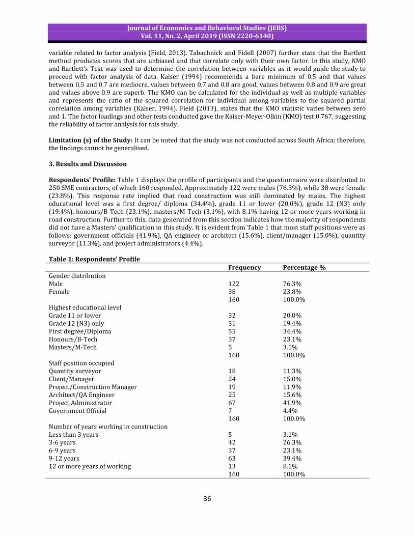
Journal of Economics and Behavioral Studies (JEBS) Vol. 11, No. 2, April 2019 (ISSN 2220-6140)
36
variable related to factor analysis (Field, 2013). Tabachnick and Fidell (2007) further state that the Bartlett method produces scores that are unbiased and that correlate only with their own factor. In this study, KMO and Bartlett’s Test was used to determine the correlation between variables as it would guide the study to proceed with factor analysis of data. Kaiser (1994) recommends a bare minimum of 0.5 and that values between 0.5 and 0.7 are mediocre, values between 0.7 and 0.8 are good, values between 0.8 and 0.9 are great and values above 0.9 are superb. The KMO can be calculated for the individual as well as multiple variables and represents the ratio of the squared correlation for individual among variables to the squared partial correlation among variables (Kaiser, 1994). Field (2013), states that the KMO statistic varies between zero and 1. The factor loadings and other tests conducted gave the Kaiser-Meyer-Olkin (KMO) test 0.767, suggesting the reliability of factor analysis for this study. Limitation (s) of the Study: It can be noted that the study was not conducted across South Africa; therefore, the findings cannot be generalised. 3. Results and Discussion Respondents’ Profile: Table 1 displays the profile of participants and the questionnaire were distributed to 250 SME contractors, of which 160 responded. Approximately 122 were males (76.3%), while 38 were female (23.8%). This response rate implied that road construction was still dominated by males. The highest educational level was a first degree/ diploma (34.4%), grade 11 or lower (20.0%), grade 12 (N3) only (19.4%), honours/B-Tech (23.1%), masters/M-Tech (3.1%), with 8.1% having 12 or more years working in road construction. Further to this, data generated from this section indicates how the majority of respondents did not have a Masters’ qualification in this study. It is evident from Table 1 that most staff positions were as follows: government officials (41.9%), QA engineer or architect (15.6%), client/manager (15.0%), quantity surveyor (11.3%), and project administrators (4.4%). Table 1: Respondents’ Profile Frequency Percentage % Gender distribution Male 122 76.3% Female 38 23.8% 160 100.0% Highest educational level Grade 11 or lower 32 20.0% Grade 12 (N3) only 31 19.4% First degree/Diploma 55 34.4% Honours/B-Tech 37 23.1% Masters/M-Tech 5 3.1% 160 100.0% Staff position occupied Quantity surveyor 18 11.3% Client/Manager 24 15.0% Project/Construction Manager 19 11.9% Architect/QA Engineer 25 15.6% Project Administrator 67 41.9% Government Official 7 4.4% 160 100.0% Number of years working in construction Less than 3 years 5 3.1% 3-6 years 42 26.3% 6-9 years 37 23.1% 9-12 years 63 39.4% 12 or more years of working 13 8.1% 160 100.0%
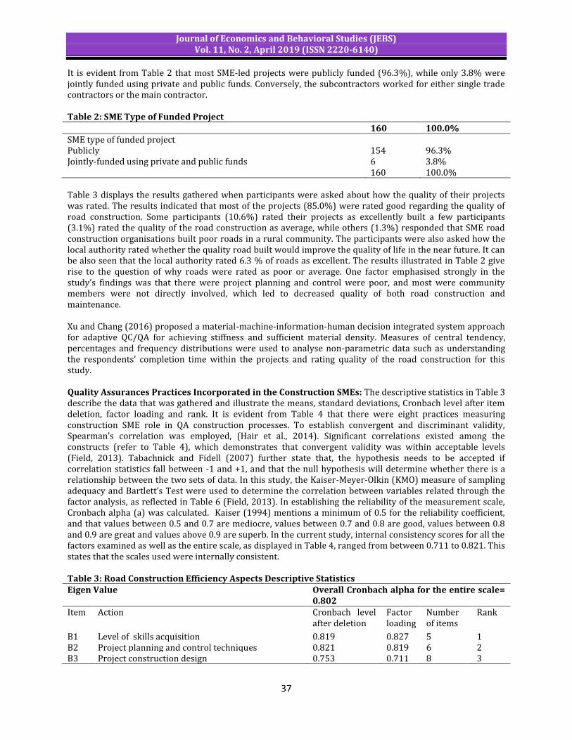
Journal of Economics and Behavioral Studies (JEBS) Vol. 11, No. 2, April 2019 (ISSN 2220-6140)
37
It is evident from Table 2 that most SME-led projects were publicly funded (96.3%), while only 3.8% were jointly funded using private and public funds. Conversely, the subcontractors worked for either single trade contractors or the main contractor. Table 2: SME Type of Funded Project 160 100.0% SME type of funded project Publicly 154 96.3% Jointly-funded using private and public funds 6 3.8% 160 100.0% Table 3 displays the results gathered when participants were asked about how the quality of their projects was rated. The results indicated that most of the projects (85.0%) were rated good regarding the quality of road construction. Some participants (10.6%) rated their projects as excellently built a few participants (3.1%) rated the quality of the road construction as average, while others (1.3%) responded that SME road construction organisations built poor roads in a rural community. The participants were also asked how the local authority rated whether the quality road built would improve the quality of life in the near future. It can be also seen that the local authority rated 6.3 % of roads as excellent. The results illustrated in Table 2 give rise to the question of why roads were rated as poor or average. One factor emphasised strongly in the study’s findings was that there were project planning and control were poor, and most were community members were not directly involved, which led to decreased quality of both road construction and maintenance. Xu and Chang (2016) proposed a material-machine-information-human decision integrated system approach for adaptive QC/QA for achieving stiffness and sufficient material density. Measures of central tendency, percentages and frequency distributions were used to analyse non-parametric data such as understanding the respondents’ completion time within the projects and rating quality of the road construction for this study. Quality Assurances Practices Incorporated in the Construction SMEs: The descriptive statistics in Table 3 describe the data that was gathered and illustrate the means, standard deviations, Cronbach level after item deletion, factor loading and rank. It is evident from Table 4 that there were eight practices measuring construction SME role in QA construction processes. To establish convergent and discriminant validity, Spearman’s correlation was employed, (Hair et al., 2014). Significant correlations existed among the constructs (refer to Table 4), which demonstrates that convergent validity was within acceptable levels (Field, 2013). Tabachnick and Fidell (2007) further state that, the hypothesis needs to be accepted if correlation statistics fall between -1 and +1, and that the null hypothesis will determine whether there is a relationship between the two sets of data. In this study, the Kaiser-Meyer-Olkin (KMO) measure of sampling adequacy and Bartlett’s Test were used to determine the correlation between variables related through the factor analysis, as reflected in Table 6 (Field, 2013). In establishing the reliability of the measurement scale, Cronbach alpha (a) was calculated. Kaiser (1994) mentions a minimum of 0.5 for the reliability coefficient, and that values between 0.5 and 0.7 are mediocre, values between 0.7 and 0.8 are good, values between 0.8 and 0.9 are great and values above 0.9 are superb. In the current study, internal consistency scores for all the factors examined as well as the entire scale, as displayed in Table 4, ranged from between 0.711 to 0.821. This states that the scales used were internally consistent. Table 3: Road Construction Efficiency Aspects Descriptive Statistics Eigen Value
Overall Cronbach alpha for the entire scale= 0.802
Item Action Cronbach level after deletion
Factor loading
Number of items
Rank
B1 Level of skills acquisition 0.819 0.827 5 1 B2 Project planning and control techniques 0.821 0.819 6 2 B3 Project construction design 0.753 0.711 8 3
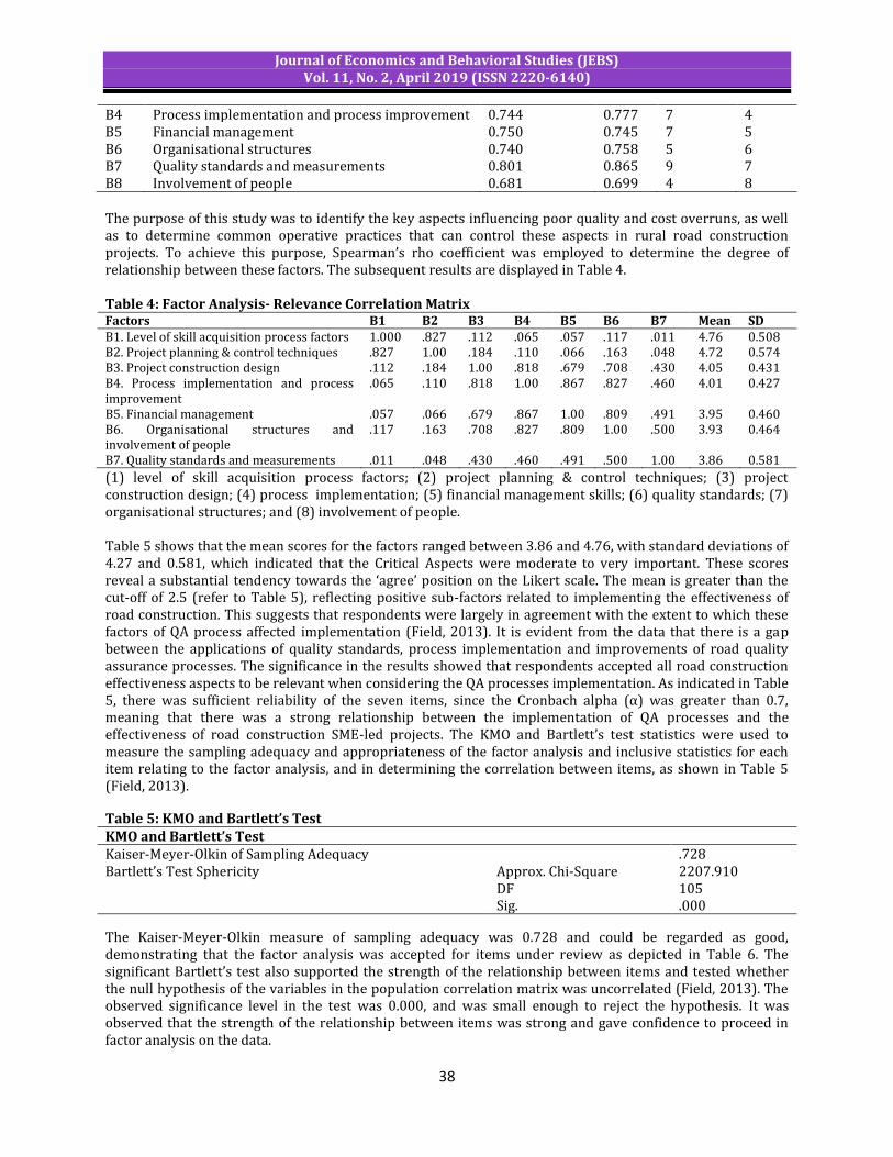
Journal of Economics and Behavioral Studies (JEBS) Vol. 11, No. 2, April 2019 (ISSN 2220-6140)
38
B4 Process implementation and process improvement 0.744 0.777 7 4 B5 Financial management 0.750 0.745 7 5 B6 Organisational structures 0.740 0.758 5 6 B7 Quality standards and measurements 0.801 0.865 9 7 B8 Involvement of people 0.681 0.699 4 8 The purpose of this study was to identify the key aspects influencing poor quality and cost overruns, as well as to determine common operative practices that can control these aspects in rural road construction projects. To achieve this purpose, Spearman’s rho coefficient was employed to determine the degree of relationship between these factors. The subsequent results are displayed in Table 4. Table 4: Factor Analysis- Relevance Correlation Matrix Factors B1 B2 B3 B4 B5 B6 B7 Mean SD B1. Level of skill acquisition process factors 1.000 .827 .112 .065 .057 .117 .011 4.76 0.508 B2. Project planning & control techniques .827 1.00 .184 .110 .066 .163 .048 4.72 0.574 B3. Project construction design .112 .184 1.00 .818 .679 .708 .430 4.05 0.431 B4. Process implementation and process improvement
.065 .110 .818 1.00 .867 .827 .460 4.01 0.427
B5. Financial management .057 .066 .679 .867 1.00 .809 .491 3.95 0.460 B6. Organisational structures and involvement of people
.117 .163 .708 .827 .809 1.00 .500 3.93 0.464
B7. Quality standards and measurements .011 .048 .430 .460 .491 .500 1.00 3.86 0.581
(1) level of skill acquisition process factors; (2) project planning & control techniques; (3) project construction design; (4) process implementation; (5) financial management skills; (6) quality standards; (7) organisational structures; and (8) involvement of people. Table 5 shows that the mean scores for the factors ranged between 3.86 and 4.76, with standard deviations of 4.27 and 0.581, which indicated that the Critical Aspects were moderate to very important. These scores reveal a substantial tendency towards the ‘agree’ position on the Likert scale. The mean is greater than the cut-off of 2.5 (refer to Table 5), reflecting positive sub-factors related to implementing the effectiveness of road construction. This suggests that respondents were largely in agreement with the extent to which these factors of QA process affected implementation (Field, 2013). It is evident from the data that there is a gap between the applications of quality standards, process implementation and improvements of road quality assurance processes. The significance in the results showed that respondents accepted all road construction effectiveness aspects to be relevant when considering the QA processes implementation. As indicated in Table 5, there was sufficient reliability of the seven items, since the Cronbach alpha (α) was greater than 0.7, meaning that there was a strong relationship between the implementation of QA processes and the effectiveness of road construction SME-led projects. The KMO and Bartlett’s test statistics were used to measure the sampling adequacy and appropriateness of the factor analysis and inclusive statistics for each item relating to the factor analysis, and in determining the correlation between items, as shown in Table 5 (Field, 2013).
Table 5: KMO and Bartlett’s Test KMO and Bartlett’s Test Kaiser-Meyer-Olkin of Sampling Adequacy .728 Bartlett’s Test Sphericity Approx. Chi-Square 2207.910
DF 105 Sig. .000
The Kaiser-Meyer-Olkin measure of sampling adequacy was 0.728 and could be regarded as good, demonstrating that the factor analysis was accepted for items under review as depicted in Table 6. The significant Bartlett’s test also supported the strength of the relationship between items and tested whether the null hypothesis of the variables in the population correlation matrix was uncorrelated (Field, 2013). The observed significance level in the test was 0.000, and was small enough to reject the hypothesis. It was observed that the strength of the relationship between items was strong and gave confidence to proceed in factor analysis on the data.
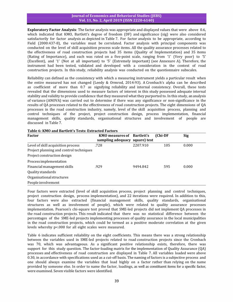
Journal of Economics and Behavioral Studies (JEBS) Vol. 11, No. 2, April 2019 (ISSN 2220-6140)
39
Exploratory Factor Analysis: The factor analysis was appropriate and displayed values that were above 0.6, which indicated that KMO, Bartlett’s degree of freedom (DF) and significance (sig) were also considered satisfactorily for factor analysis as depicted in Table 7. For factor analysis to be appropriate, according to Field (2000:437-8), the variables must be correlated. Factor analysis with principal components was conducted on the level of skill acquisition process scale items. All the quality assurance processes related to the effectiveness of road construction projects had 35 items (Quality of Implementation) and 35 items (Rating of Importance), and each was rated on a five-point scale, ranging from ‘1’ (Very poor) to ‘5’ (Excellent), and ‘1’ (Not at all important) to ‘5’ (Extremely important) (see Annexure A). Therefore, the instrument had been tested, validated and developed with a consideration in the context of road construction projects. In this study, reliability analysis was conducted on the questionnaire subscales.
Reliability can defined as the consistency with which a measuring instrument yields a particular result when the entire measured has not changed (Leedy & Ormrod, 2014:93). A Cronbach’s alpha can be described as coefficient of more than 0.7 as signifying reliability and internal consistency. Overall, these tests revealed that the dimensions used to measure factors of interest in this study possessed adequate internal stability and validity to provide confidence that they measured what they purported to. In this study, an analysis of variance (ANOVA) was carried out to determine if there was any significance or non-significance in the results of QA processes related to the effectiveness of road construction projects. The eight dimensions of QA processes in the road construction industry, namely, level of the skill acquisition process, planning and control techniques of the project, project construction design, process implementation, financial management skills, quality standards, organisational structures and involvement of people are discussed in Table 7.
Table 6: KMO and Bartlett’s Tests: Extracted Factors Factor KMO measures of
sampling adequacy Bartlett’s (Chi-square) test
DF Sig
Level of skill acquisition process .728 2207.910 105 0.000
Project planning and control techniques
Project construction design
Process implementation
Financial management skills .929 9494.842 595 0.000
Quality standards
Organisational structures
People involvement
Four factors were extracted (level of skill acquisition process, project planning and control techniques, project construction design, process implementation), and 22 iterations were required. In addition to this, four factors were also extracted (financial management skills, quality standards, organisational structures as well as involvement of people), which were related to quality assurance processes implementation. Pearson’s chi-square test proved that SME-led projects did not implement QA processes in the road construction projects. This result indicated that there was no statistical difference between the percentages of the SME-led projects implementing processes of quality assurance in the local municipalities in the road construction projects, which could be termed as a positive moderate correlation at the given levels whereby p<.000 for all eight scales were measured.
Table 6 indicates sufficient reliability on the eight coefficients. This means there was a strong relationship between the variables used in SME-led projects related to road construction projects since the Cronbach was 70, which was advantageous. As a significant positive relationship exists, therefore, there was support for this study question. The factor-loading matrix for the implementation of Quality Assurance (QA) processes and effectiveness of road construction are displayed in Table 7. All variables loaded were above 0.30, in accordance with specifications used as a cut-off basis. The naming of factors is a subjective process and one should always examine the variables that load highly on a factor rather than relying on the name provided by someone else. In order to name the factor, loadings, as well as constituent items for a specific factor, were examined. Seven visible factors were identified.
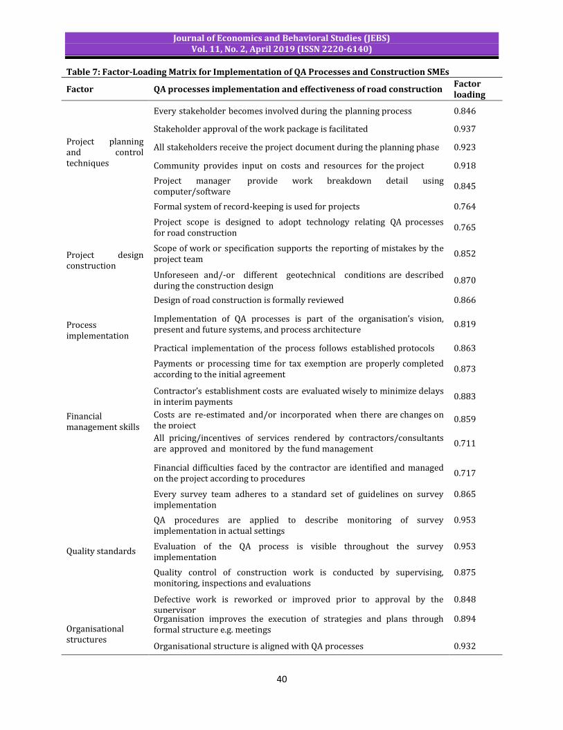
Journal of Economics and Behavioral Studies (JEBS) Vol. 11, No. 2, April 2019 (ISSN 2220-6140)
40
Table 7: Factor-Loading Matrix for Implementation of QA Processes and Construction SMEs
Factor QA processes implementation and effectiveness of road construction Factor loading
Project planning and control techniques
Every stakeholder becomes involved during the planning process 0.846
Stakeholder approval of the work package is facilitated 0.937
All stakeholders receive the project document during the planning phase 0.923
Community provides input on costs and resources for the project 0.918
Project manager provide work breakdown detail using computer/software
0.845
Formal system of record-keeping is used for projects 0.764
Project design construction
Project scope is designed to adopt technology relating QA processes for road construction
0.765
Scope of work or specification supports the reporting of mistakes by the project team
0.852
Unforeseen and/-or different geotechnical conditions are described during the construction design
0.870
Design of road construction is formally reviewed 0.866
Process implementation
Implementation of QA processes is part of the organisation’s vision, present and future systems, and process architecture
0.819
Practical implementation of the process follows established protocols 0.863
Financial management skills
Payments or processing time for tax exemption are properly completed according to the initial agreement
0.873
Contractor’s establishment costs are evaluated wisely to minimize delays in interim payments
0.883
Costs are re-estimated and/or incorporated when there are changes on the project
0.859
All pricing/incentives of services rendered by contractors/consultants are approved and monitored by the fund management
0.711
Financial difficulties faced by the contractor are identified and managed on the project according to procedures
0.717
Quality standards
Every survey team adheres to a standard set of guidelines on survey implementation
0.865
QA procedures are applied to describe monitoring of survey implementation in actual settings
0.953
Evaluation of the QA process is visible throughout the survey implementation
0.953
Quality control of construction work is conducted by supervising, monitoring, inspections and evaluations
0.875
Defective work is reworked or improved prior to approval by the supervisor
0.848
Organisational structures
Organisation improves the execution of strategies and plans through formal structure e.g. meetings
0.894
Organisational structure is aligned with QA processes 0.932
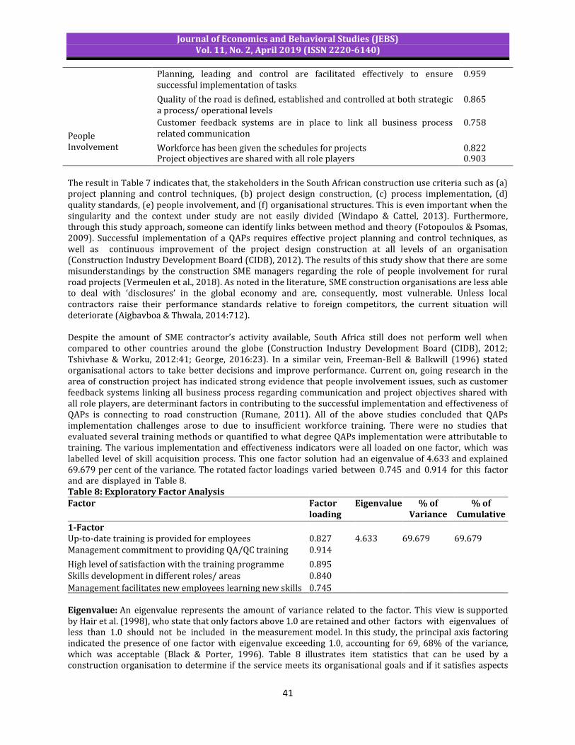
Journal of Economics and Behavioral Studies (JEBS) Vol. 11, No. 2, April 2019 (ISSN 2220-6140)
41
Planning, leading and control are facilitated effectively to ensure successful implementation of tasks
0.959
Quality of the road is defined, established and controlled at both strategic a process/ operational levels
0.865
People Involvement
Customer feedback systems are in place to link all business process related communication
0.758
Workforce has been given the schedules for projects 0.822 Project objectives are shared with all role players 0.903
The result in Table 7 indicates that, the stakeholders in the South African construction use criteria such as (a) project planning and control techniques, (b) project design construction, (c) process implementation, (d) quality standards, (e) people involvement, and (f) organisational structures. This is even important when the singularity and the context under study are not easily divided (Windapo & Cattel, 2013). Furthermore, through this study approach, someone can identify links between method and theory (Fotopoulos & Psomas, 2009). Successful implementation of a QAPs requires effective project planning and control techniques, as well as continuous improvement of the project design construction at all levels of an organisation (Construction Industry Development Board (CIDB), 2012). The results of this study show that there are some misunderstandings by the construction SME managers regarding the role of people involvement for rural road projects (Vermeulen et al., 2018). As noted in the literature, SME construction organisations are less able to deal with ‘disclosures’ in the global economy and are, consequently, most vulnerable. Unless local contractors raise their performance standards relative to foreign competitors, the current situation will deteriorate (Aigbavboa & Thwala, 2014:712). Despite the amount of SME contractor’s activity available, South Africa still does not perform well when compared to other countries around the globe (Construction Industry Development Board (CIDB), 2012; Tshivhase & Worku, 2012:41; George, 2016:23). In a similar vein, Freeman-Bell & Balkwill (1996) stated organisational actors to take better decisions and improve performance. Current on, going research in the area of construction project has indicated strong evidence that people involvement issues, such as customer feedback systems linking all business process regarding communication and project objectives shared with all role players, are determinant factors in contributing to the successful implementation and effectiveness of QAPs is connecting to road construction (Rumane, 2011). All of the above studies concluded that QAPs implementation challenges arose to due to insufficient workforce training. There were no studies that evaluated several training methods or quantified to what degree QAPs implementation were attributable to training. The various implementation and effectiveness indicators were all loaded on one factor, which was labelled level of skill acquisition process. This one factor solution had an eigenvalue of 4.633 and explained 69.679 per cent of the variance. The rotated factor loadings varied between 0.745 and 0.914 for this factor and are displayed in Table 8. Table 8: Exploratory Factor Analysis Factor Factor
loading Eigenvalue % of
Variance explained
% of Cumulative
1-Factor Up-to-date training is provided for employees 0.827 4.633 69.679 69.679 Management commitment to providing QA/QC training 0.914
High level of satisfaction with the training programme 0.895 Skills development in different roles/ areas 0.840
Management facilitates new employees learning new skills 0.745 Eigenvalue: An eigenvalue represents the amount of variance related to the factor. This view is supported by Hair et al. (1998), who state that only factors above 1.0 are retained and other factors with eigenvalues of less than 1.0 should not be included in the measurement model. In this study, the principal axis factoring indicated the presence of one factor with eigenvalue exceeding 1.0, accounting for 69, 68% of the variance, which was acceptable (Black & Porter, 1996). Table 8 illustrates item statistics that can be used by a construction organisation to determine if the service meets its organisational goals and if it satisfies aspects
Journal of Economics and Behavioral Studies (JEBS) Vol. 11, No. 2, April 2019 (ISSN 2220-6140)
42
such as planning process, skill acquisition, construction design, process implementation, organisational structure, quality requirements and people involvement. Furthermore, to justify these statements, these QAPs should be validated in a national study in order to ensure that they positively influence the successful delivery of road construction projects. 4. Conclusion and Recommendations In this study, the quality assurance practices of construction SMEs relating local governments of the Limpopo Province (South Africa) were analysed via a questionnaire created from a suitable context based on the Road Quality paradigm. The main conclusion to be drawn from this study is that there seven (7) QAPs to considered by SME contractors and local government managers that seek to identify and establish a road construction project effectively. These seven (7) critical aspects are indicated as latent constructs of the various individual areas identified in this study. Hence, this study concludes that the QAPs that should be considered by the SMEs contractors are (1) level of skill acquisition process factors; (2) project planning & control techniques; (3) project construction design; (4) process implementation & process improvement; (5) financial management skills; (6) organisational structures and involvement of people; (7) quality standards and measures. This finding seems to support similar findings by Gotzamani & Tsiotras (2001) that argues in favour of an appropriate quality standards contributing towards total quality management with technical approaches that can facilitate QAPs in the construction industry. Research literature reviewed highlights that identifying and establishing the impact of QA processes is the new paradigm in running construction projects within the South Africa construction industry, and attention should be given to the way in which its process are assigned, designed, implemented and maintained (George, 2016). For SME construction organisations to improve their road construction projects, owners or managers and their workforces need to implement QA processes effectively throughout the survey implementation. They need to simultaneously monitor, inspect and evaluate QA at both strategic and operational or process levels. Finally, clear targets for SME construction projects (see Table 8) is confirmed in the one out of seven factors as important aspect for QAPs implementation, which also confirmed by the existing literature (Kerzner, 2013; Rumane, 2011; Olawale & Sun, 2015; Obare et al., 2016; Panuwatwanich & Nguyen, 2017). Nevertheless, this study identified six other factors that seem to be equally significant in QAPs implementation. The results evidently indicated that quality of implementation leads to business growth, decrease of poor quality and improved customer satisfaction. In defining, analysing, implementing and evaluation processes of quality as well as effectiveness of road construction, the relationship between senior managers, consultants, workforces and customers remained significant for the success of the business. One major practical subject that has hampered road construction projects for many years is the unpredictability in project construction designs, thus creating impediments when implementing QA processes to the industry. Practical QA guidance for construction SMEs must be properly implemented and used efficiently. Quality improvement workshops must be provided for the required exceptional quality control of construction. Awareness, compliance and selfless adherence to quality standards must be measured regularly (Bierman et al., 2013; Martin & Lewis, 2014). Quality systems and standards need to be adopted in a way that will enable the organisation to meet its clients’ necessities (Honnakker et al., 2010). The study identifies critical core aspects contributing to practising and improving SMEs contractors’ performance. It also highlights what must be improved in relation to SMEs contractors, plans, systems, quality of implementation and organisational structure. The establishment of classy construction, analysis and QA processes using up-to-date scientific achievements are important in the construction project. Communicating effectively internally and externally can have positive impacts on the road quality building even in extreme conditions, reducing the whole life cycle costs of road re-engineering, and consequently, minimal traffic disruption. A good understanding of the impact of road construction SMEs in implementing successful quality assurance process and aligning organisational structures with QA processes in the local government construction as well as difficulties faces by SME road construction projects or municipal managers in South Africa was clearly identified and discussed in detail. The study recommends that SMEs contractors should ensure that quality of rural road infrastructure is implemented and that service quality measures in order to enhance the quality of roads that the municipality is providing in the local communities. The CIDB is main professional body of road construction projects in South Africa, thus public and private Chief Executives

Journal of Economics and Behavioral Studies (JEBS) Vol. 11, No. 2, April 2019 (ISSN 2220-6140)
43
Officers (CEOs) and project managers/administrators need to understand the importance of quality through the practice of evidence-road infrastructure. The project manager of a rural road project who wishes to assure and implement robust quality road infrastructure according to the processes of quality management should concentrate carefully on the seven critical aspects identified above. Project managers should first ensure that the SME contractors’ motivation for measuring the service quality is internally oriented, rather than being externally oriented. Further Areas of Research: Project managers in the rural road network infrastructure should perform check-ups, inquiries and applying remedial activities to enhance customers’ satisfaction that would bring long-term success and business certainty for the organisations (Bierman et al., 2013). It is important for municipal CEOs and project managers to know and understand how users and local community perceive the quality of the rural road construction projects as well as the service elements. Further study could determine that these reliable and valid QAPs can be used to successfully quality of roads infrastructure in construction projects undertaken by construction SMEs. However, study recommends research involving the private sector in sponsoring rural road construction projects through public-private partnerships. Future studies could employ a more rigid research methodology to implement sustainable QA process efficiency to achieve an improved road quality task at the local government level. Furthermore, to justify these statements, these QAPs should be validated in a national study in order to ensure that they positively influence the successful delivery of road construction projects. This study can also be conducted in other African countries for comparative purposes. References Ahadzie, D. K., Proverbs, D. G. & Olomolaiye. (2007). Critical success criteria for mass housing building
projects in developing countries. International Journal of Project Management, 34, 806-818. Aigbavboa, C. O. & Thwala, W. D. (2014). Challenges faced blacked owned small and medium construction
companies: A case study of Nelspruit-Mbombela Municipality, South Africa. Journal of Economics and Behavioural Studies, 6(10), 771-778.
Arditi, D. & Gunaydin, H. M. (1997). Total quality management in the construction process. International Journal of Project Management, 15(4), 235-243.
Aziz, R. F. & Abdel-Hakam, A. A. (2016). Exploring delay causes in road construction projects in Egypt. Alexandria Engineering Journal, 55, 1515-1539.
Badu, E. & Owusu-Manu, D. (2011). An overview of construction activities in Kumasi, in Adarkwa, K.K. (Ed). The Future of the Tree-Towards Development and Growth, 1st, 270-289.
Basu, R. (2004). Implementing quality: A practical guide to tools and techniques, enabling the power of operational excellence. UK: Thompson.
Bierman, M., Marnewick, A. & Pretorius, J. H. C. (2013). Productivity management in the South African civil construction industry-factors affecting construction productivity. Journal of the South African Institution of Civil Engineering, 58(3), 37-44.
Construction Industry Development Board (CIDB). (2012). The construction industry as a vehicle for contractor development and transformation.
Dangalazana, T. & Newadi, M. R. (2005). An exploratory study into the challenges facing the emerging contractors involved in the construction of low cost housing in Wells Estate and Ikamv’elihle Townships in the Nelson Mandela Metropolitan, South Africa. World Congress on Housing: Transforming Housing Environment through Design, 27-30.
Fang, D. & Wu, H. (2013). Development of a safety climate interaction (SCI) model for construction projects. Safety Science, 57, 138-149.
Field, A. (2013). Discovering statistics using IBM SPSS statistics. 4th Ed. Thousand Oaks, CA. SAGE Publication. Fotopoulos, C. B. & Psomas, E. L. (2009). The impact of “soft” and “hard” TQM elements on quality
management results. International Journal of Quality & Reliability Management, 26(2), 150-163. Freeman-Bell, G. & Balkwill, J. (1996). Management in engineering: Principles and practice. UK: Prentice-Hall. Gardiner, P. D. (2005). Project Management: A Strategic Planning Approach. UK: Palgrave MacMillan Ltd. George, H. (2016). Eliciting the financial challenges facing emerging contractors in developing countries using
the critical incident technique: A case of South African construction industry. Business and Management Horizons, 4(2), 23-33.
Journal of Economics and Behavioral Studies (JEBS) Vol. 11, No. 2, April 2019 (ISSN 2220-6140)
44
Gotzamani, K. D. & Tsiotras, G. D. (2001). An empirical study of the ISO 9000 standards’ contribution towards total quality management. International Journal of Operations Production Management, 21(10), 1326-1342.
Hair, J. F., Black, W. C., Babin, B. J. & Anderson, R. L. (2014). Multivariate data analysis. 5th Ed. Upper Saddle River, NJ, USA: Prentice Hall.
Kaiser, H. (1994). An index of factorial simplicity. Psychometrika, 39, 31-36. Kam, K. J. & Hamid, A. H. A. (2014). The true motives behind the adoption of QLASSIC- CIS 7:2006. As a
quality assurance initiative in construction industry. International Journal of Quality & Reliability, 32(6), 603-616.
Honnakker, P., Carayon, P. & Loushine, T. (2010). Barriers and benefits of quality management in the construction industry: An empirical study. Total Quality Management, 21(2), 953-969.
Kerzner, H. R. (2013). Project management: A systems approach to planning, scheduling, and controlling. New Jersey, USA: John Wiley & Sons.
Krejcie, R. V. & Morgan, D. W. (1970). Determining sample size for research activities. Educational and Psychological Measurement, 30(3), 607-610.
Kruger, D., Ramphal, R. & Maritz, M. (2014). Operations Management. 3rd Ed. Cape Town: Oxford University Press Southern Africa.
Jarkas, A. M. & Younes, J. H. (2014). Principle factors contributing to construction delays in the State of Qatar. International Journal of Construction Project Management, 6(1), 39-62.
Leedy, P. D. & Ormrod, J. E. (2014). Practical Research: Planning and Design. 10th Ed. UK: Pearson. Mahmood, S., Ahmed, S. M., Panthi, K. & Kureshi, N. I. (2010). Determining the cost of poor quality and its impact on
productivity and profitability. Built Environment Project and Asset Management, 4(3), 296-311. Martin, A. & Lewis, M. (2014). Pinpointing safety leadership factors for safe construction sites in Trinidad and
Tobago. Journal of Construction Engineering and Management, 40(2), 040133046. Mofokeng, G. & Thwala, W. D. (2012). Mentorship programmes within the Small and Medium Sized Contractor
Development Programme: A case study of the Free State Province, South Africa. Journal of Economics and Behavioural Studies, 4(12), 712-722.
Nyakala, K. S., Vermeulen, A., Pretorius, J. H. C. & Munyai, T. (2017). Implementation of quality assurance practices and effectiveness of the road construction industry: A case of South African local municipalities. Proceedings of the 2017 Global Business and Technology Association Conference, 636-650.
Obare, J. O., Kyalo, D. N., Mulwa, A. S. & Mbugua, J. (2016). Implementation process of project control systems and performance of rural roads construction project in Kenya: Role of project team experience diversity. European Scientific Journal, 12(29), 408-422.
Olawale, Y. & Sun, M. (2015). Construction project control in the UK: Current practice, existing problems, and recommendations for future improvement. International Journal of Project Management, 33, 623-637.
Pallant, J. (2013). SPSS, Survival manual: A step-by-step guide to data analysis using IBM, SPSS. 5th ed. London: Allen & Unwin.
Panuwatwanich, K. & Nguyen, T. T. (2017). Influence of organisational culture on total quality management implementation and firm performance: Evidence from the Vietnamese construction industry. Management and Production Engineering Review, 8(1), 5-15.
Rumane, R. J. (2011). Quality management in construction projects. CRC Press Taylor & Francis Group, LCC. Statistics South Africa. (2017). Statistical release manufacturing: Production and sales (Preliminary) April 2017. Tabachnick, B. G. & Fidell, L. S. (2007). Using multivariate statistics. 5th Ed. Hillside, NS: Erlbaum. Teddlie, C. & Tashakkori, A. (2003). Handbook of Mixed Methods in social & behavioural research. SAGE
Publications International Educational and Professor Publisher Thousand Oaks. London. New Delhi. Thorpe, B., Summer, P. & Duncan, J. (1996). Quality Assurance in Construction. Surrey, UK: Gower Publishing Ltd. Tshivhase, L. & Worku, Z. (2012). Barriers toward the development of emerging contractors in the Limpopo
Province. African Journal of Science, Technology, Innovation and Development, 4(1), 41-62. Van Wyk, L. (2003). A review of the South African construction industry: Economic, regulatory and public
sector capacity influences on the construction industry. Pretoria: CSIR. Vermeulen, A., Nyakala, K. S. & Pretorius, J. H. C. (2018). Development of a road quality assurance
measurement tool in construction projects. Proceedings of the 2018 International Conference on Management of Technology (2018 IAMOT). Birmingham, England, 22-26, 1-14.
Windapo, A. O. & Cattel, K. (2013). The South African Construction Industry: Perceptions of key challenges facing its performance, development and growth. Journal of Construction in Developing Countries, 18(2), 65-79.

Journal of Economics and Behavioral Studies (JEBS) Vol. 11, No. 2, April 2019 (ISSN 2220-6140)
45
An Assessment of the Employee Job Satisfaction: Views from Empirical Perspectives
Albert Tchey Agbenyegah Durban University of Technology, Pietermaritzburg, South African
[email protected] Abstract: Job satisfaction stresses on the personal feelings within the job environment in relation to job assessment. Various academics and scientists studied in the past, the significant association between personal expectations and job satisfaction of employees. These past studies were based on the model of personality traits and other variables in determination of employee job satisfaction. This study is to assess the relationship and effect between independent and dependent variables. To ensure that the stated objectives are met, a 7 point Likert scale questionnaires were administered to 140 managers and non-manager employees. However, only 128 of the questionnaires were returned without errors and ready to go through the analysis processes. Data analysis was conducted in two phases namely the descriptive and inferential statistics. Descriptive analysis aided by the mean counts was applied in describing the empirical data; whereas the inferential statistics of Pearson’s chi-square test and ANOVA were utilized to determine the relationship and the effect of independent on the dependent variable. ANOVA was used to assess the effect of independent variables on the dependent variable. This empirical study demonstrates mix results through Pearson’s chi-square and ANOVA tests. WEP and employee status does not differ from EJS whereas employee position differs from EJS. The ANOVA test revealed a significant effect of WEP and EPS on EJS. The study revealed that SME owners in FB district municipality experienced very high entrepreneurial challenges in contrast to their counterparts in JTG district municipality. Given these findings, the author called on policymakers to prepare specific strategies and programs that motivate employees within the establishment. Keywords: Employee job satisfaction, employee status, employee working experience, job satisfaction, variables.
1. Introduction Employee Job Satisfaction (EJS) is associated with variables such as the nature of tasks, managerial quality, supervisor characteristics, pay packages, promotion opportunities, organizational features and the working climate, work experience and employee salaries of the organizations (Balcı 2011: 70; Panghal and Bhambu 2013). These variables are central to the survival of the organization; thus, the responsibility is on the employer to motivate employees towards job satisfaction. According to Herzberg (1966), it is befitting that employers motivate employees for job satisfaction and productivity. Several authors have alluded to a vast number of variables that influence job satisfaction (Ahmad and Yekta 2010; Nawab and Bhatti 2011; Kord and Tamini 2012; Jeet and Sayeeduzzafar 2014). For instance, a study by Ahmad and Yekta (2010) confirmed the notion that intrinsic and extrinsic variables impact employees’ job satisfaction. A similar study revealed that job satisfaction is possible in various sectors through employees’ personality traits, besides the characteristics of the job (Chang and Lee 2006). Early theorists, including Mayo (1945), indicated that variables relating to sociology and psychology affect employees’ work life and job satisfaction. EJS is an ongoing concern for organization’s that aim to achieve their objectives. Satisfying employees creates positive results of belonging and organizational ownership, positive well-being and personal commitment across the length and breadth of organizations (Saks 2006; Nadiri and Tanova 2010; Zeinabadi 2010). It is costly for organizations to not create a conducive workspace for employees (Tracey and Hinkin 2008). Lambert, Hogan and Barton (2001) state that organizations that are unable to guarantee employee satisfaction could trigger an exodus of employees seeking alternative employment. Nowadays various organizations operate in a poor economic climate. As such, management is unable to meet its mandate of providing goods and services with the view of satisfying its potential market share (Spagnoli, Caetano and Santos 2012). Researchers view employee retention and the ability to attract employees as vital to a successful organization (Sehunoe, Mayer and Viviers 2015). The primary focus of this empirical study was to assess the relationships and effects of different variable on EJS. EJS is referred to as the emotional state of employees towards their assigned tasks (Locke 1976; Huang, You and Tsai 2012). A study by Stander and Rothmann (2010 ) found that if employees are satisfied and motivated, their productivity increases.
Journal of Economics and Behavioral Studies (JEBS) Vol. 11, No. 2, April 2019 (ISSN 2220-6140)
46
It is therefore paramount to determine the relationships and effects of different variables in establishing EJS. A multitude of job-related traits in humans was researched by psychologists over the years and it was found that job satisfaction is critical for the improvement of employees’ societal health (Schneider and Vaught 1993). Drawing from these perceptions relating to personal commitment, it is important that employees be rewarded. The job satisfaction of employees is the focus of different variables, including economic and interpersonal activities, as well as the work climate (Herzberg 1966; Locke 1976 ). This paper focuses on some of these variables to determine their effect and relationship on EJS. Job Satisfaction: Job satisfaction is defined as any form of enjoyment experienced by individuals in the achievement of specific tasks (Saeed et al., 2014). Robbins and Judge (2013) posit that job satisfaction focuses on the positive feelings towards a job through the motivation of employees. An earlier definition of job satisfaction by Locke (1976) referred to it as the interplay of human thoughts as expressed through the positive feelings of employees. Drawing from Locke’s (1976) definition, other researchers have stated that the concept of job satisfaction could be linked to three multidimensional concepts, namely the cognitive, effective, as well as behavioral elements of individuals as they perform specific tasks (Hoppock 1935; Hulin and Judge 2003 ). A study by Kyule, Katunzi and Arasa (Kyule, Katunzi and Arasa 2016) indicated that once employees are motivated, their levels of performance increase; thus, reducing absenteeism and encouraging retention in the workplace (Sukriket 2015). Job satisfaction, according to empirical studies, emphasizes the needs of employees, while taking into consideration strategies that govern the organization in reducing the dissatisfaction of employees (Uduji 2013). Within an organization, productivity is most likely to increase if employees’ behavior patterns change as a result of motivation; this, according to researchers, is linked to EJS (Yadav and Aspal 2014; Tufail, Muneer and Manzoor 2016; Tehseen and UI Hadi 2015). Employee Job Satisfaction (EJS): EJS refers to the general state of completeness that employees experience from assigned tasks in relation to a specific job. To ensure total employee satisfaction, the onus is on employers to design the quality of processes, including the physical environment, in the organization (Celik 2008). The concept of job satisfaction entails dissimilarities between the twin terms of “inputs” and “outputs”. These terms determine the exact employees’ inputs for positive job outputs; hence, any output of negative results represents employees’ dissatisfaction (Vishwakarma, Shukla and Nougriaya 2015 ). Other variables are connected to job satisfaction or dissatisfaction. According to Mahmoud (2008), the general expectations by the employees towards specific tasks in the organization contribute to job satisfaction. Jiang, Baker and Frazier (2009) posit that elements of poor performance levels in an organisation, standardized disorder operations and sub-standard quality products are some of the characteristics of dissatisfaction. While there is a lack of agreement on defining job satisfaction, scientific evidence indicates that through minimal process design costs and making available intrinsic payments packages to employees, job satisfaction increases (Parvin and Kabir 2011). Moreover, job satisfaction offers employees with multiple employee benefits. For example, by being satisfied with assigned tasks, the employee performs the tasks with a positive mindset, focusing on providing adequate “inputs” to increase productivity (Maher 2008). Theoretical Framework: According to McShane and Von Glinov (2007 in MacKain et al. (2010), several theories are used to define employee satisfaction in a global context. For example, George and Jones (1999) describe job satisfaction as including variables such as societal influence, personal characteristics, and workplace characteristics and values. In the context of psychology, Meyer and Allen (1991) define job satisfaction as continued commitment, as well as normative commitment. These theories enable researchers and academics to obtain a sense of the various dimensions of job satisfaction. As a result, other variables of importance contribute to assessing the employee-employer relationship. Furthermore, the effects of variables on job satisfaction are critical. These variables are diverse in a theoretical context; thus, this study foregrounds the expectancy and equity theories. The equity theory is focused on existing conditions, and not on set standards in terms of the conditions offered to employees in exchange for any form of reward by the employer (the principle of “inputs” and “outputs” applies). Thus, employers are obliged to exercise equal treatment and motivate employees to spur the level of organisational performances. The equity theory measures employees “inputs” against the “outputs”. This theory emphasizes employees’ perceptions regarding fair treatments by employers (Daft and Noel 2001). One of the outstanding features of the theory is the notion that employees make comparisons about the nature of their jobs and rewards.

Journal of Economics and Behavioral Studies (JEBS) Vol. 11, No. 2, April 2019 (ISSN 2220-6140)
47
The central tenet of the expectancy theory is the need for performance satisfaction of employees. According to Vroom (1964), in order for employees to be satisfied, every effort should trigger a reward in return. Thus, individual expectations in line with specific jobs are likely to increase or decrease performance. Hence, while it is known that some employees perform better based on individual returns, it is pivotal that in the end performance levels are expected to increase. The primary guiding principle of the expectancy theory entails understanding the aims of employees and the general linkages between performance and employees’ efforts, the inherent reward systems, and performance and employees’ desire to satisfy the goals of employees through adequate reward systems. Therefore, it is significant to measure the relationships and effects of variables on EJS. EJS is not equal, based on individuals’ needs and expectations, as well as other conditions within the organisation. Drawing from past scientific evidence, the present empirical study is to assess and suggest practical solutions. 2. Literature Review Work Experience: Brief (Brief 1998) suggested that job satisfaction represents different results, as well as the conditions that are expressed to form the basis to perform duties. In instances where individual job performance is good, fair compensation is demanded, with a good chance of promotion. These strings of events call for an employee to be satisfied. Variables such as the physical climate, task fulfilment and quality relationships can impact on an employee’s assigned tasks despite experience (Rode 2004). The number of years employees spend in an organisation is significant to make a determination in relation to job satisfaction. The number of years spent in a job is used as the chief predictor for job satisfaction. According to Oshagbemi and Hickson (2003), working for a shorter period could lead to dissatisfaction in a specific organisation, in contrast to working for a longer period. In a similar study, Martin and Roodt (2008) found that employees show higher levels of satisfaction if more years are spent in an organisation. Sharma and Jyoti (2009) posit that employee satisfaction is minimal within the first five years in a job; however, they add that employee satisfaction increases if an individual works for over 20 years in an organisation. Kumar and Giri (2009) concurred that there is a relationship between job satisfaction and work experience. According to the study, employees’ levels of satisfaction increased if they worked for the organisation for longer periods. The study concluded that the work experience of an employee impacts positively on job satisfaction. Ercikti et al. (2011) were in agreement that among all the demographic variables, the period of years an employee worked in an organisation determines his/her job satisfaction. They, however, found that employees who were newly employed enjoyed higher job satisfaction in comparison to employees who had worked for several years. In light of the empirical and literature studies, the following null hypotheses were formulated: HN: Working experience has no significant effect on employee satisfaction. HN: There is no significant relationship between working experience and EJS. Employment Status: This study categories employment status into permanent and contract employment. Throughout this study, contract and temporary employment are used interchangeably. Empirical studies have shown vast distinctions between permanent and contractual types of employment. Based on employment principles, temporary employees either enjoy negative or positive job satisfaction. Studies have revealed that employees create extra insecurity impairments that lead to dissatisfaction. Indicated, that as job insecurity worsened, the general lack of employees’ well-being resulted in negative feelings towards their jobs due to dissatisfaction. These negative events in organisation harmed employer-employees’ contractual relationships (Rousseau 1995). According to Davy, Kinicki and Scheck (1997), there is a significant relationship between job security and employment status. For instance, higher employee status is likely to be autonomous, challenging, and have greater responsibilities and opportunities, which implies that employees enjoy job satisfaction (Schultz and Schultz 2006). The study further found that the technical, managerial and professional status of employees attracts higher EJS, in contrast to other sectors where this was not present. However, evidence indicated that EJS differs in terms of assigned jobs rankings (Witte 1999). Scientific evidence has revealed a distinction between permanent and contract employment. Employees who are permanently employed are perceived to belong to the organisation, in contrast to contractual employees (De Cuyper, De Witte and Isaksson 2005 ).
Journal of Economics and Behavioral Studies (JEBS) Vol. 11, No. 2, April 2019 (ISSN 2220-6140)
48
No matter the level of differences in the job satisfaction of employees, permanent employees are said to be periphery workers once they are allocated to contractual tasks. According to Guest et al. (Guest et al., 2006), once contractual employees realize that employers do not value their tasks in the organisation, they become dissatisfied. However, temporary employees are essential to organizations. Temporary employees are perceived as the salient assets in all forms of organisations as their contributions are valuable (Connelly, Gallagher and Gilley 2007). By inferring from empirical evidence and literature, the following null hypotheses were stated: HN: Employee status has no significant effect on employee satisfaction. HN: There is no significant relationship between employee status and EJS. Employee Position: Within an organisation, employees hold several positions of value. These positions are hierarchically structured in accordance with the dictates of the organisation. There is the general perception that individual positions could impact on job satisfaction (Schultz and Schultz 2006). Hancer and George (2003) concurred that there are significant linkages between an employee’s position in the organisation and job satisfaction. Drawing on Herzberg’s theory, it could be stated that for an individual to experience satisfaction, variables such as the content and context is of significance in making employees feel satisfied. The study further stressed that these feelings by employees in senior positions can be attributed to variables, such as the existing work climate and supervision, autonomy, responsibility, as well as higher pay packages and promotion. Employee position within an organisation is regarded as one of the variables that impact job satisfaction (Schulz 2013). In a similar study by, it was established that there are differences in terms of employee motivation and positions; the highest motivators are found in the middle and senior levels of the hierarchy, whereas non-managers are less motivated. Similarly, stated that the promotion to a higher rank within an organisation presents enormous responsibilities for aspiring employees to pursue other related tasks. Shodhganga (2012) concurred that employees experienced more satisfaction than their peers once they assumed a higher position within an organisation. An empirical study by Kinzl et al. (2005) confirmed that high-ranking positions within an organisation are associated with job satisfaction. Furthermore, Theodossiou, Zangelidis and (2009) echoed the general sentiment that the position held by an employee in an organisation in many ways affected job satisfaction. The study further revealed that employers needed to make it possible for employees to follow career paths. According to Bates (2006), employers are expected to provide employees with senior level promotion opportunities. Drawing on the expectancy theory of, it can be said that the position held by an employee could motivate or demotivate him/her. Research by Waskiewicz (1999: 70) suggests that any position within an organisation should be designed to increase an employee’s level of performance. Hence, the inability of employees to perform as expected threatened their performance. It could be viewed as a punitive measure to demotivate employees in the absence of optimum levels of performances (Van Dalen and Henkens 2013). Building on both empirical evidence and the literature review, the researcher hypothesised the null hypotheses as follows: HN: Present position of employee has no significant effect on employee satisfaction. HN: There is no significant relationship between present position and EJS. The Proposed Conceptual Framework: Figure 1 below depicts the conceptual framework that directs this empirical study. This framework was based on the prior scientific work of Ivancevich. The primary aim of the framework was threefold: to support, build and test formulated hypotheses. Independent variables used in this study fell in three categories, namely Personal/Individual variables (work experience), Organisational variables (employee position), and Demographic variables (employment status). In addition, the framework illustrates the dependent variable, Employee Job Satisfaction (EJS). All these variables were operationalised and defined earlier, in line with this study. While the three independent variables mentioned may have a direct relationship and effect on EJS, their levels of weighting may differ. As such, this study postulates, as indicated through the hypotheses. 3. Research Methodology The researcher designed this study to ascertain quantitative data using a structured questionnaire. This study utilised a quantitative format as the statistical tools of ANOVA and Pearson’s chi-square test had to be

Journal of Economics and Behavioral Studies (JEBS) Vol. 11, No. 2, April 2019 (ISSN 2220-6140)
49
conducted to either accept or reject the formulated hypotheses in line with variables, such as work experience, employee status, employee position and EJS. By gathering primary data through the quantitative method, the researcher was of the opinion that the research objectives of assessing the significant differences and the effect of the variables would be met. Figure 1: Conceptual Framework Independent variables Dependent variable H1 H2 H3 Source: Empirical study (2018) Data Collection: The primary data for this study was gathered from respondents within organisation X in South Africa. The actual name of the research setting is withheld for ethical purposes. The researcher made the decision not to limit the target population for two reasons: to cover a larger group of respondents in search of credible data, and to produce a reliable and comprehensive research report. The target population consisted of permanent employees across six departments of the organisation. The justification for gathering data from only permanent employees was to allow the researcher to source primary data from the employees who were not only secure in the organization but worked under similar work conditions and enjoyed equal rights and opportunities. Due to the geographical nature of the research settings, convenience sampling technique was utilised to sample all the respondents (Blumberg, Cooper and Schindler 2011). Convenience sampling was employed to ensure that the researcher could easily access a larger group of permanent employees within a limited time frame, for a high level of anonymity, and to allow the respondents to easily complete the questionnaire at their own pace. Research Instrument: This study was quantitative and based on previous scientific work. The author designed a 7- point Likert scale using a 25 item scale with alterations from Mehrabani and Shajari (2013) . In the end, these scales were relevant enough to gather credible primary data. To ensure that the scales fitted the present context and the research aims, the research variables were assessed through a 7-point Likert scale. The scales were ranged from (7) strongly disagree to (1) strongly agree. In total, 140 questionnaires were distributed. However, only 128 were returned without errors, with a response rate of 91%. Prior to administering the research instruments, the questionnaires were piloted on a few respondents and experts (Saunders, Lewis and Thornhill 2012 ). Thereafter, the researcher made the necessary alterations for clarity. Data analysis was conducted by means of descriptive statistics using the mean values and two inferential statistics of Pearson’s chi-square test and ANOVA. The reliability and consistency of the questionnaires were measured by Cronbach alpha. The Cronbach alpha was utilised to measure 25 items that yielded 0.76 and 0.84 respectively of the applicable variables. According to Sekaran and Bougie (2016), the Cronbach alpha determines a set of variables of a latent construct. Thus, the results were an indication that all the items specified on the questionnaires were reliable and consistent (Brown 2002) .
Organisational variable
Employee position
Employee Job
Satisfaction
(EJS)
Demographic variable
Employment status
Personal/individual
variable
Work experience

Journal of Economics and Behavioral Studies (JEBS) Vol. 11, No. 2, April 2019 (ISSN 2220-6140)
50
Data Analysis and Results: For the sake of clarity and to attain the set objectives, descriptive statistics (mainly the mean values) were employed for a meaningful presentation of the empirical data set. In addition, inferential statistical tools (namely, the Pearson’s chi-square test and ANOVA) were applied to assess the relationship and effect of independent and dependent variables (refer to Figure 1). The tests were in line with the principle of a “significance level of 0.05(5%)”. The null hypotheses were not accepted in cases where the p-value yielded less than the significant level of 0.05. Through the inferential statistics, the researcher was able to either reject or support the formulated hypotheses. Descriptive Analysis: Different descriptions relating to the respondents in terms of biographical profiles on work experience, employees’ status, and present position are shown in Tables 1, 2 and 3 below. Table 1: Employee Satisfaction by Work Experience
Work experience N Mean
Std. Deviation
Std. Error
95% Confidence Interval for Mean
Min Max Lower Bound
Upper Bound
< 1 year 3 30.00 21.284 12.288 -22.87 82.87 7 49
>1-3 years 40 19.85 10.812 1.710 16.39 23.31 7 44
>4-5 years 42 16.48 10.322 1.593 13.26 19.69 7 42
>6-10 years 25 23.88 13.252 2.650 18.41 29.35 7 49
>10 years 7 29.14 11.452 4.328 18.55 39.73 13 42 The table above indicates that employees who worked for less than one year enjoyed the highest level of job satisfaction (mean=30), while employees who worked between four and five years experienced the lowest level of job satisfaction (mean=16.48). The results from the table indicated that 42 (36%) of the participants, with over four years of work experience, were less satisfied. This implied that the level of work experience did not relate or affect job satisfaction in the organization. Table 2: Employee Satisfaction by Employee Status
Employee status
N Mean Std. Deviation
Std. Error
95% Confidence Interval for Mean
Min Max Lower Bound
Upper Bound
Permanent 80 19.25 11.884 1.329 16.61 21.89 7 49
Contract 37 22.78 12.118 1.992 18.74 26.82 7 49
The table above shows that among the respondents, employees on contract enjoyed the highest level of employee job satisfaction (mean=22.78), in contrast to permanent employees who enjoyed a minimal level of job satisfaction (mean=19.25). Table 3: Employee Satisfaction by Present Position
Present Position
N Mean Std. Deviation
Std. Error
95% Confidence Interval for Mean
Min Max Lower Bound
Upper Bound
Managerial 7 29.14 12.048 4.554 18.00 40.28 17 46
Supervisory 8 9.13 2.900 1.025 6.70 11.55 7 15
Officer 37 15.22 9.883 1.625 11.92 18.51 7 42
Junior Staff 66 23.83 11.820 1.455 20.93 26.74 7 49
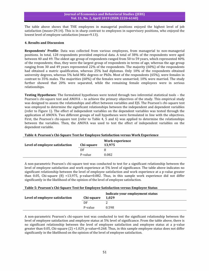
Journal of Economics and Behavioral Studies (JEBS) Vol. 11, No. 2, April 2019 (ISSN 2220-6140)
51
The table above shows that THE employees in managerial positions enjoyed the highest level of job satisfaction (mean=29.14). This is in sharp contrast to employees in supervisory positions, who enjoyed the lowest level of employee satisfaction (mean=9.13). 4. Results and Discussion Respondents’ Profile: Data was collected from various employees, from managerial to non-managerial positions. In total, 128 respondents provided empirical data. A total of 38% of the respondents were aged between 40 and 49. The oldest age group of respondents ranged from 50 to 59 years, which represented 40% of the respondents; thus, they were the largest group of respondents in terms of age, whereas the age group ranging from 30 and 49 years represented 22% of the respondents. The majority (60%) of the respondents had obtained a matric qualification, whereas 25% had diplomas. Only 10% of the respondents obtained university degrees, whereas 5% held MSc degrees or PhDs. Most of the respondents (65%), were females in contrast to 35% males. The majorities (60%) of the females were unmarried; 10% were married. The study further showed that 20% were separated, while the remaining female employees were in serious relationships. Testing Hypotheses: The formulated hypotheses were tested through two inferential statistical tools – the Pearson’s chi-square test and ANOVA – to achieve the primary objectives of the study. This empirical study was designed to assess the relationships and effect between variables and EJS. The Pearson’s chi-square test was employed to determine the significant relationships between the independent and dependent variables (refer to Figure 1). The effect of independent variables on the dependent variables was tested through the application of ANOVA. Two different groups of null hypotheses were formulated in line with the objectives. First, the Pearson’s chi-square test (refer to Table 4, 5 and 6) was applied to determine the relationships between the variables. Then, the ANOVA was used to test the effect of independent variables on the dependent variable. Table 4: Pearson’s Chi-Square Test for Employee Satisfaction versus Work Experience
Work experience Level of employee satisfaction Chi-square 13,975
DF 8
P-value 0.082
A non-parametric Pearson’s chi-square test was conducted to test for a significant relationship between the level of employee satisfaction and work experience at 5% level of significance. The table above indicates no significant relationship between the level of employee satisfaction and work experience at a p-value greater than 0.05, Chi-square (8) =13,975, p-value=0.082. Thus, in this sample work experience did not differ significantly in the likelihood of the opinion of the level of employee satisfaction. Table 5: Pearson’s Chi-Square Test for Employee Satisfaction versus Employee Status
Indicate your employment status Level of employee satisfaction Chi-square 1,029
DF 2
P-value 0.598
A non-parametric Pearson’s chi-square test was conducted to test the significant relationship between the level of employee satisfaction and employee status at 5% level of significance. From the table above, there is no significant relationship between the level of employee satisfaction and employee status at a p-value greater than 0.05, Chi-square (2) =1.029, p-value=0.268. Thus, in this sample employee status does not differ significantly in the likelihood on the opinion of the level of employee satisfaction.

Journal of Economics and Behavioral Studies (JEBS) Vol. 11, No. 2, April 2019 (ISSN 2220-6140)
52
Table 6: Pearson’s Chi-Square Test for Employee Satisfaction versus Present Position
Present position Level of employee satisfaction Chi-square 19,807
DF 6
P-value 0.003
A non-parametric Pearson’s chi-square test was conducted to test the significant relationship between the level of employee satisfaction and the present position at a 5% level of significance. From the table above, there is a significant relationship between the level of employee satisfaction and the present position at a p-value less than 0.05, Chi-square (6) =19.807, p-value=0.003 Thus, in this sample the present position differs significantly in the likelihood on the opinion of the level of employee satisfaction. Testing Hypotheses: This section used the ANOVA technique to test the hypotheses to make inferences in line with the conceptual framework (Figure 1). The aim was to achieve the primary objective of determining the impact of independent variables on EJS. Tables 7, 8 and 9 below reveal how the independent variables impact on EJS. Table 7: ANOVA Test for Effect of Employee Work Experience on EJS
Sum of Squares DF Mean Square F P-value Between Groups 1772.226 4 443.056 3.345 0.013
Within Groups 14835.073 112 132.456
Total 16607.299 116
A one-way ANOVA was conducted at 5% level of significance to test the significant effect of work experience on employee satisfaction: less than one year, one to three years, four to five years, six to ten years, and more than ten years’ experience. Based on the table above, the researcher found that there was a significant effect of work experience on employee satisfaction at p<0.05 for the five conditions [F (4,112) =3.345, p=0.013]. The null hypothesis (HN), is rejected at 5% level of significance. Table 8: ANOVA Test for Effect of Employee Status on EJS
Sum of Squares DF Mean Square F p-value Between Groups 315.926 1 315.926 2.210 0.140
Within Groups 16443.270 115 142.985
Total 16759.197 116
A one-way ANOVA was conducted at 5% level of significance to test the significant effect of employee status on employee satisfaction, and permanent and contract conditions. The table above revealed no significant effect of employee status in terms of employee satisfaction at p>0.05 for the two conditions [F (1,115) =2.210, p=0.140]. The null hypothesis (HN), is not rejected at 5% level of significance. Table 9: ANOVA Test for Effect of Employee’s Present Position on EJS
Sum of Squares DF Mean Square F p-value Between Groups 3324.026 3 1108.009 9.338 0.000
Within Groups 13527.169 114 118.659
Total 16851.195 117

Journal of Economics and Behavioral Studies (JEBS) Vol. 11, No. 2, April 2019 (ISSN 2220-6140)
53
A one-way ANOVA was conducted at 5% level of significance to test the significant effect of the present position of the employee on the level of employee satisfaction relating to managerial, supervisory, officer and junior staff conditions. The results as stated in the table showed a significant effect on the present position of the employee on employee satisfaction at p<0.05 for the four conditions (F (3,114) =9.338, p=0.000]. The null hypothesis (HN), is rejected at 5% level of significance. Tables 10, 11 and 12 below depict the practical presentations of the research findings in line with the study objectives. Table 10: Graphic Presentations of Empirical Findings (Descriptive Statistics)
Table 11: Graphic Presentation of Empirical Findings (Pearson’s Chi-square Test) Independent variables Results Statistics/Hypotheses Work experience (WEP) No relationship WEP does not differ from EJS Employee status No relationship Employee’s status does not differ from EJS Employee position There is a relationship Employee’s position differs from EJS Table 12: Graphic Presentations of Empirical Findings (ANOVA) Independent Variables Results Statistics/Hypotheses Work experience Significant effect of WEP on EJS Hn: Is rejected at 5% level of significance Employee status (EPS) No significant effect of EPS on EJS Hn: Is not rejected at 5% level of
significance Employee position (EPO) Significant effect of EPO on EJS Hn: Is rejected at 5% level of significance Discussion of Results: The study sought to assess the significant relationships and effects between independent variables (work experience, employee status and position) and the dependent variable (EJS). Employee satisfaction in organisations differs. Job satisfaction, in general, depends on several variables. However, despite difficult working conditions, employees are expected to perform in line with employees’ expectations to meet set objectives. To ensure employees are satisfied, this empirical study utilised two inferential statistical tools; namely, Pearson’s chi-square test and ANOVA, to conduct the statistical analysis. Regarding the socio-demographic profile of the participants, the study showed that 40% were in the age group ranging from 50 to 59 years, 38% were aged 40 years and above, while 22% were aged between 30 and 49 years. The participants’ age in this study cannot be overlooked as every participant’s age relates to specific needs and expectations in line with social needs, as well as conditions of employment. Literature indicates that the age of participants plays a significant role in EJS. For instance, the U-shaped theory of Clark (1997) indicates the relationship between EJS and the lifespan of employees. The theory further adds that older employees are more satisfied in contrast to younger employees in an organisation. The management must endeavour to increase the level of employee satisfaction; if employees are satisfied in their jobs, employee turnover will decrease as employees gain more experience in the organisation with a resultant effect on productivity. Results in terms of academic achievements showed that 65% of the respondents had matric qualifications, 25% obtained diplomas, while 5% held university degrees, and another 5% obtained MSc degrees and PhDs. To a certain extent, this result indicates a high level of literacy in the organisation. This finding is consistent with a study by (Hoy and Musker 1987) which indicated that highly qualified employees are better positioned to find better employment and experienced sufficient satisfaction in contrast to less qualified employees. Most of the respondents were females, with the majority (60%) not being married. Ten percent were married and 20% were separated. The result implied that the most of the respondents did not have could concentrate on their jobs as most of them were unmarried. A total of 70
Independent Variables Results Statistical/Hypotheses Work experience (WEP) (less than one year) very satisfied Mean value 30. Work experience (4 years and above) least satisfied Mean value 16.48 Employee status (EPS): Contract Very satisfied Mean value 22.78 Employee status: Permanent Minimal satisfaction Mean value 19.28 Employee position (EPO): Managerial High satisfaction Mean value 29.14 Employee position: Supervisory Least satisfied Mean value 9.13 Junior and other officers More satisfied than supervisors Mean value 23.83/15.22
Journal of Economics and Behavioral Studies (JEBS) Vol. 11, No. 2, April 2019 (ISSN 2220-6140)
54
(60%) of the matric certificate holders were employed in permanent positions, while 47 (40%) held contract appointments in the organisation. The empirical outcomes of this study showed that the null hypotheses for employee experience (HN1) employment status (HN2) and employee position (HN3) were inconclusive as two null hypotheses are accepted and only one is rejected. Through the ANOVA technique, it was found that there is a significant effect of two key independent variables out of the three variables earmarked for the study. The independent variables are work experience and employees in a permanent position. The findings are inconsistent with a study by Oshagbemi and Hickson (2003) that employees who worked in organisations for a few years were highly dissatisfied in contrast to those who worked for a longer period in organisations. 5. Conclusion and Recommendations This empirical study was designed to assess the relationships between work experience, employee position and employee status, and the dependent variable of EJS. Specifically, the study sought to determine whether there was a significant effect between independent and dependent variables. To contextualize this study, an extensive literature search was conducted on the various independent variables, such as work experience, employee position and employment status. Through the literature review, broader insights on the research phenomenon were obtained, with more focus on the dependent EJS. At the same time, related gaps in the existing literature were uncovered. Inferences from the primary data were possible through two statistical tools – the ANOVA and Pearson’s chi-square test. Having completed the analysis, the study revealed that the dependent variable of EJS did not support the two independent variables of WEP and employee status. Moreover, no relationship existed between the variables. However, there was a relationship between employee position and EJS. The ANOVA statistical tool, based on the formulated hypotheses, showed mix findings in terms of the dependent variable of EJS, as well as the independent variables of EPS, WEP and EPO. Two variables, WEP and EPO, were found to have a significant effect on EJS, whilst EPS did not have a significant effect. Hence, two null hypotheses were rejected. Only one was accepted, as indicated in Table 12. Given the rural nature of the study area, these results were of significance as they indicated the effect and relationship of independent variables on EJS. The mean results (Table 10) of the independent variables were discussed. The findings pointed to high levels of dissatisfaction among junior employees, including those in managerial positions. Based on these findings, the following recommendations were made to enhance EJS. Provision of a well-structured system of recognition and rewards (rewards could be non-monetary or monetary). Management needs to institute employees’ assistance programmes (EAPs) to offer tailored-made support to employees in supervisory positions across departments. The EAPs should focus on the training needs of each employee in relation to his/her job description. The establishment of mentor programmes must be instituted to strengthen the subordinate-supervisor relationship. The establishment of an employee participation forum (EPF) across the organisation to involve employees to discuss issues that impact negatively on their performance. Implications: Given the high demand for job satisfaction by employees, the onus is on employers to identify variables that impact on EJS in their organisation. Once the level of impact is determined whether negative or positive, policymakers and managers need to craft tailored-made strategies and programmes to motivate their employees. These programmes and policies are desirable as job satisfaction within an organisation increases employees’ performance and ensures that the organisation’s stated objectives are met. Furthermore, this finding can be utilised as a key input in formulating strategies towards establishing workable policies in the organisation. EPF could increase individuals’ autonomy and controls of their personal lives, motivate them, increase their commitment to the organisation, and stimulate productivity. EPFs enable employees to become active participants in decision-making processes. Acknowledgements Compelling Interest: There was no inappropriate financial or personal interest on the part of the author in preparing this empirical study. Author’s Contributions: The author designed this study and developed it; assistance was sought from a statistician, L.S., to analyse the primary data.
Journal of Economics and Behavioral Studies (JEBS) Vol. 11, No. 2, April 2019 (ISSN 2220-6140)
55
References Ahmad, Z. A. & Yekta, Z. A. (2010). Relationship between perceived organizational support, leadership
behavior, and job satisfaction: An empirical study in Iran. Intangible Capital, 6 (2), 162-184. Balcı, F. (2011). The effects of education on police officer job satisfaction: a case of Turkish national police.
International Journal of Human Science, 8(2), 265-285. Bates, W. R. (2006). An investigation into the work environment elements on job satisfaction-a case study on
a company in the telecommunications industry. University of Johannesburg. Blumberg, B., Cooper, D. R. & Schindler, P. S. (2011). Business Research Methods. London: McGraw-Hill. Brief, A. P. (1998). Attitudes in and around organizations. Sage. Brown, J. D. (2002). The Cronbach alpha reliability estimate. JALT Testing & Evaluation SIG Newsletterrode, 6
(1). Celik, C. (2008). Relationship of organizational commitment and job satisfaction: A field study of tax office
employees. Chang, S. C. & Lee, M. S. (2006). Relationships among personality traits, job characteristics, job satisfaction
and organizational commitment–an empirical study in Taiwan. The Business Review, 6(1), 201-207. Clark, A. E. (1997). Job satisfaction and gender: Why are women so happy at work? Labour Economics, 4, 341–
372.10.1016/S0927-5371(97)00010-9. Connelly, C. E., Gallagher, D. G. & Gilley, K. M. (2007). Organizational and client commitment among contracted
employees: A replication and extension with temporary workers. Journal of Vocational Behavior, 70 (2), 326-335.
Daft, R. L. & Noel, R. A. (2001). Organisational Behaviour. New York: South-Western Publishing. Davy, J. A., Kinicki, A. J. & Scheck, C. L. (1997). A test of job security's direct and mediated effects on
withdrawal cognitions. Journal of Organizational Behavior: The International Journal of Industrial, Occupational and Organizational Psychology and Behavior, 18(4), 323-349.
De Cuyper, N., De Witte, H. & Isaksson, K. (2005). Temporary employment in Europe: Conclusions. In: De Cuyper, N., Isaksson, K. and De Witte, H. eds. Employment contracts and well-being among European workers. Hampshire, 225-244.
Ercikti, S., Vito, G. F., Walsh, W. F. & Higgins, G. E. (2011). Major Determinants of Job Satisfaction Among Police Managers. Southwest Journal of Criminal Justice, 8(1).
Guest, D. E., Oakley, P., Clinton, M. & Budjanovcanin, A. (2006). Free or precarious? A comparison of the attitudes of workers in flexible and traditional employment contracts. Human Resource Management Review, 16(2), 107-124.
Hancer, M. & George, R. T. (2003). Job satisfaction of restaurant employees: An empirical investigation using the Minnesota Satisfaction Questionnaire. Journal of Hospitality & Tourism Research, 27(1), 85-100.
Herzberg, F. (1966). Work and the nature of man, Cleveland World Publishing Co. Hoppock, R. (1935). Job satisfaction, Harper and Brothers, New York, 47. Hoy, W. & Musker, C. (1987). Educational administration: theory, research and practice. 3rd. ed. New York:
Random House. Huang, C. C., You, C. S. & Tsai, M. T. (2012). A multidimensional analysis of ethical climate, job satisfaction,
organizational commitment, and organizational citizenship behaviors. Nursing Ethics, 19(4), 513-529.
Hulin, C. L. & Judge, T. A. (2003). Job attitudes. In: Borman, W. C., Liken, D. R. and Klimoski, R. J. eds. Handbook of psychology: industrial and organisational psychology. Hoboken, NJ: Wiley, 255–276.
Jeet, V. & Sayeeduzzafar, D. (2014). A study of HRM practices and its impact on employees job satisfaction in private sector banks: A case study of HDFC Bank. International Journal of Advance Research in Computer Science and Management Studies, 2(1), 62-68.
Jiang, B., Baker, R. C. & Frazier, G. V. (2009). An analysis of job dissatisfaction and turnover to reduce global supply chain risk: Evidence from China. Journal of operations management, 27(2), 169-184.
Kinzl, J., Knotzer, H., Traweger, C., Lederer, W., Heidegger, T. & Benzer, A. (2005). Influence of working conditions on job satisfaction in anaesthetists. British Journal of Anaesthesia, 94(2), 211-215.
Kord, B. & Tamini, B. K. (2012). A cross-cultural study of job satisfaction and organizational commitment of bank employees in Iran and India. Apeejay Journal of Management and Technology, 7(1), 13-18.
Kumar, P. & Giri, V. N. (2009). Effects of age and experience on job satisfaction and organizational commitment. The Icfai University of Organizational Behavior, 8(1), 28-36.

Journal of Economics and Behavioral Studies (JEBS) Vol. 11, No. 2, April 2019 (ISSN 2220-6140)
56
Kyule, A. K., Katunzi, T. & Arasa, R. (2016). The moderating effect of remuneration on the relationship between work-life policies and employee work outcomes among lecturers in Kenya. Nairobi:
Lambert, E. G., Hogan, N. L. & Barton, S. M. (2001). The impact of job satisfaction on turnover intent: a test of a structural measurement model using a national sample of workers. The Social Science Journal, 38(2), 233-250.
Locke, E. A. (1976). The nature and causes of job satisfaction. In: Dunnette, M. D. ed. Handbook of Industrial and Organisational Psychology. Chicago, IL: Rand McNally.
MacKain, S. J., Myers, B., Ostapiej, L. & Newman, R. A. (2010). Job satisfaction among psychologists working in state prisons: The relative impact of facets assessing economics, management, relationships, and perceived organizational support. Criminal Justice and Behavior, 37(3), 306-318.
Maher, D. (2008). Interactive whiteboards and web conferencing systems in the primary school. Educational Research at Macquarie, 3, 30-31.
Mahmoud, A. (2008). A study of nurses' job satisfaction: the relationship to organizational commitment, perceived organizational support, transactional leadership, transformational leadership, and level of education. European journal of scientific research, 22(2), 286-295.
Martin, A. & Roodt, G. (2008). Perceptions of organisational commitment, job satisfaction and turnover intentions in a post-merger South African tertiary institution. SA Journal of Industrial Psychology, 34(1), 23-31.
Mayo, E. (1945). The Social Problems of an Industrial Civilization. Boston: School of Business Administration, Harvard University.
Mehrabani, S. E. & Shajari, M. (2013). Relationship between employee empowerment and employee effectiveness. Service Science and Management Research, 2(4), 60-68.
Meyer, J. P. & Allen, N. J. (1991). A three-component conceptualization of organizational commitment. Human resource management review, 1(1), 61-89.
Nadiri, H. & Tanova, C. (2010). An investigation of the role of justice in turnover intentions, job satisfaction, and organizational citizenship behavior in hospitality industry. International Journal of Hospitality Management, 29(1), 33-41.
Nawab, S. & Bhatti, K. K. (2011). Influence of employee compensation on organizational commitment and job satisfaction: A case study of educational sector of Pakistan. International Journal of Business and Social Science, 2(8)
Oshagbemi, T. & Hickson, C. (2003). Some aspects of overall job satisfaction: A binomial logit model. Journal of Managerial Psychology, 18(4), 357-367.
Panghal, S. & Bhambu, S. (2013). Factors influencing job satisfaction of banking sector employees in India. International Journal of New Innovations in Engineering and Technology, 1(3), 41-44.
Parvin, M. M. & Kabir, M. N. (2011). Factors affecting employee job satisfaction of pharmaceutical sector. Australian Journal of business and management research, 1(9), 113.
Robbins, S. & Judge, T. (2013). Organisational behavior 15th ed. Boston.: Pearson. Rode, J. C. (2004). Job satisfaction and life satisfaction revisited: A longitudinal test of an integrated model.
Human relations, 57(9),1205-1230. Rousseau, D. (1995). Psychological contracts in organizations: Understanding written and unwritten
agreements. Sage Publications. Saeed, I., Waseem, M., Sikander, S. & Rizwan, M. (2014). The relationship of turnover intention with job
satisfaction, job performance, leader-member exchange, emotional intelligence and organizational commitment. International Journal of Learning and Development, 4(2), 242-256.
Saks, A. M. (2006). Antecedents and consequences of employee engagement. Journal of managerial psychology, 21(7), 600-619.
Saunders, M., Lewis, P. & Thornhill, A. (2012). Research methods for business students. . New York: : Prentice Hall.
Schneider, D. S. & Vaught, B. C. (1993). A comparison of job satisfaction between public and private sector managers. Public Administration Quarterly, 68-83.
Schultz, D. & Schultz, S. E. (2006). Psychology and Work Today. 9th ed. New Jersey: Pearson Education Inc. Schulz, J. (2013). The impact of role conflict, role ambiguity and organizational climate on the job satisfaction
of academic staff in research-intensive universities in the UK. Higher Education Research & Development, 32(3), 464-478.
Journal of Economics and Behavioral Studies (JEBS) Vol. 11, No. 2, April 2019 (ISSN 2220-6140)
57
Sehunoe, N., Mayer, C. H. & Viviers, R. (2015). Job satisfaction, organisational commitment and work engagement in an insurance company. South African Journal of Labour Relations, 39(2), 123-144.
Sekaran, U. & Bougie, R. (2016). Research methods for business: A skill building approach. John Wiley & Sons. Sharma, R. & Jyoti, J. (2009). Job Satisfaction Of University Teachers: An Empirical Study. Journal of Services
Research, 9(2). Shodhganga. (2012). Job Satisfaction. Spagnoli, P., Caetano, A. & Santos, S. C. (2012). Satisfaction with job aspects: Do patterns change over time?
Journal of Business Research, 65(5), 609-616. Stander, M. W. & Rothmann, S. (2010). The relationship between leadership, job satisfaction and
organisational commitment. South African Journal of Human Resource Management, 6(3), 7-13. Sukriket, P. (2015). The relationship between job satisfaction and turnover intention of Thai software
programmers in Bangkok. . AU Journal of Management, 12(2), 42-52 Tehseen, S. & UI Hadi, N. (2015). Factors influencing teachers’ performance and retention. Mediterranean
Journal of Social Sciences, 1, 233-244. Theodossiou, L. & Zangelidis, A. (2009). Career prospects and tenure job satisfaction proÖles: evidence from
panel data. Journal of Socio-Economics, 38(4), 648-657. Tracey, J. B. & Hinkin, T. R. (2008). Contextual factors and cost profiles associated with employee turnover.
Cornell Hospitality Quarterly, 49, 12-27. Tufail, M. S., Muneer, S. & Manzoor, M. (2016). How Organizational Rewards And Organizational Justice Affect
The Organizational Citizenship Behavior And Counterproductive Work Behavior: Analysis Of Pakistan Service Industries. City University Research Journal, 171-182.
Uduji, J. I. (2013). Hygiene factors: The foundations for heightening the marketing executives motivation in the banking industry in Nigeria. European Journal of Business and Management, 5(15),68-75.
Van Dalen, H. P. & Henkens, K. (2013). Dilemmas of downsizing during the Great Recession: Crisis strategies of European employers. De Economist, 161(3), 307-329.
Vishwakarma, R. K., Shukla, A. & Nougriaya, S. (2015). Job satisfaction and its impact on absenteeism: A case study related to teachers in Private Engineering colleges. International Journal of Engineering Technology & Management Research, 3(1), 10-15.
Waskiewicz, S. P. (1999). Variables That Contribute to Job Satisfaction in Secondary School Assistant Principals. Virginia Tech.
Witte, H. D. (1999). Job insecurity and psychological well-being: Review of the literature and exploration of some unresolved issues. European Journal of work and Organizational psychology, 8(2), 155-177.
Yadav, P. & Aspal, J. (2014). Importance of job satisfaction and talent management. International Journal of Research in IT and Management, 4(7), 55-65.
Zeinabadi, H. (2010). Job satisfaction and organizational commitment as antecedents of organizational citizenship behavior (OCB) of teachers. Procedia-Social and Behavioral Sciences, 5, 998-1003.

Journal of Economics and Behavioral Studies (JEBS) Vol. 11, No. 2, April 2019 (ISSN 2220-6140)
58
Trade in Services-Economic Growth Nexus: An Analysis of the Growth Impact of Trade in Services in SADC Countries
Alexander Maune
University of South Africa, Pretoria, South Africa [email protected]
Abstract: The article analysed the trade in services led growth in ten selected countries in the Southern African Development Community region using econometric regression models. Panel data obtained from the World Bank and United Nations Conference on Trade and Development databases for the period 1992 to 2015 was analysed. Five variables were used in the econometric analysis. The marginal effects of service and goods exports were positive while those of goods and service imports were negative and highly significant as was expected from literature. Service exports registered an impact that was almost threefold that of service imports and greater than goods exports. Policy-makers are encouraged to, clearly define their trade in service strategy and reduce or remove trade restrictions. The study is of importance to researchers, the private sector and government policymakers. Keywords: Trade in Services, Economic Growth, SADC, Gross Domestic Product, Service Exports, Imports.
1. Introduction Services have become a critical component of economic growth and development across the globe. This has challenged long-held theories of economic development the world over. Sáez et al. (2015) argue that increased agricultural productivity and growth in the manufacturing sector have been the normal steps out of poverty. This has however changed the world over as the world has been experiencing a different economic trajectory that has seen services trade taking the lead in economic growth and development. Sáez et al. (2015) note the decline and stagnation in agriculture and manufacturing`s shares in GDP respectively against theoretical anticipation. Services trade predominantly increased as depicted by its share of GDP, total employment and exports. Services trade has becoming the driver of value addition and provider of essential inputs for other economic sectors. World Trade Organisation [WTO] (2015) reports that “the General Agreement on Trade in Services (GATS) is the first multilateral trade agreement to cover trade in services the world over.” The creation of GATS in 1995 was one of the major achievements of the Uruguay Round of trade negotiations, from 1986 to 1993. GATS defines trade in services in four modes. These modes are covered in Article I: 2 of GATS. The definition depends on the territorial presence of the supplier and the consumer at the time of the transaction. To WTO (2015), the services sector has become the most dynamic segment in international trade. Since the 1980s, “the world services trade has grown faster, albeit from a relatively modest basis than merchandise flows” (WTO, 2015). According to Loungani et al. (2017a), service exports have grown ten-fold since 1990. The rise in service exports is not confined to advanced economies; developing countries alike have strongly participated in that growth (WTO, 2013 and Loungani et al., 2017a). The United Nations Conference on Trade and Development [UNCTAD] (2015a) reports that a number of countries in Africa have become service-oriented economies contributing almost half of Africa`s total output. To this effect, the sector contributes substantially in many African countries` GDP as well as absorbing a large proportion of youth employment and matter substantially for gender parity (UNCTAD, 2015a). Dihel and Goswami (2016) argue that there is also ample evidence to support the resilience of services trade during the 2009 global financial crisis. Dihel and Goswami (2016) further opined that “as oil and commodity prices tumble globally, diversification into service exports will be critical for maintaining future economic growth in Africa.” UNCTAD (2015a) states that Africa has become a marginal player in global services trade with an export share of 2.2%. This sector represents an important source of export revenue for Africa if well exploited. What is saddening, however, is that very little is known about trade in services in Africa and its prospective impact especially exports of non-traditional services, such as financial services which are often overlooked. Hoekman and te Velde (2017) argue that “while much of the discussion on economic transformation centres on transforming agriculture and moving into manufacturing.
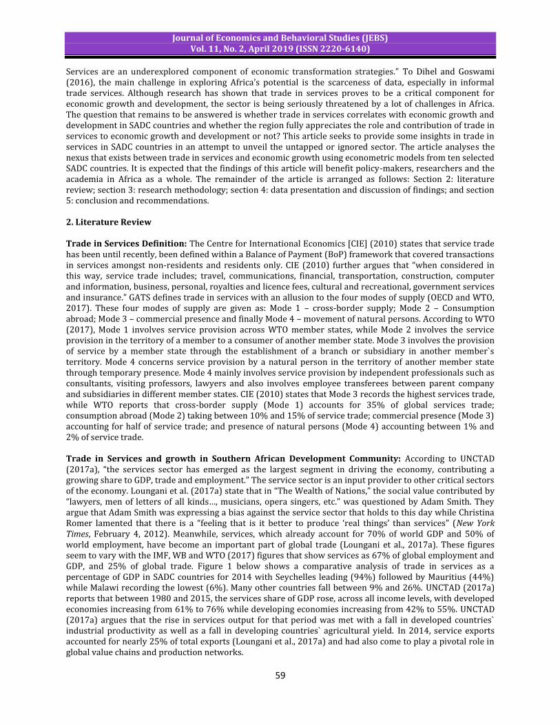
Journal of Economics and Behavioral Studies (JEBS) Vol. 11, No. 2, April 2019 (ISSN 2220-6140)
59
Services are an underexplored component of economic transformation strategies.” To Dihel and Goswami (2016), the main challenge in exploring Africa’s potential is the scarceness of data, especially in informal trade services. Although research has shown that trade in services proves to be a critical component for economic growth and development, the sector is being seriously threatened by a lot of challenges in Africa. The question that remains to be answered is whether trade in services correlates with economic growth and development in SADC countries and whether the region fully appreciates the role and contribution of trade in services to economic growth and development or not? This article seeks to provide some insights in trade in services in SADC countries in an attempt to unveil the untapped or ignored sector. The article analyses the nexus that exists between trade in services and economic growth using econometric models from ten selected SADC countries. It is expected that the findings of this article will benefit policy-makers, researchers and the academia in Africa as a whole. The remainder of the article is arranged as follows: Section 2: literature review; section 3: research methodology; section 4: data presentation and discussion of findings; and section 5: conclusion and recommendations. 2. Literature Review Trade in Services Definition: The Centre for International Economics [CIE] (2010) states that service trade has been until recently, been defined within a Balance of Payment (BoP) framework that covered transactions in services amongst non-residents and residents only. CIE (2010) further argues that “when considered in this way, service trade includes; travel, communications, financial, transportation, construction, computer and information, business, personal, royalties and licence fees, cultural and recreational, government services and insurance.” GATS defines trade in services with an allusion to the four modes of supply (OECD and WTO, 2017). These four modes of supply are given as: Mode 1 – cross-border supply; Mode 2 – Consumption abroad; Mode 3 – commercial presence and finally Mode 4 – movement of natural persons. According to WTO (2017), Mode 1 involves service provision across WTO member states, while Mode 2 involves the service provision in the territory of a member to a consumer of another member state. Mode 3 involves the provision of service by a member state through the establishment of a branch or subsidiary in another member`s territory. Mode 4 concerns service provision by a natural person in the territory of another member state through temporary presence. Mode 4 mainly involves service provision by independent professionals such as consultants, visiting professors, lawyers and also involves employee transferees between parent company and subsidiaries in different member states. CIE (2010) states that Mode 3 records the highest services trade, while WTO reports that cross-border supply (Mode 1) accounts for 35% of global services trade; consumption abroad (Mode 2) taking between 10% and 15% of service trade; commercial presence (Mode 3) accounting for half of service trade; and presence of natural persons (Mode 4) accounting between 1% and 2% of service trade. Trade in Services and growth in Southern African Development Community: According to UNCTAD (2017a), “the services sector has emerged as the largest segment in driving the economy, contributing a growing share to GDP, trade and employment.” The service sector is an input provider to other critical sectors of the economy. Loungani et al. (2017a) state that in “The Wealth of Nations,” the social value contributed by “lawyers, men of letters of all kinds…, musicians, opera singers, etc.” was questioned by Adam Smith. They argue that Adam Smith was expressing a bias against the service sector that holds to this day while Christina Romer lamented that there is a “feeling that is it better to produce ‘real things’ than services” (New York Times, February 4, 2012). Meanwhile, services, which already account for 70% of world GDP and 50% of world employment, have become an important part of global trade (Loungani et al., 2017a). These figures seem to vary with the IMF, WB and WTO (2017) figures that show services as 67% of global employment and GDP, and 25% of global trade. Figure 1 below shows a comparative analysis of trade in services as a percentage of GDP in SADC countries for 2014 with Seychelles leading (94%) followed by Mauritius (44%) while Malawi recording the lowest (6%). Many other countries fall between 9% and 26%. UNCTAD (2017a) reports that between 1980 and 2015, the services share of GDP rose, across all income levels, with developed economies increasing from 61% to 76% while developing economies increasing from 42% to 55%. UNCTAD (2017a) argues that the rise in services output for that period was met with a fall in developed countries` industrial productivity as well as a fall in developing countries` agricultural yield. In 2014, service exports accounted for nearly 25% of total exports (Loungani et al., 2017a) and had also come to play a pivotal role in global value chains and production networks.
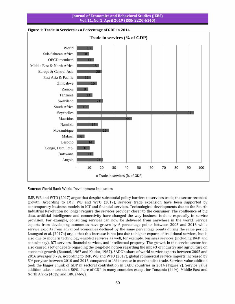
Journal of Economics and Behavioral Studies (JEBS) Vol. 11, No. 2, April 2019 (ISSN 2220-6140)
60
Figure 1: Trade in Services as a Percentage of GDP in 2014
Source: World Bank World Development Indicators IMF, WB and WTO (2017) argue that despite substantial policy barriers to services trade, the sector recorded growth. According to IMF, WB and WTO (2017), services trade expansion have been supported by contemporary business models in ICT and financial services. Technological developments due to the Fourth Industrial Revolution no longer require the services provider closer to the consumer. The confluence of big data, artificial intelligence and connectivity have changed the way business is done especially in service provision. For example, consulting services can now be delivered from anywhere in the world. Service exports from developing economies have grown by 6 percentage points between 2005 and 2016 while service exports from advanced economies declined by the same percentage points during the same period. Loungani et al. (2017a) argue that this increase is not just due to higher exports of traditional services, but is also due to modern technology-enabled services as well, for example, business services (including R&D and consultancy), ICT services, financial services, and intellectual property. The growth in the service sector has also caused a lot of debate regarding the long-held notion regarding the impact of industry and agriculture on economic growth (Baumol, 1967 and Kaldor, 1967). SADC`s share of world service exports between 2005 and 2016 averages 0.7%. According to IMF, WB and WTO (2017), global commercial service imports increased by 5% per year between 2010 and 2015, compared to 1% increase in merchandise trade. Services value addition took the bigger chunk of GDP in sectoral contribution in SADC countries in 2014 (Figure 2). Service value addition takes more than 50% share of GDP in many countries except for Tanzania (44%), Middle East and North Africa (46%) and DRC (46%).
21
13
10
14
6
26
17
44
94
10
21
13
9
16
11
20
18
14
10
13
- 10 20 30 40 50 60 70 80 90 100
Angola
Botswana
Congo, Dem. Rep.
Lesotho
Malawi
Mozambique
Namibia
Mauritius
Seychelles
South Africa
Swaziland
Tanzania
Zambia
Zimbabwe
East Asia & Pacific
Europe & Central Asia
Middle East & North Africa
OECD members
Sub-Saharan Africa
World
Trade in services (% of GDP)
Trade in services (% of GDP)

Journal of Economics and Behavioral Studies (JEBS) Vol. 11, No. 2, April 2019 (ISSN 2220-6140)
61
Figure 2: Sectoral Value Added Share of Gross Domestic Product, 2014 (% of GDP)
Source: World Bank World Development Indicators Services are also predominant in employment with 2010 estimated to have accounted for half (50.9%) of global jobs (figure 3) (Maune, 2017). UNCTAD (2017a) argues that the importance of services is highly evidenced in developed countries where services jobs represent 75% of total employment rather than in developing countries where 44% represents services jobs. Dihel and Goswami (2016) state that, the services sector has become the main employment provider since mid-2000s. This trend has also been witnessed during the 2008–2009 global economic depression. UNCTAD (2017a) further provides that from 2001–2016 the importance of the service sector in the global job market grew taking in developing countries. The service sector has seen more women, that is, 54% employed globally in the sector as of 2013 (figure 4). This is a milestone achievement towards gender parity. Figure 4 shows the share of female employment by sector in 2013 with many countries predominantly services except Zimbabwe, Tanzania, Zambia, Mozambique and Malawi which are predominantly agriculture. The services sector has recorded the highest number of women participation at 41% in developing countries outside the agricultural sector (UNCTAD, 2017a). Figure 3 below shows sectoral employment as a percentage of total employment with services dominating for many SADC countries with the exception of Zimbabwe, Zambia, Tanzania, Mozambique and Malawi where agriculture dominates the sectoral employment share as of 2012.
2
21
5
2
6
31
4
6
25
7
2
2
2
17
6
31
4
7
14
6
18
-
15
11
10
15
-
10
11
15
7
14
11
36
6
15
7
12
59
46
60
72
61
53
74
46
54
61
74
71
68
56
51
44
68
57
57
- 10 20 30 40 50 60 70 80
Botswana
Congo, Dem. Rep.
East Asia & Pacific
Europe & Central Asia
Lesotho
Malawi
Mauritius
Middle East & North Africa
Mozambique
Namibia
OECD members
Seychelles
South Africa
Sub-Saharan Africa
Swaziland
Tanzania
World
Zambia
Zimbabwe
Sectoral value added share of GDP, 2014 (% of GDP)
Services Manufacturing Agriculture
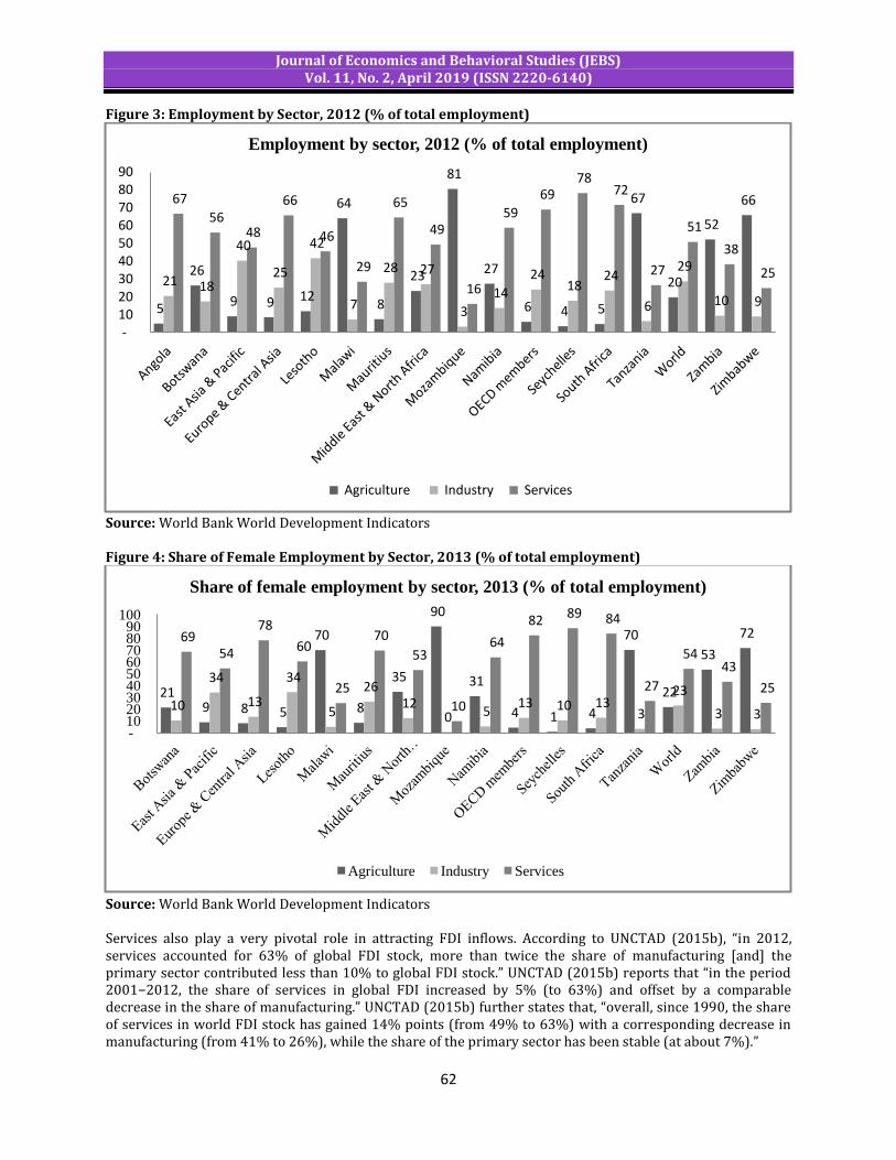
Journal of Economics and Behavioral Studies (JEBS) Vol. 11, No. 2, April 2019 (ISSN 2220-6140)
62
Figure 3: Employment by Sector, 2012 (% of total employment)
Source: World Bank World Development Indicators Figure 4: Share of Female Employment by Sector, 2013 (% of total employment)
Source: World Bank World Development Indicators Services also play a very pivotal role in attracting FDI inflows. According to UNCTAD (2015b), “in 2012, services accounted for 63% of global FDI stock, more than twice the share of manufacturing [and] the primary sector contributed less than 10% to global FDI stock.” UNCTAD (2015b) reports that “in the period 2001−2012, the share of services in global FDI increased by 5% (to 63%) and offset by a comparable decrease in the share of manufacturing.” UNCTAD (2015b) further states that, “overall, since 1990, the share of services in world FDI stock has gained 14% points (from 49% to 63%) with a corresponding decrease in manufacturing (from 41% to 26%), while the share of the primary sector has been stable (at about 7%).”
5
26
9 9 12
64
8
23
81
27
6 4 5
67
20
52
66
21 18
40
25
42
7
28 27
3
14
24 18
24
6
29
10 9
67
56 48
66
46
29
65
49
16
59
69 78
72
27
51
38
25
- 10 20 30 40 50 60 70 80 90
Employment by sector, 2012 (% of total employment)
Agriculture Industry Services
21 9 8 5
70
8
35
90
31
4 1 4
70
22
53
72
10
34
13
34
5
26 12
0 5 13 10 13
3
23
3 3
69 54
78
60
25
70
53
10
64
82 89 84
27
54 43
25
- 10 20 30 40 50 60 70 80 90
100
Share of female employment by sector, 2013 (% of total employment)
Agriculture Industry Services
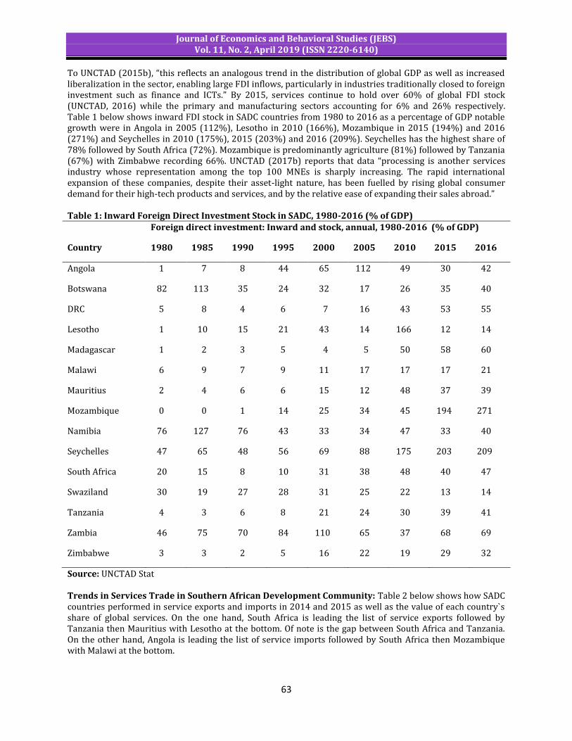
Journal of Economics and Behavioral Studies (JEBS) Vol. 11, No. 2, April 2019 (ISSN 2220-6140)
63
To UNCTAD (2015b), “this reflects an analogous trend in the distribution of global GDP as well as increased liberalization in the sector, enabling large FDI inflows, particularly in industries traditionally closed to foreign investment such as finance and ICTs.” By 2015, services continue to hold over 60% of global FDI stock (UNCTAD, 2016) while the primary and manufacturing sectors accounting for 6% and 26% respectively. Table 1 below shows inward FDI stock in SADC countries from 1980 to 2016 as a percentage of GDP notable growth were in Angola in 2005 (112%), Lesotho in 2010 (166%), Mozambique in 2015 (194%) and 2016 (271%) and Seychelles in 2010 (175%), 2015 (203%) and 2016 (209%). Seychelles has the highest share of 78% followed by South Africa (72%). Mozambique is predominantly agriculture (81%) followed by Tanzania (67%) with Zimbabwe recording 66%. UNCTAD (2017b) reports that data “processing is another services industry whose representation among the top 100 MNEs is sharply increasing. The rapid international expansion of these companies, despite their asset-light nature, has been fuelled by rising global consumer demand for their high-tech products and services, and by the relative ease of expanding their sales abroad.” Table 1: Inward Foreign Direct Investment Stock in SADC, 1980-2016 (% of GDP) Foreign direct investment: Inward and stock, annual, 1980-2016 (% of GDP)
Country 1980 1985 1990 1995 2000 2005 2010 2015 2016
Angola 1 7 8 44 65 112 49 30 42
Botswana 82 113 35 24 32 17 26 35 40
DRC 5 8 4 6 7 16 43 53 55
Lesotho 1 10 15 21 43 14 166 12 14
Madagascar 1 2 3 5 4 5 50 58 60
Malawi 6 9 7 9 11 17 17 17 21
Mauritius 2 4 6 6 15 12 48 37 39
Mozambique 0 0 1 14 25 34 45 194 271
Namibia 76 127 76 43 33 34 47 33 40
Seychelles 47 65 48 56 69 88 175 203 209
South Africa 20 15 8 10 31 38 48 40 47
Swaziland 30 19 27 28 31 25 22 13 14
Tanzania 4 3 6 8 21 24 30 39 41
Zambia 46 75 70 84 110 65 37 68 69
Zimbabwe 3 3 2 5 16 22 19 29 32
Source: UNCTAD Stat Trends in Services Trade in Southern African Development Community: Table 2 below shows how SADC countries performed in service exports and imports in 2014 and 2015 as well as the value of each country`s share of global services. On the one hand, South Africa is leading the list of service exports followed by Tanzania then Mauritius with Lesotho at the bottom. Of note is the gap between South Africa and Tanzania. On the other hand, Angola is leading the list of service imports followed by South Africa then Mozambique with Malawi at the bottom.

Journal of Economics and Behavioral Studies (JEBS) Vol. 11, No. 2, April 2019 (ISSN 2220-6140)
64
Table 2: Southern African Development Community Exports and Imports of Services, 2014 & 2015 (millions of dollars and percentage)
Services exporters
Value of service exports, 2014
Share of global service exports, 2014
Value of service exports, 2015
Share of global service exports, 2015
Services importers
Value of service imports, 2014
Share of global service imports, 2014
Value of service imports, 2015
Share of global service imports, 2015
South Africa 16,837 0.321 15,054 0.304 Angola 24,928 0.492 24,928 0.524 Tanzania 3,396 0.065 3,748 0.076 South Africa 17,042 0.337 15,531 0.326 Mauritius 3,190 0.061 2,843 0.057 Mozambique 3,657 0.072 3,345 0.070 Angola 1,681 0.032 1,256 0.025 DRC 3,082 0.061 2,026 0.043 Botswana 1,352 0.026 1,253 0.025 Tanzania 2,669 0.053 2,685 0.056 Namibia 1,039 0.020 923 0.019 Mauritius 2,498 0.049 2,241 0.047 Zambia 851 0.016 862 0.017 Zimbabwe 1,953 0.039 1,529 0.032 Seychelles 834 0.016 848 0.017 Zambia 1,644 0.032 1,644 0.035 Mozambique 725 0.014 723 0.015 Namibia 1,127 0.022 975 0.020 Zimbabwe 363 0.007 387 0.008 Botswana 774 0.015 628 0.013 DRC 315 0.006 173 0.003 Swaziland 649 0.013 649 0.014 Swaziland 291 0.006 266 0.005 Seychelles 503 0.010 498 0.010 Malawi 109 0.002 116 0.002 Lesotho 334 0.007 315 0.007 Lesotho 30 0.001 46 0.001 Malawi 269 0.005 269 0.006 Total 31,013 0.591 28,497 0.575 Total 61,129 1.207 57,264 1.203
Source: World Bank`s World Development Indicators, NB. The above excludes Madagascar. Developing countries` service exports increasingly strengthened between 2005 and 2016 in comparison with those of the developed countries. Developing countries` service export share increased by 6% from 23% while developed economies declined from 75% to 68% during the same period SADC`s service exports during the same period declined from 0.7% to 0.6%. In 2008 service exports in SADC countries declined to 0.6% from 0.7% in 2007 before rising again to 0.7% in 2010. Table 3 below shows SADC countries` service exports as a percentage of total world exports from 2005 to 2016 with South Africa contributing the highest percentage though less than 1%. However, South Africa share of service exports declined from 0.45% in 2005 to 0.29% in 2016. Mauritius comes second after South Africa with 0.061% in 2005 to 0.06% in 2016. Exports of services have shown resilience compared to exports of goods during the 2009 global economic depression (UNCTAD, 2017a). Table 3: Southern African Development Community Service Exports, 2005-2016 (% of total world)
Service exports, percentage of total world service exports, 2005-2016
Country 2005 2006 2007 2008 2009 2010 2011 2012 2013 2014 2015 2016
Angola 0.007 0.006 0.009 0.008 0.017 0.022 0.017 0.017 0.027 0.033 0.026 0.024
Botswana 0.031 0.026 0.024 0.016 0.023 0.025 0.028 0.027 0.026 0.026 0.026 0.027
DRC 0.013 0.014 0.011 0.021 0.018 0.010 0.017 0.006 0.006 0.006 0.004 -
Lesotho 0.001 0.001 0.001 0.001 0.001 0.001 0.001 0.001 0.001 0.001 0.001 0.001
Madagascar 0.019 0.022 0.028 0.032 0.024 0.026 0.027 0.029 0.026 0.025 0.022 0.020
Malawi 0.003 0.002 0.002 0.002 0.002 0.002 0.002 0.002 0.002 0.002 0.002 0.002
Mauritius 0.061 0.056 0.062 0.063 0.062 0.069 0.074 0.075 0.058 0.062 0.058 0.059
Mozambique 0.013 0.013 0.013 0.014 0.017 0.006 0.008 0.017 0.013 0.014 0.015 0.009
Namibia 0.016 0.018 0.017 0.014 0.018 0.017 0.017 0.024 0.019 0.020 0.019 0.014
Seychelles 0.014 0.014 0.013 0.012 0.012 0.011 0.011 0.015 0.017 0.016 0.017 0.018
South Africa 0.446 0.436 0.415 0.348 0.368 0.410 0.394 0.389 0.349 0.327 0.310 0.294
Swaziland 0.008 0.009 0.014 0.006 0.006 0.007 0.007 0.005 0.005 0.006 0.005 0.003
Tanzania 0.048 0.051 0.052 0.050 0.052 0.052 0.052 0.062 0.066 0.066 0.077 0.076
Zambia 0.021 0.019 0.019 0.015 0.015 0.015 0.015 0.022 0.016 0.017 0.018 0.018
Zimbabwe 0.014 0.011 0.008 0.006 0.007 0.007 0.008 0.008 0.007 0.007 0.008 -
Source: UNCTAD Stat
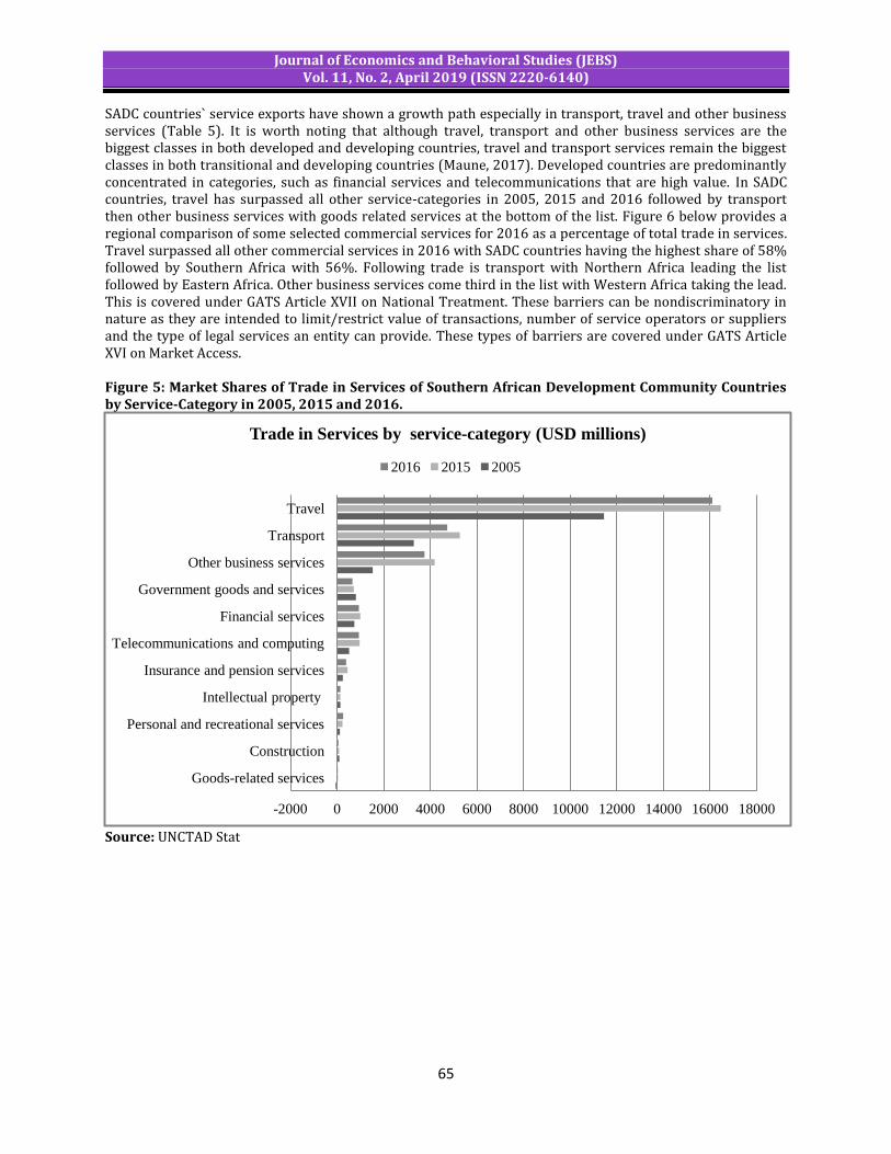
Journal of Economics and Behavioral Studies (JEBS) Vol. 11, No. 2, April 2019 (ISSN 2220-6140)
65
SADC countries` service exports have shown a growth path especially in transport, travel and other business services (Table 5). It is worth noting that although travel, transport and other business services are the biggest classes in both developed and developing countries, travel and transport services remain the biggest classes in both transitional and developing countries (Maune, 2017). Developed countries are predominantly concentrated in categories, such as financial services and telecommunications that are high value. In SADC countries, travel has surpassed all other service-categories in 2005, 2015 and 2016 followed by transport then other business services with goods related services at the bottom of the list. Figure 6 below provides a regional comparison of some selected commercial services for 2016 as a percentage of total trade in services. Travel surpassed all other commercial services in 2016 with SADC countries having the highest share of 58% followed by Southern Africa with 56%. Following trade is transport with Northern Africa leading the list followed by Eastern Africa. Other business services come third in the list with Western Africa taking the lead. This is covered under GATS Article XVII on National Treatment. These barriers can be nondiscriminatory in nature as they are intended to limit/restrict value of transactions, number of service operators or suppliers and the type of legal services an entity can provide. These types of barriers are covered under GATS Article XVI on Market Access. Figure 5: Market Shares of Trade in Services of Southern African Development Community Countries by Service-Category in 2005, 2015 and 2016.
Source: UNCTAD Stat
-2000 0 2000 4000 6000 8000 10000 12000 14000 16000 18000
Goods-related services
Construction
Personal and recreational services
Intellectual property
Insurance and pension services
Telecommunications and computing
Financial services
Government goods and services
Other business services
Transport
Travel
Trade in Services by service-category (USD millions)
2016 2015 2005

Journal of Economics and Behavioral Studies (JEBS) Vol. 11, No. 2, April 2019 (ISSN 2220-6140)
66
Figure 6: Exports of Selected Commercial Services by Region, 2016 (% of total trade in services)
Source: UNCTAD Stat Services Trade Policy Landscape in Southern African Development Community: In general services are inputs providers to all exports related industries. For this to succeed, it requires services trade policies that adequately facilitate the smooth flow of trade globally without unnecessary barriers and restrictions. According to OECD and WTO (2017), “services trade barriers are embedded in the legal and regulatory frameworks and these barriers mainly involve government measures discriminating foreign services or suppliers.” The two barriers, that is, national treatment and market access largely determine a country`s service market competitiveness. Regulators can intentionally play around with the two to encourage contestability and market competition in a country. OECD and WTO (2017) list some of the forms of service trade barriers and these include; foreign investment discretionary screening, license caps, restrictions in the movement of natural persons, monopolies, foreign equity limits and discriminatory subsidies or licensing requirements. Literature has shown that barriers to services trade are high in many SADC countries and these restrictions have negatively affected foreign investment inflows and cross-border trade. The situation is further worsened by high cross-border trade costs. Although trade restrictions are meant to protect domestic industries, the resultant effects are not that as intended as these protected domestic service providers’ ends up charging exorbitant prices thereby harming the consumers in the process due to high production costs and low competition. This situation will cause smuggling of cheap foreign services and products that will result in the collapse of the domestic companies due to stiff competition. This has been the case in Zimbabwe after the introduction of Statutory Instrument 64. Local companies that were protected by government through restrictions in foreign imports went on to inflate prices and creating artificial shortages to the detriment of innocent consumers at the end. According to the Services Trade Restrictiveness by the World Bank, there are five categories that are defined by the restrictiveness level linked to a score. These scores are scaled from 0 to 100, with 100 the worst outcome and 0 being the best outcome. The five categories are:
0 - Completely open. 25 - Virtually open (with minor restrictions). 50 - Major restrictions. 75 - Virtually closed (with limited opportunities to enter and operate) and 100 - Completely closed.
- 10 20 30 40 50 60 70
Africa
Eastern Africa
Middle Africa
Northern Africa
Southern Africa
Western Africa
LDCs
SSA
SADC
Exports of selected commercial services by region, 2016 (% of total
trade in services)
Government goods and services
Personal and recreational services
Other business services
Telecommunications & computing
Intellectual property
Financial services
Insurance and pension services
Construction
Travel
Transport
Goods-related services
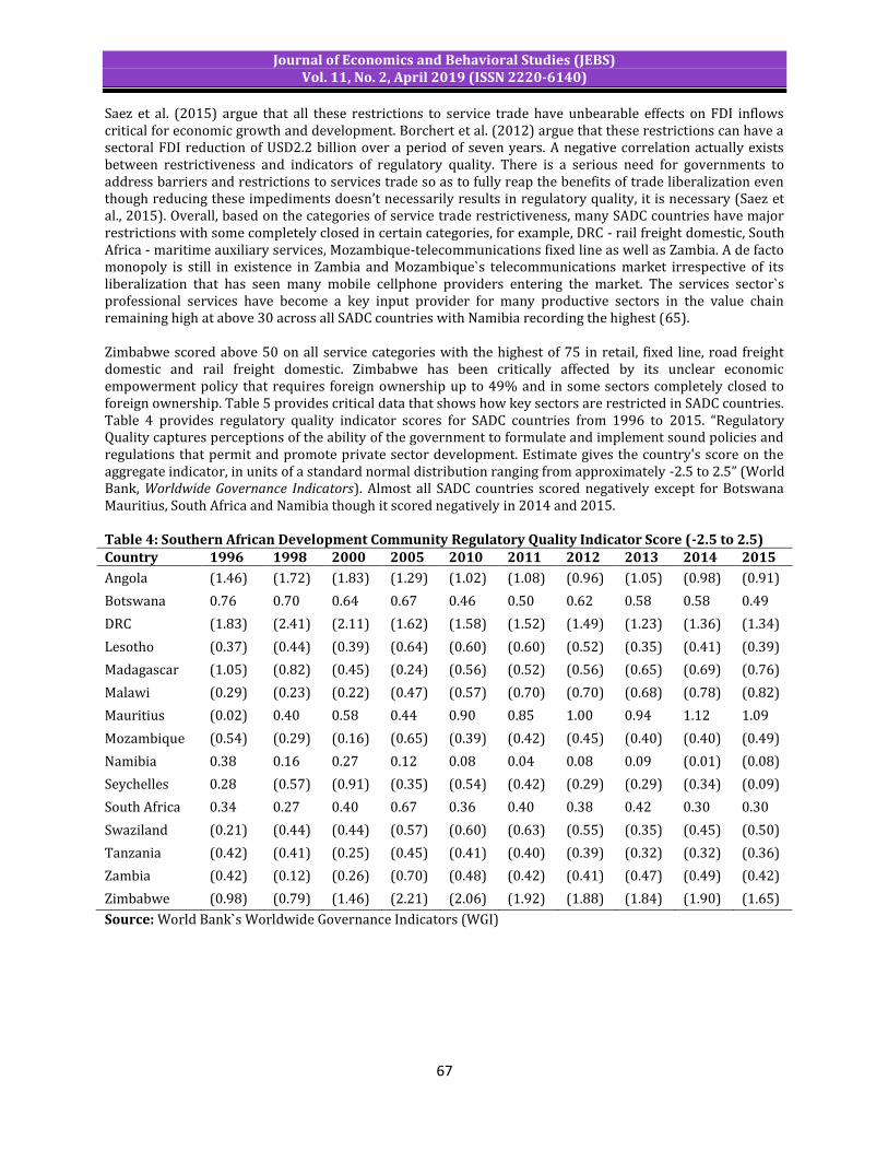
Journal of Economics and Behavioral Studies (JEBS) Vol. 11, No. 2, April 2019 (ISSN 2220-6140)
67
Saez et al. (2015) argue that all these restrictions to service trade have unbearable effects on FDI inflows critical for economic growth and development. Borchert et al. (2012) argue that these restrictions can have a sectoral FDI reduction of USD2.2 billion over a period of seven years. A negative correlation actually exists between restrictiveness and indicators of regulatory quality. There is a serious need for governments to address barriers and restrictions to services trade so as to fully reap the benefits of trade liberalization even though reducing these impediments doesn’t necessarily results in regulatory quality, it is necessary (Saez et al., 2015). Overall, based on the categories of service trade restrictiveness, many SADC countries have major restrictions with some completely closed in certain categories, for example, DRC - rail freight domestic, South Africa - maritime auxiliary services, Mozambique-telecommunications fixed line as well as Zambia. A de facto monopoly is still in existence in Zambia and Mozambique`s telecommunications market irrespective of its liberalization that has seen many mobile cellphone providers entering the market. The services sector`s professional services have become a key input provider for many productive sectors in the value chain remaining high at above 30 across all SADC countries with Namibia recording the highest (65). Zimbabwe scored above 50 on all service categories with the highest of 75 in retail, fixed line, road freight domestic and rail freight domestic. Zimbabwe has been critically affected by its unclear economic empowerment policy that requires foreign ownership up to 49% and in some sectors completely closed to foreign ownership. Table 5 provides critical data that shows how key sectors are restricted in SADC countries. Table 4 provides regulatory quality indicator scores for SADC countries from 1996 to 2015. “Regulatory Quality captures perceptions of the ability of the government to formulate and implement sound policies and regulations that permit and promote private sector development. Estimate gives the country's score on the aggregate indicator, in units of a standard normal distribution ranging from approximately -2.5 to 2.5” (World Bank, Worldwide Governance Indicators). Almost all SADC countries scored negatively except for Botswana Mauritius, South Africa and Namibia though it scored negatively in 2014 and 2015. Table 4: Southern African Development Community Regulatory Quality Indicator Score (-2.5 to 2.5) Country 1996 1998 2000 2005 2010 2011 2012 2013 2014 2015
Angola (1.46) (1.72) (1.83) (1.29) (1.02) (1.08) (0.96) (1.05) (0.98) (0.91)
Botswana 0.76 0.70 0.64 0.67 0.46 0.50 0.62 0.58 0.58 0.49
DRC (1.83) (2.41) (2.11) (1.62) (1.58) (1.52) (1.49) (1.23) (1.36) (1.34)
Lesotho (0.37) (0.44) (0.39) (0.64) (0.60) (0.60) (0.52) (0.35) (0.41) (0.39)
Madagascar (1.05) (0.82) (0.45) (0.24) (0.56) (0.52) (0.56) (0.65) (0.69) (0.76)
Malawi (0.29) (0.23) (0.22) (0.47) (0.57) (0.70) (0.70) (0.68) (0.78) (0.82)
Mauritius (0.02) 0.40 0.58 0.44 0.90 0.85 1.00 0.94 1.12 1.09
Mozambique (0.54) (0.29) (0.16) (0.65) (0.39) (0.42) (0.45) (0.40) (0.40) (0.49)
Namibia 0.38 0.16 0.27 0.12 0.08 0.04 0.08 0.09 (0.01) (0.08)
Seychelles 0.28 (0.57) (0.91) (0.35) (0.54) (0.42) (0.29) (0.29) (0.34) (0.09)
South Africa 0.34 0.27 0.40 0.67 0.36 0.40 0.38 0.42 0.30 0.30
Swaziland (0.21) (0.44) (0.44) (0.57) (0.60) (0.63) (0.55) (0.35) (0.45) (0.50)
Tanzania (0.42) (0.41) (0.25) (0.45) (0.41) (0.40) (0.39) (0.32) (0.32) (0.36)
Zambia (0.42) (0.12) (0.26) (0.70) (0.48) (0.42) (0.41) (0.47) (0.49) (0.42)
Zimbabwe (0.98) (0.79) (1.46) (2.21) (2.06) (1.92) (1.88) (1.84) (1.90) (1.65)
Source: World Bank`s Worldwide Governance Indicators (WGI)

Journal of Economics and Behavioral Studies (JEBS) Vol. 11, No. 2, April 2019 (ISSN 2220-6140)
68
Table 5: Southern African Development Community`s Services Trade Restrictiveness Index, 2015 (score 0 to 100)
Category BWA DRC LSO MDG MWI MUS MOZ NAM ZAF TZA ZMB ZWE
Overall 38 52 27 19 34 17 19 37 35 31 21 64
Financial 30 40 0 31 35 9 17 27 20 23 8 56
Telecommunications 50 50 25 25 50 0 75 50 25 25 75 63
Fixed-line 50 50 25 25 50 0 100 25 25 25 100 75
Mobile 50 50 25 25 50 0 50 75 25 25 50 50
Retail 25 75 50 0 25 0 0 25 25 25 0 75
Transportation 55 55 23 6 32 31 6 30 41 29 10 68 Air Passenger International 68 50 60 35 50 53 35 29 36 60 35 50 Maritime Shipping International 33 0 0 0 0 8 8 0 Maritime Auxiliary Services 50 0 0 75 0 25 100 50
Road Freight Domestic 50 50 0 0 25 0 0 50 25 0 0 75
Rail Freight Domestic 50 100 0 25 0 25 25 50 0 75
Professional 47 36 37 38 38 42 30 65 62 52 44 60
Accounting & Auditing 45 10 20 40 30 25 28 45 40 40 40 55
Legal 48 53 48 36 43 53 32 78 77 59 47 63
Source: World Bank`s Services Trade Restrictiveness Database Empirical Evidence: Empirically, a growing number of studies have examined the nexus between trade and economic growth. Exports-growth nexus has been a subject of extensive debate since the 1960s. It is surprising that there is no clear consensus between the export-led growth hypothesis (ELG) and growth led-exports hypothesis (GLE) even though early cross-section studies preferred the earlier, it should probably be the latter instead of the past. However, the findings from these studies have been a mixed bag across methodologies and countries. Lee and Huang (2002) cite ELG as a key factor in promoting economic growth. Rigobon and Rodrik (2005) study that found a negative though significant influence of trade on income levels. Chia (2016) argues that many researchers have done ELG using diverse econometric techniques. In the analysis Chia (2016) found that causal relationships vary with, (1) period of study, (2) econometric methods used, (3) variable treatment, and (4) inclusion of other associated variables in the estimated equation. Chia (2016) states “that positive productivity effects estimated by ELG hypothesis don’t necessarily occur in developing countries.” This is due to heavy dependence on exports of primary commodities in many developing economies. Chia (2016) further examined the validity of ELG in three African countries from 1985 to 2014 using FMOLS, DOLS, panel unit-root tests and co-integration approaches. The findings show non-stationarity of variables in level and stationarity in the first difference. A long-run nexus was presented by the panel co-integration estimation between the variables. The impact of ELG was, however, positive and highly significant statistically. According to Medina-Smith (2001), “ELG postulates that export expansion is one of the main determinants of growth. It holds that the overall growth of countries can be generated not only by increasing the amounts of labour and capital within the economy but also by expanding exports. According to its advocates, exports can perform as an ‘engine of growth’”. According to World Bank (1993), “phenomenal growth rates achieved by the south-east Asian countries between 1970s and 1990s following successful implementation of the ELG strategy provide evidence in support of the superiority of ELG strategy.” “Although a substantial part of the earlier studies found evidence of a correlation between exports and growth which was used to support the ELG, this tends to hold only for cross-section studies” (Medina-Smith, 2001). Medina-Smith (2001) further argues that “the recent evidence on time series, which makes extensive use of cointegration techniques, casts doubts on the

Journal of Economics and Behavioral Studies (JEBS) Vol. 11, No. 2, April 2019 (ISSN 2220-6140)
69
positive effects of exports on growth in the long run, and is thus not as conclusive as it was previously thought to be.” The study by Pazim (2009) on ELG was coherent with studies by Fosu (1990) and Ukpolo (1994) that were done in the African context. In his study Kónya (2004), investigates the possibility of ELG and GLE by testing for Granger causality between the logarithms of real exports and real GDP in twenty-five OECD countries. Kónya (2004) found “no causality between exports and growth in Luxembourg and in the Netherlands, exports cause growth (ECG) in Iceland, growth causes exports (GCE) in Canada, Japan and Korea, and there is two-way causality between exports and growth in Sweden and in the UK.” Although with less certainty, Kónya (2004) concludes “that there is no causality in Denmark, France, Greece, Hungary and Norway, ECG in Australia, Austria and Ireland, and GCE in Finland, Portugal and the USA.” However, in the case of Belgium, Italy, Mexico, New Zealand, Spain and Switzerland, Kónya (2004) `s results are contentious to make a simple choice. In his study in 35 countries from 1860 to 1963, Goldsmith (1969) finds “a rough correlation between financial development (as measured by total domestic credit over GDP) and growth. Goldsmith further uses the ratio of the value of financial intermediary assets to GNP to gauge financial performance and enters it in regression with economic growth as the dependent variable.” Since then, Jung (1986) and Odedokun (1991) have found that “the depth and growth of financial markets had a significant effect on growth in developing countries.” Dash and Parida (2013) examine the linkages between inward FDI, services trade and economic output using co-integration and VECM causality test. The empirical findings confirm the long-run relationship among these variables. Causality results indicate the presence of bi-directional causal relationship between FDI and economic output as well as between service exports and economic output. The results by Dash and Parida (2013) also bring out feedback relationship between service exports and FDI, reconfirming the presence of complementary relationship between the two. Sang-Chul (2017) examined, “using country-level panel data and System Generalized Method of Moments technique, the nexus between trade openness and growth. A sample of 25 Asian economies during the period 2005 to 2013 was selected. The estimation results showed that services trade openness had a negative and statistically significant effect on GDP, while trade openness had a positive and statistically significant effect on GDP for the Asian countries. The results are indicative of negative strong growth effects of openness in services trade in high-income countries, while weak in the low-income countries.” El Khoury and Savvides (2006) “examine the relationship between openness in services trade and economic growth via the threshold regression model to test for a differential impact between low- and high-income countries. Results confirm the existence of a two-regime split.” El Khoury and Savvides (2006) conclude that the greater openness in services trade is associated with higher growth. A study by Tekin (2012) of 27 African LDCs resulted in no causality linking three variables, that is, trade openness, foreign aid and GDP per capita. A study by Ajmia et al. (2013) tested causality between exports and GDP in South Africa. They used both linear and non-linear tests and the findings showed a cointegrating nexus among the two, and unidirectional causality from GDP to exports. In their conclusion, they argued that exports have a positive influence on GDP through increased incomes, employment and the development of technology. In an analysis by Asfaw (2014), trade openness was found to be a stimulant for both economic growth and investment. The study focused on the effect of trade liberalization on growth in 47 sub-Saharan African countries. A study by Fenira (2015) shows a weak nexus between trade openness and GDP. Sakyi, Villaverde, and Maza (2015) provide “evidence of a positive bi-directional causal relationship between trade and economic growth for a sample of 115 developing countries.” Were (2015) finds that “trade exerts a positive and significant effect on economic growth rate in developed and developing countries, but its effect is not significant for least developed countries which largely include African countries?” Trejos and Barboza (2015) provide robust empirical evidence that trade openness is not the main engine of the Asian economic growth “miracle.” A study by Brueckner and Lederman (2015) found that trade openness increases growth in the short and long run. Their study employed an instrumental variable approach on 41 sub-Saharan African countries. In an investigation by Musila and Yiheyis (2015) in Kenya, trade openness was found to have a positive effect on investment ratio and not on growth. In a more related study in South Africa, Polat et al. (2015) find that trade openness impedes growth. Sakyi, Commodore, and Opoku (2015) investigated the long-run impact of FDI and trade openness on economic growth in Ghana
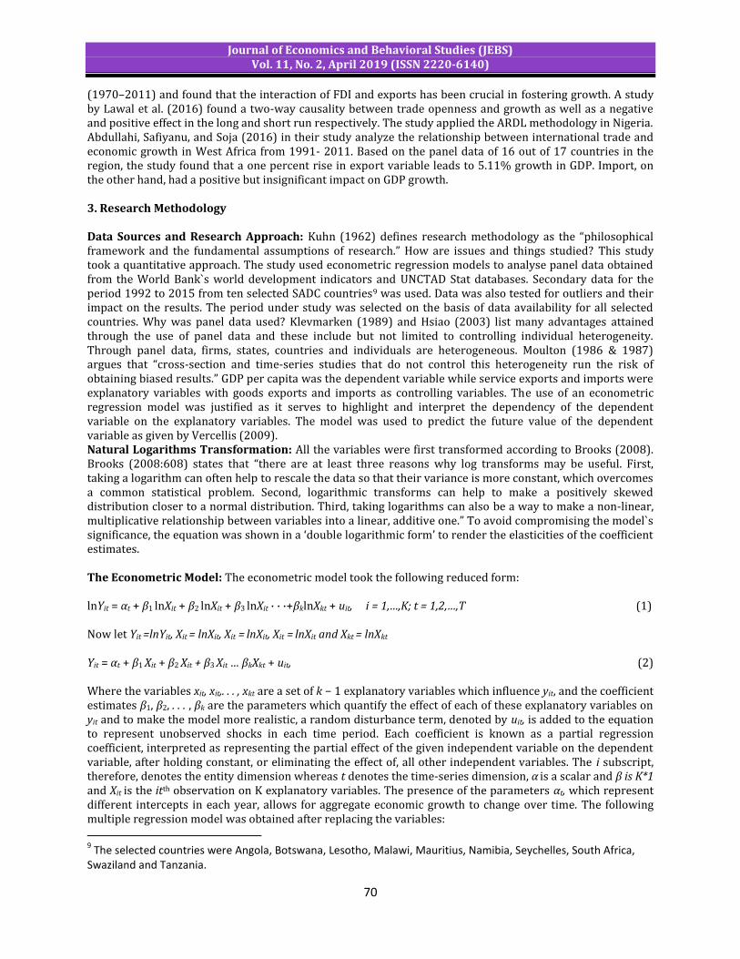
Journal of Economics and Behavioral Studies (JEBS) Vol. 11, No. 2, April 2019 (ISSN 2220-6140)
70
(1970–2011) and found that the interaction of FDI and exports has been crucial in fostering growth. A study by Lawal et al. (2016) found a two-way causality between trade openness and growth as well as a negative and positive effect in the long and short run respectively. The study applied the ARDL methodology in Nigeria. Abdullahi, Safiyanu, and Soja (2016) in their study analyze the relationship between international trade and economic growth in West Africa from 1991- 2011. Based on the panel data of 16 out of 17 countries in the region, the study found that a one percent rise in export variable leads to 5.11% growth in GDP. Import, on the other hand, had a positive but insignificant impact on GDP growth. 3. Research Methodology Data Sources and Research Approach: Kuhn (1962) defines research methodology as the “philosophical framework and the fundamental assumptions of research.” How are issues and things studied? This study took a quantitative approach. The study used econometric regression models to analyse panel data obtained from the World Bank`s world development indicators and UNCTAD Stat databases. Secondary data for the period 1992 to 2015 from ten selected SADC countries9 was used. Data was also tested for outliers and their impact on the results. The period under study was selected on the basis of data availability for all selected countries. Why was panel data used? Klevmarken (1989) and Hsiao (2003) list many advantages attained through the use of panel data and these include but not limited to controlling individual heterogeneity. Through panel data, firms, states, countries and individuals are heterogeneous. Moulton (1986 & 1987) argues that “cross-section and time-series studies that do not control this heterogeneity run the risk of obtaining biased results.” GDP per capita was the dependent variable while service exports and imports were explanatory variables with goods exports and imports as controlling variables. The use of an econometric regression model was justified as it serves to highlight and interpret the dependency of the dependent variable on the explanatory variables. The model was used to predict the future value of the dependent variable as given by Vercellis (2009). Natural Logarithms Transformation: All the variables were first transformed according to Brooks (2008). Brooks (2008:608) states that “there are at least three reasons why log transforms may be useful. First, taking a logarithm can often help to rescale the data so that their variance is more constant, which overcomes a common statistical problem. Second, logarithmic transforms can help to make a positively skewed distribution closer to a normal distribution. Third, taking logarithms can also be a way to make a non-linear, multiplicative relationship between variables into a linear, additive one.” To avoid compromising the model`s significance, the equation was shown in a ‘double logarithmic form’ to render the elasticities of the coefficient estimates. The Econometric Model: The econometric model took the following reduced form: lnYit = αt + β1 lnXit + β2 lnXit + β3 lnXit · · ·+βklnXkt + uit, i = 1,…,K; t = 1,2,…,T (1) Now let Yit =lnYit, Xit = lnXit, Xit = lnXit, Xit = lnXit and Xkt = lnXkt Yit = αt + β1 Xit + β2 Xit + β3 Xit … βkXkt + uit, (2) Where the variables xit, xit,. . . , xkt are a set of k − 1 explanatory variables which influence yit, and the coefficient estimates β1, β2, . . . , βk are the parameters which quantify the effect of each of these explanatory variables on yit and to make the model more realistic, a random disturbance term, denoted by uit, is added to the equation to represent unobserved shocks in each time period. Each coefficient is known as a partial regression coefficient, interpreted as representing the partial effect of the given independent variable on the dependent variable, after holding constant, or eliminating the effect of, all other independent variables. The i subscript, therefore, denotes the entity dimension whereas t denotes the time-series dimension, α is a scalar and β is K*1 and Xit is the itth observation on K explanatory variables. The presence of the parameters αt, which represent different intercepts in each year, allows for aggregate economic growth to change over time. The following multiple regression model was obtained after replacing the variables:
9 The selected countries were Angola, Botswana, Lesotho, Malawi, Mauritius, Namibia, Seychelles, South Africa,
Swaziland and Tanzania.

Journal of Economics and Behavioral Studies (JEBS) Vol. 11, No. 2, April 2019 (ISSN 2220-6140)
71
gdpit = αt + β1 servicesexpit + β2 servicesimpit + β3 goodsexpit + β4 goodsimpit + uit (3) 4. Data Analysis and Interpretation Panel Unit-Root Tests: Panel unit root test was conducted to perform a variety of tests for unit roots (or stationarity) in panel datasets using the Fisher-type (Choi, 2001) and Hadri (2000) Lagrange multiplier (LM) tests on each of the variables for the entire period of 1992 to 2015. The results are presented in Table 6 below. The results reveal overwhelming evidence against the null hypothesis of all panels containing unit roots with the exception of goods exports under the Fisher-type unit root test based on Philips-Perron. This means there are no unit roots in the panels under the given test conditions. The null hypothesis of a unit root is rejected in favour of the stationary alternative under the ADF because the test statistic is more negative than the critical value. The variables are therefore stationary, hence no need for co-integration analysis. Table 6: Panel Unit Root Test of Each Variable
Variable
Fisher-type Augmented Dickey-Fuller test
Hadri LM test Fisher-type PPerron test
z(t) p-value z(t) z(t) p-value Gdp -5.4282 0.0000 8.1936 -1.4934 0.0677 Services exp -6.4476 0.0000 5.7222 -5.4064 0.0000 Services imp -5.6089 0.0000 9.4256 -3.1391 0.0008 Goods exp -4.4453 0.0000 18.5945 1.8749 0.9696 Goods imp -3.5390 0.0002 22.7829 -1.8370 0.0331 Source: Author`s compilation from STATA/SE 12.0 Correlation Matrix: This matrix shows a positive nexus amongst the variables, that is, dependent and explanatory though the relationship is weak except for service exports (Table 7). The correlation doesn’t infer causativeness. Keho (2017) argues that “a positive relationship between trade variables and GDP fits well with the trade-led growth hypothesis, the growth-led trade hypothesis or a two-way causality amongst trade variables and GDP.” Table 7: Correlation Matrix, Influence of Trade on Economic Growth in Selected SADC Countries
Source: Extract from STATA/SE 12.0 Main Regression Model Results: A multiple regression was run using panel data to predict the impact of trade on economic growth in SADC countries. GDP per capita was the dependent variable with service exports and imports being the explanatory variables, while goods exports and imports were the controlling variables. The Stat result below (table 8) summarizes the regression coefficients estimates and statistics. The ANOVA table is shown on the upper left part together with mean sum squares (MS), degrees of freedom (DF) and sum squares (SS). Out of the SS of 356.78, 144.70 is explained by the model while 212.08 remains unaccounted, that is, residual. The SS explained by the model is the SS after taking out the means as a result of the effect of the regression constant. Also reported is the total DF of 234 (i.e. 235 less 1 being mean removal), from which 4 is explained by the model while 230 is the residual. The MS results from dividing SS by DF. F-statistic and R2 are summarized on the upper right part of table 8. F-statistic is that is derived from the upper left part of the ANOVA table. The ratio is thus, F = (Model SS/dfModel) / (Residual SS/dfResidual). Therefore, F = 36.17 / 0.922 =
lnservice~mp 0.2932 0.9279 0.8968 0.7483 1.0000
lnservice~xp 0.5626 0.7034 0.7696 1.0000
lngoodsimp 0.2972 0.9518 1.0000
lngoodsexp 0.2997 1.0000
lngdp 1.0000
lngdp lngoo~xp lngoo~mp lnser~xp lnser~mp
(obs=235)
. correlate lngdp lngoodsexp lngoodsimp lnservicesexp lnservicesimp
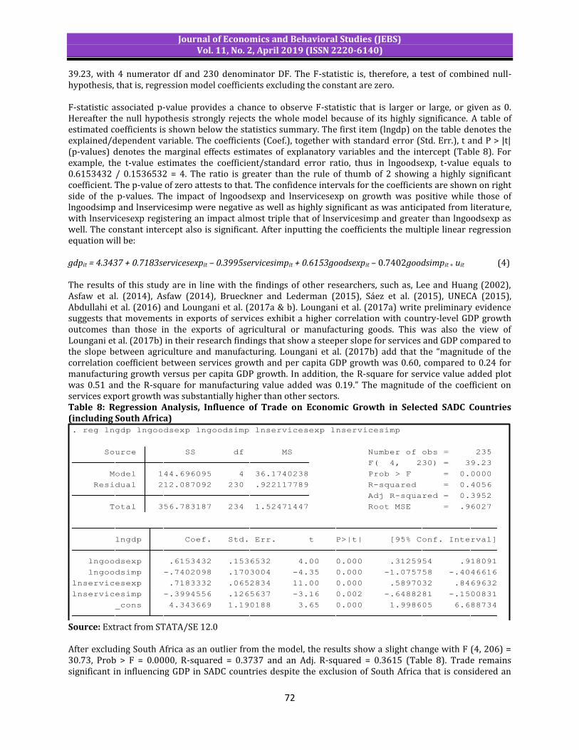
Journal of Economics and Behavioral Studies (JEBS) Vol. 11, No. 2, April 2019 (ISSN 2220-6140)
72
39.23, with 4 numerator df and 230 denominator DF. The F-statistic is, therefore, a test of combined null-hypothesis, that is, regression model coefficients excluding the constant are zero. F-statistic associated p-value provides a chance to observe F-statistic that is larger or large, or given as 0. Hereafter the null hypothesis strongly rejects the whole model because of its highly significance. A table of estimated coefficients is shown below the statistics summary. The first item (lngdp) on the table denotes the explained/dependent variable. The coefficients (Coef.), together with standard error (Std. Err.), t and P > |t| (p-values) denotes the marginal effects estimates of explanatory variables and the intercept (Table 8). For example, the t-value estimates the coefficient/standard error ratio, thus in lngoodsexp, t-value equals to 0.6153432 / 0.1536532 = 4. The ratio is greater than the rule of thumb of 2 showing a highly significant coefficient. The p-value of zero attests to that. The confidence intervals for the coefficients are shown on right side of the p-values. The impact of lngoodsexp and lnservicesexp on growth was positive while those of lngoodsimp and lnservicesimp were negative as well as highly significant as was anticipated from literature, with lnservicesexp registering an impact almost triple that of lnservicesimp and greater than lngoodsexp as well. The constant intercept also is significant. After inputting the coefficients the multiple linear regression equation will be: gdpit = 4.3437 + 0.7183servicesexpit – 0.3995servicesimpit + 0.6153goodsexpit – 0.7402goodsimpit + uit (4) The results of this study are in line with the findings of other researchers, such as, Lee and Huang (2002), Asfaw et al. (2014), Asfaw (2014), Brueckner and Lederman (2015), Sáez et al. (2015), UNECA (2015), Abdullahi et al. (2016) and Loungani et al. (2017a & b). Loungani et al. (2017a) write preliminary evidence suggests that movements in exports of services exhibit a higher correlation with country-level GDP growth outcomes than those in the exports of agricultural or manufacturing goods. This was also the view of Loungani et al. (2017b) in their research findings that show a steeper slope for services and GDP compared to the slope between agriculture and manufacturing. Loungani et al. (2017b) add that the “magnitude of the correlation coefficient between services growth and per capita GDP growth was 0.60, compared to 0.24 for manufacturing growth versus per capita GDP growth. In addition, the R-square for service value added plot was 0.51 and the R-square for manufacturing value added was 0.19.” The magnitude of the coefficient on services export growth was substantially higher than other sectors. Table 8: Regression Analysis, Influence of Trade on Economic Growth in Selected SADC Countries (including South Africa)
Source: Extract from STATA/SE 12.0 After excluding South Africa as an outlier from the model, the results show a slight change with F (4, 206) = 30.73, Prob > F = 0.0000, R-squared = 0.3737 and an Adj. R-squared = 0.3615 (Table 8). Trade remains significant in influencing GDP in SADC countries despite the exclusion of South Africa that is considered an
_cons 4.343669 1.190188 3.65 0.000 1.998605 6.688734
lnservicesimp -.3994556 .1265637 -3.16 0.002 -.6488281 -.1500831
lnservicesexp .7183332 .0652834 11.00 0.000 .5897032 .8469632
lngoodsimp -.7402098 .1703004 -4.35 0.000 -1.075758 -.4046616
lngoodsexp .6153432 .1536532 4.00 0.000 .3125954 .918091
lngdp Coef. Std. Err. t P>|t| [95% Conf. Interval]
Total 356.783187 234 1.52471447 Root MSE = .96027
Adj R-squared = 0.3952
Residual 212.087092 230 .922117789 R-squared = 0.4056
Model 144.696095 4 36.1740238 Prob > F = 0.0000
F( 4, 230) = 39.23
Source SS df MS Number of obs = 235
. reg lngdp lngoodsexp lngoodsimp lnservicesexp lnservicesimp
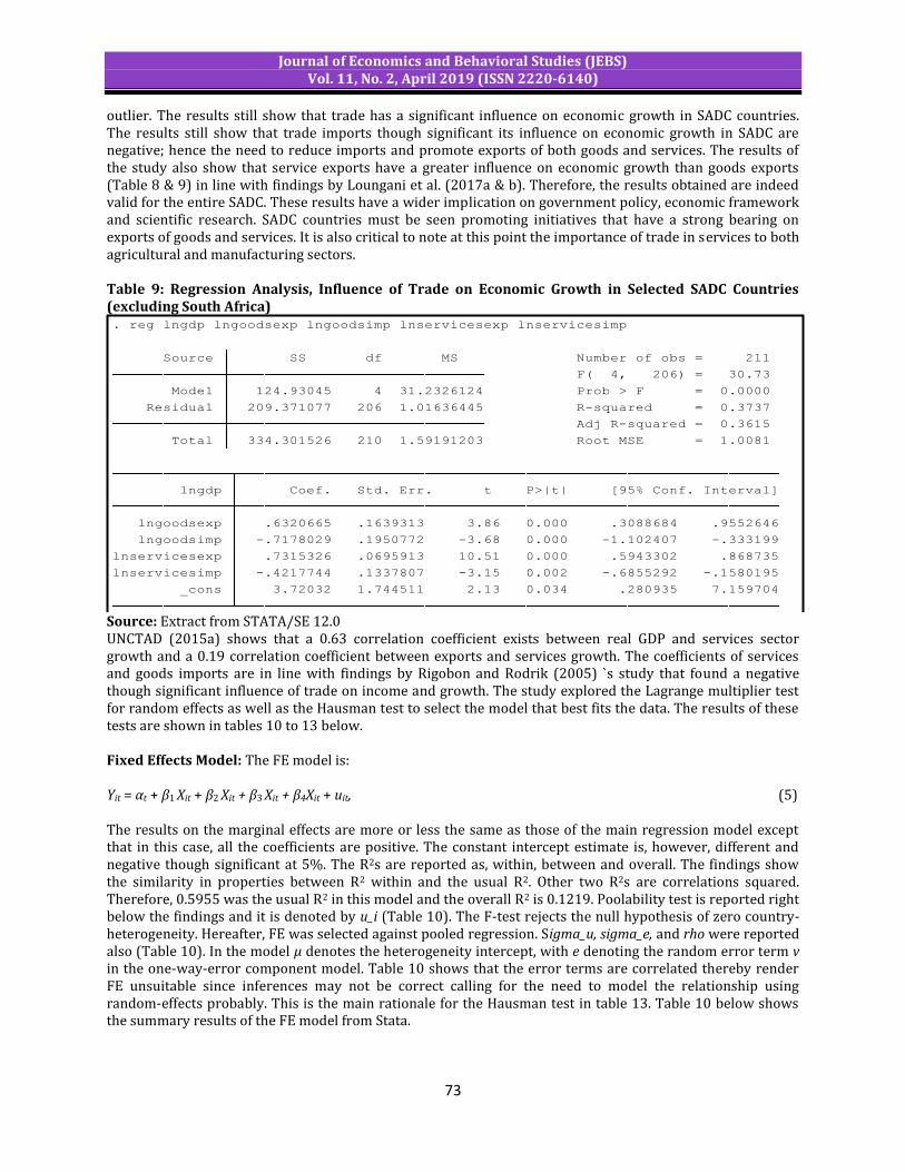
Journal of Economics and Behavioral Studies (JEBS) Vol. 11, No. 2, April 2019 (ISSN 2220-6140)
73
outlier. The results still show that trade has a significant influence on economic growth in SADC countries. The results still show that trade imports though significant its influence on economic growth in SADC are negative; hence the need to reduce imports and promote exports of both goods and services. The results of the study also show that service exports have a greater influence on economic growth than goods exports (Table 8 & 9) in line with findings by Loungani et al. (2017a & b). Therefore, the results obtained are indeed valid for the entire SADC. These results have a wider implication on government policy, economic framework and scientific research. SADC countries must be seen promoting initiatives that have a strong bearing on exports of goods and services. It is also critical to note at this point the importance of trade in services to both agricultural and manufacturing sectors. Table 9: Regression Analysis, Influence of Trade on Economic Growth in Selected SADC Countries (excluding South Africa)
Source: Extract from STATA/SE 12.0 UNCTAD (2015a) shows that a 0.63 correlation coefficient exists between real GDP and services sector growth and a 0.19 correlation coefficient between exports and services growth. The coefficients of services and goods imports are in line with findings by Rigobon and Rodrik (2005) `s study that found a negative though significant influence of trade on income and growth. The study explored the Lagrange multiplier test for random effects as well as the Hausman test to select the model that best fits the data. The results of these tests are shown in tables 10 to 13 below. Fixed Effects Model: The FE model is: Yit = αt + β1 Xit + β2 Xit + β3 Xit + β4Xit + uit, (5) The results on the marginal effects are more or less the same as those of the main regression model except that in this case, all the coefficients are positive. The constant intercept estimate is, however, different and negative though significant at 5%. The R2s are reported as, within, between and overall. The findings show the similarity in properties between R2 within and the usual R2. Other two R2s are correlations squared. Therefore, 0.5955 was the usual R2 in this model and the overall R2 is 0.1219. Poolability test is reported right below the findings and it is denoted by u_i (Table 10). The F-test rejects the null hypothesis of zero country-heterogeneity. Hereafter, FE was selected against pooled regression. Sigma_u, sigma_e, and rho were reported also (Table 10). In the model μ denotes the heterogeneity intercept, with e denoting the random error term v in the one-way-error component model. Table 10 shows that the error terms are correlated thereby render FE unsuitable since inferences may not be correct calling for the need to model the relationship using random-effects probably. This is the main rationale for the Hausman test in table 13. Table 10 below shows the summary results of the FE model from Stata.
_cons 3.72032 1.744511 2.13 0.034 .280935 7.159704
lnservicesimp -.4217744 .1337807 -3.15 0.002 -.6855292 -.1580195
lnservicesexp .7315326 .0695913 10.51 0.000 .5943302 .868735
lngoodsimp -.7178029 .1950772 -3.68 0.000 -1.102407 -.333199
lngoodsexp .6320665 .1639313 3.86 0.000 .3088684 .9552646
lngdp Coef. Std. Err. t P>|t| [95% Conf. Interval]
Total 334.301526 210 1.59191203 Root MSE = 1.0081
Adj R-squared = 0.3615
Residual 209.371077 206 1.01636445 R-squared = 0.3737
Model 124.93045 4 31.2326124 Prob > F = 0.0000
F( 4, 206) = 30.73
Source SS df MS Number of obs = 211
. reg lngdp lngoodsexp lngoodsimp lnservicesexp lnservicesimp
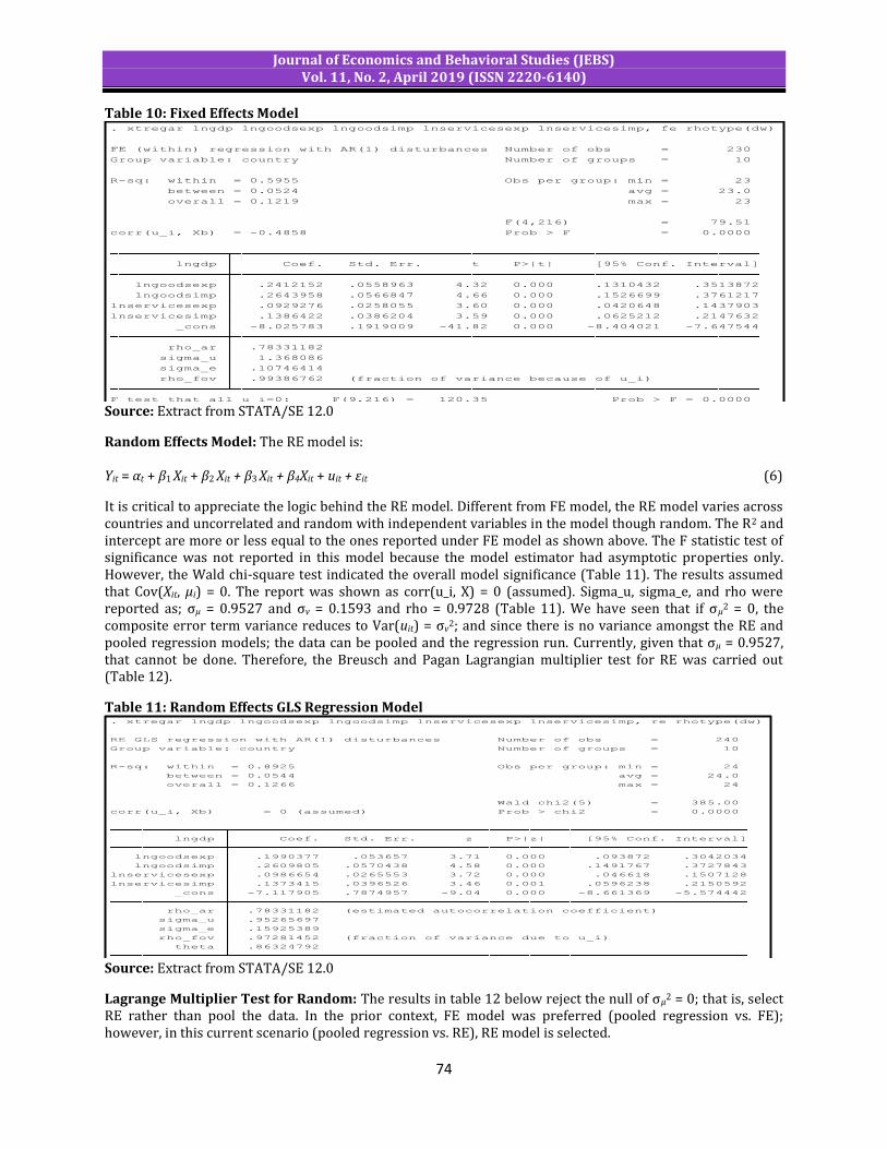
Journal of Economics and Behavioral Studies (JEBS) Vol. 11, No. 2, April 2019 (ISSN 2220-6140)
74
Table 10: Fixed Effects Model
Source: Extract from STATA/SE 12.0
Random Effects Model: The RE model is: Yit = αt + β1 Xit + β2 Xit + β3 Xit + β4Xit + uit + εit (6)
It is critical to appreciate the logic behind the RE model. Different from FE model, the RE model varies across countries and uncorrelated and random with independent variables in the model though random. The R2 and intercept are more or less equal to the ones reported under FE model as shown above. The F statistic test of significance was not reported in this model because the model estimator had asymptotic properties only. However, the Wald chi-square test indicated the overall model significance (Table 11). The results assumed that Cov(Xit, μi) = 0. The report was shown as corr(u_i, X) = 0 (assumed). Sigma_u, sigma_e, and rho were reported as; σμ = 0.9527 and σv = 0.1593 and rho = 0.9728 (Table 11). We have seen that if σμ2 = 0, the composite error term variance reduces to Var(uit) = σv
2; and since there is no variance amongst the RE and pooled regression models; the data can be pooled and the regression run. Currently, given that σμ = 0.9527, that cannot be done. Therefore, the Breusch and Pagan Lagrangian multiplier test for RE was carried out (Table 12).
Table 11: Random Effects GLS Regression Model
Source: Extract from STATA/SE 12.0
Lagrange Multiplier Test for Random: The results in table 12 below reject the null of σμ2 = 0; that is, select RE rather than pool the data. In the prior context, FE model was preferred (pooled regression vs. FE); however, in this current scenario (pooled regression vs. RE), RE model is selected.
F test that all u_i=0: F(9,216) = 120.35 Prob > F = 0.0000
rho_fov .99386762 (fraction of variance because of u_i)
sigma_e .10746414
sigma_u 1.368086
rho_ar .78331182
_cons -8.025783 .1919009 -41.82 0.000 -8.404021 -7.647544
lnservicesimp .1386422 .0386204 3.59 0.000 .0625212 .2147632
lnservicesexp .0929276 .0258055 3.60 0.000 .0420648 .1437903
lngoodsimp .2643958 .0566847 4.66 0.000 .1526699 .3761217
lngoodsexp .2412152 .0558963 4.32 0.000 .1310432 .3513872
lngdp Coef. Std. Err. t P>|t| [95% Conf. Interval]
corr(u_i, Xb) = -0.4858 Prob > F = 0.0000
F(4,216) = 79.51
overall = 0.1219 max = 23
between = 0.0524 avg = 23.0
R-sq: within = 0.5955 Obs per group: min = 23
Group variable: country Number of groups = 10
FE (within) regression with AR(1) disturbances Number of obs = 230
. xtregar lngdp lngoodsexp lngoodsimp lnservicesexp lnservicesimp, fe rhotype(dw)
theta .86324792
rho_fov .97281452 (fraction of variance due to u_i)
sigma_e .15925389
sigma_u .95265697
rho_ar .78331182 (estimated autocorrelation coefficient)
_cons -7.117905 .7874957 -9.04 0.000 -8.661369 -5.574442
lnservicesimp .1373415 .0396526 3.46 0.001 .0596238 .2150592
lnservicesexp .0986654 .0265553 3.72 0.000 .046618 .1507128
lngoodsimp .2609805 .0570438 4.58 0.000 .1491767 .3727843
lngoodsexp .1990377 .053657 3.71 0.000 .093872 .3042034
lngdp Coef. Std. Err. z P>|z| [95% Conf. Interval]
corr(u_i, Xb) = 0 (assumed) Prob > chi2 = 0.0000
Wald chi2(5) = 385.00
overall = 0.1266 max = 24
between = 0.0544 avg = 24.0
R-sq: within = 0.8925 Obs per group: min = 24
Group variable: country Number of groups = 10
RE GLS regression with AR(1) disturbances Number of obs = 240
. xtregar lngdp lngoodsexp lngoodsimp lnservicesexp lnservicesimp, re rhotype(dw)
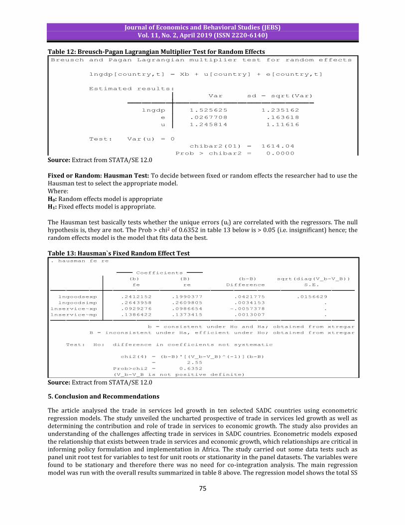
Journal of Economics and Behavioral Studies (JEBS) Vol. 11, No. 2, April 2019 (ISSN 2220-6140)
75
Table 12: Breusch-Pagan Lagrangian Multiplier Test for Random Effects
Source: Extract from STATA/SE 12.0 Fixed or Random: Hausman Test: To decide between fixed or random effects the researcher had to use the Hausman test to select the appropriate model. Where: H0: Random effects model is appropriate H1: Fixed effects model is appropriate. The Hausman test basically tests whether the unique errors (ui) are correlated with the regressors. The null hypothesis is, they are not. The Prob > chi2 of 0.6352 in table 13 below is > 0.05 (i.e. insignificant) hence; the random effects model is the model that fits data the best. Table 13: Hausman`s Fixed Random Effect Test
Source: Extract from STATA/SE 12.0
5. Conclusion and Recommendations
The article analysed the trade in services led growth in ten selected SADC countries using econometric regression models. The study unveiled the uncharted prospective of trade in services led growth as well as determining the contribution and role of trade in services to economic growth. The study also provides an understanding of the challenges affecting trade in services in SADC countries. Econometric models exposed the relationship that exists between trade in services and economic growth, which relationships are critical in informing policy formulation and implementation in Africa. The study carried out some data tests such as panel unit root test for variables to test for unit roots or stationarity in the panel datasets. The variables were found to be stationary and therefore there was no need for co-integration analysis. The main regression model was run with the overall results summarized in table 8 above. The regression model shows the total SS
Prob > chibar2 = 0.0000
chibar2(01) = 1614.04
Test: Var(u) = 0
u 1.245814 1.11616
e .0267708 .163618
lngdp 1.525625 1.235162
Var sd = sqrt(Var)
Estimated results:
lngdp[country,t] = Xb + u[country] + e[country,t]
Breusch and Pagan Lagrangian multiplier test for random effects
(V_b-V_B is not positive definite)
Prob>chi2 = 0.6352
= 2.55
chi2(4) = (b-B)'[(V_b-V_B)^(-1)](b-B)
Test: Ho: difference in coefficients not systematic
B = inconsistent under Ha, efficient under Ho; obtained from xtregar
b = consistent under Ho and Ha; obtained from xtregar
lnservice~mp .1386422 .1373415 .0013007 .
lnservice~xp .0929276 .0986654 -.0057378 .
lngoodsimp .2643958 .2609805 .0034153 .
lngoodsexp .2412152 .1990377 .0421775 .0156629
fe re Difference S.E.
(b) (B) (b-B) sqrt(diag(V_b-V_B))
Coefficients
. hausman fe re

Journal of Economics and Behavioral Studies (JEBS) Vol. 11, No. 2, April 2019 (ISSN 2220-6140)
76
of 356.78, of which 144.70 is explained by the model while 212.08 remains unaccountable (residual). Also reported is the total DF of 234 (i.e. 235 less 1 being mean removal), from which 4 is explained by the model while 230 is the residual. The model strongly rejects the null hypothesis thereby rendering it highly significant as a whole. The constant intercept is significant as well. The study further explored the Lagrange multiplier test for random effects as well as the Hausman test to select the model that best fits the data with the results summarized in table 10 up to table 13 above. Table 10 rendered FE unsuitable due to the correlation of error terms resulting in RE being used to model the relationship as shown by the Hausman test in table 13. The Hausman test was used to help the researcher to select the appropriate model that fits the data the best. It is critical at this point to note the positive and significant contribution shown by the coefficient, services exports in table 8 and 9. This is actually in line with what literature has shown with regards to the services sector being a critical component of economic growth and development. This notion has, however, challenged long-held theories of economic development the world over. Prior researches and theories had found the typical steps out of poverty to be increased agricultural productivity followed by growth in the manufacturing sector. However, the past years have seen the world experiencing a different trajectory in economic growth and development with manufacturing sector instead of growing as theory might have anticipated, remained stagnant while agriculture`s share of GDP declined. However, services have been on an increase as measured by its share of total employment, exports and GDP. Trade in services has been argued to be the driver of value addition and provider of critical inputs to boost other economic activities. Services have become predominant in employment with 2010 estimated to have accounted for half (50.9%) of global jobs. The share of female employment by sector in 2013 was predominantly services except for Zimbabwe, Tanzania, Zambia, Mozambique and Malawi which are predominantly agriculture. Although empirically the results show the significance of service exports on economic growth in SADC as a whole, it is of critical importance. To identify service categories critical for each country so that each country can concentrate on those categories where she has comparative and competitive advantage rather than focusing on the whole services sector. Figure 5 shows that a lot has been done or is being realized from travel, transport and other business services categories in that order. However, there is a lot of potential lying in other categories such as financial services, telecommunications & computing, insurance & pension services, intellectual property and construction. Figure 6 shows exports of selected commercial services by region and travel ranks high in SADC, SSA, LDCs, Southern Africa, Middle Africa, Eastern Africa and Africa as a whole. There are quite a number of benefits that have accrued due to the developments in services trade although it`s potential is being hampered by a number of policy restrictions. Governments need to seriously consider remove services trade restrictions and avoid over-regulating the sector to fully realize it`s potential. Given the technological developments in this Fourth Industrial Revolution, the services sector is becoming a critical sector in the development of economies. More researches need to be carried out to have better knowledge and understanding of trade in services, its potential and challenges to economic development in Africa. The impact of cyber security risk needs to be taken seriously as it poses greater threats to trade in services across the globe. This risk can, however, be taken as an opportunity by innovators through coming up with solutions that counter the threats. Policy-makers and government need to clearly define their service agenda and strategy in their policies. A three-legged approach that involves government, private sector and academia is critical in formulating and designing trade-in service policies.
References
Abdullahi, A. O., Safiyanu, S. S. & Soja, T. (2016). International Trade and Economic Growth: An Empirical Analysis of West Africa, Journal of Economics and Finance, 7(2), 12-15.
Ajmi, A. N., Ayeb, G. C., Balcilarc, M. & Guptad, R. (2013). Causality between Exports and Economic Growth in South Africa: Evidence from Linear and Nonlinear Tests, Working Paper Series, University of Pretoria Department of Economics.
Asfaw, H. A. (2014). Trade policy and economic growth in Sub- Saharan Africa: A panel data approach,” American Journal of Trade and Policy, 1, 94–101.
Borchert, I., Gootiiz, B. & Mattoo, A. (2012). Policy Barriers to International Trade in Services: Evidence from a New Database, Policy Research Working Paper No. 6109, Washington, DC: World Bank.

Journal of Economics and Behavioral Studies (JEBS) Vol. 11, No. 2, April 2019 (ISSN 2220-6140)
77
Brooks, C. (2008). Introductory Econometrics for Finance, 2nd ed., New York: Cambridge University Press. Brueckner, M. & Lederman, D. (2015). Trade openness and economic growth: Panel data evidence from Sub-
Saharan Africa, Economica, 82, 1302–1323. Centre for International Economics. (2010). Quantifying the benefits of services trade liberalization, Report
prepared for Department of Foreign Affairs and Trade, Canberra: Australia. www.TheCIE.com.au. Chia, Y. E. (2016). Export-Led Growth Hypothesis: Empirical Evidence from Selected sub-Saharan African
Countries, Procedia Economics and Finance, 35, 232–240. Choi, I. (2001). Unit root tests for panel data, Journal of International Money and Finance, 20, 249–272. Dash, R. K. & Parida, P. C. (2013). FDI, services trade and economic growth in India: empirical evidence on
causal links, Empir Econ, 45, 217–238. Dihel, N. & Goswami, A. G. (2016). From Hair Stylists and Teachers to Accountants and Doctors: The
Unexplored Potential of Trade in Services in Africa, Washington, D.C.: World Bank Group. El Khoury, A. C. & Savvides, A. (2006). Openness in services trade and economic growth, Economics Letters,
92, 277-283. Fenira, M. (2015). Trade openness and growth in developing countries: An analysis of the relationship after
comparing trade indicators, Asian Economic and Financial Review, 5, 468–482. Financial Sector in Economic Growth: Time Series Evidence from LDCs, Journal of Development Economics,
50(1), 119-46. Fosu, A. K. (1990). Exports and economic growth: the African Case, World Development, 18(6), 831-35. Goldsmith, R. W. (1969). Financial Structure and Development, New Haven, CT: Yale U. Press. Hadri, K. (2000). Testing for stationarity in heterogeneous panel data, Econometrics Journal, 3, 148–161. Hoekman, B. & Shepherd, B. (2017). Services Productivity, Trade Policy and Manufacturing Exports," World
Economy, 40(3), 499-516. Hoekman, B. & te Velde, D. W. (eds.) (2017). Trade in services and economic transformation: A new
development policy priority, London: ODI. (http://set.odi.org). Hsiao, C. (2003). Analysis of Panel Data, Cambridge University Press, Cambridge. International Monetary Fund, World Bank, and World Trade Organization. (2017). Making Trade an Engine of
Growth for All: The Case for Trade and for Policies to Facilitate Adjustment, Geneva: World Trade Organisation.
Jung, W. S. (1986). Financial Development and Economic Growth: International Evidence, Economic Development and Cultural Change, 34(2), 336-346.
Keho, Y. (2017). The impact of trade openness on economic growth: The case of Cote d’Ivoire, Cogent Economics & Finance, 5, 1-14.
Klevmarken, N. A. (1989). Panel studies: What can we learn from them? Introduction, European Economic Review, 33, 523–529.
Kónya, L. (2004). Export-led growth, growth-driven export, both or none? Granger causality analysis on OECD countries, Applied Econometrics and International Development, AEEADE, 4(1), 73-94.
Kowalski, P., Lopez Gonzalez, J., Ragoussis, A. & Ugarte, C. (2015). Participation of Developing Countries in Global Value Chains: Implications for Trade and Trade-Related Policies, OECD Trade Policy Papers, No. 179, Paris: OECD Publishing.
Kuhn, T. S. (1962). The Structure of Scientific Revolutions, Chicago, University of Chicago Press. Lawal, A. I., Nwanji, T. I., Asaleye, A. & Ahmed, V. (2016). Economic growth, financial development and trade
openness in Nigeria: An application of the ARDL bound testing approach, Cogent Economics and Finance, 4, 1–15.
Lee, C. & Huang, D. (2002). Human Capital Distribution, Growth and Trade, Bulletin of Economic Research and John Wiley & Sons Ltd, 66(1), 1467-8586.
Loungani, P., Mishra, S., Papageorgiou, C. & Wang, K. (2017a). The Future Wealth of Nations: World Trade in Services, IMF Research Bulletin, 18(1), 4-7.
Loungani, P., Mishra, S., Papageorgiou, C. & Wang, K. (2017b). World Trade in Services: Evidence from a New Dataset, World Trade in Services, 1-41.
Maune, A. (2017). Trade in services and economic benefits in Africa: Evidence from Zimbabwe. Paper presented at the International Conference on Financial Services, Western Cape, South Africa.
Medina-Smith, E. J. (2001). Is the export-led growth hypothesis valid for developing countries? A case study of Costa Rica, Policy issues in International Trade and Commodities Study series No. 7: Geneva, United Nations.
Journal of Economics and Behavioral Studies (JEBS) Vol. 11, No. 2, April 2019 (ISSN 2220-6140)
78
Moulton, B. R. (1986). Random group effects and the precision of regression estimates, Journal of Econometrics, 32, 385–397.
Moulton, B. R. (1987). Diagnostics for group effects in regression analysis, Journal of Business and Economic Statistics, V5, 275–282.
Musila, J. W. & Yiheyis, Z. (2015). The impact of trade openness on growth: The case of Kenya, Journal of Policy Modeling, 37, 342–354.
Odedokun, M. O. (1996). Alternative Econometric Approaches for Analysing the Role. OECD. & WTO. (2015). Aid for Trade at a Glance 2015: Reducing Trade Costs for Inclusive, Sustainable
Growth, Geneva: World Trade Organisation. OECD. & WTO. (2017). Aid for Trade at a glance 2017: Promoting Trade, Inclusiveness and Connectivity for
Sustainable Development,” Geneva: World Trade Organisation. Pazim, K. H. (2009). Panel data analysis of export-led growth hypothesis in BIMP-EAGA Countries: University
Library of Munich, Germany. Polat, A., Shahbaz, M., Rehman, I. U. & Satti, S. L. (2015). Revisiting linkages between financial development,
trade openness and economic growth in South Africa: Fresh evidence from combined cointegration test, Quality and Quantity, 49, 785–803.
Rigobon, R. & Rodrik, D. (2005). Rule of law, democracy, openness, and income: Estimating the interrelationships, The Economics of Transition, 13, 533–564.
Sáez, S., Mckenna, M. & Hoffman, B. (2015). Valuing Trade in Services in Africa, The Africa Competitiveness Report 2015, Washington, D.C.: World Bank Group.
Sakyi, D., Commodore, R. & Opoku, E. E. (2015). Foreign Direct Investment, Trade Openness and Economic Growth in Ghana: An Empirical Investigation, Journal of African Business, 16(1-2), 1-15.
Sakyi, D., Villaverde, J. & Maza, A. (2015). Trade openness, income levels, and economic growth: The case of developing countries, 1970–2009, The Journal of International Trade & Economic Development, 24, 860– 882.
Sang-Chul, Y. (2017). Trade Openness and Economic Growth: A Panel data Analysis of Asian Countries,
무역보험연구 제18권 제3호, 9, 1-19.
Tekin, R. B. (2012). Development aid, openness to trade and economic growth in least developed countries: Bootstrap panel granger causality analysis, Procedia-Social and Behavioral Sciences, 62, 716–721.
Trejos, S. & Barboza, B. (2015). Dynamic estimation of the relationship between trade openness and output growth in Asia, J. Asian Econ. 36, 110–125.
Ukpolo, V. (1994). Export Composition and growth of selected low-income African countries: evidence from time-series data, Applied Economics, 26, 445-449.
UNCTAD. (2015a). Unlocking the potential of Africa’s services trade for Growth and development, Economic Development in Africa Report, UN, NY.
UNCTAD. (2015b). World Investment Report: Reforming International Investment Governance, Geneva: United Nations.
UNCTAD. (2016). World Investment Report: Investor Nationality: Policy Challenges, Geneva: United Nations. UNCTAD. (2017a). The role of the services economy and trade in structural transformation and inclusive
development, Geneva: United Nations. UNCTAD. (2017b). World Investment Report: Investment and the Digital Economy, Geneva: United Nations. United Nations Economic Commission for Africa. (2015). Economic Report on Africa 2015: Industrializing
through trade, United Nations, Addis Ababa, Ethiopia. USITC (United States International Trade Commission). (2015). Factors contributing to the rapid growth of
Mauritius’ services economy, USITC Executive Briefing on Trade, July. Vercellis, C. (2009). Business Intelligence: Data Mining and Optimization for Decision making, United
Kingdom: Wiley & Sons Ltd. Were, M. (2015). Differential effects of trade on economic growth and investment: A cross-country empirical
investigation, Journal of African Trade, 2, 71–85. World Bank. (1993). The East Asian Miracle: Economic Growth and Public Policy: New York, Oxford
University Press.

Journal of Economics and Behavioral Studies (JEBS) Vol. 11, No. 2, April 2019 (ISSN 2220-6140)
79
Enhanced Customer Interactions through Customer-Centric Technology within a Call Centre
Devina Oodith University of KwaZulu-Natal (Westville Campus), Durban, South Africa
[email protected] Abstract: Customer call centres have become a critical form of service delivery for many organisations hence technological innovations serve as a critical point of contact between the organisation and its customers and can assist in raising the stakes in businesses in terms of customer service delivery (Burgess & Connell, 2004). According to the 2017 Global Customer Experience Benchmarking Report technology has been the number one enabler to positively enhance customer service experience in the last 5 years (Business Tech, 2017). Customers have become so empowered that they expect to have flexibility to contact a business however they choose; either via a telephone, email or Facebook. The key to ensuring satisfaction though is system’s efficiency and ease of use. This study was undertaken in EThekwini (Durban), South Africa and was directed within a Public Sector service environment comprising of four major call centres employing a total of 240 call centre agents. Using simple random sampling, 220 customers were drawn from all consumers subscribing to e-billing in EThekwini (Durban). Data for the customer sample was collected using a precoded, self-developed questionnaire whose psychometric properties were statistically determined. Data was analyzed using descriptive and inferential statistics. The results specify that in terms of customers’ perceptions of the influence of technology, on call centre effectiveness the majority of the customers found it challenging to use the technology and to understand the self-help options that were provided to them by the call centre. There were problems encountered with logging in customer queries and complaints and most customers were dissatisfied with their overall customer experience. Based on the results of the study recommendations have been made to manage the interactions between the customers and call centre’s more proficiently and powerfully. Keywords: Systems efficiency, ease of use, clarity and understanding of technology.
1. Introduction In the absence of the traditional servicescape and while waiting on the phone for their call to be answered, customers only have access to their audio senses (Whiting & Donthu, 2006). During this time most of the customers are likely to experience anger and frustration coupled with boredom as they are compelled to deal with inadequate menu options, delays in waiting for agents, coping with aggravating music while waiting, fragmented human contact by numerous call centre agents; usually asking for basic information to be repeated; which often leads to failed calls, and results in repeat journeys through this tedious cycle due to failed service encounters (Beirre et al., 2004, p100). The objectives and importance of this paper is to assess the effectiveness of customer interactions within the call centre through customer-centric technology. In particular it explores the extent to which the systems that are available to assist customers are efficient in handling queries and complaints (systems efficiency); whether these systems are simple to use and understand by the customers that have to interface and navigate through them (ease of use) and attempts to address whether the instructions and menu options presented to customers are clear and concise (clarity and understanding). The telephone call centres are becoming increasingly popular in the service sector. Thus low-cost telecommunications and computer software have been implemented across the finance, banking, insurance and customer support sectors and towards customer call centres as the primary mode of service delivery (Ellis & Taylor, 2006). More recently there have been increases in internet only financial service providers in a bid to benefit from lower costs that have been incurred than from the traditional pressures of the call centre with the additional overheads across the firm; and the heightened dependency on call centre agents (Dixon, 2002; Piercy & Rich, 2008). Systems Efficiency: Information systems and information technology (IS/IT) has been recognised as a core competitive and strategic competency for many organisations (Bendoly et al., 2009; Cheng et al., 2011). Even though IS/IT plays a pivotal role within the organisation the actual effectiveness of its utilisation is important to deliberate upon. Many service managers today are employing several strategies which focus on delivering integrated services using real-time applications to customers (Geum et al., 2011). In this regard service
Journal of Economics and Behavioral Studies (JEBS) Vol. 11, No. 2, April 2019 (ISSN 2220-6140)
80
delivery utilises a range of offerings which include competencies such as automation, zero touch, self-managed, agile and real-time customer offerings (Ojiako, 2012). Some scholars such as Venkatesh and Agarwal (2006) believe that IS/IT is essential to the delivery of the customer experience. According to Ojiako (2012), the interactions between customers and service providers are also being impacted by advances in IS/IT which enables standardisation and the potential for cost reduction for the service provider. Service providers are now being driven to provide innovative services and more self-managed customer interactions (Gelderman et al., 2011; Lin & Hsieh, 2011). The last decade has seen greater adoption of mobile technology and self-service technologies (SST’s) in order to create cost savings (Lavin & Maynard, 2001). However recent studies have revealed great frustrations and difficulties being experienced by customers with the SST models being implemented by businesses (Reinders et al., 2008; Robertson & Shaw, 2009). The type of service support needed by the customer has been found to be critical in terms of the service encounter. Lu et al. (2009) and Mattila et al. (2011) found that the desire to use SST’s is influenced by the customer’s sense of personal capacity to engage with the SST. Hence the greater the perceived risk of the transaction the greater the likelihood that the customer will seek the assistance of a call centre agent rather than engage with technology. Makarem et al. (2009) found that a good IS/IT-enabled service process did not have as much positive impact as the traditional good “human contact” in terms of the perception of overall customer satisfaction. Ease of Use: There are many prospects for self-service suggesting that provider motivation and customer benefits can grow this mode of business (Hsieh, 2005). Customers will be more accommodating of this mode as a result of increased opportunity for customization, accuracy, convenience and speed. According to Fitzsimmons & Fitzsimmons (2006), due to the increase in the cost of human labour, inroads have been created for self-service technology (SST). The advent of this technology will see an end to low wage, unskilled, non-value-added service jobs. The firm has the advantage of serving more customers with fewer resources; thus, reducing costs while the customer has the ability to customise a product or service for personal use at a time convenient for the customer (Borck, 2004; Hsieh, 2005; Malgeri, 2007; Ruyter et al., 2000). Hsieh (2005) identified three primary goals that firms may strive towards by entering the self-service arena. They firstly strive to enhance the customer’s service by assisting customers with queries without tying up the firm’s human resources. Indeed if this is executed correctly, it has the potential to save the firm money (Malgeri, 2007). Secondly, the firm can enable direct transactions such as customer orders and exchanges without any direct interaction with an employee. Finally, through online educational guidance customers can train themselves to use the site. Hsieh (2005) identified the following factors that can affect the adoption and use of self-service technology:
Quality of products Services offered by the firm Cost of the product Presentation of services Design of self-service technology The self-service technology’s ability for service recovery Promotion of self-service technology The way the firm manages and prevents self-service technology failure Alternative uses for the same service (competitors) The firm’s ability to keep the self-service technology updated and to improve it continuously
Girman, Keusch & Kmec (2009) undertook a study on the use of vending machines within a University campus environment and attempted to track the number of faults that were experienced by the users of these machines. They found that although no official complaints were lodged with the service provider, regular inspections carried out by maintenance crew detected faults with some of the machines. They also investigated the use of pay phones that worked with coins and prepaid cards and again discovered that these phones did have defects present, although no official complaints were received. Girman, Keusch & Kmec (2009) highlighted the importance of periodic checks as long as complaint rates were low, in order to
Journal of Economics and Behavioral Studies (JEBS) Vol. 11, No. 2, April 2019 (ISSN 2220-6140)
81
maintain a level of service quality when firms embrace self-service technology. The service provider must conduct these checks because minor failures may not always be reported but can dissuade first-time users from using self-service technology in the future. Internet Services: E-business came about as a result of a convergence of several technologies. A website can serve altered purposes for diverse businesses. According to Metters et al. (2006), reports indicate a decline in customer satisfaction with most services. Customers grow irate with automated phone systems and a host of new terminology encountered during internet encounters. As a result, many customers encounter long waiting times with e-mail queries and misunderstandings arise as a result of e-mails. Metters et al. (2006) propose that a service company must question the importance of their Internet presence by asking the following questions: Will customers buy anything or get all the information they need on the site?
Will customers return? Will customers understand the business concept? Will the business be able to handle inbound and outbound call volumes? Will customers prefer self-service or human contact? Will the Internet customer service be in-house or provided by a third party? What are the metrics and goals for customer service?
To address these questions one must look at the fundamentals of Internet service design. When customers interact with Internet services their communication is task-specific (Clegg, 2010). The task could relate to an enquiry, purchase intent or a complaint. Customers prefer speed and accuracy in any service encounter. Depending on the nature of their task some may have no problems using an automated system but others may require some degree of human contact. When dealing with customer complaints, Metters et al. (2006) find that the customer may e-mail their complaint to the company; however, the e-mail offers the least effective vehicle for customer complaint resolution due to miscommunication and long-time lags (Timm, 2008). The best way to handle complaints is through real-time interaction with a skilled agent. The customer must always be given the option of contacting the company instead of forcing them to self-serve. According to Timm (2008), more than two-thirds of customers stop doing business with a company because of poor access to services and information. He suggests that in order to facilitate communication, firms can develop a database containing frequently asked questions (FAQ’s) to assist customers online. FAQ’s are efficient and effective but the problem encountered by customers is that they have to read through a few hundred questions before encountering a question that will assist them in their query so yet again this is not entirely efficient for a self-serve customer. Sophisticated web sites can do multiple word searches to try and enhance the experience for the customer. A new variation to chat rooms and the internet are blogs. A blog is simply a journal maintained by a firm or an individual. Bloggers are very influential in shaping a firms image. Blogs also assist in sharing information between the firm and the customer or between fellow customers (Clegg, 2010; Schiffman & Kanuk, 2004). Clegg (2010) supports the idea of a firm setting up a blog as it connects the firm to customers instantly. She suggests that a firm can maximise their reach by setting up blogs via social media sites such as Twitter, Facebook and LinkedIn. Clegg (2010) looked at the role of the Internet within an insurance organisation. She found that insurers are looking for ways to drive improvements within the firm such as through claims intake via the web, claims data download, faster turnaround for claims and real-time updates. Forward-thinking carriers are benefitting from claims efficiencies by focusing on collaboration, cost saving, cutting-edge technology and clarity in the claims lifecycle. Agencies, on the other hand, are focusing on customer service (satisfaction), cost of doing business, company reputation for innovation and claims agility. Clegg (2010) further supported the use of the Internet in speeding up the claims process. Fichter & Wisniewski (2010) offer advice in terms of website design. They suggest that good accessible content is critical for every website. Firms should avoid long sentences and paragraphs and break up information for consumers to comprehend. The personality of the website is also important, in that the interaction between the firm and customers should be friendly and personal. They further suggest that user-testing is very important. Firms
Journal of Economics and Behavioral Studies (JEBS) Vol. 11, No. 2, April 2019 (ISSN 2220-6140)
82
must monitor the top five or ten areas that are frequently visited and refine and improve on them so as to make the system more user-friendly. Site navigation should also be quick and easy. Disadvantages of Web-Based E-Service: E-service alone is not a hundred percent sure-fire strategy for handling queries. It can be seen as a cost-effective measure as it enables self-service, Web, blogs, e-mail and live chat but e-service is not a substitute for old fashioned phone calls and direct human contact (Keaggy & Hurst, 2002; Schiffman & Kanuk, 2004; Timm, 2008). It is important to understand that the Internet is a moving target, with a hardware life cycle of about five years and software life cycles of even shorter times, with updates occurring frequently; hence, staying updated is expensive. Many firms have rushed to migrates customer service to the Web and have in the process encountered service failures. Ignoring the human side of customer service can turn what looks like a low-cost service alternative into a costly mistake. Technology also poses the challenge for the firm to have well-maintained, state-of-the-art equipment and qualified and competent people to operate it, leading to constant training of staff (Lucas, 2005). Many firms also see technology as a way of reducing staff costs and, therefore, cut back on jobs. As pointed out earlier the rate of technological advancement is always changing thereby placing extra stress on firms and staff to keep up with these changes. Constant training and the increased demand to perform leads to extreme levels of stress and is a contributing factor to the high turnover rate of call centre staff and for customer defection (Lucas, 2005; Reichheld & Sasser, 1990). In addition, due to customer fears of fraud and violation of privacy, consumers are reluctant to disclose information like identity numbers, and credit card account information, addresses and personal data online, which contributes to their paranoia and hinders online communication (Schiffman & Kanuk, 2004). They usually prefer to speak to an agent (Lucas, 2005). Two researchers Keaggy & Hurst (2002) engaged in a face-off about whether the use of weblogs was considered as a legitimate business tool. Keaggy proposes that it is effective as it increases employee communication, knowledge, saves time and resources and builds the firm’s reputation and confidence. Keaggy also found that consumers often complain about receiving too many e-mails but with the use of blogs no messages get deleted. Hurst found that although blogs are popular, they are not of much value to the firm as there millions of blogs that contain postings by random authors. He argues that the information contained in these blogs only holds value if the customer takes the time to read it. He supports the use of e-mailed newsletters to customers as a more effective tool. Perez (2004) investigated Dell Incorporated’s drive to open IT support hubs worldwide in order to improve service delivery to buyers. Dell has implemented an Enterprise Command Centre (ECC) worldwide that will be staffed around the clock and will act as central repositories of service events in each geographic area. Clarity and Understanding: Timm (2008) believes that by following a few simple action tips a firm can improve their service on the Web: Action 1: Be there and be quick Ensure that your site is up and running and that the website opens quickly and easily for the customer. Maintain the website and avoid a situation where when a customer tries to access the site, it is down. Ensure that when customers hit your company Web page that it is up and running (Clegg, 2010; Fichter & Wisniewski, 2010). Action 2: Make site navigation simple Web customer service should be one click away. Once customers log onto a home page they should be able to get assistance immediately. Ensure that site navigation is quick, simple and obvious. Customers should always have ways to get back to a specific page to enhance their experience and not wander around in a counterproductive maze (Fichter & Wisniewski, 2010). Action 3: Respond quickly Response times are expected to be immediate. Waiting more than three seconds for a computer screen to refresh is unacceptable (Perez, 2004). Even more important is the quick turnaround time for customer enquiries. E-mails should have a response time of twenty-four hours or less and web chat should have the pace of live conversation (Lu & Zhang, 2003). Action 4: Provide communication alternatives the more high-tech the world becomes, the more some people crave high touch service or non-electronic contact of some sort. At some point, customers can become frustrated with self-serve options and may seek human contact. The solution may be to provide communication alternatives like e-mail, web chat, two-way interactive video or even telephone services (Keaggy & Hurst, 2002). Action 5: Pay attention to form and function, Customer care sites must be functional and visually pleasing, but not too over the top. Graphic designers, usability engineers, database administrators, content experts and programmers are all critical role players. The most customer-friendly sites avoid unnecessary clutter and instead maintain a simple, functional site (Fichter &

Journal of Economics and Behavioral Studies (JEBS) Vol. 11, No. 2, April 2019 (ISSN 2220-6140)
83
Wisniewski, 2010; Lu & Zhang, 2003; Timm, 2008). Tips to Evaluate and Grow E-Service Effectiveness According to Timm (2008), there are five more useful tips to grow your e-service and make it a good experience for customers to enjoy track customer traffic: By monitoring the click path of the customer the firm can track the service resolution and abandonment rates, average time to connect to the site and frequent requests. This information will enable firms to improve their service offering to the customer. In a study of the different software programs available Borck (2004) found that these programs must have customer-chat amenities such as colour coded text and canned dialogues to speed up responses to FAQ’s. In addition, online queue information that can be sent to customers desktops to inform them of where they are in the queue should also be implemented. Benchmark service levels: Firms with good customer care sites benchmark and compare themselves against competitors. Benchmarking requires keeping careful statistics on existing service levels which can be used to set future target. Typical services monitored include, average time to respond to e-mails, average time to respond to page requests, site uptime, average time to respond to web chat enquiries and the number of resolved and unresolved enquiries per day. Teach your site to learn: Make sure to update information on a regular basis. Check to see what does not work or what is missing, what click paths end in dissatisfied customers and what new questions your customers are asking. An adaptive, dynamic site lets customers know that the firm is listening and responding to their needs. Build on-going e-relationships: Successful human relationships are two-sided. Sometimes people initiate communication that builds the relationship; sometimes they reciprocate to others. Firms can offer e-mail notification to customers about changes in products, catalogues or content provided that they have information to do so first from the customer. Firms must avoid spamming at all costs as this can damage a relationship (Fichter & Wisniewski, 2010). End high for better loyalty: This last tip is designed to leave the customer on a high note, thinking positively about the company. Before a customer logs off from a website, the firm should always thank the customer for a visit. To rebuild goodwill offer a peace token such as a discount on the next visit, or additional service coverage of some sort (Rowley, 2006). Types of Technology: Previously when customers had a query they would call the call centre. Once the agents obtained a host of information then only were they in a position to handle queries. Today though, technology has expedited the process and some of the typical systems found in call centres include (Lucas, 2005):
Automatic call distribution (ACD) systems: This routes incoming calls to the next available agent when lines are busy. A recording may also cue one to select a series of numbers on the phone to get to certain people or information.
Automatic number identification (ANI): It is a form of caller ID which allows customers to be identified before speaking to an agent. This saves time for the agent as the customer's telephone number does not have to be recorded and their geographic location is revealed via information available on a computer screen. Calls can also be routed to the same agent who most recently handled a specific caller.
Electronic mail (e-mail): It is an inexpensive rapid way of communicating with customers in writing. It allows customers to access information via telephone and then through prompting via a telephone keypad has information delivered via e-mail.
Facsimile machine (fax): Allows graphics and text messages to be transported as electronic signals via telephone or a PC equipped with a modem. Customers can receive information without ever speaking to a person by simply keying in a code.
Internet call back: Allows a customer browsing the internet to click on words like “call me” enter their phone number and continue browsing. This triggers 0the predictive dialling system and assigns an agent to handle the call when it rings at the customer’s end.
Internet telephony: Allows users to have voice communications over the internet. However, internet telephony is in its infancy and lacks standards, and is not embraced by consumers.
Interactive voice recognition (IVR): Allows customers to call in 24 hours a day, 7 days a week even if agents are not available. By keying in a series of numbers they are still able to access information or get answers to questions. Such systems also ensure consistency of information.

Journal of Economics and Behavioral Studies (JEBS) Vol. 11, No. 2, April 2019 (ISSN 2220-6140)
84
Media blending: Allows agents to communicate with a customer over a telephone line at the same time information is displayed over the internet to the customer. This type of technology though has not taken off to its full potential.
Online information fulfilment system: Allows customers to go to the World Wide Web, access the firm’s website and click on the desired information. This is one of the fastest growing customer service technologies.
Predictive dialling system: Automatically places outgoing calls and delivers incoming calls to the next available agent.
Screen pop-ups: Are used in conjunction with ANI and IVR to identify callers. As a call is dispatched to the agent, the system provides information about the caller that pops onto the agents screen before they answer the call.
Video: For call centres and customers with video camera computer hook-ups, agents and clients can see one another during interactions.
Voice recognition: It is a newcomer to the market but is advancing. This system is incorporated into the centre’s voice response system. It’s used by individuals who dictate data directly into the computer, which converts the spoken words into text.
Customers though would first need to create passwords to verify identification and access their accounts. People with disabilities can also obtain data by speaking into the computer. These are some of the most widely available types of technology being employed within a call centre today. Many of these systems are simple to use and easy to understand 0making the service encounter success and the technology adopted as user-friendly as possible to both front line staff and customers alike. Ruyter et al. (2000) discovered, through their studies, that organisational reputation leads to quicker adoption of e-services by customers. The firm’s reputation also impacted on customer’s perceived risk associated with engaging in e-services. If firms were trustworthy and had good reputations, then customers believe that the firm will do its best to reduce risks encountered through e-services. Aim of the Study: This study aims to assess the influence of the sub-dimensions of Technology (systems efficiency, ease of use, clarity and understanding) in enhancing customer interactions within a call centre. 2. Research Design Respondents: The e-billing population of customers for the customer questionnaire comprised of 1847 customers in the Durban area. Using Sekaran’s (2003) population-to-sample size table, a corresponding minimum sample of 317 was needed; however, only 220 responses were received. Probability sampling technique was used and simple random sampling was adopted for customers. The adequacy of the sample was determined using the Kaiser-Meyer-Olkin Measure of Sampling Adequacy (0.851) and Bartlet’s Test of Sphericity (1639.776, p = 0.000) which respectively indicated suitability and significance. The results indicate that the normality and homoscedasticity preconditions are satisfied. In terms of the composition of the customer sample, the majority of the respondents were males (55%) compared to females (45%). The majority of the sample was between the ages of 40-49 years (30%) followed by 30-39 years (28.6%) and then 50-59 years (19.5%). Whites were the majority respondents of the customer questionnaire comprising 50.5% of the sample followed by Indians (32.7%) and then Blacks (13.2%). The majority of the respondents reported having a Diploma (34.1%) followed by those with a degree (26.4%) and a high school education (21.4%). Measuring Instrument: Data for the customers’ questionnaire was collected using a self-developed, pre-coded, self-administered questionnaires consisting of two sections. Section A dealt with the biographical details (gender, age, race, education) of consumers participating in the study and was nominally scaled with preceded option categories. Section B tapped into customers’ perceptions of the impact of the sub-dimensions of Technology (systems efficiency, ease of use, and clarity and understanding) in enriching customer interactions through customer-centric technology within a call centre. Section B required respondents to rate each item using the Likert Scale ranging from strongly disagree (1) to strongly agree (5). The questionnaire was formulated on the basis of identifying recurring themes that surfaced while conducting the literature
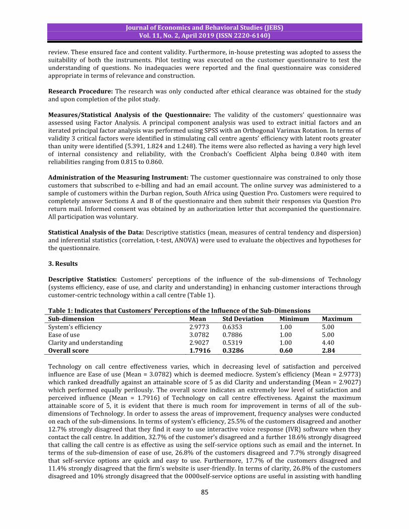
Journal of Economics and Behavioral Studies (JEBS) Vol. 11, No. 2, April 2019 (ISSN 2220-6140)
85
review. These ensured face and content validity. Furthermore, in-house pretesting was adopted to assess the suitability of both the instruments. Pilot testing was executed on the customer questionnaire to test the understanding of questions. No inadequacies were reported and the final questionnaire was considered appropriate in terms of relevance and construction. Research Procedure: The research was only conducted after ethical clearance was obtained for the study and upon completion of the pilot study. Measures/Statistical Analysis of the Questionnaire: The validity of the customers’ questionnaire was assessed using Factor Analysis. A principal component analysis was used to extract initial factors and an iterated principal factor analysis was performed using SPSS with an Orthogonal Varimax Rotation. In terms of validity 3 critical factors were identified in stimulating call centre agents’ efficiency with latent roots greater than unity were identified (5.391, 1.824 and 1.248). The items were also reflected as having a very high level of internal consistency and reliability, with the Cronbach’s Coefficient Alpha being 0.840 with item reliabilities ranging from 0.815 to 0.860. Administration of the Measuring Instrument: The customer questionnaire was constrained to only those customers that subscribed to e-billing and had an email account. The online survey was administered to a sample of customers within the Durban region, South Africa using Question Pro. Customers were required to completely answer Sections A and B of the questionnaire and then submit their responses via Question Pro return mail. Informed consent was obtained by an authorization letter that accompanied the questionnaire. All participation was voluntary. Statistical Analysis of the Data: Descriptive statistics (mean, measures of central tendency and dispersion) and inferential statistics (correlation, t-test, ANOVA) were used to evaluate the objectives and hypotheses for the questionnaire. 3. Results Descriptive Statistics: Customers’ perceptions of the influence of the sub-dimensions of Technology (systems efficiency, ease of use, and clarity and understanding) in enhancing customer interactions through customer-centric technology within a call centre (Table 1). Table 1: Indicates that Customers’ Perceptions of the Influence of the Sub-Dimensions Sub-dimension Mean Std Deviation Minimum Maximum System’s efficiency 2.9773 0.6353 1.00 5.00 Ease of use 3.0782 0.7886 1.00 5.00 Clarity and understanding 2.9027 0.5319 1.00 4.40 Overall score 1.7916 0.3286 0.60 2.84 Technology on call centre effectiveness varies, which in decreasing level of satisfaction and perceived influence are Ease of use (Mean = 3.0782) which is deemed mediocre. System’s efficiency (Mean = 2.9773) which ranked dreadfully against an attainable score of 5 as did Clarity and understanding (Mean = 2.9027) which performed equally perilously. The overall score indicates an extremely low level of satisfaction and perceived influence (Mean = 1.7916) of Technology on call centre effectiveness. Against the maximum attainable score of 5, it is evident that there is much room for improvement in terms of all of the sub-dimensions of Technology. In order to assess the areas of improvement, frequency analyses were conducted on each of the sub-dimensions. In terms of system’s efficiency, 25.5% of the customers disagreed and another 12.7% strongly disagreed that they find it easy to use interactive voice response (IVR) software when they contact the call centre. In addition, 32.7% of the customer’s disagreed and a further 18.6% strongly disagreed that calling the call centre is as effective as using the self-service options such as email and the internet. In terms of the sub-dimension of ease of use, 26.8% of the customers disagreed and 7.7% strongly disagreed that self-service options are quick and easy to use. Furthermore, 17.7% of the customers disagreed and 11.4% strongly disagreed that the firm’s website is user-friendly. In terms of clarity, 26.8% of the customers disagreed and 10% strongly disagreed that the 0000self-service options are useful in assisting with handling

Journal of Economics and Behavioral Studies (JEBS) Vol. 11, No. 2, April 2019 (ISSN 2220-6140)
86
their queries. Furthermore, 38.6% of the customers disagreed and 19.5% strongly disagreed that they frequently visit blogs to share information about their service encounter with the firm. Inferential Statistics Hypothesis 1: There exists significant intercorrelations amongst the sub-dimensions of Technology (systems efficiency, ease of use, and clarity and understanding) respectively. Table 2: Pearson Correlation (r): Inter Correlations of the Influence of Technology (N = 220) Sub-dimension r/p Systems efficiency Ease of use Clarity and understanding
Systems efficiency r p
1
Ease of use r p
0.463 0.000**
1
Clarity and understanding
r p
0.519 0.000**
0.687 0.000**
1
Note: **p <0.01 Table 2 indicates that the precarious constituents anticipated by customers in their interactions with the call centre significantly intercorrelate with each other at the 1% level of significance. Therefore, hypothesis 1 may be accepted. Table 2 indicates strong relationships between ease of use of technology (r = 0.463) and clarity and understanding of systems adopted within the call centre (r = 0.687), respectively. The significant intercorrelations between the dicey constituents of technology indicates that if these dynamics are enriched and developed, it has the potential to have a positive spin-off effect on the communication between the customer and the call centre thereby boosting superior service delivery, greater customer satisfaction and enriched overall efficiency. Influence of Biographical Data: The influence of the biographical variables (age, race, gender and education) on customers’ perceptions of the sub-dimensions of Technology was assessed using ANOVA and t-tests (Table 3). Hypothesis 2: Customers varying in biographical variables (age, race, gender and education) significantly differ in their perceptions of the sub-dimensions of Technology (systems efficiency, ease of use, and clarity and understanding) respectively. Table 3: Biographical Variables and the Customers’ Perceptions of the Sub-Dimensions of Technology ANOVA Sub-dimensions of Technology Biographical Variable Age Race Educational
Qualification F p F p F p Systems Efficiency 0.384 0.820 0.078 0.972 0.105 0.957 Ease of Use 1.162 0.329 2.359 0.073 0.193 0.901 Clarity and understanding 0.395 0.812 0.337 0.798 0.399 0.754 t-TEST Sub-dimensions of Technology Biographical Variable Gender T p Systems Efficiency -1.765 0.079 Ease of Use -1.508 0.133 Clarity and understanding -0.441 0.660
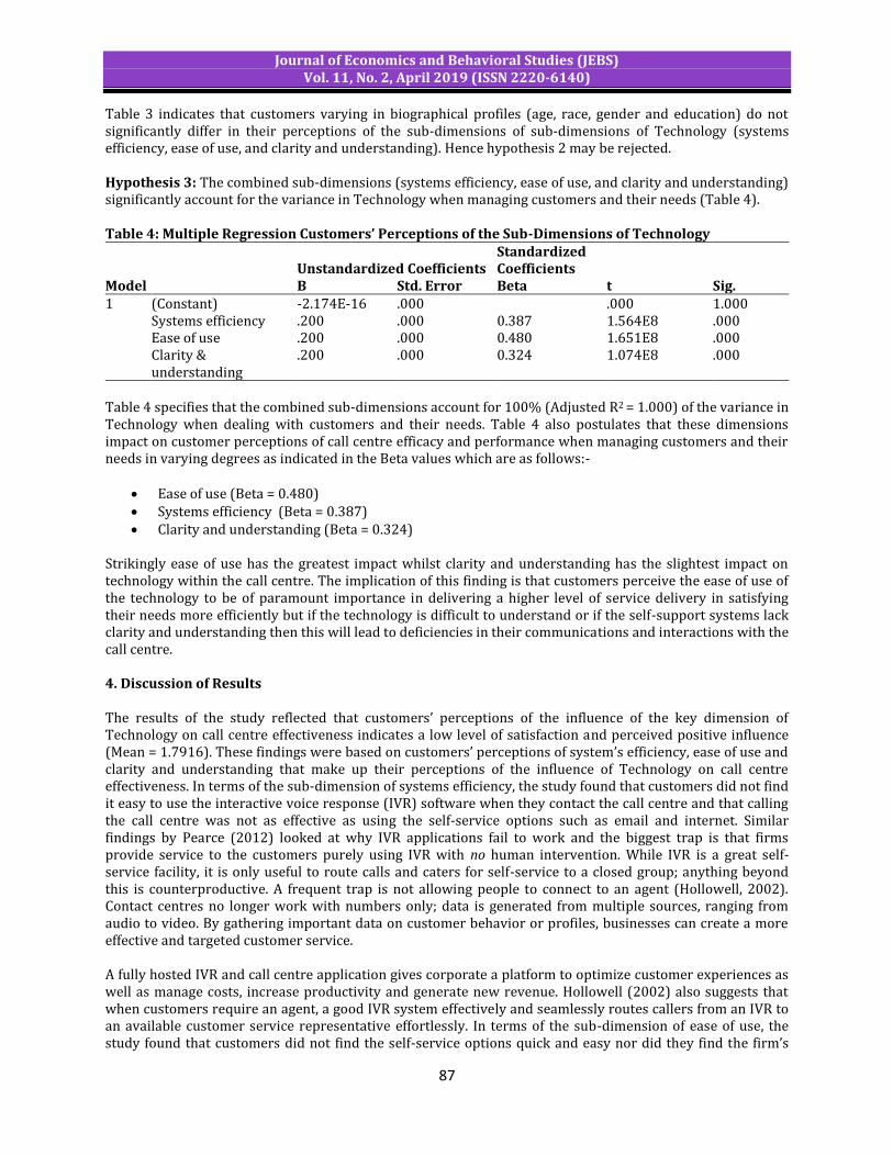
Journal of Economics and Behavioral Studies (JEBS) Vol. 11, No. 2, April 2019 (ISSN 2220-6140)
87
Table 3 indicates that customers varying in biographical profiles (age, race, gender and education) do not significantly differ in their perceptions of the sub-dimensions of sub-dimensions of Technology (systems efficiency, ease of use, and clarity and understanding). Hence hypothesis 2 may be rejected. Hypothesis 3: The combined sub-dimensions (systems efficiency, ease of use, and clarity and understanding) significantly account for the variance in Technology when managing customers and their needs (Table 4). Table 4: Multiple Regression Customers’ Perceptions of the Sub-Dimensions of Technology
Model Unstandardized Coefficients
Standardized Coefficients
t Sig. B Std. Error Beta 1 (Constant) -2.174E-16 .000 .000 1.000
Systems efficiency .200 .000 0.387 1.564E8 .000 Ease of use .200 .000 0.480 1.651E8 .000 Clarity & understanding
.200 .000 0.324 1.074E8 .000
Table 4 specifies that the combined sub-dimensions account for 100% (Adjusted R2 = 1.000) of the variance in Technology when dealing with customers and their needs. Table 4 also postulates that these dimensions impact on customer perceptions of call centre efficacy and performance when managing customers and their needs in varying degrees as indicated in the Beta values which are as follows:-
Ease of use (Beta = 0.480) Systems efficiency (Beta = 0.387) Clarity and understanding (Beta = 0.324)
Strikingly ease of use has the greatest impact whilst clarity and understanding has the slightest impact on technology within the call centre. The implication of this finding is that customers perceive the ease of use of the technology to be of paramount importance in delivering a higher level of service delivery in satisfying their needs more efficiently but if the technology is difficult to understand or if the self-support systems lack clarity and understanding then this will lead to deficiencies in their communications and interactions with the call centre. 4. Discussion of Results The results of the study reflected that customers’ perceptions of the influence of the key dimension of Technology on call centre effectiveness indicates a low level of satisfaction and perceived positive influence (Mean = 1.7916). These findings were based on customers’ perceptions of system’s efficiency, ease of use and clarity and understanding that make up their perceptions of the influence of Technology on call centre effectiveness. In terms of the sub-dimension of systems efficiency, the study found that customers did not find it easy to use the interactive voice response (IVR) software when they contact the call centre and that calling the call centre was not as effective as using the self-service options such as email and internet. Similar findings by Pearce (2012) looked at why IVR applications fail to work and the biggest trap is that firms provide service to the customers purely using IVR with no human intervention. While IVR is a great self-service facility, it is only useful to route calls and caters for self-service to a closed group; anything beyond this is counterproductive. A frequent trap is not allowing people to connect to an agent (Hollowell, 2002). Contact centres no longer work with numbers only; data is generated from multiple sources, ranging from audio to video. By gathering important data on customer behavior or profiles, businesses can create a more effective and targeted customer service. A fully hosted IVR and call centre application gives corporate a platform to optimize customer experiences as well as manage costs, increase productivity and generate new revenue. Hollowell (2002) also suggests that when customers require an agent, a good IVR system effectively and seamlessly routes callers from an IVR to an available customer service representative effortlessly. In terms of the sub-dimension of ease of use, the study found that customers did not find the self-service options quick and easy nor did they find the firm’s

Journal of Economics and Behavioral Studies (JEBS) Vol. 11, No. 2, April 2019 (ISSN 2220-6140)
88
website to be user-friendly. Similar findings by Dabholkar, Bobbitt & Lee (2003) and Weijters, Rangarajan, Falk & Schillewaert (2007) suggest that self-service technology has had limited success in retail settings. The primary reason for this was due to the lack of understanding of consumers assessment associated with the usage of self-service technology. Conversely, the Economist (2009) & Wang (2012) suggest that self-service technology is gaining prominence. This service encourages consumers to produce the service independent of the service employees’ involvement and results in improvements in the retailer’s productivity and service quality (Lee, Fairhurst & Lee, 2009). Finally, in terms of the sub-dimension of clarity and understanding, the study found that customers did not find the self-service options to be useful in assisting with the handling of queries and many did not visit blogs to share information about their service encounter with the firm. Similar studies by Makarem, Mudambi & Padoshen (2009) found that it’s not possible to have a single services option to satisfy everyone. In their study some customers preferred technology whilst others preferred human contact. Managers should profile the attitudes of consumers towards technology and interpersonal service encounters as it’s not possible to offer only one method of service contact and delivery to consumers. Conversely, Hsieh (2005) proposes that self-service technology (SST) can lead to greater customer service, empowered customers and employees and improved efficiency. Communication is the key to adoption of new technology; listen to what the customer wants and have a protective and reassuring plan for privacy and security to ensure adoption of self-service more readily. In summary, the key finding of the study was predominantly that Customers did not find it easy to use Interactive Voice Response (IVR) and found that calling the call centre was not as effective as using the self-service options. Additionally, the self-service options were not quick and easy to use neither was the website user-friendly. Finally, self-service options were not useful in handling customer queries and customers did not visit blogs to share information about service experiences. 5. Recommendations and Conclusion Although technology has led to a loss of empathy on the front line and has resulted in a weakening of customer care, newer technologies, if well deployed, can help overcome the problem. Gorry & Westbrook (2011) suggest that the three ways that firms can improve their customer care are by improving its self-service customer care channels, helping front-line employees respond empathetically and exploiting social networks to better care for customers. Technology has become a key enabler in delivering high levels of service; however, over-reliance on technology can impact negatively on service quality (Jack & McCary, 2006). The question that one needs to ask is whether technology-based services can provide the same high level of service that customers expect as they do from interpersonal service providers. As we have seen from the literature, if implemented correctly technology has the potential to save the organization a lot of money in the long run; however, the literature also suggests that over-reliance on self-service technology to the point of phasing out human contact could have disastrous consequences for the organization so it becomes imperative to be able to strike a balance and open up the lines of communication (Jack & McCary, 2006). In addition, waiting lines are a major deterrent in a call centre irrespective of whether the call centre offers self-service options or whether the customer has to hold for an agent. Research by Peevers et al. (2009) suggest that listening to music can lead to the perception of shorter waiting times while the customer is waiting in the queue but in the long run, long waits should be avoided. In terms of customers’ perceptions of the influence of the sub-dimensions of Technology on call centre effectiveness, the following recommendations are suggested in terms of System’s efficiency: Customers did not find it easy to use the Interactive Voice Response (IVR) and found that calling the call centre was not as effective as using the self-service options such as e-mail and internet. Upgrade the IVR system to improve response rates and upgrade the software technology in the call centre to improve turnaround times. Cloud technology solutions are at the forefront of shaping the field of contact centre services. Contact centres that migrate to the cloud are investing in a better experience for their customers (Business Tech, 2017). In terms of ease of use Self-service option were not quick and easy to use nor was the website user-friendly. It is suggested that the website be upgraded to include more self-help links. More Frequently Asked Questions should be uploaded; quicker software technology should be adopted to make the website easily accessible and downloadable. Website information should also contain key information and access to links that make it easy for consumers
Journal of Economics and Behavioral Studies (JEBS) Vol. 11, No. 2, April 2019 (ISSN 2220-6140)
89
to access quickly and easily taking into consideration linguistic preferences of consumers, site navigation should also be easy, site design should be attractive and appealing. Tagged as the most critical business tool for contact centres, the omni-channel approach includes, amongst others, emails, phone calls, texts, chatbots and customer forums. This approach enables customers to interact with multiple channels and the challenge for these channels is to ensure that this is a seamless experience for the customer. Delivering this approach through a customer service centre has many profits, but primarily it ensures that quality and consistency of service across all channels is accomplished and sustained. And finally clarity and understanding: Self-service options were not useful in handling customer queries and customers did not visit blogs to share information about service experiences. It is evident that customers are not too tech savvy and still prefer doing business using conservative methods. It is suggested that although it is important for the organization to be familiar with modern technology in terms of doing business, not to ignore conventional methods of sharing information with customers either. The majority of customers still use these conservative methods to do business. Strike a balance between old and new forms of communication such as through blogs and conventional newsletters such that you still reach both target audiences timeously. Recommendations for Future Research: This research was undertaken in one public service call centre and hence, the results of the study have internal validity to this organization. In order to enrich generalizability, it would be beneficial to undertake a comparative study within other call centre environments in a variety of service environments in both the public and private sectors. This study also includes a call centre environment where only inbound calls are made and hence, it would be beneficial to evaluate related dimensions in an outbound call setting as interacting with someone who has chosen to interact with you is completely different from interacting with someone who was not expecting your interaction at all. References Beirre, M., Riach, K. & Wilson, F. (2004). Controlling Business? Agency and Constraint in call centre Working.
New Technology, Work and Employment, 19(2), 96–109. Bendoly, E., Rosenzweig, E. & Stratman, J. (2009). The efficient use of enterprise information for strategic
advantage: a data envelopment analysis, Journal of Operations Management, 27(4), 310-23. Borck, J. R. (2004). Successful E-Services. Internet. Burgess, J. & Connell, J. (2004). Emerging Developments in call centre research. Labour and Industry, 14(3), 1-
13. Burke, J. (2001). Relationship aspect Marketing Building customer loyalty in the Internet Age. USA: Silver
Lake Publishing. Business Tech. (2017). How to improve your customer service with communications technology. Cheng, L., Gibson, M., Carrillo, E. & Fitch, G. (2011). A technology-centric framework for investigating business
operations, Industrial Management & Data Systems, 111(4), 509-30. Cheong, K., Kim, J. & So, S. (2008). A study of strategic call centre management: relationship between key
performance indicators and customer satisfaction, European Journal of Social Sciences, 6(2), 268-276. Clegg, B. (2010). Agency-to-Carrier collaboration key to Drive Claims-Handling Improvements. Dabholkar, P. A., Bobbit, L. M., Lee, E. J. (2003). Understanding consumer motivation and behavior related to
self-scanning in retailing. International Journal of Service Industry Management, 14(1), 59-95. Dean, A. (2007). The impact of the customer orientation of call centre employees on customers: affective
commitment and loyalty, Journal of Service Research, 10(2), 161-173. Dixon, P. (2002). Future wise: Six faces of Global changes. Profile Books. London. Economist. (2009). The recession spurs self-service: help yourself. Ellis, V. & Taylor, P. (2006). You don’t know what you’ve got till it’s gone: re-contextualising the origins,
development and impact of the call centre, New Technology, Work and Employment, 21(2), 107–122. Fichter, D. & Wisniewski, J. (2010). Practical Website Improvement Face-off. Fitzsimmons, J. A. & Fitzsimmons, M. J. (2006). Service Management: Operations, Strategy and Information
Technology. Fifth Edition. New York: McGraw-Hill/Irwin.

Journal of Economics and Behavioral Studies (JEBS) Vol. 11, No. 2, April 2019 (ISSN 2220-6140)
90
Gelderman, C., Ghijsen, P. & van Diemen, R. (2011). Choosing self-service technologies or interpersonal services – the impact of situational factors and technology-related attitudes, Journal of Retailing and Consumer Services, 18(5), 414-21.
Geum, Y., Lee, S., Kang, D. & Park, Y. (2011). Technology road mapping for technology-based product-service integration: a case study, Journal of Engineering and Technology Management, 28(3), 128-46.
Gorry, G. A. & Westbrook, R. A. (2011). Once more, with feeling: Empathy and technology in customer care. Business Horizons, 54, 125-134.
Girman, G., Keusch, P. & Kmec, P. (2009). Faults, failures and availability in Self-Service Technology. Hollowell, R. (2002). Service on the Internet: the effect of physical service on scalability. Harvard Business
Review. How Technology is changing the Call Centre. (2017). Hsieh, C. T. (2005). Implementing Self-service technology to gain competitive advantages. Communications of
IlMA, 5(1), 77-83. Jack, E. P., Bedics, T. A. & McCary, C. E. (2006). Operational Challenges in a call centre industry: a case study
and resource-based framework. Managing Service Quality, 16(5), 477-500. Keaggy, B. & Hurst, M. (2002). Face-off are Weblogs legitimate Business Tools? Lavin, D. & Maynard, D. (2001). Standardization vs rapport: respondent laughter and interviewer reaction
during telephone surveys, American Sociological Review, 66, 453-79. Lee, H. J., Fairhurst, A. E. & Lee, M. Y. (2009). The importance of self-service kiosks in developing consumers
retail patronage intentions. Managing Service Quality, 19(6), 687-701. Lin, J. & Hsieh, P. (2011). Assessing the self-service technology encounters: development and validation of
SSTQUAL scale, Journal of Retailing, 87(2), 194-206. Lu, J., Chou, H. & Ling, P. (2009). Investigating passengers’ intentions to use technology-based self-check-in
services, Transportation Research Part E: Logistics and Transportation Review, 45(2), 345-56. Lu, J. & Zhang, G. (2003). Cost-benefit-factor analysis in e-services. Lucas, R. W. (2005). Customer Service: Building successful skills for the 21st Century. Third Edition. New
York: McGraw-Hill/Irwin. Makarem, S., Mudambi, S. & Podoshen, J. (2009). Satisfaction in technology-enabled service encounters”,
Journal of Services Marketing, 23(3), 134-44. Malgeri, A. (2007). Customer service and self-service technology. Mattila, A., Cho, W. & Ro, H. (2011). The role of self-service technologies in restoring justice”, Journal of
Business Research, 64(4), 348-55. Metters, R., Metters, K. K., Pullman, M. & Walton, S. (2006). Successful Service Operations Management.
Second Edition. USA: Thomson South-Western. Ojiako, U. (2012). Using IS/IT to enhance service delivery”, Industrial Management & Data Systems, 112(4),
584-599. Pearce, J. (2012). The seven deadly sins of IVR. Peevers, G., McInnes, F., Morton, H., Matthews, A. & Jack, M. A. (2009). The mediating effects of brand music
and waiting time updates on customers’ satisfaction with a telephone service when put on-hold. International Journal of Bank Marketing, 27(3), 202-217.
Perez, J. C. (2004). Dell hopes support hubs will improve service delivery. Piercy, N. & Rich, N. (2009). High Quality and low cost: the Lean service centre, European Journal of
Marketing, 43(11/12), 1477-1497. Reinders, M., Dabholkar, P. & Frambach, R. (2008). Consequences of forcing consumers to use technology-
based self-service, Journal of Service Research, 11(2), 107-23. Reichheld, F. F., Sasser, W. E. & Jr. (1990). Zero Defections: Quality comes to Service. Robertson, N. & Shaw, R. (2009). Predicting the likelihood of voiced complaints in the self-service technology
context, Journal of Service Research, 12(1), 100-16. Rowley, J. (2006). An analysis of the e-service literature: towards a research agenda. Ruyter, K., Wetzels, M. & Kleijnen, M. (2000). Customer’s adoption of e-service: an experimental study. Schiffman, L. G. & Kanuk, L. L. (2004). Consumer Behavior. Eighth Edition. New Jersey: Pearson Prentice Hall. Sims, D. (2011). The benefits of IVR in Retail. Timm, P. R. (2008). Customer Service: Career Success through Customer Loyalty. Fourth Edition. USA:
Pearson Prentice Hall.

Journal of Economics and Behavioral Studies (JEBS) Vol. 11, No. 2, April 2019 (ISSN 2220-6140)
91
Venkatesh, V. & Agarwal, R. (2006). Turning visitors into customers: a usability-centric perspective on purchase behaviour in electronic channels, Management Science, 52(3), 367-82.
Wang, M. C. H. (2012). Determinants and consequences of consumers satisfaction with self-service technology in a retail setting. Managing Service Quality, 22(2), 128-144.
Weijters, B., Rangarajan, D., Falk, T. & Schillewaert, N. (2007). Determinants and outcomes of customers use of self-service technology in retail setting. Journal of Service Research, 10(1), 3-21.
Whiting, A. & Donthu, N. (2006). Managing voice-to-voice encounters: reducing the agony of being put on hold, Journal of Service Research, 8(3), 234–244.
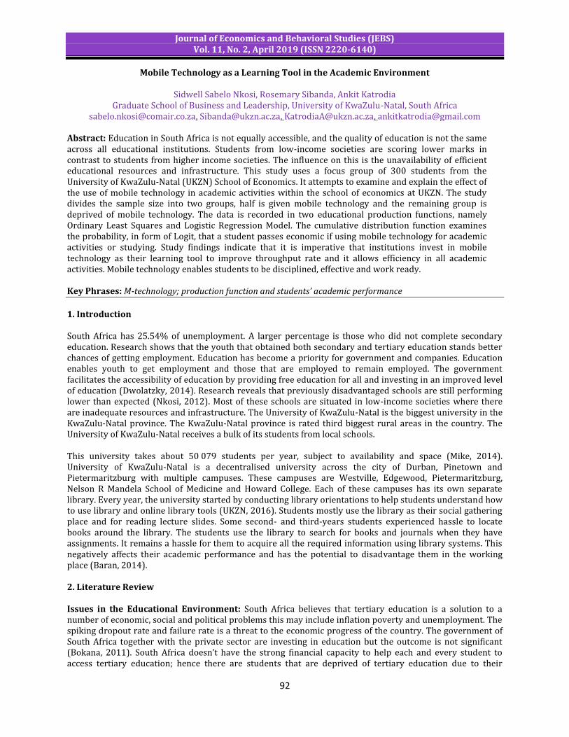
Journal of Economics and Behavioral Studies (JEBS) Vol. 11, No. 2, April 2019 (ISSN 2220-6140)
92
Mobile Technology as a Learning Tool in the Academic Environment
Sidwell Sabelo Nkosi, Rosemary Sibanda, Ankit Katrodia Graduate School of Business and Leadership, University of KwaZulu-Natal, South Africa
[email protected], [email protected], [email protected], [email protected] Abstract: Education in South Africa is not equally accessible, and the quality of education is not the same across all educational institutions. Students from low-income societies are scoring lower marks in contrast to students from higher income societies. The influence on this is the unavailability of efficient educational resources and infrastructure. This study uses a focus group of 300 students from the University of KwaZulu-Natal (UKZN) School of Economics. It attempts to examine and explain the effect of the use of mobile technology in academic activities within the school of economics at UKZN. The study divides the sample size into two groups, half is given mobile technology and the remaining group is deprived of mobile technology. The data is recorded in two educational production functions, namely Ordinary Least Squares and Logistic Regression Model. The cumulative distribution function examines the probability, in form of Logit, that a student passes economic if using mobile technology for academic activities or studying. Study findings indicate that it is imperative that institutions invest in mobile technology as their learning tool to improve throughput rate and it allows efficiency in all academic activities. Mobile technology enables students to be disciplined, effective and work ready. Key Phrases: M-technology; production function and students’ academic performance
1. Introduction South Africa has 25.54% of unemployment. A larger percentage is those who did not complete secondary education. Research shows that the youth that obtained both secondary and tertiary education stands better chances of getting employment. Education has become a priority for government and companies. Education enables youth to get employment and those that are employed to remain employed. The government facilitates the accessibility of education by providing free education for all and investing in an improved level of education (Dwolatzky, 2014). Research reveals that previously disadvantaged schools are still performing lower than expected (Nkosi, 2012). Most of these schools are situated in low-income societies where there are inadequate resources and infrastructure. The University of KwaZulu-Natal is the biggest university in the KwaZulu-Natal province. The KwaZulu-Natal province is rated third biggest rural areas in the country. The University of KwaZulu-Natal receives a bulk of its students from local schools. This university takes about 50 079 students per year, subject to availability and space (Mike, 2014). University of KwaZulu-Natal is a decentralised university across the city of Durban, Pinetown and Pietermaritzburg with multiple campuses. These campuses are Westville, Edgewood, Pietermaritzburg, Nelson R Mandela School of Medicine and Howard College. Each of these campuses has its own separate library. Every year, the university started by conducting library orientations to help students understand how to use library and online library tools (UKZN, 2016). Students mostly use the library as their social gathering place and for reading lecture slides. Some second- and third-years students experienced hassle to locate books around the library. The students use the library to search for books and journals when they have assignments. It remains a hassle for them to acquire all the required information using library systems. This negatively affects their academic performance and has the potential to disadvantage them in the working place (Baran, 2014). 2. Literature Review Issues in the Educational Environment: South Africa believes that tertiary education is a solution to a number of economic, social and political problems this may include inflation poverty and unemployment. The spiking dropout rate and failure rate is a threat to the economic progress of the country. The government of South Africa together with the private sector are investing in education but the outcome is not significant (Bokana, 2011). South Africa doesn’t have the strong financial capacity to help each and every student to access tertiary education; hence there are students that are deprived of tertiary education due to their

Journal of Economics and Behavioral Studies (JEBS) Vol. 11, No. 2, April 2019 (ISSN 2220-6140)
93
inability to pay the fees. The University of KwaZulu-Natal has been engaged in serious research around students’ academic progress. There might be opportunities for hidden talent from those students that are deprived of tertiary education. Numerous studies that have been conducted around students’ performance depict a common outcome. The outcome is measured through the number of students who graduated within the minimum prescribed period for a degree. A study conducted by Mike 2014, an exhibit that from 2004-2012, 42% of students graduated within the space of the minimum degree period. Students that were academically excluded make up to 19.45%, the amount of 6.98% of students dropped out with a good academic record, the rest is still studying, 31.39%. This study will base some of its foundation on Papert’s and Piaget’s constructivism. Piaget looks at what are children’ interests, what are they capable of achieving at their different stages of growth. Piaget’s theory looks deeper on child’s life and explains their ways of thinking and doing the thing as they grow and it analyses different circumstances in which a child changes their worldviews or hold into their worldviews (Ackermann, 2016). On the other hand, Papert’s constructionism explains the art of learning. In this study, Papert’s theory will be adopted. Papert’s research focused on how learners learning to learn by looking at how they engage themselves into conversations with other people, their own or artefacts and how conversations improve self-direct learning and the construction of new knowledge. In order to construct new knowledge, the use of media, tools and context in human development is essential (Ackermann, 2016). Technology has primarily reshaped our lifestyle, way in which we work and communicate with others. It further influences the education system, thus it became the most used and the essential tool to construct new knowledge (Lan Li, 2015). Individuals are driven by a sense of self-efficacy to perform their daily life activities. Self-efficacy is defined by Efe (2015) he stated that it is the formation of behaviour self-perception, belief and judgement of an individual’s capacity in planning the necessary activity to achieve something under different situations. For this context, self-efficacy refers to the use of technology. Perceived computer self-efficacy as an individual’s accepted perception of his ability to use the computer to do tasks that are required to be done by a computer (Efe, 2015). The advancement of technology has encouraged the use of technology by all range of ages and in everyday life activities. This may be due to its portability and affordability (Baran, 2014). Large funds of investment have been allocated to technology to integrate mobile technology with the learning system and many researchers have focused their interest in the evolving landscape. But there are some hinders like lack of theoretical and pedagogical outlining sustainable interlink with formal education context and unavailability of teachers support and training (Baran, 2014). The accessibility of mobile devices like personal computers, tablets and smartphones have made mobile devices common to the youth. The development of Applications (Apps) and mobile service made technological devices popular (Kateryna, 2015). All these mobile devices are user-friendly and most people use them to access news, financial information, entertainment, learning etc. In the past, technological limits made technology not to be used for educational purposes. Challenges like limited internet access, expensiveness, insufficient memory space, are now resolved to enable maximum use of technology for mobile learning. Therefore, m-learning became the platform to provide many educational activities. It is used for different purposes and for different needs, it may be used to deliver content or focus on training for jobs. It can also be in the form of learning application, performance support, to access learning materials by secondary institutions’ students and higher educations’ students. Health professionals are using podcasts as a form of mobile learning, which is lately an important technological tool (Kalludi, 2015). Academic Performance in the School of Economics: The throughput rate is an issue that many schools within the University of KwaZulu-Natal facing (Essack, 2014). It is not feasible that this study is performed for each and every school because the University of KwaZulu-Natal is big and consists of a number of schools. The main attention of this study will be narrowed to the School of Economics at the University of KwaZulu-Natal Westville Campus. The high failure rate and dropout rate in the School of Economics have come to the attention of the gatekeepers who are responsible for a variety of degree programmes and qualifications in the school. There are many factors that attribute to this issue it could be low-quality secondary education, the bigger transition between universities and secondary education. Some researchers proclaimed that economics is a difficult module (Bokana, 2011). In this study Economics 102 and Economics 201 will be
Journal of Economics and Behavioral Studies (JEBS) Vol. 11, No. 2, April 2019 (ISSN 2220-6140)
94
analysed. From 2013, 2014 and 2015, the pass rate was 69.20%, 67.48% and 80.36% correspondingly. The performance for Economics 102 module exhibits an upward trend with a spike in 2015. The performance for Economics 201 module from 2013, 2014 and 2015 is 65.68%, 65.26% and 78.53% respectively. Economics 102 modules and Economics 201 module both have upward trends but Economics 201 module is relatively below Economics 102 module. This may result in the class overcrowding by 1.83% for economics 201 modules in 2016. When the class is overcrowded, it’s not easy for students to pass because of limited space in the class and some students are discouraged from attending. This may shrink the pass rate compared to last years. The higher the failure rate for Economics 102 module and Economics 201 modules is the higher the chances of the university taking fewer new entrant students who want to study economics. This is an issue of concern, not only for UKZN but for all tertiary institutions. Improving the quality and equity of students’ academic performance remains, therefore, remains the top priority for the South African Higher Education (Vithal, 2015). Mobile Technology as a Solution: The modern people’s social and economic lifestyle is dependent to the invention of smart and portable technology, this is personal computers, smartphones, tablets and internet (EL-Hhussein, 2010). The common use for these smart technological devices is getting access to the internet to keep up with the news, emails, financial updates, social media and communication (Danylova, O., Manako, A., Synytsya, K. & Voychenko, O. 2004). Most people are attracted to using these devices because they are portable and for their wireless functionality. M-Technology is used as a tool that provides education in different organisations. It is also used for content delivery for specific training in a job, performance support or extra access to learning material for secondary and higher education institutions for students (EL-Hussein, 2010). The continuous advancement of technology is positively influencing life from all spheres. Most researchers are interested in the impact of changing technology in education (Kim, 2013). The society that is technological sound gives rise to new opportunities for learning. Not many years ago the learning environment evolved into e-learning and m-learning environment (Kim, 2013), students are utilising all the different kinds of technology to learn. Common learning technological devices are Personal Digital Assistant (PDA), Ultra Mobile PC (UMPC) PC etc. Each device is developed for its different purpose many applications and software are created to make these devices more usable. The differences are highlighted in the purpose for which these devices are created for they come in different sizes with regards to mobility and portability. The beauty of mobile technology is that it can extend classroom lessons to distance network places. The newly developed technology like cameras, embedded sensors, location awareness, motion detection, social network, web searching and augmented reality, shows the need to upgrade learning and enable it to take place at different remote places, conceptual and social spaces, outdoor and indoor (Baran, 2014). Mobile technology enables lectures and students to gain unconstrained access to information, expediency, convenience, immediacy. The features provided by this technology add value to the quality of lecturing and enhance the students; learning. Such features offer a chance for individualisation, collaborative, situated, and informal learning exclusive of classroom context limits (Baran, 2014). Quinn and Stein (2013) have directed the focus to the vital roled played by e-learning to upgrading future education for online schools and traditional schools. Maysami (2015) says there is direct instruction from traditional classes which is directed to the whole class, the speed of learning is monitored by a lecturer and they follow the textbook curriculum. The availability of e-tools that are applicable for both face-to-face and online formats enables students to take a lead in the learning programmes and play a more pro-active part. The fast pace advancement of technology has transformed education, making it digital and accessible by almost everyone and everywhere. E-learning allows and attracts everyone, all ages, all nations, all races to obtain learning through its multiple space capability and elastic times (Maysami, 2015). Online courses are enough for students provided that there are extra assistant tools like lecture slides, bulletin boards, online assessments. Other students are very reluctant to migrate to e-learning. They still prefer traditional learning and only search for extra help online, but not relying online (Quinn & Stein 2013). To make online educational tools more usable, online courses are structured well and interactive to create a user-friendly environment
Journal of Economics and Behavioral Studies (JEBS) Vol. 11, No. 2, April 2019 (ISSN 2220-6140)
95
(Tucker, 2012). Open Australia University is regarded as the pioneer of e-learning. It experienced a doubled amount of student enrolment after fully introducing e-learning (Johnson, 2015). Above 70% of the universities at the United States of America are providing e-learning programs (Johnson, 2015). Full e-learning students are self-controlled and much disciplined because they have to set their learning goals, identify a proper learning strategy and put it into place (Johnson, 2015). The University of KwaZulu-Natal recently adopted mobile technology for its learning purposes. The integration of mobile technology and teaching and learning gives hope that the pass rate at the University of KwaZulu-Natal will improve (UKZN, 2016). The implementation of these technological tools goes together with certain challenges, which if disregarded defeat the purpose implementation of m-technology (Ramorola, 2013). The challenges may include the attitude and usage of these tools by academic staff and students, affordability of these technologies, unavailability of technology policy, lack of teachers/lecturers qualified in technology integration and maintenance of these technologies (Baran, 2014). It is against this background that this study set out to find if the introduction of m-learning at UKZN can improve economics students’ pass rate. 3. Methodology This study attempts to test if the uses of mobile technology can improve economics students’ pass rate. The technique adopted in this study is a quantitative research technique. This type of method is the systematic empirical investigation of observable phenomena via statistical, mathematical or computation techniques. Research Design: The proposed research approach for this study is quantitative research using a cross-sectional study. A quantitative research is an investigation into social or human problems based on testing a theory composed of variables, measured with numbers and analysed with statistical procedures to determine whether the predictive generalisation of the theory is true (Bokana, 2011). The cross-sectional study obtains data once at a specific time and in a specific place (McBride, 2016). It is further used to investigate associations between factors and outcomes within a defined population. Aim of the Study: This study aims to find out if the use of mobile technology would improve the economics students’ academic performance at the University of KwaZulu-Natal. To achieve that, the researcher needs to find out if the students that are given mobile technology could perform well than those students that are not given mobile technology. In the process, other important factors that come in as the important determinates for academic performance will be incorporated. Those factors include demography and attitude towards mobile technology. The researcher also wants to establish the degree at which technology impacts the students’ academic performance. Data Collection: This study uses a quantitative technique to collect data. Primary data will be used in this study; however, existing statistical data will be used as a frame of reference. To get the data required for this study, a questionnaire was designed. A questionnaire had 7 sections; first section contained information regarding the researcher, supervisor, definitions, message to the participants and a consent form. Second section asked information concerning participants’ demography third section focuses on participants’ academic characteristics. Section four to the last section asked questions based on the objectives of this study. The four-point Likert scale is used. A number of 2119 UKZN students are currently registered for economics module 101 and module 102 (UKZN, 2016). All these students are reachable through emails and Moodle Learning Site. Questionnaires were designed using google forms. There was no issue of hard copy questionnaires. Questionnaires, informed consent form and a message explaining more about the survey will be sent to students via institution emails and a message will be posted on Moodle Learning Site. This was done to encourage the students to fill in the survey form. The email will contain a URL that students must click and it will direct them straight to the form. After they have filled in the form, they must click a text box saying submit. The data will automatically be updated to the online spreadsheet which is linked with Google form. To improve the respondents’ rate, tutors and lectures will be advised to encourage students to fill in the survey forms. Data Quality Control: This study uses a quantitative research method data was monitored to ensure validity and reliability. Validity is very important to make sure that data addresses what it supposed to address. To ensure correct measure of the objectives, all questionnaires were closed questions. Reliability test was

Journal of Economics and Behavioral Studies (JEBS) Vol. 11, No. 2, April 2019 (ISSN 2220-6140)
96
conducted to ensure that the same results are yield at any time under similar conditions (Creswell and Clark, 2007:350). Sampling Strategy: The entire data required for this research is collected at the University of KwaZulu-Natal (Westville- Main Campus). The research focuses on economics students, so they are the only required participants for this study. The school of economics has 2119 students that are currently registered for both economics 101 module and economics 201 (UKZN, 2016). The sampling strategy that is adopted in this study is the probability sampling. In the form there is field that requires first three digits of the students’ number and the other field requires an academic year of the participants. This information is used to separate data into 2 groups, first year and second years based on their academic year. The first three digits of their students’ number will be used to identify if the student is a repeater or not. The data will also account for transferred students. Those students would have students’ numbers starting with 216xxx but a student would be in their second year of study (academic year). Since the researcher wanted to test the influence of mobile technology determinant in the students’ academic performance, students whose students’ numbers start with 216xxx and in their first year of study are assumed to have mobile technology. The University of KwaZulu-Natal clearly outlined that all the first-year students are required to have personal computers as the primary requirement for the university in order to be admitted (UKZN, 2016). The rest of the students are treated as a group that is deprived of mobile technology. The number of the currently registered students is very large; hence the probability sampling technique was applied. This means every student in both groups stands an equal chance of being chosen. A total number of 300 students will be chosen as the study sample size, 150 students from those who have mobile technology and another 150 students from those who were deprived of technology. Data Analysis: Stata 14 software package is used to analyse data. All the data is recorded on the google spreadsheet (google excel) will be transferred into stata 14 for a detailed analysis. Errors that might have occurred in the transcribing process are checked and corrected. Demography analysis is performed in stata 14 and a descriptive statistic using demography variable. Academic information, section 3 of the survey form contains information used to perform regressions. That particular information is directly taken as the determinants of students’ academic performance. Modelling Consideration: This study exerts effort to test factors including m-technology that contributes to the university students pass rate. Students who are admitted at tertiary institutions have passed and accumulated the required points by the university in order to be admitted. The transition between high school and a university is measured by matric performance in terms of grades obtained at high school and the university performance is measured in terms of test and examination marks. The University of KwaZulu-Natal is subjected to theories of production function like any other educational enterprise. In an educational enterprise, inputs are technologies, policies resources finances etc. and these inputs are used to educate students. Output would be the improved retention, higher graduation rate, more research output etc. This study adopts a linear logistic educational production function approach, where many factor determinants of education are incorporated in order to predict students’ pass rate. Educational inputs are independent variables and educational output will be a dependent variable. The application of economics methods will assist in determining the efficiency of educational input to improve educational output (Horn et al., 2011). The existing body of research argues about the different variables used to determine students’ academic performance. A number of studies used performance of each module (subject) taken, an average mark achieved in a year, a number of credits obtained in a year and a ratio of passed examinations over attempted examinations (Bokana, 2011). Most studies have identified a need to assist first-year students because of the larger transition between high schools and universities (Tinto, 2003). Higher Educational Institutions paid attention to challenges that first-year students are faced with at universities (Yathavan, 2008). First-year students’ test or examination marks can best estimate students’ persistence, provided that other factors are accounted for (Pascarella and Terenzine, 2005). Bokana (2011) says that students’ marks are a good predictor of students’ success and they are used to select the students that must continue with their studies. Students’ marks are massively treated as the dependent variable to
Journal of Economics and Behavioral Studies (JEBS) Vol. 11, No. 2, April 2019 (ISSN 2220-6140)
97
determine students’ success, mostly appears in studies that used educational production function (Cappellari et al., 2012 and Horn et al., 2011). The University of KwaZulu-Natal grades students’ academic performance from 0 – 100 percent, marks above 50% are regarded as a pass. A student that obtains a mark ranging from 40%–49% is granted with a supplementary examination. Students that are granted with a supplementary examination, their main examination marks are disregarded. Supplementary examination mark would be considered for that specific module that a student is granted a supplementary examination on. Pass marks enable the students to progress to the next level or major in those particular modules. A test and final examination mark is a continuous variable, taking any value ranging from 0-100, depending on the performance of a student. Bokana (2011) says in order for a test mark or final mark to be treated as a dependent variable, it must be a discrete variable. A test or final examination mark can be considered as a continuous variable and in other case considered as a discrete variable, where final examination mark or test mark is changed into probability of getting a pass or fail. Below is Educational Production Function Pij = f (Aij, Iij, Sij, Uij) ………………… (1) Pij – Educational output, in terms of ith student’ marks, obtained in jthmodule Equation (1), states that qualities of academic staff, qualities of academic institution and qualities of a student jointly relates to students’ academic performance, ceteris paribus. Specifications for educational production functions are subjected to changes. Previous studies say that a bond between educational output and educational inputs do not correspond in the exact form of functional relationship (Horn et al., 2011). To account for the incoherencies in the educational production function, this study adopts a linear educational model. Pij = β1 + β2Aij + β3Iij + β4Sij + Uij………………. (2) Equation (2), states that qualities of academic staff, qualities of academic institution and qualities of a student are linearly and jointly related to students’ academic performance, ceteris paribus. Qualities of academic staff and qualities of institution change greatly if students’ academic performance is compared across different HEIs. In a single HEI, one lecture could teach same class and that class be subjected to the same administrator. Information regarding Iij and Aij is usually not collected and kept at UKZN. Students’ data is only kept for one year, therefore, it is important to keep Iij and Aij constant. Equation (2) is now left with the qualities of students. All the other factors are now constants. Qualities of students (Sij) are further broken down into students’ demography represented by Sd, students’ abilities represented by Sb etc., ceteris paribus. Equation (3) incorporates the above-mentioned change and it is tailored specifically for UKZN-CLMS-School of Economics. Pij = β1 + β2Sdij + β3Sbij + Uij………………... (3) Pij – Educational output (final examination or test marks), in terms of ith student’ marks, obtained in jthmodule Factors Influencing Educational Output: Sd– Students’ demography qualities like age, gender, race, location etc. Sb - Students’ abilities hours of study, class attendance, tutorial attendance, studying using mobile technological. Uij – Error term β1 – Constant β2& β3 – unknown variables, need to be estimated. 4. Results and Discussion Regressions: Two regression models were conducted to examine the effect of mobile technology on students’ academic performance. The first regression model includes all the variables and the second regression model excludes mobile technology variable. The difference between these two regression models is the effect of mobile technology on the students’ academic performance.

Journal of Economics and Behavioral Studies (JEBS) Vol. 11, No. 2, April 2019 (ISSN 2220-6140)
98
First Regression Model Ý = Pij = SAP (Students’ Academic Performance) SAP = β1 + afrβ2 + indβ3 + colβ4 + malesβ5 + ruralβ6 + m-tecβ7 + caβ8 + taβ9 + hoursβ10 + ų Race Gender Location M-technology
Class Attendance
Tutorial Attendance
Hours of study Dummy Variables Race: White students are chosen as the reference category since their academic performance is expected to be the highest. Gender: Female students are chosen as the reference category, as it is expected that they relatively perform lower than male students. Location: Urban location is chosen as the reference category since KZN province is dominated by rural areas. The first regression model includes all the variables and the second regression model excludes mobile technology variable. The difference between these two regression models is the effect of mobile technology on the students’ academic performance. Ý = Pij= SAP (Students’ Academic Performance) SAP = β1 + afrβ2 + indβ3 + colβ4 + malesβ5 + ruralβ6 + m-tecβ7 + caβ8 + taβ9 + hoursβ10 + ų Dependent variables: Race, gender, location, m-technology, class attendance, tutorial attendance and hours of study. Table 1: Regression Model 1 Independent Variables
Coefficients Std. Error t-value p-value 95% Confidence Interval Lower Bound
Upper Bound
Intercept 1.386X10⁻¹³ 2.83X10⁻¹⁴ 4.894 <0.001 8.28 X10⁻¹⁴ 1.94 X10⁻¹³ Afr -3.3X10⁻¹⁴ 9.39 X10⁻¹⁵ -3.509 <0.001 -5.1 X10⁻¹⁴ -1.4 X10⁻¹⁴ Ind. -3.18X10⁻¹⁴ 1.04 X10⁻¹⁴ -3.045 0.003 -5.2 X10⁻¹⁴ -1.1 X10⁻¹⁴ Col. -3.29X10⁻¹⁴ 1.06 X10⁻¹⁴ -3.101 0.002 -5.4 X10⁻¹⁴ -1.2 X10⁻¹⁴ Males -3.03X10⁻¹⁵ 5.22 X10⁻¹⁵ -0.580 0.562 -1.3 X10⁻¹⁴ 7.25 X10⁻¹⁵ Rural 5.333X10⁻¹⁵ 4.71 X10⁻¹⁵ 1.133 0.258 -3.9 X10⁻¹⁵ 1.46 X10⁻¹⁴ M-Tec 5 4.39 X10⁻¹⁵ 1 X10¹⁵ <0.001 5 5 C.A 5 5.03 X10⁻¹⁵ 1 X10¹⁵ <0.001 5 5 T.A 5 6.08 X10⁻¹⁵ 8 X10¹⁵ <0.001 5 5 Hour. S 5 1.80 X10⁻¹⁵ 3 X10¹⁵ <0.001 5 5 Table 1, shows that hour of study (Hour.s), tutorial attendance (T.A), class attendance (C.A) and mobile technology (m-tec) have a zero p-value. This means that Hour. s, T. A, C. A. and m-tec are statistically significant at all conventional levels, thus we reject the null hypothesis that H0 = 0. Figure (1) further shows that, for African students we reject the null hypothesis at all levels above 0.05%, for Indian students we reject the null hypothesis at levels above 0.25%, for coloured students we reject the null hypothesis at levels above 0.21%, males are insignificant at levels above 56.22% and rural is insignificant at levels above 25.82%. Multiple R and R2 values are 1 with Standard Error 3.87 X10⁻¹⁴.

Journal of Economics and Behavioral Studies (JEBS) Vol. 11, No. 2, April 2019 (ISSN 2220-6140)
99
Table 2: Regression Model 2 Independent Variables
Coefficients Std. Error t-value p-value 95% Confidence Interval Lower Bound Upper Bound
Intercept 14.485 1.688 8.579 <0.001 11.162 17.808 Afr -1.337 0.622 -2.149 0.032 -2.562 -0.113 Ind. -2.243 0.684 -3.279 0.001 -3.591 -0.897 Col. 0.078 0.708 0.110 0.912 -1.316 1.472 Males 0.010 0.349 0.029 0.976 -0.676 0.697 Rural 0.627 0.312 2.010 0.045 0.013 1.242 C.A 5.265 0.335 15.702 <0.001 4.605 5.925 T.A 4.473 0.404 11.061 <0.001 3.677 5.269 Hour. S 5.054 0.120 42.081 <0.001 4.818 5.291 SAP = β1 + afrβ2+ indβ3 + colβ4 + malesβ5 + ruralβ6 + caβ7 + taβ8 + hoursβ9 + ų Table 2 shows regression model 2 which includes every variable but not mobile technology variable. This regression model examines the students ‘academic performance in the absence of mobile technology. Multiple R-value is 0.945 and R2 value is 0.892 with Standard Error 2.584. Mobile technology is positively affecting the students’ academic performance by increasing their academic performance. The standard error of the regression is the standard deviation of the Y values around the regression line. It is used as the measure the goodness of fit for regression line. The smaller the value of the standard error is the better the fit as the actual Y values are closer to the values estimated from the model. The smaller the standard error of ҳ, the more reliable ҳ is as an estimator of Ҳ. This means that the less ҳ changes from sample to sample. In both tables 1&2 the standard errors are relatively small. SAP = β1 +afrβ +indβ +colβ +malesβ +ruralβ+m-tecβ+caβ +taβ+hoursβ+ ų…….……...1 SAP = β1 +afrβ +indβ + colβ +malesβ +ruralβ+caβ +taβ+ hoursβ+ų………………….2 Equation 1&2 gives following generalized equation.... SAP = m-tecβ Therefore, the coefficient of m-tec is 5. On average, as the use of mobile technology increase by 1%, the students’ academic performance incline by 5% everything else kept constant. Logistic regression model is used to determine the success of the economics students in UKZN-CLMS-School of Economics. The dependent variable is now treated as binary. It only takes two values, 1 means pass and 0 means fail. Nonlinear probability model varies the marginal effect of independent variables (X) on dependent variables (Y) as the values of the independent variables are increasing. This feature makes nonlinear probability models a better model of actual behaviour than linear probability models. Table 3: Logistic Regression SAP Coefficient Std. Error Z-value p-value 95% Confidence Interval
Lower Bound
Upper Bound
Hours 1.3.88 0.619 2.24 0.025 0.175 2.601 Ta 0.127 0.681 0.19 0.852 -1.208 1.463 Ca 1.433 0.761 1.88 0.060 -0.057 2.925 Mtec 3.624 2.066 1.75 0.079 -0.443 7.673 Constant -10.583 6.127 -1.73 0.084 -22.591 1.425 Log likelihood for this regression model is -13.398. The coefficient for m-tec is positive, therefore the larger the number of students using mobile technology in their academic activities, the higher the probability that the students’ academic performance improves, cet. par. For every extra hour that students spend on their academic activities, the higher the probability that the students’ academic performance (sap) is improved cet. par. When more students attend their tutorials (ta), the higher the probability that students’ academic performance improves, cet. par. When more students attend their classes (ca), the higher the probability that students’ academic performance improves, cet. par.

Journal of Economics and Behavioral Studies (JEBS) Vol. 11, No. 2, April 2019 (ISSN 2220-6140)
100
5. Conclusion Discussion and Inference: University of KwaZulu-Natal encouraged the use of mobile technology for education purposes. This policy was made last year and implanted this year. It has not been in place for too long but the results are positive. From 100% students that participated in the survey, 64.87% of those students indicated that they use mobile technology all the time when they are studying. Another factor that contributed to the easy adoption of mobile technology for educational purposes at UKZN is accessibility of mobile devices and the development of applications which is very common to the youth (Kateryna, 2015). Despite the fact that UKZN recently implemented mobile technology, 64.87% of the students that participated in the survey further stated that they can use mobile technology without having problems. This included the handling of minor technological issues and operation efficiency of the mobile technology. Mobile technology offers many opportunities for learning because they offer multiple academic activities for the students (Kim, 2013). In UKZN-School of Economics first years and second years, 62.40% of the students claimed that their families use mobile technology and they wanted to use mobile technology too. This group of students believed that mobile technology is interesting and is a good tool for their educational purposes. The survey analysis showed that 69.49% of the students use Learning Management Systems: These percentages of students are efficiently interacting with their lectures and other students through Learning Management Systems. These students find their learning process easier compared to the other students that neglected the Learning Management Systems. The students that used Learning Management System for their studies took advantage of the tools that are offered to them to understand content, develop their skills and their knowledge. The bulk of the students that accepted mobile technology and were effectively utilizing it claimed that it helped them a lot to achieve better pass marks. In the analysis chapter, the pass rate was 95.67%. This is a good performance. It must be considered that the pass rate can be high but the quality may be very poor. The students that were actively using mobile technology for their studies obtained high-quality marks compared to those that shied away from mobile technology. This agreed with Fathema (2015) on his research where he claimed that students that engage themselves with internet-based mobile technology for m-learning noticed a positive impact on their studies. The acceptance of mobile technology by many students also reflected their attitude towards it. Many students showed a positive attitude towards the use of mobile technology and believed that using mobile technology appropriately can result in improved academic performance. Objectives Outcomes: A bulk of the students believes that technology makes their studies interesting and easy to understand the content. The outcome shows that students are interested in studying with mobile technology and most of the students are aware of m-technology. They are able to personally fix minor technological issues. Their great interest in mobile technology resulted in a number of students part taking in the usage of LMS and they really want to fully adopt mobile technology as part of their traditional way of teaching and learning. Limitations of the Study: The challenge in this study was the fewer respondents that initially participated in the survey. This was an anticipated challenge, thus the researcher had to go visit the students during their lectures and during tutorials to encourage them to participate in the survey. The Academic Leader for economic, administrators and tutors played a huge role in encouraging students to take part in this survey. Another problem which was unaccounted for was that the survey questions were sent using google forms; students who did not have an account with Google were required to open one to facilitate their participation in the study. Reliability and Validity of the Findings: The researcher developed the objectives of the study based on existing gaps in the literature review and from the introduction of technology that the University of KwaZulu-Natal adopted. The questionnaires were developed such that they help the researcher to address the issue and the respondents’ answers must lead to the conclusion. Data quality is ensured through validity and reliability. Validity makes sure that the data addresses exactly what it supposed to address (McBride, 2016). Closed questions were asked to ensure that the responses address exactly the main objectives. Reliability ensures that the same statistical results are obtained at any time under similar conditions (Creswell and Clark, 2007:350). Data is stable if the measure is adopted frequently on the same sample and the results are

Journal of Economics and Behavioral Studies (JEBS) Vol. 11, No. 2, April 2019 (ISSN 2220-6140)
101
similar. The questionnaires asked questions that build on a similar theme but phrased differently. In this way, participants were consistent with their answers. Recommendations: This study reveals that technology can be used in the educational environment and can benefit users. Technology is able to reach all the corners of the country because it is rapidly developing and more people are reliant to it. Technology is quickly responding to the needs of the market. Issues regarding education are outlined in chapter one. Those issues included limited access to educational resources and the higher failure rate. As technology is able to reach many places, mobile technologies can be used to spread out education at a lesser cost. The analysis shows that most of the students are willing to use technology for their studies and studying with it would make their studied very easy because mobile technology comes up with many applications that are used to supplement studies. Mobile technologies are able to use widgets, this application can be installed into the device and the information in the device can be updated automatically. This application can store all the information in the network. If your device is lost, your information can be retrieved from the internet when you have a replacement device. These make widgets a useful feature for educational learning tool which pulls learning contents from various sources and delivers it to a user for learning purposes (Kim, 2013). Information processing model and widgets are very useful in organisations for repetition of information and storing it in temporary memory. The learning widget offers a student with a platform which helps them to transmit information from the short-term memory into long term memory. These learning widgets simplify the learning progression and yields to effective learning. The answers that were obtained from the research questions for this study suggest that mobile technologies can be used for education purposes. If the government and the private sector invest in mobile technology, they can both achieve their shared dream very quickly and at a low cost. It has been the countries big dream to provide education to all the corners of the countries mostly in rural areas where there are few educational resources. The adoption of mobile technology can spread education and improve the quality of education at the same time. This will allow the same standard of education for every student within the country because all students will have access to the lesson outline, the content that needed to be covered, the study materials and the extra online sources of information this includes online libraries and other database. References Ackermann, Learning.media.mit.edu. (2016). Baran, E. (2014). A Review of Research on Mobile Learning in Teacher Education . Journal of Educational
Technology & Society, 17(4), 17-32. Bokana, K. G. (2011). Performance of students in the college of law and management studies, UKZN: an
econometric analysis. Durban: UKZN. Creswell, J. & Clark, V. (2007). Designing and conducting mixed methods research. Thousand Oaks, CA: Sage. Dwolatzky, K. M. (2014). The information gap in higher education in South Africa, SAJHE, 584–604. Efe, H. A. (2015). The relation between science student teachers' educational use web 2.0 technologies and
their computer self-efficacy. Journal of Baltic Science Education, 142-154. EL-Hussein, M. O. (2010). Defining Mobile Learning in the Higher Education Landscape. Educational
Technology and Society, 13(3), 12-21. Essack, U. N. (2014). Secondary school factors relating to academic success in first-year Health Science . South
African Journal of Higher institution, 28(4), 1332-1343. Fathema, D. S. (2015). Expanding the Technology Acceptance Model (TAM) to Examine Faculty Use of
Learning Management Systems (LMSs) In Higher Education Institutions. Journal of Online Learning and Teaching, 210-231.
Horn, P., Jansen, A. & Yu, D. (2011). Factor Explaining the Academic Success of Second-year Economics Students: An Exploratory Analysis, The South African Journal of Economics, 79(2), 202-210.
Johnson, G. M. (2015). On-Campus and Fully-Online University Students: Comparing Demographics, Digital Technology Use and Learning Characteristics. Journal of University Teaching & Learning Practice, 11-99.
Kalludi, S. P. (2015). Is Video Podcast Supplementation as a Learning Aid Beneficial to Dental Students? Journal of Clinical & Diagnostic Research, 9(12), 4-7.

Journal of Economics and Behavioral Studies (JEBS) Vol. 11, No. 2, April 2019 (ISSN 2220-6140)
102
Kateryna, O. V. (2015). Podcasting as the first step in m-learning implementation. NY: Education Bucharest. Kim, S. K. (2013). A development of learning widget on m-learning and e-learning environments. Behaviour &
Information Technology, 32(2), 190-202. Lan, Li., Worch, Eric., Zhou, YuChun. & Aguiton, Rhonda. (2015). How and Why Digital Generation Teachers
Use Technology in the Classroom: An Explanatory Sequential Mixed Methods Study, International Journal for the Scholarship of Teaching and Learning, 9(2), 9.
Maysami, V. B. (2015). An exploratory study of the effect of technology in quantitative business courses. International Journal of Education Research, 1-12.
McBride, R. (2016). [Online] Mike, M. (2014). Factors affecting graduation and student dropout rate at the University of KwaZulu-Natal.
South African Journal of Science, 110(12), 3. Nkosi, D. L. (2012). Academic staff expectations of undergraduate students with respect to their use of the
library at the University of KwaZulu-Natal, Pietermaritzburg Campus. South African Journal of Libraries & Information Science, 78(1), 79-87.
Pascarella, E. T. & Terenzine, P. T. (2005). How College Affects Students: A Third Decade of Research, San Francisco: Jossey-Bass.
Quinn, F. & Stein, S. (2013). Relationships between learning approaches and outcomes of students studying a first-year biology topic on-campus and by distance. Higher Education Research & Development, 32(4), 617-631.
Ramorola, M. Z. (2013). Challenge of effective technology integration into teaching and learning. Africa Education Review, 10(4), 654-670.
Tinto, V. (2003). Student Success and the Building of Involving Education Communities. Higher Education Monograph Series, Syracuse University.
Tucker, B. (2012). The flipped classroom, online instruction at home free class time for learning. UKZN. (2016). [Online] Available WWW: http://www.ukzn.ac.za/docs/ukzn-registration/registration- Vithal, N. A. (2015). Equality of exceptional academic achievement in south African higher education. South
African Journal of Higher Education, 29(2), 218-236. Yathavan, Vasuki. (2008). Analysing First-year Student Performance in the Commerce Faculty at the
University of the Witwatersrand, Unpublished Masters Study, Faculty of Science, University of the Witwatersrand.

Journal of Economics and Behavioral Studies (JEBS) Vol. 11, No. 2, April 2019 (ISSN 2220-6140)
103
Effects of Public Expenditure on Gross Domestic Product in Zambia from 1980-2017: An ARDL Methodology Approach
Mubanga Mpundu, Jane Mwafulirwa, Mutinta Chaampita, Notulu Salwindi
University of Lusaka, Faculty of Business, Economics and Management, Lusaka-Zambia [email protected]
Abstract: The paper explored the fundamental changes in public expenditure and the resulting effect on the gross domestic product using an ARDL approach for time series data over the period 1980-2017. The control variables included foreign direct investment and current account balance. The objective was to determine changes which had occurred with regard to the performance of GDP since 1980. A quantitative method approach was used to ascertain the relationship between the variables and analysed using the E-views 9 software. Cointegration results showed a long run relationship between GDP and government expenditure. In this regard, changes in government expenditure have a strong converse effect on GDP. Government expenditure, which has increased significantly in the past decade, is seen to have had negative effects both in the short run and long run. Contrary to theory, increased government expenditure may not be ideal for growing the Zambian economy. This could be due to the allocation of this public expenditure, i.e. the 2018 Budget had 24% of the expenditure directed to economic activities. Thus it is recommended that government practice increased fiscal discipline or reallocated resources as their expansionary fiscal policies are not yielding the intended results. Additionally, policies to promote private investment may be more beneficial for the Zambian economy. On the other hand, increased investment is also recommended with government encouraging more investment promoting policies as FDI is observed to have a positive impact in the short run though insignificant in the long run. These should ensure more investors are encouraged to stay longer and the impacts/externalities of their investments be accrued to the nationals to ensure long run benefits. The Zambian government should also ensure that the country diversifies its export base and enhances its external debt management to ensure positive and consistent impact of Current Account Balance in the long run. Keywords: Cointegration, Performance, Economic Growth, Government Expenditure, Investment
1. Introduction According to Osei-Hwedie (2003), Zambia at independence was among the richest countries in Sub-Sahara Africa. With copper, the countries major export, enjoying high rates on the market, the country had the necessary resources for development. Copper mining accounted for 90 per cent of export earnings for the country. The leadership was committed to the promotion of economic development and restructuring the economy. The government, therefore, undertook rapid nationalisation of the economy shortly after independence, paving the way for state-led development. State intervention in the economy was set in motion with the 1968 Mulungushi Economic Reforms that allowed the government to acquire 51 per cent shares from private retail, transportation, and manufacturing firms, Turok (1989). Nationalisation enabled the state to control 80 per cent of the economy through parastatals involved in mining, energy, transport, tourism, finance, agriculture, trade, manufacturing and construction. In this regard, the state became the engine of growth, Republic of Zambia (2000). Gnynne (1996) highlighted that State-led industrial development was possible because of the availability of copper revenues that were channelled to industrial transformation and rural development. The government relied on both monetary and fiscal policies to promote growth in the manufacturing sector, Osei-Hwedie (2003). The import substitution strategy was clearly stipulated in the national development plans. The state, through the National Commission for Development Planning, formulated four national development plans between 1964 and 1991. The development plans had several objectives which included; diversification away from copper mining to promote balanced economic development and rural development, investment in social and physical infrastructure. Domestic ownership through the reduction of dependency on Southern Rhodesia (now Zimbabwe) routes to the world market by building the Tanzania – Zambia Railway (TAZARA) the fourth objective was to work on employment creation in the country. Eventually, there were reasonable growth rates in the 1960s and early 1970s primarily due to high copper production and

Journal of Economics and Behavioral Studies (JEBS) Vol. 11, No. 2, April 2019 (ISSN 2220-6140)
104
prices and increases in maize and manufacturing output, as well as increases in numbers of social facilities and physical infrastructure, Republic of Zambia (2000). However, a lack of investment in the mining sector eventually led to low levels of copper output. The country started experiencing high levels of unemployment as it was mostly dependent on mining Osei-Hwedie (2003). The Zambia Advisor Blog (2016) stated that under Movement for Multiparty Democracy (MMD) government, the Zambian economy underwent massive economic reforms. State industries including the huge state-owned, Zambia Consolidated Copper Mines were privatized and sold as separate entities. The privatization process, in turn, brought the much needed foreign investment in the country but a lot of companies which were a drain on national resources such as Zambia Airways and United Bus Company of Zambia were liquidated, causing the levels of unemployment to rise. The new government pushed liberal policies supported by the IMF and World Bank SAP, in anticipation of a more efficient private sector led economy, Bank of Zambia (2015). World Bank (2003) pinned Zambia’s Growth Domestic Product (GDP) in 2012 at USD 22.38 Billion, with a GDP Growth of 6.4 %. According to the World Economic Forum’s 2014-2015 “The Global Competitiveness”, Zambia is the 8th most competitive economy in Sub-Saharan Africa, out of 33 economies analysed.
Background to the Study: Fagernas and Roberts (2004) showed that Zambia’s terms of trade had suffered an enduring decline under the dual influence of a collapse in copper prices and the first oil crisis around 1975. Between 1970 and 1980 the net barter terms of trade fell by 66% and fell a further 7% between 1980 and 1990. Copper production reached a plateau and began to decline for lack of investment following progressive nationalisation thereby falling from 700,000 metric tonnes per annum in the early 1970s to 400,000 metric tonnes per annum in 1990-1991. The government made episodic attempts to curb public expenditure in order to reduce persistent fiscal deficits and overcome mounting balance-of-payments problems. These led to a collapse in real public service wage rates and low public investment expenditure resulting in real economic growth between 1975 and 1990 being a mere 0.7% per annum. In the fevered pre-electoral atmosphere of 1991 restraint on public expenditure was abandoned. Public expenditure leapt from 28% of GDP in 1990 to 60% in 1991, giving rise to a fiscal deficit of 45% of GDP.
This was financed by domestic borrowing equivalent to 25% and foreign financing equivalent to 20% of GDP, Rakner (2003). According to the World Bank (2016), Zambia’s GDP has been growing substantially since the year 2000. Copper output in Zambia has increased steadily since 2004, due to higher copper prices and the opening of new mines. Furthermore, the maize harvest was good in 2005, helping boost GDP and agricultural exports. During the financial crisis period in 2007-2009, GDP growth rate for the country slowed due to a decrease in the demand for the major export product copper. Unemployment increased causing low productivity in the manufacturing and mining sectors. Agricultural inputs were also inhibited during the recession putting more strain on economic growth, Bloomberg (2015). Zambia is faced with growing risks to macroeconomic stability as its deficit has risen to 6.6 percent of GDP. With growing debt levels, the country is vulnerable to a downturn in copper prices. There has been some success in diversification through the expansion of commercial agricultural production and exports as well as increased tourism but growth remains dependent on the demand for services and construction.
Figure 1: Change in Zambia’s Gross Domestic Product, 2000-2012
Source: Zambia Economy, World Bank (2016)
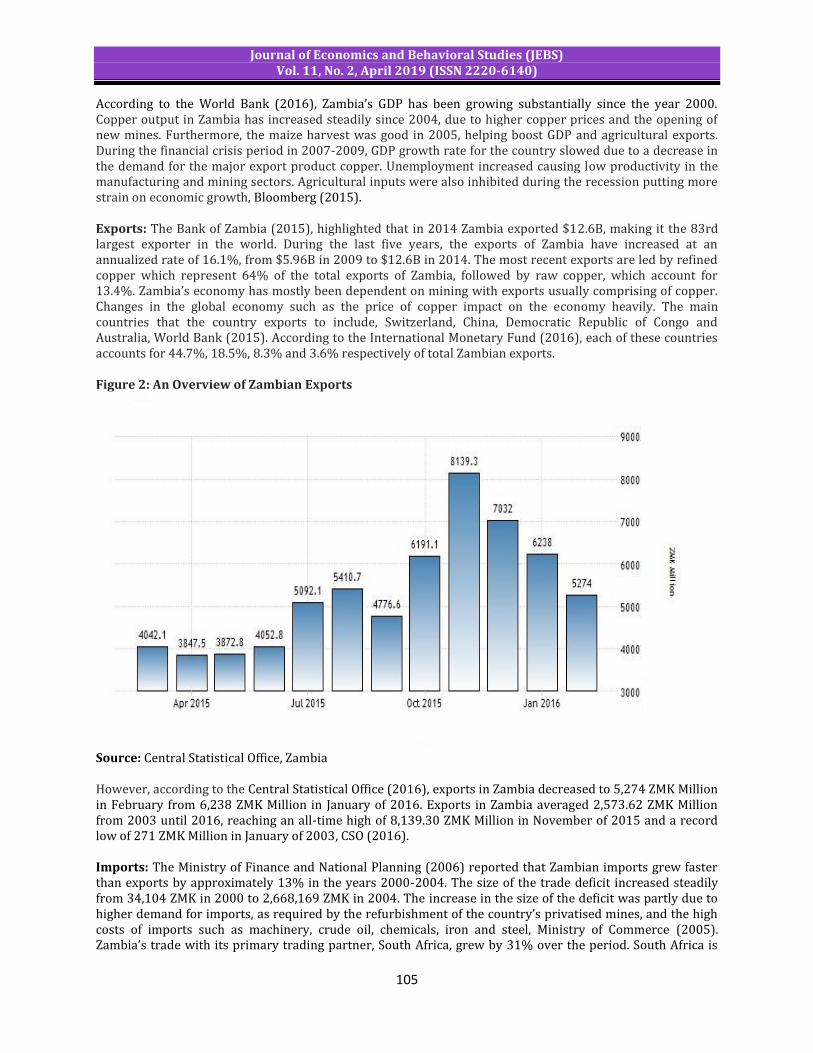
Journal of Economics and Behavioral Studies (JEBS) Vol. 11, No. 2, April 2019 (ISSN 2220-6140)
105
According to the World Bank (2016), Zambia’s GDP has been growing substantially since the year 2000. Copper output in Zambia has increased steadily since 2004, due to higher copper prices and the opening of new mines. Furthermore, the maize harvest was good in 2005, helping boost GDP and agricultural exports. During the financial crisis period in 2007-2009, GDP growth rate for the country slowed due to a decrease in the demand for the major export product copper. Unemployment increased causing low productivity in the manufacturing and mining sectors. Agricultural inputs were also inhibited during the recession putting more strain on economic growth, Bloomberg (2015). Exports: The Bank of Zambia (2015), highlighted that in 2014 Zambia exported $12.6B, making it the 83rd largest exporter in the world. During the last five years, the exports of Zambia have increased at an annualized rate of 16.1%, from $5.96B in 2009 to $12.6B in 2014. The most recent exports are led by refined copper which represent 64% of the total exports of Zambia, followed by raw copper, which account for 13.4%. Zambia’s economy has mostly been dependent on mining with exports usually comprising of copper. Changes in the global economy such as the price of copper impact on the economy heavily. The main countries that the country exports to include, Switzerland, China, Democratic Republic of Congo and Australia, World Bank (2015). According to the International Monetary Fund (2016), each of these countries accounts for 44.7%, 18.5%, 8.3% and 3.6% respectively of total Zambian exports. Figure 2: An Overview of Zambian Exports
Source: Central Statistical Office, Zambia However, according to the Central Statistical Office (2016), exports in Zambia decreased to 5,274 ZMK Million in February from 6,238 ZMK Million in January of 2016. Exports in Zambia averaged 2,573.62 ZMK Million from 2003 until 2016, reaching an all-time high of 8,139.30 ZMK Million in November of 2015 and a record low of 271 ZMK Million in January of 2003, CSO (2016). Imports: The Ministry of Finance and National Planning (2006) reported that Zambian imports grew faster than exports by approximately 13% in the years 2000-2004. The size of the trade deficit increased steadily from 34,104 ZMK in 2000 to 2,668,169 ZMK in 2004. The increase in the size of the deficit was partly due to higher demand for imports, as required by the refurbishment of the country’s privatised mines, and the high costs of imports such as machinery, crude oil, chemicals, iron and steel, Ministry of Commerce (2005). Zambia’s trade with its primary trading partner, South Africa, grew by 31% over the period. South Africa is
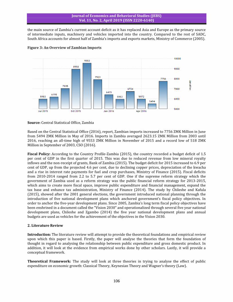
Journal of Economics and Behavioral Studies (JEBS) Vol. 11, No. 2, April 2019 (ISSN 2220-6140)
106
the main source of Zambia's current account deficit as it has replaced Asia and Europe as the primary source of intermediate inputs, machinery and vehicles imported into the country. Compared to the rest of SADC, South Africa accounts for almost half of Zambia’s imports and exports markets, Ministry of Commerce (2005). Figure 3: An Overview of Zambian Imports
Source: Central Statistical Office, Zambia Based on the Central Statistical Office (2016), report, Zambian imports increased to 7756 ZMK Million in June from 5494 ZMK Million in May of 2016. Imports in Zambia averaged 2623.15 ZMK Million from 2003 until 2016, reaching an all-time high of 9553 ZMK Million in November of 2015 and a record low of 518 ZMK Million in September of 2003, CSO (2016). Fiscal Policy: According to the Country Profile-Zambia (2015), the country recorded a budget deficit of 1.5 per cent of GDP in the first quarter of 2015. This was due to reduced revenue from low mineral royalty inflows and the non-receipt of grants, Bank of Zambia (2015). The budget deficit for 2015 increased to 6.9 per cent of GDP, up from the projected 4.6 per cent, due to declining copper prices, depreciation of the kwacha and a rise in interest rate payments for fuel and crop purchases, Ministry of Finance (2015). Fiscal deficits from 2010-2014 ranged from 2.2 to 5.7 per cent of GDP. One if the supreme reform strategy which the government of Zambia used as a reform strategy was the public financial reform strategy for 2013-2015, which aims to create more fiscal space, improve public expenditure and financial management, expand the tax base and enhance tax administration, Ministry of Finance (2014). The study by Chileshe and Kafula (2015), showed after the 2001 general elections, the government introduced national planning through the introduction of five national development plans which anchored government’s fiscal policy objectives. In order to anchor the five-year development plans. Since 2005, Zambia’s long term fiscal policy objectives have been enshrined in a document called the "Vision 2030” and operationalized through several five year national development plans, Chileshe and Zgambo (2014) the five year national development plans and annual budgets are used as vehicles for the achievement of the objectives in the Vision 2030. 2. Literature Review Introduction: The literature review will attempt to provide the theoretical foundations and empirical review upon which this paper is based. Firstly, the paper will analyse the theories that form the foundation of thought in regard to analysing the relationship between public expenditure and gross domestic product. In addition, it will look at the evidence from empirical works done by other scholars. Lastly, it will provide a conceptual framework. Theoretical Framework: The study will look at three theories in trying to analyse the effect of public expenditure on economic growth: Classical Theory, Keynesian Theory and Wagner’s theory (Law).
Journal of Economics and Behavioral Studies (JEBS) Vol. 11, No. 2, April 2019 (ISSN 2220-6140)
107
Keynesian Theory: Following the 1929-30 Great Depression, the classical economic argument for governments’ minimal level of involvement in the economy did not seem to hold. This brought about the development of Keynesian economics which is an economic theory of total spending in the economy and its effects on output and inflation. Keynesian economics was developed by the British economist John Maynard Keynes during the 1930s in an attempt to understand the Great Depression. Keynes advocated for increased government expenditures and lower taxes to stimulate demand. Keynes believed that when governments increase public spending, it gives individuals’ purchasing power and producers will produce more, creating more employment and overall output. This is the multiplier effect that shows causality from public expenditure to national income. However, it should be noted that Keynes developed this theory during depression and therefore, the conditions that were prevailing at that point were such that logical economic principles were not holding. Keynes equally acknowledged that government intervention was necessary as a short term cure and in the long-run, the economy should have minimal government intervention. Wagner’s Theory: Wagner (1883) predicted that economic growth would be accompanied by an increase in state activity (growth of government spending). A formulation of Wagner’s “law”, mentioned by Bird (1971), might run as follows: as per capita income rises in industrializing nations, their public sectors will grow in relative importance. Thus, the causality according to Wagner’s law is running from economic growth to government spending. Further, Wagner’s hypothesis emphasizes that, in the process of economic development, government economic activity increases relative to private economic activity. Wagner offers three reasons why this would be the case. Firstly, with economic growth industrialization and modernization would take place, which will diminish the role of public sector for private one. Secondly, the rise in real income would lead to more demand for basic infrastructure particularly education and health facilities. Wagner asserts, “it is the government who provide these facilities more efficiently than private sector". Thirdly, to remove monopolistic tendencies in the country and to enhance economic efficiency in those sectors where large amounts of investment are required, government should come forward and invest in those particular areas that will again increase public expenditure (Bird, 1971). Empirical Review: There was little empirical literature available on public expenditure prior to post-era 1929-30 Great Depression where economies underwent rising public expenditure. Subsequently, the post-war economic reconstruction and public welfare programmes become an interesting subject area for many economists to understand the effect of public expenditure on economic growth. This required a rigorous theoretical approach to public expenditure to be developed. It should be noted that empirical results have shown contrasting results on the effects of government expenditure on gross domestic product. Balaj and Lani (2017) analysed the Impact of Public Expenditure on Economic Growth of Kosovo. Their econometric model was built on two economic theories, Wagner and Keynesian. The results obtained from their study showed that there is a positive relationship between public expenditure and economic growth. However, their findings revealed that public expenditure does not have a direct impact on economic growth, but can have a stimulating effect on the economic growth process. Garba and Abdullahi (2013) investigated the causal relationship between public expenditure and economic growth in Nigeria and used Johansen co-integration approach and the Granger causality test. Their results indicated a significant long-run positive relationship between public expenditure and economic growth in Nigeria. Their study also found that there is a positive long-term relationship between population growth rate and economic growth. Katrakilidis and Tsaliki (2009) examined the relationship between spending and economic growth by using annual data of the Greek economy during the period 1958-2004. They applied recent developments in the theory of cointegrated processes (ARDL) and obtained empirical results indicating that the causality runs from income to government expenditures, which is in accordance with Wagner’s law. Conversely, they found that causality runs from expenditures to income, which supports the Keynesian hypothesis and claims that their study brought new evidence of two-directional causality between expenditures and income for the case of Greece. Akitoby et al. (2006) examined the short- and long-term behaviour of government spending with respect to output in 51 developing countries using an error-correction model. They find evidence that is consistent with the existence of cyclical racketing and voracity in government spending in developing countries, resulting in a tendency for government spending to rise over time.

Journal of Economics and Behavioral Studies (JEBS) Vol. 11, No. 2, April 2019 (ISSN 2220-6140)
108
Conceptual Framework Independent Variables Dependent Variables 3. Methodology The study applies an Autoregressive Distributed Lag (ARDL) model to analyse time series data spanning a period of 1980 – 2017. The data comprises yearly Zambian data for GDP growth rate, Government expenditure, Foreign Direct Investment (FDI) and the Current Account Balance (CAB). The data was retrieved from the United Nations Conference on Trade and Development (UNCTAD) and International Food Policy Research Institute (IFPRI) databases. The aim is to understand the behaviour of changes in public spending, with other control variables based on the Keynesian model, on Gross Domestic Product (GDP) both in the long run and short run. The model specification is stipulated as follows: (1)
(2)
Where: GDPr = Gross Domestic Product growth rate GOVT exp= Government Expenditure FDI= Foreign Direct Investment CAB = Current Account Balance K = is the maximum lag of a regressor in the model β = Parameters ε = error term From the ARDL model above, a long run model and short-run model (Error Correction Model) was estimated. This is on the basis of the Bounds test showing existence of a long run relationship. This approach is much easier than the Johansen cointegration as it uses a single equation approach and can, therefore, be used on smaller sample sizes. The long run and short run model are specified in equation 3 and 4 respectively below;
(3) Where: ECT = Error Correction Term All other variables are defined as before (4)
To ensure reliable estimators, the ARDL model was subjected to diagnostic testing. These included the Breusch-Pagan test for autocorrelation and Whites Heteroscedasticity test for heteroscedasticity testing. The Jarque-Bera was used to test for normality of the residuals and finally a Cusam test to ensure stability of the model.
Government expenditure
Foreign Direct Investment
Current Account Balance
Gross Domestic Product

Journal of Economics and Behavioral Studies (JEBS) Vol. 11, No. 2, April 2019 (ISSN 2220-6140)
109
4. Results and Discussion Table 1: Unit Root Tests Variable ADF KPSS Summary
Statistic at Level (p-value)
Result Statistic at level (5% critical value)
Result
GDP -5.19936* (0.0008)
I(0) 0.105 (0.146)
I(0) I(0)
Government Exp (Govt_x)
-5.11233* (0.0010)
I(0) 0.095 (0.146)
I(0) I(0)
FDI -4.824* (0.0022)
I(0) 0.119771 (0.146)
I(0) I(0)
Current Account Balance (CAB)
-2.118725* (0.00344)
I(0) 0.457 (O.463)
I(0) I(0)
Note: I (1), indicates a unit root at levels and stationarity after first difference *denotes significant at 5% level and the rejection of the null hypothesis The results in Table 1 show that all the variables of interest are stationary at levels. The ADF test was able to reject each null hypothesis of no stationary at 5% as observed from the p-values. Similarly, the KPSS was unable to reject any of the null hypotheses of stationary as KPSS statistic observed to be lower than the 5% critical value. To allow for a long run and short run estimation, the ARDL model was used. To ensure the viability of this model, the bounds cointegration test is first presented. Table 2: ARDL Bounds Test F statistic 5.2748713 Critical values I0 I1
10% 2.97 3.74
5% 3.38 4.23
1% 4.3 5.23
The Bounds test in Table 2 indicates the presence of cointegration as expected. The F-statistic is greater than the upper bound at 10%, 5% and 1% indicating that the null hypothesis of no long-run relationship is rejected. Having verified the existence of a long run relationship between the dependent and independent variable, the long run model is shown below in Table 3. Table 3: Long Run Model Variable Coefficient T-statistic P-value Govt_Exp -0.94422* -2.594272 0.0183 FDI 1.657286 1.591175 0.1290 CAB -0.116239 -0.834115 0.4151 Trend -0.276561 -1.242937 0.2298 * denotes the statistically significant coefficients Table 3 indicates that only government expenditure has a significant impact on the growth rate in the long run. However, this impact is noted to be negative which may be contrary to expectations and to previous studies such as Muyaba (2016). This also goes against the Keynesian theory that suggests increased government expenditure will have a positive impact on economic growth. Foreign direct investment has a positive impact as expected whilst the current account balance has a contrary, negative impact. However, both FDI and the current account do not have a significant impact on economic growth in the long run. The R-squared showed how well the model fits it’s the data, specifically, 89% of changes in economic growth are

Journal of Economics and Behavioral Studies (JEBS) Vol. 11, No. 2, April 2019 (ISSN 2220-6140)
110
explained by explanatory variables. To get a picture of changes in GDP in the short run, the Error correction model is estimated in Table 4 below. Table 4: Short Run Model Variable Coefficient T-statistic P-value ECT(-1) -0.519067* -5.677616 0.0000 D(GDP(-1)) -0.554758* -4.313223 0.0004 D(GDP(-2)) -0.305082* -2.319577 0.0323 D(GDP(-3)) -0.269714* -2.813015 0.0115 D(Govt_exp) -0.169750* -3.636914 0.0019 D(Govt_exp(-1)) 0.177382* 3.031643 0.0072 D(Govt_exp(-2)) 0.150246* 2.545659 0.0203 D(FDI) 0.37185* 2.089709 0.0511 D(FDI(-1)) -0.634135* -3.288530 0.0041 D(FDI(-2)) -0.576605* -3.327873 0.0037 D(CAB) 0.128317* 2.443381 0.0251 C -0.519067* -5.677616 0.0000 R-squared = 0.908318 F-statistic (p-value) = 0.00000 *D indicates a differenced variables, ECT indicates the Error Correction Term and C, the intercept term. The short run model indicates that all the variables of interest have a statistically significant impact on the economic growth rate of Zambia. Government expenditure in the short run, as in the long run, has a negative impact on the economy contrary to expectations. FDI, on the other hand, has a positive impact on Zambia’s economy in the short run. This is expected as investors will upon investing pump money into the economy, employ several citizens and among other things, create an environment for other businesses to grow, inevitably increasing output in the short run. The current account balance has a positive impact on the economy of Zambia as a surplus inevitably indicates increases output as it suggests increased exports over imports. This may be related to the impact of FDI as increased investment will increase CAB also in the short run. Generally, the short run model also reflects a good fit with the explanatory variables explaining 90.8% of changes in the growth rate. This R-squared value is also statistically significant as the F Statistic has a very low p-value. The Error correction term (ECT) reemphasizes the existence of a long run relationship due to negative coefficient and it’s statically significance. The term has a value of -0.51907 indicating that 51.9% of disequilibrium in the short run is adjusted towards the long run equilibrium within a year. Diagnostic test for autocorrelation, heteroscedasticity, model stability and normality of residuals is shown in the Appendix. 5. Conclusion Zambia experienced a significant increase in GDP growth after it gained independence. The main contributor to this increase was the boom in mining which is the hub of the country with copper reserves being amongst the top in the world. Exports of copper increased and impacted positively on GDP growth and reduced inflation the movement for multi-party democracy however decided to privatise a large portion of the mines after 1991 to foreign investors. The move was applauded by some financial players and it helped Zambia reach the heavily indebted poor countries (HIPC) completion point. This move enabled the International Monetary Fund and World Bank to cancel the remaining debt which the country owed. The social status of people was uplifted as the government could now channel money to other projects in the country for development. However, in the past 6 years, Zambia has experienced setbacks in its economic performance. Fiscal deficit has increased and the low prices of copper on the London Stock Exchange have contributed to the poor economic performance of the country. Cointegration results show that there is a long run relationship between GDP and government expenditure. In this regard, changes in government expenditure have a strong converse effect on GDP. Government expenditure, which has increased significantly in the past decade, is seen to have had negative effects both in the short run and long run. Contrary to theory, increased government expenditure may not be ideal for growing the Zambian economy. This could be due to the allocation of this public expenditure, i.e. the 2018 Budget had 24% of the expenditure directed to economic activities. Thus it is recommended that
Journal of Economics and Behavioral Studies (JEBS) Vol. 11, No. 2, April 2019 (ISSN 2220-6140)
111
government practice increased fiscal discipline or reallocated resources as their expansionary fiscal policies are not yielding the intended results. Additionally, policies to promote private investment may be more beneficial for the Zambian economy. On the other hand, increased investment is recommended that government also encourage more investment promoting policies as FDI is observed to have a positive impact in the short run though insignificant in the long run. These should ensure more investors are encouraged to stay longer and the impacts /externalities of their investments be accrued to the nationals to ensure long-run benefits. The Zambian government should also ensure that the country diversifies its export base and enhances its external debt management to ensure positive and consistent impact of CAB in the long run. References Akitoby, B. (2006). Public spending, voracity, and Wagner’s Law in developing countries. European Journal of
Political Economy, 22, 908-924. African Development Bank Group. (2014). Zambia Economic Outlook. Bank of Zambia. (2006). Bank of Zambia Monetary Policy Statement: January to June 2006. Lusaka, Zambia Bank of Zambia. (2015). Monetary Policy Statement, May 2015, Lusaka. Bank of Zambia. (2016). Zambia Direction of Trade Report. Balaj, D. & Lani, L. (2017). The Impact of Public Expenditure on Economic Growth of Kosovo. ACTA
UNIVERSITATIS DANUBIUS, 13(5), 401-412. Bird, R. (1971). Wagner’s Law of Expanding State Activity. Public Finance, 26(1), 1283-91. Chileshe, M. P. & Kafula, L. (2015). The effects of fiscal policy on the conduct and transmission mechanism of
monetary policy in Zambia. A report prepared for the COMESA Monetary Institute. Chileshe, M. P. & Zgambo, P. (2014). An empirical investigation of the effectiveness of monetary policy in
Zambia. A study commissioned by the COMESA Monetary Institute. Country Profile-Zambia. (2015). United Nations Economic Commission for Africa, Addis Ababa, Ethiopia Fagernas, S. & Roberts, J. (2004). The Fiscal Effects of Aid in Zambia, ESAU Working Paper 10, Overseas
Development Institute, London Garba, T. & Abdullahi, S. Y. (2013). Public expenditure and economic growth; An application of co-integration
and Granger causality test on Nigeria. Journal of Economics and Social Research, 15(1), 1–30. Gnynne, R. (1996). Trade and Developing Countries: The Global Economy in Transition, Longman, Essex Johansen, S. & Juselius, K. (1990). Maximum Likelihood Estimation and Inference on Cointegration – with
Applications to the Demand for Money, Oxford Bulletin of Economics and Statistics, 52(2), 169-210. Katrakilidis, C. & Tsaliki, P. (2009). Further evidence of causal relationship between government spending
and economic growth: the case of Greece, 1958-2004. Acta Economica, 59(1), 57-78 Ministry of Commerce. (2005). Zambia Diagnostic Trade Integration Study, World Bank Sponsored Study.
http://www.integratedframeworking.org/countries/zambia.htm Ministry of Finance and National Planning. (2005). Economic Report 2004. Lusaka, Zambia Ministry of Finance and National Planning. (2006). Economic Report 2005. Lusaka, Zambia Ministry of Finance. (2014). 2015 National Budget Speech, Lusaka Muyaba, A. M. (2016). Public Spending and Economic growth in Zambia. An Econometric Analysis. Cape
Town: University of Cape Town. Rakner, L. (2003). Political and Economic Liberalization in Zambia 1999-2001, Nordic Africa Institute,
Uppsala Republic of Zambia. (2000). Interim Poverty Reduction Strategy Paper, www.imf.org Turok, B. (1989). Mixed Economy in Focus: Zambia, London Institute of African Alternatives Osei-Hwedie, B. Z. (2003). Development Policy and Economic Change in Zambia: A Re-Assessment, DPMN
Bulletin: Vol. X Number 2. Wagner, A. (1883). Finanzwissenschaft. Leipzig. Wagner, A. (1911). Staat in nationalökonomischer Hinsicht. In Handwörterbuch der Staatswissenschaften.
Third edition, Book VII. Jena: Lexis, 743–745. World Bank. (2003). Zambia: Public Expenditure Management and Financial Accountability Review, Country
Financial Accountability Annex, Vol. II, Report No. 26162-ZA, Washington DC World Bank. (2016). Zambia Economy, http:www.zambia-invest.com/economy World Bank. (2015). Zambia Country Programme Evaluation, FY04-13: Independent Evaluation, International
Bank for reconciliation and Development.

Journal of Economics and Behavioral Studies (JEBS) Vol. 11, No. 2, April 2019 (ISSN 2220-6140)
112
Revenue Productivity of the Tax System in Namibia: Tax Buoyancy Estimation Approach
J P S Sheefeni10, A Shikongo2, O Kakujaha-Matundu2, T Kaulihowa2 1Department of Economics, University of the Western Cape South Africa, South Africa
2Department of Economics, University of Namibia, Namibia [email protected]
Abstract: Buoyancy refers to how tax revenue responds to a gross domestic product without correcting for discretionary alterations in the tax system. The paper assessed the buoyancy of Namibia’s overall tax system in an attempt to measure the response of the tax system in entirety because of fluctuations in the national income and/or the deliberate act by the government to increase tax rate, reviewed tax code and tax machinery etc. The study employed the Engle-Granger approach to the error correction model to estimate the tax buoyancy for the period 2001 to 2014. The empirical findings from the study revealed that overall the Namibian tax system is income inelastic and not buoyant. This is confirmed by a low and negative value of 0.036 which is less than unit. Thus, the economy is not generating sufficient revenue both through discretionary tax measure and through the expansion in the economic activities. Therefore, the government need to introduce measures that will allow for more tax revenue collection to have a stable revenue base. This also means the government need to keep track of tax mobilization with growth in the gross domestic product as well as to ascertain taxes that are productive. Keywords: Government expenditure, tax buoyancy, tax revenue, income inelastic, gross domestic product
1. Introduction Taxation generates most income for government in Namibia with the contribution of 65% towards the total revenue (Bank of Namibia [BoN], 2015). According to this report, Namibia is experiencing persistent increase in government expenditures and a drop in government revenue. Thus, like other developing countries Namibian government is faced with challenges of mobilising enough resources to finance capital projects, poverty alleviation and to attain the targets stated by government in the national development plans. With current reduction in donor funding, the global economic crises and reduction in SACU revenue, Namibia is left with no option but to mobilise more revenue domestically in order to avail the much-needed funds for developmental projects and to address socio-economic challenges facing the country. Namibia gained independence on 21 March 1990. Prior to independence, Namibia has been using the tax system of the colonial masters of the time. Namibia’s post-independence tax system operation was still under the tax system that was inherited from colonial government until amendments and changes were made some years later. Particularly, the Namibian tax system is regulated by the Income Tax Act and Value Added Tax Act 10 of 2000. Employee tax is another tax head collected by the employer from the employee and remitted to the Receiver of Revenue. These taxes are collected and enforced by the Department of Inland Revenue and Customs in the Ministry of Finance. Namibia has a source-based tax system which implies that Namibian residents and foreign nationals are liable to pay tax on the income generated in the country. Thus tax is imposed on taxable income of individual and corporate sourced within Namibia. It is for this reason, Bonga, Dhoro-Gwaendepi and Mawire-Van Strien (2015) defined tax as a fiscal load on economic agents such as individuals or property owners to support the government. The Namibian tax structure consists of two major direct taxes: individual income tax and corporate income tax and two main indirect taxes: Value Added Tax (VAT) and Value Added Tax on Imports. In Namibia, the Ministry of Finance is mandated by the constitution to manage public finance and state revenue, to control the government assets and liabilities and overseeing financial regulations, public finances and government revenues. Thus, the Namibian government had been pursuing a number of amendments over the years with the primary objective of designing a sustainable and productive system to fund and sustain the operations of the government without resorting to deficit financing. Post-independence, the main sources of tax revenue have been a share from Southern African Customs Union (SACU), Income tax on individuals and the mining sector and general sales tax which was only operational from independence to
10
Corresponding author

Journal of Economics and Behavioral Studies (JEBS) Vol. 11, No. 2, April 2019 (ISSN 2220-6140)
113
2000. According to the report by the Bank of Namibia (2016), SACU revenue has been one of the major contributors to the overall tax revenue up to some few years back. However, the situation changed when global economic and financial crises took effect. This resulted in a SACU share drop to 3 billion from 8 billion Rand. Tax from sales had been the second main contributor to total tax revenue followed by income tax in the first decade after the independence. Analysis of the medium-term expenditure framework (MTEF) or rolling budget shows that between 2011 and 2014 total revenue increased progressively from N$ 20.7 billion in 2007 to N$ 24.2 billion in 2010. This was attributed to greater revenue from SACU common revenue pool and revenue enhancing policy, driven by enhanced revenue collection and improved tax administration. Namibia has achieved a commendable tax to gross domestic product revenue collection ratio, which averages 34.3 percent in recent years, as seen against the global average of about 16.2 percent. In exclusion of SACU revenue, the national (Namibia) tax to GDP ratio stood at an average of 23.2 percent, which can be compared to the rest of the world (BoN, 2015). Namibian government debt to GDP which measures the country’s ability to pay its debt has a direct effect on the cost borrowing and the bond yields. According to BoN (2016) on average government debt to GDP had been 20.88 percent between 1993 and 2015 with the ever high recorded debt to GDP of 34 percent in the last quarter of 2015. This literary means that the government had not been mobilising sufficient resources to fund the ever-increasing government expenditure. Therefore, this study examined whether or not government is generating sufficient revenue through discretionary tax measure and/or the expansion in the economic activities. This study is the first of its kind in Namibia and shed some light on the subject matter. More so, it adds on Namibia’s empirical literature on this specific subject. 2. Literature Review Economists have developed a number of theories of taxation over time to guide governments on how to harness the tax system in response to mitigate the persistence of fiscal imbalances. Singer (1968) measured or estimated tax buoyancy by estimating aggregate tax based revenue on Gross Domestic Product (GDP), which is proxy for the tax base and incorporating a dummy variable. Osoro (1993) defined tax buoyancy as the ratio of change as in growth in tax revenue to a change as in growth in the tax base. Therefore, it can be concluded that tax buoyancy measures the change in tax income (revenue) due to changes in national income without controlling for discretionary change in tax policy. Similarly, Mukarram (2001) defined buoyancy as tax revenue responsiveness to GDP without correcting for discretionary alterations in the tax system. It attempts to measure the overall response of the tax system resulting from both variations in the national income as well as discretionary act by government to raise tax rate, reviewed tax code and tax machinery etc. Tax Buoyancy = %∆T/%∆GDP. Where, ∆T is the change in tax revenue and ∆GDP, change in GDP. GDP is taken as base, although it is possible to have other bases. Several studies have used GDP as one of the determinants of tax revenue. There are numerous studies that have empirically estimated the tax buoyancy, varying from different parts of the world. Among the authors who conducted empirical work on the subject matter are as presented below. Wanjiku (1993) examined the productivity of revenue’s implications of the tax system and that of individual taxes in Kenya over the period from 1972/73 to 1990/90. A proportional adjustment method (PAM) and a double log regression function were employed to estimate tax buoyancy and tax elasticity. The results showed an inelastic tax system with respect to income with a value of 0.67064. The performance of the income taxes was not statistically significant, though showed a slight improvement with an elasticity of 1.07130. Similarly, in Ghana, Kusi (1998) also employed a proportional adjustment method on data covering the period 1983 to 1993. In addition, the study also utilised a constant rate structure to estimate the tax buoyancy and tax elasticity. This was to assess how productive the overall tax system is as well as that of the individual tax heads. The results from this study revealed that post-reform buoyancy of (1.29) and elasticity (1.22) was much larger than the pre-reform period of (0.72) and (0.71) buoyancy and elasticity respectively. The study revealed a major impact on both. Particularly, the study attributed low buoyancy and elasticity during the pre-reform period to smuggling, unrecorded trade, tax evasion and laxity in tax collection. Another study on the same subject but in a different continent by Mukarram (2001) examined the elasticity and buoyancy in Pakistan, specifically for the major taxes covering the period 1981-2001. Using the chain indexing technique, the results reveal that the tax estimates were higher for direct taxes, followed by those of

Journal of Economics and Behavioral Studies (JEBS) Vol. 11, No. 2, April 2019 (ISSN 2220-6140)
114
sales taxes. The results further indicated that customs and excise duties are rigid as a result of tax elasticity which was low. The study concluded that higher buoyancy estimates in comparison with coefficient estimates of elasticity for all the taxes confirm that growth in revenue was achieved due better tax rates and widened tax base as an alternative to automatic growth. On the same country, Bilquees (2004) applied a divisia index approach examined the elasticity and buoyancy of the tax system in Pakistan over the period 1974/5 to 2003/4. The results from this study indicated that elasticity coefficient of the tax revenue both with respect to total GDP and non-agricultural GDP is less than a unit. The buoyancy estimates suggested that tax restructuring was less impactful in realising revenue growth in Pakistan. In the Southern African region, Bolthole and Aglobenebo (2006) conducted a study on Botswana to estimate both tax elasticity and tax buoyancy. In employing the vector error correction model (VECM), the results revealed that the tax system was income inelastic but buoyant. Tax buoyancy results were also found by the results of a study by Timsina (2007) in Nepal. In particular, the results of the study showed that the tax system in Nepal was less responsive (inelastic). However, the buoyancy coefficient was more than unitary, suggesting that most revenue collections emanates from discretionary policy in the tax policy and not form self-adjusting. Tegegn (2008) assessed the tax revenue productivity in Ethiopia for the period 1961 to 2005. Using a dummy variable technique approach, the results showed that tax revenue tends to be inelastic with respect to change in the tax base. Using a similar approach, Twerefou, Fumey, Assibey and Asmah (2010) conducted the same study in Ghana. Particularly, the authors used the historical time series data for the period 1970 – 2007. In employing the residual approach to cointegration for long-run analysis, the results revealed that the overall tax system was buoyant and responsive, though the opposing results were evident in the short-run. Gituku (2011) employed the proportional adjustment method (PAM) which was also used by Samwel and Isaacs (2012) to estimate elasticity and buoyancy of the various tax components employing this method on Kenyan data for the period of 24 years. The findings of this study revealed an inelastic tax with respect to income. In Zimbabwe, Ndedzu, Macheka, Ithiel and Zivengwa (2013) evaluated Zimbabwe’s revenue productivity of overall tax system covering 1975 to 2008. They employed a dummy variable technique to compute buoyancy. Their results were not buoyant with the overall tax systems except customs duty. The study concluded that buoyant and elastic tax structure is the most appropriate in a developing country. This means an automatic adjustment of tax collection in tandem with growth in national income, hence less discretionary changes. In Kenya, Mawia and Nzomoi (2013) examined tax buoyancy using quarterly data for the period 1999/2000 - 2010/2011. The findings revealed an overall buoyant tax system with a value of 2.58, while their individual tax heads were not buoyant with the exception of excise duties which was found buoyant with respect to the base. The study noted that the responses of tax bases to changes in economic activities showed high buoyant values greater than unit. Similarly, Meshak (2014) evaluated the Nigerian’s tax productivity. The data used was that of GDP and aggregate tax revenue covering 1993 to 2012. The study adopted tax buoyancy as against elasticity in the decomposition process of tax-to-base and base-to-income. The results showed that two out of four tax bases has a buoyancy above a unit with VAT as the most buoyant of all with the coefficient of 1.82, while the total tax revenue has the buoyancy of 0.95. Mandela and Olukuru (2015) assessed the extent of tax buoyancy in Kenya between the year 1980 to 2014 and also of South Africa between the years 1972 to 2014. The study adopted the error correction modelling approach for this purpose. The results revealed that tax system for both countries is buoyant, both in the short run and long run. Particularly, the study found a statistical significant buoyancy coefficient of 1.77 for South Africa and 1.18 for Kenya in the long run respectively. Results ofshort-run buoyancy coefficients showed a significant 1.82 and 2.69 for South Africa and Kenya respectively. Edeme, Nkalu, Azu and Nwachucku (2016) examined the relationship between tax revenue and Gross Domestic Product in Nigeria for the period 1970 to 2013. The study employed an ordinary least squares in the form of log-linear to compute the buoyancy estimates. The findings of the study indicated that tax revenue is highly buoyancy with respect to national income. The study also found a very low buoyant coefficient in response to revenue from the social sector. The theoretical and empirical literature showed numerous methods used to analyse the productivity of the tax system in different countries. This includes among others Dummy Variable Approach, Divisia Index method, Constant Rate Structure, Proportional Adjustment Method, Ordinary Least Squares, Error Correction Models and Vector Error Correction Models. In terms of findings, there seem to be mixed
Journal of Economics and Behavioral Studies (JEBS) Vol. 11, No. 2, April 2019 (ISSN 2220-6140)
115
findings from positive to negative effect, elastic buoyancy to inelastic buoyancy. In the absence of an empirical study of this nature in Namibia, this study intends to be the first of its kind to shed some light and fill this gap. 3. Methodology The section constitutes three sub-sections. Section one presents the analytical framework. The second sub-section discusses the model construction and specification. Lastly, sub-section three discusses data issues and the measurement of variables. Analytical Framework: It is well known that as time changes government undertakes changes in the form of change in tax rates, tax reforms and budget rationalization programmes. These changes are aimed at enhancing and harnessing revenue productivity of the tax system in response to the dynamics of the economy. Therefore, studying the productivity of the tax system is essential especially, particularly this study utilised the approach of Singer (1968) to analyse tax buoyancy. Tax Buoyancy: Tax Buoyancy is a measure of percentage change in tax revenue, including discretionary tax changes due to a percentage change in GDP which is the base (Bonga et al., 2015). Tax buoyancy outlines the connection between the change in state’s tax revenue growth and the change in national income. Tax buoyancy can be evaluated by regressing tax revenue over the tax base which is real GDP in this case once applying the natural logarithm for each of them. This assesses the link between the proportional changes in revenue and those in GDP. To measure the overall buoyancy of the tax system, the relative change in total revenue from tax with respect to the relative change in national income. This is stated as:
=
(1)
From the above expression T is total tax revenue, Y represents GDP. The buoyancy of the tax system can be decomposed into buoyancy of individual taxes;
=
+
+ … + =
(2)
= + + … + and n is the number of tax heads. Buoyancy of the tax system according to Bonga et al. (2015) it is the weighted sum of individual tax head buoyancy and this is utilised to acquire elasticity of tax with respect to tax-to-base and base-to-income stated as:
Tax - to – base – elasticity =
(3)
And
Base – to – income – elasticity =
(4)
Buoyancy of the tax system than becomes;
=
=
(5)
Tax buoyancy is measured in the way with tax elasticity. According to Appiah (2013) the only difference is when discretionary measures are not controlled which change the tax rate and/or base, then the sensitivity of tax revenue to changes in national income is the buoyancy. This means that a tax is buoyant when the value is greater than unit/one. In cases where the elasticity of main revenue bases are low irrespective of the amendments and incentives that the state undertakes due to factors such as evasion, the state resort to raising additional resources through discretionary measures. Tax revenue increases when the buoyancy is high compared to elasticity. Model Specification and Data Analysis: This study will follow the unadjusted historical time series tax data with the dummy variables integrated as proxies for discretionary tax measures as developed by Singer (1968) to measure buoyancy and elasticity of the tax system, because of non-intensive data required and for the fact that it does not require disaggregated data. By specifying Singer’s (1968) multiplicative form of a tax revenue model stated as: TTR = lnTTR = α + βlnGDP + z (6) Ordinary Least Square (OLS) is applied to equation (6) to estimate the parameters α and β, the coefficient β represent the tax buoyancy estimates and z it the stochastic term. Y in the Singer’s equation represents GDP. Using equation (6) above tax buoyancy is decomposed in two components:
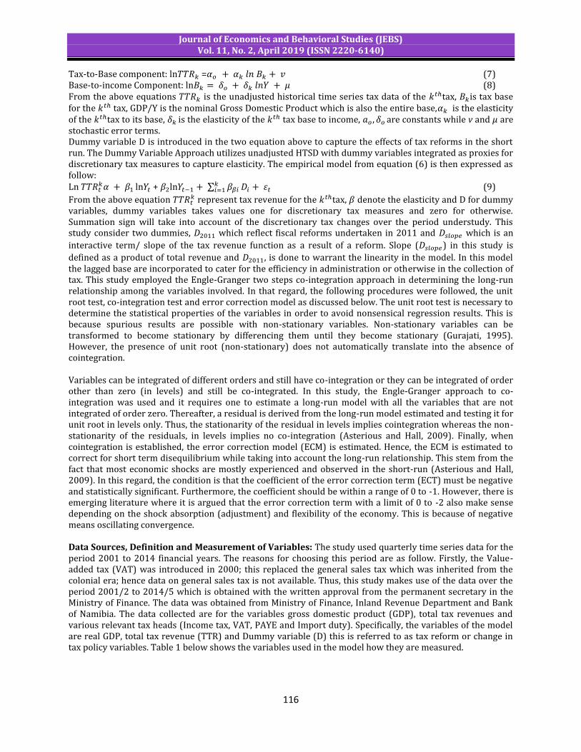
Journal of Economics and Behavioral Studies (JEBS) Vol. 11, No. 2, April 2019 (ISSN 2220-6140)
116
Tax-to-Base component: ln = (7) Base-to-income Component: ln (8) From the above equations is the unadjusted historical time series tax data of the tax, is tax base for the tax, GDP/Y is the nominal Gross Domestic Product which is also the entire base, is the elasticity of the tax to its base, is the elasticity of the tax base to income, are constants while v and are stochastic error terms. Dummy variable D is introduced in the two equation above to capture the effects of tax reforms in the short run. The Dummy Variable Approach utilizes unadjusted HTSD with dummy variables integrated as proxies for discretionary tax measures to capture elasticity. The empirical model from equation (6) is then expressed as follow: Ln
ln + ln (9)
From the above equation represent tax revenue for the tax, denote the elasticity and D for dummy
variables, dummy variables takes values one for discretionary tax measures and zero for otherwise. Summation sign will take into account of the discretionary tax changes over the period understudy. This study consider two dummies, which reflect fiscal reforms undertaken in 2011 and which is an
interactive term/ slope of the tax revenue function as a result of a reform. Slope ( ) in this study is
defined as a product of total revenue and , is done to warrant the linearity in the model. In this model the lagged base are incorporated to cater for the efficiency in administration or otherwise in the collection of tax. This study employed the Engle-Granger two steps co-integration approach in determining the long-run relationship among the variables involved. In that regard, the following procedures were followed, the unit root test, co-integration test and error correction model as discussed below. The unit root test is necessary to determine the statistical properties of the variables in order to avoid nonsensical regression results. This is because spurious results are possible with non-stationary variables. Non-stationary variables can be transformed to become stationary by differencing them until they become stationary (Gurajati, 1995). However, the presence of unit root (non-stationary) does not automatically translate into the absence of cointegration. Variables can be integrated of different orders and still have co-integration or they can be integrated of order other than zero (in levels) and still be co-integrated. In this study, the Engle-Granger approach to co-integration was used and it requires one to estimate a long-run model with all the variables that are not integrated of order zero. Thereafter, a residual is derived from the long-run model estimated and testing it for unit root in levels only. Thus, the stationarity of the residual in levels implies cointegration whereas the non-stationarity of the residuals, in levels implies no co-integration (Asterious and Hall, 2009). Finally, when cointegration is established, the error correction model (ECM) is estimated. Hence, the ECM is estimated to correct for short term disequilibrium while taking into account the long-run relationship. This stem from the fact that most economic shocks are mostly experienced and observed in the short-run (Asterious and Hall, 2009). In this regard, the condition is that the coefficient of the error correction term (ECT) must be negative and statistically significant. Furthermore, the coefficient should be within a range of 0 to -1. However, there is emerging literature where it is argued that the error correction term with a limit of 0 to -2 also make sense depending on the shock absorption (adjustment) and flexibility of the economy. This is because of negative means oscillating convergence. Data Sources, Definition and Measurement of Variables: The study used quarterly time series data for the period 2001 to 2014 financial years. The reasons for choosing this period are as follow. Firstly, the Value-added tax (VAT) was introduced in 2000; this replaced the general sales tax which was inherited from the colonial era; hence data on general sales tax is not available. Thus, this study makes use of the data over the period 2001/2 to 2014/5 which is obtained with the written approval from the permanent secretary in the Ministry of Finance. The data was obtained from Ministry of Finance, Inland Revenue Department and Bank of Namibia. The data collected are for the variables gross domestic product (GDP), total tax revenues and various relevant tax heads (Income tax, VAT, PAYE and Import duty). Specifically, the variables of the model are real GDP, total tax revenue (TTR) and Dummy variable (D) this is referred to as tax reform or change in tax policy variables. Table 1 below shows the variables used in the model how they are measured.

Journal of Economics and Behavioral Studies (JEBS) Vol. 11, No. 2, April 2019 (ISSN 2220-6140)
117
Table 1: Definition and Measurement of Variables Variable Definition and Measurement Total tax revenue (TTR) This is the total revenue of all individual tax heads and its measured in
Namibian dollars Gross Domestic Product (GDP)
This is the value of goods and services produced in a country over the period of one year irrespective of whether they were produced by foreigners or domestic residents. This is measured in Namibian dollar as well.
Dummy variable (D1) This is a slope dummy variable representing changes undertaken in 2011 and this takes 1 for the change and zero for otherwise.
4. Analysis and Discussion of Empirical Results This section presents the empirical findings and discussion. Firstly, the discussion is on the findings on the unit root test results. Secondly, the results for the cointegration test. Thirdly, the error correction model is also presented and discussed. The Unit Root Test: It is generally accepted that the first step to time series modelling should be testing the statistical properties of the data well known as the unit root test. In this study, the Augmented Dickey-Fuller test for unit root was used. Table 2: Unit Root Test: ADF in levels and First Difference Variable Model
specification Levels First Difference Order of
integration LNTTR Intercept -1.735 -8.148** I(1)
Trend and intercept -3.276 -8.255** I(1)
LNGDP Intercept -0.384 -2.937** I(1)
Trend and Intercept -2.897 -2.925** I(1)
LNETX Intercept -1.232 -8.401** I(1)
Trend and Intercept -2.315 -8.493** I(1)
LNITX Intercept -1.132 -7.573** I(1)
Trend and Intercept -2.611 -7.502** I(1)
Note: ** means the rejection of the null hypothesis at 5% Table 2 presents the results of the unit root test in levels as well as in first difference. The result shows that all the variables are nonstationary in levels. This suggests that the null hypothesis of non-stationarity of the variables could not be rejected in levels. Therefore, the variables were differenced once and eventually became stationary. Thus, all the variables are integrated of order one I(1). It follows that the basic ordinary least square cannot be directly applied to these variables due to the non-stationarity nature. Hence, the suitable modelling strategy to use was the Engle-Granger two-step procedures to estimate the regression model. Cointegration Test: The cointegration analysis was done by estimating Engle-Granger co-integration relationships better known as the residual based approach. The first step required an estimation of a long-run model from which the residual was derived. Table 3: Unit Root Test for the Residuals t-Statistic Prob.*
Augmented Dickey-Fuller test statistic -3.517033 0.0111
Test critical values: 1% level -3.555023
5% level -2.915522
10% level -2.595565
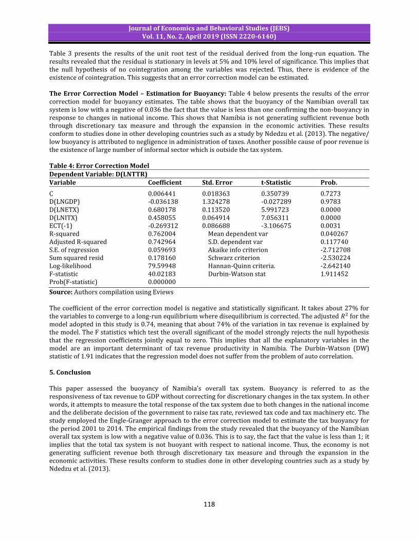
Journal of Economics and Behavioral Studies (JEBS) Vol. 11, No. 2, April 2019 (ISSN 2220-6140)
118
Table 3 presents the results of the unit root test of the residual derived from the long-run equation. The results revealed that the residual is stationary in levels at 5% and 10% level of significance. This implies that the null hypothesis of no cointegration among the variables was rejected. Thus, there is evidence of the existence of cointegration. This suggests that an error correction model can be estimated. The Error Correction Model – Estimation for Buoyancy: Table 4 below presents the results of the error correction model for buoyancy estimates. The table shows that the buoyancy of the Namibian overall tax system is low with a negative of 0.036 the fact that the value is less than one confirming the non-buoyancy in response to changes in national income. This shows that Namibia is not generating sufficient revenue both through discretionary tax measure and through the expansion in the economic activities. These results conform to studies done in other developing countries such as a study by Ndedzu et al. (2013). The negative/ low buoyancy is attributed to negligence in administration of taxes. Another possible cause of poor revenue is the existence of large number of informal sector which is outside the tax system. Table 4: Error Correction Model Dependent Variable: D(LNTTR) Variable Coefficient Std. Error t-Statistic Prob. C 0.006441 0.018363 0.350739 0.7273 D(LNGDP) -0.036138 1.324278 -0.027289 0.9783 D(LNETX) 0.680178 0.113520 5.991723 0.0000 D(LNITX) 0.458055 0.064914 7.056311 0.0000 ECT(-1) -0.269312 0.086688 -3.106675 0.0031 R-squared 0.762004 Mean dependent var 0.040267 Adjusted R-squared 0.742964 S.D. dependent var 0.117740 S.E. of regression 0.059693 Akaike info criterion -2.712708 Sum squared resid 0.178160 Schwarz criterion -2.530224 Log-likelihood 79.59948 Hannan-Quinn criteria. -2.642140 F-statistic 40.02183 Durbin-Watson stat 1.911452 Prob(F-statistic) 0.000000 Source: Authors compilation using Eviews The coefficient of the error correction model is negative and statistically significant. It takes about 27% for the variables to converge to a long-run equilibrium where disequilibrium is corrected. The adjusted for the model adopted in this study is 0.74, meaning that about 74% of the variation in tax revenue is explained by the model. The F statistics which test the overall significant of the model strongly rejects the null hypothesis that the regression coefficients jointly equal to zero. This implies that all the explanatory variables in the model are an important determinant of tax revenue productivity in Namibia. The Durbin-Watson (DW) statistic of 1.91 indicates that the regression model does not suffer from the problem of auto correlation. 5. Conclusion This paper assessed the buoyancy of Namibia’s overall tax system. Buoyancy is referred to as the responsiveness of tax revenue to GDP without correcting for discretionary changes in the tax system. In other words, it attempts to measure the total response of the tax system due to both changes in the national income and the deliberate decision of the government to raise tax rate, reviewed tax code and tax machinery etc. The study employed the Engle-Granger approach to the error correction model to estimate the tax buoyancy for the period 2001 to 2014. The empirical findings from the study revealed that the buoyancy of the Namibian overall tax system is low with a negative value of 0.036. This is to say, the fact that the value is less than 1; it implies that the total tax system is not buoyant with respect to national income. Thus, the economy is not generating sufficient revenue both through discretionary tax measure and through the expansion in the economic activities. These results conform to studies done in other developing countries such as a study by Ndedzu et al. (2013).

Journal of Economics and Behavioral Studies (JEBS) Vol. 11, No. 2, April 2019 (ISSN 2220-6140)
119
Due to the low tax productivity of the Namibian system, the study recommends a greater need to broaden the tax base by registering the informal businesses and increase tax revenue from the informal sector. This will broaden the tax base and increase tax revenue from the informal sector. Moreover, the tax authority needs to upgrade from the current manual ways of submitting returns by investing in technology as it will be more convenient for taxpayers to file and do inquiries online. There is a need to speed up developing of the new Integrated Tax Administration System (ITAS), as this will improve tax payer’s service and operational tax administration efficiency. Lastly, the importance of research in the area of tax efficiency should be emphasised, as there are dearth studies with respect to Namibia on productivity of the tax system. References Appiah, H. L. (2013). Tax Reforms & Revenue Mobilisation: A Case Study of the Mining Sector of Ghana.
Master’s thesis, University of Ghana, Accra. Asteriou, D. & Hall, S. G. (2009). Applied Econometrics: A Modern Approach. Revised Edition. Palgrave
Macmillan. Bank of Namibia. (2015). Annual Report. Windhoek. Bank of Namibia. (2016). Annual Report. Windhoek. Bilquees, F. (2004). Elasticity and Buoyancy of the Tax system in Pakistan. The Pakistan Development Review,
4(3), 73-93. Bonga, G. W., Dhoro-Gwaendepi, N. L. & Mawire-Van Strien, F. (2015). Tax Elasticity, Buoyancy and Stability in
Zimbabwe. IOSR Journal of Economics and Finance, 6(1), 21-29. Botlhole, T. D. & Agiobenebo, T. J. (2006). The Elasticity and Buoyancy of the Botswana Tax System and their
Determinants. The IUP Journal of Financial Economics, 4(4), 48-62. Edeme, R. K., Nkalu, C. N., Azu, B. & Nwachukwu, S. C. (2016). Alternative Specification and Estimation of Tax
Revenue-Gross Domestic Product Relationship. Asian Journal of Economic Modelling, 4(3), 134-141. Gituku, F. C. (2011). Tax Reforms and Revenue Productivity in Kenya. Doctoral dissertation, University of
Nairobi. Gujarati, D. N. (1995). Basic Econometrics. New York: McGraw-Hill. Kusi, N. K. (1998). Tax Reform and Revenue Productivity in Ghana. Research Paper, 74. Mandela, B. & Olukuru, J. (2015). Tax buoyancy: A Comparative Study between Kenya and South Africa.
Strathmore University, Nairobi, Kenya. Mawia, M. & Nzomoi, J. (2013). An Empirical Investigation of Tax Buoyancy in Kenya. African Journal of
Business Management, 7(40), 4233-4246. Meshak, I. (2014). The Productivity of the Nigeria Tax System. Canadian Open Accounting and Taxation
Journal, 1(1), 1-11. Mukarram, F. (2001). Elasticity and Buoyancy of Major Taxes in Pakistan. Pakistan Economic and Social
Review, 2(3) 75-86. Ndedzu, D., Macheka, A., Ithiel, M. M. & Zivengwa, T. (2013). Revenue Productivity of Zimbabwe’s Tax
System. Asian Journal of Social Sciences & Humanities, 2(4), 144-156. Osoro, N. E. (1993). Revenue Productivity Implications of Tax Reform in Tanzania. African Economic Research
Consortium Research Paper No. 20. Samwel, K. C. & Isaac, M. K. (2012). Elasticity and Buoyancy of Tax Components and Tax Systems in Kenya.
Research Journal of Finance and Accounting, 3(5), 205-231. Singer, N. M. (1968). The Use of Dummy Variables in Estimating the Income-Elasticity of State Income-Tax
Revenues. National Tax Journal, 21(2), 200-204. Timsina, N. (2007). Tax Elasticity and Buoyancy in Nepal: A Revisit. NRB Economic Review, 19, 9-21. Tegegn, T. (2008). The Productivity of Tax System in Ethiopia (1961-2005). Master’s thesis, Addis Ababa
University, Addis Ababa. Twerefou, D. K., Fumey, A., Assibey, E. O. & Asmah, E. E. (2010). Buoyancy and Elasticity of Tax: Evidence from
Ghana. West Africa Journal Monetary Economic Integration, 10(2), 36-70. Wanjiku, N. J. (1993). Tax Productivity of Kenya Tax Reform. Master’s thesis, University of Nairobi, Nairobi.

Journal of Economics and Behavioral Studies (JEBS) Vol. 11, No. 2, April 2019 (ISSN 2220-6140)
120
Investigating the Banking Sector Development Transmission Mechanism of Financial Development to Growth: Evidence from Sub-Saharan Africa (SSA)
Tochukwu Timothy Okoli12, Ajibola Rhoda Oluwafisayomi2
1Department of Economics, University of Zululand, KwaDlangezwa, South Africa 2Department of Economics, Federal University Oye-Ekiti, Ekiti State, Nigeria
[email protected], [email protected] Abstract: The search for financial development’s transmission channel to growth has always been updated in the literature. While there has not been a consensus on this matter, empirical findings on finance-growth nexus have been ambiguous. Relying on this, we investigate its bank development transmission channel to growth in a panel of twenty-eight Sub-Saharan Africa (SSA) countries from 2000-2016. Having adopted the augmented Solow (1956) and Mankiw et al. (1992) growth model, the fixed effect and dynamic system GMM estimation techniques reveals a negative non-significant and positive significant direct impact of finance on growth in the static and dynamic models respectively, thereby suggesting institutional (dynamic) factors that can spur finance. Secondly, the non-linear effects of bank development had a direct positive significant impact on growth and its marginal-effects before and after the financial crisis of 2007/08 were relatively stable. This implies that banks in SSA were relatively stable in financial intermediation; therefore SSA countries need to reinforce and improve its banking policy through FinTechs adoption. Finally, the interaction between bank development and financial development significantly increase steady-state growth. This implies that SSA economies can promote steady-state growth from financial development only when a threshold of bank development is reached. Keywords: Financial-Development, Bank-Development, Growth.
1. Introduction There are a number of studies that links financial development to growth without a clear transmission mechanism through which finance can impact growth (World Bank Report 2013:32). Levine (1998) also added that it is less clear how exactly finance influences economic growth. This means that there is a missing link between finance and growth which have not been covered by literature. Although there has been quite a number of works in this area, ‘the literature rarely attempt to identify the particular mechanism through which finance-growth nexus emerges’ (Arestis, Chortareas, and Desli 2006). Given this dichotomy, the results of the findings further reveal inconsistent and ambiguous conclusions; while some authors like Hondroyiannis et al. (2005), Huang and Lin (2009) and Durusu-Ciftci, et al. (2017) found evidence to justify financial development positive impact on growth; conversely a negative nexus between finance and growth were found by others such as Luintel and Khan (1999) on seven countries among the ten countries used in their samples; by Gregorio and Guidotti (1992) when the sample is restricted to the Latin American countries; and Sassi & Goaied (2013) among MENA countries. This further stresses the need for an efficient banking sector for the purpose of intermediation. There cannot be efficient financial intermediation that can generate growth without an efficient and stable financial sector. Sassi & Goaied (2013) went further to assert that financial development can spur growth through ICT diffusion, therefore economies in Mena region can only benefit from financial development once a threshold of ICT development is reached. In the context of African economies, the link between ICT diffusion and financial development is contestable as many people and not only financial excluded but also non-ICT compliant. They conversely added that in ‘Mena countries studies on Financial Development-Growth Nexus are especially associated with Banking sector development since financial market is not well developed’; thereby suggesting the need to incorporate the role of financial sector efficiency in the finance-growth model as a transmission mechanism. Therefore the search on the need for a more reliable and consensus threshold through which finance-growth nexus can emerge has always been continuously updated in the literature. It is on this background that this study, therefore, aims at filling this gap and complementing existing literature to investigate whether the impact of financial development on growth is strengthened through improved banking sector development among Sub-Saharan Africa.
Journal of Economics and Behavioral Studies (JEBS) Vol. 11, No. 2, April 2019 (ISSN 2220-6140)
121
Problem Statement: Low productivity is one of the major challenges facing sub-Saharan Africa (World Bank 2013:32). The problem with low productivity can be traced to low savings leading to low investment which can further lead to a situation of absorption being greater than income thereby hampering potential growth among SSA especially as most SSA are exporters of primary products. Apart from the fact that savings in SSA are not sufficient for investment purposes; they are often lost during the process of intermediation. As Pagano (1993:614) pointed out that a proportion (1-δ) of savings is lost in the process of financial intermediation; hence only “δ” of savings gets to the deficit zones for investment. The extent to which this gap between total savings and investment for growth can be bridged depends greatly on how stable and efficient the financial sector is. Hence, as the financial sector becomes more efficient and stable, (1-δ) will approach zero. In SSA a number of factors can be said to limit this such as high rate of bank distress, incessant bank robbery, fluctuating exchange rate, poor monetary policy measures, lack of efficient-trained personnel in the financial sector, political instability, cultural diversities, high illiteracy level, and lots more. It is pertinent to note that even with all the financial reforms and transitions, the problem gets worsened. The usefulness of the various financial reforms cannot be fully grasped without an efficient structure of intermediation that will diversify excess savings into more potential real investments 'at the highest available rates of return, and with minimum transactions costs' (Killick and Martin, 1990). 2. Literature Review Over the time, the link between economic growth and financial development has long received significant attention in economic research with no consensus among economists on its transmission mechanism. Less attention has been given to the sources of growth in order to identify the exact mechanisms through which financial development influences economic growth (Rioja and Valev 2004). Therefore, more recent studies attempt to explain this mechanism. As Levine (1998: 6) puts it ‘if finance is to explain economic growth, we need theories that describe how financial development influences resource allocation decisions in ways that foster productivity growth’. Levine, Loayza, and Beck (2000) and most recent researchers writing on this issue believe that the mechanism through which financial development can transmit into improving economic growth is through increased productivity of each sector such as the bank financial sector development. Hence, ‘the nexus/interaction between financial development and banking sector development can generate growth through increased competitive efficiency within financial markets thereby indirectly benefiting non-financial sectors of the economy (Torruam et al. 2013)’. The implication of this is that a well-developed banking sector has the potential of efficient financial intermediation to generate overall growth through credit extension to other sectors of the economy. This assertion was supported by the findings of Hasan et al. (2008) that the interaction between better banking and deeper capital markets is indeed most beneficial for higher growth attainment. Shamim (2007) having conducted the empirical investigation on 61 countries over the period 1990–2002, using the GMM dynamic panel estimation. Found that an increase of mobile phone subscribers and internet users affect positively financial depth, which is a backbone of any country to grow. Her result was consistent with the findings of Sassi & Goaied (2013) who work on the countries in the Mena region affirms that economies in this region can benefit from financial development only once a threshold of ICT development is reached. Hence, supporting the view that financial development transmission mechanism to growth is through improved ICT adoption. Although a number of literature linked finance to growth, however, there has not been a clear transmission channel through which finance can impact growth. Some studies such as Shamim (2007); Kpodar and Andrianaivo (2011); Sassi & Goaied (2013) uses mobile phone subscriptions and ICT as transmission channels found an inconsistent result as to whether finance impacts positively or negatively to growth. This debate has received continuous updates from many studies. Given this light, since the banking sector are basically saddled with the responsibility to mobilize savings into investment projects through financial intermediation strategy as Nzotta and Okereke (2009) affirms that financial development is the ability of financial institutions in an economy to effectively mobilize savings and financial resources for investment purposes and ultimately for growth; this study, therefore, argues that the extent to which these savings can permeate the economy and generate growth depends greatly on how developed the banking sector is. This suggests that an efficient financial sector can serve as the transmission channel through which finance will generate growth. Furthermore, the works of Gurley and Shaw (1960), McKinnon (1973) and Shaw (1973) recognizes bank development as one of the drivers of economic growth.

Journal of Economics and Behavioral Studies (JEBS) Vol. 11, No. 2, April 2019 (ISSN 2220-6140)
122
According to them, banks mobilize saving for investment purposes, improve the efficiency of resource allocation, and stimulate technological innovation. Ferreira (2013) also verifies their assertion by finding a positive bi-directional causality existing between bank development and economic growth. These findings were further supported by Hasan et al. (2008) but with a stronger validity for advanced countries because of their well-developed capital market. Therefore financial development can actually impact on economic growth only when a threshold of better intermediation through improved banking sector/capital market development is reached. The Theoretical Model: We employed the augmented Solow (1956) and Mankiw et al. (1992) growth models to test the hypothesis that credit market development interacts with financial intermediation to generate growth in the long run. As with Solow–Swan growth model assumptions of no technical progress, no institutional change and no land, we further make an assumption on the form of saving function that investment is financed externally with debts generated from the interplay of credit market financial intermediation, following the theory of capital structure. Also according to Pagano (1993:614), a proportion (φ) of savings is lost in the process of financial intermediation; hence only (1-φ) of savings gets to the deficit zones for investment purposes. Therefore investment will equal the proportion of savings that is left after intermediation thus: Iit = (1-φ)Sit ……………………..………………………………………………………(1) The argument in this study is, therefore, as the banking sector develops, their ability for financial intermediation will also improve thereby causing the savings loss (φ) to approach zero, and hence savings will equal investment. For the sake of simplicity, we also assume that aggregate savings are generated by the credit markets in a closed economy Solow model. Hence, following the Trade-off theory and Durusu-Ciftci, et al. (2017) Cobb-Douglas type saving function, we rewrite equation (1) as:
1* itititit BDFDSI 0 < β < 1 ......……………………………………………….(2)
Where Iit and Sit are the aggregate investment-savings equality for economy i in period t respectively, FDit and BDit represent financial development indicators and credit market/bank deposits respectively, and β is the financial development transmission elasticity. Hence their product is the aggregate financial intermediations generated by their interactive role. In this study, financial development will be measured with two proxies of bank credit to private sectors to GDP (CPS) and broad money supply to GDP (BMS) while banking sector development is captured with bank deposit to Gross Domestic Product. In a closed economic model of Solow-Swan (1956), the technology augmenting labour Cobb-Douglas production function in period t is stated thus:
1)*(* tttt LAKY 0 < < 1 …...…………………………………….(3)
Where Yt is output, labour force (Lt), physical capital (Kt), technology (A) is the total factor productivity that represents the technology, human capital, institutions or in general anything that can affect output and
represents production elasticity of capital while capital is depreciating at a constant rate of δ. The economy produces a unique good (Y) which can be used as a consumption good or as an investment. We assume full employment of factors. Also, Lt and At are assumed by Mankiw et al. (1992) to grow at rates of n and g respectively thus:
Lt = L0ent ........................................................................................................................(4) At = A0egt ………………………………..……………………………………………..(5)
Where L0 and A0 represent initial levels population and technology stock respectively; n and g are their respective exogenous growth rates. According to Mankiw et al. (1992: 409), the number of effective units of labour AtLt grows at the rate n+g. Hence, the effective inputs Labour and capital are of immense importance in Mankiw’s model. The capital accumulation equation is given by Solow as : Kt+1 = Kt - δKt + sYt …………………………………………………………………(6) Substituting (2) into (6) yields:
tttttt YBDFDKKK *))(( 1
1
……………………………………………….(7)
To convert (7) to Per-Capita terms and rearranging yields:
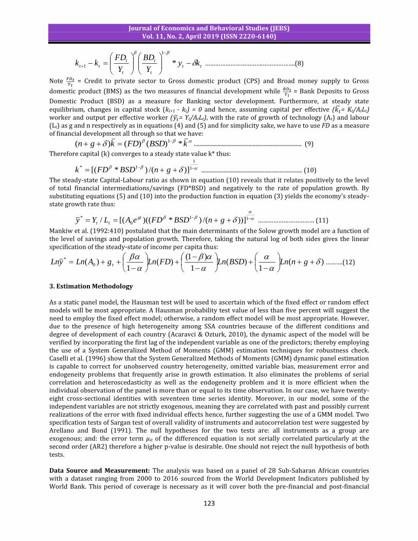
Journal of Economics and Behavioral Studies (JEBS) Vol. 11, No. 2, April 2019 (ISSN 2220-6140)
123
tt
t
t
t
ttt ky
Y
BD
Y
FDkk
*
1
1 …………………………….……………….(8)
Note
= Credit to private sector to Gross domestic product (CPS) and Broad money supply to Gross
domestic product (BMS) as the two measures of financial development while
= Bank Deposits to Gross
Domestic Product (BSD) as a measure for Banking sector development. Furthermore, at steady state equilibrium, changes in capital stock (kt+1 - kt) = 0 and hence, assuming capital per effective (
= Kt/AtLt) worker and output per effective worker ( = Yt/AtLt), with the rate of growth of technology (At) and labour (Lt) as g and n respectively as in equations (4) and (5) and for simplicity sake, we have to use FD as a measure of financial development all through so that we have:
kBSDFDkgn *)()()( 1 ............................................................................. (9)
Therefore capital (k) converges to a steady state value k* thus:
1
1
1* )]/()*[( gnBSDFDk ........................................................................ (10)
The steady-state Capital-Labour ratio as shown in equation (10) reveals that it relates positively to the level of total financial intermediations/savings (FD*BSD) and negatively to the rate of population growth. By substituting equations (5) and (10) into the production function in equation (3) yields the economy’s steady-state growth rate thus:
11
0
* ))]/()*)(([(/ gnBSDFDeALYy gt
tt …………………………… (11)
Mankiw et al. (1992:410) postulated that the main determinants of the Solow growth model are a function of the level of savings and population growth. Therefore, taking the natural log of both sides gives the linear specification of the steady-state of income per capita thus:
)(1
)(1
)1()(
1)( 0
*
gnLnBSDLnFDLngALnyLn t ……….(12)
3. Estimation Methodology As a static panel model, the Hausman test will be used to ascertain which of the fixed effect or random effect models will be most appropriate. A Hausman probability test value of less than five percent will suggest the need to employ the fixed effect model; otherwise, a random effect model will be most appropriate. However, due to the presence of high heterogeneity among SSA countries because of the different conditions and degree of development of each country (Acaravci & Ozturk, 2010), the dynamic aspect of the model will be verified by incorporating the first lag of the independent variable as one of the predictors; thereby employing the use of a System Generalized Method of Moments (GMM) estimation techniques for robustness check. Caselli et al. (1996) show that the System Generalized Methods of Moments (GMM) dynamic panel estimation is capable to correct for unobserved country heterogeneity, omitted variable bias, measurement error and endogeneity problems that frequently arise in growth estimation. It also eliminates the problems of serial correlation and heteroscedasticity as well as the endogeneity problem and it is more efficient when the individual observation of the panel is more than or equal to its time observation. In our case, we have twenty-eight cross-sectional identities with seventeen time series identity. Moreover, in our model, some of the independent variables are not strictly exogenous, meaning they are correlated with past and possibly current realizations of the error with fixed individual effects hence, further suggesting the use of a GMM model. Two specification tests of Sargan test of overall validity of instruments and autocorrelation test were suggested by Arellano and Bond (1991). The null hypotheses for the two tests are: all instruments as a group are exogenous; and: the error term μit of the differenced equation is not serially correlated particularly at the second order (AR2) therefore a higher p-value is desirable. One should not reject the null hypothesis of both tests. Data Source and Measurement: The analysis was based on a panel of 28 Sub-Saharan African countries with a dataset ranging from 2000 to 2016 sourced from the World Development Indicators published by World Bank. This period of coverage is necessary as it will cover both the pre-financial and post-financial

Journal of Economics and Behavioral Studies (JEBS) Vol. 11, No. 2, April 2019 (ISSN 2220-6140)
124
crisis of 2007/2008 and periods when most financial reforms took place among African economies. Moreover, given that Sub-Saharan African economies are the study area due to the underdeveloped state of its financial sector and invariably financial intermediate, twenty-eight of SSA economies were selected based on availability of data and a well-structured credit markets that intermediates for funds. The variables of interest based on the theoretical model are per capita GDP (GDPPP) as the explained variable and the explanatory variables includes ratio of credit provided to private sector to GDP (CPS), broad money supply to GDP (BMS) as measures of financial development, tertiary school enrolment (TSR) to capture effective labour, gross capital formation as a ratio of GDP (GCF) to measure investment, foreign direct investment (FDI) to measure technology level and the level of trade openness (TOP) as the control variables.
Model Specification: The econometric form of model (12) for this study based on the augmented theoretical growth model of Solow (1956) and Mankiw et al. (1992) affirms that an economy continues to grow as long as they maintain a consistent flow in their technology augmenting labour-capital ratio, hence it is adjusted to observe that credit extension and banking sector development promotes growth in the following order. By widening the scope of the initial technology base (A0) to include institutions, endowment and climate among other things which may differ across countries to give the model a robust application provided they can be supported by economic theory, Mankiw et al. (1992:411) specified A0 as:
A0 = λ0 +ε …………………………………………..…………………………… (13)
Where λ0 is a constant and ε represents country’s specific shocks. Therefore in our model, λ0 can specify to include a definition of Gross capital formation to GDP (GCF), effective labour (TSR) and foreign direct investment (FDI) in a Cobb-Douglas function thus: A0 = λ0GCF λ1TSR λ2FDI λ3eε ……………………………………………………... (14)
Taking the log form of equation (14), substituting it into (12) and for uniformity sake, let
1= λ4;
1
)1(= λ5 and
1= λ6 to yield a panel model to be estimated thus:
Note: FD = {CPS, BMS}
ititititititititit TOPBSDBSDFDFDITSRGCFy 7
2
6543210
* .. (15)
Where y* is real per capita income growth rate, λ1, λ2 and λ3 are the shares of gross capital formation as a ratio of GDP (a proxy for investment), tertiary school enrolment (TSR) a measure of effective labour, foreign direct investment (FDI) a measure of technology transfer respectively to growth; while λ4 and λ5 represents the proportions of savings (credit to private sector and broad money supply to GDP), banking sector development (BSD) respectively to growth; and λ7 is the parameter of the control variable trade openness (TOP) to output growth; CPS and BSD are the levels of financial and banking sector development respectively; and n, g and δ are as defined above. Furthermore, in their specification, Mankiw et al. (1992:412) assumes that g and δ are constant across countries; whereas g is primarily the advancement of knowledge, which is country specific. δ the rate of capital depreciation is constant across countries; therefore g and δ are superimposed in the error term (ε) and the constant term (λ0) respectively as represented in model (15).
Model 15 also follows that of Sassi & Goaied (2013) and Vu (2011) by incorporating a quadratic function to account for the long run non-linear relationship between banking sector development and growth. The null hypothesis here is that improved banking sector development, in the long run, will get to a point where it becomes productive and promotes overall growth which will not be rejected if the parameter estimate of banking sector development quadratic term is both positive and statistically significant. The policy implication here is that it is only when this condition is fulfilled that banking sector development can form a transmission channel of financial development to growth in the long run. Given this, we, therefore, go further to specify an interactive model between financial development and banking sector development terms in the next equation to check whether the ability of financial development to impact on growth depends on the level
of improved development in the banking sector and for the sake of uniqueness, we use instead of :
ititititititititit TOPFDBSDBSDFDFDITSRGCFy 76543210
* )( ... (16)

Journal of Economics and Behavioral Studies (JEBS) Vol. 11, No. 2, April 2019 (ISSN 2220-6140)
125
4. Results and Discussion The findings from the estimation results will be presented in this section starting with summary statistics to see the overall behaviour and relationships among the variables. After which a standard growth model as specified in equation 1 above will be estimated to show how financial development and banking sector development individual impacts growth. This is followed by a non-linear growth model to account for the long run effect of banking sector development on growth as this will measure to what extent will increased bank development will get to before it begins to accelerate or hamper growth among Sub-Saharan Africa; and finally, the analysis will estimate the interactive impact of financial development and bank development as a transmission channel to growth. Summary Statistics: The summary statistics show that the analysis made use of nine endogenous and exogenous variables with 476 data series comprising of twenty-eight cross-sectional units and seventeen-time variant identity. The mean, median, standard deviation, minimum, maximum, Skewness and Kurtosis results were presented. Trade openness shows has the highest mean value as well as the largest highest standard deviation. This means that its dispersion from the mean is largest compared to other series in the model. The average growth rate among SSA countries stood at 2.33 percent per annum with a very high financial development indicator at 31.82 percent (M2/GDP) and 22.81 percent (credit to private sector/GDP). With these results, it is expected that with reasonable intermediation efficiency on the side of the bank financial institutions, financial development should trigger substantial growth and welfare among the people for the period under consideration. The statistics show that the average banking sector development stood at an average rate of 24.24 percent, which is still very low to spur growth among SSA countries. This hypothesis will be justified under model (16) estimation results. Finally, on this note, the summary statistics reveal that our series is not normally distributed because the p-values of the Jarque-Bera statistics were all less than 5 percent. Since the probability value of the Hausman test on whether to employ the fixed effect or random effect model is less than 5 percent, thereby suggesting the use of a fixed effect model, the result of the fixed effect estimation of model 15 is presented in table 1 below: The result output as presented in table one is a four-model estimate of equation 15. The first two models is a fixed effect model with two measure of financial development as broad money to GDP (BMS) and credit to private sector to GDP (CPS) respectively whereas the last two models present the system GMM result in the same manner. Table 1: A Fixed Effect and System GMM Estimate of Model 15 Fixed Effect model System GMM Model Dependent Variable GDPPR(1) GDPPR(2) GDPPR (3) GDPPR (4) Constant -0.651 -0.725 -2.598 -1.627 (0.46) (0.52) (2.16)* (1.56) GCF 0.138 0.139 0.231 0.168 (3.94)** (3.97)** (6.40)** (4.37)** TSR -0.030 -0.029 0.010 -0.014 (1.21) (1.19) (0.49) (0.74) FDI 0.037 0.037 -0.061 -0.042 (0.84) (0.82) (1.30) (0.90) BMS -0.013 0.176 (0.22) (2.66)** CPS 0.006 0.058 (0.17) (3.35)** BSD -0.198 -0.217 -0.342 -0.201 (2.15)* (2.93)** (3.96)** (3.51)** BSD^2 0.001 0.001 0.001 0.001 (1.99)* (1.98)* (2.51)* (2.43)* TOP 0.054 0.053 0.007 0.032 (3.51)** (3.48)** (0.60) (2.23)* L. GDPPR NA NA 0.174 0.160 NA NA (3.35)** (3.01)** AR2 NA NA 0.209 0.135
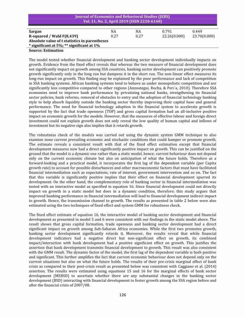
Journal of Economics and Behavioral Studies (JEBS) Vol. 11, No. 2, April 2019 (ISSN 2220-6140)
126
Sargan NA NA 0.791 0.449 R-squared / Wald F(8,439) 0.27 0.27 22.26(0.000) 23.70(0.000) Absolute value of t statistics in parentheses * significant at 5%; ** significant at 1% Source: Estimation The model tested whether financial development and banking sector development individually impacts on growth. Evidence from the fixed effect reveals that whereas the two measure of financial development does not significantly impact on growth among SSA countries, banking sector development can positively promote growth significantly only in the long run but dampens it in the short run. The non-linear effect measures its long-run impact on growth. This finding may be explained by the poor performance and lack of competition in SSA banking systems. African banking systems tend to behave as under monopolistic competition and are significantly less competitive compared to other regions (Anzoategui, Rocha, & Perı´a, 2010). Therefore SSA economies need to improve bank performance by privatizing national banks, strengthening its financial sector policies, bank reforms, removal of obstacles to entry and the adoption of financial technology banking style to help absorb liquidity outside the banking sector thereby improving their capital base and general performance. The need for financial technology adoption in the financial system to accelerate growth is supported by the fact that trade openness (TOP) and gross capital formation had an all-inclusive positive impact on economic growth for the models. However, that the measures of effective labour and foreign direct investment could not explain growth does not only reveal the low quality of human capital and inflows of investment but its negative sign also implies that it retards growth. The robustness check of the models was carried out using the dynamic system GMM technique to also examine none current prevailing economic and stochastic conditions that could hamper or promote growth. The estimate reveals a consistent result with that of the fixed effect estimation except that financial development measures now had a direct significantly positive impact on growth. This can be justified on the ground that the model is a dynamic one rather than a static model, hence; current behaviour does not depend only on the current economic climate but also on anticipation of what the future holds. Therefore as a forward-looking and a practical model, it incorporates the first lag of the dependent variable (per Capita growth rate) to account for possible disturbances and other macroeconomic factors that must have facilitated financial intermediation such as expectations, rate of interest, government intervention and so on. The fact that this variable is significantly positive implies that their effect on financial development spurred its development. On the other hand, the complementary role of banking sector in financial intermediation was tested with an interactive model as specified in equation 16. Since financial development could not directly impact on growth in a static model but does in a dynamic condition, therefore; this study argues that improved banking performance in financial intermediation will lead to financial development indirect impact to growth. Hence, the transmission channel to growth. The results as presented in table 2 below were also estimated using the two techniques of fixed effect and system GMM for robustness check. The fixed effect estimate of equation 16, the interactive model of banking sector development and financial development as presented in model 5 and 6 were consistent with our findings in the static model above. The result shows that gross capital formation, trade openness and banking sector development had a direct significant impact on growth among Sub-Saharan Africa economies. While the first two promotes growth, banking sector development significantly retards it. Moreover, the results reveal that while financial development indicators had a negative direct but non-significant effect on growth, its combined impact/interaction with bank development had a positive significant effect on growth. This justifies the assertion that bank development transmits financial development to growth. This result was also consistent with the GMM result. The dynamic factor of the model, the first lag of the dependent variable is both positive and significant. This further amplifies the fact that current economic behaviour does not depend only on the current situations but also on what the future holds. The results of their pre-crisis marginal effect of bank crisis as compared to their post-crisis result as presented below was consistent with Caggiano et al. (2014) assertion. The results were estimated using equations 15 and 16 for the marginal effects of bank sector development (MEBSD) to ascertain whether there are any substantial changes in the banking sector development (BSD) interacting with financial development to foster growth among the SSA region before and after the financial crisis of 2007/08.
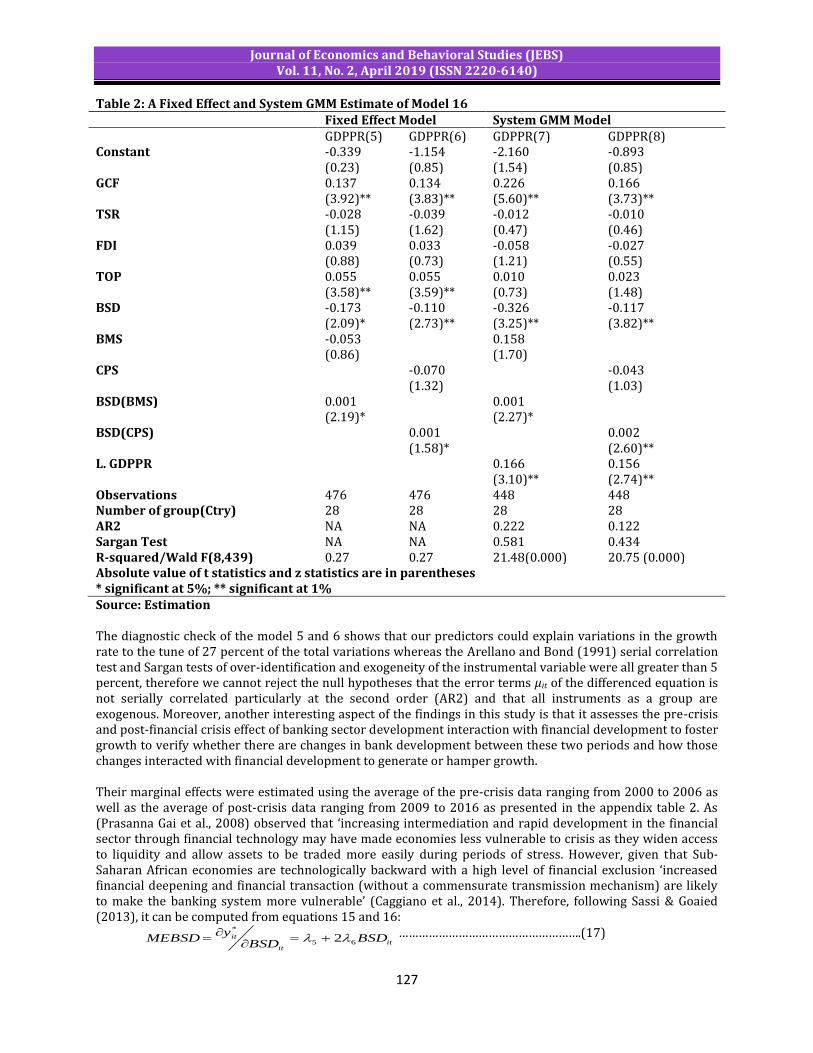
Journal of Economics and Behavioral Studies (JEBS) Vol. 11, No. 2, April 2019 (ISSN 2220-6140)
127
Table 2: A Fixed Effect and System GMM Estimate of Model 16 Fixed Effect Model System GMM Model GDPPR(5) GDPPR(6) GDPPR(7) GDPPR(8) Constant -0.339 -1.154 -2.160 -0.893 (0.23) (0.85) (1.54) (0.85) GCF 0.137 0.134 0.226 0.166 (3.92)** (3.83)** (5.60)** (3.73)** TSR -0.028 -0.039 -0.012 -0.010 (1.15) (1.62) (0.47) (0.46) FDI 0.039 0.033 -0.058 -0.027 (0.88) (0.73) (1.21) (0.55) TOP 0.055 0.055 0.010 0.023 (3.58)** (3.59)** (0.73) (1.48) BSD -0.173 -0.110 -0.326 -0.117 (2.09)* (2.73)** (3.25)** (3.82)** BMS -0.053 0.158 (0.86) (1.70) CPS -0.070 -0.043 (1.32) (1.03) BSD(BMS) 0.001 0.001 (2.19)* (2.27)* BSD(CPS) 0.001 0.002 (1.58)* (2.60)** L. GDPPR 0.166 0.156 (3.10)** (2.74)** Observations 476 476 448 448 Number of group(Ctry) 28 28 28 28 AR2 NA NA 0.222 0.122 Sargan Test NA NA 0.581 0.434 R-squared/Wald F(8,439) 0.27 0.27 21.48(0.000) 20.75 (0.000) Absolute value of t statistics and z statistics are in parentheses * significant at 5%; ** significant at 1% Source: Estimation The diagnostic check of the model 5 and 6 shows that our predictors could explain variations in the growth rate to the tune of 27 percent of the total variations whereas the Arellano and Bond (1991) serial correlation test and Sargan tests of over-identification and exogeneity of the instrumental variable were all greater than 5 percent, therefore we cannot reject the null hypotheses that the error terms μit of the differenced equation is not serially correlated particularly at the second order (AR2) and that all instruments as a group are exogenous. Moreover, another interesting aspect of the findings in this study is that it assesses the pre-crisis and post-financial crisis effect of banking sector development interaction with financial development to foster growth to verify whether there are changes in bank development between these two periods and how those changes interacted with financial development to generate or hamper growth. Their marginal effects were estimated using the average of the pre-crisis data ranging from 2000 to 2006 as well as the average of post-crisis data ranging from 2009 to 2016 as presented in the appendix table 2. As (Prasanna Gai et al., 2008) observed that ‘increasing intermediation and rapid development in the financial sector through financial technology may have made economies less vulnerable to crisis as they widen access to liquidity and allow assets to be traded more easily during periods of stress. However, given that Sub-Saharan African economies are technologically backward with a high level of financial exclusion ‘increased financial deepening and financial transaction (without a commensurate transmission mechanism) are likely to make the banking system more vulnerable’ (Caggiano et al., 2014). Therefore, following Sassi & Goaied (2013), it can be computed from equations 15 and 16:
itit
it BSDBSD
yMEBSD 65
*
2
……………………………………………….(17)
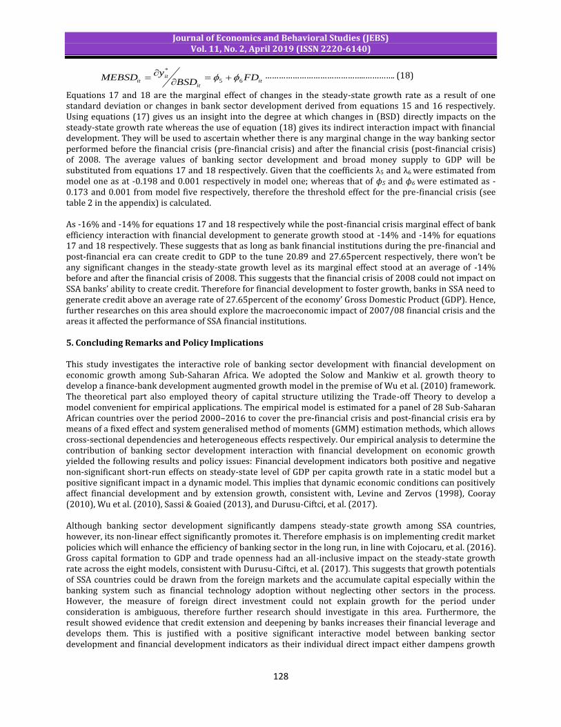
Journal of Economics and Behavioral Studies (JEBS) Vol. 11, No. 2, April 2019 (ISSN 2220-6140)
128
it
it
itit FD
BSDy
MEBSD 65
*
……………………………………..…………. (18)
Equations 17 and 18 are the marginal effect of changes in the steady-state growth rate as a result of one standard deviation or changes in bank sector development derived from equations 15 and 16 respectively. Using equations (17) gives us an insight into the degree at which changes in (BSD) directly impacts on the steady-state growth rate whereas the use of equation (18) gives its indirect interaction impact with financial development. They will be used to ascertain whether there is any marginal change in the way banking sector performed before the financial crisis (pre-financial crisis) and after the financial crisis (post-financial crisis) of 2008. The average values of banking sector development and broad money supply to GDP will be substituted from equations 17 and 18 respectively. Given that the coefficients λ5 and λ6 were estimated from model one as at -0.198 and 0.001 respectively in model one; whereas that of ϕ5 and ϕ6 were estimated as -0.173 and 0.001 from model five respectively, therefore the threshold effect for the pre-financial crisis (see table 2 in the appendix) is calculated. As -16% and -14% for equations 17 and 18 respectively while the post-financial crisis marginal effect of bank efficiency interaction with financial development to generate growth stood at -14% and -14% for equations 17 and 18 respectively. These suggests that as long as bank financial institutions during the pre-financial and post-financial era can create credit to GDP to the tune 20.89 and 27.65percent respectively, there won’t be any significant changes in the steady-state growth level as its marginal effect stood at an average of -14% before and after the financial crisis of 2008. This suggests that the financial crisis of 2008 could not impact on SSA banks’ ability to create credit. Therefore for financial development to foster growth, banks in SSA need to generate credit above an average rate of 27.65percent of the economy’ Gross Domestic Product (GDP). Hence, further researches on this area should explore the macroeconomic impact of 2007/08 financial crisis and the areas it affected the performance of SSA financial institutions. 5. Concluding Remarks and Policy Implications This study investigates the interactive role of banking sector development with financial development on economic growth among Sub-Saharan Africa. We adopted the Solow and Mankiw et al. growth theory to develop a finance-bank development augmented growth model in the premise of Wu et al. (2010) framework. The theoretical part also employed theory of capital structure utilizing the Trade-off Theory to develop a model convenient for empirical applications. The empirical model is estimated for a panel of 28 Sub-Saharan African countries over the period 2000–2016 to cover the pre-financial crisis and post-financial crisis era by means of a fixed effect and system generalised method of moments (GMM) estimation methods, which allows cross-sectional dependencies and heterogeneous effects respectively. Our empirical analysis to determine the contribution of banking sector development interaction with financial development on economic growth yielded the following results and policy issues: Financial development indicators both positive and negative non-significant short-run effects on steady-state level of GDP per capita growth rate in a static model but a positive significant impact in a dynamic model. This implies that dynamic economic conditions can positively affect financial development and by extension growth, consistent with, Levine and Zervos (1998), Cooray (2010), Wu et al. (2010), Sassi & Goaied (2013), and Durusu-Ciftci, et al. (2017). Although banking sector development significantly dampens steady-state growth among SSA countries, however, its non-linear effect significantly promotes it. Therefore emphasis is on implementing credit market policies which will enhance the efficiency of banking sector in the long run, in line with Cojocaru, et al. (2016). Gross capital formation to GDP and trade openness had an all-inclusive impact on the steady-state growth rate across the eight models, consistent with Durusu-Ciftci, et al. (2017). This suggests that growth potentials of SSA countries could be drawn from the foreign markets and the accumulate capital especially within the banking system such as financial technology adoption without neglecting other sectors in the process. However, the measure of foreign direct investment could not explain growth for the period under consideration is ambiguous, therefore further research should investigate in this area. Furthermore, the result showed evidence that credit extension and deepening by banks increases their financial leverage and develops them. This is justified with a positive significant interactive model between banking sector development and financial development indicators as their individual direct impact either dampens growth

Journal of Economics and Behavioral Studies (JEBS) Vol. 11, No. 2, April 2019 (ISSN 2220-6140)
129
or could not significantly explain the growth. Therefore the need to promote financial institutions’ efficiency through deregulation, bank reforms and monetary policy measures cannot be overemphasized. This assertion is strengthened by the significant impact of the policy parameter, the lag of income Per-Capita growth rate in a dynamic economic condition. Finally, the marginal effects of bank development on steady-state growth reveal that there was no significant difference in the ability of banks to mobilize savings for investment purposes for the two time zones, pre-financial crisis 2000-2007 and the post-financial period 2009-2016. This implies that banking sector in SSA is relatively consistent in generating growth through financial intermediation, thereby promoting macroeconomic stability and investors’ confidence. However, the negative effect of bank sector’s marginal effect on growth is an indication of the underdeveloped state of the sector. Therefore the need for institutional and legal improvements that strengthen creditor and investor rights and contract enforcement as well as increasing financial inclusion through financial technology adoption should be enforced to promote financial markets’ stability and overall economic performance. References Acaravci, A. & Ozturk, I. (2010). Electricity consumption-growth nexus: Evidence from panel data for
transition countries. Energy Economics, 32(3), 604-608. Anzoategui, D., Rocha, R. & Perı´a, S. M. (2010). Bank competition in the Middle East and Northern Africa
Region. Review of Middle East Economics and Finance, 6(2), 26–48. Anzoategui, D., Martinez, P. M. S. & Rocha, R. R. (2010). Bank Competition in the Middle East and Northern
Africa Region, Review of Middle East Economics and Finance, 6(2), 26–48. Arellano, M. & Bond, S. (1991). Some tests of specification for panel data: Monte Carlo evidence and an
application to employment equations. The review of economic studies, 58(2), 277-297. Arestis, P., Chortareas, G. & Desli, E. (2006). Financial development and productive efficiency in OECD
countries: an exploratory analysis. The Manchester School, 74(4), 417-440. Caggiano, G., Calice, P. & Leonida, L. (2014). Early warning systems and systemic banking crises in low-
income countries: A multinomial logit approach. Journal of Banking & Finance, 47, 258-269. Caselli, F., Esquivel G. & Lefort, F. (1996). Reopening the Convergence Debate: A New Look at Cross-Country
Growth Empirics. Journal of Economic Growth, 1(3), 363-389. Cojocaru, L., Falaris, E. M., Hoffman, S. D. & Miller, J. B. (2016). Financial system development and economic
growth in transition economies: New empirical evidence from the CEE and CIS countries. Emerging Markets Finance and Trade, 52(1), 223-236.
Cooray, A. (2010). Do stock markets lead to economic growth? Journal of Policy Modelling, 32(4), 448-460. Durusu-Ciftci, D., Ispir, M. S. & Yetkiner, H. (2017). Financial development and economic growth: Some theory
and more evidence. Journal of Policy Modelling, 39(2), 290-306. Ferreira, C. (2013). Bank performance and economic growth: evidence from Granger panel causality
estimations. Gai, P., Kapadia, S., Millard, S. & Perez, A. (2008). Financial innovation, macroeconomic stability and systemic
crises. The Economic Journal, 118(527), 401-426. Gurley, J. G. & Shaw, E. S. (1960). Money in a theory of finance. Washington, DC: Brookings Institution Gregorio, J. & Guidotti, P. E. (1992). Financial development and economic growth. International Monetary Fund
working paper 92/101. Hasan, I., Koetter, M., Lensink, R. & Meesters, A. (2008). Bank efficiency, financial depth, and economic
growth. Iheanacho, E. (2016). The impact of financial development on economic growth in Nigeria: An ARDL analysis. Economies, 4(4), 26.
Hondroyiannis, G., Lolos, S. & Papapetrou, E. (2005). Financial markets and economic growth in Greece, 1986–1999. Journal of International Financial Markets, Institutions and Money, 15(2), 173-188.
Huang, H. C. & Lin, S. C. (2009). Non‐linear finance-growth nexus: A threshold with instrumental variable approach 1. Economics of Transition, 17(3), 439-466.
Killick, T. (1991). Financial management and economic development: some issues. South African Journal of Economics, 59(3), 167-180.
Kpodar, K. & Andrianaivo, M. (2011). ICT, financial inclusion, and growth evidence from African countries (No. 11-73). International Monetary Fund.

Journal of Economics and Behavioral Studies (JEBS) Vol. 11, No. 2, April 2019 (ISSN 2220-6140)
130
Levine, R. & Zervos, S. (1998). Stock markets, banks and economic growth. The American Economic Review, 88, 537–558.
Levine, R., Loayza, N. & Beck, T. (2000). Financial intermediation and growth: Causality and causes. Journal of Monetary Economics, 46(1), 31-77.
Levine, R. (2004). Finance and growth: theory and evidence: NBER Working Paper Series n. 10766. Luintel, K. B. & Khan, M. (1999). A quantitative reassessment of the finance-growth nexus: evidence from a
multivariate VAR. Journal of development economics, 60(2), 381-405. Mankiw, N. G., Romer, D. & Weil, D. N. (1992). A contribution to the empirics of economic growth. The
quarterly journal of economics, 107(2), 407-437. McKinnon, R. I. (1973). Money and Capital in Economic Development. Washington, DC: Brookings Institution,
1973; Shaw, E. Financial Deepening in Economic Development. Nzotta, S. M. & Okereke, E. J. (2009). Financial deepening and economic development of Nigeria: An Empirical
Investigation. Pagano, M. (1993). Financial markets and growth: an overview. European economic review, 37(2-3), 613-622. Rioja, F. & Valev, N. (2004). Finance and the sources of growth at various stages of economic development.
Economic Inquiry, 42(1), 127-140. Sassi, S. & Goaied, M. (2013). Financial development, ICT diffusion and economic growth: Lessons from MENA
region. Telecommunications Policy, 37(4-5), 252-261. Shamim, F. (2007). The ICT environment, financial sector and economic growth: a cross-country analysis.
Journal of Economic Studies, 34(4), 352–370. Solow, R. M. (1956). A contribution to the theory of economic growth. The quarterly journal of economics,
70(1), 65-94. Torruam, J. T., Chiawa, M. A. & Abur, C. C. (2013). Financial deepening and economic growth in Nigeria: an
application of co-integration and causality analysis. In 3rd International Conference on Intelligent Computational System (ICIC’2013). April (pp. 29-30).
Vu, K. M. (2011). ICT as a source of economic growth in the information age: Empirical evidence from the 1996–2005 period. Telecommunications Policy, 35(4), 357-372.
World Bank. (1982). World Development Report 1989. New York: Oxford University Press for the World Bank.
World Bank. (2013). Financing for Development Report post-2015, October, 2013. Wu, J. L., Hou, H. & Cheng, S. Y. (2010). The dynamic impacts of financial institutions on economic growth:
Evidence from the European Union. Journal of Macroeconomics, 32(3), 879-891.
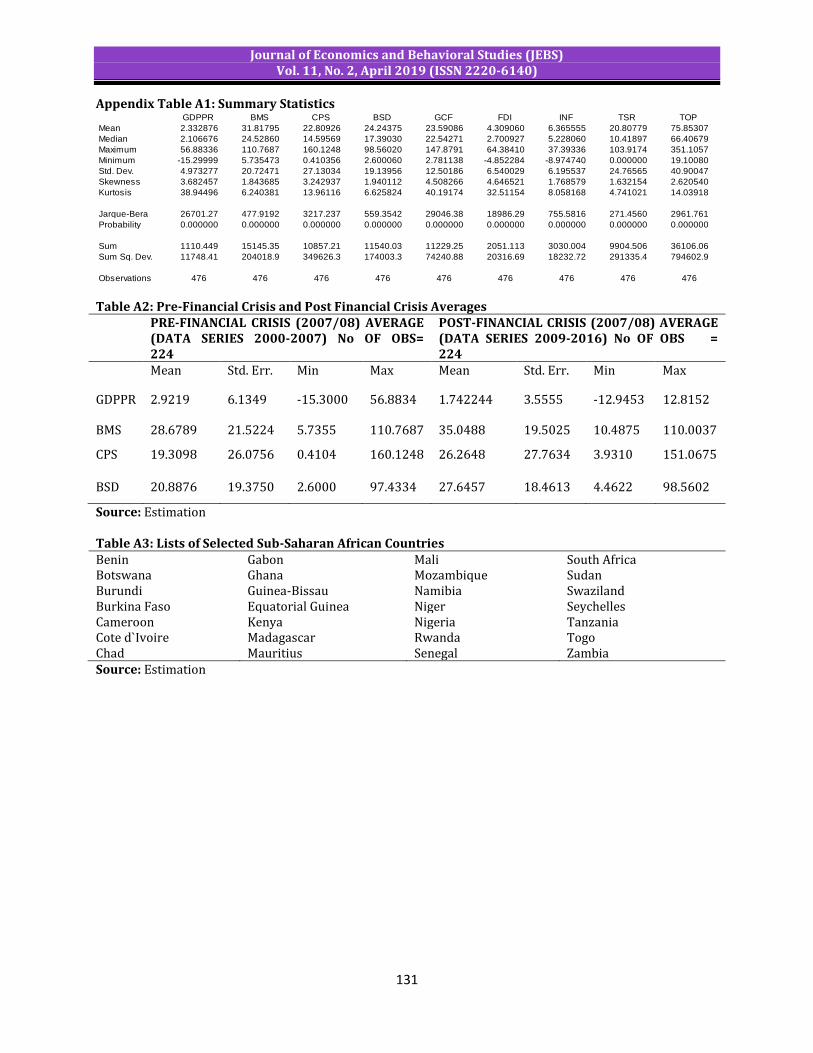
Journal of Economics and Behavioral Studies (JEBS) Vol. 11, No. 2, April 2019 (ISSN 2220-6140)
131
Appendix Table A1: Summary Statistics
Table A2: Pre-Financial Crisis and Post Financial Crisis Averages PRE-FINANCIAL CRISIS (2007/08) AVERAGE
(DATA SERIES 2000-2007) No OF OBS= 224
POST-FINANCIAL CRISIS (2007/08) AVERAGE (DATA SERIES 2009-2016) No OF OBS = 224
Mean Std. Err. Min Max Mean Std. Err. Min Max
GDPPR 2.9219 6.1349 -15.3000 56.8834 1.742244 3.5555 -12.9453 12.8152
BMS 28.6789 21.5224 5.7355 110.7687 35.0488 19.5025 10.4875 110.0037
CPS 19.3098 26.0756 0.4104 160.1248 26.2648 27.7634 3.9310 151.0675
BSD 20.8876 19.3750 2.6000 97.4334 27.6457 18.4613 4.4622 98.5602
Source: Estimation Table A3: Lists of Selected Sub-Saharan African Countries Benin Gabon Mali South Africa Botswana Ghana Mozambique Sudan Burundi Guinea-Bissau Namibia Swaziland Burkina Faso Equatorial Guinea Niger Seychelles Cameroon Kenya Nigeria Tanzania Cote d`Ivoire Madagascar Rwanda Togo Chad Mauritius Senegal Zambia Source: Estimation
GDPPR BMS CPS BSD GCF FDI INF TSR TOP
Mean 2.332876 31.81795 22.80926 24.24375 23.59086 4.309060 6.365555 20.80779 75.85307
Median 2.106676 24.52860 14.59569 17.39030 22.54271 2.700927 5.228060 10.41897 66.40679
Maximum 56.88336 110.7687 160.1248 98.56020 147.8791 64.38410 37.39336 103.9174 351.1057
Minimum -15.29999 5.735473 0.410356 2.600060 2.781138 -4.852284 -8.974740 0.000000 19.10080
Std. Dev. 4.973277 20.72471 27.13034 19.13956 12.50186 6.540029 6.195537 24.76565 40.90047
Skewness 3.682457 1.843685 3.242937 1.940112 4.508266 4.646521 1.768579 1.632154 2.620540
Kurtosis 38.94496 6.240381 13.96116 6.625824 40.19174 32.51154 8.058168 4.741021 14.03918
Jarque-Bera 26701.27 477.9192 3217.237 559.3542 29046.38 18986.29 755.5816 271.4560 2961.761
Probability 0.000000 0.000000 0.000000 0.000000 0.000000 0.000000 0.000000 0.000000 0.000000
Sum 1110.449 15145.35 10857.21 11540.03 11229.25 2051.113 3030.004 9904.506 36106.06
Sum Sq. Dev. 11748.41 204018.9 349626.3 174003.3 74240.88 20316.69 18232.72 291335.4 794602.9
Observations 476 476 476 476 476 476 476 476 476

Journal of Economics and Behavioral Studies (JEBS) Vol. 11, No. 2, April 2019 (ISSN 2220-6140)
132
Dynamics of Ethnic Politics in Nigeria: An Impediment to its Political System
Toyin Cotties Adetiba Department of Politics and International Studies, University of Zululand, KwaDlangezwa, South Africa
[email protected] Abstract: Without any form of prejudice, it is a fact that Nigeria is a multi-ethnic state with differences in its socio-political and economic development all of which have resulted in conflicts and counter conflicts. Ethnic politics in Nigeria’s political system have come to be a tragic and constant in Nigeria’s political system; where one must belong to the mainstream of ethnic politics for political relevance. It depicts attachments to the sub-national ethnic groups which threaten to undermine national integration and therefore divide the nation. Significantly, ethnicity in Nigeria was orchestrated by a long period of colonialism, a period which witnessed the ascendancy of the three major ethnic groups in Nigeria to the socio-political domination of other ethnic groups. It was a period when the three major ethnic groups were used by the colonialist as a pedestal for the distribution of socio-political and economic goods. Using a mixed method, this work argues that Nigeria’s political problem hinges on the negative consequences of ethnic politics. The paper concludes that if Nigeria’s political system must progress, it must be anchored on the need for the review of the constitutional and political structure of Nigeria to restore healthy political competition as opposed to the existing outdated political mechanism imposed on Nigeria by the military under the 1999 Constitution of the Federal Republic of Nigeria. Keywords: Ethnic politics, Development, Globalization, Nationalism, Ethnic loyalty.
1. Introduction If you are born in Nigeria, grow up and trained to become an engineer, lawyer, doctor or a teacher and probably die rich; you remain a Nigerian. But within the context of ethnicity; as long as you remain a Nigerian your political affiliation notwithstanding, your ethnic group is fixed. To Chandra (2012) everyone belongs to one ethnic group, the membership of each group remains for a long period of time, and as it is passed down from generation to generation, along the line there may be war, economic crisis but the fact is ethnic groups does not change. Without the consent and consensus of different tribes/ethnic groups which were over 300, the Nigeria federation was constituted by the British colonialist in the amalgamation of 1914. This action was reinforced by Onwe (2019) that on the formation of Nigeria on January 1, 1914, all the ethnic nationalities were conquered, subdued and placed as the subjects of the British Monarch. This forced/artificial marriage of ethnic groups which emerged upon the British imperial expansion no doubt has significant consequences for political development in Nigeria (Brown, 2013). This anomaly impelled the political leaders to start agitating for de-amalgamation of Nigeria in a bid to forestall the future danger which the forced merger of hitherto independent ethnics groups portended. Significantly, this fundamental error has deepened in contemporary Nigeria, hence the conspicuous differences in Nigeria’s ethnic configuration stretching from language to population, geographical landscape, level of education which the colonialist never considered before the artificial creation of Nigeria. To this end, late Ahmadu Bello in 1944 described the amalgamation of Nigeria as the mistake of 1914 which if allowed to remains will ultimately lead to unstoppable bloodshed and failed country. Lending his voice to Ahmadu Bello’s observation, late Obafemi Awolowo described Nigeria as a mere geographical expression (Brown, 2013) that is not qualified to be called a country not alone a nation and if the amalgamation could not be reversed, then Nigeria should be restructured as strictly a federal state to give room for every ethnic group to enjoy freedom from being dominated by any one single tribe. Contrary to the expected unity, the politics of administration in Nigeria has been offensively punctuated by very disturbing ethnic politics. Brown (2013:172) expound that in Nigeria’s political system, the reconfiguration, formation of political parties, distribution of human and material resources and even crises (coups, civil war, and religious impasse) are hinged on ethno-religious politics. Without any form of prejudice, it is a fact that Nigeria is a multi-ethnic state with differences in its socio-political and economic development all of which have resulted into conflicts and counter conflicts. Notwithstanding the era of globalisation, the level of ethnicity in Nigeria has unabatedly
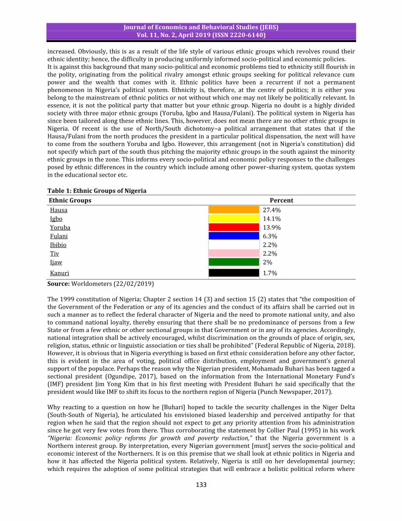
Journal of Economics and Behavioral Studies (JEBS) Vol. 11, No. 2, April 2019 (ISSN 2220-6140)
133
increased. Obviously, this is as a result of the life style of various ethnic groups which revolves round their ethnic identity; hence, the difficulty in producing uniformly informed socio-political and economic policies. It is against this background that many socio-political and economic problems tied to ethnicity still flourish in the polity, originating from the political rivalry amongst ethnic groups seeking for political relevance cum power and the wealth that comes with it. Ethnic politics have been a recurrent if not a permanent phenomenon in Nigeria’s political system. Ethnicity is, therefore, at the centre of politics; it is either you belong to the mainstream of ethnic politics or not without which one may not likely be politically relevant. In essence, it is not the political party that matter but your ethnic group. Nigeria no doubt is a highly divided society with three major ethnic groups (Yoruba, Igbo and Hausa/Fulani). The political system in Nigeria has since been tailored along these ethnic lines. This, however, does not mean there are no other ethnic groups in Nigeria. Of recent is the use of North/South dichotomy–a political arrangement that states that if the Hausa/Fulani from the north produces the president in a particular political dispensation, the next will have to come from the southern Yoruba and Igbo. However, this arrangement (not in Nigeria’s constitution) did not specify which part of the south thus pitching the majority ethnic groups in the south against the minority ethnic groups in the zone. This informs every socio-political and economic policy responses to the challenges posed by ethnic differences in the country which include among other power-sharing system, quotas system in the educational sector etc.
Table 1: Ethnic Groups of Nigeria
Ethnic Groups
Percent
Hausa 27.4%
Igbo 14.1%
Yoruba 13.9%
Fulani 6.3%
Ibibio 2.2%
Tiv 2.2%
Ijaw 2%
Kanuri 1.7%
Source: Worldometers (22/02/2019) The 1999 constitution of Nigeria; Chapter 2 section 14 (3) and section 15 (2) states that “the composition of the Government of the Federation or any of its agencies and the conduct of its affairs shall be carried out in such a manner as to reflect the federal character of Nigeria and the need to promote national unity, and also to command national loyalty, thereby ensuring that there shall be no predominance of persons from a few State or from a few ethnic or other sectional groups in that Government or in any of its agencies. Accordingly, national integration shall be actively encouraged, whilst discrimination on the grounds of place of origin, sex, religion, status, ethnic or linguistic association or ties shall be prohibited” (Federal Republic of Nigeria, 2018). However, it is obvious that in Nigeria everything is based on first ethnic consideration before any other factor, this is evident in the area of voting, political office distribution, employment and government’s general support of the populace. Perhaps the reason why the Nigerian president, Mohamadu Buhari has been tagged a sectional president (Ogundipe, 2017), based on the information from the International Monetary Fund’s (IMF) president Jim Yong Kim that in his first meeting with President Buhari he said specifically that the president would like IMF to shift its focus to the northern region of Nigeria (Punch Newspaper, 2017). Why reacting to a question on how he [Buhari] hoped to tackle the security challenges in the Niger Delta (South-South of Nigeria), he articulated his envisioned biased leadership and perceived antipathy for that region when he said that the region should not expect to get any priority attention from his administration since he got very few votes from there. Thus corroborating the statement by Collier Paul (1995) in his work “Nigeria: Economic policy reforms for growth and poverty reduction,” that the Nigeria government is a Northern interest group. By interpretation, every Nigerian government [must] serves the socio-political and economic interest of the Northerners. It is on this premise that we shall look at ethnic politics in Nigeria and how it has affected the Nigeria political system. Relatively, Nigeria is still on her developmental journey; which requires the adoption of some political strategies that will embrace a holistic political reform where

Journal of Economics and Behavioral Studies (JEBS) Vol. 11, No. 2, April 2019 (ISSN 2220-6140)
134
every ethnic group would be able trust one another in order to achieve its developmental goals. This work uses the indices of ethnic schism based on models of ethnic politics to explain the level of ethnic politics in Nigeria. This paper argues that Nigeria’s political problem hinges on the negative consequences of ethnic politics in the country. It argues that ethnic politics is significant in explaining the prevalence of decay in Nigeria’s political system. 2. Methods Ideally, there are research methods that are specifically meant for an empirical phenomenon of this nature. Research method is commonly classified into qualitative and quantitative methods; this refers to dissimilarities in the nature of knowledge and the purpose for which research is being conducted. This work, however, uses the mixed method. According to Blaikie (2000); Scandura and Williams (2000) this method involves the use of multiple approaches and measures of an empirical phenomenon in order to overcome the challenges of bias and validity. From an ethical point of view, mixed method arose in other to confirm and endorse the rationality of research processes while using multiple sources (Yin, 2003). By implication, this method of approach is opened to utilizing multiple data sources, multiple informants, and multiple methods. Within this premise, this study combines the use of interactive (multiple informants) as well as context analysis to source for information. The first source of information came from Nigerian colleagues on a professional basis here at the University of Zululand. The second is the individuals who had been involved in Nigeria politics and the third is the work of scholars on ethnic politics. Understandably, this method affords the author to establish facts from the experiences of individual and their view, on ethnic politics in Nigeria. Theoretical Explanation: According to Chandra (2012) researches on the effect of ethnicity on socio-political and economic outcomes is driven by the assumption held by the primordialist that ethnic identities are fixed. Identity, to Rothbart and Cherubin, (2009) relies on a common set of narratives, symbols, and a shared sense of group differences. Olayode (2016) defined identity as a combination of socio-cultural characteristics which individuals share, or are presumed to share, with others on the basis of which one group may be distinguished from others. To Alubo (2009) identity is a group concept based on traits peculiar to individual members of a group which provide responses to the question, “Who am I?” This phenomenon has a combination of other layers of inter and intra ethnic relationship which could be gender and class all of which refer to the same person either in self-definition or as defined by others; thus paving the way for ethnic identity that has played a pivotal role in Nigeria’s political destiny. There are two opposing theories (primordialism and constructivism) that can be explored to explain the phenomenon. To the primordialist, ethnicity is explained as a social association, which is inherent while the constructivist sees ethnicity as an identity, which is socially and culturally constructed (Olayode, 2016). As human beings, the primordialist believes that ethnic identity is inborn with natural connections and to some people which has produced natural divisions with others whether based on race, religion, language or location (Geertz, 1973). Mamdani argues that if ethnicity is considered to be primordial, it means ethnic politics [in Nigeria] would be inherent, thus leading to a Hobbesian war where every ethnic group naturally compete and fight for their own political interests (Mamdani, 2002). Ethnicity in this work is viewed as a social construct, thus implying a differentiation between a particular group and the other perceived as being different. Berman (1998:310) sees the understanding of ethnicity as a socially constructed phenomenon, the outcome of the continuous and generally conflict-ridden interaction of socio-political, economic, religious and cultural forces both external and internal to developing ethnic communities. As Olayode (2016) puts it, ethnicity does not by itself explain ethnic politics, but the exploitation of ethnicity by political actors for their political and economic interests drives ethnic politics. Therefore, from the constructivist approach, ethnicity is not a fixed condition, but a [socio-political] process that is subject to continuous change. That Africa is not culturally, a homogeneous society with multiples of conflicting versions of culture and interests is a function of its susceptibility to been reconstructed along ethnic lines (Peel, 1989). Berman (1998:305) contends that post-colonial African ethnicity is a social construct as a reaction to the socio-political, economic and cultural and political forces of colonialism. He further argues that African ethnic invention emerged as a result of internal struggles over differential access to the resources of modernity and economic accumulation. Hence Berman’s conclusion that those ethnicities were, in particular, the creations of

Journal of Economics and Behavioral Studies (JEBS) Vol. 11, No. 2, April 2019 (ISSN 2220-6140)
135
elites seeking the basis for a conservative modernization. In essence, ethnicity is the product of an unending historical progression, grounded in the past and permanently in creation. By implication, ethnic identity cannot be conjured out of thin air; it must be built on real socio-cultural experience (Gellner, 1983). Therefore, before ethnicity can be utilised as the basis for political mobilization and action, it must be a work of intellectual construction, an invention of a common history, language and culture. Consequently, ethnicity has become an issue in [Nigerian] African societies because previous identities and solidarities were being called into question, as ethnic identity provided a stable core of belonging and continuity with the pasts in a world of snowballing instability (Erikson, 1991). This translates to mean that ethnic mobilization explains and reshapes the role of ethnicity in Nigerian politics (Akpan, 2007). Ethnicity as a mark of political identity in Nigeria predictably occupies a great space within the Nigerian political sphere; it is more or less the easiest and naturally the easiest way for the political class to mobilize people around basic human needs such as security, food, shelter, economic well-being etc. (Kelman, 2007). Hence the supposition that, ethnicity has become a sort of universal shorthand that marks a host of much more complex issues of identity and difference (Broch-Due, 2005). Based on the possibility of change in ethnic identity, Chandra (2012) believes that ethnic diversity can sometimes serve as a pedestal for strengthening rather than threatening democracy, preventing rather than producing violence, and inhibiting rather than accelerating state collapse or secession thus justifying the constructivists’ assertion that ethnic identity does change as time goes on. This is corroborated by Olayode (2016:244) that ethnic identity as a social construct and a dynamic process is, in reality, a fluctuant ingredient subject to alliances, mobilizations and manipulations. Through this, society is intensely differentiated and splintered along political affiliations, which in turn has debilitating consequences for socio-political and economic development. 3. Conceptual Discussion (Review of Literature) Ethnicity and ethnic politics in African society (IES) have become so imperative thus making the question of ethnicity to be one of the most topical issues of study by social scientist owing to the fact that it is debatably, one of the factors responsible for the continent’s socio-economic and political difficulties. Scholars such as Easterly and Levine (1997), Posner (2004), Buhaug (2006), Easterly (2001), Barr and Oduro (2002) Milanovic (2003), Miguel and Gugerty (2005) and Kimenyi (2006) has argued that Africa’s ethnic diversity remained an impeccable factor responsible for its low socio-economic growth, political instability and conflict, high inequality amongst the populace and low or lack of service delivery – public goods. Berman (1998); Blanton, Mason, and Athow (2001) opines that the colonial period had a profound and debilitating effect on ethnicity in Africa, for a variety of reasons. It’s been suggested that colonialists directly promoted ethnic diversity through divide and rule (cost-saving) tactics thus promoting ethnic differences (Laitin, 1994). During the colonial era, ethnicity was rooted in the alliances of the indigenous uneducated leaders, integrating a well defined ethnically governmental system where the local population was involved in the bureaucratic authoritarianism by incorporating them into the pre-colonial patron-client relations (Berman, 1998). Hence the assumption that the constructivist modern processes of economic and political development have overwhelmingly moulded ethnic identities in Africa. In the post-colonial period most African states have done very little to promote nation-building and ethnic harmonisation, but rather focusing on superficial policies alongside the promotion of deep ethnic divisions that contributed to pervasive patron-client relations and by extension to political and economic instability (Green, 2011). The controversies around ethnicity seem to have been heated up by the high visibility of mobilized and politicized ethnic groups in most multi-ethnic states. Therefore, the extent to which ethnic nationalities are able to effectively manage the interplay of ethnic difference determines to what extent a multi-ethnic nation develops without a crisis (Adetiba, 2013). Snodgrass (1995) argues that multi-ethnic developing states are often faced with the challenges of achieving sustainable economic development coupled with the task of managing often volatile inter-ethnic relations. He further argued that many of such states are besieged by lingering underdevelopment and political conflicts. They are under-represented among the fastest growing economies of the world, and are over-represented among low income or slow-growing economies, apart from featuring prominently on the list of countries that have suffered from civil war and [on going] insurgencies. This was the case in Nigeria. Significantly, ethnicity

Journal of Economics and Behavioral Studies (JEBS) Vol. 11, No. 2, April 2019 (ISSN 2220-6140)
136
in Nigeria was orchestrated by a long period of colonialism, a period which witnessed the ascendancy of the three major ethnic groups (Yoruba, Igbo and Hausa/Fulani) to the socio-political domination of other ethnic groups. It was a period when these three major ethnic groups were used by the colonialist as a pedestal for the distribution of socio-political and economic goods. This has continued to impact negatively on the forces of national integration and cohesion in ethnically divided Nigeria to date. This legacy of pervasive patron-client relations and a complex ethnic dialectic of assimilation, fragmentation and competition have persisted in post-colonial Nigerian society, a phenomenon that has since remained fundamental. If not central in Nigeria’s political governance, thus accounting for the personalistic, materialistic and opportunistic character of Nigeria’s politics; undermining its socio-economic and political transformation (Berman 1998). Hence the favor enjoys by a particular ethnic group when political leaders from co-ethnic group control political power when deciding with whom to ally and to whom to distribute public goods (Wimmer, et al., 2009). Ethnicity has therefore provided individuals and groups with their most important political resource in the competition for the scarce goods of modernity, as well as for access to local resources. What the above portends to mean is that in a plural society like Nigeria political activities tend to be organized along ethnic lines no matter how “national” the political parties in the country seems to be. Hence, the assumption of the diversity-breeds-conflict school that demographic index of heterogeneity is likely to overlook how ethnicity relates to the state (Wimmer, et al., 2009: 317) while endangering national integration as well as inclusive development, where national integration is conceived as a process that unites people with different culture and social background into a national unit. In essence, a recognised national identity is significant to overcoming the dynamics of problems created by ethnic politics. The main thrust of national integration which in the long run leads to development is to create room for unity among various groups and subsequently transform them into a political community (Shakir, 1982). However, national integration has remained an evolving pursue in the post-colonial ethnically divided Nigeria, although various methods and strategies of national integration such as Federal Character, Quota system, Zoning Formula, Oil producing and Non-oil producing states dichotomy have been opted for; but for the complexity and politicization of ethnicity, the problem has remained unabated. Achieving a sustainable national integration has, therefore, become a challenge for Nigeria owing to the contradictory socio-political strand of Nigeria where most ethnic groups, often, pursue their socio-political and economic interests using the ethnic currency. The problematic nature of ethnicity in Nigeria as conceived above can be explained within the framework of some theoretical points. According to Salawu & Hassan (2011:29) the negative aspect of ethnicity in Nigeria hinges on the framework that while developed countries are characterised by the pattern variables of universalism, achievement orientation and functional specificity, the under-developed ones are characterized by particularism, ascription and functional diffuseness. In essence, for the underdeveloped countries to move forward, they must adopt the pattern variables that orientate people to be more mindful of their national identity rather than an ethnic group. Empirically, the modern society like the United States and Britain presents a very good example, where groups with different backgrounds see themselves as an American with the same identity and sharing equally democratic rights. People with different origin like Italian, Spanish, Malaysian, Canadian, Chinese, Indian and South African etc. have also developed such identity notwithstanding their association with their original ethnic group. Debatably, ethnicity in Nigeria from the context of conflict theory; is a struggle over claims to socio-political and economic status in which the aims of the different parties are not only to gain appropriate political and economic values but also to disengage, or even destroy their rivals (other ethnic groups). This implies that conflict may not likely occur if different groups can accept one another, contrariwise conflict will undeniably lead to violence if different groups are not accepted and accommodated. This is the reason why one would agree with Nnoli (1978) that conflict is an important aspect of ethnicism. It is unavoidable under environments of the inter-ethnic struggle for scarce socio-political and economic resources; hence its negative impacts on Nigeria’s political system. Ethnic Politics in Nigeria: In Sub-Saharan Africa; the high level of ethnic diversity can be used to explain the region’s poor socio-economic and political performance. Easterly and Levine (1997) explained that in a comprehensive cross-section of African states (Nigeria inclusive) ethnic assortment was associated with bad economic policies on the part of political leaders, slow economic growth and low levels of per capita income
Journal of Economics and Behavioral Studies (JEBS) Vol. 11, No. 2, April 2019 (ISSN 2220-6140)
137
coupled with internal disharmony and instability that underpin the pluralistic framework of African society. Observably, ethnically divided countries always have a poor quality of governance, insufficient provision of socio-political and economic goods and frequent socio-religious and political crisis hinged on the promotion of ethnic agenda by political leaders instead of promoting policies that drives the process of nation-building. Nigeria, today, is one of the countries ranked low in indexes such as health care delivery, poverty alleviation, capacity building, educational standard, and generally infrastructural development. One major reason for this is as a result of the entrenchment of ethnic politics anchored by various political leaders. In Nigeria, ethnic politicking is a leading set of justifications for the poor economic performance of the polity. Ethnic diversity according to Frank and Rainer (2012), often leads to rent-seeking by different ethnic groups thus generating conflict over provisioning of public goods. The constant domination of Nigeria’s national life by the Hausa-Fulani from the north, the Igbo from the south-east and Yoruba from the south-west, and subsequent ideological conflicts among political leader of these ethnic groups, consequentially, is a threat to the country’s socio-economic development and by extension national security and peaceful co-existence. In ethnically heterogeneous societies like Nigeria, it is a common feature for the ethnic groups that produces the leader (head of state/president) to approach developmental policies that commandeer the ethnic losers and limit the production of public goods as well as representation in government to deprive those outside the ruling group of the benefit of getting stronger, most importantly within the realm of economic relevance. Therefore, amongst the numerous challenges to socio-political and economic development in Nigeria, is ethnic politics. In Nigeria, there are four closely related and visible levels of ethnic politics; inter-group, intra-group, ethnic-state and individual (Osaghae, 2003:60). Overtly, these levels operated the same political but present different socio-political and economic dynamics and issues. At the individual level, for example, individual actors invoke the ethnic card at every slightest opportunity while pursuing in actual fact personal and private goals and most importantly ethnic goals. Contrary to what has been popularized by scholars of ethnicity; debatably, ethnicity is not a socio-political and economic resource only for the élites and the non-élites are not the passive political specimen of ethnic chauvinism (Osaghae, 2003). Recently, in uMlathuze area of Kwazulu-Natal; South Africa, the Igbo descent who are members of the Association of Nigerian Resident Union (ANRU) in uMlathuze district11 who thought they are being deprived of certain privileges decided to form a parallel ethnic association (Nzuko Ndigbo) to optimize the utility of ethnic connections. Fundamentally, the existentiality of ethnic politics in Nigeria was as a result of the denial of its citizens the various social-economic and political desires, identity, self-rule, security and equality, which is the basis of an egalitarian society and compounded by the protagonists of autocracy (the various military governments). Debatably, the instrument of ethnicity has been used by the political elites as an exclusion mechanism, in hand of the dominant ethnic groups using it to redistribute socio-political and economic resources toward their own member. It can also be interpreted as a philosophy which individuals employ to resolve the uncertainties arising from the power structure within which they are located. A change in the ethnic group in power, therefore, translates to a change in socio-political and economic policies across the groups as well as a change in the distribution of political goods; hence, the low accountability of political leaders. The Buhari led administration for example, is said to have pandered to ethno-regional sentiments and hence his hard-line opposition to any form of restructuring, to please his support base. Therefore, his elevation of sectionalism to a near state policy has compromised national security on the slaughter slab of ethnoreligious sentiments, which has left marauding Fulani killer herdsmen with the freedom to destroy lives and property across Nigeria. Borrowing from Hashmi and Majeed (2015:319) the failure of states to engage a pluralistic framework that includes constitutional designs where the protection of ethnic identity is guaranteed leads towards a conflictual situation in which one ethnic group feel insecure against the dominance of others thus driving the feelings of antipathy which in the long run force ethnic groups to pursue their demands. Politics and ethnicity in Nigeria are like identical twins; very difficult to separate a situation that have led the collapse of the traditional authority structures, state's managerial institutions with its products as factional
11 The author resides in uMlathuze area of Kwazulu-Natal; South Africa and formerly, the secretary general of ANRU

Journal of Economics and Behavioral Studies (JEBS) Vol. 11, No. 2, April 2019 (ISSN 2220-6140)
138
rivalries amongst political elites and non-political elites within (the majority) and without (the minority) ethnic groups as well as regional socio-economic disparities. Very important to the discourse on ethnic politics in Nigeria is the question of how all ethnic nationalities (Hausa, Yoruba and Igbo) defined and interpreted their own history; particularly before and after the colonial period? Nigeria no doubt is a multicultural society and ethnicity is believed to be at the core of this multiculturalism. Otite (2002) argued that ethnicity is sustained openly or secretly by strong changes of the several coexisting ethnic systems of symbols. Prior to Nigeria’s independence in 1960, the colonialists employed the instrument of ethnicity as a central administrative strategy in the administration of Nigeria. This was done under the disguise that Nigerians were still been ruled by their own people using the policy of “Indirect Rule”, a cost-saving system. It was on this premise that ethnic groups acquired a common consciousness of who they are thus making ethnicity in Nigeria to be adjudged as a creation of colonialism fanned by post-colonial Nigeria leaders. Hence, the constructivists’ assumption that ethnicity is often the very product of the existing political and economic phenomena. Debatably, ethnicity in Nigeria is a product of inequality among the various ethnic groups orchestrated by a long period of colonialism; a period which witness the ascendancy of the Hausa/Fulani, Yoruba and Igbo as the three major ethnic groups to the socio-political domination of other ethnic groups and a period when these ethnic groups were used as a pedestal for the distribution of socio-political goods. This political situation has continued to impact the forces of national integration, and cohesion negatively in Nigeria polity. All through the period of colonial administration in Nigeria, the regional political systems that deepened ethnic politics were maintained. It, however, became obvious that the administrative policy of 1914 that sowed the seed of disharmony was blessed and sanctified by the Richards constitution of 1946 (the constitution came into operation in January 1947) that practically shred Nigeria into three unequal regions; contrary to its promise of maintaining Nigeria’s unity. Through the constitution, regional politics was strengthened and blew the wave of ethnic politics across the country. Olawale (2018) noted that one of the notable features of Richard constitution of 1946 was its emphasis on the promotion of regionalism as a possible means of achieving political cohesion. Notwithstanding the amalgamation of 1914, the British continued to run the country (north and south) as separate political and administrative entities with little or no common linkage apart from the common economic infrastructure such as roads, railways and a common currency observed Mustapha (2006). It is therefore perceived that ethnic politics in Nigeria is a deliberate and inflexibly sustained phenomenon by the British colonialist making it the only institution through which ethnic groups could find a meaning to their lives. Ethnic politics in Nigeria can also be explained from the perspective of how ethnic groups perceive or see themselves after independence till date. Have they been able to realise their dreams? How would they affect changes to the political system to suit their aspirations within the polity? What are the strategies to achieve their goals? All these puts together have slackened sustainable socio-political and economic development in the polity, thus forcing Nigerians to put preference on what they can achieve as a member of a particular ethnic group instead of harnessing these differences for stability and sustainability of the polity. Thus justifying the statement that ethnicity is one of the several identity-based connections that group and individuals often invoke to get what they want (Osaghae, 2003:61). It is therefore easy to believe that Nigeria as a nation is yet to effectively transit from a state of mutual distrust to a country of shared national ideals. This translates to mean that the more the strength of ethnic groups and their cohesiveness, the more the deterioration of nationalistic consciousness in every individual that makes the polity; thus truncating the development of national selfhood as well as political integration that engenders strong political system. In principle, ethnicity functions as an ideology whose focus and political implications are crucially influenced by the character of the individual which can be strengthened overtly or covertly by the state. In a study by Sriskandarajah (2005), it was discovered that the multi-ethnic states of Malaysia, Mauritius and Trinidad have been successful in achieving development and avoiding disharmony largely due to the pursuit of a hegemonic one nation strategy in the early decades following independence. Strategically, these countries lay emphasis on partnership between the major constituent ethnic groups and negotiated economic redistribution. Consequently, they were able to checkmate inter-ethnic inequality which is lacking in Nigeria polity within the light of state's influence upon power structure.
Journal of Economics and Behavioral Studies (JEBS) Vol. 11, No. 2, April 2019 (ISSN 2220-6140)
139
Brown (1994) informed us that the state plays a significant role in influencing the distribution of power status and wealth in society and hence in the type of situational insecurities and threats with which individuals and groups are faced. This involves the state's influence on socio-economic disparities, its influence upon the advantages which accrue to a particular ethnic group. The state also provides legitimation for the power structure in the form of a more or less explicit nationalist ideology, which defines the ideological parameters within which ethnic consciousness develops and operates. As a result, it becomes very difficult to decolonize the ethnic consciousness and behaviour of those they claim to govern. However, promoting national values and depoliticizing ethnicity, or employing ethnicity as a resource for the promotion of a state-initiated formula for development and national integration would in no way geared up Nigeria’s political development. The question that therefore arises is whether ethnic politics have affected Nigeria positively or negatively? In Nigeria, there are two dimensions to ethnic politics. It either makes or mars Nigeria’s political development. 4. Impacts of Ethnic Politics on Nigeria Political System Nigeria like the U S A, India and Brazil are a federation of 36 states with Abuja as the Federal Capital Territory (FCT). Nigeria’s federation arguably is the brainchild of the British colonialist dictated by the state of her multiculturalist. Nigeria, as it is today, has 774 Local Government Area. In 1979 Nigeria adopted the United States presidential system to replace the British parliamentary system, with three arms of government (executive, legislature and judiciary) providing an institutional livelihood for supposed inclusive growth and development of the country through the instrument of checks and balances and separation of powers. Good as it would have been to harness the instrument of its diversity for growth and development, ethnicity and ethnic consciousness of the people would not. In Nigeria, ethnic politics are at some level an indication of [political] immaturity; as it makes an appeal to citizens in a democratic society on public policies very difficult, thus making such policies to be canvassed solely on the basis of ethnic groups. Such politics most often prevails when the most immediate socio-political and economic needs have not been met. This has always been the case in most developing countries. Ethnic politics is a political activity, through which different ethnic groups make, preserve and modify the general rules under which they live. As such, politics is fundamentally, a social activity, tortuously linked, on the one hand, to the reality of diversity and conflict, and on the other to preparedness to co-operate and supportive. It is practically common to say that in a country with the stable political system there is bound to be a stable and progressive socio-political and economic development but where the system is fraught and heated up with ethnic politics what suffers is the developmental process. Obviously, one of the factors that have affected Nigeria’s political development cum its image after the demise of colonialism is ethnic politics. The question of who will be the leader, which ethnic group will produce the leader, whose interest is he/she going to serve and many more have always been the bane of Nigeria’s political system. It is a common knowledge that the mode of governance in which Nigeria achieved her political independence, was civil democracy; but with the systemic institutionalization of ethnicity, democratic governance has always been at the mercy of ethnicism. By implication, ethnic politics is anti-democracy as it depicts attachments to the sub-national ethnic groups which threaten to undermine national integration and therefore divide the nation. Nigeria since her political independence in 1960 till date has experimented three distinct republican governments – 1960-1965, 1979-1983, 1999 till date – at times interrupted by a long period of military interregnum. A quick survey of the political scenario in Nigeria after independence will show the magnitude to which ethnic allegiance has affected the nation’s dream of having sustainable democratic governance that engenders socio-political and economic development. If Nigeria must progress on her developmental journey; it is required that Nigeria has to develop political strategies based on structural and perceptual perspective. By structural, it must involve political reforms at all level. From a perceptual perspective, it includes the elimination of misunderstanding brought about in the society in the name of ethnic politics. This, however, could be done when there are trust and close interaction with the contending parties; the ethnic groups and the state authority. Meaning that; ethnic politics is significant to explain the prevalence of decay in Nigeria’s political development; a problem that can be solved constitutionally while avoiding its lingering effects. At independence, Nigeria had a federal structure made up of three regions; the Northern Region, Eastern Region and the Western Region. However, the Mid-Western Region was carved out of the old Western Region in

Journal of Economics and Behavioral Studies (JEBS) Vol. 11, No. 2, April 2019 (ISSN 2220-6140)
140
1963, though with its own political manoeuvres. According to Adejuyigbe (1973), the general feeling in the Western Region was that the Federal Government led by a northerner did not respond. To the demand of both the Eastern and the Northern regions’ minority demand for states rather both Eastern and Northern regional governments opposed it and the Federal Government never see anything wrong in it. Interpreting this would mean that the creation of the Mid-Western Region was done to reduce the power and the influence of Western Region in the parliament to the advantage of the Northern region. The differences among the three regions that made Nigeria, however, became clear with the emergence of three powerful; regionally-based and ethnically sustained political parties (The Northern People’s Congress, National Convention of Nigeria Citizens and Action Group). The Northern People’s Congress (NPC) basically representing Hausa/Fulani interest was led by Sir Ahmadu Bello, the National Convention of Nigeria Citizens (NCNC) dominated by the Igbo extraction was led by Dr Nnamdi Azikwe and the Action Group (AG) representing the interest of the Yoruba was led by Chief Obafemi Awolowo. Against this backdrop, one would say the foundation of ethnic politics that is rocking the boat Nigeria’s political system today, was unwittingly constructed in the early years of Nigeria’s polity. Between 1960 and 1965 the ethnically oriented political arrangement threatened the existentiality of Nigeria as a nation; a situation that brought in the first military coup in January 1965 with late General Aguiyi Ironsi (an Igbo officer) as the Head of state the coup was said to have been ethnically motivated on the ground that all the political leaders of the Northern, Western and Mid-Western region were assassinated and the coup plotters who were arrested were kept in detention where they were treated as heroes, thus leading to a counter-coup that eventually produced Rtd. General Yakubu Gowon (from the Middle Belt) as the second Nigeria military head of state. October 1st, 1979 (after 13 years of military interregnum) marks the beginning of another democratic journey. Political parties as they were in the first Republic were formed along the ethnic line. The political scene and the actors were practically the same. The three major political parties in the first republic metamorphosed into new ones (NPC changed to Nigeria Peoples Party, NCNC metamorphosed into Nigeria Peoples Party and AG to the Unity Party of Nigeria). Their formation and leadership evidently reflected ethnic affiliation. Although these political parties still enjoy membership from other ethnic groups outside their political domain, nonetheless where they did, such memberships were significantly weak and politically insignificant. Nigeria, with the formation of Social Democratic Party (SDP) and National Republican Convention (NRC) in 1993 continued to experience this ethnic background of political parties in the aborted Third Republic. It was believed that the defunct SDP enjoy more support from the Southern Regional states while NRC was more inclined to and enjoy more supports from mostly the states in the north. In the current democratic dispensation, the introduction of a rotational arrangement of the presidency by the Peoples’ Democratic Party has made the office of the presidency a north/south affair. This, however, has not taken away ethnic voting patterns/sentiments from Nigeria political system. For example, Buhari, a “northerner” in the general election of 2015 won in almost all the states (Kano, Kaduna, Katsina, Kebbi, Zamfara, Sokoto, Adamawa, Gombe, Yobe, Bornu, Niger, Kwara, Jigawa and Kogi) in the north (the same in 2019 general election); his stronghold showing the magnitude of the damage ethnicity has cause to Nigeria. Therefore, ethnic consideration in Nigeria polity is seen as more important than who a leader is and what such a leader can do to promote unity and stability. Other national elective offices involved in the rotational formula include that of Vice President, Senate President and Deputy Senate President, Speaker and Deputy Speaker of the House of Representatives. However, each of these political offices is manned by an elected individual from one of the six geo-political zones and none of the regions concurrently enjoy two of the offices. However, as it’s in Nigeria’s political environment, this system arguably may likely be a short-term remedy for the problem of ethnicism in the absence of good governance that engender a sustainable political system and by extension socio-political and economic development.

Journal of Economics and Behavioral Studies (JEBS) Vol. 11, No. 2, April 2019 (ISSN 2220-6140)
141
Table 2: Six Geopolitical Zones in Nigeria SN Geopolitical zones States in the Geopolitical Zone 1 North Central Benue, Kogi, Kwara, Nasarawa, Niger, Plateau 2 North East Adamawa, Bauchi, Borno, Gombe, Taraba and Yobe 3 North West Jigawa, Kaduna, Kano, Katsina, Kebbi, Sokoto and Zamfara 4 South East Abia, Anambra, Ebonyi, Enugu and Imo 5 South-South Akwa Ibom, Cross River, Bayelsa, Rivers, Delta and Edo 6 South West Ekiti, Lagos, Ogun, Ondo, Osun and Oyo Source: Naija Home based https://www.naijahomebased.com/geopolitical-zones-nigeria/ Ethnicity in Nigeria polity as it is today has become more persistent at every level. Conceivably, it has become the most potent political instrument for pursuing individual and group interests. Among the resultant negative effect of ethnic politics in Nigeria according to Babangida (2002) are wastage of human and material resources in ethnically stimulated crisis and communal clashes reinforcing the insubstantiality of the economy and political progression, threat to security of life and obviously property which has in no measure affected local and foreign investments and loss of confidence in the economy; increasing gaps in social relations among ethnic nationalities, structural suspicions and detestation for one another. This conflictual nature of Nigeria no doubt stems from its inter-ethnic struggle for political power and socio-economic resources; which has often been characterised by inter-ethnic discrimination in the distribution of political offices. A good example is the minister for Federal Capital Territory (FCT) which seems to have been exclusively reserved for a northerner, the first and the only southerner who has ever occupied the office was Mobolaji Ajose-Adeogun (1976-1979). The prevalence of ethnic politics in Nigeria may also be attributed to the failure of the Nigerian political system to contain the means through which various ethnic groups fight for economic and political power among themselves. Debatably, one of the factors that have contributed to this is the long and politically devastating period of military rule (1965-1979, 1983-1999); when Nigeria was run by the military as a quasi-federal system, in which the dreams and aspirations of the various ethnic groups have been overlooked. This is reinforced by the ruling Nigerian national elites who are ethnically stratified. Their aspirations for political power is not based on a compromise or sharing of values and thus disapprove of the demand for openness among various ethnic groups that constitute Nigeria, fair competition, local autonomy, and responsibility. In a pluralistic state such as Nigeria, these are values that are unconditionally necessary to provide a level playing ground for every ethnic group. Using the words of Brown (1994), can Adam Smith’s unseen [economic] hands be replicated in Nigeria’s multi-ethnic nature? In Nigeria, the political hands are too visible and powerful and tend to give some ethnic groups excessive political and economic advantage over others (the above table showing geopolitical zones in Nigeria put the three zones from the north at a better position to commandeer political resources/positions). In the circumstances like this; political tension has always been the order of the day, hence the introduction of the principle of federal character in employment in the public sector which is intended to ensure fairness in the public sector. Significantly the employment and manipulation of ethnic loyalties by politicians in order to boost their chance of winning at the polls has fundamentally set one ethnic group against another with inestimable costs. This was identified by Osadolor (1998) that the structural disproportion of Nigeria’s federal framework is the most potent source of the fear of domination among various groups. What this translates to mean is that various ethnic groups believe that as long as “their son/daughter” is the leader; they are secured with regards to the distribution of socio-economic and political resources. This fear encourages competitive federalism, which strengthened the politics of winner takes all. It, therefore, means that unless this fear is removed, ethnic politics will continue to be a challenge to Nigeria’s political system. 5. Conclusion and Suggestions This work argued that the pattern of the grouping which later resulted in the amalgamation of the ethnic groups in 1914 was the beginning of ethnophobia (ethnic fears) in Nigeria; the introduction of regional governments which brought about strong regional sentiment among regional political leaders spearheaded ethnic politics with its resultant effect on socio-political and economic development. It is quite noticeable that ethnicity has affected and has eating deep into the fibre of every aspect of the governing process in Nigeria, it will be highly misleading for anybody to think that ethnicity is not harmful to Nigeria and its quest for

Journal of Economics and Behavioral Studies (JEBS) Vol. 11, No. 2, April 2019 (ISSN 2220-6140)
142
sustainable political development; therefore, any socio-political and economic policy that will promote ethnic detestation could be calamitous for Nigeria federation. Significantly, ethnically divided societies tend to be divided in different ways. Given the case of Nigeria, divided societies can be politically fragmented into many contending groups. They can feature dominant majorities (e.g., Hausa/Fulani in the north, Yoruba in the West and Igbo in the East) or dominant minorities (e.g., the Tivs in the North Central and the Ijaws in the South West). The nature of the ethnic divide can thus have a significant influence on the way ethnic conflicts are manifested and consequently on the capacity of the political system to manage them (Reilly, 2000:163). One crucial factor influencing the relative success of the different states in implementing their ethnic strategy relates to the capability of the state to sufficiently and with good administrative and ideological capability implement. Its ethnic management strategies in a reasonably competent way, without having a disruptive impact on the socio-political and economic system of the country (Brown, 1994) ethnic politics in Nigeria no doubt are a response to emotional needs for identity, security and political authority. It is, therefore, the quest for this political authority and power that has made some political leaders project themselves as the leader of this or that ethnic group, thereby dividing the country into hostile ethnic blocs. What this portends to mean is that if the threats with which members of in-group (the majority) or out-group (the minority) are faced would be reduced for political stability to thrive, Nigeria politics must be anchored on the need for the review of the constitutional and political structure of Nigeria to restore healthy political competition. As opposed to the existing outdated political mechanism imposed on Nigeria by the military under the 1999 Constitution of the Federal Republic of Nigeria as amended. If Nigeria must progress on her developmental journey; it is required that Nigeria has to develop political strategies based on structural and perceptual perspective. By structural it must involve political reforms at all level. From a perceptual perspective, it includes the elimination of misunderstanding brought about in the society in the name of ethnic politics. This, however, could be done when there is trust and close interaction with the contending parties; the ethnic groups and the state authority. Meaning that; ethnic politics is significant to explain the prevalence of decay in Nigeria’s political development; a problem that can be solved constitutionally while avoiding its lingering effects. Ethnic politics in Nigeria no doubt is underscored by the country’s underdevelopment and weak economic growth. Thus, pointing to the need for a change in the country’s approach to politics. Ethnic politics since independence has never favoured Nigeria, succinct to say that policymakers and politicians in the interest of political stability and egalitarian society must go all-out to build a conflict-free political system that will attract foreign investors, while enhancing economic development; apart from helping Nigeria to solidify its leadership positions as the largest economy in Africa. In multi-ethnic states such as the US, South Africa, Spain, Canada and Malaysia, where you come from is not a factor to becoming the leader but rather what you’ve got to contribute to the state’s political and economic development. Therefore, one of the key factors among others to the survival and a sustainable political system in Nigeria is where political tolerance is regarded as the political watchword, where every citizen notwithstanding their ethnic group respects the political rights of others not minding where they settled with appropriate political and economic privileges attached. Above all, for Nigeria to begin to witness socio-political and economic development ethnic politics must be transformed into mutually beneficial relationships. In order to achieve this in Nigeria, it’s old and ineffective approaches to politics and development needs to be jettisoned and new socio-political and economic institutions as well as mechanisms that can progressively address poverty, revenue allocation, and other national issues must be built. References Adejuyigbe, O. (1973). The Size of States and Political Stability in Nigeria. African Studies Review, 16(2), 157-
182. Akpan, W. (2007). Ethnic Diversity and Conflict in Nigeria: Lessons from the Niger Delta Crisis. African Journal
on Conflict Resolution, 7(2), 15-35. Alubo, O. (2009). Citizenship and Identity Politics in Nigeria. In Conference Proceedings on Citizenship and
Identity Politics in Nigeria, Lagos: CLEEN Foundation, 1-4.
Journal of Economics and Behavioral Studies (JEBS) Vol. 11, No. 2, April 2019 (ISSN 2220-6140)
143
Adetiba, T. C. (2013). Ethnic Conflict in Nigeria: A Challenge to Inclusive Social and Political Development. PhD Thesis., University of Fort Hare, South Africa.
Babangida, I. (2002). Ethnic Nationalities and Nigeria State. Excerpts from a Lecture delivered at National Institute for Policy and Strategic Studies, Kuru, Jos.
Barr, A. & Abena, O. (2002). Ethnic Fractionalization in an African Labour Market. Journal of Development Economics, (68), 355-379.
Berman, J. B. (1998). Ethnicity, Patronage and the African State; The Politics of Uncivil Nationalism. African Affairs, (97), 305-341.
Blaikie, N. (2000). Designing Social Research: The Logic of Anticipation. Cambridge: Polity Press. Blanton, R., David, T. M. & Brian, A. (2001). Colonial Style and Post-Colonial Ethnic Conflict in Africa. Journal of
Peace Research, 38(4), 473-492. Broch-Due, V. (2005). Violence and belonging: Analytical reflections. In Broch-Due, V. (Ed). Violence and
belonging: the quest for identity in post-colonial Africa (1-401) London: Routledge. Brown, D. (1994). The state and ethnic politics in Southeast Asia. London; Routledge. Brown, G. M. (2013). Nigerian Political System: An Analysis. International Journal of Humanities and Social
Science, 3(10), 172-179. Buhaug, H. (2006). Relative Capability and Rebel Objective in Civil War. Journal of Peace Research, 43(6), 691-
708. Chandra, K. (2012). Constructivist Theories of Ethnic Politics. New York; Oxford University Press. Collier, P. (1995). Nigeria: Economic policy reforms for growth and poverty reduction. London; Oxford
University. Easterly, W. & Levine, R. (1997). Africa's Growth Tragedy: Policies and Ethnic Divisions. Quarterly Journal of
Economics, 112(4), 1203-1250. Easterly, W. (2001). Can Institutions Resolve Ethnic Conflict? Economic Development and Cultural Change,
(49), 687-706. Erikson, T. H. (1991). Ethnicity versus Nationalism. Journal of Peace Research, 28(3), 263-278. Frank, R. & Rainer, I. (2012). Does the Leader’s Ethnicity Matter? Ethnic Favouritism, Education and Health in
Sub-Saharan. Africa American Political Science Review, 106(2), 294-325. Geertz, C. (1973). The Interpretation of Cultures. New York; Basic Books. Gellner, E. (1983). Nations and Nationalism (reprint). Oxford; Blackwell Green, E. (2011). Explaining African Ethnic Diversity. Development Studies Institute. London School of
Economics and Political Science Hashmi, S. R. & Majeed, G. (2015). Politics of Ethnicity: A Theoretical Perspective. A Research Journal of South
Asian Studies, 30(1), 319-331. Kelman, C. H. (2007). Social-Psychological Dimensions of International Conflict. In William, I. Z. (Ed).
Peacemaking in International Conflict: Methods and Techniques (64-79). Washington, DC; United States Institute of Peace.
Kimenyi, S. M. (2006). Ethnicity, Governance and the Provision of Public Goods. Journal of African Economies, 15(1), 62-99.
Laitin, D. D. (1994). The Tower of Babel as a Coordination Game: Political Linguistics in Ghana. American Political Science Review, 88(3), 622-634.
Mamdani, M. (2002). Making Sense of Political Violence in Postcolonial Africa. Identity, Culture and Politics, 3(2), 1-24.
Miguel, E. & Mary, K. G. (2005). Ethnic Diversity, Social Sanctions, and Public Goods in Kenya. Journal of Public Economics, (89), 2325-2368.
Milanovic, B. (2003). Is Inequality in Africa Really Different? Working Paper, No 3169, Development Research Group, World Bank.
Mustapha, R. A. (2006). Ethnic Structure, Inequality and Governance of the Public Sector. United Nations Research Institute for Social Development Programme Paper Number 24.
Naija Home based https://www.naijahomebased.com/geopolitical-zones-nigeria/ Accessed 17 July 2018. Nnoli, O. (1978). Ethnic politics in Nigeria. Enugu, Nigeria: Fourth Dimension Publishers. Ogundipe, S. (October 13, 2017). Buhari asked us to focus on northern Nigeria — World Bank. The Punch
Newspaper online. http://punchng.com/buhari-asked-us-tofocus-on-northern-nigeria-wbank/ Accessed 13 October 2017.
Journal of Economics and Behavioral Studies (JEBS) Vol. 11, No. 2, April 2019 (ISSN 2220-6140)
144
Olawale, S. (2018) Constitutional development in Nigeria from 1914 till date. Naijaques.com https://naijaquest.com/constitutional-development-in-nigeria-from-1914-till-date/ Accessed 8 April 2019.
Olayode, K. (2016). Beyond Intractability: Ethnic Identity and Political Conflicts in Africa. International Journal of Humanities and Social Science, 6(6), 242-248.
Onwe, O. J. (2019). Historicism of Ohanaeze Ndigbo political endorsements Guardian online. https://guardian.ng/politics/historicism-of-ohanaeze-ndigbo-political-endorsements/ Accessed 17 February 2019.
Osadolor, B. O. (1998). The Development of the Federal Idea and the Federal Framework, 1914-1960. In Amuwo, K. Agbaje, A. Suberu, T. R., & Heraul, G. (Eds). Federalism and Political Restructuring in Nigeria (14-34). Ibadan: Spectrum Books Ltd.
Osaghae, E. (2003). Explaining the changing patterns of ethnic politics in Nigeria. Nationalism and Ethnic Politics, 9(3), 54-73.
Otite, O. (2002). Perspectives on National Integration in Multicultural Societies: A Nigerian View. In Isiugo, A. Charlie, U. Isamah, A. N. & Adesina, O. J. (Eds). Currents and Perspectives in Sociology, Ibadan; Malthouse.
Peel, J. D. Y. (1989). The cultural work of Yoruba ethnogenesis. In Tonkin, E. (Ed). History and Ethnicity (198 -200) London; Routledge.
Posner, N. D. (2004). Measuring Ethnic Fractionalization in Africa. American Journal of Political Science, 48(4), 849-863.
Reilly, B. (2000). Democracy, Ethnic Fragmentation, and Internal Conflict Confused Theories, Faulty Data, and the "Crucial Case" of Papua New Guinea. International Security, 25(3), 162-185.
Rothbarth, D. & Cherubin, R. (2009). Causation as a Core Concept in Conflict Analysis. In Sandole, J. D. Dennis, B. Sean, S. Sandole-Staroste, I. & Senehi, J. (Eds). Handbook of Conflict Analysis and Resolution (9-70). London and New York; Routledge.
Salawu, B. & Hassan, A. O. (2011). Ethnic politics and its implications for the survival of democracy in Nigeria. Journal of Public Administration and Policy Research, 3(2), 28-33.
Scandura, T. A. & Williams, E. (2000). Research Methodology in Management the Academy of Management Journal, 43(6), 1248-1264.
Shakir, M. (1982). On national integration. Social scientist, 10(4), 36-45. Snodgrass, D. R. (1995). Successful Economic Development in a Multi-Ethnic Society: The Malaysian Case
(Cambridge, MA: Harvard Studies in International Development). Sriskandarajah, D. (2005). Development, Inequality and Ethnic Accommodation: Clues from Malaysia,
Mauritius and Trinidad and Tobago, Oxford Development Studies, 33(1), 63-79. The Federal Republic of Nigeria. (2018). The 1999 Constitution
http://www.icnl.org/research/library/files/Nigeria/constitution2.pdf Accessed October 22 2018. Wimmer, A., Cederman, L. & Min, B. (2009). Ethnic Politics and Armed Conflict: A Configurational Analysis of a
New Global Data Set. American Sociological Review, 74(2), 316-337. Worldometers. (2019). http://www.worldometers.info/world-population/nigeria-population/ Accessed 22
February 2019. Yin, R. K. (2003). Applications of case study research. Thousand Oaks, CA: Sage