i This copy of the thesis has been supplied on condition that ...

University of Plymouth

PEARL https://pearl.plymouth.ac.uk

04 University of Plymouth Research Theses 01 Research Theses Main Collection

2017

Mathematical and Physical Modelling of

a Floating Clam-type Wave Energy

Converter

Phillips, John Wilfrid

http://hdl.handle.net/10026.1/8641


All content in PEARL is protected by copyright law. Author manuscripts are made available in accordance with

publisher policies. Please cite only the published version using the details provided on the item record or

document. In the absence of an open licence (e.g. Creative Commons), permissions for further reuse of content

should be sought from the publisher or author.

i

This copy of the thesis has been supplied on condition that anyone who consults it is

understood to recognise that its copyright rests with its author and that no quotation from

the thesis and no information derived from it may be published without the author's prior

consent.

iii

MATHEMATICAL AND PHYSICAL MODELLING OF A

FLOATING CLAM-TYPE WAVE ENERGY CONVERTER

by

JOHN WILFRID PHILLIPS

A thesis submitted to the University of Plymouth in partial fulfilment of the requirements for the degree of

DOCTOR OF PHILOSOPHY

School of Marine Science and Engineering


September 2016

v

Abstract Mathematical and Physical Modelling of a Floating Clam-type Wave Energy Converter

John Wilfrid Phillips

The original aim of the research project was to investigate the mechanism of power capture

from sea waves and to optimise the performance of a vee-shaped floating Wave Energy

Converter, the Floating Clam, patented by Francis Farley. His patent was based on the

use of a pressurised bag (or ‘reservoir’) to hold the hinged Clam sides apart, so that, as

they moved under the action of sea waves, air would be pumped into and out of a further

air reservoir via a turbine/generator set, in order to extract power from the system. Such

“Clam Action” would result in the lengthening of the resonant period in heave. The flexibility

of the air bag supporting the Clam sides was an important design parameter. This was

expected to lead to a reduction in the mass (and hence cost) of the Clam as compared with

a rigid body. However, the present research has led to the conclusion that the Clam is

most effective when constrained in heave and an alternative power take-off is proposed.

The theoretical investigations made use of WAMIT, an industry-standard software tool that

provides an analysis based on potential flow theory where fluid viscosity is ignored. The

WAMIT option of Generalised Modes has been used to model the Clam action. The

hydrodynamic coefficients, calculated by WAMIT, have been curve-fitted so that the correct

values are available for any chosen wave period. Two bespoke mathematical models have

been developed in this work: a frequency domain model, that uses the hydrodynamic

coefficients calculated by WAMIT, and a time domain model, linked to the frequency

domain model in such a way as to automatically use the same hydrodynamic and

hydrostatic data. In addition to modelling regular waves, the time domain model contains

an approximate, but most effective method to simulate the behaviour of the Clam in

irregular waves, which could be of use in future control system studies.

A comprehensive series of wave tank trials has been completed, and vital to their success

has been the modification of the wave tank model to achieve very low values of power

take-off stiffness through the use of constant force springs, with negligible mechanical

friction in the hinge mechanism. Furthermore, the wave tank model has demonstrated its

robustness and thus its suitability for use in further test programmes.

The thesis concludes with design suggestions for a full-scale device that employs a

pulley/counterbalance arrangement to provide a direct connection to turbine/generator sets,

giving an efficient drive with low stiffness and inherently very low friction losses. At the

current stage of research, the mean annual power capture is estimated as 157.5 kW, wave

to wire in a far from energetic 18 kw/m mean annual wave climate, but with scope for

improvement, including through control system development.

vii

Acknowledgements Grateful thanks are due to my supervisors, Professors Deborah Greaves and Alison Raby,

for their continued help and encouragement throughout the six year long course of study.

I would like to acknowledge the assistance and advice received from all those whom I have

met along the way, but particularly from Professor Francis Farley who influenced the

starting point of my investigations, and also Dr Ming Dai, Dr Martyn Hann and Dr Adi

Kurniawan who helped with theoretical aspects. A particular debt of gratitude is due to

Peter Arber who enabled the Clam model to be successfully manufactured and tested.

Finally, I owe a debt of gratitude to my wife, Marylyn, and all my family for their interest and

encouragement.

John W Phillips

September 2016

ix

Author’s Declaration At no time during the registration for the degree of Doctor of Philosophy has the author

been registered for any other University award.

Work submitted for this research degree has not formed part of any other degree either at

the University of Plymouth or at any other establishment.

This study was self-financed with assistance from the University of Plymouth in the form of

wave tank model construction and testing.

Relevant scientific seminars and conferences were attended at which work was presented.

Signed:

Date:

Conference proceedings and poster presentations:

Phillips J W, Greaves D M and Raby A C (2015) The Free Floating Clam – Performance

and Potential. In: 11th European Wave and Tidal Energy Conference, 6-11 September

2015, Nantes, France.

Phillips J W (2014), Free Floating Clam Wave Energy Converter, Poster Presentation. In:

1st PRIMaRE annual conference, 4-5

th June 2014, Plymouth, UK

Word count in the main body of this thesis: 31,400

xi

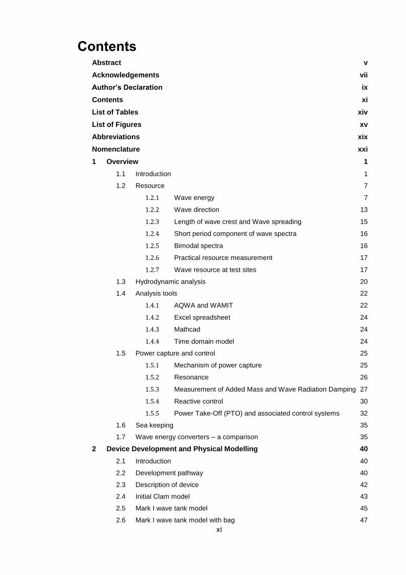
Contents Abstract v

Acknowledgements vii

Author’s Declaration ix

Contents xi

List of Tables xiv

List of Figures xv

Abbreviations xix

Nomenclature xxi

1 Overview 1

1.1 Introduction 1

1.2 Resource 7

1.2.1 Wave energy 7

1.2.2 Wave direction 13

1.2.3 Length of wave crest and Wave spreading 15

1.2.4 Short period component of wave spectra 16

1.2.5 Bimodal spectra 16

1.2.6 Practical resource measurement 17

1.2.7 Wave resource at test sites 17

1.3 Hydrodynamic analysis 20

1.4 Analysis tools 22

1.4.1 AQWA and WAMIT 22

1.4.2 Excel spreadsheet 24

1.4.3 Mathcad 24

1.4.4 Time domain model 24

1.5 Power capture and control 25

1.5.1 Mechanism of power capture 25

1.5.2 Resonance 26

1.5.3 Measurement of Added Mass and Wave Radiation Damping 27

1.5.4 Reactive control 30

1.5.5 Power Take-Off (PTO) and associated control systems 32

1.6 Sea keeping 35

1.7 Wave energy converters – a comparison 35

2 Device Development and Physical Modelling 40

2.1 Introduction 40

2.2 Development pathway 40

2.3 Description of device 42

2.4 Initial Clam model 43

2.5 Mark I wave tank model 45

2.6 Mark I wave tank model with bag 47

xii

2.6.1 Air compressibility 47

2.6.2 Losses in connecting pipework 48

2.6.3 Building a leak-tight system 48

2.7 Design and construction of Mark IIa wave tank model 49

2.7.1 Main assembly 49

2.7.2 Flexible bag 51

2.7.3 Hinge 52

2.7.4 Power Take-Off (PTO) 53

2.7.5 Ballast 56

2.7.6 Mass properties: 58

2.8 Mark IIb wave tank model 60

2.8.1 Description of modification 60

3 Mathematical Modelling 62

3.1 General 62

3.2 Resonant period and heave stability 62

3.2.1 Resonant period 62

3.2.2 Heave stability 64

3.3 AQWA/WAMIT verification 65

3.4 Generalised Mode applied to Clam action 70

3.5 WAMIT analysis 74

3.6 Frequency domain model 75

3.7 Free floating Clam - regular input 80

3.8 Heave restrained Clam - regular input 82

3.9 Free floating versus heave restrained configurations 84

3.10 Performance with random input 84

3.11 Time domain model description 86

3.11.1 General 86

3.11.2 PTO and Heave Stiffness & Damping 87

3.11.3 Integration engine 90

3.11.4 Equations of motion 90

3.11.5 Coulomb friction 90

3.11.6 Wave generation and excitation 91

3.11.7 Use of Convolution Integral 92

4 Wave Tank Trials and Analysis 95

4.1 Introduction 95

4.2 Test facilities at Plymouth 95

4.3 Test setup for trials of Mark IIa model 97

4.4 Test setup for trials of Mark IIb model 100

4.5 Trials programme 103

4.5.1 Trial 1 - Floating, Rigid body 106

4.5.2 Trial 2 - Floating Clam 108

xiii

4.5.3 Trial 3 - No heave, 40 mm wave input 110

4.5.4 Trial 4 – No Heave, 20 mm wave input, coil spring 112

4.5.5 Trial 5 – 20mm wave, constant force spring, 5 mm orifice 113

4.5.6 Trial 6 – 20mm wave, constant force spring, 3 mm orifice 115

4.5.7 Trial 7 – 20mm wave, constant force spring, 2.5 mm orifice 116

4.5.8 Variation of power capture with wave input angle 117

4.5.9 Time domain modelling – Trial 7 119

4.5.10 Performance in random seas 121

4.5.11 Performance in random seas with spread 125

4.6 Discussion of trial results 126

5 Full Scale Design 136

5.1 Introduction 136

5.2 Main Features of the proposed design concept 136

5.3 Performance prediction 136

6 Conclusions and Suggestions for further research 141

6.1 Aim of the research 141

6.2 Conclusions reached 141

6.3 Suggestions for further research and development 143

References 145

Appendix A: Scaling Factors 151

Appendix B: WAMIT modelling 152

B.1 General 152

B.2 Model Control Files 152

B.3 Geometry definition 153

B.4 Force Control file 154

B.5 NEWMODES data file 156

B.6 Output from WAMIT model 156

Appendix C: Trials carried out 157

Appendix D: Power Capture at Wave Hub 160

xiv

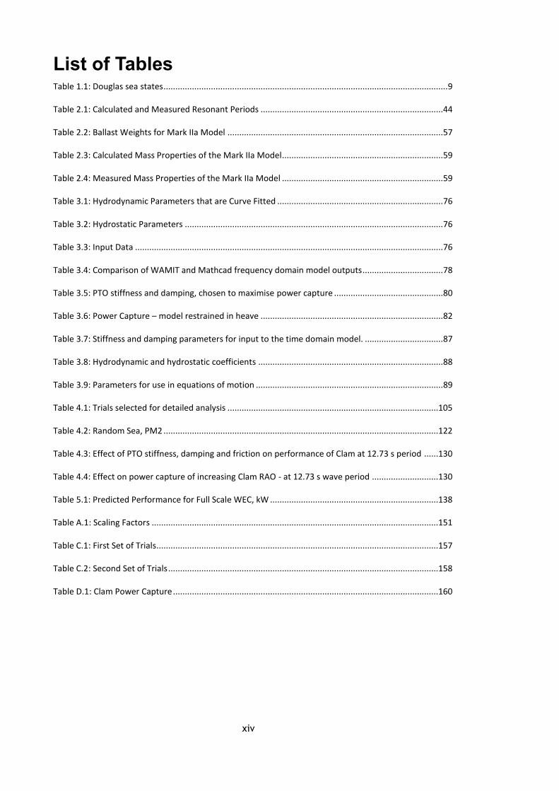
List of Tables Table ‎1.1: Douglas sea states ........................................................................................................................ 9

Table ‎2.1: Calculated and Measured Resonant Periods ............................................................................. 44

Table ‎2.2: Ballast Weights for Mark IIa Model ........................................................................................... 57

Table ‎2.3: Calculated Mass Properties of the Mark IIa Model.................................................................... 59

Table ‎2.4: Measured Mass Properties of the Mark IIa Model .................................................................... 59

Table ‎3.1: Hydrodynamic Parameters that are Curve Fitted ...................................................................... 76

Table ‎3.2: Hydrostatic Parameters ............................................................................................................. 76

Table ‎3.3: Input Data .................................................................................................................................. 76

Table ‎3.4: Comparison of WAMIT and Mathcad frequency domain model outputs .................................. 78

Table ‎3.5: PTO stiffness and damping, chosen to maximise power capture .............................................. 80

Table ‎3.6: Power Capture – model restrained in heave ............................................................................. 82

Table ‎3.7: Stiffness and damping parameters for input to the time domain model. ................................. 87

Table ‎3.8: Hydrodynamic and hydrostatic coefficients .............................................................................. 88

Table ‎3.9: Parameters for use in equations of motion ............................................................................... 89

Table ‎4.1: Trials selected for detailed analysis .........................................................................................105

Table ‎4.2: Random Sea, PM2 ....................................................................................................................122

Table ‎4.3: Effect of PTO stiffness, damping and friction on performance of Clam at 12.73 s period ......130

Table ‎4.4: Effect on power capture of increasing Clam RAO - at 12.73 s wave period ............................130

Table ‎5.1: Predicted Performance for Full Scale WEC, kW .......................................................................138

Table A.1: Scaling Factors .........................................................................................................................151

Table C.1: First Set of Trials.......................................................................................................................157

Table C.2: Second Set of Trials ..................................................................................................................158

Table D.1: Clam Power Capture ................................................................................................................160

xv

List of Figures

Figure ‎1.1: Wave Power Levels in kW/m Crest Length (Cornett, 2008) ....................................................... 7

Figure ‎1.2: Power Spectrum of typical sea state(Shaw, 1982) ..................................................................... 8

Figure ‎1.3: South Uist Scatter diagram 1976/77 (occurrence in parts per thousand) (Dawson, 1979) . 13

Figure ‎1.4: Wave Power Rose at the offshore buoy (Iglesias & Carballo, 2011) ........................................ 14

Figure ‎1.5: Directional Spectra at the Wave Hub Test site (Saulnier, Maisondieu, et al., 2011) ............... 14

Figure ‎1.6: Tightening of directional spectra due to shoaling (Henry, 2010) ............................................. 15

Figure ‎1.7: Modes of energy absorption (Falnes, 2002) ............................................................................ 26

Figure ‎1.8: Destructive wave patterns for a heaving point absorber (Falnes, 2002) ................................. 27

Figure ‎1.9: Under-Damped Oscillations ..................................................................................................... 29

Figure ‎1.10: Under-Damped Oscillations – Logarithmic Decrement .......................................................... 29

Figure ‎1.11: Resonance and phase control (Falnes, 2005) ......................................................................... 30

Figure ‎1.12: Phase and Latching Control – a comparison (Falnes, 2005) ................................................... 31

Figure ‎1.13: Heaving Point Absorber with Hydraulic PTO (Falcão, 2005) .................................................. 33

Figure ‎1.14: 1:9 Scale model of the AWS-III under test on Loch Ness, June 2010 ..................................... 38

Figure ‎2.1: Free Floating Clam (Farley, 2011c) ........................................................................................... 42

Figure ‎2.2: Initial Clam Model .................................................................................................................... 44

Figure ‎2.3: Mark I Wave Tank Model – Cross Section ................................................................................ 45

Figure ‎2.4: Mark I Wave Tank Model with keel.......................................................................................... 46

Figure ‎2.5: Mark I Wave Tank Model plus bag in Plymouth Laboratory .................................................... 47

Figure ‎2.6: Basic Geometry of Mark IIa Wave Tank Model ........................................................................ 49

Figure ‎2.7: Mark IIa Wave Tank Model ready for testing ........................................................................... 50

Figure ‎2.8: CAD model of Mark IIa Wave Tank Model ............................................................................... 50

Figure ‎2.9: Flexible bag for Clam ................................................................................................................ 51

Figure ‎2.10: Hinge Assembly ...................................................................................................................... 52

Figure ‎2.11: Power Take-Off Schematic ..................................................................................................... 53

Figure ‎2.12: Clam Model - floating ............................................................................................................. 54

xvi

Figure ‎2.13: Power Take-Off Assembly ....................................................................................................... 55

Figure ‎2.14: Power Take-Off Base Assembly .............................................................................................. 55

Figure ‎2.15: Orifice Plate ............................................................................................................................ 56

Figure ‎2.16: Strut ........................................................................................................................................ 56

Figure ‎2.17: Ballast Weights for Clam ......................................................................................................... 57

Figure ‎2.18: Ballast Weight Positions ......................................................................................................... 58

Figure ‎2.19: Mark IIb_1, Model with coil springs fitted .............................................................................. 61

Figure ‎2.20: Mark IIb_2, Model with constant force springs fitted ............................................................ 61

Figure ‎3.1: Clam Geometry ......................................................................................................................... 62

Figure ‎3.2: Wave Tank Model Geometry for Hydrodynamic Analyses ....................................................... 66

Figure ‎3.3: AQWA Wave Tank Model – without uprights ........................................................................... 66

Figure ‎3.4: AQWA/WAMIT Heave Added Mass Comparison ...................................................................... 67

Figure ‎3.5: AQWA/WAMIT Heave Radiation Damping Comparison ........................................................... 67

Figure ‎3.6: AQWA Wave Tank Model – with uprights ................................................................................ 68

Figure ‎3.7: AQWA Wave Tank Model comparison – Added Mass .............................................................. 69

Figure ‎3.8: AQWA Wave Tank Model comparison – Radiation Damping ................................................... 69

Figure ‎3.9: Definition of Mode 7 ................................................................................................................. 70

Figure ‎3.10: Incorrectly predicted Clam response ...................................................................................... 73

Figure ‎3.11: Improved prediction of Clam response .................................................................................. 73

Figure ‎3.12: Power Capture for Free Floating device - 1 ............................................................................ 81

Figure ‎3.13: Power Capture for Free Floating device - 2 ........................................................................... 81

Figure ‎3.14: Power Capture – model restrained in heave - 1 ..................................................................... 83

Figure ‎3.15: Power Capture for model restrained in heave – 2.................................................................. 83

Figure ‎3.16: Power Capture Comparison – free floating versus heave mode ............................................ 84

Figure ‎3.17: Time domain model - Top level Block Diagram ...................................................................... 87

Figure ‎4.1: Initial Mooring Geometry for the First set of trials ................................................................... 98

Figure ‎4.2: First Modification to the Mooring Geometry for the First set of trials..................................... 98

Figure ‎4.3: Final Modification to the Mooring Geometry for the First set of trials .................................... 99

Figure ‎4.4: Mooring Geometry for Second set of trials ............................................................................100

xvii

Figure ‎4.5: Plan View of Wave Gauge Positions for Second set of trials .................................................. 101

Figure ‎4.6: Wave gauge readings for a wave incident angle of 0° - trial 7 ............................................... 102

Figure ‎4.7: Wave gauge readings for a wave incident angle of 15° - trial 7 ............................................. 102

Figure ‎4.8: Wave gauge readings for a wave incident angle of 30° - trial 7 ............................................. 103

Figure ‎4.9: Heave RAO and Phase, Fixed Clam, Trial 1 ............................................................................. 107

Figure ‎4.10: Amplitude of PTO Load, Fixed Clam, Trial 1 ......................................................................... 107

Figure ‎4.11: Heave RAO and Phase, Trial 2 .............................................................................................. 109

Figure ‎4.12: RAO and Phase for PTO, Trial 2 ............................................................................................ 109

Figure ‎4.13: Load in Model PTO, Trial 2 ................................................................................................... 109

Figure ‎4.14: Power Capture, Trial 2, (a) model scale, (b) full scale .......................................................... 110

Figure ‎4.15: Heave RAO and Phase, Trial 3 .............................................................................................. 111

Figure ‎4.16: PTO RAO and Phase Lag, Trial 3 ........................................................................................... 111


Figure ‎4.18: Load in Model PTO, Trial 3 ................................................................................................... 112

Figure ‎4.19: RAO, Phase Lag and Load Amplitude in Model PTO, Trial 4 ................................................. 112




Figure ‎4.23: RAO, Phase Lag and Load Amplitude in Model PTO, Trial 6, (a) model scale, (b) full scale . 115




Figure ‎4.27: Power Capture variation with wave angle; model configured as for Trial 5 ........................ 117

Figure ‎4.28: Power Capture variation with wave angle; model configured as for Trial 7 ........................ 118

Figure ‎4.29: Wave Tank Data - Trial 7, Run 5 ........................................................................................... 119

Figure ‎4.30: Time domain model simulation - Trial 7, Run 5 ................................................................... 119

Figure ‎4.31: Comparison between Calculated and Measured PTO Displacement - Trial 7, Run 5........... 120

Figure ‎4.32: Comparison between Calculated and Measured PTO Load - Trial 7, Run 5 ......................... 120

Figure ‎4.33: Measured PSD for Trial 20 compared with smooth spectrum used for analysis ................ 121

xviii

Figure ‎4.34: Wave Tank Data – Random Seas, PM2 .................................................................................123

Figure ‎4.35: Time domain model simulation - Random Seas, PM2 ..........................................................123

Figure ‎4.36: Comparison between Calculated and Measured PTO Displacement - Random Seas, PM2 .124

Figure ‎4.37: Comparison between Calculated and Measured PTO Load - Random Seas, PM2 ...............124

Figure ‎4.38: Resonant Period of Clam mode ............................................................................................128

Figure ‎4.39: Capture width versus PTO RAO ............................................................................................131

Figure ‎4.40: Power prediction accuracy ...................................................................................................132

Figure ‎4.41:‎Comparison‎of‎Clam’s‎Performance‎with‎Floating‎Oscillating‎Water‎Column‎WEC .............133

Figure ‎4.42: "Annual Average" Wave Input Spectrum at Benbecula (Phillips & Rainey, 2005) ................134

Figure ‎5.1: Surface Plot of interpolated power capture values ................................................................138

Figure ‎5.2: Joint probabilities, Hm0 (Hs) and Tm-1,0 (Te) at Wave Hub, locn 1 (Nieuwkoop et al.), 2013) 139

Figure ‎5.3, Mean Wave Pwr (kW/m) binned by wave dirn (°N) at Wave Hub (Nieuwkoop et al.), 2013) 139

Figure B.1: Input parameters for Newmodes.f .........................................................................................156

xix

Abbreviations AMETS

Atlantic Marine Energy Test Site

AQWA

A computing environment for hydrodynamic analysis

AWS

Archimedes Wave Swing

CAD

Computer Aided Design

CG Centre of Gravity

CL Centreline

CT Carbon Trust

DanWEC Danish Wave Energy Centre

DFIG

Doubly-Fed Induction Generator

DoE Department of Energy

ETSU

Energy Technology Support Unit

FORTRAN

A general-purpose programming language, from “Formula

Translation”

HF

High Frequency

HMRC

Hydraulic & Maritime Research Centre

IRF Impulse Response Function

JONSWAP

Joint North Sea Wave Project

MASK Manoeuvering and Seakeeping Basin, Maryland

MATLAB

A computing environment, formerly “matrix laboratory”

MCT

Marine Current Turbines

MEA

Marine Energy Accelerator

MEC

Marine Energy Challenge

MILDwave

An in-house numerical model from Ghent University

MIT

Massachusetts Institute of Technology

xx

MS EXCEL

Microsoft Excel – a spread sheet programme

NCEP

National Centers for Environmental Prediction

NDBC

National Data Buoy Center

NEL

National Engineering Laboratory

NOAA

National Oceanic and Atmospheric Administration

OWC

Oscillating Water Column

OWSC

Oscillating Wave Surge Converter

p/kWh

Pence per kilowatt hour

PC

Personal Computer

PTC

A software company, formerly Parametric Technology Corporation

PTO

Power Take-Off (PTO)

RAO

Response Amplitude Operator

RD&D

Research, Development and Demonstration

RHM

Reactive Hydraulic Modulator

SEA Ltd

Systems Engineering and Assessment Ltd

SHM

Simple Harmonic Motion

SPERBOY

Sea Power Energy Recovery Buoy

UK

United Kingdom

WAM

Wave Analysis Model

WAMDI

Wave Model Development and Implementation

WAMIT

Wave Analysis MIT

WEC

Wave Energy Converter

WES

Wave Energy Scotland

WW3

WAVEWATCH III

xxi

Nomenclature

𝑎 Wave amplitude

𝐴 Area

𝐴 Amplitude

𝐴 Parameter equal to 𝐻𝑠2/4𝜋𝑇𝑧

4

𝐴33 Heave Added Mass

𝐴37 Cross coupled (3,7) Added Mass

𝐴73 Cross coupled (7,3) Added Mass

𝐴77 Clam mode Added Mass

𝐴𝑖𝑗 Element in the hydrodynamic added mass matrix, 𝐴

𝐵 Parameter equal to 1/𝜋𝑇𝑧4

𝑏 Damping

𝐵33 Heave hydrodynamic damping

𝑏33 Heave hydrodynamic damping, 𝐵33, + externally applied heave damping, 𝐵33𝐸

𝐵33𝐸 Externally applied heave damping

𝐵37 Cross coupled (3,7) hydrodynamic damping

𝑏37 Cross coupled (3,7) hydrodynamic damping (= 𝐵37)

𝐵73 Cross coupled (7,3) hydrodynamic damping

𝑏73 Cross coupled (7,3) hydrodynamic damping (= 𝐵73)

𝐵77 Clam mode hydrodynamic damping

𝑏77 PTO mode hydrodynamic damping, 𝐵77, + externally applied PTO (=Clam mode)

mode, 𝐵77𝐸

𝐵77𝐸 PTO (= Clam mode) damping

𝐵𝑖𝑗 Element in the hydrodynamic damping matrix, 𝐵

𝐵𝑖𝑗𝐸 Element in the external damping matrix, 𝐵𝐸

𝐶 Damping

𝑐 Damping

C(𝑠) Normalising factor

𝐶33 Heave hydrostatic coefficient

𝑐33 Hydrostatic stiffness, 𝐶33 + externally applied heave stiffness, 𝐶33

𝐸

𝐶33𝐸 Externally applied heave stiffness

xxii

𝐶37 Cross coupled (3,7) hydrostatic coefficient

𝑐37 Cross coupled (3,7) hydrostatic coefficient, 𝐶37

𝐶73 Cross coupled (7,3) hydrostatic coefficient

𝑐73 Cross coupled (7,3) hydrostatic coefficient, 𝐶73

𝐶77 Clam mode hydrostatic coefficient

𝑐77 Clam hydrostatic stiffness 𝐶77 + externally applied Clam mode stiffness (= PTO

stiffness), 𝐶77𝐸

𝐶77𝐸 Clam mode stiffness (= PTO stiffness)

𝐶𝐷 Drag coefficient

𝐶𝑖𝑗 Hydrostatic Coefficient - Element in the hydrostatic stiffness matrix, 𝐶

𝐶𝑖𝑗𝐸 Element in the external stiffness matrix, 𝐶𝐸

𝐷 Duration of record

𝐷(𝑓, 𝜃) Angular spreading function

𝑓 Wave frequency

𝑓(𝑡) Excitation Impulse Response Function (IRF)

F PTO Force

𝐹𝐶𝐷 Coulomb damping force

𝐹𝐶𝐹 Coulomb friction force

𝑓𝑛 Wave frequency for index 𝑛

Fb Buoyancy force

FS Spring force

𝐹𝐷 Component of PTO force due to damping

𝐹𝑒(𝑡) Excitation force

Fw Wave force

𝑔 Acceleration due to gravity

G Acceleration due to gravity

ℎ Height of Clam side

𝐻13⁄ Significant wave height

𝐻𝑠 Significant wave height

𝑖 Imaginary number (= √−1) – used in complex number notation

𝑗 Imaginary number (= √−1) – used in complex number notation

xxiii

𝐼𝑚𝑋3 Imaginary part of complex heave excitation force

𝐼𝑚{𝐹𝑒(𝜔)} Imaginary part of the Excitation Force in the frequency domain.

𝑘 Stiffness

𝑘′ Stiffness

𝑘(𝑡) Radiation Impulse Response Function (IRF)

L Length of Clam side

M Mass

𝑚 Mass of the buoy

ma Hydrodynamic added mass

𝑚𝑚 Mass of body

𝑚(𝜔) Hydrodynamic added mass

𝑚(∞) Body added mass as wave frequency tends to infinity (i.e. at zero wave period)

𝑀33 Device mass

𝑚33 Body mass, 𝑀33+ heave Added Mass, 𝐴33

𝑚37 Cross coupled (3,7) Added Mass (= 𝐴37)

𝑚73 Cross coupled (7,3) Added Mass (= 𝐴73)

𝑚77 Hydrodynamic added mass for PTO mode (= 𝐴77)

𝑀𝑖𝑗 Element in the mass and inertia matrix, 𝑀

𝑀𝑖𝑗𝐸 Element in the external mass and inertia matrix, 𝑀𝐸

𝑀𝑛 nth

spectral moment

𝑀𝑜𝑑33 Modulus of Haskinds Exciting Force in Heave

𝑀𝑜𝑑77 Modulus of Haskinds Exciting Force for Clam Mode

𝑛 Integer index

𝑛 Number of sample values taken of 𝑦𝑖 – an integer

𝑛𝑧 Number of times the water surface moves through its mean level in the upward direction

𝑁 Maximum number of steps

𝑃𝑤𝑎𝑣𝑒 Power per unit width of wave crest

𝑃𝑚 Mean power absorbed by the PTO

𝑃 Power Capture,

𝑃𝑤 Power absorbed from the waves

xxiv

Periodj Wave period in seconds

𝑃𝑆𝐷 Power spectral density

𝑅𝐴𝑂 Response Amplitude Operator

𝑅𝐴𝑂3 Heave RAO

𝑅𝐴𝑂7 PTO RAO

𝑅𝑒𝑋3 Real part of complex heave excitation force

𝑅𝑒{𝐹𝑒(𝜔)} Real part of the Excitation Force in the frequency domain

𝑅𝑞 Quadratic damping coefficient

𝑅(𝜔) Radiation damping

s Spreading value

𝑆 Externally applied stiffness

𝑆𝑏 Hydrostatic stiffness

𝑠(𝑡) Body vertical position

𝑆(𝑓) One-dimensional wave spectrum (or ‘power spectral density function’)

𝑆(𝑓, 𝜃) Directional wave spectrum

𝑆(𝑓𝑛) Wave input spectrum at the wave frequency 𝑓𝑛

Sj Spectrum used in the frequency domain analysis

T Resonant Period

T Sampling interval

𝑡 Time

𝑇 Wave Period

𝑇13⁄ Significant Period

𝑇0 Undamped resonant period (=

2𝜋

𝜔0 )

𝑇𝑒 Energy Period

𝑇𝑛 Wave period for index 𝑛

𝑇𝑧 Zero Crossing Period

𝑈 Wind speed at 19.6 m above sea level (ms-1

)

𝑈 Velocity

𝑢(𝑡) Body vertical velocity

�̇�(𝑡) Body vertical acceleration

xxv

VELH Displacement normal to the surface (+ve into the body)

w Wave position

𝑊 Width of the WEC/buoy

𝑊𝑐 Capture Width

𝑥 Buoy displacement

𝑥 Length of spring

𝑥, 𝑦 and 𝑧 Cartesian coordinates.

𝑥1 , 𝑥2 Successive peaks in logarithmic decay record

𝑋3 Wave excitation force in heave (mode 3)

𝑋7 Wave excitation force in clam mode (mode 7)

𝑋𝑖 Exciting force in the ith

mode

Y Water level

𝑦𝑖 Water level at instant, 𝑖 , relative to the mean water level

𝑍 Vertical distance from the Clam pivot to the line of action of the PTO ram,

𝑍33 Complex stiffness, heave mode

𝑍37 Complex stiffness, cross-coupled mode (3,7)

𝑍73 Complex stiffness, cross-coupled mode (7,3)

𝑍77 Complex stiffness, clam mode

𝑧, �̇�, �̈� Vertical displacement, velocity and acceleration of buoy

ZDISP Vertical (Z-direction) displacement

𝛤 Gamma function

𝛿 Intermediate parameter in calculation of 𝜁

𝛿 Logarithmic decrement

�̇�3 Heave velocity

�̈�3 Heave acceleration

�̇�7 PTO velocity

�̈�7 . PTO acceleration

𝛿3 Heave position

𝛿7 PTO position

∆𝑓 Small frequency interval at frequency 𝑓

xxvi

∆𝑓𝑛 Step size in wave frequency, equivalent to step size 𝑇𝑛 in Wave period

∆𝑃𝑛 Incremental contribution to power capture over frequency step, ∆𝑓𝑛

∆𝑇 Step size in time

𝜁 Damping ratio

𝜂(𝑡) Wave Position (in relation to mean)

𝜃 Angular difference between the wave direction and the mean wind direction

𝜃 Clam semi-angle

𝜉7 Complex PTO amplitude

𝜉𝑗 Displacement in the jth

degree of freedom (or mode) caused by the force 𝑋𝑖

𝜋 Ratio of a circle's circumference to its diameter

𝜌 Density of water

𝜎 Root mean square value of the water level relative to the mean water level

𝜎2 Mean square value

𝜎33 Argument of Haskinds Exciting Force in Heave

𝜎33 Phase lag in mode 3 (heave)

𝜎77 Argument of Haskinds Exciting Force for Clam Mode

𝜎77 Phase lag in mode 7 (clam mode)

𝜏 Time before current time

𝜑 Velocity Potential

𝜔 Wave radian frequency (=2𝜋

𝑊𝑎𝑣𝑒 𝑃𝑒𝑟𝑖𝑜𝑑)

𝜔0 Undamped resonant frequency

|𝜉3| Modulus of the heave amplitude

|𝜉7| Modulus of the PTO (mode 7) amplitude

1

1 Overview

1.1 Introduction

Marine energy, and particularly wave energy has the potential to provide a substantial

proportion of the UK and global energy requirement. For example in 1982 the realisable

UK potential for wave energy was estimated to be 20% of UK electrical energy demand,

some 5 GW of a total mean UK requirement of 25 GW (Shaw, 1982). Tidal stream turbine

installations were estimated to be capable of providing 1.8 GW, while the Severn Barrage

scheme could provide a further 2 GW, some 5% of UK demand.

In the few years prior to 1982 UK research into wave energy had received the largest share

of renewables funding. In 1978 Research, Development and Demonstration (RD&D)

programmes in wave energy received £5.4 M which was increased to £13.1 M by June

1981. In 1981 contracts were awarded to Edinburgh University for work on the spine

structure for the ‘Salter Duck’ and wave tank development, to Vickers for oscillating water

column development, to Sea Energy Associates for spine and mooring systems and to Sir

Robert McAlpine for the Bristol Cylinder development. Unfortunately in 1982 the

government decided to abandon support for wave power in favour of conventional sources.

Final curtailment followed publication of "Wave Energy, ETSU R26" in March 1985 (DoE

UK, 1985). Acrimony surrounded the decision and it was believed that the conclusions

were based on invalid assumptions (Wilson, 2010). Although large scale funding was

curtailed the ETSU report (DoE UK, 1985) suggested funding for research should continue

and in particular small scale versions of both the CLAM device of SEA Ltd and the NEL

Breakwater device were supported by the Department of Energy. The Edinburgh DUCK

received special attention in the report since it was far and away the most efficient device

tested. The methodology for assessing the various devices involved scoring the various

attributes of each device in order to arrive at an overall score. On account of its complexity

the DUCK scored so low in regards to its estimated availability that the engineering

problems “prevented the Consultants from carrying out their assessment”. It is interesting

to make the comparison with the Pelamis wave energy converter (WEC), also complicated

and also from the Edinburgh stable. However, as will be seen from the work on the Floating

2

Clam reported here, a degree of complexity is required in order to achieve an acceptable

level of power capture. The ETSU report (DoE UK, 1985) highlighted the potential for small

scale use of wave power in particular cases such as when integrated with breakwaters.

Thus continued small scale development of wave power was encouraged. Research

continued in the UK, notably Edinburgh and in other countries including Norway.

Research into renewable sources of energy was initially driven by the realisation that

ultimately fossil fuels would run out. However in the light of an increasing awareness of the

threat of global warming RD&D into renewable technologies then received increasing UK

government support and in 2005 eight off-shore devices were chosen to take part in the

Carbon Trust’s Marine Energy Challenge (MEC). The developers were Clearpower

Technologies (WaveBob), Ocean Power Delivery (Pelamis), SeaVolt Technologies (Wave

Rider), AquaEnergy (AquaBuOY), Lancaster University (PS Frog), Evelop (Wave Rotor),

Embley Energy (Sperboy) and Wave Dragon. The MEC also included discrete work

packages such as shoreline OWC, tidal stream, and marine energy design codes and

standards to supplement the direct technology assessment. The programme was launched

amid great optimism. In the launch press release of 11th February 2004 Tom Delay, Chief

Executive of the Carbon Trust, commented: “As yet no country has taken a leading position

in marine energy. A relatively small investment now could make a significant impact to the

UK’s competitive position due to the early-stage of technology development”.

Naturally wave energy devices require test facilities, from small scale testing in a wave

tank, through to sea-going prototypes. The UK is well placed to support these activities

which have received appropriate government support. Of particular note in the context of

wave energy development are the wave tanks at Edinburgh and Plymouth Universities.

Ocean test sites include the European Marine Energy Centre (EMEC) based at Stromness

in Orkney and Wave Hub Ltd in Cornwall. This latter company operates two wave energy

test sites, the Pembrokeshire Demonstration Zone and Wave Hub which is off the North

Coast of Cornwall. Wave Hub would be the obvious choice to test a prototype arising from

the present work.

3

Events have shown that wave power has some way to go in becoming commercially viable.

Of the eight developers that were chosen to take part in the Marine Energy Challenge,

none are still active. The developers of Wave Bob and Pelamis have gone into liquidation,

and an AquaBuoy prototype sank in 2007 - development appears to not to have been

continued. Internet searches result in virtually no trace of Wave Rotor, while the

development of both SPERBOY and Wave Dragon appears to have ceased, at least

temporarily.

Nevertheless optimism as to the future of wave energy has continued. In the UK the

Carbon Trust (CT) has been a major supporter of wave energy development and has

helped the industry by means of a number of initiatives. Between 2003 and 2011 the CT

had invested £30M in the marine energy industry. CT’s Marine Energy Accelerator (MEA)

programme, which ran from 2007 to 2010 was designed to achieve reductions in the cost of

energy produced. The MEA aimed to gain an understanding of the potential of cost of

energy reduction through targeted innovation, working with existing device concepts to

develop a set of cost reductions. The MEA programme also included support for new

device concepts to explore the potential for a single step change in cost of energy. The

MEA report (Carbon Trust, 2011) considered that in the case of wave energy, sufficient

improvements in performance, produceability, survivability, structural design etc. would

come through gradual improvements in accordance with normal established “learning

curves”, albeit with some targeted accelerated cost reduction techniques. Both wave and

tidal power energy costs were predicted to reduce from 35 or 40 p/kWh - to equivalence

with offshore wind at 13 or 14 p/kWh over the fifteen year period, from 2010 to 2025. Case

studies undertaken within the MEA programme included an innovative linear generator for

future wave energy devices (Edinburgh University) and the development of installation and

connection equipment for Pelamis to enable operations in bigger seas, and faster

deployment. Checkmate Sea Energy also received funding for the promising innovative

concept, Anaconda.

In addition the Marine Renewables Proving Fund was set up and managed by the Carbon

Trust during 2009 to 2011 to provide financial and technical support for the demonstration

4

of promising wave and tidal devices. Six developers were selected for support. These

were Aquamarine Power (Oyster - wave), Atlantis Resources Corporation (Atlantis - tidal),

Pelamis Wave Power (Pelamis - wave), Voith Hydro Ocean Current Technologies (Voith -

tidal), Hammerfest Strom UK (HS-1000 - tidal) and Marine Current Turbines (MCT – tidal).

Just two of these six developers were involved in wave power and both have failed

financially. The remaining four developers were in tidal power. Two of them (MCT and

Atlantis) are now owned by them same company (Atlantis). ANDRITZ HYDRO Hammerfest

Strom is part of ANDRITZ, which is a global and stock exchange listed technology Group

with more than 17,000 employees. No reference to tidal power can be found on the Voith

website. According to the information on the CT web site the scheme has proved that “full

scale marine energy devices can be installed and operated in open-sea environments”

(Carbon Trust, 2016). Thus for tidal power the technology is maturing fast and market

leaders in the form of large international companies are emerging. However, in view of the

fact that both of the front runners, Pelamis and Oyster have failed financially, this can

hardly be said to be true for wave power.

Nevertheless, support continues for wave power development. The Scottish government,

through Wave Energy Scotland (WES) (WES, 2016b) stepped in following the demise of

Pelamis and Oyster by purchasing the intellectual property and some of the hardware. It is

hoped that buyers will be found for what can be salvaged. In parallel, WES launched fresh

initiatives to support the industry with two funding calls. The first supported innovations in

Power Take-Off (PTO) technology while the second was for Novel Wave Energy

Converters (WES, 2016a). These calls provided up to 100% funding to encourage

innovation and enable the wave power industry to become a cost effective generator of

electricity. The long term cost (50 years hence) for wave power generated electricity is put

at only 2 p/kWh at present price levels (Carbon Trust, 2006). Whether this is achievable

remains to be seen. However it is interesting to note that onshore wind power is now the

least expensive form of electrical energy in the UK. In 2015 the price of onshore wind

generated electricity was 5.53 p/kWh, which compared with 7.4 p/kWh for electricity from

coal or gas (Bawden, 2015).

5

In the USA wave energy is receiving increased support under the “Wave Energy Prize”

scheme (Anon, 2016) which is part of the US Department of Energy’s Water Power

Programme. The aim is to attract next generation ideas by offering a prize purse and

providing an opportunity for testing at the US’s most advanced wave-making facility, the

Naval Surface Warfare Center Carderock’s Maneuvering and Seakeeping (MASK) Basin in

Maryland. The assessment process began with model testing at a scale of 1:50 and a

proof of concept assessment by an expert panel. As a result 11 teams have been chosen

to take part in the final stage which includes wave tank trials at a scale of 1:20. Grants are

given to participants towards the cost of model construction, testing etc. The developers of

the most promising devices will receive prizes, a first prize of - $1,500,000, a second prize

of $500,000 and a third prize of $250,000.

The writer became involved in wave energy as a spare-time interest in 1997 by providing a

mathematical simulation model for Rod Youlton, the inventor of SPERBOYTM

, the floating

oscillating water column WEC. In 1998 funding was secured by the University of Plymouth

from The European Commission within the Non Nuclear Energy Programme JOULE III for

research funding for SPERBOY, and a 1/5th size pilot device was deployed south of

Plymouth Sound in 2001. Unfortunately this was irreparably damaged in a storm after only

10 days of testing. Having been involved through SPERBOY in the Marine Energy

Challenge, the writer then led a study entitled 'Advanced Concrete Structural Design of the

SPERBOY Wave Energy Converter’, which was supported by the Carbon Trust and the

nPower Juice Fund. This showed a delivered cost of electricity of 16 p/kWh based on a

15% discount rate and a 20 year life – the standard conditions used by the CT for device

assessment.

In 2010 the writer was fortunate to be accepted for a self-funded programme of research at

the University of Plymouth. Initially this was to be an optimisation study of the SPERBOY

type of WEC – a floating oscillating water column device. However, the opportunity

presented itself to work on a promising novel concept which Francis Farley (Farley, 2011d)

had patented. Thus the Floating Clam was taken as the basic concept around which this

study revolves. The basis of the concept as originally conceived was to use “Clam action”

6

to lengthen the resonant period – as compared to that of a rigid body. In addition the Power

Take-Off (PTO) was contained entirely with the structure, thus avoiding contamination and

hazards from sea-borne debris etc. In the process of testing the Floating Clam it has been

found that wide-band energy capture would result from restraining the Clam in heave.

Tuning the heave response in the way originally conceived has in the final analysis not

proved beneficial – for discussion on this point see Section ‎2.3.

Whether the Floating Clam will be prove to be a successful device remains to be seen. It

may well join the long list of promising and not-so-promising devices. A recent study

compares a total of 175 mostly unsuccessful devices (Joubert et al., 2013).

The one parameter that feeds directly into any calculation of the cost of generated

electricity is the efficiency of power capture itself – and this is the main topic of interest in

the present study. It will be shown that the Floating Clam is particularly efficient in this

regard but that the full-scale embodiment of the technology is challenging. Whereas the

device, as described in the patent is designed to employ an air turbine generator,

alternative PTO methods are possible. A promising and innovative method of power take

off is the Capstan Drive as discussed in the final chapter.

This document presents the reader in the first chapter with the theoretical basis on which

the subsequent analyses depend. Then in Chapter 2 the wave tank models are described.

Chapter 3 describes the mathematical models that have been developed to predict device

behaviour and power capture performance while Chapter 4 covers the practical testing and

its analysis. Chapter ‎5 presents an estimate of the performance that might be expected of

a full scale device at a specific location - the Wave Hub test site in Cornwall Finally

Chapter 6 draws conclusions and makes suggestions for further work

7

1.2 Resource

1.2.1 Wave energy

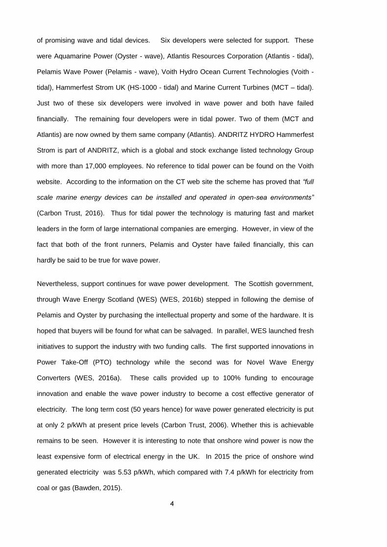
A convenient measure of the wave energy availability at a specific site is the annual

average power per metre of wave front. Figure ‎1.1 shows the global wave energy

availability, measured in kW/m (Cornett, 2008).

Figure ‎1.1: Wave Power Levels in kW/m Crest Length (Cornett, 2008)

The waves in real seas are random, varying in height, period and direction. However, for

analysis purposes they can be considered to be made up of a combination of “regular”

waves, each moving with simple harmonic motion. The mathematical analysis of these

simple waves was solved in the early part of the 19th century (Stokes, 1847). A review of

Stokes’ work is contained in the paper by Craik (2005).

The profile of the water surface in a regular wave is close to being a sine wave – and in

deep water it is so. For this case the power per unit width of wave crest, 𝑃𝑤𝑎𝑣𝑒, is:

𝑃𝑤𝑎𝑣𝑒 = 𝜌 𝑎2𝑔2𝑇

8𝜋 (‎1.1)

where 𝑎 is the wave amplitude, 𝑇 is the wave period, 𝜌 is the density of sea water and 𝑔 is

the acceleration due to gravity (Mei, 2012).

8

As mentioned earlier, real seas are composed of random waves - clearly not regular. Such

seas may also be described as “panchromatic”, being made up of waves of different

periods, heights and phases. Thus a given sea state may be described by a spectral

density diagram, such as that shown in Figure ‎1.2, taken from Shaw (1982), based on

Dawson (1979), the spectral density being obtained by analysing the wave height time

record.

Figure ‎1.2: Power Spectrum of typical sea state(Shaw, 1982)

A given sea state may be characterised in a number of ways. For example, the Royal Navy

uses the system invented by H. P. Douglas in 1917 where sea states 1 to 9 are each

determined by observing the behaviour of the sea, noting such things as the apparent

height of the waves, the extent of wave breaking and wind speed – and comparing these

with a standard description of each sea state – as in Table ‎1.1

9

Table ‎1.1: Douglas sea states

Sea State Code

Wave Height (meters) Characteristics

0 0 Calm (glassy)

1 0 to 0.1 Calm (rippled)

2 0.1 to 0.5 Smooth (wavelets)

3 0.5 to 1.25 Slight

4 1.25 to 2.5 Moderate

5 2.5 to 4 Rough

6 4 to 6 Very rough

7 6 to 9 High

8 9 to 14 Very high

9 Over 14 Phenomenal

Another traditional approach, that correlates well with direct observation is to define the

significant height, 𝐻13⁄ , as the average height of the highest one-third of the waves with a

significant period, 𝑇13⁄ , being the average period of these waves. Note that this is wave

height, as opposed to wave amplitude, and is the vertical distance between the trough and

peak of the wave. Thus for regular waves the wave height is double the wave amplitude.

The more satisfactory way to define wave height is by first calculating the root mean square

value of the water level relative to the mean water level, (Shaw, 1982):

𝜎 = √∑ 𝑦𝑖

2𝑛𝑖=1

𝑛 (‎1.2)

where 𝑦𝑖 is the water level at instant 𝑖 relative to the mean water level and 𝑛 is the number

of sample values taken of 𝑦𝑖.

The Significant Wave Height, 𝐻𝑠, is then defined by:

𝐻𝑠 = 4𝜎 . (‎1.3)

10

One convenient definition of wave period is the Zero Crossing Period,𝑇𝑧, defined by:

𝑇𝑧 =𝐷

𝑛𝑧 (‎1.4)

where 𝐷 is the duration of the record, and 𝑛𝑧 is the number of times the water surface

moves through its mean level in an upward direction during time 𝐷.

The parameters 𝐻𝑠 and 𝑇𝑧 are not sufficient to define the behaviour of real seas and a

knowledge of the spectrum of wave periods and wave height is necessary. Assuming that

the time history of wave heights and periods may be considered to be a random process

that is both stationary and ergodic, then a real sea may be represented by means of a

Power Spectral Density Function, 𝑆(𝑓), whose mathematical definition is:-

𝑆(𝑓) = lim∆𝑓→0

lim𝑇→0

1

(∆𝑓)𝑇∫ 𝑦2(𝑡, 𝑓, ∆𝑓)𝑑𝑡

𝑇

0

(‎1.5)

where 𝑦 is the wave surface elevation, 𝑇 is the sampling interval and the function 𝑆(𝑓) is

defined for the small frequency interval ∆𝑓 at frequency 𝑓.

Practical estimation usually entails capturing the time history of the wave height and

evaluating 𝑆(𝑓) by means of a Fourier transform. . Furthermore, it may be shown that

𝜎2 = ∫ 𝑆(𝑓)𝑑𝑓∞

0 . (‎1.6)

By defining spectral moments as follows, the relationships between a number of important

parameters may be found. Thus the nth spectral moment 𝑀𝑛 is given by the relationship:

Spectral Moment 𝑀𝑛 = 𝑓𝑛𝑆(𝑓)𝑑𝑓

where 𝑛 is an integer that takes a value between −1 and 2.

(‎1.7)

11

The significant wave height, 𝐻𝑠 , zero-crossing period, 𝑇𝑧 , and energy period, 𝑇𝑒 , are

defined in terms of spectral moments by the following relationships (Shaw, 1982):

𝐻𝑠 = 4𝜎 = 4√𝑀0 𝑇𝑧 = √𝑀0 𝑀⁄2 and 𝑇𝑒 = 𝑀−1/𝑀0 (‎1.8)

The energy period, 𝑇𝑒, is such that the Power per unit width of wave becomes:

𝑃𝑤𝑎𝑣𝑒 =𝜌𝑔2

8𝜋𝑎2𝑇 =

𝜌𝑔2

4𝜋𝜎2𝑇 =

𝜌𝑔2

64𝜋𝐻𝑠

2𝑇𝑒 (‎1.9)

(since 𝜎2 = 𝑎2 2⁄ for a simple sine wave).

Thus the power in any given sea state may be conveniently defined by two parameters, the

Significant Wave Height, 𝐻𝑠, and the Energy Period, 𝑇𝑒, albeit that the characteristics of two

seas with the same significant wave heights and energy period may be quite different in

terms of their spectra. However, in practice the characteristics of real seas are sufficiently

similar, so that it is useful to have standardised mathematical definitions of wave spectra.

A number of power spectra have been proposed, such as that due to Pierson and

Moskowitz (Pierson & Moskowitz, 1964) and Bretschneider (Sarpkaya & Isaacson, 1981).

The Pierson and Moskowitz spectrum contains wind speed as the basic parameter,

thus: 𝑆(𝑓) = (5 ∙ 10−4)𝑓−5exp (−4.4/𝑓4𝑈4) [ 𝑚2/𝐻𝑧] (‎1.10)

where 𝑓 = frequency in Hz, and 𝑈 = wind speed in m/s at 19.6 m above sea

level

However, this can be shown to be equivalent to the spectrum used by the writer in the

study that follows (Glendenning, 1964) and (Shaw, 1982), i.e.:

𝑆(𝑓) = 𝐴𝑓−5exp (−𝐵𝑓−4) where 𝐴 = 𝐻𝑠2/4𝜋𝑇𝑧

4 and 𝐵 = 1/𝜋𝑇𝑧4 (‎1.11)

12

Since much of the wave climate data is given in terms of energy period, 𝑇𝑒, rather than

zero-crossing period, a conversion factor is needed. Thus, taking the definitions of 𝑇𝑧 and

𝑇𝑒 from Equation ‎1.8 results in the following relationship:

𝑇𝑒

𝑇𝑧=

𝑀−1/𝑀0

√𝑀0 𝑀⁄ 2

. (‎1.12)

Applying Equation ‎1.12 to the definition of the Pierson-Moskowitz spectrum of

Equation ‎1.11 results in the ratio of 𝑇𝑒to 𝑇𝑧 given by Equation ‎1.13:

𝑇𝑒

𝑇𝑧= 1.20265 (‎1.13)

It should be noted that this ratio is different from the normally accepted ratio of 1.12 (Shaw,

1982). Wave spectra will differ from location to location and clearly 1.12 is not always the

most appropriate figure. For example, a figure of 1.206 results from applying the

relationship of Equation ‎1.12 to the Bretschneider spectrum (Cahill & Lewis, 2014).

Furthermore, a study carried out using measured data for locations off the north coast of

Cornwall suggest the use of Equation ‎1.14 (South West of England Regional Development

Agency, 2004):

𝑇𝑒 = 1.162 𝑇𝑧 + 0.3285 s (‎1.14)

Thus from equation 1.14 a sea state where the zero-crossing period is 8 s, will have an

energy period of 9.62 s, which equates to a ratio 𝑇𝑒

𝑇𝑧⁄ of 1.203.

The annual wave climate at a particular location may be characterised by means of a

scatter diagram showing the frequency of occurrence of individual sea states, as shown in

Figure ‎1.3, and which has a mean power of around 50 kW/m (Dawson, 1979).

13

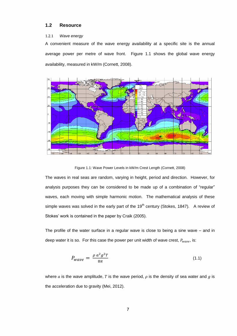
Figure ‎1.3: South Uist Scatter diagram 1976/77 (occurrence in parts per thousand)

(Dawson, 1979)

1.2.2 Wave direction

Much of the available data giving the energy content of the waves, such as that contained

in Figure ‎1.3 does not include wave direction. The Floating Clam being studied here, is

sensitive to wave direction. However even where the WEC itself is not sensitive to wave

direction, the positioning of the individual units within a wave farm will need to be

considered in the light of the prevailing wave direction.

In studying wave direction data it becomes apparent that in many locations the wave

direction although varying, is contained within an arc of up to around 80°, due to the

particular properties of the location such as the prevailing wind and the position of open

sea. Due to the physics of refraction the waves will tend to approach a shallow coast

normally (Mei, 2012). Thus a WEC that is sensitive to wave direction may nevertheless

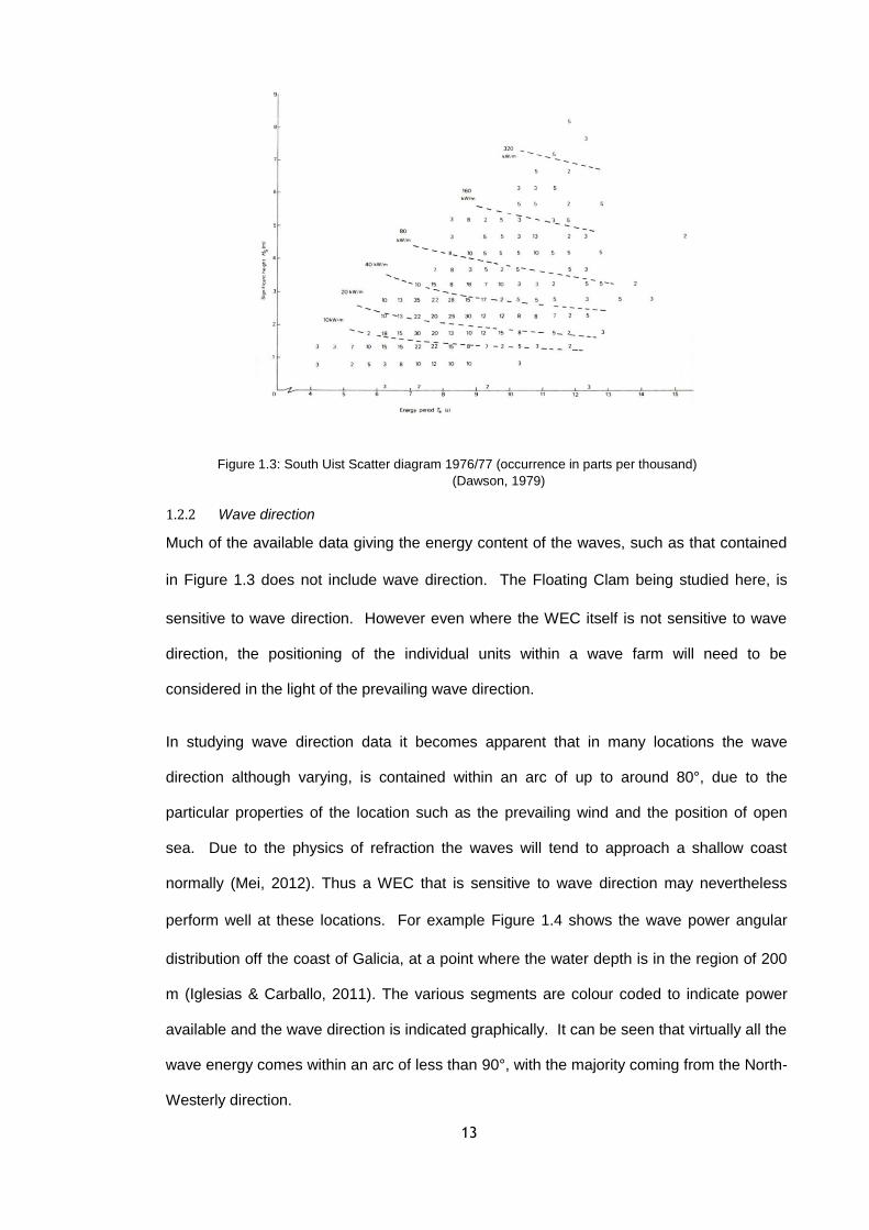
perform well at these locations. For example Figure ‎1.4 shows the wave power angular

distribution off the coast of Galicia, at a point where the water depth is in the region of 200

m (Iglesias & Carballo, 2011). The various segments are colour coded to indicate power

available and the wave direction is indicated graphically. It can be seen that virtually all the

wave energy comes within an arc of less than 90°, with the majority coming from the North-

Westerly direction.

14

Figure ‎1.4: Wave Power Rose at the offshore buoy (Iglesias & Carballo, 2011)

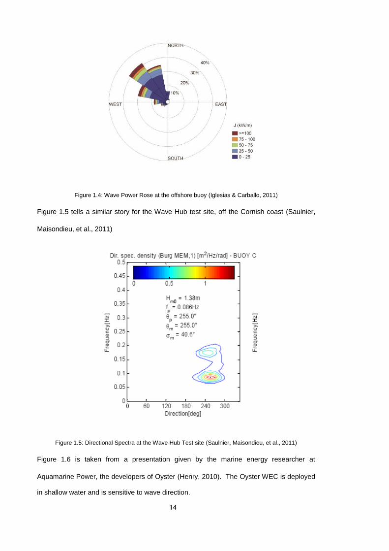
Figure ‎1.5 tells a similar story for the Wave Hub test site, off the Cornish coast (Saulnier,

Maisondieu, et al., 2011)

Figure ‎1.5: Directional Spectra at the Wave Hub Test site (Saulnier, Maisondieu, et al., 2011)

Figure ‎1.6 is taken from a presentation given by the marine energy researcher at

Aquamarine Power, the developers of Oyster (Henry, 2010). The Oyster WEC is deployed

in shallow water and is sensitive to wave direction.

15

Figure ‎1.6: Tightening of directional spectra due to shoaling (Henry, 2010)

During the Oyster development the concept of “wave resource evaluation” or “Exploitable

Wave Power” has been defined as “the net power crossing a line orthogonal to the mean

wave direction” (Henry, 2010).

1.2.3 Length of wave crest and Wave spreading

The mechanisms that govern the ability of the wave energy converter (WEC) to harvest or

“capture” energy are discussed in Section‎1.5.1. However, the theoretical analysis of

energy capture normally starts from the assumption that the wave front is infinitely long and

straight. However, it is clear that this is not the case and that the wave crests will have a

finite length. It is found that short crested waves may be simulated by superimposing plane

waves of differing incident angles, i.e. by a “spread” of wave directions.

One of the most commonly used directional spreading functions is the frequency

dependent cosine power function (Saulnier, Prevosto, et al., 2011), such that:

𝑆(𝑓, 𝜃) = 𝑆(𝑓)𝐷(𝑓, 𝜃) (‎1.15)

where 𝑆(𝑓) is the one-dimensional wave spectrum (or ‘spectral density function’)

𝑆(𝑓, 𝜃) is the directional wave spectrum, and

𝐷(𝑓, 𝜃) is the angular spreading function, given by:

𝐷(𝑓, 𝜃) = C(𝑠)𝑐𝑜𝑠2𝑠 (𝜃

2) (‎1.16)

16

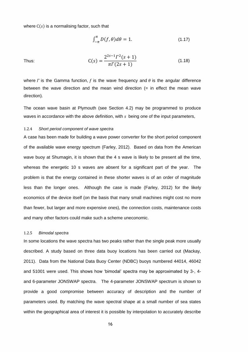
where C(𝑠) is a normalising factor, such that

∫ 𝐷(𝑓, 𝜃)𝑑𝜃𝜋

−𝜋= 1. (‎1.17)

Thus: C(𝑠) =22𝑠−1𝛤2(𝑠 + 1)

𝜋𝛤(2𝑠 + 1) (‎1.18)

where 𝛤 is the Gamma function, 𝑓 is the wave frequency and 𝜃 is the angular difference

between the wave direction and the mean wind direction (= in effect the mean wave

direction).

The ocean wave basin at Plymouth (see Section ‎4.2) may be programmed to produce

waves in accordance with the above definition, with 𝑠 being one of the input parameters,

1.2.4 Short period component of wave spectra

A case has been made for building a wave power converter for the short period component

of the available wave energy spectrum (Farley, 2012). Based on data from the American

wave buoy at Shumagin, it is shown that the 4 s wave is likely to be present all the time,

whereas the energetic 10 s waves are absent for a significant part of the year. The

problem is that the energy contained in these shorter waves is of an order of magnitude

less than the longer ones. Although the case is made (Farley, 2012) for the likely

economics of the device itself (on the basis that many small machines might cost no more

than fewer, but larger and more expensive ones), the connection costs, maintenance costs

and many other factors could make such a scheme uneconomic.

1.2.5 Bimodal spectra

In some locations the wave spectra has two peaks rather than the single peak more usually

described. A study based on three data buoy locations has been carried out (Mackay,

2011). Data from the National Data Buoy Center (NDBC) buoys numbered 44014, 46042

and 51001 were used. This shows how ‘bimodal’ spectra may be approximated by 3-, 4-

and 6-parameter JONSWAP spectra. The 4-parameter JONSWAP spectrum is shown to

provide a good compromise between accuracy of description and the number of

parameters used. By matching the wave spectral shape at a small number of sea states

within the geographical area of interest it is possible by interpolation to accurately describe

17

the wave spectra across the site. This particular study (Mackay, 2011) considers only

omnidirectional spectra and ignores directionality.

1.2.6 Practical resource measurement

Various methods are used to measure ocean waves. The most straightforward method

involves the use of wave measurement buoys that simply float on the top of the wave and

thus provide a measure of the wave position as a function of time. Rather as a cork floats

on water, the lighter and more buoyant the buoy is, the better.

The measurement of a resource such as a potential wave farm site may be estimated from

knowledge of historical wind speeds and their direction – and the local topography. Such

estimates would be compared, for validation purposes, with such wave measurement buoy

data as was available – a process known as ‘hindcasting’.

A more recent development concerns the use of land-based radar for resource

measurement, which has a clear advantage over the use of buoys (Wyatt, 2011).

Estimates may be made of wave power, its directional characteristics and spatial and

temporal variability. Data is obtained (Wyatt, 2011) from two different radars and compared

with buoy data. Data from the Pisces HF radar in the Celtic Sea is used to show evidence

of spatial variations in directionality of the power resource and the results demonstrate that

HF radar can be used to both measure the resource and provide useful monitoring data

during power extraction, device installation, testing and operations. HF wave

measurements are being made at Wave Hub (see next section).

1.2.7 Wave resource at test sites

Spain

The energy resource in the seas off the Galacia coast in NW Spain has been studied, with

the aim of identifying promising areas for the deployment of wave farms (Iglesias &

Carballo, 2011). Measurements from one offshore data collection buoy were taken as the

base data for the study. This data was then split into 104 separately defined wave patterns

or “bins”. Each pattern defined a wave state in terms of significant wave height, energy

period, mean direction and frequency of occurrence. This is essentially the same

18

technique as the “scatter diagram” technique (see Figure ‎1.3), but with the added

parameter of wave direction. The study used the SWAN coastal wave model to compute

the wave resource over a large coastal area for each of 104 combinations of wave height

and period. This enabled the inshore areas of high wave energy resource to be identified

and characterized, the technique being validated by reference to an inshore data collection

buoy. The study showed the potential for this methodology to provide WEC designers with

wave climate data for specific locations.

Cornwall – Wave Hub

Wave Hub Ltd operate the Wave Hub test site where full sized prototype devices may be

tested. Now owned by the Department for Business, Innovation and Skills, the project was

originally developed by the South West of England Regional Development Agency. Up to

four device developers are able to connect their arrays into the Wave Hub, which allows

them to transmit and sell their renewable electricity to the UK's electricity distribution grid.

Each developer is able to locate their devices in one quarter of the 3 by 1 km rectangle

allocated to the Wave Hub, and there is capacity to deliver up to a total of 20 MW of power

into the local distribution network (Wave Hub Ltd, 2016).

A study, aiming to predict the effect of global warming on the wave energy resource at the

Wave Hub test site, has been carried out by Reeve et al. (2011). Tentative conclusions

show that over a 100 year span (comparing 1961-2000 with 2061-2100) wave power will

increase by between 2% and 3%. Of particular interest is the use of the WAVEWATCH III

(WW3) - a third generation wave model developed at NOAA/NCEP in the spirit of the WAM

model (see next paragraph). The model does not require the pre-defined shape of wave

energy spectrum; and since the modelling is capable of generating wave climate data over

the entire computational domain this method can be applied to choosing an optimal site for

a wave farm, in terms of available wave power and/or energy yield.

The WAM model (WAMDI Group, 1988) is commercially available software that provides

predictions of the shape and magnitude of wave spectra based on wind input, water depth

and other location-specific data - avoiding ad-hoc assumptions of spectral shape. It is

19

regarded as superior to earlier models in requiring less empirically derived data, although

some tuning is required for the white-capping dissipation function. The model was

calibrated against fetch-limited wave growth data (WAMDI Group, 1988).

A further study (Saulnier, Maisondieu, et al., 2011) covers the characterisation of the Wave

Hub test site, and shows how the deployment of four buoys in a close array contributes to

the understanding of oceanographic processes, which includes key aspects of uncertainty

and spatio-temporal variability. The local wave energy resource is assessed through time-

domain and frequency-domain analysis, and preliminary results are presented, which have

been obtained from the processing of the extended data, which also includes wind and tidal

information.

Denmark

Estimates have been made of the year-round wave climate at the Danish Wave Energy

Centre (DanWEC) test site at Hanstholm (Margheritini et al., 2011). Use is made of data

from wave measurement buoys and mathematical modelling that computes the wave

climate variation throughout the area of interest. In this case the numerical computation is

carried out by the computer model MILDwave (Universiteit Ghent, 2016).

Ireland

The Sustainable Energy Authority of Ireland is developing the Atlantic Marine Energy Test

Site (AMETS), a grid-connected test area for the deployment of full scale Wave Energy

Converters (WECs) near Belmullet, Co. Mayo, Ireland (Cahill & Lewis, 2011). In common

with the practice employed at other test sites, data is provided by two wave buoys – one

positioned at a deep-water location (100m depth) and the other further inshore (50m

depth), in order to characterise the wave resource at the site. There is no attempt at

modelling the spatial variability of the resource, but comparison of the measurements from

the two wave buoys indicates a considerable level of homogeneity over the site. The

resource at the quarter scale site at Galway Bay is compared with the resource at AMETS

and the degree of scalability between the two sites is assessed. Also, estimates of annual

energy capture of the Pelamis WEC are presented.

20

1.3 Hydrodynamic analysis

The behaviour of an incompressible fluid may be described by the Navier-Stokes

equations. These equations govern the motion of a viscous fluid subject only to the

assumptions of constant density and a Newtonian stress-strain relationship (Newman,

1977). The Navier-Stokes equations, written in full and in Cartesian coordinates are:

𝜕𝑢

𝜕𝑡+ u

𝜕𝑢

𝜕𝑥+ v

𝜕𝑢

𝜕𝑦+ w

𝜕𝑢

𝜕𝑧= −

1

𝜌

𝜕𝑝

𝜕𝑥+

𝜇

𝜌∇2𝑢 +

1

𝜌𝐹𝑥

𝜕𝑣

𝜕𝑡+ u

𝜕𝑣

𝜕𝑥+ v

𝜕𝑣

𝜕𝑦+ w

𝜕𝑣

𝜕𝑧= −

1

𝜌

𝜕𝑝

𝜕𝑦+

𝜇

𝜌∇2𝑣 +

1

𝜌𝐹𝑦

𝜕𝑤

𝜕𝑡+ u

𝜕𝑤

𝜕𝑥+ v

𝜕𝑤

𝜕𝑦+ w

𝜕𝑤

𝜕𝑧= −

1

𝜌

𝜕𝑝

𝜕𝑥+

𝜇

𝜌∇2𝑤 +

1

𝜌𝐹𝑧

(‎1.19)

where 𝑥, 𝑦, and 𝑧 are the Cartesian coordinates of a point in the fluid and 𝑢, 𝑣, and 𝑤 are the

corresponding velocities of the fluid. Fluid density is 𝜌, viscosity is 𝜇 and 𝑡 is time. 𝐹𝑥 , 𝐹𝑦, 𝐹𝑧

are the external forces acting the fluid.

The Continuity Equation is also required:

𝜕𝑢

𝜕𝑥+

𝜕𝑣

𝜕𝑦+

𝜕𝑤

𝜕𝑧= 0 (‎1.20)

The Navier-Stokes equations are difficult to solve as they form a coupled system of

nonlinear partial differential equations which may be solved analytically only for some very

simple geometrical configurations. However, by making the assumption of an inviscid fluid

the equations become much simpler and easier to solve. This results in the discovery that

the velocity field may be represented by the gradient of a scalar function, the Velocity

Potential, 𝜑. The fluid is said to be “irrotational” (Newman, 1977).

In the case of large objects, such as ships and wave energy converters (WEC) the effect of

fluid viscosity on the overall flow pattern is slight. The viscous forces in the main body of

fluid are small, so that in these areas the assumption of an inviscid, irrotational fluid

becomes valid (Newman, 1977). The effect of viscous forces, such as skin friction may

then be included in the analysis as additional terms in the equations of motion etc.

21

Historically this approach has proved successful but with the advent of powerful computers

more advanced methods that solve the complete Navier Stokes equation are being used.

Recent research carried out at the University of Plymouth has demonstrated the use of

such methods to assess the survivability of a WEC in severe waves (Ransley, 2015).

With the assumption of zero viscosity it can be shown that the velocity profiles within the

fluid satisfy the Laplace Equation (Equation‎1.21), and, as in the case of the Clam, a good

understanding of the dynamics of the WEC may be gained through this simplification.

𝜕2𝜑

𝜕𝑥2+

𝜕2𝜑

𝜕𝑦2+

𝜕2𝜑

𝜕𝑧2= 0 (‎1.21)

where 𝜑 is the Velocity Potential and 𝑥, 𝑦 and 𝑧 are the Cartesian coordinates.

The important conclusion to be drawn from this relationship is that the fluid motion depends

only on the velocity of the fluid at its boundaries and may be completely described by the

fluid velocity normal to the surface – and the geometry of the surface.

In the case of a stationary surface the fluid velocity normal to the surface is zero – although

the flow may be along the surface. However, in the case of a free surface, such as a sea

wave, the velocity of the boundary is unknown. In this case, knowledge of the pressure on

the free surface leads to a solution using Bernoulli’s equation (Newman, 1977, Section 4.3).

An introduction to the theory of water waves, using basic level calculus, is provided by the

book, “Water Waves” (Barber & Ghey, 1969), which has the merit of helping the reader

understand the fundamental concepts, including the derivation of the Laplace Equation

without the need of advanced mathematics. More recent textbooks, such as “Water Wave

Mechanics for Engineers and Scientists” (Dean & Dalrymple, 1991) cover the derivation of

the Laplace Equation and the solution of hydrodynamic problems through more advance

techniques including vector analysis.

22

1.4 Analysis tools

1.4.1 AQWA and WAMIT

Two commercially available numerical analysis tools have been investigated here for

application to the Clam: WAMIT (WAMIT, 2012) and AQWA (Ansys, 2010). Both analyse

the hydrodynamics of fixed and floating bodies, and wave makers, based on the use of the

Velocity Potential, 𝜑, as described in the previous section. Both use the boundary-value

method to compute the results for points on a user-specified mesh. Virtually identical

results are obtained from these tools in terms of the basic analysis, using the same mesh

geometry. However their development has followed different paths.

WAMIT consists, in effect, of a toolbox of analysis methods of varying degrees of

sophistication, including the very useful ability to “patch in” sections of the surface from a

menu of geometric shapes. Additionally there is the technique of using “generalised modes”

that facilitates the analysis of a range of problems; particularly those involving flexible

bodies, where the body flexure affects the hydrodynamic behaviour of the system. The

WAMIT package itself has no graphics capability, but may be used in conjunction with a

graphics package – MultiSurf (AeroHydro, 2012).

All versions of WAMIT earlier than version 6 were based strictly on the low-order panel

method, where the geometric form of the submerged body surface is defined by flat

quadrilateral elements and the solutions for the velocity potential and/or source strength are

assumed constant on each panel. WAMIT Version 6 has been extended to include a

complementary higher-order panel method based on a continuous B-spline representation

for the velocity potential, and several alternative schemes for defining the body surface

including explicit analytic formulae. The order of the B-splines is controlled by user-

specified input parameters.

AQWA on the other hand is less sophisticated in regard to the mathematical methods on

which it is based, being equivalent to the “low order” WAMIT methodology. Meshing is

based on two simple shapes, the plane triangle and quadrilateral, and curved surfaces are

modelled by refining the mesh. Although WAMIT has an advanced capability that can

23

model curvature accurately, AQWA has a sophisticated graphical front end, the Ansys

Workbench, which enables the user to visually build the model. AQWA also uses non-

diffracting surface that allow visualisation of the parts of the model above the water surface.

The term “non-diffracting” is used (by AQWA) to describe elements that are not part of the

hydrodynamic calculations. Also much use is made of “Morison elements” that allow

hydrodynamically small objects to be included, such as mooring lines.

Morison’s Formula (Newman, 1977) assumes that the total wave force is the sum of inertia

forces and viscous forces, i.e.:

𝐹𝑜𝑟𝑐𝑒 = (𝑎𝑑𝑑𝑒𝑑 𝑚𝑎𝑠𝑠 + 𝑏𝑜𝑑𝑦 𝑚𝑎𝑠𝑠) × 𝑎𝑐𝑐𝑒𝑙𝑒𝑟𝑎𝑡𝑖𝑜𝑛 + 𝑣𝑖𝑠𝑐𝑜𝑢𝑠𝑓𝑜𝑟𝑐𝑒𝑠 (‎1.22)

Viscous forces usually take the form, 1

2𝜌𝐴𝐶𝐷𝑈|𝑈| , where 𝜌 is the water density, 𝐴 , is

representative area, 𝑈 is the body velocity relative to the fluid, and 𝐶𝐷 is an appropriate

drag coefficient.

It should be noted that Morison’s Formula is semi-empirical and depends on the use of

factors based on model tests and takes no account of the force on the body due to radiated

waves. In AQWA it is only used on tubular elements, and is particularly useful in modelling

mooring lines, and in adding viscous drag to a moving object or one subjected to currents.

In addition, through a mathematical technique that uses the Convolution Integral, AQWA

turns a frequency domain solution into a time domain simulation that can be displayed as

an animation.

Because AQWA is a commercial package designed to support the shipping and off-shore

industry it contains the ability to model a moving object. It is able to model slow-drift and

extreme wave conditions and enables the user to study transient effects such as line

breakage (through the use of “Convolution”).

Although neither package, WAMIT or AQWA, is as straightforward as could be wished,

WAMIT is the application that best fits the needs of the current programme, since the

method of “generalised modes” is ideally suited to modelling the Clam action.

24

WAMIT’s use of text files allows easy interface with other PC applications. However the

absence of a built-in graphical interface, such as provided by AQWA means that it is not as

easy to detect errors. Successful use depends on the skill and diligence of the user.

1.4.2 Excel spreadsheet

MS EXCEL is particularly useful in analysing data from wave tank trials. All the files

generated during the wave tank testing are text files. This means that the files can be

readily input into the EXCEL spreadsheets.

1.4.3 Mathcad

Mathcad (PTC, 2014) has been used for this project. It provides a similar capability to

other mathematical analysis packages such as MATLAB (Mathworks, 2014) and Maple

(Maplesoft, 2014).

1.4.4 Time domain model

VisSim (Visual Solutions, 2014) has been used in this project for time domain modelling. It

provides a similar capability to MATLAB/Simulink (Mathworks, 2014), but is easy to use

and fast. The Clam has been modelled in the time domain using a regular wave input and

perfect agreement with the frequency domain models has been achieved. The simulation

has also been extended to provide a time domain model employing a random input and

taking account of the various non-linear elements (e.g. drag and Coulomb friction). VisSim

is also capable of being modified to incorporate the mathematically correct “convolution

integral” approach.

25

1.5 Power capture and control

1.5.1 Mechanism of power capture

Power Capture is, as the name implies, the power harvested by the Wave Energy

Converter (WEC) and is clearly dependent on the power in the sea state of interest. As

discussed in Section ‎1.2.1 the wave power per unit width of wave front, 𝑃𝑤𝑎𝑣𝑒, may be

computed from Equation ‎1.9, given the significant wave height, 𝐻𝑠, and energy period, 𝑇𝑒.

A measure that can be used to compare WECs is the Capture Width, 𝑊𝐶, which is found by

dividing the Power Capture, 𝑃, by the power in the incoming wave:

Thus: 𝑊𝑐 =𝑃

𝑃𝑤𝑎𝑣𝑒 . (‎1.23)

Power capture clearly depends on the response of the Wave Energy Converter (WEC) to

incoming waves. Most WECs absorb energy from the sea by resonating with periods at, or

close to that of the sea waves. This mode of power capture relies on the WEC being a

good wave maker. As Falnes (2002) explains, energy is taken from the wave by a process

that involves cancelling the wave action as it passes the wave energy converter (WEC).

When maximum energy is absorbed the sea behind the converter is perfectly calm and all

the energy in the incoming wave is absorbed. Since the system may be considered (as a

good approximation) to be linear, the pattern of waves is the sum of the unaffected

incoming wave plus the wave system generated by the WEC.

The greatest transfer of energy occurs when the motion of the WEC has a particular phase

and amplitude relation with the incoming wave. Referring to Figure ‎1.7, it can be seen that

the amplitudes of the radiated wave (curves b and c) have to be half the amplitude of the

incoming wave (curve a). Additionally, the radiated wave has to have the right phase

relationship with the incoming wave, such that the crests of the wave radiating towards the

right (curves b and c) coincide with the troughs of the incident wave (curve a).

Figure ‎1.7d shows an ideal case where all the wave energy is absorbed. However, where

there is only one mode of oscillation (e.g. a heaving absorber) the resulting wave

26

corresponds to the superposition of waves a and b. Note that the wave radiated towards

the left and the resulting wave transmitted towards the right both have an amplitude equal

to half of the amplitude of the incident wave. Since wave energy is proportional to the

square of the wave amplitude this means that 25% of the incident wave energy is reflected

towards the left, and also 25% of it is transmitted towards the right. The remaining 50% is

absorbed by the WEC, the theoretical maximum.

Figure ‎1.7: Modes of energy absorption (Falnes, 2002)

1.5.2 Resonance

The optimal phase condition for the WEC is when it is in resonance with the waves (Falnes,

2005). Thus its natural resonant period should be the same as the wave period. In a

practical device it is difficult to maintain this relationship as the wave period changes with

sea state, and also to some extent, from one wave to the next. A measure of the ability of

the device to pick up energy when operating away from maximum resonance is its

bandwidth. It is found that physically large WECs have broad bandwidths, such as

SPERBOYTM

(Phillips & Rainey, 2005). However, the drawback of a large WEC lies in the

cost of materials, length of construction time and increased difficulties of deployment.

A smaller WEC will have a narrower bandwidth. But in this case the energy transfer may

be improved in two ways: firstly by actively changing the resonant period (i.e. by “tuning”),

and secondly by applying some form of phase control in order to obtain the optimum phase

condition. A method that has been well researched is to achieve phase control by latching.

However, before looking at latching, the performance of point absorbers is discussed.

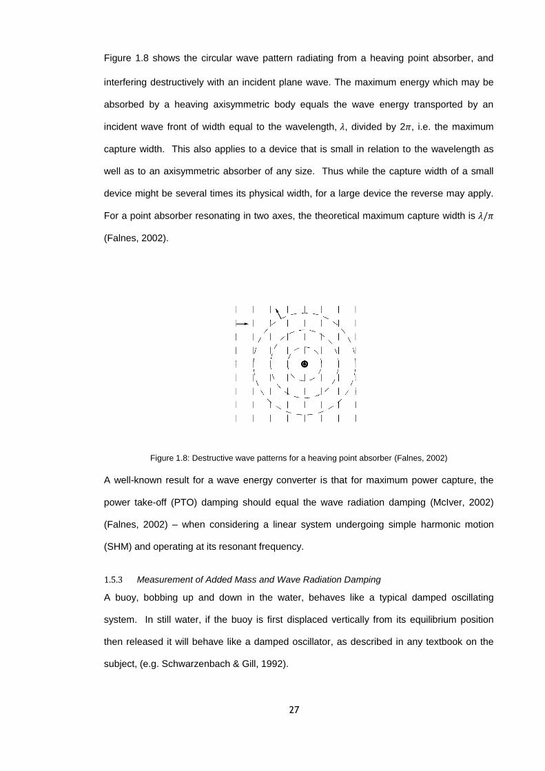
27

Figure ‎1.8 shows the circular wave pattern radiating from a heaving point absorber, and

interfering destructively with an incident plane wave. The maximum energy which may be

absorbed by a heaving axisymmetric body equals the wave energy transported by an

incident wave front of width equal to the wavelength, 𝜆, divided by 2𝜋, i.e. the maximum

capture width. This also applies to a device that is small in relation to the wavelength as

well as to an axisymmetric absorber of any size. Thus while the capture width of a small

device might be several times its physical width, for a large device the reverse may apply.

For a point absorber resonating in two axes, the theoretical maximum capture width is 𝜆/𝜋

(Falnes, 2002).

Figure ‎1.8: Destructive wave patterns for a heaving point absorber (Falnes, 2002)

A well-known result for a wave energy converter is that for maximum power capture, the

power take-off (PTO) damping should equal the wave radiation damping (McIver, 2002)

(Falnes, 2002) – when considering a linear system undergoing simple harmonic motion

(SHM) and operating at its resonant frequency.

1.5.3 Measurement of Added Mass and Wave Radiation Damping

A buoy, bobbing up and down in the water, behaves like a typical damped oscillating

system. In still water, if the buoy is first displaced vertically from its equilibrium position

then released it will behave like a damped oscillator, as described in any textbook on the

subject, (e.g. Schwarzenbach & Gill, 1992).

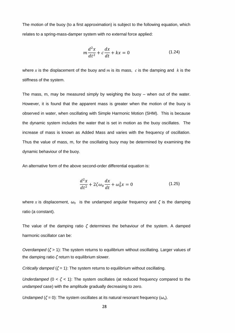
28

The motion of the buoy (to a first approximation) is subject to the following equation, which

relates to a spring-mass-damper system with no external force applied:

𝑚𝑑2𝑥

𝑑𝑡2+ 𝑐

𝑑𝑥

𝑑𝑡+ 𝑘𝑥 = 0 (‎1.24)

where 𝑥 is the displacement of the buoy and 𝑚 is its mass, 𝑐 is the damping and 𝑘 is the

stiffness of the system.

The mass, m, may be measured simply by weighing the buoy – when out of the water.

However, it is found that the apparent mass is greater when the motion of the buoy is

observed in water, when oscillating with Simple Harmonic Motion (SHM). This is because

the dynamic system includes the water that is set in motion as the buoy oscillates. The

increase of mass is known as Added Mass and varies with the frequency of oscillation.

Thus the value of mass, m, for the oscillating buoy may be determined by examining the

dynamic behaviour of the buoy.

An alternative form of the above second-order differential equation is:

𝑑2𝑥

𝑑𝑡2+ 2𝜁𝜔0

𝑑𝑥

𝑑𝑡+ 𝜔0

2𝑥 = 0 (‎1.25)

where 𝑥 is displacement, ω0 is the undamped angular frequency and ζ is the damping

ratio (a constant).

The value of the damping ratio ζ determines the behaviour of the system. A damped

harmonic oscillator can be:

Overdamped (ζ > 1): The system returns to equilibrium without oscillating. Larger values of

the damping ratio ζ return to equilibrium slower.

Critically damped (ζ = 1): The system returns to equilibrium without oscillating.

Underdamped (0 < ζ < 1): The system oscillates (at reduced frequency compared to the

undamped case) with the amplitude gradually decreasing to zero.

Undamped (ζ = 0): The system oscillates at its natural resonant frequency (ωo).

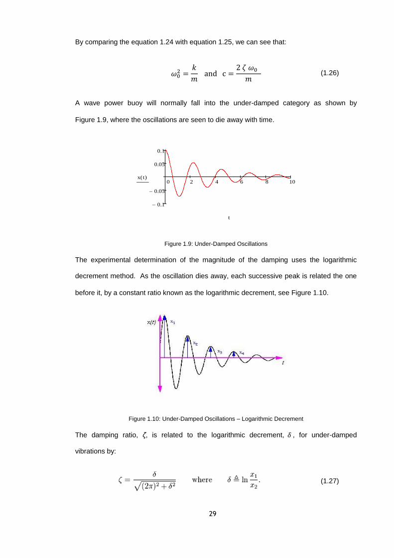
29

By comparing the equation ‎1.24 with equation ‎1.25, we can see that:

𝜔02 =

𝑘

𝑚 and c =

2 𝜁 𝜔0

𝑚 (‎1.26)

A wave power buoy will normally fall into the under-damped category as shown by

Figure ‎1.9, where the oscillations are seen to die away with time.

Figure ‎1.9: Under-Damped Oscillations

The experimental determination of the magnitude of the damping uses the logarithmic

decrement method. As the oscillation dies away, each successive peak is related the one

before it, by a constant ratio known as the logarithmic decrement, see Figure ‎1.10.

Figure ‎1.10: Under-Damped Oscillations – Logarithmic Decrement

The damping ratio, ζ, is related to the logarithmic decrement, 𝛿 , for under-damped

vibrations by:

(‎1.27)

0 2 4 6 8 10

0.1-

0.05-

0.05

0.1

x t( )

t

30

1.5.4 Reactive control

“Optimum” or “reactive” control seeks to maximise the energy capture by returning some

energy to the sea during part of the oscillatory cycle and re-capturing it during a later part of

the cycle. To optimally apply this strategy it is necessary to measure the waves and/or the

WEC’s oscillatory motion, and thus predict the wave pattern some seconds into the future.

A similar strategy is “latching phase control” - see Figure ‎1.11. This is employed where the

wave periods are longer than the WEC’s natural period. A Clamping mechanism stops the

motion at the instant of extreme excursion. Further motion is then permitted after a certain

time (about one quarter of the natural period) before the next maximum of the wave

exciting force. For a heaving buoy of natural period shorter than the wave period this force

is approximately in phase with the wave elevation of the incident wave (Falnes, 2002).

Figure ‎1.11: Resonance and phase control (Falnes, 2005)

Referring to Figure ‎1.11, the curves indicate incident wave elevation and vertical

displacement of a heaving body as functions of time.

Curve a shows the elevation of the water surface due to the incident wave. This would also

represent the vertical position of a body with negligible mass. For a body of diameter very

small compared to the wavelength, curve a also represents the wave’s heave exciting force

on the body.

31

Curve b shows the vertical displacement of heaving body whose mass is such that its

natural period is equal to the wave period (resonance).

Curve c shows the vertical displacement of a body with smaller mass, and hence shorter

natural period, which would normally not keep in phase with the incoming wave. Phase

control is then obtained by keeping the body in a fixed vertical position for a certain time.

Figure ‎1.12 show the results of a simulation study (Falnes, 2005). The curves show the

wave energy (in joules) accumulated during 5 seconds for three cases, i.e. no control

(lower broken curve), latching phase control (solid curve) and full, theoretically ideal

optimum control (broken wavy curve). The practical limitation of amplitude is ignored, For

the last case it is seen that relatively large amounts of energy have to be returned to the

sea during two intervals of each oscillation cycle. The result is that the energy absorbed is

about twice the absorbed energy under latching phase control, and this latter energy is

about four times as much as that without any control (Falnes, 2005).

Figure ‎1.12: Phase and Latching Control – a comparison (Falnes, 2005)

For real sea waves the time intervals between crests and troughs vary in a random

manner. With operation of a latching-controlled WEC in such random waves the point of

release is determined by a control system that uses signals from sensors measuring the

wave position or the wave exciting force in order to make a prediction of the wave force at a

future time. The decision to unlatch the WEC should be taken at least one quarter of the

WEC’s natural period before the next extreme of the wave force (Falnes, 2005).

32

1.5.5 Power Take-Off (PTO) and associated control systems

The possible technical solutions for the PTO and its control systems clearly depend on the

type of WEC under consideration. In reviewing the literature it appears that among the

multiplicity of concepts, there is more commonality in control methodology than in

hardware.

The least efficient, but possibly the easiest control methodology to implement, is the type of

control based on resonance (see Section ‎1.5.2) and which can be described as impedance

matching. This is almost the only option available to oscillating water column (OWC)

devices, where the movement of the water column pumps air through a turbine/generator

set. A practical solution is to match the characteristics of the turbine and the resonant

period of oscillation of the WEC to the wave resource, as has been proposed for the

SPERBOYTM

WEC (Phillips & Rainey, 2005). A certain degree of reactive control may be

possible, dependent on the characteristics of the turbine, and this has been the object of

recent research at Plymouth (Freeman, 2011). It is seen that the most appropriate control

system will be dependent on the type of WEC and its PTO. Practical considerations such

as the stall characteristics of an air turbine and the behaviour of the WEC in heavy seas

influence the choice of control system. Reactive control where power is input to the WEC

during part of the wave cycle provides greater overall power capture than simple

impedance matching (Freeman, 2011). Normally the turbine is designed to rotate in the

same direction irrespective of the direction of air flow, which reciprocates. Suitable turbine

types include the Wells turbine and the impulse turbine. Among the WEC design options

are those where the WEC is incorporated into a fixed structure such as a breakwater. Here

it is possible to maximise power capture by for example controlling the speed of the turbine

and by controlling the resonance of the system. Where the turbine communicates with a

closed air chamber, the resonant period may be altered by actively modifying its pressure

and/or volume, as proposed for a breakwater to be installed off the Italian La Spezia coast.

(Filianoti, P & Camporeale, S M, 2005). A similar scheme is to be installed in a caisson

forming the head of the new Douro breakwater near Porto, Portugal. The PTO comprises a

33

Wells turbine and a variable speed generator whose optimum speed is computed for each

sea state. (Gato et al., 2005).

PTO systems based on the use of hydraulic machinery are proposed by many developers.

These commonly include hydraulic rams, hydraulic motors and accumulators. One such

application is shown in Figure ‎1.13. This particular system has been modelled by using

hydrodynamic coefficients based on linear theory within a non-linear time domain analysis.

A simplified one-dimensional (heave) model has been developed to include the convolution

integral approach (Falcão, 2005). The PTO and the same modelling approach may be

developed to include phase control by latching (Falcão, 2007).

Figure ‎1.13: Heaving Point Absorber with Hydraulic PTO (Falcão, 2005)

Studies of a heaving point absorber WEC equipped with hydraulic energy storage and a

variable speed generator Doubly-Fed Induction Generator (DFIG) have been carried out

with the aid of a generic wave-to-wire dynamic model. The emphasis was on developing a

control strategy for the intermediate (hydraulic) energy stage and the generator (Kiprakis &

Wallace, 2005). The electrical engineering aspects were fully examined but the control

philosophy appears little more advanced than that of impedance and resonance matching.

34

A theoretical framework has been devised to analyse the behaviour and energy collection

potential of a wave energy converter operating in random waves under latching control.

Applying the analysis to a heaving buoy demonstrates the effectiveness of latching, and the

method is readily applicable to other types of WEC (Babarit & Clément, 2005).

Control methods and performance figures for a heaving point absorber have been

investigated where the WEC takes the form of a semi-submerged sphere. This has

demonstrated the significant increase of absorbed wave power due to phase control. The

difference between optimum reactive control and sub-optimum latching control was less

significant. Unfortunately the experimental work was flawed by excessive friction levels in

the test set-up (Torkel & Falnes, 2005).

MacTaggart Scott have developed an infinitely variable reactive control system that offers

increased energy capture for wave power devices that use a hydraulic PTO. This they call

a “Reactive Hydraulic Modulator (RHM)”. MacTaggart Scott are considering the use of

seawater as the working medium. Also claimed is that active control may be used to

smooth wave farm output and ‘detune’ the device, thus allowing continued generation in

higher sea states (Skinner & Scott, 2010).

Not all devices employ a PTO control system that falls into one of the above categories. A

case in point is the Oyster WEC, which is an Oscillating wave surge converter (OWSC),

where the enhanced horizontal fluid particle movement of waves in the near shore coastal

zone is exploited (Whittaker & Folley, 2012). Oyster does not follow the conventional

wisdom of Section ‎1.5.2, it “couples with incoming waves without being highly tuned” and

aims to optimise the wave torque (Whittaker et al., 2007).

A further PTO system concept is the use of a compact array of small buoys that are not

resonated. The theoretical potential of the compact array have been compared with that of

a large buoy of equal volume, and shown to be superior (Mei, 2012).

35

1.6 Sea keeping

By their very nature, wave energy devices need to be sited in areas of high wave energy,

and thus a floating WEC will need to be sufficiently stable in rough seas. Normal, well

established criteria may be used to calculate such parameters as the centre of gravity,

centre of buoyancy and metacentric height (Francis, 1962). The natural periods of pitch

and roll should also be predicted. If these are not relevant to the energy capture, then the

periods should be of the order of 30 seconds – long enough to avoid resonance in storm

conditions but short enough to give a satisfactory level of static stability.

In this connection it is necessary to consider how the sea-keeping ability of the device

affects its maintainability – methods of altering its response when undergoing maintenance

may have to be considered. It should be noted that as well as calculating the

hydrodynamic characteristics of a floating body, AQWA also computes its static stability.

Wave tank testing, incorporating correctly scaled models is essential to assess the

behaviour of a device in storm conditions, since the assumption of linearity breaks down in

this case. In addition, wave tank testing may show up aspects that have not been

previously considered.

1.7 Wave energy converters – a comparison

As explained in Section ‎1.1, wave energy research in the UK was actively pursued in the

1970s although there was a decision to cease funding in favour of the nuclear industry in

the 1980s. However, due to threat of global warming and the need to find renewable

energy sources, wave energy is again receiving government attention and support.

There are now well over 170 individual devices that have been proposed to extract energy

from sea waves (Joubert et al., 2013). Many of these have been patented and tested in an

ad hoc fashion. Some have been built, tested and subjected to scientific scrutiny, but as yet

there are no clear winners since the viability of a WEC depends on its energy collection

efficiency measured in pence per kW-hour (or similar) having taken all factors into

consideration, i.e. cost of construction, energy capture performance, maintenance, etc.

36

There are a number of fundamentally different ways of extracting energy from the sea

(Phillips, 2008), the main ones being listed below. Examples of each type are given,

although many more could be quoted.

Articulated pontoons – Cockerell Raft, McCabe Wave Pump, Pelamis

Here the PTO utilises the rotary motion of, and torque applied to the

hinges that join the floating pontoons. The McCabe Wave Pump is

designed to produce high pressure water for desalination. The Pelamis’

hinges take the form of hydraulic rams that allow movement in any

direction.

Oscillating Water Column (OWC) – Limpet, SPERBOYTM

Typically OWCs embody a duct whose lower end is below the sea surface.

The duct then continues to a level above the surface where it feeds into a

turbo-generator set. The wave action causes air to be pumped through the

turbine. OWCs may be shore mounted as in the case of Limpet or

incorporated into a floating structure such as SPERBOYTM

.

Heaving Buoy – AquaBuoy, SPERBOYTM

, Ocean Power Technologies (OPT)

As the name implies, a heaving buoy rises and falls with the wave

action. They usually have an axisymmetric structure and are classed as

point absorbers. The range of possible PTOs is wide. AquaBuoy, although

not now being developed, was tethered directly to the ocean floor via an

ingenious “hose pump” that pumped water as it was alternately stretched

and relaxed. The OPT device incorporates a reaction plate placed below

the buoy and is thus in relatively still water.

Over-topping – Wave Dragon

Wave action causes water to flow up a ramp and over the edge where it is

collected and used to drive low-head turbine/generator sets. Wave Dragon

incorporates arms that gather waves from an area much wider than the

entry to the ramp.

Float-operated – Wave Star, Manchester Bobber

Float operated devices are usually based on the principle of a hinged arm

with a float at its extremity, e.g. Wave Star which uses a multiplicity of

such floats. The Manchester Bobber embodies floats arranged in a matrix

pattern each float being suspended by cable in such a way as to drive a

drum forming part of the PTO mechanism.

Hinged paddle – Oyster

Deployed close to shore, the Oyster consist of one large flap hinged at the

37

sea bed, such that wave action causes it to oscillate back and forth. Power

is absorbed via hydraulic rams attached to the flap.

Others – PS Frog, Salter’s Duck, Bristol Cylinder, Anaconda

PS Frog – a buoyant paddle with a ballasted mass within it.

Salter’s Duck – a buoyant duck-shaped body that oscillates around a spine.

The PTO may take a number of forms including by internal gyroscopic

action. Hydrodynamically very efficient.

Bristol Cylinder – a cylindrically shaped and buoyant body tethered below

the sea surface. The tethers are connected to subsea PTO units.

Anaconda – a submerged rubber tube that carries a bulge wave as the

wave passed along it.

In most cases the performance of the WEC depends on resonance. However this is not

true for the overtopping device, and has limited applicability to the hinged paddle. In

addition, Mei (2012) demonstrates mathematically that a large, compact array of buoys

(e.g. the Manchester Bobber) has a wide band response that does not rely on resonance

for energy extraction.

There are many reasons why the most efficient device, in terms of energy extraction, may

not provide the most economical solution as measured by p/kWh taken over its full life.

Often the actual performance is less than that predicted by analyses that assume an ideal,

frictionless fluid – and it is these optimistic predictions that are given by WAMIT or AQWA.

The cost of maintenance is also a major factor. Thus a simple and robust device could

prove to be a better solution than a more efficient, but more complicated one. Hinged

devices may seem simple, but the loads on the associated mechanisms can be very high

and bearing failure is a potential problem – the articulated pontoon falls into this category.

Oyster avoids the problem to a great extent by allowing the paddle to move freely in storm

conditions. It is believed that this is not an option for Pelamis and that active control is

needed to prevent structural failure. Bearing failure has been a problem for Pelamis –

although now overcome.

A more recent development is the approach taken by AWS (AWS, 2012) who, after two

unsuccessful development projects, AWS-I and AWS-II, chose to resurrect a concept

pioneered in the 1980s by the Energy Systems Group, of Coventry’s Lanchester

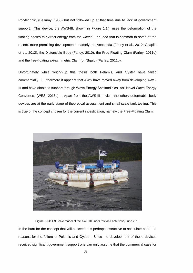
38

Polytechnic, (Bellamy, 1985) but not followed up at that time due to lack of government

support. This device, the AWS-III, shown in Figure ‎1.14, uses the deformation of the

floating bodies to extract energy from the waves – an idea that is common to some of the

recent, more promising developments, namely the Anaconda (Farley et al., 2012; Chaplin

et al., 2012), the Distensible Buoy (Farley, 2010), the Free-Floating Clam (Farley, 2011d)

and the free-floating axi-symmetric Clam (or “Squid) (Farley, 2011b).

Unfortunately while writing-up this thesis both Pelamis, and Oyster have failed

commercially. Furthermore it appears that AWS have moved away from developing AWS-

III and have obtained support through Wave Energy Scotland’s call for Novel Wave Energy

Converters (WES, 2016a). Apart from the AWS-III device, the other, deformable body

devices are at the early stage of theoretical assessment and small-scale tank testing. This

is true of the concept chosen for the current investigation, namely the Free-Floating Clam.

Figure ‎1.14: 1:9 Scale model of the AWS-III under test on Loch Ness, June 2010

In the hunt for the concept that will succeed it is perhaps instructive to speculate as to the

reasons for the failure of Pelamis and Oyster. Since the development of these devices

received significant government support one can only assume that the commercial case for

39

both of them was not sufficiently attractive to a private investor, i.e. a large public company

and possibly also to an energy supplier who would require a system that would provide

electrical power at a sufficiently low cost. Pelamis would appear to be too complicated, and

full of expensive hydraulic machinery that would be subject to large oscillating loads.

Oyster seemed to be a good workman-like device, but with two failings. Firstly, dependent

on the nature of the sea bed its attachment could be difficult, particularly as it needs to

resist continuously oscillating loads. Secondly, in comparison with moored devices the

possible deployment locations are limited since it must be installed in sufficiently shallow

water. Potential sites could be limited since if close to the shoreline, it would provide a

potentially significant hazard to small boats, swimmers, etc.

The conclusion is then that the ultimate prize will go to the developers of a WEC that is not

only efficient in terms of harvesting wave power in the hydrodynamic sense, but also

employs a simple and robust PTO. It should also be capable of adaption to a wide range of

locations.

40

2 Device Development and Physical

Modelling

2.1 Introduction

During the course of the study several physical models have been trialled. The purpose of

this section of the report is to describe these physical models and their construction,

together with the reasons for the various changes. Details of the trials and their analysis

are dealt with in Chapter ‎4 while the development of the mathematical models is covered in

Chapter ‎3.

However, before looking the physical models it is useful to consider how the present study

would fit into the overall development of a wave energy converter – through to full scale

deployment.

2.2 Development pathway

In bringing a new device to the point of full scale commercial deployment it is clear that the

project needs to progress in a logical manner. Hence it is desirable that the development

moves forward in phases, where progress to each phase depends on the satisfactory

outcome of the previous phase. The Hydraulic & Maritime Research Centre (HMRC) have

put forward a protocol for the development of wave energy converters (WECs) that has

been generally accepted by the industry (Holmes et al., 2007). The five phases are:

1. Validation Model - Fundamental Testing in Regular & Random Waves

2. Design Model - Testing in Realistic Sea Conditions

3. Process Model - Testing in Conditions Representative of Deployment Site

4. Prototype Model - Large Scale Pilot Plant at Sea

5. Demonstration Model - Pre-production prototype

The process is very much orientated around the model scale. Phases 1 and 2 typically

employ models of say 1:25 or 1:50. The phase 3 model would be 1:6 or 1:10 and phase 4

and 5 employ full scale devices. The mathematical modelling becomes more detailed as

the project proceeds.

41

What appears to be missing in the HMRC description of the process is an important activity

– that of preparing a feasibility study and updating it as the project progresses. This is a

vital task in ensuring the success of a commercial venture by identifying the best way

forward and the development paths to avoid. The process of preparing a feasibility study is

a well-documented activity where all aspects of the venture are considered.

Before even embarking on a programme such as the HMRC protocol it is clearly a good

idea to establish whether a particular device has potential – at least as a concept – and this

is where the present study fits in. During the course of study the Clam’s energy capture

performance has been assessed. Practical testing, that is at a level broadly consistent with

HMRC’s phase1 activity has been carried out and a parallel theoretical study has been

undertaken. The study concludes by describing the main features of a design for a full size

WEC moored at the Wave Hub test site and predicts its annual energy capture (see

Chapter ‎5).

Future development of the Clam (outside the scope of the present study) would follow the

HMRC protocol from stage 1 – supported by a comprehensive feasibility study.

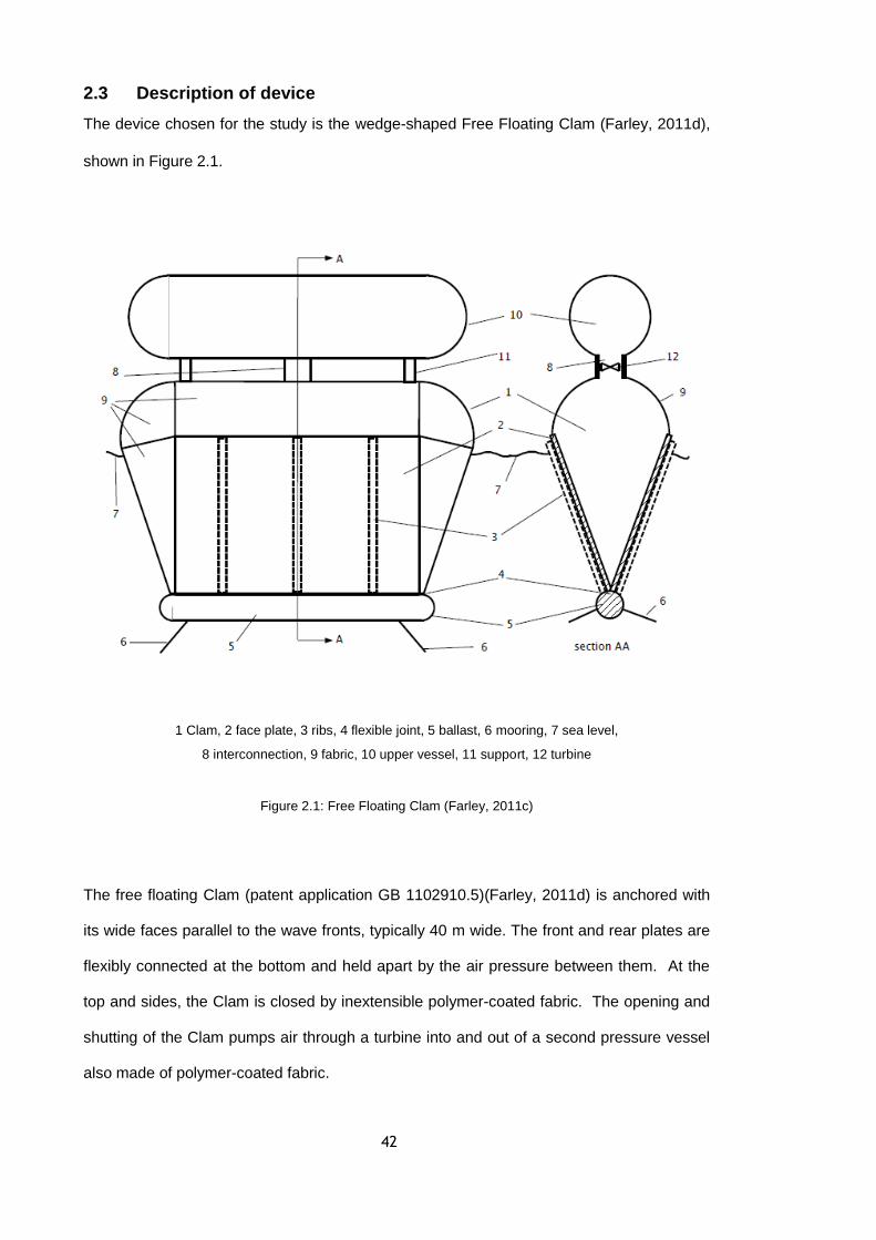
42

2.3 Description of device

The device chosen for the study is the wedge-shaped Free Floating Clam (Farley, 2011d),

shown in Figure ‎2.1.

1 Clam, 2 face plate, 3 ribs, 4 flexible joint, 5 ballast, 6 mooring, 7 sea level,

8 interconnection, 9 fabric, 10 upper vessel, 11 support, 12 turbine

Figure ‎2.1: Free Floating Clam (Farley, 2011c)

The free floating Clam (patent application GB 1102910.5)(Farley, 2011d) is anchored with

its wide faces parallel to the wave fronts, typically 40 m wide. The front and rear plates are

flexibly connected at the bottom and held apart by the air pressure between them. At the

top and sides, the Clam is closed by inextensible polymer-coated fabric. The opening and

shutting of the Clam pumps air through a turbine into and out of a second pressure vessel

also made of polymer-coated fabric.

43

The patent describes the way in which the resonant period in heave may be lengthened by

employing “Clam action” and the compressibility of the air contained within the structure. If

the device moves down the pressure outside the Clam rises and the closing force

increases. This reduces the displacement as the Clam closes with the result that the Clam

sinks further than it would if the sides were fixed. The internal air pressure rises to the

point where the Clam angle is stabilised, and the result is that the vertical buoyancy

restoring force – or rather the vertical spring effect due to buoyancy - is reduced and the

natural period in heave is accordingly lengthened. The heave period is thus controlled by

the volume of air enclosed by the Clam and the second pressure vessel.

While this behaviour does occur, its effect is not as pronounced as simple theory would

suggest. In fact it will be seen later (Chapter ‎3) that the most promising configuration for

the Clam does not use this effect, since it has been found both by mathematical and

physical modelling that constraining the Clam in heave results in greater power capture.

That being said, the Initial and Mark I models were constructed specifically to verify that the

heave resonance would vary in the way suggested.

2.4 Initial Clam model

An initial test of the Clam behaviour was carried out using a large cylindrical container of

internal diameter 600 mm, filled with water to a depth of approx. 450 mm. The Clam was

formed from two pieces of plywood (270 mm wide by 385 mm high), resting on a piece of

ballasted copper tube, as shown in Figure ‎2.2. The air-spring was simulated by a steel

compression spring, and the assembly was made watertight by being placed in a bag,

improvised from discarded polythene packing material. Water pressure held the whole

assembly together in a very effective manner. The vertical position of the device was

estimated by marking a centimetre scale on the side of the Clam and using its position in

relation to the water level as the indicator.

44

Figure ‎2.2: Initial Clam Model

By adjusting the mass of the assembly and moving the spring to different distances from

the pivot it was possible to observe the behaviour of the device. The spring was replaced

by a rigid prop to show the response with no Clam action.

The measured resonant periods were compared with those calculated by the theory of

Section ‎3.2. Table ‎2.1 shows the results.

Table ‎2.1: Calculated and Measured Resonant Periods

Test Ident

Total Mass, incl. “Added Mass”,

kg

Predicted Period, sec

Measured Period, sec

2_1_a (sprung) 1.451 0.68 0.8

2_1_b (rigid) 0.62 0.62

2_2_a (sprung) 1.814 0.77 0.82

2_2_b (rigid) 0.69 0.62

2_3_a (sprung) 2.177 0.89 0.84

2_3_b (rigid) 0.73 0.75

2_4_a (sprung) 2.540 1.12 0.89

2_4_b (rigid) 0.78 0.78

These initial tests demonstrated that the resonant period could be changed by Clam action.

The response with no Clam action (i.e. the rigid Clam) matched the calculated value

reasonably well if a hydrodynamic added mass of 0.6 times the actual mass was included.

Clam sides

Water level Polythene bag

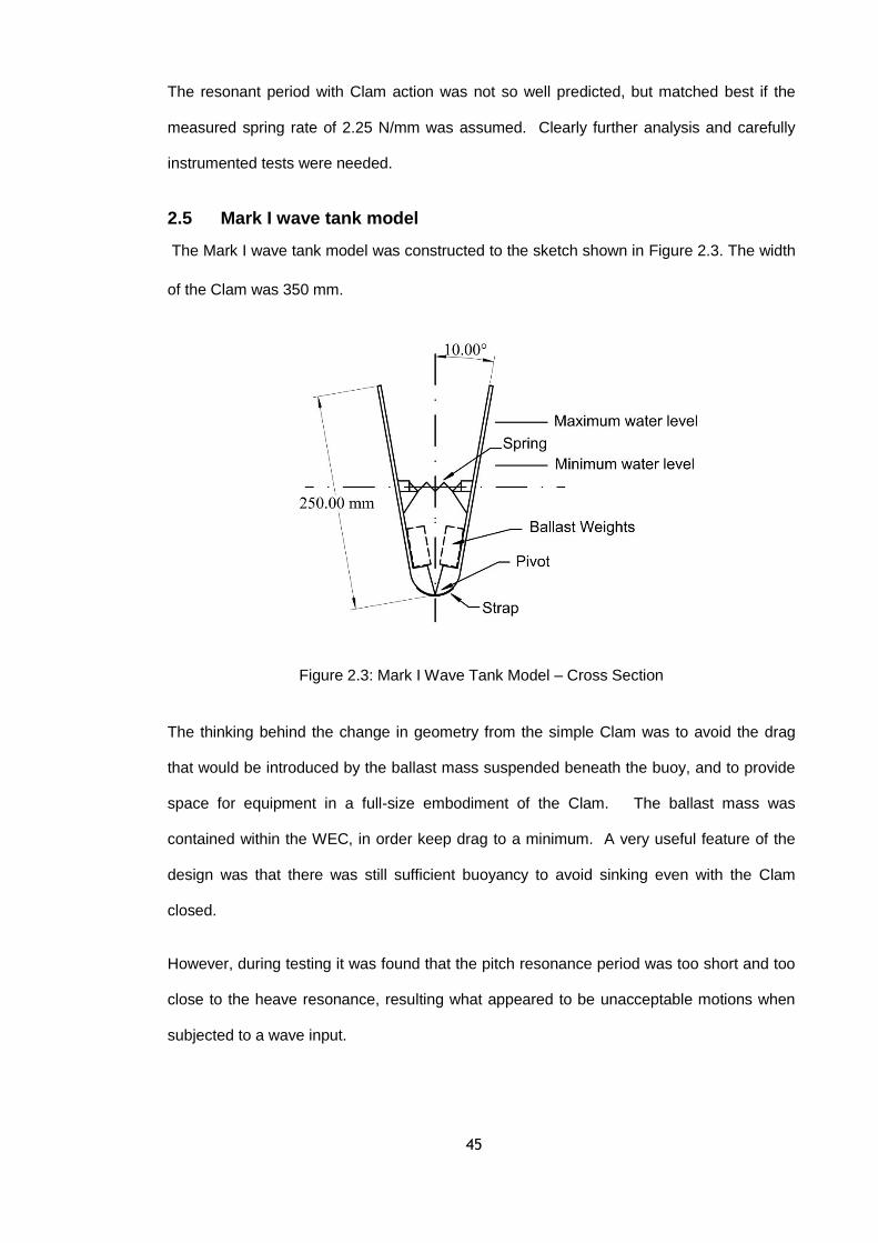
45

The resonant period with Clam action was not so well predicted, but matched best if the

measured spring rate of 2.25 N/mm was assumed. Clearly further analysis and carefully

instrumented tests were needed.

2.5 Mark I wave tank model

The Mark I wave tank model was constructed to the sketch shown in Figure ‎2.3. The width

of the Clam was 350 mm.

Figure ‎2.3: Mark I Wave Tank Model – Cross Section

The thinking behind the change in geometry from the simple Clam was to avoid the drag

that would be introduced by the ballast mass suspended beneath the buoy, and to provide

space for equipment in a full-size embodiment of the Clam. The ballast mass was

contained within the WEC, in order keep drag to a minimum. A very useful feature of the

design was that there was still sufficient buoyancy to avoid sinking even with the Clam

closed.

However, during testing it was found that the pitch resonance period was too short and too

close to the heave resonance, resulting what appeared to be unacceptable motions when

subjected to a wave input.

46

The design was hastily modified in line with Figure ‎2.4.

Figure ‎2.4: Mark I Wave Tank Model with keel

The additional structure consisted of a clear plastic tube into which the ballast weights were

placed, the tube itself being suspended from the upper part of the buoy by cross-braced

cords, designed to provide a rigid connection.

The model then behaved very well in terms of its sea-keeping behaviour in both heave and

pitch. The roll resonance was however found to be a problem – being close to the heave

resonance. In the full-scale device this is likely to be unacceptable, but could be avoided

by ensuring by design that undesirable resonances were well separated from those

resonances needed for good energy capture performance.

A series of still water response tests were also carried out, with the model behaviour being

similar to that of the initial tests.

Spring

Clam sides

Pivot

47

2.6 Mark I wave tank model with bag

The intention behind the wave tank testing carried out at the University of Plymouth at an

early stage in the project was to demonstrate the ability of the Clam to collect power from

sea waves and if possible, to make quantitative measurements of power capture. Francis

Farley suggested that this could be achieved by physical modelling of the system including

the pressurised bag. Hence the Mark I model was modified by enclosing it with a polythene

bag, as shown in Figure ‎2.5.

Figure ‎2.5: Mark I Wave Tank Model plus bag in Plymouth Laboratory

Although the stage was reached where a model, with enclosing bag was trialled, see

Figure ‎2.5, little useful data was obtained. There were three main problems:

Air compressibility effects difficult to scale correctly,

Losses in connecting pipework,

Practical difficulties in making a leak-tight system.

These are further discussed below.

2.6.1 Air compressibility

In order to model the springing effect of the air within the bag it was necessary to connect a

large external reservoir via a flexible tube, as can be seen in the photograph (Figure ‎2.5).

The size of the reservoir was dictated by the need to correctly scale the effect of air

compressibility in the model. The laws of model scaling require that pressure scales as the

scale factor – in this case by a factor of 100. Ideally one would need to scale ambient

48

pressure by a factor of 100. This is physically impractical hence the need to add the

external reservoir. Order of magnitude calculations recently carried out indicate that a

volume of the order of 0.6 m3 would have been needed. Although the scaling implications

were not fully understood at the time of the test, the reservoir had a volume close to this

value.

2.6.2 Losses in connecting pipework

The intention was to measure the power capture by observing the pressure drop across an

orifice plate, placed in the line to the reservoir. In order to restrict the significant losses to

the orifice plate itself the size of the connecting tubing should have been larger than the

size chosen. However it was considered that providing a sufficiently large tube to

overcome the problem of losses would result in a situation where the motion of the device

would be unacceptably compromised, since the internal air pressure in the tube would

render it insufficiently flexible. Hence the proposal to use an alternative method of

simulating the PTO, as described in Section ‎2.7.4.

2.6.3 Building a leak-tight system

Building a leak-tight system was the third area of difficulty, which no doubt could be

overcome with care and the development of suitable manufacturing techniques.

It was decided to build on the experience with the early Clam, by continuing with the use of

polythene sheet. The University has a manual heat sealing press that was used to make

the bag shown in the photograph (Figure ‎2.5). Joining the tube to the bag was a difficult

design problem that was however very successfully overcome in some test samples.

Providing the same degree of sealing on the wave tank model itself was more difficult and

resulted in a minor leak that was however cured to a satisfactory extent with Sellotape.

In addition, during testing it was found that there was a slight leak at the base of the model,

thought to be via pin-holes caused by rough handling. However, the most severe problem

resulted from leaks in the large air reservoir, which was not sufficiently air-tight. The lesson

to be learnt is to aim for a 100% leak-tight system and check it out at each stage while it is

being constructed.

49

2.7 Design and construction of Mark IIa wave tank model

2.7.1 Main assembly

Figure ‎2.6 shows the basic geometry of the Mark IIa wave tank model, which is constructed

almost entirely from acrylic (Perspex).

The hinged sides are made from 15 mm thick acrylic sheet, the thickness being chosen to

provide sufficient depth for screw fixings and to avoid the need for additional stiffening. As

can be seen from the picture (Figure ‎2.7) the device is not enclosed. The Clam sides are

kept apart by the Power Take-Off ram(s) rather than by employing the air pressure inside a

fully enclosing bag. The model scale is 1:50, the width of the Clam being 40 m at full size.

Figure ‎2.6: Basic Geometry of Mark IIa Wave Tank Model

Clam sides

PTO Ram Axis

Pivots

Ballasted Keel

50

Figure ‎2.7 shows the Mark IIa Wave Tank Model ready for testing. The small white

spheres are the targets for the Qualysis motion capture system that logs the Clam’s

position in six degrees of freedom.

Figure ‎2.7: Mark IIa Wave Tank Model ready for testing

Figure ‎2.8 shows the parts of the Clam assembly that are constructed from acrylic sheet

and tube. The Computer Aided Design (CAD) tool, SolidWorks was used to provide both

the manufacturing drawings and the perspective view shown here. The two vertical

members are part of the main body assembly and serve to support the Qualysis targets

that provide data on the position of the main structure, which includes the keel.

Figure ‎2.8: CAD model of Mark IIa Wave Tank Model

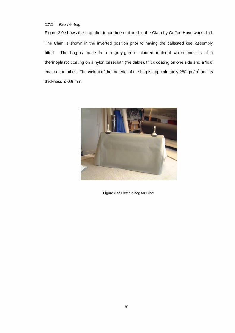
51

2.7.2 Flexible bag

Figure ‎2.9 shows the bag after it had been tailored to the Clam by Griffon Hoverworks Ltd.

The Clam is shown in the inverted position prior to having the ballasted keel assembly

fitted. The bag is made from a grey-green coloured material which consists of a

thermoplastic coating on a nylon basecloth (weldable), thick coating on one side and a ‘lick’

coat on the other. The weight of the material of the bag is approximately 250 gm/m2 and its

thickness is 0.6 mm.

Figure ‎2.9: Flexible bag for Clam

52

2.7.3 Hinge

Figure ‎2.10 shows the hinge diagrammatically. The entire width of the Clam side is shaped

to form a knife edge pivot. A strap completes the assembly – again this runs the whole

width of the Clam side and is constructed of the same material as the bag. Water pressure

holds the Clam side against the main structure.

The hinge has been found to perform its function well. It moves freely and appears friction-

free.

Figure ‎2.10: Hinge Assembly

Strap

Pivot

53

2.7.4 Power Take-Off (PTO)

Figure ‎2.11 shows the principle of operation of the Power Take-Off (PTO). The miniature

hydraulic ram, constructed from a bicycle pump holds the Clam sides apart.

Figure ‎2.11: Power Take-Off Schematic

The whole system is pressurised by the air pressure in the container such that the piston

seal in the ram maintains near leak-free contact.

The orifice plate in the hydraulic line provides the PTO damping while the PTO stiffness is

provided by the compressibility of the air in the reservoir and by the tension spring.

The compressive load in the ram is measured by load cells. Since the hinge friction may

be assumed to be negligible - and the tension spring is friction-free – the result is that all

the damping in the PTO (whether due to the orifice or seal friction) is measured and used in

the calculation of power capture.

Water

Orifice Plate

Pressurised Container

Clam Side

Ram

Tension Spring

Air

54

Much of the testing was carried out with two PTO assemblies in the Clam model, see

Figure ‎2.12 . However testing on the final day of the first set of trials employed a single

PTO assembly.

Figure ‎2.13 contains a photograph of one of the PTO assemblies. Figure ‎2.14 shows the

PTO minus the reservoir and orifice plate, while Figure ‎2.15 shows the plate itself.

Figure ‎2.16 shows the instrumented strut that replaces the PTO for tests where Clam

action is prevented.

Figure ‎2.12: Clam Model - floating

Tension Springs PTO Assemblies

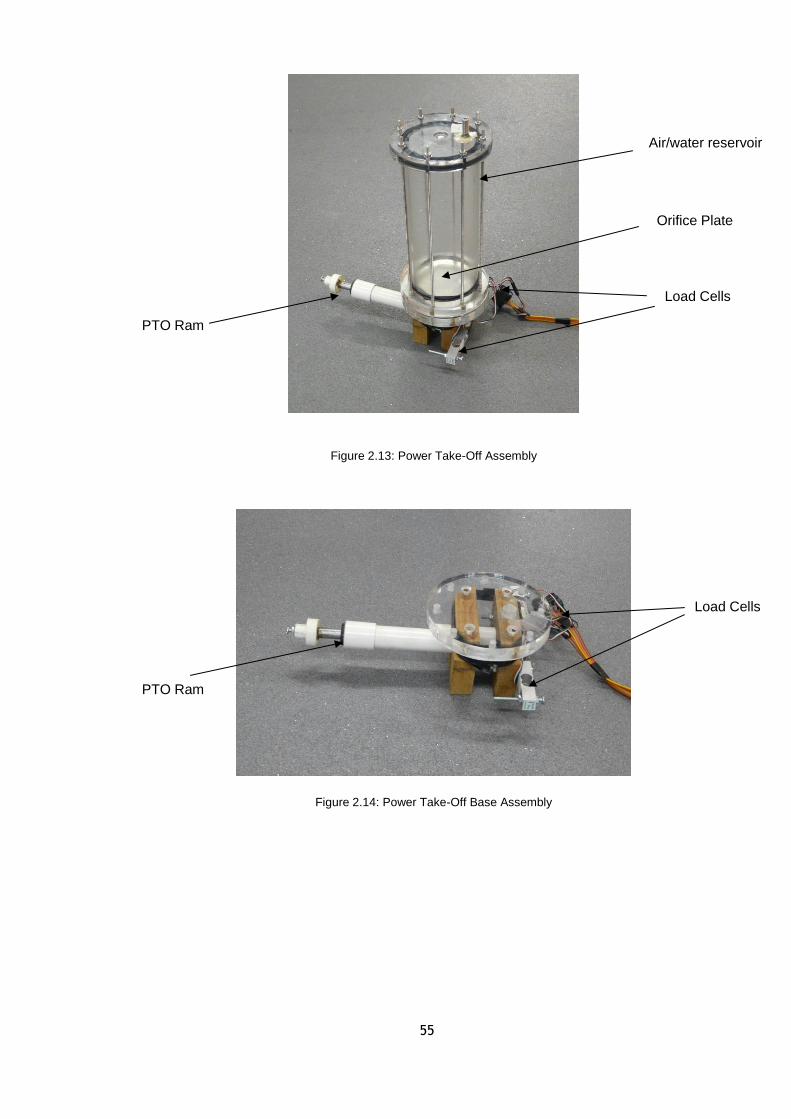
55

Figure ‎2.13: Power Take-Off Assembly

Figure ‎2.14: Power Take-Off Base Assembly

Air/water reservoir

PTO Ram

Load Cells

Orifice Plate

PTO Ram

Load Cells

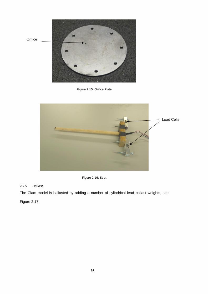
56

Figure ‎2.15: Orifice Plate

Figure ‎2.16: Strut

2.7.5 Ballast

The Clam model is ballasted by adding a number of cylindrical lead ballast weights, see

Figure ‎2.17.

Orifice

Load Cells

57

Figure ‎2.17: Ballast Weights for Clam

There were 7 weights – see Table ‎2.2

Table ‎2.2: Ballast Weights for Mark IIa Model

Weight Identification

Mass, kg

A 4.645

B 4.657

C 4.555

D 4.701

E 4.701

F 2.315

G 2.359

These weights may be placed in two positions – in the keel and in the cradle, as shown in

Figure ‎2.18.

58

Figure ‎2.18: Ballast Weight Positions

2.7.6 Mass properties:

Prior to carrying out the trials the expected mass properties were calculated for each of two

test configurations as shown in Table ‎2.3. Configuration 1 relates to the free-floating WEC

where heave motion is not restrained. Configuration 2 applies to the case where heave

motion is restrained. In this case the WEC is tethered to the floor of the wave tank and the

reduction in the overall mass allows the WEC’s buoyancy to keep the tether taut.

Ballast Weight

Positions

59

Table ‎2.3: Calculated Mass Properties of the Mark IIa Model

Parameter Configuration 1 – free floating

Configuration 2 – heave restrained

Ballast in Cradle, kg 10 0

Ballast in Keel, kg 15 0

Total Model Weight, kg 43.33 18.33

CG posn below CL of upper tube, mm 79 140

CG posn below waterline, mm 319 100

Moment of Inertia about CG, kg m2 , Roll 5.99 0.732

Moment of Inertia about CG, kg m2 , Pitch 3.22 3.499

Moment of Inertia about CG, kg m2 , Yaw 2.4 1.03

Having calculated the expected mass properties (as given in Table ‎2.3), measured mass

properties for the equivalent configurations are given in Table ‎2.4. It can be seen that they

agree closely, namely 43.34 kg versus 43.33 kg for the free floating configuration and 20.08

kg versus 18.33 kg for the heave restrained configuration. The actual model weights for

individual tests varied depending on the precise configuration, such as the number and

position of ballast weights chosen, the number of PTO assemblies used and the quantity of

water in the reservoir(s). However, account has been taken of these variations in the

analysis of the trials.

Table ‎2.4: Measured Mass Properties of the Mark IIa Model

Parameter Configuration 1 – free floating

PTO replaced by fixed length prop

Configuration 2 – fixed in heave

PTO replaced by fixed length prop

Ballast in Cradle, kg 4.701 0

Ballast in Keel, kg 18.558 0

Total Ballast Weight, kg 23.259 0

Weight of wooden prop, kg 0.2 0.2

Weight of Model without Ballast or PTOs, kg

19.88 19.88

Total Model Weight, kg 43.34 20.08

60

2.8 Mark IIb wave tank model

2.8.1 Description of modification

Wave tank testing of the Mark IIa model indicated the need to reduce the friction levels in

the PTO. Consequently a scheme was devised whereby the hydrostatic forces on the

Clam sides were balanced by tension springs as shown in Figure ‎2.19. The springs were

essentially friction-free and allowed the PTO ram to operate at a lower force level, thus

reducing the ram friction since the load on the piston seal was reduced.

The modification involved a pair of cantilevered arms and associated springs. Two

alternative types of springs were incorporated:

Coil springs (Figure ‎2.19) – Mark IIb_1, and

Constant force springs (Figure ‎2.20) – Mark IIb_2.

The constant force springs were of particular significance, since mathematical modelling

indicated that the smaller the PTO stiffness, the greater would be the power capture. In

addition the constant force springs accommodated the full range of movement, whilst the

choice of coil springs was determined by the required force levels and stroke. In

consequence the PTO stiffness when using the coil springs was far from optimal.

61

Figure ‎2.19: Mark IIb_1, Model with coil springs fitted

Figure ‎2.20: Mark IIb_2, Model with constant force springs fitted

Coil springs

PTO assembly Qualysis main body Targets

Constant force

springs

PTO assembly

62

3 Mathematical Modelling

3.1 General

In order to gain an insight into the behaviour of the Clam, Francis Farley developed a series

of single degree of freedom (i.e. 1D in heave) models, programmed in Visual Basic (VBA)

within a spreadsheet (Farley, 2011a) using the theory presented in a confidential note

(Farley, 2011d). A simplified analysis following (Farley, 2011d) that predicts the resonant

period, is presented in Section‎3.2.1.

It should be noted that the effect of viscous drag on the performance of the Clam has not

been included in the theoretical analyses. Drag would normally be expected to reduce the

power capture of the device. However, the practical tests reported in Chapter ‎4

demonstrate good agreement with theoretical predictions even though viscous drag has

been ignored.

3.2 Resonant period and heave stability

3.2.1 Resonant period

Figure ‎3.1: Clam Geometry

𝑥 𝑑𝑥

𝑑𝑤

ℎ

𝜃

𝑤

𝑀

𝑊𝑎𝑡𝑒𝑟 𝑙𝑒𝑣𝑒𝑙

𝐹𝑏 – Buoyancy force 𝐹𝑠 – Spring force 𝑤 – Surface elevation 𝑀 – Mass of buoy 𝑊 – Width of buoy (into paper) 𝜌 – Density of water 𝑔 – Accn due to gravity 𝑘 – Spring stiffness, for spring of length 𝑥 𝐿 – Length of Clam side ℎ – Height of Clam side 𝜃 – Clam semi-angle

𝐿 𝐹𝑏

𝐹𝑠

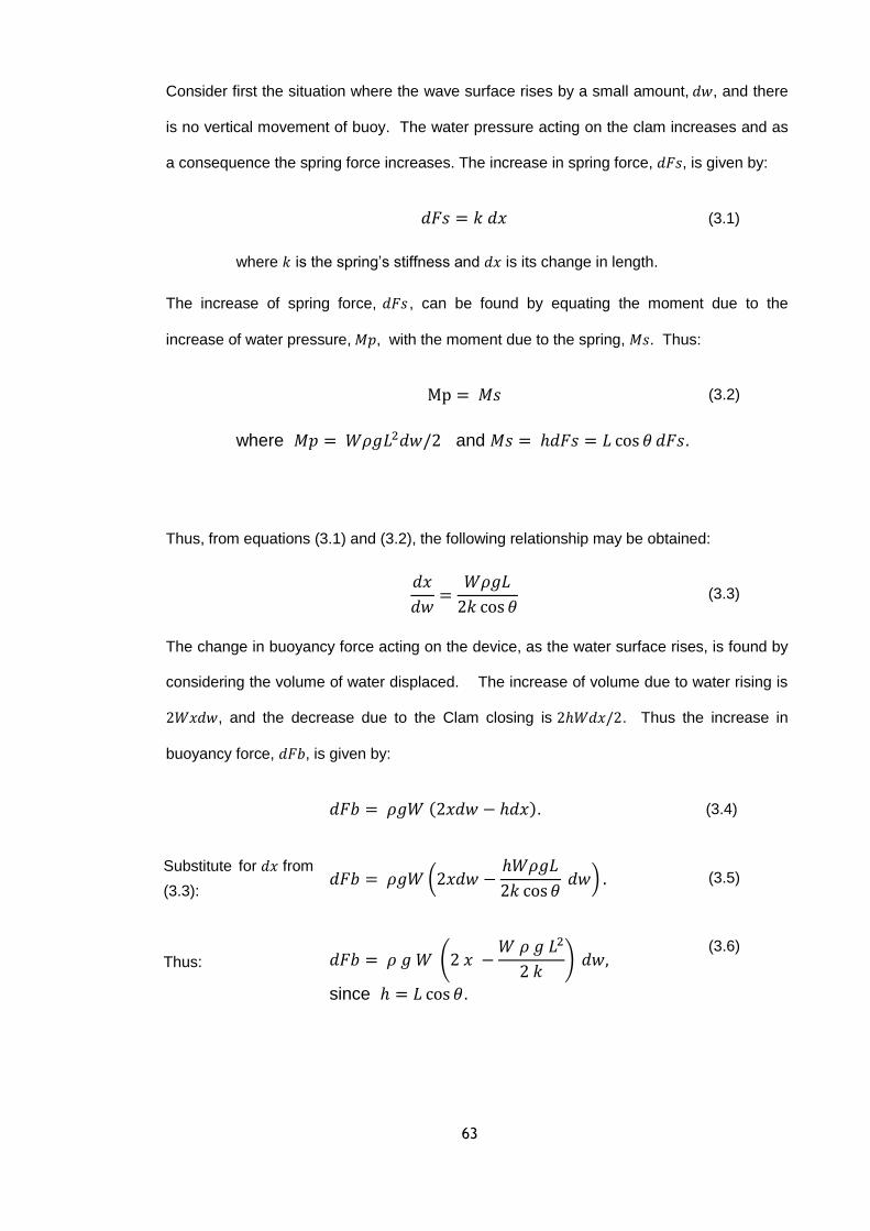
63

Consider first the situation where the wave surface rises by a small amount, 𝑑𝑤, and there

is no vertical movement of buoy. The water pressure acting on the clam increases and as

a consequence the spring force increases. The increase in spring force, 𝑑𝐹𝑠, is given by:

𝑑𝐹𝑠 = 𝑘 𝑑𝑥

where 𝑘 is the spring’s stiffness and 𝑑𝑥 is its change in length.

(‎3.1)

The increase of spring force, 𝑑𝐹𝑠 , can be found by equating the moment due to the

increase of water pressure, 𝑀𝑝, with the moment due to the spring, 𝑀𝑠. Thus:

Mp = 𝑀𝑠

where 𝑀𝑝 = 𝑊𝜌𝑔𝐿2𝑑𝑤/2 and 𝑀𝑠 = ℎ𝑑𝐹𝑠 = 𝐿 cos 𝜃 𝑑𝐹𝑠.

(‎3.2)

Thus, from equations (‎3.1) and (‎3.2), the following relationship may be obtained:

𝑑𝑥

𝑑𝑤=

𝑊𝜌𝑔𝐿

2𝑘 cos 𝜃 (‎3.3)

The change in buoyancy force acting on the device, as the water surface rises, is found by

considering the volume of water displaced. The increase of volume due to water rising is

2𝑊𝑥𝑑𝑤, and the decrease due to the Clam closing is 2ℎ𝑊𝑑𝑥/2. Thus the increase in

buoyancy force, 𝑑𝐹𝑏, is given by:

𝑑𝐹𝑏 = 𝜌𝑔𝑊 (2𝑥𝑑𝑤 − ℎ𝑑𝑥). (‎3.4)

Substitute for 𝑑𝑥 from

(‎3.3): 𝑑𝐹𝑏 = 𝜌𝑔𝑊 (2𝑥𝑑𝑤 −

ℎ𝑊𝜌𝑔𝐿

2𝑘 cos 𝜃 𝑑𝑤) . (‎3.5)

Thus: 𝑑𝐹𝑏 = 𝜌 𝑔 𝑊 (2 𝑥 −

𝑊 𝜌 𝑔 𝐿2

2 𝑘) 𝑑𝑤,

since ℎ = 𝐿 cos 𝜃.

(‎3.6)

64

This equation gives the change of buoyancy force when the water level changes by 𝑑𝑤.

However the relationship is equally valid for the situation where the water level is constant

and the buoy moves by the same amount, i.e. by 𝑑𝑤.

Thus using z to infer vertical motion, and using Newton’s 2nd

law of motion (Accn =

force/mass) we can say that:

𝑑2𝑧

𝑑𝑡2= − 𝜌𝑔𝑊 (2 𝑥 −

𝑊𝜌𝑔𝐿2

2𝑘)

𝑧

𝑀 . (‎3.7)

This is the well-known simple harmonic equation, from which it can be found that the

natural period of resonance, 𝑇, is given by:

𝑇 = 2 𝜋 √𝑀

𝜌 𝑔 𝑊(2 𝑥 −𝜌 𝑔 𝑊 𝐿2

2 𝑘 )

. (‎3.8)

It is important to note that the spring coefficient, 𝑘, applies to a spring of length, 𝑥. Thus in

a lab experiment where use is made of a single spring of coefficient, 𝑘′, then:

𝑘 = 2𝑘′ (‎3.9)

3.2.2 Heave stability

Referring to equation ‎3.8, it can be seen that the denominator of the expression under the

square root sign becomes negative when:

𝜌 𝑔 𝑊 𝐿2

2 𝑘= 2 𝑥 . (‎3.10)

This corresponds to an infinite Natural Period, i.e. the point at which the buoy becomes

unstable in heave, i.e. when:

𝑘 <𝜌 𝑔 𝑊 𝐿2

4 𝑥 . (‎3.11)

65

3.3 AQWA/WAMIT verification

Obtaining the same or similar solution to a problem through the use of more than one

technique (or analysis package) is a standard engineering technique in providing

confidence in the solution. Since AQWA and WAMIT make the same simplifying

assumption of zero viscosity and the same mathematical technique, it is to be expected

that each would give the same solution when presented with the same device geometry.

Having successfully compared WAMIT and AQWA results for some simple shapes it was

then decided to use the geometry of the wave tank model to complete the exercise. All the

hydrodynamic analyses were carried out using the full scale geometry (rather than the

scaled dimensions) as it has been found that this provides a more reliable computation.

Figure ‎3.2 shows the geometry chosen for the analysis.

When using AQWA Workbench, the geometric data for the surface elements are computed

automatically within the software application. Provided the model is represented correctly

on the computer screen, the mathematical definition of the model has a good chance of

being correct. The WAMIT package itself has no graphics capability, but may be used in

conjunction with a graphics package – MultiSurf (AeroHydro, 2012). In the present

instance however it was decided to build the model using a spreadsheet to compute the

geometric data. In order to reduce the scope for error, the model was simplified by omitting

the uprights that connect the keel to the wedge. Two versions of the AWQA model were

constructed – one with and one without the uprights.

66

Figure ‎3.2: Wave Tank Model Geometry for Hydrodynamic Analyses

Figure ‎3.3: AQWA Wave Tank Model – without uprights

Figure ‎3.3 is a screen shot from the Ansys/AQWA modelling package. As can be seen the

uprights have been omitted in order to make the model entirely comparable with the

WAMIT model.

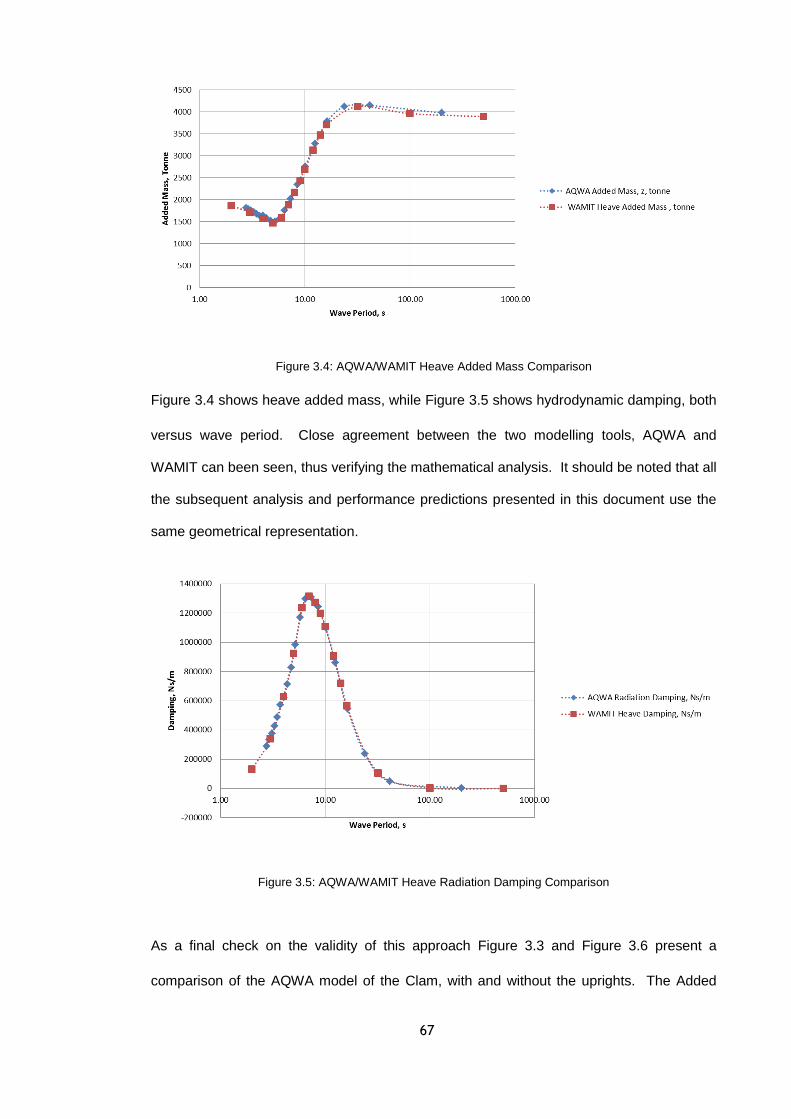
67

Figure ‎3.4: AQWA/WAMIT Heave Added Mass Comparison

Figure ‎3.4 shows heave added mass, while Figure ‎3.5 shows hydrodynamic damping, both

versus wave period. Close agreement between the two modelling tools, AQWA and

WAMIT can been seen, thus verifying the mathematical analysis. It should be noted that all

the subsequent analysis and performance predictions presented in this document use the

same geometrical representation.

Figure ‎3.5: AQWA/WAMIT Heave Radiation Damping Comparison

As a final check on the validity of this approach Figure ‎3.3 and Figure ‎3.6 present a

comparison of the AQWA model of the Clam, with and without the uprights. The Added

68

Mass and Radiation Damping comparisons are shown in Figure ‎3.7 and Figure ‎3.8. The

differences between the two AQWA models are seen to be negligible – so much so that the

plot for the AQWA model without uprights is obscured by the ‘with uprights’ plot. The plots

are to all intents and purposes identical, thus demonstrating that leaving out the uprights in

the WAMIT model is legitimate.

Figure ‎3.6: AQWA Wave Tank Model – with uprights

69

Figure ‎3.7: AQWA Wave Tank Model comparison – Added Mass

Figure ‎3.8: AQWA Wave Tank Model comparison – Radiation Damping

70

3.4 Generalised Mode applied to Clam action

As has been explained earlier (see Section ‎1.4.1) WAMIT allows a “deformable body” to be

analysed using “Generalized Body Modes”. The method is explained in the WAMIT User

Guide (WAMIT 2012), and Newman (Newman, 1994).

Figure ‎3.9: Definition of Mode 7

The two sides of the Clam move towards and away from each other, being hinged at their

lower ends. This hinged action is the only ‘generalised mode’ and therefore becomes

mode 7, the first 6 modes being the conventional rigid body modes. Modes 1 to 3 describe

translational motion in the x, y, z (surge, sway and heave) axes respectively and rotation

about the x, y, and z axes (roll, pitch and yaw) is described by modes 4, 5 and 6. Mode 7 is

known as the Clam mode and is defined by the movement of the PTO ram, as shown in

Figure ‎3.9 - the positive direction of movement being shown by the arrows. Note that the

models used in this thesis utilise modes 3 and 7, alone i.e. mode 3, heave, and mode 7, the

Clam mode.

By defining the mode in terms of the movement of the PTO ram the result is that the mode

7 force and displacement are identically the same as the PTO force and displacement.

Consequently the values of PTO stiffness and damping may be applied to the Clam mode

(mode 7) without modification.

71

The quantities, VELH and ZDISP, need to be computed at all relevant panel vertices in

relation to a ‘unit displacement’ (i.e. a displacement of unity) of the PTO ram, the positive

direction of these quantities being shown in Figure ‎3.9. VELH is the displacement normal

to the surface (+ve into the body) and ZDISP is the vertical (Z-direction) displacement.

Accordingly the FORTRAN code to compute VELH and ZDISP is incorporated into the

FORTRAN subroutine NEWMODES (actually ‘newmodes.f’). To complete the model

preparation a ‘.dll’ file needs to be compiled.

Computing VELH and ZDISP at each panel vertex is not straightforward, since the Clam

pivot is not in line with the outer surface of the Clam. The trigonometric formulae to

compute for VELH and ZDISP were thus coded and included in the NEWMODES

subroutine. As a precaution the computation was carefully checked using a CAD package.

As previously mentioned, a spreadsheet was used to produce the geometric data file for

WAMIT, using the most basic type of element, namely the flat quadrilateral panel, as

specified in the WAMIT control files as the “Low Order” panel method.

Although WAMIT should allow the origin to be positioned below the water surface, it was

found necessary to put the origin for the axis system on the waterline. The geometric data

initially took the vertex of the Clam as a datum. However, this produced results that were

clearly in error when attempting to incorporate the Clam mode. After some experimentation

with a different analysis option (i.e. the pre-processor program DEFMOD), the most

satisfactory approach proved to be the use of the NEWMODES option to model the Clam

mode, with the axes origin at the waterline.

Preliminary testing of the model produced results that appeared at first sight to be incorrect

- and in fact proved to be so. The model predicted the behaviour shown in Figure ‎3.10, and

discussed more fully below. The concern was that the NEWMODES approach did not

correctly compute the hydrostatic coefficients and it was suspected that this was due to the

fact that the NEWMODES program code does not completely compute the coefficients

when the surface stretches. The mathematics behind this is described in the WAMIT User

72

Guide (WAMIT, 2012), Chapter 9, 2012) and by (Newman, 1994). Thus the hydrostatic

coefficient, 𝐶𝑖𝑗 , may be calculated by equation ‎3.12 which is reproduced from the WAMIT

User Guide (WAMIT, 2012), equation 9.11.

𝐶𝑖𝑗 = 𝜌𝑔 ∬ 𝑛𝑗(

𝑆𝑏

𝑤𝑖 + 𝑧𝐷𝑖)𝑑𝑆

where 𝐶𝑖𝑗 is the force component for generalised mode ‘𝑖’ due

to unit displacement of the body in mode ‘𝑗’.

For definitions of the other parameters refer to (WAMIT, 2012)

and (Newman, 1994).

(‎3.12)

The User Guide (WAMIT, 2012) states that the first term within the brackets is calculated

within WAMIT if “newmodes.dll” is used, while the second term, involving the Divergence of

the surface displacement vector, is not. Advice was taken from the WAMIT developers

who explained that this second part only applies when the surface is stretched. Although

the Clam surface is in effect “stretched” as the Clam moves, they advised that this is a

minor effect and may be ignored.

A typical, but erroneous output from the WAMIT/NEWMODES analysis is shown in

Figure ‎3.10. Firstly, the PTO response shows a dip near to the resonant peak of the heave

motion which was not expected. Secondly it would be expected that the heave amplitude

would become equal to the wave amplitude for long period waves – and this did not occur.

73

Figure ‎3.10: Incorrectly predicted Clam response

When the model was physically tested in the wave tank it became clear that the analysis

was indeed incorrect. The most likely source was an error in the calculation of the

hydrostatic coefficients, 𝐶𝑖𝑗 , within the WAMIT-supplied NEWMODES program code.

An alternative method of calculating the hydrostatic coefficients was then devised, resulting

in response predictions in line with model tests and expectations, as shown in Figure ‎3.11,

which is based on the analysis of Trial 2, see Table ‎4.1.

Figure ‎3.11: Improved prediction of Clam response

74

The method of calculating the hydrostatic coefficients is now described, taking as an

example the Cross Coupled Hydrostatic Coefficient, 𝐶73. This is given by the change in

PTO/Clam force (i.e. mode 7) due to a unit heave displacement of the device (i.e. mode 3).

Thus:

𝐶73 =𝑑𝐹

𝑑ℎ

where 𝐹 is the PTO load and ℎ is the vertical distance from the Clam

pivot to the waterline.

(‎3.13)

It can readily be shown that 𝐹 is given by:

𝐹 =𝜌𝑔𝑊ℎ3

6𝑍𝑐𝑜𝑠2𝜃

where 𝜌 is density of water, 𝑔 is the acceleration due to gravity, 𝑍 is

the vertical distance from the Clam pivot to the line of action of the

PTO ram, 𝑊 is the width of the WEC and 𝜃 is the Clam semi-angle

(‎3.14)

Thus:

𝐶73 =𝜌𝑔𝑊ℎ2

2𝑍𝑐𝑜𝑠2𝜃 (‎3.15)

A similar approach was used to calculate values for all the hydrostatic coefficients.

3.5 WAMIT analysis

WAMIT modelling followed the methodology and examples given in the user manual

(WAMIT, 2012), using the flat lower order quadrilateral surface element throughout the

analysis. The model input included data files to specify the calculation options, control the

progress of the computation and specify the required output data files. Also required were

files to define the model geometry and externally applied stiffness and damping.

75

The geometric input data was computed using a spreadsheet, verified by the method

described in Section ‎3.3. The output data contained the calculated response to the various

wave input data, and also included data files of hydrodynamic coefficients.

As will be described in Section ‎3.6, the hydrodynamic coefficients were curve-fitted for use

in the frequency domain model, thus allowing the model behaviour to be assessed at any

particular wave period.

For full details of the WAMIT analysis, reference should be made to Appendix B.

3.6 Frequency domain model

The development of the modelling suite moved to the use of a mathematical package,

Mathcad (PTC, 2014) to carry out further frequency domain modelling, the main reason

being to facilitate the efficient production of performance curves – to study the effect of

changes to PTO stiffness and damping and also look at the effect of restraining the device

in heave.

Once the hydrodynamic coefficients were known, then quantities such as the heave and

Clam response and power capture could be calculated by straightforward linear algebraic

equations. Thus the approach taken in the Mathcad modelling was to curve-fit the

hydrodynamic data, using cubic splines, so that accurate figures for the data might be

computed for any chosen wave period.

A particular advantage of this approach is that the output data may be plotted as smooth

curves, and any particular point of interest, such as a resonant peak may be identified.

Table ‎3.1 lists the hydrodynamic parameters that are curve-fitted.

76

Table ‎3.1: Hydrodynamic Parameters that are Curve Fitted

Parameter Description Parameter Description

𝐴33 Heave Added Mass 𝜎33 Argument of Haskinds Exciting Force in Heave

𝐵33 Heave Damping 𝑀𝑜𝑑33 Modulus of Haskinds Exciting Force in Heave

𝑀33 Device Mass 𝜎77 Argument of Haskinds Exciting Force for Clam

Mode

𝐴77 Clam Added Mass 𝑀𝑜𝑑77 Modulus of Haskinds Exciting Force for Clam

Mode

𝐵77 Clam (Added) Damping

𝐴37 Cross Coupled (3,7) Added Mass

𝐵37 Cross Coupled (3,7) Damping



Table ‎3.2 lists the hydrostatic parameters that are constant, i.e. not a function of wave

period:

Table ‎3.2: Hydrostatic Parameters


𝐶33 Heave Hydrostatic Coefficient 𝐶37 Cross Coupled (3,7) Hydrostatic Coefficient

𝐶77 Clam Hydrostatic Coefficient 𝐶73 Cross Coupled (7,3) Hydrostatic Coefficient

The following data is input to the calculation:

Table ‎3.3: Input Data


𝑀33 Device Mass

𝐵33𝐸 Externally Applied Heave Damping 𝐵77

𝐸 PTO Damping

𝐶33𝐸 Externally Applied Heave Stiffness 𝐶77

𝐸 PTO Stiffness

77

Note that the parameters are appropriately scaled within the Mathcad model, in accordance

with the scaling factors in the User Manual (WAMIT, 2012), such that the calculations are

carried out in real units. This is good engineering practice and through dimensional

analysis proves to be most helpful in tracing errors.

Equation ‎3.16 describes the equation of motion that WAMIT solves - see the WAMIT User

Guide, Section 3.4.

∑[−𝜔2(𝑀𝑖𝑗 + 𝑀𝑖𝑗𝐸 + 𝐴𝑖𝑗) + 𝑖𝜔(𝐵𝑖𝑗 + 𝐵𝑖𝑗

𝐸 ) + (𝐶𝑖𝑗 + 𝐶𝑖𝑗𝐸)]

7

𝑗=1

𝜉𝑗 = 𝑋𝑖 (‎3.16)

where 𝜉𝑗 is the displacement in the jth degree of freedom caused by the force 𝑋𝑖.

This is implemented in the frequency domain model for just two degrees of freedom i.e.

heave (mode 3) and the Clam or PTO mode (mode 7). Equations ‎3.17 to ‎3.26 show the

process.

𝑋 33 = 𝑀𝑜𝑑33(𝑐𝑜𝑠(𝜎33) + 𝑗𝑠𝑖𝑛 (𝜎33)) (‎3.17)

𝑋 77 = 𝑀𝑜𝑑77(𝑐𝑜𝑠(𝜎77) + 𝑗𝑠𝑖𝑛 (𝜎77)) (‎3.18)

𝑍 33 = −𝜔2(𝑀33 + 𝐴33) + 𝑗𝜔(𝐵33 + 𝐵33𝐸 ) + (𝐶33 + 𝐶33

𝐸 ) (‎3.19)

𝑍 37 = −𝜔2𝐴37 + 𝑗𝜔𝐵37 + 𝐶37 (‎3.20)

𝑍 73 = −𝜔2𝐴73 + 𝑗𝜔𝐵73 + 𝐶73 (‎3.21)

𝑍 77 = −𝜔2𝐴77 + 𝑗𝜔(𝐵77 + 𝐵77𝐸 ) + (𝐶77 + 𝐶77

𝐸 ) (‎3.22)

where 𝜔 is the wave radian frequency (=2𝜋

𝑊𝑎𝑣𝑒 𝑃𝑒𝑟𝑖𝑜𝑑), and

𝑍 33, 𝑍 37, 𝑍 73 and 𝑍 77 are complex stiffnesses.

(‎3.23)

78

Expanding this in matrix form for the two degrees of freedom under consideration (i.e.

modes 3 and 7), gives:

[𝑍 33 𝑍 37

𝑍 73 𝑍 77].[

𝜉3 𝜉7

] = [𝑋 33

𝑋 77] (‎3.24)

Or [𝑍].[𝜉] = [𝑋] (‎3.25)

The displacements [𝜉] are solved by inverting [𝑍] and pre-multiplying equation ‎3.25, so

that:

[𝜉] = [𝑍]−1.[𝑋] (‎3.26)

𝜉3 and 𝜉7 are the heave and Clam complex displacements that contain the amplitude and

phase information for modes 3 (heave) and 7 (Clam). Thus the heave and Clam

amplitudes may be readily computed.

As a check on the accuracy of calculation, the heave and Clam amplitudes calculated by

the frequency domain model and by WAMIT were compared at a chosen wave period.

Table ‎3.4 shows the result, and as can be seen the figures are the same, which is

expected, since the calculation in the frequency domain model uses WAMIT data and the

same mathematical formulae. This demonstrated that the conversion to the frequency

domain model had been carried out correctly and was error-free.

Table ‎3.4: Comparison of WAMIT and Mathcad frequency domain model outputs

Heave amplitude (mode 3), m

Clam amplitude (mode 7), m

WAMIT output at 6 s period 0.20149 0.65948

Mathcad frequency domain model output at 6 s period

0.20149 0.65948

79

The power capture is calculated within the Mathcad frequency domain model using

equation ‎3.27:

𝑃 =1

2𝐵77

𝐸 |𝜉7|2𝜔2 . (‎3.27)

where 𝑃 is the Power Capture, 𝐵77𝐸 is the PTO damping, 𝜉7 is the complex PTO (= Clam)

amplitude and 𝜔 is the radian wave frequency.

Note that much use is made of the acronym RAO or Response Amplitude Operator (RAO).

This dimensionless quantity relates the amplitude of the chosen parameter to the wave

amplitude as indicated by equation ‎3.28:

𝑅𝐴𝑂3 =|𝜉3|

𝑎 and 𝑅𝐴𝑂7 =

|𝜉7|

𝑎 , (‎3.28)

where 𝑅𝐴𝑂3 is the heave RAO, 𝑅𝐴𝑂7 is the Clam or PTO RAO, |𝜉3| and |𝜉7| are the moduli

of the heave and PTO amplitudes and 𝑎 is the wave amplitude.

Thus equation ‎3.27 may be re-written:

𝑃 =1

2𝐵77

𝐸 𝑅𝐴𝑂72 𝑎2 𝜔2 . (‎3.29)

Using Mathcad to host the frequency domain model had several advantages over the use

of the WAMIT model alone. Due having curve-fitted the hydrodynamic data, the Clam’s

behaviour could be predicted for any selected wave period – or range of wave periods. In

addition the computing time was shorter and output files suitable for input to the time

domain model could be generated easily. One further significant practical advantage was

that the frequency domain model could be used after the WAMIT licence period had

expired.

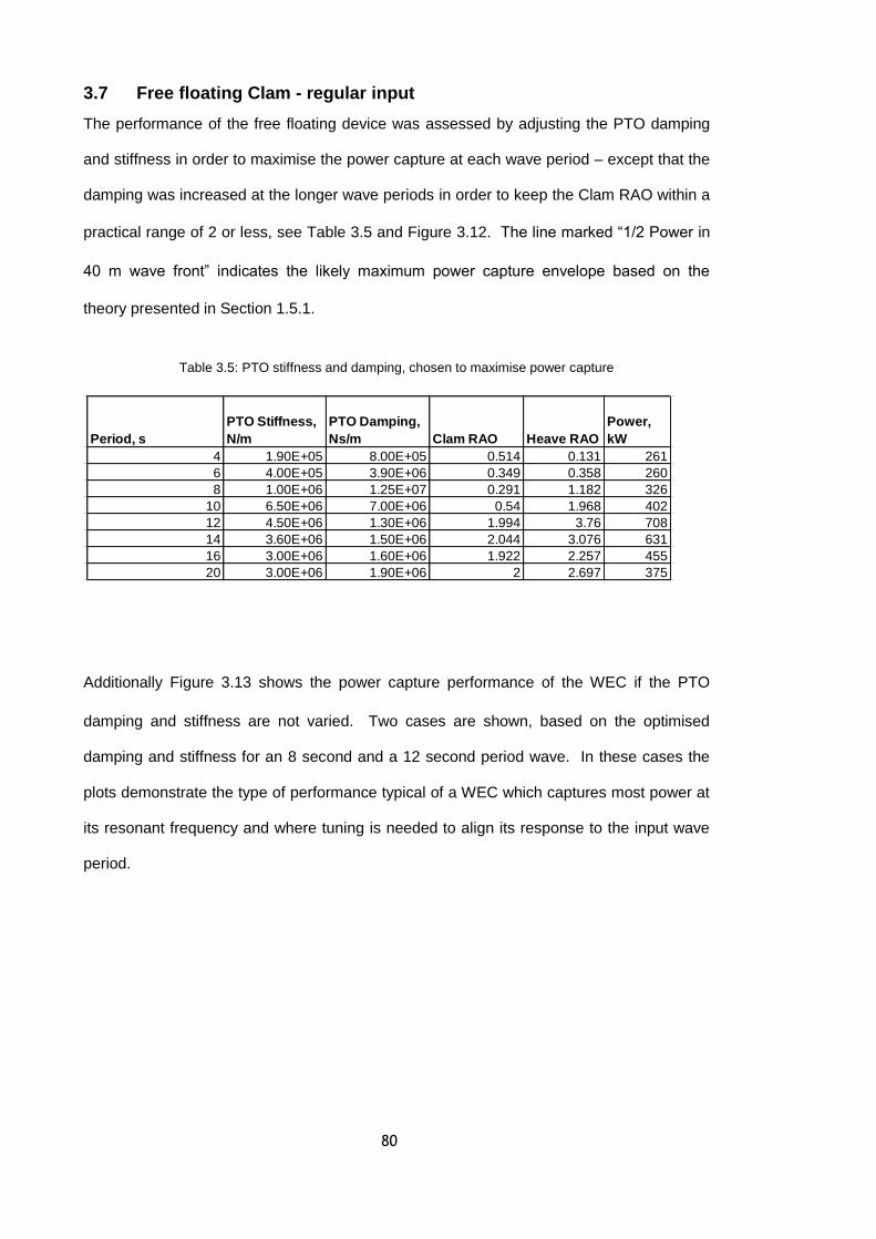
80

3.7 Free floating Clam - regular input

The performance of the free floating device was assessed by adjusting the PTO damping

and stiffness in order to maximise the power capture at each wave period – except that the

damping was increased at the longer wave periods in order to keep the Clam RAO within a

practical range of 2 or less, see Table ‎3.5 and Figure ‎3.12. The line marked “1/2 Power in

40 m wave front” indicates the likely maximum power capture envelope based on the

theory presented in Section ‎1.5.1.

Table ‎3.5: PTO stiffness and damping, chosen to maximise power capture

Additionally Figure ‎3.13 shows the power capture performance of the WEC if the PTO

damping and stiffness are not varied. Two cases are shown, based on the optimised

damping and stiffness for an 8 second and a 12 second period wave. In these cases the

plots demonstrate the type of performance typical of a WEC which captures most power at

its resonant frequency and where tuning is needed to align its response to the input wave

period.

Free Floating - no heave restriction Clam RAO controlled by increased PTO damping

Period, s

PTO Stiffness,

N/m

PTO Damping,

Ns/m Clam RAO Heave RAO

Power,

kW

4 1.90E+05 8.00E+05 0.514 0.131 261

6 4.00E+05 3.90E+06 0.349 0.358 260

8 1.00E+06 1.25E+07 0.291 1.182 326

10 6.50E+06 7.00E+06 0.54 1.968 402

12 4.50E+06 1.30E+06 1.994 3.76 708

14 3.60E+06 1.50E+06 2.044 3.076 631

16 3.00E+06 1.60E+06 1.922 2.257 455

20 3.00E+06 1.90E+06 2 2.697 375

hydrostatic coefficients.

81

Figure ‎3.12: Power Capture for Free Floating device - 1

Figure ‎3.13: Power Capture for Free Floating device - 2

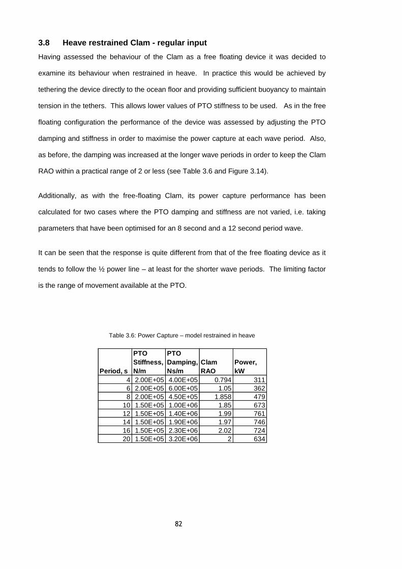
82

3.8 Heave restrained Clam - regular input

Having assessed the behaviour of the Clam as a free floating device it was decided to

examine its behaviour when restrained in heave. In practice this would be achieved by

tethering the device directly to the ocean floor and providing sufficient buoyancy to maintain

tension in the tethers. This allows lower values of PTO stiffness to be used. As in the free

floating configuration the performance of the device was assessed by adjusting the PTO

damping and stiffness in order to maximise the power capture at each wave period. Also,

as before, the damping was increased at the longer wave periods in order to keep the Clam

RAO within a practical range of 2 or less (see Table 3.6 and Figure 3.14).

Additionally, as with the free-floating Clam, its power capture performance has been

calculated for two cases where the PTO damping and stiffness are not varied, i.e. taking

parameters that have been optimised for an 8 second and a 12 second period wave.

It can be seen that the response is quite different from that of the free floating device as it

tends to follow the ½ power line – at least for the shorter wave periods. The limiting factor

is the range of movement available at the PTO.

Table ‎3.6: Power Capture – model restrained in heave

No Heave, BUT with increased PTO damping to reduce Clam RAO

Period, s

PTO

Stiffness,

N/m

PTO

Damping,

Ns/m

Clam

RAO

Power,

kW

4 2.00E+05 4.00E+05 0.794 311

6 2.00E+05 6.00E+05 1.05 362

8 2.00E+05 4.50E+05 1.858 479

10 1.50E+05 1.00E+06 1.85 673

12 1.50E+05 1.40E+06 1.99 761

14 1.50E+05 1.90E+06 1.97 746

16 1.50E+05 2.30E+06 2.02 724

20 1.50E+05 3.20E+06 2 634

83

Figure ‎3.14: Power Capture – model restrained in heave - 1

Figure ‎3.15: Power Capture for model restrained in heave – 2

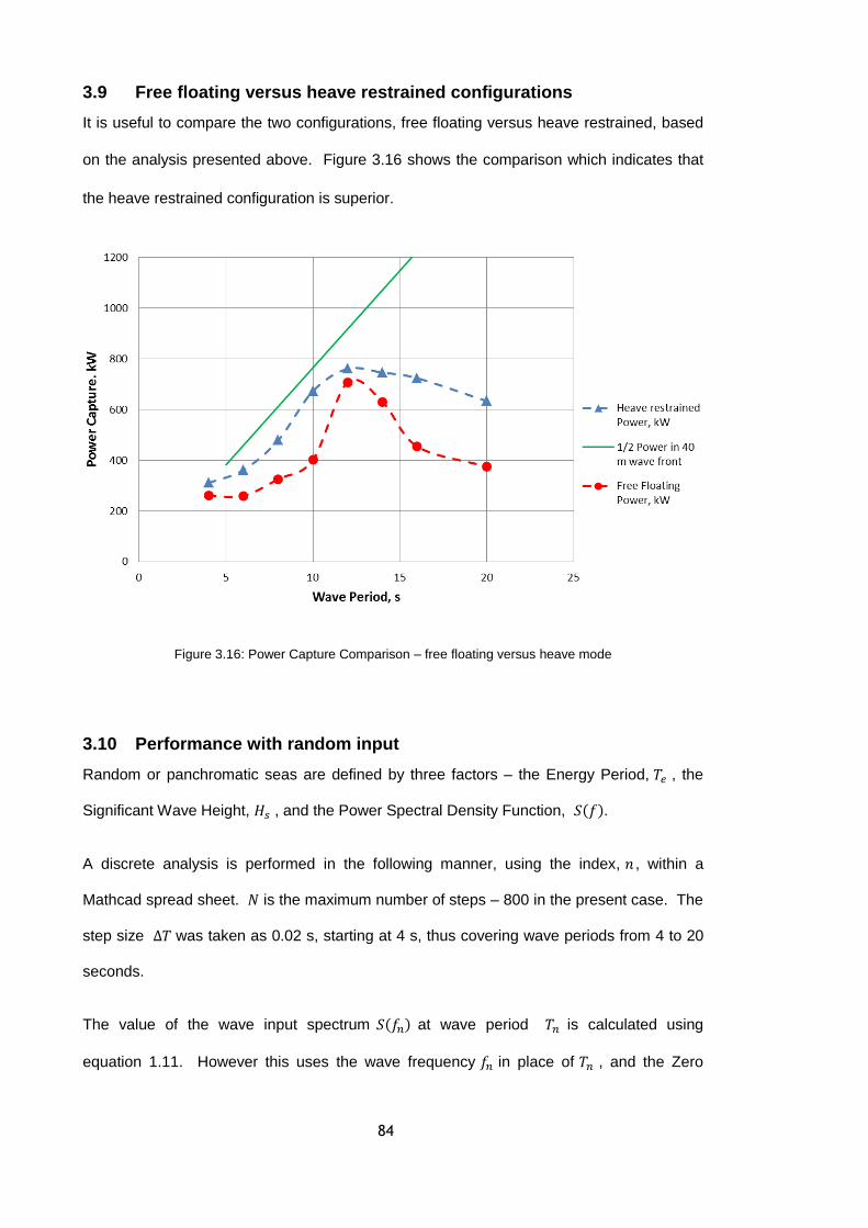
84

3.9 Free floating versus heave restrained configurations

It is useful to compare the two configurations, free floating versus heave restrained, based

on the analysis presented above. Figure ‎3.16 shows the comparison which indicates that

the heave restrained configuration is superior.

Figure ‎3.16: Power Capture Comparison – free floating versus heave mode

3.10 Performance with random input

Random or panchromatic seas are defined by three factors – the Energy Period, 𝑇𝑒 , the

Significant Wave Height, 𝐻𝑠 , and the Power Spectral Density Function, 𝑆(𝑓).

A discrete analysis is performed in the following manner, using the index, 𝑛 , within a

Mathcad spread sheet. 𝑁 is the maximum number of steps – 800 in the present case. The

step size ∆𝑇 was taken as 0.02 s, starting at 4 s, thus covering wave periods from 4 to 20

seconds.

The value of the wave input spectrum 𝑆(𝑓𝑛) at wave period 𝑇𝑛 is calculated using

equation ‎1.11. However this uses the wave frequency 𝑓𝑛 in place of 𝑇𝑛 , and the Zero

85

Crossing Period, 𝑇𝑧 , rather than the Energy Period, 𝑇𝑒 , so the following adjustments are

made:

𝑓𝑛 =

1

𝑇𝑛

(‎3.30)

where 𝑛 = 0 𝑡𝑜 𝑁 (‎3.31)

and 𝑇𝑧 =

𝑇𝑒

1.20265

(‎3.32)

The Power 𝑃𝑛 at each wave period, 𝑇𝑛 , is calculated from equation ‎3.27.

At each step the incremental contribution to the power capture ∆𝑃𝑛 is obtained from the

following equation:

∆𝑃𝑛 = 2𝑃𝑛 𝑆(𝑓𝑛)∆𝑓𝑛 (‎3.33)

where ∆𝑓𝑛 =

∆𝑇

(𝑇𝑛(𝑇𝑛 + ∆𝑇))

(‎3.34)

The total power capture is found from equation ‎3.35:

𝑃 = ∑∆𝑃𝑛

𝑎2

𝑁

𝑛=0

(‎3.35)

where the wave amplitude, 𝑎, is usually taken as unity, i.e. 1 m, but if a different figure is

chosen, then this is allowed for in equation ‎3.35.

As an example, consider the configuration described in Table ‎3.6, optimised for a 10

second wave period, i.e. where the PTO stiffness is 0.15 MN/m and the PTO damping is

1 MNs/m. If the Energy Period 𝑇𝑒 is taken as 10 seconds and the Significant Wave Height

𝐻𝑠 as 2 m, the computed mean power capture is then 335 𝑘𝑊. The incident wave power

86

over a 40 m wave front is 765 kW (Equation ‎1.9), and following the logic adopted

throughout this document, a figure of 382 kW (i.e. half of 765 kW) may be considered a

practical maximum. 335 kW is 0.88 of 382 kW – a good result.

Note that the performance data throughout this report are based on the use of fresh water,

which has a density of 1000 kg/m3, as opposed to sea water with a density of 1025 kg/m

3.

The only exception is the analysis of Appendix D, where the Clam’s performance at Wave

Hub is estimated.

3.11 Time domain model description

3.11.1 General

Time domain modelling of the Clam employs the VisSim continuous systems modelling tool

to provide a time domain simulation of the motion of the device. A number of numerical

integration techniques are available within VisSim. However, the Runge Kutta 4th order

integration option has been used for all the simulations, generally with a time step of 0.05 s.

In common with all the mathematical modelling carried out on this project, full scale values

of all parameters are used. The model is restricted to modelling just the Heave and the

Clam motion.

A block diagram is constructed, using the PC monitor, with arithmetic and logical functions

being implemented by interconnecting the relevant basic level blocks, such as add,

multiply, etc. Other blocks are used to provide inputs, such as ramps, sine, steps etc. A

range of output blocks provide on-screen plots and output to text files. Compound Blocks,

containing these basic level block diagrams are employed to organise the model into a

manageable form on the screen. Compound blocks may be placed within further higher

level Compound Blocks. Figure ‎3.17 shows the block diagram at the highest level.

87

Figure ‎3.17: Time domain model - Top level Block Diagram

The algorithms within each high level block are described in the following sections.

3.11.2 PTO and Heave Stiffness & Damping

This block simply inputs the chosen values of externally applied PTO and Heave damping

and stiffness as listed in Table ‎3.7.

Table ‎3.7: Stiffness and damping parameters for input to the time domain model.


𝐵33𝐸 Externally Applied Heave Damping 𝐵77

𝐸 PTO Damping

𝐶33𝐸 Externally Applied Heave Stiffness 𝐶77

𝐸 PTO Stiffness

88

Hydrodynamic and hydrostatic coefficients, plus the wave period, 𝑇, and device mass, 𝑀33,

are computed by the frequency domain model (Section ‎3.6) for input to the time domain

model. The relevant parameters are listed in Table ‎3.8.

Table ‎3.8: Hydrodynamic and hydrostatic coefficients


𝑇 Wave Period 𝑀33 Device Mass



𝜎33 Argument of Haskinds Exciting Force in Heave

𝜎77 Argument of Haskinds Exciting Force for Clam Mode



𝐴33 Heave Added Mass 𝐵33 Heave Damping

𝐴77 Clam Added Mass 𝐵77 Clam (Added) Damping





𝐶33 Heave Hydrostatic Coefficient 𝐶37 Cross Coupled (3,7) Hydrostatic Coefficient

𝐶77 Clam Hydrostatic Coefficient 𝐶73 Cross Coupled (7,3) Hydrostatic Coefficient

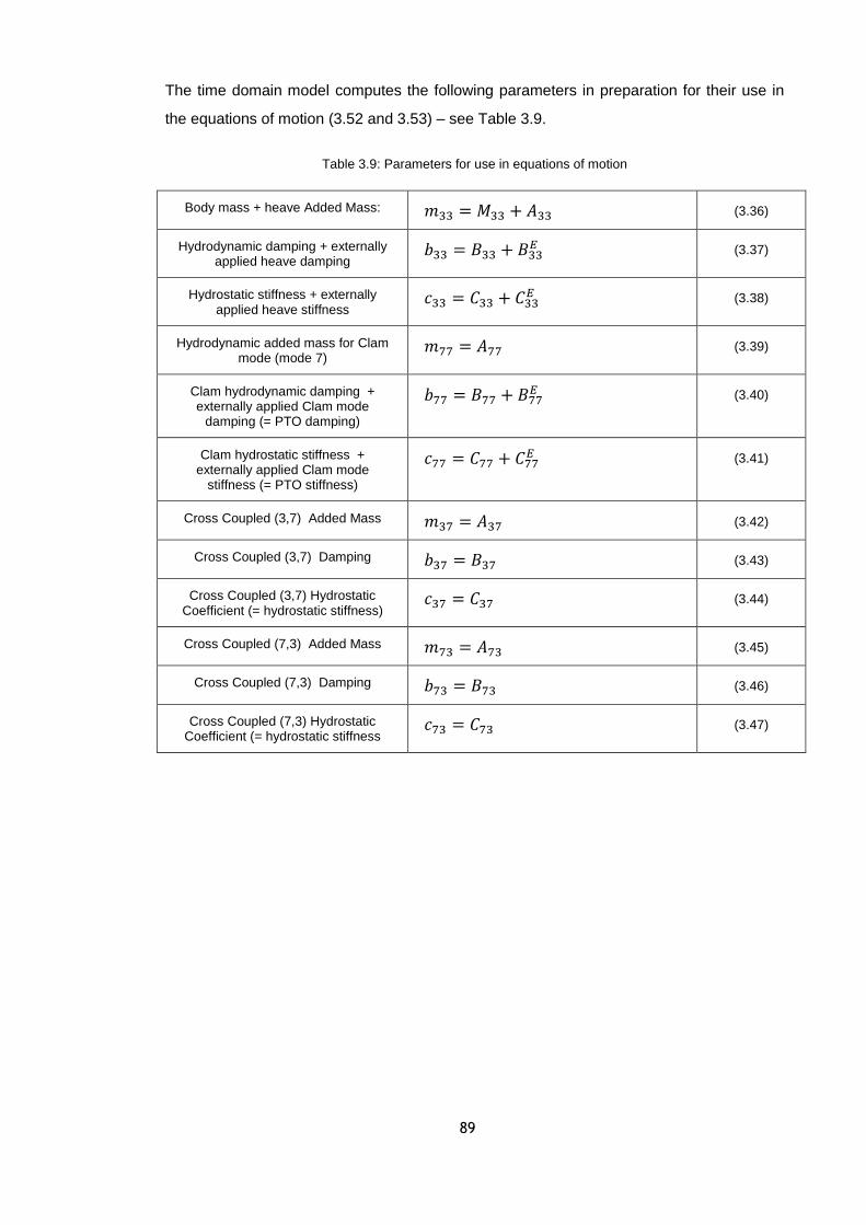
89

The time domain model computes the following parameters in preparation for their use in

the equations of motion (‎3.52 and ‎3.53) – see Table ‎3.9.

Table ‎3.9: Parameters for use in equations of motion

Body mass + heave Added Mass: 𝑚33 = 𝑀33 + 𝐴33 (‎3.36)

Hydrodynamic damping + externally applied heave damping

𝑏33 = 𝐵33 + 𝐵33𝐸 (‎3.37)

Hydrostatic stiffness + externally applied heave stiffness

𝑐33 = 𝐶33 + 𝐶33𝐸 (‎3.38)

Hydrodynamic added mass for Clam mode (mode 7)

𝑚77 = 𝐴77 (‎3.39)

Clam hydrodynamic damping + externally applied Clam mode

damping (= PTO damping)

𝑏77 = 𝐵77 + 𝐵77𝐸 (‎3.40)

Clam hydrostatic stiffness + externally applied Clam mode

stiffness (= PTO stiffness)

𝑐77 = 𝐶77 + 𝐶77𝐸 (‎3.41)

Cross Coupled (3,7) Added Mass 𝑚37 = 𝐴37 (‎3.42)

Cross Coupled (3,7) Damping 𝑏37 = 𝐵37 (‎3.43)

Cross Coupled (3,7) Hydrostatic Coefficient (= hydrostatic stiffness)

𝑐37 = 𝐶37 (‎3.44)

Cross Coupled (7,3) Added Mass 𝑚73 = 𝐴73 (‎3.45)

Cross Coupled (7,3) Damping 𝑏73 = 𝐵73 (‎3.46)

Cross Coupled (7,3) Hydrostatic Coefficient (= hydrostatic stiffness

𝑐73 = 𝐶73 (‎3.47)

90

3.11.3 Integration engine

The inputs to the Integration Engine are the second derivatives 𝛿3̈ and 𝛿7̈ of the heave

and Clam displacements, respectively. These are then integrated with respect to time, 𝑡,

as follows:

Heave velocity, �̇�3 = ∫ 𝛿3 𝑑𝑡̈ (‎3.48)

Heave position, 𝛿3 = ∫ �̇�3 𝑑𝑡 (‎3.49)

Clam velocity, �̇�7 = ∫ 𝛿7̈ 𝑑𝑡 (‎3.50)

Clam position, 𝛿7 = ∫ �̇�7 𝑑𝑡 (‎3.51)

3.11.4 Equations of motion

Equation ‎3.52 is the equation of motion for heave acceleration, �̈�3 , while equation ‎3.53

computes Clam (=PTO) acceleration, �̈�7 .

�̈�3 =

𝑋3 − {𝑏33�̇�3 + 𝑐33𝛿3 + 𝑚37𝛿7̈ + 𝑏37�̇�7 + 𝑐37𝛿7}

𝑚33

(‎3.52)

�̈�7 =

𝑋7 − {𝑏77�̇�7 + 𝑐77𝛿7 + 𝑚73𝛿3̈ + 𝑏73�̇�3 + 𝑐73𝛿3}

𝑚77

(‎3.53)

3.11.5 Coulomb friction

The time domain model contains a nonlinear feature that is relevant to the PTO for the

wave tank model – namely Coulomb Damping Force, 𝐹𝐶𝐷. A value for Coulomb Friction

Force 𝐹𝐶𝐹 is input; and the following logic determines the Coulomb Damping Force:

PTO ram moving, i.e. �̇�7 ≠ 0 , then 𝐹𝐶𝐷 = 𝐹𝐶𝐹 (‎3.54)

PTO ram stationary, i.e. �̇�7 = 0 , then 𝐹𝐶𝐷 equals the force on the ram –

up to 𝐹𝐶𝐹

(‎3.55)

PTO ram stationary, i.e. �̇�7 = 0 , and the force on the ram is greater than

𝐹𝐶𝐹 , then 𝐹𝐶𝐷 = 𝐹𝐶𝐹

(‎3.56)

91

3.11.6 Wave generation and excitation

This block computes the wave forces, 𝑋3 and 𝑋7 that excite the model in the Heave and in

the Clam modes respectively.

Regular seas

In regular seas the wave elevation, 𝑤, in the vertical plane is given by equation

𝑤 = 𝑎. cos 𝜔𝑡 (‎3.57)

where 𝑎 is the wave amplitude, 𝜔 is the radian frequency and t is time.

Thus: 𝑋3 = 𝑎{𝑀𝑜𝑑33. 𝑐𝑜𝑠(𝜔𝑡 + 𝜎33)}, and (‎3.58)

𝑋7 = 𝑎{𝑀𝑜𝑑77. 𝑐𝑜𝑠(𝜔𝑡 + 𝜎77)}. (‎3.59)

Note that positive values of the arguments, 𝜎33 and𝜎77, denote a phase lag.

Random seas – an approximate method

An approximate method has been devised by the writer to cater for random seas. The

wave input is represented by a data file of wave position, 𝑤, versus time, 𝑡.

Where the input is sinusoidal, the method is mathematically identical to that for

monochromatic seas – as would be expected – and this is the starting point for the concept.

The mathematical model first computes the differential of the wave position with respect to

time, i.e. �̇�, and then uses it, together with the wave position, 𝑤, to compute 𝑋3 and 𝑋7,

as follows.

As an alternative to equation ‎3.58, 𝑋3 may be expressed in terms of its real and imaginary

parts, as in equation‎3.60 :

𝑋3 = 𝑎({𝑅𝑒𝑋3}𝑐𝑜𝑠(𝜔𝑡) + {𝐼𝑚𝑋3}𝑠𝑖𝑛(𝜔𝑡)) . (‎3.60)

For sinusoidal motion 𝑤 = 𝑎. cos 𝜔𝑡 and �̇� = −𝑎. 𝜔. 𝑠𝑖𝑛(𝜔𝑡) . (‎3.61)

92

Substituting for 𝑠𝑖𝑛(𝜔𝑡) and 𝑐𝑜𝑠(𝜔𝑡) in equation ‎3.60 , gives

𝑋3 = 𝑤{𝑅𝑒𝑋3} +

�̇�{𝐼𝑚𝑋3}

𝜔,

(‎3.62)

where: {𝑅𝑒𝑋3} = 𝑀𝑜𝑑33. 𝑐𝑜𝑠(𝜎33) and {𝐼𝑚𝑋3} = 𝑀𝑜𝑑33. 𝑠𝑖𝑛(𝜎33). (‎3.63)

Equations ‎3.62 and ‎3.63 are implemented in the time domain model.

3.11.7 Use of Convolution Integral

Where random seas are concerned a mathematically correct method of simulating the

behaviour of the device in the time domain involves the use of convolution integrals. The

means of achieving this in the time domain model is currently being researched, but has as

yet not been fully implemented.

The method is based on work carried out at NTNU Trondheim, Norway (Kurniawan et al.,

2011), (Hals, 2010) and the National University of Ireland, Maynooth (Nolan, 2006).

To illustrate the method consider the equation of motion for a single degree of freedom

heaving buoy (from Kurniawan et al., 2011):

Fe(t) = [mm + m(∞)]u̇(t) + k(t) ∗ 𝑢(t) + (Sb + S)s(t) + Rqu(t)|u(t)| ( ‎3.64 )

where:

𝐹𝑒(𝑡) = Excitation force

�̇�(𝑡) = Body vertical acceleration

𝑢(𝑡) = Body vertical velocity

𝑠(𝑡) = Body vertical position

𝑚𝑚 = Mass of body

𝑚(∞) = Body added mass as wave frequency tends to infinity (i.e. at zero wave period)

𝑘(𝑡) = Radiation Impulse Response Function (IRF)

𝑆𝑏 = Hydrostatic stiffness

𝑆 = Externally applied stiffness

𝑅𝑞 = Quadratic damping

coefficient

(𝑡) denotes parameter is a function of time, 𝑡 .

∗ represents convolution

93

The excitation force is computed by the following equation (Nolan, 2006):

𝐹𝑒(𝑡) = 𝑓(𝑡) ∗ 𝜂(𝑡) = ∫ 𝜂(𝜏)𝑓(𝑡 − 𝜏)𝑑𝜏∞

−∞

( ‎3.65 )

where:

𝐹𝑒(𝑡) = Excitation force

𝑓(𝑡) = Excitation Impulse Response Function (IRF)

𝜂(𝑡) = Wave Position (in relation to mean)

𝜏 = Time before current time.

∗ represents convolution

The Excitation Impulse Response Function (IRF) is given by the following equation:

𝑓(𝑡) =1

𝜋∫ 𝑅𝑒{𝐹𝑒(𝜔)}cos (𝜔𝑡)𝑑𝜛

∞

0

−1

𝜋∫ 𝐼𝑚{𝐹𝑒(𝜔)}cos (𝜔𝑡)𝑑𝜛

∞

0

where 𝑅𝑒{𝐹𝑒(𝜔)} is the real part of the Excitation Force in the frequency

domain and 𝐼𝑚{𝐹𝑒(𝜔)} is its corresponding Imaginary part. 𝜔 is the wave

radian frequency.

( ‎3.66 )

The Radiation Impulse Response Function (IRF) may be calculated by either of the two

following equations (Kurniawan et al., 2011):

𝑘(𝑡) =2

𝜋∫ 𝑅(𝜔)cos (𝜔𝑡)𝑑𝜛

∞

0

where 𝑅(𝜔)is the radiation damping,

( ‎3.67 )

OR:

𝑘(𝑡) = −2

𝜋∫ 𝜔[𝑚(𝜔) − 𝑚(∞)]sin (𝜔𝑡)𝑑𝜔

∞

0

where 𝑚(𝜔) is the hydrodynamic added mass and 𝑚(∞) is its value as

the wave frequency tends to infinity.

( ‎3.68 )

94

Implementing the method in the time domain model entails building arrays that hold the IRF

data sets. Also required are arrays that hold values of body velocity and Clam/PTO

velocity at past instants in time. However for the Excitation force an array is needed that

holds values of wave position, both for past AND future instants in time. The calculation of

the Radiation force requires a knowledge of the past velocity profile and the system is said

to be “causal”. On the other hand the calculation of the Excitation force requires knowledge

of past and future values of wave position and is said to be “non-causal”. For a modelling

study and in the wave tank this is not too much of a problem, but in the open sea some

method of predicting the future behaviour of the waves is needed.

At the time of writing the time domain model is being adapted to include “convolution”, as

an option. The arrays holding the IRFs have been constructed and built into the model.

The model still has to be tested and compared with results from the existing model for a

sinusoidal wave input; when near perfect agreement should be expected. The calculation

of the Exciting force is possibly the most difficult feature, and is currently being

implemented. This entails the multiplication of two arrays – the Excitation IRF and the

arrays holding wave position data. The result has been compared with earlier regular wave

computations and good agreement has been found. The computation has shown itself to

be most efficient with model computational speed similar to that of the simpler models that

do not employ the convolution integral. It has been found unnecessary to consider data

that is more than 6.5 seconds away from current time.

95

4 Wave Tank Trials and Analysis

4.1 Introduction

The aim of practical testing in the wave tank is to validate theory and thus support

performance predictions. Both regular and random waves have been employed. No

testing in extreme waves has been carried out, since the focus of the testing has been to

establish the WEC’s energy capture potential – large waves would simply have swamped

and possibly damaged the model.

4.2 Test facilities at Plymouth

The very successful programme of testing has been carried out in the ocean wave basin at

the Coastal, Ocean And Sediment Transport (COAST) laboratory housed in University of

Plymouth’s Marine Building, The COAST laboratory provides physical model testing with

combined waves, currents and wind at scales appropriate for device testing, array testing,

environmental modelling and coastal engineering. There is the capability to generate short

and long-crested waves in combination with currents at any relative direction, sediment

dynamics, tidal effects and wind. Model testing may be carried out in a flume (2 off), a

sediment basin or the ocean wave basin. There is a 35m flume and a 20m flume with the

capability of being tilted. The inclusion of current circulation in the flumes allow tidal as well

as wave energy to be tested. The Coastal Basin allows sediment transport and coastal

structures to be studied at scale in a controlled environment – it is 15.5m long by 10m wide

with a maximum operating depth of 0.5m. Waves up to 0.32 m in height can be generated

together with superimposed cross flow of up to 0.5m/s via five individually controlled

pumps. The Ocean Wave Basin is 35m long by 15.5m wide with a moveable floor that

allows different operating depths of up to 3m. Unidirectional and directional wave fields,

regular waves, wave spectra and currents in three dimensions can be produced.. A

maximum wave height of 0.9m at 0.4 Hz is possible. However, across a wave frequency

range of 0.166 Hz – 1 Hz a wave height of 0.2m is possible. Wave synthesising software

allows long and short-crested spectral sea states to be generated as well as special wave

effects. Oblique waves can be generated up to 40° from normal.

96

The wave tank testing was carried out in the ocean wave basin at Plymouth University on

the Mark IIa and Mark IIb wave tank models. Previously a short period of ad-hoc testing

had been carried out on the Mark I model in a flume, but this yielded little useful data.

The data collected in each trial, included:

Wave position data, as measured by resistance wave gauges,

Model position data, captured by the Qualysis system, and

Load cell data for PTO, measured by commercial standard load cells and captured

by LabView.

The data were analysed in a straightforward manner using a linked series of spreadsheets.

At each wave period, data was generated and copied into pages of a spreadsheet – one

page for each of the three types of data listed above. For the majority of runs a time

window some 31 seconds into the test was chosen for the purpose of making the

measurements and calculating the various parameters reported later in this section.

Whereas it is felt that the data were sufficient to enable an understanding of Clam’s

dynamics and power capturing potential, no absolute figure for the numerical accuracy of

such predictions can be made.

Two sets of trials were carried out – the first with the Mark IIa model and the second with

the Mark IIb_1 and Mark IIb_2 models. During the analysis of the first set there was a clear

mismatch between the predicted behaviour of the WEC and its actual behaviour,

particularly in respect of the phase relationship between the wave input and the Clam

response. This proved to be due to the hydrostatic coefficients being incorrectly calculated

by the NEWMODES function within the WAMIT suite of programs, as discussed in

Section ‎3.4. Corrected coefficients have been used in the analysis presented in the

sections that follow.

In general each trial consists of 8 runs, covering the range 0.6 s to 2 s at model scale which

is equivalent to 4.24 s to 14.14 s at full size. The wave periods were chosen to cover the

97

range of wave periods to be found at sites of moderate wave energy, where the annual

mean wave power is of the order of 20 kW per metre of wave front, the scale factor being

1:50. As these were tests on a new concept the aim was to cover a wide range of wave

periods rather than concentrating on a specific condition. This influenced the choice of

wave periods and their spacing in order to complete the trials within the time available. The

wave height was chosen to be the minimum that would yield useful information and that

would be more applicable to the linear theory and assumption of zero viscosity on which

the WAMIT method of analysis depends. Thus the majority of the trials employed a regular

wave input of either 20 mm or 40 mm amplitude, equivalent to 1m or 2 m amplitude at full

scale. The larger figure of 40 mm was employed during the first set of trials in order to

overcome friction in the model PTO. Modifications to the model, as discussed in ‎2.8.1,

successfully reduced the PTO friction for the second set of trials and allowed testing to be

carried out with a wave amplitude of 20 mm.

All trials were carried out in a water depth of 2 m, which equates to 100 m at full scale.

This depth was chosen for practical purposes including the wave tank mooring geometry

rather than relating to any particular geographical location.

4.3 Test setup for trials of Mark IIa model

The first set of trials employed the Mark IIa model, and as has been mentioned in

Section ‎4.1, the friction level in the model PTO was higher than expected, resulting in the

need to increase the amplitude of the wave input to 40 mm – except for the Trial described

in Section ‎4.5.2 where Clam action was prevented and the wave amplitude in this case was

20 mm.

The Qualysis system was set up in such a way that each Clam side was a separate body,

as was the main structure – three bodies in all. The origin of the axis system for each Clam

side was chosen to be its interface with the PTO ram, thus enabling the length of the ram to

be easily calculated.

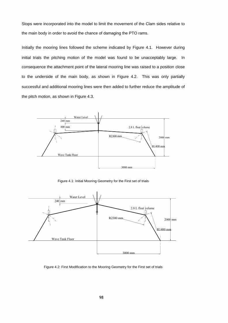
98

Stops were incorporated into the model to limit the movement of the Clam sides relative to

the main body in order to avoid the chance of damaging the PTO rams.

Initially the mooring lines followed the scheme indicated by Figure ‎4.1. However during

initial trials the pitching motion of the model was found to be unacceptably large. In

consequence the attachment point of the lateral mooring line was raised to a position close

to the underside of the main body, as shown in Figure ‎4.2. This was only partially

successful and additional mooring lines were then added to further reduce the amplitude of

the pitch motion, as shown in Figure ‎4.3.

Figure ‎4.1: Initial Mooring Geometry for the First set of trials

Figure ‎4.2: First Modification to the Mooring Geometry for the First set of trials

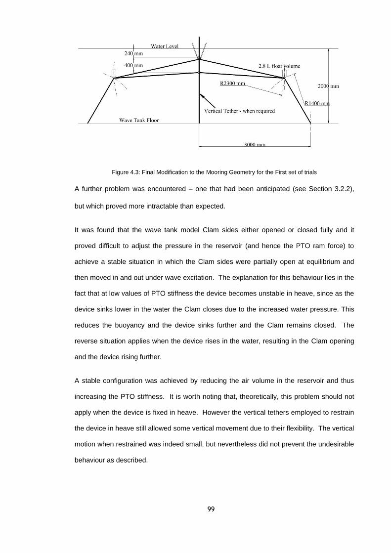
99

Figure ‎4.3: Final Modification to the Mooring Geometry for the First set of trials

A further problem was encountered – one that had been anticipated (see Section ‎3.2.2),

but which proved more intractable than expected.

It was found that the wave tank model Clam sides either opened or closed fully and it

proved difficult to adjust the pressure in the reservoir (and hence the PTO ram force) to

achieve a stable situation in which the Clam sides were partially open at equilibrium and

then moved in and out under wave excitation. The explanation for this behaviour lies in the

fact that at low values of PTO stiffness the device becomes unstable in heave, since as the

device sinks lower in the water the Clam closes due to the increased water pressure. This

reduces the buoyancy and the device sinks further and the Clam remains closed. The

reverse situation applies when the device rises in the water, resulting in the Clam opening

and the device rising further.

A stable configuration was achieved by reducing the air volume in the reservoir and thus

increasing the PTO stiffness. It is worth noting that, theoretically, this problem should not

apply when the device is fixed in heave. However the vertical tethers employed to restrain

the device in heave still allowed some vertical movement due to their flexibility. The vertical

motion when restrained was indeed small, but nevertheless did not prevent the undesirable

behaviour as described.

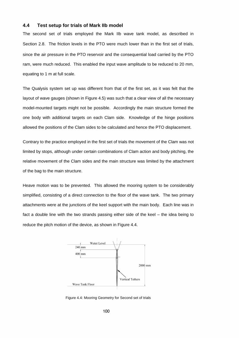
100

4.4 Test setup for trials of Mark IIb model

The second set of trials employed the Mark IIb wave tank model, as described in

Section ‎2.8. The friction levels in the PTO were much lower than in the first set of trials,

since the air pressure in the PTO reservoir and the consequential load carried by the PTO

ram, were much reduced. This enabled the input wave amplitude to be reduced to 20 mm,

equating to 1 m at full scale.

The Qualysis system set up was different from that of the first set, as it was felt that the

layout of wave gauges (shown in Figure 4.5) was such that a clear view of all the necessary

model-mounted targets might not be possible. Accordingly the main structure formed the

one body with additional targets on each Clam side. Knowledge of the hinge positions

allowed the positions of the Clam sides to be calculated and hence the PTO displacement.

Contrary to the practice employed in the first set of trials the movement of the Clam was not

limited by stops, although under certain combinations of Clam action and body pitching, the

relative movement of the Clam sides and the main structure was limited by the attachment

of the bag to the main structure.

Heave motion was to be prevented. This allowed the mooring system to be considerably

simplified, consisting of a direct connection to the floor of the wave tank. The two primary

attachments were at the junctions of the keel support with the main body. Each line was in

fact a double line with the two strands passing either side of the keel – the idea being to

reduce the pitch motion of the device, as shown in Figure ‎4.4.

Figure ‎4.4: Mooring Geometry for Second set of trials

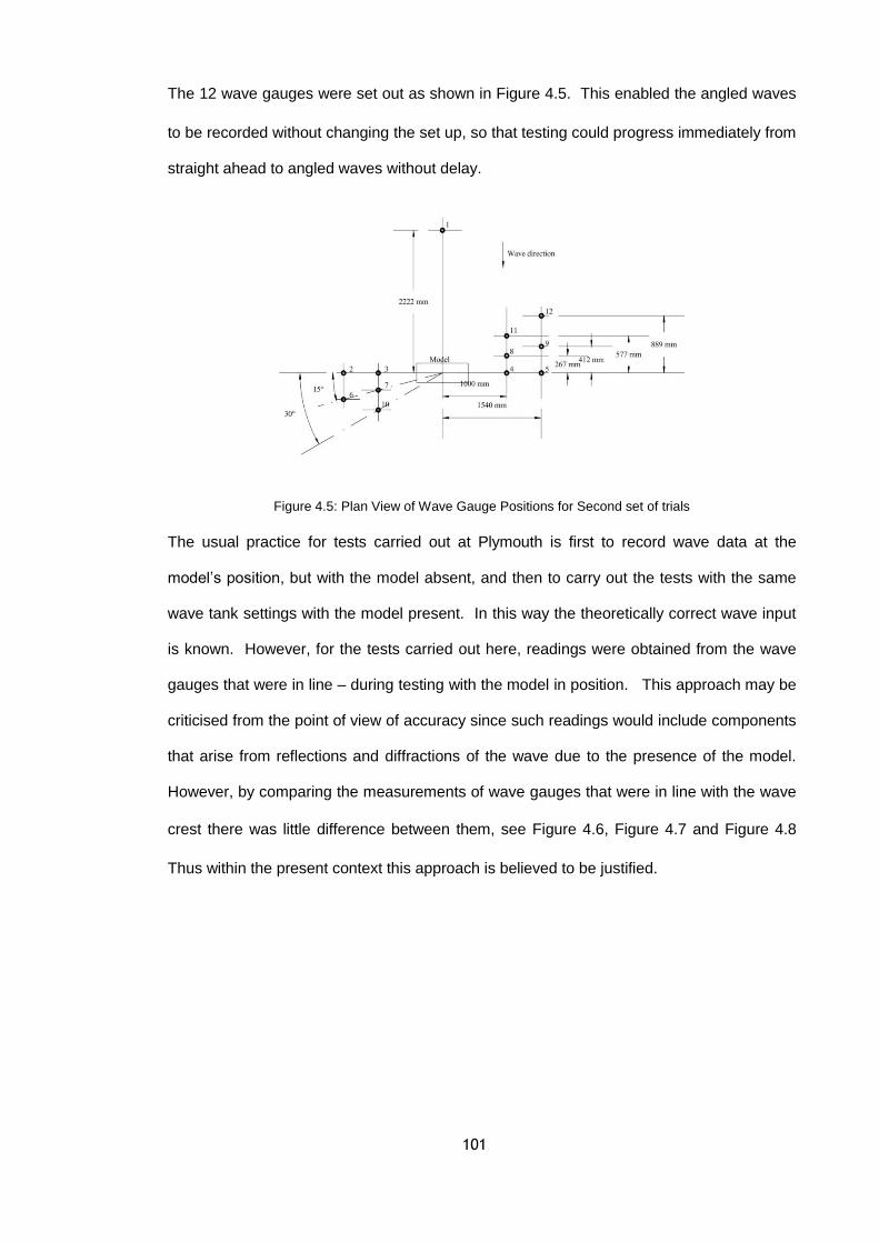
101

The 12 wave gauges were set out as shown in Figure ‎4.5. This enabled the angled waves

to be recorded without changing the set up, so that testing could progress immediately from

straight ahead to angled waves without delay.

Figure ‎4.5: Plan View of Wave Gauge Positions for Second set of trials

The usual practice for tests carried out at Plymouth is first to record wave data at the

model’s position, but with the model absent, and then to carry out the tests with the same

wave tank settings with the model present. In this way the theoretically correct wave input

is known. However, for the tests carried out here, readings were obtained from the wave

gauges that were in line – during testing with the model in position. This approach may be

criticised from the point of view of accuracy since such readings would include components

that arise from reflections and diffractions of the wave due to the presence of the model.

However, by comparing the measurements of wave gauges that were in line with the wave

crest there was little difference between them, see Figure ‎4.6, Figure ‎4.7 and Figure ‎4.8

Thus within the present context this approach is believed to be justified.

102

Figure ‎4.6: Wave gauge readings for a wave incident angle of 0° - trial 7


103


4.5 Trials programme

The trials programme was aimed at validating the theory outlined in Chapter ‎3, in order to

support the design choices and performance predictions for the full scale device described

in Chapter ‎5.

The analysis has been carried out using a number of linked applications. A standardised

spreadsheet was devised, into which the raw data from each run was input. Each trial

consisted of 8 runs as described in Section ‎4.1. A master spreadsheet then took the data

from these 8 spreadsheets in order to produce plots, such as for Power Capture, RAOs,

phase relationships etc.

Theoretical predictions were generated using the programs discussed in Chapter ‎3. The

Mathcad frequency domain model provided the hydrodynamic coefficients and other data

for input to the time domain model. This latter model then simulated the dynamic behaviour

of the device, taking into account the effect of PTO friction (see Section ‎3.11.5) in order to

provide data for comparison with the practical results.

104

The full set of trials is indicated by the two tables contained in Appendix B. A subset of

these has been selected for detailed analysis as indicated by Table ‎4.1, and has been

renumbered in a logical sequence that follows the steps taken to improve the power

capture performance of the device. Thus Trial 1 examined the behaviour of the Mark IIa

model (described in Section ‎2.7) as a floating rigid body to verify that the heave resonance

was as expected, while Trials 2 and 3 employed floating and heave restrained

configurations respectively. These latter two trials demonstrated that the device behaviour

was in line with expectations although friction in the PTO was detrimental to the power

capture performance. Trial 3 provided a practical demonstration of the benefit of restricting

heave motion.

For trials 4 to 7 the moorings were reconfigured in order to prevent heave motion, and were

carried out using the Mark IIb model as described in Section ‎2.8. Trial 4 employed coil

springs and in this configuration it proved impossible to achieve a sufficiently low value of

PTO stiffness. Nevertheless the dynamic behaviour of the model was in line with

theoretical predictions. Trials 5 through to 7 employed the constant force springs and were

able to demonstrate the performance of the device when PTO stiffness and damping

values were more in line with those suggested by theory. The results clearly show the

benefit of reducing PTO stiffness. Trial 5 used a low value of PTO damping with the aim of

demonstrating good power capture at short wave periods. Predictably the Clam amplitude

at the longer periods was excessive, limited only by the available PTO stroke. Trials 6 and

7 employed PTO stiffness and damping closer to the ideal.

The performance of the device depends on the PTO stiffness and damping as well as the

mooring geometry and internal friction. After having presented the results of the trials the

influence of these parameters on the performance of the device is discussed in ‎0.

For ease in discriminating measured data from calculated predictions, the latter are shown

by solid lines in Figure ‎4.9 through to Figure ‎4.26. Although such data is continuous,

values have been computed only at the points shown.

105

Table ‎4.1: Trials selected for detailed analysis

Appendix B trial ref D

Q

R

8

1,2

&3

15

17

to

21

Pa

ram

ete

r va

lue

s u

sed

in m

ath

em

atica

l an

aly

sis

PT

O

Fri

ctio

n

at

Mod

el

Sca

le,

N

N/A

24

12

3

6

3

2

PT

O

Fri

ctio

n a

t

Fu

ll S

ca

le,

MN

N/A

3.0

1.5

0.3

75

0.7

5

0.3

75

0.2

5

PT

O

stiffn

ess,

MN

/m

40

0

2.2

21

1.1

1

2.3

75

0.0

68

0.0

74

0.0

74

PT

O

da

mpin

g,

MN

s/m

40

1.2

68

1.6

1.0

0.1

48

1.3

95

1.8

Hea

ve

stiffn

ess,

MN

/m

0.6

0.6

20

10

,000

10

,000

10

,000

10

,000

Hea

ve

da

mpin

g,

MN

s/m

1

1.5

2

10

,000

10

,000

10

,000

10

,000

Wa

ve

Ta

nk T

ria

ls

Dam

pin

g o

rifice

dia

me

ter

N/A

3 m

m

(2 o

ff)

2.5

mm

3 m

m

5 m

m

3 m

m

2.5

mm

Descrip

tio

n

Flo

atin

g, fixe

d C

lam

an

gle

Flo

atin

g,

Fix

ed

in H

ea

ve

Fix

ed

in H

ea

ve

,

Coil

sp

ring

s

Fix

ed

in H

ea

ve

,

Con

sta

nt

forc

e s

prin

gs

Fix

ed

in H

ea

ve

,

Con

sta

nt

forc

e s

prin

gs

Fix

ed

in H

ea

ve

,

Con

sta

nt

forc

e s

prin

gs

Wa

ve

Ta

nk

Mo

del

Ma

rk IIa

Ma

rk IIa

Ma

rk IIa

Ma

rk IIb

Ma

rk IIb

Ma

rk IIb

Ma

rk IIb

Tri

al

Num

be

r

1

2

3

4

5

6

7

106

4.5.1 Trial 1 - Floating, Rigid body

For this trial the Clam mode was inhibited by replacing the PTO with a fixed length prop,

the objective being to validate the theoretical model in this simple configuration, i.e. to

determine the heave resonance and to see whether the PTO loads conformed to theory.

High values of PTO damping and stiffness (Table ‎4.1) were input to the time domain model

to effectively prevent Clam motion – even higher values resulted in model instability and

were not therefore used. The chosen values of Heave damping and stiffness provided a

match with the measured resonant peak RAO. The Response Amplification Operator, or

RAO, is the ratio of the amplitude of the output parameter, heave or PTO displacement, to

the wave input amplitude. See Equation ‎3.28 for its mathematical definition.

Figure ‎4.9 shows the comparison between predicted and measured heave response in

terms of RAO and phase lag for a wave input amplitude of 20 mm. As can be seen from

the RAO plot, the measured response is generally in line with expectations and the

resonant peak is consistent with theory. However at the longer wave periods the RAO falls

to unity faster than theory would suggest, possibly due to drag effects causing the device to

move with the motion of the waves. The measured phase lag at the longer wave periods

shows the heave motion leading the waves. At very long wave periods a floating body will

simply rise and fall with the waves, with zero phase lag. Thus the calculated values of

phase approach zero as the wave period increases, as shown by the continuous curve of

Figure ‎4.9.

The measured values of Figure ‎4.9 however, show a phase lead approaching 20° which is

difficult to explain. Two causes for this behaviour have been investigated. Firstly, and

most likely, there could have been a timing error in the wave data, due possibly to a

problem with the synchronisation signal within the data gathering system. A second cause

could be a positional effect due to the model not being in line with the wave gauges. Of

these two possibilities the first has been investigated by the laboratory staff and no fault

has been found and the second cause requires a positional error that is not seen on the

relevant video recordings. The discrepancy between measured and predicted phase is

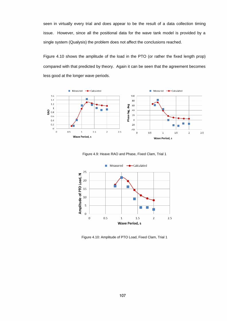
107

seen in virtually every trial and does appear to be the result of a data collection timing

issue. However, since all the positional data for the wave tank model is provided by a

single system (Qualysis) the problem does not affect the conclusions reached.

Figure ‎4.10 shows the amplitude of the load in the PTO (or rather the fixed length prop)

compared with that predicted by theory. Again it can be seen that the agreement becomes

less good at the longer wave periods.

Figure ‎4.9: Heave RAO and Phase, Fixed Clam, Trial 1

Figure ‎4.10: Amplitude of PTO Load, Fixed Clam, Trial 1

108

4.5.2 Trial 2 - Floating Clam

For this trial the Clam sides were allowed to move and the two PTOs were placed in

position. The values of PTO damping and stiffness were chosen from the point of view of

ensuring effective power capture, Table ‎4.1. Also shown is the value of Coulomb Friction,

which, being undesirably high, considerably affected the performance of the device.

Nevertheless agreement between the theoretical predictions and trial results served to

validate the analysis and provide confidence in the mathematical modelling. The wave

amplitude for this trial was 40 mm which is equivalent to 2 m at full scale. This is an

increase from the desirable amplitude of 20 mm and was necessary in order to overcome

the friction in the PTO.

In matching the calculated heave response to the observed behaviour, the heave damping

used in the time domain model was increased from that of trial 1 but the heave stiffness

was the same (see Table ‎4.1). PTO damping and stiffness were calculated from

knowledge of the characteristics of the orifice and the coil springs, while the Coulomb

Friction level in the PTO was chosen to provide a match between the calculated and

observed response of the device. Figure ‎4.11 shows the comparison between calculated

and measured heave response while Figure ‎4.12 shows the comparison between

calculated and measured PTO response. As can be seen from Figure ‎4.12 the match with

the PTO RAO is not good. However, if the heave damping and PTO friction values are

chosen in order to provide a better match with the measured PTO RAO and PTO load, then

the power capture is over-estimated.

Figure ‎4.13 shows the measured PTO load compared with calculated values and again the

match is not good. Figure ‎4.14 shows the power capture as a function of wave period, at

both model and full scales (for the same basic data).

To fully understand the behaviour of the floating device, more test and analysis work would

be needed. The mathematical model would require the inclusion of viscous drag on the

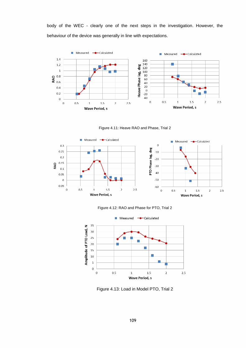
109

body of the WEC - clearly one of the next steps in the investigation. However, the

behaviour of the device was generally in line with expectations.

Figure ‎4.11: Heave RAO and Phase, Trial 2

Figure ‎4.12: RAO and Phase for PTO, Trial 2

Figure ‎4.13: Load in Model PTO, Trial 2

110

Figure ‎4.14: Power Capture, Trial 2, (a) model scale, (b) full scale

4.5.3 Trial 3 - No heave, 40 mm wave input

Trial 3 was the carried out on the final day of the first set of trials. One of the PTOs was

leaking and was therefore removed, as was one of the two coil springs. The air pressure

in the one remaining PTO air reservoirs was increased to a level necessary to keep the

Clam sides apart – and to counteract the load of the tension spring.

The device was considerably lightened in order that the heave movement could be more

effectively reduced by using the model’s buoyancy to keep the vertical tethers taut. The

total mass in this configuration was 24.3 kg, which compares with its 43 kg displacement.

The heave damping and stiffness were chosen in order to provide a match with the

observed heave response, since although the aim was to prevent heave motion this was

not entirely possible owing to the flexibility of the mooring lines. Table ‎4.1 shows the

resulting estimated values of PTO Damping, Stiffness and Coulomb Friction.

As in the earlier trials the wave amplitude was 40 mm.

Figure ‎4.15 shows the comparison between calculated and measured heave response

while Figure ‎4.16 shows the comparison between calculated and measured PTO response.

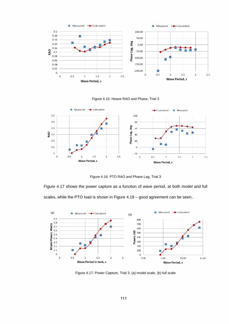
111

Figure ‎4.15: Heave RAO and Phase, Trial 3

Figure ‎4.16: PTO RAO and Phase Lag, Trial 3

Figure ‎4.17 shows the power capture as a function of wave period, at both model and full

scales, while the PTO load is shown in Figure ‎4.18 – good agreement can be seen..


112

Figure ‎4.18: Load in Model PTO, Trial 3

4.5.4 Trial 4 – No Heave, 20 mm wave input, coil spring

The configuration adopted for this trial - and the remaining trials – was the use of one PTO

assembly designed to provide the desired level of damping with the majority of the PTO

stiffness being provided by steel springs – either conventional coil springs or the special

constant force springs. As for trial 3, the device was lightened in order to provide excess

buoyancy so as to maintain the mooring lines in tension and thus restrict heave motion.

Table ‎4.1 shows the estimated values of PTO Damping, Stiffness and Coulomb Friction.

The PTO stiffness was far from ideal but was the lowest value that could be achieved from

an arrangement where the springs had to support the hydrostatic pressure on the Clam

sides and also meet the necessary stroke length.

The heave damping and stiffness chosen for mathematical modelling were such that they

effectively prevented heave. The wave amplitude was 20 mm. Figure ‎4.19 shows the

comparison between calculated and measured PTO/Clam response and PTO Load.

Figure ‎4.19: RAO, Phase Lag and Load Amplitude in Model PTO, Trial 4

113

Calculated versus measured power capture is shown in Figure ‎4.20. Here it can be seen

that the power capture is poor, as compared with the potential levels of power capture

indicated by the “½ power in 40m wave front” line. This is due to the PTO stiffness being so

far from ideal (as explained above). However there is general agreement between the

calculated and measured data.


4.5.5 Trial 5 – 20mm wave, constant force spring, 5 mm orifice

The configuration adopted for this trial used the PTO assembly that was designed to

provide the desired level of damping with the majority of the PTO stiffness being provided

by steel springs – either conventional coil springs or special constant force springs. In this

case the constant force springs were used. The device was lightened in order that its

buoyancy would maintain the mooring lines in tension and thus restrict heave motion.

At wave periods greater than 1.2 s, the PTO movement exceeded the capability of the

device. Consequently for Trial 5 the testing was restricted to wave periods between 0.6 and

1.2 seconds.

Table ‎4.1 shows the resulting estimated values of PTO Damping, Stiffness and Coulomb

Friction for trial 5. The PTO stiffness was a practical minimum and was due solely to the

114

compressibility of the air in the reservoir, while the level of PTO damping arose from the

use of a 5 mm diameter damping orifice. The wave amplitude was 20 mm.

Figure ‎4.21 shows the comparison between calculated and measured PTO/Clam response

and PTO Load. As in previous trials the PTO lag was significantly less than calculated.


that the power capture is in line with calculated levels – and is of the expected form,

including the “kink” at a model period of 1 sec. The “1/2 Power in 40m wave front” line is

added for comparative purposes; representing as it does, the best that can reasonably be

expected from the device.



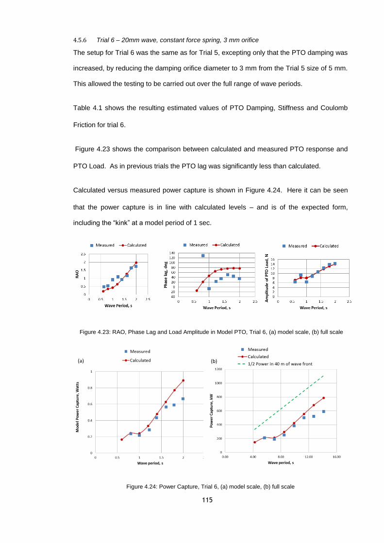
115

4.5.6 Trial 6 – 20mm wave, constant force spring, 3 mm orifice

The setup for Trial 6 was the same as for Trial 5, excepting only that the PTO damping was

increased, by reducing the damping orifice diameter to 3 mm from the Trial 5 size of 5 mm.

This allowed the testing to be carried out over the full range of wave periods.

Table ‎4.1 shows the resulting estimated values of PTO Damping, Stiffness and Coulomb

Friction for trial 6.

Figure ‎4.23 shows the comparison between calculated and measured PTO response and

PTO Load. As in previous trials the PTO lag was significantly less than calculated.


that the power capture is in line with calculated levels – and is of the expected form,

including the “kink” at a model period of 1 sec.

Figure ‎4.23: RAO, Phase Lag and Load Amplitude in Model PTO, Trial 6, (a) model scale, (b) full scale


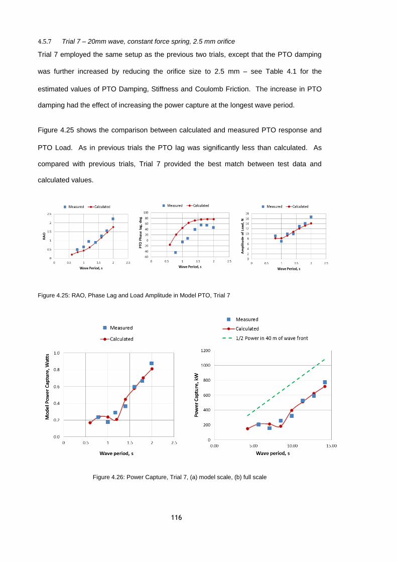
116

4.5.7 Trial 7 – 20mm wave, constant force spring, 2.5 mm orifice

Trial 7 employed the same setup as the previous two trials, except that the PTO damping

was further increased by reducing the orifice size to 2.5 mm – see Table ‎4.1 for the

estimated values of PTO Damping, Stiffness and Coulomb Friction. The increase in PTO

damping had the effect of increasing the power capture at the longest wave period.

Figure ‎4.25 shows the comparison between calculated and measured PTO response and

PTO Load. As in previous trials the PTO lag was significantly less than calculated. As

compared with previous trials, Trial 7 provided the best match between test data and

calculated values.



117

4.5.8 Variation of power capture with wave input angle

Two ad-hoc investigations were carried out, looking at the effect of varying the angle of

incidence of the incoming wave. The first involved the model configured as for Trial 5, i.e.

with the 5 mm orifice.

The angled waves were produced by appropriate changes to the wave tank control input

data files. The readings from the wave gauges confirmed that the demanded incident wave

angles and wave amplitudes had been achieved, as shown in Section ‎4.4.

The result of this investigation is shown in Figure ‎4.27, which shows a reduction in power

capture as the incident angle is increased. It should be noted that the longer wave periods

could not be investigated due to stroke limitations of the PTO.

Figure ‎4.27: Power Capture variation with wave angle; model configured as for Trial 5

118

The second set of runs was carried out with the model configured as for Trial 7, i.e. with the

2.5 mm orifice. The results are shown in

Figure ‎4.28.

Figure ‎4.28: Power Capture variation with wave angle; model configured as for Trial 7

Interestingly the device captures more power from the angled waves than those at zero

incidence, at least at the longer wave periods. The converse is true for the short period

waves.

No explanation is offered for this finding, due to both a lack of time to investigate and also

the need for a more extensive investigation, which should be one of the topics for future

work, both experimentally and theoretically. It is suggested that the present analysis

methodology is followed in the future. WAMIT, for example allows wave incidence angle to

be specified by the data input file.

119

4.5.9 Time domain modelling – Trial 7

Figure ‎4.29 shows a 4 seconds “clip” from Run 5 of Trial 7, i.e. a nominal input wave

amplitude of 20 mm and a period of 1.4 seconds. Mean removal has been applied to each

of the data series. Figure ‎4.30 shows the corresponding plots generated by the time

domain model, using an equivalent sine wave input - see Section ‎3.11.6 for the

mathematical methods employed.

Figure ‎4.29: Wave Tank Data - Trial 7, Run 5

Figure ‎4.30: Time domain model simulation - Trial 7, Run 5

As can be seen, there is good general agreement between the measured and calculated

system behaviour. In particular the calculated PTO Load plot has the same characteristic

shape as the measured data.

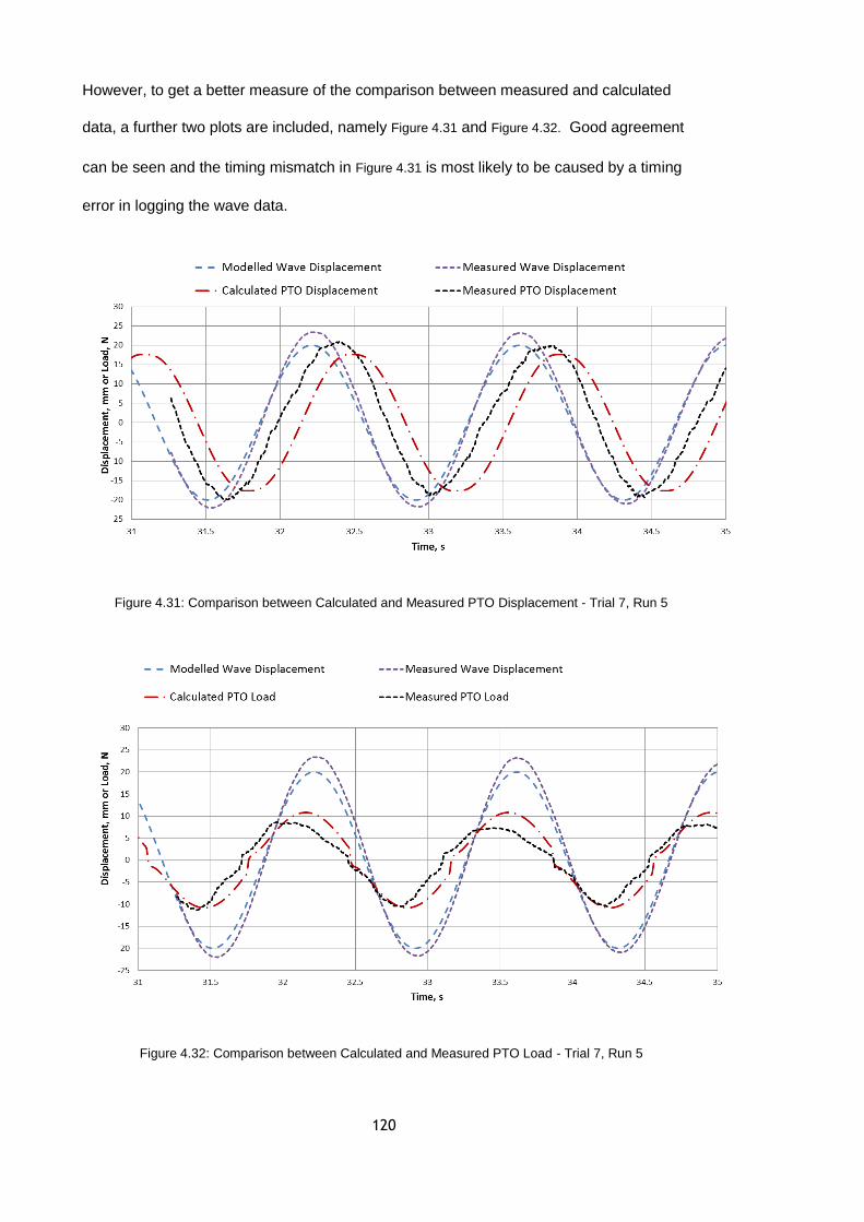
120

However, to get a better measure of the comparison between measured and calculated

data, a further two plots are included, namely Figure ‎4.31 and Figure ‎4.32. Good agreement

can be seen and the timing mismatch in Figure ‎4.31 is most likely to be caused by a timing

error in logging the wave data.

Figure ‎4.31: Comparison between Calculated and Measured PTO Displacement - Trial 7, Run 5

Figure ‎4.32: Comparison between Calculated and Measured PTO Load - Trial 7, Run 5

121

4.5.10 Performance in random seas

A test was carried out with the same physical model as for Trial 7. The angle of wave

incidence was 0° and the wave tank was programmed to deliver a Pierson-Moskowitz

spectrum with the parameters given in column 2 of Table ‎4.2. Column 3 gives the full

scale values – obtained by appropriately scaling the values in column 2 (scaling factors

listed in Appendix A). PM2 is the arbitrarily chosen name for the wave tank settings of this

test.

In order to provide confidence in the data it was decided to analyse the measured wave

data from the test using a method that included a Fast Fourier Transform function within the

Mathcad toolbox - the 4th

column of Table ‎4.2 gives the results. Figure ‎4.33 shows the

Power Spectral Density, PSDj, compared with the spectrum used in the frequency domain

analysis, Sj, with the measured value of Tz as input - see equation ‎1.11. Periodj is the

wave period in seconds, while ‘j’ is an index used in the calculation.

Comparing the column 4 data of Table ‎4.2 with that of column 3, it appears that the

parameter, Ts, used in the wave tank set up is the Zero Crossing Period, rather than the

Significant Period – the usual interpretation of the symbol, Ts.

Figure ‎4.33: Measured PSD for Trial 20 compared with smooth spectrum used for analysis

m2s

sec 0 5 10 150

5

10

15

20

Sj

PSDj

Periodj

122

Table ‎4.2: Random Sea, PM2

Parameter Value at model scale

Full scale value Measured value (full scale)

Significant Height, Hs 48 mm 2.4 m 2.505 m

Hsig 89 mm 4.45 m ----

Max Amplitude 79 mm 3.95 m 2.46 m

Peak Frequency 0.9 Hz 6.36 s ----

Equivalent Peak Period

1.111 s 7.857 s ----

Ts 0.920 s 6.505 s ----

Energy Period, Te ---- ---- 8.206 s

Zero Crossing Period, Tz

---- ---- 6.911 s

Figure ‎4.34 shows a 6 seconds “clip” from Trial 20. Mean removal has been applied to

each of the data series.

Figure ‎4.35 shows the corresponding plots generated by the time domain model, using the

measured wave data as input - see Section ‎3.11.6 for the mathematical methods

employed.

As can be seen, there is good general agreement between the measured and calculated

system behaviour. In particular the calculated PTO Load plot has the same characteristic

shape as the measured data. Also it can be seen that in common with every trial, the PTO

Position and Load plots show a measured lag that is less than that indicated by the

calculated data.

The hydrodynamic data chosen for the mathematical modelling was that appropriate to the

computed energy period of 8.206 seconds. It was found that this provided the best match

with the measured data in respect of the magnitude of the system responses.

The measured mean power capture was 233 kW when scaled to full size, while the

comparable time domain model produced a figure of 232 kW.

123

Figure ‎4.34: Wave Tank Data – Random Seas, PM2

Figure ‎4.35: Time domain model simulation - Random Seas, PM2

As in the case of the regular wave data, a further two plots are included, namely

Figure ‎4.36 and Figure ‎4.37. Good agreement can be seen and the timing mismatch can

again be detected.

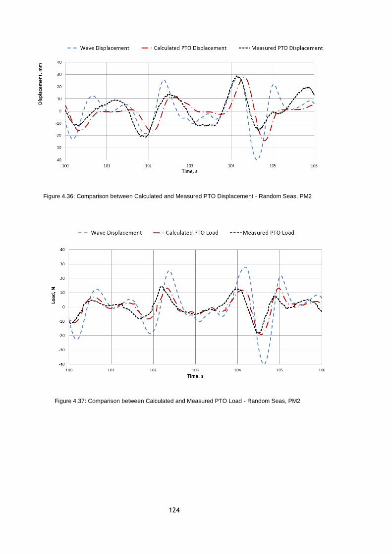
124

Figure ‎4.36: Comparison between Calculated and Measured PTO Displacement - Random Seas, PM2

Figure ‎4.37: Comparison between Calculated and Measured PTO Load - Random Seas, PM2

125

A further check on the validity of the mathematical modelling was carried out. This entailed

using Mathcad to calculate the power capture using the Pierson-Moskowitz spectrum (see

Section ‎3.10 for method) and comparing it with the value calculated by the time domain

model using the measured values of Significant Wave Height, Hs, and Energy Period, Te

given in Table ‎4.2 as input. In order to make the comparison, the Coulomb friction in the

time domain model was set to zero since the frequency domain model had no provision to

allow for friction. The resulting figures were:

From frequency domain model: 301 kW

From time domain model simulation: 283 kW

These figures do not show total agreement, but are within 10% of each other which

demonstrates the validity of the mathematical modelling. In the future it is hoped to adopt a

more mathematically correct method of analysis using a convolution integral approach; and

this would naturally be expected to produce a more accurate prediction. However the

approximate approach can be seen to give acceptably close results for the purpose of

hardware and control system design. With a Coulomb friction value of 2 N (model scale)

the time domain model predicted a power capture of 232kW – as reported above.

4.5.11 Performance in random seas with spread

As a final test of the performance of the Clam, model was tested with the same

specification of wave spectrum as previously – but with a spreading factor of 12. This is the

spreading factor that would be appropriate for summer conditions at Wave Hub (Daruvala,

2009). The measured power capture was 198 kW as compared with nominally the same

wave input but without spread, of 233 kW – a reduction of 15%.

126

4.6 Discussion of trial results

The aim of the practical testing was to examine the performance across a wide range of

operating conditions, rather than looking at just one or two conditions in depth. This aim

has been achieved, in that all the plotted curves display a behaviour that compares well

with theory – to the extent that the shape of the curves is similar.

In examining the data and the modelling predictions certain questions naturally arise:

Why does the power capture performance curve display a “kink”?

Why does the power capture performance curve tend to naturally follow the curve

of available wave power across a wide range of wave periods?

What are the main drivers in determining power capture performance?

What level of confidence can be put on the performance predictions?

How does the performance of this device compare with other wave energy

converters?

These questions provide the headings that follow:

Why does the power capture performance curve display a “kink”?

Referring to the performance data for trial 7 as shown in Figure ‎4.26, a local minimum in

power capture occurs at a wave period of around 8.5 seconds. This characteristic is seen

in both the measured and calculated data. The obvious answer to the question is that the

hydrodynamic and other physical characteristics of the system are such as to produce this

result – and that the mathematical modelling of the system is correct. The hydrodynamic

coefficients have been examined in the hope that a simple explanation for the shape of the

performance curve might be found. However, there seems to be no single piece of data

that provides an explanation and this is a question that could be examined more fully in the

future.

127

Why does the power capture performance curve tend to naturally follow the curve of

available wave power across a wide range of wave periods?

The conventional wisdom regarding the mechanism of WEC maximum power capture may

be captured by the following two statements (Shaw, 1982):

1) The undamped natural frequency should be matched to the forcing frequency of the

waves, and

2) The energy extraction damping coefficients should be equal to the sum of the

hydrodynamic damping coefficients and viscous damping coefficients due to the

motion of the WEC.

In the case of the present device the only mode of interest is mode 7, the Clam or PTO

mode. Natural frequency is related to mass and stiffness values, Section ‎1.5.2 and

equation ‎1.26.

The only movement is that of the Clam sides, and these have negligible mass in relation to

the surrounding water. Thus the undamped natural frequency and hence resonant period

depend on the hydrodynamic and hydrostatic coefficients alone, as in equation ‎4.1:

𝜔0 = √

𝐶77

𝐴77 and thus 𝑇0 =

2𝜋

𝜔0

(‎4.1)

where 𝐶77 is the Clam Hydrostatic Coefficient and 𝐴77 is the Clam Added Mass, 𝜔0 is the

undamped radian frequency and 𝑇0 is the undamped resonant period.

128

Figure ‎4.38 shows the comparison of the undamped resonant period, calculated using

equation ‎4.1 with the ideal situation of equalling the input wave period. Thus between, say,

a 5 s and 13 s period the resonant period of the system provides a reasonable match with

the wave input.

Figure ‎4.38: Resonant Period of Clam mode

The second requirement for maximum power capture is that the energy extraction damping

coefficients should be equal to the sum of the hydrodynamic damping coefficients and

viscous damping coefficients due to the motion of the WEC.

The hydrodynamic damping coefficient, 𝐵77, has the value of 0.0318 MNs/m for a 10 s

wave, which is much less than the 1.8 MNs/m for PTO damping that has been found during

the practical testing to be a good value to use, (Table ‎4.1)

If the PTO damping is given the values in the region of 0.03 MNs/m to 0.04 MNs/m, in line

with conventional wisdom, the result is good power capture at the resonant period, as

would be expected, but much poorer power capture at other wave periods. Also the PTO

RAOs are unrealistically large, since the available stroke of the PTO would not be

sufficient. It is likely that the increased stroke (if achieved) would result in increased viscous

drag, and a consequent reduction in power capture.

Thus the key to the wide band response would appear to lie in the natural ability of the

Clam resonance to match the input wave period.

Wave Period, s

Clam Resonant Period, s

129

What are the main drivers in determining power capture performance?

As has been seen from the test programme and modelling studies reported here, heave

damping and stiffness have a marked effect on power capture. Also it appears necessary

to prevent heave motion as much as possible. Both practical testing and mathematical

modelling indicate that the PTO stiffness should be as low a value as possible. PTO

Damping should be chosen on the basis of mathematical modelling simulations. In

addition, friction within the WEC should be kept as low as possible. This may be

demonstrated by reference to the setup for Trials 6 and 7.

Rows 1 and 4 of Table ‎4.3 contain the values of friction, stiffness and damping that were

considered appropriate for trials 6 and 7, respectively. The resulting calculated power and

PTO RAO is also shown, as is the measured power. In the case of trial 6, the comparison

between calculated and measured power is not good. In examining the trial data and

spreadsheet calculations the explanation for the discrepancy would appear to lie in the fact

that the pressure in the air reservoir in trial 6 was too low for this particular wave period,

with the consequence that the PTO ram did not remain in sufficiently good contact with the

Clam sides throughout the cycle.

Rows 2, 3, 5 and 6 of Table ‎4.3, show the effect of reducing friction and PTO stiffness

whilst maintaining the PTO RAO to a value of 2 or less. To achieve this aim, the PTO

damping value of row 3 has been increased from the row 2 value. If however the limitation

on PTO RAO is ignored the power capture can be significantly increased, as shown by the

data in row 7. In this case the all the available wave power over the 40 m width of the Clam

is captured. In practice this would not be possible due to the design limitations on PTO

stroke and also the effect of viscous drag that would accompany the increased movement

of the Clam sides. However, it is instructive to examine the effect of allowing an increase in

PTO stroke and Table ‎4.4 shows the result of a brief investigation. In this case the PTO

damping figure was retained at 0.23 MNs/m and the friction level was increased. Since the

friction in the wave tank model is measured by the load cells and contributes to the power

130

capture measurement, the mathematical model does the same. Hence this strategy is

equivalent to employing Coulomb damping in the PTO.

Table ‎4.3: Effect of PTO stiffness, damping and friction on performance of Clam at 12.73 s period

Ro

w

Tri

al

Fri

cti

on

, M

N

PT

O

Sti

ffn

es

s,

MN

/m

PT

O

Da

mp

ing

,

MN

s/m

Ca

lcu

late

d

Po

we

r, k

W

Me

asu

red

Po

we

r, k

W

Ca

lcu

late

d

Cla

m/P

TO

RA

O

Ca

lcu

late

d

Ca

ptu

re

Wid

th,

m

1 6 0.375 0.074 1.395 689.5 563 1.624 14.2

2 -- 0.0 0.074 1.395 884 --- 2.28 18.2

3 -- 0.0 0.0 1.6 810 --- 2.038 16.6

4 7 0.250 0.074 1.8 621 615 1.468 12.8

5 -- 0.0 0.074 1.8 732 --- 1.83 15.0

6 0.0 0.0 1.8 740 --- 1.84 15.2

7 -- 0.0 0.0 0.23 1932 --- 8.303 39.7

Table ‎4.4: Effect on power capture of increasing Clam RAO - at 12.73 s wave period

Friction, MN

PTO Stiffness,

MN/m

PTO Damping,

MNs/m

Calculated Power, kW

Calculated Clam/PTO

RAO

Calculated Capture Width, m

0.0 0.0 0.23 1932 8.303 39.7

0.3 0.0 0.23 1839 6.56 37.8

0.6 0.0 0.23 1587 4.81 32.6

0.8 0.0 0.23 1332 3.57 27.4

1.0 0.0 0.23 1016 2.51 20.9

1.083 0.0 0.23 910 2.194 18.7

1.125 0.0 0.23 804 1.89 16.5

1.2 0.0 0.23 677 1.54 13.9

Figure ‎4.39 takes values from Table ‎4.4 to show the relationship between capture width

and PTO RAO. By doubling the possible RAO from 2 to 4, the power capture is almost

doubled. Thus increasing the allowable PTO stroke should be a design aim.

131

Figure ‎4.39: Capture width versus PTO RAO

What level of confidence can be put on the performance predictions?

It is difficult to answer this question. However, it is not unreasonable to claim that the

behaviour of the device in both free floating and heave restrained configurations can be

predicted with confidence. The predictions are better and more consistent at the longer

wave periods and higher levels of power capture, say above 8 s and 450 kW.

As experience was gained in carrying out the trials, the agreement between predictions and

tests improved – as evidenced by the trial 7 results shown in Section ‎4.5.7. Figure ‎4.40

compares the measured power capture with the calculated power, and with a ± 10% band

around it. Thus using trial 7 as the standard it is reasonable to claim an accuracy of

predictions within 10% for wave periods greater than 10 s. For periods less than 10 s the

correlation is not as good.

132

Figure ‎4.40: Power prediction accuracy

Bearing in mind that these predictions are based on tests in the wave tank, it is worth

considering how the performance of a full sized device might compare. Although the

calculated predictions ignore viscosity, it would have influenced the practical results of the

wave tank testing. Viscous effects do not scale in the same way as the hydrodynamic and

inertia loads, so that at full scale they are much less significant. Accordingly the power

capture at full size is likely to be greater than the tests suggest.

133

How does the performance of this device compare with other wave energy converters?

To answer this question fully is a research project in itself. However, it is instructive to look

at a couple of examples that provide a comparison with the Clam, i.e. SPERBOYTM

and

Oyster.

Figure ‎4.41: Comparison of Clam’s Performance with Floating Oscillating Water Column WEC

Figure ‎4.41 shows the comparison of the Clam with the SPERBOYTM

floating Oscillating

Water Column (OWC) wave energy converter (Tucker et al., 2010). The power capture

data is based on a regular wave input of 1 m amplitude across the range of wave periods

shown.

The SPERBOYTM

WEC is a Point Absorber designed to operate in the highly energetic

wave climate found in the Outer Hebrides where the annual average wave power is of the

order of 62 kW per metre of wave front. The chosen location for the study was Benbecula

in the Outer Hebrides taken as the WERATLAS (INETI, 2009) data for point Barra.

Figure ‎4.42 describes the location by means of an Annual Average Spectrum that is

defined from the individual spectra for a number of wave states weighted by their frequency

of occurrence. It can be seen by comparing Figure ‎4.41 and Figure ‎4.42 that the

134

SPERBOYTM

WEC has been designed to match the characteristics of the wave resource

(Phillips & Rainey, 2005).

Figure ‎4.42: "Annual Average" Wave Input Spectrum at Benbecula (Phillips & Rainey, 2005)

The mean annual power capture of SPERBOYTM

was calculated, and confirmed by testing,

to be 700 kW – prior to considering losses in the PTO. The rating of the PTO maximum

power capture was 3 MW. However, to achieve this level of power capture the device had

the following characteristics:

Overall diameter – 40 m

Column internal diameter – 22 m

Column length (below waterline) – 70 m

Overall Mass, including ballast – 17,200 tonnes

Although a point absorber can achieve a capture width much larger than its physical size,

the range of wave periods where this applies may be small. It was found that the large size

of SPERBOYTM

was necessary to achieve a sufficiently large bandwidth.

To match the performance of SPERBOYTM

with a Clam-type WEC in the wave climate of

Benbecula, it would be necessary to increase its physical size – a not impossible task.

However, the advantage that the Clam displays lies in its performance in less energetic

locations and hence shorter wave periods.

135

A device more akin to the Clam is the Oyster WEC – a nearshore oscillating wave surge

converter that takes the form of a flap mounted on the sea floor and hinged at its base. The

Clam has a number of features in common with Oyster. In particular its physical size is

similar - as is its annual power capture, i.e. 200 kW mean power in a wave climate of 19

kW/m, although this relates to Oyster 1 which has a width of 18 m.

Oyster does not follow the conventional wisdom of Section ‎1.5.2 – it “couples with incoming

waves without being highly tuned” (Whittaker et al., 2007) and aims to optimise the wave

torque. In common with Oyster, the Clam does not follow conventional wisdom, but there

are differences. Oyster is not highly tuned whereas the Clam achieves tuning naturally, as

shown by Figure ‎4.38. At a width of 26 m Oyster 2 operates partly as a point absorber,

while studies of a wider device of 50 m width show a power capture of 50% of the incoming

wave power, which is in line with Clam experience.

Oyster’s energy capture varies with incoming wave direction. Thus the reduction in power

capture is approximately proportional to the cosine of the angle of incidence to the power of

2.1 (i.e. roughly “power squared”), such that at 90 degrees to the normal wave direction the

energy capture is zero (Whittaker et al., 2007). It is possible that the Clam performs better

than Oyster in this respect - see Figure ‎4.28 which shows little reduction in power capture,

at least up to an angle of incidence of 30°.

136

5 Full Scale Design

5.1 Introduction

Having completed the programme of analysis and experimentation it may be concluded

that the Clam-type wave energy converter (WEC) has good potential. A promising

performance regime, that of low or negative PTO stiffness, has been identified,

However, there is a not-inconsiderable amount of work needed to prove the feasibility of

the concept at full scale. In the sections that follow a possible way forward is described

and the power capture at the Wave Hub test site is estimated.

5.2 Main Features of the proposed design concept

Having demonstrated that this Clam-type wave energy converter (WEC) has potential, the

question is whether a full scale realization is feasible – one that embodies the features that

have been shown to be effective through mathematical modelling and physical model

testing.

________________________________________________________________________

The remainder of this section, which contained details of a possible full scale device, has

been removed due to Copyright restrictions.

________________________________________________________________________

5.3 Performance prediction

An assessment of the performance of a full size device at the Wave Hub test site has been

carried out using data on the annual wave climate, including directionality. The approach

that has been adopted is first to assess the device performance for a specific number of

wave states and then to curve fit these so that the annual energy capture for any desired

wave state can be found by interpolation. With knowledge of the frequency of occurrence

of each wave state the annual energy capture (and hence annual mean power capture)

may be found by summing the energy capture contribution from each wave state.

A Prototype device would have the facility to change the PTO characteristics in accordance

with whatever control philosophy is found to be appropriate. However, for the purpose of

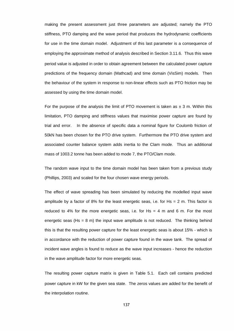
137

making the present assessment just three parameters are adjusted; namely the PTO

stiffness, PTO damping and the wave period that produces the hydrodynamic coefficients

for use in the time domain model. Adjustment of this last parameter is a consequence of

employing the approximate method of analysis described in Section ‎3.11.6. Thus this wave

period value is adjusted in order to obtain agreement between the calculated power capture

predictions of the frequency domain (Mathcad) and time domain (VisSim) models. Then

the behaviour of the system in response to non-linear effects such as PTO friction may be

assessed by using the time domain model.

For the purpose of the analysis the limit of PTO movement is taken as ± 3 m. Within this

limitation, PTO damping and stiffness values that maximise power capture are found by

trial and error. In the absence of specific data a nominal figure for Coulomb friction of

50kN has been chosen for the PTO drive system. Furthermore the PTO drive system and

associated counter balance system adds inertia to the Clam mode. Thus an additional

mass of 1003.2 tonne has been added to mode 7, the PTO/Clam mode.

The random wave input to the time domain model has been taken from a previous study

(Phillips, 2003) and scaled for the four chosen wave energy periods.

The effect of wave spreading has been simulated by reducing the modelled input wave

amplitude by a factor of 8% for the least energetic seas, i.e. for Hs = 2 m. This factor is

reduced to 4% for the more energetic seas, i.e. for Hs = 4 m and 6 m. For the most

energetic seas (Hs = 8 m) the input wave amplitude is not reduced. The thinking behind

this is that the resulting power capture for the least energetic seas is about 15% - which is

in accordance with the reduction of power capture found in the wave tank. The spread of

incident wave angles is found to reduce as the wave input increases - hence the reduction

in the wave amplitude factor for more energetic seas.

The resulting power capture matrix is given in Table ‎5.1. Each cell contains predicted

power capture in kW for the given sea state. The zeros values are added for the benefit of

the interpolation routine.

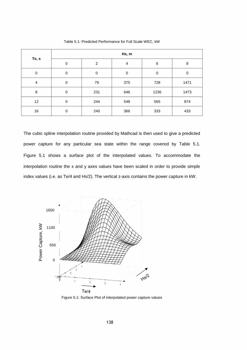
138

Po

we

r C

ap

ture

, kW

550

1650

1100

0

Table ‎5.1: Predicted Performance for Full Scale WEC, kW

Te, s

Hs, m

0 2 4 6 8

0 0 0 0 0 0

4 0 79 375 728 1471

8 0 231 646 1236 1473

12 0 244 548 565 874

16 0 240 366 333 433

The cubic spline interpolation routine provided by Mathcad is then used to give a predicted

power capture for any particular sea state within the range covered by Table ‎5.1.

Figure ‎5.1 shows a surface plot of the interpolated values. To accommodate the

interpolation routine the x and y axes values have been scaled in order to provide simple

index values (i.e. as Te/4 and Hs/2). The vertical z-axis contains the power capture in kW.

Figure ‎5.1: Surface Plot of interpolated power capture values

139

Figure ‎5.2: Joint probabilities, Hm0 (Hs) and Tm-1,0 (Te) at Wave Hub, locn 1 (Nieuwkoop et al.), 2013)

Figure ‎5.3, Mean Wave Pwr (kW/m) binned by wave dirn (°N) at Wave Hub (Nieuwkoop et al.), 2013)

Figure ‎5.2 shows the joint probability for Significant Wave Height, 𝐻𝑠 ( = 𝐻𝑚0) and Energy

Period, 𝑇𝑒 (= 𝑇𝑚−1,0) at location 1. Each square shows probability of occurrence of the

particular wave state as a percentage. Where a square shows a figure of zero the

probability of that wave state is less than 0.04%. Thus combining this data with the power

capture data of Figure ‎5.1 provides an estimate of the mean annual power capture, as in

the spreadsheet of Appendix C. The effect of wave direction is approximated by applying a

140

factor of 0.7 to wave states with energies below 24 kW/m – based on the data given in

Figure ‎5.3 (Nieuwkoop et al., 2013).

Thus, as can be seen from Appendix C, the mean annual power capture is estimated to be

179.5 kW at Wave Hub location 1, where the available annual wave power is calculated to

be 18 kW per metre of wave front. The mean annual wave power incident on the 40 m

width of the Clam is thus 700 kW, and a reasonable aim for the WEC would be half of this

figure, i.e. 350 kW. The estimate of 179.5 kW is just 51% of 350 kW. Naturally the

conversion efficiency of the generator needs to be taken into account, but bearing in mind

that the generator is directly driven by the motion of the Clam, an efficiency of 90% or

greater is not unreasonable. Thus a reasonable estimate of mean annual power capture in

a far from energetic 18 kw/m sea is 157.5 kW, wave to wire.

However there is scope for improving power capture by a suitable choice of control

methodology – and by design changes to increase the PTO stroke. In a random sea many

of the individual waves cause a PTO motion that is well within the stroke limitations, while

other waves result in PTO motion that would exceed the stroke limitation if the control

system were not designed to prevent this. A possible way forward is to design the control

system to make full use of the available stroke whatever the size of the individual waves.

The key to maximising power capture lies in the way the WEC responds to the wave action,

both in a general sense and also on a wave by wave basis. It is believed that the proposed

PTO will enable this to be done. By way of explanation consider a regular (sine wave)

input. The optimum value of PTO damping depends on the wave period. Thus at each

instant in time the force by which the PTO resists the loads put upon it, will vary according

to the desired level of damping. Thus a passive method of damping, such as that

employed by the wave tank model, is simulated by an active system that can respond to

wave period. In random waves the situation is more complex and although the damping

may be varied along the lines discussed there is the potential to implement more efficient

control strategies – a subject for further research.

141

6 Conclusions and Suggestions for further

research

6.1 Aim of the research

At the start of the project the research aim was to investigate the mechanism of power

capture from sea waves and to optimise the performance of a vee-shaped floating Wave

Energy Converter, the Floating Clam, patented by Francis Farley (Farley, 2011d). His

patent was based on the use of a pressurised bag (or ‘reservoir’) to hold the hinged Clam

sides apart, so that as they moved under the action of sae waves, air would be pumped

into and out of a further air reservoir via a turbine/generator set in order to extract power

from the system. A novel feature of the concept was the lengthening of the resonant period

in heave resulting from the flexibility of the air bag support of the Clam sides. This was

expected to lead to a reduction in the mass (and hence cost) of the Clam as compared with

a rigid body.

Further aims were to examine alternative power take-off (PTO) mechanisms and to

estimate the cost of energy produced at a sample location, such as Wave Hub.

The theoretical investigations were to be supported by the construction and testing of

suitable wave tank models.

6.2 Conclusions reached

The research supports the conclusion that the Clam is a feasible device, with development

potential. However, the most promising mode of operation is not as originally proposed,

since the Clam captures more energy when restrained in heave than when free to move in

all axes. Furthermore, practical testing confirmed by mathematical modelling, has led to

the conclusion that very low values of PTO flexibility are necessary and this in turn led to

the use of constant-force springs in the wave tank model and the pulley plus

counterbalance proposal for the full scale device. By good fortune the pulley can be

configured to provide a direct drive to the generator, thus enabling an efficient drive with

inherently very low friction losses.

142

In the time available, and due overcoming technical challenges along the way, it has not

been possible to complete the research with an estimate of the cost of energy produced.

However, a number of achievements may be claimed, and briefly summarised. In respect

of the mathematical modelling, the hydrodynamic coefficients have been curve-fitted so that

the correct values are available for any particular wave period, and the frequency domain

and time domain models are linked in such a way as to automatically use the same

hydrodynamic and hydrostatic data. Furthermore, an approximate, but most effective

method has been conceived for simulating the behaviour of the Clam in irregular waves,

which could be of great use in future control system studies, if speed of computation is an

issue. A comprehensive series of wave tank trials has been completed, and included in

this achievement is the modification of the wave tank model to achieve very low values of

PTO flexibility with negligible mechanical friction in the hinge mechanism. The novel

arrangement of wave gauges to facilitate trials of varying incident wave angles can also be

regarded as a success.

The wave tank model has demonstrated its robustness and therefore its suitability for use

in further test programmes. In particular, it should be possible to embody the design

concepts laid out in Chapter ‎5 directly into the model.

Two problems remain unresolved. The first concerns the discrepancy between calculated

and measured phase angles (Section ‎4.5.1) and the second concerns the calculation of

hydrostatic coefficients (see Section ‎3.4). The phase angle discrepancy points to a more-

or-less constant timing error of 0.15 s across all wave periods - indicating an

instrumentation problem. However, this is a preliminary finding and should be further

investigated. The calculation of hydrostatic coefficients question is unlikely to be resolved –

at least in terms of hunting down an error in the commercially supplied software.

Fortunately the error does not affect the analysis of the heave-restrained configuration.

In conclusion, at the current stage of research, the mean annual power capture is

estimated as 157.5 kW, wave to wire in a far from energetic 18 kw/m mean annual wave

climate, but with scope for improvement, including through control system development.

143

6.3 Suggestions for further research and development

A number of possible topics for study are discussed below. Some topics lie clearly in the

academic arena while others, such as the design and costing studies, would involve a

commercial input.

Mathematical modelling in the time domain should be improved through the use of

‘convolution’ in order to provide a more reliable prediction of WEC behaviour in irregular

seas. The modelling should include the PTO control system and non-linear effects, such

as friction, with allowance for skin friction and other body drag effects. The mathematical

models would include simulation of the control system and the control system real world

inputs. In fact the Clam lends itself to both theoretical and practical studies of a range of

control philosophies including reactive and latching control (see Section ‎1.5.4). The

theoretical methods and tools which have been used in the present work could be applied

to such a study, albeit with the updates just described. Practical work could be based on

further use of the wave tank model to confirm the theoretical analysis. The model PTO

could take the form of a capstan drive and stepper motor, such that with a suitable

electronic control system all possible control philosophies could be tested.

Investigations into the effect of changes to basic geometrical parameters, such as overall

size, width and clam angle should be carried out. Knowledge of the effect of such changes

on energy capture would then provide data to assist in matching the device to specific wave

climates. In order to make a more definitive prediction of energy capture in real seas a

detailed knowledge of the real sea spectra at locations of interest, such as at Wave Hub

would be needed. Where assessments are supported by physical model testing, it would

be necessary to reproduce these spectra in the wave tank. Employing standard spectra,

such a Pierson-Moskowitz is unlikely to be sufficient. The performance of the Clam when

deployed in an array should also be investigated.

A design study of the full sized WEC is clearly a necessary part of the process of estimating

the cost of generated electricity. Certain aspects of the design require more attention than

others, such as the flexible membrane, the capstan drive and the hinge. However,

144

although employing less innovative technology, the structure, the electrical machine and

associated control systems, all present significant design challenges. Integral with this

activity would be a survival assessment, with particular emphasis on the device behaviour

in very large waves. Having chosen the site and settled on a suitable design for the Clam;

the cost of manufacture, deployment, maintenance and decommissioning could be

estimated. These costs, together with knowledge of the design life, annual energy capture,

electricity distribution costs and the interest costs of financing the project, need to be taken

into account when calculating the cost of generated electricity.

145

References AeroHydro (2012) MultiSurf. [Online] Available at:

http://www.aerohydro.com/products/marine/multisurf.htm.

Anon (2016) Wave Energy Prize. [Online] Available at: http://waveenergyprize.org/teams.

AWS (2012) AWS Ocean Energy. [Online] Available at: http://www.awsocean.com.

Babarit A and Clément AH (2005) Optimal Latching Control of a Wave Energy Converter. In: 6th

European Wave and Tidal Energy Conference. Glasgow, UK. 19–26.

Barber NF and Ghey G (1969) Water Waves. London: Wykeham Publications

Bawden T (2015) Wind Power now UK’s chapest source of electricity. [Online] Available at:

http://www.independent.co.uk/environment/wind-power-now-the-cheapest-source-of-

electricity-but-the-government-continues-to-resist-onshore-a6685326.html.

Bellamy NW (1985) The Circular Sea Clam Wave Energy Converter. Coventry, England

Cahill B and Lewis AW (2014) Wave period ratios and the calculation of wave power. The 2nd

Marine Energy Technology Symposium, 1–10.

Cahill BG and Lewis AW (2011) Wave Energy Resource Characterization of the Atlantic Marine

Energy Test Site. In: 9th European Wave and Tidal Energy Conferenceth. Southampton,

UK. 1–8.

Carbon Trust (2011) Accelerating Marine Energy. Current. 103 (July), 1–64. Available at:

http://www.carbontrust.co.uk/emerging-technologies/current-focus-areas/marine-energy-

accelerator/pages/default.aspx.

Carbon Trust (2016) Carbon Trust Marine Renewables Proving Fund. [Online] Available at:

https://www.carbontrust.com/client-services/technology/innovation/marine-renewables-

proving-fund/ (accessed 12/04/16).

Carbon Trust (2006) Future Marine Energy. Development, 36. Available at:

http://www.carbontrust.co.uk/Publications/pages/PublicationDetail.aspx?id=CTC601.

Chaplin JR, Heller V, Farley FJM, Hearn GE and Rainey RCT (2012) Laboratory testing the

Anaconda. Philosophical transactions. Series A, Mathematical, physical, and engineering

sciences. 370 (1959), 403–24. Available at:

http://www.ncbi.nlm.nih.gov/pubmed/22184668 (accessed 01/09/12).

Cornett AM (2008) A global wave energy resource assessment J. S. Chung ed. Renewable

Energy. 1 (6), 1–9.

146

Craik ADD (2005) George Gabriel Stokes on Water Wave Theory. Annual Review of Fluid

Mechanics. 37 (1), 23–42. Available at:

http://www.annualreviews.org/doi/abs/10.1146/annurev.fluid.37.061903.175836 (accessed

13/03/12).

Daruvala J (2009) Sw Wave Hub - Metocean Design Basis. Liphook, Hants, UK Available at:

www.metoc.co.uk.

Dawson JK (1979) Wave Energy, Energy Paper No 42. HMSO.

Dean RG and Dalrymple RA (1991) Water Wave Mechanics for Engineers and Scientists. World

Scientific Publishing Co. Pte. Ltd

DoE UK (1985) Wave Energy : the Department of Energy’s R & D programme 1974-1983:

ETSU report; R26. ETSU for the Department of Energy

Falcão AF de O (2005) Modelling and Control of Oscillating-Body Wave Energy Converters with

Hydraulic Power Take-Off and Gas Accumulator. In: 6th European Wave and Tidal Energy

Conference. Glasgow UK. 113–120.

Falcão AF de O (2007) Phase control through load control of oscillating-body wave energy

converters with hydraulic PTO system. In: 7th European Wave and Tidal Energy

Conference. Porto, Portugal. 1–10.

Falnes J (2002) Ocean waves and oscillating systems: linear interactions including wave-energy

extraction. Cambridge: Cambridge University Press

Falnes J (2005) Principles for capture of energy from ocean waves. Phase control and optimum

oscillation. Norway

Farley FJM (2010) A new wave energy converter - the distensible buoy. Le Bar-sur-Loup

Farley FJM (2011a) clamsim8a - Excel Spreadsheet.

Farley FJM (2012) Opening remarks and the power spectrum of ocean waves. In: Philosophical

transactions. Series A, Mathematical, physical, and engineering sciences. 203–7.

Available at: http://www.ncbi.nlm.nih.gov/pubmed/22184658 (accessed 21/07/12).

Farley FJM (2011b) The conical free-floating clam. Southampton, UK

Farley FJM (2011c) The free floating clam. Southampton, UK

Farley FJM (2011d) The free floating clam - a new wave energy converter. In: 9th European

Wave and Tidal Energy Conference. Southampton, UK. 1–4.

147

Farley FJM, Rainey RCT and Chaplin JR (2012) Rubber tubes in the sea. Philosophical

transactions. Series A, Mathematical, physical, and engineering sciences. 370 (1959),

381–402. Available at: http://www.ncbi.nlm.nih.gov/pubmed/22184667 (accessed

07/09/12).

Filianoti, P U of RC and Camporeale, S M PU of B (2005) A linearized model for estimating the

performance of sea wave energy converters (REWEC). In: 6th European Wave and Tidal

Energy Conference. Glasgow UK. 125–132. Available at:

http://scholar.google.com/scholar?hl=en&btnG=Search&q=intitle:A+linearized+model+for+

estimating+the+performance+of+Wave+Energy+Converters+(REWEC)#0 (accessed

03/08/12).

Francis JRD (1962) A Textbook of Fluid Mechanics (2nd edition). London: Edward Arnold

Freeman K (2011) Modelling and control of an oscillating water column wave energy converter

for maximum power capture. Plymouth. UK.

Gato LMC, Justino PAP and Falcão AF de O (2005) Optimization of power take-off equipment

for an oscillating-water column wave energy plant. In: 6th European Wave and Tidal

Energy Conference. Glasgow UK. 155–162.

Hals J (2010) Modelling and phase control of wave-energy converters. Norwegian University of

Science and Technology, Trondheim.

Hartman HL (1992) SME Mining Engineering Handbook (2nd edition). Society for Mining,

Metallurgy, and Exploration

Henry A (2010) Advances in the design of the Oyster wave energy converter. In: Marine

Renewable and Offshore Wind Energy. London: RINA. 42 slides.

Holmes B, Nielsen K and Barrett S (2007) Wave Energy Development & Evaluation Protocol.

Iglesias G and Carballo R (2011) Wave Resource Characterization and WEC Selection – a

Comprehensive Methodology Applied to NW Spain. In: 9th European Wave and Tidal

Energy Conference. Southampton, UK. 1–8.

INETI (2009) WERATLAS EUROPEAN WAVE ENERGY ATLAS. [Online] Available at:

http://users.ntua.gr/mathan/pdf/WERATLAS.pdf (accessed 01/01/16).

Joubert JR, Niekerk JL Van, Reinecke J and Meyer I (2013) Wave Energy Converters ( WECs )

October 2013 Available at:

http://www.crses.sun.ac.za/files/technologies/ocean/WECs_2013_list.pdf.

148

Kurniawan A, Hals J and Moan T (2011) Assessment of Time-Domain Models of Wave Energy

Conversion Systems. Proceedings of the 9th European Wave and Tidal Energy

Conference, 12. Available at: http://www.ntnu.edu/documents/174596/8a074f75-91a3-

490f-9770-bf3f661db05f.

Mackay EBL (2011) Modelling and Description of Omnidirectional Wave Spectra. In: 9th

European Wave and Tidal Energy Conference. Southampton, UK.

Maplesoft (2014) Maple. [Online] Available at: http://www.maplesoft.com/ (accessed 21/10/14).

Margheritini L, Frigaard P and Stratigaki V (2011) Characterization of Wave Climate at

Hanstholm Location with Focus on the Ratio between Average and Extreme Waves

Heights. In: 9th European Wave and Tidal Energy Conference. Southampton, UK.

Mathworks (2014) MATLAB. [Online] Available at: http://www.mathworks.co.uk/products/matlab/

(accessed 22/10/14).

McIver P (2002) Hydrodynamics technical advice for generic wave model. Report 1: General

aspects of wave-energy device modelling. In: Loughborough. 1–20.

Mei CC (2012) Hydrodynamic principles of wave power extraction. Philosophical transactions.

Series A, Mathematical, physical, and engineering sciences. 370 (1959), 208–34.

Available at: http://www.ncbi.nlm.nih.gov/pubmed/22184659 (accessed 08/08/12).

Newman J (1994) Wave effects on deformable bodies. Applied Ocean Research. 16 (1), 47–59.

Available at: http://www.sciencedirect.com/science/article/pii/0141118794900132


Newman JN (1977) Marine hydrodynamics. Cambridge, Massachusetts: The MIT Press

Nieuwkoop JCC Van, Smith HCM, Smith GH and Johanning L (2013) Wave resource

assessment along the Cornish coast ( UK ) from a 23-year hindcast dataset validated

against buoy measurements. Renewable Energy. 58, 1–14. Available at:

http://dx.doi.org/10.1016/j.renene.2013.02.033.

Nolan GA (2006) Modelling and Optimisation of a Heaving Buoy Wave Energy Converter for

Potable Water Production. National University of Ireland, Maynooth.

Phillips JW (2003) Sperboy Dynamic Modelling , Including comparison with wave tank and

seagoing trials. In: 5th European Wave and Tidal Energy Conference. Cork, Ireland. 370–

377.

Phillips JW (2008) Why is Wave Power so Difficult? In: The Bristol Scientific Club. Bristol: Bristol

Scientific Club. 46 slides.

Phillips JW and Rainey RCT (2005) Sperboy Design Evolution. In: Wave Power - Moving

Towards Commercial Viability. London: IMechE. 1–12.

149

Pierson WJJ and Moskowitz L (1964) A proposed spectral form for fully developed wind seas

based on the similarity theory of S. A. Kitaigorodskii. J. Geophys. Research, 69 (24),

5181–5190.

PTC (2014) Mathcad. [Online] Available at: http://www.ptc.com/product/mathcad (accessed

21/10/14).

Ransley EJ (2015) Survivability of Wave Energy Concerter and Mooring Coupled System using

CFD. University of Plymouth. Available at:

https://pearl.plymouth.ac.uk/handle/10026.1/3503.

Reeve D, Pan S, Magar V and Simmonds D (2011) Impact of Climate Change on Wave Energy

Generation near the Wave Hub , Cornwall , UK. In: 9th European Wave and Tidal Energy

Conference. Southampton, UK. 1–6.

Sarpkaya T and Isaacson M (1981) Mechanics of forces on offshore structures. New York: Van

Nostrand Reinhold Company Inc.

Saulnier J-BMG, Maisondieu C, Ashton IGC and Smith GH (2011) Wave Hub Test Facility : Sea

State Directional Analysis from an Array of 4 Measurement Buoys. In: 9th European Wave

and Tidal Energy Conference. Southampton, UK. 1–10.

Saulnier J-BMG, Prevosto M and Maisondieu C (2011) Refinements of sea state statistics for

marine renewables: A case study from simultaneous buoy measurements in Portugal.

Renewable Energy. 36 (11), 2853–2865. Available at:

http://dx.doi.org/10.1016/j.renene.2011.04.015.

Schwarzenbach J and Gill KF (1992) System Modelling and Control (3rd edition). Leeds

University: Edward Arnold

Shaw R (1982) Wave energy: a design challenge. Chichester: Ellis Horwood Ltd, Halstead

Press

Skinner NA and Scott M (2010) Development of a Reactive Hydraulic Modulator (RHM). In:

Marine Renewable and Offshore Wind Energy. London: RINA. 1–10.

South West of England Regional Development Agency (2004) Seapower SW Review WAVE

DATA PRESENTATION.

Stokes GG (1847) On the Theory of Oscillating Waves. Transactions, Cambridge Philosophical

Society. I, No. 197.

Torkel B-L and Falnes J (2005) Investigation of a phase-controlled wave-power buoy. In: 6th

European Wave and Tidal Energy Conference. Glasgow, UK. 47–50.

150

Tucker A, Pemberton JM, Swift-Hook DT, Swift-Hook JM and Phillips JW (2010) LAMINATED

REINFORCED CONCRETE TECHNOLOGY FOR THE SPERBOY WAVE ENERGY

CONVERTER. In: Marine Renewable and Offshore Wind Energy. The Royal Institution of

Naval Architects, London, UK.

Universiteit Ghent (2016) MILDwave web page. [Online] Available at:

http://www.ugent.be/ea/civil-engineering/en/research/coastal-bridges-roads/coastal-

engineering/infrastructure-services/mildwave (accessed 18/04/16).

Visual Solutions (2014) VisSim. [Online] Available at: http://www.vissim.com/ (accessed

22/10/14).

WAMDI Group T (1988) The WAM model - A third generation ocean wave prediction model.

Journal of Physical Oceanography. 18 (12), 1775–1810.

WAMIT (2012) WAMIT User Manual, Version 7. [Online] Available at:

http://www.wamit.com/manual.htm.

Wave Hub Ltd (2016) Wave Hub Web Site. [Online] Available at: http://www.wavehub.co.uk/


WES (2016a) Search for novel wave energy converters results in £2.25m award to technology

innovators. [Online] Available at: http://www.hie.co.uk/growth-sectors/energy/wave-energy-

scotland/news-and-events/news/search-for-novel-wave-energy-converters-results-in--2-

25m-award--to-technology-innovators.html.

WES (2016b) Wave Energy Scotland. [Online] Available at: http://www.hi-

energy.org.uk/renewables/wave-energy.htm (accessed 12/04/16).

Whittaker T, Collier D, Folley M, Osterried M and Henry A (2007) The development of Oyster - A

shallow water surging wave energy converter . 7th European Wave and Tidal Energy

Conference.

Whittaker T and Folley M (2012) Nearshore oscillating wave surge converters and the

development of Oyster. Philosophical transactions. Series A, Mathematical, physical, and

engineering sciences. 370 (1959), 345–64. Available at:

http://www.ncbi.nlm.nih.gov/pubmed/22184665 (accessed 08/08/12).

Wilson C (2010) Choosing your history: Wave energy development in the UK. History and

Policy, 1–5. Available at: http://www.historyandpolicy.org/opinion-articles/articles/choosing-

your-history-wave-energy-development-in-the-uk.

Wyatt LR (2011) Using HF radar to measure the directionality of the wave energy resource. In:

9th European Wave and Tidal Energy Conference. Southampton, UK.

151

Appendix A: Scaling Factors

Table A.1: Scaling Factors

Quantity Typical Unit Scale factor Factor when s = 50

Length 𝑚 𝑠 50

Volume 𝑚3 𝑠3 125000

Density 𝑘𝑔

𝑚3 1 1

Mass 𝑘𝑔 𝑠3 125000

Force 𝑁 𝑠3 125000

Time 𝑠𝑒𝑐 √𝑠 7.07107

Velocity 𝑚

𝑠𝑒𝑐 √𝑠 7.07107

Pressure 𝑁

𝑚2 = 𝑃𝑎 𝑠 50

Flow 𝑚3

𝑠𝑒𝑐 𝑠2.5 17678

Damping 𝑁. 𝑠𝑒𝑐

𝑚 𝑠2.5 17678

Stiffness 𝑁

𝑚 𝑠2 2500

Power 𝑁.𝑠𝑒𝑐

𝑚 = Watts 𝑠3.5 883883

152

Appendix B: WAMIT modelling

B.1 General

The WAMIT modelling is most conveniently described by presenting the model input and

output files and explaining their significant features. Sufficient detail is given to enable the

reader to reproduce the analysis if desired.

B.2 Model Control Files

Four files are used to control the calculation, i.e.:

The Filenames list, fnames.wam

The first Configuration file, config.wam, and

The second Configuration file, *.cfg

The Potential Control file, *.pot

The model name was chosen to be “tank”. The contents of these files is as follows:

fnames.wam: Tank.cfg Tank.pot Tank.frc config.wam: ! generic configuration file: config.wam RAMGBMAX=0.5 NCPU=1 USERID_PATH=\wamitv7 (directory for *.exe, *.dll, and userid.wam) LICENSE_PATH=\wamitv7\license Tank.cfg ! Wave Tank Model: Tank.cfg -- With Clam action ILOWHI=0 (Use lower order method) IALTFRC=2 (Force Control File (FRC) – Specifies Alternative Form 2) ipltdat=5 (Output file tank_pan.dat written – value of 5 more relevant when higher order solution used) maxscr=1024 (assign a maximum block of 1024*1024 RAM for scratch LHS) ISOR=1 (omit ISOR in POT file, include source formulation) ISOLVE=0 (use iterative solver) ISCATT=0 (solve for total diffraction potential, not scattering) IQUAD=0 (omit IQUAD in POT file, use single-node quadrature) ILOG=1 (omit ILOG in POT file, integrate log singularity) IDIAG=0 (omit IDIAG in POT file, panel length based on area) IRR=0 (omit IRR in POT file, no irregular-frequency removal) MONITR=0 (do not write FORCE output data to monitor) NUMHDR=1 (write headers to numeric output files) IGENMDS=150 (if 150 - points to Wave Tank Model, Lower Order subroutine in newmodes.f) NEWMDS=1 (if 1 then ONE generalised mode) Tank.pot Wave Tank Model: Tank.pot, w=40m, ILOWHI=0, IRR=0

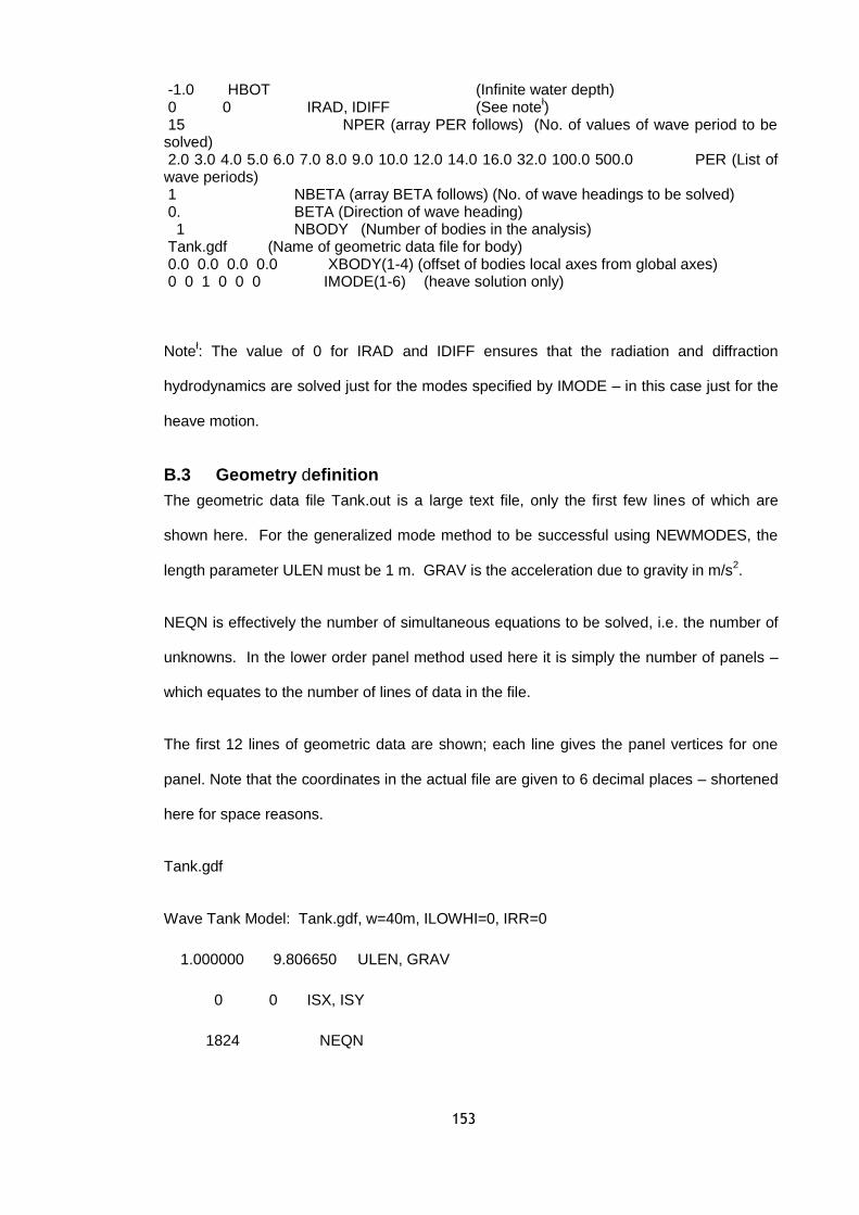
153

-1.0 HBOT (Infinite water depth) 0 0 IRAD, IDIFF (See note

ł)

15 NPER (array PER follows) (No. of values of wave period to be solved) 2.0 3.0 4.0 5.0 6.0 7.0 8.0 9.0 10.0 12.0 14.0 16.0 32.0 100.0 500.0 PER (List of wave periods) 1 NBETA (array BETA follows) (No. of wave headings to be solved) 0. BETA (Direction of wave heading) 1 NBODY (Number of bodies in the analysis) Tank.gdf (Name of geometric data file for body) 0.0 0.0 0.0 0.0 XBODY(1-4) (offset of bodies local axes from global axes) 0 0 1 0 0 0 IMODE(1-6) (heave solution only)

Noteł: The value of 0 for IRAD and IDIFF ensures that the radiation and diffraction

hydrodynamics are solved just for the modes specified by IMODE – in this case just for the

heave motion.

B.3 Geometry definition

The geometric data file Tank.out is a large text file, only the first few lines of which are

shown here. For the generalized mode method to be successful using NEWMODES, the

length parameter ULEN must be 1 m. GRAV is the acceleration due to gravity in m/s2.

NEQN is effectively the number of simultaneous equations to be solved, i.e. the number of

unknowns. In the lower order panel method used here it is simply the number of panels –

which equates to the number of lines of data in the file.

The first 12 lines of geometric data are shown; each line gives the panel vertices for one

panel. Note that the coordinates in the actual file are given to 6 decimal places – shortened

here for space reasons.

Tank.gdf

Wave Tank Model: Tank.gdf, w=40m, ILOWHI=0, IRR=0

1.000000 9.806650 ULEN, GRAV

0 0 ISX, ISY

1824 NEQN

154

2.74 1.00 -11.78 2.74 0.00 -11.78 2.35 0.00 -12.86 2.35 1.00 -12.86

3.13 1.00 -10.71 3.13 0.00 -10.71 2.74 0.00 -11.78 2.74 1.00 -11.78

3.52 1.00 -9.64 3.52 0.00 -9.64 3.13 0.00 -10.71 3.13 1.00 -10.71

3.91 1.00 -8.57 3.91 0.00 -8.57 3.52 0.00 -9.64 3.52 1.00 -9.64

4.30 1.00 -7.50 4.30 0.00 -7.50 3.91 0.00 -8.57 3.91 1.00 -8.57

4.69 1.00 -6.43 4.69 0.00 -6.43 4.30 0.00 -7.50 4.30 1.00 -7.50

5.08 1.00 -5.36 5.08 0.00 -5.36 4.69 0.00 -6.43 4.69 1.00 -6.43

5.47 1.00 -4.29 5.47 0.00 -4.29 5.08 0.00 -5.36 5.08 1.00 -5.36

5.86 1.00 -3.21 5.86 0.00 -3.21 5.47 0.00 -4.29 5.47 1.00 -4.29

6.25 1.00 -2.14 6.25 0.00 -2.14 5.86 0.00 -3.21 5.86 1.00 -3.21

6.64 1.00 -1.07 6.64 0.00 -1.07 6.25 0.00 -2.14 6.25 1.00 -2.14

7.03 1.00 0.00 7.03 0.00 0.00 6.64 0.00 -1.07 6.64 1.00 -1.07

X1 Y1 Z1 X2 Y2 Z2 X3 Y3 Z3 X4 Y4 Z4

B.4 Force Control file

The format of the Force Control File is in accordance with “Alternative form 2”, since

IALTFRC=2 in the control file, Tank.cfg. The chosen IOPTN options control the evaluation

and output of the following quantities:

Added-mass and damping coefficients output file: Tank.1 Exciting forces from Haskind relations output file: Tank.2 Exciting forces from diffraction potential output file: Tank.3 Motions of body (response amplitude operator) output file: Tank.4 The total mass of the device is 5423.11 tonne and the figures for rotary inertia are based on

arbitrarily chosen values of radius of inertia, k , as follows:

Rotation about x-axis (roll): kxx= 5 m thus inertia, Ixx= 1.35577e8 kg m2

Rotation about y-axis (pitch): kyy= 5 m thus inertia, Iyy= 1.35577e8 kg m2

Rotation about x-axis (roll): kzz= 4 m thus inertia, Izz= 8.67697e7 kg m2

155

It needs to be pointed out that these inertia values are not correct, but were chosen during

the de-bugging exercise when comparing the WAMIT and AQWA models. This does not

affect the validity of the analyses in this document which consider the heave motion alone.

However, realistic inertia values were used in the design calculations to assess the stability

and resonant periods in roll, pitch and yaw of the wave tank model. The damping and

stiffness values are those for mode 7, the Clam PTO. Thus in this example the PTO

damping is 4e5 Ns/m and its stiffness is 1.5e6 N/m .

Tank.frc

Wave Tank Model: Tank.frc, w=40m, ILOWHI=0, IRR=0 1 1 1 1 0 0 0 0 0 IOPTN(1-9) 1000.0 RHO (Density of water – fresh water, as in wave tank) 0.0 0.0 -12.0 XCG YCG ZCG (C of G is 12 m below waterline) 1 IMASS

5.42311e6 .0000000 .0000000 .0000000 .0000000 .0000000 .0000000 .0000000 5.42311e6 .0000000 .0000000 .0000000 .0000000 .0000000 .0000000 .0000000 5.42311e6 .0000000 .0000000 .0000000 .0000000 .0000000 .0000000 .0000000 1.35577e8 .0000000 .0000000 .0000000 .0000000 .0000000 .0000000 .0000000 1.35577e8 .0000000 .0000000 .0000000 .0000000 .0000000 .0000000 .0000000 8.67697e7 .0000000 .0000000 .0000000 .0000000 .0000000 .0000000 .0000000 .0000000 EXMASS (7x7) 1 IDAMP

.0000000 .0000000 .0000000 .0000000 .0000000 .0000000 .0000000 .0000000 .0000000 .0000000 .0000000 .0000000 .0000000 .0000000 .0000000 .0000000 .0000000 .0000000 .0000000 .0000000 .0000000 .0000000 .0000000 .0000000 .0000000 .0000000 .0000000 .0000000 .0000000 .0000000 .0000000 .0000000 .0000000 .0000000 .0000000 .0000000 .0000000 .0000000 .0000000 .0000000 .0000000 .0000000 .0000000 .0000000 0.00000 .0000000 .0000000 .0000000 4.0e5 EXDAMP (7x7) 1 ISTIF

.0000000 .0000000 .0000000 .0000000 .0000000 .0000000 .0000000 .0000000 .0000000 .0000000 .0000000 .0000000 .0000000 .0000000 .0000000 .0000000 .0000000 .0000000 .0000000 .0000000 .0000000 .0000000 .0000000 .0000000 .0000000 .0000000 .0000000 .0000000 .0000000 .0000000 .0000000 .0000000 .0000000 .0000000 .0000000 .0000000 .0000000 .0000000 .0000000 .0000000 .0000000 .0000000 .0000000 .0000000 .0000000 .0000000 .0000000 .0000000 1.5e6 EXSTIF (7x7) 0 NBETAH (No. of Haskind wave headings, see note below) 0 NFIELD (No. of points in fluid domain to analyse wave elevation etc.)

Note: The user guide says: “The Haskind wave headings may be introduced in the Force

Control File as an option, to enable evaluations to be made of the Haskind exciting forces

156

(Option 2) and body motions in waves (Option 4) at heading angles not included in the

Potential Control File”. However, the Tank.pot file does specify a wave heading of 0°.

B.5 NEWMODES data file

This file contains geometric data that is input by the specially written FORTRAN subroutine

Newmodes.f that calculates VELH ZDISP, see Section ‎3.4. The length data is in metres

and the angles are degrees.

Tank_GeomData.dat

GeomData.DAT for Wave Tank Model 12.0 13.0 20.0 40.0 2.0 2.5 (HWATER, HPTO, THETA1, THETA2, ALENGTH,

BLENGTH)

Figure B.1: Input parameters for Newmodes.f

B.6 Output from WAMIT model

WAMIT produces a number of output files in line with the control data in Tank.cfg and

Tank.pot, see Section ‎B.2. The main output file that is always written (and which contains

most of the data of interest) is Tank.out. Also the file, wamitlog.txt contains information on

the progress of the computation and useful data should the run not be completed.

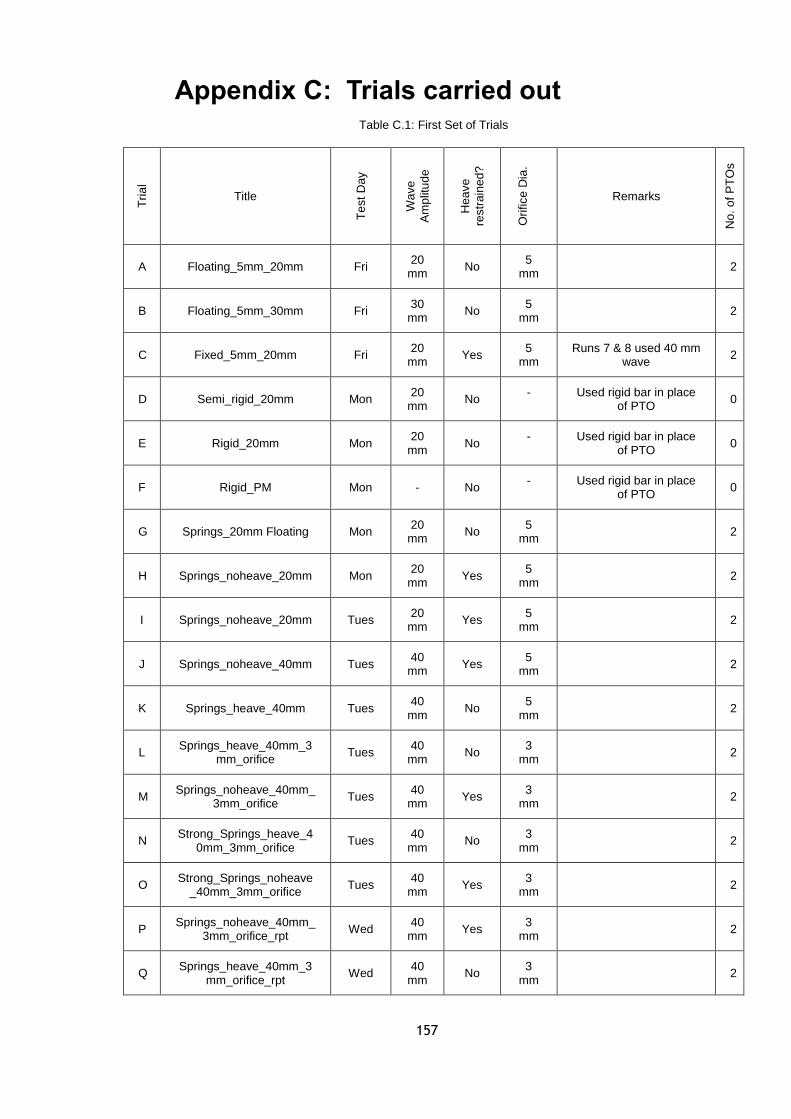
157

Appendix C: Trials carried out Table C.1: First Set of Trials

Tri

al

Title

Te

st

Day

Wa

ve

Am

plit

ud

e

He

ave

restr

ain

ed?

Ori

fice

Dia

.

Remarks

No

. o

f P

TO

s

A Floating_5mm_20mm Fri 20

mm No

5 mm

2

B Floating_5mm_30mm Fri 30

mm No

5 mm

2

C Fixed_5mm_20mm Fri 20

mm Yes

5 mm

Runs 7 & 8 used 40 mm wave

2

D Semi_rigid_20mm Mon 20

mm No

- Used rigid bar in place of PTO

0

E Rigid_20mm Mon 20

mm No

- Used rigid bar in place of PTO

0

F Rigid_PM Mon - No - Used rigid bar in place

of PTO 0

G Springs_20mm Floating Mon 20

mm No

5 mm

2

H Springs_noheave_20mm Mon 20

mm Yes

5 mm

2

I Springs_noheave_20mm Tues 20

mm Yes

5 mm

2

J Springs_noheave_40mm Tues 40

mm Yes

5 mm

2

K Springs_heave_40mm Tues 40

mm No

5 mm

2

L Springs_heave_40mm_3

mm_orifice Tues

40 mm

No 3

mm 2

M Springs_noheave_40mm_

3mm_orifice Tues

40 mm

Yes 3

mm 2

N Strong_Springs_heave_4

0mm_3mm_orifice Tues

40 mm

No 3

mm 2

O Strong_Springs_noheave

_40mm_3mm_orifice Tues

40 mm

Yes 3

mm 2

P Springs_noheave_40mm_

3mm_orifice_rpt Wed

40 mm

Yes 3

mm 2

Q Springs_heave_40mm_3

mm_orifice_rpt Wed

40 mm

No 3

mm 2

158

R FinalConfig_noheave_40

mm_wave_2_5mm_orifice Wed

40 mm

Yes 2.5 mm

1

S FinalConfigP_M_noheave_40mm_wave_2_5mm_o

Wed 40

mm Yes

2.5 mm

1

T Heave Response in Still

Water Wed N/A N/A

- 3 configs – Clam open, closed and central

-

Table C.2: Second Set of Trials

Tri

al

Title

Te

st

Day

Wa

ve

Am

plit

ud

e,

mm

Wa

ve

Dir

ectio

n

Ori

fice

Dia

., m

m

Sp

rin

g T

ype

Remarks

1,

1R

Const_5mm_20mm Wed 20 0° 5 C F

Nomenclature:

R – repeat

C F – Constant Force Spring

Coil – Coil spring: force varies linearly with

displacement

PM – Pierson-Moskowitz wave

spectrum

All wave inputs are regular except where

PM is indicated

2,

2R

Const_5mm_20mm_15deg

Wed 20 15° 5 C F

3,3

R


Wed 20 30° 5 C F

4,4

R

Const_5mm_Run PM2

Wed N/A 0° 5 C F

5,

5R

CoilSpring_5mm_20mm

Wed 20 0° 5

Coil

6 CoilSpring_5mm_

RunPM2 Wed N/A 0° 5

Coil

7 CoilSpring_3mm_

20mm Thurs 20 0° 3

Coil

8 CoilSpring_3mm_

20mm Thurs 20 0° 3

Coil

9 CoilSpring_3mm_20mm_Run2

Thurs 20 0° 3

Coil

159

10 CoilSpring_3mm_20

mm_15deg Thurs 20 15° 3

Co

il

11 CoilSpring_3mm_20

mm_30deg Thurs 20 30° 3

Co

il

12 CoilSpring_3mm_

20mm _RunPM2 Thurs N/A 0° 3

Co

il

13 CoilSpring_3mm_

20mm_RunPM2_ Spread

Thurs N/A 0° 3

Co

il

14 CoilSpring_3mm_

30mm Thurs 30 0° 3

Co

il

15

, 1

5R

Const_3mm_20mm Thurs 20 0° 3 C F

16

A,B

,C


Fri 20 15° 3 C F

17 Const_2_5mm_

20mm Fri 20 0° 2.5 C

F

18 Const_2_5mm_

20mm_15deg Fri 20 15° 2.5 C

F

19 Const_2_5mm_

20mm_30deg Fri 20 30° 2.5 C

F

20 Const_2_5mm_

RunPM2 Fri N/A 0° 2.5 C

F

21 Const_2_5mm_Run

PM2_Spread Fri N/A 0° 2.5 C

F

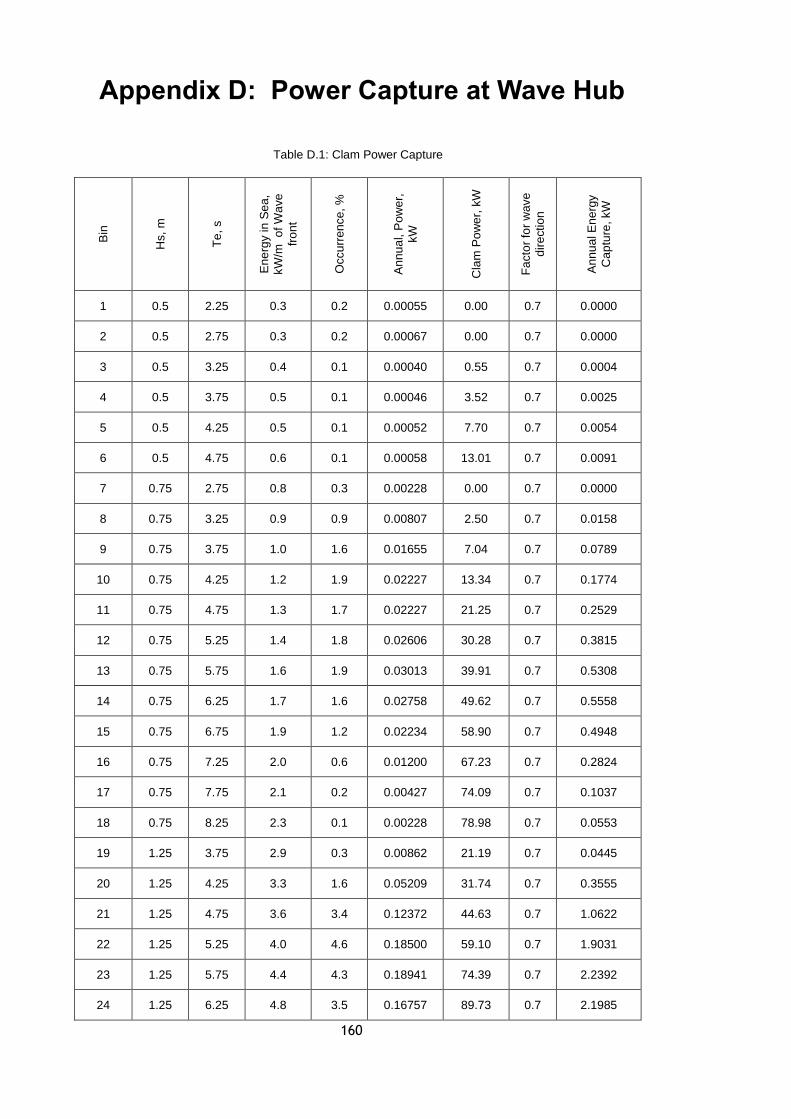
160

Appendix D: Power Capture at Wave Hub

Table D.1: Clam Power Capture

Bin

Hs,

m

Te

, s

En

erg

y in

Se

a,

kW

/m

of W

ave

fro

nt

Occu

rren

ce

, %

An

nu

al, P

ow

er,

kW

Cla

m P

ow

er,

kW

Fa

cto

r fo

r w

ave

dir

ectio

n

An

nu

al E

ne

rgy

Ca

ptu

re, kW

1 0.5 2.25 0.3 0.2 0.00055 0.00 0.7 0.0000

2 0.5 2.75 0.3 0.2 0.00067 0.00 0.7 0.0000

3 0.5 3.25 0.4 0.1 0.00040 0.55 0.7 0.0004

4 0.5 3.75 0.5 0.1 0.00046 3.52 0.7 0.0025

5 0.5 4.25 0.5 0.1 0.00052 7.70 0.7 0.0054

6 0.5 4.75 0.6 0.1 0.00058 13.01 0.7 0.0091

7 0.75 2.75 0.8 0.3 0.00228 0.00 0.7 0.0000

8 0.75 3.25 0.9 0.9 0.00807 2.50 0.7 0.0158

9 0.75 3.75 1.0 1.6 0.01655 7.04 0.7 0.0789

10 0.75 4.25 1.2 1.9 0.02227 13.34 0.7 0.1774

11 0.75 4.75 1.3 1.7 0.02227 21.25 0.7 0.2529

12 0.75 5.25 1.4 1.8 0.02606 30.28 0.7 0.3815

13 0.75 5.75 1.6 1.9 0.03013 39.91 0.7 0.5308

14 0.75 6.25 1.7 1.6 0.02758 49.62 0.7 0.5558

15 0.75 6.75 1.9 1.2 0.02234 58.90 0.7 0.4948

16 0.75 7.25 2.0 0.6 0.01200 67.23 0.7 0.2824

17 0.75 7.75 2.1 0.2 0.00427 74.09 0.7 0.1037

18 0.75 8.25 2.3 0.1 0.00228 78.98 0.7 0.0553

19 1.25 3.75 2.9 0.3 0.00862 21.19 0.7 0.0445

20 1.25 4.25 3.3 1.6 0.05209 31.74 0.7 0.3555

21 1.25 4.75 3.6 3.4 0.12372 44.63 0.7 1.0622

22 1.25 5.25 4.0 4.6 0.18500 59.10 0.7 1.9031

23 1.25 5.75 4.4 4.3 0.18941 74.39 0.7 2.2392

24 1.25 6.25 4.8 3.5 0.16757 89.73 0.7 2.1985

161

25 1.25 6.75 5.2 2.9 0.14995 104.3 0.7 2.1185

26 1.25 7.25 5.6 2.4 0.13329 117.5 0.7 1.9741

27 1.25 7.75 5.9 1.6 0.09499 128.4 0.7 1.4381

28 1.25 8.25 6.3 1 0.06320 136.3 0.7 0.9542

29 1.25 8.75 6.7 0.6 0.04022 141.1 0.7 0.5928

30 1.25 9.25 7.1 0.3 0.02126 143.4 0.7 0.3012

31 1.25 9.75 7.5 0.1 0.00747 143.7 0.7 0.1006

32 1.75 4.75 7.1 0.4 0.02853 81.84 0.7 0.2291

33 1.75 5.25 7.9 2 0.15765 100.8 0.7 1.4123

34 1.75 5.75 8.6 3.3 0.28490 120.6 0.7 2.7879

35 1.75 6.25 9.4 3.7 0.34721 140.3 0.7 3.6360

36 1.75 6.75 10.1 3.2 0.32431 159.1 0.7 3.5640

37 1.75 7.25 10.9 2.7 0.29391 175.9 0.7 3.3258

38 1.75 7.75 11.6 2.1 0.24436 190.1 0.7 2.7945

39 1.75 8.25 12.4 1.6 0.19819 200.6 0.7 2.2475

40 1.75 8.75 13.1 1 0.13138 207.5 0.7 1.4528

41 1.75 9.25 13.9 0.6 0.08333 211.3 0.7 0.8875

42 1.75 9.75 14.6 0.3 0.04392 212.6 0.7 0.4465

43 1.75 10.3 15.4 0.1 0.01539 212.1 0.7 0.1485

44 1.75 10.8 16.1 0.1 0.01614 210.3 0.7 0.1473

45 2.25 5.25 13.0 0.1 0.01303 160.6 0.7 0.1124

46 2.25 5.75 14.3 0.8 0.11417 183.3 0.7 1.0269

47 2.25 6.25 15.5 2.4 0.37230 205.7 0.7 3.4559

48 2.25 6.75 16.8 2.6 0.43559 226.8 0.7 4.1278

49 2.25 7.25 18.0 2.2 0.39588 245.8 0.7 3.7865

50 2.25 7.75 19.2 1.9 0.36547 262.1 0.7 3.4866

51 2.25 8.25 20.5 1.5 0.30715 274.8 0.7 2.8860

52 2.25 8.75 21.7 1.2 0.26061 283.8 0.7 2.3845

53 2.25 9.25 23.0 0.8 0.18367 289.6 0.7 1.6221

54 2.25 9.75 24.2 0.3 0.07260 292.7 1.0 0.8782

55 2.25 10.3 25.4 0.1 0.02544 293.6 1.0 0.2936

162

56 2.25 10.8 26.7 0.1 0.02668 292.7 1.0 0.2928

57 2.75 6.25 23.17 0.3 0.06952 287.6 0.7 0.6041

58 2.75 6.75 25.0 1.4 0.35037 301.0 1.0 4.2143

59 2.75 7.25 26.9 1.9 0.51073 330.2 1.0 6.2734

60 2.75 7.75 28.7 1.7 0.48849 347.5 1.0 5.9084

61 2.75 8.25 30.6 1.3 0.39765 361.5 1.0 4.7005

62 2.75 8.75 32.4 0.9 0.29198 372.1 1.0 3.3491

63 2.75 9.25 34.3 0.7 0.24007 379.4 1.0 2.6563

64 2.75 9.75 36.1 0.5 0.18075 383.9 1.0 1.9197

65 2.75 10.3 38.0 0.3 0.11401 385.8 1.0 1.1575

66 2.75 10.8 39.9 0.1 0.03986 385.4 1.0 0.3854

67 3.25 6.75 35.0 0.2 0.06991 410.2 1.0 0.8205

68 3.25 7.25 37.5 0.9 0.33790 431.5 1.0 3.8835

69 3.25 7.75 40.1 1.3 0.52173 449.3 1.0 5.8421

70 3.25 8.25 42.7 1.1 0.46995 463.4 1.0 5.0976

71 3.25 8.75 45.3 0.8 0.36249 473.5 1.0 3.7879

72 3.25 9.25 47.9 0.6 0.28741 479.8 1.0 2.8791

73 3.25 9.75 50.5 0.4 0.20196 482.8 1.0 1.9312

74 3.25 10.3 53.1 0.2 0.10616 482.6 1.0 0.9652

75 3.25 10.8 55.7 0.1 0.05567 479.5 1.0 0.4796

76 3.25 11.3 58.3 0.1 0.05826 473.9 1.0 0.4740

77 3.75 7.25 50.0 0.1 0.04998 552.4 1.0 0.5525

78 3.75 7.75 53.4 0.7 0.37402 570.7 1.0 3.9952

79 3.75 8.25 56.9 1 0.56879 582.9 1.0 5.8297

80 3.75 8.75 60.3 0.7 0.42228 589.1 1.0 4.1239

81 3.75 9.25 63.8 0.5 0.31887 589.8 1.0 2.9493

82 3.75 9.75 67.2 0.3 0.20166 585.8 1.0 1.7575

83 3.75 10.3 70.7 0.2 0.14134 577.7 1.0 1.1554

84 3.75 10.8 74.1 0.1 0.07412 566.1 1.0 0.5662

85 3.75 11.3 77.6 0.1 0.07756 551.9 1.0 0.5519

86 4.25 7.75 68.6 0.1 0.06863 714.2 1.0 0.7143

163

87 4.25 8.25 73.1 0.5 0.36529 722.4 1.0 3.6123

88 4.25 8.75 77.5 0.7 0.54240 719.9 1.0 5.0395

89 4.25 9.25 81.9 0.5 0.40957 708.3 1.0 3.5418

90 4.25 9.75 86.3 0.3 0.25902 689.4 1.0 2.0684

91 4.25 10.3 90.8 0.1 0.09077 664.9 1.0 0.6650

92 4.25 10.8 95.2 0.1 0.09520 636.5 1.0 0.6366

93 4.75 8.25 91.3 0.1 0.09126 875.6 1.0 0.8756

94 4.75 8.75 96.8 0.3 0.29037 860.2 1.0 2.5806

95 4.75 9.25 102.3 0.4 0.40928 830.6 1.0 3.3226

96 4.75 9.75 107.9 0.3 0.32356 790.2 1.0 2.3708

97 4.75 10.3 113.4 0.1 0.11338 742.3 1.0 0.7424

98 4.75 10.8 118.9 0.1 0.11891 690.2 1.0 0.6903

99 5.25 9.25 125.0 0.2 0.24999 948.4 1.0 1.8969

100 5.25 9.75 131.8 0.3 0.39526 884.9 1.0 2.6547

101 5.25 10.3 138.5 0.1 0.13851 812.0 1.0 0.8121

102 5.75 9.75 158.0 0.1 0.15804 970.0 1.0 0.9700

103 5.75 10.3 166.1 0.1 0.16615 876.3 1.0 0.8763

104 6.25 10.3 196.3 0.1 0.19630 937.4 1.0 0.9375

Total %: 99.3 18.0

179.5

Annual Power, kW/m

Mean Annual Power

Capture, kW

i This copy of the thesis has been supplied on condition that ...

Documents

Transcript of i This copy of the thesis has been supplied on condition that ...