CHAPTER 6

Hydrosphere

1.0. NRIAGU, C.E. REES, V.L. MEKHTIYEVA,A. Yu. LEIN, P. FRITZ, R.l.DRIMMIE, R.G. PANKINA, R.W. ROBINSON,AND H.R. KROUSE

6.1 INTRODUCTION*

Although isotope hydrology is a well-established field, the sulphur isotopesystematics of natural waters have not been extensively studied. The isotopiccomposition of sulphur in sea water is remarkably constant, and that ofsulphur in fresh waters so variable that it is difficult to gain fundamentalinsights of key processes and pathways. With the exception of the pioneeringwork of Deevey and his collaborators in the early 1960s (see Section 6.4),little was published on the isotope geochemistry of sulphur compounds inunpolluted freshwater ecosystems until the early 1970s.

With the recent development of 'environmental isotope' techniques, anumber of detailed investigations were undertaken to (a) identify sourcesof sulphur; (b) determine the pollution component; and (c) trace the fateof sulphur in aquatic ecosystems. Simultaneously, significant advances weremade in the use of sulphur and oxygen isotopes as complimentary tools inother areas of applied geochemistry. Of particular interest is the use ofisotopic techniques to (a) 'date' ground water; (b) identify the recharge areaand origin of sulphur; (c) infer groundwater circulation patterns, and (d)evaluate the migration rate, reactions, and extent of equilibration of thesulphur compounds (see Section 6.7).

More recently, interest in sulphur isotope measurements has beenheightened by the association of sulphur pollution with acid rain. Acid rainis threatening fisheries' resources and water quality of many lakes and riversin Europe and North America. Variations in the isotope abundances ofsulphur and oxygen in sulphate and sulphur oxides are ideally suited foracid rain studies. Isotopic compositions can be used for fingerprinting thesources of sulphur pollution as well as monitoring the long-range andtransboundary movement of the pollutant sulphur. This chapter includesillustrative case studies pertaining to stable sulphur/oxygen isotopes inrelation to lake and river acidification.

* J.O. Nriagu.

Stable Isotopes in the Assessment of Natural and Anthropogenic Sulphur in the EnvironmentEdited by H.R. Krouse and V.A. Grinenko<9 1991 SCOPE, Published by John Wiley & Sons Ltd

178 Stable Isotopes

Foremost, this chapter should serve to emphasize the fact that sulphur/oxygen isotopy provides the basis for a powerful but undeveloped tool inthe aquatic sciences. Only recently have sulphur isotopes been applied tofoodweb studies. Furthermore, the available data are sparse and focusmainly on local areas in Europe and North America. Little has been doneon sulphur isotope systematics in the ecosystems of developing countries.With the current data base, it would be premature to attempt even arudimentary model of sulphur isotope balance on a regional or global scale.An isotopic balance model should constrain current estimates of sources(natural versus anthropogenic) and elucidate sulphur transfer processes andthe rates of sulphur turnover in natural waters. In other words, it shouldprovide much needed checks for various models of the global sulphur cycle.

6.2 OCEANS

6.2.1 Dissolved sulphate*

Sulphur is present in the ocean in the form of dissolved sulphates,predominantly NaS04 -, MgS04°, CaS04 -, KS04 -, and SOi- (Garrelsand Thompson, 1962; Kester and Pytkowicz, 1969), with an averageconcentration of 0.904 g S kg-l (Horn, 1969). Taking the mass of water inthe world ocean to be 1.43 x 1012Tg gives the total mass of sulphate sulphuras 1.277 x 109Tg S (Horn, 1969). The flux of sulphur to and from theocean is ~300 Tg S yr-I (see below) so that the residence time of sulphurin the ocean is ~ 1.277 X 109 Tg S -7-300 Tg S yC 1 or ~4 X 106 yr.

In contrast to the long residence time of sulphate in the ocean, therelatively short oceanic mixingtime of ~ 1000years ensures that the sulphurisotopic composition of ocean sulphate is essentially uniform except inregions where local influences such as the mouths of rivers are important.

Measurements of the 034Svalues of suites of ocean water samples havebeen made by Ault and Kulp (1959), Thode et at. (1961), Sasaki (1972),and Rees et at. (1978). The results of these studies are summarized in Table6.1. The mean values obtained in the first three studies agree very wellwhereas the decrease in the spreads of 034Svalues obtained in successivestudies is indicative of the improvement with time of analytical precision.

The mean value of +20.99%0 obtained by Rees et at. (1978) is markedlydifferent from the mean values of around +20.0%0 obtained in the earlierstudies. This difference is due to the fact that this latter study was madeusing sulphur hexafluoride (SF6) as the gas for isotope analysis whereas theprevious studies employed sulphur dioxide (S02). Rees (1978, Section 2.1)

* C.E Rees.

Hydrosphere 179

Table 6.1 Summary of 834Sdeterminations for present-day ocean water sulphate

points out that results obtained using SF6 are more precise and, moreimportantly, more accurate than those obtained using S02'

It is of interest to speculate on whether the sulphur isotope compositionof present-day ocean sulphate is constant or if its 034S value is increasingor decreasing with time.

The 034S value of ocean water sulphate is controlled by the magnitudesof the various fluxes to and from the oceanic sulphate reservoir and by theisotopic compositions of these fluxes. Examination of the 034S values ofevaporitic sulphates which were derived from the dissolved sulphate inancient oceans has shown that the isotopic composition of oceanic sulphatehas not been constant over geological time (Thode and Monster, 1964, 1965;Nielsen, 1965; Holser and Kaplan, 1966; Schidlowski et al., 1977; Claypoolet al., 1980). The implication of these variations in terms of variations ofthe relative rates of evaporite and sedimentary sulphide formation, as wellas of the global atmospheric oxygen budget, has been discussed by theauthors cited above and by Rees (1970) and Holland (1973). The topic iscovered in detail by Pilot (Section 4.2).

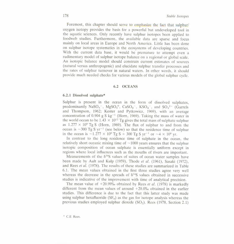
With regard to the present-day ocean, it is important to note that itssulphate content is possibly not in balance. Table 6.2 contains some fluxdata taken from Table 7.1 of Ivanov (1983). Some of the individual fluxeslisted by Ivanov have been combined for the purpose of the calculationsdeveloped later in this section. The total flux of sulphur to the ocean(P 10 + P20) is estimated to be ~480 Tg S yr-l while the total flux of sulphurfrom the ocean (PIs + PI9 + P21 + P22) is estimated to be ~Tg S yr-I.Thus the estimated input exceeds the estimated ouput by ~ 180Tg S yr-Ior ~60%.

Number Range of Spread ofof samples 834Svalues 834S Mean 834S (J" (JbIn I

Study N (%0) (%0) (%0) (%0) (%0)

Ault and Kulp +18.9 to

(1959) 25 +20.7 1.8 +20.0 0.1 0.54Thode et ai. +19.3 to

(1961) 16 20.8 1.5 +20.1 0.10 0.38+19.62 to

Sasaki (1972) 20 20.32 0.70 +20.03 0.05 0.21+20.74 to

Rees et ai. (1978) 25 +21.12 0.38 + 20.99 0.02 0.08

a Standard deviation of the mean.b Standard deviation of an individual determination 0"; = O"mYN.

Table 6.2 Calculations of the rate of change of the present-day O,4S value of ocean water sulphate >--'000

Flux values (Tg S yr -I)

Fluxes This O,4S value

(Ivanov, 1983) work (%0) 1 2 3 4 5 6 7 8 9 10 11

------

Continental atmosphere to Pg Og = +5 110 160oceanic atmosphere (Px)and volcanic emissions (P17)

River (PIO) , underground PIO 010 = +5 220 270

runoff (PI I)' shoreabrasion (P13)

Biogenic emission to Pig 0/\ - ex 20 70

oceanic atmosphere (PIx)

Ocean spray sulphate to PI9 0/\ 140 190 19()oceanic atmosphere (PI9)

Atmospheric sulphur P211 OAT 260 310 3Wcompounds to ocean (P211)

Removal of reduced P21 0/\ - f3 110 160sulphur in sediments (P21)

Removal of sulphate in Pn 0/\ 30 80sediments (Pn)

- ----------

ex(%0) 15 20 15 15f3 (%0) 50 40 5()

-_._----

034Sof atmospheric sulphate (%0) +13.4 +12.1 + 13.4 + 12.2 + 14.6 + 13.4 + 13.4 + 13.4 + 13.0 + 13.4 + 14.6

034Socean sulphate (%0per million years) +0.2 0 -0.4 +0.6 +0.5 -0.1 +2.2 +0.2 +0.2 -0.6 +0.2

Hydrosphere 181

It is not clear whether this estimated difference between input and outputis real or if it is an artefact of the uncertainties in the individual flux

estimates. For example, previous estimates of the biogenic emission fromthe ocean have varied widely-170 Tg S yr-I (Eriksson, 1960),30 Tg S yr-I(Robinson and Robbins, 1970), 48 Tg S yr-I (Friend, 1973), 27 Tg S yr-l(Granat et al., 1976). Recently Nguyen et al. (1978) have estimated a marineflux of dimethyl sulphide (DMS) of at least 89 Tg S yr-l, possibly in additionto other biological contributions.

Because there are uncertainties in the various flux estimates, calculationsare performed below to determine the rate of change with time of thepresent-day 034S value of oceanic sulphate for both the flux estimatespresented by Ivanov (1983) and for other possible values.

Let A represent the present-day value of the sulphate sulphur content ofthe ocean and let Ii> Fj (i = 1,2,...; j = 1,2, . . .) represent the variouspresent-day fluxes of sulphur into (1) and from (F) the ocean. The rate ofchange of A with time is

dA = 2.Ii - 2. Fkdt i J

For 32S and 34S write

32

d32A = 2. 32]i - 2. Fjdt i j

and

d34A = 2. 34]i - 2. 34Fjdt i j

This last equation can be expressed in terms of del values by writing

34A = 32A Ro(1 + OA)34] . = 321 R (1 + 0, )I I 0 i

and

34 F. = 32FR ( 1 + OF)J J 0 J

where Ro represents the 34Sf32Svalue of the standard reference material(Canyon Diablo troilite) and where °A, OJ,OFrepresent the fractional delvalues of A, J, and F relative to the standard reference material. Makingthese substitutions in the equation for d34A/dt gives

182 Stable Isotopes

dp2A Ro(l + OA)]= 2: 321iRo(1 + 01) - 2: 320 R,(1 + OFj)i ]

Cancelling Ro throughout and making the assumption that the behaviour ofthe element, A, and that of the abundant isotope, 32A, are essentiallyidentical gives

d[A(1 + OA)]= 2: li(1 + 01) - 2:0(1 + OF)dt i 1

so that, expanding the differential,

dA dOA '" '"(1 + OA)dt + A dt = L..li(1 + 01) - L..0(1 + OF)

[ ]

Using

dA = 2: Ii - 2: Fjdt i ]

and rearranging the previous equation gives

dOA '" '"A dt = L.. li(o/i - OA)- L.. 0 (OFj- OA)

[ ]

In Table 6.2, 034S assignments for the various sulphur fluxes are given.The assignment of +5%0 for PI',and PlOmay not be exact but will serve forcalculation purposes. The 034Svalue of the flux of atmospheric sulphate tothe ocean, P2o, is assumed to be equal to the 034S value of atmosphericsulphate and is designated OATin the table. It will be assumed that OATisdetermined by the various fluxes to the oceanic atmosphere:

" - osPs + OAPI9+(OA - ex)PIsUAT-

PS+PI9+P1S

This is equivalent to assuming that none of the fluxes from the reservoir ofoceanic atmospheric sulphate involves isotope fractionation relative to thatreservOir.

The equation for doA/dt can now be written as

dOAA dt = PIO(OIO - OA) + P20(OAT - OA)

Hydrosphere 183

- PIS(OA - IX - OA)- PI9(OA - OA)-P2I(OA - 13 - 8A) - P22(8A - 8A)

- PIO(81O - 8A) + P2o(8AT - 8A) + IX Pu-: + 13 P21

In this expression, IXrepresents the difference in 834Svalues of ocean watersulphate and the biogenic sulphur flux to the atmosphere, while 13representsthe difference in the 834Svalues of ocean water sulphate and sulphide beingdeposited in the ocean sediments.

Column 1 of Table 6.2 shows the flux values quoted by Ivanov (1983)rounded off to the nearest 10 Tg S yc 1. These fluxes, their assigned delvalues, and values for IX(15%0)and 13(50%0)were inserted in the equationsdeveloped above. The calculated values of 834Sfor the atmosphere and therate of change of 834Sof ocean sulphate are + 13.4 and +0.2%0 per millionyears respectively. The extent to which these values (tabulated at the bottomof column 1) are realistic depends on the accuracies of the assigned fluxesand del values.

Columns 2 to 10 show the effects of altering the various parametersindividually including IXand 13.Each flux is increased in turn by 50 Tg Syr-I. Thus, for example, column 4 shows that if all the parameters arecorrect except for the estimate for PIs (the biogenic emission of sulphur tothe atmosphere should be 70 Tg S yr-I rather than 20 Tg S yc1), then therate of change of 834Sof ocean sulphate should be +0.6 rather than +0.2%0per million years.

Column 11 differs from column 1 in that PI9 and P20 have been alteredtogether. Altering P19 alone changes the estimated rate of change of 834Sfrom +0.2 to +0.5%0 per million years (column 5). Alteration of P19 andP20 together gives no net change (compare column 1 with column 11).

The values in Table 6.2 show that it is not possible to state unequivocallywhether the 834Svalue of ocean sulphate is currently increasing, decreasing,or constant. A clear answer requires estimates of the various importantfluxes to a much higher degree of certainty than is presently possible.

6.2.2 Sulphur of aquatic organisms*

The hydrosphere is a major habitat which actively influences the distributionof chemical elements, particularly sulphur. The total S in animal and planttissue varies from less than 1 up to 9% by dry weight. On a dry weightbasis, the S content of aquatic plants and animal tissues varies from 0.5 to5 and 0.1 to 3.3% respectively (Vinogradov, 1953; Kaplan et al., 1963;Mekhtiyeva and Pankina, 1968; Mekhtiyeva et al., 1976; Mekhtiyeva, 1971).(Unless stated otherwise, percent S will be given on a dry weight basis.)

* V.L. Mekhtiyeva.

184 Stable Isotopes

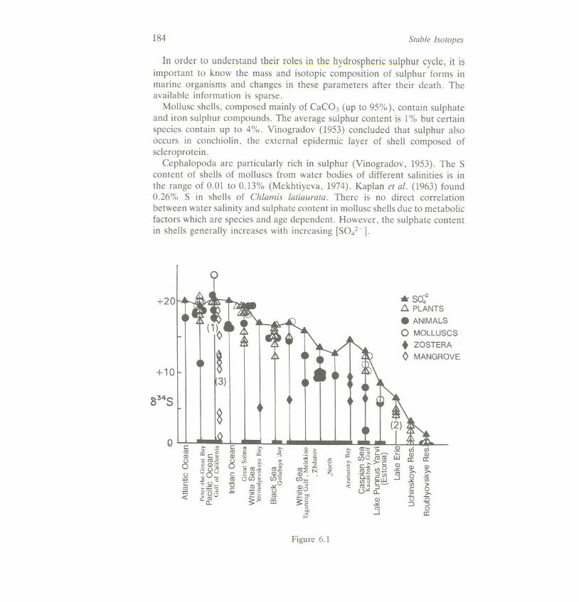
In order to understand their roles in the hydrospheric sulphur cycle, it isimportant to know the mass and isotopic composition of sulphur forms inmarine organisms and changes in these parameters after their death. Theavailable information is sparse.

Mollusc shells, composed mainly of CaC03 (up to 95%), contain sulphateand iron sulphur compounds. The average sulphur content is 1% but certainspecies contain up to 4%. Vinogradov (1953) concluded that sulphur alsooccurs in conchiolin, the external epidermic layer of shell composed ofscleroprotein.

Cephalopoda are particularly rich in sulphur (Vinogradov, 1953). The Scontent of shells of molluscs from water bodies of different salinities is in

the range of 0.01 to 0.13% (Mekhtiyeva, 1974). Kaplan et al. (1963) found0.26% S in shells of Chlamis latiaurata. There is no direct correlationbetween water salinity and sulphate content in mollusc shells due to metabolicfactors which are species and age dependent. However, the sulphate contentin shells generally increases with increasing [SOi-].

+10

. SO~2~ PLANTS. ANIMALS0 MOLLUSCS

. ZOSTERA

0 MANGROVE

3)

834S

~

Q I::coQ)U0.~c:.!!1;:(

»"'1::",» »oiJI::.§ m.§ oiJ ~'" co.E u r5i ~ ~~ ~~ 0 '" co~ co]00 U I:: ~ Q)go Q).=;i! '0 .!!1 0 Cf)!f, Cf)~<;'.~~ "0 Q) 0 ~

:;:t::; .£ .~E a;"uo .s:::,,-o..g: :5:>'- CD

0 >" 0

~ ~ ~"..c: 0CO:2: N zQ) . .

Cf)~

Q):;_0:E~:5:s

OJ,F"

» co::::.::;'" Q)" ~Cii~ Cf)~~.E~ ~~ 00.815 'a.~ ~ C{j;:: OON I::~« CO"::J

0'" a..Q)~coJ

Q) . cr.i.- 00 Q)Lu £ a:Q) Q) Q)~ ;>. ;>.co 0 ~

J ~ 0000 >I:: 0.- ;>..s::: -u .c:) ::J

0a:

Figure 6.1

Hydrosphere 185

The isotopic composition of sulphate in shells of molluscs is practicallyidentical to that of dissolved sulphate in their habitat (Kaplan et al., 1963;Mekhtiyeva, 1974; Figure 6.1). After an organism's death, the amount ofsulphur and 334Svalues in skeletons do not change. This fact may be usedfor palaeohydrochemical reconstructions of sediment accumulation in ancientbasins (Mekhtiyeva, 1974).

Trace sulphide and sulphate can be extracted from geological specimensusing Kiba reagent under vacuum conditions (Ueda and Sakai, 1983). Usingthis technique, a Puaua shell from New Zealand was found to have 334Svalues for sulphate (490 ppm S) and sulphide (30 ppm S) of +21.4 and+7.7%0 respectively (Krouse and Ueda, 1987). The error for the latter isrelatively large because of its low concentration.

The chitinic tubes of polychaeta are depleted in 34S by about 13%0compared to dissolved sulphate. This is apparently due to the presence ofpyrite inclusions (Kaplan et al., 1963).

Sulphur is generally supplied to plants in the form of sulphate which isreduced in the course of metabolism to thiol groups reacting with serine.As a result, cysteine is produced which is the precursor of the whole seriesof sulphur-containing amino acids. Natural thiols and disulphides are readilyoxidized to produce numerous derivatives of sulphur oxide compounds.

In addition to sulphate, plants may assimilate other sulphur compounds,including hydrogen sulphide (Thomas et al., 1943; Ellis, 1969; Faller, 1972;Brunold and Erisman, 1974, 1975; Fry et al., 1982; see also Chapter 7). Theisotopic composition of sulphur in aquatic plants is slightly lighter than thatof dissolved sulphate (Figure 6.1). The depletion in 34Sfor total sulphur in

40Pacific Ocean

Indian Ocean'

---0

'0'2-

;: 20I-Z:J«CJ)

. White Sea

. BlackSea

. AsovSea

Roublyovskoye Reservoir0 18 I I I

0 1 2 3SULPHUR CONTENT (%)

Figure 6.2

186 Stable Isotopes

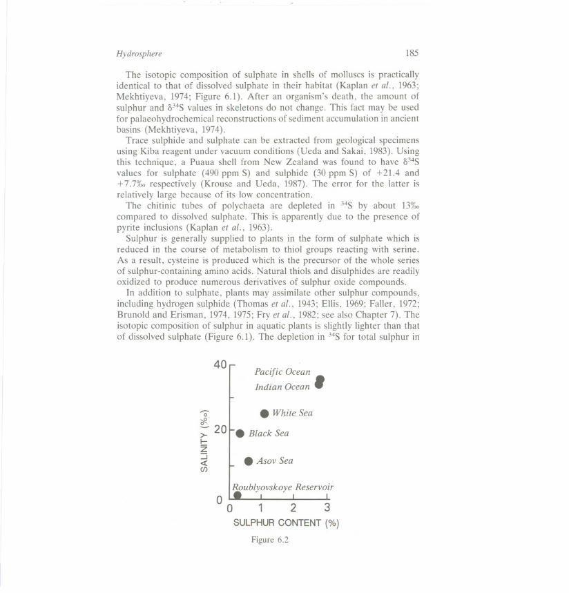
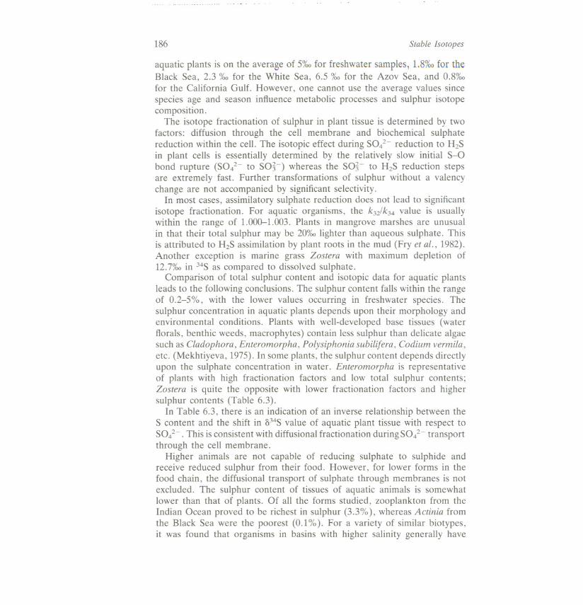
aquatic plants is on the average of 5%0for freshwater samples, 1.8%0for theBlack Sea, 2.3 %0for the White Sea, 6.5 %0for the Azov Sea, and 0.8%0for the California Gulf. However, one cannot use the average values sincespecies age and season influence metabolic processes and sulphur isotopecomposition.

The isotope fractionation of sulphur in plant tissue is determined by twofactors: diffusion through the cell membrane and biochemical sulphatereduction within the cell. The isotopic effect during SOi- reduction to H2Sin plant cells is essentially determined by the relatively slow initial S-Obond rupture (SOi- to SOj-) whereas the SOj- to H2S reduction stepsare extremely fast. Further transformations of sulphur without a valencychange are not accompanied by significant selectivity.

In most cases, assimilatory sulphate reduction does not lead to significantisotope fractionation. For aquatic organisms, the k32/k34 value is usuallywithin the range of 1.000-1.003. Plants in mangrove marshes are unusualin that their total sulphur may be 20%0lighter than aqueous sulphate. Thisis attributed to H2S assimilation by plant roots in the mud (Fry et al., 1982).Another exception is marine grass Zostera with maximum depletion of12.7%0in 34Sas compared to dissolved sulphate.

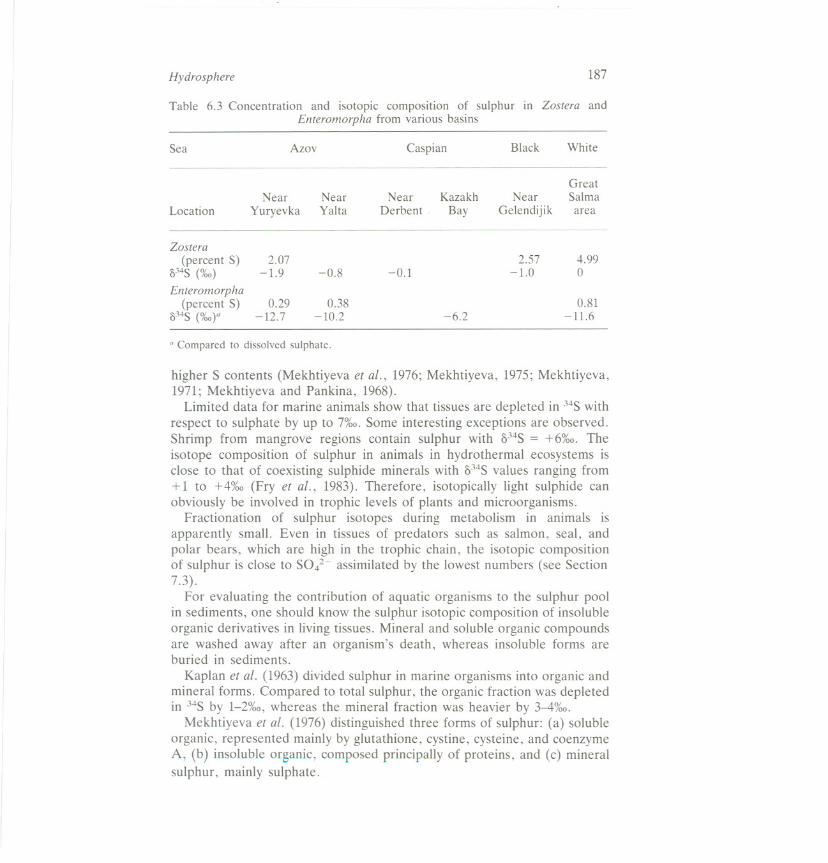
Comparison of total sulphur content and isotopic data for aquatic plantsleads to the following conclusions. The sulphur content falls within the rangeof 0.2-5%, with the lower values occurring in freshwater species. Thesulphur concentration in aquatic plants depends upon their morphology andenvironmental conditions. Plants with well-developed base tissues (waterflorals, benthic weeds, macrophytes) contain less sulphur than delicate algaesuch as Cladophora, Enteromorpha, Polysiphonia subilifera, Codium vermila,etc. (Mekhtiyeva, 1975). In some plants, the sulphur content depends directlyupon the sulphate concentration in water. Enteromorpha is representativeof plants with high fractionation factors and low total sulphur contents;Zostera is quite the opposite with lower fractionation factors and highersulphur contents (Table 6.3).

In Table 6.3, there is an indication of an inverse relationship between theS content and the shift in 834Svalue of aquatic plant tissue with respect toSOi-. This is consistent with diffusional fractionation duringSOi- transportthrough the cell membrane.

Higher animals are not capable of reducing sulphate to sulphide andreceive reduced sulphur from their food. However, for lower forms in thefood chain, the diffusional transport of sulphate through membranes is notexcluded. The sulphur content of tissues of aquatic animals is somewhatlower than that of plants. Of all the forms studied, zooplankton from theIndian Ocean proved to be richest in sulphur (3.3%), whereas Actinia fromthe Black Sea were the poorest (0.1%). For a variety of similar biotypes,it was found that organisms in basins with higher salinity generally have

Hydrosphere 187

Table 6.3 Concentration and isotopic composition of sulphur in Zostera andEnteromorpha from various basins

higher S contents (Mekhtiyeva et at., 1976; Mekhtiyeva, 1975; Mekhtiyeva,1971; Mekhtiyeva and Pankina, 1968).

Limited data for marine animals show that tissues are depleted in 34Swithrespect to sulphate by up to 7%0.Some interesting exceptions are observed.Shrimp from mangrove regions contain sulphur with 834S= +6%0. Theisotope composition of sulphur in animals in hydrothermal ecosystems isclose to that of coexisting sulphide minerals with 1)34Svalues ranging from+ 1 to +4%0 (Fry et at., 1983). Therefore, isotopically light sulphide canobviously be involved in trophic levels of plants and microorganisms.

Fractionation of sulphur isotopes during metabolism in animals isapparently small. Even in tissues of predators such as salmon, seal, andpolar bears, which are high in the trophic chain, the isotopic compositionof sulphur is close to SOi- assimilated by the lowest numbers (see Section7.3).

For evaluating the contribution of aquatic organisms to the sulphur poolin sediments, one should know the sulphur isotopic composition of insolubleorganic derivatives in living tissues. Mineral and soluble organic compoundsare washed away after an organism's death, whereas insoluble forms areburied in sediments.

Kaplan et at. (1963) divided sulphur in marine organisms into organic andmineral forms. Compared to total sulphur, the organic fraction was depletedin 34Sby 1-2%0, whereas the mineral fraction was heavier by 3-4%0.

Mekhtiyeva et at. (1976) distinguished three forms of sulphur: (a) solubleorganic, represented mainly by glutathione, cystine, cysteine, and coenzymeA, (b) insoluble organic, composed principally of proteins, and (c) mineralsulphur, mainly sulphate.

Sea Azov Caspian Black White

GreatNear Near Near Kazakh Near Salma

Location Yuryevka Yalta Derbent Bay Gelendijik area

Zostera(percent S) 2.07 2.57 4.99

034S (%0) -1.9 -0.8 -0.1 -1.0 0

Enteromorpha(percent S) 0.29 0.38 0.81

034S (%oY -12.7 -10.2 -6.2 -11.6

" Compared to dissolvedsulphate.

188 Stable Isotopes

In both plants and animals, insoluble organic sulphur compoundsdominate.The second important form is soluble organic sulphur compounds in animals,but sulphate in plants. In unpolluted environments, the 834S of the threesulphur forms are similar for a given specimen with maximum differencesof 4.8%0 for plants and 5.7%0 for animals. In all organisms, the solubleorganic sulphur (compared to total sulphur) is isotopically heavier, whereasthe insoluble fraction is lighter. Sulphate in plants is enriched in 34S,whereasin animals it has a variable composition compared to total sulphur. Thecomparative 34Senrichment in sulphate in plants is consistent with it beingthe residual of partial metabolism by the cell. Reduced sulphur is concentratedin proteins and thereafter it is transformed into soluble organic compoundswhich are dominantly oxidized forms. Sulphate in marine animals has a dualorigin. It is formed by oxidation of reduced forms and is also supplied fromsea water. This conclusion is corroborated by the direct dependence betweensulphur contents in animal tissues and [SOi-] in the environment.

Osmotic permeability of cell membranes differs in aquatic organisms. Theorganisms endowed with high permeability contain high concentrations ofsulphate (aspidium, starfish, and sea comb). Animals closely related inclassification, e.g. all fish species, and inhabiting similar environmentscontain nearly equal amounts of various forms of sulphur. Isotopic differencesbetween sulphur in aquatic organisms and the environment are essentiallydetermined by mechanisms of sulphate supply to cells.

The gross production of phytoplankton in oceans is assessed as2 x 104Tg Corgyr-l or 3.6 x 104Tg of organic matter (dry basis)(Romankevich, 1977). Volkov and Rozanov (1983) assume the averagesulphur content in phyto- and zooplankton to be 1%, which suggests that- 360 Tg S are contributed annually to the oceanic sulphur. Based onMekhtiyeva (1971), the average sulphur content in oceanic plankton isconsiderably higher (2.5-3.3%). This suggests that the annual production ofplanktonic sulphur in the oceans is about 103Tg. Neither estimate is wellfounded since there are no sulphur analyses from representative samples ofoceanic phytoplankton. Data are available on the content of sulphur inmixed samples of phyto- and zooplankton, and on the variable sulphurcontent in algae-macrophytes. The higher estimate appears to be moreprobable as the sulphur content in small plant forms with salt-permeableenvelopes is usually higher than in macrophytes.

According to Romankevich (1977), the annual production of phytobenthosin oceans is 300 Tg of dry matter. For an average sulphur content of 2%,this corresponds to 6 Tg of total sulphur or 4.2 Tg of insoluble organicsulphur per annum.

The above estimates suggest that the isotopic composition of total sulphurin aquatic organisms is quite close to that of water sulphate. For planktonicforms, the fractionation factor is 1.0034 (average of three measurements).

Hydrosphere 189

Insoluble organic sulphur, which accounts for about 70% of the total sulphurin aquatic organisms, is slightly lighter isotopically (up to 2%0)compared tototal sulphur. Decomposition of sulphur organic compounds from deadplankton occurring in the water column may lead to a heavier isotopiccomposition residual sulphur (by 1-2%0). Thus organic sulphur compoundssupplied to the oceans with particulate matter should have ~34Svalues closeto +16%0.

For benthic macrophytes, the fractionation factor is lower and in mostcases is close to 1.001. The bulk of the benthic biomass is formed by themost distributed oceanic algae Chlorophyta, Phaeophyta, and Rhodophyta,whereas contributions from Zostera and mangroves are insignificant. Anaverage ~34S value of + 18.5%0 is estimated for the biomass of benthicvegetation, whereas that of their organic sulphur derivatives may be assumedto be + 17%0. Dead plants are buried in the proximity of their habitat.Therefore, no significant changes in their mass and isotopic compositionoccur during the period from their death to burial.

6.3 MODERN OCEAN SEDIMENTS*

When preparing SCOPE 19, data reported up to 1980 were used to calculatethe isotopic balance of sulphur buried in oceanic sediments. New informationon the content of various sulphur forms in sediments, sulphur isotopiccomposition, and sulphate reduction (Lew, 1981; Lein et al., 1981; Chambers,1982; Skyring et al., 1983) warranted an updated review. Moreover, theprevious SCOPE report did not address fully the geochemical activity ofsulphate reducing bacteria in shallow oceanic waters. Interesting ecosystemssuch as sediments of marshes, tidal flats, and their North Europeananalogues, lidos, were not considered. Intensive sulphate reduction has beenstudied in these ecosystems in the United Kingdom (MacLeod, 1973; Nedwelland Abram, 1978, 1979; Banat et al., 1981; Nedwell and Banat, 1981),Atlantic USA (Calvert and Ford, 1973; Atkinson and Hall, 1976; Skyringet al., 1979; Shink, 1979; Howarth and Teal, 1979, 1980; Howarth et al.,1983; Stround and Paynter, 1980; King and Wiebe, 1980; Luther et al.,1982; Bouleque et al., 1982; Peterson et al., 1983; Howarth and Giblin,1983), Pacific USA (Kaplan et al., 1963), and Australia (Chambers, 1982;Skyring et al., 1983).

6.3.1 Intensity of sulphate reduction

Recent investigations showed that microbial sulphate reduction processesare abundant in bottom sediments of continental and marginal seas, various

* A. Yu. Lein.

190 Stable Isotopes

geomorphological zones of the ocean to depths of 3000-5000 m, and tolimited depths in deep-water trenches. The maximum depth at which sulphatereduction can occur in oceanic sediments has not been established but theprocess has been documented at a depth of 5-6 m from the silt surface anddown to 13 m in Baltic Sea sediments (Lein, 1983).

The intensity of microbial sulphide generation varies from less than1 J.LgS kg-1 d-1 in deep-water oceanic sediments to tens of mg S kg-l d-Iin sediments of the continental Baltic Sea.

However, the highest intensities of sulphide production are found inmarshes and tidal flats, including lowland plains along seashores, floodedduring high tides or storms. In marshes, soils rich in humus are formed onsilt and sand-silt drifts with high Corg content. Such sediments are typicalof lowland shores of Great Britain, the Federal Republic of Germany, theNetherlands, and sections of the Atlantic shore of the United States. Thetotal area of such high-tide and low-tide zones is estimated at 6 x 104 km2(Atlas of the Oceans, 1977).

Despite the large number of investigations, the isotopic composition ofsulphur has been studied only in sediments of Newport marsh, California,USA (Kaplan et al., 1963) and the Mambray Creek marsh of South Australia(Chambers, 1982).

In marsh sediments, the concentration of sulphate increases with depth.For example, in Newport marsh the sulphate sulphur content in the surfacehorizon is 0.073% as compared with 0.091% at 30 cm below the surface(Kaplan et al., 1963). Surface water and water squeezed out of green algaehad sulphate sulphur concentrations of 0.094 and 0.098% respectively.Therefore, the most active sulphate reduction occurs in the upper (10-20 cm)of marsh sediments. Lower in the column, in the sand underlying the surfacesilt, reduced sulphur is oxidized due to flushing with Oz-saturated H2O.Stratified sulphate reduction is characteristic of most marshes. This is alsoconfirmed by changes in Eh values from - 300 mV in upper horizons to+ 100 mV deep in the sediment (Table 6.4). The Corg and Spyritccontentsdecrease similarly from 1.7 and 0.92% (dry weight basis) in the upperhorizon to 0.4 and 0.3% at a depth of 30 cm (Table 6.4). The f>34Svaluesof pyrite change with depth from -20.0%0 (0-5 cm horizon) to -27.7%0(60-65 cm horizon). Just as in normal sea sediments, free H2S and acid-soluble sulphides are enriched in 34Sby 4-5%0 compared to pyrite sulphur(Table 6.4).

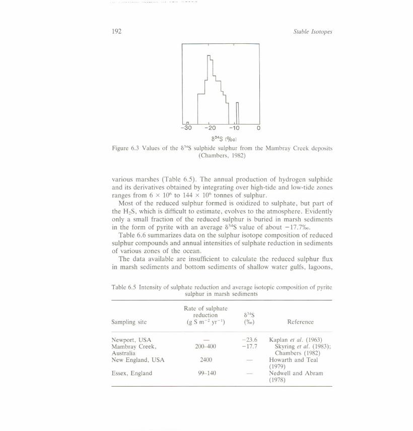
A comprehensive study of the sulphur cycle was carried out fromNovember 1977 to November 1978 in a lO-cm stratum of Mambray Creekmarsh sediments (Chambers, 1982). The f>34Svalues of pyrite varied from-9 to -27%0 (average -17.7%0, 80 determinations at three stations) (Figure6.3).

Rates of sulphate reduction, measured with 35S-labelled sulphate, rangedfrom 1.7 to 41 mg S kg-1 d-I or 100-2400 g S m-2 yr-l in sediments of

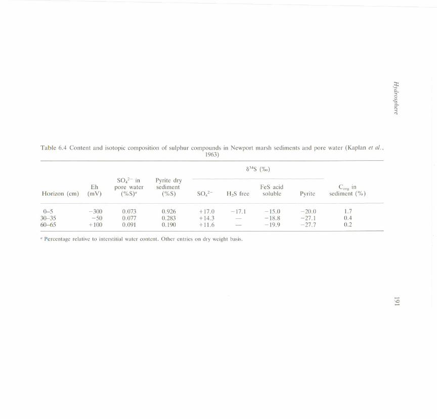
Table 6.4 Content and isotopic composition of sulphur compounds in Newport marsh sediments and pore water (Kaplan et al.,1963)

" Percentage relative to interstitial water content. Other entries on dry weight basis.

~""-

C3

{J:::-'"....'"

......\0......

534S (%0)

SO/- in Pyrite dryEh pore water sediment FeS acid Corg in

Horizon (cm) (mY) (%S)" (%S) SO/- H2S free soluble Pyrite sediment (%)

0-5 -300 0.073 0.926 + 17.0 -17.1 -15.0 -20.0 1.730-35 -50 0.077 0.283 +14.3 - -18.8 -27.1 0.460-65 +100 0.091 0.190 +11.6 - -19.9 -27.7 0.2

192 Stable Isotopes

-30 -20 -10 0

8348 (%0)

Figure 6.3 Values of the 334S sulphide sulphur from the Mambray Creek deposits(Chambers, 1982)

various marshes (Table 6.5). The annual production of hydrogen sulphideand its derivatives obtained by integrating over high-tide and low-tide zonesranges from 6 x 106 to 144 X 106 tonnes of sulphur.

Most of the reduced sulphur formed is oxidized to sulphate, but part ofthe HzS, which is difficult to estimate, evolves to the atmosphere. Evidentlyonly a small fraction of the reduced sulphur is buried in marsh sedimentsin the form of pyrite with an average 034Svalue of about -17.7%0.

Table 6.6 summarizes data on the sulphur isotope composition of reducedsulphur compounds and annual intensities of sulphate reduction in sedimentsof various zones of the ocean.

The data available are insufficient to calculate the reduced sulphur fluxin marsh sediments and bottom sediments of shallow water gulfs, lagoons,

Table 6.5 Intensity of sulphate reduction and average isotopic composition of pyritesulphur in marsh sediments

Sampling site

Rate of sulphatereduction

(g S m-2 yr-I)334S

(%0) Reference

Newport, USAMambray Creek,AustraliaNew England, USA

200-400-23.6-17.7

Kaplan et al. (1963)Skyring et al. (1983);Chambers (1982)

Howarth and Teal(1979)Nedwell and Abram(1978)

2400

Essex, England 99-140

" Data insufficient to calculate average sulphate reduction intensity.h The figuresin parentheses give the areas of biogeochemicallyactivesedimentswith bacterialsulphate reduction.

and estuaries. It is, however, evident that the total quantity of sulphurburied in these sediments cannot exceed 10-15 Tg S ycl globally. Table6.6 shows a lateral trend in sulphate reduction with the intensity decreasingfrom littoral towards pelagic sediments.

6.3.2 Rate of bacterial sulphate reduction and other factors influencing thedistribution of sulphur compounds and their 8348 values in recentsediments

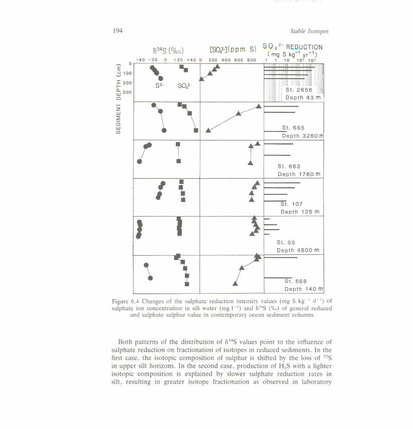
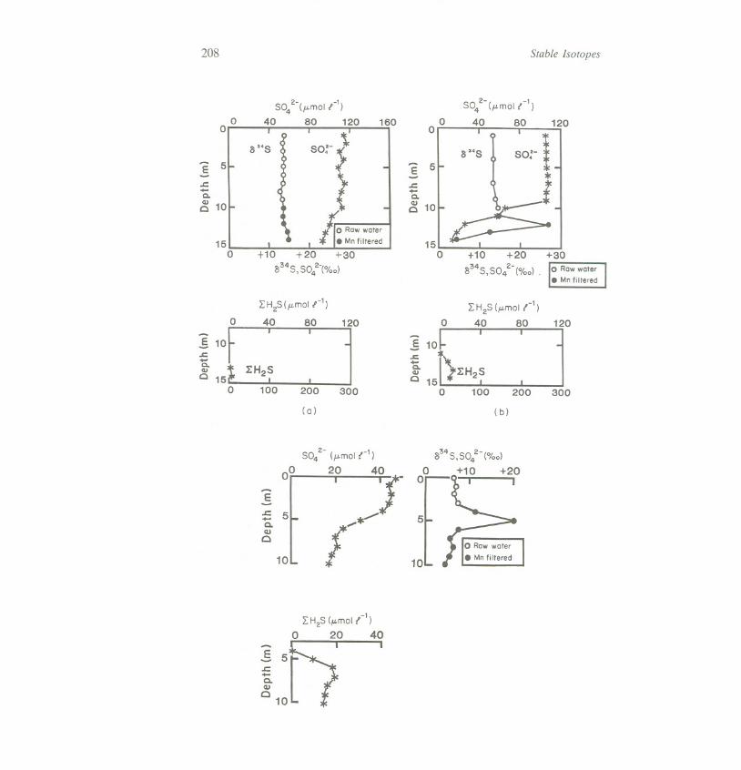
Analysis of dissolved sulphate in silt and total reduced sulphur in columnsof bottom sediments revealed two extreme patterns in sulphur isotopedistribution (Figure 6.4). In sediments with intensive pore water sulphatereduction and poor filtering properties (Figure 6.2, st. 655), the isotopiccompositions of sulphur of pore-water sulphate and total reduced sulphurapproach equality with depth.

In sediments with a constant high SOi- content (Figure 6.2, st. 663),reduced sulphur in lower horizons is appreciably depleted in the heavier34S.

Hydrosphere 193

Table 6.6 Intensity of sulphate reduction, average isotopic composition, productionof reduced sulphur, and organic carbon consumption in oceanic sediments

Production ofArea of Intensity of reduced

sediments SOl- reduction (')34S sulphurRegion and depth (106 km2) (....gS kg-1 d-l) (%0) (Tg yr-l)

Marshes - -17.7 -"

Gulfs, lagoons,estuaries - -16.5 - a

Shelf0--50 m 11 (2)b 55.6 -24.2 79.250--200 m 16 (3) 37.2 53.1

Continental slope200--1000m (15) 28.2 201.0

1000--3000m (61) 5.5 -33.2 158.6Deep-watersediments 257 1.0 -41.1

Total for the ocean 360 (81) 491.9

194

8348 (%0)

Stable Isotopes

[SOlJ(ppm S) SO 42- REDUCTION( mg S k -1 -1

200 400 600 800 .1 1 10 9 10yr10)

St. 668Depth 140 m

Figure 6.4 Changes of the sulphate reduction intensity values (mg S kg-I d-I) ofsulphate ion concentration in silt water (mg I-I) and a34s (0/00)of general reduced

and sulphate sulphur value in contemporary ocean sediment columns

0Eu 100'-'I200I-

fu 3000I-ZW~0w(/) ~

/

J

\

.

1

:"

1

1

/

11 :!I

,iii~~!i:~iw! III~ Depth 43 m

/ ~t. 665 I

Depth 3260 m

!St. 663

Depth 1760 m

I \ {St. 107

Depth 125 m

St. 59

Depth 4800 m

Both patterns of the distribution of 334Svalues point to the influence ofsulphate reduction on fractionation of isotopes in reduced sediments. In thefirst case, the isotopic composition of sulphur is shifted by the loss of 3ZSin upper silt horizons. In the second case, production of HzS with a lighterisotopic composition is explained by slower sulphate reduction rates insilt, resulting in greater isotope fractionation as observed in laboratory

-40 -20 0 +20 +40 0

'- ..82- SOi-

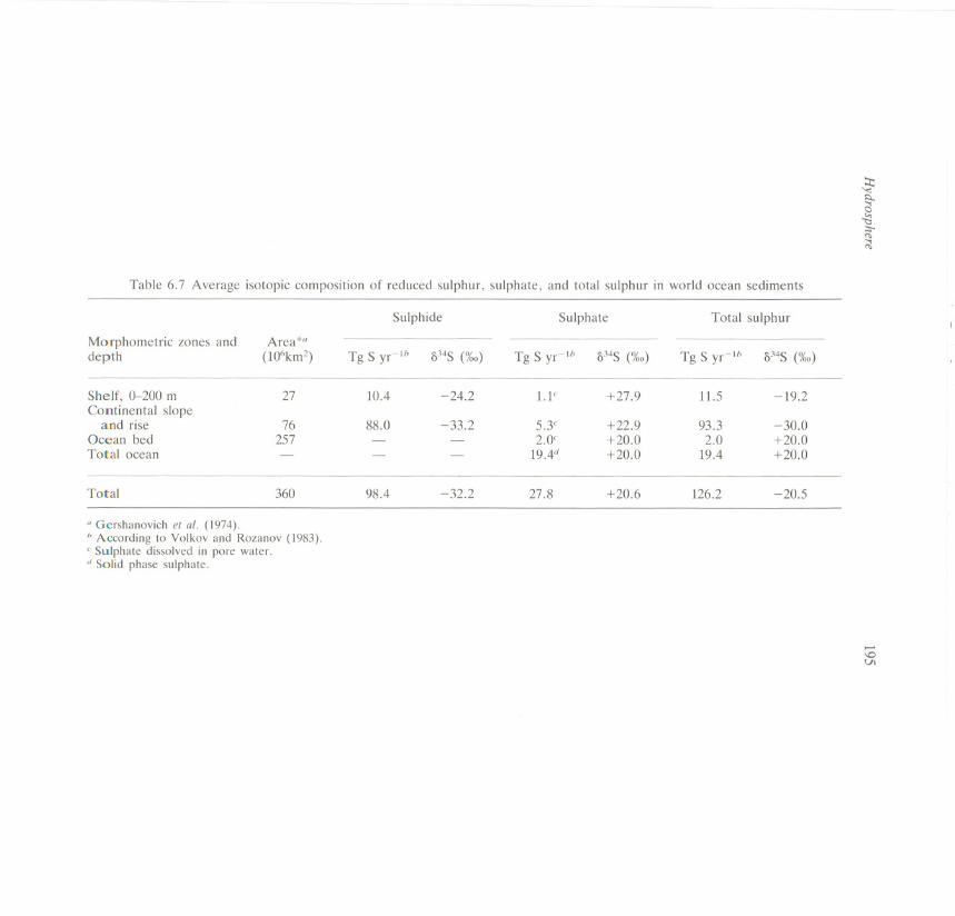
Table 6.7 Average isotopic composition of reduced sulphur, sulphate, and total sulphur in world ocean sediments

Morphometric zones anddepth

Area *a

(106km2)

Sulphide

Tg S yr-1b !)J4S (%0)

Sulphate Total sulphur

Tg S yr-1b !)J4S (%0) Tg S yr-Ib !)J4S (%0)

27Shelf, 0-200 mContinental slope

and riseOcean bedTotal ocean

76257

10.4

88.0

-24.2

-33.2

Total 360 98.4 -32.2

" Gershanovich el al. (1974).h According to Volkov and Rozanov (1983).<' Sulphate dissolved in pore water.

d Solid phase sulphate.

~:::...;j~;:-'"~

>-'\DVI

1.1' +27.9 11.5 -19.2

5.3' +22.9 93.3 -30.02.0" +20.0 2.0 +20.0

19.4<1 +20.0 19.4 +20.0

27.8 +20.6 126.2 -20.5

196 Stable Isotopes

experiments (cf. Jones and Starkey, 1957; Harrison and Thode, 1958; Kaplanand Rittenberg, 1964; Chambers and Trudinger, 1979).

The substantial increase in the fractionation of sulphur isotopes withdecreasing intensity of sulphate reduction is expressed in the ranges of ;)34Sdata for various geomorphological zones of the world ocean system (Table6.6; Figure 6.5). These data are of primary importance since they suggestthat ;)34Svalues of reduced sulphur in rocks may enable an assessment ofthe intensity of sulphate reduction in the geological past.

6.3.3 Mass and isotopic balance of sulphur in recent sediments

Table 6.7 contains data necessary for calculating the material and isotopicsulphur balance in modern oceanic sediments. The total sulphur buriedannually (other than evaporite formation) is estimated to be 126 Tg, withan average ;)34Svalue = -20.5%0. The major portion of sulphur is buriedin reduced forms (primarily pyrite) with an average ;)34Svalue of - 32.2%0.

A comparison of data in Tables 6.6 and 6.7 shows that only 20% of newlyformed hydrogen sulphide is buried as sulphide minerals in sediments,whereas the remainder is internally cycled. H2S migrates to the upper

-40834S (%0)

0 +20 +40

BAL TIC SEA

CONTINENT AL SHELF0-200 m

CONTINENTAL SLOPE200-1000 m200-1000m

1000-3000 m

-20. .SULPHIDE

i &" ~ I""'''

CD ~ ex5hg00

o~fjId3!!

0~8°T 00 0

SULPHATE

SLOPE SEAFLOORTRANSITION ZONE

> 3000 m

.~ 00 'ffi~BBo0 00

0

"'f

~!I!l1SI

&~ ...°t~ 00 0

ot .-B0

~0.

"1 IS!502 .6"3 07.4 +8

OCEANIC TRENCH> 6000 m 0 e~ e 0

RED SEA RIFT +

Figure 6.5 Variations of 8]4Ssulphide and sulphate value in sea and ocean sediments.I-Baltic Sea, 2-South China Sea, 3-California Bay, 4-Tasman Sea, 5-PacificOcean Shelf near Mexico, 6--western part of the transocean geologic section, 7-the area of the Peru upwelling activity, 8-abiogenic sulphides of the active ocean

zones

Hydrosphere

horizons and is oxidized there to sulphate. This is confirmed by maxima inpore-water sulphate concentration just below the surface of the sediments.This sulphate is depleted in 34S (034S = -15.2 to -18.5%0) as comparedwith 21%0 for open-ocean SOi- (Lein et al., 1981). This demonstratesunambiguously the generation of excessive sulphate by the oxidation ofbiogenic hydrogen sulphide (Figure 6.2, s1. 668).

In rare cases where one knows the rate of sedimentation as well as the

total sulphur content and sulphate reduction intensity, it is possible toestimate the portion of reduced sulphur buried in the form of pyrite forindividual sediment horizons (Table 6.8). Values of buried sulphur for twoexamples considered (15 and 16%, Table 6.8) are within the limits acceptedfor global calculations (about 20%, Tables 6.6 and 6.7).

197

6.3.4 Influence of the rate of sulphate reduction on sulphide mineralformation

Sulphide minerals isolated from marine sediments with varying intensitiesof bacterial sulphate reduction are markedly different in composition andmorphology.

Dissolved sulphide and iron sulphide are always present in subcontinentalsediments where there is intensive bacterial sulphate reduction. Sulphideion is easily oxidized chemically and microbiologically (Jannasch et al., 1974;Gorlenko et al., 1977), yielding excess sulphur. Such conditions promoteframboidal pyrite formation.

In sediments with low rates of bacterial reduction, free hydrogen sulphideand sulphide ion are practically absent in pore water. These conditions

Table 6.8 Example of the calculation of sulphide sulphur buried in sediments withknown rate of sedimentation

Baltic Sea, st. 2656,depth 46 m"

Pacific ocean shelfnear Mexico, depth

140 m"--

Horizon of silt (cm)Duration of the process (years)Intensity (mg kg-I d-I)Calculated content (g kg-I)True content (g kg-I)Buried sulphur (% of calculatedvalue)

3.0-4.0355.4

68.010.215

17.5-25750

0.5637.56.016

" Lein et al. (1982).b Ivanov et al. (1976).

198 Stable Isotopes

promote formation of non-framboidal pyrite and pyrite aggregates withsulphide minerals of the mackinawite-greigite group. Therefore, the decreasein sulphate reduction rate evidently inhibits the transformation of unstablesulphide minerals to pyrite.

Sulphides formed from abiogenic hydrogen sulphide in sediments oftectonically active zones of the ocean (Red Sea depressions, East Pacificupwelling, crater lakes, etc.) are represented by individual crystals of cubic,prismatic, and other habits or by drusy and clusterlike aggregates. Suchsulphides are characterized by 534S values in the range -3.0 to +3.0%0,which is radically different from that of sulphides in other regions of theocean (Lein et al., 1982; Lein, 1983).

6.4 LAKES*

6.4.1 Lakes: water column

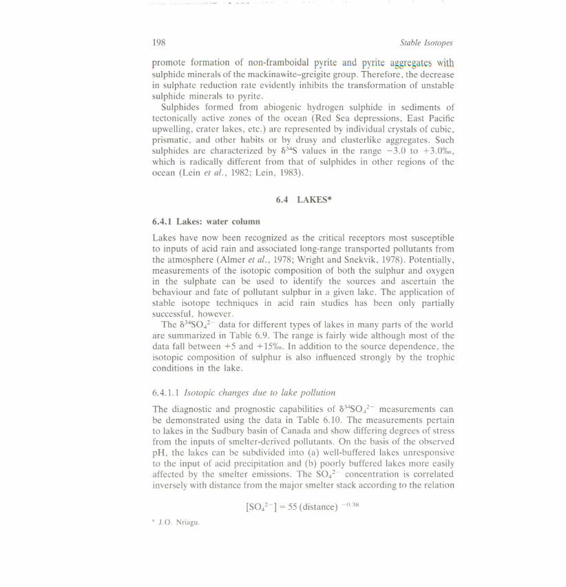
Lakes have now been recognized as the critical receptors most susceptibleto inputs of acid rain and associated long-range transported pollutants fromthe atmosphere (Almer et al., 1978; Wright and Snekvik, 1978). Potentially,measurements of the isotopic composition of both the sulphur and oxygenin the sulphate can be used to identify the sources and ascertain thebehaviour and fate of pollutant sulphur in a given lake. The application ofstable isotope techniques in acid rain studies has been only partiallysuccessful, however.

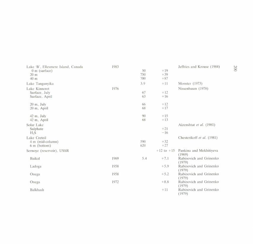
The 534S0i- data for different types of lakes in many parts of the worldare summarized in Table 6.9. The range is fairly wide although most of thedata fall between + 5 and + 15%0.In addition to the source dependence, theisotopic composition of sulphur is also influenced strongly by the trophicconditions in the lake.

6.4. 1.1 Isotopic changes due to lake pollution

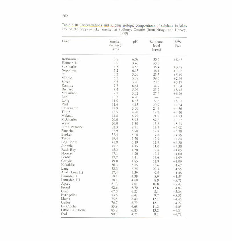
The diagnostic and prognostic capabilities of 534S0i- measurements canbe demonstrated using the data in Table 6.10. The measurements pertainto lakes in the Sudbury basin of Canada and show differing degrees of stressfrom the inputs of smelter-derived pollutants. On the basis of the observedpH, the lakes can be subdivided into (a) well-buffered lakes unresponsiveto the input of acid precipitation and (b) poorly buffered lakes more easilyaffected by the smelter emissions. The SOl- concentration is correlatedinversely with distance from the major smelter stack according to the relation

[SOi-] = 55 (distance) -0.38

* J.O. Nriagu.

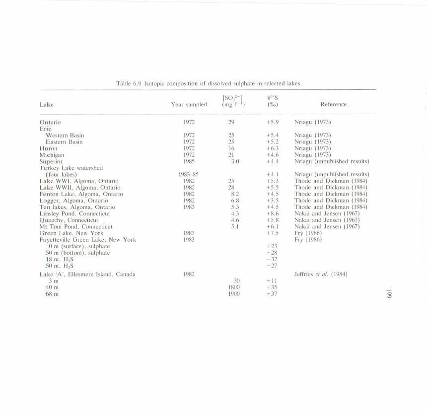
Table 6.9 Isotopic composition of dissolved sulphate in selected lakes

[SO/-] 0:14SLake Year sampled (mg €-') (%0) Reference

--- --- -----

Ontario 1972 29 +5.9 Nriagu (1973)Erie

Western Basin 1972 25 +5.4 Nriagu (1973)Eastern Basin 1972 25 +5.2 Nriagu (1973)

Huron 1972 16 +6.3 Nriagu (1973)Michigan 1972 21 +4.6 Nriagu (1973)Superior 1985 3.0 +4.4 Nriagu (unpublished results)Turkey Lake watershed

(four lakes) 1983-85 +4.1 Nriagu (unpublished results)Lake WWI, Algoma, Ontario 1982 25 +5.3 Thode and Dickman (1984)Lake WWII, Algoma, Ontario 1982 28 +5.5 Thode and Dickman (1984)Fenton Lake, Algoma, Ontario 1982 8.2 +4.5 Thode and Dickman (1984)Logger, Algoma, Ontario 1982 6.8 +3.5 Thode and Dickman (1984)Ten lakes, Algoma, Ontario 1983 5.3 +4.5 Thode and Dickman (1984)Linsley Pond, Connecticut 4.3 +8.6 Nakai and Jensen (1967)Queechy, Connecticut 4.6 +5.8 Nakai and Jensen (1967)Mt Tom Pond, Connecticut 5.1 +6.1 Nakai and Jensen (1967)Green Lake, New York 1983 +7.5 Fry (1986)Fayetteville Green Lake, New York 1983 Fry (1986)

0 m (surface), sulphate +2350 m (bottom), sulphate +2818 m, HzS -3250 m, HzS -27

Lake 'A', Ellesmere Island, Canada 1982 Jeffries et al. (1984)3m 30 +11

40 m 1800 +35 .....68 m 1900 +37

Lake 'B', Ellesmere Island, Canada 1983 Jeffries and Krouse (1984) N0

0 m (surface) 50 +19 020 m 750 +3940 m 700 +87

Lake Tanganyika 3.9 +11 Monster (1973)Lake Kinneret 1976 Nissenbaum (1978)

Surface, July 67 +12Surface, April 63 +16

20 m, July 66 +1220 m, April 68 +17

42 m, July 90 +1542 m, April 68 +13

Solar Lake Aizenshtat et at. (1981)Sulphate +21H2S -16

Lake Creteil Chesterikoff e/ at. (1981)4 m (mid-column) 590 +326 m (bottom) 620 +27

Sernoye (reservoir), USSR + 12 to + 15 Pan kina and Mekhitiyeva(1969)

Baikal 1969 5.4 +7.1 Rabinovich and Grinenko(1979)

Ladoga 1958 +5.9 Rabinovich and Grinenko(1979)

Onega 1958 +5.2 Rabinovich and Grinenko(1979)

Onega 1972 +8.8 Rabinovich and Grinenko(1979)

Balkhash +11 Rabinovich and Grinenko(1979)

Lake

Issyk Kul

Sabundy-KulDzhasybayUI'kenonkol'lPashennoyeShchuch'yeChelbar (brackish)Itkol'Sakovo

2 m, sulphate7 m, sulphate7 m, H2S

Yanda, Antarctica4m

40 m60 m68 m

N0......

Table 6.9 Continued

[S042- 834S

Year sampled (mg £-1) (%0) Reference-- ---------

+15 Rabinovich and Grinenko(1979)

+9.5 Chukhrov et al. (1975)+15 Chukhrov et al. (1975)+13 Chukhrov et al. (1975)+4.4 Chukhrov et al. (1975)+4.4 Chukhrov et al. (1975)+10 Chukhrov et al. (1975)+6.2 Chukhrov et al. (1975)

Matrosov et al. (1975)51 +13

242 +15-11

1973-3 Nakai et al. (1975)8.7 + 1524 +17

237 +22611 +46

202

Table 6.10 Concentrations and sulphur isotopic compositions of sulphate in lakesaround the copper-nickel smelter at Sudbury, Ontario (from Nriagu and Harvey,

1978)

Lake Smelter pH Sulphate 834Sdistance level (%0)

(km) (ppm)

Robinson L. 3.2 6.09 30.5 +8.46Hannah L. 3.9 3.40 53.0St Charles 4.5 4.53 35.4 +3.48Nepohwin 5.2 6.15 36.1 +7.32'e' 5.2 3.20 23.5 +5.19Middle 5.2 5.78 39.5 +2.66Silver 6.5 3.20 28.5 +5.19Ramsay 7.7 6.61 34.7 +7.34Richard 8.4 5.06 25.7 +8.43McFarlane 9.7 5.32 27.4 +6.76Lohi 10.3 4.20 -Long 11.0 6.45 22.3 +5.31Raft 11.6 4.15 20.9 +2.84Clearwater 12.9 3.50 24.4 +4.56Tilton 13.5 4.20 19.3 +4.50Makada 14.8 6.75 21.8 +4.23McCharies 20.0 8.95 87.8 +3.57Wavy 20.0 3.30 15.8 +5.23Little Panache 32.3 8.71 13.7 +6.08Panache 32.9 6.70 19.9 +4.70Broker 37.4 5.20 7.8 +4.75Tyson 39.4 5.70 12.9 +4.84Log Boom 41.9 5.19 12.9 +4.80Johnnie 45.2 4.15 11.0 +4.30Ruth-Roy 45.2 4.50 12.8 +4.05Norway 47.1 4.20 12.3 +4.00Perdix 47.7 4.41 14.6 +4.99Carlyle 49.0 4.85 11.9 +4.99Kakakise 50.3 5.75 13.6 +4.67Lang 52.3 6.75 20.3 +4.55Acid (Lum II) 57.4 4.39 9.5 +4.48Lumsden I 58.1 4.39 8.9 +4.55Lumsden III 58.1 4.60 8.9 +5.71Apsey 61.3 7.01 10.8 +5.43Frood 62.6 6.70 17.6 +4.82Grab 67.0 6.25 8.1 +5.26Evangeline 73.6 6.42 9.7 +5.36Maple 75.5 6.40 12.1 +4.46Cutler 76.7 6.79 12.1 +4.22La Cloche 83.9 6.68 11.2 +5.03Little La Cloche 85.8 6.80 13.2 +4.34Owl 90.3 4.75 8.1 +4.73

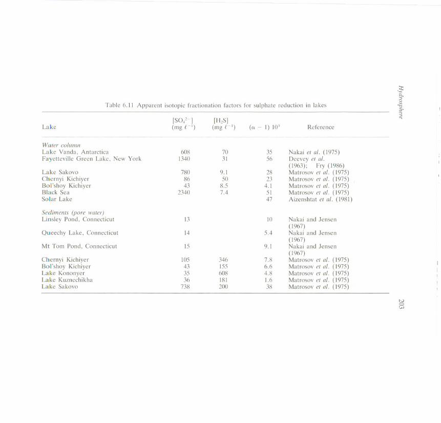
Table 6.11 Apparent isotopic fractionation factors for sulphate reduction in lakes

Lake[S042-](mg {H)

[H2S](mg £-1)

- -~-- -- .--

Water columnLake Yanda, AntarcticaFayetteville Green Lake, New York

Lake SakovoChernyi KichiyerBol'shoy KichiyerBlack SeaSolar Lake

Sediments (pore water)Linsley Pond, Connecticut 13

Queechy Lake, Connecticut 14

Mt Tom Pond, Connecticut 15

105433536

738

346155608181200

Chernyi KichiyerBol'shoy KichiyerLake KononyerLake KuznechikhaLake Sakovo

(ex- 1) 10-'

2823

4.15147

5.4

9.1

7.86.64.81.638

Reference--~ --~

3556

Nakai et al. (1975)Deevey et al.(1963); Fry (1986)Matrosov et al. (1975)Matrosov et al. (1975)Matrosov et al. (1975)Matrosov et al. (1975)Aizenshtat et al. (1981)

10 Nakai and Jensen( 1967)Nakai and Jensen(1967)Nakai and Jensen(1967)Matrosov et al. (1975)Matrosov et al. (1975)Matrosov et al. (1975)Matrosov et al. (1975)Matrosov et al. (1975)

~:::...

(S~:::-'"~

N0w

608 701340 31

780 9.186 5043 8.5

2340 7.4

204 Stable Isotopes

with r = 0.81 (Nriagu and Harvey, 1978). There is also a significantcorrelation between the pH of poorly buffered lakes and the distances fromthe smelter stack. The 034S0/- for the well-buffered lakes show considerablescatter (see Fig. 3 in Nriagu and Harvey, 1978), suggesting (a) derivationof the sulphur from several sources and/or (b) complex interplay betweenthe point source influence and sulphur transformations either in the watershedor within the lakes. For example, high acid loading may increase the amountof sulphur in these lakes by accelerating the weathering of the bedrock andthe overburden. By contrast, the 034S042- data for the poorly bufferedlakes are remarkably uniform, lying mostly between +4 and +5.5%0 (Table6.10). This uniformity clearly suggests that the isotopic composition of theselakes is regulated by the influx of sulphur released from the smelters.

In the Great Lakes system of North America, anthropogenic sources nowaccount for 30% of the SO/- in Lakes Superior and Huron and over 70%in Lake Erie (Nriagu, 1984). There is some suggestion that the industrialinputs are affecting the isotopic composition of SO/- (Table 6.9), althoughthe inter-lake differences do not seem to be consistent with the levels of

pollution. Lake Superior, in particular, has a long water flushing time (about180 years) and thus contains some sulphur of precolonial age. Like the otherGreat Lakes, Superior has a small watershed-to-lake area ratio, implyingthat direct atmospheric deposition accounts for a large fraction of the sulphurinput. Its 034S0/- can thus be regarded as being representative of'unpolluted' waters of the Great Lakes. As can be seen in Table 6.11, the034S0/- data for the other Great Lakes with more pollutant sulphur deviatefrom this background value significantly.

The stable isotope technique has been used with some success to assessthe contamination of surface waters with sulphur emissions from sour gasprocessing plants at West Whitecourt, Alberta (Krouse et al., 1984). Itwas found that the dissolved sulphur became heavier with increasingorganosulphur content. The 034S approached a limiting value of + 22%0(Figure 6.6), which corresponded to the isotopic composition of the sulphurreleased from the sour gas plants. The results of the study suggest that theemission were affecting the biological uptake of sulphur in the borealforest, which in turn resulted in a marked increase in the flux of isotopicallylabelled organosulphur compounds into the surface waters (Krouse et al.,1984).

6.4.1. 2 Oligotrophic lakes

With the exception of Lake Erie, the Great Lakes of North America possessa characteristic feature of oligotrophic lakes, namely very homogeneousisotopic composition of sulphate. Differences in mean 034S0/~ values ofthe hypolimnion and epilimnion waters were generally less than 0.2%0

Hydrosphere 205

+20

-0~~,OJ

0" I(/) I

- +101>'"

(.()

00 10 20

DISSOLVEDORGANICSULPHUR(JLgr')Figure 6.6 The 1)34Svalues for total dissolvedsulphur in water versusorganicsulphurconcentration in selectedwater samplesfromthe WestWhitecourtstudy area (Krouse

et al., 1984)

(Nriagu, 1973). Temperature (seasonal) changes apparently do not promotesignificant sulphur isotope fractionation; nor does assimilatory sulphatereduction by biota.

For many hardwater and/or softwatwer oligotrophic lakes, the 034S0i-values are very close to those of rainfall in their drainage basins, implyinga common origin. Good examples are the Algoma Lakes (including thoseof the Turkey Lakes Watershed) of northern Ontario (Table 6.9). For manyhardwater lakes of oligotrophic classification, the 034S0i- values reflectthe combined signatures of sulphur from atmospheric fallout and from theweathering of the bedrocks. As noted already, most of the poorly bufferedlakes in the Sudbury basin fall into this category.

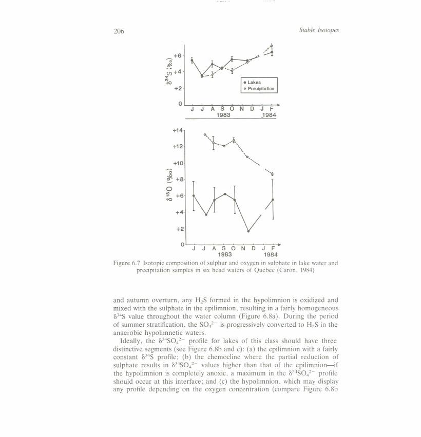
Recent studies of the isotopic composition of oxygen of the dissolvedsulphate in oligotrophic lakes have yielded unexpected results (Caron, 1984;Fritz et al., 1986). The 0180 values of SOi- tend to be distinctly differentfrom those of rainfall and often show complex patterns unrelated to the034S data (Figure 6.7). The oxygen isotopic data thus point to extensiveassimilatory reduction of sulphate, and suggest that the turnover of sulphurin oligotrophic lakes may be more rapid than has hitherto been realized.

6.4.1. 3 Eutrophic lakes

The S042-, HzS, and ()34S0l- profiles in a typical eutrophic lake thatdevelops an anoxic hypolimnion are shown in Figure 6.8. During the spring

206 Stable Isotopes

~+60

"g~U)+4

.,.Jt)(;()

+2

0J J A SON D J F

1983 1984.'-----+14

+12

o.." t /~",...' ","

'",", "+10

0

c¥- +8

0~ +6'0

"-'§

+4 ~+2

0 JJASONDJF1983 1984

Figure 6.7 Isotopic composition of sulphur and oxygen in sulphate in lake water andprecipitation samples in six head waters of Quebec (Caron, 1984)

and autumn overturn, any HzS formed in the hypolimnion is oxidized andmixed with the sulphate in the epilimnion, resulting in a fairly homogeneous034Svalue throughout the water column (Figure 6.8a). During the periodof summer stratification, the SO/- is progressively converted to HzS in theanaerobic hypolimnetic waters.

Ideally, the 034S0/- profile for lakes of this class should have threedistinctive segments (see Figure 6.8b and c): (a) the epilimnion with a fairlyconstant 034S profile; (b) the chemocline where the partial reduction ofsulphate results in o34S0/- values higher than that of the epilimnion-ifthe hypolimnion is completely anoxic, a maximum in the 034S04Z- profileshould occur at this interface; and (c) the hypolimnion, which may displayany profile depending on the oxygen concentration (compare Figure 6.8b

Hydrosphere 207

and c). If the system is completely anoxic, there is a severe shortage ofsulphate and relatively little fractionation of the sulphur isotopes is expected.If the system is partly anoxic (due to leakage of oxygen across thechemocline), the 034S0i- should increase towards the sediment-waterinterface, in accordance with gradients of declining redox potential andincreasing intensity of sulphate reduction. These two may be regarded asthe ideal profiles. Many factors, however, can modify the 034S0i- profilesin the hypolimnion, such as (a) the thickness of the hypolimnion and theduration of stratification, (b) the sulphate concentration and internalbiogeochemical processes in the water column, and (c) the exchange ofsulphur isotopes across the sediment-water interface (Nriagu and Soon,1985). If a large fraction of the product HzS is removed to the sedimentsby reaction with Fez+, the 034S0i- data in the anoxic hypolimnion mayeven show measurable seasonal changes.

In view of the many compounding variables, few, if any, good modelshave been developed to describe the fractionation of sulphur isotopes inthis lake type. It should be noted that few studies have included themeasurement of the isotopic composition of the oxygen in the sulphate.

6.4.1.4 Meromictic lakes

These differ from the eutrophic lakes in (a) being permanently stratifiedand (b) generally having a higher concentration of dissolved salts. Typical034S0i- profiles in meromictic lakes can also be expected to show threedistinct segments corresponding to the epilimnion, chemocline, and monimo-limnion. Representative profiles are shown in Figure 6.9. In FayettevilleGreen Lake, State of New York, the 034S0i- value is essentially constantnear +23%0 in the epilimnion (1-15 m), but increases gradually with depthdown the monimolimnion. As expected, the reduced sulphur species weredepleted in 34Sand the isotopic difference between the SO i- and HS- waslarge and remarkably constant at about 56.6%0 (Deevey et al., 1963; Fry,1986). By contrast, the profile of 034S0i- in Lake Yanda, Antarctica,shows a sharp increase at a depth of 60 m below the ice cover where theHzS becomes detectable. The maximum value of +49%0 was attained rightat the sediment-water interface (Figure 6.9). The sharp increase in sulphateconcentration occurs at about 10 metres above the point of rapid increasein o34S0i- values (Nakai et al., 1975).

Figure 6.8(a) 534S0/-, SO/-, and total dissolved sulphide profiles in Lake 223 on15 June 1979, or following the spring overturn (Cook, 1981). (b) 5'4S0/-, SO/-,and total dissolved sulphate profiles in Lake 223 on 21 September 1979, or duringstratification (Cook, 1981). (c) 534S042-, SO/-, and total dissolved sulphate profiles

in Lake 227 on 1 September 1978, or during stratification (Cook, 1981)

208

~ 5~.....Q.IV

C 10

15-0

0

~ 10f"S. '\'~ 15i!:.

0

00

2- -15°4 (fLmoll )

40 80 120 160

80:- { ,

t[;w w.."I I f I~ Mnfiltered+10 + 20 +30

8345,50t(%0)

8 "8

2: H25 (fLmol r1)

::]0100200(0 )

300

00

5042- (fLmoi r1)

2~ 40)

f~*/

E

-12: H25 (fLmol ( )

0 20 40

i5~ '~j {

Stable Isotopes

-12:H25 (fLmol t )

1::&<": ~O J0 100 200 300

( b)

8345,5°42- (%0)0 +10 +20

Or-Q I I

5

10

0 40 80 12001 I

. o:-l

-l \.§. *

i210

151 I I0 +10 +20 +30

8345,5042- (%0) .

Hydrosphere209

8348 (%0)-34 -30 -26 +22

0 I Fayett~ville Gr~en -r.ak~.'New York j

+26 +30

] 20.s::C.Q)c 40 ~

60

00

+208348 (%0)

-I- 40 + 60 +80

20

180:-1

]-5 40a.Q)C

60

80

Figure 6.9 Profiles of sulphur isotopes in typical meromictic lakes (data forFayetteville Green Lake from Fry, 1986, for Lake Yanda from Nakai et al., 1975,

and for 'A' Lake from Jeffries et al., 1984)

The sulphate concentration in Lake 'A', Ellesmere Island in the CanadianArctic, increases from about 30 mg €-l just below the ice cover to well over1900 mg €-l in the bottom waters (Jeffries et ai., 1984). The 034S0i- andoU'O-S042- also increase with depth from the ice cover although samplesclosest to the sediments are slightly depleted in 34S. The isotopic profilesdo not depict the freshwater-to-seawater transition zone located at depthsof 15-25 metres.

In the case of smaller Lake 'B', which is slightly further inland, Jeffriesand Krouse (1984) found the 034Svalues of bottomwater S042- to be ashigh as +87%0 (Figure 6.7). Dissolved carbonate in the bottom waters had034C values of - 21 and - 27%0for Lakes A and B respectively, which is inthe range of organic matter. In summary, the sulphur, oxygen, and carbonisotope data collectively provide strong evidence of anaerobic bacterialS042- reduction with attending oxidation of organic nutrients. Because of

210 Stable Isotopes

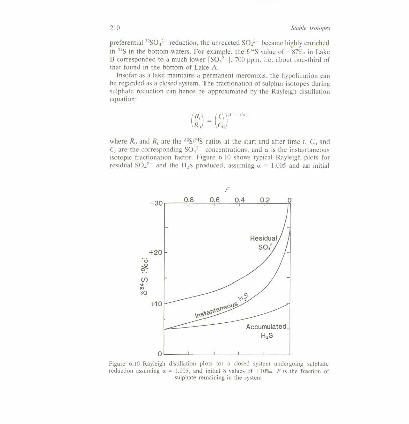
preferential 3zS0i- reduction, the unreacted S04z- became highly enrichedin 34S in the bottom waters. For example, the 034Svalue of +87%0 in LakeB corresponded to a much lower [S04Z-], 700 ppm, i.e. about one-third ofthat found in the bottom of Lake A.

Insofar as a lake maintains a permanent meromixis, the hypolimnion canbe regarded as a closed system. The fractionation of sulphur isotopes duringsulphate reduction can hence be approximated by the Rayleigh distillationequation:

(Rt

)=

(C

)

(1 - l/a)

Ro Co

where Ro and Rt are the 3ZSp4S ratios at the start and after time t, Co andC are the corresponding SO/- concentrations, and (Xis the instantaneousisotopic fractionation factor. Figure 6.10 shows typical Rayleigh plots forresidual S04Z~ and the HzS produced, assuming (X= 1.005 and an initial

F

+30 0.8 0.6 0.4 0.2

AccumulatedH2S

0

Figure 6.10 Rayleigh distillation plots for a closed system undergoing sulphatereduction assuming ex= 1.005, and initial 0 values of +10%0. F is the fraction of

sulphate remaining in the system

+200

0

(f)<tr<)ro

+10

Hydrosphere 211

834S0i- of + 10%0.The patterns of the calculated graphs generally matchwhat have been observed in some meromictic lakes (compare Figures 6.9and 6.10).

Values of a for sulphate reduction in lake waters and sediments rangefrom 1.004 to 1.056 (Table 6.11). As to be expected, the lowest a valuesare found in lakes with the lowest sulphate concentrations-the sulphatereducers become less discriminating as the available sulphate is depleted. Italso means that in lakes with low SOi- content, the value a is not constantbut will decrease as the available sulphate is biotransformed into reducedspecies. The available data suggest that when the sulphate concentration isless than 20 mg £-1, the value of a is generally below 1.01. In contrast, ais much larger (1.03-1.07) in marine environments with abundant S042-(Goldhaber and Kaplan, 1974). It is not surprising that some of the a valuesfor lakes fall in the marine range, considering their sulphate concentrations(Table 6.11).

6.4.2 Lakes: sediments

A detailed review of the distribution and diagenesis of sulphur in lacustrinesediments has already been given in a preceding SCOPE volume (Ivanovand Freney, 1983). The monograph includes a good summary on the use ofsulphur isotopes in delineating the critical pathways of sulphur transformationsin sediment ecosystems. To avoid duplication, the following sectionconcentrates on the use of stable sulphur isotopes in understanding freshwatersediments as sinks for anthropogenic sulphur, especially in eastern NorthAmerica. The reduction of anthropogenic sulphate in lake sediments is animportant alkalinity-generating process. Measurements of the isotopiccomposition of sulphur in sediments can thus (a) provide some insight onthe self-purification of a lake and its ability to recover from an acid stressand (b) be used for retrospective monitoring of past fluxes of pollutantsulphur into the lake basin. These are key questions relevant to acid rain.

6.4.2.1 Anthropogenic influence on the isotopic composition of sulphur inlake sediments of eastern North America

The role of lake sediments as sinks for pollutant sulphur has received littleattention. Several studies have now demonstrated that there has been asignificant increase in the sulphur contents of the most recent sediments oflakes in many parts of the world (Table 6.12). For example, the enrichmentfactors (EF) for the Great Lakes vary from about 1.5 in the fairly pristineLake Superior to over 3 in the most polluted, much shallower, Lake Erie.(EF is the ratio of the average S concentration in surficial sediments to thatin the precolonial layers. The difference between the S contents of the two

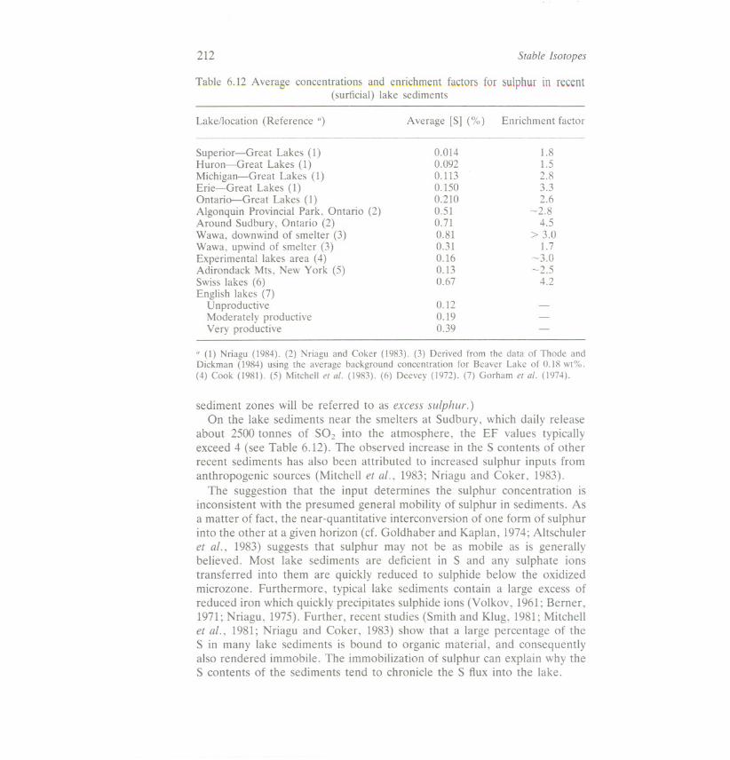
212 Stable Isotopes

Table 6.12 Average concentrations and enrichment factorsfor sulphur in recent(surficial) lake sediments

Lake/location (Reference a) Enrichment factorAverage [S] (%)

Superior-Great Lakes (1)Huron-Great Lakes (1)Michigan-Great Lakes (1)Erie-Great Lakes (1)Ontario-Great Lakes (1)Algonquin Provincial Park, Ontario (2)Around Sudbury, Ontario (2)Wawa, downwind of smelter (3)Wawa, upwind of smelter (3)Experimental lakes area (4)Adirondack Mts, New York (5)Swiss lakes (6)English lakes (7)

UnproductiveModerately productiveVery productive

0.0140.0920.1130.1500.2100.510.710.810.310.160.130.67

1.81.52.83.32.6

-2.84.5

> 3.01.7

-3.0-2.5

4.2

0.120.190.39

a (1) Nriagu (1984). (2) Nriagu and Coker (1983). (3) Derived from the data of Thode andDickman (1984) using the average background concentration for Beaver Lake of 0.18 wt%.(4) Cook (1981). (5) Mitchell et at. (1983). (6) Deevey (1972). (7) Gorham et al. (1974).

sediment zones will be referred to as excess sulphur.)On the lake sediments near the smelters at Sudbury, which daily release

about 2500 tonnes of S02 into the atmosphere, the EF values typicallyexceed 4 (see Table 6.12). The observed increase in the S contents of otherrecent sediments has also been attributed to increased sulphur inputs fromanthropogenic sources (Mitchell et al., 1983; Nriagu and Coker, 1983).

The suggestion that the input determines the sulphur concentration isinconsistent with the presumed general mobility of sulphur in sediments. Asa matter of fact, the near-quantitative interconversion of one form of sulphurinto the other at a given horizon (d. Goldhaber and Kaplan, 1974; Altschuleret al., 1983) suggests that sulphur may not be as mobile as is generallybelieved. Most lake sediments are deficient in S and any sulphate ionstransferred into them are quickly reduced to sulphide below the oxidizedmicrozone. Furthermore, typical lake sediments contain a large excess ofreduced iron which quickly precipitates sulphide ions (Volkov, 1961; Berner,1971; Nriagu, 1975). Further, recent studies (Smith and Klug, 1981; Mitchellet al., 1981; Nriagu and Coker, 1983) show that a large percentage of theS in many lake sediments is bound to organic material, and consequentlyalso rendered immobile. The immobilization of sulphur can explain why theS contents of the sediments tend to chronicle the S flux into the lake.

Hydrosphere 213

The influence of inputs on sedimentary sulphur is further demonstratedby the strong correlation between the S contents of recent sediments andthe sulphate concentrations in the overlying waters (Gorham et at., 1974;Nriagu, 1984). It should be emphasized that the source influence can bestbe seen in lakes with aerobic hypolimnion. Any development of bottomanoxia increases the transfer of S to the sediments, thereby confusing therelationship between sulphur input and accumulation in the sediments.

In fact, the pollution component of S042- in the Great Lakes can beestimated using the shift in the S contents of the sediments. Such data forLake Erie sediments suggest that anthropogenic sources account for about70% (18 mg £-1) of SOi- (Nriagu, 1984). The extrapolation of the historicalgraph of changes in SOi- concentrations (in the overlying water) to precolonialtimes shows a similar pollution input (Beeton, 1965;Pringle et at., 1981).A massbalance of the inputs from the weathering of the bedrocks and the glacialoverburdens likewise suggests that 60-70% of the SOi- in Lake Erie comesfrom pollution sources (Nriagu, 1975). On the basis of the excess sulphur values,it has also been estimated that anthropogenic sources now account for about30-40% of the SOi- in the waters of Lakes Huron and Superior, and about60% in Lake Ontario and southern Lake Michigan. These percentages arein good agreement with the estimated background of precolonial SO/-concentrations of 14 mg £-1 in Lake Ontario, 5 mg £-1 in Lake Michigan,8 mg £-1 in Lake Huron, and 2 mg £-1 in Lake Superior (Beeton, 1965;Pringle et at., 1981).

Potentially, the isotopic technique should provide a confirmation as towhether the sources of S in the recent lake sediments have indeed changed.In one of the first detailed studies, Nriagu and Coker (1976) showed thatthe surficial sediments of Lake Ontario are depleted in 34Scompared to theolder sediments. They interpreted the 334S profiles in terms of sulphurdiagenesis and preferential loss of 32Sto the overlying water; the interpretationwas adapted from diagenetic models for S in marine sediments. A recentstudy of sediments as sinks for S in the Great Lakes (Nriagu, 1984) suggests,in fact, that the observed 334Sprofiles are more likely to be a reflection ofincreasing input of pollutant sulphur into Lake Ontario.

Subsequently, the isotopic composition of S in the humic acids (HA) fromLake Ontario has been determined (Figure 6.11). What is remarkable is thedepletion of 34S in the surficial samples and the close similarity with the334S profiles of the other forms of sulphur in these sediments (see Nriaguand Coker, 1976). The 334S of the HA presumably includes the isotopicsignature of the precursor organic matter, the isotopic imprints of thesubsequent diagenetic changes, and the isotopic effects of any secondaryenrichment reactions (Nissenbaum and Kaplan, 1972; Dinur et at., 1980). Itis impossible to establish the relative influence of each of these threeprocesses. In view of the little that is currently known about the fractionation

214 Stable Isotopes

+50

0345, D/..)+10 +15 0

0+5

034S,(%O)+10 +15

~Qj.c~ 2015.Q)

0

10E.8. 10Q)0

~....Q)

:5 CENTRAL BASIN KINGSTON

(Eastern)BASIN

20

30 30

Figure 6.11 The 034Sprofiles for humic acid sulphur from Lake Ontario

of S isotopes in organic material, it would be ill advised to attribute theshift in isotopic composition solely to a change in the source of the sulphurin the humic acids. Nevertheless, the profile observed is very suggestive ofa strong source influence. It may be noted that the HA is depleted in 34Sin relation to the acid volatile sulphides and the total S in the same sedimenthorizons.

A more recent study dealt with the concentration and isotopic com-position of S in lake sediments located in two contrasting regions withrespect to sulphur pollution. The first group of lakes is located near Sudbury,Ontario, and derives most of the sulphur from the big nickel-copper smeltingcomplex nearby (Nriagu and Coker, 1978a; Nriagu and Harvey, 1978). Thispoint source has a fairly constant isotopic signature and the sedimentaryrecord of sulphur pollution in these lakes should be related to the localhistory of smelting activities. The strong influence of smelter emissions ismanifested by the fact that many of the lakes in this area have becomeacidic (OME, 1981). The second group of lakes are located in the moreremote Algonquin Provincial Park with no known major local sources ofsulphur. The historical records and isotopic profiles in the sediments should

Hydrosphere 215

presumably reflect the flux of long-range transported sulphur into the lakebasins.

Representative profiles of total sulphur and 334Sin lake sediments in thetwo areas are shown in Figure 6.12. A prominent feature of the profiles isthe spectacular enrichment of sulphur in the surficial sediments. For thelakes around Sudbury, the dramatic increase in the flux of excess sulphurbegan around 1890, coinciding with the initiation of smelting operations(Nriagu et at., 1982). It is interesting that the pronounced increase in theaccumulation of S in Windy Lake sediments, located about 20 km fromSudbury, dates to roughly 45 years BP, and hence coincides with theinstallation of the taller 170 m stack at Copper Cliff in 1923. The accumulationof excess S in lake sediments in the Algonquin Park generally began around1860-70, and may be related to the beginning of extensive industrializationof the Great Lakes basin. These data thus suggest that lake sediments aresensitive to the influx of pollutant sulphur from both local and distantsources.

The changes in the 334Sprofiles closely parallel the input of excess sulphurinto the lake sediments (Figure 6.12). Typically, the most recently depositedsulphur is isotopically lighter than the sulphur in the older sediments. Moreimportantly, the shift in 334Scoincides with the onset of excess S in everycase (Figure 6.12). The sulphur in the surficial sediments near Sudburytends to be lighter (average 334S value, ~-8%0) than in Algonquin Parksediments of comparable age (mean 334S value ~-0.5%0). The apparentdifference may be related to the disparity in the isotopic signature of sulphurfrom local versus regional sources (Nriagu and Coker, 1983). The highlycontaminated sediments of Kelly Lake (a recipient of both domestic andindustrial effluents) contain over 3% sulphur with very negative 334Svaluesof -20 to -30%0 (Figure 6.12).

Various diagenetic models, conceivably, can be invoked to account forthe total S or 334Sprofiles. The time frame for the onset of excess sulphuraccumulation in these lakes, however, lends support to their interpretationin terms of input control. The results do suggest that sedimentary sulphurcan be used as a time tracer for acid rain deposition in these lakes. Thequantification of the historical changes in the flux of acidic sulphur compoundsinto lakes would require a careful assessment of principal pathways ofsulphur flux into the sediments. There are currently few reliable indices ofpast changes in the buffering capacity of lakes which can be attributed toacidic precipitation, and the sulphur isotopic technique does seem to providethe much-needed clues.

A few other studies have addressed the 334S profiles in recent lakesediments. The total S content and 334Sprofiles which Cook (1981) reportedin the Experimental Lakes Area of northern Ontario are very similar tothose in Figure 6.12. The total S profiles in two lakes in the Adirondack

216

0TOTAL S (Dry wi %)

1 2

E 0 I -30.gw()

L£ 5ex:w

~10w

j!:::: 159wIn

-25 -20 -15

i!:a.UJQ

Kelly Lake

034S(%")-10 -5

Stable Isotopes

TOTAL S (Dry wi '.IiI)0.2 0.4 0.6 0.8

I I

0

..

LohiLake

0TOTALS (Drywt ,,)

0.2 0.4 0.6 0.6

] 10,w0L£ 20ex:w

!z;;:;30J::I-

~40J

wInJ:: SQ.I-a.wQ 60,

Figure 6.12 Profiles of total sulphur and o34Sin sediments of representative lakesof Northern Ontario (Nriagu and Coker, 1983)

Mcfarlane Lake

4034S(

0

-10 %.,)0

E.g1O-w0L£ex: 20UJ

w30

j!:

40..:.J

i!:50a.

60

70

Hydrosphere 217

Mountains of New York likewise show an increasing flux of excess sulphurbeginning around 1850 (Mitchell et at., 1983); the preliminary datafurthermore show a depletion of 34S in the surficial sediments samples(M.J. Mitchell, personal communication, 1983). Thode and Dickman (1983)found the difference in 034Svalues between the recent and the underlyingolder sediments to be about 3%0and 9-11%0in lakes located downwind andupwind respectively of the smelters at Wawa, Ontario. In each instance, the034Swas shifted to a lower value in the surficial sediments. These availabledata, all from lakes in eastern North America, show a very diagnosticpattern which needs to be confirmed in lakes in the other parts of the world.

6.5 ISOTOPIC COMPOSITION OF SULPHUR IN CONTINENTALSEAS*

In contrast to the world's oceans, concentration and 034Svalues of sulphatein continental seas vary widely. Isotopic data for different sulphur forms inwater and sediments of continental seas are rather sparse even forthe largest, the Mediterranean Sea. The Black Sea has been studiedcomprehensively; less information has been obtained for the Azov, Caspian,Baltic, and Red Seas.

From the environmental viewpoint, inland seas may serve as the recipientsof anthropogenic sulphur. Alternatively, non-sulphur-containing pollutantsmight alter the sulphur cycle in these waters, perhaps affecting biota andemission of S compounds to the atmosphere.

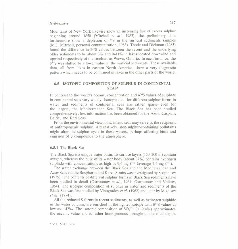
6.5.1 The Black Sea

The Black Sea is a unique water basin. Its surface layers (150-200 m) containoxygen, whereas the bulk of its water body (about 87%) contains hydrogensulphide with concentrations as high as 9.6 mg e-l (average 7.6 mg e-I).

The water exchange between the Black Sea and the Mediterranean andAzov Seas via the Bosphorus and Kerch Straits was investigated by Scopintsev(1975). The contents of different sulphur forms in Black Sea sediments havebeen studied in detail (Ostroumov et at., 1961; Ostroumov and Volkov,1964). The isotopic composition of sulphur in water and sediments of theBlack Sea was first studied by Vinogradov et at. (1962) and later by Migdisovet at. (1974).

All the reduced S forms in recent sediments, as well as hydrogen sulphidein the water column, are enriched in the lighter isotope with 034Svalues aslow as -42%0. The isotopic composition of SO/- (+ 19.4%0)approximatesthe oceanic value and is rather homogeneous throughout the total depth.

* V.L. Mekhtiyeva.

218 Stable Isotopes

Some variations in the isotopic composition of SOl- (from +16.7 to+21.2%0) are observed in the littoral zone (Mekhtiyeva and Pankina, 1968;Chukhrov et al., 1975). The isotopic composition of sulphate in the riversystem of the Black Sea Basin was investigated by Rabinovich and Grinenko(1979).

From data on the contents of different sulphur forms in sediments andthe annual sediment deposition rate on the shelf (145 Tg yr-l), the annualreduced sulphur flux to the Black Sea sediments has been estimated to be2.4 Tg, of which 1.4 Tg reaches the shelf (Lein and Ivanov, 1983). Lein etal. (1983) have calculated the mass isotopic balance for sediments in thehydrogen sulphide zone of the sea.

On the basis of the above data, a mass isotopic balance calculation forsulphur in the entire Black Sea has been attempted (Tables 6.13 and 6.14).

As seen from Table 6.13, the isotopically light sulphur is buried insediments. Despite the fact that this flux is relatively small, it establishes

Table 6.13 Flux of sulphur in the Black Sea sediments

Average S S-ftuxcontent (l0f> tonnesSediment (%) /)J4S(%0) yr-I)

deposition(106 tonnes

Zone yr-I) HzS SO/- HzS SO/- HzS SO/-

Hydrogensulphide 75 1.35 0.03 -23.9 25.6 1.01 0.02

Oxygen 145 1.01 0.05 20.0 23.0 1.46 0.07

Table 6.14 Mass isotopic balance of sulphur in the Black Sea

106 tonnes /)J4S I 106 tonnes /)J4SInputs yr-I ('roo) ! Outputs yr-I ('roo)

River runoff 3.8 +4.5 Efflux to 14.98 +19.0Azov Sea

Flux from the 16.5 +17.0 Efflux to 159.9 + 19.4Azov Sea Bosporus

Flux from 158.7 +19.8 : Burial in 2.47 -20.0Bosphorus sediments

Total 179 +19.2 i 177 -18.8i

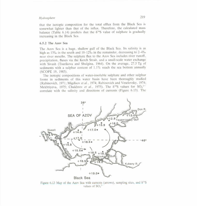
Hydrosphere 219

that the isotopic composition for the total efflux from the Black Sea issomewhat lighter than that of the influx. Therefore, the calculated massbalance (Table 6.14) predicts that the 834S value of sulphate is graduallyincreasing in the Black Sea.

6.5.2 The Azov Sea

The Azov Sea is a huge, shallow gulf of the Black Sea. Its salinity is ashigh as 13%0in the south and 10-12%0in the remainder, decreasing to 2-4%0near river mouths. The sulphate flux to the Azov Sea includes river runoff,precipitation, fluxes via the Kerch Strait, and a small-scale water exchangewith Sivash (Tsurikova and Shulgina, 1964). On the average, 27.5 Tg ofsediments with a sulphur content of 1.1% reach the sea bottom annually(SCOPE 19, 1983).

The isotopic compositions of water-insoluble sulphate and other sulphurforms in sediments of this water basin have been thoroughly studied(Rabinovich, 1971; Migdisov et al., 1974; Rabinovich and Veselovsky, 1974;Mekhtiyeva, 1975; Chukhrov et al., 1975). The 834S values for S042-correlate with the salinity and directions of currents (Figure 6.13). The

360I

SEA OF AZOVI

.""I~P;ffj!j""~0''.,,

i- - - -460

+19.0-

Black Sea

Figure 6.13 Map of the Azov Sea with currents (arrows), samplingsites, and 6o4Svalues of S042-

220 Stable Isotopes

influence of river runoff is clearly evident in zones adjacent to mouths. Theadmixture with Black Sea water is observed in the south and central partsof the basin. The 034S values of sulphate vary from + 12.8%0 in themiddle of the Taganzanrog Gulf to + 18.5%0 in the open, southern partof the sea.

The reduced S forms in sediments become gradually depleted in 34S ingoing from freshwater lagoon to normal sea sediments. These variationsin the isotopic composition of sulphur are not related to the distributionof organic carbon in the sediments. On the contrary, they correspondto changes in salinity and sedimentation conditions. Data obtainedby Migdisov et ai. (1974) show that sulphur with a 034S value of+9.2%0 is buried in sediments over most of the sea area. In the Kerch

region, the 034Svalue is -22%0. If sulphur with isotopic composition similarto the Kerch region is assumed to constitute only 10% of the bulk of thesulphur, then sulphur buried in the Azov Sea sediments has a 034Svalue ofabout 6%0.

The mass isotopic balance of sulphur from the Azov Sea shows that theexpenditure of sulphur exceeds its income, with a net loss of 34S-depletedsulphur (Table 6.15). Therefore, SOi- in the Azov Sea is becomingprogressively enriched in 34S.

6.5.3 The Caspian Sea

The present isolation of the Caspian Sea from the world ocean system is ashort period in its long history. This basin is one of the links in the

Note: Flux data from Tsurikova and Shulgina (1964), Migdisov et al. (1974). Rabinovich andVeselovsky (1974), Scopintsev (1975); isotopic data from Mekhtiyeva (1975), Rabinovich andGrinenko (1979), Lein and Ivanov (1983).

Table 6.15 Mass isotopic balance of sulphur in the Azov Sea

106 tonnes 1)34S 106 tonnes 1)34SInputs yr-I (%0) Outputs yr-I (%0)

River runoff 1.15 +5.4 Efflux to the 16.50 +17.0Black Sea

Precipitation 0.07 7.1 I Efflux to 0.42 +16.0Sivash

Flux from Sivash 0.16 +19.0 I Burial in 0.30 +9.0sediment

Flux from the 14.98 +19.0Black Sea

+18.0 ITotal 16.36 17.22 +16.8

Hydrosphere 221

Mediterranean Sea system, known in palaeogeography as the Thetis Ocean.Ocean waters last penetrated into the Caspian depression about 10 millionyears ago. Since that time, the Caspian Sea has undergone repeated salinationand desalination.

The present salinity ranges from 0.03%0in the northern part to 13.5%0inthe south-east (Figure 6.14). As the salinity increases, the sulphur isotopiccomposition also changes. The northern part is influenced by river runoff(334S value of sulphate, +8.7%0). The 334S value increases to +10.5%0 inthe middle and to + 13.3%0in the southern regions.

The content and isotopic composition of sulphur forms in the Caspiansediments were studied by Mekhtiyeva (1974, 1980). Mekhtiyeva andRabinovich (1975) calculated the isotopic balance of sulphur for 1973 (Table6.16).

KaraBogaz'-'

,.' Gol

CASPIAN SEAFigure 6.14 Map of the Caspian Sea with currents (arrows), sampling sites, and 034Svalues of SOl-. For Kara-Bogaz-Gol, the average 034Sis based on 15 determinations

222

Table 6.16 Mass isotopic balance of sulphur in the Caspian Sea

Stable Isotopes

834S

(%0)

106 tonnesyr-l

8345

(%0)Outputs

~+6.6

+6.2

Efflux to: Kara-I Bogaz-Goli Burial inI sediments

1 Wind___~_-=~~I 12.56 +6.0j

10.0 + 13.0

2.49 -22.3

+4.0

+6.0

The data show that the sulphur balance in the Caspian Sea is verydependent on the water supply to the Gulf of Kara-Bogaz-Gol, the largestgulf in this area. Kara-Bogaz-Gol is a huge lagoon to which water arrivesover high rapids. Due to intensive evaporation, large amounts of salt areprecipitated, making this gulf the largest salt deposit in the world. Theannual water flux from the Caspian Sea to the gulf changed from 25 km3in 1930 to 5.39 km3 in 1976. Calculations show that at a water flux to Kara-Bogaz-Gol of 10-11 km3 yr-1, a balance is established both in theconcentration of sulphates in the Caspian Sea and the isotope compositionof sulphur. At a water flux of 25 km3 yr-l, the sulphate content in theCaspian Sea would decrease in one year by 30 Tg or 13%, and its 1)34Svalue would increase by 0.13%0as the result of biogenic sulphide production.

6.5.4 The Baltic Sea

The Baltic Sea is almost surrounded by land. The limited water exchangewith the North Sea and significant runoff established its low salinity, whichdecreases drastically from west to east and from bottom layers to the surface.The Baltic Sea has a constant bilayer structure. Its southern and centralparts are covered by a water layer with a salinity of 7-8%0. At the mouthof the Gulf of Finland, it decreases to 6.2%0;in Neva Bay, it drops to 0.5%0.The bottom water salinity ranges from 8 to 19%0, increasing towards theDanish Straits. Between the surface and bottom layers, there is anintermediate mixing zone (Chernovskaya et al., 1965; Mikulsky, 1974).

The distribution of 1)34Svalues in silt sediment cores of Kiel Bay, overthe depth interval from 0 to 40 cm, was studied by Hartman and Nielsen(1969). The sediments in the central, eastern and southeastern parts of theBaltic Sea were studied by Lein et at. (1982) and Migdisov et at. (1983).

106 tonnesInputs yr--l

River runoff 6.682

Precipitation 0.364

Ground water 0.833

Total 7.879

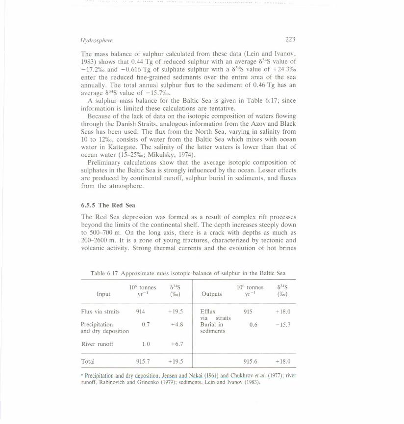
Hydrosphere 223

The mass balance of sulphur calculated from these data (Lein and Ivanov,1983) shows that 0.44 Tg of reduced sulphur with an average 334Svalue of-17.2%0 and -0.616 Tg of sulphate sulphur with a 334Svalue of +24.3%0enter the reduced fine-grained sediments over the entire area of the seaannually. The total annual sulphur flux to the sediment of 0.46 Tg has anaverage 334Svalue of -15.7%0.

A sulphur mass balance for the Baltic Sea is given in Table 6.17; sinceinformation is limited these calculations are tentative.

Because of the lack of data on the isotopic composition of waters flowingthrough the Danish Straits, analogous information from the Azov and BlackSeas has been used. The flux from the North Sea, varying in salinity from10 to 12%0,consists of water from the Baltic Sea which mixes with oceanwater in Kattegate. The salinity of the latter waters is lower than that ofocean water (15-25%0; Mikulsky, 1974).

Preliminary calculations show that the average isotopic composition ofsulphates in the Baltic Sea is strongly influenced by the ocean. Lesser effectsare produced by continental runoff, sulphur burial in sediments, and fluxesfrom the atmosphere.

6.5.5 The Red Sea

The Red Sea depression was formed as a result of complex rift processesbeyond the limits of the continental shelf. The depth increases steeply downto 500--700 m. On the long axis, there is a crack with depths as much as200--2600m. It is a zone of young fractures, characterized by tectonic andvolcanic activity. Strong thermal currents and the evolution of hot brines

" Precipitationanddry deposition,JensenandNakai(1961)andChukhrovetal. (1977);riverrunoff, Rabinovich and Grinenko (1979);sediments, Lein and Ivanov (1983).

Table 6.17 Approximate mass isotopic balance of sulphur in the Baltic Sea

106 tonnes 834S 106 tonnes 834SInput yr-1 (%0) Outputs yr-1 (%0)

Flux via straits 914 +19.5 Efflux 915 +18.0vIa straits

Precipitation 0.7 +4.8I

Burial in 0.6 -15.7and dry deposition sediments

River runoff 1.0 +6.7

Total 915.7 +19.5 915.6 +18.0

224 Stable Isotopes

have formed metal-bearing sediments. Sixteen underwater brine 'basins'have been discovered so far.

The salinity is substantially higher than that of the ocean due to intenseevaporation. It is 36.7%0in the southern and 40.5%0 in the northern partsof the sea. The salinity of thermal waters filling the depressions is muchhigher (up to 319%0in Atlantis II).

This unusual hydrothermal regime of the Red Sea is reflected in theisotopic composition of sulphur in the sediments (Hartman and Nielsen,1966; Kaplan et at., 1969).

The isotopic composition of sulphate from pore waters in metal-bearingsediments in the Atlantis depression is the same as those of brine andseawater sulphates. On this basis and other evidence, it is concluded thatbacterial sulphate reduction does not occur in these sediments (temperatureabout 60°C and salinity about 300%0). The sediments in this depressiondiffer from those normally found in the deep ocean. There are abnormallyhigh concentrations of sulphides, mainly sphalerite and to a lesser extentpyrite, whereas in normal sediments, pyrite prevails. In Atlantis II, there isalso gypsum, anhydrite, and elemental sulphur.

On the basis of 034S values, sulphur of the Red Sea may be separatedinto four groups: sulphates of pore waters in normal sediments (+ 23%0);sulphates of brines, sulphate minerals, and some pore waters (+ 15 to+ 23%0); sulphides, sulphate minerals, and elemental sulphur of metal-bearing sediments with temperatures higher than 50°C (+ 12 to + 15%0);and sulphides from normal sea sediments and depressions with brinetemperatures of less than 50°C (- 20 to - 37%0).

The sulphur isotope data demonstrate the existence of two sulphur cyclesin the Red Sea sediments. One is the normal type found in the water basinsand includes both abiogenic and biogenic reactions. The second is onlybiogenic and typical of thermal waters and highly mineralized sediments.Both systems and their interactions have not been adequately studied andit is impossible to calculate a mass isotopic balance. Sulphate in the bodyof the Red Sea is isotopically homogeneous and similar to that of oceanwater.

6.5.6 Conclusion

The isotopic composition of sulphur has been summarized for five inlandseas. With the exception of the Red Sea, they are distinguished by lowsalinities.

Many factors determine the isotopic composition of SOi- in continentalseas. The most important is water exchange with the World oceans, viastraits. The Azov, Baltic, and Caspian Seas are strongly influenced by riverrunoff bearing SOi- that is isotopically lighter than that of the ocean.

Hydrosphere 225

Sulphate in the Caspian Sea is also affected isotopically by efflux to Kara-Bogaz-Gol. An important factor for all the basins is bacterial sulphatereduction in bottom silt, resulting in the enrichment of heavy isotopes inSOi-.

The isotopic systematics of sulphur in sediments of continental seas issimilar to those of the ocean. The distinction is that the initial concentration

and isotopic composition of dissolved sulphate may be different.

6.6 RIVERS*

A comprehensive review of the isotopic composition of sulphur in rivers hasalready been published (Ivanov et al., 1983). This section therefore, willfocus primarily on more recent reports.

The ;)34S0i- in any river represents a mixture of the sulphur derivedfrom the soil, bedrock, and the atmosphere. It can be modified by bioticprocesses in the river and its watershed. In principle, the ;)34Smeasurementscan be used (a) to fingerprint the sources of sulphur and (b) as a naturaltag on the key pathways of sulphur transformation in riverine ecosystems.Combined measurements of the isotopic compositions of sulphur and oxygenin sulphate further constrains the possible sources, key processes, andpathways. So far, however, relatively little work has been done on sulphurisotope systematics in the watersheds of the major rivers of the world.

In an ambitious study, Longinelli and Edmond (1983) found fairly uniform1)34Svalues in the Amazon basin (Figure 6.15). The sulphur isotope datasuggest that a large fraction (over 60%) of the sulphate load of the riveroriginates from the Permian evaporites (1)34S,+ 10%0)in the Andes source.region. About 35% of the dissolved sulphate was attributed to oxidativeweathering of sulphides in bedrocks downstream in the drainage basin. Thecontribution of cyclic sulphate from rainfall was believed to be only 5%.The SOi- concentration in the Amazon River is only 3 mg £-1, which issimilar to the level one finds in many remote (unpolluted) headwater streamsdominated by atmospheric inputs. The conclusion that little of the sulphatein the Amazon is derived from the atmosphere is thus surprising consideringthe high frequency of volcanic activities in South America.

The ;)180 values of sulphate in the Amazon basin hover around +7.5%0upstream of the Tefe confluence (Figure 6.15). Below this point, a divergencedevelops with downstream 1)34Svalues becoming less than +3%0 in 1976,but increasing to +90/00in 1977. These values presumably reflect yearlydifferences in rates of SOi- uptake (assimilatory sulphate reduction) bythe local fauna and flora. The absence of discernable parallel effects in the

*J .R. Nriagu.

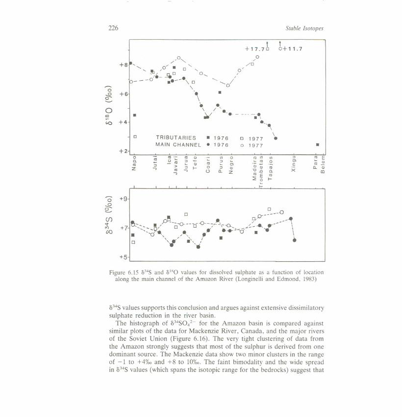
226 Stable Isotopes

t+17.70

°,/

/D

t0+ 1 1. 7

,°"",.. ,/ "-

+8,', 0/. 0 "-" ~ / 0 0""-8- ~ _e0- - - ° .e- \ 0"

0//

/

" "010

~0..........

+6" .

TRIBUTARIES. 1976MAIN CHANNEL. 1976

. e, --e\ / --e- - -- - . \

./ ._-,\e0 1977

a 1977 .

~0>c:

X

co E... <l>co -

a. <l>m

I

.--.0

~0..........

+9

(j)<tt<)ro

0

~ 0 0 0a- P r-. .f'<. 0- -.7'10-:- . / , r--~' / -- ...,.

+ -, -<:--cr 0 0 / -,-0., ..<-:: \. ''(J'''' . . .";-0' ... I" / /', - . \0 'I ."''fl . .

+5

Figure 6.15 8345 and 81HO values for dissolved sulphate as a function of locationalong the main channel of the Amazon River (Longinelli and Edmond, 1983)

334Svalues supports this conclusion and argues against extensive dissimilatorysulphate reduction in the river basin.

The histograph of 334S042- for the Amazon basin is compared againstsimilar plots of the data for Mackenzie River, Canada, and the major riversof the Soviet Union (Figure 6.16). The very tight clustering of data fromthe Amazon strongly suggests that most of the sulphur is derived from onedominant source. The Mackenzie data show two minor clusters in the rangeof -1 to +4%0 and +8 to 10%0.The faint bimodality and the wide spreadin 334Svalues (which spans the isotopic range for the bedrocks) suggest that

0 I.co.....

:t

"0

0C.a1Z

r/) 0 a1 r/) r/)a1'- co <l> ... ... ... co 0a1 -co ... CJ) -0;;

- ... <l>co> I- 0 <l>

u.Q C...., co ..., 0 a. z

co E co...,

::2' 0 I-...I-:-I I

Hydrosphere 227

Amazon '77

iAmazon '76

Q

~Mackenzie

I:] ",I:] 0 f1f:Ir:Jr:J~r.r.r.1 '"

USSR ...

.,...,.,,,,,

...,.,.".,.., """'...,.,.,.

-20 +32-10

Figure 6.16 834S0/- histographs for the Amazon, Mackenzie, and the major riversof the Soviet Union (data from Longinelli and Edmond, 1983; Hitchon and Krouse,

1972; Rabinovich and Grinenko, 1979)

the sulphur load in different segments of the river is controlled primarilyby inputs from small streams draining geological terrains with isotopicallydistinct signatures (see Hitchon and Krouse, 1972). The data for the Sovietrivers show a slightly skewed normal distribution about +6%0, although thedischarge weighted average was +8%0 (Rabinovich and Grinenko, 1979).The sulphur brought in by individual rivers, however, has distinctive isotopicimprints acquired from the bedrocks. The 034S0i- values of Soviet riversoften show pronounced seasonal changes which can result from (a) input ofgroundwater sulphate (the sole component during the base flow regime)and (b) the additional isotopically lighter sulphur from surface runoff.

Figure 6.17 shows the distribution of sulphur concentrations in the majorrivers of the world. The lowest mean SOi- concentration in a major riveris about 0.6 mg €-l in River Niger (Nriagu, 1986), whereas the arid Colorado

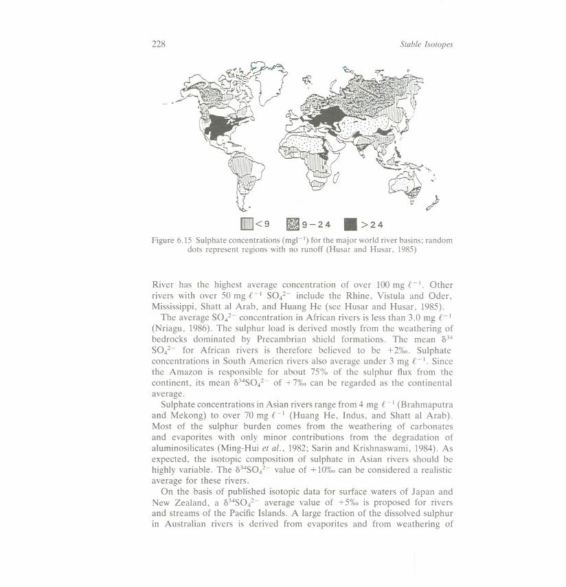
228 Stable Isotopes

.<9 119-24 .>24Figure 6.15 Sulphate concentrations (mgl-1) for the major world river basins; random

dots represent regions with no runoff (Husar and Husar, 1985)

River has the highest average concentration of over 100mg €- I. Otherrivers with over 50 mg €-l S042- include the Rhine, Vistula and Oder,Mississippi, Shatt al Arab, and Huang He (see Husar and Husar, 1985).

The average SOi- concentration in African rivers is less than 3.0 mg €-l(Nriagu, 1986). The sulphur load is derived mostly from the weathering ofbedrocks dominated by Precambrian shield formations. The mean 034SOi- for African rivers is therefore believed to be +2%0. Sulphateconcentrations in South Americn rivers also average under 3 mg €-I. Sincethe Amazon is responsible for about 75% of the sulphur flux from thecontinent, its mean 034S042- of +7%0 can be regarded as the continentalaverage.

Sulphateconcentrationsin Asianriversrange from 4 mg €-I (Brahmaputraand Mekong) to over 70 mg €-l (Huang He, Indus, and Shatt al Arab).Most of the sulphur burden comes from the weathering of carbonatesand evaporites with only minor contributions from the degradation ofaluminosilicates (Ming-Hui et al., 1982; Sarin and Krishnaswami, 1984). Asexpected, the isotopic composition of sulphate in Asian rivers should behighly variable. The 034S0i- value of + 10%0can be considered a realisticaverage for these rivers.

On the basis of published isotopic data for surface waters of Japan andNew Zealand, a 034S0i- average value of +5%0 is proposed for riversand streams of the Pacific Islands. A large fraction of the dissolved sulphurin Australian rivers is derived from evaporites and from weathering of

Hydrosphere 229

sulphide minerals in bedrocks. On the basis of the few published data, the034S0l- for Australian rivers can be assigned a provisional mean value of+ 12%0.

Sulphate concentrations in many rivers of Europe and central NorthAmerica now exceed 20 mg £-I, the average values for the two continentsbeing 28 and 26 mg £-1 respectively (Husar and Husar, 1985). Most of thesulphur burden is of anthropogenic origin, derived primarily from theburning of fossil fuels and smelting operations. On the basis of the availabledata in the literature, mean 034S0l- values for Europe and North Americahave been estimated to be +6 and +4%0 respectively.

From available data, a global average for 034S0l- in rivers is estimatedto be +7%0. This must be regarded as a very tentative value pending furtherstudies on the isotopic composition of sulphur in the major rivers of theworld.

6.7 GROUND WATER*

6.7.1. Introduction

The concentration and isotopic composition of aqueous sulphur compoundsin ground waters is determined by a variety of inputs and reactions (Figure6.18). In some areas, wet and/or dry fallout with subsequent evaporativeenrichment at ground surface is the dominant source. In other areas, anyor all of dissolution or precipitation of sulphate minerals, the oxidation ofpyrite or organic matter, bacterial reductions, and sulphide mineralizationmay be important. Thus, the use of environmental isotopes for the recognitionof anthropogenic sulphur in ground waters is a difficult task. Difficulties ininterpreting such data is one reason why, until recently, only a relativelysmall number of papers on the subject have been published. However,recent investigations clearly show that the 34Sand 180 contents of inorganic,aqueous sulphur compounds (primarily SOl-, HzS, or HS-) can provideinformation on

(a) the origin of sulphur;(b) biogeochemistry, evolution of ground waters; and(c) groundwater residence flow paths.

The geochemistry of many young and economically important groundwatersystems is controlled by the recharge environment, i.e. climatic conditions,precipitation and dry fallout, vegetation cover, soil and bedrock compositions,and depth to the water table. This environment determines how much and

'P. Fritz and R.J. Drimmie.

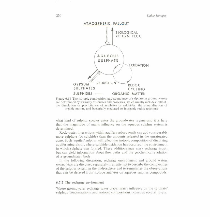
230 Stable Isotopes

ATMOSPHERICFALLOUT

!

BIOLOGICALRETURN FLUX

GYPSUMSULPHA TES

SULPHIDES -

REDOXCYCLING

ORGANIC MATTER

Figure 6.18 The isotopic composition and abundance of sulphate in ground watersare determined by a variety of sources and processes, which usually includes: fallout,the dissolution or precipitation of sulphates or sulphides, the mineralization of

organic matter, and bacterially mediated or inorganic redox reactions

what kind of sulphur species enter the groundwater regime and it is herethat the magnitude of man's influence on the aqueous sulphur system isdetermined.

Rock-water interactions within aquifers subsequently can add considerablymore sulphate (or sulphide) than the amounts released in the unsaturatedzone. Such 'aquifer' sulphur will reflect the isotopic composition of dissolvingaquifer minerals or, where sulphide oxidation has occurred, the environmentin which sulphate was formed. These additions may mask recharge input,but can yield information about flow paths and the geochemical evolutionof a groundwater body.

In the following discussion, recharge environment and ground waterssensu stricto are discussed separately in an attempt to describe the complexitiesof the sulphur system in the hydrosphere and to summarize the observationsthat can be derived from isotope analyses on aqueous sulphur compounds.

6.7.2 The recharge environment

Where groundwater recharge takes place, man's influence on the sulphate/sulphide concentrations and isotopic compositions occurs at several levels:

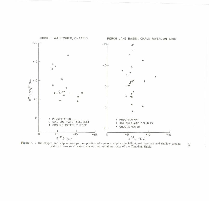
-t5 TIO TIS 0 ...S +10

8 34S (%0) 834S (%0)

Figure 6.19 The oxygen and sulphur isotopic composition of aqueous sulphate in fallout, soil leachate and shallow groundwaters in two small watersheds on the crystalline rocks of the Canadian Shield

0 +IS

NW......

DORSET WATERSHED, ONTARIO PERCH LAKE BASIN, CHALK RIVER, ONTARIO

T20r -tIOrtf

t:J.

I

t:J.

.TISf- l:> .,.St:J.I 0

l:> . .0 .

'8 TIO0

oL.

I 0 o.N", 00 0 t:J..

I

.(f) .0 0 0 . .0 0 0 --.ID .

""00-t5 o .I .

-S ..

oL l:> PRECIPITATION l:> PRECIPITATION0 SOIL SULPHATE (SOLUBLE) 0 SOIL SULPHATE(SOWBLE). GROUND WATER, RUNOFF . GROUND WATER

-10

232 Stable Isotopes

(a) Fallout in precipitation or as particulate matter, from reservoirs that arcapproximately equal in size (Kramer, 1975)

(b) Surface 'contamination' from waste disposal or fertilizer(c) Geochemical or biological reactions initiated through land cultivation,

irrigation, or drainage

Fallout and its isotopic composition has been described in Chapter 5. The0180 and 034Svalues of fallout are strongly dependent on the sulphur sourceand the meteorologic environment in which the oxidation to sulphateoccurred. Thus, in coastal environments, marine sulphate tends to dominate(0180 = +9.5%0 SMOW and 034S= +20%0). At inland stations, industrialor bacterial sulphur released from soils and open waters determines isotopiccompositions (Nriagu and Coker, 1978b). Terrestrial sources can be variablewith 0180 and 034S values as high as +20%0 (Holt et al., 1978; Krouse,1980). In general, anthropogenic sulphate has 034S values between 0 and+10%0 and 0180 values between +5 and +15%0.

In the upper soil zone, fallout participates in a number of biochemicalreactions. The nature of these is not yet fully understood, but the effectsof such transformations are clearly seen at two small watersheds in northernOntario, Canada.

Fallout in Ontario is strongly influenced by industrial emissions and typical0180 values vary between + 7 and + 15%0with extreme values as high as+ 25%0.The 034Svalues vary between 0 and + 10%0(Novicki, 1976; Holt etal., 1978; Feenstra, 1980). Shallow ground waters, however, show muchlower 0 values. This is shown in Figure 6.19 for the Perch Lake basin (ChalkRiver) and Plastic Lake watershed (Dorset).

Both basins are heavily forested. In the Perch Lake basin, the unsaturatedzone and the shallow aquifers overlying crystalline bedrock consist of up to20 m of uniform sand with simple mineralogies. No measurable amounts ofsulphate, sulphides, or carbonates are found in the unsaturated zone (2 mto water table). In the Plastic Lake basin, only a thin veneer of glacial tilloverlies the bedrock.

The 034Svalues of fallout in both watersheds are very similar and typicalfor industrial pollution in southwestern Ontario. Unfortunately, in bothstudies, the sampling periods were too short to record seasonal variationssimilar to those noted by Nriagu and Coker (1978a, 1978b). The 0180 valuesfor the fallout sulphate differ somewhat between the two basins, possiblybecause of differences in source and meteorological conditions.

Remarkably similar 034Svalues were found for sulphate in fallout, soilzone (water soluble), and shallow ground waters (Figure 6.20). This contrastssharply with the 0180 values in the different compartments, where significantdepletions in 180 between fallout and ground water/runoff are recognized.

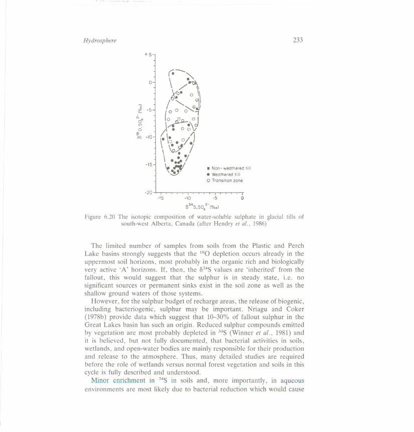
Hydrosphere 233

+5

-20-10 -5

8345,5042- (%.)

Figure 6.20 The isotopic composition of water-soluble sulphate in glacial tills ofsouth-west Alberta, Canada (after Hendry et af., 1986)

-15 0

The limited number of samples from soils from the Plastic and PerchLake basins strongly suggests that the 180 depletion occurs already in theuppermost soil horizons, most probably in the organic rich and biologicallyvery active 'A' horizons. If, then, the 034S values are 'inherited' from thefallout, this would suggest that the sulphur is in steady state, i.e. nosignificant sources or permanent sinks exist in the soil zone as well as theshallow ground waters of those systems.

However, for the sulphur budget of recharge areas, the release of biogenic,including bacteriogenic, sulphur may be important. Nriagu and Coker(1978b) provide data which suggest that 10-30% of fallout sulphur in theGreat Lakes basin has such an origin. Reduced sulphur compounds emittedby vegetation are most probably depleted in 34S (Winner et ai., 1981) andit is believed, but not fully documented, that bacterial activities in soils,wetlands, and open-water bodies are mainly responsible for their productionand release to the atmosphere. Thus, many detailed studies are requiredbefore the role of wetlands versus normal forest vegetation and soils in thiscycle is fully described and understood.

Minor enrichment in 34S in soils and, more importantly, in aqueousenvironments are most likely due to bacterial reduction which would cause

r.;--o \ /

O' °

I" °4

l -'] (0 0

o<t . OJ(06 . 0 \;

ro -10 \8\ 8 O/

\ J! 78 -;....-15-1. Non-weathered till

. Weathered till

0 Transition zone

234 Stable Isotopes

a preferential enrichment in 34Sand 180 in the residual sulphate (Mizutaniand Rafter, 1969). Uptake of sulphur by vegetation or bacterial activitiesand the mineralization of organic sulphur are expected to be important.This would involve reduction and oxidation reactions, which would cause a'readjustment' of the 0180 value of sulphate. The origin of oxygen in'secondary' sulphate depends on the environment in which oxidation takesplace. Under aerobic conditions, about two-thirds of the oxygen will comefrom the water and one-third from atmospheric oxygen (Lloyd, 1968; seeChapter 2), but in oxygen-poor environments, the 0180 value of the sulphatecan be very close to that of the water. In both cases, the observed depletionof 180 in soils and the unsaturated zone can be explained (Taylor et at.,1984; van Everdingen and Krouse, 1985).

Land cultivation, irrigation, and possibly fertilizers (Chesterikoff et at.,1981) contribute to salinization problems in many parts of the world, andas sulphate is often a major dissolved constituent in the saline waters,isotopic studies might reveal important information about its source. Forexample, on the prairies of southern Alberta, Canada, saline soils andground waters threaten large areas of agricultural land. Sulphate is a majorconstituent of these salts.

Canadian prairie soils in Alberta are largely developed on tills which sincedeglaciation have been subject to weathering to a depth of several metres.Organic carbon in the form of coal chips (Cret?.ceous) is abundant in manyareas. During weathering, this organic matter becomes oxidized and isbelieved to be the source of the sulphate. Isotope analyses on sulphatefound in shallow ground waters in recharge environments support thisinterpretation (Wallick, 1981; Wallick and Huemmert, 1983; Hendry et at.,1986). However, locally and in deeper strata, reduction does take place.Since bacterial or inorganic reduction will cause enrichments in both 180and 34S, a wide spectrum of isotopic compositions in the aqueous sulphateis found. The 034S values measured in this till aquifer vary between + 10and -30 permil%o (Shakur, 1982), with the more negative values beingattributed to the oxidation of reduced and isotopically depleted sulphur. Onthe other hand, where reduction is important, pyrite may precipitate a 034Svalue similar to this dissolved sulphide. Overall, this can result in a depthgradient with more positive 034S values in sulphur found at depth withinpartially reducing environments and lower 034Svalues near the top, whereoxidation of reduced sulphur becomes important.

Till deposits are typically very tight with very low hydraulic conductivities.Thus, it can take many weeks before piezometers yield enough water forchemical and isotopic analyses. Hendry et at. (1986) present, therefore,isotope data extracted directly from the tills of southern Alberta (Canada)by an aqueous extraction technique. Their findings (Figure 6.20) arestrikingly similar to the data shown in Figure 6.19. In both cases, the 034S

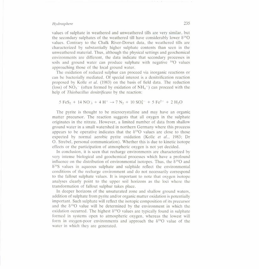
Hydrosphere 235

values of sulphate in weathered and unweathered tills are very similar, butthe secondary sulphates of the weathered till have considerably lower (')180values. Contrary to the Chalk River-Dorset data, the weathered tills arecharacterized by substantially higher sulphate contents than seen in theunweathered material. Thus, although the physical settings and geochemicalenvironments are different, the data indicate that secondary processes insoils and ground water can produce sulphate with negative 180 valuesapproaching those of the local ground water.

The oxidation of reduced sulphur can proceed via inorganic reactions orcan be bacterially mediated. Of special interest is a denitrification reactionproposed by Kolle et at. (1983) on the basis of field data. The reduction(loss) of N03 - (often formed by oxidation of NH4+) can proceed with thehelp of Thiobacillus denitrificans by the reaction:

5 FeS2 + 14 N03 + 4 H+ --3>7 N2 + 10 SO~- + 5 Fe2+ + 2 H2O

The pyrite is thought to be microcrystalline and may have an organi<:matter precursor. The reaction suggests that all oxygen in the sulphateoriginates in the nitrate. However, a limited number of data from shallowground water in a small watershed in northern Germany where this proceessappears to be operative indicates that the (')180values are close to thoseexpected by normal aerobic pyrite oxidation (Kolle et at., 1983; DrO. Strebel, personal communication). Whether this is due to kinetic isotopeeffects or the participation of atmospheric oxygen is not yet decided.

In conclusion, it is seen that recharge environments are characterized byvery intense biological and geochemical processes which have a profoundinfluence on the distribution of environmental isotopes. Thus, the (')180and(')34Svalues in aqueous sulphate and sulphide reflect the environmentalconditions of the recharge environment and do not necessarily correspondto the fallout sulphate values. It is important to note that oxygen isotopeanalyses clearly point to the upper soil horizons as the loci where thetransformation of fallout sulphur takes place.

In deeper horizons of the unsaturated zone and shallow ground waters,addition of sulphate from pyrite and/or organic matter oxidation is potentiallyimportant. Such sulphate will reflect the isotopic composition of its precursorand the (')180 value will be determined by the environment in which theoxidation occurred. The highest (')180values are typically found in sulphateformed in systems open to atmospheric oxygen, whereas the lowest willform in oxygen-poor environments and approach the (')180 value of thewater in which they are generated.

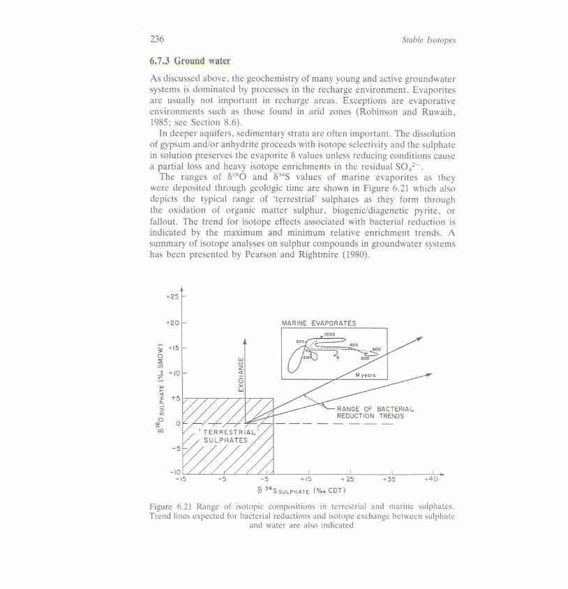
236 Stable Isotopes

6.7.3 Groundwater

As discussed above, the geochemistry of many young and active groundwatersystems is dominated by processes in the recharge environment. Evaporitesare usually not important in recharge areas. Exceptions are evaporativeenvironments such as those found in arid zones (Robinson and Ruwaih,1985; see Section 8.6).

In deeper aquifers, sedimentary strata are often important. The dissolutionof gypsum and/or anhydrite proceeds with isotope selectivity and the sulphatein solution preserves the evaporite 0 values unless reducing conditions causea partial loss and heavy isotope enrichments in the residual S042-.

The ranges of 0180 and 034S values of marine evaporites as theywere deposited through geologic time are shown in Figure 6.21 which alsodepicts the typical range of 'terrestrial' sulphates as they form throughthe oxidation of organic matter sulphur, biogenic/diagenetic pyrite, orfallout. The trend for isotope effects associated with bacterial reduction isindicated by the maximum and minimum relative enrichment trends. Asummary of isotope analyses on sulphur compounds in groundwater systemshas been presented by Pearson and Rightmire (1980).

+-25

+20 MARINE EVAPORATES

:s: +150~(J).~ +10

1000

wf-..J: + 5a...J::J(/)0

~co

RANGE OF BACTERIALREDUCTION TRENDS

-----

-5 + 15 + 25

/) 34S SULP",ATE(%. CDT)

Figure 6.21 Range of isotopic compositions in terrestrial and marine sulphates.Trend lines expected for bacterial reductions and isotope exchange between sulphate

and water are also indicated

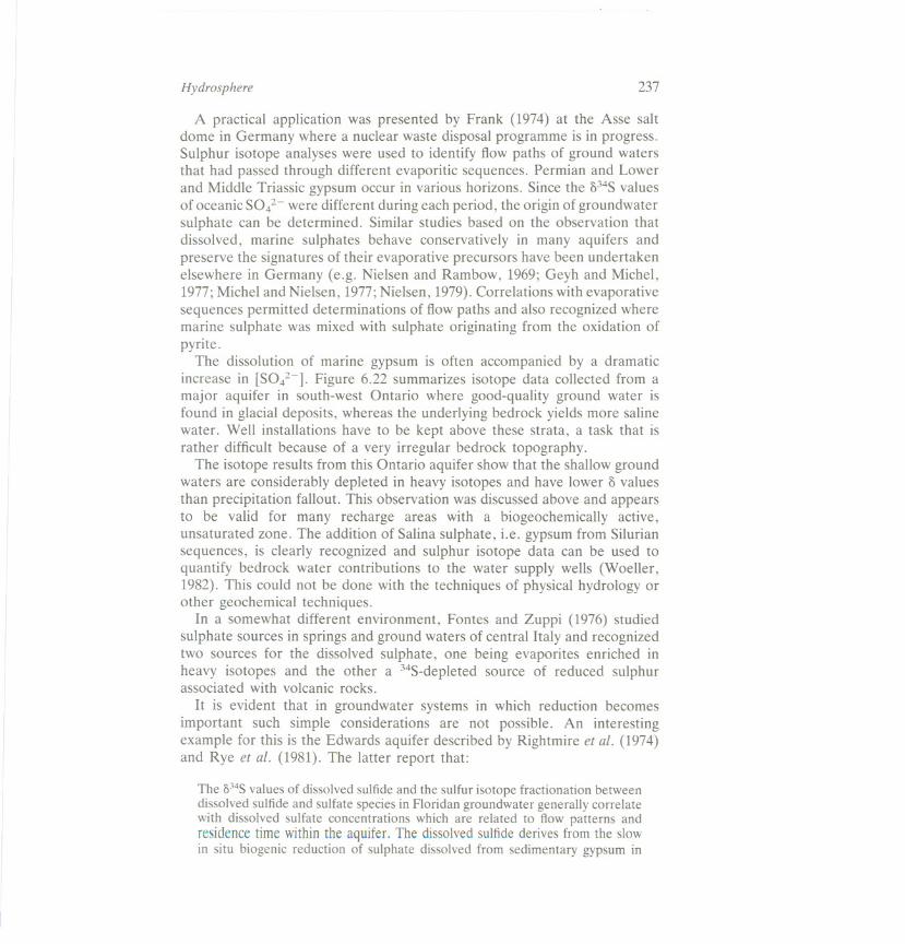
Hydrosphere 237

A practical application was presented by Frank (1974) at the Asse saltdome in Germany where a nuclear waste disposal programme is in progress.Sulphur isotope analyses were used to identify flow paths of ground watersthat had passed through different evaporitic sequences. Permian and Lowerand Middle Triassic gypsum occur in various horizons. Since the 334Svaluesof oceanic SOi- were different during each period, the origin of groundwatersulphate can be determined. Similar studies based on the observation thatdissolved, marine sulphates behave conservatively in many aquifers andpreserve the signatures of their evaporative precursors have been undertakenelsewhere in Germany (e.g. Nielsen and Rambow, 1969; Geyh and Michel,1977; Michel and Nielsen, 1977;Nielsen, 1979). Correlations with evaporativesequences permitted determinations of flow paths and also recognized wheremarine sulphate was mixed with sulphate originating from the oxidation ofpyrite.

The dissolution of marine gypsum is often accompanied by a dramaticincrease in [SOi-]. Figure 6.22 summarizes isotope data collected from amajor aquifer in south-west Ontario where good-quality ground water isfound in glacial deposits, whereas the underlying bedrock yields more salinewater. Well installations have to be kept above these strata, a task that israther difficult because of a very irregular bedrock topography.

The isotope results from this Ontario aquifer show that the shallow groundwaters are considerably depleted in heavy isotopes and have lower 3 valuesthan precipitation fallout. This observation was discussed above and appearsto be valid for many recharge areas with a biogeochemically active,unsaturated zone. The addition of Salina sulphate, i.e. gypsum from Siluriansequences, is clearly recognized and sulphur isotope data can be used toquantify bedrock water contributions to the water supply wells (Woeller,1982). This could not be done with the techniques of physical hydrology orother geochemical techniques.

In a somewhat different environment, Fontes and Zuppi (1976) studiedsulphate sources in springs and ground waters of central Italy and recognizedtwo sources for the dissolved sulphate, one being evaporites enriched inheavy isotopes and the other a 34S-depleted source of reduced sulphurassociated with volcanic rocks.

It is evident that in groundwater systems in which reduction becomesimportant such simple considerations are not possible. An interestingexample for this is the Edwards aquifer described by Rightmire et al. (1974)and Rye et al. (1981). The latter report that:

The 1)34Svalues of dissolved sulfide and the sulfur isotope fractionation betweendissolved sulfide and sulfate species in Floridan groundwater generally correlatewith dissolved sulfate concentrations which are related to flow patterns andresidencetime within the aquifer. The dissolved sulfide derives from the slowin situ biogenic reduction of sulphate dissolved from sedimentary gypsum in

238 Stable Isotopes

KITCHENER - WATERLOO AQUIFERS

illill+30 DEEP

{

GROUNDWATERIN CONTACTWITH SALINAGYPSUM

.

...

+20

0

~CL

!'"0'1:

U)"t 10vIf)

ro

..

.

SHALLOWGROUND

WATER

0'-

..

-10 0 + 1018 0

3 °SO 2-( YoO)4

Figure 6.22 The oxygen and sulphur isotopic composition of aqueous sulphate inthe Kitchener-Waterloo aquifers. References for the ranges of isotope values in thefallout areas: I-Holt et al. (1978), 2-Feenstra (1980), 3-Nriagu and Coker(1978a), and 4-Novicki (1976). Salina gypsum has a 034S= +28%0 (Miles, 1982)

+20

the aquifer. In areas where the water is oldest, the dissolved sulfidehas apparently attained isotopic equilibrium with the dissolved sulfate(034S= +65%0) at the temperature (28°C) of the system. This approach toequilibrium reflects an extremely slow reduction rate of the dissolved sulfateby bacteria; this slow rate probably results from very low concentrations oforganic matter in the aquifer.

I.

$ CD. .. 0

. 0- . @). . IIII

Hydrosphere 239

In the reducing part of the Edwards aquifer, Texas, there is a general down-gradient increase in both dissolved sulfide and sulfate concentrations, butneither the S34Svalues of sulfide nor the sulfide-sulfate isotope fractionationcorrelates with the groundwater flow pattern. The dissolved sulfide speciesappear to be derived primarily from biogenic reduction of sulfate ions whosesource is gypsum dissolution although up-gradient diffusion of HzS gas fromdeeper oil field brines may be important in places. The sulfur isotopefractionation for sulfide-sulfate (~38%0) is similar to that observed for modernoceanic sediments and probably reflects moderate sulfate reduction in thereducing part of the aquifer owing to the higher temperature and significantamount of organic matter present; contributions of isotopically heavy HzSfrom oil field brines are also possible.

A Cambro-Ordivician system in the North Central USA was studied byGilkeson et al. (1981). They present sulphur and oxygen isotope analyseson sulphate from an aquifer in which the recharge aqueous sulphate changesin 834S value from between 0 and + 7%0up to as high as + 30%0whereas8180 values increase from between 0 and +5%0to about + 17%0.Interesting,however, is the fact that 'ahead' of the reduced zone is an oxidized zone inwhich the dissolution of marine carbonates is recognized. The authorsexplain this somewhat unusual phenomenon as being due to recharge duringearlier, but still postglacial, times during which the reducing barrier had notyet been established. They also were able to document that excessively highbarium concentrations in these waters could be directly linked to sulphurgeochemistry.

It has been proposed that oxygen atoms in aqueous sulphate can exchangewith those of water (Figure 6.21). Lloyd (1968) presented experimental datawhich suggested half-times of between 104 and 105 years for this exchange.Thus, in very old groundwater sulphate, one might have expected a 8180value in equilibrium with that of the water. Recently, however, on the basisof extrapolation from elevated temperature experiments, Chiba and Sakai(1985) argued that the exchange is much slower with a half-time of theorder of 107 years.

A comparison of published oxygen isotope data for groundwater sulphatesand associated water strongly suggests that equilibration has not beensignificant. As indicated in Figure 6.21, it would cause an enrichment in180 only and none of the aquifers analysed shows such phenomena.

However, oxygen isotope exchange between sulphate and water apparentlyoccurs during sulphate reduction. As indicated above (Figure 6.21), bacterialreduction causes both 180 and 34Senrichments. As the product, i.e. reducedsulphur, is removed from the system, often as Fe-S minerals, both isotopesshould show Rayleigh behaviour. A 834Sversus 8180 plot should thus be astraight line, usually with a slope of 0.25-0.4. This, however, is notmaintained in all systems and both laboratory (Mizutani and Rafter, 1973;Fritz et al., in preparation) as well as field data (Basharmal, 1983; Fontes

240 Stable Isotopes

et at., 1985) strongly suggest that the initial Rayleigh behaviour of the tHOenrichments does change and asymptotically approaches a constant valuewhich is at least close to the expected value of the sulphate water equilibrium.This is shown in Figure 6.23.

The reaction sequence which permits such 'exchange' is not clear but ispossibly approximated by the following reaction paths:

S04Z-

H2OH

+ enzyme ~ SO/- enzyme complex ~ SO/- -3>HzSH

H2O

Overall SO/- ~ S032- equilibrationex:: 1.049

S032- ~ H2Oex::?

This shows the enzyme complexing of sulphate and its reduction to sulphiteand sulphide. Also indicated are possibilities for isotope exchange asproposed by Mizutani and Rafter (1973). This behaviour is shown in Figure6.24 which also summarized unpublished data by Fritz et al. (in preparation).

The laboratory data document that a 0180 difference between sulphatesand water of about + 30%0is approached if this difference is plotted againstthe residual sulphate of a reducing system. This is close, if not identical, tothe isotopic difference expected for isotopic equilibrium between water andsulphate.

The field data (Figure 6.24) come from a study in central Sweden andthe 'asymptotic' behaviour of OIHO,if compared to 034S, can be recognized.Again, the isotopic difference between sulphate and water is close to 30%0.

The isotope geochemistry of sulphur compounds in ground waters dependsstrongly on existing redox regimes. When oxidizing conditions prevail, theoxygen and sulphur isotopic compositions of sulphate in ground waters arediagnostic of the origin of the sulphate. It is usually possible to distinguishbetween sulphates added through the oxidation of reduced sulphur andcontributions from marine evaporites. The variable isotopic composition ofevaporites deposited during different geologic periods often permits ratherdetailed analyses of flow paths. Under favourable circumstances, isotopedata can be used in mass balance ca1culations that attempt to unravel mixingrelationships of different ground waters.

Bacterial reduction of sulphate causes both IHO and 34S enrichments.However, whereas the sulphur isotopic composition of the residual sulphateshows Rayleigh behaviour, the 0180 values approach those expected for

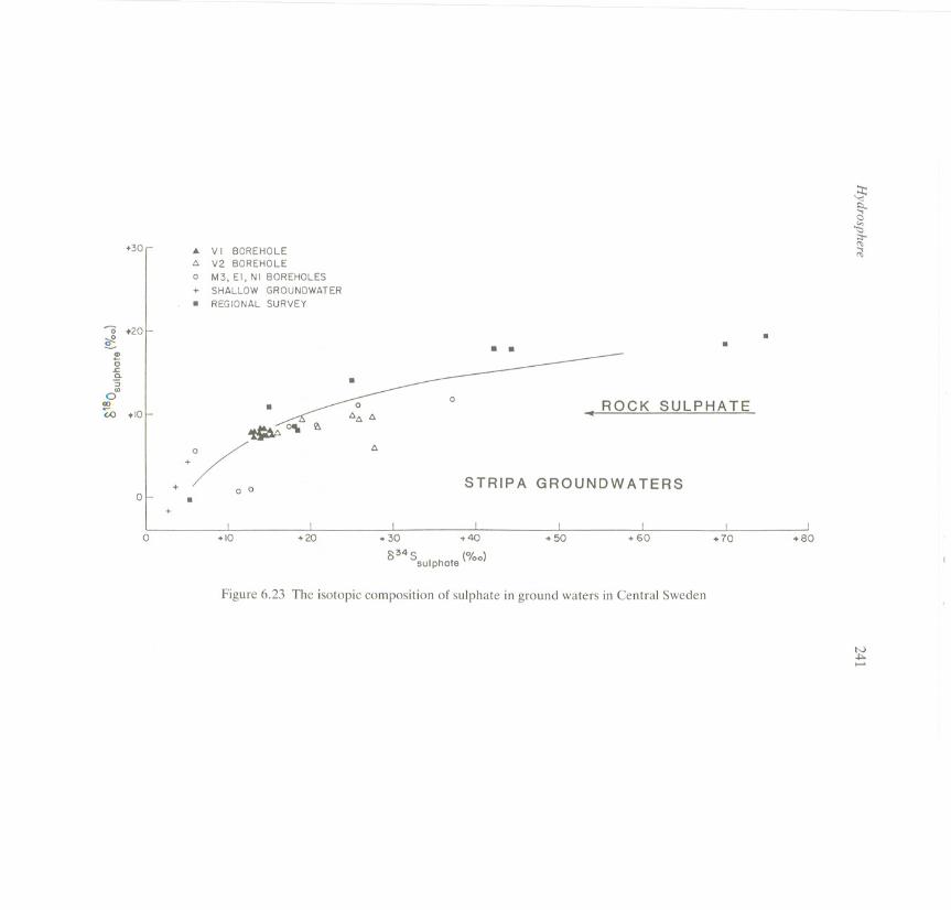
"0 ~20~~

.,0J:Q.:;en

0CD(.0 + 10

+30 . VI BOREHOLEl>. V2 BOREHOLE0 M3,EI,NI BOREHOLES+ SHALLOW GROUNDWATER. REGIONALSURVEY

0

. ..

. 0 0

~ OlIo~ l>.l>.l>.

../. --RQCK0 0

.

SULPHATE

STRIPA GROUNDWATERS.+0 +20 .30 +40

8345I h t (%0)

5U P a e

+10 + 50 + 60 .70

Figure 6.23 The isotopic composition of sulphate in ground waters in Central Sweden

.

.80

$~C1~~'"~

N.j::.......

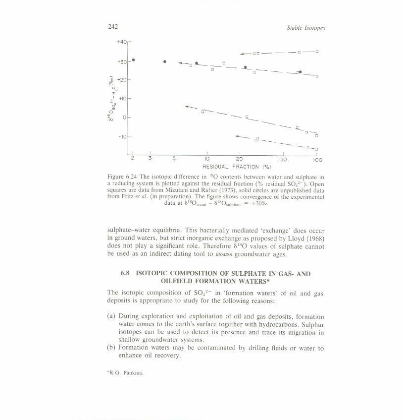
242 Stable Isotopes

+40

--00---0-0+30' 8 8

-0 - 0 - - - -~-o0 0

l +200 '":r:

!.,I +100"(f)

0

~ 0

12

13

-10

Figure 6.24 The isotopic difference in lXOcontents between water and sulphate ina reducing system is plotted against the residual fraction (% residual SO/-). Opensquares are data from Mizutani and Rafter (1973), solid circles are unpublished datafrom Fritz et al. (in preparation). The figure shows convergence of the experimental

data at ol~Owater - olXO,ulphatc = +30%0

sulphate-water equilibria. This bacterially mediated 'exchange' does occurin ground waters, but strict inorganic exchange as proposed by Lloyd (1968)does not playa significant role. Therefore 8180 values of sulphate cannotbe used as an indirect dating tool to assess groundwater ages.

6.8 ISOTOPIC COMPOSITION OF SULPHATE IN GAS- ANDOILFIELD FORMATION WATERS*

The isotopic composition of S042- in 'formation waters' of oil and gasdeposits is appropriate to study for the following reasons:

(a) During exploration and exploitation of oil and gas deposits, formationwater comes to the earth's surface together with hydrocarbons. Sulphurisotopes can be used to detect its presence and trace its migration inshallow groundwater systems.

(b) Formation waters may be contaminated by drilling fluids or water toenhance oil recovery.

*R.G. Pankina.

-------0-- ---- ----

------..Q........0-------- cP----

0--

-0-0I I I5 10 20 50 100

RESIDUAL FRACTION (%)

Hydrosphere 243

(c) Sulphate in formation waters can be biologically and thermochemicallyreduced to H2S. Oil and gas may be involved in the reduction process.

Thode et al. (1958) were the first to report on the isotope compositionof SOi- in formation waters of the Devonian Leduc field of Alberta,Canada (Table 6.18). The range in 834Svalues of 10%0can be explained byvariations in the isotope composition of Devonian evaporites (see Section4.3).

Data obtained by the author on the sulphur isotopic composition offormation water SO/- in gas- and oil-bearing strata of Devonian,Carboniferous, and Permian reservoir rocks in the Middle Volga region areshown in Figure 6.25. Waters in terrigenic deposits of the Middle and UpperDevonian are CaCh brines with very low [SO/-]. The gas does not containH2S and the 834S values of SO/- vary from +9.7 to + 16.8%0 over theregion. Since these values are lower than those of Devonian evaporites,there is a significant contribution of secondary sulphate.

The mineralization in waters in Lower Carboniferous deposits varies fromseveral milligrams to 280 g €-1. However, the Na+ ICl- coefficient is ratherstable (0.72-0.85). The [SO/-] content usually varies from 100 to2680 mg €-1. Most samples are enriched in 34Swhereas some approach theCarboniferous evaporite value (+ 14.0%0). The enrichments in 34S resultfrom intensive SO/- reduction, as shown by the presence of 34S-depletedH2S and the existence of sulphate reducing bacteria. Since the minimum834Svalues were only slightly lower than those for evaporites, contributionsfrom secondary sulphates leached from clays and sands prevailing in theregion are minor. In some cases, the lower 834S values might reflect anincursion of Lower Permian waters.

Waters from Middle Carboniferous deposits (mostly carbonate) are lessmineralized with higher S042- contents (up to 1560 mg €-l). However,there are regions where waters are more metamorphosed and contain lessSO/-. H2S is found in all dissolved gases. The isotopic composition of

Table 6.18 Isotope composition of SO/- of formation waters in Leduc deposit(0-2) (after Thode et al., 1958)

Well SOl-, ppm 834S, (%0)

314 743 +19.5527 541 +19.9308 550 +13.2271 676 +22.6153 625 +18.8Okalta Ireton 4 572 +12.6

244 Stable Isotopes

5~CE:NE:O

~5 I CRETACEOUS

en 5 I JURASSIC~ °

lL:c..:2 I« 10 I PERMIANen ILL I0 I

ffi°

LL:IX) I

5 10 : CARBONIFEROUSZ I

I

0

5~VONIAN0 0 +20

334S (%0)

Figure 6.25 Sulphur isotope composition of SO/- in formation waters of gas- andoilfields in the Middle Volga region. Vertical dashed lines are estimated mean 034S

for contemporaneous oceanic S042-

SOi- in these waters varies from +2.6 to + 19.7%0.The significant depletionsof 34S identify secondary sulphates as the dominant source. Even intensiveSOi- can result in insignificant 34Senrichment if the SOi- concentrationsare so high that the actual percentage of reduction is low.

In general, Permian waters are highly mineralized with concentrations ofSOi- up to 9400 mg £-1 and HzS up to 601 mg £-1. The isotopiccomposition of SOi- approximates that of Permian evaporites (+8.2 to+ 10.0%0).

Belyi and Vinogradov (1972) reported that SOi- in formation waters ofCretaceous and Jurassic deposits of the Amu-Daria syncline had 034Svaluesof +10.4 to +15.0%0 and +10.1 to +21.4%0 respectively.

Vredenburg and Cheney (1971) reported 034S values for SOi- information waters in the Wind River basin. In reservoir rocks of differentages, they found +9.1 to + 26.7%0for Mississippian, +9.5 to + 36.6%0 forPennsylvanian, + 14.5 to +23.4%0for Permian, + 12.4 to + 28.5%0for Triassic,+10.4 to +32.7%0 for Jurassic, and +6.4 to +14.3%0 for Cretaceous.

In the Big Horn basin, Orr (1974) reported 034Svalues for SO/- from+8.3 to +25.3%0 and +10.7 to +27.6%0 in formation waters contactingCarboniferous (Tensleep) and Permian (Phosphoria) deposits respectively.

The diversity of the isotopic composition of SO/- in formation waters isexplained by the combination of water-rock interactions and biological

Hydrosphere 245

activity. There may be a SOi- remnant from the original water in sediments.Additional SOi- may arise from the dissolution of evaporites (enriched in34S)or secondary sulphate minerals (often depleted in 34S). Surface or near-surface S04Z- transported downwards by meteoric water intrusion tends tohave lower 534Svalues than deeper evaporites.

6.9 GEOTHERMAL AREAS*

In volcanic and geothermal areas where fluids are derived from basic magmasat high temperatures, HzS is the dominant S-bearing gas and its isotopiccomposition reflects a magmatic source in the upper mantle. Typical 534Svalues are around 0%0:Kilauea +0.6 :t 0.2%0,Krafla (Iceland) +0.6 :t 0.3%0(Robinson, 1986), and Yellowstone 0 :t 3%0(Truesdell et at., 1978). Acidicmelts have higher SOzlHzS ratios, but as the temperature decreasesHzS becomes the dominant S-bearing gas in low-temperature fumaroles« 300°C) and geothermal systems. Its isotopic composition often stillreflects the magmatic source, but in this case there may have been aninvolvement of crustal rocks and crustal sulphur. The 534S values of netsulphur discharged from andesite volcanoes in Japan vary from +2.0 to+ 12%0as a consequence of crustal contamination (Sakai and Matsubaya,1977). Average 534S values for HzS in New Zealand geothermal systemsrange from +3.3 to +7.9%0, dominantly due to their setting in rhyolites/andesites (Robinson, 1986).

In the near-surface environment, the HzS oxidizes rapidly to [SOi-] insurface waters. Under the extreme conditions in volcanic crater lakes andfumaroles (S concentration 5-10 g kg-I; pH 1), such sulphate may have534S values up to + 20%0which can be interpreted as approaching isotopicequilibrium with the HzS (Robinson, 1978, in New Zealand; Sakai andMatsubaya, 1977, in Japan). Normally, however, the sulphate representscomplete or partial oxidation of HzS without any isotopic fractionation; e.g.Ketetahi hot springs in Mt Tongariro, New Zealand, have 534S values of+2.6 :t 0.7%0for sulphate which represents complete oxidation of HzS.

Sulphate is also present deep in geothermal systems but in much lowerconcentrations (30 mg kg-I at Wairakei, New Zealand). This primarysulphate has much higher 534S values (up to +24%0), representing anapproach to or attainment of isotopic equilibrium with HzS at temperaturesaround 350-370°C. Due to the slow rates of isotopic exchange, the high-temperature value is frozen in. If exchange rates are known, residence timesin the geothermal system can be calculated (Sakai, 1983). In contrast, oxygenisotopes in the sulphate exchange with water in the geothermal reservoirand can be used as a geothermometer (McKenzie and Truesdeli, 1977). The

'B.W. Robinson.

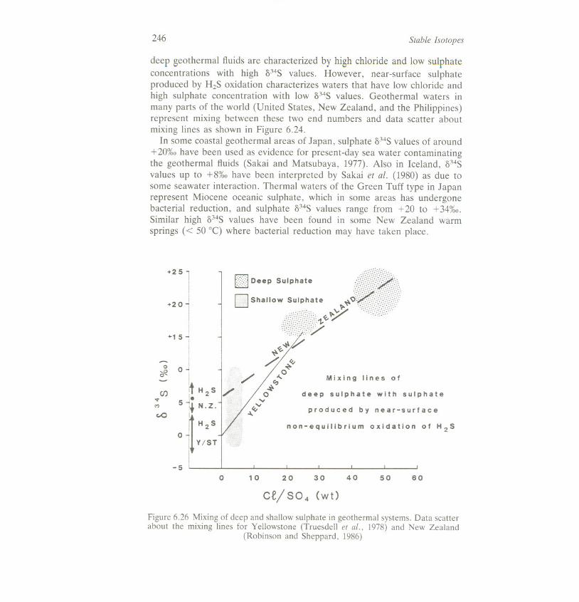
246 Stable Isotopes

deep geothermal fluids are characterized by high chloride and low sulphateconcentrations with high 034S values. However, near-surface sulphateproduced by H2S oxidation characterizes waters that have low chloride andhigh sulphate concentration with low 034S values. Geothermal waters inmany parts of the world (United States, New Zealand, and the Philippines)represent mixing between these two end numbers and data scatter aboutmixing lines as shown in Figure 6.24.

In some coastal geothermal areas of Japan, sulphate 034Svalues of around+20%0 have been used as evidence for present-day sea water contaminatingthe geothermal fluids (Sakai and Matsubaya, 1977). Also in Iceland, 034Svalues up to +8%0 have been interpreted by Sakai et al. (1980) as due tosome seawater interaction. Thermal waters of the Green Tuff type in Japanrepresent Miocene oceanic sulphate, which in some areas has undergonebacterial reduction, and sulphate 034S values range from + 20 to + 34%0.Similar high 034S values have been found in some New Zealand warmsprings « 50°C) where bacterial reduction may have taken place.

+25

+20

+15

CJ Deep Sulphate

..

l0

eft.

ii

i0-1

I

~ H2Si.

5l~

~

N.Z.

H2S0 '

l Y/STI

~~y

J:/~<v",0

~t:.:J0"

<v"~

Mixing lines of

if)'<tM

deep sulphate with sulphate

c..Oproduced by near-surface

non-equilibrium oxidation of H2S

-50 10 20 30 40 50 60

ct/S04 (Wt)

Figure 6.26 Mixing of deep and shallow sulphate in geothermal systems. Data scatterabout the mixing lines for Yellowstone (Truesdell et al., 1978) and New Zealand

(Robinson and Sheppard, 1986)

Hydrosphere 247

Continental geothermal areas in India have sulphate with a wide rangein 034S values: +6.5 to +37.5%0 (Giggenbach et al., 1983). The oxygenisotopic composition of this sulphate has equilibrated with the thermal waterdown to 100°C. Little alteration in the near-surface environment appearsto have taken place and the sulphate is thought to originate from sedimentarymaterial at depth.

6.10 WARM AND COLD SPRINGS*

6.10.1 Introduction

Sulphur isotope compositions have been measured for sulphur-containingcomponents in a number of springs throughout the world. To a lesser extent,0180 values for dissolved and related mineral sulphates have also beendetermined. The isotope data have proved useful in identifying strata withwhich these waters have interacted and elucidating associated physical,chemical, and biological processes.

Processes occurring in springs are site specific. Two subsurface sulphursource extremes can be considered: sulphide minerals and sedimentarysulphate (Muller et al., 1966; Pankina et al., 1966). It is highly likely thatthe dissolved S-containing ions are subsequently redistributed in responseto redox reactions and pH changes.

Sulphur isotope variations in thermal and cold springs of the world havebeen reviewed by Krouse (1974). For this volume, the sulphur isotopegeochemistry of a few springs where either sulphide or sulphate mineralswere primarily dissolved will be examined.

6.10.2 Springs containing primarily dissolved sulphate

In western Canada and probably world wide, the majority of dissolvedsulphur in warm and cold springs has origimted from the solution of sulphateminerals. In many cases, this sulphate is in evaporites deposited in ancientocean basins. Such springs often precipitate travertine.

The isotope geochemistry of these springs is essentially that of groundwater (Section 6.7) and its modification upon emergence. The concentrationof the dissolved ions are altered by pressure reduction, more aerobicconditions, and escape of gases to the atmosphere.

A dominant feature of these waters is that the dissolved sulphate oftenundergoes bacterial reduction and the sulphide product is markedly depletedin 34S. Data illustrating this isotopic selectivity for wells, boreholes, andsprings south of Great Slave Lake, Canada, are shown in Figure 6.27.

.H.R. Krouse.

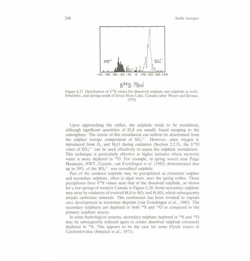
248 Stable Isotopes

HS-

8345 (0/00)Figure 6.27 Distribution of /)34Svalues for dissolved sulphate and sulphide in wells,boreholes, and springs south of Great Slave Lake, Canada (after Weyer and Krouse,

1979)

Upon approaching the orifice, the sulphide tends to be reoxidized,although significant quantities of H2S are usually found escaping to theatmosphere. The extent of this reoxidation can seldom be determined fromthe sulphur isotope composition of SOi-. However, since oxygen isintroduced from O2 and H2O during oxidation (Section 2.2.5), the &180value of SO i- can be used effectively to assess the sulphide reoxidation.This technique is particularly effective at higher latitudes where meteoricwater is more depleted in 180. For example, in spring waters near PaigeMountain, NWT, Canada, van Everdingen et at. (1982) demonstrated thatup to 30% of the SOi- was reoxidized sulphide.

Part of the oxidized sulphide may be precipitated as elemental sulphurand secondary sulphate, often in algal mats, near the spring orifice. Theseprecipitates have &34Svalues near that of the dissolved sulphide, as shownfor a few springs of western Canada in Figure 6.28. Some secondary sulphatemay arise by oxidation of evolved H2S to S02 and H2SO4which subsequentlyattacks carbonate minerals. This mechanism has been invoked to explaincave development in travertine deposits (van Everdingen et at., 1985). Thesecondary sulphates are depleted in both 34Sand 180 as compared to theprimary sulphate source.

In some hydrological systems, secondary sulphate depleted in 34Sand 180may be subsequently reduced again to render dissolved sulphide extremelydepleted in 34S. This appears to be the case for some Flysch waters inCzechoslovakia (Smejkal et at., 1971).

Hydrosphere 249

-30 -20 -10 0 +10 +20 +30834 S (%0)

Figure 6.28 Sulphur isotope variations in some selected springs from western Canada(after Krouse et al., 1970)

6.10.3 Springs containing primarily dissolved sulphide

In volcanic and geothermal areas, HzS is usually the dominant S-bearingspecies in the fluids and often has 034S values near 0%0, reflecting itsmagmatic source (see Section 6.9). There are, however, rare occurrences ofwarm and cold springs where dissolution of mineral sulphides constitutesthe main source of sulphur. Such springs often form colourful surfacedeposits of sulphate minerals such as jarosite. The ultimate origin of thesulphate from deeper mineral sulphide deposits is deduced from metal ioncontent, variable 034Svalues of the sulphate that are close to those of thedeep sulphide deposit, and 0180 values of the sulphate that may be highlynegative at high latitudes. A few such springs in western Canada werestudied by Shakur (1982).

Barite sinter deposits at Flybye Springs, NWT, Canada, were investigatedby Cecile et ai. (1984). Although the 034Svalues ranged from + 15 to +23%0,they were not as positive as barites in vugs of nearby Early to MiddleDevonian carbonate units (+29 to +32%0). Further, the 0180 values of thesinter barite were in the range -11 to -17%0, in contrast to the vug baritevalues of + 17 to + 26%0. The isotope data clearly show that the sinterdeposits did not result from simple dissolution of barite, transport, and

LOCATION oHS- .So- AALGAEoGYPSUM.S042-LASALINE

I I I I.MISSION .MIETTE ...COLD(JASPER)

UPPERl.L. KIDNEY .l.L.MIDDLEz CAVE .<X:BASINaJ

VERMILIONL. ...

HIGHWAYNO.1CANMORE .LUSSIERR. o .TURTLE MT.

I I I I

250 Stable Isotopes

precipitation. Rather, sulphate reduction occurred afterdissolution,andthesinter sulphate constitutes oxidized sulphide from that reduction.

6.10.4 Sulphur geochemistry of springs in relation to anthropogenicsulphur

From the viewpoint of this volume, the sulphur isotope geochemistry ofsprings is relevant to many aspects of anthropogenic sulphur in theenvironment. Emissions of gaseous sulphur compounds from certain springsare substantial, even to the point that high HzS concentrations threaten life.Emission rates have seldom been measured for individual springs and thecontributions to the atmospheric sulphur reservoir from springs world wideis not well known. There is the further complication that biogenic emissionsfrom some springs may vary with the seasons. Parameters that may changeseasonally include flow rate, temperature, pH, and EH. These in turninfluence the concentrations of S-containing ions and microbiologicalconversions. Consequently, the emissions may change in rate and isotopecomposition.

In local situations, seasonally dependent emissions from springs couldconceivably complicate assessments of anthropogenic contributions of Scompounds to the atmosphere. Conc~ntration measurements alone wouldprove inadequate. However, it is highly likely that the 334S values of thenatural and industrial emissions will differ sufficiently so that, in combinationwith concentration measurements, sources could be duly apportioned.

Another issue is the extent to which anthropogenic activities might alterthe S content and/or microbiological conversions in springs. It is noted thatanthropogenic perturbations need not be limited to the addition of sulphurcompounds. Introduction of other chemicals, such as nitrogen compoundsfrom fertilizer applications or organic nutrients, might upset physical chemicalparameters and microbial balances. Such effects are potentially more likelyin springs associated with shallow groundwater systems.

6.11 SUMMARY AND KEY AREAS FOR FURTHER RESEARCH*

The principal sulphur reservoirs in the ocean are shown in Figure 6.29. Withthe exception of the SOi- pool, reliable data on the sizes and isotopiccompositions of these reservoirs are currently not available. The transfer ofsulphur between the reservoirs involves physical, chemical, and biologicalprocesses, many of which are isotopically selective. Among the transform-ations, dissimilatory SOl- reduction has been recognized as being the mostdramatic in terms of S isotope fractionation, and typically results in

.J.O. Nriagu.

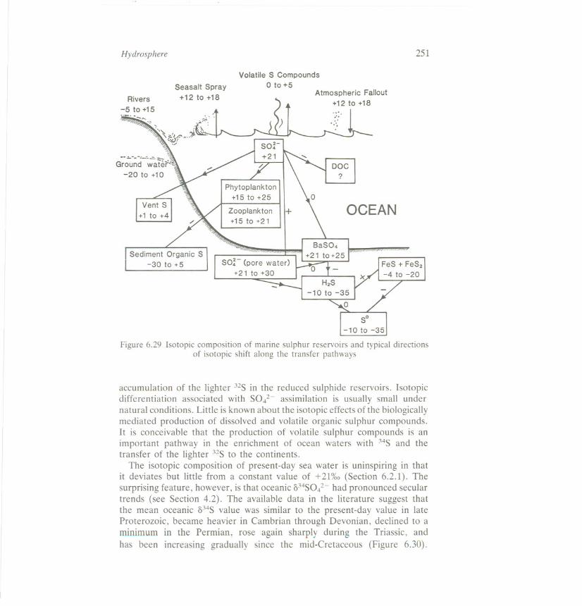
Hydrosphere 251

Seasalt Spray+12 to +18

Volatile S Compounds0 to +5

Figure 6.29 Isotopic composition of marine sulphur reservoirs and typical directionsof isotopic shift along the transfer pathways

accumulation of the lighter 32S in the reduced sulphide reservoirs. Isotopicdifferentiation associated with SOi- assimilation is usually small undernatural conditions. Little is known about the isotopic effects of the biologicallymediated production of dissolved and volatile organic sulphur compounds.It is conceivable that the production of volatile sulphur compounds is animportant pathway in the enrichment of ocean waters with 34S and thetransfer of the lighter 32S to the continents.

The isotopic composition of present-day sea water is uninspiring in thatit deviates but little from a constant value of +21%0 (Section 6.2.1). Thesurprising feature, however, is that oceanic 034S0i- had pronounced seculartrends (see Section 4.2). The available data in the literature suggest thatthe mean oceanic 034S value was similar to the present-day value in lateProterozoic, became heavier in Cambrian through Devonian, declined to aminimum in the Permian, rose again sharply during the Triassic, andhas been increasing gradually since the mid-Cretaceous (Figure 6.30).

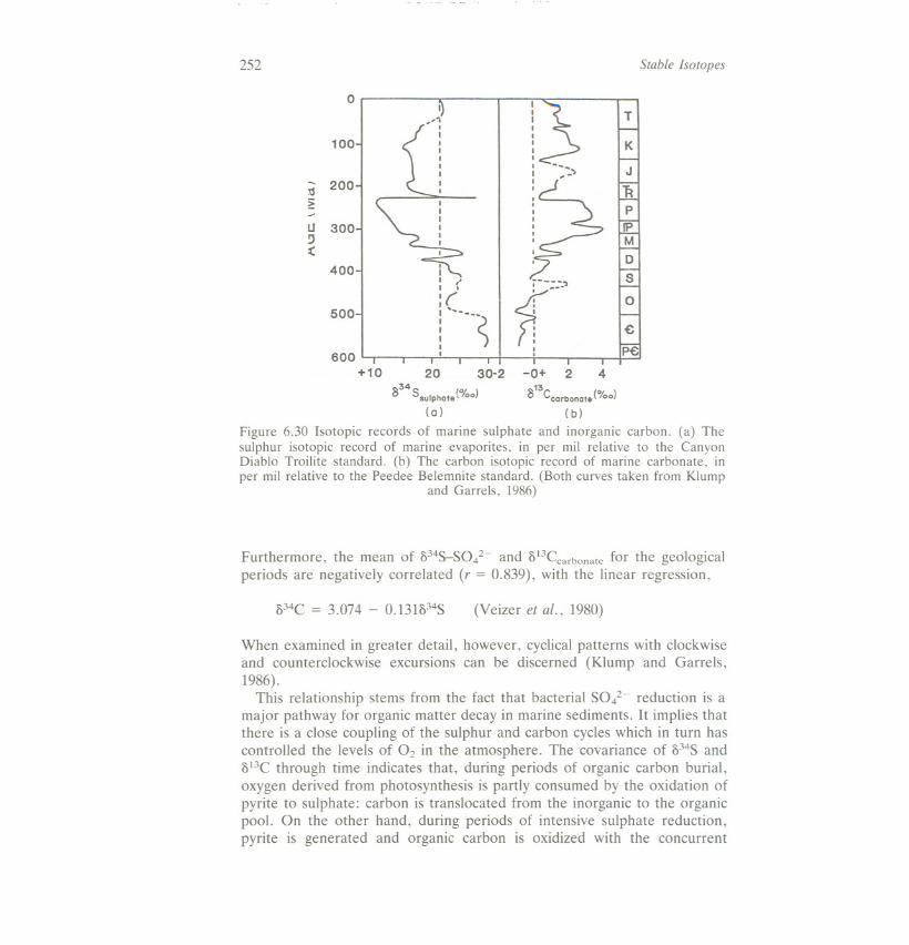
252 Stable Isotopes

0

100

I.."1'

I,IIIIIII

T

u!)~

300

K

J

RpIPMDS

0

~ 200~

400-1 I

~ /' ~;---~500-1 ! .~---s n, I

600 I I

+10 20 30-2 -0+ 2 4

8345 (°lc ) <>13sulpha,., 00 0 Ccarbana'. (0/00)

(0) (b)

Figure 6.30 Isotopic records of marine sulphate and inorganic carbon. (a) Thesulphur isotopic record of marine evaporites, in per mil relative to the CanyonDiablo Troilite standard. (b) The carbon isotopic record of marine carbonate, inper mil relative to the Peedee Belemnite standard. (Both curves taken from Klump

and Garrels, 1986)

~IP£

Furthermore, the mean of 034S-S0i- and o13Ccarbonatefor the geologicalperiods are negatively correlated (r = 0.839), with the linear regression,

034C = 3.074 - 0.131o34S (Veizer et al., 1980)

When examined in greater detail, however, cyclical patterns with clockwiseand counterclockwise excursions can be discerned (Klump and Garrels,1986).

This relationship stems from the fact that bacterial SOi- reduction is amajor pathway for organic matter decay in marine sediments. It implies thatthere is a close coupling of the sulphur and carbon cycles which in turn hascontrolled the levels of O2 in the atmosphere. The covariance of 034Sandol3C through time indicates that, during periods of organic carbon burial,oxygen derived from photosynthesis is partly consumed by the oxidation ofpyrite to sulphate: carbon is translocated from the inorganic to the organicpool. On the other hand, during periods of intensive sulphate reduction,pyrite is generated and organic carbon is oxidized with the concurrent

Hydrosphere 253

regeneration of the inorganic carbon pool. The linkage of the marinesulphur-carbon-oxygen cycles can be expressed by the following reactions:

8 SO~- + 2 Fez03 + 15 CHzO + 16 H+ ~ 4 FeSz + 15 COz + 23 HzO

or

2 Fez03 + SO~- + 16 COz + 8 HzO ~ 4 FeSz + 16 HC03 + 15 Oz

The SO~- includes seawater sulphate or evaporitic gypsum and anhydrite,and CHzO represents organic carbon.

The use of sulphur isotopes in deciphering the linkages between thesulphur cycle and the biogeochemical cycles of the other key elements (N,P, Si, Fe, 0, and C) remains a fruitful area for future research. In thisrespect, it should be noted that in a model in which the burial rate oforganic carbon increased by about 30%, the response of the oceanic o\3Cwas nearly instantaneous whereas the 034S value of SOl- changed at amuch slower rate, reflecting the long turnover time of the oceanic sulphatereservoir. Oxygen levels are predicted to respond fairly quickly in comparisonto the transfer of material between the oxidized and reduced reservoirs of

C and S. The latter approach their new steady-state masses and isotopiccompositions over several millions of years (Klump and Garrels, 1986).

The present-day biosphere shows a discern able dichotomy in the distri-bution of sulphur isotopes: 3ZStends to accumulate in terrestrial ecosystemswhereas the marine environment is enriched with the heavier 34S. The

available data are clearly inadequate to ascertain the implications of thisarrangement on the 034Sof the oceans (see Section 6.2.1). There is needfor isotopic measurements on the sulphur transported by the major riversof the world. Even less is known about the isotopic composition of thegroundwater sulphur reservoir (Section 6.7). Without these data, it will beimpossible to determine the overall isotopic balance which is necessary toevaluate published models of the global sulphur cycle.

Lakes and rivers constitute a tiny sulphur pool in comparison to oceans.Small inputs of sulphur from anthropogenic sources can thus significantlychange the concentrations and isotopic composition of the sulphur in manyfreshwater ecosystems. Indeed, lakes and rivers have become the criticaltarget ecosystems most susceptible to stress from acid rain (Section 6.4.1).

The reservoirs and principal transport pathways for sulphur in freshwaterecosystems are depicted in Figure 6.31. Since lacustrine environments aremostly sulphur deficient, the biota are less discriminating in their metabolismof sulphur isotopes and the fractionation by the various biogeochemicalprocesses generally tends to be small (compare Figure 6.29 and 6.31).

Sulphate reduction (equations above) has now been recognized as a majorsource of alkalinity in poorly buffered lakes (Kelly and Rudd, 1984; Carignan,

254 Stable Isotopes

Rivers-5 to +15

Volatile S Compounds0 to +5 Atmospheric Precipitation

0 to +15

-~"""--,.-:.~- "~.'...

Ground water'-5 to +5

",

1':::,:-

Figure 6.31 Typical a34s values of sulphur reservoirs of the lacustrine environments

1985). The sulphur cycle therefore plays an indirect key role in determiningthe response of a susceptible lake to acid rain inputs and the rate of recoveryof an acid-stressed lake. The reaction pathway for reduced sulphur infreshwater ecosystems differs from that of the marine cycle in onefundamental way: the HzS formed is tied up primarily by organic matterand, to a lesser extent, as 'FeS' (Nriagu and Soon, 1985; David and Mitchell,1985). Formation of pyrite, typical of marine environments, is very much aminor process and presumably occurs by a radically different pathwayinvolving the reaction of organic sulphur compounds with iron:

S-(L) + So + Fez+ ~ FeSz + U-S-(L) + HS- + FeH ~ FeSz + HL-

where (L) is any organic ligand. Evidence for the above reaction comesfrom the isotopic compositions of pyrite in lake sediments which are usuallyvery close to that of the organic sulphur fraction (Nriagu and Soon, 1985).Alternatively, organic Sand FeSz might arise from the same dissolvedsulphide. The actual process of organosulphur formation and the role ofthese compounds in the lacustrine sulphur cycle remains an important areafor research.

Hydrosphere 255

REFERENCES

Aizenshtat, Z., Stoler, A., Cohen, Y., and Nielsen, H. (1981). The geochemicalsulfur enrichment of recent organic matter of polysulfides in the Solar-Lake. In:Bjoroy, M., et al. (Eds.) Advances in Organic Geochemistry, Wiley, New York,pp. 279-88.

Almer, B., Dickson, W., Ekstrom, c., and Hornstrom, E. (1978). Sulfur pollutionand the aquatic ecosystem. In: Nriagu, J.O. (Ed.) Sulfur in the Environment,Vol. II, Wiley, New York, pp. 271-311.

Altschuler, Z.S., Schnepfe, M.M., Silber, c.c., and Simon, F.O. (1983). Sulfurdiagenesis in the Everglades peat and the origin of pyrite in coal. Science, 221,221-7.

Atkinson, L.P., and Hall, J.R. (1976). Methane distribution and production in aGeorgia salt-marsh. EST COAS M, 4 (6), 677-86.

Atlas of the Oceans (in Russian) (1977). Vols I and II, Leningrad, MO 555R, VMF.Ault, W.V., and Kulp, J.L. (1959). Isotope geochemistry of sulphur. Geochim.

Cosmochim. Acta, 16, 201-35.Banat, I.M., Lindstrom, E.B., NedwelL, D.B., and Balba, M.T. (1981). Evidence

for coexistence of two distinct functional groups of sulfate-reducing bacteria insalt marsh sediment. Appl. Environ. Microbiol., 42, 985-92.

Basharmal, M. (1983). The isotopic composition of sulphur compounds in landfills.M.Sc. thesis, University of Waterloo.

Beeton, A.M. (1965). Eutrophication of the St. Lawrence Great Lakes. Limnol.Oceanogr., 10, 240-54.

Belyi, V.M., and Vinogradov, V.I. (1972). Isotope composition of highly concentratedhydrogen sulfide gases in oil and gas bearing regions (in Russian). Geol. Nefti,Gaza, 7, 37-41.

Berner, R.A. (1971). Principles of Chemical Sedimentology, McGraw-Hill, NewYork.

Bouleque, J., Lord, c.J., and Church, T.M. (1982). Sulfur speciation and associatedtrace-metals (Fe-Cu) in the pore waters of Great Marsh, Delaware. Geochim.Cosmochim. Acta, 46 (3), 453-64.

Brunold, c., and Erisman, K.H. (1974). HzS as sulfur source for Lemna-minor Linfluence on growth; sulfur content and sulfate uptake. Experientia, 30 (5), 465-7.

Brunold, c., and Erisman, K.H. (1975). HzS as sulfate source in Lemna-minor L.2. Direct incorporation into cysteine and inhibition of sulfate assimilation.Experientia, 31 (5), 508-10.

Calvert, D.V., and Ford, H.W. (1973). Chemical properties of acid-sulfate soilsrecently reclaimed from Florida Marshland. Soil Sci. Soc., 37 (3), 367-71.

Carignan, R. (1985). Quantitative importance of alkalinity flux from the sedimentsof acid lakes. Nature, 317, 158-60.

Caron, F. (1984). Evaluation a l'aide des mesures des rapports des isotopes stablesdu soufre et de l'oxygine, de la proportion des sulfates mesures dans les lacsattributable aux depots atmospheriques. Thesis, Inst. National Recher. Scientif.Eau, University of Quebec, Quebec City.

Cecile, M.P., Goodfellow, W.D., Jones, L.D., Krouse, H.R., and Shakur, M.A.(1984). Origin of radioactive barite sinter, Flybye springs, Northwest Territories,Canada. Can. J. Earth Sci., 21 (4), 383-95.

Chambers, L.A. (1982). Sulfur isotope study of a modern intertidal environmentand interpretation of ancient sulfides. Geochim. Cosmochim. Acta, 46 (5), 721-8.

Chambers, L.A., and Trudinger, P.A. (1979). Microbiological fractionation of stablesulfur isotopes: a review and critique. Geomicrobiol. J., 1, 249-93.

256 Stable Isotopes

Chernovskaya,E,N" Pastukhova,N,M" Buinovich, A,G" ctal. (1965),Hydrochem-ical Regime of the Baltic Sea, Gidrometeoizdat, Leningrad, p. 168.

Chesterikoff, A., Lecolle, P., Letolle, R., and Carbonnel, J.P. (1981). Sulfur andoxygen isotopes as tracers of the origin of sulfate in Lake Creteil (southeast ofParis, France). J. Hydrol., 54, 141-50.

Chiba, H., and Sakai, H. (1985). Oxygen isotope exchange rate between dissolvedsulfate and water at hydrothermal temperature. Geochim. Cosmochim. Acta, 49,993-1000.

Chukhrov, F.V., Churikov, V.S., Yermilova, L.P., and Nosik, L.P. (1975). Variationsin the isotopic composition of sulphur in some natural water basins. Geokhimiya3, pp. 343-56; Geochem. Int., 12, 20-3l.

Chukhrov, F.V., Churikov, V.S., Yermilova, L.P., and Nosik, L.P. (1977). Isotopiccomposition of atmospheric sulphur and its possible evolution in the history ofthe Earth. Izvestiya Akad. Nauk SSSR,Ser. Geokh., 7, 4-13.

Claypool, G., Holser, W.T., Kaplan, I.R., Sakai, H., and Zak, I. (1980). The agecurves of sulfur and oxygen isotopes in marine sulfate and mutual interpretation.Chem. Geol., 28, 199-260.

Cook, R.B. (1981). The biogeochemistry of sulfur in two small lakes. Ph.D. Thesis,Columbia University, New York City, New York.

David, M.B., and Mitchell, M.J. (1985). Sulfur constituents and cycling in waters,seston, and sediments of an oligotrophic lake. Limnol. Oceanogr., 30, 1196-207.

Deevey, E.S. (1972). Biogeochemistry of lakes: major substances. In: Likens, G.E.(Ed.) Nutrients and Eutrophication, Vol. I, American Society Limnol. Oceanogr.,Special Symposia, pp. 14-19.

Deevey, E.S., Nakai, N., and Stuiver, M. (1963). Fractionation of sulfur and carbonisotopes in a meromictic lake. Science, 139, 407-8.

Dinur, D., Spiro, B. and Aizenshtat, Z. (1980). The distribution and isotopiccomposition of sulfur in organic-rich sedimentary rocks. Chem. Geol., 31, 37-5l.

Ellis, R.J. (1969). Sulfate activation in higher plants. Planta, 88 (1), 34-42.Eriksson, E. (1960). The yearly circulation of chloride and sulfur in nature;

meteorological, geochemical and pedological implications, part 2. Tellus, 12,63-109.

Faller, N. (1972). Sulfur dioxide, hydrogen sulfide, nitrous gases, and ammonia as solesources of sulfur and nitrogen for higher plants (in German). Z. Pfianzenernaehr.Bodenk., 131 (2), 130-8.

Feenstra, S. (1980). The isotopic evolution of sulphate in a shallow groundwaterflow system on the Canadian Shield. M.Sc. thesis, University of Waterloo,manuscript.

Fontes, J.C., and Zuppi, G.M. (1976). Isotopes and chemistry of sulphate bearingsprings of central Italy. In: Interpretation of Environmental Isotopes andGeochemical Data in Ground Water Hydrology, IAEA, Vienna, pp. 143-58.

Fontes, J.e., Michelot, J.L., and Fritz, P. (1985). Stable isotope geochemistry ofsulphur compounds. In: Stripa Project, Hydrogeological and HydrochemicalInvestigation in Boreholes, T.R., pp. 85-106, Ch. 7.

Frank, H. (1974). Hydrogeologische und hydrogeochemische Untersuchungen an derAsse bei Wolfenbuettel. Gesellsch. fuer Strahlenforsch., Bericht R-87 , Miinchen,p.208.

Friend, J.P. (1973). The global sulfur cycle. In: Rasool, S.I. (Ed.) Chemistry of theLower Atmosphere, Plenum Press, New York, pp. 177-20l.

Fritz, P., Fries, e.A., and Drimmie, R.J. (1986). Isotopic investigation of the sulfurcycle in selected Dorset watersheds. Final Report, Project No. 509-09. Departmentof Earth Sciences, University of Waterloo, Waterloo, Ontario, 32 pp.

Hydrosphere 257

Fritz, P., Drimmie, R.J., Ibsen, J., and Qureshi, R.M. (in preparation). Oxygenisotope equilibration during sulfate reduction.

Fry, B. (1986). Sources of carbon and sulfur nutrition for consumers in threemeromictic lakes of New York State. Limnol. Oceanogr., 31, 79-88.

Fry, B., Scalan, R.S., Winters, J.K., and Perker, P.L. (1982). Sulfur uptake by saltgrasses, mangroves, and seagrasses in anaerobic sediments. Geochim. Cosmochim.Acta, 46 (6), 1121-4.

Fry, B., Gest, H., and Hayes, J.M. (1983). Sulphur isotopic compositions of deep-sea hydrothermal vent animals. Nature, 306 (5), 51-2.

Garrels, R.M., and Thompson, M.E. (1962). A chemical model for seawater at25°C and one atmosphere total pressure. Am. 1. Sci., 260, 57-66.

Gershanovich, D.E., Gorshkova, T.I., and Konyukhov, A.I. (1974). Organicsubstance of modern suboceanic peripheral regions of continents. In: OrganicSubstance of Model and Fossil Sediments and Methods for Its Study (in Russian),Nauka, Moscow, pp. 63-80.

Geyh, M.A., and Michel, G. (1977). Zur Isotopenchemie von Mineralwassern undsonstigen Grundwassern im Heilquellengebiet von Bad Oeynhausen und BadSalzuflen. Fortschr. Geol. Rheinld. u. Westf., 26, 229-52.

Giggenbach, W.F., Gonfiantini, R., Jangi, B.L., and Truesdell, A.H. (1983). Isotopicand chemical composition of Parbati Valley geothermal discharges, North-WestHimalaya, India. Geothermics, 12, 199-222.

Gilkeson, R.H., Perry, E.C., and Cartwright, K. (1981). Isotopic and geologicstudies to identify the sources of sulfate in groundwater containing high bariumconcentrations. University of Illinois, Water Research Center Report 81-0165.

Goldhaber, M.B., and Kaplan, I.R. (1974). The sulfur cycle. In: Goldberg, E.D.(Ed.) The Sea, Vol. 5, Wiley, New York, pp. 569-655.

Gorham, E., Lund, J.W.G., Sanger, J.E., and Dean, W.E. (1974). Some relationshipsbetween algal standing crop, water chemistry and sediment chemistry in theEnglish lakes. Limnol. Oceanogr., 19, 601-17.

Gorlenko, V.M., Dubinina, G.A., and Kuznetsov, S.I. (1977). Ecology of aqueousmicroorganisms (in Russian), Nauka, Moscow, 288 pp.

Granat, L., Rodke, H., and Hallberg, R.D. (1976). The global sulphur cycle. In:Soderlund, R. (Ed.) Nitrogen, Phosphorous and Sulphur-Global Cycle, SCOPEReport 7, Ecol. Bull. (Stockholm), 22, 89-134.

Grinenko, V.A., and Grinenko, L.N. (1974). Geochemistry of Sulphur Isotopes,Nauka, Moscow, 272 pp.

Harrison, A.G., and Thode, H.G. (1958). Mechanism of bacterial reduction ofsulphate from isotope fractionation studies. Trans. Faraday Soc., 54, 84-92.

Hartman, M., and Nielsen, H. (1966). Sulfur isotopes in the hot brine and sedimentof Atlantis II deep (Red Sea). Marine Geol, 4, 4.

Hartman, M., and Nielsen, H. (1969). 34SWerte in rezenten Meeresedimenten undihre Deutung am Beispiel einiger Sedimentprofile aus der westlichen Ostsee.Geol. Rundschau, Bd., 58 (H3), 621-55.

Hendry, J., Cherry, J.A., and Wallick, E.I. (1986). Origin and distribution of sulfatein a fractured till in Southern Alberta, Canada. Water Resource Res., 22, 45-61.

Hitchon, B., and Krouse, H.R. (1972). Hydrogeochemistry of the surface waters ofthe Mackenzie River drainage basin, Canada: stable isotopes of oxygen, carbon,and sulfur. Geochim. Cosmochim. Acta, 36, 1337-57.

Holland, H.D. (1973). Systematics of the isotopic composition of sulfur in the oceansduring the Phanerozoic and its implications for atmospheric oxygen. Geochim.Cosmochim. Acta, 37, 2605-16.

258 Stable Isotopes

Holser, W.T., and Kaplan, I.R. (1966). Isotope geochemistry of sedimentary sulfates.Chem. Geol., 1, 93-135.

Holt, B.D., Cunningham, P.T., and Kumar, R. (1978). Seasonal variations ofoxygen-18 in atmospheric sulphates. Int. J. Environmental Analyt. Chem.(manuscript).

Horn, R.A. (1969). Marine Chemistry. The Structure of Water and Chemistry ofHydrosphere, Wiley-Interscience, New York, 568 pp.

Howarth, R.W., and Giblin, A. (1983). Sulfate reduction in the salt marshes atSapelo Island, Georgia. Limnol. Oceanogr., 28 (1), 70-82.

Howarth, R.W., and Teal, J.M. (1979). Sulfate reduction on a New England saltmarsh. Limnol. Oceanogr., 24 (6),999-1013.

Howarth, R.W., and Teal, J.M. (1980). Energy flows in a salt-marsh ecosystem: therole of reduced inorganic sulfur compounds. Am. Nat., 116 (6),862-72.

Howarth, R.W., Giblin, A., Gale, J., Peterson, B.J., and Luther, G.W. III (1983).Reduced sulfur compounds in the porewaters of a New England salt marsh.Environ. Biogeochem. Ecol. Bull. (Stockholm), 35 135-52.

Husar, R.B., and Husar, J.D. (1985). Regional river sulfur runoff. J. Geophys.Res., 90, 1115-25.

Ivanov, M.V. (1983). Major fluxes of the global biogeochemical cycle of sulphur.In: Ivanov, M.V., and Freney, J.R. (Eds.) The Global Biogeochemical SulphurCycle, SCOPE Report 19, Wiley, New York, pp. 449-63.

Ivanov, M.V., and Freney, J.R. (Eds.) (1983). The Global Biogeochemical SulphurCycle, SCOPE Report 19, Wiley, New York, 470 pp.

Ivanov, M.V., Lein, A. Yu., and Kashparova, E.V. (1976). Intensity of productionand diagenetic transformation of reduced sulphur compounds in the Pacific Oceansediments. In: Biogeochemistry of Diagenesis of Ocean Sediments (in Russian),Nauka, Moscow, pp. 171-8.

Ivanov, M.V., Grinenko, V.A., and Rabinovich, A.L. (1983). Sulphur flux fromcontinents to the ocean. In: Ivanov, M.V., and Freney, J.R. (Eds.) The GlobalBiogeochemical Sulphur Cycle, SCOPE Report 19, Wiley, New York, pp. 331-56.

Jannasch, H.W., Triiper, H.G., and Tuttle, J.H. (1974). Microbial sulfur cycle inthe Black Sea. In: Degens, E.T., and Ross, D. (Eds.) The Black Sea: its geology,chemistry and biology, American Association of Petroleum Geologists, No. 20.

Jeffries, M.a., and Krouse, H.R. (1984). Isotope Geochemistry of Stratified WaterBodies on Northern Ellesmere Island, Canadian Arctic, ZFI-Mitteilungen,pp. 159-69.

Jeffries, M.a., Krouse, H.R., Shakur, M.A., and Harris, S.A. (1984). Isotopicgeochemistry of stratified Lake 'A', Ellesmere Island, N.W.T., Canada. Can. 1.Earth Sci., 21, 1008-17.

Jensen, M.L., and Nakai, N. (1961). Sources and isotopic composition of atmosphericsulphur. Science, 134, 2102--4.

Jones, G.E., and Starkey, R.L. (1957). Some necessary conditions for fractionationof stable isotopes of sulfur by Desulfobibrio desulfuricans. Appl. Microbiol., 5,111-18.

Kaplan, LR., and Rittenberg, S.c. (1964). Microbiological fractionation of sulphurisotopes. J. Gen. Microbiol., 34, 195-210.

Kaplan, LR., Emery, K.O., and Rittenberg, S.c. (1963). The distribution andisotopic abundance of sulfur in recent marine sediments off Southern California.Geochim. Cosmochim. Acta, 27, 297-331.

Kaplan, LR., Sweeney, R., and Nissenbaum, A. (1969). Sulphur isotope studies onthe Red Sea geothermal brines and sediments. In: Degens, E.T. and Ross, D.A.

Hydrosphere 259

(Eds.) Hot Brines and Recent Heavy Metal Deposits in the Red Sea, pp. 263-71,Springer, New York.

Kelly, e.A., and Rudd, J.W.M. (1984). Epilimnetic sulfate reduction and itsrelationship to lake acidification. Biogeochem., 1, 63-77.

Kester, D.R., and Pytkowicz, R.M. (1969). Sodium, magnesium and calcium sulfateion-pair in seawater at 25°e. Limno!. Oceanogr., 14, 686-92.

King, G.M., and Wiebe, W.J. (1980). Regulation of sulfate concentrations andmethanogenesis in salt marsh soils. Estuarine Coastal Mar. Sci., 10 (2), 215-23.

Klump, L.R., and Garrels, R.M. (1986). Modeling atmospheric O2 in the globalsedimentary redox cycle. Am. J. Sci., 286, 337-60.

Kolle, W., Werner, P., Strebel, 0., and Bottcher, J. (1983). Denitrification byPyrite in a reducing aquifer. Vom Wasser, 61, 125-47.

Kramer, J.R. (1975). Atmospheric loading of the Upper Great Lakes. Acers ReportVol. 2, Canada Centre for Inland Waters, Burlington, Ontario.

Krouse, H.R. (1974). Sulphur isotope variations in thermal and mineral waters. In:Proceedings of International Symposium on Water-Rock Interaction (Int. Assoc.Geochem. Cosmochem.), Prague, Czechoslovakia, 9-19 September 1974 (Prague:Geological Survey 1976), pp. 340-7.

Krouse, H.R. (1980). Sulphur isotopes in our environment. In: Fritz, P., andFontes, J.e. (Eds.) Handbook of Environmental Isotope Geochemistry, Elsevier,Amsterdam, Ch. 11, pp. 435-71.

Krouse, H.R., and Ueda, A. (1987). Sulphur isotope analysis of trace sulphide andsulphate in various materials using Kiba reagents. In: Studies of Sulphur IsotopeVariations in Nature, International Atomic Energy Agency, Vienna, 1987. STIIPUBI747, ISBN 92--0-141087-5, pp. 113-21.

Krouse, H.R., Cook, ED., Sasaki, A., and Smejkal, V. (1970). Microbiologicalisotope fractionation in springs of Western Canada. In: Ogata, K., and Hayakawa,T. (Eds.) Recent Development in Mass Spectroscopy, Proceedings of InternationalConference on Mass Spectrometry, Kyoto, Japan, September 1969, UniversityPark Press, Chicago, pp. 629-39.

Krouse, H.R., Legge, A.H., and Brown, H.M. (1984). Sulfur gas emissions in theboreal forest: the West Whitecourt case study, V. Stable sulfur isotopes. Water,Air, Soil Pollut., 22, 321-47.

Lein, A. Yu. (1983). Biogeochemistry of anaerobic diagenesis of recent Baltic Seasediments. Eco!' Bull., 35, 441-61.

Lein, A. Yu., and Ivanov, M.V. (1983). Reduced sulphur accumulation sedimentsof marine basins with high rates of sulphate reduction. In: Ivanov, M.V., andFreney, J.R. (Eds.) The Global Biogeochemical Sulphur Cycle, Wiley, Toronto,pp. 413-20.

Lein, A. Yu., Namsaraev, RB., Trotsyuk, V. Ya., and Ivanov, M.V. (1981).Bacterial methanogenesis in Holocene sediments of the Baltic Sea. Geomicrobiol.J., 2 (4), 299-315.

Lein, A. Yu., Vainstein, M.B., Namsaraev, B.B., Kashparova, E.V., Matrasov,A.G., Bondar, V.A., and Ivanov, M.V. (1982). Biochemistry of anaerobicdiagenesis in recent sediments of the Baltic Sea. Geokhimiya, 3, 428-40.

Lein, A. Yu., Grinenko, V.A., and Migdisov, A.A. (1983). Isotope sulphur balancein oceanic sediments. In: Ivanov, M.V., and Freney, J.R. (Eds.) The GlobalBiogeochemical Sulphur Cycle, Wiley, New York, pp. 423-48.

Lew, M. (1981). The distribution of some major and trace elements in sedimentsof the Atlantic Ocean (DSDP samples). I. The distribution of sulfur, sulfurisotopes,and Mn, Fe, Zn, and Cu. Chern.Geol.,33(3-4), 205-24.

260 Stable Isotopes

Lloyd, R.M. (1968). Oxygen isotope behaviour in the sulfate-water system. J.Geophys. Res., 73, 6099-110.

Longinelli, A., and Edmond, J.M. (1983). Isotope geochemistry of the Amazonbasin: a reconnaissance. J. Geophys. Res., 88, 3703-17.

Luther, G.W. III, Giblin, A., Howarth, R.W., and Ryans, R.A. (1982). Pyrite andoxidation in salt marsh and estuarine sediments. Geochim. Cosmochim. Acta, 46,2665-9.

McKenzie, W.F., and Truesdell, A.H. (1977). Geothermal reservoir temperaturesestimated from the oxygen isotope compositions of dissolved sulfate and waterfrom hot springs and shallow drill holes. Geothermics, 5, 51-61.

MacLeod, D.A. (1973). Iron, manganese, and sulphur forms in salt marsh soils ofthe Wash, E. England and changes resulting from reclamation. In: Pseudogleyand Gley, Transactions of Commissions 5 and 6 of the International Society ofSoil Science, pp. 647-56.

Matrosov, A.G., Chebotarev, N. Ye, Kudryavtseva, A.J., Zyakun, A.M., andIvanov, M.V. (1975). Sulfur isotopic composition in freshwater lakes containingHzS. Geokhimiya 6, pp. 943-7; Geochem. Int., 12, 217-21.

Mekhtiyeva, V.L. (1971). Isotope composition of sulfur of plants and animals fromreservoirs of different salinity. Geokhimiya, 6, 725-30.

Mekhtiyeva, V.L. (1974). Application of sulphur isotope composition of fossil shellsto determine paleohydrochemical conditions in ancient water basins. Geokhimiya,11, 1682-7.

Mekhtiyeva, V.L. (1975). Isotope composition of sulphur of water soluble sulphateand living organisms from the Azov Sea. In: Chemico-oceanographic Studies ofSeas and Oceans, Nauka, Moscow, pp. 130-7.

Mekhtiyeva, V.L. (1980). Isotope composition of sulphur of sediments and brinesin ancient and recent Kara-Bogaz-Gol. Geokhimiya, 5, 745-53.

Mekhtiyeva, V.L., and Pankina, R.G. (1968). Isotope composition of sulphur ofwater plants and sulphates of water basins. Geokhimiya, 6, 739-42.

Mekhtiyeva, V.L., and Rabinovich, A.L. (1975). Isotope sulphur balance in theCaspian Sea. Okeanologiya, XV (1), 66-73.

Mekhtiyeva, V.L., Pankina, R.G., and Gavrilov, E. Ya. (1976). Distributionand isotope composition of sulfur in animal and plant tissues-hydrobionths.Geokhimiya, 9, 1419-26.

Michel, G., and Nielsen, H. (1977). Schwefel-Isotopenuntersuchungen an Sulphatenostwestfaelischer Mineralwasser. Fortschr. Geol. Rheinld. u. Westf., 26, 185-227.

Migdisov, A.A., Cherkosvsky, S.L., and Grinenko, V.A. (1974). Relation of theisotope composition of humid sediments and conditions of their formation.Geokhimiya, 10, 1482-502.

Migdisov, A.A., Ronov, A.B., and Grinenko, V.A. (1983). The sulphur cycle inthe lithosphere. Part I. Reservoirs in the global biogeochemical sulphur cycle.In: Ivanov, M.V. and Freney, J.F. (Eds.) The Global Biogeochemical SulphurCycle, SCOPE Report 19, Wiley, New York, pp. 25-94.

Mikulsky, Z. (1974). Water balance of the Baltic Sea. Vodnye Resursy, 5, 3-14.Miles, M. (1982). A study of the isotopic composition of the Salina Group gypsum

deposits at Caledonia (Ontario). B.Sc. thesis, University of Waterloo, 1982.Ming-hui, H., Stallard, R.F., and Edmond, J.M. (1982). Major ion chemistry of

some large Chinese rivers. Nature, 298, 550-3.Mitchell, M.J., Landers, D.H., and Brodowski, D.F. (1981). Sulfur constituents of

sediments and their relationship to lake acidification. Water, Air, Soil Pollut., 16,351-9.

Hydrosphere 261

Mitchell, M.J., David, M.B., and Uutala, A.J. (1984). Sulfur distribution in lakesediment profiles as an index of historical depositional patterns. Hydrobiology,121, No.2, 121-27.

Mizutani, Y., and Rafter, T.A. (1969). Oxygen isotopic composition of sulphates-part 4. N .2, J. Sci., 12, 60--8.

Mizutani, Y., and Rafter, T.A. (1973). Isotopic behaviour of sulphate oxygenisotopes in the bacterial reduction of sulphate. Geochem. J., 6, 183-91.

Monster, J. (1973). Lake Tanganyika: sulfur isotopic composition of a sedimentarycore and dissolved sulfate of lake water. Report 91, Department of Chemistry,McMaster University, Hamilton, Ontario.

Muller, G., Nielsen, H., and Ricke, W. (1966). Schwefel-Isotopen-Verhaltnisse inFormations-Wassern und Evaporiten Nord- und Siiddeutschlands (in German).Chern. Geol., 1, 211-220.

Nakai, N., and Jensen, M.L. (1967). Sources of atmospheric sulfur compounds.Geochern. J.., 1, 199-210.

Nakai, N., Wada, H., Kiyosu, Y., and Takimoto, M. (1975). Stable isotope studieson the origin and geological history of water and salts in the Lake Vanda area,Antarctica. Geochem. J., 9, 7-24.

Nedwell, D.E., and Abram, I.W. (1978). Bacterial reduction in relation and sulfurgeochemistry in two contrasting areas of saltmarsh sediments. Estuarine CoastalMar. Sci., 6, 341-51.

Nedwell, D.B., and Abram, I.W. (1979). Relative influence of temperature andelectron donor and electron acceptor concentration on bacterial sulfate reductionin salt marsh sediment. Microbiol. Ecol., 5 (1), 67-72.

Nedwell, D.B., and Banat, I.M. (1981). Hydrogen as an electron donor for sulfate-reducing bacteria in Hurries of salt marsh sediment. Microbio/. Eco/., 7, 305-13.

Nguyen, B.C., Gaudry, A., Bonsany, B., and Lambert, G. (1978). Reevaluation ofthe role of dimethyl sulfide in the sulfur budget. Nature, 275, 637-9.

Nielsen, H. (1965). Schwefelisotope im marinen Kreislauf und das 834Sder friiherenMeere. Geo/. Rundsch., 55, 160--72.

Nielsen, H. (1979). Sulfur isotopes. In: Jager, E., and Hunziker, J.C.S. (Eds.)Lectures in Isotope Geology (course), Springer-Verlag, Berlin, Heidelberg, NewYork, pp. 283-312.

Nielsen, H., and Rambow, D. (1969). S-Isotopenuntersuchungen an Sulphatenhessischer Mineralwasser. Notizbl. hess. L. Amt Bodenforsch., 97, 352-66.

Nissenbaum, A. (1978). Sulfur isotope distribution in sulfates from surface watersfrom the northern Jordan Valley, Israel. Environ. Sci. Tech., 12,962-5.

Nissenbaum, A., and Kaplan, I.R. (1972). Chemical and isotopic evidence for thein situ origin of marine humic substances. Limno/. Oceanogr., 17, 570--81.

Novicki, V. (1976). An investigation of the Kitchener aquifer system using the stableisotopes 180 and 34S. M.Sc. thesis, University of Waterloo.

Nriagu, J.O. (1973). Sulfur isotope abundance in the Great Lakes waters: apreliminary report. In: Proceedings of 16th Conference on Great Lakes Research,International Association of Great Lakes Research, Ann Arbor, Michigan,pp. 1038-43.

Nriagu, J.O. (1975). Sulfur isotopic variations in relation to sulfur pollution of LakeErie. In: Isotope Ratios as Pol/utant Source and Behavior Indicators, IAEA,Vienna, pp. 77-93.

Nriagu, J.O. (1984). Role of inland water sediments as sinks for anthropogenicsulfur. Sci. Total Environ., 38, 7-13.

Nriagu, lO. (1986). Chemistry of River Niger. I: Major ions. Sci. Total Environ.,58, 81-8. II: Trace metals. Sci. Total Environ., 58, 89-92.

262 Stable Isotopes

Nriagu, 1.0., and Coker, R.D. (1976). Emission of sulfur from Lake Ontariosediments. Limnol. Oceanogr., 21, 485-9.

Nriagu, 1.0., and Coker, R.D. (1978a). Isotopic composition of sulfur in atmosphericprecipitation around Sudbury, Ontario. Nature, 274, 883-5.

Nriagu, J. 0., and Coker, R.D. (1978b). Isotopic composition of sulfur in precipitationswithin the Great Lakes Basin. Tellus, 30, 365-75.

Nriagu, J.O., and Coker, R.D. (1983). Sulfur in sediments chronicles past changesin lake acidification. Nature, 303, 692--4.

Nriagu, J.O., and Harvey, H.H. (1978). Isotopic variation as an index of sulfurpollution in lakes around Sudbury, Ontario, Nature, 273, 223--4.

Nriagu, J.O., and Soon, Y.K. (1985). Distribution and isotopic composition of sulfurin lake sediments of northern Ontario. Geochim. Cosmochim. Acta, 49, 823-34.

Nriagu, J.O., Wong, H.K.T., and Coker, R.D. (1982). Deposition and chemistryof pollutant metals in lakes around the smelters at Sudbury, Ontario. Environ.Sci. Techno/., 16 (9), 551-60.

OME (1981). Studies of Lake and Watersheds near Sudbury, Ontario, OntarioMinistry of the Environment, Toronto, Ontario.

Off, W.L. (1974). Changes in sulfur content and isotopic ratios of sulfur duringpetroleum maturation-study of Big Horn basin Paleozoic oils. Bull. Am. Assoc.Pet. Geol., 50, 2295-318.

Ostroumov, E.A., and Volkov, 1.1. (1964). Sulfates in the bottom deposits of theBlack Sea. In: Proceedings of the Institute of Oceanology, USSR Academy.

Ostroumov, E.A., Volkov, 1.1., and Fomina, L.S. (1961). Distribution of sulphurcompounds in bottom sediments of the Black Sea. Proceedings of the Instituteof Oceanology, USSR Acad. Sci., 50, 93-129.

Pankina, R.G., and Mekhtiyeva, V.L. (1969). Isotopic composition of differentforms of sulfur in water and sediments of Sernoye Lake (Sergiyevsk mineralwaters). Geokhimiya 5, pp. 589-94; Geochem. Int., 6, 511-16.

Pankina, R.G., Mekhtiyeva, V.L. Grinenko, V.A., and Churmenteyeva, M.N.(1966). Sulphur isotope composition of sulphates and sulphides in sulphidic watersof various regions-caucausis in relation to their genesis (in Russian). Geokhimiya9, pp. 1087-94.

Pearson, J.F., and Rightmire, CT. (1980). Sulphur and oxygen isotopes in aqueoussulphur compounds. In: Fritz, P., and Fontes, J.C (Eds.) Handbook onEnvironmental Isotope Geochemistry, Elsevier, Amsterdam, Ch. 6, pp. 227-58.

Peterson, B.I., Steudler, P.A., Howart, R.W., Friedlander, A.I., Juers, D., andBowlers, F.P. (1983). Tidal export of reduced sulfur from salt marsh ecosystem.In: Hallberg, R. (Ed.) Environmental Biogeochemistry-Proceedings of 5thInternational Symposium (ISEB), 1981, Ecology Bulletin (Stockholm) 35,pp. 153-65.

Pringle, CM., White, D.S., Rice, CP., and Tuchman, M.L. (1981). Biologicaleffects of chloride and sulfate with special emphasis on the Laurentian Great Lakes.Publication 20, Great Lakes Research Division, University of Michigan, AnnArbor, Michigan.

Rabinovich, A.L. (1971). Isotopic composition of sulphate ions of some groundwaters and factors of its formation. Candidate thesis, Novocherkassk.

Rabinovich, A.L., and Grinenko, V.A. (1979). Sulfate sulfur isotope ratios forUSSR river water. Geokhimiya 3, pp. 441-54; Geochem. Int., 16, 68-79.

Rabinovich, A.L., and Veselovsky, N.W. (1974). Isotopic composition of sulphateions of some surface ground waters and factors of its formation. Candidate thesis,Novocherkassk.

Rees, CE. (1970). The sulphur isotope balance of the ocean: an improved model.

Hydrosphere 263

Earth Planet. Sci. Lett., 7, 366-70.Rees, CE. (1978). Sulphur isotope measurements using S02 and SFo. Geochim.

Cosmochim. Acta, 42, 383-9.Rees, CE., Jenkins, W.J., and Monster, J. (1978). The sulphur isotopic composition

of ocean water sulphate. Geochim. Cosmochim. Acta, 42, 377-81.Rightmire, CT., Pearson, J.F., Back, W., Rye, R.O., and Hanshaw, B.B. (1974).

Distribution of sulphur isotopes of sulfates in groundwaters from the principalartesian aquifer of Florida and the Edwards aquifer of Texas, USA. In: IsotopeTechniques in Groundwater Hydrology, Vol. 2, IAEA, Vienna, pp. 191-207.

Robinson, B.W. (1978). Sulphate water and H2S isotopic thermometry in the NewZealand geothermal systems. U.S. Geological Survey Open File Report 78-701,pp. 354-6.

Robinson, B.W. (1987). Studies on Sulphur Isotope Variations in Nature, IAEA.,Vienna, pp. 31-48.

Robinson, E., and Robbins, R.C (1970). Gaseous sulfur pollutants from urban andnatural sources. J. Air Pollut. Control. Assoc., 20, 233-5.

Robinson, B.W., and Ruwaih, 1. (1985). The stable isotopic composition of waterand sulfate from the Raudhatain and Umm Al Aish freshwater fields, Kuwait.Chemical Geology-Isotope Geoscience, 58, 129-36.

Robinson, B.W., and Sheppard, D.S. (1986). A chemical and isotopic study of theTokaanu-Waihi area, New Zealand. J. of Volcanology and Geothermal Res., 27,135-51.

Romankevich, E.A. (1977). Geochemistry of Organic Matter in the Ocean (inRussian), Nauka, Moscow, 256 pp.

Rye, R.O., Back, W., Hanshaw, B.B., Rightmire, CT., and Pearson, J.F. (1981).The origin and isotopic composition of dissolved sulfide in groundwater fromcarbonate aquifers in Florida and Texas. Geochim. Cosmochim. Acta, 45, 1941-50.

Sakai, H. (1983). Sulfur isotope exchange rate between sulfate and sulfide and itsapplications. Geothermics, 12, 111-17.

Sakai, H., and Matsubaya, O. (1977). Stable isotope studies of Japanese geothermalsystems. Geothermics, 5, 97-124.

Sakai, H., Gunnlaugsson, E., Tomasson, J., and Rouse, J.E. (1980). Sulfur isotopesystematics in Icelandic geothermal systems and influence of seawater circulationat Reykjanes. Geochim. Cosmochim. Acta, 44, 1223-31.

Sarin, M.M., and Krishnaswami, S. (1984). Major ion chemistry of theGanga-Brahmaputra river system, India. Nature, 312, 538-41.

Sasaki, A. (1972). Variations in sulphur isotopic composition of oceanic sulphate.24th IGC, 1972, Sec. 10, pp. 342-5.

Schidlowski, M., Junge, CE., and Pietrek, H. (1977). Sulfur isotope variations inmarine sulfate evaporites and the Phanerozoic oxygen budget. J. Geophys. Res.,82, 2556--{j5.

SCOPE 19 (1983). Ivanov, M.V., and Freney, J.R. (Eds.) The Global BiogeochemicalSulphur Cycle, Wiley, Chichester, 470 pp.

Scopintsev, B.A. (1975). Formation of the Recent Chemical Composition of the BlackSea Waters. Gidrometeoizdat, Leningrad, 336 pp.

Shakur, M.A. (1982). 334S and 3180 variations in terrestrial sulfates. Ph.D. thesis,University of Calgary.

Shink, D.R. (1979). Review of marine geochemistry. In: U.S. National CommitteeReport: 17th General Assembly, IUGG Review of Geophysical Space Physics,Vol. 17, No.7, pp. 1447-73.

Skyring, G.W., Oshrain, R.L., and Wiebe, W.J. (1979). Sulfate reduction rates inGeorgia marshland soils. Geomicrobiol. J., 1 (4), 389-400.

264 Stable Isotopes

Skyring, G.W., Chambers, L.A., and Bauld, J. (1983). Sulfate reduction in sedimentscolonized by cyano-bacteria, Spencer Gulf, South Australia. Australian J. ofMarine and Freshwater Res., 34, 359-74.

Smejkal, V., Michalicek, M., and Krouse, H.R. (1971). Sulphur isotope fractionationin some springs of the Carpathian Mountain System in Czechoslovakia. Cas.Mineral Geol., 16, 275-83.

Smith, R.L., and Klug, M.J. (1981). Reduction of sulfur compounds in the sedimentsof a eutrophic lake basin. Appl. Environ. Microbiol., 41, 1230--7.

Stround, D.W., and Paynter, M.J.B. (1980). Enumeration of methanogenic andsulfate-reducing populations in a salt-marsh. In: Abstract of Annual Meeting ofAmerican Society of Microbiology, Washington, D.C., p. 203.

Taylor, B.C., Wheeler, M.C., and Nordstrom, D.K. (1984). Isotope composition ofsulphate in acid mine drainage as measure of bacterial oxidation. Nature, 308,538-41.

Thode, H.G., and Dickman, M. (1983).> Sediment sulfur distribution and itsrelationship to lake acidification in four lakes north of Lake Superior. UnpublishedContractual Report, Canada Center for Inland Waters, Burlington, Ontario.

Thode, H.G., and Dickman, M. (1984). Sulfur isotope distribution patterns andtheir relationship to acid rain in selected lakes north of Lake Superior. ResearchReport, Department of Chemistry, McMaster University, Hamilton, Ontario.

Thode, H.G., and Monster, J. (1964). Distribution of sulfur isotopes in evaporitesand ancient oceans. In: Chemistry of the Earth's Crust (in Russian), Vol. 2,Nauka, Moscow, pp. 589-600.

Thode, H.G., and Monster, J. (1965). Sulfur isotope geochemistry of petroleum,evaporites and ancient seas. In: Fluids in Subsurface Environments-A Symposium,American Association of Petroleum Geology Memo, 4, pp. 367-78.

Thode, H.G., Monster, J., and Dunford, H.B. (1958). Sulphur isotope abundancesin petroleum and associated materials. Bull. Am. Assoc. Petrol. Geol., 42,2619--41.

Thode, H.G., Monster, J., and Dunford, H.B. (1961). Sulphur isotope geochemistry.Geochim. Cosmochim. Acta, 25, 159-74.

Thomas, M.D., Hendricks, R.H., Collier, T.R., and Hill, G.R. (1943). Theutilization of sulfate and S02 for the S nutrition of alfalfa. Plant Physiol., 18,345-71.

Truesdell, A.H., Rye, R.O., Whelan, J.F., and Thompson, J.M. (1978). Sulfatechemical and isotopic patterns in thermal waters of Yellowstone Park, Wyoming.U.S. Geological Survey Open File Report 78-701, pp. 435-6.

Tsurikova, A.G., and Shulgina, E.F. (1964). Hydrochemistry of the Azov Sea,Gidrometeoizdat, Leningrad, 258 pp.

Ueda, A., and Sakai, H. (1983). Simultaneous determinations of the concentrationand isotope ratio of sulfate- and sulfide-sulfur and carbonate-carbon in geologicalsamples. Geochem. J., 17, 185-296.

van Everdingen, R.O., and Krouse, H.R. (1985). Isotope composition of sulphatesgenerated by bacterial and abiological oxidation. Nature, 315, 395-6.

van Everdingen, R.O., Shakur, M.A., and Krouse, H.R. (1982). Isotope geochemistryof dissolved, precipitated airborne and fallout sulfur species associated withsprings near Paige Mountain, Norman Range, NWT. Can. J. Earth Sci., 19,1395--407.

van Everdingen, R.O., Shakur, M.A., and Krouse, H.R. (1985). Role of corrosionby H2SO4 fallout in cave development in a travertine deposit-evidence fromsulfur and oxygen isotopes. Chem. Geol., 49, 205-11.

Veiser, J., Holser, W.T., and Wilgus, C.K. (1980). Correlation of 13CI2Cand 34S/

Hydrosphere 265

32Ssecular variations. Geochim. Cosmochim. Acta, 44 579-87.Vinogradov, A.P. (1953). The Elemental Chemical Composition of Marine Organisms,

New Haven Sears Foundation for Marine Research, New York, 687 pp.Vinogradov, A.P., Grinenko, V.A., and Ustinov, V.I. (1962). Isotopic composition

of sulphur compounds in the Black Sea. Geokhimiya, 10, 851-73.Volkov, 1.1. (1961). Iron sulfides, their interdependence and transformations in the

Black Sea bottom sediments. Tr. Inst. Okeanol., Akad. Nauk SSSR, 50, 68-92.Volkov, 1.1., and Rozanov, A.G. (1983). The sulfur cycle in Oceans-part I.

Reservoirs and fluxes. In: Ivanov, M.V., and Freney, J.R. (Eds.) The GlobalBiogeochemical Sulphur Cycle, The Scope Report 19, Wiley, Chichester,pp. 357-423, 440-8.

Vredenburg, L.D., and Cheney, E.S. (1971). Sulfur and carbon isotopic investigationof petroleum, Wind River Basin, Wyoming. Bull. Am. Assoc. Pet. Geol., 55,1954-75.

Wallick, E.I. (1981). Chemical evolution of groundwater in a drainage basin ofHolocene age, East Central Alberta, Canada. J. Hydrol., 54, 245-83.

Wallick, E.I., and Huemmert, M.RR. (1983). Overburden weathering study-Battle River Site. First year status summary. In: Assessment of ReclamationPotential and Hydrologic Impact of Large-scale Surface Coal Mining in PlainsAreas of Alberta, ARC, Edmonton, March 1983.

Weyer, K.U., and Krouse, RR. (1979). Investigations of regional geohydrology ofsouth of Great Slave Lake, NWT, Canada, utilizing natural sulphur and hydrogenisotope variations. In: Isotope Hydrology, Vol. 1, Proceedings of InternationalSymposium on Isotope Hydrology, Neuherberg, West Germany, 19-23 June,1978, IAEA, Vienna, pp. 251-64.

Winner, W.E., Smith, c.L., Koch, G.W., Mooney, H.A., Bewley, J.D., andKrouse, RR. (1981). Rates of emission of H2S from plants and patterns of stablesulphur isotope fractionation. Nature, 289, 672-3.

Woeller, R.M. (1982). Greenbrook Well Field Management Study 1981-1982. M.Sc.thesis, University of Waterloo.

Wright, R.F., and Snekvik, E. (1978). Acid precipitation: chemistry and fishpopulations in 700 lakes in southernmost Norway. Verh. Int. Verein. Limnol.,20, 705-75.