Hydraulic Modeling of an Automatic Upstream Water Level Control Gate for Submerged Flow Conditions

Hydraulic Modeling of an Automatic Upstream Water Level

Control Gate for Submerged Flow Conditions

Gilles BELAUD∗, Xavier LITRICO†, Bertus DE GRAAFF ‡, Jean-Pierre BAUME§

May 31, 2007

Abstract

The article proposes a mathematical model of an automatic upstream water level controlgate designed to operate under free and submerged flow conditions, called the Vlugtergate. This automatic gate controls the upstream level close to a design level, using acounterweight to compensate for the hydraulic pressure on the gate. The proposed gatemodel is an extension of an existing model for free flow conditions (Begemann gate) tosubmerged conditions. Submergence effects are introduced both in the discharge law andthe equilibrium law. The mathematical model is validated on experimental data from twosmall-scale gates and on data from literature, in order to show the ability of the model tosimulate the behavior of gates of various dimensions.

Keywords: upstream control, gate, hydraulic model, analytical model, submerged flow, labo-ratory tests.

Introduction

Flap gates are used in many open-channel networks to control upstream water levels. Thearticle deals with a specific type of gate, initially described by Vlugter (1940), and more recentlymentioned by Brouwer (1987), Brants (1996), de Graaff (1998), Burt et al. (2001) and Litricoet al. (2005). Such gates are installed in several irrigation projects, located in developingcountries such as Nigeria and Indonesia. They are used as an affordable mechanical means tocontrol water distribution, generally in conjunction with orifices or baffle modules to deliver adesired discharge in the distributary channels. Begemann and Vlugter gates were installed intwo Nigerian irrigation schemes built in the 1970’s (Brouwer, 1987): the Kano River IrrigationProject (KRIP) and the Hadejia Valley Irrigation Project (HVIP). Four cross regulators ofthe HVIP North Main Canal are equipped with a series of Vlugter and Begemann gates, andthe water distribution in the secondary channels of KRIP is performed with similar gates inconjunction with baffle modules.The considered automatic gate, the Vlugter gate, consists of a weir equipped with a steel platerotating around a horizontal axis located above the upstream water level (see Fig. 1). When

∗Associate Professor, ENSAM, 2 place Viala, 34060 Montpellier, France, e-mail: [email protected]†Researcher Hydraulic Engineer, Cemagref, UMR G-EAU, B.P. 5095, 34196 Montpellier Cedex 5, France,

e-mail: [email protected]‡Researcher hydrology, HKV consultants, Botter 11-29, 8232 JN, Lelystad, The Netherlands, e-mail:

[email protected]§Researcher Hydraulic Engineer, Cemagref, e-mail: [email protected]

1

the gate is open, water flows under the plate but also on its sides. A counterweight on the topof the plate compensates for the hydraulic pressure exerted by the water. When the upstreamwater level increases, the pressure also increases and the corresponding moment tends to openthe gate. When the water level decreases, the pressure diminishes and the moment exertedby the counterweight tends to close the gate. The equilibrium is obtained when the closingmoment exerted by the weight of the gate compensates for the opening moment exerted by thehydraulic pressure. When properly designed, such a gate can maintain upstream levels withina small range around the design upstream level (see Vlugter (1940); Burt et al. (2001)). Litricoet al. (2005) proposed a model to compute the water level and the gate opening for this typeof gates functioning in free flow conditions (Begemann or flap gates), based on discharge andequilibrium relationships.However, submerged conditions may be encountered in flat canals, where cross structures mustbe designed with little head loss. This paper deals with a modified version of the Begemanngate called the Vlugter gate, which is equipped with a cylindrical float on the downstream sideof the gate to limit the downstream influence on the gate. The hydraulic modelling of suchgates is rather challenging, mainly due to the flow configuration which is changing with thegate opening: for high opening angles, the gate behaves as a weir, while for small openingangles, its behavior is close to an orifice.To derive a mathematical model, these gates were observed in the field during two missions inNigeria and two small-scale laboratory gates have been designed and used for experimental dataacquisition: a reduced scale experimental gate was built in the laboratory canal of ENSAM(Ecole Nationale Superieure Agronomique de Montpellier, France), and another one was builtin the laboratory canal of Delft University of Technology, which we will refer to as the Delftgate.The first model developed by de Graaff (1998) based on the momentum conservation principlewas not able to accurately reproduce the gate behaviour for high flows and for high submergenceratios. This paper proposes an extension of the model of Litrico et al. (2005) to the submergedconditions for Vlugter gates, introducing submergence effects both in the discharge law andthe equilibrium law.The article is structured as follows: we first describe the behavior of the gate, then we presentthe experimental setup. In the next section, we derive the model of the Vlugter gate, withfirst the discharge law, then the equilibrium law and finally the combination of both in orderto predict the upstream water level and gate opening at equilibrium.

System Description and Behavior

Gate Description

The gate designed by Vlugter consists of a flap gate equipped with a float on the downstreamside. The float is a portion of a cylinder centered around the pivot line (point O, see Fig. 1)so that the moment exerted by the downstream water body is null, since the lever arm of thedownstream pressure force is null.The design water level, denoted hd, is the maximum upstream level in closed position. It maybe easily adjusted thanks to the counterweight. The location of the center of gravity, G, isusually referred to by the angle Φ, which is the angle between the horizontal and the planedefined the pivot line and G (see Fig. 1). The angle Φ has a large influence on the deviationfrom the design water level. A larger Φ results in a more sensitive gate and the sensitivity may

2

be so large that the gate may become unstable for large values of Φ (de Graaff, 1998). Somegates are equipped with dampers to reduce possible oscillations.

Figure 1: Vlugter gate, closed position

This study is based on experiments conducted in Delft (de Graaff, 1998) and ENSAM hydrauliclaboratories with two different gates. Vlugter’s original data were used for the model validation(Vlugter, 1940). The characteristics of the gates are given in table 1. We denote in the following:L the gate height (see Fig. 1), Bw the weir width, Bg the gate width, Lw the weir length, p thelever arm (distance between the pivot and the plate) and M the total mass of the gate. Theweir upstream and downstream heights are denoted hwu and hwd respectively. Note that Bg isslightly greater than Bw: in closed position, the contact width between the gate and the weiris 1.5 cm on each edge for ENSAM gate and 2 cm for Delft gate.

Table 1: Gate dimensions, Delft and ENSAM small scale gates. The horizontal and verticalcoordinates are denoted X and Z (see Fig. 1)

Specifications Delft gate ENSAM gate Vlugter gate(original data)

Weir length Bw 0.40 m 0.38 m 6 mGate width Bg 0.44 m 0.40 m 6 mGate height L 0.47 m 0.45 m 1.5 mHorizontal lever arm p 0.11 m 0.045 m 0.6 mTotal mass M 41.5 kg 24.1 kg 6350 kgAngle Φ {35,45,55} deg {38,45,58} deg 45 degCenter of gravity position G XG=0.15m, ZG variable XG variable, ZG=0.14m XG=0.7 m

Experimental Setup

ENSAM Gate

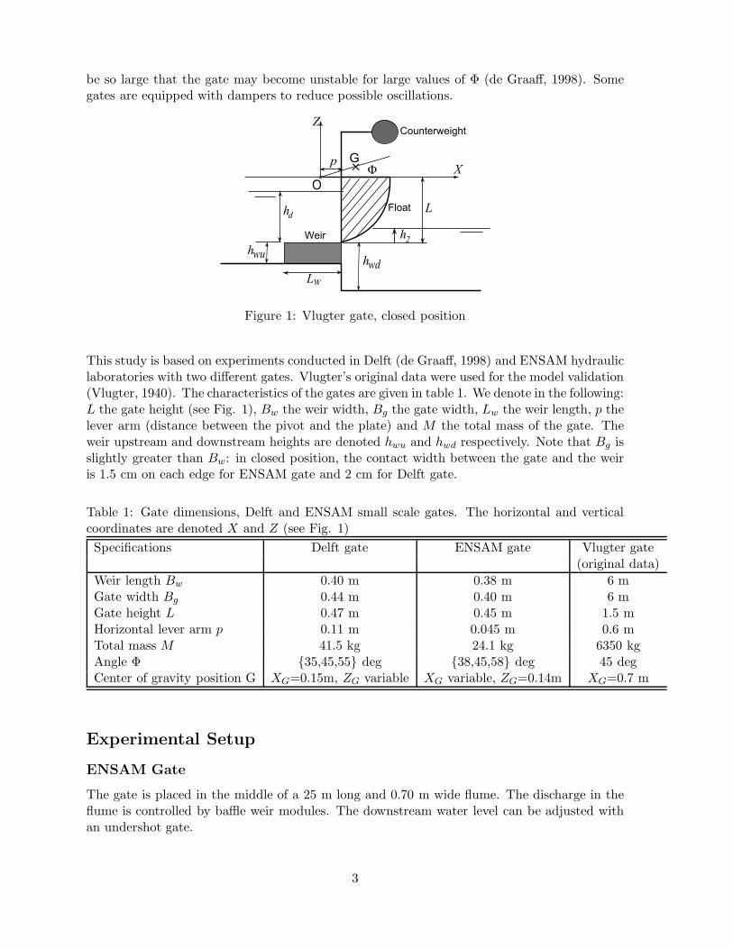
The gate is placed in the middle of a 25 m long and 0.70 m wide flume. The discharge in theflume is controlled by baffle weir modules. The downstream water level can be adjusted withan undershot gate.

3

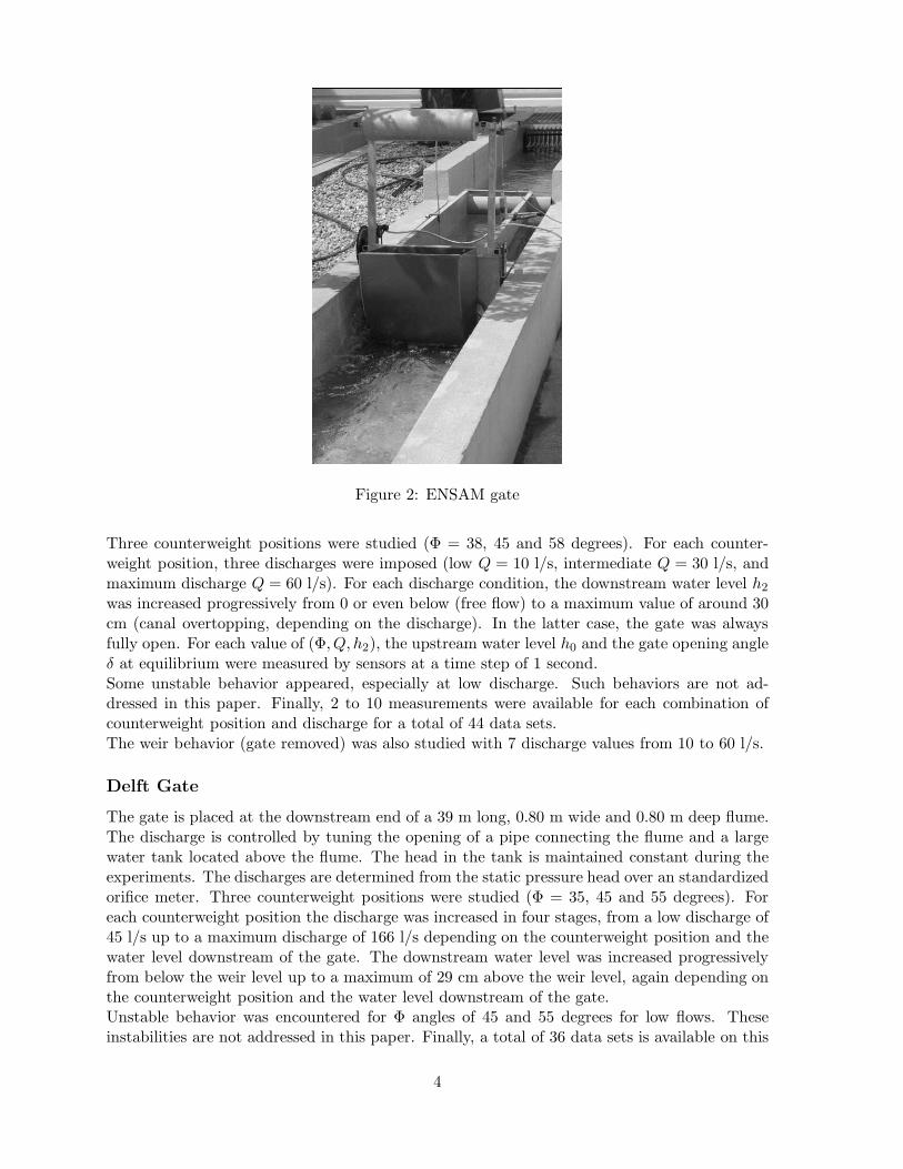
Figure 2: ENSAM gate

Three counterweight positions were studied (Φ = 38, 45 and 58 degrees). For each counter-weight position, three discharges were imposed (low Q = 10 l/s, intermediate Q = 30 l/s, andmaximum discharge Q = 60 l/s). For each discharge condition, the downstream water level h2

was increased progressively from 0 or even below (free flow) to a maximum value of around 30cm (canal overtopping, depending on the discharge). In the latter case, the gate was alwaysfully open. For each value of (Φ, Q, h2), the upstream water level h0 and the gate opening angleδ at equilibrium were measured by sensors at a time step of 1 second.Some unstable behavior appeared, especially at low discharge. Such behaviors are not ad-dressed in this paper. Finally, 2 to 10 measurements were available for each combination ofcounterweight position and discharge for a total of 44 data sets.The weir behavior (gate removed) was also studied with 7 discharge values from 10 to 60 l/s.

Delft Gate

The gate is placed at the downstream end of a 39 m long, 0.80 m wide and 0.80 m deep flume.The discharge is controlled by tuning the opening of a pipe connecting the flume and a largewater tank located above the flume. The head in the tank is maintained constant during theexperiments. The discharges are determined from the static pressure head over an standardizedorifice meter. Three counterweight positions were studied (Φ = 35, 45 and 55 degrees). Foreach counterweight position the discharge was increased in four stages, from a low discharge of45 l/s up to a maximum discharge of 166 l/s depending on the counterweight position and thewater level downstream of the gate. The downstream water level was increased progressivelyfrom below the weir level up to a maximum of 29 cm above the weir level, again depending onthe counterweight position and the water level downstream of the gate.Unstable behavior was encountered for Φ angles of 45 and 55 degrees for low flows. Theseinstabilities are not addressed in this paper. Finally, a total of 36 data sets is available on this

4

Figure 3: Delft gate

gate.The weir behavior was also studied with 7 discharge values from 45 to 170 l/s.

Mathematical Model of the Head-Opening-Discharge Relation-

ship

Basic principle

The model derived here calculates the discharge for given values of the upstream and down-stream levels (h0 and h2) and opening angle δ. The angle δ may differ from the equilibriumangle δ∗, by moving the gate manually for instance. Following the idea introduced in Litricoet al. (2005) for the Begemann gate, we consider that the gate behaves as an undershot gateat small openings, and as a broad-crested weir at large openings. Between these regimes, thevariation of the discharge Q with the opening angle is calculated by a cubic polynomial in-terpolation. The value of Q(δ) and its first order derivative is calculated in two characteristicpoints.

Calculation for Small Angles δ

When the gate is closed (δ = 0), the discharge equals 0 or a residual discharge Qr if any. Toanalyze the gate behavior, we also search for the derivative of Q with respect to δ. We firstconsider the free flow behavior, then we analyze the effect of submergence.

5

Calculation in free flow

Such as for Begemann gate (see Litrico et al. (2005)), the flow can be divided into two parts,one part flowing under the gate (Qu, area Au) behaving as a flow through an orifice, and onepart flowing on the sides (Qs), behaving as a flow over a weir. In the following, the subscriptf denotes for the free flow condition.

Figure 4: Vlugter gate, open position

Discharge under the gate, Quf – When δ increases, the discharge can be evaluated byapplying Bernoulli’s formula between the upstream reach and the contracted section below thegate. This yields the classical discharge formula (Bos (1989)):

Quf = CcAu

√

2g(H0 − h1) (1)

where Au is the opening area under the gate, Cc is the contraction coefficient, g the gravitationalacceleration, H0 the total upstream head and h1 is the hydrostatic head at the contractedsection. In free flow, the experiments showed that the value of h1 is small compared to H0.Eq. 1 is usually simplified as follows:

Quf = CuAu

√

2gh0 (2)

where Cu is a discharge coefficient, close to the contraction coefficient Cc and taking accountfor the approximation H0 − h1 ≃ h0.Au is calculated by multiplying the gate width, Bg, by the distance U between the bottom lipof the gate and the weir downstream edge. We obtain:

sin(δ/2) =U/2

L2 + p2(3)

and finallyAu = 2Bg

√

L2 + p2 sin(δ/2) (4)

From Eq. 2, we calculate the derivative of Quf in 0:

∂Quf

∂δ(0) = Cu

√

2gh0∂Au

∂δ(0) (5)

where∂Au

∂δ(0) = Bg

√

L2 + p2 (6)

6

Figure 5: Flow geometry, side discharge

Discharge on the sides, Qsf – The corresponding discharge Qsf is the one of a weir,the shape of which is illustrated on Fig. 5 (polygon ABCD). This discharge is obtained byintegrating the velocity,

√

2g(h0 − z), on the flow section (ABCD), where z is the height abovethe sill. The weir width, denoted b(z), is defined by:

z < Uv ⇒ b(z) = tan(δ/2)z (7)

z ≥ Uv ⇒ b(z) = Uh − tan(δ)(z − Uv) (8)

where Uv = L(1 − cos δ) + p sin δ is the vertical opening, and Uh = p(cos δ − 1) + L sin δ isthe horizontal opening (see Fig. 5). The flow is contracted, and it can be assumed that thecontraction coefficient is the same as for the flow under the gate, Cc, at least for small openings.We have

Qsf = 2Cc

∫ h0

0b(z)

√

2g(h0 − z)dz (9)

= 2√

2gCc

[

tan(δ

2)

∫ Uv

0z√

h0 − zdz +

∫ h0

Uv

(Uh − tan(δ)(z − Uv))√

h0 − zdz

]

(10)

which integrates in

Qsf = 2Cc√

2g[( 415h

5/20 − 2

5(h0 − Uv)3/2(2

3h0 + Uv)) tan( δ2 )

+23 (Uh + Uv tan(δ)) (h0 − Uv)

3/2 − 25 tan(δ)(h0 − Uv)

3/2(23h0 + Uv)]

(11)

The derivative in δ = 0 is obtained by expanding the above expression in Taylor series, whichyields

∂Qsf

∂δ(0) = 2

√

2gCc2

3h

3/20 (L − 2

5h0) (12)

Calculation in submerged conditions

In this case, h2 > 0. We first consider the discharge under the gate, Qu. Applying Bernoulli’sprinciple, equation 1 is still valid, but the head h1 is close to the downstream water level h2.Equation 1 writes as follows:

Qu = CuAu

√

2gh0(1 − s) (13)

where s = h2/h0 is the submergence ratio. In other terms, the discharge is multiplied by areduction factor due to submergence:

S(s) =√

1 − s (14)

7

and so it is for the derivative ∂Qu/∂δ(0).The same can be done for the side discharge, Qs. This discharge is obtained by multiplying theside discharge in free flow, Qsf , by a reduction factor S, such as usually done for submergedweirs (see (Sinniger and Hager, 1989; USDA, 1973; Hager and Schwalt, 1994; Bos, 1989) amongothers). In practice, it is difficult to estimate separately the flow under the gate from the flowon the sides and therefore to determine the modular limit and the reduction factor for the sideflow, which is not a usual weir. Different functions S(s) were tested for the side flow, but littledifference was observed between the different models. This is due to the fact that the dischargeunder the gate accounts for the major part of the total flow.Considering that the discharge relations for the flow under the gate and on the sides cannot becalibrated separately, we choose the same submergence function S(s) =

√1 − s and the same

contraction coefficient, Cc ≃ Cu, for both Qu and Qs. The combination of Eq. 5, 6, 14 and 12gives the derivative of Q in δ = 0:

∂Q

∂δ(0) = Cu

√

2gh0(1 − s)

[

Bg

√

L2 + p2 +2

3h0(2L − 4

5h0)

]

(15)

where Cu, discharge coefficient of the gate, should be around 0.6 to 0.9. The discharge coeffi-cients were obtained by calibration on the discharge curve data, leading to Cu = 0.85 for bothgates.

Weir Behavior

Weir formula

Here we analyze the flow when the gate is largely open. The gate has little influence on theflow, therefore we first consider the discharge through a weir, denoted Qw.For free flow, the classical formulation is used (Hager and Schwalt, 1994; Bos, 1989):

Qwf = CwBw

√

2gH3/20 (16)

in which Qwf denotes the discharge through the weir in free flow, H0 the total upstreamhead above the weir, Cw the weir discharge coefficient. This coefficient, close to 0.385, can beexpressed as a function of the weir length Lw, the upstream head H0, the weir upstream height(hwu) or downstream height (hwd). For a broad-crested weir, a simple formulation is adopted(Sinniger and Hager, 1989; Hager and Schwalt, 1994):

Cw = Cw0

(

1 − 2

9(1 + (H0/Lw)4)

)

(17)

in which Lw is the weir length and Cw0is a constant discharge coefficient.

As introduced before, submerged weirs can be modeled by using the free weir discharge equationand a reduction factor S = Qw/Qwf due to submergence. A classical formulation is used (see(Sinniger and Hager, 1989; Hager and Schwalt, 1994))

s1 = (s − yL) / (1 − yL) (18)

Sw = (1 − sm1

1 )m2 (19)

where yL is the modular limit of the weir (maximum value of s = h2/h0 for the free flowbehavior), m1 and m2 coefficients defined earlier. Such as suggested by Hager and Schwalt(1994) and Sinniger and Hager (1989), the values Cw0

= 0.435, yL = 0.75, m1 = 2 andm2 = 0.5 gave good results on the laboratory gates. Note that the weir behavior can be easilycalibrated by removing or opening manually the gate.

8

Figure 6: Influence of downstream level on δw

Calculation of δw

The discharge through the gate equals Qw as long as δ is greater than or equal to δw, angle forwhich the bottom lip of the gate touches the upper nappe of the flow. This angle is thereforeobtained by computing the intersection of the circle described by the bottom edge of the gateand the upper nappe profile. The computation of the upper nappe is then subject to threedifferent cases (see Fig. 6):

• When the downstream level is low (h2 < 0), the problem consists in determining theupper nappe profile generated by the free overfall (case 1).

• For higher downstream levels, but still in free flow, the circle described by the bottomedge of the gate may touch the free surface downstream from the jet issuing from thefree overfall. In this case, the contact point is between the jet and the hydraulic jumptransforming the kinetic energy of the jet into potential energy (case 2);

• When the weir is submerged (say, s = h2/h0 is above the modular limit yL), the uppernappe profile is modified (case 3).

Case 1: free flow, h2 ≤ 0: Such as for Begemann gate, the method proposed by Hager(1983) and Davis et al. (1999) was used to derive the equation of the upper nappe:

znappe = he − x tan α − x2 g

2V 2u cos2 α

(20)

with he brink depth (taken equal to 0.7 times the critical depth), Vu flow velocity through theweir, α angle of the flow with the horizontal at the brink, x the horizontal distance from thebrink and z the vertical abscissa taken from the sill. This angle is very small and is taken equalto 0◦, implying Vu = Q/(Bwhe).This profile is intersected with the trajectory of the bottom edge of the gate, which is a circle ofradius

√

L2 + p2 centered on the pivot line. The intersection calculation is made by a classicalzero-function search method and yields the value of δw. The coordinates of the intersectionpoint H (see Fig. 6) are denoted (xH , zH).

Case 2: free flow, yLh0 ≥ h2 > 0: The downstream influence is now considered. Since theflow through the weir is supercritical, a hydraulic jump occurs below the gate. The water level

9

below the gate can be roughly estimated by applying the momentum conservation principlebetween the brink (downstream end of the weir, section 1) and section 2 (downstream pool,see Fig. 6).The momentum of the jet, at the brink section, equals M1 = ρQVu = ρQ2/(Bwhe). In section2, it equals M2 = ρQ2/ (Bc(h2 + hwd)), where Bc is the canal width in the downstream pool.The forces exerted on the fluid are the pressure forces in section 1 and 2, Fp1 and Fp2. Insection 1, the water depth is h1 + hwd in the downstream pool and he in the jet issuing fromfrom the weir. The pressure force is given by

Fp1 =1

2ρgBc(h1 + hwd)

2 +1

2ρgBwh2

e (21)

Similarly, Fp2 = 12ρgBc(h2 + hwd)

2. The momentum principle writes as follows:

M1 + Fp1 = M2 + Fp2 (22)

and

1

2ρgBwh2

e +ρQ2/(Bwhe)+1

2ρgBc(h1 +hwd)

2 = ρQ2/ (Bc(h2 + hwd))+1

2ρgBc(h2 +hwd)

2 (23)

which gives

h1 =

√

√

√

√

(h2 + hwd)2 +Bw

Bch2

e −Q2

[

1Bwhe

− 1Bc(h2+hwd)

]

gBc− hwd (24)

At low discharge, both upstream and downstream momenta are low, and the same for he,calculated from the critical depth. From Eq. (24), it can be observed that h1 ≃ h2. Whenthe discharge increases, h2 being fixed, the momentum difference increases and the water levelbelow the gate decreases. This was indeed observed during experiments.Two situations may be observed:

• If h1 < zH , the angle δw is not affected by the downstream level and this case is equivalentto case 1;

• Otherwise the gate touches the water downstream from the nappe created by the overfall.We assume that the intersection appears upstream from the hydraulic jump, where thewater depth is h1. In this case, the intersection point J must verify:

zJ = h1 (25)

zJ = L(1 − cos(δw)) + p sin(δw) (26)

Introducing θ = tan(δw/2) and eliminating zJ , we get

δw = 2arctan(

√

p2 + L2 − (L − h1)2 − p

2L − h1) (27)

which is valid as long as 0 ≤ h1 < 2L. Let us remark that any level greater than L + p,which corresponds to δ = π/2, is unrealistic.

10

Case 3: submerged flow, yLh0 < h2: No hydraulic jump occurs. The water elevation ish2 in the downstream pool (except in the close vicinity of the brink). The intersection pointK must verify:

zK = h2 (28)

zK = L(1 − cos(δw)) + p sin(δw) (29)

which is solved the same way as for case 2:

δw = 2arctan(

√

p2 + L2 − (L − h2)2 − p

2L − h2) (30)

Derivative of Q with respect to δ

The only element missing for the cubic polynomial interpolation of the discharge formulas isthe variation of the discharge with δ. Observations showed that, such as for free flow, closingthe gate when δ ≈ δw does not affect the total discharge through the gate: the decrease of theflow rate below the gate is mainly compensated by the increase of discharge on the sides. Weassume that

∂Q

∂δ(δw) = 0 (31)

Full Discharge Equation

Given h0 and h2, the total discharge law Q(δ)|h0,h2is obtained by a polynomial interpolation

between 0 and δw. Knowing Q(0) = Qr, Q(δw) = Qw, ∂Q∂δ (0) and ∂Q

∂δ (δw), a third-degreepolynomial is adjusted:

Q(δ, h0, h2) = Qr + c1δ + c2δ2 + c3δ

3 (32)

with c1, c2, c3 and c4 given in appendix.

Validation of the discharge formula

Upper nappe calculation

Measurements of the upper nappe over the weir are available on ENSAM gate only. Figure7 shows the comparison between measurements and the model developed in this study. Themodel is very satisfying in free flow conditions and in fully submerged conditions. When thegate touches the nappe in the hydraulic jump created by the gate, differences up to 2 degrees canbe found between model and measurements for the angle δw. This is considered as a sufficientprecision for the complete model of the gate. Actually, the sensitivity of the discharge to theopening angle is small in this domain, which is expressed in our method by Eq. (31).

Discharge law

In this section, the opening angles are calculated for each set of measured values (Q,h0, h2).The results are compared to the measured values in Fig. 8. The openings are expressed as aratio of the opening angle δ to the maximum opening angle δmax where δmax is the maximumangle of opening, corresponding to the center of gravity located exactly above the pivot:

δmax = π/2 − Φ (33)

11

0 0.01 0.02 0.03 0.04 0.05 0.065

10

15

20

25

30

35

40

45

50

55

Discharge (m3/s)

Ang

le (

degr

ees)

Simulated anglemeasured angle

h2=0.18 m

h2=0.10 m

h2=0.05 m

Free flow

Figure 7: Comparison of model and measurements for the angle δw where the gate just touchesthe nappe, ENSAM gate.

The correspondence is fairly good, although the error increases at large angles. Indeed, thegate behaves as a weir at large angles and the flow is only slightly influenced by the gateopening, as expressed by the relation ∂Q/∂δ = 0. Therefore, a small deviation in Q, h0 orh2 may dramatically change the predicted opening. Error margins were calculated for eachmeasurement by calculating the angles with ±5% of the measured discharge. It can be seenfrom figure 8 that the error margin increases with the opening and almost all the measuredvalues are within the simulated interval. For example, the maximum error for ENSAM gatecorresponds to Q = 30 l/s, Φ = 50◦ and h2/h0 = 0.69. In this case, the gate was unstable(δ = δmax = 32◦). The predicted angle is 18◦, but the calculated margin is [14-32◦].

Mathematical Model of the Equilibrium State

Basic principle

Due to the complexity of the pressure field and the shape of the free surface upstream of thegate, the force exerted on the plate is difficult to predict. Here, we analyse the trajectoryof the force at equilibrium, denoted F , and we look for its expression with respect to theequilibrium angle δ∗. F is obtained by interpolating between δ∗ = 0, where the force is givenby the hydrostatic assumption, and δmax = π/2 − Φ, where the gate is in unstable position,thus where F = 0. The shape of the trajectory is assessed by the closing moment calculation:

Mc(δ∗) = Mg(XG cos(δ∗) − YG sin(δ∗)) (34)

where XG and ZG are the coordinates of the center of gravity in closed position. In all cal-culations, the lever arm is assumed to be as in hydrostatic conditions, i.e. at the 1/3 of thewetted length of the gate. This wetted length is equal to (h0 − Uv(δ

∗))/ cos(δ∗), where Uv is

12

0 0.2 0.4 0.6 0.8 10

0.1

0.2

0.3

0.4

0.5

0.6

0.7

0.8

0.9

1

Measured opening ratio δ / δ max

Sim

ulat

ed o

peni

ng r

atio

δ /

δ m

ax

Delft gateENSAM gateperfect agreement

Figure 8: Predicted versus measured opening angles; for each measurement, the angle δ isdivided by the maximum opening angle δmax

the vertical opening of the gate (see Fig. 4), and the lever arm La can be computed by:

La(δ∗, h0) = L − h0 − Uv(δ

∗)

3 cos(δ∗)(35)

Calculation near 0

When the gate is closed (δ∗ = 0), the pressure field on the gate is hydrostatic. The force equals

F (0) =1

2ρgh2

dBw (36)

The derivative of the force in 0 is obtained by differentiating the following equation:

F (δ∗) =Mo(δ

∗, h0)

La(δ∗, h0)(37)

Litrico et al. (2005) introduced and determined the non-dimensional coefficient CF0= (∂h0/∂δ)(0)/hd ,

correlated with the angle Φ, and obtained:

dF

dδ(0) = − Mg

L − hd

3

(

YG +p − CF0

hd

3L − hdXG

)

(38)

Calculation near δmax

For δ∗ = δmax, the gate is in unstable equilibrium position, therefore the force should be equalto zero. The lever arm La is equal to the gate length, To calculate the derivative of theforce with respect to δ∗, the opening moment is differentiated on the domain of equilibriumMo(h

∗0, δ

∗) = Mc(δ∗):

dF (δ∗)

dδ∗=

1

La

dMo

dδ∗− Mo

L2a

dLa

dδ∗(39)

13

The term dMo/dδ∗ is easy to calculate on the domain Mo = Mc. Noting that that Mo = Mc = 0when δ∗ = δmax, due to the equilibrium condition, and La = L, we simply get

dF

dδ∗(δ∗ = δmax) =

1

L

dMc

dδ∗(40)

which is easily calculated, since (dMc/dδ∗)(δ) = −Mg(XG sin δ + YG cos δ).The force coefficient CFmax

is introduced to adapt the force prediction to the measurements(Litrico et al., 2005):

dF

dδ∗(δ∗ = δmax) = CFmax

1

L

dMc

dδ∗(41)

The value of CFmaxis linked to the pressure field and its influence on the lever arm La, which

is calculated as in hydrostatic conditions.Litrico et al. (2005) proposed empirical relationships linking the values of CF0

and CFmaxto

Φ’s angles. In practice, these coefficients can be tuned when measurements of h0 and Q areavailable in free flow. Table 2 gives the values of the tuned coefficients CF0

and CFmaxobtained

for both gates in free flow.

Interpolation

To determine the force exerted on the upstream side of plate, a cubic interpolation is donebetween δ∗ = 0 and δ∗ = δmax, using the calculated values of the force and its derivatives in 0and δmax (see appendix and discharge law calculation for details):

F (δ∗) = F (0) + c1δ∗ + c2δ

∗2 + c3δ∗3 (42)

This is the same expression as in free flow. However, the submergence modifies the force atequilibrium as discussed below.

Effect of Submergence

Figure 9: Pressure field on the gate for a given equilibrium angle δ∗

The downstream water level h2 does not appear in any of the previous equations when cal-culating the force, which means that it is assumed that the force at equilibrium is unchangedin submerged conditions. This assumption is not exactly true, since the submerged conditionmodifies the pressure field on the upstream face of the gate: at the bottom of the gate, therelative pressure is null in case of free flow, but equals ρghdg otherwise, where hdg = h2 − Uv

denotes the downstream water height above the gate bottom lip (see Fig. 9). Therefore, fora given water level h0 and a given equilibrium opening angle δ∗, the lever arm is greater in

14

submerged flow than in free flow, as well as the pressure force exerted on the gate. This meansthat, for a given equilibrium angle δ∗, the equilibrium water level h∗

0 must be lower in sub-merged flow than in free flow. When the equilibrium angle is known, the equilibrium force iscalculated as follows:

F (δ∗) =Mc(δ

∗)

La(δ∗, h∗0)

(43)

with

La(δ∗, h∗

0) = L − h∗0 − Uv(δ

∗)

3 cos(δ∗)(44)

Since La is greater in submerged flow than in free flow, for a certain value of δ∗, the corre-sponding force at equilibrium F (δ∗) is smaller. The ratio of the equilibrium force in submergedflow to the equilibrium force in free flow, denoted ϕ, should therefore depend on the shape ofthe pressure field, ϕ being close to 1 at low submergence (when h2 ≪ h0) and minimum athigh submergence (when h2/h0 → 1).The variation of ϕ (measured force in submerged flow to the model of the force in free flow)with respect to the submergence ratio s = h2/h0 is plotted for both gates on Fig. 10. It can beobserved that ϕ decreases down to 0.93 (ENSAM gate) and 0.85 (Delft gate) when h2/h0 → 1.The relationship is slightly different for both gates, but no clear influence of the discharge northe angle Φ could be observed.Therefore, a simple power law is adjusted by a least square method, imposing ϕ = 1 whenh2 ≤ 0:

s > 0 : ϕ(s) = 1 − βsb (45)

s ≤ 0 : ϕ(s) = 1 (46)

The best fitting is obtained with β = 0.08 and b = 1.3. To take account of the differentbehavior of both gates, the coefficient β is adjusted for each gate. This parameter representsthe maximum variation of F (δ∗) between free flow and submerged flow. We obtain β = 0.12for Delft gate and β = 0.08 for ENSAM gate. This means that the submergence effect canmodify the force (for a given δ∗) up to 8% for ENSAM gate and 12% for Delft gate. The valuesof β will be analyzed in the discussion section.

Table 2: Force coefficients CF0, CFmax

and β

Gate, position CF0CFmax

β

ENSAM, Φ = 38◦ 0.9 1.0 0.08ENSAM, Φ = 45◦ 0.8 1.15 0.08ENSAM, Φ = 58◦ 0.7 1.2 0.08Delft, Φ = 35◦ 1.5 1.4 0.12Delft, Φ = 45◦ 1.0 1.2 0.12Delft, Φ = 55◦ 0.7 1.2 0.12

Opening Moment

The opening moment is finally obtained as:

Mo(h0, h2, δ∗) = La(h0, δ

∗)ϕ(h2/h0)F (δ∗) (47)

with La(h0, δ∗) given by Eq. (35), the force in free flow F (δ∗) given by the cubic interpolation

(Eq. (42)) and ϕ(h0/h2) given by Eq. (45) and (46).

15

0 0.2 0.4 0.6 0.8 10.8

0.85

0.9

0.95

1

1.05

Submergence ratio h2/h

0

Rat

io o

f for

ce in

free

flow

to m

easu

red

forc

e

ENSAM, Φ=38°ENSAM, Φ=45°ENSAM, Φ=58°Delft, Φ=35°Delft, Φ=45°Delft, Φ=55°

Figure 10: Ratio of the measured force to the force in free flow, ENSAM and Delft gates. Thedashed line is fitted on Delft gate, the dotted line on ENSAM gate.

Validation of the Equilibrium Model

For each measured vector (Q,h0, h2, δ∗), the measured opening moment is assessed thanks to

the closing moment calculation (Eq. (34)), since M0 = Mc at equilibrium.The simulated opening moment is calculated using Eq. 47. For each gate configuration, weonly have three parameters for the model of the force: CF0

, CFmaxand β, the value of β

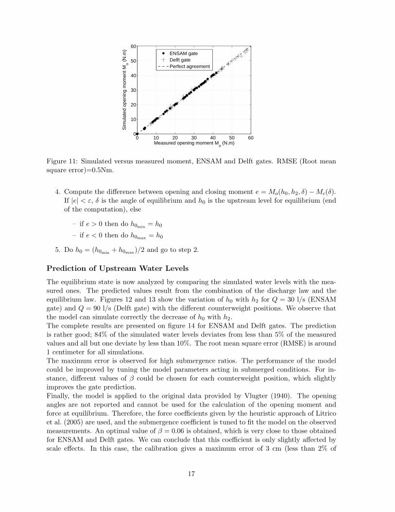
being independent on Φ. The calibrated values of these coefficients are given in table 2. Thecorrespondence between simulated and measured moments is excellent as shown on Fig. 11.

Full Model of the Vlugter Gate

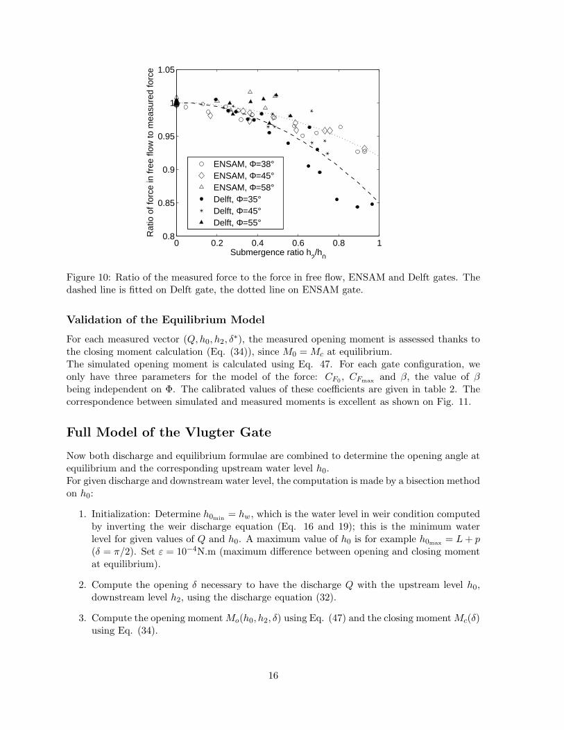
Now both discharge and equilibrium formulae are combined to determine the opening angle atequilibrium and the corresponding upstream water level h0.For given discharge and downstream water level, the computation is made by a bisection methodon h0:

1. Initialization: Determine h0min= hw, which is the water level in weir condition computed

by inverting the weir discharge equation (Eq. 16 and 19); this is the minimum waterlevel for given values of Q and h0. A maximum value of h0 is for example h0max

= L + p(δ = π/2). Set ε = 10−4N.m (maximum difference between opening and closing momentat equilibrium).

2. Compute the opening δ necessary to have the discharge Q with the upstream level h0,downstream level h2, using the discharge equation (32).

3. Compute the opening moment Mo(h0, h2, δ) using Eq. (47) and the closing moment Mc(δ)using Eq. (34).

16

0 10 20 30 40 50 600

10

20

30

40

50

60

Measured opening moment Mo (N.m)

Sim

ulat

ed o

peni

ng m

omen

t Mo (

N.m

)

ENSAM gateDelft gatePerfect agreement

Figure 11: Simulated versus measured moment, ENSAM and Delft gates. RMSE (Root meansquare error)=0.5Nm.

4. Compute the difference between opening and closing moment e = Mo(h0, h2, δ) −Mc(δ).If |e| < ε, δ is the angle of equilibrium and h0 is the upstream level for equilibrium (endof the computation), else

– if e > 0 then do h0min= h0

– if e < 0 then do h0max= h0

5. Do h0 = (h0min+ h0max

)/2 and go to step 2.

Prediction of Upstream Water Levels

The equilibrium state is now analyzed by comparing the simulated water levels with the mea-sured ones. The predicted values result from the combination of the discharge law and theequilibrium law. Figures 12 and 13 show the variation of h0 with h2 for Q = 30 l/s (ENSAMgate) and Q = 90 l/s (Delft gate) with the different counterweight positions. We observe thatthe model can simulate correctly the decrease of h0 with h2.The complete results are presented on figure 14 for ENSAM and Delft gates. The predictionis rather good; 84% of the simulated water levels deviates from less than 5% of the measuredvalues and all but one deviate by less than 10%. The root mean square error (RMSE) is around1 centimeter for all simulations.The maximum error is observed for high submergence ratios. The performance of the modelcould be improved by tuning the model parameters acting in submerged conditions. For in-stance, different values of β could be chosen for each counterweight position, which slightlyimproves the gate prediction.Finally, the model is applied to the original data provided by Vlugter (1940). The openingangles are not reported and cannot be used for the calculation of the opening moment andforce at equilibrium. Therefore, the force coefficients given by the heuristic approach of Litricoet al. (2005) are used, and the submergence coefficient is tuned to fit the model on the observedmeasurements. An optimal value of β = 0.06 is obtained, which is very close to those obtainedfor ENSAM and Delft gates. We can conclude that this coefficient is only slightly affected byscale effects. In this case, the calibration gives a maximum error of 3 cm (less than 2% of

17

0 0.2 0.4 0.6 0.8 10.1

0.15

0.2

0.25

0.3

0.35

0.4

submergence ratio h2/h

0

upst

ream

wat

er le

vel h

0 (m

)

ENSAM gate, Q=30 l/s

h0, weir formula

h0, measured values

h0, simulated values

Φ=38°Φ=43°

Φ=58°

Figure 12: ENSAM gate, simulated and measured upstream levels with respect to the submer-gence ratio h2/h0 – discharge = 30 l/s. RMSE=0.0106m.

0 0.2 0.4 0.6 0.8 10.25

0.3

0.35

0.4

0.45


0

upst

ream

wat

er le

vel h

0 (m

)

Delft gate, Q=90 l/s

h0, weir formula

h0, measured values


Φ=35° Φ=45°

Φ=55°

Figure 13: Delft gate, simulated and measured upstream levels with respect to the submergenceratio h2/h0 – discharge = 90 l/s. RMSE=0.009m.

18

0.1 0.15 0.2 0.25 0.3 0.35 0.4 0.45 0.50.1

0.15

0.2

0.25

0.3

0.35

0.4

0.45

0.5

measured h0 (m)

sim

ulat

ed h

0 (m

)

ENSAM gateDelft gateperfect agreement

Figure 14: Simulated versus measured upstream water level, ENSAM and Delft gates

the measured upstream level) between predicted and measured values (figure 15). Using thecoefficients obtained for Delft and ENSAM gates yields a larger error (7 cm, which correspondsto 5%) but still acceptable.

Prediction of Opening Angles at Equilibrium

The opening angles are correctly simulated in free flow. When the submergence ratio s increases,the gate opening increases due to the head-opening-discharge relationship. Fig. 8 showedlarger errors on the gate opening δ for large values of δ/δmax, due to the small sensitivity of thedischarge with respect to δ in this domain. The same discrepancy is observed when simulatingthe opening angle at equilibrium. This discrepancy is mainly due to the discharge relationship,since the model of the force is very accurate.Fig. 16 depicts the variation of δ∗ with the submergence ratio s = h2/h0. The simulated valuesresult from the complete calculation of h0 and δ∗. Again, it can be observed that the predictionis accurate unless for large angles (δ∗ close to δmax), which corresponds to large submergenceratios.

Discussion

The approach presented here is rather accurate to model the gate behavior in submergedconditions. Compared to free flow, the discharge formula needs to include a reduction factor S,expressed as a function of the submergence ratio h2/h0. This reduction factor uses calibratedcoefficients, but standard parameters gave satisfactory results on the studied gates.The effect of submergence on the force at equilibrium is simulated using a parameter β whichaccounts for the pressure field modification between free flow and submerged flow. The pressurefield implies modifications of the pressure force and on the lever arm position. Both effectscan be analyzed through the following non-dimensional numbers, characteristic of the gategeometries:

19

0 2.5 5 7.5 10 12.5 15 17.5 20−0.50

−0.25

0.00

0.25

0.50

0.75

1.00

1.25

1.50

1.75

2.00

discharge (m3/s)

Wat

er e

leva

tions

(m

)

Vlugter gate

h0, model

h0, Vlugter data

h2

Figure 15: Vlugter gate, original data – comparison of model and data

−0.4 −0.2 0 0.2 0.4 0.6 0.8 10

10

20

30

40

50

60

Submergence ratio h2/h

0

open

ing

angl

e at

equ

ilibr

ium

δ

* (de

g)

ENSAM gate, Φ = 38°

Q=60 l/s

Q=30 l/s

Q=10 l/s

simulated δmeasured δ

Figure 16: Simulated angle, ENSAM gate, Φ = 38◦. Due to gate oscillations, only one mea-surement is available for Q = 10 l/s; in this case, the predicted angle merges into the measuredone.

20

• r1 = hd/Bg, ratio of design upstream level to gate width: when r1 is large, the sideeffects are significant. In this case, the difference between the actual pressure field andthe hydrostatic field should be high. Larger values of β should be observed.

• r2 = hd

L , ratio of design water level to gate height: the lever arm La is determined bythe pressure field, although it is calculated like in hydrostatic conditions. Actually, theincertitude is all the higher as the water column on the upstream side of the gate is high,say r2 is close to 1. On the contrary, small values of r2 imply that La ≃ L whether thepressure field is hydrostatic or not.

These ratios are calculated for each studied gate (Table 3). Although the number of studiedsystems is not sufficient to establish quantitative relationships, we can observe a certain coher-ence in the correction factors β. The higher values of β correspond to Delft gate, where theside effects are significant (r1 high) and the design level is high (r2 high). The Vlugter gate israther wide and the side effect are negligible. In this case, we can observe a rather small valueof the correction factor β. ENSAM gate has slightly lower values of r1 and r2 than Delft gatewhich is consistent with the variation of β.

Table 3: Gate characteristics and β parameter

Gate Φ (deg) hd (m) Bg (m) L (m) r1 = hd/Bg r2 = hd/L β

Delft [35; 45; 55] 0.30 0.40 0.47 0.75 0.64 0.12ENSAM [38; 45; 58] [0.27;0.23;0.18] 0.38 0.42 [0.71;0.61;0.47] [0.64;0.55;0.43] 0.08Vlugter 45 1.15 6.00 1.50 0.19 0.77 0.06

Finally, the sensitivity to this parameter is analyzed (Fig. 17). The upstream water level issimulated for different values of β, from β = 0 (no effect of submergence taken into account)to β = 0.12 (value obtained for Delft gate). It can be observed that the upstream water levelcan decrease when h2 increases only when the effect of submergence on the force is taken intoaccount (β 6= 0). Exaggerated values of β exaggerate the decrease of h0, and lead to an errorof 3 centimeters at high submergence ratios (15%).

Conclusion

This paper derives a model of the Vlugter gate behaving under submerged conditions. Thedifficulty to model such systems is to simulate the transition regime between the undershotgate behavior (small gate opening) and the weir behavior (large opening).The proposed model combines a discharge law, based on the interpolation between a under-shot gate behavior and a weir behavior, and an equilibrium law based on the trajectory atequilibrium of the force exerted on the gate.The discharge formula was validated on two small-scale gates and comprises only two classicalparameters (discharge coefficients for an undershot gate and a broad-crested weir). This formulacan be applied to any rectangular flap gate.In free flow, the equilibrium relationship uses two parameters depending on the position ofthe center of gravity. To take account of the submergence effect, one tuning parameter isintroduced.Coupling the discharge law with the equilibrium law, the model is able to accurately simulatethe upstream water level h0 and the gate opening at equilibrium δ∗ for a given discharge Qand a downstream water level h2.

21

0 0.2 0.4 0.6 0.8 1

0.2

0.25

0.3

0.35

0.4


0

upst

ream

wat

er le

vel h

0 (m

)

ENSAM gate, Q=30 l/s, Φ=38°

h0, measured values


β=0

β=0.06 β=0.08

β=0.12

Figure 17: ENSAM gate, Φ = 38◦; influence of parameter β on simulated water levels

The model has been validated on a set of data collected on two small-scale gates, and on theoriginal Vlugter gate data (Vlugter, 1940), with a very satisfying result. This model enablesto accurately predict the stationary behavior of the gate.The proposed model could be used to evaluate the impact of design parameters on the gateperformance in terms of water level control.

Acknowledgements

The experimental setup was built by Paul Oullier and Gerard Alvarez, technical assistants ofthe hydraulic laboratory of ENSAM, whose help is gratefully acknowledged. We would alsolike to thank Prof. R. Brouwer from Delft University of Technology who kindly provided thedata from de Graaff’s master’s thesis.

Appendix

Interpolation of a Cubic Curve

Let f(δ) denote the function defined for δ ∈ [0, δw] that verifies the following interpolationconditions:

• f(0) = f0,

• f(δw) = fw,

• dfdδ (0) = df0,

• dfdδ (δw) = dfw.

where f0, fw, df0, dfw are real numbers giving the values of the function and its derivative at0 and δw.

22

f(δ) is parameterized as a cubic polynomial:

f(δ) = c0 + c1δ + c2δ2 + c3δ

3

The four interpolation conditions provide a linear system of four equations. Solving for c0, c1,c2 and c3 gives:

c0 = f0 (48)

c1 = df0 (49)

c2 = 3fw − f0

δ2w

− 2df0 + dfw

δw(50)

c3 = 2f0 − fw

δ3w

+df0 + dfw

δ2w

(51)

Notations

The following notations are used in this paper:β = correction factor on the force at equilibriumδ = angle of opening (rad)δw = angle of opening corresponding to the flow over the weir (rad)δmax = maximum angle of opening corresponding to the unstable equilibrium (rad)Φ = angle (Ox,OG) (rad)ρ= density of water (1000 kg/m3)Bc = canal width, downstream pool (m)Bg = gate width (m)Bw = weir width (m)CF0

: tuning coefficientCFmax

: tuning coefficientCc : contraction coefficientCu : discharge coefficient for the flow under the gateCw, Cw0

: Weir discharge coefficientF = opening force (N)g = gravitational acceleration (9.81 m/s2)H0 = upstream head (m)H2 = downstream head (m)h0 = upstream water level (m)h1 = hydrostatic head in the contracted section (m)h2 = downstream water level (m)hd = design upstream water level (m)hwu = upstream height of the weir (m)hwd = downstream height of the weir (m)hw = upstream water level in weir behavior (m)L = gate height (m)La = lever arm for the opening moment calculation (m)Lw : weir length (m)MG = mass of the gate without counterweight (kg)MW = mass of the counterweight (kg)M = MW + MG = total mass of the gate and counterweight (kg)

23

Mo = opening moment (Nm)Mc = closing moment (Nm)p = lever arm from hinge point to gate (m)Q = total discharge (m3/s)Qr = residual discharge at δ = 0 (m3/s)Qw = discharge in weir position (m3/s)Qwf = discharge in weir position, free flow (m3/s)Qside = side discharge (m3/s)Qunder = discharge under the gate (m3/s)r1 = hd/Bg = ratio of design upstream level to gate widthr2 = hd

L , ratio of design water level to gate heights = h2/h0 = submergence ratioSw = Qw/Qwf = correction factor on the weir discharge, due to submergenceU = gate opening (m)Uh = horizontal gate opening (m)Uv = vertical gate opening (m)Vu = mean velocity at the brink (m/s)x= horizontal distance from the weir downstream brink (m)XG = horizontal distance of the center of gravity from the pivot point (m)yL = modular limit of a weir (maximum value of s for free flow)ZG = vertical distance of the center of gravity from the pivot point (m)z = vertical distance from the weir crest (m)ENSAM = Ecole Nationale Superieure Agronomique de MontpellierHVIP = Hadejia Valley Irrigation Project

References

Bos (1989). Discharge measurement structures. 3rd edition, ILRI, Wageningen, The Nether-lands

Brants, M. (1996). Automatic gates facilitate water management in Punggur Utara irrigationproject. In ICID, editor, 16th International Congress on Irrigation and Drainage, Cairo,Egypt.

Burt, C., Angold, R., Lehmkuhl, M., and Styles, S. (2001). Flap gate design for automaticupstream canal water level control. J. of Irrigation and Drainage Engineering, 127(2):84–91.

Brouwer, R. (1987). Design and application of automatic check gate for tertiary turnouts. In13th ICID Congress, pages 671–683, Rabat, Morroco.

Cunge, J.A., Holly, F.M., Vervey, A. (1980). Practical aspects of computational river hydraulics.Pitman. 420p.

Davis, A., Jacob, P., and Ellett, G. (1999). Estimating trajectory of free overfall nappe. J. of

Hydraulic Engineering, 125(1):79–82.

de Graaff, B. (1998). Stability analysis of the Vlugter gate. Master’s thesis, Delft Universityof Technology, Faculty of Civil Engineering and Geosciences.

24

Hager, W. (1983). Hydraulics of plane free overfall. J. of Hydraulic Engineering, 109(12):1683–1697.

Hager, W. and Schwalt, M. (1994). Broad-crested weir. J. Irrig. Drain. Engrg, 109(12):1683–1697.

Litrico, X., Belaud, G., Baume, J.-P., and Ribot-Bruno, J. (2005). Hydraulic modeling of anautomatic upstream water-level control gate. J. Irrig. Drain. Engrg., 131(2):176–189.

Sinniger, R. and Hager, W. (1989). Constructions hydrauliques. Traite de Genie Civil, Vol.15. Presses Polytechniques Romandes, 439p. (in French).

Vlugter, H. (1940). Over zelfwerkende peilregelaars bij den waterstaat in nederlandsch-indie.De ingenieur in Nederlandsch-Indie, (6):84–93. (in Dutch).

USDA (1973). Submerged weir flow. Soil Conservation Service, design note No 15

25

Hydraulic Modeling of an Automatic Upstream Water Level Control Gate for Submerged Flow Conditions

Documents

Transcript of Hydraulic Modeling of an Automatic Upstream Water Level Control Gate for Submerged Flow Conditions