Fuzzy Sets and Systems 159 (2008) 821–845www.elsevier.com/locate/fss

Hybridization of intelligent techniques and ARIMA models for timeseries prediction

O. Valenzuelaa, I. Rojasb,∗, F. Rojasb, H. Pomaresb, L.J. Herrerab, A. Guillenb,L. Marqueza, M. Pasadasa

aDepartment of Applied Mathematics, University of Granada, SpainbDepartment of Computer Architecture and Computer Technology, University of Granada, Spain

Received 17 February 2006; received in revised form 31 October 2007; accepted 4 November 2007Available online 17 November 2007

Abstract

Traditionally, the autoregressive moving average (ARMA) model has been one of the most widely used linear models in time seriesprediction. Recent research activities in forecasting with artificial neural networks (ANNs) suggest that ANNs can be a promisingalternative to the traditional ARMA structure. These linear models and ANNs are often compared with mixed conclusions in termsof the superiority in forecasting performance. In this paper we propose a hybridization of intelligent techniques such as ANNs, fuzzysystems and evolutionary algorithms, so that the final hybrid ARIMA–ANN model could outperform the prediction accuracy ofthose models when used separately. More specifically, we propose the use of fuzzy rules to elicit the order of the ARMA or ARIMAmodel, without the intervention of a human expert, and the use of a hybrid ARIMA–ANN model that combines the advantages ofthe easy-to-use and relatively easy-to-tune ARIMA models, and the computational power of ANNs.© 2007 Elsevier B.V. All rights reserved.

Keywords: Time series; ARIMA models; Fuzzy systems; Neural networks; Hybrid system

1. Introduction

When modelling linear and stationary time series, the researcher frequently chooses the class of autoregressivemoving average (ARMA) models because of its high performance and robustness [6]. The ARMA(p, q) model for atime series can be expressed as

xt =p∑

i=1

�ixt−i −q∑

j=1

�j et−j + et , (1)

where et is a normal white noise process with zero mean and variance �2, and t = 1, . . . , T , T being the number ofdata of the time series. It is assumed that the autoregressive and moving average parameters satisfy the conditions forstationarity and invertibility, respectively. Since the moving average component of Eq. (1) is assumed to be invertible,

∗ Corresponding author. Tel.: +34 958 246128; fax: +34 958 248993.E-mail address: irojas@atc.ugr.es (I. Rojas).

0165-0114/$ - see front matter © 2007 Elsevier B.V. All rights reserved.doi:10.1016/j.fss.2007.11.003

822 O. Valenzuela et al. / Fuzzy Sets and Systems 159 (2008) 821–845

Eq. (1) can be rewritten as an infinite order autoregression in the form:

xt =∞∑i=1

�ixt−i + et . (2)

In order to implement the equation, the autoregression is truncated to a finite order, say R, being R < T , and ignoringthe error induced by the truncation gives

xt =R∑

i=1

�ixt−i + et . (3)

Eq. (3) can be estimated by OLS to obtain estimates of �i , �i , et and et , where

et = xt −R∑

i=1

�ixt−i . (4)

These estimates of the innovation series et and et can be substituted into Eq. (1), and therefore the time series can bemodelled as

xt =p∑

i=1

�ixt−i −q∑

j=1

�j et−j + �t , (5)

where �t = et −∑qj=1 �j (et−j − et−j ).

The main advantage of ARMA forecasting is that it only requires data of the time series in question. First, thisfeature is advantageous if we are forecasting a large number of time series. Second, this avoids a problem that occurssometimes with multivariate models: for example, consider a model including wages, prices and money. It is possiblethat a consistent money series is only available for a shorter period of time than the other two series, restricting the timeperiod over which the model can be estimated. Third, with multivariate models, timeliness of data can be a problem.If one constructs a large structural model containing variables which are only published with a long lag, such as wagedata, then forecasts using this model are conditional forecasts based on forecasts of the unavailable observations, addingan additional source of forecast uncertainty.

Different order selection methods based on validity criteria, based on the information-theoretic approaches such asthe Akaike’s information criterion (AIC) or with other model selection techniques like minimum description length(MDL) have been proposed in [24,29,35,55]. The selection of a particular ARMA model, however, is neither easy norwithout implications for the goal of the analysis.

In fact, in [20] it is noted that for time time-varying model identification, the optimal model structure is not easyto determine, so that it is difficult to apply the AIC or MDL criteria, which often leads to failure in selecting asuitable model order. Therefore, different approaches based on intelligent paradigms, such as neural networks, ge-netic algorithms or fuzzy system have been proposed to improve the accuracy of order selection of ARIMA models[63,74,25,20,39,42,41,31,13,8,14]. It is important to note that, nowadays, the most used and commercial tools for timeseries forecasting (Statgraphics, SPSS, etc.) require the intervention of a human expert for the definition of the ARMAmodel or the specification of the types of model to be fitted to the time series (X-12-ARIMA). Some other problemswhich arise when forecasting with ARMA models are:

• The result of the Box–Jenkins procedure depends greatly on the competence and experience of the expert researchersand is affected by a strong path-dependence [66]. Unfortunately, one frequently observes that different models havesimilar estimated correlation patterns, and the choice among competitive models can be quite arbitrary. Some concernderives also from comparative studies in which experts, asked to identify a number of time series, frequently reachdifferent conclusions [6,10,56].

• A further objection to the Box–Jenkins procedure for model selection is related to the time required to develop theidentification model, which sometimes can be excessively high.

• It is not embedded within any underlying theoretical model or structural relationships. Furthermore, it is not possibleto run policy simulations with ARMA models, unlike with structural models

• ARMA models are linear models but, in the real-word time series are rarely pure linear combinations.

O. Valenzuela et al. / Fuzzy Sets and Systems 159 (2008) 821–845 823

The existence of these disadvantages together with the advance of artificial intelligence techniques, have stimulatedthe development of new alternative solutions to time series forecasting. Two of the forecasting techniques that allowfor the detection and modelling of nonlinear data are rule induction [46,27,21,44] and neural networks [57,47,51].Rule induction identifies patterns in the data and expresses them as rules. Expert systems are an example of use of thistechnique. On the other hand, neural networks present an important class of nonlinear prediction model family that hasgenerated considerable interest in the forecasting community in the past decade. The main advantage of this modellingparadigm lies on the universal approximation property, i.e., neural networks could approximate any continuous functiondefined on a compact set with arbitrary precision. The model parameters are iteratively adjusted and optimized throughnetwork learning of historical patterns. One of the best known neural network models is the multi-layer feed-forwardneural network, called the multi-layer perceptron (MLP), consisting of an input layer, one or several hidden layers andan output layer. Nevertheless, it is worth mentioning that ARMA models are still the benchmark against which theeffectiveness of the new proposed methodologies are tested [63,65,15,1,25].

In fact, it is important to note the comparative study of back-propagation networks versus ARMA models on selectedtime series data from the well-known M-competition [36] performed by Tang et al. [57]. It was concluded that neuralnetworks not only could provide better long-term forecasting but also did a better job than ARMA models when givenshort series of input data. Also, the same authors in Tang and Fishwich [58] conducted a more comprehensive study ofback-propagation neural network’s ability to model time series. In [58] 14 time series data sets from the well-knownM-competition plus two additional airlines and sales data sets were used, with the conclusion that ANNs perform betterthan Box–Jenkins models for more irregular series and for multiple-period-ahead forecasting.

In [22] 104 time series data sets from the same M-competition were used and compared the performance of ANNswith that of six other traditional statistical models including the Box–Jenkins’ ARMA model. They found that ANNsperformed considerably better than the six traditional methods for monthly and quarterly time series while Box–Jenkinsmodel was comparable to neural networks for annual time series. When linearity or nonlinearity was considered, theyconcluded that the neural-network model was significantly better than the reference average. However, it was unclearhow the neural-network model behaved compared with the Box–Jenkins model for these linear time series. This againmotivated us to carry out the proposed study.

Although the application of neural network modelling to Box–Jenkins models encompasses two sub-areas, that is,model identification (by a statistical feature extractor, perform a pattern classification) and forecasting (as a functionapproximator), the scope of this paper will be focused on both areas, but using a fuzzy expert system for automaticmodel identification.

The organization of the rest of the paper is the following: the next section will explain in detail the fuzzy expertsystem, which is optimized by an evolutionary algorithm, to obtain in an autonomous way the structure of the ARIMAtime series. Section 3 presents the hybrid methodology that combines the linear time series obtained in Section 2 andan ANN model, represented by a MLP, for time series forecasting. Section 4 presents the simulation results and Section5 the main conclusion of the presented methodology.

2. Fuzzy expert system: the structure of the ARIMA model

In Section 1, we have reported several justifications for an automatic ARMA model building procedure. They canbe summarized by saying that using the Box–Jenkins method on a large scale requires both expertise and time. Aimingto make the method available to people without that expertise, several software vendors have implemented automatedtime series forecasting methods, e.g. Mandrake [3], and the list in Tashman [59]. However, these approaches werenot very successful and nowadays, most popular statistical package (SPSS, Statgraphics, Matlab, etc.), require theintervention of the user. There are also other software packages that perform automatic model selection with minorintervention of an expert system (as STSA toolbox [71] or X-12-ARIMA software [72]). For example, in the X-12-ARIMA software, the user has to specify which types of models are to be fitted to the time series in a procedure in whichthese different models are sequentially selected and evaluated. To determine whether or not a model fits the data well,the Portmanteau test of fit developed by Box and Pierce [7] with the variance correction for small samples introducedby Ljung and Box [34] is used, and in a final file, all the different models selected by the user expert are evaluated.The null hypothesis of randomness of the residuals is tested at a 5% level of significance and the estimated parameters arechecked to avoid over-differencing. Additionally, in order to effectively and easily identify the order of ARIMA, somepattern identification methods have been proposed, including the R and S array method [68], the Corner method [5],

824 O. Valenzuela et al. / Fuzzy Sets and Systems 159 (2008) 821–845

the ESACF method [61], the SCAN method [62] and the MINIC method [19]. Although these identification methodsseem to provide a better method for determining the order of the ARIMA model, there are some problems which requireconsideration [10]. In fact, most of them require the interpretation of a human expert for a clear identification of theARIMA model, they cannot be used for seasonal time series model, and these methods provide only local optimumsolutions.

In [20] it is noticed that in order to improve the accuracy of the order selection of an ARMA model, it is possibleto effectively use knowledge learned from experience. Because this knowledge is usually vaguely expressed, fuzzysystems provide the capability to express subjective and vague objects in an inference engine [45,52,64].

The goal of this section is to present an automated way to obtain the structure of an ARIMA model, using an expertsystem working with fuzzy logic. On many occasions, a series is not exclusively fitted to one model, but rather variousmodels may equally well fit the series [57]. If we follow the norms of Box and Jenkins, the model chosen is nearlyalways the simplest one, i.e. the one involving fewest terms [2].

The method is carried out in the following way: the time series of a model must fulfil a set of rules. Given such arule set, and a time series to be analysed, we measure how many rules are fulfilled by the series. Based on the degreeof fulfilment of these rules, we can elicit which is the suitable model for that time series.

Now, we have to be careful with one important issue: the number of rules fulfilled for a certain ARMA model shouldnot be the only measure to take into account. Let us suppose that the AR(1) model is associated with two fuzzy rules,and that the ARMA(1,1) model is associated with six. It may occur that for a real AR(1) model, three out of the sixARMA(1,1) rules are satisfied. In this case, the method could mistakenly associate the series with an ARMA(1,1) modelinstead of the true AR(1) model. Therefore, the methodology proposed in this section will try to maintain a number ofrules as similar as possible for every model, and also will assign weights to every rule. Thus, the degree of fulfilmentof a model will depend on the sum of weights of the rules that a time series satisfies.

Finally, another difficult task we will be dealing with in this section is to propose an algorithm capable of assigningweights to each fuzzy rule so that all time series analysed can be correctly identified. This, as we will see later, will beaccomplished with the aid of an evolutionary algorithm.

2.1. Pre-processing the time series

It is important to note, that in order to obtain the linear model of a time series, the first step is to determine if a naturallog transformation of the series is necessary. This step is accomplished using the likelihood ratio. It is necessary to takeinto account that the likelihood is greater for the transformed series than the raw series when

log

⎛⎝1

n

∑i

(log(Yi) − 1

n

∑i

log(Y )

)2⎞⎠ >

(log

(1

n

∑i

(Yi − Y )2

)+ 2

n

∑i

log(Yi)

). (6)

If the inequality is fulfilled, it is necessary to take the log transform.On the other hand, the univariate Box–Jenkins ARMA method applies only to stationary time series. In time series

analysis, a stationary series has a constant mean, variance and autocorrelation through time, i.e., serial or seasonaldependencies have been removed (the formal definition of stationary is more complicated, but the definition given hereis adequate for the present purposes). Serial dependency can be removed by differentiating of differencing the series,that is to say, converting each element of the series into its difference from the previous one. There are two majorreasons for such transformations: First, the hidden nature of serial dependencies in the series can be thus identified andsecond, it is necessary for the Box–Jenkins methodology.

Therefore, for an ARIMA(p, d, q) model, it is necessary to obtain the (p, d, q) parameters, where p is the numberof autoregressive terms, d is the number of non-seasonal differences and q is the number of lagged forecast errors inthe prediction equation. The first step is to identify the order of differencing needed to make the series stationary (inconjunction with a previous variance-stabilizing transformation such as taking logs or deflating, as presented in Eq. (6)).Most economic (and also many other) time series do not satisfy the stationarity conditions stated earlier for whichARMAmodels have been derived. Then these times series are called non-stationary and should be re-expressed so that theybecome stationary with respect to the variance and the mean, selecting the appropriate value of parameter d.

O. Valenzuela et al. / Fuzzy Sets and Systems 159 (2008) 821–845 825

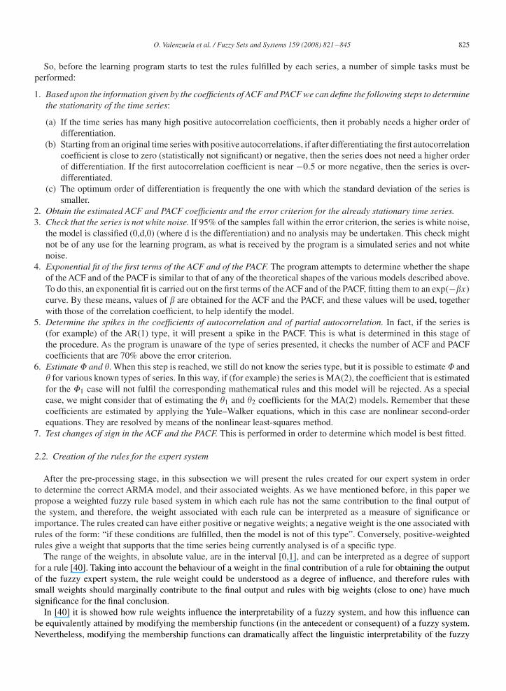
So, before the learning program starts to test the rules fulfilled by each series, a number of simple tasks must beperformed:

1. Based upon the information given by the coefficients of ACF and PACF we can define the following steps to determinethe stationarity of the time series:

(a) If the time series has many high positive autocorrelation coefficients, then it probably needs a higher order ofdifferentiation.

(b) Starting from an original time series with positive autocorrelations, if after differentiating the first autocorrelationcoefficient is close to zero (statistically not significant) or negative, then the series does not need a higher orderof differentiation. If the first autocorrelation coefficient is near −0.5 or more negative, then the series is over-differentiated.

(c) The optimum order of differentiation is frequently the one with which the standard deviation of the series issmaller.

2. Obtain the estimated ACF and PACF coefficients and the error criterion for the already stationary time series.3. Check that the series is not white noise. If 95% of the samples fall within the error criterion, the series is white noise,

the model is classified (0,d,0) (where d is the differentiation) and no analysis may be undertaken. This check mightnot be of any use for the learning program, as what is received by the program is a simulated series and not whitenoise.

4. Exponential fit of the first terms of the ACF and of the PACF. The program attempts to determine whether the shapeof the ACF and of the PACF is similar to that of any of the theoretical shapes of the various models described above.To do this, an exponential fit is carried out on the first terms of the ACF and of the PACF, fitting them to an exp(−�x)

curve. By these means, values of � are obtained for the ACF and the PACF, and these values will be used, togetherwith those of the correlation coefficient, to help identify the model.

5. Determine the spikes in the coefficients of autocorrelation and of partial autocorrelation. In fact, if the series is(for example) of the AR(1) type, it will present a spike in the PACF. This is what is determined in this stage ofthe procedure. As the program is unaware of the type of series presented, it checks the number of ACF and PACFcoefficients that are 70% above the error criterion.

6. Estimate � and �. When this step is reached, we still do not know the series type, but it is possible to estimate � and� for various known types of series. In this way, if (for example) the series is MA(2), the coefficient that is estimatedfor the �1 case will not fulfil the corresponding mathematical rules and this model will be rejected. As a specialcase, we might consider that of estimating the �1 and �2 coefficients for the MA(2) models. Remember that thesecoefficients are estimated by applying the Yule–Walker equations, which in this case are nonlinear second-orderequations. They are resolved by means of the nonlinear least-squares method.

7. Test changes of sign in the ACF and the PACF. This is performed in order to determine which model is best fitted.

2.2. Creation of the rules for the expert system

After the pre-processing stage, in this subsection we will present the rules created for our expert system in orderto determine the correct ARMA model, and their associated weights. As we have mentioned before, in this paper wepropose a weighted fuzzy rule based system in which each rule has not the same contribution to the final output ofthe system, and therefore, the weight associated with each rule can be interpreted as a measure of significance orimportance. The rules created can have either positive or negative weights; a negative weight is the one associated withrules of the form: “if these conditions are fulfilled, then the model is not of this type”. Conversely, positive-weightedrules give a weight that supports that the time series being currently analysed is of a specific type.

The range of the weights, in absolute value, are in the interval [0,1], and can be interpreted as a degree of supportfor a rule [40]. Taking into account the behaviour of a weight in the final contribution of a rule for obtaining the outputof the fuzzy expert system, the rule weight could be understood as a degree of influence, and therefore rules withsmall weights should marginally contribute to the final output and rules with big weights (close to one) have muchsignificance for the final conclusion.

In [40] it is showed how rule weights influence the interpretability of a fuzzy system, and how this influence canbe equivalently attained by modifying the membership functions (in the antecedent or consequent) of a fuzzy system.Nevertheless, modifying the membership functions can dramatically affect the linguistic interpretability of the fuzzy

826 O. Valenzuela et al. / Fuzzy Sets and Systems 159 (2008) 821–845

system. In [60], a genetic algorithm is proposed to tune a weighted fuzzy rule-based system. In this approach theparameters defining the membership functions, including position and shape of the fuzzy rule set and weights of rulesare evolved jointly using a genetic algorithm, obtaining successful results in classification problems. In [11] a newmethod to estimate null values in relational database systems using genetic algorithms is proposed, where the attributesappearing in the antecedent parts of the generated fuzzy rules have different weights. A similar approach, but using aneural network is presented in [17], to generate weighted fuzzy rules. In this method, through analysis of the weightsof neural network, it is possible to obtain a matrix of importance indices that indicates the influential power of eachinput node in determining the output for each output node. Therefore weighted fuzzy rules are extracted from the neuralnetwork. However, in the kind of fuzzy rule weighting proposed in [17] the number of parameter to be optimized isvery high (one weight not for one rule, but for all the membership functions in the antecedent of each rule) and thelinguistic interpretation of the final fuzzy system is not preserved.

The expert system that is created consists of a total of 38 fuzzy rules (Table 1) using the Mamdani inference model.There exist many possibilities to select the set of basic operations in the fuzzy inference process. Thus, there are severalalternatives for the defuzzifier, to define the fuzzy implication operators, to select the conjunction and disjunctionoperators, the set of membership functions to be used in the definition of the linguistic variables, etc. [48,49]. In thispaper, the fuzzy inference method uses the minimum as T-norm and the centroid method as the defuzzification strategy,and the type of membership function was triangular functions [50].

For example, analysing Table 1, the first two rules are defined for simple or pure AR/MA models. In fact, the ACFand PACF make it available some assistance on how to select pure AR or pure MA models. However, rule 3 is dedicatedto mixture models, which are much harder to identify: RULE 3. If both PACF and ACF fall with the same abruptness,the model is ARMA(P, Q), being P and Q the number of PACF and ACF coefficients above the error criterion. Thisrule is suggested by the shape of the AR models and MA models. In pure AR models, the ACF falls smoothly, while thePACF falls abruptly. In pure MA models, the PACF falls smoothly, while the ACF falls abruptly. The number of PACF(ACF) coefficients above the error criterion will be the order of the pure AR model (pure MA model). To determinethis, the program uses the previously obtained � values of the exponential fit. The exponential presenting the mostabrupt change is the one with the highest absolute � value, such that if the � calculated for the PACF is greater thanthat for the ACF, the model will be AR (for MA, if the � calculated for the ACF is greater than that for the PACF, themodel will be MA). To determine the order, we examine the number of spikes in the PACF and ACF. As the series arenot ideal, but have a component of white noise, we only take into consideration the PACF and ACF that are 70% abovethe error criterion.

2.3. Optimization of the fuzzy logic rules

In this paper we use a genetic algorithm to optimize just only the weight associated to each fuzzy rule of the expertsystem. The behaviour of a genetic algorithm can be briefly described as: evaluate a population and generate a new oneiteratively, with each successive population referred to as a generation. Given the current generation at iteration t, G(t),the GA generates a new generation, G(t + 1), based on the previous generation, applying a set of genetic operations.

Given an optimization problem, simple GAs encode the parameters concerned into finite bit strings, and then runiteratively using genetic operators in a random way but based on the fitness function evolution to perform the optimizationtask. Note that the necessity for binary encoding of the parameters required is a controversial issue [16,23,69]. Theproblem existing in binary coding lies in the fact that a long string always occupies space in the computer memoryeven though only a few bits are actually involved in the crossover and mutation operations. This is particularly thecase when a lot of parameters need to be adjusted in the same problem and a higher precision is required for thefinal result [23]. It has been shown that real-encoded GAs converge faster, the results are more consistent and higherprecision can be achieved, especially for larger problems where binary representation becomes prohibitively longand search time increases as well. This paper is concerned with real number representation [16], which in principleseems more favourable for optimizing the parameters of the rule weight of the fuzzy system, which are defined in acontinuous domain [54,33]. Therefore, the parameters of each weighted fuzzy rule are encoded in a chromosome as areal vector.

Typical crossover and mutation operators have been used for the manipulation of the current population in everyiteration of the GA. The crossover operator is “simple one-point crossover”. the mutation operator is “non-uniformmutation” [38]. This operator presents the advantage, when compared to the classical uniform mutation operator,

O. Valenzuela et al. / Fuzzy Sets and Systems 159 (2008) 821–845 827

Table 1Rules used by the expert system for the ARMA model structure

1. If the PACF fall more abruptly than the ACF, then the model is AR(P ), being P the number of PACF above the error criterion2. If the ACF fall more abruptly than the PACF, then the model is MA(Q), being Q the number of ACF above the error criterion3. If both PACF and ACF fall with the same abruptness, the model is ARMA(P, Q), being P and Q the number of PACF and ACF

coefficients above the error criterion4. If the ACF are discontinued suddenly, the process is MA(Q), where Q is the number of ACF above the error criterion5. If both PACF and ACF fall with exactly the same abruptness, the model is ARMA(1,1)6. If the number of coefficients above the error criterion in the ACF is less than in the PACF, the model is MA(Q), where Q is the

number of ACF coefficients above the error criterion7. If the number of coefficients above the error criterion in the PACF is less than in the ACF, the model is MA(Q), where Q is the

number of PACF coefficients above the error criterion8. If the number of coefficients above the error criterion in the ACF is equal than the number of coefficients above the same criterion

in the PACF, the series is ARMA(P, Q), being P and Q the number of PACF and ACF coefficients above the error criterion,respectively

9. If the ACF sign changes, the series is AR(3)10. If the correlation coefficient of the ACF is greater than the PACF, the model is AR(1)11. If the estimated �1 coefficient for the AR(1) model fulfils the stationary conditions, the series is AR(1)12. If the series is AR(1), the first estimated correlation coefficient will be approximately equal to the first estimated partial autocor-

relation coefficient13. If the estimated �1 coefficient is positive and the PACF peak is positive, the series is AR(1)14. If the estimated �1 coefficient is negative and the PACF peak is negative, the series is AR(1)15. If the � from the PACF exponential adjustment is zero, the series is AR(1)16. If the estimated �1 coefficient for the model fulfils the invertibility requirements, the series is MA(1)17. If only the first autocorrelation coefficient is not null, the series is MA(1)18. If the estimated �1 coefficient is negative, the ACF peak is positive and the PACF change the sign starting from the positive sign,

the process is MA(1)19. If the estimated �1 coefficient is positive, the ACF peak is negative and the PACF do not change the sign starting from the negative

sign, the process is MA(1)20. If the � from the ACF exponential adjustment is zero, the series is MA(1)21. If the estimated �1 and �2 coefficients fulfil the stationary conditions, then the series is AR(2)22. If the series is AR(2), the two first autocorrelation coefficients must fall within the area enclosed by the following curves:

|rk1| < 1, |rk2| < 1, r2k1 < 1

2 (rk2 + 1)

23. If the ACF change theirs sign, the process is AR(2)24. If there are only two PACF with absolute value above the error criterion, the process is AR(2)25. If the estimated �1 and �2 coefficients fulfil the invertibility conditions, then the process is MA(2)26. If there are only two ACF with absolute value above the error criterion, the process is MA(2)27. If the model is MA(2), rk1 and rk2 must fall within the area enclosed by:

rk1 + rk2 = −0.5, rk2 − rk1 = −0.5, r2k1 = 4rk2(1 − 2rk2)

28. If the PACF change theirs sign, the process is MA(2)29. If the estimated �1 and �1 coefficients fulfil the stationary and invertibility conditions, then the series is ARMA(1,1)30. If rules 11 and 16 are fulfilled, the model is ARMA(1,1)31. If rule 11 is not fulfilled, the series is not AR(1)32. If rule 16 is not fulfilled, the series is not MA(1)33. If rule 21 is not fulfilled, the series is not AR(2)34. If rule 25 is not fulfilled, the series is not MA(2)35. If rule 29 is not fulfilled, the series is not ARMA(1,1)36. If the probability of the series to be an AR(P ) is high and the probability to be an MA(Q) is small, then the series is AR(P )

37. If the probability of the series to be an MA(Q) is high and the probability to be an AR(P ) is small, then the series is MA(Q)

38. If the probability of the series to be an AR(P ) is high and the probability to be an MA(Q) is high, then the series is ARMA(P, Q)

of performing less significant changes to the genes of the chromosome as the number of generations grows. Thisproperty makes the exploration-exploitation trade-off be more favourable to exploration in the early stages of thealgorithm, while exploitation takes more importance when the solution given by the GA is closer to the optimalsolution.

An important function block for the behaviour of the genetic algorithm is the definition of the fitness function. Thefunction fitness f (x) evaluates each chromosome (possible solution) in the population, and test if the end condition issatisfied. The fitness function is responsible for guiding the search towards the global optimum. For this purpose, it must

828 O. Valenzuela et al. / Fuzzy Sets and Systems 159 (2008) 821–845

be designed to be able to compare two different individuals in order to distinguish the better solutions from the others.In our approach, the fitness function is the sum of the different errors in the estimation of the ARIMA structure, for thedifferent time series used. Mathematically, the fitness function, for a chromosome P in the generation t, is obtained as:

fitness(P t ) = 1∑Ni=1 ‖ARIMAi (pR, dR, qR) − ARIMAi (pE, dE, qE)‖ +

= 1∑Ni=1

√(pi

R − piE)2 + (di

R − diE)2 + (qi

R − qiE)2 +

, (7)

where is a constant required to avoid an infinite result with zero distances, ARIMAi (pR, dR, qR)R is the real ARIMAmodel for the time series iand ARIMAi (pE, dE, qE)E is the estimated models obtained with the fuzzy expert systemproposed, and ‖.‖ is the Euclidean distance, that evaluates the distance between both models. If various models arepossible for a given series, we test whether the one assigned the highest weight is at the lowest distance from the realresult. If so, there is no penalization, but otherwise what is stored is the average of the distances of the possible modelsfrom reality. Therefore, the fitness function adds the errors in the estimation of the structure of the ARIMA model foreach of the time series used in the training set.

Finally, in order to stop the genetic algorithm different criteria can be used. The most popular and easier criterionis the number of generations. Different analyses have been presented in the literature to determine a threshold forthe maximum number of generations [9]; however, all of these studies are based on binary-encoded representation.Furthermore, all of these criteria select a maximum number of generations, number that used to be very big. In thispaper, we have used a stop criterion based on the evolution of the fitness function, which allows the evolution to continueif the slope of the regression straight line of the last v0 generations is bigger than a certain value smin. The straight lineof the last v0 generation for the fitness function of the best solution obtained can be computed as

slope(v0) =∑t

k=t−v0+1(k − t)fitnessbest(Pk) −

(∑tk=t−v0+1 fitnessbest(P

k)) (∑t

k=t−v0+1 k − t)

v0∑tk=t−v0+1(k − t)2 −

(∑tk=t−v0+1 k − t

)2v0

, (8)

where fitnessbest(Pk) is the best fitness of the population in the generation k. Finally, it is important to note that in order

to obtain good generalization results, a large quantity of real series will be used as benchmarks in the prediction of timeseries (http://www.secondmoment.org/time_series.php). The results obtained for the simulations, except in the case ofthe mixed series, were highly promising and therefore, this ARIMA(p, d, q) structure will be used in conjunction withthe neural network.

3. The hybrid ARIMA–ANN approach

In this section time series decomposition is proposed in which ARIMA models and ANNs are combined in order toobtain a robust and efficient methodology for time series forecasting.

Several time series decomposition methods have been presented in the literature, (simple moving averages, centredmoving or weighted moving averages, local regression smoothing, additive or multiplicative decomposition, etc.)[4,12,18,37], which are mainly based on the following equation:

Yt = Patternt + Errort = f (trend − cycle, seasonality, error). (9)

In this approach, the first steps consist in removing the trend-cycle, and then isolate the seasonal component. The erroror residual cannot be predicted, but can be identified. Although this decomposition approach has several theoreticalweaknesses from a mathematical point of view, however, practitioners have largely uncared for these weaknesses andhave used the methodology with significant success. It is important to note that the time series decomposition methodsbased on Eq. (9) use a linear mathematical model, being the X-12-ARIMA software developed by Findley et al. in1997 [18] a very well-known tool.

As we have stated in Section 1, there exist many works in the literature that have tried to compare the performance ofANNs against linear models for a wide range of time series. The conclusion is that we cannot determine a priori whichmethod will be best suited to our series, since in some cases ANNs show a clear superiority but in other cases, they

O. Valenzuela et al. / Fuzzy Sets and Systems 159 (2008) 821–845 829

Initial Population

Genetic Operators

Evolution

Genetic Algorithm

Weights Optimization

Intelligent Identification System

Automatic ARIMA system

Identification

Statistical Feature

Extractor

Fuzzy Weighted

Rules

Fuzzif ication

Fuzzy Inference

Process

Time series

+-

First Lineal Aproximation

Residual

Multi Layer Perceptron

+

Final Forecasting

Fig. 1. Proposed hybrid method that combines both ARMA and ANN models.

prove to be unnecessary since they provide no further accuracy to the prediction capability of the model with respectto that obtained by the linear system. This is the key reason that motivated us to propose our hybrid model, whichis a linear mixture of an ARIMA process and an ANN model. Therefore, the ARIMA model will be responsible ofapproximating the linear model inherent to the underlying process generating the series, and the ANN will be in chargeof the more difficult nonlinear part. According to this scheme, we postulate that our time series can be decomposed ina linear and a nonlinear component:

Yt = Lt + NLt , (10)

where Lt and NLt are the linear and the nonlinear components, respectively. Hence, the key idea is to apply in the firstplace an ARIMA model using the steps proposed in Section 2, and then pass the residuals of that model (if significant)to the neural network. Fig. 1 shows a schematic representing this approach.

830 O. Valenzuela et al. / Fuzzy Sets and Systems 159 (2008) 821–845

Now, some careful considerations should be taken with respect to the model given by Eq. (10). In the case of artificiallyproducing a model given exactly by that equation, the fitting of an ARIMA model to that time series, will not identifythe correct linear part, because the rest (nonlinear part + error) constitutes a systematic deviation instead of a simpleerror component. Let us remember that the linear parameters obtained will be those that minimize the sum of squarederrors. Therefore, the ARIMA model will find a linear component that, although it would not necessary be the actuallinear component of the problem, is the one that best fits the model. Nevertheless, the use of a first approximation bymeans of an ARIMA model, allows us to remove a linear component from the model which could hinder the predictionaccuracy using only a nonlinear model directly.

It is very important to point out that, although ANNs are universal approximators, it does not exist an exact methodto optimize the network for a given model. There are several references in the literature that demonstrate that thebigger the number of the ANN’s parameters the more complex it is to train it, the bigger the computational effort thisrequires and the bigger the risk to be trapped in bad local optima. Thus, one of the ideas presented in this paper is thatof “alleviating” the network of the task of approximating some parts of the model which could be obtained by exactmathematical models, since in this way we can concentrate all the ANN’s parameters on approximating those I/O

relationships that could not be modelled otherwise.The use of this initial phase to capture the linearities of the system makes it possible that the size and complexity

of the neural system is smaller than in the case the time series is modelled directly, with no pre-processing; and thisredounds in a decrease of overfitting risk and in a better quality of the solutions attained.

To design the ANN, a fully connected MLP with two hidden layers and one output layer has been used. This class ofnetwork consists of an input layer, a number of hidden layers and an output layer. For an MLP with one hidden layer,the output of the system given some selected past observations, Yt−d1, Yt−d2, . . . , Yt−dk , at lags d1, d2, . . . , dk, andH neurons in the hidden layer is obtained by:

Yt = �o

(H∑

h=1

who�h

(k∑

i=1

wihxt−di

)). (11)

Being wih and who the weights for the synapses between the inputs and the hidden neurons and between the hiddenneurons and the output, respectively. The two functions �h and �o are the activation functions of the hidden and theoutput layer, respectively. The logistic function, expressed as:

�h(x) = 1

1 + e−x(12)

is often used in the hidden layer, and the identity function for the output layer (�o).

4. Simulation results

4.1. Analysis of the automatic model selection expert system

The first step was to carry out a wide battery of examples, with the purpose of analysing the robustness of theproposed expert system in the identification of the ARMA model developed in Section 2. Note that once the expertsystem has been optimized by means of the evolutionary algorithm, the identification of a time series is practicallyimmediately obtained, since just only the inference process of the expert system is needed. It is also important to notethat a total of 2175 experiments have been selected.

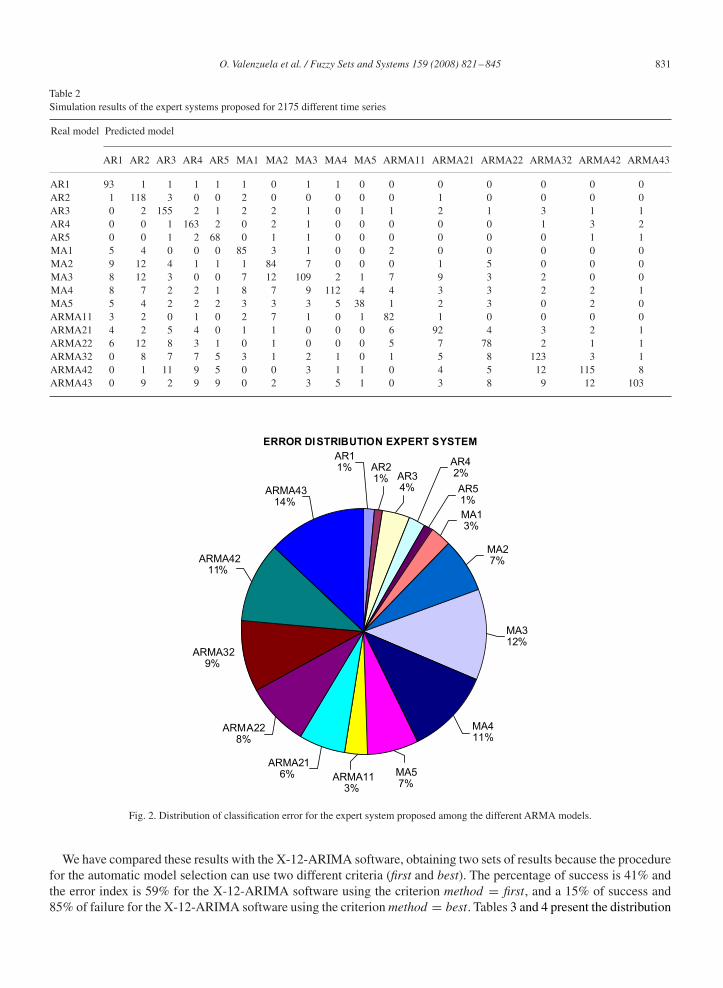
Table 2 shows the simulation results of the expert systems proposed for the 2175 different time series using AR,MA and ARMA models similar to those presented in [26]. In [26], a simple MLP, with two layers and conventionalnonlinear transfer functions, using the backpropagation algorithm for optimizing the connection of the neural network,produced some favourable results when compared with MLBP networks and the Box–Jenkins modelling approach fortime series forecasting, using ARMA(2,2) as the most complex model. In our case we have extended the models toARMA(4,3). From the global set of 2175 time series used for simulation, a total of 1618 were classified correctly;therefore the percentage of success is 74% and the error index is 26%. Fig. 2 shows graphically the error distributionfor the several ARMA models used.

O. Valenzuela et al. / Fuzzy Sets and Systems 159 (2008) 821–845 831

Table 2Simulation results of the expert systems proposed for 2175 different time series

Real model Predicted model

AR1 AR2 AR3 AR4 AR5 MA1 MA2 MA3 MA4 MA5 ARMA11 ARMA21 ARMA22 ARMA32 ARMA42 ARMA43

AR1 93 1 1 1 1 1 0 1 1 0 0 0 0 0 0 0AR2 1 118 3 0 0 2 0 0 0 0 0 1 0 0 0 0AR3 0 2 155 2 1 2 2 1 0 1 1 2 1 3 1 1AR4 0 0 1 163 2 0 2 1 0 0 0 0 0 1 3 2AR5 0 0 1 2 68 0 1 1 0 0 0 0 0 0 1 1MA1 5 4 0 0 0 85 3 1 0 0 2 0 0 0 0 0MA2 9 12 4 1 1 1 84 7 0 0 0 1 5 0 0 0MA3 8 12 3 0 0 7 12 109 2 1 7 9 3 2 0 0MA4 8 7 2 2 1 8 7 9 112 4 4 3 3 2 2 1MA5 5 4 2 2 2 3 3 3 5 38 1 2 3 0 2 0ARMA11 3 2 0 1 0 2 7 1 0 1 82 1 0 0 0 0ARMA21 4 2 5 4 0 1 1 0 0 0 6 92 4 3 2 1ARMA22 6 12 8 3 1 0 1 0 0 0 5 7 78 2 1 1ARMA32 0 8 7 7 5 3 1 2 1 0 1 5 8 123 3 1ARMA42 0 1 11 9 5 0 0 3 1 1 0 4 5 12 115 8ARMA43 0 9 2 9 9 0 2 3 5 1 0 3 8 9 12 103

ERROR DISTRIBUTION EXPERT SYSTEM

ARMA4314%

ARMA4211%

ARMA329%

ARMA228%

ARMA216% ARMA11

3%

MA57%

MA411%

MA312%

MA27%

MA13%

AR51%

AR34%

AR21%

AR11%

AR42%

Fig. 2. Distribution of classification error for the expert system proposed among the different ARMA models.

We have compared these results with the X-12-ARIMA software, obtaining two sets of results because the procedurefor the automatic model selection can use two different criteria (first and best). The percentage of success is 41% andthe error index is 59% for the X-12-ARIMA software using the criterion method = first, and a 15% of success and85% of failure for the X-12-ARIMA software using the criterion method = best. Tables 3 and 4 present the distribution

832 O. Valenzuela et al. / Fuzzy Sets and Systems 159 (2008) 821–845

Table 3Simulation results of the X-12-ARIMA software for 2175 different time series (automdl, method=first)

Real model Predicted model

AR1 AR2 AR3 AR4 AR5 MA1 MA2 MA3 MA4 MA5 ARMA11 ARMA21 ARMA22 ARMA32 ARMA42 ARMA43

AR1 83 1 1 1 1 1 2 1 1 0 0 2 0 0 0 0AR2 0 102 3 2 2 0 0 0 0 0 0 1 0 1 2 0AR3 0 2 141 2 0 5 5 0 1 1 1 6 0 0 1 0AR4 0 0 0 159 0 0 0 0 0 0 0 0 1 1 0 0AR5 0 0 0 0 66 0 1 0 0 2 0 0 1 0 0 0MA1 24 2 0 0 0 59 3 0 0 0 1 0 0 1 1 5MA2 1 57 4 1 1 0 46 0 0 0 2 1 0 0 0 3MA3 15 37 56 0 0 2 22 12 0 0 20 3 1 0 0 0MA4 34 13 11 26 1 10 8 4 48 0 0 1 2 2 2 3MA5 37 7 2 3 5 0 1 2 3 1 1 2 6 0 2 0ARMA11 0 0 0 0 0 0 30 1 0 1 62 1 0 0 0 0ARMA21 5 5 13 1 0 0 2 0 0 0 3 81 0 0 0 2ARMA22 1 33 15 20 2 0 0 0 0 0 9 22 4 2 1 1ARMA32 0 9 81 7 14 1 4 7 4 0 0 16 1 4 0 0ARMA42 0 3 27 92 4 0 0 0 1 1 0 9 3 1 22 3ARMA43 0 9 2 5 27 0 0 0 11 1 0 11 24 31 37 5

Table 4Simulation results of the X-12-ARIMA software for 2175 different time series (automdl, method=best)

Real model Predicted model

AR1 AR2 AR3 AR4 AR5 MA1 MA2 MA3 MA4 MA5 ARMA11 ARMA21 ARMA22 ARMA32 ARMA42 ARMA43

AR1 11 1 0 4 7 2 2 4 0 6 1 5 1 6 13 24AR2 0 11 6 7 17 0 0 0 0 0 0 2 4 11 28 27AR3 0 0 26 15 5 0 0 0 5 10 0 10 17 9 15 44AR4 0 0 0 31 16 0 0 0 1 5 0 0 8 16 36 43AR5 0 0 0 0 58 0 0 0 0 1 0 0 0 1 0 10MA1 4 5 2 9 11 3 2 1 0 2 0 0 3 2 13 41MA2 1 9 11 7 13 0 9 3 1 9 5 2 2 4 10 32MA3 1 0 17 5 12 2 9 11 1 5 3 10 15 4 22 52MA4 2 2 4 12 12 2 5 6 13 17 0 5 13 17 19 31MA5 0 0 2 1 19 0 0 2 2 6 0 1 6 12 8 16ARMA11 0 0 0 6 11 0 4 3 10 6 13 6 11 5 5 8ARMA21 0 0 3 4 11 0 0 0 0 2 2 17 15 10 17 26ARMA22 0 4 11 17 15 0 0 0 0 0 7 11 9 6 11 21ARMA32 0 2 14 25 25 1 0 1 5 8 0 5 10 13 10 35ARMA42 0 1 6 38 12 0 0 0 0 0 0 8 11 12 35 39ARMA43 0 1 0 0 19 0 0 0 0 0 0 3 7 21 43 73

of the error among the different ARMA models presented for both methods. Figs. 3 and 4 show graphically the errordistribution for the several ARMA models used in both simulations.

Other methods using soft-computing techniques have also been presented in the literature to effectively and easilyidentify the order of ARMA time series [20,39]. For example, in [13] an evolutionary algorithm searches for thebest ARMA model using only 8 time series, and therefore it is difficult to compare with the proposed expert system,also because in this paper no error index for model ARMA selection is obtained. Similar conclusions can be obtainedanalysing [41], where 4 time series are used for comparison. Also using evolutionary algorithms, in [53] a new approachto parameter estimation was presented. Although the practical work carried out in [53] was still in the beginning aspointed out by the authors, in order to analyse the behaviour of their algorithm, synthetic ARMA(3,3) were used for

O. Valenzuela et al. / Fuzzy Sets and Systems 159 (2008) 821–845 833

ERROR DISTRIBUTION X-12-ARIMA SOFTWARE

MA26%

MA13%

AR51%

AR41%

AR33%

AR22%

AR11%

ARMA4313%

ARMA4212%

ARMA3213%

ARMA229% ARMA21

3%ARMA11

3%

MA56%

MA410%

MA314%

Fig. 3. Distribution of classification error for X-12-ARIMA software (automdl, method = first) among the different ARMA models.

ERROR DISTRIBUTION X-12-ARIMA (USING BEST METHOD IN AUTOMDL)

AR51%

MA15%

ARMA329%

ARMA226%

ARMA216%

ARMA115%

MA54%

MA49%

MA38%

MA26%

AR48%

AR38%

AR26%

AR15%ARMA43

6%ARMA42

8%

Fig. 4. Distribution of classification error for X-12-ARIMA software (automdl, method = best) among the different ARMA models.

their study, and as an average index over all tested time series they concluded that a quota of about 20% of the modelswere correctly identified, taking into account the computation cost for each simulation.

It is important to note that not only the error index of the expert system presented in this paper is of relevance, butalso the computation time and the computational cost to select a specific ARMA model is very small, compared withsoft-computing techniques that use evolutionary algorithms or neural networks.

834 O. Valenzuela et al. / Fuzzy Sets and Systems 159 (2008) 821–845

10 11 12 13 14 15 16 17 18 19 200

10

20

30

40

50

60

SIGNAL

HIS

TO

GR

AM

10 11 12 13 14 15 16 17 18 19 20-1.5

-1

-0.5

0

0.5

1

1.5

2

2.5

3

3.5

PHASE PORTRAITS

X

Δ X

Fig. 5. The characterization of the Eriel time series: (a) histogram and (b) the phase diagram.

4.2. Analysis of the complete hybrid system

Once the forecasting methodology has been established, we can proceed with our intensive experimental studies.In this section, we provide several numerical examples to evaluate the advantages and the effectiveness of the pro-posed approach. We have used the root mean squared error (RMSE) and the correlation coefficient as performancemeasures.The expression for the RMSE is

RMSE =√√√√1

n

n∑t=1

(yt − yt )2. (13)

A. Monthly lake Erie levels: A very interesting problem is the prediction of data that are not generated from a math-ematical expression and thus governed by a particular determinism. For this purpose, we used a natural phenomenon,the monthly lake Erie levels from 1921 to 1970. The first 400 data pairs of the series were used as training data, whilethe remaining 200 where used to validate the model identified. Fig. 5 shows a characterization of this time series(its histogram and its phase diagram). Fig. 6 shows the predicted and desired values (dashed and continuous lines,respectively) using only ANNs and Fig. 7 shows the forecasting using the hybrid method. The error indices (RMSEand correlation coefficient) for both simulations are, respectively, [0.1045, 0.937] and [0.0820, 0.963]. Finally, Fig. 8shows the results of correlating one prediction step ahead.

B. Sunspots: This time series is a real series of the yearly sunspot data from 1770 to 1869. This series also has beenanalysed by Box and Jenkins, and is identified as having an ARMA(2,0) model or ARMA(2,1) model [43]. Fig. 9 showsthis time series. The error index RMSE is [16.71, 9.32, 7.25] for the ARMA(2,1) model, using only ANNs and usingthe hybrid method, respectively.

C. Stocks of evaporated and sweetened condensed milk: This series is taken from Makridakis et al. [37], and has atotal of 120 data. The expert system proposed in this paper selects and ARMA(3,2) for this time series. Fig. 10 showsthis time series. The error index RMSE is [12.06, 7.54, 5.86] for the ARMA(3,2) model, using only ANNs and usingthe hybrid method, respectively.

D. Australian Monthly electricity production data from January 1980 to August 1995: This series is also taken from[37], and has a total of 476 data. The expert system proposed in this paper selects an ARMA(3,2) for this time series.Fig. 11 shows this time series. The error index RMSE is [411.271, 232.23, 193.21] for the ARMA(3,2) model, usingonly ANNs and using the hybrid method, respectively.

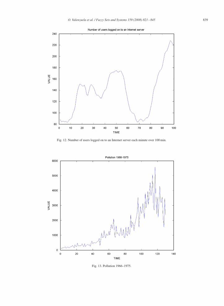
E. Number of users logged on to an Internet server each minute over 100 min: This series is also taken from [37],and has a total of 100 data. The expert system proposed in this paper selects an ARMA(4,3) for this time series. Fig. 12shows this time series. The error index RMSE is [3.01, 2.41, 1.95] for the ARMA(4,3) model, using only ANNs andusing the hybrid method, respectively.

O. Valenzuela et al. / Fuzzy Sets and Systems 159 (2008) 821–845 835

0 50 100 150 200 250 300 350 400 450 500-1

-0.8

-0.6

-0.4

-0.2

0

0.2

0.4

0.6

0.8

1

DESIRED (SOLID LINE) AND PREDICTED (DASHED LINE)

0 100 200 300 400 500 600-0.4

-0.3

-0.2

-0.1

0

0.1

0.2

0.3

0.4

0.5PREDICTION ERRORS

a

b

Fig. 6. Eriel time series (prediction step=1): (a) result of the original and predicted Eriel time series using only ANN and (b) prediction error.

F. Pollution 1966–1975: This series is also taken from [37], has a total of 130 data and represents the monthlyshipment of pollution equipment from January 1966 through December 1975 (in thousands of French francs). Theexpert system proposed in this paper selects an ARMA(4,3) for this time series. Fig. 13 shows this time series. Theerror index RMSE is [371.5, 213.8, 197.4] for the ARMA(4,3) model, using only ANNs and using the hybrid method,respectively.

G. Mackey–Glass chaotic time series: The methodology proposed in this paper has also been tested with thetime series generated by the Mackey–Glass time-delay differential equation (a very well-known benchmarkproblem [67]).

dx(t)

dt= ax(t − )

1 + x10(t − )− bx(t). (14)

836 O. Valenzuela et al. / Fuzzy Sets and Systems 159 (2008) 821–845

0 50 100 150 200 250 300 350 400 450-1

-0.5

0

0.5

1

1.5

DESIRED (SOLID LINE) AND PREDICTED (DASHED LINE). HYBRID SYSTEM

0 50 100 150 200 250 300 350 400 450-0.4

-0.3

-0.2

-0.1

0

0.1

0.2

0.3

0.4PREDICTION ERRORS

a

b

Fig. 7. Eriel time series (prediction step=1): (a) result of the original and predicted Eriel time series using proposed methodology (which areindistinguishable) and (b) prediction error.

Following the previous studies [30,32], the parameters were fixed to a = 0.2 and b = 0.1. One thousand data pointswere generated with an initial condition x(0) = 1.2, thus obtaining a chaotic time series with no clearly defined period;it does not converge or diverge, and is very sensitive to the initial conditions. The time series values at integer pointswere obtained applying the fourth-order Runge–Kutta method to find the numerical solution for the above equation.The values = 17 and x(t) = 0 for t < 0 were assumed. This data set can be found in the file mgdata.dat belongingto the Fuzzy logic Toolbox of Matlab.

Fig. 14 shows a section of 1000 sample points used in our study. The first 500 data pairs of the series were used astraining data, while the remaining 500 were used to validate the model identified. We compare again the behaviour of

O. Valenzuela et al. / Fuzzy Sets and Systems 159 (2008) 821–845 837

-1 -0.8 -0.6 -0.4 -0.2 0 0.2 0.4 0.6 0.8 1-1

-0.5

0

0.5

1

1.5

ORIGINAL DATA

PR

ED

ICT

ED

DA

TA

Fig. 8. Correlation for the Eriel time series using the proposed methodology.

Fig. 9. Sunspot time series.

the forecasting result using the proposed hybrid methodology and only ANNs. The error indices, the root mean squareerror and the correlation coefficient, for this simulation were 0.0122 and 0.998 for the model using only ANNs and0.0027 and 1 for the proposed algorithm. Fig. 14a shows the forecasting using the hybrid methodology.

838 O. Valenzuela et al. / Fuzzy Sets and Systems 159 (2008) 821–845

Fig. 10. Stocks of evaporated and sweetened condensed milk time series.

Fig. 11. Australian monthly electricity production data from January 1980 to August 1995.

O. Valenzuela et al. / Fuzzy Sets and Systems 159 (2008) 821–845 839

Fig. 12. Number of users logged on to an Internet server each minute over 100 min.

Fig. 13. Pollution 1966–1975.

840 O. Valenzuela et al. / Fuzzy Sets and Systems 159 (2008) 821–845

0 100 200 300 400 500 600 700 800-1

-0.5

0

0.5

1

1.5

DESIRED (SOLID LINE) AND PREDICTED

(DASHED LINE). HYBRID SYSTEM

0 100 200 300 400 500 600 700 800-0.01

-0.008

-0.006

-0.004

-0.002

0

0.002

0.004

0.006

0.008

0.01PREDICTION ERRORS

-1 -0.8 -0.6 -0.4 -0.2 0 0.2 0.4 0.6 0.8 1

-1

-0.5

0

0.5

1

1.5

ORIGINAL DATA

PR

ED

ICT

ED

DA

TA

a

b

c

Fig. 14. Mackey–Glass time series (prediction step=6): (a) result of the original and predicted Mackey–Glass time series using proposed methodology,(b) prediction error and (c) correlation for the time series using the proposed hybrid methodology.

O. Valenzuela et al. / Fuzzy Sets and Systems 159 (2008) 821–845 841

Table 5Comparison results of the prediction error of different methods for prediction step equals to 6 (500 training data)

Method Prediction error (RMSE)

Auto regressive model 0.19Cascade correlation NN 0.06Back-Prop. NN 0.02Sixth-order polynomial 0.04Linear predictive method 0.55Kim and Kim (genetic algorithm and fuzzy system)

5 MFs 0.0492067 MFs 0.0422759 MFs 0.037873

Jang et al. (ANFIS and fuzzy system) 0.007Wang et al.

Product T-norm 0.0907Min T-norm 0.0904

Classical neural network using RBF 0.0114Our approach 0.0027

Table 5 compares the prediction accuracy of different computational paradigms presented in the literature for thisbenchmark problem (including our proposal), for various fuzzy system structures, neural systems and genetic algo-rithms. The data are taken from [28,30,32].

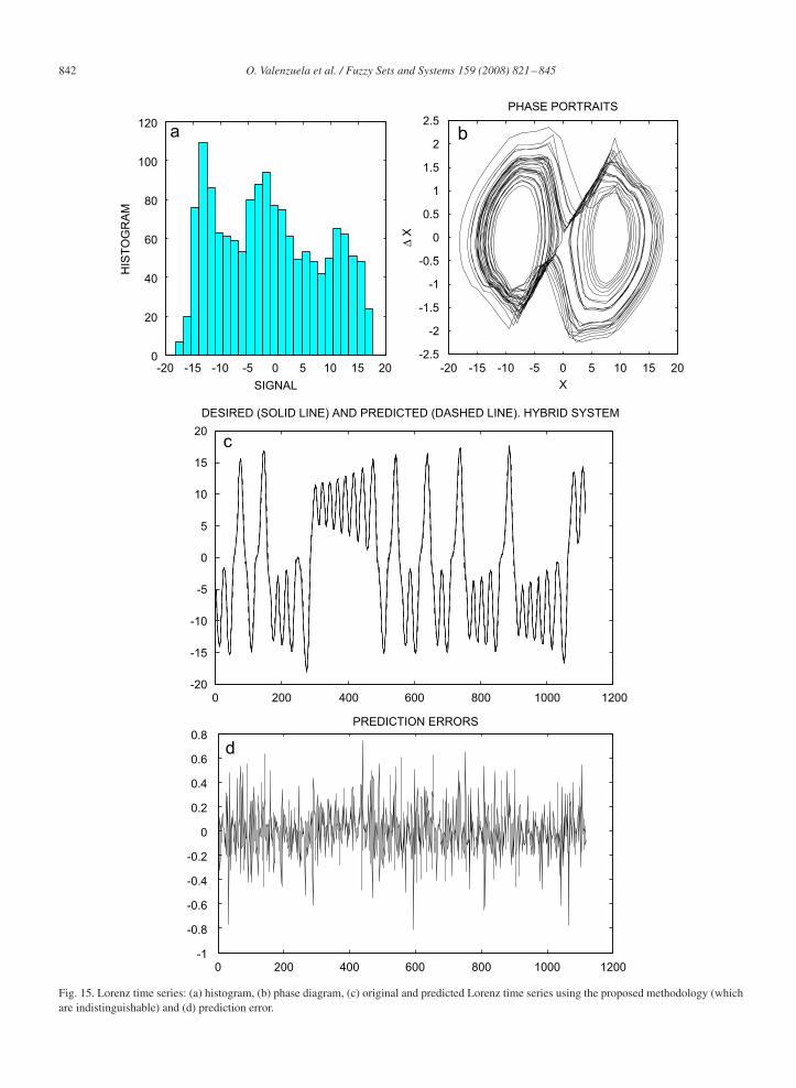
H. Lorenz attractor time series: The Lorenz equations were discovered by Ed Lorenz in 1963 as a very simplifiedmodel of convection rolls in the upper atmosphere. Later these same equations appeared in studies of lasers, batteries,and in a simple chaotic waterwheel that can be easily built. They have been used as a benchmark problem in time seriesprediction. The trajectories obtained when resolving this equations, for certain settings neither converge to a fixed pointor a fixed cycle, nor diverge to infinity. A long trajectory of the Lorenz attractor (1500 points) was generated using adifferential equation solver (Runge–Kutta method) with step size of 0.05 to create a univariate time series. The datawere split into two parts: 1127 points were used for training and the remaining 361 for assessing the generalizationcapability of the model.

Fig. 15a and b shows a characterization of this time series (its histogram and its phase diagram). Fig. 15c shows theprediction of the Lorenz attractor using the proposed methodology. As they are practically identical, the difference canonly be seen on a finer scale (Fig. 15d). The error indices, i.e. the root mean square error and the correlation coefficient,for this simulation were 0.176 and 0.998 for the model using only ANNs and 0.0876 and 0.9996 for the proposedalgorithm. It is important to note other approaches appeared in the literature; for example Iokibe et al. [27] obtain anRMSE of 0.244, Jang et al. [28] an RMSE of 0.143, using fuzzy and neuro-fuzzy systems. Fig. 16 shows the resultsof correlating one prediction step ahead. Finally, Fig. 17 shows the prediction result of the Lorenz attractor when theprediction step is modified.

5. Conclusion

In this work we have proposed a hybrid ARIMA–ANN model for time series prediction. This model synergi-cally combines the advantages of the easy-to-use and relatively easy-to-tune ARIMA models, and the computationalpower of ANNs. In order to obtain the order of differencing of the integrative part of the ARIMA model, and theorder of the underlying AR and MA parts, we have proposed the use of an expert fuzzy logic-based system whoserules are weighted in an automatic way, without the intervention of a human expert. To solve this last problem, wehave designed an evolutionary algorithm whose fitness function, stop condition and cross-over and mutation oper-ators have been specifically chosen. The simulations performed show that the synergy of the different paradigmsand techniques used produce excellent results for the construction of intelligent systems for automatic time seriesforecasting.

842 O. Valenzuela et al. / Fuzzy Sets and Systems 159 (2008) 821–845

-20 -15 -10 -5 0 5 10 15 200

20

40

60

80

100

120

SIGNAL

HIS

TO

GR

AM

-20 -15 -10 -5 0 5 10 15 20-2.5

-2

-1.5

-1

-0.5

0

0.5

1

1.5

2

2.5

PHASE PORTRAITS

X

Δ X

a b

0 200 400 600 800 1000 1200-20

-15

-10

-5

0

5

10

15

20

DESIRED (SOLID LINE) AND PREDICTED (DASHED LINE). HYBRID SYSTEM

0 200 400 600 800 1000 1200-1

-0.8

-0.6

-0.4

-0.2

0

0.2

0.4

0.6

0.8PREDICTION ERRORS

c

d

Fig. 15. Lorenz time series: (a) histogram, (b) phase diagram, (c) original and predicted Lorenz time series using the proposed methodology (whichare indistinguishable) and (d) prediction error.

O. Valenzuela et al. / Fuzzy Sets and Systems 159 (2008) 821–845 843

-20 -15 -10 -5 0 5 10 15 20-20

-15

-10

-5

0

5

10

15

20

ORIGINAL DATA

PR

ED

ICT

ED

DA

TA

Fig. 16. Correlation for the Lorenz time series using the proposed methodology.

1 2 3 4 5 6 7 8 9 100

0.5

1

1.5

2

2.5

LORENZ ATTRACTOR

PREDICTION STEP

RM

SE

Training

Test

Fig. 17. Prediction performance for the Lorenz attractor time series (change of RMSE by prediction step).

Acknowledgements

This work has been partially supported by the Spanish Projects TIN2004-01419 and TIN2007-60587. We also wantto thank the anonymous reviewers for their helpful and accurate comments.

844 O. Valenzuela et al. / Fuzzy Sets and Systems 159 (2008) 821–845

References

[1] T. Al-Saba, I. El-Amin, Artificial neural networks as applied to long-term demand forecasting, Artificial Intelligence Eng. 13 (1999) 189–197.[2] A.-S. Adnan, A. Ahmad, Fitting ARMA models to linear non-Gaussian processes using higher order statistics, Signal Process. 82 (2002)

1789–1793.[3] R. Azencott, Modelisation ARIMA automatique: le systeme MANDRAKE, Cahiers du Centre d ’Etudes de Recherche Operationnelle 32 (1990)

229.[4] M.A. Baxter, A guide to seasonal adjustment of monthly data with X-11, third ed., Central Statistical Office, UK, 1994.[5] J.M. Beguin, C. Gourieroux,A. Monfort, Identification of a mixed autoregressive-moving average process: the Corner method, in: O.D.Anderson

(Ed.), Time Series, North-Holland, Amsterdam, 1980.[6] G.E.P. Box, G.M. Jenkins, G.C. Reinsel, Time Series Analysis: Forecasting and Control, Prentice-Hall, Englewood Cliffs, NJ, 1994.[7] G.E.P. Box, D.A. Pierce, Distribution of residual autocorrelations in autoregressive integrated moving average time series models, J. Amer.

Statist. Assoc. 65 (1970) 1509–1526.[8] O. Castillo, P. Melin, Hybrid intelligent systems for time series prediction using neural networks, fuzzy logic, and fractal theory, IEEE Trans.

Neural Networks 13 (6) (2002).[9] P.A. Castillo-Valdivieso, J.J. Merelo, A. Prieto, I. Rojas, G. Romero, Statistical analysis of the parameters of a neuro-genetic algorithm, IEEE

Trans. Neural Networks 13 (6) (2002) 1374–1394.[10] W.-S. Chan, A comparison of some of pattern identification methods for order determination of mixed ARMA models, Statist. Probab. Lett. 42

(1999) 69–79.[11] S.-M. Chen, C.-M. Huang, Generating weighted fuzzy rules from relational database systems for estimating null using genetic algorithms,

IEEE Trans. Fuzzy Systems 11 (4) (2003).[12] W.S. Cleveland, S. Devlin, E. Grosse, Regression by local fitting: methods, properties and computational algorithms, J. Econometrics 37 (1988)

87–114.[13] P. Cortez, M. Rocha, Evolving time series forecasting ARMA models, J. Heuristics 10 (4) (2004) 415–429.[14] J.W. Denton, How good are neural networks for causal forecasting?, J. Business Forecasting 14 (1995) 17–20.[15] M.M. Elkateb, K. Solaiman, Y. Al-Turki, A comparative study of medium-weather-dependent load forecasting using enhanced artificial-fuzzy

neural network and statistical techniques, Neurocomputing 23 (1998) 3–13.[16] L.J. Eshelman, J.D. Shaffer, Real-Coded Genetic Algorithms and Interval-Schema, Foundation of Genetic Algorithms 2, Morgan Kaufmann,

Los Altos, CA, 1993 pp. 187–202.[17] T.-G. Fan, S.-T. Wang, J.-M. Chen, Generating weighted fuzzy production rules using neural networks, in: Proc. Fifth Internat. Conf. Machine

Learning and Cybernetics, Dalian, 13–16 August 2006.[18] D.F. Findley, B.C. Monsell, W.R. Bell, M.C. Otto, B.C. Chen, New capabilities and methods of the X-12-ARIMA seasonal adjustment program,

J. Business Econom. Statist. (1997).[19] E.J. Hannan, J. Rissanen, Recursive estimation of mixed autogressive-moving average order, Biometrika 69 (1) (1982) 81–94.[20] M. Haseyama, H. Kitajima, An ARMA order selection method with fuzzy reasoning, Signal Process. 81 (2001) 1331–1335.[21] L.J. Herrera, H. Pomares, I. Rojas, O. Valenzuela, M. Awad, MultiGrid-based fuzzy systems for function approximation, in: Advances in

Artificial Intelligence, in: Lecture Notes in Computer Science, Vol. 2972, 2004, pp. 252–261.[22] T. Hill, M. O’Connor, W. Remus, Neural network models for time series forecasts, Management Sci. 42 (7) (1996) 1082–1092.[23] Y. Huang, C. Haung, Real-valued genetic algorithms for fuzzy grey prediction system, Fuzzy Sets and Systems 87 (1997) 265–276.[24] C.M. Hurvich, C.-L. Tsai, Regression and time series model selection in small samples, Biometrica 76 (2) (1989) 297–307.[25] H.B. Hwang, Insights into neural-network forecasting time series corresponding to ARMA(p; q) structures, Omega 29 (2001) 273–289.[26] H.B. Hwang, H.T. Ang, A simple neural network for ARMA(p; q) time series, Omega 29 (2001) 319–333.[27] T. Iokibe, Y. Fujimoto, M. Kanke, S. Suzuki, Short-term prediction of chaotic time series by local fuzzy reconstruction method, J. Intelligent

Fuzzy Systems 5 (1997) 3–21.[28] J.S.R. Jang, C.T. Sun, E. Mizutani, Neuro-Fuzzy and Soft Computing, Prentice-Hall, Englewood Cliffs, NJ, 1997, 0-13-261066-3.[29] R.H. Jones, Fitting autoregressions, J. Amer. Statist. Assoc. 70 (351) (1975) 590–592.[30] D. Kim, C. Kim, Forecasting time series with genetic fuzzy predictor ensemble, IEEE Trans. Fuzzy Systems 5 (4) (1997) 523–535.[31] T. Koutroumanidis, L. Iliadis, G.K. Sylaios, Time-series modeling of fishery landings using ARIMA models and fuzzy expected intervals

software, Environmental Modelling Software 21 (12) (2006) 1711–1721.[32] S.-H. Lee, I. Kim, Time series analysis using fuzzy learning, in: Proc. Internat. Conf. on Neural Information Processing, Seoul, Korea, Vol. 6,

October 1994, pp. 1577–1582.[33] J. Liska, S.S. Melsheimer, Complete design of fuzzy logic systems using genetic algorithm, in: Proc. of FUZZ-IEEE’94, 1994, pp. 1377–1382.[34] G.M. Ljung, G.E.P. Box, On a measure of lack of fit in time series models, Biometrika 65 (1978) 297–307.[35] L. Ljung, System Identification Theory for the User, Prentice-Hall, Englewood Cliffs, NJ, 1987.[36] S. Makridakis, A. Anderson, R. Carbone, R. Fildes, M. Hibon, R. Lewandowski, J. Newton, E. Parzen, R. Winker, The Forecasting Accuracy

of Major Time Series Methods, Wiley, New York, 1984.[37] S. Makridakis, S. Wheelwright, R. Hyndman, Forecasting: Methods and Applications, third ed., Wiley, New York, 1998

〈http://www-personal.buseco.monash.edu.au/∼hyndman/forecasting/gotodata.htm〉.[38] Z. Michalewicz, Genetic Algorithms + Data Structures = Evolution Programs, Springer, Berlin, 1996.[39] T. Minerva, I. Poli, Building ARMA models with genetic algorithms, in: Lecture Notes in Computer Science, Vol. 2037, 2001, pp. 335–342.[40] D. Nauck, R. Kruse, How the learning of rule weights affects the interpretability of fuzzy systems, in: Proc. 7th IEEE Internat. Conf. on Fuzzy

Systems, Anchorage, May 4–9, 1998, pp. 1235–1240.

O. Valenzuela et al. / Fuzzy Sets and Systems 159 (2008) 821–845 845

[41] C.-S. Ong, J.-J. Huang, G.-H. Tzeng, Model identification of ARIMA family using genetic algorithms, Appl. Math. Comput. 164 (3) (2005)885–912.

[42] P.-F. Pai, C.-S. Lin, A hybrid ARIMA and support vector machines model in stock price forecasting, Omega 33 (6) (2005) 497–505.[43] Y.R. Park, T.J. Murray, C. Chen, Predicting sun spots using a layered perceptron neural network, IEEE Trans. Neural Networks 7 (2) (1996)

501–505.[44] H. Pomares, I. Rojas, J. Gonzalez, A. Prieto, Structure identification in complete rule-based fuzzy systems, IEEE Trans. Fuzzy Systems 10 (3)

(2002) 349–359.[45] H. Pomares, I. Rojas, J. Ortega, J. Gonzalez, A. Prieto, A systematic approach to a self-generating fuzzy rule-table for function approximation,

IEEE Trans. Systems Man Cybernet. B 30 (3) (2000) 431–447.[46] I. Rojas, H. Pomares, J. Ortega, A. Prieto, Self-organized fuzzy system generation from training examples, IEEE Trans. Fuzzy Systems 8 (1)

(2000) 23–36.[47] I. Rojas, H. Pomares, J.L. Bernier, J. Ortega, B. Pino, F.J. Pelayo, A. Prieto, Time series analysis using normalized PG-RBF network with

regression weights, Neurocomputing 42 (1–4) (2002) 267–285.[48] I. Rojas, H. Pomares, J. Gonzales, et al., Analysis of the functional block involved in the design of radial basis function networks, Neural

Process. Lett. 12 (1) (2000) 1–17.[49] I. Rojas, J. Ortega, F.J. Pelayo, A. Prieto, Statistical analysis of the main parameters in the fuzzy inference process, Fuzzy Sets and Systems

102 (2) (1999).[50] I. Rojas, O. Valenzuela, M. Anguita, A. Prieto, Analysis of the operators involved in the definition of the implication functions and in the fuzzy

inference process, Internat. J. Approx. Reason. 19 (3–4) (1998) 367–389.[51] I. Rojas, F. Rojas, H. Pomares, L.J. Herrera, J. Gonzalez, O. Valenzuela, The synergy between classical and soft-computing techniques for time

series prediction, in: Advances in Artificial Intelligence, Lecture Notes in Computer Science, Vol. 2972, 2004, pp. 30–39.[52] I. Rojas, H. Pomares, J. Ortega, A. Prieto, Self-organized fuzzy system generation from training examples, IEEE Transactions on Fuzzy Systems

8 (1) (2000) 23–36.[53] S. Rolf, J. Sprave, W. Urfer, Model identification and parameter estimation of ARMA models by means of evolutionary algorithms, in: Proc.

of IEEE/IAFE 1997 Computational Intelligence for Financial Engineering (CIFEr), 1997, pp. 237–243.[54] T.L. Seng, M.B. Khalid, R. Yusof, Tuning of a neuro-fuzzy controller by genetic algorithm, IEEE Trans. Systems Man Cybernet. B 29 (2)

(1999) 226–235.[55] R. Shibata, Selection of the order of an autoregressive model by Akaike’s information criterion, Biometrika AC-63 (1) (1976) 117–126.[56] R.C. Souza, A.C. Neto, A bootstrap simulation study in ARMA(p, q) structures, J. Forecasting 15 (1996) 343–353.[57] Z. Tang, C. Almeida, P.A. Fishwick, Time series forecasting using neural networks vs. Box–Jenkins methodology, Simulation 57 (5) (1991)

303–310.[58] Z. Tang, P.A. Fishwick, Back-propagation neural nets as models for time series forecasting, ORSA J. Comput. 5 (4) (1993) 374–385.[59] L.J. Tashman, Out-of sample tests of forecasting accuracy: a tutorial and review, Internat. J. Forecasting 16 (2000) 437–450.[60] M. Teng, F. Xiong, R. Wang, Z. Wu, Using genetic algorithm for weighted fuzzy rule-based system, Intelligent Control Automat. (2004)

4292–4295.[61] R.S. Tsay, G.C. Tiao, Consistent estimates of autoregressive parameters and extended sample autocorrelation function for stationary and

nonstationary ARMA model, J. Amer. Statist. Assoc. 79 (1) (1984) 84–96.[62] R.S. Tsay, G.C. Tiao, Use of canonical analysis in time series model identification, Biometrika 72 (2) (1985) 299–315.[63] F.M. Tseng, H. Yu, G. Tzeng, Combining neural network model with seasonal time series ARMA model, Technological Forecasting Social

Change 69 (2002) 71–87.[64] L.X. Wang, J.M. Mendel, Generating fuzzy rules by learning from examples, IEEE Trans. Systems Man Cybernet. 22 (6) (1992) 1414–1427.[65] D.K. Wedding II, K.J. Cios, Time series forecasting by combining RBF networks, certainty factors, and the Box–Jenkins model, Neurocomputing

10 (1996) 149–168.[66] A.S. Weigend, N.A. Gershenfeld, Time Series Prediction, Addison-Wesley, Reading, MA, 1994.[67] B.A. Whitehead, T.D. Choate, Cooperative-competitive genetic evolution of radial basis function centers and widths for time series prediction,

IEEE Trans. Neural Networks 7 (4) (1996) 869–880.[68] W.A. Woodward, H.L. Gray, On the relationship between the S array and the Box–Jenkins method of ARMA model identification, J. Amer.

Statist. Assoc. 76 (3) (1981) 579–587.[69] A. Wright, Genetic Algorithms for Real Parameter Optimization, Foundation of Genetic Algorithms, Morgan Kaufmann Publishers, Los Altos,

CA, 1991 pp. 205–218.[70] 〈http://www-personal.buseco.monash.edu.au/∼hyndman/TSDL/physics.html/〉.[71] 〈http://www.omatrix.com/stsa.html/〉 (STSA toolbox).[72] 〈http://www.census.gov/srd/www/x12a/〉 (X-12-ARIMA software).[73] J. Yao, H.L. Poh, Forecasting the KLSE index using neural networks, in: Internat. Conf. on Neural Networks, Vol. 2, 1995, pp. 1012–1017.[74] G.P. Zhang, Time series forecasting using a hybrid ARMA and neural network model, Neurocomputing 50 (2003) 159–175.