Vol. 43, No. 1, February 2009, pp. 27–42issn 0041-1655 �eissn 1526-5447 �09 �4301 �0027

informs ®

doi 10.1287/trsc.1080.0251©2009 INFORMS

Hybrid Adaptive Predictive Control for a DynamicPickup and Delivery Problem

Cristián E. CortésCivil Engineering Department, Universidad de Chile, Avenue Blanco Encalada 2002,

Santiago, Chile, ccortes@ing.uchile.cl

Doris Sáez, Alfredo Núñez, Diego Muñoz-CarpinteroElectrical Engineering Department, Universidad de Chile, Avenue Tupper 2007, Santiago, Chile

{dsaez@ing.uchile.cl, alfnunez@ing.uchile.cl, dimunoz@ing.uchile.cl}

This paper presents a hybrid adaptive predictive control approach that includes future information in real-time routing decisions in the context of a dynamic pickup and delivery problem (DPDP). We recognize in

this research that when the problem is dynamic, an additional stochastic effect has to be considered withinthe analytical expression of the objective function for vehicle scheduling and routing, which is the extra costassociated with potential rerouting arising from unknown requests in the future. The major contributions of thispaper are: first, the development of a formal adaptive predictive control framework to model the DPDP, andsecond, the development and coding of an ad hoc particle swarm optimization (PSO) algorithm to efficientlysolve it. Predictive state-space formulations are written on the relevant variables (vehicle load and departuretime at stops) for the DPDP. Next, an objective function is stated to solve the real-time system when predictingone and two steps ahead in time. A problem-specific PSO algorithm is proposed and coded according to thedynamic formulation. Then, the PSO method is used to validate this approach through a simulated numericalexample.

Key words : pickup-and-delivery system; dynamic vehicle routing problem; hybrid predictive control; particleswarm optimization

History : Received: March 2005; revisions received: April 2006, July 2007, October 2007; accepted: October 2008.

1. IntroductionOne of the most studied problems in the literatureon logistics is the well-known pickup and deliv-ery problem (with or without time windows), whichinvolves the satisfaction of a set of transportationrequests by a vehicle fleet initially located at sev-eral depots (Desrosiers, Soumis, and Dumas 1986;Savelsbergh and Sol 1995). A transportation requestconsists of picking up a certain number of customersat a predetermined pickup location during a depar-ture time interval and taking them to a predetermineddelivery location within an arrival time interval. Load-ing and unloading times are incurred at each vehiclestop. The problem can be generalized to the dynamiccase, in which a subset of the requests is not knownin advance and dispatch decisions have to be madein real time. The dynamic pickup and delivery prob-lem (DPDP) has become of great interest in the lastdecade, mainly due to the fast growth in communi-cation and information technologies, as well as thecurrent interest in real-time dispatching and routing.The problem can be characterized as a real-time routedtransit and has been treated mostly heuristically bymany authors under different policy schemes in thepast (as representative references see Psaraftis 1988;Madsen, Raven, and Rygaard 1995; Bertsimas and

Van Ryzin 1991, 1993a, b; Malandraki and Daskin 1992;Dial 1995; Gendreau et al. 1999).In this scenario, if the objective were to transport

passengers, inefficient routing decisions could greatlyaffect the performance of the system as perceived bythe users, resulting in a poor level of service, lowdemand, and insufficient productivity. One of themajor issues for improving efficiency is the correct def-inition of a decision objective function for dispatch-ing, including total travel and waiting times for usersas well as a performance measure for vehicles. How-ever, when the problem is dynamic, an additionalstochastic effect has to be considered when comput-ing an analytical expression for any decision objectivefunction (whether it affects the user or the operator).In other words, we recognize that current dispatchactions taken in real time can be affected by poten-tial rerouting decisions decided in the future, affectingmost customers already in the system, those waiting,as well as those traveling.The importance of this issue has been underesti-

mated in the dynamic vehicle-routing literature. Oneassumption behind most of the proposed schedul-ing-routing rules is that travel and waiting timesexperienced by customers are considered fixed in theobjective function expressions, independent of future

27

Cortés et al.: Hybrid Adaptive Predictive Control for a Dynamic Pickup and Delivery Problem28 Transportation Science 43(1), pp. 27–42, © 2009 INFORMS

reroutings. In other words, as stated by Spivey andPowell (2004), the complexity of real-time routingschemes have generally restricted research to myopicmodels (for example, see Wilson and Weissberg 1976;Wilson and Colvin 1977; Psaraftis 1980, 1988; Madsen,Raven, and Rygaard 1995; Gendreau et al. 1999;Swihart and Papastavrou 1999).However, some recent studies in the field of vehicle

routing and dispatching have tried to exploit infor-mation about future events to improve decision mak-ing (Ichoua, Gendreau, and Potvin 2006; Spivey andPowell 2004). Solution approaches found in this lineof research are diverse, with formulations based upondynamic network models (Powell 1988), dynamicand stochastic programming schemes (Godfrey andPowell 2002, Topaloglu and Powell 2005), etc. Cortésand Jayakrishnan (2004) propose a scheme for makingbetter dynamic decisions by estimating the effectivecost of a real-time request insertion based upon futureinformation. The authors realized that the problemconceptually fits within a stochastic predictive controlframework, although they did not enter into the con-trol formulation details.In this paper, we formalize the approach suggested

by Cortés and Jayakrishnan (2004) by developing aconsistent framework based upon predictive controltheory for optimizing the performance of a DPDPthat is mainly oriented to passenger movements. Theformulation turned out to be highly nonlinear, with acombination of integer/discrete and continuous vari-ables to properly describe the future behavior of therouting process. Hence, an efficient ad hoc algorithmfrom the computational intelligence literature (parti-cle swarm optimization, PSO) is developed to solvethe proposed formulation and to test the benefits ofincorporating demand patterns’ prediction in currentrouting decisions under different scenarios.Unlike others’ nonmyopic dynamic vehicle-routing

approaches, this formulation is based on state-spacevariables. The system state is defined in terms ofdeparture time and vehicle loads (stochastic state-space variables), the system inputs (control actions)are routing decisions, the system outputs are effec-tive departure time to stops, and the demand requestsare modeled as disturbances. We use a discrete modelwith variable step size equal to the time between suc-cessive calls (events). In order to include future andunknown demand in the current decision, we solvean objective function incorporating the predictiveeffect via probabilities computed from historical dataregarding typical demand patterns.In summary, we highlight two major contributions

of this paper: the development of a hybrid predictivecontrol framework to model the DPDP, and the devel-opment of an ad hoc PSO algorithm to efficiently solvethe proposed formulation for real-size problems. This

line of research represents an innovative attempt todevelop control-based algorithms for modeling andsolving dynamic transportation problems in a realis-tic context. Specifically, in this application we havedeveloped a new version of the PSO algorithm (orig-inally conceived for solving continuous problems) inorder to add integer variables into the solution andsolve the DPDP efficiently. It is important to mentionthat the proposed algorithm was conceived from thehybrid predictive control scheme (HPC) to deal withthe DPDP developed here, and depends exclusivelyon the structure of the HPC formulation, as shownin §3.4.The structure of the paper is as follows. In the next

section, the relevant background on dynamic vehi-cle routing is presented. In §3, the dynamic pickupand delivery problem is described in context, andis formulated under an adaptive-predictive controlscheme. Thus, the specific state-space formulation forthe problem is developed, the associated dispatchobjective function is shown, and the solution algo-rithms are developed to solve the proposed hybridpredictive control scheme. In §4, a numerical exampleis presented to show the benefits of applying predic-tive control at least two steps ahead in time. Finally,in §5, analysis, comments, and further research linesare presented.

2. The Dynamic Vehicle-RoutingProblem: Approaches andSolution Methods

In this section, the objective is to provide a reviewon the most relevant dynamic vehicle-routing prob-lem (DVRP) variants, intensely studied by differentauthors with different applications over the past 15to 20 years. DVRPs are characterized by routes thatare constructed as unknown requests enter the systemin real time. Thus, DVRPs are formulated by assum-ing that inputs may change or have to be updatedduring the execution of the solution algorithm. Larsen(2000) develops a nice characterization of the dif-ferent dynamic problems, starting again from theTSP (traveling salesman problem), which yields thedynamic TSP (DTSP) introduced by Psaraftis (1988).This work motivates the development of the dynamictraveling repairman problem (DTRP), introduced byBertsimas and Van Ryzin (1991) and next extended byBertsimas and Van Ryzin (1993a, b). Lately, Swihartand Papastavrou (1999), and Thomas andWhite (2004)formulate and solve two variants of the DTRP.The dynamic pickup and delivery problem (DPDP)

that is designed to solve the dynamic dial-a-rideProblem (DDRP) has been intensely studied in thelast 20 years (Psaraftis 1980, 1988; Gendreau et al.1999; Savelsbergh and Sol 1995). The final output of

Cortés et al.: Hybrid Adaptive Predictive Control for a Dynamic Pickup and Delivery ProblemTransportation Science 43(1), pp. 27–42, © 2009 INFORMS 29

such a problem is a set of routes for all vehicles,which dynamically change over time. With regard toreal applications, Madsen, Raven, and Rygaard (1995)adapt the insertion heuristics by Jaw et al. (1986) andsolve a real-life problem for moving elderly and hand-icapped people in Copenhagen, whereas Dial (1995)proposes a modern approach to the many-to-few dial-a-ride transit operation ADART (autonomous dial-a-ride transit), currently implemented in Corpus Christi,TX, USA.With regard to solution methods to handle different

DVRPs, Gendreau et al. (1999) modify the tabu searchheuristics to solve the DVRP with soft time windowsmotivated from courier service applications, whichis implemented in a parallel platform. Tabu searchmethods are derived in more sophisticated versions,such as granular tabu search (Toth and Vigo 2003) andadaptive memory-based tabu search (Tarantilis 2005).Tighe, Smith, and Lyons (2004) propose a priority-based solver that considers subproblems of real-timevehicle routing in order to obtain an optimal solutionin less time by using fuzzy decisions.Evolutionary computation techniques have also

been proposed to handle such problems. Specifically,genetic algorithms (GA) are applied for various VRP,considering different chromosome representation andgenetic operators according to the particular problem(Skrlec, Filipec, and Krajcar 1997 for the single vehiclecapacity VRP; Haghani and Jung 2005 for the multive-hicle DVRP with time-dependent travel time and softtime windows). Zhu et al. (2006) propose an adaptedpartial swarm optimization (PSO) algorithm to solvea static VRP with time windows.Jih and Yung-Jen (1999) and Osman, Abo-Sinna,

and Mousa (2005) present a successful comparison ofthe GA against dynamic programming (DP) in termsof computation time. The former solve the DVRP withtime windows and capacity constraints, while thelatter solve a multiobjective VRP. Additionally, antcolony methods, as new metaheuristics inspired bythe behavior of real ant colonies, have been appliedto DVRP (Montemanni et al. 2005, Dréo et al. 2006).In dynamic as well as stochastic problems, two

approaches (myopic and nonmyopic) are found in theliterature; these differ based on how the future infor-mation is considered in the generation of real-timedecisions. The myopic research line does not explicitlyconsider the expected future information of the systemto improve the current solution (as shown the afore-mentioned papers), whereas the nonmyopic optionconsiders a mechanism to update information regard-ing the future to make better decisions at present. Suchfuture data may be imprecise or unknown, and there-fore developing consistent information update toolsare essential for getting good predictions and makingbetter real-time dispatch decisions.

Powell and his team have worked for many years ina nonmyopic line of research that incorporates explicitstochastic and dynamic algorithms with the currentinformation and probabilities of future events to pro-duce more efficient solutions than those obtainedthrough myopic deterministic strategies. They solvethe problem of dynamically assigning drivers to loadsthat arise randomly over time, a scenario motivatedfrom long-haul truckload trucking applications.Powell (1988) first considers the potential advan-

tages of relocating vehicles in anticipation of futuredemands. He writes a two-stage stochastic programincluding a recourse function representing the futurecost. Powell, Jaillet, and Odoni (1995) studies a mixedassignment and fleet management problem, modeledas a dynamic-stochastic network, which they solvewith a network simplex algorithm on a rolling horizonbasis. Spivey and Powell (2004) propose a very generalclass of dynamic assignment models, and propose anadaptive, nonmyopic algorithm that iteratively solvessequences of assignment problems. Topaloglu andPowell (2005) propose a distributed solution approachto a certain class of dynamic resource allocation prob-lems. Topolaglu and Powell (2007) show how to coor-dinate the decisions on pricing and fleet managementof a freight carrier. The objective is to find the set ofprices that maximize the total expected profit over thetime horizon, considering random loads (whose distri-butions depend on the prices) and the cost associatedwith repositioning the empty vehicles. The authorspresent a tractable method to obtain sample path-based directional derivatives of the objective func-tion with respect to the prices to search for a goodset of prices. Numerical experiments show that theirapproach yields high-quality solutions.In his thesis, Larsen (2000) investigates the use of

future information by relocating empty vehicles inanticipation of future demands. Ichoua, Gendreau,and Potvin (2006) develop a strategy based on prob-abilistic knowledge about future request arrivals tobetter manage a fleet of vehicles for real-time vehicledispatching. This problem is solved using a paralleltabu search technique.Figliozzi, Mahmassani, and Jaillet (2007) introduce

the VRP in a competitive environment (VRPCE) asan extension of the traveling salesman problem withprofits (TSPP) to a dynamic competitive auction envi-ronment. The authors develop a dynamic model tocompute optimal price expressions for the VRPCEconsidering both, the expected change due to alteringthe current fleet assignment scheme and the oppor-tunity costs on future profits created by servicing anew contract. Analytically, they propose an approx-imate solution approach, using a finite look-aheadhorizon based on backward induction, which is com-pared against a static approach with no look ahead.

Cortés et al.: Hybrid Adaptive Predictive Control for a Dynamic Pickup and Delivery Problem30 Transportation Science 43(1), pp. 27–42, © 2009 INFORMS

A simulation-based approach to evaluate service costsis proposed, which not only outperforms a static pric-ing, but it also price discriminates by market arrivalrate, time windows, and shipment features.The analysis of these nonmyopic models that incor-

porate future information is crucial for our purposes,because this paper formalizes the use of future infor-mation in dynamic vehicle-routing problems througha hybrid predictive control scheme. In the next sec-tion, this scheme is presented in detail.

3. Hybrid Predictive ControlApproach to Solve the DynamicPickup and Delivery Problem(DPDP)

In the context of control theory, the notion of hybridsystems arises when the problem conditions are char-acterized by both continuous and discrete/integervariables. In the last decade, hybrid systems havebeen studied more intensely by researchers from sev-eral study areas, such as computer science and auto-matic control. A systematic methodology for a generalcontrol design of hybrid systems has been devel-oped by Bemporad and Morari (1999) and Bemporad,Borrelli, and Morari (2002). Specifically, a hybrid sys-tem can be expressed as a nonlinear state-space modelgiven by

x�k + 1� = f �x�k��u�k���

y�k� = g�x�k���(1)

where x�k� are the continuous and/or discrete (inte-ger) state-space variables, u�k� are the continuousand/or discrete input or manipulated variables, y�k�define the continuous and/or discrete system out-puts, and f �g are nonlinear functions. In general, ahybrid predictive control design minimizes the fol-lowing generic objective function:

minu�k�

J(u�k������u�k+N −1�� �x�k+1������ �x�k+N��

�y�k+1������ �y�k+N�)� (2)

where J is an objective function; k is the currenttime; N the prediction horizon; �x�k + t� and �y�k + t�are, respectively, the expected state-space vectorand the expected system output at instant k + t;and �u�k�� � � � �u�k + N − 1�� represents the controlsequence, which corresponds to the vector of opti-mization variables. Once expression (2) is optimized,only the first element of the control vector u�k� isused to update the system conditions, based upon thereceding-horizon methodology.Next, we characterize the dynamic pickup and

delivery problem (DPDP) as a hybrid system to showthe advantages of this approach when predictingfuture conditions under unknown dynamic demand.

3.1. Problem StatementIn this paper, we formulate a generic DPDP as ahybrid predictive control problem, following the the-ory explained above, recognizing that the dynamicrouting process behind the real-time dispatch deci-sions includes discrete/integer and continuous state-space variables, as well as discrete input variables.Conceptually, the hybrid predictive control frame-

work used to model the DPDP incorporates stochastic-ity into the routing dispatch rules by considering theimpact of future reassignments on the performanceof already-scheduled customers. The stochastic pre-diction allows the dispatcher to incorporate a morerealistic measure of effective travel (waiting) timeexperienced by the users into the decision objectivefunction expression (see §3.3 for details). The focushere is on passenger routing; however, the schemecould be generalized to freight, too.Let us assume an influence area A, with a service

network of length D in distance units. Suppose wehave a set of vehicles V of size F . The fleet of vehi-cles is currently in operation traveling within the areaaccording to predefined routing rules. The demandfor service is unknown and comes up in real-time(assume a rate � of calls per time unit). Quick routingand scheduling decisions are needed to handle suchdemand with the available vehicles. At any time k,we assume that each vehicle j ∈ V has been assigneda control action that includes pickups and deliveries,and can be represented by a function uj�k� = Sj�k� =s1

j�k� · · · si

j�k� · · · swj �k�

j�k�T , in which the ith element of

the sequence represents a specific ith stop along vehi-cle j’s route, and wj�k� is the number of stops.

The complete control action or manipulated vari-able u�k� = S�k�, as the dispatching decision, can berepresented by the set of sequences assigned to everyvehicle at instant k. Analytically,

u�k� = S�k� = {S1�k�� � � � � Sj �k�� � � � � SF �k�}� (3)

Vehicles will travel according to the predefinedsequence vector S�k − 1� while no new calls arereceived. When a new service request (call) comes in,the controller or central dispatcher calculates the con-trol sequence in the next step S�k� for the fleet ofvehicles, including the stops requested by the newcustomer. Then, each sequence Sj�k� remains fixedduring the whole time interval �k� k + 1�, unless avehicle reaches a predefined pickup or delivery stopduring such an interval, in which case its sequencewill decrease in size to show that the scheduled taskhas been accomplished. Thus, in this scheme it is nec-essary to formulate the problem in terms of a vari-able time step (triggered by events), which representsthe time interval between two consecutive requests,that is to say, the predictive controller makes a routingdecision when a new call enters the system.

Cortés et al.: Hybrid Adaptive Predictive Control for a Dynamic Pickup and Delivery ProblemTransportation Science 43(1), pp. 27–42, © 2009 INFORMS 31

The state of the system at instant k is associatedwith the previous sequences S�k − 1� (the new call isnot considered). In the DPDP problem, the state-spacevariables include the clock time of departure T i

j �k�and the vehicle load Li

j �k�, after vehicle j leaves stop i,both computed at instant k. At this point, let us de-fine, for each vehicle j ∈ V , the load and departure-time vectors as follows:

Lj�k�=[L0j �k� L1

j �k� ··· Lwj �k−1�

j �k�]T

�wj �k−1�+1�×1 (4)

Tj�k�=[T 0j �k� T 1

j �k� ··· Twj �k−1�

j �k�]T

�wj �k−1�+1�×1 (5)

Thus, the set of state-space variables for the entiresystem at instant k can be written as x�k� =�L�k��T �k��, where L�k� and T �k� represent the setof load and departure-time vectors, respectively;that is, L�k� = �L1�k�� � � � �Lj�k�� � � � �LF �k�� and T �k� =�T1�k�� � � � � Tj�k�� � � � � TF �k��� The output set y�k� is rep-resented by the vector of observed departure times ofvehicles at stops, T �k�.In summary, under this hybrid predictive control

approach, Equation (1) can be written for the DPDPby recognizing the dependence of the routing pro-cess on the following associated variables: x�k� =�L�k��T �k��� y�k� = T �k�� u�k� = S�k�. The hybrid pre-dictive control scheme proposed in this paper can berepresented by a generic flow chart shown in Figure 1.In the figure, the predictive controller is represented

by the dispatcher and the routing is solved by min-imizing an objective function that considers the usercost based upon total travel and waiting time spentby the users, and a component as a proxy of theoperational cost, as explained in §3.3. The routingprocess is defined by the online dispatching deci-sion (S�k − 1�) under uncertain demand (�), whichresults in observed departure times (y�k�). An adap-tive mechanism is also added in the figure due to the

Objective function

Predictive controller(dispatcher)

Adaptivemechanism

Routing process

x(k) = {L(k), T(k)}

y (k)S(k–1)

μ

Figure 1 Overall Block Diagram of a Hybrid Predictive Approach forDPDP

variant parameters of the system and dimension of thedeparture-time and vehicle load models ��L�k��T �k���.Next, this model is analytically described, highlight-

ing the treatment of both the departure-time and loadcomponents.

3.2. Predictive Dynamic ModelThis research considers a predictive dynamic modelbased on state-space representation for both the vehi-cle load and the departure time at stops (as a functionof segment travel times). Both the clock time of depar-ture T i

j �k� and the vehicle load Lij �k� are stochastic vari-

ables, because they depend on the evolution of thesystem affected by uncertain demand. Therefore, andin order to work with deterministic values, reason-able estimations of the load and departure-time vec-tors have to be obtained. The prediction of when a newrequest will occur is given by the expected value of thestate-space vector for vehicle j , �xj�k + 1�. Analytically,

�xj�k + 1� =[

E�Lj�k + 1�/k�

E�Tj�k + 1�/k�

]=⎡⎣ L̂j �k + 1�

�Tj�k + 1�

⎤⎦

=[

fL�Lj�k�� Sj�k��

fT �Tj�k�� Sj�k��

]∀ j = 1� � � � � F (6)

where the functions fL and fT are the state-space mod-els to be defined in Equations (8) and (9).The dynamic system for a specific vehicle j can be

graphically represented by its sequence Sj�k� computedat certain instant k, and the associated expected valuesof the state-space variables in the next instant k + 1, isshown in Figure 2.The components of Sj�k� are

Sj�k�=

⎡⎢⎢⎢⎢⎢⎢⎢⎢⎢⎢⎣

r1j �k� 1−r1j �k� � 1j �k� label1j �k�

������

������

r ij �k� 1−r i

j �k� � ij �k� labelij �k�

������

������

rwj �k�j �k� 1−r

wj �k�j �k� �

wj �k�j �k� label

wj �k�j �k�

⎤⎥⎥⎥⎥⎥⎥⎥⎥⎥⎥⎦

�

(7)

L0j(k+1), T0

j(k+1)

L1j(k+1), T1

j(k+1)i

vj

ˆ ˆ

L2j(k+1), T2

j(k+1)ˆ ˆ

Lij(k+1), Ti

j(k+1)ˆˆ

Lij+1(k+1), Ti

j+1(k+1)ˆˆ

Ljwj(k)(k+1), T j

wj(k)(k+1)ˆˆi+1

Sj(k)

Figure 2 Typical Vehicle Route at Time k and State-Space VariablesEstimated at k + 1

Cortés et al.: Hybrid Adaptive Predictive Control for a Dynamic Pickup and Delivery Problem32 Transportation Science 43(1), pp. 27–42, © 2009 INFORMS

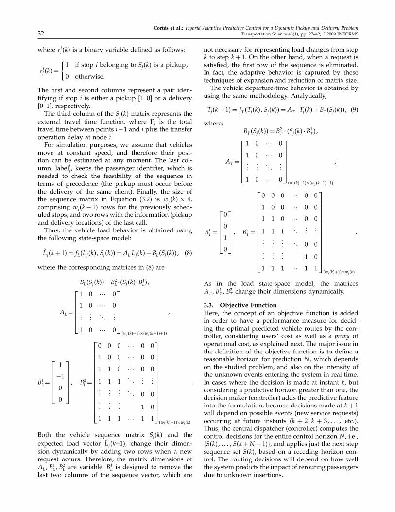
where r ij �k� is a binary variable defined as follows:

r ij �k� =

{1 if stop i belonging to Sj�k� is a pickup�

0 otherwise�

The first and second columns represent a pair iden-tifying if stop i is either a pickup 1 0 or a delivery0 1, respectively.The third column of the Sj�k� matrix represents the

external travel time function, where � ij is the total

travel time between points i−1 and i plus the transferoperation delay at node i.For simulation purposes, we assume that vehicles

move at constant speed, and therefore their posi-tion can be estimated at any moment. The last col-umn, labelij , keeps the passenger identifier, which isneeded to check the feasibility of the sequence interms of precedence (the pickup must occur beforethe delivery of the same client). Finally, the size ofthe sequence matrix in Equation (3.2) is wj�k� × 4,comprising wj�k − 1� rows for the previously sched-uled stops, and two rows with the information (pickupand delivery locations) of the last call.Thus, the vehicle load behavior is obtained using

the following state-space model:

L̂j �k + 1� = fL�Lj�k�� Sj�k�� = AL Lj�k� + BL�Sj�k��� (8)

where the corresponding matrices in (8) are

BL�Sj�k��=B2L ·�Sj �k�·B1

L��

AL =

⎡⎢⎢⎢⎢⎢⎣

1 0 ··· 0

1 0 ··· 0���

���� � �

���

1 0 ··· 0

⎤⎥⎥⎥⎥⎥⎦

�wj �k�+1�×�wj �k−1�+1�

�

B1L =

⎡⎢⎢⎢⎢⎢⎣

1

−1

0

0

⎤⎥⎥⎥⎥⎥⎦� B2

L =

⎡⎢⎢⎢⎢⎢⎢⎢⎢⎢⎢⎢⎢⎢⎢⎢⎣

0 0 0 ··· 0 0

1 0 0 ··· 0 0

1 1 0 ··· 0 0

1 1 1� � �

������

������

���� � � 0 0

������

��� 1 0

1 1 1 ··· 1 1

⎤⎥⎥⎥⎥⎥⎥⎥⎥⎥⎥⎥⎥⎥⎥⎥⎦

�wj �k�+1�×wj �k�

�

Both the vehicle sequence matrix Sj�k� and theexpected load vector L̂j �k+1�, change their dimen-sion dynamically by adding two rows when a newrequest occurs. Therefore, the matrix dimensions ofAL�B1

L�B2L are variable. B1

L is designed to remove thelast two columns of the sequence vector, which are

not necessary for representing load changes from stepk to step k + 1. On the other hand, when a request issatisfied, the first row of the sequence is eliminated.In fact, the adaptive behavior is captured by thesetechniques of expansion and reduction of matrix size.The vehicle departure-time behavior is obtained by

using the same methodology. Analytically,

�Tj�k + 1� = fT �Tj�k�� Sj�k�� = AT · Tj�k� + BT �Sj�k��� (9)

where:BT �Sj�k�� = B2

T · �Sj �k� · B1T ��

AT =

⎡⎢⎢⎢⎢⎢⎣

1 0 ··· 0

1 0 ··· 0���

���� � �

���

1 0 ··· 0

⎤⎥⎥⎥⎥⎥⎦

�wj �k�+1�×�wj �k−1�+1�

�

B1T =

⎡⎢⎢⎢⎢⎢⎣0

0

1

0

⎤⎥⎥⎥⎥⎥⎦� B2

T =

⎡⎢⎢⎢⎢⎢⎢⎢⎢⎢⎢⎢⎢⎢⎢⎢⎣

0 0 0 ··· 0 0

1 0 0 ··· 0 0

1 1 0 ··· 0 0

1 1 1� � �

������

������

���� � � 0 0

������

��� 1 0

1 1 1 ··· 1 1

⎤⎥⎥⎥⎥⎥⎥⎥⎥⎥⎥⎥⎥⎥⎥⎥⎦

�wj �k�+1�×wj �k�

�

As in the load state-space model, the matricesAT �B1

T �B2T change their dimensions dynamically.

3.3. Objective FunctionHere, the concept of an objective function is addedin order to have a performance measure for decid-ing the optimal predicted vehicle routes by the con-troller, considering users’ cost as well as a proxy ofoperational cost, as explained next. The major issue inthe definition of the objective function is to define areasonable horizon for prediction N , which dependson the studied problem, and also on the intensity ofthe unknown events entering the system in real time.In cases where the decision is made at instant k, butconsidering a predictive horizon greater than one, thedecision maker (controller) adds the predictive featureinto the formulation, because decisions made at k + 1will depend on possible events (new service requests)occurring at future instants (k + 2� k + 3� � � � � etc.).Thus, the central dispatcher (controller) computes thecontrol decisions for the entire control horizon N , i.e.,�S�k�� � � � � S�k + N − 1��, and applies just the next stepsequence set S�k�, based on a receding horizon con-trol. The routing decisions will depend on how wellthe system predicts the impact of rerouting passengersdue to unknown insertions.

Cortés et al.: Hybrid Adaptive Predictive Control for a Dynamic Pickup and Delivery ProblemTransportation Science 43(1), pp. 27–42, © 2009 INFORMS 33

The objective function for a generic prediction hori-zon N can be written as follows:

MinS�k�

J =N∑

t=1

F∑j=1

H�k+t�∑h=1

p�T �k+t�h

(�Cj �k + t� − Cj�k + t − 1���Sj �k+t−2��h

)�

(10)

Cj�k+t��Sj �k+t−2��h

=wj �k+t−1�∑

i=1

{L̂i−1

j �k+t�+1��T ij �k+t�− �T i−1

j �k+t��︸ ︷︷ ︸Jtravel time

+r ij �k+t−1� ��T i

j �k+t�−T 0j �k+t��︸ ︷︷ ︸

Jwaiting time

}∣∣∣∣Sj �k+t−2��h

� (11)

where k + t is the instant at which the tth requestenters the system, measured from time interval k.H�k + t� is the number of probable requests at instantk + t, p

�T �k+t�h is the probability of occurrence of the

hth request type (associated with a specific pair ofzones, as discussed later in this section) during timeinterval �T �k + t�, noting that �T �k + t� specifiesthe time interval to which time step k + t belongs.Cj�k + t��Sj �k+t−2��h in Equation (11) is a function associ-ated with vehicle j at instant k + t, which depends onthe decision sequence Sj�k + t −1�, given the previousknown sequence Sj�k + t − 2� associated with a poten-tial request h with probability p

�T �k+t�h . wj�k + t − 1�

is the number of stops estimated for vehicle j insequence Sj�k + t − 1�. Cj�k + t�, as shown in Equa-tion (11), can be split into two pieces: a travel time(Jtravel time� and a waiting time (Jwaiting time� component.Both components are written as functions of the loadand departure time. The former is computed as thedifference between the departure time of consecutivestops, multiplied by the vehicle load (represented bythe number of passengers plus the vehicle driver),whereas the latter considers the customers’ waitingtime while each vehicle moves on each segment ofits assigned route. For the sake of flexibility and eco-nomic consistency, the waiting cost component isweighted by a coefficient, . Analytically, L̂i−1

j �k + t�denotes the expected load over the segment from stopi − 1 to i; the difference �T i

j �k + t� − �T i−1j �k + t� mea-

sures the expected vehicle travel time on segment�i − 1� i�, including the transfer delay at node i; andthe difference �T i

j �k + t� − T 0j �k + t� measures the vehi-

cle expected travel time to reach stop i from its currentposition plus the expected transfer delay at node i.r ij �k + t − 1� corresponds to the same binary variableused to identify pickup and delivery points in thesequence expression (3.2), but in this case is associ-ated with the future sequence Sj�k + t − 1�. In the con-text of the objective function formulation, this binaryvariable can be interpreted as a waiting time factor.

Note that in the first component of the objectivefunction expression in Equation (11), the expectedtravel time is weighted by L̂i−1

j �k + t� + 1. In sucha computation, the expected load captures the usercost associated with travel time, whereas the addedone roughly incorporates a proxy for the operationalcost through the total time traveled by vehicles, eventhough some of them do not carry any passenger oncertain segments of their routes.The probabilities of occurrence of each scenario

p�T �k+t�h are parameters in the objective function, andthey are computed based on either real-time data, his-torical data, or a combination of both. In this particu-lar application, we use a simple way to compute theseprobabilities from historical data (offline implemen-tation). To do that, let us define the call mass centeras the geographical location of the most likely callto occur during a specific time period, and within aspecific area. As described in the problem formula-tion, what we really need is the probability that theexpected new request will occur between two spe-cific zones (pickup and delivery) within a certain timeinterval.In order to apply this methodology, the zone of

study has to be split into smaller subareas (clusters).How to choose the zoning will depend upon thedemand intensity associated with each specific prob-lem. The probability that a new call will appear fora specific pair of clusters h� �1� � � � �H�k + t�� within atime interval �T �k + t� is computed using the follow-ing expression:

p�T �k+t�h = N

�T �k+t�h∑H�k+t�

g=1 N�T �k+t�g

� (12)

where N�T �k+t�h is the total number of travel requests

belonging to a specific origin-destination pair ofclusters h over a set of pairs �1� � � � �H�k + t��,within a specific time interval �T �k + t�. Note that∑H�k+t�

h=1 p�T �k+t�h = 1, as expected.

With regard to the step size to be used in the predic-tion, George and Powell (2005) develop and discussmany interesting methods to incorporate a good esti-mate of optimal step size (such as a Kalman filter). Werealize that none of these methods properly replicatethe DPDP conditions, considering that in additionto representing a good estimate of the time betweencalls, what we really want to calibrate is a parame-ter for optimizing the system performance functionover time, which can lead to the optimal routing strat-egy including future information. To do that, a sen-sitivity analysis was conducted from simulated datato find the step-size value that minimizes the objec-tive function for more than one step ahead. It is veryimportant to highlight the fact that these variablesare continuous; nonoptimal behavior could occur if

Cortés et al.: Hybrid Adaptive Predictive Control for a Dynamic Pickup and Delivery Problem34 Transportation Science 43(1), pp. 27–42, © 2009 INFORMS

they are not properly adjusted by sensitivity analy-sis. For the two-steps-ahead application (see §4), thisparameter is denoted by � ; as discussed above, phys-ically it represents the expected time for a predictedrequest to happen. However, what � really representsis the best instant for inserting the future expected callin order to optimize the routing scheme. In general,these parameters are tunable for each step ahead ofprediction.In the context of this paper, we compare a myopic

strategy (one-step-ahead) with the two-steps-aheadpredictive approach that includes future informationfrom the system to show the improvements in rout-ing when considering a predictive component in therouting decisions under a DPDP system.The one-step-ahead strategy means that the pre-

diction horizon is N = 1, and H�k + 1� = 1 becausethe new requirement is one and known, and there-fore its probability is equal to 1. This results in thefollowing expression for the objective function usingEquation (10):

MinS�k�

J =1∑

t=1

F∑j=1

H�k+t�=1∑h=1

p�T �k+t�h �k + t�

· �Cj�k + t� − Cj�k + t − 1���Sj �k+t−2��h

=F∑

j=1

=1︷ ︸︸ ︷p

�T �k+1�1 �k + 1� ·�Cj�k + 1� − Cj�k���Sj �k−1��1

=F∑

j=1

(Cj�k + 1� −

knownconstant︷ ︸︸ ︷Cj�k�

)∣∣∣Sj �k−1��1

(13)

where

Cj�k+1��Sj �k−1��1

=wj �k�∑i=1

{L̂i−1

j �k+1�+1��T ij �k+1�− �T i−1

j �k+1��︸ ︷︷ ︸Jtravel time

+r ij �k� ��T i

j �k+1�−T 0j �k+1��︸ ︷︷ ︸

Jwaiting time

}∣∣∣∣Sj �k−1��1

(14)

Note that the difference �Cj�k + 1� − Cj�k���Sj �k−1��1 isevaluated considering the control action in the pre-vious instant, represented by Sj�k − 1�. Conceptu-ally, J represents the insertion cost when the systemaccepts a new call, computed in real time and consid-ering the entire vehicle fleet.The two-steps-ahead prediction’s objective function

is different from the previous one, because it includesa prediction of where the following call is going tofall, and with what probability. The controller selects

the vehicle’s sequence that minimizes the general two-steps-ahead objective function, which is as follows,

MinS�k�

J

=2∑

t=1

F∑j=1

H�k+t�∑h=1

p�T �k+t�h �k+t�

·�Cj�k+t�−Cj�k+t−1��∣∣Sj �k+t−2��h

=F∑

j=1

[Cj�k+1�

∣∣Sj �k−1��1

−Cj�k�

+H�k+2�∑

h=1

p�T �k+2�h �k+2�·Cj�k+2�

∣∣Sj �k��h

−

=1︷ ︸︸ ︷H�k+2�∑

h=1

p�T �k+2�h �k+2�·

independent of h︷ ︸︸ ︷Cj�k+1�

∣∣Sj �k−1��1

]

=F∑

j=1

[H�k+2�∑h=1

p�T �k+2�h �k+2�·Cj�k+2�

∣∣Sj �k��h

−knownconstant︷ ︸︸ ︷Cj�k�

]�

(15)

where

Cj�k+2��Sj �k��h

=wj �k+1�∑

i=1

{L̂i−1

j �k+2�+1��T ij �k+2�− �T i−1

j �k+2��︸ ︷︷ ︸Jtravel time

+r ij �k+1� ��T i

j �k+2�−T 0j �k+2��︸ ︷︷ ︸

Jwaiting time

}∣∣∣∣Sj �k��h

� (16)

3.4. Solution MethodTraditional optimization methods are not very effi-cient and, in most cases, useless for solving prob-lems like the one-step- and two-steps-ahead formu-lations presented above. This is mostly due to thehigh nonlinearity of the objective function expres-sions, in addition to the hybrid (discrete-continuous)nature of the variables. The optimization problem forboth one-step- and two-steps-ahead strategies couldbe solved by using explicit enumeration (EE) that con-siders all feasible insertion solutions whenever a callrequest enters the system. However, this inefficientmethod is neither appropriate for a large vehicle fleetnor for long prediction horizons, due to a compu-tational capacity constraint. For those scenarios, theapplication of such control algorithms solved with EEis not feasible in real-time routing. Instead, we proposea new ad hoc algorithm to solve the mixed-integerproblem behind the DPDP formulation proposed here.

Cortés et al.: Hybrid Adaptive Predictive Control for a Dynamic Pickup and Delivery ProblemTransportation Science 43(1), pp. 27–42, © 2009 INFORMS 35

The scheme is based on the particle swarm optimiza-tion (PSO) algorithm, which is a new type of evo-lutionary computation method that has performedquite well in previous applications, not only in termsof solution accuracy, but also in computation timesavings (Kennedy and Eberhart 2001). PSO has beeninspired by the social behavior of animals and insects,specifically on the behavior of a swarm of particlesover a multidimensional search space.After reviewing the literature, we highlight Coelho,

de Moura Oliveira, and Cunha (2005), who presenta predictive controller based on recursive linear mod-els where the optimization problem is solved by PSO.A good performance of PSO is shown in compari-son with genetic algorithms (GA) and classical quasi-Newton methods. Wang and Xiao (2005) describe aPSO-based predictive controller based on a radialbasis function (RBF) neural network model, obtain-ing slightly better results than those from GA and aquasi-Newton method. In the context of vehicle rout-ing, Zhu et al. (2006) propose a PSO scheme to solvea static vehicle-routing problem with time windows.The effectiveness, in terms of precision and compu-tational time, is shown by experimental results. Next,a description of the basic PSO algorithm is presented,to close the section with a detailed description of theproposed PSO-based algorithm for the DPDP.

PSO Algorithm. The PSO algorithm, used to solvecomplex nonlinear optimization problems, consists ofa particle swarm, which represents a population ofcandidate solutions. The particles are initialized ran-domly, and then move iteratively within the searchspace in order to find new solutions. The particleshave a fitness associated with the solution quality,usually given by the objective function to be opti-mized. Each particle is characterized by a position xi

(i is the index of the particle) and a velocity vi (bothare d-dimensional, where d is the dimension of thesolution vector). Each particle records its best previ-ous position x#

i �t� and the best position among allthe particles belonging to the swarm, namely x∗�t�,with t representing the current iteration. The particlesare updated according to their cognitive and socialbehavior from the following equations:

vi�t + 1� = � · vi�t� + c1 · �1 · �x#i �t� − xi�t��

+ c2 · �2 · �x∗�t� − xi�t���

xi�t + 1� = xi�t� + vi�t + 1��

(17)

where � is the inertia factor, c1 is the self-cognitiveconstant, and c2 represents the social component fac-tor (��c1� c2 > 0 are tuning parameters). Furthermore,�1 and �2 are uniformly distributed random num-bers in the range �0�1�, which help us preserve thediversity of the swarm. From Equations (17), parti-cles move according to their inertia, their experience,

and the experience of the most successful particle ofthe swarm. The search is conducted over a subset ofthe entire space (depending on the problem) to effec-tively guide the particles in the search space towardsthe optimum by keeping the velocity clamped insidea predefined range.The above description of PSO was originally con-

ceived for solving continuous problems. In our appli-cation, we completely adapted the PSO code in orderto add integer variables in the solution. Next, the spe-cific PSO we developed to solve the DPDP problemis described.

Proposed PSO Algorithm for Solving the DPDP.The proposed algorithm based on PSO utilizes par-ticles that belong to R2. For a new call requestingservice, the method finds the best insertion positionsfor the new pickup and delivery points along a cer-tain vehicle sequence. The algorithm is run for eachvehicle, to finally apply the new sequence to the vehi-cle showing the lowest insertion cost as based on theobjective function. In this problem, a particle is associ-ated with an insertion within a sequence for a specificvehicle.Let us consider a vehicle j with an associated

sequence Sj�k−1�. When a new call comes up at k, thePSO algorithm generates possible sequences S�

j �k�,with each one associated with a particle that finallydetermines the insertion position of the incoming call� = �pu�de� within the sequence, where pu corre-sponds to the pickup, and de to the delivery. Thus, asequence generated by PSO is given by

S�j �k�

=

⎡⎢⎢⎢⎢⎢⎢⎢⎢⎢⎢⎢⎢⎢⎢⎢⎢⎢⎣

r1j �k� 1−r1j �k� � 1j �k� label1j �k�

������

������

rpuj �k� 1−r

puj �k� �

puj �k� labelpuj �k�

������

������

rdej �k� 1−rdej �k� � dej �k� labeldej �k�

������

������

rwj �k�

j �k� 1−rwj �k�

j �k� �wj �k�

j �k� labelwj �k�

j �k�

⎤⎥⎥⎥⎥⎥⎥⎥⎥⎥⎥⎥⎥⎥⎥⎥⎥⎥⎦

wj �k�×4

�

(18)

where the puth row and deth row are the positions ofthe new pickup and delivery, respectively. Note thateach potential sequence in Equation (18) must be fea-sible in terms of precedence. Every particle providedby the PSO is two dimensional (both componentsare continuous) and has an associated insertion pair� = �pu�de�. Because the particles are real pairs, eachcomponent is approximated to the next integer. Whenparticles are either initialized or updated, they might

Cortés et al.: Hybrid Adaptive Predictive Control for a Dynamic Pickup and Delivery Problem36 Transportation Science 43(1), pp. 27–42, © 2009 INFORMS

not be feasible in terms of precedence, or becausethey could fall outside the allowable range (pickupout of 1�wj�k� − 1, and delivery out of 2�wj�k��.In these cases, the particles are repaired to get a feasi-ble sequence.The PSO algorithm specifies a function (detailed

in the description of the PSO-based algorithm to fol-low) to translate each particle into a feasible insertionposition, defining a possible sequence to be followedby the vehicle. An example is shown in (19).

Swarm

⇔

⎛⎜⎜⎜⎜⎜⎜⎜⎜⎜⎜⎜⎜⎜⎜⎝

Particle 1

Particle 2

Particle 3

Particle 4

Particle 5

Particle 6

Particle 7

⎞⎟⎟⎟⎟⎟⎟⎟⎟⎟⎟⎟⎟⎟⎟⎠

=

⎛⎜⎜⎜⎜⎜⎜⎜⎜⎜⎜⎜⎜⎜⎜⎝

x1 = �0�7�3�9�

x2 = �0�2�6�2�

x3 = �4�1�4�9�

x4 = �2�6�4�9�

x5 = �−0�8�7�4�

x6 = �3�1�1�1�

x7 = �1�9�3�2�

⎞⎟⎟⎟⎟⎟⎟⎟⎟⎟⎟⎟⎟⎟⎟⎠

⇔

⎛⎜⎜⎜⎜⎜⎜⎜⎜⎜⎜⎜⎜⎜⎜⎝

�1 = �pu1�de1�

�2 = �pu2�de2�

�3 = �pu3�de3�

�4 = �pu4�de4�

�5 = �pu5�de5�

�6 = �pu6�de6�

�7 = �pu7�de7�

⎞⎟⎟⎟⎟⎟⎟⎟⎟⎟⎟⎟⎟⎟⎟⎠

⇔

⎛⎜⎜⎜⎜⎜⎜⎜⎜⎜⎜⎜⎜⎜⎜⎝

�1�4�

�1�6�

�4�5�

�3�5�

�1�6�

�2�3�

�2�4�

⎞⎟⎟⎟⎟⎟⎟⎟⎟⎟⎟⎟⎟⎟⎟⎠

⇔

⎛⎜⎜⎜⎜⎜⎜⎜⎜⎜⎜⎜⎜⎜⎜⎜⎜⎜⎝

3+ → 1+ → 2+ → 3− → 1− → 2−

3+ → 1+ → 2+ → 1− → 2− → 3−

1+ → 2+ → 1− → 3+ → 3− → 2−

1+ → 2+ → 3+ → 1− → 3− → 2−

3+ → 1+ → 2+ → 1− → 2− → 3−

1+ → 3+ → 3− → 2+ → 1− → 2−

1+ → 3+ → 2+ → 3− → 1− → 2−

⎞⎟⎟⎟⎟⎟⎟⎟⎟⎟⎟⎟⎟⎟⎟⎟⎟⎟⎠

� (19)

In this example, for Particles 1, 4, and 7, a simplerounding up generates a feasible sequence in bothprecedence and allowable range. In the cases of Par-ticles 2 and 5, a simple rounding up generates asequence feasible in terms of precedence but outsidethe allowable range; thus, the sequence is repaired. ForParticles 3 and 6, a simple rounding up generates asequence within the allowable range, but unfeasiblein terms of precedence. Once again, the sequence isrepaired.

For all feasible particles, a PSO fitness value is eval-uated in terms of the corresponding objective func-tion as defined in Equation (10). Note that when asequence is unfeasible in terms of capacity, it is notrepaired; rather, a penalized fitness is used instead.Without loss of generality, the proposed algorithm

based on PSO is described for a two-steps-aheadhorizon. The algorithm is written as a function ofthree major procedures: GEN_PAR, REP_PAR, andMOD_PAR. With GEN_PAR the particles associatedwith potential sequences are randomly generated.REP_PAR takes the particles and generates their asso-ciated feasible sequences. Finally, MOD_PAR corre-sponds to the core of the evolutionary PSO algorithm,updating the particles for the next iteration accordingto the best previous solutions. The algorithm iteratesfirst at one-step-ahead and then at two-steps-ahead,as detailed below:

PSO-Based AlgorithmStep 0. Initialize parameters PSO, like n = number

of particles, � = inertia weight, c1 = cognitive weight,c2 = social weight.Step 1. Assume that the predefined sequence set

S�k − 1� is known. A new service request (call)enters the system. Then, the functions GEN_PAR andREP_GEN based on PSO are utilized to generaten potential sets of sequences S�l �k�, with l� 1�2� � � � �n(particles). Note that n/F particles are associatedwith each vehicle, which means that the insertion ofthe new call falls in the specific vehicle sequence (F isthe fleet size).Step 2. For each particle S�l �k�, consider H�k + 1�

probable requests. Then, GEN_PAR and REP_GENbased on PSO are applied to generate n potentialsequences S�m�k + 1��h, m� 1�2� � � � �n, for each proba-ble request pattern h� 1�2� � � � �H�k + 1�.Step 3. Provided that S�l �k� is known, evaluate

the fitness function C�k + 2��S�l �k��h − C�k + 1��S�k−1�,defined in Equations (14) and (16), for all potentialsequences S�m�k + 1��h. If S�m�k + 1��h is unfeasible forcapacity, penalize its fitness. Then, the best set of par-ticles S�∗

m�k + 1��h for h� 1�2� � � � �H�k + 1� associatedwith the minimum fitness function is selected.Step 4. If a tolerance criterion (maximum num-

ber of iterations of Steps 3 and 4) is satisfied, thenproceed to Step 5. Otherwise, update the positionand the velocity of all particles by using the func-tion MOD_PAR (evolutionary stage). With the func-tion REP_GEN, generate the sequences S�m�k + 1��h,m� 1�2� � � � �n for h� 1�2� � � � �H�k + 1� and go back toStep 3.Step 5. Given that S�l �k� is known, and by using

S�∗m�k + 1��h for h� 1� � � � �H�k + 1� obtained in Step 3,

evaluate the two-steps-ahead objective function (fit-ness) in Equation (15). If S�l �k� is unfeasible for capac-ity, penalize its fitness.

Cortés et al.: Hybrid Adaptive Predictive Control for a Dynamic Pickup and Delivery ProblemTransportation Science 43(1), pp. 27–42, © 2009 INFORMS 37

Step 6. From the fitness computed for each particleS�l �k�, l� 1�2� � � � �n, record the best sequence S�∗

l �k�.Step 7. If a tolerance criterion (maximum number

of iterations Steps 2 to 7) is satisfied, then STOP andS�∗

l �k� is the optimum. Otherwise, by using the func-tion MOD_PAR (evolutionary stage), update the posi-tion and the velocity of all particles for l� 1�2� � � � �n.By using REP_GEN, generate S�l �k�, l� 1�2� � � � �n, andgo back to Step 2.The detailed procedures involved in the algorithm

are explained next:

GEN_PARThis procedure is performed for the first iteration,t = 1.For every vehicle j , n/F particles are assigned.

Then, for every particle l associated with a given vehi-cle j , the following features are set:Initialize random positions and velocities for the

particles.

xl�1� = �x1l�1�� x2l�1���

�x1l�1�� x2l�1�� ∈ 0�wj�k� − 1 × 1�wj�k��

vl�1� = �v1l�1��v2l�1���(v1l�1��v2l�1�� ∈ −wj�k�/2�wj�k�/2

× −wj�k�/2�wj�k�/2�

REP_PARThis function is required to convert a particle l into afeasible sequence. Thus, for every particle l associatedwith a vehicle j , the repair procedure is as follows:

Round and repair particle out-of-range.

pul =max�min�x1l�t���wj�k� − 1��1��

del =min�max�x2l�t���2��wj�k���

If pul < del, then �l = �pul� del�.

Repair unfeasible particle in precedence.If pul > del, then y = �pul − del�/2, pul = �pul − y ,

del = del + y�, �l = �pul� del�.If pul = del, then del = min�wj�k��del + 1�, pul =

max�del − 1�1�, �l = �pul� del�.

Finally, depending on the case (one-step- or two-steps-ahead iteration), the sequence S�k� (or S�k + 1��associated with the particle l is S�l �k� (or S�l �k + 1��h�.MOD_PARThis function corresponds to the evolutionary stage ofthe PSO algorithm. Thus, for every particle l associ-ated with a vehicle j , the procedure is as follows (foriteration t + 1):

Update velocity:

vl�t + 1� = � · vl�t� + c1 · �1 · �x#l �t� − xl�t��

+ c2 · �2 · �x∗�t� − xl�t���

If velocity is saturated, then set

�v1l� v2l� ∈ −wj�k�/2�wj�k�/2 × −wj�k�/2�wj�k�/2�

Update position:

xl�t + 1� = xl�t� + vl�t��

where xl�t��vl�t� are the position and the velocity ofparticle l at iteration t, �1 and �2 are uniformly dis-tributed random numbers in the range �0�1�, � isthe inertia weight, c1 is the cognitive weight, c2 isthe social weight, x#

l �t� is the best previous positionreached for particle l, and x∗�t� is the best positionamong all particles belonging to the swarm.

4. Simulation Tests4.1. Experiment DescriptionA discrete-event system simulation is conducted for athree-hour period to evaluate the performance of theproposed dispatch control algorithm for a dynamicvehicle-routing system. The scheme considers a fleetof nine transit vehicles, each with a capacity for fourpassengers. Dispatch decisions are made in real-timeby the controller. Service requests are unknown; how-ever, the average system pattern is supposed to beknown from historical data, obtained from the aver-age demand measured over the preceding week.The simulation scenario is not real. However, the

demand patterns follow a heterogeneous distributioninspired by real data from the Origin-Destination Sur-vey in Santiago, Chile, 2001. We consider an urbanservice area of approximately 81 km2. Vehicles areassumed to travel straight between stops at an aver-age speed of 20 km/hr throughout the region. Thesimulation was performed over three time intervals ina representative work day during the morning peakhour, i.e., Tp = (7:00–7:59, 8:00–8:59, 9:00–9:59), and thedemand distribution was assumed to follow variouspatterns over the studied period, as discussed below.The objective of the experiments was to test the per-

formance of the predictive algorithm under differentconditions and modeling assumptions. One major fac-tor in the definition of the expected occurrence prob-ability of future service requests is the spatial (andtemporal) disaggregation of the total area (and timeperiod).Following the methodology, we generate historical

data assuming that 90% of the intervehicle trips occurin six pairs of sectors (H = 6). Therefore, we con-sider this subset of origin destination pairs for theobjective function computation. Next, the different ar-rival rates per geographic pair-interval were obtained,from which the corresponding occurrence probabili-ties were generated. For simplicity, we assumed that

Cortés et al.: Hybrid Adaptive Predictive Control for a Dynamic Pickup and Delivery Problem38 Transportation Science 43(1), pp. 27–42, © 2009 INFORMS

(0, 9) (3, 9) (6, 9) (9, 9)

(9, 6)

(9, 3)

(9, 0)(6, 0)(3, 0)(0, 0)

1

4

7 7 7

56

98

2 3

[Km]

[Km]

(0, 9) (3, 9) (6, 9) (9, 9)

(9, 6)

(9, 3)

(9, 0)(6, 0)(3, 0)(0, 0)

1

4 5 6

98

2 3

[Km]

[Km]

7:00–7:59 A.M. 8:00–8:59 A.M.

(0, 9) (3, 9) (6, 9) (9, 9)

(9, 6)

(9, 3)

(9, 0)(6, 0)(3, 0)(0, 0)

1

4 5 6

98

2 3

[Km]

[Km]

9:00–9:59 A.M.

P/D 5 6 9 P/D 5 6 9124

78

2

0.20

0.10

0.100.30

0.100.20

4578

P/D 53 6 91

0.30.2

0.10.1

0.2

0.1569

0.20 0.20

0.150.15

0.150.15

Figure 3 Origin-Destination Trip Patterns (Nine-Zone Division)Note. P\D: Pickup and delivery zones.

the probabilities do not change within each time inter-val, but they do from one interval to the next.First, we tested nine homogeneous zones where his-

torical data show that trips occur in the six most rel-evant interzonal origin-destination pairs, as shownin Figure 3. The probability associated with eachtrip pattern is in the table underneath each figure.For example, considering the schedule between 7:00and 7:59 a.m., the chance that a trip from Zone 1 toZone 5 occurs is 0.2 among all trips occurring every-where else within that time interval. The probability ofother trips between zones not considered among thesix most important pairs is assumed to be negligible.For this zoning desegregation, intrazonal trips wereassumed to be negligible too.A second experiment was to aggregate the spatial

area into four zones instead of the nine used in theprevious example, assuming the same trip patternsas above. Figure 4 shows the scheme associated with

(0, 9) (3, 9)

3 34 4

2

0.15

0.15 0.3

0.4

21 1

(6, 9) (9, 9)

(9, 6)

(9, 3)

(9, 0)(6, 0)(3, 0)(0, 0)

[Km]

[Km]

(0, 9) (3, 9) (6, 9) (9, 9)

(9, 6)

(9, 3)

(9, 0)(6, 0)(3, 0)(0, 0)

[Km]

[Km]

7:00–7:59 A.M. 8:00–8:59 A.M.

(0, 9) (3, 9) (6, 9) (9, 9)

(9, 6)

43

1 2

(9, 3)

(9, 0)(6, 0)(3, 0)(0, 0)

[Km]

[Km]

9:00–9:59 A.M.

P/D 2

1

3

4

0.14 0.120.230.51

P/D 11

3

30.13

0.29

0.29 0.29

P/D 2 44 2

3

4

Figure 4 Origin-Destination Trip Patterns (Four-Zone Division).Note. P\D: Pickup and delivery zones.

this second case. Note that intrazonal trip probabili-ties cannot be neglected in this case, due to the moreaggregated zoning.In terms of demand, 120 calls were generated over

the whole simulation period of three hours, accordingto a spatial and temporal distribution with the samebehavior as the historical pattern considered.A distribution for the time interval between suc-

cessive calls is also assumed in order to computetime-interval probabilities. In this case, we use anegative exponential distribution, with rates of 0.5[call/minute], 1 [call/minute], and 0.5 [call/minute]for the first, second, and third hours of simulation,respectively. In terms of spatial distribution, pickupand delivery points were generated randomly withineach corresponding zone in order to replicate thetrip pattern and probabilities shown in Figures 3 and4, depending on the experiment. Arbitrarily, vehicleswere initially located at the mass center of zones. This

Cortés et al.: Hybrid Adaptive Predictive Control for a Dynamic Pickup and Delivery ProblemTransportation Science 43(1), pp. 27–42, © 2009 INFORMS 39

assumption does not affect the final statistics of thetests, because a reasonable warm-up period was con-sidered. Thirty replications of each experiment wereconducted to obtain global statistics, as shown in §4.2.With regard to the objective function, = 1 was used,which means that the travel time is as important as thewaiting time in the objective function expression. Theone-step- and two-steps-ahead algorithms are thenevaluated and compared for both the four- and nine-zone spatial disaggregation cases. The PSO algorithmwith no swapping was implemented in Matlab ver-sion 7.0 with a Pentium IV processor. The parametersof PSO used in this first approach were � = 1, c1 = 2,c2 = 2.As introduced in the previous section, one relevant

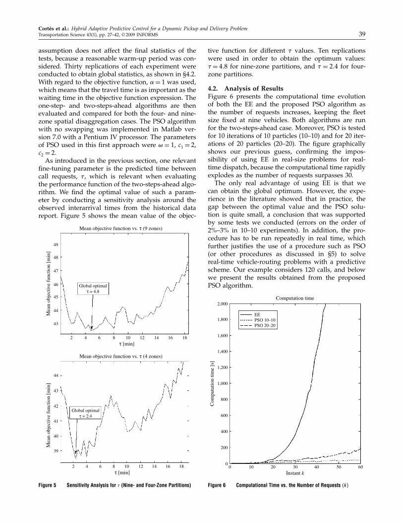
fine-tuning parameter is the predicted time betweencall requests, � , which is relevant when evaluatingthe performance function of the two-steps-ahead algo-rithm. We find the optimal value of such a param-eter by conducting a sensitivity analysis around theobserved interarrival times from the historical datareport. Figure 5 shows the mean value of the objec-

49

48

47

46

45

44

43

2 4 6 8 10 12 14 16 18τ [min]

Mean objective function vs. τ (9 zones)

Mea

n ob

ject

ive

func

tion

[min

]

Global optimalτ = 4.8

44

43

42

41

40

39

2 4 6 8 10 12 14 16 18τ [min]

Mean objective function vs. τ (4 zones)

Mea

n ob

ject

ive

func

tion

[min

]

Global optimalτ = 2.4

Figure 5 Sensitivity Analysis for � (Nine- and Four-Zone Partitions)

tive function for different � values. Ten replicationswere used in order to obtain the optimum values:� = 4�8 for nine-zone partitions, and � = 2�4 for four-zone partitions.

4.2. Analysis of ResultsFigure 6 presents the computational time evolutionof both the EE and the proposed PSO algorithm asthe number of requests increases, keeping the fleetsize fixed at nine vehicles. Both algorithms are runfor the two-steps-ahead case. Moreover, PSO is testedfor 10 iterations of 10 particles (10–10) and for 20 iter-ations of 20 particles (20–20). The figure graphicallyshows our previous guess, confirming the impos-sibility of using EE in real-size problems for real-time dispatch, because the computational time rapidlyexplodes as the number of requests surpasses 30.The only real advantage of using EE is that we

can obtain the global optimum. However, the expe-rience in the literature showed that in practice, thegap between the optimal value and the PSO solu-tion is quite small, a conclusion that was supportedby some tests we conducted (errors on the order of2%–3% in 10–10 experiments). In addition, the pro-cedure has to be run repeatedly in real time, whichfurther justifies the use of a procedure such as PSO(or other procedures as discussed in §5) to solvereal-time vehicle-routing problems with a predictivescheme. Our example considers 120 calls, and belowwe present the results obtained from the proposedPSO algorithm.

2,000

1,800

1,600

1,400

1,200

1,000

800

600

400

200

00 10 20 30 40 50 60

Instant k

Com

puta

tion

time

[s]

Computation time

EEPSO 10-10PSO 20-20

Figure 6 Computational Time vs. the Number of Requests �k�

Cortés et al.: Hybrid Adaptive Predictive Control for a Dynamic Pickup and Delivery Problem40 Transportation Science 43(1), pp. 27–42, © 2009 INFORMS

Table 1 PSO Computational Time and Performance Comparison Using Different Parameters for Four Zones and FourProbabilities

Total time(waiting+ travel) (min) Operation time (min) Computational time (sec)

Two step ahead Mean Std Mean Std Mean Std

5 iterations, 5 particles 46.76 4.41 182.61 6.17 589�6 98�6210 iterations, 10 particles 41.71 4.97 178.73 8.42 1�737�3 129�4415 iterations, 15 particles 41.02 4.30 178.35 6.18 2�559�6 576�92

We have chosen the mean and standard devia-tion values of total travel and waiting times to mea-sure the system performance in terms of user levelof service. Additionally, the average total time spentby a vehicle in the system is also reported as aproxy of the average operational cost. In Table 1below, we show the PSO computational time andperformance comparison using different parameters(iterations-particles) for four zones and four probabil-ities. As expected, Table 1 shows a trade-off betweenthe solution accuracy and the PSO computational timefor the two-steps-ahead algorithm.From the table, it seems reasonable to use 10 itera-

tions and 10 particles (10–10) in the following exper-iments. Note that in terms of solution quality, we donot obtain too much improvement (41.71 versus 41.02and 178.73 versus 178.35) for adding five more par-ticles and iterations. However, in computation time,the cost of this change is quite considerable. In Fig-ure 6, we can graphically see the low computationaleffort needed to run the 10–10 PSO algorithm for thetwo-steps-ahead case.From such an observation, in Tables 2, 3, and 4,

the user and operator performance indicators for the30 replications of the PSO algorithm with 10 particlesand 10 iterations are reported. These values capturethe differences of running both algorithms (one-step-ahead versus two-steps-ahead) for both experi-ments, nine zones (six probabilities), and four zones(four probabilities), respectively. A warm-up periodof 20 minutes at both sides (the start and end of thesimulation period) was considered to measure systemperformance under steady-state conditions.

Table 2 One-Step-Ahead and Two-Steps-Ahead PerformanceComparison Nine Zones, Six Probabilities

Waiting Travel Totaltime (min) time (min) time (min)

PSO Mean Std Mean Std Mean Std

One step ahead 21.70 2.22 23.88 1.51 45.58 3.47Two step ahead 20.03 3.33 23.17 1.33 43.20 4.23

Savings 1.67 0.71 2.38Improv. % 7.68 2.98 5.22

Tables 2 and 3 show the performance of the twoalgorithms over the whole three-hour period (exclud-ing the warm-up interval). From the results shownin the tables above, we appreciate that the predictive(two-steps-ahead) algorithm systematically performsbetter than the one-step-ahead algorithm, supportingour initial guess regarding the necessity of adding apredictive component into the real-time routing algo-rithms applied to this kind of system.The most important savings from the predictive

approach comes from the waiting time component(13.23% in the best case). From this result, we caninfer that most prediction benefits are due to avoidingextra waiting at future pickup points on scheduledvehicle sequences, which is quite manageable by thedispatcher once he can make routing decisions basedupon future potential requests.From the example, improvements in travel time

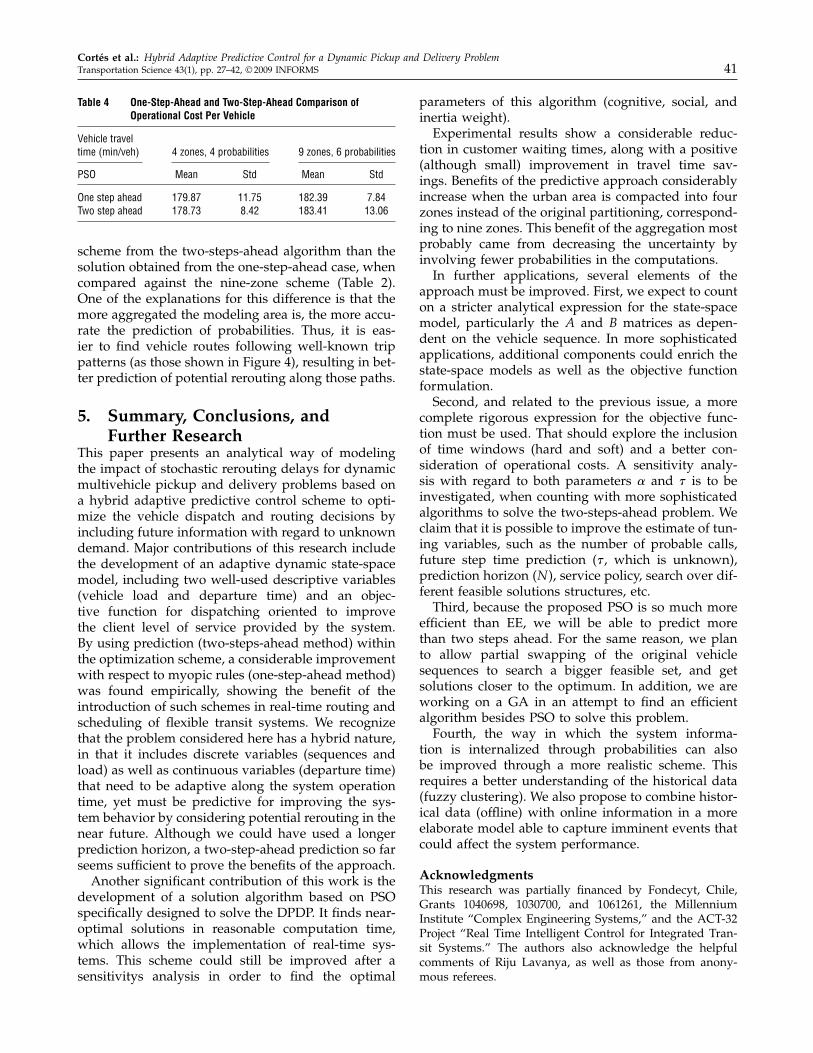
from predictive algorithms are lower than thoseobtained for waiting time (5.38% in the best case).In addition, there is absolutely no observable improve-ment in operational cost; it remains practically con-stant, as shown in Table 4. We hypothesize that themagnitude of the travel time benefits as well as sav-ings in operational cost could be improved by con-sidering further adjustments of the objective functionformulation. Actually, the current objective functionversion does not take into account the real weight ofthe operational cost compared with customer levelof service in terms of waiting and travel time as partof the specification (see §5 for discussion of this topicas part of planned further research).Moreover, it seems that the most aggregated zoning

scenario (Table 3) results in a more efficient routing

Table 3 One-Step-Ahead and Two-Steps-Ahead PerformanceComparison Four Zones, Four Probabilities

Waiting Travel Totaltime (min) time (min) time (min)

PSO Mean Std Mean Std Mean Std

One step ahead 21.92 4.52 23.98 1.53 45.90 5.33Two step ahead 19.02 3.36 22.69 1.46 41.71 4.58

Savings 2.74 1.29 4.19Improv. % 13.23 5.38 10.05

Cortés et al.: Hybrid Adaptive Predictive Control for a Dynamic Pickup and Delivery ProblemTransportation Science 43(1), pp. 27–42, © 2009 INFORMS 41

Table 4 One-Step-Ahead and Two-Step-Ahead Comparison ofOperational Cost Per Vehicle

Vehicle traveltime (min/veh) 4 zones, 4 probabilities 9 zones, 6 probabilities

PSO Mean Std Mean Std

One step ahead 179.87 11.75 182.39 7.84Two step ahead 178.73 8.42 183.41 13.06

scheme from the two-steps-ahead algorithm than thesolution obtained from the one-step-ahead case, whencompared against the nine-zone scheme (Table 2).One of the explanations for this difference is that themore aggregated the modeling area is, the more accu-rate the prediction of probabilities. Thus, it is eas-ier to find vehicle routes following well-known trippatterns (as those shown in Figure 4), resulting in bet-ter prediction of potential rerouting along those paths.

5. Summary, Conclusions, andFurther Research

This paper presents an analytical way of modelingthe impact of stochastic rerouting delays for dynamicmultivehicle pickup and delivery problems based ona hybrid adaptive predictive control scheme to opti-mize the vehicle dispatch and routing decisions byincluding future information with regard to unknowndemand. Major contributions of this research includethe development of an adaptive dynamic state-spacemodel, including two well-used descriptive variables(vehicle load and departure time) and an objec-tive function for dispatching oriented to improvethe client level of service provided by the system.By using prediction (two-steps-ahead method) withinthe optimization scheme, a considerable improvementwith respect to myopic rules (one-step-ahead method)was found empirically, showing the benefit of theintroduction of such schemes in real-time routing andscheduling of flexible transit systems. We recognizethat the problem considered here has a hybrid nature,in that it includes discrete variables (sequences andload) as well as continuous variables (departure time)that need to be adaptive along the system operationtime, yet must be predictive for improving the sys-tem behavior by considering potential rerouting in thenear future. Although we could have used a longerprediction horizon, a two-step-ahead prediction so farseems sufficient to prove the benefits of the approach.Another significant contribution of this work is the

development of a solution algorithm based on PSOspecifically designed to solve the DPDP. It finds near-optimal solutions in reasonable computation time,which allows the implementation of real-time sys-tems. This scheme could still be improved after asensitivitys analysis in order to find the optimal

parameters of this algorithm (cognitive, social, andinertia weight).Experimental results show a considerable reduc-

tion in customer waiting times, along with a positive(although small) improvement in travel time sav-ings. Benefits of the predictive approach considerablyincrease when the urban area is compacted into fourzones instead of the original partitioning, correspond-ing to nine zones. This benefit of the aggregation mostprobably came from decreasing the uncertainty byinvolving fewer probabilities in the computations.In further applications, several elements of the

approach must be improved. First, we expect to counton a stricter analytical expression for the state-spacemodel, particularly the A and B matrices as depen-dent on the vehicle sequence. In more sophisticatedapplications, additional components could enrich thestate-space models as well as the objective functionformulation.Second, and related to the previous issue, a more

complete rigorous expression for the objective func-tion must be used. That should explore the inclusionof time windows (hard and soft) and a better con-sideration of operational costs. A sensitivity analy-sis with regard to both parameters and � is to beinvestigated, when counting with more sophisticatedalgorithms to solve the two-steps-ahead problem. Weclaim that it is possible to improve the estimate of tun-ing variables, such as the number of probable calls,future step time prediction (� , which is unknown),prediction horizon (N ), service policy, search over dif-ferent feasible solutions structures, etc.Third, because the proposed PSO is so much more

efficient than EE, we will be able to predict morethan two steps ahead. For the same reason, we planto allow partial swapping of the original vehiclesequences to search a bigger feasible set, and getsolutions closer to the optimum. In addition, we areworking on a GA in an attempt to find an efficientalgorithm besides PSO to solve this problem.Fourth, the way in which the system informa-

tion is internalized through probabilities can alsobe improved through a more realistic scheme. Thisrequires a better understanding of the historical data(fuzzy clustering). We also propose to combine histor-ical data (offline) with online information in a moreelaborate model able to capture imminent events thatcould affect the system performance.

AcknowledgmentsThis research was partially financed by Fondecyt, Chile,Grants 1040698, 1030700, and 1061261, the MillenniumInstitute “Complex Engineering Systems,” and the ACT-32Project “Real Time Intelligent Control for Integrated Tran-sit Systems.” The authors also acknowledge the helpfulcomments of Riju Lavanya, as well as those from anony-mous referees.

Cortés et al.: Hybrid Adaptive Predictive Control for a Dynamic Pickup and Delivery Problem42 Transportation Science 43(1), pp. 27–42, © 2009 INFORMS

ReferencesBemporad, A., M. Morari. 1999. Control of systems integrating

logic, dynamics and constraints. Automatica 35 407–427.Bemporad, A., F. Borrelli, M. Morari. 2002. Model predictive control

based on linear programing. The explicit solution. IEEE Trans.Automatic Control 47(12) 1974–1985.

Bertsimas, D., G. van Ryzin. 1991. A stochastic and dynamic vehiclerouting problem in the Euclidean plane. Oper. Res. 39 601–615.

Bertsimas, D., G. van Ryzin. 1993a. Stochastic and dynamic vehiclerouting problem in the Euclidean plane with multiple capaci-tated vehicles. Oper. Res. 41 60–76.

Bertsimas, D., G. van Ryzin. 1993b. Stochastic and dynamic vehiclerouting with general demand and interarrival time distribu-tions. Appl. Probab. 25 947–978.

Coelho, J. P., P. B. de Moura Oliveira, J. B. Cunha. 2005. Greenhouseair temperature predictive control using the particle swarmoptimisation algorithm. Comput. Electronics in Agriculture 49330–344.

Cortés, C. E., R. Jayakrishnan. 2004. Analytical modeling of stochas-tic rerouting delays for dynamic multi-vehicle pickup anddelivery problems. The Fifth Triennial Symposium on Transporta-tion Analysis, TRISTAN V. Le Gosier, Guadalupe, 13–18 June.

Desrosiers, J., F. Soumis, Y. Dumas. 1986. A dynamic programmingsolution of a large-scale single-vehicle dial-a-ride with timewindows. Amer. J. Math. Management Sci. 6 301–325.

Dial, R. 1995. Autonomous dial a ride transit—Introductoryoverview. Transportation Res.—Part C 3 261–275.

Dréo, J., A. Pétrowski, P. Siarry, E. Taillard. 2006. Metaheuristics forHard Optimization Methods and Case Studies. Springer-Verlag,Berlin.

Figliozzi, M., H. Mahmassani, P. Jaillet. 2007. Pricing in dynamicvehicle routing problems. Transportation Sci. 41(3) 302–318.

Gendreau, M., F. Guertin, J. Potvin, E. Taillard. 1999. Parallel tabusearch for real-time vehicle routing and dispatching. Trans-portation Sci. 33 381–390.

George, A., W. Powell. 2005. Adaptive stepsizes for recursive esti-mation with applications in approximate dynamic program-ming. http://www.castlelab.princeton.edu/.

Godfrey, G., W. B. Powell. 2002. An adaptive dynamic program-ming algorithm for stochastic resource allocation problems I:Single period travel times. Transportation Sci. 36 21–39.

Haghani, A., S. Jung. 2005. A dynamic vehicle routing problem withtime-dependent travel times. Comput. Oper. Res. 32 2959–2986.

Ichoua, S., M. Gendreau, J. Y. Potvin. 2006. Exploiting knowledgeabout future demands for real-time vehicle dispatching. Trans-portation Sci. 40(2) 211–225.

Jaw, J., A. Odoni, H. Psaraftis, N. Wilson. 1986. A heuristic algorithmfor the multivehicle many-to-many advance-request dial-a-rideproblem. Transportation Res. B: Methodological 20(3) 243–257.

Jih, W., J. Yung-Jen. 1999. Dynamic vehicle routing using hybridgenetic algorithms. Proc. IEEE Internat. Conf. Robotics & Automa-tion, May, Detroit, MI, 453–458.

Kennedy, J., R. Eberhart. 2001. Swarm Intelligence. MorganKaufmann Publishers, San Francisco.

Larsen, A. 2000. The dynamic vehicle routing problem, Ph.D. thesis,Technical University of Denmark, Denmark.

Madsen, O., H. Raven, J. Rygaard. 1995. A Heuristics algorithm fora dial-a-ride problem with time windows, multiple capacities,and multiple objectives. Ann. Oper. Res. 60 193–208.

Malandraki, C., M. S. Daskin. 1992. Time dependent vehicle routingproblems: Formulations, properties and heuristic algorithms.Transportation Sci. 26 185–200.

Montemanni, R., L. M. Gambardella, A. E. Rizzoli, A. Donati. 2005.Ant colony system for a dynamic vehicle routing problem.J. Combin. Optim. 10(4) 327–343.

Osman, M., M. Abo-Sinna, A. Mousa. 2005. An effective geneticalgorithm approach to multiobjective routing problems(MORPs). Appl. Math. Comput. 163 769–781.

Powell, W. B. 1988. A comparative review of alternative algorithmsfor the dynamic vehicle allocation problem. B. L. Golden, A. A.Assad, eds. Vehicle Routing Methods and Studies. North-Holland,Amsterdam.

Powell, W. B., P. Jaillet, A. Odoni. 1995. Stochastic and dynamicnetworks and routing. M. Ball, T. Magnanti, C. Monma,G. Nemhauser, eds. Network Routing. A Handbook in Opera-tions Research and Management Science, Vol. 8. North-Holland,Amsterdam, 141–296.

Psaraftis, H. 1980. A dynamic programming solution to the singlemany-to-many immediate request dial-a-ride problem. Trans-portation Sci. 14(2) 130–154.

Psaraftis, H. 1988. Dynamic vehicle routing problems. B. L. Golden,A. A. Assad, eds. Vehicle Routing Methods and Studies, North-Holland, Amsterdam, 223–248.

Savelsbergh, M., M. Sol. 1995. The general pickup and deliveryproblem. Transportation Sci. 29(1) 17–29.

Skrlec, D., M. Filipec, S. Krajcar. 1997. A heuristic modification ofgenetic algorithm used for solving the single depot capacitatedvehicle routing problem. Proc. Intelligent Inform. Systems, IIS’97. Washington, D.C. IEEE, 184–188.

Spivey, M., W. B. Powell. 2004. The dynamic assignment problem.Transportation Sci. 38(4) 399–419.

Swihart, M. R., J. D. Papastavrou. 1999. A stochastic and dynamicmodel for the single-vehicle pick-up and delivery problem.Eur. J. Oper. Res. 114 447–464.

Tarantilis, C. 2005. Solving the vehicle routing problem with adap-tive memory programming methodology. Comput. Oper. Res. 322309–2327.

Thomas, B., C. White, III. 2004. Anticipatory route selection. Trans-portation Sci. 38(4) 473–487.

Tighe, A., F. Smith, G. Lyons. 2004. Priority based solver for a real-time dynamic vehicle routing. IEEE Internat. Conf. Systems, Manand Cybernetics. IEEE, 6237–6242.

Topaloglu, H., W. Powell. 2005. A distributed decision-makingstructure for dynamic resource allocation using non linearfunctional approximations. Oper. Res. 53(2) 281–297.

Topaloglu, H., W. Powell. 2007. Incorporating pricing decisions intothe stochastic dynamic fleet management problem. Transporta-tion Sci. 41(3) 281–301.

Toth, P., D. Vigo. 2003. The granular tabu search and its applica-tion to the vehicle-routing problem. INFORMS J. Comput. 15(4)333–346.

Wang, X., J. Xiao. 2005. PSO-based model predictive control fornonlinear processes. Lecture Notes in Computer Science, Vol. 3611.Springer-Verlag, Berlin, 196–203.

Wilson, N., N. Colvin. 1977. Computer control of Rochester dial-a-ride system. Report R77-31, Department of Civil Engineering,M.I.T., Cambridge, MA.

Wilson, N., H. Weissberg. 1976. Advanced dial-a-ride algorithmsresearch project: Final report. Report R76-20, Department ofCivil Engineering, M.I.T., Cambridge, MA.

Zhu, Q., L. Qian, Y. Li, S. Zhu. 2006. An improved particleswarm optimization algorithm for vehicle routing problemwith time windows. IEEE Congress on Evolutionary Compu-tation, Vancouver, July 16–21.