HPI Future SOC Lab : Proceedings 2013 - Hasso-Plattner-Institut

Technische Berichte Nr. 88

des Hasso-Plattner-Instituts für Softwaresystemtechnik an der Universität Potsdam

HPI Future SOC Lab: Proceedings 2013Christoph Meinel, Andreas Polze, Gerhard Oswald, Rolf Strotmann, Ulrich Seibold, Bernhard Schulzki (Hrsg.)

ISBN 978-3-86956-282-7ISSN 1613-5652

Technische Berichte des Hasso-Plattner-Instituts für Softwaresystemtechnik an der Universität Potsdam

Bibliografische Information der Deutschen Nationalbibliothek Die Deutsche Nationalbibliothek verzeichnet diese Publikation in der Deutschen Nationalbibliografie; detaillierte bibliografische Daten sind im Internet über http://dnb.dnb.de/ abrufbar. Universitätsverlag Potsdam 2014 http://verlag.ub.uni-potsdam.de/ Am Neuen Palais 10, 14469 Potsdam Tel.: +49 (0)331 977 2533 / Fax: 2292 E-Mail: [email protected] Die Schriftenreihe Technische Berichte des Hasso-Plattner-Instituts für Softwaresystemtechnik an der Universität Potsdam wird herausgegeben von den Professoren des Hasso-Plattner-Instituts für Softwaresystemtechnik an der Universität Potsdam. ISSN (print) 1613-5652 ISSN (online) 2191-1665 Das Manuskript ist urheberrechtlich geschützt. Druck: docupoint GmbH Magdeburg ISBN 978-3-86956-282-7 Zugleich online veröffentlicht auf dem Publikationsserver der Universität Potsdam: URL http://pub.ub.uni-potsdam.de/volltexte/2014/6819/ URN urn:nbn:de:kobv:517-opus-68195 http://nbn-resolving.de/urn:nbn:de:kobv:517-opus-68195

mailto:[email protected]

Contents

Spring 2013

Ardavan Armini, Engineering and Environment Faculty, Birmingham City University

Configure in-memory database management systems for councils data to respond to citizenand business requirements on-demand using HANA technology . . . . . . . . . . . . . . . 1

Prof. Dr. Jurgen Dollner, Hasso-Plattner-Institut Potsdam

Service-Based 3D Rendering and Interactive 3D Visualization . . . . . . . . . . . . . . . . . 3

Prof. Dr. Jorge Marx Gomez, Carl von Ossietzky University Oldenburg

Smart Wind Farm Control . . . . . . . . . . . . . . . . . . . . . . . . . . . . . . . . . . . . . 7

Alexander Gossmann, University of Mannheim

Next Generation Operational Business Intelligence . . . . . . . . . . . . . . . . . . . . . . . 11

Dr. Tim Januschowski, SAP Innovation Center Potsdam

Realistic Tenant Traces for Enterprise DBaaS . . . . . . . . . . . . . . . . . . . . . . . . . . 17

Dr. Monika Kaczmarek, Poznan University of Economics, Poland

Quasi Real-Time Individual Customer Based Forecasting of Energy Load Demand Using InMemory Computing . . . . . . . . . . . . . . . . . . . . . . . . . . . . . . . . . . . . . . 25

Prof. Dr. Helmut Krcmar, Technical University of Munich

A framework for comparing the performance of in-memory and traditional disk-based databases 29

Dr. Ralph Kuhne, SAP Innovation Center Potsdam

Benchmarking for Efficient Cloud Operations . . . . . . . . . . . . . . . . . . . . . . . . . . 33

Prof. Dr. Christoph Meinel, Hasso-Plattner-Institut Potsdam

Blog-Intelligence Extension with SAP HANA . . . . . . . . . . . . . . . . . . . . . . . . . . 35

Generating A Unified Event Representation From Arbitrary Log Formats . . . . . . . . . . . . 37

Johannes Penner, Leibniz-Institute for Evolution & Biodiversity Research Berlin

Detecting biogeographical barriers — testing and putting beta diversity on a map . . . . . . . 41

Prof. Dr. Andreas Polze, Hasso-Plattner-Institut Potsdam

Heterogeneous Software Pipelining for Memory-bound Kernels . . . . . . . . . . . . . . . . . 45

i

Dr. Felix Salfner, SAP Innovation Center Potsdam

Using In-Memory Computing for Proactive Cloud Operations . . . . . . . . . . . . . . . . . . 49

Dr. Sascha Sauer, Max Planck Institute for Molecular Genetics (MPIMG) Berlin

Next Generation Sequencing: From Computational Challenges to Biological Insight . . . . . . 55

Junior-Prof. Dr. Ansgar Scherp, Research Group on Data and Web Science, Universityof Mannheim

Large-scale Schema Extraction and Analysis of Distributed Graph Data . . . . . . . . . . . . 57

Dr. Jurgen Schrage, Fujitsu Technology Solution

Storage Class Memory Evaluation for SAP HANA . . . . . . . . . . . . . . . . . . . . . . . 63

Prof. Dr. Rainer Thome, University of Wurzburg

Adaptive Realtime KPI Analysis of ERP transaction data using In-Memory technology . . . . 73

Fall 2013

Dr. Marco Canini, Technische Universitat Berlin

Application Aware Placement and Scheduling for Multi-tenant Clouds . . . . . . . . . . . . . 77

Alexandru Danciu, Technische Universitat Munchen

A framework for comparing the performance of in-memory and traditional disk-based databases 83

Prof. Dr. Antje Dusterhoft, Hochschule Wismar

Full Text processing using SAP HANA . . . . . . . . . . . . . . . . . . . . . . . . . . . . . . 89

Prof. Dr. Christoph Engels, Fachhochschule Dortmund

Raising the power of ensemble techniques . . . . . . . . . . . . . . . . . . . . . . . . . . . . 91

Prof. Dr. Jorge Marx Gomez, Universitat Oldenburg

Integration of a VEE-Framework within a Smart Gateway into SAP HANA . . . . . . . . . . 95

Alexander Gossmann, Universitat Mannheim

Next Generation Operational Business Intelligence exploring the example of the bake-off process 99

Dr. Stephan Gradl, Technische Universitat Munchen

Using SAP ERP and SAP BW on SAP Hana: A mixed workload case study . . . . . . . . . . 105

Prof. Hakan Grahn, Blekinge Tekniska Hogskola Karlskrona, Sweden

Using Thread-Level Speculation to Enhance JavaScript Performance in Web Applications . . . 111

Dr. Monika Kaczmarek, Poznan University of Economics, Poland

Forecasting of Energy Load Demand and Energy Production from Renewable Sources usingIn-Memory Computing . . . . . . . . . . . . . . . . . . . . . . . . . . . . . . . . . . . . . 115

ii

Prof. Dr. Christoph Meinel, Hasso-Plattner-Institut Potsdam

Normalisation of Log Messages . . . . . . . . . . . . . . . . . . . . . . . . . . . . . . . . . 121

Prof. Dr. Gunter Rote, Freie Universitat Berlin

Counting Polyominoes in the Limit . . . . . . . . . . . . . . . . . . . . . . . . . . . . . . . . 129

Dr. Harald Sack, Hasso-Plattner-Institut Potsdam

Evaluation of Visual Concept Classifiers . . . . . . . . . . . . . . . . . . . . . . . . . . . . . 133

Dr. Felix Salfner, SAP Innovation Center Potsdam

Landscape Virtualization Management tools at the HPI Future SOC Lab . . . . . . . . . . . . 139

Prof. Dr. Ali Reza Samanpour, Fachhochschule Sudwestfalen

Implementation of a module for Predictive Analysis Library (PAL) . . . . . . . . . . . . . . . 141

Dr. Sascha Sauer, Max Planck Institut for Molecular Genetics Berlin

Next Generation Sequencing: From Computational Challenges to Biological Insight . . . . . . 145

Johannes Penner, Museum fur Naturkunde, Leibniz-Institute for Evolution & Biodi-versity Research Berlin

Detecting biogeographical barriers - testing and putting beta diversity on a map . . . . . . . . 149

Prof. Dr. Andreas Polze, Hasso-Plattner-Institut Potsdam & MPIMP

Maximum Resource Utilization Framework and the Performance vs. Productivity Tradeoff inHybrid Parallel Computing . . . . . . . . . . . . . . . . . . . . . . . . . . . . . . . . . . . 153

Uri Verner, Technion International School of Engineering, Israel

Batch method for efficient resource sharing in real-time multi-GPU systems . . . . . . . . . . 157

Ahmadshah Waizy, Fujitsu Technology Solution GmbH, SAP Innovation Center Pots-dam

SAP HANA in a Hybrid Main Memory Environment . . . . . . . . . . . . . . . . . . . . . . 161

Prof. Dr. Rudiger Zarnekow, Technische Universitat Berlin

Towards real-time IT service management systems: In-situ analysis of events and incidentsusing SAP HANA . . . . . . . . . . . . . . . . . . . . . . . . . . . . . . . . . . . . . . . 171

iii

Configure in-memory database management systems for councils data to respond to citizen and business requirements on-demand using HANA

technology

Ardavan Amini, Senior LecturerBirmingham City University

Technology, Engineering and Environment FacultyInternational Academy of Enterprise Systems innovation

[email protected]

Abstract

With innovation at the heart of organizations, and ad-vancement in technology platforms such as in-memorydata management, the organization are beginning tothink how in-data-memory management can assist forthe delivery of services and data to citizens and busi-nesses based on demand.

1. Introduction

Birmingham City Council has possessed many differ-ent datasets gathered from many years. The datasetsgathered are all from an open data platform, meaningthat each person in the public can have access to thisinformation. With the information they are allowed todo what ever they want to it and with it, whether it isfor positive or negative uses.Currently the data held is usually just a set of numbers,and to most of the general public, this information willnot be useful information. There does not seem tobe any purpose for these datasets, which is why thisproject has been created to tackle this problem. Due tothis Birmingham City Council have decided to investin new technologies in which to utilise these datasets,for a more effective purpose.The data sets held are dull and lack variety of styleand presentation. The project at hand will be to ag-gregate the information and display the data in a moreelaborate form. These will be in the form of colourfuldashboards and instantly customisable datasets.Even though there are many different datasets avail-able, the one that is being investigated for the projectcurrently, are the ones concerning traffic within dif-ferent locations. The reason for this selection will behighlighted below. So to summaries the main aim isto aggregate this data, cleanse the data and transformit into a modified form so that businesses and civiliansof Birmingham will be able to utilise this information.

2. Case Study & Rational

With civilians being able to access on-demand infor-mation, they will be able to access traffic informationinstantly and for their routes that they are going to.This will allow civilians be more intuitive with thereenvironment. For example users will be able to havelive updates/feeds on mobile devices, showing wheretraffic volume is greatest or when transportation timesare delayed instantly. This will mean fewer civilianswill be late to there destinations, or allow users to for-ward plan better, just in case an emergency has oc-curred.With all these live feeds of traffic and transportation in-formation, users will be able to forecast future events.For example if there has been a large amount of snow,civilians will be to view previous occasions when thesame occurred and see which transport services werenot running or which roads were best avoided. Alongwith this information Birmingham city council, canuse this data to improve services. Using the same ex-ample of snow, gritters could be sent out to prime lo-cations to help improve road services where problemshad occurred before. This could also be true for rail-way services and bus routes that had previously beenterminated due to the weather.With the access to live traffic information, it will allowmore efficient traffic flow. Birmingham city councilmembers will be able to monitor when set protocolsneed to be put in place in order to minimise the amountof traffic volume along certain roads. This may includea system of installing part time traffic lights that auto-matically activates if traffic flow is high. Or the reversecould also be applied. If many drivers were exceedingthe speed limit along a certain road, then the councilcould implement a set of speed cameras or variablespeed limit restrictions could be put in place to reduceor avoid future accidents.With the constant live feeds of traffic data, this willallow integration with GPS devices to show the bestroute to take to avoid congestion. Even though this

1

technology already exists it is not always up to dateand can cause lag, but with modern day 4G technolo-gies especially, the download speed of data should besufficient to be live times.As mentioned before the council will be able to seewhere congestion is greatest. Even though immedi-ate impacting protocols could be put in a place, otherlong-term improvements could be made. With the traf-fic information at the hands of the council, it will al-low them to create new roads, or increase the numberof lanes in high traffic volume areas.Along with the point mentioned above. The fact thatthe United Kingdom and the EU are trying to reducetheir carbon footprint, something will need to be done.To do this they are reduce the number of vehicles onthe roads. With all the information about road layoutsand congestion, the council will be able to entice civil-ians into taking trains or buses to set locations by pro-viding new routes that go to high volume traffic placesor build new stations to accommodate this factor. Thiswill help reduce the volume of traffic along with re-ducing the carbon footprint.By knowing the layout of the roads and where highvolume of traffic occurs, this will cause increased de-lays for emergency services. Emergency services willbe able to access live information on which route totake to avoid areas of high congestion, this will allowemergency vehicles to reach destinations more effec-tively.Using the traffic datasets, it is possible to highlight ac-cident black spots within different locations. By high-lighting these key areas, the council will be able toimprove roads, to avoid any further incidents or if notimplement speed awareness protocols so that the num-ber of accidents is reduced.

3 Key Outcomes and Success Criteria

The main key outcomes for the project at hand are to:

• Improve road structure

• Reduce congestion

• Improve public transport services

• Increase volume using public transport, in turn re-duce number of cars on the road

• Reduce carbon footprint produced by cars

• Increase efficiency of emergency services abilityto reach destinations

• Highlight areas that have been previously af-fected by harsh weather and make sure roads andrails are clear for the following years to avoid anyaccidents or congestion

• Avoid accident black spots by improving roadlayout or putting safety measures in place

4 Options/Costs

With the ever advances in mobile technologies, civil-ians will be able to access information quick and ef-fectively via mobile devices. With the introductionof 4G technologies, users will be able to access in-formation at lighting speeds. With this is mind; alot of cloud-based applications could use via mobilesphones. Treating the phone as the tool for accessingthe data. The cloud-based applications will be a oneoff low cost payment. The application will be able toaccess traffic updates, train times, and roads to avoidand many other different criteria could be set for usersof the application.As mentioned before there could be increased accu-racy of GPS system integration. The traffic updateswill be live and on demand. Even though this will de-pend on the device being use it should not be too highcost to implement and run.Two other systems that could be implemented topresent the data are using SAP HANA or SAP BICrystal Reports. SAP Crystal report has been aroundfor several years and allows users to view highly de-tailed/colourful dashboards. Users are able to set cer-tain criteria based on there needs/demands. The onlydrawback of this is that the datasets used must be oflegacy/historical data. This is where SAP HANA canbe introduced. This is a cloud based platform that isable to access live/on demand datasets. SAP HANAprocesses the data to provide effective dashboards andgives users the information they need quickly and effi-ciently.Before the Council would be able to make decisions toimprove congestion, they will need to analyse and syn-thesize information. Hence our proposal is to use SAPHANA technology, with its widely known feature toaggregate data at an impressive speed, integrate it withthe Councils SAP back end database in real time, andproduce meaningful outputs such as dashboard, RSSfeeds, etc.There are other options out there but its not as good asHANA which uses in-memory technology.

5 Outline Plan

This is a highly basic plan but the main part for thisproject to aggregate the datasets that needs to be used.This dataset then needs to be cleansed to make surethat it does not contain any anomalies or mistakes.From this it will be then get transformed for use withcertain applications or tools/options that can be used.Once this has been completed the product can be testedand once everything has been completed it can then bedeployed for commercial use.

2

Service-Based 3D Rendering and Interactive 3D Visualization

Benjamin Hagedorn

Hasso-Plattner-Institut for

Software Systems Engineering

Prof.-Dr.-Helmert-Str. 2-3

14482 Potsdam, Germany

[email protected]

Jürgen Döllner

Hasso-Plattner-Institut for

Software Systems Engineering

Prof.-Dr.-Helmert-Str. 2-3


[email protected]

Abstract

This report describes the subject and preliminary

results of our work in the context of the HPI Future

SOC Lab. This work generally aims on exploiting

high performance computing (HPC) capabilities for

service-based 3D rendering and service-based, inter-

active 3D visualization. A major focus is on the ap-

plication of HPC technologies for the creation, man-

agement, analysis, and visualization of and interac-

tion with virtual 3D environments, especially with

complex 3D city and landscape models.

1 Introduction

Virtual 3D city models represent a major type of

virtual 3D environments. They can be defined as a

digital, geo-referenced representation of spatial ob-

jects, structures and phenomena of a distinct geo-

graphical area; its components are specified by geo-

metrical, topological, graphical and semantic data

and in different levels of detail.

Virtual 3D city models are, e.g., composed of digital

terrain models, aerial images, building models, vege-

tation models, and city furniture models. In general,

virtual 3D city models serve as information models

that can be used for 3D presentation, 3D analysis,

and 3D simulation. Today, virtual 3D city models are

used, e.g., for urban planning, mobile network plan-

ning, noise pollution mapping, disaster management

or 3D car and pedestrian navigation.

In general, virtual 3D city models represent promi-

nent media for the communication of complex spatial

data and situations, as they seamlessly integrate het-

erogeneous spatial information in a common refer-

ence frame and also serve as an innovative, effective

user interface. Based on this, virtual 3D city models,

as integration platforms for spatial information, rep-

resent building blocks of today’s and future infor-

mation infrastructures.

1.1 Complexity of 3D city models

Virtual 3D city models are inherently complex in

multiple dimensions, e.g., semantics, geometry, ap-

pearance, and storage. Three major complexities are

described in the following.

Massive amounts of data: Virtual 3D city models

typically include massive amounts of image data

(e.g., aerial images and façade images) as well as

massive amounts of geometry data (e.g., large num-

ber of simple building models as well as smaller

number of buildings modeled in high detail). Vegeta-

tion models represent another source of massive data

size; a single tree model could contain, e.g., approx-

imately 150,000 polygons.

Distributed resources: In today’s so called geospa-

tial data infrastructures (GDIs), the different compo-

nents (i.e., base data) of virtual 3D city models as

well as functionalities to access, and process (e.g.,

analyze) virtual 3D city models can be distributed

over the Internet. In specific use cases such as emer-

gency response scenarios, they need to be identified,

assembled, and accessed in an ad-hoc manner.

Heterogeneity: Virtual 3D city models are inherently

heterogeneous, e.g., in syntax (file formats), schemas

(description models), and semantics (conceptual

models).

As an example, the virtual 3D city model of Berlin

contains about 550,000 building models in moderate

and/or high detail, textured with more than 3 million

single (real-world) façade textures. The aerial image

of Berlin (covering an area of around 850 km²) has a

data size of 250 GB. Together with additional the-

matic data (public transport data, land value data,

solar potential) the total size of the virtual 3D city

model of Berlin is about 700 GB.

1.2 Service-based approach

The various complexities of virtual 3D city models

have an impact on their creation, analysis, publishing,

and usage. Our overall approach to tackle these com-

plexities and to cope with these challenges is to de-

sign and develop a distributed 3D geovisualization

3

system as a technical framework for 3D geodata

integration, analysis, and usage. For this, we apply

and combine principles from Service-Oriented Com-

puting (SOC), general principles from 3D visualiza-

tion systems, and standards of the Open Geospatial

Consortium (OGC).

To make complex 3D city models available even for

small devices (e.g., smart phones, tablets), we have

developed a client/server system that is based on

server-side management and 3D rendering [1]: A

portrayal server is hosting a 3D city model in a pre-

processed form that is optimized for rendering, syn-

thesizes images of 3D views of this data, and trans-

fers these images to a client, which (in the simplest

case) only displays these images. By this, the 3D

client is decoupled from the complexity of the under-

lying 3D geodata. Also, we can optimize data struc-

tures, algorithms and rendering techniques with re-

spect to specialized software and hardware for 3D

geodata management and 3D rendering at the server-

side.

Our project in the context of the HPI Future SOC Lab

aims on research and development of how to exploit

the Lab capabilities for the development and opera-

tion of such a distributed 3D visualization system,

especially for 3D geodata preprocessing, analysis,

and visualization. The capabilities of interest include

the availability of many cores, large main-memory,

GPGPU-based computing, and parallel rendering.

2 Project Work & Next Steps

During the last project phase, we continued our re-

search and development on fundamental concepts

and techniques in the area of service-based 3D ren-

dering and service‐based, interactive 3D visualiza-

tion. The techniques developed so far rely on and

take advantage of multi‐core/multi‐threading pro-

cessing capabilities, the availability of large memory,

and GPGPU systems as provided by the HPI Future

SOC Lab. By exploiting these capabilities, we are

able to accelerate processing, management and visu-

alization of massive amounts of 3D geodata in a way

that new applications in the area of 3D

geovisualization become feasible.

Project work was done in three major areas – pro-

cessing of massive 3D point clouds, processing of

massive 3D city models, and assisted 3D camera

control.

2.1 Processing massive 3D point clouds

We have continued our research on the processing,

analysis, and visualization of massive 3D point cloud

data based on multi-CPU and multi-GPU approaches

including algorithms for the spatial organization of

massive 3D point cloud data and for the computation

of simplified representations of this data.

During last project phases, we could improve speed

and quality of the spatial organization and the

rasterization of 3D point clouds:

Spatial organization: Organization of massive point

clouds is required to efficiently access and spatially

analyze 3D points; quadtrees and octrees represent

common structures for their organization. For this

task we used a PARTREE algorithm, which creates

several sub trees, which are combined to a single one.

Rasterization: Rastered 3D point clouds are a cen-

tral component for visualization techniques and pro-

cessing algorithms, as they allow efficient access to

points within a specific bounding box. Rasterization

transforms arbitrary distributed 3D points into a grid-

ded, reduced, and consolidated representation; repre-

sentative points are selected and missing points are

computed and complemented. For this task we im-

plemented a four-step process including: detection of

the raster cell a point should be assigned to; ordering

the points according to their raster cells; computing

representative points for each cell; interpolating

points for empty cells. A CUDA-based version of

this algorithm was tested with the Future SOC Lab’s

TESLA system, which resulted in the rasterization of

30.5 million 3D points in 22 minutes in contrast to

more than 5 hours on a single-threaded CPU version.

Since then, we have further improved our algorithms

and have been working on segmentation algorithms,

i.e., analysis algorithms, which allow for the classifi-

cation of 3D points as part of, e.g., build infrastruc-

ture, vegetation, or terrain. Next steps include test

and optimize these algorithms by help of the Future

SOC Lab to make them ready to serve as a building

block of an SOA-enabled 3D point cloud processing

and analysis pipeline.

2.2 Processing massive 3D city models

In the field of 3D city model visualization and distri-

bution, we continued our research on the processing

of very large 3D city model data from CityGML data,

which includes data extraction, geometry optimiza-

tion and texture optimization. In a first iteration of

adjusting our algorithms and testing those with HPC

servers, we could significantly reduce the time to

process very large sets of texture data (550,000 build-

ings with real façade textures) from more than a

week on a standard desktop PC (2.8 GHz, 8 logical

cores, 6 GB RAM) to less than 15 hours on the Fu-

ture SOC Lab’s RX600-S5-1 (48 logical cores, 256

GB RAM).

Also, we continued refactoring of the algorithms and

processes used for texture optimization and consoli-

dation, which allows us to generate and manage sev-

eral texture trees in parallel. Next steps include test-

ing and using this improved technique on the Future

SOC Lab’s HPC-servers to develop a fast data pre-

processing tool chain, which is crucial for coping

with continuous updates of the underlying data and

4

for ensuring that a 3D visualization is up to date as

much as possible.

The data preprocessed this way forms the basis for

the client/server-based rendering and visualization

concept and system described above. Based on this

technology, 3D geodata could be served in a scalable

way to various platforms [2].

In the field of 3D city model processing, we are also

planning to exploit the HPC capabilities for the inte-

gration of different massive data sources for 3D city

models and additional relevant information, namely

data from CityGML models and data from

OpenStreetMap to create an information-rich 3D city

model, which can be used as a spatial user interface

to the original underlying data. Tasks will include to

integrate data from CityGML files and

OpenStreetMap to come up with an integrated, rich

database, which should be as up to data as possible.

Additionally, we plan to flank this work by research-

ing techniques for software-based and parallel ren-

dering of massive 3D city models based on our pre-

vious work; we expect new insights in how to effi-

ciently organize and preprocess massive 3D models

(geometries, appearance information, thematic data)

for cloud-enabled visualization and distribution of

complex 3D models and for object-related infor-

mation retrieval.

2.3 Assisted 3D camera control

In the last project phase, we also worked on algo-

rithms and methods for service-based technologies

for assisted interaction and camera control in massive

virtual 3D city models. As a first step in such a pro-

cess we have been developing heuristics, algorithms

and a machine learning based process for generating

and classifying so called “best views” on virtual 3D

city models. Heuristics include geometrical and visu-

al characteristics.

As next step, the algorithms and techniques devel-

oped need to be adapted and implemented for even

better exploiting the Future SOC processing capabili-

ties. This will allow us to compute a multi-

dimensional “navigation space” for complete 3D city

models very fast as well as to query in real-time user-

specific and task-specific camera positions and paths.

3 Conclusions

This report briefly described the subject and prelimi-

nary results of our research and development in the

context of the HPI Future SOC Lab as well as intend-

ed future work. Work and results were mainly in the

areas of processing massive 3D point clouds, pro-

cessing massive 3D city models, and assisted 3D

camera control. Here, we could, e.g., reduce the time

required to preprocess raw 3D geodata (CityGML

data with geometry and textures; also massive 3D

point clouds) and to make this data ready for visuali-

zation, analysis, and use. Also, we identified addi-

tional opportunities for optimizing these algorithms.

More generally, our work leads to new opportunities

for research and development on advanced and inno-

vative technologies for the exploitation (e.g., analysis

and visualization) of massive spatial 3D data sets.

Acknowledgements

We would like to thank our partner 3D Content Lo-

gistics for providing access to their 3D visualization

platform as a basis for our work in this field.

References

[1] J. Döllner, B. Hagedorn, J. Klimke: Server-Based

Rendering of Large 3D Scenes for Mobile Devices

Using G-Buffer Cube Maps. 17th Int. Conference on

3D Web Technology, 2012.

[2] J. Klimke, B. Hagedorn, J. Döllner: Scalable Multi-

Platform Distribution of 3D Content, 8th Int. 3D

GeoInfo Conference, 2013. (accepted)

5

Smart Wind Farm Control

Patrick Böwe University of Oldenburg

Department of Computing Science

Uhlhornsweg 84

D-26129 Oldenburg

[email protected]

Ronja Queck University of Oldenburg


Uhlhornsweg 84

D-26129 Oldenburg

[email protected]

Michael Schumann University of Oldenburg


Uhlhornsweg 84

D-26129 Oldenburg

[email protected]

Deyan Stoyanov University of Oldenburg


Uhlhornsweg 84

D-26129 Oldenburg

[email protected]

Benjamin Wagner vom Berg University of Oldenburg


Uhlhornsweg 84

D-26129 Oldenburg

[email protected]

Andreas Solsbach University of Oldenburg


Uhlhornsweg 84

D-26129 Oldenburg

[email protected]

Abstract

The amount of fossil energy resources is limited and

the energy extraction is becoming increasingly ex-

pensive. In order to meet the energy demand in the

long term, renewable energy technologies are pro-

moted. Most notably, wind energy plays a central

role in this context. The number of installed and

operating wind turbines has risen rapidly over the

past years. There are two types of wind farms – on-

shore (located on the main land) and offshore (locat-

ed on the open sea). One of the key cost-factors of

both types is maintenance. While onshore wind farms

are relatively easy to maintain, offshore wind farms

cause high maintenance costs. There is a variety of

reasons for this: restricted means of transportation,

dependency on meteorological conditions as well as

a more complex supply chain.

The Smart Wind Farm project aims to broach the

issue of increased maintenance efforts of offshore

wind turbines and to show possible technical solu-

tions. In addition to gaining knowledge about the

topic of maintenance of offshore wind turbines, the

focus is on the development of a supporting wind

farm maintenance platform based on the in-memory

system SAP HANA. The objective of which is to cap-

ture the whole data traffic of wind turbines as well as

to detect error chains by using data mining methods

and using them for a proactive maintenance.

1 Wind Farms

Against the backdrop of global challenges like cli-

mate change, growing energy demand, constantly

rising prices for primary fossil fuels as well as the

Fukushima nuclear disaster, renewable energies are

providing an increasingly important contribution to

the energy sector [1]. In the Federal Republic of

Germany, the last nuclear power plants will be de-

commissioned by the end of 2022. Until then, the

renewable energies will become the supporting pillar

of the future energy supply, making up at least 35

percent of the energy mix. In the year 2050, 50 per-

cent of the energy mix will be created by renewable

energies [2]. Energy scenarios have shown that wind

energy will play a central role in generating electrici-

ty in 2050. This requires a massive expansion of

wind energy plants, and offshore wind parks in par-

ticular. Wind energy offers the most economic and

effective potential for expanding renewable energies

in the short and medium term [3]. Hence, the number

of wind turbines has risen rapidly over the past years

(see Figure 1).

Generally, the capacity of a wind turbine (WT) is

defined by its rotor diameter. The rotor diameter

determines the proportion of the wind flow which is

available to the WT for conversion into electric ener-

gy. The energy of the wind flow rises to the third

power to the wind speed, which increases with the

7

height above ground level. By building higher tow-

ers, the turbines can use increased wind speed and

thus realize a higher return.

In order to evaluate and compare wind turbines, the

annual energy supply is related to the rated output.

This number is called full load hours and depends on

the local conditions [5].

Figure 1: Annual onshore and offshore installa-tions in MW [4]

A distinction is made between offshore and onshore

wind farms. Onshore wind farms are located on the

main land and can be subdivided into landscape cate-

gories. A normal onshore wind turbine produces 2 to

3 MW. The German average for a new WT is be-

tween 1552 and 1667 full load hours. All German

WTs which were built before 2002 are qualified for

repowering. Repowering means the replacement of

older wind turbines with more modern multi-

megawatt machines.

Offshore wind farms are located at sea. Modern off-

shore wind turbines produce around 5 MW. Because

of increased average wind speed, the revenues are a

lot higher than on the main land. Offshore wind

farms can generate between 3,000 to 4,500 full load

hours [5].

2 Maintenance of Wind Turbines

Wind turbines have a planned lifespan of 20 years.

During this period, many main components have to

be maintained or replaced.

The maintenance of offshore WTs is a lot more prob-

lematic than onshore WTs, because they can only be

reached by ship and helicopter. Therefore, offshore

maintenance causes costs which are six times higher

than those on the mainland [1].

For ships, the wave height determines significantly

the access of an offshore wind turbine. Usually,

weather conditions with a wave height above 1.5 m

are called “weather days”, because the WTs cannot

be reached hazard-free. The annual number of

“weather days” for different German offshore wind

farms is shown in Figure 2 [5].

Figure 2: Accessibility of offshore wind farms [5]

In addition to the above-mentioned difficulties (re-

stricted means of transportation and dependency on

meteorological conditions), offshore maintenance

also has a more complex supply chain. It is very

important to ensure a reliable and cost-efficient parts

supply. Since the topic of offshore wind farming is

still very new, it has not been possible to standardize

any maintenance concepts yet. The long-term relia-

bility of wind turbines is still unknown. Hence, no

spare part storage concept from other industries may

be adopted [1].

3 Objective Target

The main objective target is to develop a wind farm

maintenance platform based on new technologies and

scientific approaches. The principal objective targets

of this system can be separated into the following

topics:

Proactive management system

The proactive management system intends to evalu-

ate all relevant physical values, which are provided

by the offshore wind park. Real-time monitoring and

reporting should be based on a dataset containing 400

records per second per turbine. Particularly, the use

of any averages for faster calculations as well as the

reduction of storage space like in other systems has

to be avoided. Furthermore, the system should pro-

vide an automated error detection and error classifi-

cation unit.

Exact forecasts for maintenance periods

Focusing on the turbine maintenance, the target is to

forecast lifetime estimation and breakdowns. Fore-

cast reports and pre-alerting for all turbine compo-

nents should be created automatically by the system.

Based on different researches in this area, it is possi-

ble to develop algorithms which make the system

able to generate these reports and alerting using

weather data, resource data, operational data and

maintenance history data.

On demand statistic functions for physical re-

search

Resting on new database technologies, more complex

analyses can be executed on a larger dataset. Finally,

8

the period of computation is shorter. Thus, faster

responses are possible to improve the workflow in

research, like developing algorithms or analyzing

complex diagrams.

4 Reasons to Use Sap HANA for this

Project

The main task of the proactive maintenance of off-

shore turbines is to calculate the average remaining

life expectancy. As mentioned in chapter 3, the cur-

rent analyses are performed on aggregated data, alt-

hough more granular data could lead to more precise

calculations. An advantage is that the 400 sensors of

the wind turbine are already delivering data on a per

second basis. In order to analyze this data set, which

is increased by a factor of 600 compared to aggregat-

ed data on a 10 minute basis, SAP HANA has to be

used.

By using SAP HANA, the creation of OLAP cubes

can be omitted. Hence, more data can be analyzed

and new analyses can be performed directly on the

data. SAP HANA offers the possibility for the engi-

neers to create new analyses, test them directly and

subsequently continue their work with new findings.

SAP HANA and Business Intelligence Tools will be

used to achieve the objective targets of the Smart

Wind Farm Control project. The use of these infor-

mation technologies for optimization and support of

science researches makes this project unique.

5 New Insights

During the fourth quarter in 2012 and the first quarter

in 2013 the project group started to develop the wind

farm maintenance platform. First of all an architec-

ture was created which illustrates all components of

the platform as well as their relationships to each

other, (see figure 3).

Figure 3: Architecture

The shown architecture is divided into three layers

ETL, Data storage and data mining and Reporting. In

the following three sections each layer and all per-

formed activities will be outlined.

Extract, transform, load

The ETL (extract, transform, load) layer generally

addresses data collection, data cleansing and trans-

formation. Within the Smart Wind Farm Control

project, the data is available in the form of historical

and generated wind turbine data. In addition, data

such as weather conditions or maintenance data can

be collected. For a potential productive use, a contin-

uous data stream of various wind turbines may be

another data source. Being a native ETL software,

Pentaho Data Integration CE (Kettle) is used to clean

up the historical and supplementary data and trans-

form them into the correct data model. Besides Ket-

tle, a self-implemented SWF Toolbox is used to gen-

erate wind turbine data and to simulate possible data

streams.

Data storage/Data mining

The data storage and data mining layer is divided into

the components SAP HANA and R/Rserve. Within

SAP HANA, a Data Entry Layer operates as an inter-

face between the shown data sources and the data-

base. The database model includes eight tables with

various attributes, which are able to gather all kinds

of upcoming data in the field of maintenance of off-

shore wind turbines. Furthermore, evaluation tools

can access and output data using various views and

SQL scripts in SAP HANA.

The project group has chosen R as a data mining tool.

The SAP HANA Predictive Analytics Library would

have met the requirements as well but was released

too late during the project phase.

R was set up on a separate Suse Linux Server along

with Rserve. The data mining results are send dy-

namically to an email address which can be changed

inside a database table within SAP HANA.

Since real data was not provided until very late dur-

ing the project phase, no actual data mining results

could be found. But the project group was able to

prove with easy examples that data mining would

work together with SAP HANA.

Reporting

In the reporting layer, the data is presented to the end

users in a graphical way. Microsoft Excel is used for

fast and lightweight analysis and reporting in form of

charts, tables and pivot tables. The result of the pro-

ject group work is an Excel file with predefined SAP

HANA connections and several reports.

Furthermore a web application based on SAP UI5 for

analysis and reporting of wind turbines was devel-

oped. The web application is designed to provide an

overview of the major functional areas – monitoring,

log, reporting and data mining, (see figure 4).

9

Figure 4: UI5-application

SAP Business Objects will be used in a later project

stage in addition to SAP UI5.

Wind turbine data

Moreover the project group was able to constituted

real wind turbine data from the project partners For-

Wind and Availon GmbH. So over 11 billion records

per turbine from ForWind and about 150,000 records

per turbine from Availon could be imported success-

fully into the SAP HANA database, (see figure 5).

Figure 5: Data sets

The different amount of data is mainly due to the

granularity at which the data was recorded. The

ForWind data was measured on second basis in eight

months, while the Availon data represents 10-minute

aggregated values in twelve months.

6 Further Steps and Outlook

Looking forward a new team of students will take

over this project and new or extending project goals

will be defined. In addition more wind turbine data is

expected by the Availon GmbH.

Possible tasks will be to gather more data mining

results. As well as expanding the web application

based on SAP UI5 and establishing SAP Business

Objects as third reporting solution. The integration of

more predefined reports and the development of the

data mining function in SAP UI5 could be the main

objectives.

Finally the current results could be used among other

application fields, where the in-memory technology

can create a benefit too.

References

[1] J. Westerholt: Entwicklung eines Ersatzteilbevorra-

tungskonzeptes für die Instandhaltung von Offshore

Windenergieanlagen. Diplomarbeit. Bremen, 2012.

[2] D. Böhme, W. Dürrschmidt, M. van Mark, F. Musiol,

T. Nieder, T. Rüther, M. Walker, U. Zimmer, M.

Memmler, S. Rother, S. Schneider, K. Merkel: Erneu-

erbare Energien in Zahlen - Nationale und internatio-

nale Entwicklung. Bundesministerium für Umwelt,

Naturschutz und Reaktorsicherheit. 1. Auflage, Berlin,

2012.

[3] Bundesministerium für Wirtschaft und Technologie:

Energiekonzept für eine umweltschonende, zuverlässi-

ge und bezahlbare Energieversorgung. Niestetal,

2010.

[4] J. Wilkes, J. Moccia, M. Dragan: Wind in power –

2011 European statistics. European wind energy asso-

ciation. 2012

[5] S. Pfaffel, V. Berkhout, S. Faulstich, P. Kühn, K.

Linke, P. Lyding, R. Rothkegel: Windenergie Report

Deutschland 2011. Fraunhofer Institut für Windener-

gie und Energiesystemtechnik. Kassel, 2012.

[6] SAP HANA

http://www.sap.com/solutions/technology/in-memory-

computing-platform/hana/overview/index.epx

0

5000000

10000000

15000000

2 5 9 4 3 12 30 0

Dat

a se

ts

Wind_Turbine_ID

10

Next Generation Operational Business Intelligence exploring the example of the bake-off process

Alexander Gossmann Research Group Information Systems University of Mannheim

[email protected]

Abstract

Nowadays business decisions are driven by the need of having a holistic view on the value chain, through-out the strategic, tactical and operational level. Transferred to the retail domain, local store manag-ers are focused on operational decision making, while top management requires a view on the busi-ness at a glance. Both requirements rely on transactional data, where-as the analytic views on this data differ completely. Thus different data mining capabilities in the under-lying software system are targeted, especially related to processing masses of transactional data. The examined software system is a SAP HANA in-memory appliance, which satisfies the aforemen-tioned divergent analytic capabilities, as will be shown in this work.

Introduction (Project Idea)

Operational Business Intelligence is becoming an increasingly important in the field of Business Intel-ligence, which traditionally was targeting primarily strategic and tactical decision making [1]. The main idea of this project is to show that reporting require-ments of all organizational levels (operational and strategic) can be fulfilled by an agile, highly effective data layer, by processing directly operative data. The reason for such architecture is a dramatically de-creased complexity in the domain of data warehous-ing, caused by the traditional ETL process [2]. This requires a powerful and flexible abstraction level of the data layer itself, as well as the appropriate processability of huge amounts of transactional data. The SAP HANA appliance software is currently released in SPS 05. Important peripheral technologies have been integrated, such as the SAP UI5 Presenta-tion Layer and the SAP Extended Application Ser-vices, a lightweight Application Layer. This project proves the tremendous possibilities offered by this architecture which allows a user centric development focus. This report is organized in the following chapters. The first chapter provides a general overview of the explored use case. In the second chapter the used resources will be explained. The third and fourth chapters contain the current project status and the

findings. This Document concludes with an outlook on the future work in the field.

1 Use Case

This project is observing a use case in the field of fast moving goods of a large discount food retail organi-zation. Specifically, the so called bake-off environ-ment is taken into account. Bake-off units reside in each store and are charged with pre-baked pastries based on the expected demand. The trade-off be-tween product availability and loss hereby is ex-tremely high. From the management point of view, the following user group driven requirements exist: On the one hand, placing orders in the day to day business re-quires accurate and automated data processing, to increase the quality of the demand forecast. On the other hand, strategic decision makers need a flexible way to drill through the data on different aggregation levels, to achieve a fast reaction time to changing market conditions. The observation period of two years is considered. The basic population consists of fine grained, minute wise data for thousands of bake-off units, providing all facts related to the bakery process.

1.1 Store Level Requirements On the store level, the store manager will be support-ed with matters regarding daily operational demands. Primarily for order recommendations, a certain amount of historical data is taken into account to satisfy the appropriate statistical calculation on time series. Additionally location related and environmen-tal information increases the accuracy of the forecast-ing model. Environmental variables, like historical weather and holidays, are considered in correlation with historical process data to improve the forecast model. Furthermore, forecasted weather data and upcoming holidays are taken into account for ex-ante data in order to improve the prediction. Model fitting and operational data analysis are being processed ad hoc and on demand by the appropriate store manager.

1.2 Corporate Level Requirements On the corporate level a ‘bird’s eye view’ is the start-ing point, where highly aggregated key figures indi-cate business success or problems. These measures

11

deliver information on a very high level, whereas the reasons for the appearance of these indicators can vary strongly. For accurate decisions it is tremen-dously important to drill down to the line level, to indicate the reasons for certain business patterns. As the strategic reporting is based on one common data foundation of operational data, navigation to the line level is implicated. It is important that the system is having user satisfying response times, allowing the exploration of a huge amount of data. The application provides the detection of certain patterns and correla-tions for a more complex classification. For example, the daily availability is analyzed based on certain thresholds, provided by minute wise real time data. To sum up, real-time enabled reporting on strategic level allows reactions on market changes to reach an unprecedented level of effectiveness.

2 Project set up

This chapter illustrates the used technology. After a listing of the architectural resources the appropriate implementation domains will be described in more detail.

2.1 Used Resources As stated in the introduction, the used architecture is based on the SAP HANA Appliance Software SPS 05 [3]. The presentation layer is built upon the HTML5 based framework SAP UI5. The communication with the SAP HANA In-Memory database and user han-dling is established through SAP Extended Applica-tion Services (XS Engine). Data intensive calcula-tions and data querying are handled by the appropri-ate APIs in the database, such as the calculation en-gine (CE), the SQL engine, the Application Function Library (AFL), and particularly the Predictive Ana-lytics Library (PAL) [4]. For time series analysis the Rserve based R integra-tion is used. The data load of CSV formatted transac-tional data, as well as the data replication and 3rd party are implemented in Java and imported through the JDBC API. The considered 3rd party data con-sists of weather data, as well as school and public holidays.

The used architecture, as described in the following chapters, is summarized in Figure 1.

2.2 SAP Front End As stated above the SAP UI5 constitutes the presen-tation layer. The Model View Controller pattern is being conducted for front end implementation. The SAP Extended Application Services serves as the controller layer. For web and mobile versions of the application two different view variants are imple-mented. The entry point for a specific user group is the login screen, whereas the different management roles are distinguished by specific HANA user roles. The user groups are differentiated into the strategic, tactical, and operational management role. The strategic and tactical roles are showing the same reports, restricted by the related aggregation level. On the operational level, completely different reports are provided and are mainly focused on daily analysis. Additionally, order recommendations for the next three days are visualized. Each report relies on one associated cal-culation view, described later in the back end section. The selection parameter invoked by a user are han-dled by OData services, with the belonging data binding, or manually by SQL Script calls.

2.3 SAP HANA Back End The HANA in-memory database is the core technol-ogy of this investigation. In the following section, the data model will be shortly discussed. The data entry layer consists of two main fact tables. One fact table contains daily aggregated sales related key figures. The second fact table consists of minute-ly wise measures, derived from the bakery process. This fact table has an expected cardinality of approx-imately two billion records. In the current implemen-tation this table has rounded 500 million records for the first testing runs. An appropriate partitioning policy, based on time related range partitioning is conducted here, in regards to the expected limit of 2 billion records per table. Several master data tables contain information about stores, regions, products, and holidays. Historical weather data is stored in an appropriate table, whereas weather forecasts will be stored separately and merged daily into the historical data table. All tables are implemented as column tables. Upon this data entry layer several attribute views are implemented, building up the product, store and regional dimensions. The time dimension is based on the generated time table with minutely level of granu-larity (M_TIME_DIMENSION), provided by HANA standardly. The two analytical views contain the fact tables, whereas the daily based fact table is additionally enhanced by the weather and holiday dimensions.

SAP HANAindex server

SAP UI5 Presentation Layer

XS Engine

Rtime series

analysis

AnalyticalViews

AttributeViews

Data Entry Layer

Calculation Engine

JRECSV

Web data

Figure 1: Architecture

12

Based on this multidimensional data model eight calculation views are implemented, to satisfy user reporting scenarios about availability, loss, and sales on tactical and strategic level. Additionally one cal-culation view provides reporting needs on operational level, showing the relevant process information of the current and previous days. For more sophisticated data mining on the strategic level, as well as data preprocessing of time series data, PAL is used [5]. Specifically the linear regres-sion model function is used to draw trends of dynam-ically aggregated sales data over time. Further the anomaly detection function is used for outlier detec-tion in daily sales data.

2.4 Peripheral technology The load of historic and transactional data is handled by a proprietary Java import module, using the JDBC API. The reason for this implementation mainly relies on huge amount of heterogeneous CSV format-ted files. Approximately two hundred thousand dif-ferent types of CSV files have been imported into the HANA database. Therefore, a special bulk load strat-egy has been used, especially in spite of the insert properties of column oriented tables in the entry layer. Furthermore, historic weather data as well as weather forecast and holiday data is loaded via the JDBC interface of the import module. Holidays Both school and public holidays have been down-loaded for the past two years, and until the year 2015 from the online portal 'Schulferien.org'. The data is available in the iCal format, and covers all dates for the different states of Germany. These files were loaded into the HANA index server, after conversion into CSV format, using the appropriate build in wiz-ard. Weather The historical weather data has been imported from the web weather API ‘wonderground.com’. For mod-el training of the forecast module, the corresponding time interval values of daily, city wise consolidated store data was called from the API. This results in approximately one million JSON files (one file corre-sponds to one data record), generated by the REST interface, afterwards converted into CSV format and loaded via JDBC of the import module. Forecast The demand forecast requirements are primarily developed using the R environment. The appropriate time series are generated on demand, and invoked by a store manager who is responsible for one’s store. As stated in the previous section, the time series are being preprocessed in advance by the PAL frame-work primarily for performance reasons. The important outlier detection and handling have been additionally implemented in the R environment, as here more advanced algorithms are available in the

R community. Furthermore, two different forecast models have been utilized for comparison reasons. The ARIMA (Auto Regressive Integrated Moving Average) model as well as the ANN (Artificial Neu-ronal Network) based model have been observed.

2.5 Development environment The eclipse based HANA Studio is used as the main IDE for the development. In addition to the newly introduced SPS05 features, regarding the ‘HANA development’ perspective, the Java import module is implemented as well. For usability reasons the following implementation strategy of the R environment has been utilized: each developer uses a local R runtime for coding R script and model testing. The appropriate time series data is supplied through the ODBC interface. After finaliz-ing a model in R, it is transformed into the HANA environment using the RLANG extension in SQL Script [5]. All artifacts, including java classes, java script, UI5 artifacts and R script have been set under version control with git [6].

3 Findings

This chapter contains findings on technological as well as on the process level. The findings will be explained analogous to the outline of the previous chapter. In conclusion the outcome of this project will be summarized.

3.1 SAP Front End Through the tight integration of the controller and model layer, the presentation layer profits of the advantage of a high abstraction level. The data bind-ing feature of the OData services is especially benefi-cial for strategic and tactical reporting. Hereby flexi-ble data navigation for the top management user is provided, by selecting free time intervals and break-ing down into different products, regions, or stores. Never the less, the store management invokes an ad hoc data mining and forecasting capability by calling a SQL Script procedure through a Java Script DB connection call. For parameterization of the calculation views the following limitations exist:

• exclusively input parameters are used, in-stead of variables for performance reasons

• for input parameters, no ranges are support-ed and graphical calculation views requireadditional filter expressions

• character based date parameters work withthe OData interface (thus no type safety isprovided, implicit cast)

The sap.viz library has been investigated deeply in context of data visualization. The main restriction has been experienced in the field of no supporting double scaled charts, which is a common and necessary

13

requirement. However, it is announced to be support-ed in the near future by SAP.

3.2 SAP HANA Back End In the previous chapter (2.3) the data model has been explained. The biggest column based table contains two years of minutely based transactional data. It has been partitioned on a quarterly basis. The response times of the appropriate calculation view calls are absolutely satisfying. Nevertheless, the following main restrictions have been experienced which are listed by the appropriate domain: Calculation Views

• graphical calculation views show best per-formance behavior, but limitations for com-plex key figure calculations

• for the usage of calculation engine (CE)calls in SQL script, only sequential data flow can be achieved and is therefore slower than graphical based calculation views

• CE syntax is more complicated and less ex-pressive than SQL statements

• SQL statements in SQL script are manytimes slower than CE calls

• CE statements cover SQL functionality onlypartially and for complex calculations SQL statements could be indispensable, decreas-ing significantly the performance

Predictive Analytics Library • usability of PAL functions is inconvenient

and non-transparent • restrictive parameterization policy• very limited exception handling

The restriction in the design time usability especially in the case of PAL, compromises the performance experience of the data analysis. The AFL framework is in a relatively early stage of maturity and in this project context, only few func-tions could be utilized. The major functionality in the area of time series analysis has been conducted in the R environment, as stated in the next section.

3.3 Forecast The demand forecast for each store is calculated on demand. The appropriate time series is generated and sent, together with the belonging weather and holiday information to the R runtime. Hence the sent data frame to R contains daily related time series derivates of additional environmental data to the historic sales data for a certain pastry and store. Time Series Preprocessing (Outlier Adjustment) For comparison reasons the outlier detection is being performed with PAL and in a second scenario in R. In case of PAL preprocessing, the outliers are marked in the time series data frame provided to R. The used PAL function is PAL_ANOMALY_DETECTION with the following parameterization:

Parameter Value Comment

THREAD_NUMBER 4

GROUP_NUMBER 3 number of clusters k

OUTLIER_DEFINE 1 max distance to cluster center

INIT_TYPE 2

DISTANCE_LEVEL 2

MAX_ITERATION 100

Table 1: PAL parameterization

As depicted in Table 1, the used PAL function uses a k-means cluster algorithm, whereas GROUP-_NUMBER corresponds to the number of associated clusters (k). Please note that this function detects always one tenth of the underlying number of lags in each time series as outliers. This could not be con-trolled by the parameter OUTLIER_PERCENTAGE, as expected and thus, limits this function enormously. In the R environment the k-means clustering for outlier detection is used as well. A straightforward approach of outlier handling is used. The majority of given outliers belongs to the class of additive outliers due to public holiday related store closing. The effect is even more significant, the longer a closing period is. Here the precedent open business date shows an abnormal high characteristic. Other outlier classes are by far less significant and cannot be assigned directly to events. Different outlier handling strategies have been tested and implemented, and will be investigat-ed in further proceedings. ARIMA based forecast An automated ARIMA model has been implemented in R. The used package is mainly the package 'forecast' [7] available at CRAN (Comprehensive R Archive Network [8]). The automated ARIMA fitting algorithm ‘auto.arima()’[9] has been utilized for this project purposes, which is based on the Hyndman et al algorithm [10]. Specifically seasonality, non-stationarity, and time series preprocessing (see outlier handling) required manually coded model adjust-ment. All additional predictor variables like holidays and weather information could be processed automat-ically, passed by the ‘xreg’ matrix parameter. ANN based forecast Alternatively to the ARIMA approach, an Artificial Neuronal Network model has been implemented and is especially for capturing automatically nonlinear time series shapes. As expected in the retail context, ANN is supposed to deliver more accurate forecast results [11]. In this use case the ‘RSNNS’ [12] (Stuttgarter Neural Nets Simulator [13]) package has been utilized. Similarly to the ARIMA model (see above), the independent variables, primarily the daily sales an all additional related variables are used for model fitting.

14

Summary Forecast From the usability perspective, one typical forecast cycle takes about 3 seconds to show up the user the demand forecast for the next three days. Please note, that this reaction time includes the appropriate time series generation, the model fitting in the R environ-ment, and finally the presentation of the results in the SAP UI5 front end. This is an acceptable response time, as it has to be done only once per day for one store. At this moment two years of daily training data is considered, longer time series would be preferable for better accuracy. This will require a linear growth in processing time.

3.4 Conclusion The built prototype was expected to satisfy the re-porting requirements of the different stakeholders of information consumption. Although the data mining capabilities differ throughout the organizational roles of managers, all human recipients expect short re-sponse times of a system. With the usage of the SAP HANA appliance software this challenging task could be achieved. From the development perspective, previously known effectiveness could be achieved. As all reporting and predictive analytics requirements rely on only a few physical tables, the main effort consists in providing different views on this data. Even more complex measure calculations, like availability and some re-gression analysis, are processed on the fly. This is a completely new way of designing a reporting system. Compared to traditional ETL based data warehousing tools this saves a lot of manual effort in the loading process. However, this does not imply that the effort for implementing the business logic disappears, merely that the programming paradigm is straight-forward. SAP constantly improves the appropriate API functionality (e.g. by introducing the ‘HANA Development’ perspective), whereas the program-ming framework is not matured yet. The capability of providing demand forecasts based on long time series intervals for thousands of stores and different products particularly supports opera-tional decision makers on the day to day business. This could not, or only very difficultly, be achieved with traditional disk based data warehouse approach-es focused on aggregated measures. In this prototype, forecast algorithms are performed on demand. This makes sense, as the underlying models require read-justments with each new transaction. However, the time series growth will have a bad performance im-pact. For this reason, other model fitting strategies with serialization techniques shall be considered as well. A trade-off assessment of benefits of a longer time series versus forecast accuracy should be exam-ined.

4 Outlook

The focus of the current work was set on the imple-mentation of an analysis tool, processing masses of historical data. It is important to show in the next step, that this approach works with real-time enabled data provisioning. Specifically demand forecast has been valuated with historical data so far. In a produc-tive scenario, weather forecast and upcoming holiday events will be considered in correlation with real-time data. Thus, especially the intraday recommenda-tions and process monitoring will be focused for operational decision support. For strategic decision makers, ad-hoc reports will be delivered upon real-time data. Additionally to the SAP UI 5 front end, realized in this project, front end tools from the SAP Business Objects portfolio will be evaluated. Especially the flexibility in real-time ena-bled data navigation will be focused in this scenario, known under the genus ‘self-service business intelli-gence’.

References [1] C. White: The Next Generation of Business Intelli-

gence: Operational BI. DM Review Magazine. Sybase 2005

[2] H. Plattner: A common database approach for OLTP and OLAP using an in-memory column database. Proceedings of the 2009 ACM SIGMOD International Conference on Management of data. ACM, 2009.

[3] SAP HANA Developer Guide. help.sap.com/hana/hana_dev_en.pdf , 21st of Decem-ber 2012

[4] SAP HANA Predictive Analysis Library (PAL) Ref-erence. help.sap.com/hana/hana_dev_pal_en.pdf, 23 of January 2013

[5] SAP HANA R Integration Guide. help.sap.com/hana/ hana_dev_r_emb_en.pdf, 29th of November 2012

[6] http://git-scm.com/ [7] http://cran.r-

project.org/web/packages/forecast/forecast.pdf [8] http://cran.r-project.org/ [9] http://otexts.com/fpp/8/7/ [10] Hyndman, Rob J., and Yeasmin Khandakar. Automat-

ic Time Series for Forecasting: The Forecast Package for R. No. 6/07. Monash University, Department of Econometrics and Business Statistics, 2007.

[11] Doganis, P., Alexandridis, A., Patrinos, P., & Sarimveis, H. (2006). Time series sales forecasting for short shelf-life food products based on artificial neural networks and evolutionary computing. Journal of Food Engineering, 75(2), 196-204.

[12] http://cran.r-project.org/web/packages/RSNNS/SNNS.pdf

[13] http://www.ra.cs.uni-tuebingen.de/SNNS/

15

Realistic Tenant Traces for Enterprise DBaaSJan Schaffner #1, Tim Januschowski ∗2

# Hasso-Plattner-InstitutUniversity of Potsdam, Germany

1 [email protected]∗ SAP Innovation Center

Potsdam, Germany2 [email protected]

Abstract—The benchmarking of databases is an involved topicto which cloud computing adds another level of complexity. Forexample, benchmarking of multi-tenant on-demand applicationsrequires modeling tenants’ dynamic behavior over time. Thispaper provides two methodologies for simulating realistic tenantbehavior in enterprise on-demand scenarios. The methods coverthe cases that no or not enough real-world tenant traces areavailable.

I INTRODUCTION

Recently, Database-as-a-Service (DBaaS) has generatedconsiderable attention in the literature, e.g. [1], [2], [3], [4].Given the ever increasing demand for cloud services [5], thisresearch area is likely to gain further momentum. However,traditional methodology from the database community, suchas database performance benchmarking, e.g. [6], [7], [8], isonly partially adequate for DBaaS. One explanation for theshortcoming of the existing methodology is the fact thatDBaaS is a manifestation of a new database optimizationproblem [9]: the goal is no longer to execute a query as fast aspossible or to execute as many queries as possible, but ratherto execute a given number of queries while adhering to certainperformance SLOs with as low cost as possible.

Work on general, multi-purpose benchmarks that is usefulfor DBaaS (and the new database optimization problem) onlystarted recently [1]. Before that, researchers defined their own,problem-specific benchmarks, e.g. [3], [4], [10]. Common toand essential for all benchmarks in DBaaS is the incorporationof the dynamic behavior of tenants. How to generate realistictenant behavior is, however, not considered in detail. The maingoal of this paper is to help fill this gap. Our focus is onenterprise on-demand applications because these are highlyregular in terms of user behavior. Also, load traces for thesekinds of applications are typically difficult to obtain. Realistictenant behavior is crucial for providing realistic answers to keyquestions in DBaaS such as cost-optimal or energy-efficientcluster operation and sizing.

The contributions of this paper are as follows. We presenttwo methodologies for creating realistic tenant traces forenterprise on-demand applications, depending on the detailof information available. By tenant traces we mean relativerequest rates of tenants to a server cluster which we use toapproximate tenant behavior. We assume all tenants to run thesame (enterprise) application. In this paper, we provide

1) a generator for tenant traces that can be used if no tenanttraces are available (Section III), and,

2) a bootstrapping methodology to enlarge a given set oftraces (Section IV).

We use real-world tenant traces from one of SAP’s productiveon-demand services to develop our methodologies. Since weare not allowed to publish the traces, we describe their char-acteristics in detail. We also point out differences to privateend-user cloud services (Section III).

To the best of our knowledge, realistic tenant behavior hasnot been described before in the literature in such detail,in particular not for the enterprise on-demand case. Witha knowledge of realistic tenant behavior and sizes, tenanttraces modeled following this paper can be used as input,for example, for MulTe [1]. The result would ultimately bea realistic benchmark for enterprise DBaaS which in turn iscrucial for realistic experiments in DBaaS.

Before presenting our contributions in detail, we discussrelated work.

II RELATED WORK

Most relevant to this paper are generic multi-tenancy bench-marking frameworks because the tenant traces we describehere can directly be used as input to them. Such frameworksrequire modeling of single tenant behavior. Here, we describeboth single and aggregated tenant behavior which suits bench-marks for multi-tenancy DBaaS particularly well. Aggregatedworkload modeling for clusters, e.g. [11], has attracted con-siderable attention, however, due to the aggregation such workis not directly useful for multi-tenancy benchmarks.

MulTe by Kiefer et al. [1] is a generic multi-tenancybenchmarking framework consisting of three steps: generationof tenants, execution of workloads, and, evaluation of theexperiments. The tenant generation step relies on a set of pa-rameters that the user of MulTe must specify. Once the tenantsare generated, workloads based on well-accepted benchmarkssuch as TPC-H can be used to simulate the tenants’ behavior.Kiefer et al. do not provide guidance on how to model tenants.Here, we provide such guidance by our analysis of enterpriseon-demand tenant traces. Another generic benchmark is TPC-V [12], which is still under development.

Other works on DBaaS rely on the authors’ custom-builtmulti-tenancy benchmarks which are similar in spirit to MulTe

17

0

2

4

6

8

10

12

14

16

18

Te

na

nt

siz

es (

in G

B)

Tenants

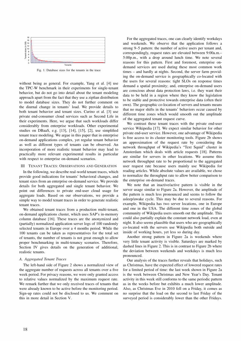
Fig. 1: Database sizes for the tenants in the trace

without being as general. For example, Yang et al. [4] usethe TPC-W benchmark in their experiments for single-tenantbehavior, but do not go into detail about the tenant modelingapproach apart from the fact that they use a zipfian distributionto model database sizes. They do not further comment onthe diurnal change in tenants’ load. We provide details toboth tenant behavior and tenant sizes. Curino et al. [3] useprivate end-consumer cloud services such as Second Life intheir experiments. Here, we argue that such workloads differconsiderably from enterprise workloads. Other experimentalstudies on DBaaS, e.g. [13], [14], [15], [2], use simplifiedtenant trace modeling. We argue in this paper that in enterpriseon-demand applications complex, yet regular tenant behavioras well as different types of tenants can be observed. Anincorporation of more realistic tenant behavior may lead topractically more relevant experimental results in particularwith respect to enterprise on-demand scenarios.

III TENANT TRACES: OBSERVATIONS AND GENERATION

In the following, we describe real-world tenant traces, whichprovide good indications for tenants’ behavioral changes, andtenant sizes from an enterprise on-demand service. We providedetails for both aggregated and single tenant behavior. Wepoint out differences to private end-user cloud usage foraggregate loads. Based on our observations, we provide asimple way to model tenant traces in order to generate realistictenant traces.

We obtained tenant traces from a production multi-tenant,on-demand applications cluster, which uses SAP’s in-memorycolumn database [16]. These traces are the anonymized and(partially) normalized application server logs of 100 randomlyselected tenants in Europe over a 4 months period. While the100 tenants can be taken as representatives for the total setof tenants, the number of tenants is not great enough to allowproper benchmarking in multi-tenancy scenarios. Therefore,Section IV gives details on the generation of additional,realistic tenants.

A. Aggregated Tenant Traces

The left-hand side of Figure 2 shows a normalized view ofthe aggregate number of requests across all tenants over a fiveweek period. For privacy reasons, we were only granted accessto relative values normalized by the maximum request rate.We remark further that we only received traces of tenants thatwere already known to be active before the monitoring period.Sign-up rates could not be disclosed to us. We comment onthis in more detail in Section V.

For the aggregated traces, one can clearly identify workdaysand weekends. We observe that the application follows astrong 9–5 pattern: the number of active users per tenant and,correspondingly, request rates are elevated between 9:00a.m.–5:00p.m., with a drop around lunch time. We note severalreasons for this pattern. First and foremost, enterprise on-demand services are used during these most common worktimes – and hardly at nights. Second, the server farm provid-ing the on-demand service is geographically co-located withthe users for several reasons: tight SLOs on response timesdemand a spatial proximity; and, enterprise on-demand usersare conscious about data protection laws, i.e. they want theirdata to be held in a region where they know the legislationto be stable and protective towards enterprise data (often theirown). The geographic co-location of servers and tenants meansthat no major shifts in the tenants’ behaviors occur caused bydifferent time zones which would smooth out the amplitudeof the aggregated tenant request curve.

We contrast these tenant traces with the private end-userservice Wikipedia [17]. We expect similar behavior for otherprivate end-user service. However, one advantage of Wikipediais free access to its cluster monitoring tools. Figure 2b showsan approximation of the request rate by considering thenetwork throughput of Wikipedia’s “Text Squid” cluster inAmsterdam which deals with article requests [18]. Patternsare similar for servers in other locations. We assume thisnetwork throughput rate to be proportional to the aggregateduser request rate because users mainly use Wikipedia forreading articles. While absolute values are available, we choseto normalize the throughput rate to allow better comparison tothe enterprise on-demand traces.

We note that an inactive/active pattern is visible in theserver usage similar to Figure 2a. However, the amplitude ofthe pattern is much less pronounced and seems to follow theasleep/awake cycle. This may be due to several reasons. Forexample, Wikipedia has two server locations, one in Europeand one in the USA. The different time zones of the globalcommunity of Wikipedia users smooth out the amplitude. Thiscould also partially explain the constant network load, even atnight. It also seems plausible that users who are geographicallyco-located with the servers use Wikipedia both outside andinside of working hours, yet less so during day.

Another strong pattern in Figure 2a is weekends wherevery little tenant activity is visible. Saturdays are marked bydashed lines in Figure 2. This is in contrast to Figure 2b wherethe deviation between weekends and weekdays is much lesspronounced.

Our analysis of the traces further reveals that holidays, suchas Christmas, have the expected effect of lowered request ratesfor a limited period of time: the last week shown in Figure 2ais the week between Christmas and New Year’s Day. Tenantactivity in this week still conforms to the same periodic patternas in the weeks before but exhibits a much lower amplitude.Also, as Christmas Eve in 2010 fell on a Friday, it comes asno surprise that the load on the second to last Friday of thesurveyed period is considerably lower than the other Fridays.

18

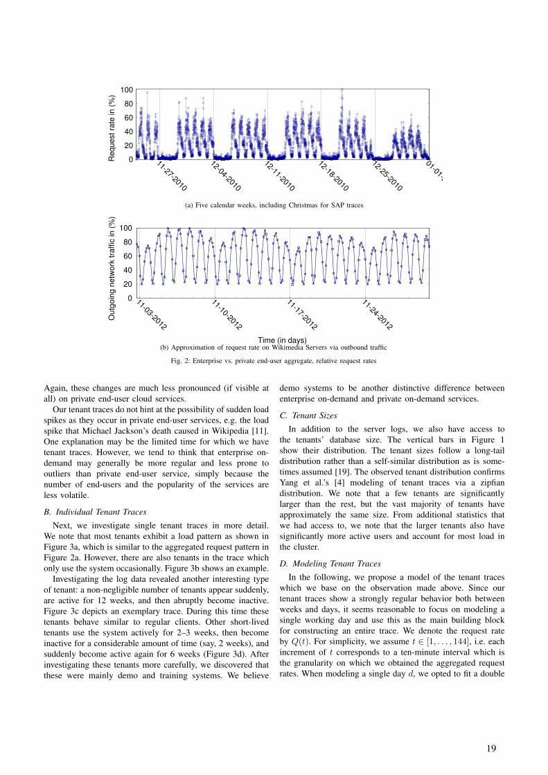
0

20

40

60

80

100

11-27-2010

12-04-2010

12-11-2010

12-18-2010

12-25-2010

01-01-2011

Re

qu

est

rate

in

(%

)

(a) Five calendar weeks, including Christmas for SAP traces

0

20

40

60

80

100

11-03-2012

11-10-2012

11-17-2012

11-24-2012

Ou

tgo

ing

ne

two

rk t

raff

ic in

(%

)

Time (in days)(b) Approximation of request rate on Wikimedia Servers via outbound traffic

Fig. 2: Enterprise vs. private end-user aggregate, relative request rates

Again, these changes are much less pronounced (if visible atall) on private end-user cloud services.

Our tenant traces do not hint at the possibility of sudden loadspikes as they occur in private end-user services, e.g. the loadspike that Michael Jackson’s death caused in Wikipedia [11].One explanation may be the limited time for which we havetenant traces. However, we tend to think that enterprise on-demand may generally be more regular and less prone tooutliers than private end-user service, simply because thenumber of end-users and the popularity of the services areless volatile.

B. Individual Tenant Traces

Next, we investigate single tenant traces in more detail.We note that most tenants exhibit a load pattern as shown inFigure 3a, which is similar to the aggregated request pattern inFigure 2a. However, there are also tenants in the trace whichonly use the system occasionally. Figure 3b shows an example.

Investigating the log data revealed another interesting typeof tenant: a non-negligible number of tenants appear suddenly,are active for 12 weeks, and then abruptly become inactive.Figure 3c depicts an exemplary trace. During this time thesetenants behave similar to regular clients. Other short-livedtenants use the system actively for 2–3 weeks, then becomeinactive for a considerable amount of time (say, 2 weeks), andsuddenly become active again for 6 weeks (Figure 3d). Afterinvestigating these tenants more carefully, we discovered thatthese were mainly demo and training systems. We believe

demo systems to be another distinctive difference betweenenterprise on-demand and private on-demand services.

C. Tenant Sizes

In addition to the server logs, we also have access tothe tenants’ database size. The vertical bars in Figure 1show their distribution. The tenant sizes follow a long-taildistribution rather than a self-similar distribution as is some-times assumed [19]. The observed tenant distribution confirmsYang et al.’s [4] modeling of tenant traces via a zipfiandistribution. We note that a few tenants are significantlylarger than the rest, but the vast majority of tenants haveapproximately the same size. From additional statistics thatwe had access to, we note that the larger tenants also havesignificantly more active users and account for most load inthe cluster.

D. Modeling Tenant Traces

In the following, we propose a model of the tenant traceswhich we base on the observation made above. Since ourtenant traces show a strongly regular behavior both betweenweeks and days, it seems reasonable to focus on modeling asingle working day and use this as the main building blockfor constructing an entire trace. We denote the request rateby Q(t). For simplicity, we assume t ∈ [1, . . . , 144], i.e. eachincrement of t corresponds to a ten-minute interval which isthe granularity on which we obtained the aggregated requestrates. When modeling a single day d, we opted to fit a double

19

0

20

40

60

80

100

cw 48

cw 49

cw 50

cw 51

cw 52

cw 53

cw 54

cw 01

cw 02

cw 03

cw 04

cw 05

cw 06

cw 07

cw 08

cw 09

cw 10

cw 11

cw 12

cw 13

Request ra

te (

%)

Time (calendar weeks)

(a) Regular tenant

0

20

40

60

80

100

cw 48

cw 49

cw 50

cw 51

cw 52

cw 53

cw 54

cw 01

cw 02

cw 03

cw 04

cw 05

cw 06

cw 07

cw 08

cw 09

cw 10

cw 11

cw 12

cw 13

Request ra

te (

%)


(b) Tenant with low activity

0

20

40

60

80

100

cw 48

cw 49

cw 50

cw 51

cw 52

cw 53

cw 54

cw 01

cw 02

cw 03

cw 04

cw 05

cw 06

cw 07

cw 08

cw 09

cw 10

cw 11

cw 12

cw 13

Request ra

te (

%)


(c) Demo system used actively until end of trial

0

20

40

60

80

100

cw 48

cw 49

cw 50

cw 51

cw 52

cw 53

cw 54

cw 01

cw 02

cw 03

cw 04

cw 05

cw 06

cw 07

cw 08

cw 09

cw 10

cw 11

cw 12

cw 13

Request ra

te (

%)


(d) Demo system used only at beginning and end of trial

Fig. 3: Different usage patterns for regular tenants and trial customers

Gaussian function. We use a Gaussian function due to the steepload increases/decreases for beginning and end of workingday. The pronounced lunch-break drop for tenant request ratesaround noon motivates the use of a double Gaussian functionas follows:

Rd(t) = a exp(− (t− µ1)2

2σ21

) + b exp(− (t− µ2)2

2σ22

) + c . (1)

We parametrize (1) such that m(Rd(t) − Qd(t)) is minimal.We denote the mean squared error by m(·). We opted forthe simple model (1) because it fits the typical working dayrhythm with a single lunch break. Future work could includeother functions or more involved versions of (1), e.g. triple,asymmetric Gaussian functions [20].

We randomly chose a work day and fit (1) to it. Figure 4shows the original trace (blue) and the least-squared fittedcurve (green) with mean average absolute error (MAPE) of43% and coefficients

a = 55.06, µ1 = 59.11, σ1 = 8.90,

b = 75.24, µ2 = 88.84, σ2 = 10.64, c = 11.90 .

For modeling a working week w, we suggest shifting Rd(t),i.e.

Rw(t) =∑

t∈[1,144·5]

Rd(t mod 144) ,

adjusting c appropriately. For weekends and public holidaysindicator variables are needed to model the decrease in re-quests. In order to see how well (1) predicts tenant traces,we randomly chose 20 work days and calculated the MAPEbetween the aggregated tenant trace predicted by (1) andthe actual aggregated load. The arithmetic average over the20 MAPEs is 39% which clearly indicates how well (1)generalizes to other work days.

So far, we have modeled the aggregated tenant request rates.We obtain the request rate of a single tenant u by scalingRw(t), i.e. rw,u(t) = sRw(t) by an appropriately chosen s.The distribution of tenant sizes provides a guideline on howto obtain such scale factors s by assuming requests to beproportional to database size. By adding random noise e(t) tothe working day pattern, we can create diversity among equallyscaled tenant traces. We suggest using a normally distributederror, i.e.

e(t) =1

σt√2π

exp(− x2

2σ2t

) . (2)

such that σt = 3 for all t except t ∈ {µi − 5, µi + 5} withi ∈ {1, 2} where σt = 10 better captures the higher volatilityin load. The orange line in Figure 4 shows an example of atenant created by (1) and (2).

For demo tenants, we also rely on Rd(t). Here, a muchsmaller scale factor is appropriate and a variable that indicatesthe limited time window of activity. Similar to regular tenants,adding random noise leads to the desired variety in tenants.

For modeling sizes of tenants, we already remarked thatthey follow a zipfian distribution. We chose to fit

s(u) = a+ bu−c . (3)

We assume that tenants are ordered by size non-increasingly.The position u ∈ [1, . . . , 100] in the sequence of sizescorresponds to the tenant. When we fitted (3), we obtaineda MAPE of 7% for the following parameters

a = 0.015, b = 15.65, c = 0.83 . (4)

The red line in Figure 1 shows (3) with parameters (4).

Having discussed how to generate tenant traces syntheticallybased on our observations, we consider the case that onehas access to a limited number of tenant traces and needsto generate more tenant traces.

20

0

20

40

60

80

100

0:001:00

2:003:00

4:005:00

6:007:00

8:009:00

10:00

11:00

12:00

13:00

14:00

15:00

16:00

17:00

18:00

19:00

20:00

21:00

22:00

23:00

24:00

Re

qu

est

rate

in

(%

)

Fit plus Normal Noise Fit Real Data

Fig. 4: Aggregated vs Generated Request Rates

IV BOOTSTRAPPING

As mentioned in Section I, it is difficult to obtain real-worldtenant traces. While the previous chapter dealt with modelingtenant traces, we consider enlarging a set of given tenant tracesin the following. We provide a straight-forward bootstrappingmethodology with a single parameter, the bootstrap windowsize. For our use case, we show how to identify an appropriatevalue for this parameter.

In the server logs we obtained, a tenant trace comprises therequest rates of a tenant across a 4-month-period aggregated inten-minute intervals. We refer to a point in discretized time,such as the ten-minute interval in our case, as a tick in thetenant trace.

We were only granted access to a subset of the traces, 100tenants in total. However, this random sample gives a realisticimpression of the overall customer base. Unfortunately, thesample is not large enough to conduct meaningful experimentswith realistically-sized server farms. For example, in October2007, the SaaS CRM vendor RightNow had 3000 tenantsdistributed across 400 MySQL database instances [21]. Tosimulate a realistically sized DBaaS scenario, it is thereforenecessary to increase the pool of tenant traces. Here, wesuggest bootstrapping in order to enlarge the set of tenanttraces such that◦ the trace of a bootstrapped tenant shows the temporal

characteristics of a working week,◦ during a loaded workday, an active server holds 1–100

tenants,◦ each tenant has a realistic size and trace volume, and,◦ bootstrapped tenants resemble the sample tenants while

being sufficiently distinct from them and each other.In our methodology we follow [22]. Our methodology cannaturally be combined with the generation of tenant traces asshown in the previous section. This may be interesting forexample in the case where certain work day patterns are notpresent in the traces.

A. Bootstrapping Process

Our bootstrapping process produces for each original ten-ant trace, which we call a parent trace, a fixed number cof child traces. Figure 5 shows a schematic overview ofthe bootstrapping process. Apart from deciding on the trace

pattern, we also need to assign a size to the child tenant.Based on our observations in Section III, we differentiatebetween regular tenants and demo tenants. Regular tenantsall have comparably similar request rate patterns but highlyvarying sizes. Demo tenants have irregular usage patterns butexhibit smaller difference in their sizes. Therefore, it seemsreasonable to choose size independently of trace pattern forregular tenants.

In more detail, our bootstrapping works as follows. Fromeach parent tenant trace, we create c child tenants. The numberof bootstrap copies c is a parameter of the process which wecan choose. Each child tenant is then given a size drawn atrandom from a list of all parent tenant sizes (depending onthe parent tenant being a demo or a regular tenant).

The process of bootstrapping a parent trace into a singlechild trace, shown in Figure 5, is as follows:1) The parent trace is divided into equally sized subintervals

of size W with the last subinterval of the trace potentiallyhaving size less than W . We call a subinterval a windowin the following.

2) The indices of a window of the parent trace corresponddirectly to the indices of a window in the child trace.Window i spans {iW, iW + 1, . . . , iW +W − 1} in bothparent and child traces.

3) For each parent window, W values are chosen at randomwith replacement and uniform probability. These values areplaced into the corresponding child window in the orderthat they are chosen.

The quality of the bootstrapping processing depends on thechoice of W . Section IV-B provides details.

The bootstrapping process results in c times many newtenants, each with a realistic size and a trace that is similarbut not identical to its parent. For 100 parent tenant traces, wehave 100 · c many tenants. By drawing the child tenant size atrandom from all parent tenant sizes, we doubly ensure that thechild is not too similar to its parent as size and request rateinfluence the load that a tenant puts onto a DBaaS cluster [10].

B. Choosing the bootstrap window size

In the following, we describe how to obtain a good value forW which determines the similarity between child and parenttenant. For a choice of a small W , we run the risk of all or most

21

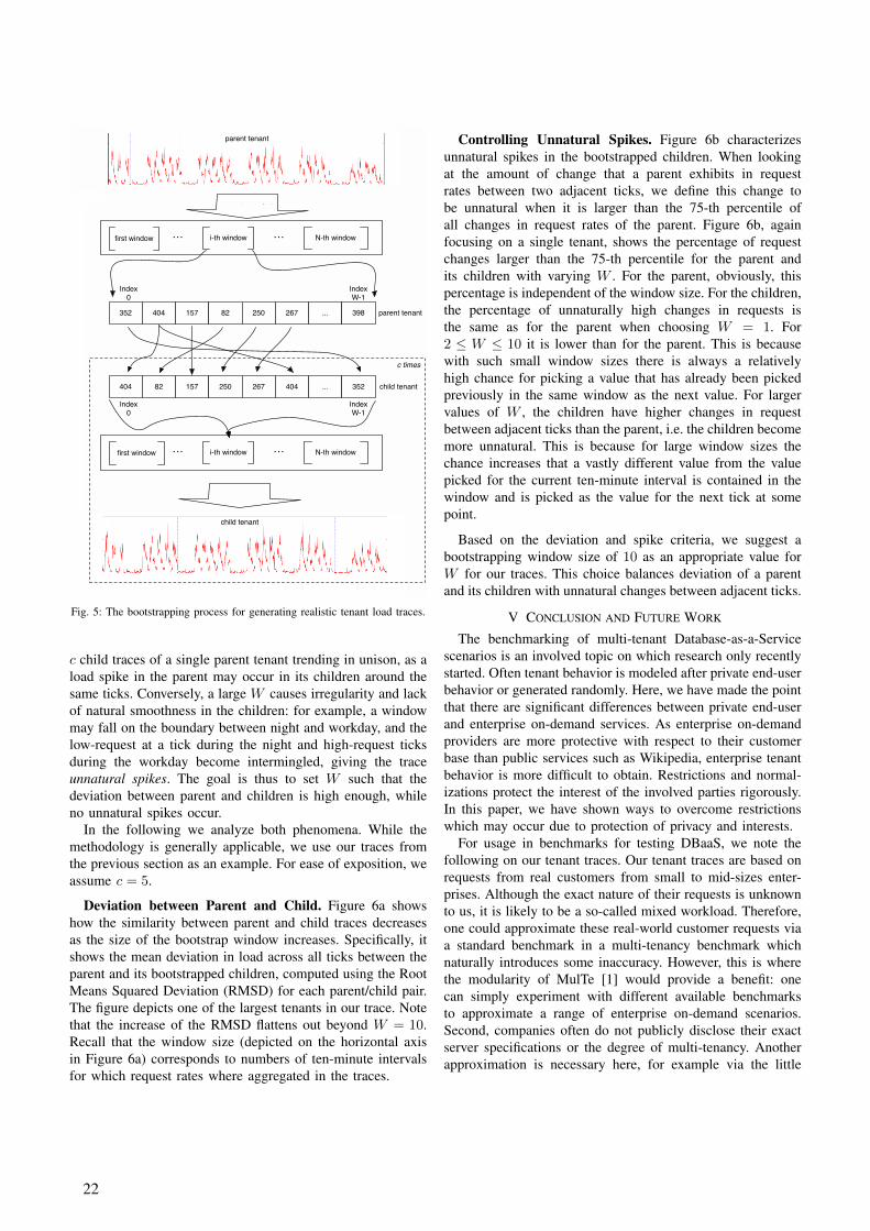
first window i-th window N-th window… …

352 404 157 82 250 267 ... 398

404 82 157 250 267 404 ... 352

Index0

IndexW-1

IndexW-1

Index0

first window i-th window N-th window… …

child tenant

parent tenant

c times

parent tenant

child tenant

Fig. 5: The bootstrapping process for generating realistic tenant load traces.

c child traces of a single parent tenant trending in unison, as aload spike in the parent may occur in its children around thesame ticks. Conversely, a large W causes irregularity and lackof natural smoothness in the children: for example, a windowmay fall on the boundary between night and workday, and thelow-request at a tick during the night and high-request ticksduring the workday become intermingled, giving the traceunnatural spikes. The goal is thus to set W such that thedeviation between parent and children is high enough, whileno unnatural spikes occur.

In the following we analyze both phenomena. While themethodology is generally applicable, we use our traces fromthe previous section as an example. For ease of exposition, weassume c = 5.

Deviation between Parent and Child. Figure 6a showshow the similarity between parent and child traces decreasesas the size of the bootstrap window increases. Specifically, itshows the mean deviation in load across all ticks between theparent and its bootstrapped children, computed using the RootMeans Squared Deviation (RMSD) for each parent/child pair.The figure depicts one of the largest tenants in our trace. Notethat the increase of the RMSD flattens out beyond W = 10.Recall that the window size (depicted on the horizontal axisin Figure 6a) corresponds to numbers of ten-minute intervalsfor which request rates where aggregated in the traces.

Controlling Unnatural Spikes. Figure 6b characterizesunnatural spikes in the bootstrapped children. When lookingat the amount of change that a parent exhibits in requestrates between two adjacent ticks, we define this change tobe unnatural when it is larger than the 75-th percentile ofall changes in request rates of the parent. Figure 6b, againfocusing on a single tenant, shows the percentage of requestchanges larger than the 75-th percentile for the parent andits children with varying W . For the parent, obviously, thispercentage is independent of the window size. For the children,the percentage of unnaturally high changes in requests isthe same as for the parent when choosing W = 1. For2 ≤ W ≤ 10 it is lower than for the parent. This is becausewith such small window sizes there is always a relativelyhigh chance for picking a value that has already been pickedpreviously in the same window as the next value. For largervalues of W , the children have higher changes in requestbetween adjacent ticks than the parent, i.e. the children becomemore unnatural. This is because for large window sizes thechance increases that a vastly different value from the valuepicked for the current ten-minute interval is contained in thewindow and is picked as the value for the next tick at somepoint.

Based on the deviation and spike criteria, we suggest abootstrapping window size of 10 as an appropriate value forW for our traces. This choice balances deviation of a parentand its children with unnatural changes between adjacent ticks.

V CONCLUSION AND FUTURE WORK

The benchmarking of multi-tenant Database-as-a-Servicescenarios is an involved topic on which research only recentlystarted. Often tenant behavior is modeled after private end-userbehavior or generated randomly. Here, we have made the pointthat there are significant differences between private end-userand enterprise on-demand services. As enterprise on-demandproviders are more protective with respect to their customerbase than public services such as Wikipedia, enterprise tenantbehavior is more difficult to obtain. Restrictions and normal-izations protect the interest of the involved parties rigorously.In this paper, we have shown ways to overcome restrictionswhich may occur due to protection of privacy and interests.

For usage in benchmarks for testing DBaaS, we note thefollowing on our tenant traces. Our tenant traces are based onrequests from real customers from small to mid-sizes enter-prises. Although the exact nature of their requests is unknownto us, it is likely to be a so-called mixed workload. Therefore,one could approximate these real-world customer requests viaa standard benchmark in a multi-tenancy benchmark whichnaturally introduces some inaccuracy. However, this is wherethe modularity of MulTe [1] would provide a benefit: onecan simply experiment with different available benchmarksto approximate a range of enterprise on-demand scenarios.Second, companies often do not publicly disclose their exactserver specifications or the degree of multi-tenancy. Anotherapproximation is necessary here, for example via the little

22

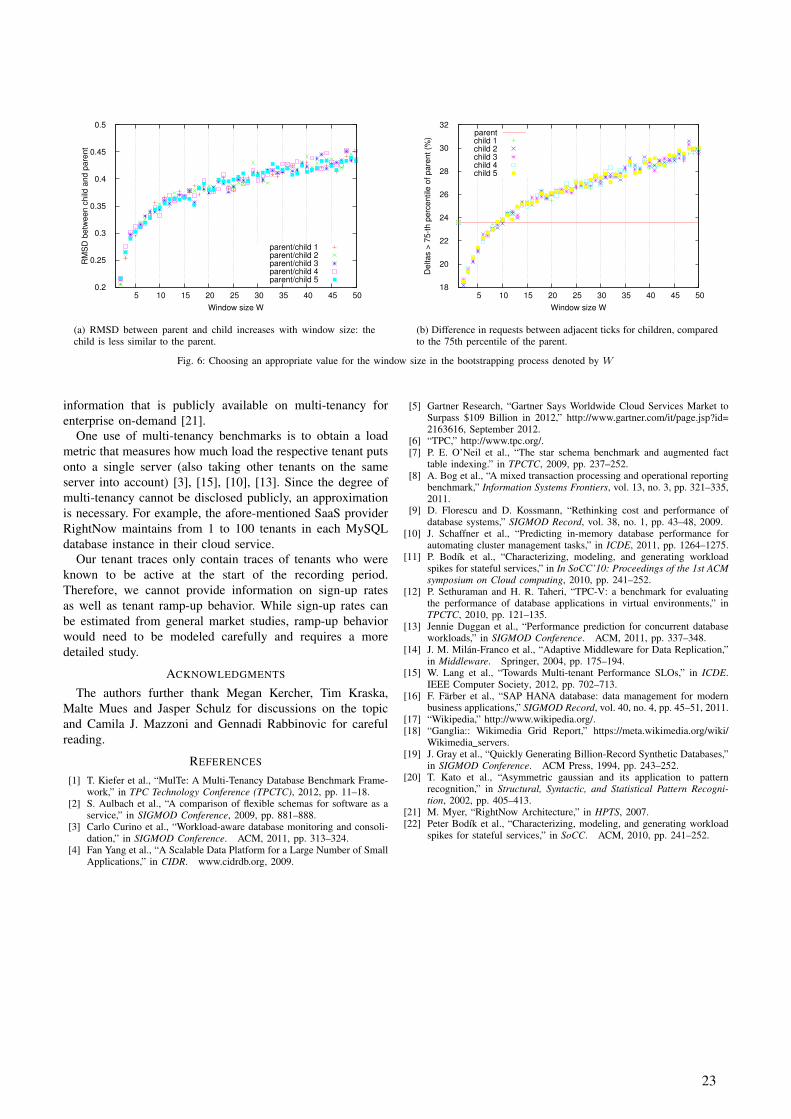
0.2

0.25

0.3

0.35

0.4

0.45

0.5

5 10 15 20 25 30 35 40 45 50

RM

SD

betw

een c

hild

and p

are

nt

Window size W

parent/child 1parent/child 2parent/child 3parent/child 4parent/child 5

(a) RMSD between parent and child increases with window size: thechild is less similar to the parent.

18

20

22

24

26

28

30

32

5 10 15 20 25 30 35 40 45 50

Deltas >

75-t

h p

erc

entile

of pare

nt (%

)

Window size W

parentchild 1child 2child 3child 4child 5

(b) Difference in requests between adjacent ticks for children, comparedto the 75th percentile of the parent.

Fig. 6: Choosing an appropriate value for the window size in the bootstrapping process denoted by W

information that is publicly available on multi-tenancy forenterprise on-demand [21].

One use of multi-tenancy benchmarks is to obtain a loadmetric that measures how much load the respective tenant putsonto a single server (also taking other tenants on the sameserver into account) [3], [15], [10], [13]. Since the degree ofmulti-tenancy cannot be disclosed publicly, an approximationis necessary. For example, the afore-mentioned SaaS providerRightNow maintains from 1 to 100 tenants in each MySQLdatabase instance in their cloud service.

Our tenant traces only contain traces of tenants who wereknown to be active at the start of the recording period.Therefore, we cannot provide information on sign-up ratesas well as tenant ramp-up behavior. While sign-up rates canbe estimated from general market studies, ramp-up behaviorwould need to be modeled carefully and requires a moredetailed study.

ACKNOWLEDGMENTS

The authors further thank Megan Kercher, Tim Kraska,Malte Mues and Jasper Schulz for discussions on the topicand Camila J. Mazzoni and Gennadi Rabbinovic for carefulreading.

REFERENCES

[1] T. Kiefer et al., “MulTe: A Multi-Tenancy Database Benchmark Frame-work,” in TPC Technology Conference (TPCTC), 2012, pp. 11–18.

[2] S. Aulbach et al., “A comparison of flexible schemas for software as aservice,” in SIGMOD Conference, 2009, pp. 881–888.

[3] Carlo Curino et al., “Workload-aware database monitoring and consoli-dation,” in SIGMOD Conference. ACM, 2011, pp. 313–324.

[4] Fan Yang et al., “A Scalable Data Platform for a Large Number of SmallApplications,” in CIDR. www.cidrdb.org, 2009.

[5] Gartner Research, “Gartner Says Worldwide Cloud Services Market toSurpass $109 Billion in 2012,” http://www.gartner.com/it/page.jsp?id=2163616, September 2012.

[6] “TPC,” http://www.tpc.org/.[7] P. E. O’Neil et al., “The star schema benchmark and augmented fact

table indexing.” in TPCTC, 2009, pp. 237–252.[8] A. Bog et al., “A mixed transaction processing and operational reporting

benchmark,” Information Systems Frontiers, vol. 13, no. 3, pp. 321–335,2011.

[9] D. Florescu and D. Kossmann, “Rethinking cost and performance ofdatabase systems,” SIGMOD Record, vol. 38, no. 1, pp. 43–48, 2009.

[10] J. Schaffner et al., “Predicting in-memory database performance forautomating cluster management tasks,” in ICDE, 2011, pp. 1264–1275.

[11] P. Bodık et al., “Characterizing, modeling, and generating workloadspikes for stateful services,” in In SoCC’10: Proceedings of the 1st ACMsymposium on Cloud computing, 2010, pp. 241–252.

[12] P. Sethuraman and H. R. Taheri, “TPC-V: a benchmark for evaluatingthe performance of database applications in virtual environments,” inTPCTC, 2010, pp. 121–135.

[13] Jennie Duggan et al., “Performance prediction for concurrent databaseworkloads,” in SIGMOD Conference. ACM, 2011, pp. 337–348.

[14] J. M. Milan-Franco et al., “Adaptive Middleware for Data Replication,”in Middleware. Springer, 2004, pp. 175–194.

[15] W. Lang et al., “Towards Multi-tenant Performance SLOs,” in ICDE.IEEE Computer Society, 2012, pp. 702–713.

[16] F. Farber et al., “SAP HANA database: data management for modernbusiness applications,” SIGMOD Record, vol. 40, no. 4, pp. 45–51, 2011.

[17] “Wikipedia,” http://www.wikipedia.org/.[18] “Ganglia:: Wikimedia Grid Report,” https://meta.wikimedia.org/wiki/

Wikimedia servers.[19] J. Gray et al., “Quickly Generating Billion-Record Synthetic Databases,”

in SIGMOD Conference. ACM Press, 1994, pp. 243–252.[20] T. Kato et al., “Asymmetric gaussian and its application to pattern

recognition,” in Structural, Syntactic, and Statistical Pattern Recogni-tion, 2002, pp. 405–413.

[21] M. Myer, “RightNow Architecture,” in HPTS, 2007.[22] Peter Bodık et al., “Characterizing, modeling, and generating workload

spikes for stateful services,” in SoCC. ACM, 2010, pp. 241–252.

23

Quasi-Real Time Individual Customer Based Forecasting of Energy LoadDemand Using In Memory Computing

– Project Report –

Witold Abramowicz Monika Kaczmarek Tomasz RudnyWioletta Sokolowska

Department of Information SystemsFaculty of Informatics and Electronic Economy

Poznan University of EconomicsAl. Niepodleglosci 10, 61-875 Poznan

[email protected]

Abstract

This report presents the individual customer based ap-proach to energy demand forecasting using the compu-tational power of SAP HANA. The research hypothesiswas that demand forecasting can be done in quasi-realtime, even if conforming to bottom-up approach, i.e.,computing separate forecasts for each customer. Thereport provides information on the project idea, usedHPI Future SOC Lab resources, findings as well asnext steps envisioned.

1 Introduction

The European energy markets are facing many chal-lenges – e.g., usage of renewable energy sources, ap-plication of smart metering and, consequently, the emergence of new players in the market (e.g., of pro-sumers). However, one of the biggest challenges the energy sector still needs to address, is how to accu-rately predict a short- and long-term value of energy demand, as well as the level of energy production from different sources. Erroneous forecasts entail costs, resulting, among others, from the need to purchase the additional energy capacity at the energy balanc-ing market for a significantly higher price. In turn, the excess capacity in the system entails incurring fixed costs, resulting from the maintenance of overcapacity. In our project, we focused on a short term prognosis of energy demand. Taking into account a large num-ber of influence factors and their uncertainty, ”it is not possible to design an exact physical model for the en-ergy demand” [4]. Therefore, usually both the long term and short term energy demand is calculated us-ing statistical models (e.g., regression models, proba-bilistic models [7, 6, 3]), artificial intelligence tools

(e.g., [8]) or hybrid approaches (e.g., [2, 5]). They all try to describe the influence of climate factors, op-erating conditions [4] and other variables, on the en-ergy consumption. The quality of the demand forecast methods depends first of all, on the availability of his-torical consumption data, as well as on the knowledge on the important influence variables and their values. The second factor is the application of an appropriate forecast tool and method taking into account the data that we have, as well as existing limitations (e.g., com-putational).

Most of the existing approaches to energy demand prognosis focuses on characterising aggregated elec-tricity system demand load profile. However, as shown by many researchers and practitioners, the energy load forecasting can be done more accurately, if forecasts are calculated for all customers separately and then combined via bottom-up strategy to produce the total load forecast [1, 3]. The reason for it is that the char-acteristics of aggregated and individual profiles are different (e.g., they have different shapes - the individ-ual profiles show peaks in the morning and evenings and their shapes vary for different days of the week and part of the year). In fact, the individual electric-ity load profile is influenced by the number of factors, which may be divided in the following categories [3]: electricity demand variations between customers, sea-sonal electricity demand effects, intra-daily variations, and diurnal variations in electricity demand.

Also, additional improvement is expected, if differentmodels and parameters can be tested quickly to pro-vide the best model selection capability. Quasi realtime load forecasting could lead to substantial savingsfor companies and also for the environment, up tillnow however, it was computationally difficult, as for atypical energy seller a number of residential customersexceeds hundreds of thousands.

25

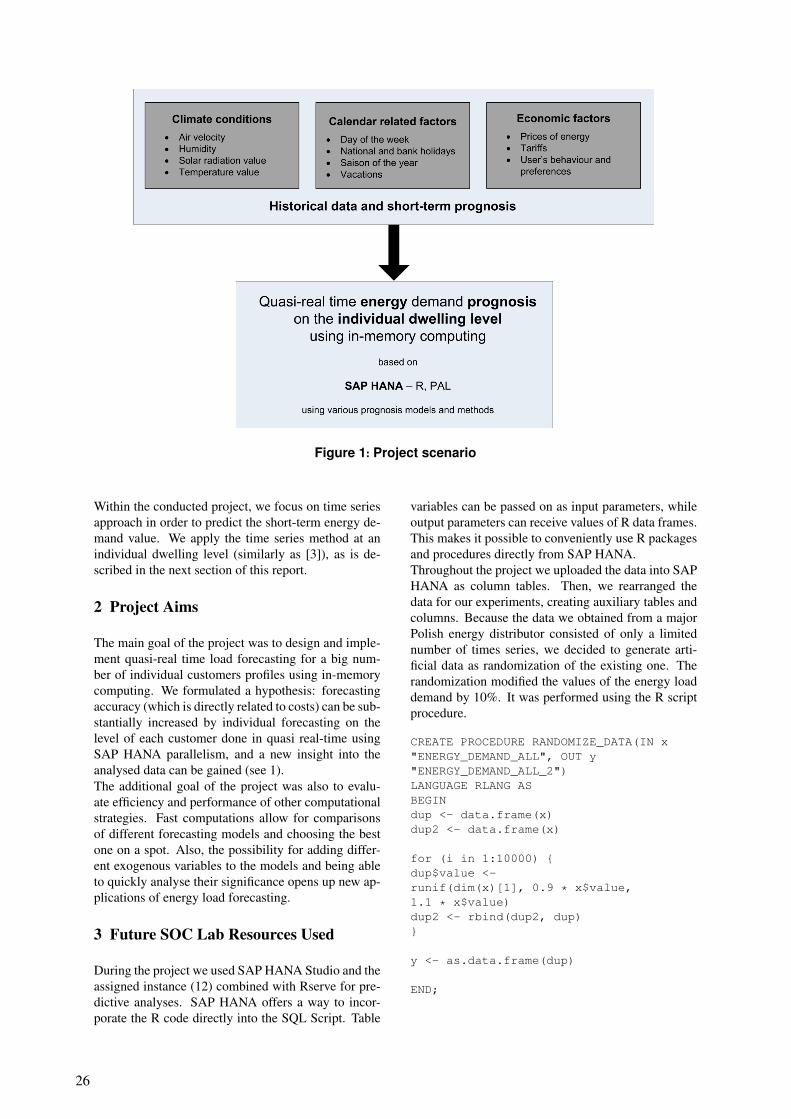
Figure 1: Project scenario

Within the conducted project, we focus on time seriesapproach in order to predict the short-term energy de-mand value. We apply the time series method at anindividual dwelling level (similarly as [3]), as is de-scribed in the next section of this report.

2 Project Aims

The main goal of the project was to design and imple-ment quasi-real time load forecasting for a big num-ber of individual customers profiles using in-memorycomputing. We formulated a hypothesis: forecastingaccuracy (which is directly related to costs) can be sub-stantially increased by individual forecasting on thelevel of each customer done in quasi real-time usingSAP HANA parallelism, and a new insight into theanalysed data can be gained (see 1).The additional goal of the project was also to evalu-ate efficiency and performance of other computationalstrategies. Fast computations allow for comparisonsof different forecasting models and choosing the bestone on a spot. Also, the possibility for adding differ-ent exogenous variables to the models and being ableto quickly analyse their significance opens up new ap-plications of energy load forecasting.

3 Future SOC Lab Resources Used

During the project we used SAP HANA Studio and theassigned instance (12) combined with Rserve for pre-dictive analyses. SAP HANA offers a way to incor-porate the R code directly into the SQL Script. Table

variables can be passed on as input parameters, whileoutput parameters can receive values of R data frames.This makes it possible to conveniently use R packagesand procedures directly from SAP HANA.Throughout the project we uploaded the data into SAPHANA as column tables. Then, we rearranged thedata for our experiments, creating auxiliary tables andcolumns. Because the data we obtained from a majorPolish energy distributor consisted of only a limitednumber of times series, we decided to generate arti-ficial data as randomization of the existing one. Therandomization modified the values of the energy loaddemand by 10%. It was performed using the R scriptprocedure.

CREATE PROCEDURE RANDOMIZE_DATA(IN x"ENERGY_DEMAND_ALL", OUT y"ENERGY_DEMAND_ALL_2")LANGUAGE RLANG ASBEGINdup <- data.frame(x)dup2 <- data.frame(x)

for (i in 1:10000) {dup$value <-runif(dim(x)[1], 0.9 * x$value,1.1 * x$value)dup2 <- rbind(dup2, dup)}

y <- as.data.frame(dup)

END;

26

Figure 2: Prognosis error comparison - individual level and total level

combined with R service we used the new efficientPredictive Analysis Library (PAL), however, we didnot yet run the same experiments on PAL.The following experiments were run on SAP HANAusing the aforementioned resources:

• Computing the summary forecast by summing allindividual time series and calculating the (single)forecast over the summarized data,

• Calculating individual forecasts for all customers,then summarizing the forecasted values to com-pute the summary forecast,

• Comparing the forecasting error between differ-ent scenarios,

• Comparing different forecasting models - amongothers Holt-Winters exponential smoothing andARIMA.

The experiments conducted so far focused on evaluat-ing SAP HANA capabilities for time series forecast-ing, data manipulation and storage, as well as organiz-ing the code.We also had to impute the data as sometimes the valueof the historical energy load demand was missing. Theimputation code is presented below:

CREATE PROCEDURE IMPUTE_MISSING(IN x"totals",OUT y "totals_imputed")LANGUAGE RLANG AS BEGINmissing <- is.na(x$value)n.missing <- sum(missing)x.obs <- x$value[!missing]imputed <- ximputed$value[missing] <-sample(x.obs, n.missing, replace=TRUE)y <- as.data.frame(imputed)END;

4 Findings

As stated in the project proposal our aim is to evalu-ate SAP HANA capabilities in the area of fast massivetime series computations. To this end we implemented

a set of R procedures. The performed experimentsproved that SAP HANA is an efficient tool due toits in-memory paradigm as well as parallel processingpower. We were able to generate forecasts using vari-ous models based on a 180 days historical data with a14 days horizon. The models tested included ARIMAand Holt-Winters exponential smoothing. The resultsshow that SAP HANA can be efficiently used for thispurpose.The runtime for calculating summary forecast usingthe bottom-up approach varies around 600 ms asshown on the histogram (see fig. 2). It is not onlypossible calculate summary forecast in quasi-real time,but also to run different models and choose the best fit-ted one for each customer.The code for forecasting can be nicely and neatly writ-ten in R as shown on the example of Holt-Winters ex-ponential smoothing:

CREATE PROCEDURE FS_STEP(IN x "input2",IN temp "temp", OUT y "totals_forecast")LANGUAGE RLANG ASBEGINts1 <- ts(x$value, frequency=24)m <- HoltWinters(ts1)f <- predict(m, n.ahead=14*24)

forecast <- f[1:14*24]

Figure 3: Runtime histogram of simple forecasting via bottom-up aproach

Apart from the standard installation of SAP HANA

27

y <- as.data.frame(cbind(temp, forecast))END;

Our proposed approach needs further works and pol-ishing, but the initial hypothesis has been partiallyproven - SAP HANA is an efficient tool for energymarket and time series forecasting (see fig. 3). How-ever, the learning curve proved to be slightly steep,as mastering different specific details of SAP HANAscripting may not be easy.Some of the obstacles we encountered included:

• problems with column store order of tables whenmanipulating data within SQL script procedures,

• problems with passing out data frames from Rback to SAP HANA,

• problems with loop variables in SQL script.

We are convinced that these early problems can beovercome and this does not in any way diminish thevalue of SAP HANA. However, it was the lesson wehad to learn.

5 Next Steps

The already conducted research using the Future SOCLab resources allowed us to gain some insight intoSAP HANA and the prognosis challenge and provedthe benefits from the application of the in-memorycomputing offered by HANA. However, 5 months pe-riod turned out to be not enough time to test all our hy-potheses and conduct all of the planned experiments.What we would like to do as next steps includes:

• building regression models to identify impact ofexogenous variables,

• implement an automatic procedures to run all thetests and experiments,

• simulate special events as it is known that theyshould worsen to top-down forecast, while not af-fecting bottom-up approach,

• write selected algorithms in C langauge andlaunch them on the available NVidia box.

In addition, we started a collaboration with the localenergy provider regarding the forecasting of the en-ergy production from renewable sources. As we wereable to obtain relevant data on energy generation, inaddition, we would like to conduct research and runexperiments to prove that SAP HANA and in-memorycomputing can be applied in this area as well.

References

[1] W. Charytoniuk, M.-S. S. Chen, P. Kotas, andP. Van Olinda. Demand forecasting in power distri-bution systems using nonparametric probability den-sity estimation. Power Systems, IEEE Transactions,14/4:1200–1206, 1999.

[2] M. S. Kiran, E. Ozceylan, M. Gunduz, and T. Paksoy.A novel hybrid approach based on particle swarm opti-mization and ant colony algorithm to forecast energydemand of turkey. Energy Conversion and Manage-ment, 53(1):75 – 83, 2012.

[3] F. McLoughlin, A. Duffy, and M. Conlon. Evaluationof time series techniques to characterise domestic elec-tricity demand. Energy, 50(0):120 – 130, 2013.

[4] W. Schellong. Energy Management Systems, chapterEnergy Demand Analysis and Forecast, pages 101–120.InTech, 2011.

[5] R. Shakouri, G.H.and Nadimi and F. Ghaderi. A hybridtsk-fr model to study short-term variations of the elec-tricity demand versus the temperature changes. ExpertSystems with Applications, 36(2, Part 1):1765 – 1772,2009.

[6] C. Wang, G. Grozev, and S. Seo. Decomposition andstatistical analysis for regional electricity demand fore-casting. Energy, 41(1):313 – 325, 2012. ¡ce:title¿23rdInternational Conference on Efficiency, Cost, Optimiza-tion, Simulation and Environmental Impact of EnergySystems, ECOS 2010¡/ce:title¿.

[7] J. Wang, X. Ma, J. Wu, and Y. Dong. Optimizationmodels based on gm (1) and seasonal fluctuation forelectricity demand forecasting. International Journal ofElectrical Power & Energy Systems, 43(1):109 – 117,2012.

[8] M. Zadeh, S. and A. Masoumi. Modeling residentialelectricity demand using neural network and economet-rics approaches. In International Conference on Com-puters and Industrial Engineering (CIE), 2010 40th,pages 1 –6, july 2010.

28

A framework for comparing the performance of in-memory and traditional disk-based databases

Vassilena Banova Technische Universität München

Chair for Information Systems Boltzmannstr. 3, 85748 Garching, Germany

[email protected]

Alexandru Danciu Technische Universität München


[email protected]

Helmut Krcmar Technische Universität München


[email protected]

Abstract

Enterprises are facing an increasing amount of data, and rely more than ever on flexible and fast methods of data analysis. A proposed solution is the switch to in-memory database systems which promise huge performance increases. Unfortunately recent litera-ture does not provide performance comparisons of main-memory and classical storage based database systems in enterprise use cases. A literature review is conducted identifying the scenario of discovering frequent item-sets as an appropriate use case to perform such a comparison. Requirements on a test environment are provided and a tool supporting those tests is implemented, encouraging the execution of OLAP, OLTP and mixed workload test-suites.

1 Introduction

Today’s enterprises store and collect more data than ever. It is estimated that the fortune 500 enterprises store approximately seven to ten years of customer data [1]. This amount is told to increase even further in the coming years [2]. Amongst others this data is used in the context of Business Intelligence & Ana-lytics“(BI&A) to gain insights on the market and make critical decisions in a timely manner based on up to date information [3]. But the huge amount of data makes it necessary to narrow the data down or to work with pre-calculated results what limits the flex-ibility and expressiveness of the analysis [4]. In an environment of fast changing market conditions and customer wishes this flexibility is crucial to recog-nize influences on the own business and react on undesirable developments [2].

A frequently used term in this context is “Big Data” what describes the processing and analysis of huge amounts of data with complex structure [3] and is sometimes referred to as a scaled BI&A [5]. The properties of Big Data, “high-volume, high-variety, high-velocity, and high-veracity“ [6], often referred to as the three “HVs” [6], make it necessary for enter-prises to come up with new requirements on storage, management, analysis and visualization of data [3]. One proposed solution to deal with this requirements is the use of in-memory databases, which describe database systems holding the entire dataset in main memory [7]. A study conducted amongst German IT-professionals in 2012, pointed out that every fifth enterprise thinks that meeting the challenges of the future data volume is only possible using in-memory technology. But the same study pointed out, that 60% of the enterprises are not able to make a clear deci-sion on whether in-memory databases are relevant to them. They are especially concerned whether the proposed advantages of in-memory technology can really be leveraged in their enterprise [2]. To achieve a better understanding about the effects of in-memory databases and to be able to make a found decision on whether to invest into in-memory tech-nology and migrate from traditional disk-based stor-age to main memory storage enterprises need tests to be executed, comparing those technologies in enter-prise use case scenarios and providing insights on basic characteristics of the database systems. Those tests will help enterprises to determine the most suit-able set up for their needs. This project aims on de-veloping some basic test cases and the necessary toolset for executing this kind of tests.

29

2 Project Implementation

2.1 Project Description The project aims at the development of a testing environment for the comparison of response times of in-memory based and classical disk storage databases in enterprise use case scenarios. Two identical virtual machines, one with an in-memory database system, the other with a classical disk based storage database are used to verify, that the developed test cases can be executed on such environments. Therefore the same dataset is deployed to both virtual machines. Queries are generated and executed from a third, independent source where response time is measured, too. The target is to pro-vide a test setup including enterprise use case scenar-ios being able to compare two database systems.

2.2 Project Phases In a first phase a literature review on database per-formance and benchmarks was conducted to identify relevant stakeholders, use case scenarios and re-quirements for testing. During this literature review four major groups of stakeholders and their major topics of interest could be identified. The four groups, consisting of database developers, database administrators, business analysts and end-user/deci-sion makers were characterized and the assumption was made, that the group of business analysts is the most appropriate target group and that scenarios in data mining such as the identification of frequent item-sets or the measurement of profits and losses generated by a specific sales-channel and its compo-nents are appropriate use case scenarios for testing. Furthermore the absence of tests comparing an in-memory database to a classical disk storage database in a comprehensible, reproducible way and on equal conditions could be approved. In a second phase a framework for plan execution was developed simulating different circumstances for the virtual machines. The framework focuses on varying three components in the test environment - namely the number of threads executing one query in parallel, the size of the dataset and plans of execu-tion, determining whether update and select state-ments are executed irrespective of each other or not. The number of threads and the different datasets represent the different amount of users and size of an enterprise. Different plans of execution allow a com-parison of the databases for different areas of applica-tion. This increases the expandability of the tool to further application domains and aims on evaluating performance in mixed OLTP (Online Transaction Processing) and OLAP (Online analytical Pro-cessing) workloads. In a third phase appropriate datasets were generated and queries for testing were developed. Furthermore a tool was implemented to execute the tests and

measure response time on both virtual machines on equal conditions. Data is extracted from the publicly available data generator of the TPC-DS benchmark, an industry standard benchmark for decision support systems (see: www.tpc.org), as it is available for free and approved to provide appropriate data for performance testing. For reasons of simplification only two of those tables were used. “catalog_sales” and “cata-log_returns” which provide a fact table of sales through the catalog sales channel including items and orders and the profit and loss information of each line item. This information, in combination with the page number of the catalog, the item was ordered from, allows to execute the afore mentioned business use case scenarios. The tool for query execution is writ-ten in Java and uses JDBC to send the chosen queries to the databases and measure their response time.

3 Description of the Virtual Machines

The virtual machines provided by the HPI Future SOC Lab both had 64 GB main memory, a hard drive disk with a capacity of 100GB and a total of eight CPUs available. They are both located in the same network and run a Linux Kernel 2.6.32.59-0.7.

4 Test-framework and Toolset

4.1 Requirements The test-framework is supposed to provide decision support for enterprises when deciding on switching to or adding an in-memory database to their IT land-scape. Therefore the framework for testing has to simulate several environmental scenarios/enterprise characteristics and provide details about the influ-ences on performance if those environmental factors change. As a test environment will never exactly match a real enterprise, metrics of comparison should be expressed in relative numbers and an easy, com-prehensible way such as “On a level playing field, an increase of users by factor x performance loss of system A is factor z and performance loss of system B is factor y - B runs r times faster than A”. Another important factor for generating an as equal as possible setup of the two databases, is to forbid every kind of tuning, such as additional indexes. Methods or elementary approaches as parts of the database management system can be used. Therefore tuning mechanisms such as adding further indexes to a table have to be avoided. Using a columnar table layout is appropriate. Basically the databases are supposed to be used in out-of-the-box versions as extra tuning might not be available for both database instances the same way and the test is not supposed to compare different tuning mechanisms. Queries are supposed to be expressed in a way, that both database systems can handle the same expres-

30

sion as good as possible. Furthermore the queries have to be repeatable and comprehensible and have to be logged or generated in a way that reproduction is explicit. The combination of queries and workload should try to emphasize the differences in the database systems and should therefore be designed to point out strengths and weaknesses of both instances. The measurement of response time may not include the time necessary for query generation or the writing of result-sets. Therefore the machine running the test tool shall not be changed during tests and only the execution time of the SQL Statement is to be meas-ured.

4.2 Design of tests Environmental Factors To meet the above mentioned requirements for simu-lating environmental factors the Queries are supposed to be executed by {1, 5, 10, 20, 40} Threads in paral-lel on a catalog_sales table of sizes {5GB, 10GB, 20GB, 40GB, 60GB, 80GB}. Those values were chosen as they can be computed in a relatively mod-erate time and are based on almost constant growth-rate. The high volumes of data are selected as they are close to (60GB) or even above (80GB) the avail-able main memory (64GB). Additionally to the catalog_sales table the cata-log_returns table is used with a constant size of 0.5 GB. Queries One test consists of six queries which can be grouped into three categories. The first category consists of queries which perform very basic and simple SQL statements like selects or unions. The second group of queries are either inserting lines or updating tables and therefore represent OLTP workload. The third group includes rather expensive queries including joins and calculations. It has to be mentioned, that the queries are not de-signed to perform their tasks in the most efficient way, but to generate workload on the database. The six queries are: - Insert lines: a specified number of Lines {1, 50,

100, 150, 200, 250} is inserted into the catalog sales table at once. This query was chosen to evaluate the write performance for a high num-ber of columns.

- Update one: This query updates one column in the catalog_sales table for a specific collection of items. This helps to evaluate update performance of single column and creates OLTP workload.

- Update six: This query updates six different columns of the catalog sales table for a prede-fined set of items. Here the update performance of multiple columns is tested.

- Select all: this statement simply returns the whole catalog_sales table and gives insight about the read performance of multiple columns.

- Select distinct: this statement returns the distinct values of item ids in the catalog_sales table and therefore provides insights about the read per-formance of a single column, what should be es-pecially beneficial for a column store database.

- Frequent itemsets: This set of queries identifies Items which occur together in different orders a specific at least a predefined number of times. Through the implementation using an increasing number of self joins of the table catalog sales, join performance and the power of the internal query optimizer can be evaluated.

- Profit loss per catalog page: This query calcu-lates based on the catalog_sales and cata-log_returns table which page of a catalog caused which profit and what amount of loss. Here the performance of calculation operations such as sum() can be compared.

5 Test implementation

As mentioned before the tool suite was written in Java and uses JDBC to connect to the different in-stances. The architecture of the tool is rather simple, as one Class “Executer” executes the whole test suite by receiving Query-Strings of the “Generator” clas-ses and starts the desired amount of threads “Run-ners”. Those threads can be executed in a variable and con-figurable order and amount, allowing to generate a mixed workload, too. Response time is measured by storing the current system time before sending executing a statement and immediately after the result is received. In the following examples of the queries are provided and some difficulties identified are described. Insert lines: For this query the disk storage database and the in-memory database have to use different SQL-statements. For the classical database the typi-cal “insert into table values (val1),(val2)…” state-ment is used. Unfortunately the tested in-memory database is not able to process such a query with more than one value. A workaround proposed, is to write the query as “insert into table (Select value1 from dummy union all Select value2 from dummy …). But this statement does not allow to insert more than around 250 lines at a time as the query is then told to be too complex to be processed. To avoid primary key constraints, each thread accesses its own file generated from one big TPC-DS catalog_sales data file. After one iteration, when all threads have finished, the data is deleted and the insert begins again. The update one query is defined as “Update cata-log_sales Set cs_warehouse = {a randomly generated integer of equal size for each Thread} where cs_item_sk = {predefined value} OR cs_item_sk =

31

…”. The update six query is written accordingly but sets five more columns {cs_ship_mode_sk, cs_call_center_sk, cs_promo_sk, cs_ship_hdemo_sk, cs_ship_cdemo_sk} to new values. Those columns were chosen as they have no constraints and are not used by any other query. “Select * from catalog_sales” is the statement exe-cuted by the select all statement and “Select distinct cs_item_sk from catalog_sales” is the query behind select distinct. More interesting and causing a really heavy workload on the database is query set for identifying frequent itemsets. The queries are generated by one thread executing queries in the style of “Select cs1.cs_item_sk as Item1 , cs2.cs_item_sk as Item2 from catalog_sales cs1 inner join catalog_sales cs2 on cs1.cs_order_number = cs2.cs_order_number where cs1.cs_item_sk < cs2.cs_item_sk AND group by cs1.cs_item_sk, cs2.cs_item_sk having count (cs1.cs_order_number) > {predefined value}” with an increasing amount of items, until no result is re-turned. Those queries are then stored in a list and executed one another by the “Runner”. For each of these queries the time is locked. Unfortunately, the in-memory database stops when calculating itemsets with three items, while the classical database exceeds this number. The profit loss per catalog page query is defined as: “Select page_sk, sum (sales_price) as sales_price_sum, sum(profit) as profit_sum, sum(return_amt) as returns_sum , sum (net_loss) as loss_sum From (select cs_catalog_page_sk as page_sk, cs_sold_date_sk as date_sk, cs_ext_sales_price as sales_price, cs_net_profit as profit, cast(0 as decimal(7,2)) as return_amt, cast(0 as decimal(7,2)) as net_loss from catalog_sales union all select cr_catalog_page_sk as page_sk, cr_returned_date_sk as date_sk, cast(0 as deci-mal(7,2)) as sales_price, cast(0 as decimal(7,2)) as profit, cr_return_amount as return_amt, cr_net_loss as net_loss from catalog_returns ) group by page_sk”. Here a number of calculation operations are executed.

6 Next Steps and future Research

In a next step of the project, the queries for analyzing frequent item-sets have to be optimized to follow for example an a-priori algorithm or to leverage views. Furthermore the set of tests can be expanded, alt-hough a basis for a performance comparison of an in-memory database with a classical disk storage data-base is possible. The tests have to be executed and results have to be analyzed for what kind of enter-prises the migration to an in-memory database offers

the promised advantages and under which circum-stances the switching cost exceed the delivered value. The modular system of the testing tool allows it easi-ly to expand the set of tests to further database sys-tems or application domains. This makes it possible to compare multiple in-memory databases and com-pare the performance in other application domains as well.

References [1] SAP AG, “The Global Information Technolo-

gy Report 2012: Harnessing the Power of Big Data in Real Time through In-Memory Tech-nology and Analytics”, 2012.

[2] Frank Niemann, “In-Memory-Datenanalyse in Zeiten von Big Data,” 2012.

[3] H. Chen, R. H. L. Chiang, and V. C. Storey, “Business Intelligence and Analytics: From Big Data to big Impact,” in MIS Quarterly, pp. 1165–1188.

[4] SAP AG, SAP Solution Brief Business Ana-lytics: SAP® In-Memory Appliance (SAP HANA™) The Next Wave of SAP® In-Memory Computing Technology, 2011.

[5] S. Rogers, “BIG DATA is Scaling BI and Analytics,” Information Management (1521-2912), vol. 21, no. 5, pp. 14–18, 2011.

[6] M. Courtney, “Puzzling out Big Data,” Engi-neering & Technology (17509637), vol. 7, no. 12, pp. 56–60, 2013.

[7] H. Garcia-Molina and K. Salem, “Main memory database systems: an overview,” IEEE Transactions on Knowledge and Data Engineering, vol. 4, no. 6, pp. 509–516, 1992.

32

Future SOC Lab Autumn Term Project Activities Report:

Benchmarking for Efficient Cloud Operations

Dr. Ralph KühneMultitenancy Project Team

SAP Innovation Center

Potsdam Prof.-Dr.-Helmert-Str.

2-3 14482 Potsdam, Germany

Abstract

This project’s overall focus was on the efficiency of

cloud services provided in a multitenant environ-

ment. Several approaches to multitenancy have been

implemented and evaluated using a multitenant-

variant of the CBTR (Composite Benchmark for

Transactions and Reporting) benchmark. Tenant

workloads were varied in intensity and composition

(analytical and transactional shares) and the effects

on throughput and response time were measured. In

the now-ending and for the project last lab term we

completed a set of experiments based on the virtual-

ization platform Xen. The overall results allowed

interesting insights into the behavior of the approach

implementations, but have been classified as compa-

ny confidential and therefore must not be presented

in this report.

1 Report

The idea behind the cloud is to offer computing as

a service with seemingly endless capacity that can be

added or removed on demand [1]. The cloud custom-

er keeps the data inside the cloud infrastructure and

has access to the performance of a data center to

execute complex operations on it. Through the net-

work, data can be accessed in an easy way with vari-

ous devices.

Cloud computing turns the IT investments of

companies that move into the cloud into operational

expenditures that they pay for the consumed services

to a cloud provider. Consequently, the risk of correct-

ly dimensioning the infrastructure as well as the need

to keep capital expenditures as well as administrative

costs at viable levels is transferred to the cloud pro-

vider. Multitenancy, i.e. consolidating several cus-

tomers onto the same infrastructure, is one method to

achieve higher utilization and therefore a more effi-

cient cloud operation [2]. This project investigated several ways of accom-

modating several customers on one server, such as

private machine, shared machine, shared database

process, and shared table [2]. These approaches were

compared with respect to their effect on throughput

and on response time using two server machines of

the Future SOC Lab. One served as database server

(32 cores) and the second one as client machine (64

cores) from which the client requests were submitted

and where the performance was measured.

The experiments employed CBTRmt, our mul-

titenancy extension of CBTR [3], which is a mixed-

workload benchmark based on SAP’s Order-to-Cash

process comprising four analytical-type queries and

nine transactional-type queries. Our extension al-

lowed us to simulate a larger number of client organ-

izations (for most experiments we selected 20 ten-

ants) with various data sizes and request behavior in

a highly concurrent manner.

In a first batch of experiments, we used analytical

load, then added transactional load (20% and 80%

share) and finally simulated geo-diverse tenant local-

izations, i.e. not all tenants were active at all times,

but followed an overlapping diurnal load pattern with

one group entering night time while the other group

woke up. This was done in the two previous lab

terms.

In the now-ending lab term we were able to com-

plete our investigations for a further approach to

realize multitenancy based on the virtualization plat-

form Xen.

The results that we gathered allowed interesting

insights into the approach implementations and their

effect on system performance, but have been classi-

fied as company confidential and therefore must not

be detailed in this public report.

2 Acknowledgements

The project members wish to thank André Pansani

and Sascha Hellmann of SAP’s FSOC lab team for

their invaluable administrative support to setup the

virtualized environment for the experiments that were

conducted as part of the project in the now-ending

lab term. An all-lab-terms thanks goes again to Bern-

hard Rabe of HPI.

3 References

[1] Peter Mell, Timothy Grance. The NIST Definition of

the Cloud Computing. NIST Special Publication 800-

145. 2011.

[2] Dean Jacobs, Stefan Aulbach. Ruminations on Multi-

Tenant Databases. BTW 2007: 514-521

[3] Anja Bog, Hasso Plattner, Alexander Zeier. A mixed

transaction processing and operational reporting

benchmark. Springer Science + Business Media, LLC

2010.

33

Blog-Intelligence Extension with SAP HANA

Patrick HennigHasso-Plattner-Institut

Prof.-Dr.-Helmert-Str. 2-314482 Potsdam

[email protected]

Philipp BergerHasso-Plattner-Institut


[email protected]

Christoph MeinelHasso-Plattner-Institut


[email protected]

Abstract

Blog-Intelligence is a blog analysis framework, inte-grated into a web portal, with the objective to leveragecontent- and context-related structures and dynamicsresiding in the blogosphere and to make these findingsavailable in an appropriate format to anyone inter-ested. The portal has by now reached a mature func-tionality, however, requires ongoing optimization ef-forts in any of its three layers: data extraction, dataanalysis and data provision.

1 Introduction

With a wide circulation of 180 million weblogs world-wide, weblogs with good reason are one of the killerapplications of the worldwide web. For users it is stilltoo complicated to analyze the heavily linked blogo-sphere as a whole. Therefore, mining, analyzing, mod-eling and presenting this immense data collection isof central interest. This could enable the user to de-tect technical trends, political atmospheric pictures ornews articles about a specific topic.The basis of the Blog-Intelligence project is the bigamount of data provided by all weblogs in the world.These data is gathered in the past and in the future byan intelligent crawler.Blog-Intelligence already provides some basic analy-sis functionality for the crawled data. Through the im-provement of the crawler and the consequent growingamount of data, the analysis gets into big performanceissues. Since these performance problems, the analy-ses are only calculated in a weekly manner to reducethe run time of the analyses algorithms. Therefore theup-to-dateness of the results is not given any more andthe web portal is only able to show already deprecatedresults.

2 Fields of application

With SAP HANA totally new opportunities are com-ing up. The fast execution of the analysis algorithmsprovides completely new and better interaction withthe system for the end-user. Beside the advantage ofexploring the blogosphere in real time, it is possible toprovide analyses for the end-user calculated separatelyfor each user with his interests. Furthermore, formertime-consuming text and graph analysis algorithm cannow get integrated into our framework because SAPHANA offers fast variants of these algorithms. Thisopens new perspectives onto the data and the blogo-sphere for the user.For example, it is now possible to figure out, howand what is discussed about products or companies in-side the blogosphere. Traditional providers limit theseanalyses to the biggest blogs worldwide. With Blog-Intelligence and SAP HANA it gets possible to calcu-late analyses over all weblogs worldwide.In addition to the personalized illustration of the bl-ogosphere, companies can figure out how their ownweblogs perform and influence the blogosphere. Eventhe monitoring of competitors’ social media influenceis imaginable.

3 Used Future SOC Resources

Currently, we are running a small test machine thatis embedded into the Future SOC network. This ma-chine runs a SAP HANA instance that is used as testdatabase for our current crawler development. The de-velopment state of the crawler becomes a stable ver-sion and the current version is able to crawl fast andmore enriched data. Therefore, we observed the SAP

35

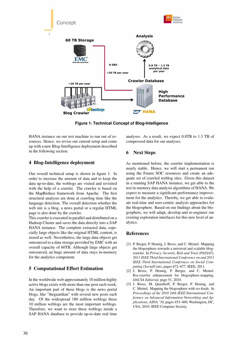
Concept

1

Blog Crawler

60 TB Storage

Crawler Database

HANA

8 GBit

Analysis

High PerformanceDatabase

0.8 TB – 1.3 TB analytical data

per year

~20 TB per year

~20 TB per year

Figure 1: Technical Concept of Blog-Intelligence

HANA instance on our test machine to run out of re-sources. Hence, we revise our current setup and comeup with a new Blog-Intelligence deployment describedin the following section.

4 Blog-Intelligence deployment

Our overall technical setup is shown in figure 1. Inorder to increase the amount of data and to keep thedata up-to-date, the weblogs are visited and revisitedwith the help of a crawler. The crawler is based onthe MapReduce framework from Apache. The firststructural analyses are done at crawling time like thelanguage detection. The overall detection whether theweb site is a blog, a news portal or a regular HTMLpage is also done by the crawler.This crawler is executed in parallel and distributed on aHadoop Cluster and saves the data directly into a SAPHANA instance. The complete extracted data, espe-cially large objects like the original HTML content, isstored as well. Nevertheless, the large data objects getoutsourced to a data storage provided by EMC with anoverall capacity of 60TB. Although large objects getoutsourced, an huge amount of data stays in-memoryfor the analytics component.

5 Computational Effort Estimation

In the worldwide web approximately 10 million highlyactive blogs exists with more than one post each week.An important part of these blogs is the news portalblogs, like ”theguardian” with several new posts eachday. Of the widespread 180 million weblogs these10 million weblogs are the most important weblogs.Therefore, we want to store these weblogs inside aSAP HANA database to provide up-to-date real time

analyses. As a result, we expect 0.8TB to 1.3 TB ofcompressed data for our analyses.

6 Next Steps

As mentioned before, the crawler implementation isnearly stable. Hence, we will start a permanent runusing the Future SOC resources and create an ade-quate set of crawled weblog sites. Given this datasetin a running SAP HANA instance, we get able to thetest in-memory data analysis algorithms of HANA. Weexpect to measure a significant performance improve-ment for the analytics. Thereby, we get able to evalu-ate real-time and user-centric analysis approaches forthe blogosphere. Based on our findings about the blo-gosphere, we will adapt, develop and re-engineer ourexisting exploration interfaces for this new level of an-alytics.

References

[1] P. Berger, P. Hennig, J. Bross, and C. Meinel. Mappingthe blogosphere–towards a universal and scalable blog-crawler. In Privacy, Security, Risk and Trust (PASSAT),2011 IEEE Third International Conference on and 2011IEEE Third International Confernece on Social Com-puting (SocialCom), pages 672–677. IEEE, 2011.

[2] J. Bross, P. Hennig, P. Berger, and C. Meinel.Rss-crawler enhancement for blogosphere-mapping.IJACSA Editorial, page 51, 2010.

[3] J. Bross, M. Quasthoff, P. Berger, P. Hennig, andC. Meinel. Mapping the blogosphere with rss-feeds. InProceedings of the 2010 24th IEEE International Con-ference on Advanced Information Networking and Ap-plications, AINA ’10, pages 453–460, Washington, DC,USA, 2010. IEEE Computer Society.

36

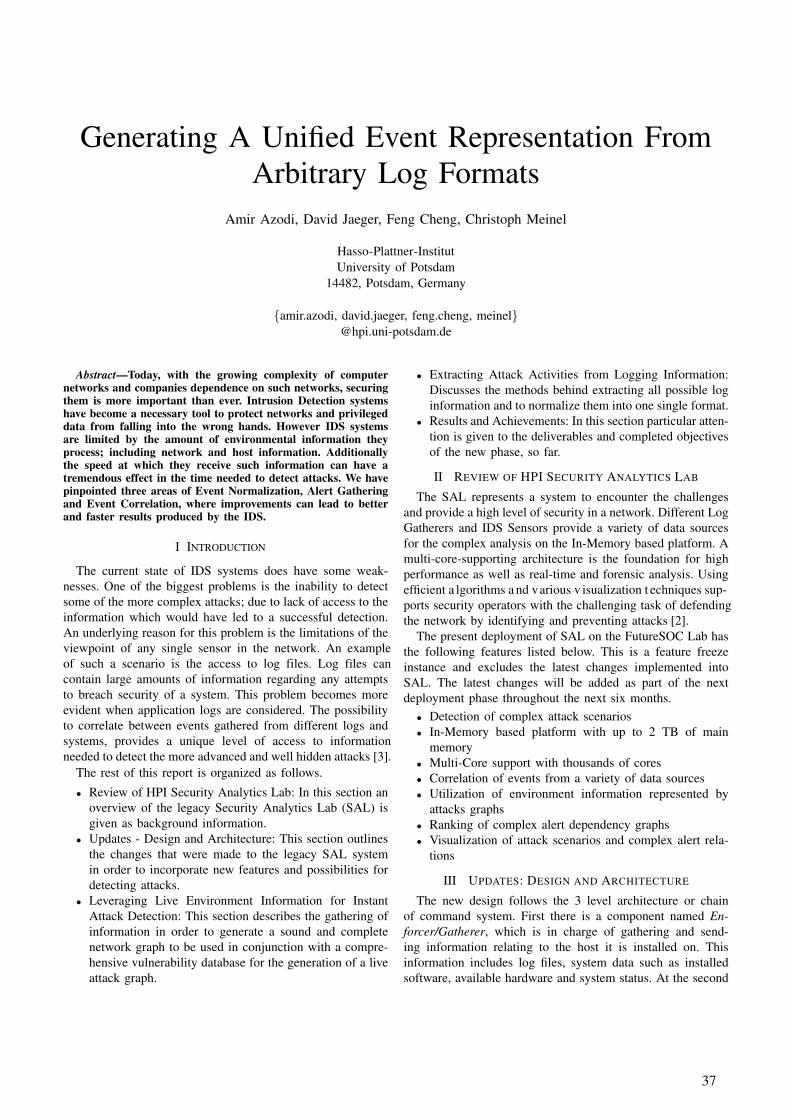
Generating A Unified Event Representation FromArbitrary Log Formats

Amir Azodi, David Jaeger, Feng Cheng, Christoph Meinel

Hasso-Plattner-Institut University of Potsdam

14482, Potsdam, Germany

{amir.azodi, david.jaeger, feng.cheng, meinel}@hpi.uni-potsdam.de

Abstract—Today, with the growing complexity of computernetworks and companies dependence on such networks, securingthem is more important than ever. Intrusion Detection systemshave become a necessary tool to protect networks and privilegeddata from falling into the wrong hands. However IDS systemsare limited by the amount of environmental information theyprocess; including network and host information. Additionallythe speed at which they receive such information can have atremendous effect in the time needed to detect attacks. We havepinpointed three areas of Event Normalization, Alert Gatheringand Event Correlation, where improvements can lead to betterand faster results produced by the IDS.

I INTRODUCTION

The current state of IDS systems does have some weak-nesses. One of the biggest problems is the inability to detect some of the more complex attacks; due to lack of access to the information which would have led to a successful detection. An underlying reason for this problem is the limitations of the viewpoint of any single sensor in the network. An example of such a scenario is the access to log files. Log files can contain large amounts of information regarding any attempts to breach security of a system. This problem becomes more evident when application logs are considered. The possibility to correlate between events gathered from different logs and systems, provides a unique level of access to information needed to detect the more advanced and well hidden attacks [3].

The rest of this report is organized as follows.

• Review of HPI Security Analytics Lab: In this section anoverview of the legacy Security Analytics Lab (SAL) isgiven as background information.

• Updates - Design and Architecture: This section outlinesthe changes that were made to the legacy SAL systemin order to incorporate new features and possibilities fordetecting attacks.

• Leveraging Live Environment Information for InstantAttack Detection: This section describes the gathering ofinformation in order to generate a sound and completenetwork graph to be used in conjunction with a compre-hensive vulnerability database for the generation of a liveattack graph.

• Extracting Attack Activities from Logging Information:Discusses the methods behind extracting all possible loginformation and to normalize them into one single format.

• Results and Achievements: In this section particular atten-tion is given to the deliverables and completed objectivesof the new phase, so far.

II REVIEW OF HPI SECURITY ANALYTICS LAB

The SAL represents a system to encounter the challenges and provide a high level of security in a network. Different Log Gatherers and IDS Sensors provide a variety of data sources for the complex analysis on the In-Memory based platform. A multi-core-supporting architecture is the foundation for high performance as well as real-time and forensic analysis. Using efficient a lgorithms a nd various v isualization t echniques sup-ports security operators with the challenging task of defending the network by identifying and preventing attacks [2].

The present deployment of SAL on the FutureSOC Lab hasthe following features listed below. This is a feature freezeinstance and excludes the latest changes implemented intoSAL. The latest changes will be added as part of the nextdeployment phase throughout the next six months.

• Detection of complex attack scenarios• In-Memory based platform with up to 2 TB of main

memory• Multi-Core support with thousands of cores• Correlation of events from a variety of data sources• Utilization of environment information represented by

attacks graphs• Ranking of complex alert dependency graphs• Visualization of attack scenarios and complex alert rela-

tions

III UPDATES: DESIGN AND ARCHITECTURE

The new design follows the 3 level architecture or chainof command system. First there is a component named En-forcer/Gatherer, which is in charge of gathering and send-ing information relating to the host it is installed on. Thisinformation includes log files, system data such as installedsoftware, available hardware and system status. At the second

37

level a component named Agent receives the information from the Enforcer and normalizes it into CEE [5] events or control messages before sending them to the Server. Finally the Server will make the information persistent and continues on to generating an attack graph and correlating events received in order to find attacks. Figure 1 illustrates this workflow.

Enforcer /Gatherer

Agent

Log Data,Installed Software,

Network Info,...

System Logs,Application Logs

Server

Network Info

System Information,Installed Software, ...

Enforced Commands

Events,Installed Software,

Network Info,...

Enforced Commands

Fig. 1: Message workflow in the SAL

IV LEVERAGING LIVE ENVIRONMENT INFORMATION FORINSTANT ATTACK DETECTION

The design proposed in this report allows for complete access to the host information of every host on which the Gatherer is deployed. This information includes, but is not limited to, log files (e.g. syslog), memory information, pro-cessor information, network information (e.g. hostname, IP addresses and MAC addresses) and application information (e.g. their CPE [6], which allows SAL to compile a list of current vulnerabilities present on any host).

Having imported all the information into SAL, a networkgraph can be created. Using a vulnerability database we canthen construct a comprehensive attack graph to be used bySAL. In order to always have the most up-to-date attackgraph, the SAL system continuously updates its underlyingdata structures, i.e. the network graph and the vulnerabilitydatabase. Therefore at any moment an up-to-date attack graphcan be compiled from the live information present in theunderlying data structures.

V SUPPORTING INTRUSION DETECTION WITH EVENT LOG INFORMATION

A common way for reporting intrusions are security alerts,which are generated by so called intrusion detection systems.Generally, these alerts are generated as a result of observedactivities in an environment that are potentially harmful.However, an alert is not a guarantee that an actual intrusionhas taken place. In addition, alerts are only limited to detectedmalicious activity, but they do not give information about theattackers activities before and after his intrusion attempt. Anapproach to solve the shortcomings of an intrusion detectionwith alerts only is the consideration of additional details aboutthe attacker activities. One type of such information are eventlogs. They are produced by applications, monitoring systems,operating systems, etc. and are give an insight into all observedevents in an environment. The next subsections show howthese event logs can be gathered from different locations in anenvironment, how they are normalized into an automaticallyprocessable format [4].

A. Information Gathering

Event logs usually originate from a multitude of sources,such as IDSs, firewalls or applications, where each sourceproduces a different log representation and output format.Examples for log representations are Syslog or the IDMEFspecification and typical output formats are binary, CSV andXML. In order to read events from the log sources, thepreviously mentioned gatherers are employed. They can beattached to the log files on their host and are able to send thefile content to their centrally connected agent.

B. Normalization

The received event logs are interpreted event by event, which makes it necessary to split the sequential event stream into single events. The SAL realizes this splitting with the help of regular expressions that are on the matching of event separators. Once the events have been extracted from the event stream, they are still in a format being specific to the generat-ing event source. Therefore, each event is further transformed into a common and easily processable representation. In the concrete SAL implementation, the Common Event Expression (CEE) [5] has been chosen as the common representation of events, to which all custom event are normalized to. The CEE makes use of event containers that contains the properties of the event as key-value-pairs.

In order to normalize events to the CEE format, informationfrom the raw events have to be extracted and put into thecorresponding fields. This extraction of event properties fromthe raw events is performed with the support of regularexpression, or more specifically with the group mechanisms inregular expressions. The idea is to first define the format of asingle raw event in the expression and then surround structuredinformation with regular expression groups, so that they canbe matched and finally used as the properties of the event.

VI RESULTS AND ACHIEVEMENTS

The mechanisms that have been described in the last twosections allow the SAL to react on live changes in the network,verify intrusions and uncover intrusions that could not bedetected with the legacy SAL. In addition, it is possible tocorrelate the discovered intrusion attempts to the nodes in anattack graph. The described changes are mainly realized byinterpreting dynamic and static environment information aswell as using event logs instead of only alert logs.

VII CONCLUSION

As we work to secure networks from ever more sophisti-cated attacks, it is clear that the industry is in need of moreintelligent protection mechanisms that actively protect ournetworks. As part of this project we aim to design intelligentsolutions that consider a wide array of information relatinga network and are therefore better able to detect intrusions.The initial results of our method show considerable promise.In the next phases of the project, we will focus finishing aPOC implementation of our design principles and functionalrequirements. We also look to publish the results of our POC

38

implementation and the effectiveness of the system as a wholein subsequent reports aimed at the Future SOC Lab.

REFERENCES

[1] Sebastian Roschke, Feng Cheng, Robert Schuppenies, and ChristophMeinel: Towards Unifying Vulnerability Information for Attack GraphConstruction , in Proceedings of 12th Information Security Conference(ISC’09), Springer LNCS, Pisa, Italy, pp. 218-233 (September 2009)

[2] Christoph Meinel, Andreas Polze, Alexander Zeier, Gerhard Oswald,Dieter Herzog, Volker Smid, Doc DErrico and Zahid Hussain (Eds.): Proceedings of the Fall 2010 Future SOC Lab Day , Technical Report of Hasso-Plattner-Institute, Heft 42 (2011)

[3] Sebastian Roschke: Towards High Quality Security Event CorrelationUsing In-Memory and Multi-Core Processing , PhD Thesis, HassoPlattner Institute at University Potsdam (May 2012)

[4] David Jaeger: Monitoring in Scenario-based Security Experiments ,Master Thesis, Hasso Plattner Institute at University Potsdam (August2012)

[5] The CEE Board: CEE Overview. Available from:http://cee.mitre.org/docs/overview.html

[6] Common Platform Enumeration:. Available from: http://cpe.mitre.org/

39

Detecting biogeographical barriers - testing and putting beta diversity on a

map

Johannes Penner

Museum für Naturkunde, Leibniz-Institute

for Evolution & Biodiversity Research,

Department of Research, Herpetology

Group

Invalidenstrasse 43

10115 Berlin, Germany

[email protected]

Moritz Augustin

Technische Universität Berlin, Department

of Software Engineering & Theoretical

Computer Science, Neural Information

Processing Group

Marchstr. 23


[email protected]

Abstract

Biogeographical regions are not only of scientific but

also of conservation importance. The most common

approach is to map species richness. However, beta

diversity (species turnover) is better suited to identify

where boundaries between regions are.

We calculated beta diversity for West African am-

phibians on a fine scale (30 arcseconds), using mov-

ing window and parallelization techniques. This

would have been impossible with standard hard- and

software. Not only was this the first time to produce

such fine scaled maps but we systematically com-

pared different indices and different moving window

sizes.

Currently our results are only preliminary, the work

plan has not been fulfilled yet and detailed analyses

are pending. Furthermore we would like to ask for an

extension of access possibilities and enhance our

study significantly by switching from binary input

data to proxies for abundance data.

1 Background

Amphibians form an integral part of biodiversity and

are one of the most threatened vertebrate groups on

the globe, with more than one third of all known

species listed as threatened on the IUCN Red List [1,

2]. Biodiversity is declining in many areas and in-

cludes amphibians. The so called amphibian decline

is a global problem and due to a number of reasons.

The main ones are habitat destruction, alteration and

fragmentation as well as pesticides, climate change,

overharvesting and emerging diseases [3]. Causes are

also often interacting. Thus, well-informed conserva-

tion decisions are needed, especially for areas which

harbor the highest diversity but are poorly studied,

i.e. the tropical regions. One base for such decisions

is the answer to where and why species occur.

In general, amphibian diversity and biodiversity are

measured on three different scales: genes, organisms

and landscapes. Organismic diversity is the most

common measure. Measured at one site it is called

alpha diversity, the comparison between two sites is

named beta diversity and gamma diversity is calcu-

lated across a landscape [4].

Besides the general interest where the highest species

diversity is found, the distribution of diversity is

important for conservation. One main aim is to set

priority areas when efforts have to be concentrated.

Another aim is to provide decision makes with the

scientific sound arguments for areas in need of pro-

tection.

In general, a trait off exists between the conservation

side which requests fine grained maps and the scien-

tific need to cover large areas. Studies fulfilling both

requirements, covering a large area with a high reso-

lution, are scarce. Our study is one of the few at-

tempts to provide both. We study West African am-

phibians, which are unique and face multiple threats;

mainly severe habitat destruction and fragmentation

(e.g. see [5]).

2 Previous work

We used Environmental Niche Modelling (ENM;

also commonly called Species Distribution Model-

ling) to derive the occurrence of West African am-

phibians on a grid of 30x30 arcseconds (≈ 1km²). So

far ENMs were constructed for 158 out of ca. 180

known species with more than 9000 occurrence rec-

ords. The ENMs used 18 environmental parameters:

ten climate (different temperature and precipitation

41

measures), five vegetation (different wavelengths

from two satellites), two altitudinal (calculated from

a digital elevation model and one “hydrology” pa-

rameters) (compare to [6]). A machine learning max-

imum entropy algorithm [7,8,9] compared environ-

mental parameters at sites of occurrences against

randomly sampled background data (see [10] for a

statistical explanation of the algorithm). This resulted

in map showing the distribution of modeled species

richness covering the whole West African region

(Penner et al. in prep.).

3 Project idea

Inspired by McKnight et al. [11] we wanted to inves-

tigate species turnover (≈ beta diversity) for the

whole region. The main aim is to identify biogeo-

graphical regions and boundaries, which are reflected

by relatively high species turnover. This is done by

comparing species occurrences between neighboring

grid cells.

To our knowledge this approach has never been tack-

led systematically, especially with real data, contrary

to simulated data. No agreement exists for example

which index should be used though some progress

has been made. Therefore we will compare different

indices and different moving window sizes.

The final programmed software will be open source

published using a public domain license. It will allow

the user to specify own indices and moving window

sizes.

4 Used Future SOC Lab resources

The large scale of our analysis does not permit the

use of available standard computer hard- and soft-

ware. Applying a moving window approach we uti-

lized the HPI Future SOC Lab Fujitsu RX600S5

machines, parallelizing data. Though it would be

interesting to test how the Hewlett Packard DL980

G7 servers would speed up calculations.

5 Findings

Currently we programmed two binary indices Jaccard

[12] and Mountford [13]. Beta diversity is calculated

as the species turn over between one grid cell and its

neighboring cells. A third index, Raup-Crick [14],

will be implemented soon. All three indices use bina-

ry occurrence data and weigh presence and absence

data differently (see [15]). Moving window sizes

varied from 3 to 93 (Mountford) and 201 (Jaccard).

Larger sizes will be explored but are very computing

intensive.

Unique areas are consistently showing up regardless

of the index and the moving window size (see poster

presented at the Future SOC Lab day, 10th

of April

2013). Preliminary analyses indicate that biogeo-

graphic barriers might correspond to major river

systems in the region. However, at the current, stage

proper conclusions are premature.

42

Figure 1 (from previous page): Example of

frequency histograms of two different beta

diversity indices with two different moving

window sizes. From top to bottom (index

name & moving window size): Jaccard 3x3,

Jaccard 93x93, Mountford 3x3, Mountford

93x93.

Figure 1 shows four examples of frequency histo-

grams for two indices (Jaccard & Mountford) and

two different moving window sizes (3x3 & 93x93). It

The non-metric properties of the Mountford index are

clearly visible. It is obvious that both factors are

important. More thorough analyses will be prepared.

6 Next steps

Our first runs were successful. Due to delays in the

start of the project, analyses have not been completed

yet and time and logistical constraints did not allow

us to finish all intended runs. As mentioned above the

third index awaits implementation.

In addition, we have discovered a solution to move

the analyses even one large step further. So far we

used binary data, resulting in relatively simple spe-

cies richness maps. This was a result of the current

work flow but has many theoretical disadvantages.

Therefore, we would like to use proxies for abun-

dance. This would open a completely new window,

incorporating such measures as heterogeneity and

evenness in our analyses and potentially a much

higher precision. Using “abundance” data, different

indices are needed. Five potential candidates are:

Shannon, Whittaker, Wilson & Shmida, NESS and

CqN which weigh evenness differently (e.g. see [16]).

Furthermore, using the likelihoods gained from the

ENMs will enable us to calculate alpha diversity

anew, also incorporating heterogeneity and evenness.

7 Extension request

So far the possibilities of the HPI Future SOC Lab

not only enabled our work but also took it a huge step

forward. As mentioned above not all analyses were

finalized yet and they should be further improved. A

further use of the HPI Future SOC Lab facilities

would help us tremendously. Therefore we would be

very grateful if an extension of our access to the HPI

Future SOC Lab resources is granted. A follow-up

proposal has been submitted.

8 Acknowledgements

We thank the innumerous colleagues who shared

their data. We are also indebted to a number of peo-

ple who assisted in the field, in the laboratory and in

various other ways, the most important ones are:

Mark-Oliver Rödel, Jakob Fahr, Matthias Herkt,

Günther Barnikel, Mirjana Bevanda, Mareike Hirsch-

feld, Jenja Kronenbitter, Anja Pfahler, Meike

Mohneke & K. Eduard Linsenmair. Various funding

agencies enabled the work. The main part of it was

initially funded by the German Ministry for Educa-

tion and Research (BMBF): BIOTA West Africa, 01

LC 0617J.

We are very grateful to the HPI Future SOC Lab for

granting us access to their computing capacities!

References

[1] S.N. Stuart, J.S. Chanson, N.A. Cox, B.E. Young,

A.S.L. Rodrigues, D.L. Fischman, & R.W. Waller:

Status and trends of amphibian declines and extinc-

tions worldwide. Science, 306: 1783-1786, 2004.

[2] IUCN: The IUCN Red List of threatened species.

Version 2012.2. http://www.iucnredlist.org. Last ac-

cessed 17th October 2012.

[3] S.N. Stuart, M. Hoffmann, J.S. Chanson, N.A. Cox,

R.J. Berridge, P. Ramani & B.E. Young: Threatened

amphibians of the world. Lynx Edicions, Barcelona,

IUCN, Gland, Switzerland; and Conservation Interna-

tional, Arlington, TX, 2008.

[4] A.E. Magurran: Measuring biological diversity.

Blackwell Publishers, Oxford, 2003.

[5] J. Penner, M. Wegmann, A. Hillers, M. Schmidt &

M.-O. Rödel: A hotspot revisited – a biogeographical

analysis of West African amphibians. Diversity and

Distributions, 17: 1077-1088, 2011.

[6] S.J. Phillips, M. Dudík & R.E. Schapire: A maximum

entropy approach to species distribution modeling. In:

C. Brodley, Editor. Proceedings of the Twenty-First

International Conference on Machine Learning. New

York, ACM Press: 655-662, 2004.

[7] S.J. Phillips, R.P. Anderson & R.E. Schapire: Maxi-

mum entropy modeling of species geographic distribu-

tions. Ecological Modelling, 190: 231-259, 2006.

[8] S.J. Phillips & M. Dudík: Modeling of species distri-

butions with Maxent: new extensions and a compre-

hensive evaluation. Ecography, 31: 161-175, 2008.

[9] J. Penner, G.B. Adum, M.T. McElroy, T. Doherty-

Bone, M. Hirschfeld, L. Sandberger, C. Weldon, A.A.

Cunningham, T. Ohst, E. Wombwell, D.M. Portik, D.

Reid, A. Hillers, C. Ofori-Boateng, W. Oduro, J. Plöt-

ner, A. Ohler, A.D. Leaché & M.-O. Rödel: West Af-

rica - A safe haven for frogs? A sub-continental as-

sessment of the Chytrid fungus (Batrachochytrium

dendrobatidis). PLoS ONE, 8: e56236, 2013.

[10] J. Elith, S.J. Phillips, T. Hastie, M. Dudík, Y.E. Chee

& C.J. Yates: A statistical explanation of MaxEnt for

ecologists. Diversity and Distributions, 17: 43-57,

2011.

[11] M.W. McKnight, P.S. White, R.I. McDonald, J.F.

Lamoreux, W. Sechrest, R.S. Ridgley & S.N. Stuart:

Putting beta-diversity on the map: broad scale congru-

ence and coincidence in the extremes. PLoS Biology,

5: e272, 2007.

[12] P. Jaccard: Nouvelles recherches sur la distributionflo-

rale. Bulletin de la Societe Vaudoise Sciénces Natu-

relles, 44: 223-270.

43

[13] M.D. Mountford: An index of similarity and its appli-

cation to classification problems. In: P.W. Murphy,

editor. Progress in soil zoology. Butterworth, London:

43-50, 1962.

[14] D. Raup, & R.E. Crick: Measurement of faunal simi-

larity in paleontology. Journal of Paleontology, 53:

1213-1227, 1979

[15] P. Legendre & L. Legendre: Numerical Ecology, 2nd

Edition. Elsevier Science B.V., Amsterdam, 1998

[16] A.E. Magurran & B.J. McGill: Biological Diversity –

frontiers in measurement and assessment. University

Press, Oxford, 2011.

44

Heterogeneous Software Pipelining for Memory-bound Kernels

Fahad Khalid

Hasso-Plattner-Institut

University of Potsdam


[email protected]

Andreas Polze




[email protected]

Abstract

The use of accelerator architectures such as GPUs is

now ubiquitous in high performance computing

(HPC). For certain combinatorial algorithms, the

size of output generated can be much larger than the

size of the input dataset. This is especially true when

combinatorial operations are performed element-

wise. The massive increase in output size requires

frequent transfer of result data from the GPU

memory to the CPU memory. Since this transfer op-

eration is much slower as compared to the speed of

computing on the GPU, it becomes a performance

bottleneck.

The heterogeneous software pipelining approach has

been developed to deal with the above mentioned

problem. In this approach, we execute the kernel in

two parts, spanned over both the GPU and the CPU.

The computation is performed in a pipelined fashion.

In this report, we consider a highly memory-bound

combinatorial kernel from the domain of Computa-

tional Biology, and improve its performance on a

heterogeneous platform using the heterogeneous

software pipelining approach. The results show that

our approach not only makes it possible to gain

speedup over a serial implementation; it performs

even better than a multi-threaded CPU-only SMP

version.

1 Motivation

In recent years, research community in the High Per-

formance Computing (HPC) and Scientific Compu-

ting sectors has witnessed an increasing application

of Heterogeneous Computing [1] (where Heteroge-

neous Computing refers to the design of applications

that can harness the power of both the CPUs and ac-

celerators such as GPUs).

Many scientific applications comprise of computa-

tional kernels that benefit significantly from a pro-

cessor’s capability to perform a large number of

arithmetic operations at high speeds. Such kernels are

typically compute-bound i.e. the performance bottle-

neck lies in the complexity of arithmetic operations

(e.g. dense matrix-matrix multiplication [3]). Accel-

erator architectures such as GPUs dedicate most of

the chip area to arithmetic processing units. This

makes it possible for properly tuned compute-bound

kernels to perform at levels close to the peak perfor-

mance offered by the underlying architecture. A sig-

nificant number of algorithms have been successfully

ported to GPUs, attaining up to 100x speedup over

serial execution on a CPU [2]. Such speedup is lim-

ited to compute-bound kernels.

There is however another set of kernels, where the

performance bottleneck is dictated by the frequency

of memory access operations. Such kernels are

termed memory-bound. These kernels typically have

a low arithmetic intensity (i.e. a low compute to

main-memory access ratio). A common example for

such a kernel is Sparse Matrix-Vector Multiplication

(SpMV) [4], which is the foundation for linear solv-

ers. In addition, certain combinatorial algorithms are

memory bound as well. As stated earlier, accelerator

architectures favor compute-bound kernels. This rais-

es the following questions:

Is it possible to effectively utilize Heterogeneous

Computing for algorithms with low arithmetic inten-

sity? Or must such algorithms be executed on CPU-

only systems?

2 Heterogeneous Software Pipelining

2.1 Concept

The approach proposed in this section is applicable to

memory-bound algorithms that can be split into two

parts:

1. A part with high arithmetic intensity

2. A part with very low arithmetic intensity

For a given such algorithm, the part with high arith-

metic intensity is implemented as a GPU kernel. The

other part is implemented as a CPU kernel. This par-

ticular distribution of the kernels amongst the two

types of processors is based on the processors’ capa-

bilities to process such kernels. GPUs can effectively

utilize their massively parallel architecture to process

kernels with high arithmetic intensity, while CPUs

outperform GPUs on kernels with very low arithme-

45

tic intensity. By splitting the algorithm into two ker-

nels and executing these on the most suitable proces-

sor architectures respectively, a significant gain in

performance is expected over a homogeneous parallel

implementation.

Once the kernels have been implemented, these are

executed in the following steps:

1. The GPU kernel is executed, which com-

putes some intermediate results.

2. As soon as the intermediate results are gen-

erated, two things happen concurrently. The

results are transferred from the GPU

memory to the CPU memory, and the GPU

starts processing the next batch of input da-

ta.

3. After the transfer of the first batch of inter-

mediate results from GPU memory to CPU

memory is complete, the CPU kernel is exe-

cuted, which processes these intermediate

results.

Figure 1: A 3-stage heterogeneous software

pipeline.

The process is illustrated in Figure 1. The data pro-

cessing loop is executed in a pipeline with 3-stages.

All three stages are executed asynchronously, and

therefore the waiting time between the different stag-

es is minimized.

2.2 Results

The heterogeneous software pipelining approach was

applied to a kernel from the domain of Computation-

al Biology. This kernel is termed as Combinatorial

Candidate Generation. The algorithm has already

been successfully parallelized on both shared-

memory [5] and distributed-memory [6] CPU based

architectures. Here, a heterogeneous architecture

based parallelization is presented. Three instances of

the kernel were implemented: Serial, CPU-only par-

allel and heterogeneous software pipeline. Table 1

presents the execution times of the three different

implementations, against four different datasets. The

datasets represent real metabolic networks from the

bacterium E.Coli.

As can be seen in the table, the CPU-only implemen-

tation outperforms the pipelined implementation on

the first dataset, and the two implementations yield

identical performance on the second dataset. This is

due the fact that these datasets are very small, and the

overhead incurred in pipelining over-shadows much

of the performance gain. For larger datasets however,

the heterogeneous pipelining approach yields a sig-

nificant performance gain, resulting in a 6-fold

speedup over the serial implementation, and 1.8-fold

speedup over the CPU-only parallel implementation.

Table 1: Comparative results of three different

implementations against four networks. Execution

times (in seconds) are presented against each im-

plementation and network; m is the number of

metabolites, r is the number of reactions.

Network

Size

#candidates Time (s)

Serial CPU-only

Pipelined

26m×38r 219743731 1.2 0.38 0.39

26m×40r 130992739 0.77 0.35 0.35

26m×31r 752482917 4.1 1.6 1.0

26m×43r 2616975505 14 5.5 2.5

3 Future Work

Following are some plausible directions for future

work:

In-depth analysis of the heterogeneous soft-

ware pipelining approach to investigate ap-

plicability to other kernels: This will involve

an empirical evaluation of the performance

of different stages, finding the optimal pa-

rameter configuration to get the best possi-

ble performance, as well as finding the full

set of limitations that may lead to improved

solutions.

Investigation of arithmetic intensity as a

useful metric to determine the most suitable

processor architecture for a specific paral-

lel kernel: The objective here is to develop a

quantitative model that given the arithmetic

intensity of a kernel, provides a good esti-

mate of performance expected on a given

architecture. As per the current state-of-the-

art, the decision of which architecture to

choose is more a matter of expert opinion

and empirical evaluation, than model based

prediction. Once a suitable model is availa-

ble, not only will it serve as a decision sup-

port tool, it might also provide further in-

sight into the relative impact of certain ar-

chitectural characteristics on the perfor-

mance of memory-bound algorithms.

4 Publication

Based on the research described above, the following

paper has been submitted for review:

46

Fahad Khalid, Zoran Nikoloski, Peter Trö-

ger, Andreas Polze. Heterogeneous Combi-

natorial Candidate Generation.

5 Conclusions

We have introduced a novel approach for managing

arithmetic intensity of memory-bound combinatorial

algorithms on heterogeneous architectures; especially

for cases where transfer of data from the GPU

memory to CPU memory forms the performance bot-

tleneck. Our approach termed heterogeneous soft-

ware pipelining has been successfully implemented

for an application from the domain of Computational

Biology. The results show a significant increase in

performance as compared to serial and CPU-only

parallel implementations.

In our collective work up till now, we have focused

on improving the performance of the elementary

mode enumeration problem from computational biol-

ogy. To this end, we have made the following contri-

butions:

Improved the memory consumption behav-

ior of the application on shared-memory

SMP architectures.

Developed the first ever heterogeneous im-

plementation of the combinatorial candidate

generation algorithm.

In addition, we have generalized our results to

memory-bound combinatorial algorithms, for which

the following novel method has been developed:

Heterogeneous Software Pipelining

Based on our research and the above mentioned con-

tributions, it can be seen that novel methods are

needed for the effective utilization of heterogeneous

resources when used for memory-bound algorithms.

References

[1] J. D. Owens, D. Luebke, N. Govindaraju,

M. Harris, J. Krüger, A. E. Lefohn, and T. J. Purcell,

"A Survey of General-Purpose Computation on

Graphics Hardware," Computer Graphics Forum, vol.

26, pp. 80-113, 2007.

[2] V. W. Lee, C. Kim, J. Chhugani, M. Deish-

er, D. Kim, A. D. Nguyen, N. Satish, M. Smelyan-

skiy, S. Chennupaty, P. Hammarlund, R. Singhal, and

P. Dubey, "Debunking the 100X GPU vs. CPU myth:

an evaluation of throughput computing on CPU and

GPU," presented at the Proceedings of the 37th annu-

al international symposium on Computer architec-

ture, Saint-Malo, France, 2010.

[3] A. Buluç, J. R. Gilbert, and C. Budak,

"Solving path problems on the GPU," Parallel Com-

puting, vol. 36, pp. 241-253, 2010.

[4] J. D. Davis and E. S. Chung, "SpMV: A

Memory-Bound Application on the GPU Stuck Be-

tween a Rock and a Hard Place," Microsoft Research

Silicon Valley, Technical Report14 September 2012

2012.

[5] M. Terzer and J. Stelling, "Accelerating the

Computation of Elementary Modes Using Pattern

Trees," in Algorithms in Bioinformatics. vol. 4175,

P. Bücher and B. Moret, Eds., ed: Springer Berlin /

Heidelberg, 2006, pp. 333-343.

[6] D. Jevremović, C. T. Trinh, F. Srienc, C. P.

Sosa, and D. Boley, "Parallelization of Nullspace

Algorithm for the computation of metabolic path-

ways," Parallel Computing, vol. 37, pp. 261-278,

2011.

47

Using In-Memory Computing for Proactive Cloud OperationsFuture SOC Lab Report April 2013

Eyk Kny, Felix Salfner, Marcus KrugSAP Innovation Center, Potsdam

Norman Höfler, Peter Tröger Hasso-Plattner-Institut, Potsdam

Abstract

The operation of a complex IT landscape, such as acloud computing data center, is a true operator chal-lenge. An ever-growing number of servers, the het-erogeneity of software, the necessary elastic load han-dling, energy consumption and other non-functionalaspects have to be taken into account – continuouslyand in an adaptive fashion.We introduce the concept of proactive cloud oper-ations, were preventive maintenance activities (suchas load migration) are automatically triggered whensome part of the system is about to enter an erroneousstate. The trigger is generated from a automated rootcause analysis that relies on the in-memory computingof anomaly signals and structure-of-influence graphsfor the different entities in the monitored IT landscape.We have implemented a prototype of proactive cloudoperation with HANA technology in the FutureSOClab. Our experiments show that an anomaly signal ap-proach for proactive monitoring can achieve the nec-essary level of accuracy with real-world data.

1 Introduction

Cloud computing is currently one of the predominanttrends in IT industry and research. The new paradigmchanges the way how IT companies operate businessesas well as how end-users (private and corporate) per-ceive software and IT. Cloud computing moves theburden of IT infrastructure management and operationaway from users to specialized providers that can guar-antee fast, reliable, and secure operation of the pro-vided service.User expectations and scalability aspects turn the man-agement of cloud computing infrastructures into atrue challenge. An ever-growing number of servers,the heterogeneity of software, multiple interactingmechanisms to elastically react on changing load, theconsideration of energy consumption and other non-functional aspects have to be taken into account. Thisrequires intelligent management tools with a high levelof automation, in order to deliver the guaranteed ser-vice level to the user while still making money.

Typical management tools rely on the availability ofa continuous stream of monitoring data from the ITlandscape. One of the key features in such monitor-ing is to aggregate low-level monitoring data to crit-ical events being presented to the operation person-nel. To achieve this goal, current monitoring systemsrely on temporal correlation, spatial correlation, andinfrastructure-centric rule-based analysis of the low-level data. These techniques usually have a snapshot-alike view on the system and therefore cannot detectproblems that evolve in the system over a longer pe-riod of time.In our project, we explore new approaches for comput-ing correlations between monitoring signals, in orderto identify the spreading of problems within a system.This report summarizes the second project phase anddocuments our results so far. In summary we have ...

• ... optimized the monitoring and computation in-frastructure for anomaly detection, which was de-veloped in the first phase.

• ... optimized the computation of signal correla-tion using SAP’s in-memory database HANA.

• ... built a web-based front-end for interac-tion with structure-of-influence graphs stored inHANA.

• ... developed a new graphical representation forthe correlation of hierarchical monitoring signals.

• ... investigated ways how to use structure-of-influence graphs for the prediction of upcomingfailures.

• ... developed a mock version of the HANA-basedsoftware for quick algorithm comparison and sig-nal generation testing.

2 Approach

The basic approach being applied since the first projectphase is the algorithm by Oliner et al. [13]. It is basedon the notion of anomaly signals, which are real val-ues between zero and one that indicate how much ameasurement signal deviates from ”normal behavior”.

49

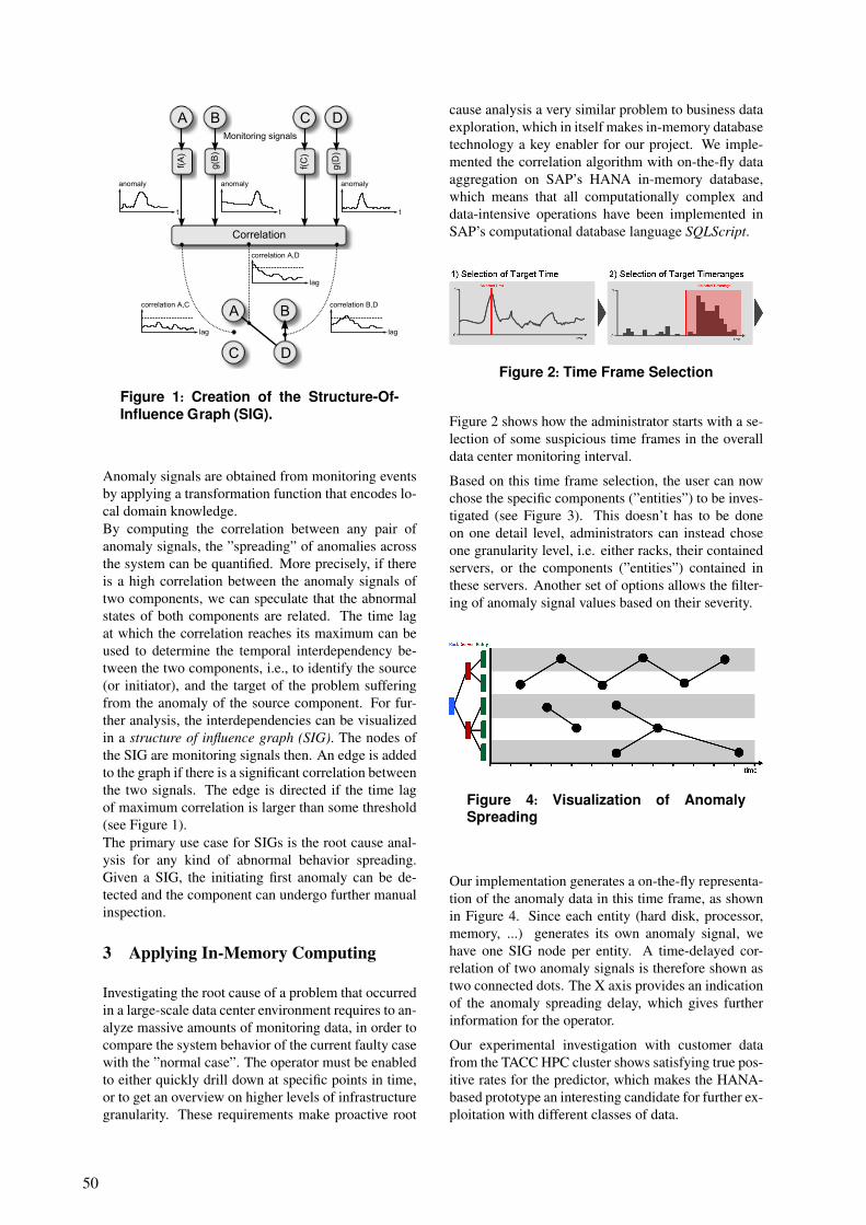
A B C D

Correlation

A B

C D

Monitoring signals

f(A

)

g(B

)

f(C

)

g(D

)

tt

anomaly

t

lag

correlation B,D

lag

correlation A,C

lag

correlation A,D

anomaly anomaly

Figure 1: Creation of the Structure-Of-Influence Graph (SIG).

Anomaly signals are obtained from monitoring eventsby applying a transformation function that encodes lo-cal domain knowledge.By computing the correlation between any pair ofanomaly signals, the ”spreading” of anomalies acrossthe system can be quantified. More precisely, if thereis a high correlation between the anomaly signals oftwo components, we can speculate that the abnormalstates of both components are related. The time lagat which the correlation reaches its maximum can beused to determine the temporal interdependency be-tween the two components, i.e., to identify the source(or initiator), and the target of the problem sufferingfrom the anomaly of the source component. For fur-ther analysis, the interdependencies can be visualizedin a structure of influence graph (SIG). The nodes ofthe SIG are monitoring signals then. An edge is addedto the graph if there is a significant correlation betweenthe two signals. The edge is directed if the time lagof maximum correlation is larger than some threshold(see Figure 1).The primary use case for SIGs is the root cause anal-ysis for any kind of abnormal behavior spreading.Given a SIG, the initiating first anomaly can be de-tected and the component can undergo further manualinspection.

3 Applying In-Memory Computing

Investigating the root cause of a problem that occurredin a large-scale data center environment requires to an-alyze massive amounts of monitoring data, in order tocompare the system behavior of the current faulty casewith the ”normal case”. The operator must be enabledto either quickly drill down at specific points in time,or to get an overview on higher levels of infrastructuregranularity. These requirements make proactive root

cause analysis a very similar problem to business dataexploration, which in itself makes in-memory databasetechnology a key enabler for our project. We imple-mented the correlation algorithm with on-the-fly dataaggregation on SAP’s HANA in-memory database,which means that all computationally complex anddata-intensive operations have been implemented inSAP’s computational database language SQLScript.

Figure 2: Time Frame Selection

Figure 2 shows how the administrator starts with a se-lection of some suspicious time frames in the overalldata center monitoring interval.

Based on this time frame selection, the user can nowchose the specific components (”entities”) to be inves-tigated (see Figure 3). This doesn’t has to be doneon one detail level, administrators can instead choseone granularity level, i.e. either racks, their containedservers, or the components (”entities”) contained inthese servers. Another set of options allows the filter-ing of anomaly signal values based on their severity.

Figure 4: Visualization of Anomaly Spreading

Our implementation generates a on-the-fly representa-tion of the anomaly data in this time frame, as shownin Figure 4. Since each entity (hard disk, processor,memory, ...) generates its own anomaly signal, wehave one SIG node per entity. A time-delayed cor-relation of two anomaly signals is therefore shown astwo connected dots. The X axis provides an indicationof the anomaly spreading delay, which gives furtherinformation for the operator.

Our experimental investigation with customer datafrom the TACC HPC cluster shows satisfying true pos-itive rates for the predictor, which makes the HANA-based prototype an interesting candidate for further ex-ploitation with different classes of data.

50

Figure 3: Anomaly Data Filtering

4 Mock Analysis Engine

In order to simplify the research on anomaly signalalgorithms, we developed a new framework that allowsthe flexible testing of different analysis methods basedon log file event traces.

The framework realizes the different steps as set ofscalable, easy to modify Python mapping scripts. Thegoal here is to make it as fast and easy as possi-ble to test new and improved future methods. Toachieve this, the framework is built upon a plugin con-cept, which makes it very easy to integrate new logfiles, anomaly generation and analysis method scripts(see Figure 5). All test runs of this framework wereperformed with real-world data from the ComputerFailure Data Repository (CFDR) on the FutureSOCRX600 resources.

The first step is a preprocessing step, in which a givenset of log files is parsed. During this process, the mon-itoring entries are translated into a unified event dataschema. Log parsing and analysis is parallelized un-der consideration of I/O issues. The user only has tospecify the map function that converts a log line intothe framework data model. The framework takes careof reading the log files in parallel, and writing the re-sults to a local database.

The next step is the anomaly signal generation pro-cess, based on the extracted events. This step requiresthe implementation of the anomaly signal generator(s)by the researcher. Our framework allows running mul-tiple signal generators at the same time, each genera-tor can also run with several different configurations.The framework takes care of all the necessary routinework, such as reading the database with the prepro-cessed log entries into shared memory.

The last step is to analyze the generated anomaly sig-nals and to generate the SIG. Again, the researcherhas only to provide a mapping function here, while theframework is managing the data-parallel execution ofthe necessary computations.

Once the generation is finished, the result is analyzedand visualized so that the user can evaluate the qual-ity of the anomaly signal generator, get new insightsand improve it. The generation and analyzing steps arepart of an iterative process and can therefore repeatedseveral times.

5 Conclusions and Next Steps

Our project brings a new correlation-based monitor-ing data analysis method to in-memory database tech-nology. Our proven prototype running on HANA inthe FutureSOC lab shows first solid results and can beused by administration people through novel data rep-resentation approaches.As part of the future work, we investigate how to fusemultiple, independent anomaly signals into one meta-signal. This allows for combining the advantages ofdifferent anomaly signal generation approaches intoone data set.A second major focus of the future work is the reduc-tion of computational complexity using advanced pre-processing techniques in a new custom tool chain. Weintend to make structure-of-influence graphs easier toconsume by exploring new graphical representationsin the near future. Furthermore, future work will fo-cus on the exploration of simplification techniques aswell as the application in new domains such as busi-ness data.

References

[1] M. Andrecut. Parallel GPU Implementation ofIterative PCA Algorithms. Journal of Computa-tional Biology, 16:1593–1599, November 2009.

[2] Joshua Bowden. Application of the OpenCLAPI for Implementation of the NIPALS Algo-rithm for Principal Component Analysis of LargeData Sets. In 2010 Sixth IEEE International Con-ference on e-Science Workshops, pages 25–30,Washington, DC, USA, 2010. IEEE ComputerSociety.

[3] Eric Brewer. Lessons from giant-scale services.Internet Computing, 5:46–55, July 2001.

[4] Chun-An Chen and Sun-Yuan Hsieh. (t,k)-Diagnosis for Component-Composition Graphsunder the MM* Model. IEEE Transactions onComputers, 60:1704–1717, December 2011.

[5] Haifeng Chen, Guofei Jiang, Cristian Ungure-anu, and Kenji Yoshihira. Failure detection andlocalization in component based systems by on-line tracking. In eleventh ACM SIGKDD in-ternational conference on Knowledge discovery

51

in data mining, pages 750–755, New York, NY,USA, 2005. ACM.

[6] Matthias Dehmer, Frank Emmert-Streib, andJurgen Kilian. A similarity measure for graphswith low computational complexity. AppliedMathematics and Computation, 182:447–459,November 2006.

[7] Danny Holten. Hierarchical Edge Bundles: Visu-alization of Adjacency Relations in HierarchicalData. Transactions on Visualization and Com-puter Graphics, 12:741–748, 2006.

[8] Jon Maeng and Miroslaw Malek. A Compari-son Method for Self-Diagnosis of MultiprocessorSystems. Technical report, 1981.

[9] M. Malek and J. Maeng. Partitioning of LargeMulticomputer Systems for Efficient Fault Di-agnosis. In Digest of Papers of the 12th Fault-Tolerant Computing Symposium, pages 341–348,New York, 1982. IEEE.

[10] Adam Oliner. Using Influence to UnderstandComplex Systems. PhD thesis, Stanford Univer-sity, September 2011.

[11] Adam Oliner and Alex Aiken. A query languagefor understanding component interactions in pro-duction systems. In 24th ACM InternationalConference on Supercomputing, pages 201–210.ACM, 2010.

[12] Adam Oliner and Alex Aiken. Online Detectionof Multi-Component Interactions in ProductionSystems. In Dependable Systems and Networks,pages 49–60. IEEE, 2011.

[13] Adam J. Oliner, Ashutosh V. Kulkarni, and AlexAiken. Using Correlated Surprise to Infer SharedInfluence. In Dependable Systems and Networks,pages 191–200. IEEE Computer Society, 2010.

[14] Panagiotis Papadimitriou, Ali Dasdan, and Hec-tor Garcia-Molina. Web Graph Similarity forAnomaly Detection. Technical Report 2008-1,January 2008.

[15] Spiros Papadimitriou, Jimeng Sun, and ChristosFaloutsos. Streaming pattern discovery in multi-ple time-series. In 31st international conferenceon Very large data bases, pages 697–708. VLDBEndowment, 2005.

[16] Yasushi Sakurai, Christos Faloutsos, and SpirosPapadimitriou. Fast Discovery of Group LagCorrelations in Streams. ACM Trans. Knowl.Discov. Data, 5, December 2010.

[17] Yasushi Sakurai, Spiros Papadimitriou, andChristos Faloutsos. BRAID: stream miningthrough group lag correlations. In 2005 ACM

SIGMOD international conference on Manage-ment of data, pages 599–610, New York, NY,USA, 2005. ACM.

[18] Lindsay Smith. A tutorial on Principal Compo-nents Analysis. 2002.

52

worker

Log

log entries

anomaly signal generator

log entries in shared memory

fusion

analyser anomaly signals

analyser results

anomaly signal in shared memory

worker worker



analyser analyser

analyser results

analyser results

preprocessing

Anomaly signal generation

analyzing

Figure 5. Architecture of the Mock Analysis Engine

53

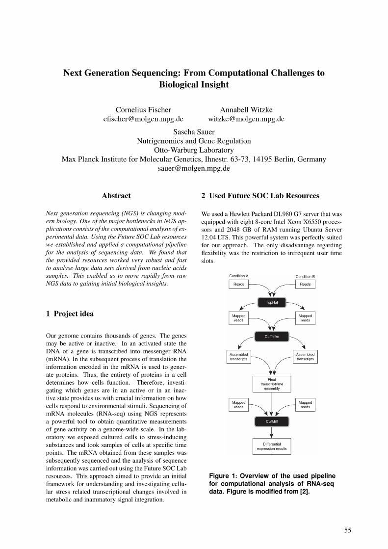
Next Generation Sequencing: From Computational Challenges toBiological Insight

Cornelius [email protected]

Annabell [email protected]

Sascha SauerNutrigenomics and Gene Regulation

Otto-Warburg LaboratoryMax Planck Institute for Molecular Genetics, Ihnestr. 63-73, 14195 Berlin, Germany

[email protected]

Abstract

Next generation sequencing (NGS) is changing mod-ern biology. One of the major bottlenecks in NGS ap-plications consists of the computational analysis of ex-perimental data. Using the Future SOC Lab resourceswe established and applied a computational pipelinefor the analysis of sequencing data. We found thatthe provided resources worked very robust and fastto analyse large data sets derived from nucleic acidssamples. This enabled us to move rapidly from rawNGS data to gaining initial biological insights.

1 Project idea

Our genome contains thousands of genes. The genesmay be active or inactive. In an activated state theDNA of a gene is transcribed into messenger RNA(mRNA). In the subsequent process of translation theinformation encoded in the mRNA is used to gener-ate proteins. Thus, the entirety of proteins in a celldetermines how cells function. Therefore, investi-gating which genes are in an active or in an inac-tive state provides us with crucial information on howcells respond to environmental stimuli. Sequencing ofmRNA molecules (RNA-seq) using NGS representsa powerful tool to obtain quantitative measurementsof gene activity on a genome-wide scale. In the lab-oratory we exposed cultured cells to stress-inducingsubstances and took samples of cells at specific timepoints. The mRNA obtained from these samples wassubsequently sequenced and the analysis of sequenceinformation was carried out using the Future SOC Labresources. This approach aimed to provide an initialframework for understanding and investigating cellu-lar stress related transcriptional changes involved inmetabolic and inammatory signal integration.

2 Used Future SOC Lab Resources

We used a Hewlett Packard DL980 G7 server that wasequipped with eight 8-core Intel Xeon X6550 proces-sors and 2048 GB of RAM running Ubuntu Server12.04 LTS. This powerful system was perfectly suitedfor our approach. The only disadvantage regardingflexibility was the restriction to infrequent user timeslots.

Figure 1: Overview of the used pipeline for computational analysis of RNA-seq data. Figure is modified from [2].

55

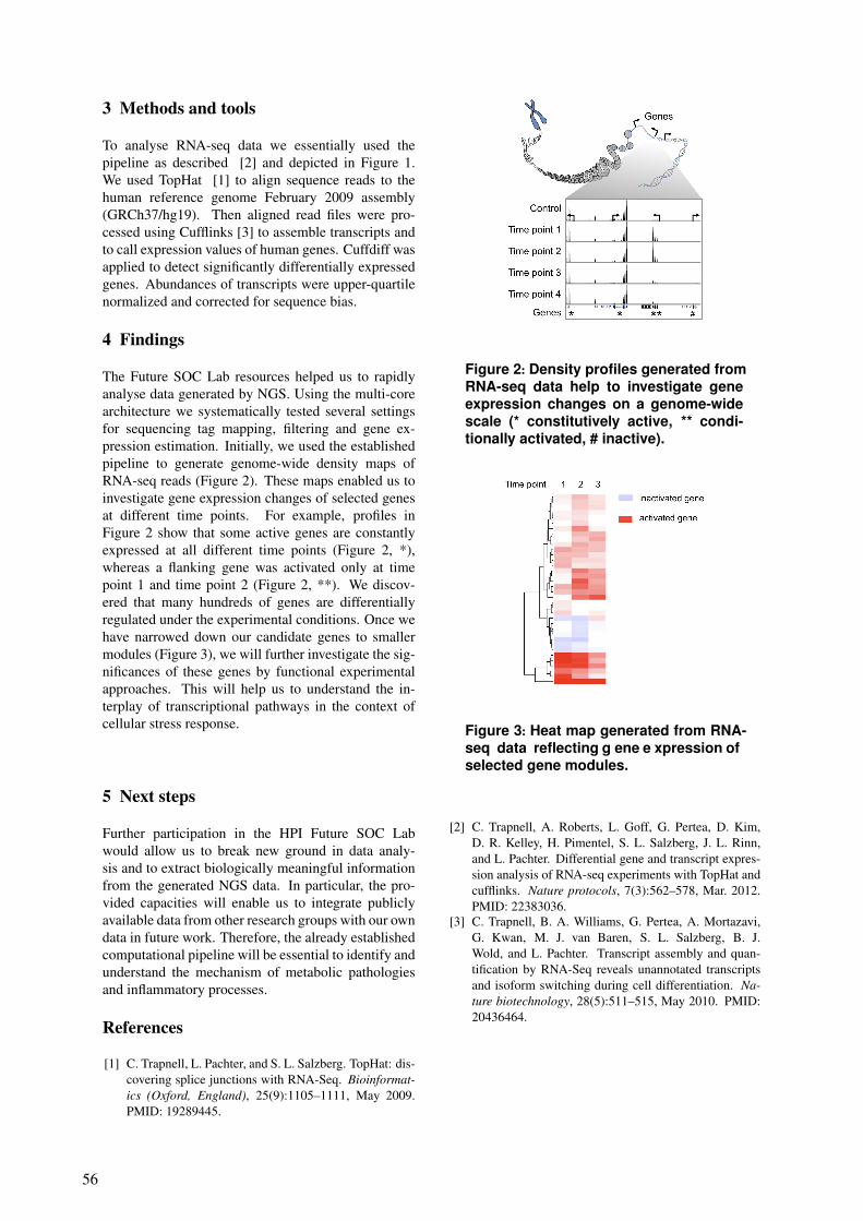
3 Methods and tools

To analyse RNA-seq data we essentially used thepipeline as described [2] and depicted in Figure 1.We used TopHat [1] to align sequence reads to thehuman reference genome February 2009 assembly(GRCh37/hg19). Then aligned read files were pro-cessed using Cufflinks [3] to assemble transcripts andto call expression values of human genes. Cuffdiff wasapplied to detect significantly differentially expressedgenes. Abundances of transcripts were upper-quartilenormalized and corrected for sequence bias.

4 Findings

The Future SOC Lab resources helped us to rapidlyanalyse data generated by NGS. Using the multi-corearchitecture we systematically tested several settingsfor sequencing tag mapping, filtering and gene ex-pression estimation. Initially, we used the establishedpipeline to generate genome-wide density maps ofRNA-seq reads (Figure 2). These maps enabled us toinvestigate gene expression changes of selected genesat different time points. For example, profiles inFigure 2 show that some active genes are constantlyexpressed at all different time points (Figure 2, *),whereas a flanking gene was activated only at timepoint 1 and time point 2 (Figure 2, **). We discov-ered that many hundreds of genes are differentiallyregulated under the experimental conditions. Once wehave narrowed down our candidate genes to smallermodules (Figure 3), we will further investigate the sig-nificances of these genes by functional experimentalapproaches. This will help us to understand the in-terplay of transcriptional pathways in the context ofcellular stress response.

5 Next steps

Further participation in the HPI Future SOC Labwould allow us to break new ground in data analy-sis and to extract biologically meaningful informationfrom the generated NGS data. In particular, the pro-vided capacities will enable us to integrate publiclyavailable data from other research groups with our owndata in future work. Therefore, the already establishedcomputational pipeline will be essential to identify andunderstand the mechanism of metabolic pathologiesand inflammatory processes.

References

[1] C. Trapnell, L. Pachter, and S. L. Salzberg. TopHat: dis-covering splice junctions with RNA-Seq. Bioinformat-ics (Oxford, England), 25(9):1105–1111, May 2009.PMID: 19289445.

Figure 2: Density profiles generated from RNA-seq data help to investigate gene expression changes on a genome-wide scale (* constitutively active, ** condi-tionally activated, # inactive).

Figure 3: Heat map generated from RNA-seq data reflecting g ene e xpression of selected gene modules.

[2] C. Trapnell, A. Roberts, L. Goff, G. Pertea, D. Kim,D. R. Kelley, H. Pimentel, S. L. Salzberg, J. L. Rinn,and L. Pachter. Differential gene and transcript expres-sion analysis of RNA-seq experiments with TopHat andcufflinks. Nature protocols, 7(3):562–578, Mar. 2012.PMID: 22383036.

[3] C. Trapnell, B. A. Williams, G. Pertea, A. Mortazavi,G. Kwan, M. J. van Baren, S. L. Salzberg, B. J.Wold, and L. Pachter. Transcript assembly and quan-tification by RNA-Seq reveals unannotated transcriptsand isoform switching during cell differentiation. Na-ture biotechnology, 28(5):511–515, May 2010. PMID:20436464.

56

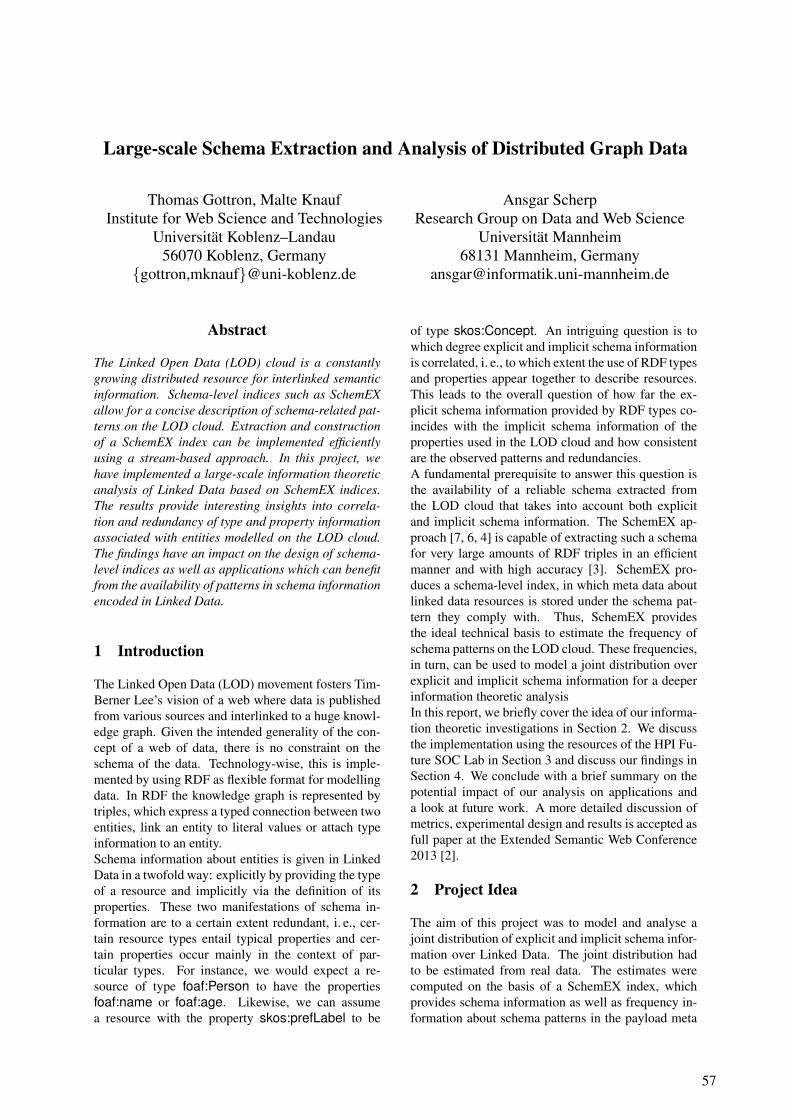
Large-scale Schema Extraction and Analysis of Distributed Graph Data

Thomas Gottron, Malte KnaufInstitute for Web Science and Technologies

Universitat Koblenz–Landau56070 Koblenz, Germany

{gottron,mknauf}@uni-koblenz.de

Ansgar ScherpResearch Group on Data and Web Science

Universitat Mannheim68131 Mannheim, Germany

[email protected]

Abstract

The Linked Open Data (LOD) cloud is a constantlygrowing distributed resource for interlinked semanticinformation. Schema-level indices such as SchemEXallow for a concise description of schema-related pat-terns on the LOD cloud. Extraction and constructionof a SchemEX index can be implemented efficientlyusing a stream-based approach. In this project, wehave implemented a large-scale information theoreticanalysis of Linked Data based on SchemEX indices.The results provide interesting insights into correla-tion and redundancy of type and property informationassociated with entities modelled on the LOD cloud.The findings have an impact on the design of schema-level indices as well as applications which can benefitfrom the availability of patterns in schema informationencoded in Linked Data.

1 Introduction

The Linked Open Data (LOD) movement fosters Tim-Berner Lee’s vision of a web where data is publishedfrom various sources and interlinked to a huge knowl-edge graph. Given the intended generality of the con-cept of a web of data, there is no constraint on theschema of the data. Technology-wise, this is imple-mented by using RDF as flexible format for modellingdata. In RDF the knowledge graph is represented bytriples, which express a typed connection between twoentities, link an entity to literal values or attach typeinformation to an entity.Schema information about entities is given in LinkedData in a twofold way: explicitly by providing the typeof a resource and implicitly via the definition of itsproperties. These two manifestations of schema in-formation are to a certain extent redundant, i. e., cer-tain resource types entail typical properties and cer-tain properties occur mainly in the context of par-ticular types. For instance, we would expect a re-source of type foaf:Person to have the propertiesfoaf:name or foaf:age. Likewise, we can assumea resource with the property skos:prefLabel to be

of type skos:Concept. An intriguing question is towhich degree explicit and implicit schema informationis correlated, i. e., to which extent the use of RDF typesand properties appear together to describe resources.This leads to the overall question of how far the ex-plicit schema information provided by RDF types co-incides with the implicit schema information of theproperties used in the LOD cloud and how consistentare the observed patterns and redundancies.A fundamental prerequisite to answer this question isthe availability of a reliable schema extracted fromthe LOD cloud that takes into account both explicitand implicit schema information. The SchemEX ap-proach [7, 6, 4] is capable of extracting such a schemafor very large amounts of RDF triples in an efficientmanner and with high accuracy [3]. SchemEX pro-duces a schema-level index, in which meta data aboutlinked data resources is stored under the schema pat-tern they comply with. Thus, SchemEX providesthe ideal technical basis to estimate the frequency ofschema patterns on the LOD cloud. These frequencies,in turn, can be used to model a joint distribution overexplicit and implicit schema information for a deeperinformation theoretic analysisIn this report, we briefly cover the idea of our informa-tion theoretic investigations in Section 2. We discussthe implementation using the resources of the HPI Fu-ture SOC Lab in Section 3 and discuss our findings inSection 4. We conclude with a brief summary on thepotential impact of our analysis on applications anda look at future work. A more detailed discussion ofmetrics, experimental design and results is accepted asfull paper at the Extended Semantic Web Conference2013 [2].

2 Project Idea

The aim of this project was to model and analyse ajoint distribution of explicit and implicit schema infor-mation over Linked Data. The joint distribution hadto be estimated from real data. The estimates werecomputed on the basis of a SchemEX index, whichprovides schema information as well as frequency in-formation about schema patterns in the payload meta

57

data stored in the index.To be more specific, we estimated the probability ofan entity on the LOD cloud to be described by a set oftypes t and a set of properties r by:

p(t, r) =|x ∈ SchemEX(t, r)|

Nwhere N is the overall number of entities described inthe analysed data set and x ∈ SchemEX(t, r) denotesthe set of entities indexed in SchemEX with the speci-fied set of types and properties.To model the joint distribution of type sets and prop-erty sets, we introduce two random variables T andR over the power sets TS = P(Classes) and PS =P(Properties) of all possible class type and propertycombinations, respectively. The joint distribution ofthis two random variables is then defined as:

P (T = t, R = r) = p(t, r)

On the basis of this joint distribution, we defined sev-eral metrics for answering our questions about infor-mation content and redundancy on the LOD cloud:

Normalized Entropy of the Marginal Distributions.To answer the question of how much informationis encoded in the type sets or the property set ofan entity, we consider the entropy [10] of the twomarginal distributions of P (T,R):

H(T ) = −∑t∈TS

P (T = t) · lg (P (T = t))

H(R) = −∑r∈PS

P (R = r) · lg (P (R = r))

For reasons of comparability, we further normal-ize these values making use of the maximal en-tropy:

H0(T ) =H(T )

lg(|TS|)

H0(R) =H(R)

lg(|PS|)

Expected Conditional Entropy. In order to respondto the question of how much information is stillcontained in the properties, once we know thetypes of an entity (or vice versa) implies a condi-tional probability and, thus, a conditional entropy.To further aggregate values over all possible con-ditions, we use the expected conditional entropy.The conditional entropy of the properties, giventhe types is defined as:

H(R|T ) =∑t∈TS

P (T = t)H(R|T = t)

= −∑t∈TS

∑r∈PS

p(t, r) lg

(p(t, r)

P (T = t)

)

The conditional entropy of the types, given theproperties is defined analogously.

Normalized Mutual Information. To finally answerthe question of how far explicit and implicitschema information is redundant, we make useof mutual information (MI) [1]. MI is a met-ric to capture the joint information conveyed bytwo random variables and, thereby, to which de-gree they can explain each other. The MI ofexplicit and implicit schema information of theLOD cloud is defined as:

I(T,R) =∑r∈PS

∑t∈TS

p(t, r) lgp(t, r)

P (T = t) · P (R = r)

A normalization of MI to the interval [−1, 1] isgiven in [11] and involves the entropy of themarginal distributions of T and R. This normal-ization serves as a direct measure for redundancyand is defined as:

I0(T,R) =I(T,R)

min (H(T ), H(R))

3 Implementation

For our empirical analysis, we use the different seg-ments of the data set provided for the Billion TripleChallenge (BTC) 2012. The BTC data set has beencrawled from the web in a typical web spider fashionand contains about 1.44 billion triples. It is dividedinto five segments according to the set of URLs usedas seed for the crawling process: Rest, Datahub, DB-Pedia, Freebase and Timbl. Details about the differentparts and the crawling strategies used for collecting thedata are described on the BTC 2012 data set’s web-site1.We consider especially the larger data segments partic-ularly useful as they span different aspects of the LODcloud. With Datahub, we have got a sample of severalpublicly available linked RDF data sources registeredin a central location. DBpedia is interesting as it isone of the central and most connected resources in theLOD cloud extracted from the collaboratively curatedWikipedia. Freebase, instead, is also a collaborativeknowledge base, but here the users directly operate onthe structural data. The Timbl data set is a crawl start-ing at the FOAF profile of Tim Berners-Lee (thus, thename). Hence, it provides a snapshot from yet a dif-ferent part of the LOD cloud, namely starting at small,manually maintained RDF files.We used resources from the HPI cluster to be able toperform the memory intensive computation of the met-rics in Section 2. We mainly made use of the Hewlett

1BTC 2012 data set: http://km.aifb.kit.edu/projects/btc-2012/

58

Packard DL980 G7 machines with 1 and 2 TB ofRAM. While we used the machines also for the extrac-tion of the schema-level index structures, the main mo-tivation for making use of HPI lab resources was theinformation theoretic analysis. Estimating a joint dis-tribution of type sets and property sets requires manag-ing a relatively fine grained decomposition of the datasets. Essential functionalities for the computation ofthe information theoretic measures are a fast and flexi-ble aggregation of the elements of this decomposition,which can easily be implemented in main memory.

4 Results

In this section we summarize the findings of our analy-sis. Table 1 gives an overview of the computed metricson the five segments of the BTC 2012 data set. We willnow go into the details of the single metrics.

Entropy in Type and Property Sets. We can ob-serve the tendency that the property sets convey moreinformation than type sets. This can be observed inthe higher values of the normalized entropies. For in-stance, the normalized marginal entropy of the prop-erty sets has a value of 0.324 on the DBpedia data set,while the normalized marginal entropy of the type setsis 0.093. This observation provides a hint that on DB-pedia the distribution into type sets is far more skewedthan the distribution of property sets. Similar obser-vations can be made for the data sets Rest, Freebaseand Timbl as well, though to a lower extent. An ex-ception is the Datahub data set, where the distributionof entities in type sets and property sets seems morecomparable.

Expected Conditional Entropies. Looking at theexpected conditional entropies reveals some interest-ing insights. Recall that the aggregation we chose forthe conditional entropy provides us with the expectedentropy, given a certain type set or property set. Wecan see in Table 1 that the entropy given a property settends to be far lower than the one when given a typeset. In conclusion: knowing the properties of an en-tity in these cases already tells us a lot about the entity,as the entropy of the conditional distribution can be ex-pected to be quite low. On the contrary, when knowingthe type of an entity, the entropy of the distribution ofthe property sets can be expected to be still relativelyhigh (when compared to the entropy of the marginaldistribution). We looked at the data more closely to in-vestigate how often a given type set is already a clearindicator for the set of properties (and vice versa). Themost extreme case is the Freebase data set, where for80.89% of all entities it is sufficient to know the set ofproperties in order to conclude the set of types asso-ciated with this entity. Knowing, instead, the types ofan entity conveys less information: only in 2.05% ofthe cases this is sufficient to precisely predict the set of

properties of an entity. Again, and with the exceptionof Datahub, the other data sets exhibit a similar trend.

Mutual Information. Finally, the value of the nor-malized MI gives us insights on how much one infor-mation (either properties or types) explains the respec-tive other. Also here, we observe a quite wide rangefrom 0.635 on DBpedia to 0.881 on Rest. Accordingly,extracting only type or only property information fromLOD can already explain a quite large share of the con-tained information. However, given our observations asignificant part of the schema information is encodedalso in the respective other part. The degree of this ad-ditional information depends on the part of the LODcloud considered. As a rule of thumb, we hypothesisethat collaborative approaches without a guideline fora schema (such as DBpedia) tend to be less redundantthan data with a narrow domain (Timbl) or some weakschema structure (Freebase).

Discussion of the Results. The observations on thelarge data sets provide us with insights into the formand structure of schema information on the LODcloud. First of all, the distribution of type sets andproperty sets tend to have a relatively high normalizedentropy. We can conclude that the structure of the datais not dominated by a few combinations of types orproperties. Accordingly for the extraction of schemainformation, we cannot reduce the schema to a smalland fixed structure but need to consider a wider vari-ety of type and property information. Otherwise theschema would loose too much information.

A second observation is the dependency between typesand properties. The conditional entropy reveals thatthe properties of an entity usually tell much moreabout its type than the other way around. This ob-servation is interesting for various applications. Forinstance, suggesting a data engineer the types of anentity based on the already modelled properties seemsquite promising [8]. We assume that this observationcan also be seen as an evidence that property infor-mation on the LOD cloud actually considers implicitor explicit agreements about the domain and range ofthe according property. However, this observation isnot valid for the entire LOD cloud. Depending on theconcrete setting and use case, a specific analysis mightneed to be run.

Finally, the observed MI values underline the varianceof schema information in the LOD cloud. Ranges from63.5% to 88.1% redundancy between the type sets andproperty sets have been observed. Thus, approachesbuilding a schema only over one of these two types ofschema information run at the risk of a significant lossof information.

59

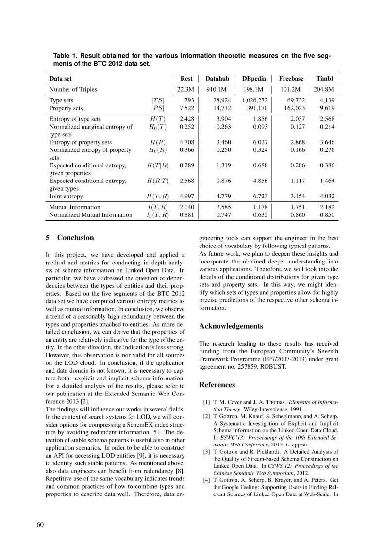
Table 1. Result obtained for the various information theoretic measures on the five seg-ments of the BTC 2012 data set.

Data set Rest Datahub DBpedia Freebase Timbl

Number of Triples 22.3M 910.1M 198.1M 101.2M 204.8M

Type sets |TS| 793 28,924 1,026,272 69,732 4,139Property sets |PS| 7,522 14,712 391,170 162,023 9,619

Entropy of type sets H(T ) 2.428 3.904 1.856 2.037 2.568Normalized marginal entropy oftype sets

H0(T ) 0.252 0.263 0.093 0.127 0.214

Entropy of property sets H(R) 4.708 3.460 6.027 2.868 3.646Normalized entropy of propertysets

H0(R) 0.366 0.250 0.324 0.166 0.276

Expected conditional entropy,given properties

H(T |R) 0.289 1.319 0.688 0.286 0.386

Expected conditional entropy,given types

H(R|T ) 2.568 0.876 4.856 1.117 1.464

Joint entropy H(T,R) 4.997 4.779 6.723 3.154 4.032

Mutual Information I(T,R) 2.140 2.585 1.178 1.751 2.182Normalized Mutual Information I0(T,R) 0.881 0.747 0.635 0.860 0.850

5 Conclusion

In this project, we have developed and applied amethod and metrics for conducting in depth analy-sis of schema information on Linked Open Data. Inparticular, we have addressed the question of depen-dencies between the types of entities and their prop-erties. Based on the five segments of the BTC 2012data set we have computed various entropy metrics aswell as mutual information. In conclusion, we observea trend of a reasonably high redundancy between thetypes and properties attached to entities. As more de-tailed conclusion, we can derive that the properties ofan entity are relatively indicative for the type of the en-tity. In the other direction, the indication is less strong.However, this observation is nor valid for all sourceson the LOD cloud. In conclusion, if the applicationand data domain is not known, it is necessary to cap-ture both: explicit and implicit schema information.For a detailed analysis of the results, please refer toour publication at the Extended Semantic Web Con-ference 2013 [2].The findings will influence our works in several fields.In the context of search systems for LOD, we will con-sider options for compressing a SchemEX index struc-ture by avoiding redundant information [5]. The de-tection of stable schema patterns is useful also in otherapplication scenarios. In order to be able to constructan API for accessing LOD entities [9], it is necessaryto identify such stable patterns. As mentioned above,also data engineers can benefit from redundancy [8].Repetitive use of the same vocabulary indicates trendsand common practices of how to combine types andproperties to describe data well. Therefore, data en-

gineering tools can support the engineer in the bestchoice of vocabulary by following typical patterns.As future work, we plan to deepen these insights andincorporate the obtained deeper understanding intovarious applications. Therefore, we will look into thedetails of the conditional distributions for given typesets and property sets. In this way, we might iden-tify which sets of types and properties allow for highlyprecise predictions of the respective other schema in-formation.

Acknowledgements

The research leading to these results has receivedfunding from the European Community’s SeventhFramework Programme (FP7/2007-2013) under grantagreement no. 257859, ROBUST.

References

[1] T. M. Cover and J. A. Thomas. Elements of Informa-tion Theory. Wiley-Interscience, 1991.

[2] T. Gottron, M. Knauf, S. Scheglmann, and A. Scherp.A Systematic Investigation of Explicit and ImplicitSchema Information on the Linked Open Data Cloud.In ESWC’13: Proceedings of the 10th Extended Se-mantic Web Conference, 2013. to appear.

[3] T. Gottron and R. Pickhardt. A Detailed Analysis ofthe Quality of Stream-based Schema Construction onLinked Open Data. In CSWS’12: Proceedings of theChinese Semantic Web Symposium, 2012.

[4] T. Gottron, A. Scherp, B. Krayer, and A. Peters. Getthe Google Feeling: Supporting Users in Finding Rel-evant Sources of Linked Open Data at Web-Scale. In

60

Semantic Web Challenge, Submission to the BillionTriple Track, 2012.

[5] T. Gottron, A. Scherp, B. Krayer, and A. Peters. LO-Datio: Using a Schema-Based Index to Support Usersin Finding Relevant Sources of Linked Data. In K-CAP’13: Proceedings of the Conference on Knowl-edge Capture, 2013. to appear.

[6] M. Konrath, T. Gottron, and A. Scherp. Schemex –web-scale indexed schema extraction of linked opendata. In Semantic Web Challenge, Submission to theBillion Triple Track, 2011.

[7] M. Konrath, T. Gottron, S. Staab, and A. Scherp.SchemEX—Efficient Construction of a Data Cata-logue by Stream-based Indexing of Linked Data. WebSemantics: Science, Services and Agents on the WorldWide Web, 16(5):52 – 58, 2012. The Semantic WebChallenge 2011.

[8] J. Schaible, T. Gottron, S. Scheglmann, and A. Scherp.LOVER: Support for Modeling Data Using LinkedOpen Vocabularies. In LWDM’13: 3rd InternationalWorkshop on Linked Web Data Management, pages89–92, 2013.

[9] S. Scheglmann, G. Groner, S. Staab, and R. Lammel.Incompleteness-aware programming with rdf data. InE. Viegas, K. Breitman, and J. Bishop, editors, Pro-ceedings of the 2013 Workshop on Data Driven Func-tional Programming, DDFP 2013, Rome, Italy, Jan-uary 22, 2013, pages 11–14. ACM, 2013.

[10] C. Shannon. A mathematical theory of communica-tion. Bell System Technical Journal, 27:379–423 and623–656, July and October 1948.

[11] Y. Y. Yao. Information-theoretic measures for knowl-edge discovery and data mining. In J. K. Karmeshu,editor, Entropy Measures, Maximum Entropy Prin-ciple and Emerging Applications, pages 115–136.Springer, Berlin, 2003.

61

Storage Class Memory Evaluation for SAP HANA

Ahmadshah Waizy [email protected]

Dieter Kasper [email protected]

Konrad Büker [email protected]

Karsten Beins [email protected]

Jürgen Schrage [email protected]

Fujitsu Technology Solutions GmbH Heinz-Nixdorf-Ring 1

33106 Paderborn, Germany

Bernhard Höppner [email protected]

Felix Salfner [email protected]

Henning Schmitz [email protected]

Joos-Hendrik Böse [email protected]

SAP Innovation Center Potsdam Prof.-Dr.-Helmert-Str. 2-3 14482 Potsdam, Germany

Abstract

Storage Class Memory (SCM) introduces a new stor-age technology, which combines word granular ac-cess by single CPU instructions with the advantage of being non-volatile and offering a high storage density. It is well suited to increase the memory ca-pabilities of individual servers efficiently to deal with increasing memory demands of applications and can also be used to store data permanently. SCM technology could potentially be utilized in many software applications. We concentrate on the in-memory computing database SAP HANA, which may particularly benefit from the introduction of SCM technology. Several possible applications of the new technology are analyzed. As SCM prototypes are not yet available physically we have developed a soft-ware emulator to simulate the effects of a physical presence of SCM technology on the speed of data access. This simulation is then used as the basis for extensive benchmarking of one field of application. The results of those benchmarks are presented in this document. This project was executed at the Future SOC Lab of the Hasso-Plattner-Institute in Potsdam (Berlin), Germany. It utilized a Fujitsu RX600 server with 1 TB RAM, which is part of the lab’s infrastructure.

1 Introduction

In existing architectures a clear distinction between memory and storage is made when developing soft-

ware. Hard disk (HDD) or solid-state disk (SSD) based storage offers non-volatile characteristics and high storage density leading to low prices. By con-trast, memory technologies like dynamic random access memory (DRAM) offer low latencies and byte granular access. This distinction leads main decision in software architectures. Introducing the SCM tech-nology might be an inflection point for today’s para-digms. SCM combines the characteristics of memory and storage, offering low latencies and byte granular access as well as high storage density and being non-volatile. SAP’s in-memory computing appliance SAP HANA introduces a technology that can be used to address problems in the domain of real-time processing of big data [1]. It may profit of the mentioned advantages in multiple ways. In general two different approaches are possible. The non-volatile characteristic of SCM offers new ways to ensure the durability of data whereas low latencies make SCM interesting for in-memory databases in order to work directly on the data utilizing a higher storage density compared to DRAM. Therefore it is particularly interesting to investigate how SAP HANA could benefit from the introduction of SCM and what adoptions might be needed to enable SAP HANA to use SCM. This report summarizes the findings of the “Storage Class Memory Evaluation for SAP HANA” and documents its results. In summary we have

• Provided a description of the SCM technol-ogy characteristics and how it is simulatedusing an emulator.

63

• Conducted a capability study to determinesome applications in which using SCMmight be particularly rewarding.

• Benchmarked the characteristics of SCM byusing I/O processing, SAP HANA basedevent stream processing, and a SAP specificbenchmark from the domain of EnterpriseResource Planning applications based onSAP HANA, the so-called SD benchmark.

• Discussed the next steps this project shouldtake as regards enabling SAP HANA to uti-lize SCM most efficiently.

2 Storage Class Memory Technology

Emerging device technologies including phase change-memory (PCM), spin-torque transfer RAM (STT-RAM) and memristors promise high-speed storage. These technologies collectively are termed storage-class memory (SCM) as data can be accessed through ordinary load/store instructions rather than through I/O requests. Hence, user-mode code can access data directly, so there is no need for the oper-ating system to mediate every access. The availability of large persistent memory combined with a small lowering of access speed seems to be within reach in the next 3-5 years. This is likely to trigger a new software design for applications, mid-dleware and operating systems. Being prepared for this revolutionary step is the request of this research, with a special view on SAP HANA. The software architectures as we know them (operat-ing system as well as applications and data bases) are built on a foundation of fast volatile memory and slow persistent storage. The difference in latency between “fast” (memory) and “slow” (storage) lies in the order of magnitude of factor 106.

Figure 1: Access characteristics of different types of data storage media

With the introduction of flash memory the gap be-tween “fast” and “slow” became somewhat smaller, see Figure 1. But still, flash memory acts as storage block device, because the granularity is given by physical limitations shown in Figure 2:

• Page_size: Size of the smallest atomic reador write operation (approx. 4k on enterpriseSingle-Level Cell, SLC and 32k on consum-er Multi-Level Cell, MLC).

• Segment_size: Size of the smallest atomicerase operation (approx. 64k on enterpriseSLC, 4m on consumer MLC).

Upcoming SCM technologies are technologies which will allow the CPU a more fine granular access by word as it is used today with DDR (Double Data Rate), see mark in Figure 2. This combination of real word granularity access by a single CPU instruction in combination with persistency and a large afforda-ble capacity bigger than DRAM upturns the existing software architecture.

Figure 2: Extended memory / storage hier-archy layers considering SCM

The characteristics of this new technology are essen-tially the fine granular access of data by Byte/Word, the accessibility by a single CPU instruction, the non-volatility, relatively low access times, the higher density than DRAM, and lower cost per bit.

3 Capability Study

Introducing Storage Class Memory as an inflection point for software architectures leads to the need for developing approaches to leverage the technology. Today’s solutions make a clear distinction between the usage of non-volatile storage with a rather low performance but high data density and volatile memory with a high performance but low data densi-ty. This distinction has an impact on many decisions when designing software. With a view to SAP HANA this explains the usage of main memory for all actively used data in order to provide real time transactional and analytical operations. To ensure the durability of data, non-volatile storage is used to keep savepoints and log files. The following chapters focus on two main topics on how to use SCM in a future database application. In general we divide our attempts by the properties of SCM. At first we make use of the non-volatility characteristic of SCM by suggesting approaches for data persistence. Next we take a closer look onto the high data density and low latencies by introducing use cases for data aging and

64

a so-called Scale-In idea. We present general strate-gies on how to address the features of SCM and give first insights into their implementation efforts. We also evaluate those strategies by explaining their benefits and possible drawbacks.

3.1 Storage Class Memory for Data Persis-tence

The data persistence layer of a database is responsi-ble for assuring that no data is lost if the system crashes and that the last consistent state is restored after the system has been repaired. Data persistence usually consists of two major parts, which are data checkpoints (sometimes also called savepoints or snapshots) and a transaction log that persists all committed changes to the database after the last checkpoint has been saved. In case of a database recovery, the last checkpoint is loaded into the data-base first. The transaction log is replayed thereafter so that the database is brought back into the last con-sistent state that was saved before the crash. The need to save snapshots and transaction logs to persistent storage is a requirement also for in-memory databases. Although the data is kept in main memory, the database must be able to restore the last consistent state in case of, e.g., a power failure. SCM being non-volatile has - at least - the potential to survive power failures. However, writing to second-ary storage such as flash disks, and shipping it to some redundant file server still offers a significantly higher level of fault tolerance. Therefore writing persistent data onto local SCM will not be sufficient from a fault-tolerance point of view. Fault-tolerant storage will be discussed in the next section. Never-theless, SCM offers word-access to the data. We investigated how this could improve the data persis-tency layer of an in-memory database.

3.1.1 Transactional Logging SCM offers increased access speed and the ability to support addressing of single data words, which is not offered by today’s persistence layers - HDD and flash-based IO devices operate on a block-level only. We investigated whether this specific advantage could improve transactional logging of in-memory-databases significantly. Access at word granularity level is beneficial pri-marily for scenarios with random data access pat-terns, i.e., data is either read or written in arbitrary patterns or data is read or written randomly to arbi-trary positions of the device. Unfortunately, the log-ging layer of data persistency does not show any of these characteristics. Logging usually is a process where data is simply appended to the end of the log. During recovery, data is primarily read sequentially from storage. As SCM offers about equal throughput for large data transfers if compared to contemporary block-oriented storage, we do not see high potential in using SCM to significantly improve transactional

logging. Only in the case of a high number of very short transactions SCM could outperform traditional solutions. However, massive changes concerning the persistence layer of an existing database would be necessary to implement a fine granular logging whereas advantages might only be feasible for a small subset of transactions.

3.1.2 Redundancy The same arguments hold for the redundancy part of the data persistence layer of databases. Writing snap-shots primarily forms a sequential data access pattern so that data word access does not provide significant benefit. This is at least true for contemporary data-base persistency layers, which are optimized for HDD-based storage tiers. To better exploit the per-formance of SCM efficiently for database persistence layers new data structures and approaches are re-quired. Some promising approach could be a more or less direct mapping of HANAs in-memory data structures to SCM. A first candidate for such a strategy could be the delta store, which is manipulated by every write operation. Using random word level access of SCM would allow keeping a complete copy of the delta store on SCM storage and recovering using a simple copy of the SCM structure to RAM. Therefore the need of transactional logging for the delta store would vanish and the persistence of the delta store could be achieved by memory copy instructions. Also this results in additional effort in redesigning the persistence layer but the performance increase is theoretically very promising.

3.2 Storage Class Memory for Data Aging and Scale-In

Companies face an enormously increasing amount of data being stored in their systems today. For new retail customers at SAP this could mean an average growth of 40GB per month in the first year [3]. Even when using an in-memory computing database like SAP HANA this fact leads to the problems of

• An increasing demand of memory, whichleads to the infeasibility of keeping the en-tire data in main memory.

• A decreasing performance given by increas-ing processing times of database operations.

Figure 3 illustrates the correlation of database table fill levels and resulting database query response times. A decreasing performance can especially be observed for increasing fill levels regarding scan and aggregate operations where large datasets need to be processed. In the following we will discuss ideas on how to overcome the mentioned issues. Our main driving force is given by the fact that today’s busi-ness store data of the last ten years on average, while only 20% are used actively [1].

65

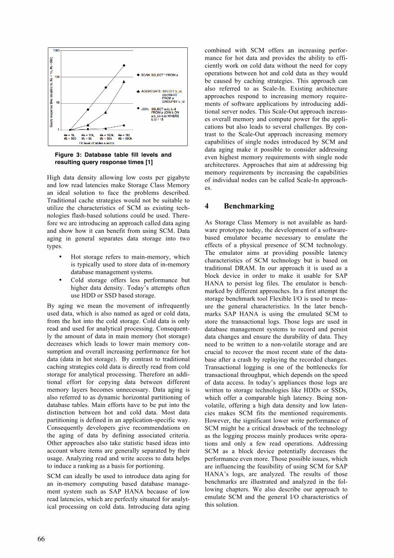
Figure 3: Database table fill levels and resulting query response times [1]

High data density allowing low costs per gigabyte and low read latencies make Storage Class Memory an ideal solution to face the problems described. Traditional cache strategies would not be suitable to utilize the characteristics of SCM as existing tech-nologies flash-based solutions could be used. There-fore we are introducing an approach called data aging and show how it can benefit from using SCM. Data aging in general separates data storage into two types.

• Hot storage refers to main-memory, whichis typically used to store data of in-memorydatabase management systems.

• Cold storage offers less performance buthigher data density. Today’s attempts oftenuse HDD or SSD based storage.

By aging we mean the movement of infrequently used data, which is also named as aged or cold data, from the hot into the cold storage. Cold data is only read and used for analytical processing. Consequent-ly the amount of data in main memory (hot storage) decreases which leads to lower main memory con-sumption and overall increasing performance for hot data (data in hot storage). By contrast to traditional caching strategies cold data is directly read from cold storage for analytical processing. Therefore an addi-tional effort for copying data between different memory layers becomes unnecessary. Data aging is also referred to as dynamic horizontal partitioning of database tables. Main efforts have to be put into the distinction between hot and cold data. Most data partitioning is defined in an application-specific way. Consequently developers give recommendations on the aging of data by defining associated criteria. Other approaches also take statistic based ideas into account where items are generally separated by their usage. Analyzing read and write access to data helps to induce a ranking as a basis for portioning. SCM can ideally be used to introduce data aging for an in-memory computing based database manage-ment system such as SAP HANA because of low read latencies, which are perfectly situated for analyt-ical processing on cold data. Introducing data aging

combined with SCM offers an increasing perfor-mance for hot data and provides the ability to effi-ciently work on cold data without the need for copy operations between hot and cold data as they would be caused by caching strategies. This approach can also referred to as Scale-In. Existing architecture approaches respond to increasing memory require-ments of software applications by introducing addi-tional server nodes. This Scale-Out approach increas-es overall memory and compute power for the appli-cations but also leads to several challenges. By con-trast to the Scale-Out approach increasing memory capabilities of single nodes introduced by SCM and data aging make it possible to consider addressing even highest memory requirements with single node architectures. Approaches that aim at addressing big memory requirements by increasing the capabilities of individual nodes can be called Scale-In approach-es.

4 Benchmarking

As Storage Class Memory is not available as hard-ware prototype today, the development of a software-based emulator became necessary to emulate the effects of a physical presence of SCM technology. The emulator aims at providing possible latency characteristics of SCM technology but is based on traditional DRAM. In our approach it is used as a block device in order to make it usable for SAP HANA to persist log files. The emulator is bench-marked by different approaches. In a first attempt the storage benchmark tool Flexible I/O is used to meas-ure the general characteristics. In the later bench-marks SAP HANA is using the emulated SCM to store the transactional logs. Those logs are used in database management systems to record and persist data changes and ensure the durability of data. They need to be written to a non-volatile storage and are crucial to recover the most recent state of the data-base after a crash by replaying the recorded changes. Transactional logging is one of the bottlenecks for transactional throughput, which depends on the speed of data access. In today’s appliances those logs are written to storage technologies like HDDs or SSDs, which offer a comparable high latency. Being non-volatile, offering a high data density and low laten-cies makes SCM fits the mentioned requirements. However, the significant lower write performance of SCM might be a critical drawback of the technology as the logging process mainly produces write opera-tions and only a few read operations. Addressing SCM as a block device potentially decreases the performance even more. Those possible issues, which are influencing the feasibility of using SCM for SAP HANA’s logs, are analyzed. The results of those benchmarks are illustrated and analyzed in the fol-lowing chapters. We also describe our approach to emulate SCM and the general I/O characteristics of this solution.

66

4.1 Storage Class Memory Emulator SCM is a step towards a fundamentally new memory hierarchy with deep implications across the soft-ware/hardware interface. Our emulator is implemented as a block device driver for Linux that simulates the presence of a SCM in-stalled in one of the DIMM slots on the motherboard. The emulator is implemented as a kernel module for Linux that creates “/dev/scm0” when it is loaded and which acts as a block device with SCM latencies lying on top of the RAM device. Figure 4 shows the implementation concept. When the module is loaded, it benchmarks the performance of the systems RAM and computes the differences between the latencies of the RAM-disk and the simulated SCM. All read/write operations into the RAM-disk will be emulated with latencies of the SCM. Since the SCM technology will come with different read/write latency values, the emulator provides a command called “scmadm”, which allows to individ-ually configure the latency factors for read and write operations. So the emulator is capable of simulating a SCM with different latency values.

Figure 4: Emulator concept as a RAM-disk backed by a kernel block device driver

The emulator is a Linux RAM-disk driver which adds the wanted latency factors to SCM access. The emu-lated SCM latencies (delay factors for reading and writing) can be adjusted after the SCM driver is load-ed by using the emulator command “scmadm”. Fig-ure 5 explains the implemented interfaces.

Figure 5: Emulator Interfaces

From a number of published SCM references (e.g. [4] to [11]) we extracted various delay times for writing and for reading operations. Figure 6 lists the latencies being predicted in publications. Our emulated SCM test cases are focusing on SCM_Ref_1 and SCM_Ref_2. (PCRAM = Phase Change Random Access Memory).

Figure 6: Expected read/write latencies ex-tracted from publications

In order to compare the access behavior of a DRAM with the one of an emulated SCM, we carried out measurements with test pattern derived from the map depicted in Figure 7. In the map the contour of the triangle comprises the area of expected SCM laten-cies, once SCM is available.

The triangle is derived from the SCM characteristics given in Figure 6: Using the fact that reading will always be faster than writing, and assuming that SCM read/write will be always slower than DRAM read/write, and based on our given real system DRAM latencies as the starting point P5=(80ns;80ns), the contour of the triangle was esti-mated considering SCM_Ref_1 and SCM_Ref_2 to be positioned in the center area of the triangle.

Name Mode DRAM PCRAM ReRAM STT-RAMSCM_Ref_1 read 60 ns 300 ns -- --

write 60 ns 700 ns -- --SCM_Ref_2 read 60 ns 300 ns -- --

write 60 ns 1400 ns -- --Ref_3 read 55 ns 48 ns 100 ns 1.96 ns

write 55 ns 150 ns 100 ns 7.76 nsRef_4 read 10-60 ns 48 ns <10 ns <10 ns

write 10-60 ns 40-150 ns ~10 ns 12.5 nsRef_5 read -- 70 ns 7.2 ns 11 ns

write -- >180 ns <7.2 ns 25 nsRef_6 read -- 10-100 ns -- --

write -- 100-1000 ns -- --Ref_7 read -- -- 1.773 - 426.8 ns --

write -- -- 100.6 - 518.2 ns --Ref_8 read 70 ns 206 ns -- --

write 70 ns 7100 ns -- --

67

Figure 7: Expected range of SCM latencies considered towards emulation

From the triangle the test points listed in Figure 8 have been chosen.

Figure 8: Chosen test points

In the emulator a test point can be applied by setting a specific read/write delay factor using the “scmadm” command. The following sections describe tests with the synthetic program “fio” and tests with a real SAP HANA which both have been carried out using the test point parameters listed in Figure 8.

4.2 Flexible I/O Tester (fio) The “fio” is an I/O tool meant to be used for both, benchmarking and stress/hardware verification. It can work on block devices as well as on files. The “fio” accepts job descriptions in a text format. We used the block device “fio” test according to the following description:

[global] bs=4k direct=1, numjobs=1 ioengine=libaio, iodepth=2 iodepth_batch=1, iodepth_batch_complete=0 rw=randwrite/randread, use_os_rand=1 randrepeat=0, time_based runtime=30, [job]filename=/dev/scm0 size=1GB

Figure 9 presents reading-test results with read laten-cies of 80/160/320/400/560 ns. The order of the curves corresponds to the order of latencies used.

Figure 9: IOPS for different read latencies

Figure 10 presents writing-test results with write latencies of 80/400/560/720/880/1360/1920 ns. The order of the curves corresponds to the order of the latencies used.

Figure 10: IOPS for different write latencies

From Figure 11 we can conclude that latency has an exponential-like impact on IOPS. Latencies larger than 750 ns bring IOPS dramatically down.

Figure 11: Impact on IOPS by different emu-lated latencies

Test point read [ns] write [ns]SCM_Ref_1 320 720SCM_Ref_2 320 1360

P3 560 560P4 320 400P5 80 80P6 160 880P7 320 1920P8 400 1360

SCM emulated test points

68

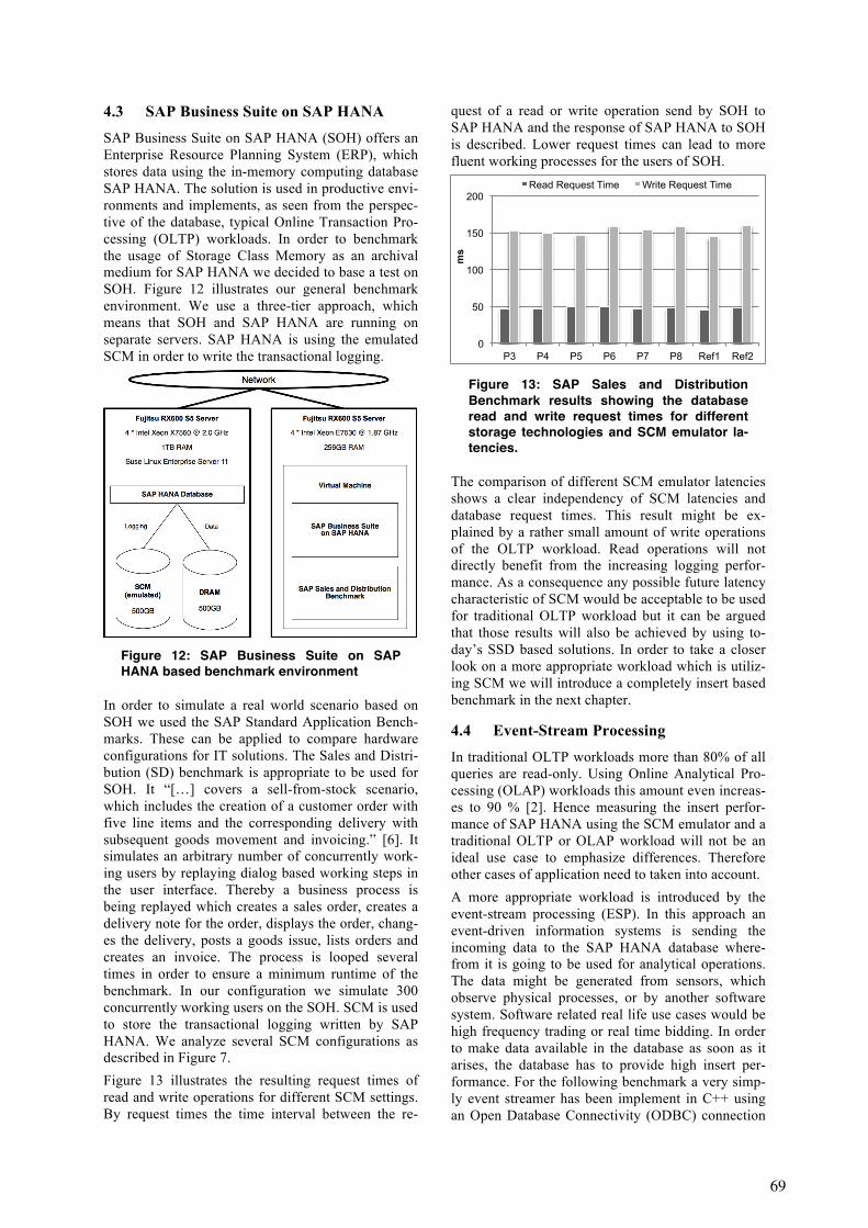
4.3 SAP Business Suite on SAP HANA SAP Business Suite on SAP HANA (SOH) offers an Enterprise Resource Planning System (ERP), which stores data using the in-memory computing database SAP HANA. The solution is used in productive envi-ronments and implements, as seen from the perspec-tive of the database, typical Online Transaction Pro-cessing (OLTP) workloads. In order to benchmark the usage of Storage Class Memory as an archival medium for SAP HANA we decided to base a test on SOH. Figure 12 illustrates our general benchmark environment. We use a three-tier approach, which means that SOH and SAP HANA are running on separate servers. SAP HANA is using the emulated SCM in order to write the transactional logging.

Figure 12: SAP Business Suite on SAP HANA based benchmark environment

In order to simulate a real world scenario based on SOH we used the SAP Standard Application Bench-marks. These can be applied to compare hardware configurations for IT solutions. The Sales and Distri-bution (SD) benchmark is appropriate to be used for SOH. It “[…] covers a sell-from-stock scenario, which includes the creation of a customer order with five line items and the corresponding delivery with subsequent goods movement and invoicing.” [6]. It simulates an arbitrary number of concurrently work-ing users by replaying dialog based working steps in the user interface. Thereby a business process is being replayed which creates a sales order, creates a delivery note for the order, displays the order, chang-es the delivery, posts a goods issue, lists orders and creates an invoice. The process is looped several times in order to ensure a minimum runtime of the benchmark. In our configuration we simulate 300 concurrently working users on the SOH. SCM is used to store the transactional logging written by SAP HANA. We analyze several SCM configurations as described in Figure 7. Figure 13 illustrates the resulting request times of read and write operations for different SCM settings. By request times the time interval between the re-

quest of a read or write operation send by SOH to SAP HANA and the response of SAP HANA to SOH is described. Lower request times can lead to more fluent working processes for the users of SOH.

Figure 13: SAP Sales and Distribution Benchmark results showing the database read and write request times for different storage technologies and SCM emulator la-tencies.

The comparison of different SCM emulator latencies shows a clear independency of SCM latencies and database request times. This result might be ex-plained by a rather small amount of write operations of the OLTP workload. Read operations will not directly benefit from the increasing logging perfor-mance. As a consequence any possible future latency characteristic of SCM would be acceptable to be used for traditional OLTP workload but it can be argued that those results will also be achieved by using to-day’s SSD based solutions. In order to take a closer look on a more appropriate workload which is utiliz-ing SCM we will introduce a completely insert based benchmark in the next chapter.

4.4 Event-Stream Processing In traditional OLTP workloads more than 80% of all queries are read-only. Using Online Analytical Pro-cessing (OLAP) workloads this amount even increas-es to 90 % [2]. Hence measuring the insert perfor-mance of SAP HANA using the SCM emulator and a traditional OLTP or OLAP workload will not be an ideal use case to emphasize differences. Therefore other cases of application need to taken into account. A more appropriate workload is introduced by the event-stream processing (ESP). In this approach an event-driven information systems is sending the incoming data to the SAP HANA database where-from it is going to be used for analytical operations. The data might be generated from sensors, which observe physical processes, or by another software system. Software related real life use cases would be high frequency trading or real time bidding. In order to make data available in the database as soon as it arises, the database has to provide high insert per-formance. For the following benchmark a very simp-ly event streamer has been implement in C++ using an Open Database Connectivity (ODBC) connection

0

50

100

150

200

P3 P4 P5 P6 P7 P8 Ref1 Ref2

ms

Read Request Time Write Request Time

69

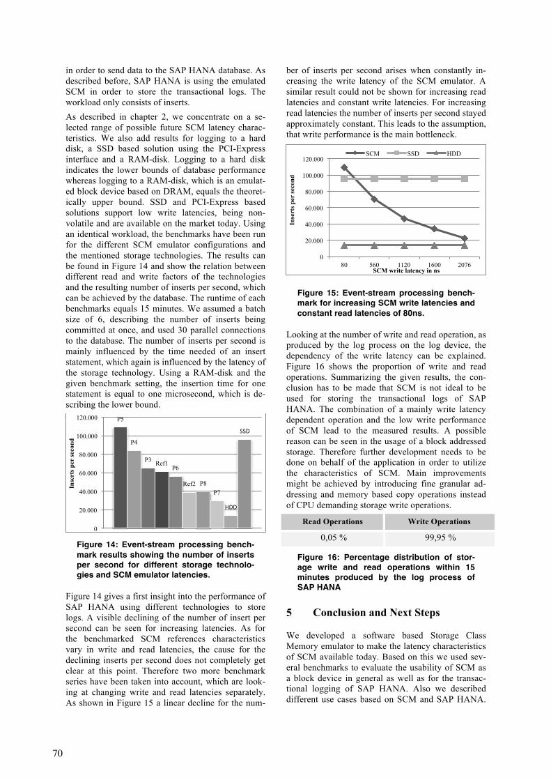
in order to send data to the SAP HANA database. As described before, SAP HANA is using the emulated SCM in order to store the transactional logs. The workload only consists of inserts. As described in chapter 2, we concentrate on a se-lected range of possible future SCM latency charac-teristics. We also add results for logging to a hard disk, a SSD based solution using the PCI-Express interface and a RAM-disk. Logging to a hard disk indicates the lower bounds of database performance whereas logging to a RAM-disk, which is an emulat-ed block device based on DRAM, equals the theoret-ically upper bound. SSD and PCI-Express based solutions support low write latencies, being non-volatile and are available on the market today. Using an identical workload, the benchmarks have been run for the different SCM emulator configurations and the mentioned storage technologies. The results can be found in Figure 14 and show the relation between different read and write factors of the technologies and the resulting number of inserts per second, which can be achieved by the database. The runtime of each benchmarks equals 15 minutes. We assumed a batch size of 6, describing the number of inserts being committed at once, and used 30 parallel connections to the database. The number of inserts per second is mainly influenced by the time needed of an insert statement, which again is influenced by the latency of the storage technology. Using a RAM-disk and the given benchmark setting, the insertion time for one statement is equal to one microsecond, which is de-scribing the lower bound.

Figure 14: Event-stream processing bench-mark results showing the number of inserts per second for different storage technolo-gies and SCM emulator latencies.

Figure 14 gives a first insight into the performance of SAP HANA using different technologies to store logs. A visible declining of the number of insert per second can be seen for increasing latencies. As for the benchmarked SCM references characteristics vary in write and read latencies, the cause for the declining inserts per second does not completely get clear at this point. Therefore two more benchmark series have been taken into account, which are look-ing at changing write and read latencies separately. As shown in Figure 15 a linear decline for the num-

ber of inserts per second arises when constantly in-creasing the write latency of the SCM emulator. A similar result could not be shown for increasing read latencies and constant write latencies. For increasing read latencies the number of inserts per second stayed approximately constant. This leads to the assumption, that write performance is the main bottleneck.

Figure 15: Event-stream processing bench-mark for increasing SCM write latencies and constant read latencies of 80ns.

Looking at the number of write and read operation, as produced by the log process on the log device, the dependency of the write latency can be explained. Figure 16 shows the proportion of write and read operations. Summarizing the given results, the con-clusion has to be made that SCM is not ideal to be used for storing the transactional logs of SAP HANA. The combination of a mainly write latency dependent operation and the low write performance of SCM lead to the measured results. A possible reason can be seen in the usage of a block addressed storage. Therefore further development needs to be done on behalf of the application in order to utilize the characteristics of SCM. Main improvements might be achieved by introducing fine granular ad-dressing and memory based copy operations instead of CPU demanding storage write operations.

Read Operations Write Operations

0,05 % 99,95 %

Figure 16: Percentage distribution of stor-age write and read operations within 15 minutes produced by the log process of SAP HANA

5 Conclusion and Next Steps

We developed a software based Storage Class Memory emulator to make the latency characteristics of SCM available today. Based on this we used sev-eral benchmarks to evaluate the usability of SCM as a block device in general as well as for the transac-tional logging of SAP HANA. Also we described different use cases based on SCM and SAP HANA.

P5

P4

P3 Ref1 P6

Ref2 P8 P7

HDD

SSD

0

20.000

40.000

60.000

80.000

100.000

120.000

Inse

rts p

er se

cond

0

20.000

40.000

60.000

80.000

100.000

120.000

80 560 1120 1600 2076

Inse

rts p

er se

cond

SCM write latency in ns

SCM SSD HDD

70

Looking at the benchmark results we can emphasize that using SCM as a block device is beneficial for latencies lower than 150ns but the resulting perfor-mance can only slightly outperform today’s solu-tions. Taking the word addressability of SCM into account might be crucial to achieve even better re-sults. Therefore decisive changes have to be made to the existing application in order to utilize the tech-nology. In a next step we will take a closer look at the performance of SAP HANA using SCM to store the in-memory data. Additionally, we will investigate if the technology is suitable for use cases like data aging.

References [1] Hasso Plattner, Alexander Zeier: In-Memory Data

Management: An Inflection Point for Enterprise Ap-plications, Springer, 2011.

[2] Jens Krüger, Changkyu Kim, Martin Grund, Nadathur Satish, David Schwalb, Jatin Chhugani, Hasso Platt-ner, Pradeep Dubey, Alexander Zeier. Fast Updates on Read-Optimized Databases Using Multi-Core CPUs. Proceedings of the VLDB Endowment, 5 (1):61–72, 2011.

[3] SAP AG. Data Management Guide for SAP Business Suite, 2006.

[4] X. Dong, Y. Xie, “Modeling and Leveraging Emerg-ing Non-Volatile Memories for Future Computer De-signs”, Submitted to ACM Student Research Competi-tion, Department of Computer Science and Engineer-ing, Pennsylvania State University, USA, 2011.

[5] S. Lee, B. Moon, C. Park, J.Y. Hwang, and K. Kim, "Accelerating In-Page Logging with Non-Volatile Memory", presented at IEEE Data Engineering, Bulle-tin, 2010, pp.41-47.

[6] C. Mohan, S. Bhattacharya, “Implications of Storage Class Memories (SCM) on Software Architectures”, Presentation at workshop on the use of Emerging Storage and Memory Technologies (WEST), HPCA 2010, Bangalore, India, January 2010.

[7] D. A. Roberts, “Efficient Data Center Architectures Using Non-Volatile Memory and ReliabilityTech-niques”, Dissertation, Computer Science and Engi-neering, University of Michigan, USA, 2011.

[8] T. Perez, C. De Rose, “Non-Volatile Memory: Emerg-ing Technologies And Their Impacts on Memory Sys-tems”, Technical Report Nº 060, Pontifícia Univer-sidade Católica do Rio Grande do Sul; Faculdade de Informática Pós-Graduação em Ciência da Computação, Porto Alegere, Brasil, September 2010.

[9] Y. Xie, “Emerging NVM Memory Technologies”, Presentation, Department of Computer Science and Engineering, Pennsylvania State University, USA, 2010.

[10] C. Xu, X. Dong e.a., “Design Implications of Memris-tor-Based RRAM Cross-Point Structures”, Proceed-ings Design, Automation and Test in Europe Confer-ence DATE 2011, Grenoble, France, March 2011.

[11] J. Grollier, “Memristors”, Presentation at NANO-TEC Workshop 2 - Benchmarking of new Beyond CMOS device/design concepts, Athens, Greece, October 2011.

[12] SAP AG. SAP Standard Application Benchmarks. Sales and Distribution. http://www.sap.com /campaigns/benchmark/appbm_sd.epx. Accessed: 21/03/2013.

71

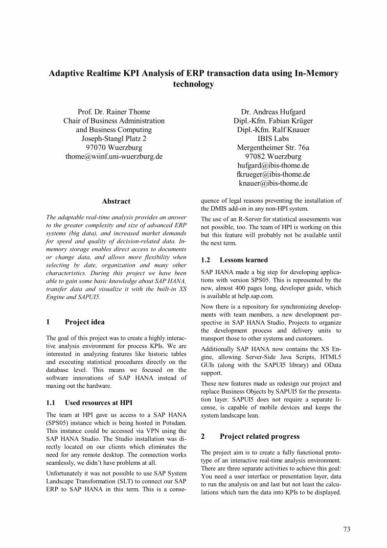
Adaptive Realtime KPI Analysis of ERP transaction data using In-Memory technology

Prof. Dr. Rainer Thome Chair of Business Administration

and Business Computing Joseph-Stangl Platz 2

97070 Wuerzburg [email protected]

Dr. Andreas Hufgard Dipl.-Kfm. Fabian Krüger Dipl.-Kfm. Ralf Knauer

IBIS Labs Mergentheimer Str. 76a

97082 Wuerzburg [email protected] [email protected] [email protected]

Abstract

The adaptable real-time analysis provides an answer to the greater complexity and size of advanced ERP systems (big data), and increased market demands for speed and quality of decision-related data. In-memory storage enables direct access to documents or change data, and allows more flexibility when selecting by date, organization and many other characteristics. During this project we have been able to gain some basic knowledge about SAP HANA, transfer data and visualize it with the built-in XS Engine and SAPUI5.

1 Project idea

The goal of this project was to create a highly interac-tive analysis environment for process KPIs. We are interested in analyzing features like historic tables and executing statistical procedures directly on the database level. This means we focused on the software innovations of SAP HANA instead of maxing out the hardware.

1.1 Used resources at HPI The team at HPI gave us access to a SAP HANA (SPS05) instance which is being hosted in Potsdam. This instance could be accessed via VPN using the SAP HANA Studio. The Studio installation was di-rectly located on our clients which eliminates the need for any remote desktop. The connection works seamlessly, we didn’t have problems at all. Unfortunately it was not possible to use SAP System Landscape Transformation (SLT) to connect our SAP ERP to SAP HANA in this term. This is a conse-

quence of legal reasons preventing the installation of the DMIS add-on in any non-HPI system. The use of an R-Server for statistical assessments was not possible, too. The team of HPI is working on this but this feature will probably not be available until the next term.

1.2 Lessons learned SAP HANA made a big step for developing applica-tions with version SPS05. This is represented by the new, almost 400 pages long, developer guide, which is available at help.sap.com. Now there is a repository for synchronizing develop-ments with team members, a new development per-spective in SAP HANA Studio, Projects to organize the development process and delivery units to transport those to other systems and customers. Additionally SAP HANA now contains the XS En-gine, allowing Server-Side Java Scripts, HTML5 GUIs (along with the SAPUI5 library) and OData support. These new features made us redesign our project and replace Business Objects by SAPUI5 for the presenta-tion layer. SAPUI5 does not require a separate li-cense, is capable of mobile devices and keeps the system landscape lean.

2 Project related progress

The project aim is to create a fully functional proto-type of an interactive real-time analysis environment. There are three separate activities to achieve this goal: You need a user interface or presentation layer, data to run the analysis on and last but not least the calcu-lations which turn the data into KPIs to be displayed.

73

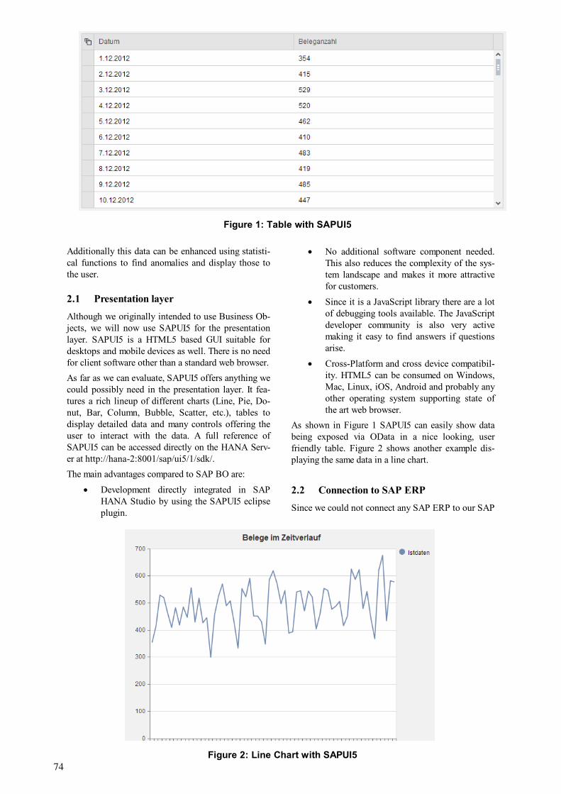
Additionally this data can be enhanced using statisti-cal functions to find anomalies and display those to the user.

2.1 Presentation layer Although we originally intended to use Business Ob-jects, we will now use SAPUI5 for the presentation layer. SAPUI5 is a HTML5 based GUI suitable for desktops and mobile devices as well. There is no need for client software other than a standard web browser. As far as we can evaluate, SAPUI5 offers anything we could possibly need in the presentation layer. It fea-tures a rich lineup of different charts (Line, Pie, Do-nut, Bar, Column, Bubble, Scatter, etc.), tables to display detailed data and many controls offering the user to interact with the data. A full reference of SAPUI5 can be accessed directly on the HANA Serv-er at http://hana-2:8001/sap/ui5/1/sdk/. The main advantages compared to SAP BO are:

• Development directly integrated in SAPHANA Studio by using the SAPUI5 eclipseplugin.

• No additional software component needed.This also reduces the complexity of the sys-tem landscape and makes it more attractivefor customers.

• Since it is a JavaScript library there are a lotof debugging tools available. The JavaScriptdeveloper community is also very activemaking it easy to find answers if questionsarise.

• Cross-Platform and cross device compatibil-ity. HTML5 can be consumed on Windows,Mac, Linux, iOS, Android and probably anyother operating system supporting state ofthe art web browser.

As shown in Figure 1 SAPUI5 can easily show data being exposed via OData in a nice looking, user friendly table. Figure 2 shows another example dis-playing the same data in a line chart.

2.2 Connection to SAP ERP Since we could not connect any SAP ERP to our SAP

Figure 1: Table with SAPUI5

Figure 2: Line Chart with SAPUI5 74

HANA instance, we still had to rely on sample data. This data has been extracted from an IDES System into .csv files and then imported into SAP HANA using the “Import from local file” feature in SAP HANA Studio. It is suitable for testing some queries but does not change over time. That’s why we simu-lated a time series and used this data for the presenta-tion layer. From a technical point of view it does not matter if the data is from a simulation or an SQL-Script actually calculating the real number of open orders per day. Once there is real-time data available the data source can be exchanged easily.

2.3 KPI Calculations As presented in the last report, we already have some procedures calculating the open sales orders for any user-defined date in the past. The only change in KPI calculation is that we can now store our procedures in the repository using “.procedure” files. On Activa-tion, these Design-Time files create the stored proce-dures (Run-Time). One of the main advantages of those Design-Time .procedure-Files is the ability to debug them. You can set breakpoints, run the proce-dure and the debugger will stop on every breakpoint, allowing you to see the contents of any variable. You can also control which parts of the code were actually executed and which were not when using if-clauses or loops. Other than this technical change, due to the new re-

lease, there have been no changes to the KPI calcula-tion.

2.4 Statistical integration In the beginning we thought SAP HANA would na-tively support the statistical programming language R since you could define procedures and set the lan-guage to “RLang”. Unfortunately it turns out that SAP HANA does not process these procedures itself but sends it to another server with an R installation as well as the plugin RServ. All the statistical computa-tions are then executed on the R server and then sent back to SAP HANA. This is a massive drawback since a potential customer would need another server in his landscape, this server would also need a fast CPU and a lot of RAM, and it would have to be set up and maintained separately. Nevertheless we developed an R procedure which computes the weekday of the date and executes a lin-ear regression on the documents, explaining the num-ber of documents as function of a constant, a general linear trend and the weekday. Using this regression results, R can even predict the next few days and cal-culate a lower and upper confidence limit. Since the integration between SAP HANA and R was not possible this term we were able to test it locally. Using RStudio and the sample data as seen in figure 1 and 2 we get the output seen in figure 3. The red line shows the actual data which ends on

Dez 01 Dez 15 Jan 01 Jan 15 Feb 01

020

040

060

0

Date

Doc

umen

ts

Figure 3: Dynamic Thresholds with R

75

February 1. Using this data R computes the purple (upper limit) and green (lower limit) lines. The background of this is that some KPIs show natu-ral fluctuation within a week. For example, open or-ders might be higher on Mondays since customers order products on the weekend but nobody is working to process them. On the other hand, open orders should dramatically reduce until Friday because oth-erwise the customers would have to wait the whole weekend. Therefore you need different thresholds depending on factors like the weekday. Since R integration with SAP HANA involves some problems with extra hardware, we are currently ana-lyzing the brand new PAL (Predictive Analysis Li-brary) functionality from SPS05. This library also offers statistical functions but those can be executed natively by the SAP HANA instance itself. Maybe this can reduce the complexity of the application.

3 Further research

Until now we have already proven that SAP HANA has all capabilities to enable the interactive reporting we looked for. All of the layers (presentation, calcula-tion, and statistics) are working as separate parts, but to make this application fully functional there are some tasks left:

• The data source is still missing. SAP nowoffers the whole SAP Business Suite onHANA. This eliminates the need for SLT orother replication tools. A high quality datasource is needed for testing the time travelqueries.

• Until now we only have looked into the openorders. There are similar ones like blocked,cancelled and completed orders and somewhich need to be calculated differently like‘changed orders’.

• We already eliminated Business Objects asan external dependency by using SAPUI5.

• R integration is still a problem but couldpossibly be replaced by PAL.

• All the different layers need to be connectedto each other and integrated. If there are mul-tiple GUI elements (like tables and charts),they should respond to selections, sendthose as filters to the HANA server and thenupdate the other elements as well. On theother hand it would be nice to have somekind of push notification for the user if thecurrent KPI value is out of the control limits.

76

Application Aware Placement and Scheduling for Multi-tenant Clouds

Lalith Suresh1 and Marco Canini2

1Technische Universitat Berlin, Germany2Universite Catholique de Louvain, Belgium

{[email protected], [email protected]}

Abstract

In an Infrastructure-as-a-Service (IaaS) environment,it is paramount to perform intelligent allocation ofshared resources. Placement is the problem of choos-ing which virtual machine (VM) should run on whichphysical machine (PM), whereas Scheduling is theproblem of sharing resources between multiple co-located VMs. An efficient placement and schedulingis one, that in addition to satisfying all constraints,increases the overall utilization of physical resourcessuch as CPU, storage, or network. Determining anefficient placement and scheduling is a very challeng-ing problem, especially in face of conflicting goals andpartially available information about workloads.In order to reason about placement, we first tackle theproblem of performance interference that may affectco-located VMs—when there is more demand by mul-tiple VMs for a resource than is available at a giveninstant of time. We thus characterize the performanceof Hadoop in a shared and virtualized setting.

1 Introduction

The focus of our study is multi-tenant, multi-purposeInfrastructure-as-a-Service (IaaS) cloud data centers,wherein servers are virtualized, with multiple tenantsdeploying applications atop shared infrastructure. Uti-lizing compute, storage and network resources effi-ciently is a crucial objective in these environmentsas virtual machines (VMs) are collocated on physicalservers and contend for a set of shared resources onthe physical server and network.However, it is well-known that virtualized comput-ing environments can suffer from performance inter-ference (see e.g., [4]). More precisely, due to imper-fect performance isolation by the underlying hyper-visors and lack of fine-grained bandwidth assurancesacross tenants within the network, the performance of

a VM may suffer due to collocated VMs. Such per-formance interference can lead to unpredictable delaysfor the cloud tenant, which would ultimately manifestin failed service-level agreements (SLAs) at the appli-cation level and in loss of business revenue.

To mitigate performance interference, it is thus im-portant to balance the different workloads of varioustenants across the data center. While VMs from dif-ferent tenants may be collocated on the same physi-cal host, different tenants in the data center may havevarying demands for resources depending on the ap-plications that they are running. For instance, a tenantrunning a Hadoop [3] deployment on the cloud mayhave a greater demand for disk I/O bandwidth than atenant managing a multi-tier website. Depending onthe resource demands of different applications beingrun by different tenants, VMs may experience varyingdegrees of performance interference due to contentionfor shared resources. Thus, the performance degrada-tion experienced by different VMs is sensitive to thespecific placement of VMs in the data center [7].

Since this performance degradation depends on the ap-plications being run within the VMs, understandinghow applications behave and where their bottlenecksare may allow an operator to perform smarter place-ment of VMs within the data center. This projecttakes a fresh look at the fundamental problem ofapplication placement in the private cloud environ-ment. Application placement is the task of decid-ing which VM runs on which physical server. Therehave been proposals to address application placementfrom both theoretical and systems standpoints. Forinstance, theoretical approaches model the environ-ment as a multi-dimensional bin packing problem [8]or provide schedules based on statistical models [1].However, these models are too coarse to accuratelyaccount for performance interference, which requirefine-grained experimentation to observe. On the otherhand, [5, 6, 2, 9] propose techniques to identify per-formance interference by observing low-level system

77

metrics on individual VMs and then making placementdecisions to minimize it or allocating more resourcesto compensate for interference. However, these ap-proaches do not exploit the specific characteristics andgoals of the applications.In fact, in today’s cloud ecosystem, most applica-tions are distributed across more than one VM. Withservice-oriented architectures becoming the norm,systems are decomposed into multiple, loosely cou-pled, communicating clusters of components. An in-dividual logical component in an application could byitself be a self-healing system comprised of multiplenodes, which have built-in mechanisms to compen-sate for stragglers or slower nodes (e.g, MapReduce’sscheduler). Taking these aspects into consideration,we argue that performance interference should be rea-soned about at the granularity of logical componentsof the application using application-specific metrics,and not at the granularity of the individual VMs usingsystem-level metrics. This project aims to demonstratethis fact experimentally.In order to design application- and interference-awareapproaches to plan application placement in multi-tenant clouds, we first try to characterize the perfor-mance of different systems under multi-tenant envi-ronments. This information can then be used to ef-fectively place applications in a cloud, as show in themethodology illustrated in Figure 1. In the findingspresented below, we present performance results ofrunning Hadoop in shared environments.

2 Usage of Future SOC Lab

HPI FSOC Lab provided us access to a state-of-the art,1000-core computing cluster. The cluster consists of25 nodes, each equipped with 40 cores at 2.40 GHz,1 TB RAM, 3.6 TB SSD storage and 10 Gbps Ether-net. To use this cluster for our experimental study, weneeded it to be configured as a virtualized cloud en-vironment, and we obtained simultaneous, dedicatedaccess to all nodes.We ran experiments of the Hadoop cluster under mul-tiple configurations and co-location scenarios.

• Baseline: every VM of the Hadoop cluster is run-ning on a separate physical machine.

• Co-located Datanodes: two Hadoop DatanodeVMs from the same cluster are co-located eachphysical machines.

• Co-located Clusters: a VM each from two differ-ent Hadoop clusters are co-located on the samephysical machine.

Through our runs, we vary the number of reducersused by Hadoop, the Hadoop scheduler being used(Capacity and Fair schedulers), and we enable/disablespeculative execution (wherein tasks are speculatively

cloned to account for stragglers). We use the follow-ing notations to describe the combinations of these pa-rameters. cpt and cpf represent the use of the Capac-ity Scheduler along with speculative execution enabledand disabled, respectively. fst and fsf represent the useof the Fair Scheduler along with speculative executionenabled and disabled, respectively. The workload werun is the TeraSort benchmark that is packaged withthe Hadoop distribution, with four jobs submitted inparallel.

3 Findings

In this section, we describe some of our findings.Figure 2 represents measurements of the differencebetween the maximum and minimum job completiontimes when submitting four TeraSort jobs to the clusterat the same time, under varying scenarios. We use thisas an indication of fairness in the system. We find thatthe baseline and co-located Datanodes scenarios pro-vide identical fairness when using different schedulersand regardless of whether speculative execution is en-abled or disabled. However, in the co-located clustersscenario, we observe that due to performance inter-ference from each cluster on the other, the system isunable to guarantee fairness in job completion timeseven when using the Hadoop Fair Scheduler. Figure 3describes the same set of results but when using 10 re-ducers instead of 1. Since Hadoop can now distributethe reduce tasks over multiple nodes, the skew in jobcompletion times is minimized, but still remains sig-nificant in the co-located clusters scenario.One challenge we faced in obtaining more results andmeasurements was that the specifications of the phys-ical machines being used deviated significantly fromthose used in typical Infrastructure-as-a-Service de-ployments, where servers have a different CPU coresto I/O bandwidth ratio.

4 Summary and Future Work

Our studies indicate that performance interference notonly affects the job completion times of Hadoop di-rectly, but also leads to interference in the Hadoopschedulers, affecting the guarantees they are expectedto provide (such as fairness). We plan to use thesemeasurements in order to prepare measurement-driveninterference models which can in turn be used as in-put to placement algorithms which can be used to mapVMs to physical machines in cloud environments. Ourstudy will also extend to other systems such as key-value stores and the interactions between these sys-tems.

5 Acknowledgements

We would like to thank the system administrators ofthe Future SOC-Lab infrastructure for their support, in

78

DeployApplication

Causal PathAnalysis

OnlineSandboxingand Offline

Analysis

Overlay Graph

Baseline Profile+

Resource Profile+

Interference Matrix

InterferenceMinimizingPlacement

1

2

3

4

5

6

VirtualMachines

Figure 1: At a high level, our workflow combines online and offline measurements of ap-plications with specific i nformation a bout t he a pplication’s i nternals i n o rder t o perform interference minimizing placement.

particular with setting up OpenStack on the machines.We also thank Zubair Khwaja Sediqi for help with thesetup of the measurement code and workloads.

References

[1] R. C. Chiang and H. H. Huang. Tracon: interference-aware scheduling for data-intensive applications in vir-tualized environments. In Proc. ACM SC, 2011.

[2] D. Novakovic et al. Deepdive: Transparently identify-ing and managing performance interference in virtual-ized environments. In Proc. USENIX ATC, 2013.

[3] A. Hadoop. http://hadoop.apache.org/, lastaccessed Dec 20th, 2013.

[4] Y. Koh, R. Knauerhase, P. Brett, M. Bowman, Z. Wen,and C. Pu. An analysis of performance interference ef-fects in virtual environments. In Performance Analysisof Systems & Software, 2007. ISPASS 2007. IEEE Inter-national Symposium on, pages 200–209. IEEE, 2007.

[5] Y. Koh, R. Knauerhase, P. Brett, M. Bowman, Z. Wen,and C. Pu. An analysis of performance interference ef-fects in virtual environments. In Proc. IEEE ISPASS,2007.

[6] R. Nathuji, A. Kansal, and A. Ghaffarkhah. Q-clouds:managing performance interference effects for qos-aware clouds. In Proc. EuroSys, 2010.

[7] A. Roytman, A. Kansal, S. Govindan, J. Liu, andS. Nath. Algorithm design for performance aware vmconsolidation.

[8] B. Urgaonkar, A. Rosenberg, and P. Shenoy. Applica-tion placement on a cluster of servers. Int. J. Found.Comput. Sci., 2007.

[9] Y. Xu, Z. Musgrave, B. Noble, and M. Bailey. Bobtail:avoiding long tails in the cloud. In Proc. NSDI, 2013.

79

● ●

●

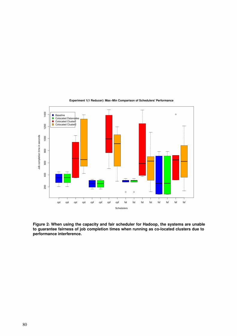
cpt cpt cpt cpt cpf cpf cpf cpf fst fst fst fst fsf fsf fsf fsf

200

400

600

800

1000

1200

1400

Experiment 1(1 Reducer): Max−Min Comparison of Schedulers' Performance

Schedulers

Job

com

plet

ion

time

in s

econ

ds

Baseline Colocated DatanodesColocated Cluster1Colocated Cluster2

Figure 2: When using the capacity and fair scheduler for Hadoop, the systems are unable to guarantee fairness of job completion times when running as co-located clusters due to performance interference.

80

●

● ●

●

●

● ●

●

●

●

●

●

●

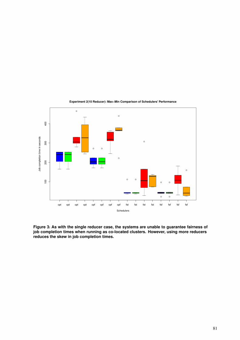
cpt cpt cpt cpt cpf cpf cpf cpf fst fst fst fst fsf fsf fsf fsf

100

200

300

400

Experiment 2(10 Reducer): Max−Min Comparison of Schedulers' Performance

Schedulers

Job

com

plet

ion

time

in s

econ

ds

Figure 3: As with the single reducer case, the systems are unable to guarantee fairness of job completion times when running as co-located clusters. However, using more reducers reduces the skew in job completion times.

81

A framework for comparing the performance of in-memory and traditional

disk-based databases

Vassilena Banova

Technische Universität München

Chair for Information Systems

Boltzmannstr. 3, 85748 Garching, Germany

[email protected]

Alexandru Danciu




[email protected]

Helmut Krcmar




[email protected]

Abstract

Enterprises are facing an increasing amount of data,

and rely more than ever on flexible and fast methods

of data analysis. A proposed solution is the switch to

in-memory database systems which promise huge

performance increases. Unfortunately recent litera-

ture does not provide performance comparisons of

main-memory and classical storage based database

systems in enterprise use cases. A literature review is

conducted identifying the scenario of discovering

frequent item-sets as an appropriate use case to

perform such a comparison. Requirements on a test

environment are provided and a tool supporting

those tests is implemented, encouraging the execution

of OLAP, OLTP and mixed workload test-suites.

1 Introduction

Today’s enterprises store and collect more data than

ever. It is estimated that the fortune 500 enterprises

store approximately seven to ten years of customer

data [1]. This amount is told to increase even further

in the coming years [2]. Amongst others this data is

used in the context of Business Intelligence & Ana-

lytics“(BI&A) to gain insights on the market and

make critical decisions in a timely manner based on

up to date information [3]. But the huge amount of

data makes it necessary to narrow the data down or to

work with pre-calculated results what limits the flex-

ibility and expressiveness of the analysis [4]. In an

environment of fast changing market conditions and

customer wishes this flexibility is crucial to recog-

nize influences on the own business and react on

undesirable developments [2].

A frequently used term in this context is “Big Data”

what describes the processing and analysis of huge

amounts of data with complex structure [3] and is

sometimes referred to as a scaled BI&A [5]. The

properties of Big Data, “high-volume, high-variety,

high-velocity, and high-veracity“[6], often referred to

as the three “HVs” [6], make it necessary for enter-

prises to come up with new requirements on storage,

management, analysis and visualization of data [3].

One proposed solution to deal with these require-

ments is the use of in-memory databases, which de-

scribe database systems holding the entire dataset in

main memory [7]. A study conducted amongst Ger-

man IT-professionals in 2012, pointed out that every

fifth enterprise thinks that meeting the challenges of

the future data volume is only possible using in-

memory technology. But the same study pointed out,

that 60% of the enterprises are not able to make a

clear decision on whether in-memory databases are

relevant to them. They are especially concerned

whether the proposed advantages of in-memory tech-

nology can really be leveraged in their enterprise [2].

To achieve a better understanding about the effects of

in-memory databases and to be able to make a sound

decision on whether to invest into in-memory tech-

nology and migrate from traditional disk-based stor-

age to main memory storage, enterprises need tests to

be executed, comparing those technologies in enter-

prise use cases and providing insights on basic char-

acteristics of the database systems. Those tests will

help enterprises to determine the most suitable set up

for their needs. This project aims on developing some

basic test cases and the necessary toolset for execut-

ing this kind of tests.

83


2.1 Project Description

The project aims at the development of a testing

environment for the comparison of response times of

in-memory based and classical disk storage databases

in enterprise use case scenarios.

Two identical virtual machines, one with an in-

memory database system, the other with a classical

disk based storage database are used to verify, that

the developed test cases can be executed on such

environments. Therefore the same dataset is deployed

to both virtual machines. Queries are generated and

executed from a third, independent, source where

response time is measured. The target is to provide a

test setup including enterprise use cases being able to

compare two database systems.

2.2 Project Phases

In a first phase a literature review on database per-

formance and benchmarks was conducted to identify

relevant stakeholders, use cases and requirements for

testing. During this literature review four major

groups of stakeholders and their major topics of in-

terest could be identified. The four groups, consisting

of database developers, database administrators,

business analysts and end-user/decision makers were

characterized and the assumption was made, that the

group of business analysts is the most appro-priate

target group and that scenarios in data mining such as

the identification of frequent item-sets or the

measurement of profits and losses generated by a

specific sales-channel and its components are appro-

priate use cases for testing. Furthermore the absence

of tests comparing an in-memory database to a clas-

sical disk storage database in a comprehensible, re-

producible way and on equal conditions could be

approved.

In a second phase a framework for plan execution

was developed simulating different circumstances for

the virtual machines. The framework focuses on

varying three components in the test environment -

namely the number of threads executing one query in

parallel, the size of the dataset and plans of execu-

tion, determining whether update and select state-

ments are executed irrespective of each other or not.

The number of threads and the different datasets

represent the different amount of users and size of an

enterprise. Different plans of execution allow a com-

parison of the databases for different areas of applica-

tion. This increases the expandability of the tool to

further application domains and aims on evaluating

performance in mixed OLTP (Online Transaction

Processing) and OLAP (Online analytical Pro-

cessing) workloads.

In a third phase appropriate datasets were generated

and queries for testing were developed. Furthermore

a tool was implemented to execute the tests and

measure response time on both virtual machines on

equal conditions.

Data is extracted from the publicly available data

generator of the TPC-DS benchmark, an industry

standard benchmark for decision support systems

(see: www.tpc.org), as it is available for free and

approved to provide appropriate data for performance

testing. For reasons of simplification only two of

those tables were used. “catalog_sales” and “cata-

log_returns” which provide a fact table of sales

through the catalog sales channel including items and

orders and the profit and loss information of each line

item. This information, in combination with the page

number of the catalog, the item was ordered from,

allows to execute the aforementioned business use

cases. The tool for query execution is written in Java

and uses JDBC to send the chosen queries to the

databases and measure their response time.

3 Description of the Virtual Machines

The virtual machines provided by the HPI Future

SOC Lab both had 64 GB main memory, a hard drive

disk with a capacity of 100 GB and a total of eight

CPUs available. They are both located in the same

network and run a Linux Kernel 2.6.32.59-0.7.

4 Test-framework and Toolset

4.1 Requirements

The test-framework is supposed to provide decision

support for enterprises when deciding on switching to

or adding an in-memory database to their IT land-

scape. Therefore the framework for testing has to

simulate several environmental scenarios/enterprise

characteristics and provide details about the influ-

ences on performance if those environmental factors

change. As a test environment will never exactly

match a real enterprise, metrics of comparison should

be expressed in relative numbers and an easy, com-

prehensible way such as “On a level playing field, an

increase of users by factor x performance loss of

system A is factor z and performance loss of system

B is factor y - B runs r times faster than A”.

Another important factor for generating an as equal

as possible setup of the two databases, is to forbid

every kind of tuning, such as additional indexes.

Methods or elementary approaches as parts of the

database management system can be used. Therefore

tuning mechanisms such as adding further indexes to

a table have to be avoided. Using a columnar table

layout is appropriate. Basically the databases are

supposed to be used in out-of-the-box versions as

extra tuning might not be available for both database

instances the same way and the test is not supposed

to compare different tuning mechanisms.

Queries are supposed to be expressed in a way, that

both database systems can handle the same expres-

84

sion as good as possible. Furthermore the queries

have to be repeatable and comprehensible and have

to be logged or generated in a way that reproduction

is explicit.

The combination of queries and workload should try

to emphasize the differences in the database systems

and should therefore be designed to point out

strengths and weaknesses of both instances.

The measurement of response time may not include

the time necessary for query generation or the writing

of result-sets. Therefore the machine running the test

tool shall not be changed during tests and only the

execution time of the SQL Statement is to be meas-

ured.

4.2 Design of tests

Environmental Factors

To meet the above mentioned requirements for simu-

lating environmental factors the Queries are supposed

to be executed by {1, 5, 10, 20, 40} Threads in paral-

lel on a catalog_sales table of sizes {5GB, 10GB,

20GB, 40GB, 60GB, 80GB}. Those values were

chosen as they can be computed in a relatively mod-

erate time and are based on almost constant growth-

rate. The high volumes of data are selected as they

are close to (60GB) or even above (80GB) the avail-

able main memory (64GB).

In addition to the catalog_sales table the cata-

log_returns table is used with a constant size of 0.5

GB.

Queries

One test consists of six queries which can be grouped

into three categories. The first category consists of

queries which perform very basic and simple SQL

statements like selects or unions. The second group

of queries are either inserting lines or updating tables

and therefore represent OLTP workload. The third

group includes rather expensive queries including

joins and calculations.

It has to be mentioned, that the queries are not de-

signed to perform their tasks in the most efficient

way, but to generate workload on the database. The

six queries are:

- Insert lines: a specified number of Lines {1, 50,

-

-

-

100, 150, 200, 250} is inserted into the catalog

sales table at once. This query was chosen to

evaluate the write performance for a high num-

ber of columns.

Update one: this query updates one column in

the catalog_sales table for a specific collection of

items. This helps to evaluate update performance

of single column and creates OLTP workload.

Update six: this query updates six different

columns of the catalog sales table for a prede-

fined set of items. Here the update performance

of multiple columns is tested.

Select all: this statement simply returns the

whole catalog_sales table and gives insight about

the read performance of multiple columns.

-

-

-

Select distinct: this statement returns the distinct

values of item ids in the catalog_sales table and

therefore provides insights about the read per-

formance of a single column, what should be es-

pecially beneficial for a column store database.

Frequent item sets: this set of queries identifies

Items which occur together in different orders a

specific at least a predefined number of times.

Through the implementation using an increasing

number of self joins of the table catalog sales,

join performance and the power of the internal

query optimizer can be evaluated.

Profit loss per catalog page: this query calcu-

lates based on the catalog_sales and cata-

log_returns table which page of a catalog caused

which profit and what amount of loss. Here the

performance of calculation operations such as

sum() can be compared.

5 Test implementation

As mentioned before the tool suite was written in

Java and uses JDBC to connect to the different in-

stances. The architecture of the tool is rather simple,

as one Class “Executer” executes the whole test suite

by receiving Query-Strings of the “Generator” clas-

ses and starts the desired amount of threads “Run-

ners”.

Those threads can be executed in a variable and con-

figurable order and amount, allowing to generate a

mixed workload, too.

Response time is measured by storing the current

system time before executing a statement and imme-

diately after the result is received.

In the following, examples of the queries are provid-

ed and some difficulties identified are described.

Insert lines: For this query the disk storage database

and the in-memory database have to use different

SQL-statements. For the classical database the typi-

cal “insert into table values (val1),(val2)…” state-

ment is used. Unfortunately the tested in-memory

database is not able to process such a query with

more than one value. A workaround proposed, is to

write the query as “insert into table (Select value1

from dummy union all Select value2 from dummy

…). But this statement does not allow to insert more

than around 250 lines at a time as the query is then

told to be too complex to be processed. To avoid

primary key constraints, each thread accesses its own

file generated from one big TPC-DS catalog_sales

data file. After one iteration, when all threads have

finished, the data is deleted and the insert begins

again.

The update one query is defined as “Update cata-

log_sales Set cs_warehouse = {a randomly generated

integer of equal size for each Thread} where

cs_item_sk = {predefined value} OR cs_item_sk =

85

…”. The update six query is written accordingly but

sets five more columns {cs_ship_mode_sk,

cs_call_center_sk, cs_promo_sk, cs_ship_hdemo_sk,

cs_ship_cdemo_sk} to new values. Those columns

were chosen as they have no constraints and are not

used by any other query.

“Select * from catalog_sales” is the statement exe-

cuted by the select all statement and “Select distinct

cs_item_sk from catalog_sales” is the query behind

select distinct.

More interesting and causing a really heavy workload

on the database is query set for identifying frequent

itemsets.

The queries are generated by one thread executing

queries in the style of “Select cs1.cs_item_sk as

Item1, cs2.cs_item_sk as Item2 from catalog_sales

cs1 inner join catalog_sales cs2 on

cs1.cs_order_number = cs2.cs_order_number where

cs1.cs_item_sk < cs2.cs_item_sk AND group by

cs1.cs_item_sk, cs2.cs_item_sk having count

(cs1.cs_order_number) > {predefined value}” with

an increasing amount of items, until no result is re-

turned. Those queries are then stored in a list and

executed one another by the “Runner”. For each of

these queries the time is locked. Unfortunately, the

in-memory database stops when calculating itemsets

with three items, while the classical database exceeds

this number.

The profit loss per catalog page query is defined as:

“Select page_sk, sum (sales_price) as

sales_price_sum, sum(profit) as profit_sum,

sum(return_amt) as returns_sum , sum (net_loss) as

loss_sum From (select cs_catalog_page_sk as

page_sk, cs_sold_date_sk as

date_sk, cs_ext_sales_price as sales_price,

cs_net_profit as profit, cast(0 as decimal(7,2)) as

return_amt, cast(0 as decimal(7,2)) as net_loss

from catalog_sales

union all select cr_catalog_page_sk as page_sk, cr_returned_date_sk as date_sk, cast(0 as deci-

mal(7,2)) as sales_price, cast(0 as decimal(7,2)) as

profit, cr_return_amount as return_amt, cr_net_loss

as net_loss from catalog_returns ) group by

page_sk”. Here a number of calculation operations

are executed.

6 Project Outcome

6.1 Number of threads

The analysis shows that the DDB handles an increas-

ing number of threads better than the MMDB. The

query execution time increases slower with the DDB.

The impact of an increasing number of threads de-

pends for both databases on the data set size. With a

10 GB data set, an increasing number of threads has

more impact on the MMDB than on the DDB. With a

20 GB data set, the DDB is more susceptible to an

increasing number of threads.

Overall, the performed test showed that DBB per-

forms better with increasing number of threads. The

impact the number of threads has on the time dura-

tion a query rises with increasing data sets. However,

when increasing the size of the data set after 20 GB

the impact seems to be constant when increasing the

number of threads.

Regarding the predictability of time duration for

queries the DDB shows better results than the

MMDB irrespective of the size of the data set.

6.2 Size of dataset

With the 5 GB data set the MMDB outperformed the

DBB, particularly for complex queries and a high

number of threads.

For the 10 GB data set the DBB was superior to the

MMDB for all types of queries.

For the 20 GB data set the MMDB excels again, for

almost all types of queries.

The DBB performs best for ad-hoc queries, while the

MMDB is better for complex data mining queries.

An advantage of the MMDB for incremental sizes of

data sets is to be expected as here the gains of main

memory and column based storage have increased

impact. A verification with a 40 GB data set was for

reasons of time limitation not possible.

It can be seen that across all analyses the use of MQT

is a lot more efficient than the use of a view operat-

ing a MMDB.

The analysis of different types of queries could not

show any benefit using one or the other database.

6.3 Summary

ID Assumption Evalua-

tion

E 1.1 The impact on the average speed of

the queries for increasing number

of threads is smaller on a MMDB

than on a DDB

◔

E 1.2 With increasing size of the data set

the ability to operate many parallel

threads has a greater impact ◑

E 2.1 The time duration of a query execu-

tion is better predictable on MMDB

than DDB ○

E 3.1 The average query is faster on a

MMDB than a DDB ◑ E 3.2 For increasing size of data the

speed benefit increases ● E 4.1 Query properties can be matched to

database categories to enlarge or

diminish the advantages / down-

sides

◔

Table 1: Assumptions and their fulfillment

86

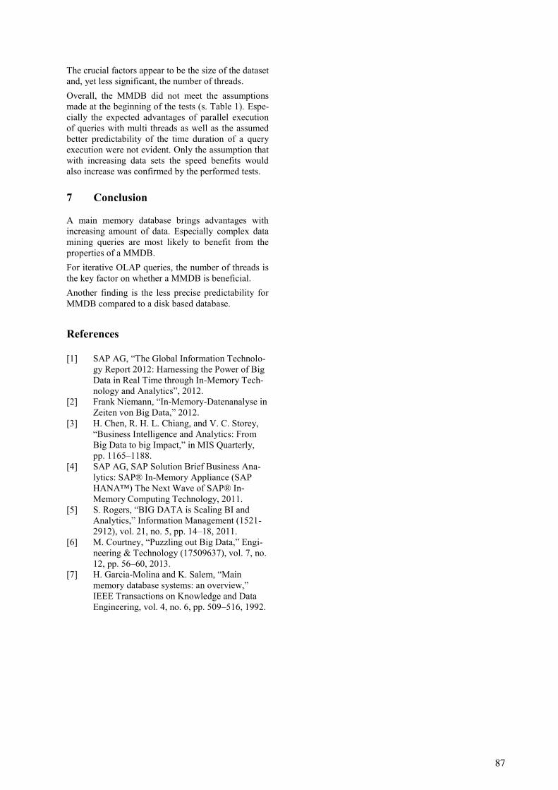
The crucial factors appear to be the size of the dataset

and, yet less significant, the number of threads.

Overall, the MMDB did not meet the assumptions

made at the beginning of the tests (s. Table 1). Espe-

cially the expected advantages of parallel execution

of queries with multi threads as well as the assumed

better predictability of the time duration of a query

execution were not evident. Only the assumption that

with increasing data sets the speed benefits would

also increase was confirmed by the performed tests.

7 Conclusion

A main memory database brings advantages with

increasing amount of data. Especially complex data

mining queries are most likely to benefit from the

properties of a MMDB.

For iterative OLAP queries, the number of threads is

the key factor on whether a MMDB is beneficial.

Another finding is the less precise predictability for

MMDB compared to a disk based database.

References

[1] SAP AG, “The Global Information Technolo-

gy Report 2012: Harnessing the Power of Big

Data in Real Time through In-Memory Tech-

nology and Analytics”, 2012.

[2] Frank Niemann, “In-Memory-Datenanalyse in

Zeiten von Big Data,” 2012.

[3] H. Chen, R. H. L. Chiang, and V. C. Storey,

“Business Intelligence and Analytics: From

Big Data to big Impact,” in MIS Quarterly,

pp. 1165–1188.

[4] SAP AG, SAP Solution Brief Business Ana-

lytics: SAP® In-Memory Appliance (SAP

HANA™) The Next Wave of SAP® In-

Memory Computing Technology, 2011.

[5] S. Rogers, “BIG DATA is Scaling BI and

Analytics,” Information Management (1521-

2912), vol. 21, no. 5, pp. 14–18, 2011.

[6] M. Courtney, “Puzzling out Big Data,” Engi-

neering & Technology (17509637), vol. 7, no.

12, pp. 56–60, 2013.

[7] H. Garcia-Molina and K. Salem, “Main

memory database systems: an overview,”

IEEE Transactions on Knowledge and Data

Engineering, vol. 4, no. 6, pp. 509–516, 1992.

87

Full Text processing using SAP HANA

(Author)

Jevgenij Jakunschin

University of Wismar

[email protected]

(Supervisor)

Prof. Dr.-Ing. Antje Düsterhöft

University of Wismar

[email protected]

Abstract

This project seeks to create an evaluation of full text

search and related features of the SAP HANA data-

base and other No-SQL and in-memory databases.

1 Introduction

In today’s environment of rapidly evolving technolo-

gies and database systems, with the boom of NO-

SQL databases and the rising problem of the “big

data” issue, new projects are rapidly created, merged,

changed and even aborted.

Most new systems are very bare bone, offering little

possibilities and description of their capabilities for

specific tasks, e.g. full text search processing.

This project, as part of a master thesis, seeks to test

different systems, primary SAP HANA, on their

possibilities, performance, stability, scalability and

precision in big data full text tasks. It also aims to

compare the algorithmic base and provide a graphical

representation of the results.

During the course of this project, it will be also ex-

tended with information on the performance of dif-

ferent modern NO-SQL and in-memory databases in

order to provide an in-depth comparison of different

systems, their performance and features.

2 Project state

A large amount of full text data is required in order to

pursue the goals of the project.

A big database of books and articles (initially in *.txt

format) with irregular file sizes has been prepared in

order to perform such tests.

The books have been collected, using the Project

Gutenberg ( http://www.gutenberg.org/ ) database.

Only books in .txt format and (mostly) mostly Eng-

lish books have been selected for the tests. Overall a

database of 11.531 files, with a total size of 4.34

gigabytes has been collected and prepared for the

tests.

Figure 1: twitter crawler

Afterwards these files have been run through a spe-

cial application to remove special signs, HTML en-

coding, restrict line length and fix some other format-

ting problems that might be encountered during the

tests. The program also merges files into Microsoft

Excel Comma Separated Values (CSV) format to

prepare them for the FTP upload into the database.

The application also provides the possibility to split

and merge files, in order to test the optimal table

length and storage strategy.

The database already provides sufficient material in

order to make performance tests.

However, the project also contains a small applica-

tion to quickly gather full text data from gather from

a small twitter crawler for special tests, like fuzzy

search efficiency, performance and precision. Initial-

ly the data from both applications is (initially) stored

in a 3-column CSV file, consisting out of an ID-key

value, a line-value for splitting long texts and the text

field.

Additional fields for evaluations and tests are added

from the SAP HANA studio during the progress.

89

Figure 2: Gutenberg->Csv Converter

In addition, a “troublemaker” application has been

designed to create, recorded edits in different files in

order to test the fuzzy search possibilities and preci-

sion of a database.

Figure 3: "Troublemaker" application

2.1 Running tests

The text data from the resources above is uploaded to

the SAP HANA database using the SFTP protocol

and is then imported from the SAP HANA Studio.

The text fields are indexed with the “text” (or “short

text”) type and the tables are being prepared for the

following tests:

The results are going to be evaluated statistically

upon the following criteria:

- Supported features

- Indexing options and their performance, fea-

tures and limits (short text and text)

- Performance (full text search, insert state-

ments, fuzzy search upload etc.,)

- Stability and accessibility

- Scalability (depending on cell size, table

size, document size and search complexity)

- Comparison to SQL-Standards

- Other statistics

In addition the following full text specific criteria are

being tested:

- Fuzzy Search possibilities

- Fuzzy Search precision, false positives, false

negatives, optimal factor

- Syntax analysis options

- Language options

- Indexing options

- Full text search limits

Over the course of the project, different databases

will undergo the same processes to create a statistics

database.

Currently the project is done with the phase of data

collecting, converting and manipulating and the first

tests and test data with SAP HANA are being pre-

pared and uploaded.

The database will be tested on the features described

above, by performing different queries and measur-

ing and comparing the results.

Part of the tests also includes searches with different

databases sizes and interpolating and approximating

the response times in order to predict the scalability

of the project with full-text searches with an auto-

mated indexing.

A graphical interface is designed in order to quickly

automate and represent different findings for a data-

base in chart form and compare its performance

against other databases with similar setup.

The charts will also represent the performance, preci-

sion and scalability relation in comparison to differ-

ent table sizes, text indexes and text lengths.

2.2 Next Steps

As the SAP HANA part of the project is pretty

young, a multitude of steps is still to come.

Other databases are going to be tested in a similar

manner, as described previously.

The project also seeks to test databases with different

text languages in order to evaluate the syntax analysis

options.

The troublemaker application will be used in order to

test the capabilities of different databases setups to

work with flawed data, using algorithms like fuzzy

search.

Finally a big part of the project is to test different full

text storage and indexing strategies in order to mini-

mize the performance loss, coming from non-optimal

storage and scheme approaches.

2.3 Conclusions

The project is in the state of gathering it’s most vital

data right now and will be ready to present it’s find-

ings soon.

Since the project is in the critical phase, where it is

ready to perform the required tests and draw conclu-

sions, I would also like to ask for an extension.

90

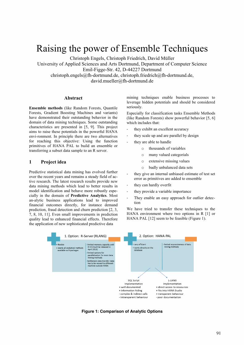
Raising the power of Ensemble TechniquesChristoph Engels, Christoph Friedrich, David Müller

University of Applied Sciences and Arts Dortmund, Department of Computer Science

Emil-Figge-Str. 42, D-44227 Dortmund

[email protected], [email protected],

[email protected]

Abstract

Ensemble methods (like Random Forests, Quantile

Forests, Gradient Boosting Machines and variants)

have demonstrated their outstanding behavior in the

domain of data mining techniques. Some outstanding

characteristics are presented in [5, 9]. This project

aims to raise these potentials in the powerful HANA

envi-ronment. In principle there are two alternatives

for reaching this objective: Using the function

primitives of HANA PAL to build an ensemble or

transferring a subset data sample to an R server.

1 Project idea

Predictive statistical data mining has evolved further

over the recent years and remains a steady field of ac-

tive research. The latest research results provide new

data mining methods which lead to better results in

model identification and behave more robustly espe-

cially in the domain of Predictive Analytics. Most

an-alytic business applications lead to improved

financial outcomes directly, for instance demand

prediction, fraud detection and churn prediction [2, 3, 7, 8, 10, 11]. Even small improvements in prediction

quality lead to enhanced financial effects. Therefore

the application of new sophisticated predictive data

mining techniques enable business processes to

leverage hidden potentials and should be considered

seriously.

Especially for classification tasks Ensemble Methods

(like Random Forests) show powerful behavior [5, 6]

which includes that:

- they exhibt an excellent accuracy

- they scale up and are parallel by design

- they are able to handle

o thousands of variables

o many valued categorials

o extensive missing values

o badly unbalanced data sets

- they give an internal unbiased estimate of test set

error as primitives are added to ensemble

- they can hardly overfit

- they provide a variable importance

- They enable an easy approach for outlier detec-

tion

We have tried to transfer these techniques to the

HANA environment where two options in R [1] or

HANA PAL [12] seem to be feasible (Figure 1).

Figure 1: Comparison of Analytic Options

91

Because the second option makes use of the compu-

ting power of the HANA hardware and minimizes data

transfer from the database to the analytic function we

are in favor of option 2. (following the paradigm:

“bring the analytic function to the data”!). The project

will try to implement option 2 and option 1 (which

seems to be straightforward) and will compare both re-

sults by application to example classification prob-

lems.


The project has needed a HANA environment (HW

and SW) with the latest PAL distribution available and

an R installation optionally.

An exclusive access was necessary for performance

measurements at the end of the project for approx. five

nights.

3 Findings

3.1 Analysis of standalone weak learners

The basis of ensembles are weak learners in form of

decision trees in our case. On the PAL side we use the

C4.5 decision tree algorithm from the library with var-

iations of learning parameters while on the R side we

apply the C5.0 implementation with default settings.

The PAL C4.5 shows some restrictions in terms of

flexibility w.r.t. an ensemble usage: Pruning is man-

datory and randomization on node level is not possible

yet. It turns out (see Annex) that the PAL C4.5 imple-

mentation compared to a similar R approach shows

significant longer training times by a magnitude. The

reason is given by the fact that this implementation is

relatively new and programmers have not taken the

full potential of the HANA architecture [4]. The accu-

racies of both approaches on different datasets are sim-

ilar with some variations of the results due to training

parameter variations.

3.2 Analysis of ensembles

Ensembles are created by using weak learners and the

principles of randomization, boosting and bagging. In

our case we have to apply some simplifications due to

the limited flexibility of the PAL C4.5 decision tree

implementation: Randomization can be done on a tree

level instead of a node level only and pruning of trees

has to be accepted which is omitted in standard ensem-

ble methods. Additionally sampling with replacement

is hard to implement and is done without replacement

here instead. Two datasets are used (OPTICAL_REC

and KRKOPT). While the results in OPTICAL_REC

are comparable in accuracy, there is a large deviation

in the KRKOPT dataset with poor performance in the

case of two attributes per tree in accordance with de-

fault setting (#attributes per split = sqrt(#attributes)),

see Annex. It seems that these default settings on the

node level cannot be transferred on tree level for da-

tasets in general. If we increase the number of attrib-

utes per tree the results are improving. It is remarkable

that the PAL ensemble method (RF) in the

OPTICAL_REC dataset shows significantly superior

accuracy than the PAL decision tree (DT).

4 Next steps

In the recent research and project period we have in-

vestigated the behavior of both options followed by a

comparison. It could be shown that there are some

open issues concerning the one to one mapping of the

R-server approach to HANA-PAL:

- Performance issues

- Mandatory Pruning of Decision Trees

- Missing Randomization of Input Attributes

- Sampling with Replacement

Due to these unexpected observations during the pro-

ject the extension of ensembles by using Stochastic

Gradient Boosting [16] could not be achieved within

the first project period. Furthermore it turns out that

the provision of ensembles will need dedicated

SQLScript programming skills which makes the appli-

cation of PAL methods for “normal” users difficult.

Additionally we have experienced limited expressive-

ness of the SQLScript wrapper call technique.

5 Extension

The main objective of this project is to address the re-

maining methodic work regarding ensemble methods

by implementing Stochastic Gradient Boosting and to

simplify the allocation of ensemble methods by

providing a graphical user interface.

In order to deal with the situation from the last spring

period we propose the following activities:

5.1 Activity “Migration”

Migration of ensemble technique to native L-LANG.

At the moment L-LANG shows some restrictions like

limited reusability and no direct support for parallel-

ism. This restrictions will be resolved probably within

next weeks and month, so this project is able to make

use of these improvements.

5.2 Activity “HANA Studio Embedding”

Embedding the ensemble functionality in the HANA

Studio Workflow Tool as L-LANG node due to the

agreement with [4].

5.3 Activity “Stochastic Gradient Boosting”

Add the Stochastic Gradient Boosting method [13]

into the ensemble creation. Because the weak learners

within the ensemble will be learned sequentially, the

algorithm is able to use the information gained during

92

the training of the initial learners for an improved data

selection for the remaining learners.

5.4 Conclusions

The implementation of HANA PAL functionality still

undergoes a steady extension. As a consequence the

comparability of different approaches and options in

implementing Ensemble Techniques remains difficult.

Nevertheless we expect a richer and more complete set

of functions especially in the PAL context in the near

future such that remaining differences between PAL

and R will vanish over time.

References

[1] J. Aswani; J. Doerpmund: "Advanced Analytics with

R and SAP HANA", Slideshare. Retrieved 2012-03-

14 (2012).

[2] R. E. Banfield; R.E., el. al.: “A Comparison of Deci-

sion Tree Ensemble Creation Techniques”, IEEE

Transactions on Pattern Analysis and Machine Intelli-

gence, Vol. 29, No. 1 (2007).

[3] S. Benkner, A. Arbona, G. Berti, A. Chiarini, R. Dun-

lop, G. Engelbrecht, A. F. Frangi, C. M. Friedrich, S.

Hanser, P. Hasselmeyer, R. D. Hose, J. Iavindrasana,

M. Köhler, L. Lo Iacono, G. Lonsdale, R. Meyer, B.

Moore, H. Rajasekaran, P. E. Summers, A. Wöhrer

und S. Wood: „@neurIST Infrastructure for Advanced

Disease Management through Integration of Heteroge-

neous Data, Computing, and Complex Processing Ser-

vices“, DOI:10.1109/TITB.2010.2049268, IEEE

Transactions on Information Technology in BioMedi-

cine, 14(6), Seite 1365 - 1377, (2010).

[4] J.-H. Böse, SAP Innovation Center Potsdam, personal

communication, Aug. 2013.

[5] L. Breiman: „RF / tools – A Class of Two-eyed Algo-

rithms“, SIAM Workshop http://www.stat.berke-

ley.edu/~breiman/siamtalk2003.pdf , (2003).

[6] L. Breiman: “Random Forests”,

http://www.stat.berkeley.edu/~breiman/

random-forests-rev.pdf, (1999).

[7] C. Engels; W. Konen: „Adaptive Hierarchical Fore-

casting”. Proceedings of the IEEE-IDACCS 2007

Conference, Dortmund (2007).

[8] C. Engels: „Basiswissen Business Intelligence.“, W3L

Verlag, Witten (2009).

[9] J. Friedman: „Computational Statistics & Data Analy-

sis”, Volume 38, Issue 4, 28 February 2002, Pages

367–378, http://dx.doi.org/10.1016/S0167- 9473(01)00065-2, (2002).

[10] M. Hülsmann; D. Borscheid, C. M. Friedrich und D.

Reith: "General Sales Forecast Models for Automo-

bile Markets and their Analysis", Transactions on Ma-

chine Learning and Data Mining, Volume 5, Number

2, Seite 65-86, 2012.

[11] G. Üstünkar; S. Özögür-Akyüz; G. W. Weber; C. M.

Friedrich und Y. A. Son, „Selection of Representative

SNP Sets for Genome-Wide Association Studies: A

Metaheuristic Approach“, DOI:10.1007/s11590-011-

0419-7, Optimization Letters, Volume 6(6), Seite

1207-1218, (2012).

[12] PAL, https://help.sap.com/hana/hana_dev_pal_en.pdf

(2013).

[13] G. Ridgeway: „Generalized Boosted Models: A guide

to the gbm package”. http://cran.r-pro-

ject.org/web/packages/gbm/vignettes/gbm.pdf, (2007).

93

Annex: Detailed results

The following tables summarize the results of our experiments with decision trees and ensembles over decision

trees in terms of performance and crossvalidated accuracy (DT means Decision Tree, RF abbreviates the

ensemble method Random Forest. Datasets can be found at http://archive.ics.uci.edu/ml/datasets.html.

Dataset DT / RF PAL / R rows

used

Inputrows

Training

Parameter Training Performance

(overall)

for RF on PAL

Performance

(Training)

(R C5.0 / PAL

C4.5)

SIZE DT

R C4.5 / PAL

C4.5)

Inputrows

Testing

Parameter

Testing

Performance

(Testing)

(R C50 / PAL

C45)

Accuracy

(R C50 CROSS /

PAL C45 CROSS)

Dataset IRIS

(150rows)

DT PAL 150 (all) 94 THREAD = 16

SPLIT MODEL = 1

PMML EXPORT = 2

MIN_REC = 2

-- 95 ms 12 56 THREAD = 16 34 ms Accuracy = 0,94

++ = 0,98

-- = 0,91

R 150 (all) 94 -- -- 13 ms 7 56 -- 6ms Accuracy = 0,92

++ = 0,98

-- = 0,86

Dataset KRKOPT

(28056rows)

DT PAL 28.056

(all)

1.7675 THREAD = 16

SPLIT MODEL = 1

PMML EXPORT = 2

MIN_REC = 2

-- 7,08 sec 23.237 10.381 THREAD = 16 2,23 sec Accuracy = 0.585

++ = 0.595

-- = 0.576

R 28.056

(all)

1.7675 -- -- 1.13 sec 6.017 10.381 -- 332 ms Accuracy = 0,63

++ = 0,635

-- = 0,621

RF PAL 28.056

(all)

Pool 1.7675

random

THREAD = 16

SPLIT MODEL = 1

PMML EXPORT = 2

MIN_REC = 2

tree = 100

Attribute per Tree = 2

18 min -- - 10.381 THREAD = 16 -- Accuracy = 0,272

R 28.056

(all)

Pool 1.7675

random

tree = 100 -- 14,17 sec -- 10.381 -- 231 ms Accuracy = 0,68

94

Integration of a VEE-Framework within a Smart Gateway into SAPHANA

Jan-Patrick WeißUniversity of Oldenburg

Department of Computer ScienceUhlhornsweg 84

D-26129 [email protected]

Benjamin ReineckeUniversity of Oldenburg



Marco LuchtUniversity of Oldenburg



Jad AsswadUniversity of Oldenburg



Jan Hendrik WegeUniversity of Oldenburg



Christoph WaltherUniversity of Oldenburg



Abstract

The energy market is changing by legislation so by2020 smart meters will be installed in most house-holds. Therefore the IT systems of energy companieshave to adjust to deal with the growing amount of mea-sured data. With smart meters it is possible to mea-sure the consumption every 3 minutes and shorter in-stead of measuring only one annual value. This nearreal time data consumption allows companies to cre-ate new business use cases. They can for example pre-dict the usage of their grids and close short time con-tracts with suppliers to meet the demands. Further-more there are new possibilities for analysis and as-surance of data quality. In order to assure a definedintegrity, possible missing or false values of the avail-able measuring data have to be corrected. The projectdeals with these problems of data quality and han-dling of these massive data. To ensure integrity andthe best quality of data, a VEE-Framework (Valida-tion, Estimation, Editing) will take a place. The VEE-Framework shall be implemented within a Smart Gate-way and integrated into SAP HANA to benefit from the

efficiency of in-memory-database technology.

1 Introduction

This document shows the main idea of the project ”In-tegration of a VEE-Framework within a Smart Gate-way into SAP HANA”. At first the business contextof smart metering in modern households is described.After that an explanation of the VEE-Framework willdemonstrate how smart meter data can be used andhow data is being precessed. In the part ”objectivetarget” the goals of the project are described. Further-more the reasons to use SAP HANA for this project areexplained. At the end new insights and further stepsand outlook are shown.

2 Smart Metering

Smart Metering describes a method to count, docu-ment and analyze the consumption (electricity, gas,water etc.) by using electrical meters. The measure-ment data can be recorded in individual time inter-

95

vals (minutes, hours, days etc.) and is automaticallysubmitted to the measurement data responsible, whichwill submitted to the supplier, which can use this infor-mation e.g. for monitoring or billing processes. Smartmeters enable two-way communication between themeter and the suppliers’ system. Furthermore they canbe used to gather information for remote reporting.When using additional technical functions, the con-sumer is able to monitor his consumption and to makeconstant analyzes. Energy hogs can be identified andthe use of energy-intensive devices can be switched totime frames, where energy is less expensive. That maylead to decrease energy costs. Furthermore smart me-ters can be part of a smart grid.

3 VEE-Framework - Validation, Estima-tion, Editing

Metering data from different sources is a very exten-sive process which needs to provide a large amount of functionality and robustness, not only hardware but software based. However, potential errors can never be barred and have to be treated respectively. Therefore a process, called Validation, Estimation and Editing (VEE) is introduced. The main objective is to offer a set of methods which allow a partly automated ap-proach of specific error handling based on predefines rules. This allows business users to identify erroneous and potentially problematic data before it is used by downstream applications. It is important to state that all changes that are made to the considered data have to be logged in order to reconstruct them in the future.

In a first step, the source dataset needs to be validatedin order to determine inconsistencies, e.g. missingvalues, duplicates or spikes. Therefore the necessarymeter data has to be identified, collected and version-ized. Afterwards, several tests like Time Tollerance-,Sum- and Spike Checks are peformed and evaluatedon the specific values. The various test types areidentified and selected automatically via configurableparameters within the meter read. Depending on thetest results, the individual values need to be marked asfailed and subsequently further processed.

During estimation phase, all previously marked valuesshall be adapted and corrected in order to correspondto their specific requirements. Therefore severalappropriate replacement values are generated bychoosing a specific set of customer based methodsand applying them to the read meter data. These rulescan be assigned to individual customers as well asto groups of various customers and are furthermoreexchangeable in any order. It is important that thosevalues which have been estimated or treated in anyway are marked accordingly in order to identify themfor later use.

The third step of VEE process implies the actual edit-ing of the available meter data. This includes writingthe individual replacement value into the data set aswell as setting the status parameter to its designatedvalue (see figure 1).

Figure 1: VEE process

Due to the customizable sets of rules, the automaticdata validation and estimation and the consecutivelogging functionalities, the VEE process guaranteesan accurate and quick verification of read meter datawhich is a necessary assumption for various businessuse cases.

4 Objective Target

The project group is aiming to develop an SAP-HANA appliance which fits into the existing systemsused for measuring customers’ energy consumptionand creating the customers’ invoices. Therefore thefollowing steps shall be taken:

96

1. When meter-values for a certain customer are re-quested by SAP e.g. for creating an invoice, SAPHANA loads the data (from the PI-Server or theCX4U Smart-Gateway).

2. The loaded consumption values from the gas me-ters are checked for faulty or even missing val-ues (either within the Smart Gateway or in SAPHANA).

3. If such a value is found, it is being replaced bya calculated value which was calculated by a cer-tain pattern fitted to the customer.

4. The generated value is logged to a file, so that theinvoice stays transparent.

5. Both, calculated and measured values are takento SAP so that the invoice can be created.

As the calculation method for faulty and missing val-ues depends on the customer and can be changed, thecalculation in SAP HANA is just temporary and thevalues are only passed to the system which requestedthem and will be deleted afterwards.

5 Reasons to use SAP HANA for thisproject

SAP HANA is used to optain high performance in pro-cessing large amounts of heterogeneous data. By con-necting households to smart meters, the massive data volumes increase, since there is not as yet, an annual settlement, but a possibility to measure every 15 min-utes, or at even shorter intervals, energy consumption data. Every Smart Meter generates 768 bytes of data per day - with a base of 15,000 meters in the used demonstration system, we are talking about approxi-mately 330 gigabytes of data in an accounting period (normally a month) [1].In order to forecast electricity consumption for a day, we have to process nearly 11 gigabytes of data. With the available data; analysis, forecasting and quality of results can be increased. In order to generate settle-ments it is necessary to have correct and complete val-ues. SAP HANA supports this process with statistical functions to find and eliminate missing and non-valid data. This functionality is also called VEE (Valida-tion, Estimation, Editing). When using SAP HANA for processes such as analysis or prediction calcula-tions, it is necessary to integrate the functionalities of SAP HANA with the VEE-Framework within the Smart Gateway.

6 New Insights

Implementing the VEE Framework within SAPHANA and connecting SAP HANA with SmartGateway leads us to new insights through benefiting

from real time processing of the in-memory com-puting technology. SAP HANA with its simplicityand easy to handle interfaces and functions presentsa full database platform in addition to its analyticaland transactional capabilities within the attribute, theanalytic and the calculation views and other artifacts.

However, despite the capability of HANA to intercon-nect with other SAP or non-SAP systems or databases,there is always latency in loading and exporting themetering data into and from SAP HANA. These twooperations are not automated and time consuming,which is very crucial to our process. In order to handlethe data transfer the project group has to provide a so-lution that transfers the metering data fast, efficientlyand accurately.

7 Further Steps and Outlook

Currently the project group cooperates with CX4UConsulting and analyses the data which is provided bythe product SmartGateway. It is important to under-stand how the interfaces of the SmartGateway workto get the necessary data into SAP HANA. The nextsteps are to show - within a proof of concept - inwhich way the VEE-Framework can be implementedinto SAP HANA, and in which way SAP HANA canbe connected or intgrated with Smart Gateway. Thereshould be several alternatives and the best one shouldbe shown in a prototype.

References

[1] C. Kuhlmann. E-Mail, 06.08.2013. CX4U AG, Olden-burg.

97

Next Generation Operational Business Intelligence exploring the example of the bake-off process

Alexander Gossmann Research Group Information Systems University of Mannheim

[email protected]

Abstract

Large retail organizations have to plan customer demands accurately, to achieve customer satisfaction and loyalty. The primary objective is to avoid out-of-shelf situations. On the other hand, losses of perished goods, especially in case of fresh food, have to be minimized. The handling of the trade-off between availability and loss can be dramatically improved by a real-time analytic system. The challenge is to analyze large amounts of data (big data), typically derived from the transactions in the retail process, enhanced by external data, like weather and holi-days. Different management groups require specific information with short response times at reasonable costs. Transferred to the retail domain, local store managers are focused on operational decision mak-ing, while top management requires a view on the business at a glance. Both requirements rely on transactional data, where-as the analytic views on this data differ completely. Thus different data mining capabilities in the under-lying software system are targeted, especially related to processing masses of transactional data. The examined software system is a SAP HANA in-memory appliance, which satisfies the aforemen-tioned divergent analytic capabilities, as will be shown in this work.

Introduction (Project Idea)

Operational Business Intelligence is becoming an increasingly important in the field of Business Intel-ligence, which traditionally was targeting primarily strategic and tactical decision making [1]. The main idea of this project is to show that reporting require-ments of all organizational levels (operational and strategic) can be fulfilled by an agile, highly effective data layer, by processing directly operative data. The reason for such architecture is a dramatically de-creased complexity in the domain of data warehous-ing, caused by the traditional ETL process [2]. This requires a powerful and flexible abstraction level of the data layer itself, as well as the appropriate pro-cessability of huge amounts of transactional data. The SAP HANA appliance software is currently released in SPS 05. Important peripheral technologies have been integrated, such as the SAP UI5 Presenta-tion Layer and the SAP Extended Application Ser-

vices, a lightweight Application Layer. This project proves the tremendous possibilities offered by this architecture which allows a user centric development focus. This report is organized in the following chapters. The first chapter provides a general overview of the explored use case. In the second chapter the used resources will be explained. The third and fourth chapters contain the current project status and the findings. This Document concludes with an outlook on the future work in the field.

1 Use Case

This project is observing a use case in the field of fast moving goods of a large discount food retail organi-zation. Specifically, the so called bake-off environ-ment is taken into account. Bake-off units reside in each store and are charged with pre-baked pastries based on the expected demand. The trade-off be-tween product availability and loss hereby is ex-tremely high. From the management point of view, the following user group driven requirements exist: On the one hand, placing orders in the day to day business re-quires accurate and automated data processing, to increase the quality of the demand forecast. On the other hand, strategic decision makers need a flexible way to drill through the data on different aggregation levels, to achieve a fast reaction time to changing market conditions. The observation period of two years is considered. The basic population consists of fine grained, minute wise data for thousands of bake-off units, providing all facts related to the bakery process.

1.1 Store Level Requirements On the store level, the store manager will be support-ed with matters regarding daily operational demands. Primarily for order recommendations, a certain amount of historical data is taken into account to satisfy the appropriate statistical calculation on time series. Additionally location related and environmen-tal information increases the accuracy of the forecast-ing model. Environmental variables, like historical weather and holidays, are considered in correlation with historical process data to improve the forecast model. Furthermore, forecasted weather data and upcoming holidays are taken into account for ex-ante

99

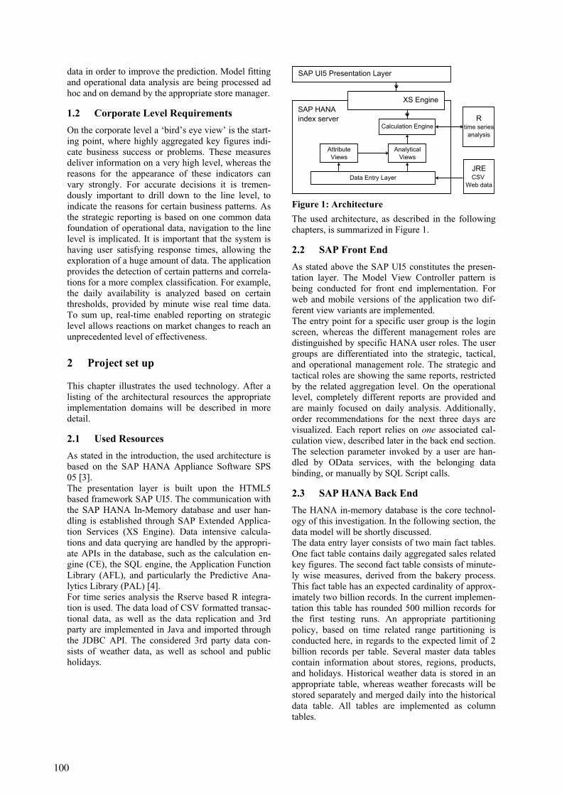
data in order to improve the prediction. Model fitting and operational data analysis are being processed ad hoc and on demand by the appropriate store manager.

1.2 Corporate Level Requirements On the corporate level a ‘bird’s eye view’ is the start-ing point, where highly aggregated key figures indi-cate business success or problems. These measures deliver information on a very high level, whereas the reasons for the appearance of these indicators can vary strongly. For accurate decisions it is tremen-dously important to drill down to the line level, to indicate the reasons for certain business patterns. As the strategic reporting is based on one common data foundation of operational data, navigation to the line level is implicated. It is important that the system is having user satisfying response times, allowing the exploration of a huge amount of data. The application provides the detection of certain patterns and correla-tions for a more complex classification. For example, the daily availability is analyzed based on certain thresholds, provided by minute wise real time data. To sum up, real-time enabled reporting on strategic level allows reactions on market changes to reach an unprecedented level of effectiveness.

2 Project set up

This chapter illustrates the used technology. After a listing of the architectural resources the appropriate implementation domains will be described in more detail.

2.1 Used Resources As stated in the introduction, the used architecture is based on the SAP HANA Appliance Software SPS 05 [3]. The presentation layer is built upon the HTML5 based framework SAP UI5. The communication with the SAP HANA In-Memory database and user han-dling is established through SAP Extended Applica-tion Services (XS Engine). Data intensive calcula-tions and data querying are handled by the appropri-ate APIs in the database, such as the calculation en-gine (CE), the SQL engine, the Application Function Library (AFL), and particularly the Predictive Ana-lytics Library (PAL) [4]. For time series analysis the Rserve based R integra-tion is used. The data load of CSV formatted transac-tional data, as well as the data replication and 3rd party are implemented in Java and imported through the JDBC API. The considered 3rd party data con-sists of weather data, as well as school and public holidays.

Figure 1: Architecture The used architecture, as described in the following chapters, is summarized in Figure 1.

2.2 SAP Front End As stated above the SAP UI5 constitutes the presen-tation layer. The Model View Controller pattern is being conducted for front end implementation. For web and mobile versions of the application two dif-ferent view variants are implemented. The entry point for a specific user group is the login screen, whereas the different management roles are distinguished by specific HANA user roles. The user groups are differentiated into the strategic, tactical, and operational management role. The strategic and tactical roles are showing the same reports, restricted by the related aggregation level. On the operational level, completely different reports are provided and are mainly focused on daily analysis. Additionally, order recommendations for the next three days are visualized. Each report relies on one associated cal-culation view, described later in the back end section. The selection parameter invoked by a user are han-dled by OData services, with the belonging data binding, or manually by SQL Script calls.

2.3 SAP HANA Back End The HANA in-memory database is the core technol-ogy of this investigation. In the following section, the data model will be shortly discussed. The data entry layer consists of two main fact tables. One fact table contains daily aggregated sales related key figures. The second fact table consists of minute-ly wise measures, derived from the bakery process. This fact table has an expected cardinality of approx-imately two billion records. In the current implemen-tation this table has rounded 500 million records for the first testing runs. An appropriate partitioning policy, based on time related range partitioning is conducted here, in regards to the expected limit of 2 billion records per table. Several master data tables contain information about stores, regions, products, and holidays. Historical weather data is stored in an appropriate table, whereas weather forecasts will be stored separately and merged daily into the historical data table. All tables are implemented as column tables.

SAP HANAindex server

SAP UI5 Presentation Layer

XS Engine

Rtime series

analysis

AnalyticalViews

AttributeViews

Data Entry Layer

Calculation Engine

JRECSV

Web data

100

Upon this data entry layer several attribute views are implemented, building up the product, store and regional dimensions. The time dimension is based on the generated time table with minutely level of granu-larity (M_TIME_DIMENSION), provided by HANA standardly. The two analytical views contain the fact tables, whereas the daily based fact table is additionally enhanced by the weather and holiday dimensions. Based on this multidimensional data model eight calculation views are implemented, to satisfy user reporting scenarios about availability, loss, and sales on tactical and strategic level. Additionally one cal-culation view provides reporting needs on operational level, showing the relevant process information of the current and previous days. For more sophisticated data mining on the strategic level, as well as data preprocessing of time series data, PAL is used [5]. Specifically the linear regres-sion model function is used to draw trends of dynam-ically aggregated sales data over time. Further the anomaly detection function is used for outlier detec-tion in daily sales data.

2.4 Peripheral technology The load of historic and transactional data is handled by a proprietary Java import module, using the JDBC API. The reason for this implementation mainly relies on huge amount of heterogeneous CSV format-ted files. Approximately two hundred thousand dif-ferent types of CSV files have been imported into the HANA database. Therefore, a special bulk load strat-egy has been used, especially in spite of the insert properties of column oriented tables in the entry layer. Furthermore, historic weather data as well as weather forecast and holiday data is loaded via the JDBC interface of the import module. Holidays Both school and public holidays have been down-loaded for the past two years, and until the year 2015 from the online portal 'Schulferien.org'. The data is available in the iCal format, and covers all dates for the different states of Germany. These files were loaded into the HANA index server, after conversion into CSV format, using the appropriate build in wiz-ard. Weather The historical weather data has been imported from the web weather API ‘wonderground.com’. For mod-el training of the forecast module, the corresponding time interval values of daily, city wise consolidated store data was called from the API. This results in approximately one million JSON files (one file corre-sponds to one data record), generated by the REST interface, afterwards converted into CSV format and loaded via JDBC of the import module.

Forecast The demand forecast requirements are primarily developed using the R environment. The appropriate time series are generated on demand, and invoked by a store manager who is responsible for one’s store. As stated in the previous section, the time series are being preprocessed in advance by the PAL frame-work primarily for performance reasons. The important outlier detection and handling have been additionally implemented in the R environment, as here more advanced algorithms are available in the R community. Furthermore, two different forecast models have been utilized for comparison reasons. The ARIMA (Auto Regressive Integrated Moving Average) model as well as the ANN (Artificial Neu-ronal Network) based model have been observed.

2.5 Development environment The eclipse based HANA Studio is used as the main IDE for the development. In addition to the newly introduced SPS05 features, regarding the ‘HANA development’ perspective, the Java import module is implemented as well. For usability reasons the following implementation strategy of the R environment has been utilized: Each developer uses a local R runtime for coding R script and model testing. The appropriate time series data is supplied through the ODBC interface. After finaliz-ing a model in R, it is transformed into the HANA environment using the RLANG extension in SQL Script [5]. All artifacts, including java classes, java script, UI5 artifacts and R script have been set under version control with git [6]. The prototype has been completely redesigned re-garding the SAP HANA components. The SAP HANA repository has been used for this purpose, to store all relevant design time artifacts like:

- hdb tables - hdb roles - procedures

3 Findings

This chapter contains findings on technological as well as on the process level. The findings will be explained analogous to the outline of the previous chapter. In conclusion the outcome of this project will be summarized.

3.1 SAP Front End Through the tight integration of the controller and model layer, the presentation layer profits of the advantage of a high abstraction level. The data bind-ing feature of the OData services is especially benefi-cial for strategic and tactical reporting. Hereby flexi-ble data navigation for the top management user is provided, by selecting free time intervals and break-

101

ing down into different products, regions, or stores. Never the less, the store management invokes an ad hoc data mining and forecasting capability by calling a SQL Script procedure through a Java Script DB connection call. For parameterization of the calculation views the following limitations exist:

exclusively input parameters are used, in-stead of variables for performance reasons

for input parameters, no ranges are support-ed and graphical calculation views requireadditional filter expressions

character based date parameters work withthe OData interface (thus no type safety isprovided, implicit cast)

3.2 SAP HANA Back End In the previous chapter (2.3) the data model has been explained. The biggest column based table contains two years of minutely based transactional data. It has been partitioned by regions. The response times of the appropriate calculation view calls are absolutely satisfying . Nevertheless, the following main re-strictions have been experienced which are listed by the appropriate domain: Predictive Analytics Library

usability of PAL functions is inconvenientand non-transparent

restrictive parameterization policy very limited exception handling

The restriction in the design time usability especially in the case of PAL, compromises the performance experience of the data analysis. The AFL framework is in a relatively early stage of maturity and in this project context, only few func-tions could be utilized. The major functionality in the area of time series analysis has been conducted in the R environment, as stated in the next section.

3.3 Forecast The demand forecast for each store is calculated on demand. The appropriate time series is generated and sent, together with the belonging weather and holiday information to the R runtime. Hence the sent data frame to R contains daily related time series derivates of additional environmental data to the historic sales data for a certain pastry and store. Time Series Preprocessing (Outlier Adjustment) For comparison reasons the outlier detection is being performed with PAL and in a second scenario in R. In case of PAL preprocessing, the outliers are marked in the time series data frame provided to R. The used PAL function is PAL_ANOMALY_DETECTION with the following parameterization:

Parameter Value Comment

THREAD_NUMBER 4

GROUP_NUMBER 3 number of clusters k

OUTLIER_DEFINE 1 max distance to cluster center

INIT_TYPE 2

DISTANCE_LEVEL 2

MAX_ITERATION 100

Table 1: PAL parameterization As depicted in Table 1, the used PAL function uses a k-means cluster algorithm, whereas GROUP-_NUMBER corresponds to the number of associated clusters (k). Please note that this function detects always one tenth of the underlying number of lags in each time series as outliers. This could not be con-trolled by the parameter OUTLIER_PERCENTAGE, as expected and thus, limits this function enormously. In the R environment the k-means clustering for outlier detection is used as well. A straightforward approach of outlier handling is used. The majority of given outliers belongs to the class of additive outliers due to public holiday related store closing. The effect is even more significant, the longer a closing period is. Here the precedent open business date shows an abnormal high characteristic. Other outlier classes are by far less significant and cannot be assigned directly to events. Different outlier handling strategies have been tested and implemented, and will be investigat-ed in further proceedings. ARIMA based forecast An automated ARIMA model has been implemented in R. The used package is mainly the package 'fore-cast' [7] available at CRAN (Comprehensive R Ar-chive Network [8]). The automated ARIMA fitting algorithm ‘auto.arima()’ [9] has been utilized for this project purposes, which is based on the Hyndman et al algorithm [10]. Specifically seasonality, non-stationarity, and time series preprocessing (see outlier handling) required manually coded model adjust-ment. All additional predictor variables like holidays and weather information could be processed automat-ically, passed by the ‘xreg’ matrix parameter. ANN based forecast Alternatively to the ARIMA approach, an Artificial Neuronal Network model has been implemented and is especially for capturing automatically nonlinear time series shapes. As expected in the retail context, ANN is supposed to deliver more accurate forecast results [11]. In this use case the ‘RSNNS’ [12] (Stuttgarter Neural Nets Simulator [13]) package has been utilized. Similarly to the ARIMA model (see above), the independent variables, primarily the daily sales an all additional related variables are used for model fitting.

102

Summary Forecast with R One major design change has been made; the R runtime has been transferred to another server. As the previous solutions has been running together with the HANA instance on a virtual machine with 64 cores the parallelized ARIMA based forecast used all available resources on the Linux server. This is not recommended by SAP, as it could harm the processes of the HANA instance itself. Thus, an R runtime on a separated server is obligatory. It can be stated that the performance behaves nearly inversely proportional to the number of cores for the ARIMA algorithm, pro-posed above. The performance of retrieving, seriali-zation and deserialization of the data frames is nearly neglectable (in the area of ms). Nevertheless, differ-ent loading and presentation strategies are required, to provide user acceptance in response times. For instance, asynchronous XSJS calls could be per-formed, to avoid persisting trained models. This is especially true for ANN algorithms which are only tenuous parallelizable.

3.4 Conclusion The built prototype was expected to satisfy the re-porting requirements of the different stakeholders of information consumption. Although the data analysis capabilities differ throughout the organizational roles of managers, all human recipients expect short re-sponse times of a system. With the usage of the SAP HANA appliance software this challenging task could be achieved. From the development perspective, previously not known effectiveness could be achieved. As all report-ing and predictive analytics requirements rely on only a few physical tables, the main effort consists in providing different views on this data. Even more complex measure calculations, like availability and some regression analysis, are processed on the fly. This is a completely new way of designing a report-ing system. Compared to traditional ETL based data warehousing tools this saves a lot of manual effort in the loading process. However, this does not imply that the effort for implementing the business logic disappears, merely that the programming paradigm is straightforward. SAP constantly improves the appro-priate API functionality (e.g. by introducing the ‘HANA Development’ perspective), whereas the programming framework is not matured yet. The capability of providing demand forecasts based on long time series intervals for thousands of stores and different products particularly supports opera-tional decision makers on the day to day business. This could not, or only very difficultly, be achieved with traditional disk based data warehouse approach-es focused on aggregated measures. In this prototype, forecast algorithms are performed on demand. This makes sense, as the underlying models require read-justments with each new transaction.

4 Outlook

The focus of the current work was set on the imple-mentation of an analysis tool, processing masses of data in real-time for bake-off use case. To provide further information on the applicability of this ap-proach, in the fresh food industry, an additional use case will be observed. Fresh cakes have a sell-by date of only one day in this case. Thus, the restriction is even more rigid, compared to bake-off, as unbaked pastries can remain frozen for a longer period. Both, the reliability of the demand forecast as well as the reusability of SAP HANA components will be observed.

References [1] C. White: The Next Generation of Business Intelli-

gence: Operational BI. DM Review Magazine. Sybase 2005.

[2] H. Plattner: A common database approach for OLTP and OLAP using an in-memory column database. Proceedings of the 2009 ACM SIGMOD International Conference on Management of data. ACM, 2009.

[3] SAP HANA Developer Guide. help.sap.com/hana/hana_dev_en.pdf , 21st of Decem-ber 2012.

[4] SAP HANA Predictive Analysis Library (PAL) Ref-erence. help.sap.com/hana/hana_dev_pal_en.pdf, 23 of January 2013.

[5] SAP HANA R Integration Guide. help.sap.com/hana/ hana_dev_r_emb_en.pdf, 29th of November 2012.

[6] http://git-scm.com/. [7] http://cran.r-

project.org/web/packages/forecast/forecast.pdf. [8] http://cran.r-project.org/. [9] http://otexts.com/fpp/8/7/. [10] Hyndman, Rob J., and Yeasmin Khandakar. Automat-

ic Time Series for Forecasting: The Forecast Package for R. No. 6/07. Monash University, Department of Econometrics and Business Statistics, 2007.

[11] Doganis, P., Alexandridis, A., Patrinos, P., & Sarimveis, H. (2006). Time series sales forecasting for short shelf-life food products based on artificial neural networks and evolutionary computing. Journal of Food Engineering, 75(2), 196-204.

[12] http://cran.r-project.org/web/packages/RSNNS/RSNNS.pdf.

[13] http://www.ra.cs.uni-tuebingen.de/SNNS/.

103

Using SAP ERP and SAP BW on SAP Hana

A mixed workload case study

Galina Koleva Technische Universität München


[email protected]

Stephan Gradl Technische Universität München


[email protected]

Helmut Krcmar Technische Universität München


[email protected]

1 Abstract

In-memory databases promise to be able to cope with a mixed workload in comparison to relational data-bases. The aim of this project is to perform a load test to compare the performance of an ERP and BW system running on relational and in-memory data-bases. To achieve this, a reference process has been identified and implemented using the Rational Per-formance Tester (RPT) to simulate virtual users that generate load on the system In an experimental envi-ronment a performance test of an SAP ERP system using a relational database has already been con-ducted. Due to open issues concerning the heteroge-neous system copy, the performance test of the SAP ERP on HANA system will be addressed within the next project phase.

2 Introduction

According to a study from the consulting company IDC from 2012, more than three quarter of IT re-sponsible persons expect a yearly data growth up to 25 percent within the next two years. Thirteen per-cent even expect data growth of 25-50 percent [1]. Business users are used to have information “at their fingertips” [2], comparable to Google searches. However, most businesses lack the technical possibil-ity of providing information in real-time [2]. This results in the question, how huge data volumes can be processed in future. One possibility to cope with this challenge is the use of in-memory databases. They

promise processing of huge real time data volumes within seconds. This speed advantage can bear a fundamental competitive advantage [2]. An in-memory database system (also referred as main-memory database system) stores data primary within the main-memory. No I/O accesses to the hard drive are necessary which results in performance boost ([3, 4, 5, 6, 7]). This can bear a fundamen-tal advantage regarding the separation of BW and ERP systems.

Enterprise resource planning (ERP) systems form the backbone for the execution, controlling and man-agement of business processes in today’s companies and are therefore vital for companies’ business pro-cesses. In order to prevent the performance of OLTP-queries in those systems from being throttled by complex and time consuming OLAP processes, those applications have been separated into different kinds of systems like SAP ERP and SAP BW systems. In-memory databases promise the possibility of using both types of applications on the same database.


3.1 Project Goal The main purpose of our research project is to evalu-ate the mixed workload on SAP HANA based on existing SAP ERP and BW case studies. Therefore, a performance comparison between an ERP and BW

105

system running on an in-memory database (HANA) and on a relational database (DB2) was conducted.

3.2 Project Phases The project was structured in three phases. The first phase consisted of the development of a performance framework to be able to conduct the experiment. It contains the database related KPIs to measure per-formance, as well as reference process that is con-ducted by agents within the SAP systems. The agents were simulated by the Rational Performance Tester (RPT) from IBM. The next phase was the allocation of the ERP and BW systems on an in-memory database, as well as on a traditional database. Therefore a heterogeneous system-copy containing the GBI-dataset was con-ducted. The third step was the execution of the performance test and the comparison of the results.

3.3 First Phase: Creating a framework containing KPIs and a reference pro-cesses

Meanwhile, the performance measurement on the standard ERP system was prepared, as the study contains a comparison of SAP ERP on HANA to SAP ERP on a relational database (in our case DB2). The first step was the identification of key perfor-mance indicators (KPI) for the comparison of the ERP system on two different databases. Users of transactional systems like ERP systems perceive the response time as most critical. Response time is de-fined as the time that collapses between an input to the system until its reaction. Due to the different hardware and resource settings, we analyzed the components of the response time with respect to their hardware dependency and their significance for the description of database performance. As a result we created the measurement infrastructure to record overall database time, kind and number of database queries, number and amount of enqueue actions. The amount of available measurement data for each step in the workload is shown in the first illustration. It is an excerpt from transaction STAD within the SAP system containing measured performance values.

Figure 1: excerpt of available statistical KPIs within an SAP system

The illustration presents the components of the re-sponse time and provides a detailed view on the que-ries processed by the database and the supporting buffers. These queries are divided in 5 types:

• Direct read: A direct read access to a single tuple (ABAP command „select single“)

• Sequential Read: read access to a number of tuples

• Update: Modifying access to an existing tu-ple

• Delete: Deletion of an existing tuple • Insert: Insertion of a new tuple in a database

table. Both for each type and the overall sum the following data is provided:

• Database rows: number of accessed tuples • Requests: number of SQL requests to the

database • Requests to buffer: number of SQL request

that has been answered by the corresponding buffers

• Database calls: number of executed opera-tions (Select, Insert, Update und Delete)

• Request time (ms): duration of request • Avg.time / row (ms): average request dura-

tion per affected tuple. Out of all available numbers, the ones related to the database underneath are selected. The value „Request time (ms)“ consists only of requests to the database. As the database response time is by magnitudes greater the duration of request processed by the buff-ers is not included in this sum. In addition the num-ber and the execution time of so called „Stored Pro-cedures“ is shown using the field „DB Proc Calls“. Finally the time needed for committing database transactions is provided by the field „Commit time“.

106

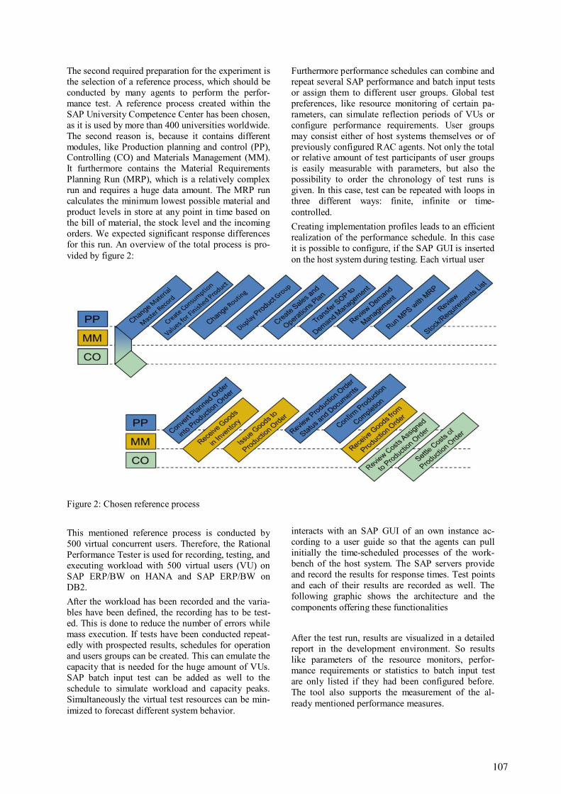
The second required preparation for the experiment is the selection of a reference process, which should be conducted by many agents to perform the perfor-mance test. A reference process created within the SAP University Competence Center has been chosen, as it is used by more than 400 universities worldwide. The second reason is, because it contains different modules, like Production planning and control (PP), Controlling (CO) and Materials Management (MM). It furthermore contains the Material Requirements Planning Run (MRP), which is a relatively complex run and requires a huge data amount. The MRP run calculates the minimum lowest possible material and product levels in store at any point in time based on the bill of material, the stock level and the incoming orders. We expected significant response differences for this run. An overview of the total process is pro-vided by figure 2:

Figure 2: Chosen reference process This mentioned reference process is conducted by 500 virtual concurrent users. Therefore, the Rational Performance Tester is used for recording, testing, and executing workload with 500 virtual users (VU) on SAP ERP/BW on HANA and SAP ERP/BW on DB2. After the workload has been recorded and the varia-bles have been defined, the recording has to be test-ed. This is done to reduce the number of errors while mass execution. If tests have been conducted repeat-edly with prospected results, schedules for operation and users groups can be created. This can emulate the capacity that is needed for the huge amount of VUs. SAP batch input test can be added as well to the schedule to simulate workload and capacity peaks. Simultaneously the virtual test resources can be min-imized to forecast different system behavior.

Furthermore performance schedules can combine and repeat several SAP performance and batch input tests or assign them to different user groups. Global test preferences, like resource monitoring of certain pa-rameters, can simulate reflection periods of VUs or configure performance requirements. User groups may consist either of host systems themselves or of previously configured RAC agents. Not only the total or relative amount of test participants of user groups is easily measurable with parameters, but also the possibility to order the chronology of test runs is given. In this case, test can be repeated with loops in three different ways: finite, infinite or time-controlled. Creating implementation profiles leads to an efficient realization of the performance schedule. In this case it is possible to configure, if the SAP GUI is inserted on the host system during testing. Each virtual user

interacts with an SAP GUI of an own instance ac-cording to a user guide so that the agents can pull initially the time-scheduled processes of the work-bench of the host system. The SAP servers provide and record the results for response times. Test points and each of their results are recorded as well. The following graphic shows the architecture and the components offering these functionalities

After the test run, results are visualized in a detailed report in the development environment. So results like parameters of the resource monitors, perfor-mance requirements or statistics to batch input test are only listed if they had been configured before. The tool also supports the measurement of the al-ready mentioned performance measures.

107

As there are still some issues with the data import, the test on ERP on HANA with the GBI dataset has not been conducted yet on the ERP/BW on HANA system.

Figure 3: Overview of the Rational Performance Tester Architecture

3.4 Second Phase: Allocation of the Sys-tems

The first step was the migration of an existing SAP ERP on HANA and an SAP BW on HANA system including the necessary datasets for the intended workload. This was planned to be done using the heterogeneous SAP system copy procedure. One prerequisite for doing so is an upgrade to SAP en-hancement package 6 (EhP 6). Due to problems with the upgrade of SAP IDES systems, we decided to focus on the SAP ERP system with Global Bike Inc. (GBI) dataset. GBI is an exemplary dataset, of a

company with a use case similar to IDES. The up-grade and export of this system showed neither errors nor further problems. However, during the import phase on the HANA database severe errors in four

packages occurred. The log files are being analyzed further at this point, but no solution to this problem has been found yet.

4 Conclusion

The goal of this study was to test the load perfor-mance of an ERP/BW system on HANA in compari-son to the same system running on a relational data-base. The first step was to create a reference frame-

108

work to identify which KPIs were only related to database behavior, as well as to create a reference process which will be conducted by many virtual users on the different systems. The reference frame-work contains the KPIs: request time (ms), DB Proc Calls, Enqueue Time and Commit Time. As a refer-ence process for the ERP system a typical production planning process was selected, as it includes different modules, as well as the MRP run. The MRP run is a complex calculation of required material at different point in times and needs a huge data amount. The next step was the system copy to migrate the SAP ERP on HANA. Therefore, the ERP software had to be updated to the latest enhancement package (EhP) first. Errors regarding the upgrade and the export phase were resolved successfully. However, there are still some issues with the import phase of the ERP system with an exemplary dataset (GBI). As these errors are not resolved yet, we applied for a further project within the HPI Future SOC Lab to be able to reach our project goals.

5 References

[1] IDC (2012): IDC-Studie: Big Data in

Deutschland 2012 - Unternehmen stehen noch ganz am Anfang. http://www.idc.de/press/presse_idc-studie_big_data2012.jsp, accessed at 01.02.2013.

[2] Plattner, H.; Zeier, A. (2011): In-Memory Data Management: An Inflection Point for En-terprise Applications, Springer 2011.

[3] Loos, P.; Lechtenbörger, J.; Vossen, G.; Zeier, A.; Krüger, J.; Müller, J.; Lehner, W.; Koss-mann, D.; Fabian, B.; Günther, O. (2011): In-Memory-Datenmanagement in betrieblichen Anwendungssystemen. In: Wirtschaftsinfor-matik, Vol. 6 (2011) No. 53, pp. 383-390.

[4] Loos, P.; Strohmeier, S.; Piller, G.; Schütte, R. (2012): Kommentare zu „In-Memory-Datenmanagement in betrieblichen Anwen-dungssystemen". In: Wirtschaftsinformatik, Vol. 54 (2012) No. 4, pp. 209-213.

[5] Stonebraker, M. (2011): Stonebraker on Data Warehouses. In: Communications of the ACM, Vol. 54 (2011) No. 5, pp. 10-11.

[6] Kemper, A.; Neumann, T. (2010): HyPer: HYbrid OLTP&OLAP High PERformance Database System. Institute of Computer Sci-ence, 2010.

[7] Strohmeier, S. (2012): Hauptspeicherdaten-banken in der betrieblichen Informationsver-sorgung - Technische Innovation und fachli-che Stagnation? In: Wirtschaftsinformatik, Vol. 54 (2012) No. 4, pp. 209-210.

109

Using Thread-Level Speculation to Enhance JavaScript Performance inWeb Applications

Jan Kasper Martinsen and Hakan GrahnSchool of Computing

Blekinge Institute of TechnologySE-371 79 Karlskrona, Sweden

{Jan.Kasper.Martinsen,Hakan.Grahn}@bth.se

Anders IsbergSony Mobile Communications AB

SE-221 88 Lund, [email protected]

Abstract

We have implemented Thread-Level Speculation in theSquirrelfish JavaScript engine, which is part of the We-bKit browser environment. We were able to speed upthe execution time by a factor of up to 8.4 times com-pared to the sequential version for 15 very popularweb applications on an 8-core computer, without mak-ing any modifications to the JavaScript source code.The results also show that we probably could take ad-vantage of an even higher number of cores.

1 Introduction

JavaScript [3] is a dynamically typed, object-basedscripting language where the JavaScript code is com-piled to bytecode instructions at runtime which in turnare interpreted in a JavaScript engine [2, 14, 9].One of the most common uses for JavaScript is for in-teractivity to the client side of web applications. Mod-ern web applications are complex networks of coderunning on multiple servers and in the client-side webbrowser. Our intention with this work is to speed upthe client-side execution.Several JavaScript optimization techniques and bench-marks have been suggested, but these benchmarkshave been reported as unrepresentative for JavaScriptexecution in web applications [11, 12, 5]. One im-portant result of this, is that the popular optimiza-tion technique just-in-time compilation (JIT) wherethe JavaScript code first is compiled, then executedas native code decrease the execution time for a setof JavaScript benchmarks, while it at the same timeincreases JavaScript execution time for popular webapplications [6].JavaScript is a sequential programming language andcannot take advantage of multicore processors. For-tuna et al. [1] showed that there exists significant po-tential parallelism in many web applications with a po-tential speedup up to 45 times compared to the sequen-tial execution. However, they did not implement sup-

port for parallel execution in any JavaScript engine.Web Workers [13] allows parallel execution of tasks inweb applications, but it is the programmer’s responsi-bility to extract and express the parallelism. In addi-tion, Web Workers aim is to increase the responsivityof a web application, rather to improve the executionspeed of JavaScript execution.To hide the details of the underlying hardware, oneapproach is to dynamically extract parallelism froma sequential program using Thread-Level Specula-tion (TLS). The performance potential of TLS hasbeen shown for applications with static loops, stat-ically typed languages, in Java bytecode environ-ments, and there have been some initial attempts forJavaScript [4].In [8] we demonstrated an up to 8 times speedup oversequential execution time for 15 very popular webapplications [10] on a dual quadcore computer witha TLS enabled Squirrelfish [14] used in the WebKitbrowser environment. The execution and behaviourof a web application is dependent not only on theJavaScript engine itself, but also on the interaction be-tween JavaScript and the web browser such as manip-ulation of the Document Object Model (DOM) tree.However, we deliberately focused on the JavaScriptaspect.As we mentioned earlier, Fortuna et al. [1] showed thatthere exists a 45 times speedup for web applications,therefore we are interested in how well our findingscould scale with a larger number of cores.

2 Current Results

In Figure 1 we have measured the speedup withThread-Level Speculation(TLS) and Just-in-time com-pilation (JIT) on a set of very popular web applica-tions. The results indicate that:

• TLS always decreases the execution time

• The Squirrelfish JIT based engine increases theexecution time for 10 out of 15 cases (similar tothe results in [7])

111

• The Google V8 JIT engine increases the execu-tion time for 8 out of 15 cases

The results in Table 1 show that the maximum num-ber of threads is higher for 14 out 15 use cases, thanthe number of cores in order dual quad core computer.Therefore there could be a potential to improve execu-tion speed further with a larger number of cores.Both the Thread-Level Speculation execution time re-sults in Figure 1 and Table 1 follows the postulationof Fortuna et al. [1], that there exists a significant po-tential for parallelism in web applications. There arenumerous reasons for this; first that, JavaScript in webapplications makes many function calls. These func-tion calls are often events called from the web appli-cation, and they are often anonymous function. Thesefunctions are often independent to one another (i.e., donot write or read to the same global variable and returnany values), which makes them very suitable for beingexecuted in parallel. Thread-Level Speculation is onetechnique for doing this, which is suggested in [8].Our Thread-Level Speculation experiments have beenperformed on a a dual quad core computer, so thereis a limit to how much extracted parallelism this com-puter can take do. However, interestingly in web ap-plications, we are not lacking of parallelism to takeadvantage of (Table 1 shows many speculations andfew rollbacks). What we are currently missing, is acomputer with even more cores. Another interestingfeature is that this parallel potential is perhaps not thenormal applications, where parallelism is used.In this respect, the Hasso-Plattner institute gave usaccess to a computer with 48 cores. We are in theprogress of understanding if an increased number ofavailable cores can be used to take advantage of theparallelism of web application, or if there are otherfactors (of for instance more architectural nature or theexecution characteristics in web applications) that pre-vents us from taking advantage of the large number ofcores.

3 Future research

There is a potential to increase the speedup withThread-Level Speculation, and it would be very inter-esting to see on a larger number of cores, as the mea-surements suggests that we could take advantage formore cores. One extension we will do in future stud-ies is that we want to extends the number of use casesfor the web application, to make them both larger andstudy their use with a larger number of users.Therefore we hope to continue to have access toHasso-Plattner Institute’s wide selection of computers,to future understand the factors of execution of theseuse cases on a large number of cores, and collaboratewith Hasso-Plattner for future and even more interest-ing results.

References

[1] E. Fortuna, O. Anderson, L. Ceze, and S. Eggers. Alimit study of javascript parallelism. In 2010 IEEEInt’l Symp. on Workload Characterization (IISWC),pages 1–10, Dec. 2010.

[2] Google. V8 JavaScript Engine, 2012. http://code.google.com/p/v8/.

[3] JavaScript. http://en.wikipedia.org/wiki/JavaScript, 2010.

[4] J. K. Martinsen and H. Grahn. An alternative opti-mization technique for JavaScript engines. In ThirdSwedish Workshop on Multi-Core Computing (MCC-10), pages 155–160, November 2010.

[5] J. K. Martinsen and H. Grahn. A methodology forevaluating JavaScript execution behavior in interactiveweb applications. In Proc. of the 9th ACS/IEEE Int’lConf. On Computer Systems And Applications, pages241–248, December 2011.

[6] J. K. Martinsen, H. Grahn, and A. Isberg. A com-parative evaluation of JavaScript execution behavior.In Proc. of the 11th Int’l Conf. on Web Engineering(ICWE 2011), pages 399–402, June 2011.

[7] J. K. Martinsen, H. Grahn, and A. Isberg. Evaluat-ing four aspects of JavaScript execution behavior inbenchmarks and web applications. Research Report2011:03, Blekinge Institute of Technology, July 2011.

[8] J. K. Martinsen, H. Grahn, and A. Isberg. Using specu-lation to enhance javascript performance in web appli-cations. IEEE Internet Computing, 17(2):10–19, 2013.

[9] Mozilla. SpiderMonkey – Mozilla Developer Net-work, 2012. https://developer.mozilla.org/en/SpiderMonkey/.

[10] G. R. Notess. Alexa: Web archive, advisor, and statis-tician. Online, 22(3):29–30, 1998.

[11] P. Ratanaworabhan, B. Livshits, and B. G. Zorn. JS-Meter: Comparing the behavior of JavaScript bench-marks with real web applications. In WebApps’10:Proc. of the 2010 USENIX Conf. on Web ApplicationDevelopment, pages 3–3, 2010.

[12] G. Richards, S. Lebresne, B. Burg, and J. Vitek. Ananalysis of the dynamic behavior of JavaScript pro-grams. In PLDI ’10: Proc. of the 2010 ACM SIG-PLAN Conf. on Programming Language Design andImplementation, pages 1–12, 2010.

[13] W3C. Web Workers — W3C Working Draft 01September 2011, Sep. 2011. http://www.w3.org/TR/workers/.

[14] WebKit. The WebKit open source project, 2012.http://www.webkit.org/.

112

0

1

2

3

4

5

6

7

8

9

Google (0.72)

Facebook (0.53)

YouTube (0.12)

Wikipedia (0.50)

BlogSpot (0.22)

MSN

(0.43)

Linkedin (0.54)

Amazon (0.98)

WordPress (0.26)

Ebay (0.43)

Bing (0.74)

Imdb (0.36)

Myspace (0.37)

BBC (0.87)

Gm

ail (0.65)

SP

EE

DU

P

Thread-Level SpeculationJust-in-time compilation (jsc)

google v8 (Chromium)

Figure 1: JavaScript execution speedup over the interpreted sequential JavaScript engine for the 15 web applications when TLS is enabled, when just-in-time compilation is enabled and for the Google V8 JIT engine in the chromium web browser. We have written the exe-cution time of TLS relative to the sequential execution time in parenthesis after the name of the web applications.

Application Number of Number of Speculations / Maximum number Max speculation Average Memoryspeculations rollbacks Rollbacks of threads depth depth usage (MB)

Amazon 10768 267 40.31 83 23 8.0 14.1BBC 6392 154 41.51 117 14 5.12 33.0Bing 303 18 16.83 30 7 2.22 1.4Blogspot 778 15 51.87 16 14 2.16 1.6Ebay 7140 101 70.69 63 15 5.33 27.0Facebook 968 51 18.98 27 22 9.16 7.1Gmail 1193 19 62.79 34 10 2.68 1.95Google 1282 36 35.61 40 10 3.9 5.5Imdb 5300 156 33.97 54 24 6.85 17.8LinkedIn 1815 51 35.59 36 11 2.27 7.1MSN 12012 133 90.32 191 24 5.85 20.1Myspace 3679 93 39.56 39 14 5.54 17.4Wordpress 5852 63 92.89 63 99 4.55 9.7Wikipedia 12 0 undefined 8 4 0 1.1YouTube 7349 25 293.96 407 13 5.44 17.1

Table 1: Number of speculations, number of rollbacks, relationship between rollbacks and speculations, maximum number of threads, maximum nested speculation depth, average depth for recursive search when deleting values associated with previous speculations, and average memory usage before each rollback (in megabytes).

113

Forecasting of Energy Load Demand and Energy Production fromRenewable Sources using In-Memory Computing

– Project Report –

Witold Abramowicz Tomasz Rudny Monika Kaczmarek

Department of Information SystemsFaculty of Informatics and Electronic Economy

Poznan University of EconomicsAl. Niepodleglosci 10, 61-875 Poznan

[email protected]

Abstract

This report presents the short overview of the initia-tives undertaken in the field of forecasting of energyload demand and energy production using the com-putational power of SAP HANA. One of the researchhypothesis that we focused on, was that the forecast-ing of demand can be done in quasi-real time, evenif conforming to bottom-up approach, i.e., computingseparate forecasts for each customer. The report pro-vides information on the project main objectives, usedHPI Future SOC Lab resources, findings as well asnext steps envisioned.

1 Introduction

The vast amount of data that organizations shouldgather, store and process, entails a set of new require-ments towards the analytical solutions used by orga-nizations. These requirements have become driversfor the development of the in-memory computingparadigm [4], which enables the creation of applica-tions running advanced queries and performing com-plex transactions on very large sets of data in a muchfaster and scalable way than the traditional solutions.The main aim of our work is to examine the analyticalpossibilities of the in-memory computing solution, onthe example of SAP HANA, and their possible appli-cations. In order to do that we apply SAP HANA andits components to the challenge of forecasting of theenergy demand and production in the energy sector.Within this report we focus on the forecasting of en-ergy load demand. Forecasting energy demand in realtime as well as creation of models featuring a low pre-diction error is extremely difficult [7]. Therefore, sucha scenario requires a solution that supports fast opera-

tions on a very large number of data and is equipped with adequate analytical modules. These requirements correspond to SAP HANA.As shown by many researchers and practitioners en-ergy load forecasting can be done more accurately, if forecasts are calculated for all customers separately and then combined via bottom-up strategy to produce the total load forecast [2, 3]. Also, additional im-provement is expected, if different models and param-eters can be tested quickly to provide the best model selection capability. Quasi real time load forecasting could lead to substantial savings for companies and also for the environment, up till now however, it was computationally difficult, as for a typical energy seller a number of residential customers exceeds hundreds of thousands.

2 Project Aims

The goal of the presented project was to design andimplement quasi real-time load forecasting for a hugenumber of individual customers profiles using in mem-ory computing. We formulated a hypothesis: forecast-ing accuracy (which is directly related to costs) canbe substantially increased by individual forecasting onthe level of each customer done in quasi real-time us-ing SAP HANA parallelism, and a new insight into theanalysed data can be gained.Throughout the project we aimed at building an an-alytical system using SAP HANA for support of En-ergy Load Demand Forecasting. Every energy sellingcompany must accurately predict the load demand inorder to prepare - either by own generation resourcesor by buying on the long and short term market - thesupply. Our aim was to evaluate whether SAP HANAanalytical capabilities can augment the classical meth-ods of forecasting. On the other hand, we wanted

115

Figure 1: Comparison of the energy load demand of two exemplary users

to check if the outstanding processing power of SAPHANA can lead to new concepts and methods of fore-casting. Here, we relied on the bottom-up approach,which has rarely been used till now, also because ofthe lack of computation power strong enough to har-ness thousands of time series.Apart of forecasting our aim was to check how SAPHANA can support daily business analytic task of en-ergy companies for example contract preparation. Oneof the most important tasks involved is finding a cus-tomer profile most similar to the prospect customer,thus fitting the tariff. But since comparisons of de-mand profile are very expensive in terms of computa-tions, here we saw another place for potential use ofSAP HANA.To achieve our aims we organized the work into thefollowing steps:

1. Designing and setting-up of a database optimizedfor storage of massive historical load data as wellas predictive analysis.

2. Cleansing the data and remove missing values byimputation,

3. Implementing different forecasting strategiesbased on the bottom-up approach.

4. Testing different forecasting models and exoge-nous variables.

5. Calculating many forecasts for the same time se-ries data using different parameters and models.

6. Comparing the models to choose the best set-tings.

We hoped that with the parallel processing and SAPHANA libraries to calculate load demand forecasts,by keeping data in-memory, which will eliminate thecostly data transfer from hard drives into memory,which has been one of the key inhibitions of classi-cal analytical software, we will be able to prove thatnew approach to demand forecasting is now possible.

3 Future SOC Lab Resources Used

During the project we used SAP HANA Studio and the assigned instance (12) combined with Rserve for pre-dictive analyses. SAP HANA offers a way to incor-porate the R code directly into the SQL Script [6, 1]. Table variables can be passed on as input parameters, while output parameters can receive values of R data frames. This makes it possible to conveniently use R packages and procedures directly from SAP HANA. Throughout the project we uploaded the data into SAP HANA as column tables. Then, we rearranged the data for our experiments, creating auxiliary tables and columns. Because the data we obtained from a major Polish energy distributor consisted of only a limited number of times series, we decided to generate arti-ficial data as randomization of the existing o ne. The randomization modified the values of the energy load demand by 10%. It was performed using the R script procedure.The experiments and analysis of individual user pro-files have shown that indeed, the characteristics of ag-gregated and individual profiles are different, e.g., they have different shapes, and in addition, that the pro-files of individual users also differ among each other. As shown on Figure 1 - both individual profiles show peaks in the morning and evenings, but the shape of the second user vary for different days of the week and parts of the year whereas the first user exhibits a more or less constant energy load demand irrespectively of the day of a week. The individual electricity load pro-file is influenced by the number of factors, which may be divided in the following categories [3]: (1) elec-tricity demand variations between customers, (2) sea-sonal electricity demand effects, (3) intra-daily varia-tions, and (4) diurnal variations in electricity demand. The influence of those factors is specific for groups of customers (having similar profiles).Within the phase of our project addressed by this re-port, we focused on using SAP HANA Predictive Analysis Library (PAL) [5] both to build univariate time series forecasting models and to build more ad-vanced regression models (see Figure 2).The following experiments were run on SAP HANA

116

Figure 2: Prognosis of energy load demand using the regression model

using the aforementioned resources:

• Computing the summary forecast by summing allindividual time series and calculating the (single)forecast over the summarized data,

• Calculating individual forecasts for all customers,then summarizing the forecasted values to com-pute the summary forecast,

• Comparing the forecasting error between differ-ent scenarios,

• Comparing different forecasting models - amongothers Holt-Winters exponential smoothing (sin-gle and double) and linear regression.

The experiments conducted so far focused on evaluat-ing SAP HANA capabilities for time series forecast-ing, data manipulation and storage, as well as organiz-ing the code.We also had to impute the data as sometimes the valueof the historical energy load demand was missing. Theimputation code is presented below:

CREATE PROCEDURE IMPUTE_MISSING(IN x"totals",OUT y "totals_imputed")LANGUAGE RLANG AS BEGINmissing <- is.na(x$value)n.missing <- sum(missing)x.obs <- x$value[!missing]imputed <- ximputed$value[missing] <-sample(x.obs, n.missing, replace=TRUE)y <- as.data.frame(imputed)END;

As already indicated, within the first steps of the researchwe assigned our focus to the conducting experiments usingR. We were able to generate forecasts using various modelsbased on 180 days historical data with a 14 days horizon.The models tested included ARIMA and Holt-Winters expo-nential smoothing. The code for forecasting can be nicelyand neatly written in R as shown on the example of Holt-Winters exponential smoothing:

CREATE PROCEDURE FS_STEP(IN x "input2",IN temp "temp", OUT y "totals_forecast")LANGUAGE RLANG ASBEGINts1 <- ts(x$value, frequency=24)m <- HoltWinters(ts1)f <- predict(m, n.ahead=14*24)

forecast <- f[1:14*24]

y <- as.data.frame(cbind(temp, forecast))END;

In turn, data preparation in PAL was straightforward like inthis example:

DROP table TEMP_REG_DATA_01;CREATE column tableTEMP_REG_DATA_01("ID" INTEGER,"VALUE" DOUBLE, "WDAY" INTEGER,"H" INTEGER, "TEMPERATURE" DOUBLE,"FORECAST" DOUBLE);

INSERT INTO TEMP_REG_DATA_01(SELECT DISTINCT(DAYOFYEAR("data")-1)*24+"h"AS "ID", "value" AS "VALUE",WEEKDAY("data") AS "WDAY", "h" AS "H","temperature" AS "TEMPERATURE","forecast" AS "FORECAST"FROM "eda2" WHERE "uid" = 1 ORDER BY "ID");

Much to our surprise, the setting up of PAL engine for linearregression did not require special efforts and can be done infew simple, standard steps which can be then reused whenneeded.

DROP TYPE PAL_T_RG_DATA;CREATE TYPE PAL_T_RG_DATA AS TABLE("ID" INTEGER, "VALUE" DOUBLE,"WDAY" INTEGER, "H" INTEGER,"TEMPERATURE" DOUBLE);

117

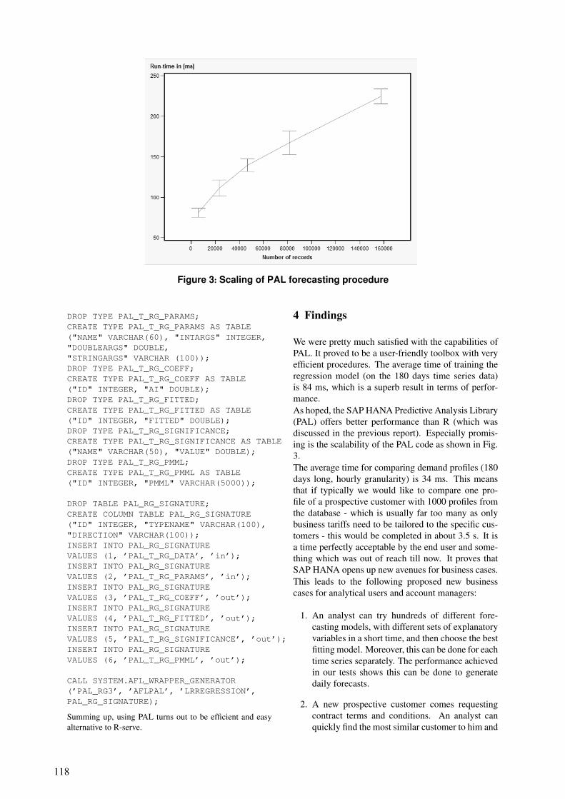
Figure 3: Scaling of PAL forecasting procedure

DROP TYPE PAL_T_RG_PARAMS;CREATE TYPE PAL_T_RG_PARAMS AS TABLE("NAME" VARCHAR(60), "INTARGS" INTEGER,"DOUBLEARGS" DOUBLE,"STRINGARGS" VARCHAR (100));DROP TYPE PAL_T_RG_COEFF;CREATE TYPE PAL_T_RG_COEFF AS TABLE("ID" INTEGER, "AI" DOUBLE);DROP TYPE PAL_T_RG_FITTED;CREATE TYPE PAL_T_RG_FITTED AS TABLE("ID" INTEGER, "FITTED" DOUBLE);DROP TYPE PAL_T_RG_SIGNIFICANCE;CREATE TYPE PAL_T_RG_SIGNIFICANCE AS TABLE("NAME" VARCHAR(50), "VALUE" DOUBLE);DROP TYPE PAL_T_RG_PMML;CREATE TYPE PAL_T_RG_PMML AS TABLE("ID" INTEGER, "PMML" VARCHAR(5000));

DROP TABLE PAL_RG_SIGNATURE;CREATE COLUMN TABLE PAL_RG_SIGNATURE("ID" INTEGER, "TYPENAME" VARCHAR(100),"DIRECTION" VARCHAR(100));INSERT INTO PAL_RG_SIGNATUREVALUES (1, ’PAL_T_RG_DATA’, ’in’);INSERT INTO PAL_RG_SIGNATUREVALUES (2, ’PAL_T_RG_PARAMS’, ’in’);INSERT INTO PAL_RG_SIGNATUREVALUES (3, ’PAL_T_RG_COEFF’, ’out’);INSERT INTO PAL_RG_SIGNATUREVALUES (4, ’PAL_T_RG_FITTED’, ’out’);INSERT INTO PAL_RG_SIGNATUREVALUES (5, ’PAL_T_RG_SIGNIFICANCE’, ’out’);INSERT INTO PAL_RG_SIGNATUREVALUES (6, ’PAL_T_RG_PMML’, ’out’);

CALL SYSTEM.AFL_WRAPPER_GENERATOR(’PAL_RG3’, ’AFLPAL’, ’LRREGRESSION’,PAL_RG_SIGNATURE);

Summing up, using PAL turns out to be efficient and easyalternative to R-serve.

4 Findings

We were pretty much satisfied with the capabilities ofPAL. It proved to be a user-friendly toolbox with veryefficient procedures. The average time of training theregression model (on the 180 days time series data)is 84 ms, which is a superb result in terms of perfor-mance.As hoped, the SAP HANA Predictive Analysis Library(PAL) offers better performance than R (which wasdiscussed in the previous report). Especially promis-ing is the scalability of the PAL code as shown in Fig.3.The average time for comparing demand profiles (180days long, hourly granularity) is 34 ms. This meansthat if typically we would like to compare one pro-file of a prospective customer with 1000 profiles fromthe database - which is usually far too many as onlybusiness tariffs need to be tailored to the specific cus-tomers - this would be completed in about 3.5 s. It isa time perfectly acceptable by the end user and some-thing which was out of reach till now. It proves thatSAP HANA opens up new avenues for business cases.This leads to the following proposed new businesscases for analytical users and account managers:

1. An analyst can try hundreds of different fore-casting models, with different sets of explanatoryvariables in a short time, and then choose the bestfitting model. Moreover, this can be done for eachtime series separately. The performance achievedin our tests shows this can be done to generatedaily forecasts.

2. A new prospective customer comes requestingcontract terms and conditions. An analyst canquickly find the most similar customer to him and

118

then customize the tariff based on what is alreadyknown for the existing similar customer. This canlead to substantial savings and better tariff opti-mization.

3. Demand forecasts can be generated for individ-ual customers which will play an important rolewhen smart grids based on renewable sources be-come more popular.

5 Conclusions and Next Steps

The goal of the presented project was to design andimplement quasi real-time load forecasting for a hugenumber of individual customers profiles using in mem-ory computing. We proved a hypothesis: forecastingaccuracy can be substantially increased by individualforecasting on the level of each customer done in quasireal-time using SAP HANA parallelism, and a new in-sight into the analysed data can be gained.Within the project we evaluated efficiency and perfor-mance of various computational strategies. Fast com-putations allowed for comparisons of different fore-casting models and choosing the best one on a spot.Also, the possibility for adding different exogenousvariables to the models and being able to quickly anal-yse their significance opened up new applications ofenergy load forecasting.An additional intermediate result achieved is the pos-sibility to cluster customers for the purpose of pricingand marketing campaign management. Thanks to SAPHANA huge computational powers it became possibleto compare models in quasi-real time, select the mostsignificant variables and provide new ways of analysis.The achieved results include a significant speed-up ofthe forecasting process and accuracy improvement.With the analytical and computational experimentsconducted we are now ready to put all those blockstogether and utilize the reporting capabilities of SAPHANA to build a prototype of a system which busi-ness users could use to support their daily activities.So the next steps would be: Building a prototype ofa system supporting business users in energy demandforecasting.

References

[1] Y. Aragon. Series temporelles avec R. Methodes et cas.Springer, Collection Pratique R, 1st edition, 2011.

[2] W. Charytoniuk, M.-S. S. Chen, P. Kotas, andP. Van Olinda. Demand forecasting in power distri-bution systems using nonparametric probability den-sity estimation. Power Systems, IEEE Transactions,14/4:1200–1206, 1999.

[3] F. McLoughlin, A. Duffy, and M. Conlon. Evaluationof time series techniques to characterise domestic elec-tricity demand. Energy, 50(0):120 – 130, 2013.

[4] H. Plattner and A. Zeier. In-Memory Data Manage-ment: An Inflection Point for Enterprise Applications.Springer, Berlin Heidelberg, 2011.

[5] SAP. SAP HANA Predictive Analysis Library (PAL)Reference. 2012.

[6] SAP. SAP HANA R Integration Guide. 2013.[7] R. Weron. Modeling and Forecasting Electricity Loads

and Prices: A Statistical Approach. John Wiley andSons Ltd., 2006.

119

Normalisation of Log MessagesReport for Project “Towards an Integrated Platform for Simulating, Monitoring, and Analytics of SAP

Software” in 2013 Spring at HPI FutureSoC Lab

Andrey Sapegin, David Jaeger, Amir Azodi, Feng Cheng, Christoph MeinelHasso-Plattner-Institut (HPI), University of Potsdam

P.O.Box 900460, 14440 Potsdam, Germany{andrey.sapegin, david.jaeger, amir.azodi, feng.cheng, christoph.meinel}@hpi.uni-potsdam.de

Abstract—The differences in log file formats employed in avariety of services and applications remain to be a problem forsecurity analysts and developers of intrusion detection systems.The proposed solution, i.e., the usage of common log formats,has a limited utilization within existing solutions for securitymanagement. In our paper, we reveal the reasons for this limita-tion. We show disadvantages of existing common log formats fornormalisation of security events. To deal with it we have createda new log format that fits for intrusion detection purposes andcan be extended easily. Taking previous work into account, wewould like to propose a new format as an extension to existingcommon log formats, rather than a standalone specification.

Keywords—log normalisation, intrusion detection, common logformat

I INTRODUCTION

Nowadays, every application has its own log file format.Such a variety of formats complicates log analysis [1] andcauses problems for system administrators, developers of in-trusion detection systems (IDS) [2] and security analysts [3].

Therefore, several solutions [4] were introduced with theaim to solve this problem: CEE [3], CEF [5], IODEF [6].

However, there are many developers who avoid using com-mon log formats in their projects. This statement particularly applies to intrusion detection systems. Many software vendors and open source projects still use their own log format for IDSs [7, 8, 9]. The reasons for this situation hide in the IDS architecture. To operate rapidly, such systems need to analyse huge amount of logs from hundreds of devices and services on the fly. T herefore, t he l og f ormat s hould b e lightweight and able to encapsulate all network and host logs from large datasets.

Log file standards that are aiming to handle all possible log output of any service, do not fit for these purposes. Moreover, in some cases, the variety of standardised fields, o ffered by such a common log file f ormat, d o n ot p rovide a suitable schema for normalisation and correlation of security events. During the development of our own IDS —Security Analytics Lab [10] — we have faced the same challenges and came to the same solution: a log format that is specially designed for IDSs. However, the object log format we present in this paper noticeably differs from the existing solutions.

Our goal was to experiment with a flexible lightweightformat to optimise attack detection. First, we analysed a varietyof large log files and came up with a list of common fields thatcan be found in the logged events. Then, this list was reduced

to the fields that we considered most important for the securityanalysis of occurred events.

As a result, the developed log format facilitates the detec-tion of attacks and simplifies their correlation. We demonstratethe ability of our format to simplify attack detection within acase study. Besides this particular use case, the proposed logformat retains to be adjustable and could be utilised for genericnormalisation concepts.

The remainder of the paper has the following structure:Section II provides overview of the Future SOC Lab project,Section III describes the data set used, Section IV evaluatesand compares existing log formats, Section V provides detailson the log format we developed, Section VI tells about resultsof a case study. We discuss our results and conclude in theSection VII.

II HPI FUTURE SOC LAB PROJECT

The research result described in this report is part of ourHPI Future SOC Lab project “Towards an Integrated Platformfor Simulating, Monitoring, and Analytics of SAP Software”.Within this project we expect to design and implement a multi-purpose platform with complex software, e.g., SAP software.This platform will be used as a base for vulnerability analysisresearch in simulated enterprise environment. To carry it out,we are testing the known and modern attack approaches andalso attract external attackers using self-organised honeypotsystem. Each component of the platform should be connectedto the centralised monitoring and security management system,which collects data, that could be used for different researchdirections also after the project ends. The project was plannedin three phases:

• design, development and deployment of SAL-monitored SAP platform

• research, design and implementation of Attacks andHoneypots of SAP software

• creation of use and attack scenarios, scientific analysisof results and data collected

The first phase concentrates on the preparation of theplatform, research and selection of tools and technologies. Weselect typical distributions of SAP software, install, configurethem and prepare the connection to the Security Informationand Event Management System (SIEM). At the same stepwe prepare other components of the system and developthe platform architecture. The second step is focused on the

121

vulnerability analysis of software deployed on the platform.We select tools for penetration testing, analyse known anddiscover unknown vulnerabilities. Meanwhile we explore ex-isting attacking approaches and research for new attacks. Forthe last phase we propose more detailed analysis of collecteddata, improvement of the platform and security managementsystem, as well as the documentation, white papers withtechnical details and vulnerability reports. In the end weplan to deliver the stable prototype of the platform, includinghoneypot system, monitoring and intrusion detection systems,as well as actual SAP software, for which we will report allfound previously unknown vulnerabilities. All tested attacktools and approaches will be documented and presented in therepository together with the documentation of project conceptsand technical reports.

We have carried out the first phase of the project in thespring and summer 2013. During this phase we have designeda test bed for vulnerability analysis with SAP software andHPI Security Analytics Lab (HPI-SAL) — our own developedSIEM, based on SAP HANA in-memory database [10]. Theuse of SIEM implies the ability to collect, process and correlatelog messages from all monitored software. Variety of differentlog formats and message types oblige the intrusion detectionsystem to be able to normalise all the events being producedinto the same format. The normalisation process is one ofthe most challenging tasks for the modern intrusion detectionsystems. HPI Security Analytics Lab should not only convertthe messages in the same format, but also recognise (and putin the different fields) the meaningful parts of log messages,extracting the semantics of the event details for posteriorcorrelation. To deal with this problem we have developed ourown log format for the normalisation of any types of logmessages. The proposed format has a number of advantages —we describe them in this report — if compared with existingsolutions.

Another challenging task we have faced during the firstphase is a vulnerability modelling. To design different platformcomponents, such as honeypot or develop the penetrationtesting strategy, it is extremely important to gather informationabout vulnerable software, collect details and classify newlydiscovered vulnerabilities. We have solved this problem andused the separate database that acts as an integrated storagefor all existing vulnerability information: the HPI Vulnera-bility Database (HPI-VDB) [11]. HPI-VDB is a repositorycontaining structured information about almost 60000 vulner-abilities, including the description of pre- and post-conditionsfor every vulnerability. We use these data to conduct researchon information quality, new services and classification ofvulnerabilities. During the first phase we were working onthe further development of HPI-VDB and connection to HPISecurity Analytics Lab. Our goal is to embed the HPI-VDBinto the platform and integrate it into the framework forthe vulnerability analysis of SAP Software. During the nextphase we will use it as information source while discovering,evaluating and classifying vulnerabilities of selected software.

The prototype of the platform described above will allowus to perform vulnerability analysis and penetration testing ofSAP software, as well as discover new attack vectors throughthe honeypot system, which are the next steps in the project.

III DATA

To prove our concepts, we utilised data from “Scan of theMonth” Honeynet [12] Challenge: “Scan 34 - Analyze realhoneynet logs for attacks and activity” [13]. The HoneynetProject aims to help security specialists to sharpen their foren-sics and attack detection skills. To achieve it, the project sharesreal attack data collected from honeynets from all over theworld. The “Scan of the Month” challenge provides archiveswith log files from different hardware and software systems forthe postmortem analysis. The “Scan 34” challenge containslog files being collected between 30 January and 31 March2005. We chose this particular challenge because it impliesanalysis of multiple log files for different services and includesvarious heterogeneous attack traces. We describe the log filesin Table I.

The “Scan 34” challenge also provides the description onthe attacks and important events in the log files. See the detailsof the 15 most important events in Table II.

In total, four attacks led to the server’s compromisation.Two of four attackers used the vulnerability of ‘awstats.pl’installed after the server reboot, probably by a system admin-istrator. Another two attackers successfully brute-forced theSSH password. The first attacker has also installed an IRC botright after the intrusion. Other events listed in the table werenot harmful for the server; they represent suspicious activitythat did not result into a successful intrusion.

IV EXISTING LOG FORMATS FOR NORMALISATION OFSECURITY EVENTS

Before we decided to use our own log format, we haveevaluated existing solutions, trying to estimate if they couldfit for our purposes of normalisation of security events. Pleasesee the overview of proposed log formats in Table III.

The selected formats have different structure, size andeven usage purpose. CEE is a generic format for loggingany types of events, IDMEF was developed for exchange ofsecurity messages. IODEF is specially designed for computersecurity incidents, as well as CEF developed as a part ofintrusion detection system. Although the described formatshave different purposes, each of them could be used for lognormalisation.

However, not every part of the log message could benormalised to the standard fields defined in every format. Todeal with it, each format allows to use extra fields or extend itsstructure. Therefore we decided to check how many changeswe need to fully normalise log messages we have into each of 4formats. The Table IV shows, that some parts of log messageshave no corresponding field in the log format. This smallobservation reveals a deeper problem, if investigated. Thereviewed log formats offer limited number of options to parsethe textual event description precisely. For example, using theIDMEF, messages like “authentication failure” and “Relayingdenied. IP name lookup failed” are supposed to be written intothe Classification class as whole. Such single field availablein the log format does not allow to effectively normalisedescriptions like “BLEEDING-EDGE WORM Mydoom.ah/iInfection IRC Activity [Classification: A Network Trojan wasdetected]”. CEE format demonstrates a similar issue, as all

122

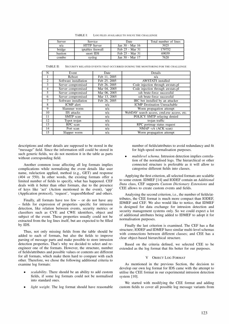
Server Service Date Total number of linesn/a HTTP Server Jan 30 - Mar 16 3925

bridge iptables firewall Feb 25 - Mar 31 179752bastion snort IDS Feb 25 - Mar 31 69039combo syslog Jan 30 - Mar 17 7620

TABLE I: LOG FILES AVAILABLE TO SOLVE THE CHALLENGE

N Event Date Details1 Reboot Feb 11, 2005 n/a2 Software installation Feb 25, 2005 AWSTATS installed3 Server compromised Feb 26, 2005 Code injection through awstats.pl4 Server compromised Mar 04, 2005 Code injection through awstats.pl5 Server compromised Mar 06, 2005 ssh brute-force successful6 Server compromised Mar 13, 2005 ssh brute-force successful7 Software installation Feb 26, 2005 IRC bot installed by an attacker8 ICMP alert n/a ICMP Destination Unreachable9 Slammer worm n/a Worm propagation attempt10 IIS attacks n/a WebDAV search access, cmd.exe access, etc.11 SMTP scan n/a POLICY SMTP relaying denied12 Typot trojan n/a trojan traffic13 RPC scan n/a RPC portmap status request14 Port scan n/a NMAP -sA (ACK scan)15 Slapper worm n/a Worm propagation attempt

TABLE II: SECURITY RELATED EVENTS THAT OCCURRED DURING THE MONITORING FOR THE CHALLENGE

descriptions and other details are supposed to be stored in the“message” field. Since the information still could be stored insuch generic fields, we do not mention it in the table as partswithout corresponding field.

Another common issue affecting all log formats impliescomplications while normalising the event details like username, rule/action applied, method (e.g., GET) and response(404 or 550). In other words, the existing formats offer alimited number of fields to specify, what has happened. CEFdeals with it better than other formats, due to the presenceof keys like ‘act’ (Action mentioned in the event), ‘app’(Application protocol), ‘request’, ‘requestMethod’ and others.

Finally, all formats have too few – or do not have any– fields for expression of properties specific for intrusiondetection, like relation between events, security metrics orclassifiers such as CVE and CWE identifiers, object andsubject of the event. These properties usually could not beextracted from the log lines itself, but are expected to be filledby IDS.

Thus, not only missing fields from the table should beadded to each of formats, but also the fields to improveparsing of message parts and make possible to store intrusiondetection properties. That’s why we decided to select and re-engineer one of the formats. However, the structure, numberof fields/attributes and possible values or contents are differentfor all formats, which make them hard to compare with eachother. Therefore, we chose the following additional criteria toexamine log formats:

• scalability. There should be an ability to add customfields, if some log formats could not be normalisedinto standard ones.

• light weight. The log format should have reasonable

number of fields/attributes to avoid redundancy and fitfor high-speed normalisation purposes.

• multilevel schema. Intrusion detection implies correla-tion of the normalised logs. The hierarchical or otherconnected structure is preferable as it will allow tocategorise different fields into classes.

Applying the first criterion, all selected formats are scalableto some extent. IDMEF [14] and IODEF contain an AdditionalData class, CEF supports Custom Dictionary Extensions andCEE allows to create custom events and fields.

Analysing the second criterion, i.e., the number of fields/at-tributes, the CEE format is much more compact than IODEF,IDMEF and CEF. We also would like to notice, that IDMEFis designed for data exchange for intrusion detection andsecurity management systems only. So we could expect a lotof additional attributes being added to IDMEF to adopt it fornormalisation purposes.

Finally the last criterion is examined. The CEF has a flatstructure; IODEF and IDMEF have similar multi-level schemaswith connections between different classes; and CEE has aclear object-based hierarchical structure.

Based on the criteria defined, we selected CEE to beextended as the log format that fits better for our purposes.

V OBJECT LOG FORMAT

As mentioned in the previous Section, the decision todevelop our own log format for IDS came with the attempt toutilise the CEE format in our experimental intrusion detectionsystem [10].

We started with modifying the CEE format and addingcustom fields to cover all possible log message variants from

123

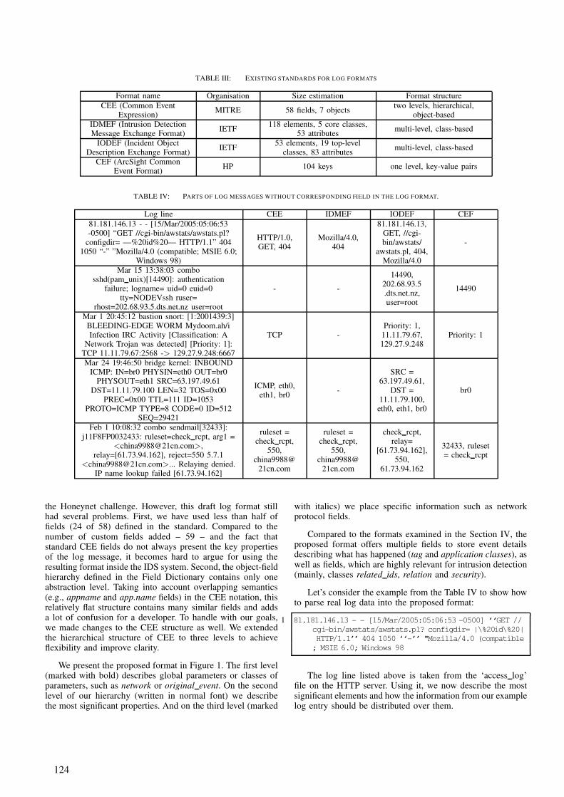
Format name Organisation Size estimation Format structureCEE (Common Event

Expression)MITRE 58 fields, 7 objects two levels, hierarchical,

object-basedIDMEF (Intrusion DetectionMessage Exchange Format) IETF

118 elements, 5 core classes,53 attributes multi-level, class-based

IODEF (Incident ObjectDescription Exchange Format)

IETF 53 elements, 19 top-levelclasses, 83 attributes

multi-level, class-based

CEF (ArcSight CommonEvent Format) HP 104 keys one level, key-value pairs

TABLE III: EXISTING STANDARDS FOR LOG FORMATS

Log line CEE IDMEF IODEF CEF81.181.146.13 - - [15/Mar/2005:05:06:53-0500] “GET //cgi-bin/awstats/awstats.pl?

configdir= —%20id%20— HTTP/1.1” 4041050 “-” ”Mozilla/4.0 (compatible; MSIE 6.0;

Windows 98)

HTTP/1.0,GET, 404

Mozilla/4.0,404

81.181.146.13,GET, //cgi-bin/awstats/

awstats.pl, 404,Mozilla/4.0

-

Mar 15 13:38:03 combosshd(pam unix)[14490]: authentication

failure; logname= uid=0 euid=0tty=NODEVssh ruser=

rhost=202.68.93.5.dts.net.nz user=root

- -

14490,202.68.93.5.dts.net.nz,user=root

14490

Mar 1 20:45:12 bastion snort: [1:2001439:3]BLEEDING-EDGE WORM Mydoom.ah/iInfection IRC Activity [Classification: A

Network Trojan was detected] [Priority: 1]:TCP 11.11.79.67:2568 -> 129.27.9.248:6667

TCP -Priority: 1,

11.11.79.67,129.27.9.248

Priority: 1

Mar 24 19:46:50 bridge kernel: INBOUNDICMP: IN=br0 PHYSIN=eth0 OUT=br0

PHYSOUT=eth1 SRC=63.197.49.61DST=11.11.79.100 LEN=32 TOS=0x00

PREC=0x00 TTL=111 ID=1053PROTO=ICMP TYPE=8 CODE=0 ID=512

SEQ=29421

ICMP, eth0,eth1, br0

-

SRC =63.197.49.61,

DST =11.11.79.100,eth0, eth1, br0

br0

Feb 1 10:08:32 combo sendmail[32433]:j11F8FP0032433: ruleset=check rcpt, arg1 =

<[email protected]>,relay=[61.73.94.162], reject=550 5.7.1

<[email protected]>... Relaying denied.IP name lookup failed [61.73.94.162]

ruleset =check rcpt,

550,china9988@

21cn.com

ruleset =check rcpt,

550,china9988@

21cn.com

check rcpt,relay=

[61.73.94.162],550,

61.73.94.162

32433, ruleset= check rcpt

TABLE IV: PARTS OF LOG MESSAGES WITHOUT CORRESPONDING FIELD IN THE LOG FORMAT.

the Honeynet challenge. However, this draft log format stillhad several problems. First, we have used less than half offields (24 of 58) defined in the standard. Compared to thenumber of custom fields added – 59 – and the fact thatstandard CEE fields do not always present the key propertiesof the log message, it becomes hard to argue for using theresulting format inside the IDS system. Second, the object-fieldhierarchy defined in the Field Dictionary contains only oneabstraction level. Taking into account overlapping semantics(e.g., appname and app.name fields) in the CEE notation, thisrelatively flat structure contains many similar fields and addsa lot of confusion for a developer. To handle with our goals,we made changes to the CEE structure as well. We extendedthe hierarchical structure of CEE to three levels to achieveflexibility and improve clarity.

We present the proposed format in Figure 1. The first level(marked with bold) describes global parameters or classes ofparameters, such as network or original event. On the secondlevel of our hierarchy (written in normal font) we describethe most significant properties. And on the third level (marked

with italics) we place specific information such as networkprotocol fields.

Compared to the formats examined in the Section IV, theproposed format offers multiple fields to store event detailsdescribing what has happened (tag and application classes), aswell as fields, which are highly relevant for intrusion detection(mainly, classes related ids, relation and security).

Let’s consider the example from the Table IV to show howto parse real log data into the proposed format:

1 81.181.146.13 - - [15/Mar/2005:05:06:53 -0500] ‘‘GET //cgi-bin/awstats/awstats.pl? configdir= |\%20id\%20|HTTP/1.1’’ 404 1050 ‘‘-’’ "Mozilla/4.0 (compatible; MSIE 6.0; Windows 98

The log line listed above is taken from the ‘access log’file on the HTTP server. Using it, we now describe the mostsignificant elements and how the information from our examplelog entry should be distributed over them.

124

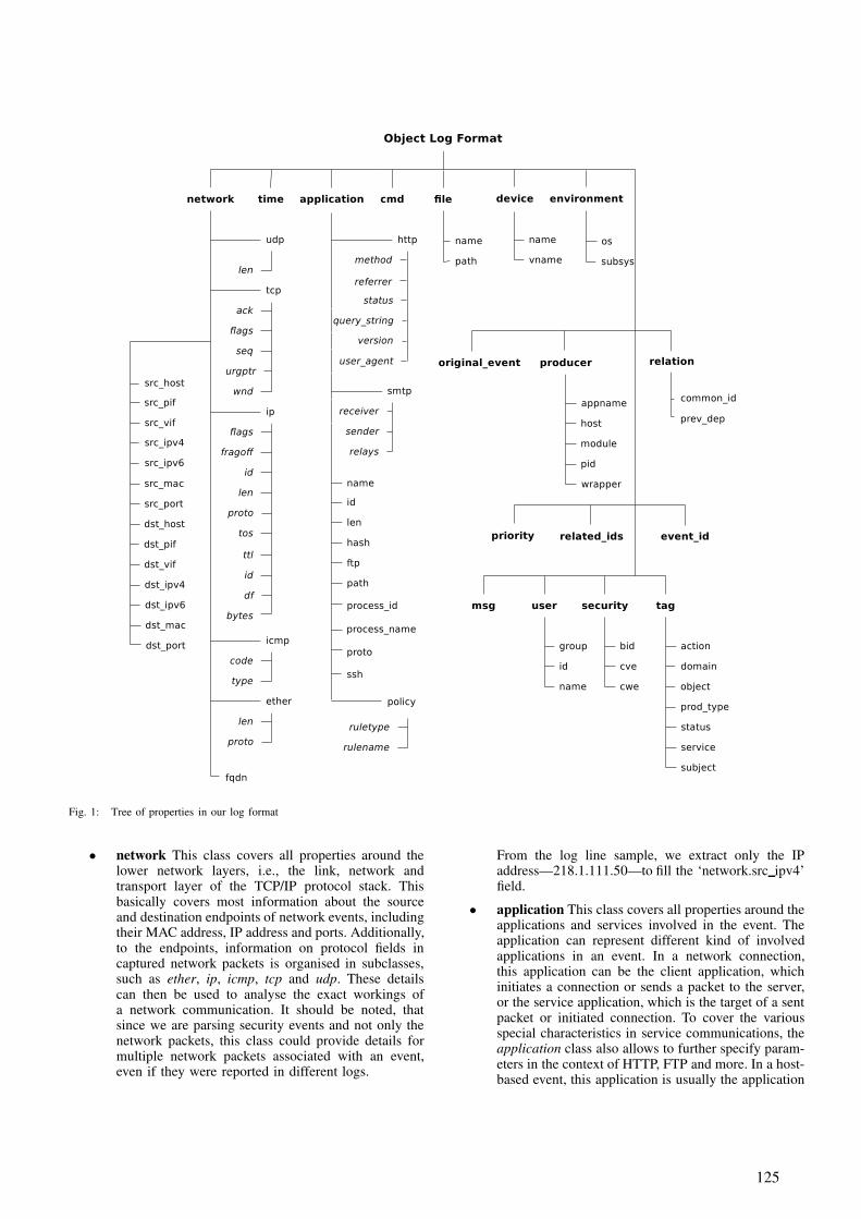
Fig. 1: Tree of properties in our log format

• network This class covers all properties around thelower network layers, i.e., the link, network andtransport layer of the TCP/IP protocol stack. Thisbasically covers most information about the sourceand destination endpoints of network events, includingtheir MAC address, IP address and ports. Additionally,to the endpoints, information on protocol fields incaptured network packets is organised in subclasses,such as ether, ip, icmp, tcp and udp. These detailscan then be used to analyse the exact workings ofa network communication. It should be noted, thatsince we are parsing security events and not only thenetwork packets, this class could provide details formultiple network packets associated with an event,even if they were reported in different logs.

From the log line sample, we extract only the IPaddress—218.1.111.50—to fill the ‘network.src ipv4’field.

• application This class covers all properties around theapplications and services involved in the event. Theapplication can represent different kind of involvedapplications in an event. In a network connection,this application can be the client application, whichinitiates a connection or sends a packet to the server,or the service application, which is the target of a sentpacket or initiated connection. To cover the variousspecial characteristics in service communications, theapplication class also allows to further specify param-eters in the context of HTTP, FTP and more. In a host-based event, this application is usually the application

125

that initiates an action, like an application that writes a file. T he semantics o f the s pecified application can be obtained from the subject and object field o f the tag class.Analysing the example log line, it is possible to notice, that the application is a user agent, so the ‘application.http.user agent’ field should be filled with “Mozilla/4.0 (compatible; MSIE 4.01; Windows 95)” line and ‘application.http.query string’ field – with the following line:“GET /scripts/..%c1%9c../winnt/system32/cmd.exe?/c+dir HTTP/1.0”.

• producer This class gives information on the applica-tion that observed and eventually persisted an event.It should describe the first application that persistedthe events and should not be changed to one of theintermediate processing applications.In our example, a producer is a HTTP server, namely“Apache HTTP Server”, which should be written intothe ‘producer.appname’. If we would know somedetails about the host from the other log lines, wecould also fill the ‘producer.host’ field, e.g., withhttp server.

• file This class describes the files that were involved inan event. A file can appear in different contexts, i.e.,mainly as a data source and target of access operations,such as read and write. In the case of an FTP or HTTPconnection, this parameter could give information onthe accessed resource. Similar to the application class,the concrete context for one event is defined by thesubject and object field of the tag class.Considering the sample log line, the ‘file.name’field will contain ‘cmd.exe’ and ‘file.path’ –/scripts/..%c1%9c../winnt/system32/cmd.exe’.

• original event This field keeps the original log asfound in the log source. This is usually a string of thelog line or the fields of that where found log database.The whole sample log line should be filled into the‘original event’ in our case.

• relation This class serves the cases when severalevents are related to each other. In the case of multipleevents sharing a common identifier for correlation,this identifier is stored in the common id field. Theprev dep property indicates if the current event de-pends on a previous one.For the example considered, these fields will be empty,because the log event is standalone and not related toany other events.

• tag This class provides abstract information on topof the message details, mainly to categorise and tagevents. As this information is not always directlyrepresented in the log data, this is required to be setby the user. In some cases the action (and other fieldsas well) cannot be explicitly identified with a singleterm. Therefore, we propose all fields within this classas multi-value.E.g., the ‘tag.action’ could be {get,access},‘tag.subject’ – host or user client, ‘tag.object’ –file or web document, ‘tag.prod type’ – web server

and ‘tag.service’ could be web.

• security This class provides links to identifier ofvulnerability, related to the logged event. For example,‘security.cve’ could be “CVE-2010-4369”.

• event id This field contains a unique internal id ofthe event. This should be unique among all generatedevents in a management system. For our example, weused an SQL database for automatic id generation.

The developed format structure is easy to present, ex-tend and map into database relations. These features sim-plify the developer’s tasks and clarify the semantics of fieldswith similar names. For example, now the former appnameand app.name fields are easier distinguishable by using pro-ducer.appname and application.name as names. Finally, with107 fields used, we were able to effectively normalise everylog message from the dataset. After the normalisation step,most of the attacks could be discovered using simple searchqueries, as shown in the next section.

VI THE ROLE OF THE COMMON LOG FORMAT IN ATTACKDETECTION

As mentioned earlier, we normalise files before searchingfor attacks. This pre-processing step includes parsing of thelogs into described log format with regular expressions andinserting them into the SQL database.

The proposed log format allows to detect attacks described in the Table II using simple queries, without the usage of a correlation engine or other advanced intrusion detection techniques. The challenge winners on the other part have used self-written scripts and manual analysis [15, 16]. We now provide several use cases to demonstrate the benefits o f the proposed log format. E.g., to check for SMTP scans, we use the following query:

1 select * from event where application_protocol = ’smtp’and tag_status = ’failure’

All 220 log lines returned correspond to event 11 fromTable II. These lines include both sendmail messages from themail server (“combo”) and snort alerts from the logging server(“bastion”).

Next, to detect the code injection attempts, we suggestanother simple SQL query:

1 SELECT * FROM event WHERE application_cmd LIKE ’% %\%3b%’ ESCAPE ’\’ AND application_protocol = ’http’ORDER BY time

We search for a semicolon in the URL being processedby any HTTP Server mentioned in the log files1. The resultcontains 20 logs, all of them related to the code injection casesthrough awstats.pl. 15 logs correspond to events 3 and 7 fromTable II, two other lines to event 4. The remaining 3 lineswere related to the awstats.pl code injection attempts on 2 and12 March 2005, not being mentioned in the official challengeresults2.

1In almost all cases, the semicolon in the URL indicates a malicious eventlike code injection.

2these events were found by the challenge winner [15].

126

HTTP requestheader element Log Format Object Patterns

HostNetwork.fqdn &

File.path

“eval(”, “concat”, “union!+!select”, “(null)”,“base64 ”, “/localhost”, “/pingserver”,“/config.”, “/wwwroot”, “/makefile”,“crossdomain.”, “proc/self/environ”,

“etc/passwd”, “.exe”, “.sql”, “.ini”, “/.bash”,“/.svn”, “/.tar”, “ ”, “¡”, “¿”, “/=”, “...”,

“+++”, “/&&”

Content-Location

Application. http.query string

“?”, “:”, “[”, “]”, “../”, “127.0.0.1”,“loopback”, “%0a”, “%0d”, “%22”, “%27”,“%3b”, “%3c”, “%3e”, “%00”, “%2e%2e”,

“%25”, “union”, “input file”, “execute”,“mosconfig”, “environ”, “scanner”, “path=.”,

“mod=.”

User-AgentApplication. http.

user agent

”binlar”, ”casper”, ”cmswor”, ”diavol”,”dotbot”, ”finder”, ”flicky”, ”jakarta”,

”libwww”, ”nutch”, ”planet”, ”purebot”,”pycurl”, ”skygrid”, ”sucker”, ”turnit”,

”vikspi”, ”zmeu”

TABLE V: HTTP PATTERNS.

Obviously, many attacks could not be captured with suchsimple queries. But the log format structure allows a developerto easily create more sophisticated checks. Please see Table Vfor sample patterns of malicious HTTP events. The proposedobject hierarchy of the log format allows specifying object-specific patterns (in this example – patterns for differentelements of HTTP request header). This flexibility simplifiescreation of rules for matching of malicious events. Now, ifwe check the normalised log messages with all the patternsselected, we could match 740 HTTP events related to line 10from Table II, as well as 35 redirects and 2 cases of calls tothe ‘libwww’ library.

VII DISCUSSION

We have shown how the common log format, if thoroughlydeveloped with the regard for specific usage conditions (intru-sion detection in our case), could facilitate a lot of operations,including search for attack patterns and correlation of eventsfrom different servers. However, the structure of existing logformat standards could differ from the one imposed by specificuse conditions. On the one hand, common log formats beingdeveloped nowadays (CEE [3] and IODEF [6]) try to handleall possible use cases. Such unified approach often needs amanual adoption to be a best fit for a specific use case. On thethe other hand, log formats, specially established for intrusiondetection sometimes have a limited scope. IDMEF [14] definesthe format for inter-communication only (between intrusiondetection, response and management systems). And CEF [5]has a flat hierarchy, which makes it less flexible in comparisonwith object-based log formats like CEE [3].

Within our proposed format we try to utilise the strongsides of both approaches and design the flexible object logformat that fits the specific purposes, but could be easilyextended for generic use cases. However, we do not intend tocreate a replacement for standards proposed by MITRE [17],IETF [18] and others. Rather, we hope that existed standardscould be more flexible to be used for specific purposes andbe able to combine extensible structure, light weight and mul-tifarious capabilities, such as search and correlation facilities

for intrusion detection systems.

REFERENCES

[1] D. Casey, “Turning log files into a security asset,” Network Security,vol. 2008, no. 2, pp. 4–7, 2008.

[2] L. Yang, P. Manadhata, W. Horne, P. Rao, and V. Ganapathy,“Fast submatch extraction using obdds,” in Proceedings of the eighth ACM/IEEE symposium on Architectures for networking and communications systems, ser. ANCS ’12. New York, NY, USA: ACM, 2012, pp. 163–174. [Online]. Available: http://doi.acm.org/10. 1145/2396556.2396594.

[3] “Common Event Expression White Paper,” June 2008.

[4] G. T. McGuire, “The state of security automation standards -2011,” http://www.mitre.org/work/tech papers/2011/11 3822/, Novem-ber 2011.

[5] ArcSight, “Common Event Format,” http://mita-tac.wikispaces.com/file/view/CEF+White+Paper+071709.pdf, July 2009.

[6] R. Danyliw, J. Meijer, and Y. Demchenko, “The incident object descrip-tion exchange format,” IETF RFC5070, December 2007.

[7] “BlackStratus LOG Storm,” http://www.blackstratus.com/enterprise/supported-technologies/log-storm/.

[8] “Sawmill log analysis tool,” http://www.sawmill.net/.

[9] “Open Source Host-based Intrusion Detection System,” http://www.ossec.net/.

[10] S. Roschke, F. Cheng, and C. Meinel, “An extensible andvirtualization-compatible ids management architecture,” in Proceedings of the 2009 Fifth International Conference on Information Assurance and Security - Volume 02, ser. IAS ’09. Washington, DC, USA: IEEE Computer Society, 2009, pp. 130–134. [Online]. Available: http://dx.doi.org/10.1109/IAS.2009.151.

[11] “HPI Vulnerability Database,” https://www.hpi-vdb.de/.

[12] “The Honeynet Project,” http://honeynet.org/.

[13] A. Chuvakin, “Scan 34 - analyze real honeynet logs for attacks andactivity,” http://old.honeynet.org/scans/scan34/, February 2005.

[14] H. Debar, D. Curry, and B. Feinstein, “The Intrusion Detection MessageExchange Format (IDMEF),” IETF RFC4765, March 2007.

[15] M. Richard, M. Ligh, A. Magnusson, S. Seale, and K. Standridge,“Project honeynet scan of the month 34,” http://old.honeynet.org/scans/scan34/sols/1/index.html, May 2005.

[16] C. Kronberg and A. Freeworld, “Analysis of the logfiles given inSotM34,” http://old.honeynet.org/scans/scan34/sols/2/proc.pdf, 2005.

[17] “The MITRE Corporation,” http://www.mitre.org/.

[18] “Internet Engineering Task Force,” http://www.ietf.org/.

127

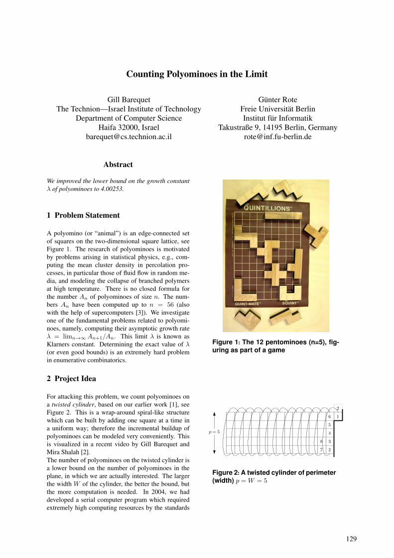
Counting Polyominoes in the Limit

Gill BarequetThe Technion—Israel Institute of Technology

Department of Computer ScienceHaifa 32000, Israel

[email protected]

Gunter RoteFreie Universitat BerlinInstitut fur Informatik

Takustraße 9, 14195 Berlin, [email protected]

Abstract

We improved the lower bound on the growth constantλ of polyominoes to 4.00253.

1 Problem Statement

A polyomino (or “animal”) is an edge-connected setof squares on the two-dimensional square lattice, seeFigure 1. The research of polyominoes is motivatedby problems arising in statistical physics, e.g., com-puting the mean cluster density in percolation pro-cesses, in particular those of fluid flow in random me-dia, and modeling the collapse of branched polymersat high temperature. There is no closed formula forthe number An of polyominoes of size n. The num-bers An have been computed up to n = 56 (alsowith the help of supercomputers [3]). We investigateone of the fundamental problems related to polyomi-noes, namely, computing their asymptotic growth rateλ = limn→∞An+1/An. This limit λ is known asKlarners constant. Determining the exact value of λ(or even good bounds) is an extremely hard problemin enumerative combinatorics.

2 Project Idea

For attacking this problem, we count polyominoes ona twisted cylinder, based on our earlier work [1], seeFigure 2. This is a wrap-around spiral-like structurewhich can be built by adding one square at a time ina uniform way; therefore the incremental buildup ofpolyominoes can be modeled very conveniently. Thisis visualized in a recent video by Gill Barequet andMira Shalah [2].The number of polyominoes on the twisted cylinder isa lower bound on the number of polyominoes in theplane, in which we are actually interested. The largerthe width W of the cylinder, the better the bound, butthe more computation is needed. In 2004, we haddeveloped a serial computer program which requiredextremely high computing resources by the standards

Figure 1: The 12 pentominoes (n=5), fig-uring as part of a game

p = 5

1

3

4

5

6

7

8

2

2

Figure 2: A twisted cylinder of perimeter (width) p = W = 5

129

Figure 3: A Motzkin path

of that time, both in terms of running time and mainmemory, going up to width W = 22 with 32 GiBytesof main memory. Before the start of this project, thebounds on Klarner’s constant were 3.985 from belowand 4.6 from above. The bound 3.985 comes from thetwisted cylinder of width W = 23. We set out to pushthe lower bound above 4.


We used a Hewlett Packard DL980 G7 computer. Ithas 8 processors nodes with a total of 128 cores, and2048 GiB RAM in total. Each node is an Intel XeonX7560 Processor (8C, 2.26 GHz) with 24 MB cache,Intel64 architecture. Hyperthreading is used to allow16 processes to run on 8 “physical cores”, sharing cer-tain resources.

4 Findings

The basic program is an iteration which computes aseries of vectors y.Each iteration constructs a new iterate vector ynew

from the previous iterate yold in a simple loop:

for s := 1, . . . ,M :(∗) ynew[s] := ynew[succ0[s]] + yold[succ1[s]];

The pointer succ0[s] may be null, and in this case thecorresponding entry is not used.The vectors are indexed from 1 to M . Each entry rep-resents a state, which corresponds to some combina-torial information about a partially built polyomino.Successor states correspond to adding an occupied(succ1) or a free (succ0) cell. States are encoded byso-called Motzkin paths, paths in the directed acyclicnetwork shown in Figure 3, and these paths can be bi-jectively mapped to numbers between 1 and M . (Thenumber M of Motzkin paths is called a Motzkin num-ber.)In the iteration (∗), the vector ynew depends on it-self, but this is not a problem because succ0[s], if itis non-null, is always less than s. In fact, the statescan be partitioned into groups G0, G1, . . . , GW suchthat succ0[s] of an entry s ∈ Gi, if it is non-null,belongs to Gi+1. Thus, all entries s in a group Gi

can be treated in parallel, in a straightforward man-ner. The groups are processed sequentially in the orderGW , GW−1, . . . , G1, G0.The pointer arrays succ0[] and succ1[] are computedbeforehand.We first parallelized the existing program for using128 parallel processor cores. The programs are writ-ten in C, and we used the OpenMP compiler directivesfor parallelization. We handled the distribution of theloops over the processors explicitly.By May 1, 2013, we succeeded to run the iterationfor W = 26 in 3 hours using about 1 TeraByte ofmain memory, establishing a new record lower boundof 3.9989. The number of states for this case is M =73.007,772.801.Getting to W = 27 and thus pushing the lower boundon λ above 4.0 was only possible by engineering tricksthat saved memory at the expense of run-time, sinceotherwise the memory requirement would increase bya factor of 3 with each increase of W , and we have“only” 2 TeraBytes available.We used the following measures.

1. Eliminating a certain fraction of “unreachablestates” (about 11%). These states don’t contributeto the limit. Elimination of these states requireda change in the mapping between “reachable”Motzkin paths and integers.

2. “Bit-streaming” of the succ-arrays instead of stor-ing them in fixed 4-byte or 8-byte words. (Thesearrays are accessed only sequentially.)

3. Storing only one iterate vector instead of two forgroups G2, G3, . . ..

4. Complete elimination of the succ0-arrays; in-stead, these pointers are recomputed each timethey are needed. This required a streamlined pro-gram to accelerate the successor computation.

5. Streamlining the conversion between Motzkinpaths and integers, using precomputed and storedtables. We took care that each processor has ac-cess to its own copy of the table, and the table issmall enough to fit in the level-1 cache.

6. Writing checkpoints of intermediate results todisk.

On May 20, we succeeded to run the iteration forW = 27, using about 36 hours of runtime in total,distributed over several runs and writing intermediateresults to disk. The lower bound on λ broke throughthe mythical barrier of 4.0 after 120 iterations. After290 iterations, the lower bound converged to 4.00254,establishing the current record.With hindsight, it would not have been necessary towrite and read checkpoints to disk; on the other hand,it was good to have the data on disk for running anindependent check.

130

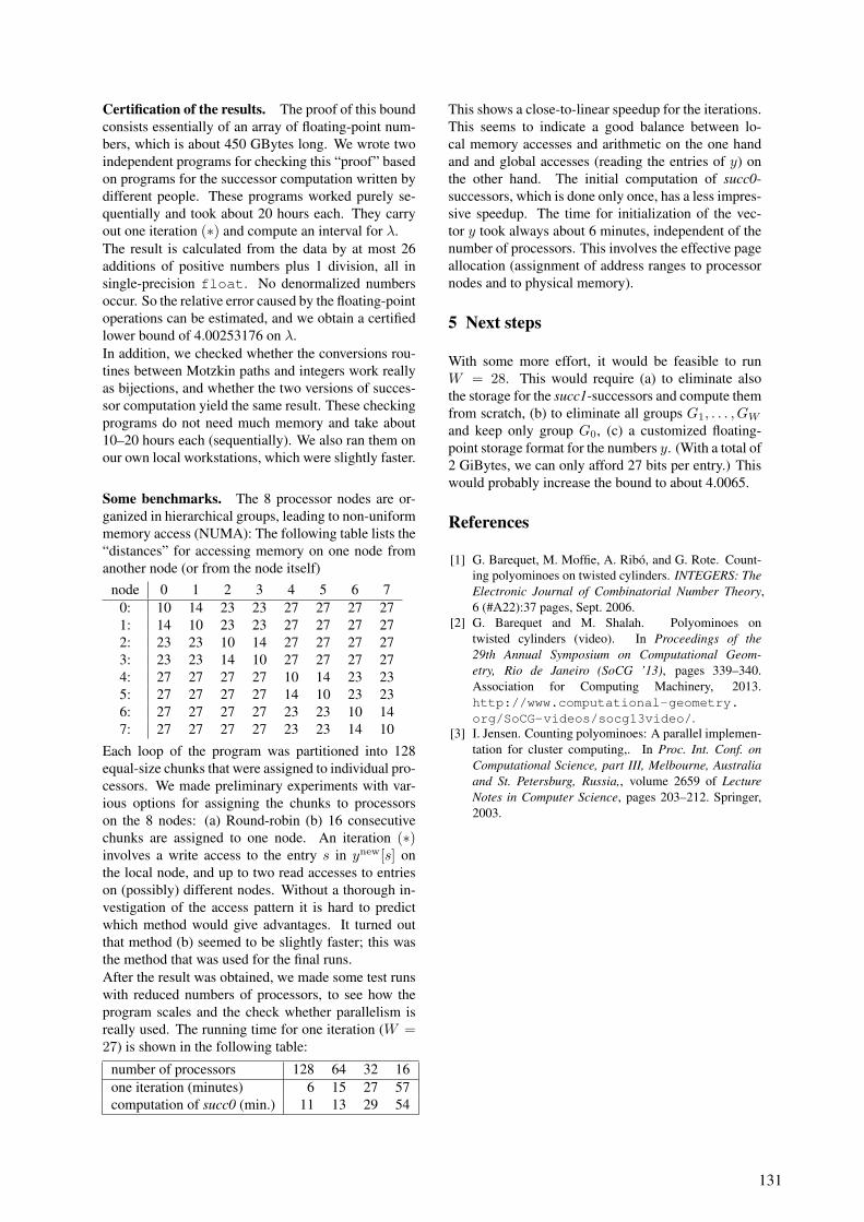
Certification of the results. The proof of this boundconsists essentially of an array of floating-point num-bers, which is about 450 GBytes long. We wrote twoindependent programs for checking this “proof” basedon programs for the successor computation written bydifferent people. These programs worked purely se-quentially and took about 20 hours each. They carryout one iteration (∗) and compute an interval for λ.The result is calculated from the data by at most 26additions of positive numbers plus 1 division, all insingle-precision float. No denormalized numbersoccur. So the relative error caused by the floating-pointoperations can be estimated, and we obtain a certifiedlower bound of 4.00253176 on λ.In addition, we checked whether the conversions rou-tines between Motzkin paths and integers work reallyas bijections, and whether the two versions of succes-sor computation yield the same result. These checkingprograms do not need much memory and take about10–20 hours each (sequentially). We also ran them onour own local workstations, which were slightly faster.

Some benchmarks. The 8 processor nodes are or-ganized in hierarchical groups, leading to non-uniformmemory access (NUMA): The following table lists the“distances” for accessing memory on one node fromanother node (or from the node itself)

node 0 1 2 3 4 5 6 70: 10 14 23 23 27 27 27 271: 14 10 23 23 27 27 27 272: 23 23 10 14 27 27 27 273: 23 23 14 10 27 27 27 274: 27 27 27 27 10 14 23 235: 27 27 27 27 14 10 23 236: 27 27 27 27 23 23 10 147: 27 27 27 27 23 23 14 10

Each loop of the program was partitioned into 128equal-size chunks that were assigned to individual pro-cessors. We made preliminary experiments with var-ious options for assigning the chunks to processorson the 8 nodes: (a) Round-robin (b) 16 consecutivechunks are assigned to one node. An iteration (∗)involves a write access to the entry s in ynew[s] onthe local node, and up to two read accesses to entrieson (possibly) different nodes. Without a thorough in-vestigation of the access pattern it is hard to predictwhich method would give advantages. It turned outthat method (b) seemed to be slightly faster; this wasthe method that was used for the final runs.After the result was obtained, we made some test runswith reduced numbers of processors, to see how theprogram scales and the check whether parallelism isreally used. The running time for one iteration (W =27) is shown in the following table:

number of processors 128 64 32 16one iteration (minutes) 6 15 27 57computation of succ0 (min.) 11 13 29 54

This shows a close-to-linear speedup for the iterations.This seems to indicate a good balance between lo-cal memory accesses and arithmetic on the one handand and global accesses (reading the entries of y) onthe other hand. The initial computation of succ0-successors, which is done only once, has a less impres-sive speedup. The time for initialization of the vec-tor y took always about 6 minutes, independent of thenumber of processors. This involves the effective pageallocation (assignment of address ranges to processornodes and to physical memory).

5 Next steps

With some more effort, it would be feasible to runW = 28. This would require (a) to eliminate alsothe storage for the succ1-successors and compute themfrom scratch, (b) to eliminate all groups G1, . . . , GW

and keep only group G0, (c) a customized floating-point storage format for the numbers y. (With a total of2 GiBytes, we can only afford 27 bits per entry.) Thiswould probably increase the bound to about 4.0065.

References

[1] G. Barequet, M. Moffie, A. Ribo, and G. Rote. Count-ing polyominoes on twisted cylinders. INTEGERS: The Electronic Journal of Combinatorial Number Theory, 6 (#A22):37 pages, Sept. 2006.

[2] G. Barequet and M. Shalah. Polyominoes ontwisted cylinders (video). In Proceedings of the29th Annual Symposium on Computational Geom-etry, Rio de Janeiro (SoCG ’13), pages 339–340.Association for Computing Machinery, 2013.http://www.computational-geometry.org/SoCG-videos/socg13video/.

[3] I. Jensen. Counting polyominoes: A parallel implemen-tation for cluster computing,. In Proc. Int. Conf. onComputational Science, part III, Melbourne, Australiaand St. Petersburg, Russia,, volume 2659 of LectureNotes in Computer Science, pages 203–212. Springer,2003.

131

Evaluation of Visual Concept Classifiers

Peter RetzlaffHasso-Plattner-Institut


[email protected]

Christian HentschelHasso-Plattner-Institut


[email protected]

Harald SackHasso-Plattner-Institut

Prof.-Dr.-Helmert-Str. 2-3 14482 Potsdam

[email protected]

Abstract

Visual Concept Detection aims to classify imagesbased on their content. Bag-of-(Visual-)Words fea-tures that quantize and count local gradient distri-butions in images similar to counting words in textshave proven to be meaningful image representations.In combination with supervised machine learning ap-proaches such as AdaBoost, models for nearly everyvisual content can be learned by sufficient labeledtraining data. Similar to text classification the clas-sification of an image depends on a weighted combi-nation of the visual words from the vocabulary and theclassifier is expected to learn these weights in order toobtain best results. Hence, the learned weights or im-portances of each visual word are a strong indicatorfor the robustness and reasonableness of the overallconcept model. This work visualizes learned conceptmodels by colorizing the image pixels using the impor-tance value of the corresponding local visual word us-ing a heatmap-like representation. Thereby we explic-itly show sources of misclassification and thus help tounderstand and improve varying results for differentconcept classes. Due to the high-dimensional natureof the employed features training the concept modelsis an expensive process when regarding both – mem-ory and computational resources. Multi-core architec-tures can help to significantly reduce the time requiredto train a model for a given visual concept and avail-ability of large main memory guarantees that trainingcan be preformed without latency due to disk I/O.

1 Introduction

Given a set of images and a set of concepts, the task ofvisual concept classification is to assign one or more

of the concepts to each of the images. The conceptsmay describe the image contents, like ’car’, ’person’or ’landscape’, as well as more abstract characteristics,e.g. whether it is over- or underexposed. This task iscommonly solved by describing the images as vectorsof local and global features, such as color and gradienthistograms. Supervised machine learning techniquesare subsequently used to learn how to separate positivefrom negative examples of each concept class.

One approach that is commonly used to representimages is the Bag-of-(Visual-)Words model (BoW),which extends an idea from text retrieval to visual clas-sification [3, 8]. In text classification systems, eachtext can be represented by a histogram of the frequen-cies of each possible word from a given vocabulary.That is, a text is characterized by the number of oc-currences of each possible word, independently of theword order. Similarly, we describe an image as a fre-quency distribution of visual words. While the notionof a word in natural languages is clear, visual wordsare less easy to describe. Typically local image char-acteristics are used to represent visual words such asintensity changes, i.e. the gradients in an image re-gion.

By representing images as histograms of visual words,they are mapped into a high dimensional vector space.Classification of images can then be considered as asupervised learning problem trying to separate vectorscorresponding to positive from those correspondingto negative example images of a given concept class.Each vector dimension represents a specific visualword and gaining insight into the influence of each di-mension to the overall classification result may enableus to gain an understanding of the concept model, thatis learned. Thereby, sources of misclassification canbe better explained and, finally, classification resultsmay be improved by using these insights.

133

Therefore, the goal of this project is to evaluate meansto visualize the influence of visual words on the overallclassification result, in terms of a heatmap. This canbe achieved by first evaluating the importance of eachfeature to the trained concept model and then assigningto each pixel of the image an importance value basedon the visual words it contributes to.This paper is structured as follows: In Section 2 wegive some background on supervised machine learningin general and ensemble methods in particular that areused within this work to learn a concept model. Next,we present implementation details of the proposed ap-proach in Section 3 and show where and how FutureSOC Lab resources were used in order to increase thetraining performance. Section 4 provides a short anal-ysis of our results and finally Section 5 summarizesthe paper and gives a brief outlook of the work we areplanning to do in the future.

2 Visual Concept Modeling

As discussed in the introduction, we perform visualconcept classification by applying supervised machinelearning techniques to Bag-of-Visual-Words featurevectors. In this section we therefore briefly introduceBag-of-Visual-Words feature extraction and describethe machine learning approach chosen to train a visualconcept model. Different from standard approachesfor Bag-of-Visual-Words classification [3, 8] we donot use kernel-based Support Vector Machines sincethese do not allow for deriving feature relevance froma learned concept model.

2.1 Bag of Visual Words Extraction

Following [3, 8] we use local histograms of gradientsto describe local properties of images that form a vi-sual word space. The Scale-Invariant Feature Trans-form (SIFT, [5]) is the most widely used local gra-dient descriptor for Bag-of-Visual-Words representa-tions. SIFT computes orientation invariant histogramsof gradients at selected regions of interest (i.e. key-points) in an image. While this approach is especiallyuseful when matching image regions, in image clas-sification one usually strives for a holistic image rep-resentation and therefore computes SIFT descriptorsat densely sampled keypoints. We quantize local fea-tures by clustering a random subset of SIFT vectors ex-tracted from the training image using k-means cluster-ing. The derived centroids form our vocabulary, whichis fixed to a size of k = 4000 visual words, a com-mon size in related research. Finally, for each imagea nearest neighbor search is performed to assign eachkeypoint’s SIFT-descriptor to the most similar visualword in the vocabulary. The frequency distributionsof the visual words within an image is represented asa histogram consisting of k bins, one for each visualword. This histogram is then normalized forming a

vector of k real numbers, which represents the givenimage.

2.2 Supervised machine learning

Given the set of possible instances X , the set ofpossible labels Y and a set of labeled examples{(x1, y1), .., (xn, yn)} with xi ∈ X and yi ∈ Y , thetask of supervised machine learning is to infer a func-tion h : X → Y , that correctly maps the xi to yi. Thefunction h maps from the space of all possible inputsX to a finite set of outputs Y and is often called thehypothesis of the machine learning algorithm.For the task at hand, the elements of X would be ab-stract representations of the given images such as Bag-of-Visual-Words representation and the elements of Ycorrespond to the concept labels (e.g. ’landscape’),which shall be learned. Typically in image classifi-cation, the problem of detecting |Y | different conceptsis treated as a binary classification problem where thetask is to separate images into two groups on the basisof whether they depict a specific concept or not.For a set of labeled examples

S = {(x1, y1), .., (xn, yn)}

and a hypothesis h we define the (training) error rateεh of h to be

εh =1

|S|·

|S|∑i=1

I(h(xi) 6= yi)

where I(·) is the indicator function. That is, the errorrate of hypothesis h is the fraction of samples, that areincorrectly labeled by h.We distinguish between weak and strong learning al-gorithms. A strong learning algorithm is one, thatcan achieve an arbitrarily low error rate with arbitrar-ily high probability, given sufficient time and trainingsamples. In contrast, weak learning algorithms areonly required to perform better than random guessing.That is, their error rate has to be smaller than 0.5 incase of a binary classification task.

2.3 Boosting and bagging algorithms

Schapire [7] proved that it is possible to combine mul-tiple weak learners into a single strong learner. That is,given a sufficient number of learning algorithms, thatperform only slightly better than a random guess, wecan create an algorithm that predicts the data with anarbitrarily small error rate.This finding justifies the use of a number of learningalgorithms known as ensemble methods. Ensemblemethods try to achieve high predictive performance bycombining multiple learners, that are diversified eitherby training them on different (random) subsets of data(bootstrap aggregating or bagging, see [1]) or by iter-atively building models that emphasize samples which

134

where mis-classified by previous models (boosting,see [7]). Two prominent examples of each of theseclasses of algorithms are AdaBoost [4] by Freund andShapire and Random Forests [2].AdaBoost is an iterative algorithm, which iterates overtraining a weak learner using the set of (weighted)training examples {(x1, y1)...(xn, yn)}. It is commonto choose the sample weights {w1, .., wn} to be uni-formly distributed for the first iteration. After each it-eration the weights are updated proportionally to theerror rate of the current weak learner, assigning largerweights to samples, which have previously been misla-beled. Thus, intuitively speaking, samples with higherweights are more ’difficult’ to classify than others andthe weak learner is forced to ’concentrate’ more onclassifying them correctly. After a defined numberof iterations T , the algorithm stops and outputs its fi-nal hypothesis, which corresponds to a weighted sumof all the weak learner’s predictions. Obviously thechoice of the weak learning algorithm has some im-pact on the outcome of AdaBoost. Typically decisionstumps1 are used, as they are very easy to implementand efficiently computable.Another well known algorithm that combines manysimple decision trees into a strong learning algorithmis the Random Forest algorithm. It trains each weaklearner on a randomly selected subset of the trainingdata and at each node chooses a random subsampleof the features to determine the decision for that nodefrom. For the classification task, the final output ofa Random Forest is the mode2 of the outputs of all itstrees. The weak learners in the case of Random Forestsare full-grown decision trees.While decision stumps as well as decision trees pro-vide ad hoc methods for computing individual fea-ture importance, they lack enough expressiveness tocorrectly represent complex problems such as visualconcept modeling. However, following [7], we useAdaBoost and Random Forests that allow for com-plex problem space representations as well as for fea-ture importance estimation simply by computing theweighted sum of importances of the individual weaklearners. This makes boosting and bagging algorithmsan ideal choice for this project, as they achieve betterclassification performance than the underlying, sim-pler algorithms, while still allowing us to easily as-sess the importance of single Bag-of-Visual-Wordsfeatures for classification.The computation of an individual weak learner is typ-ically quite fast. However, we need to train severalthousand weak learners for each AdaBoost classifier.Though the run-time scales linearly with the number ofweak learners, one training session may need severalhours to complete. Considering the fact, that we needto train classifiers for many different parameter combi-nations (see Section 3.2) and as many different concept

1decision trees with only one or very few decision nodes2the classification value, that appears most often

classes as possible, this project would soon become in-feasible without utilization of the Future SOC’s paral-lel architecture.Bagging methods such as Random Forests provide astraightforward parallelization strategy, as all the weaklearners operate completely independent from eachother on different subsets of the data. With boost-ing algorithms, in particular AdaBoost, it is not thatsimple, as this is an inherently iterative algorithm andeach iteration depends on the preceding one. Never-theless, we can still benefit greatly from parallel ar-chitectures simply by optimizing different parametersof AdaBoost concurrently through parallel grid search(see Section 3.2).

3 Implementation and Future SOC Labresources

This section describes the implementation aspects ofour approach focusing on the exploitation of the Fu-ture SOC SMP multicore architecture. We used a ma-chine equipped with 24 processor cores and 64 GB ofmain memory. Development and testing was done ona local machine and the Future SOC was used to per-form computational expensive and long-running taskson the complete dataset. This includes feature extrac-tion, training and grid search, and visualization. All ofthese tasks were parallelized and benefit largely froma multi-core architecture.For training and testing purposes we use the publiclyavailable ImageCLEF 2011 dataset for visual conceptclassification [6], which contains 8.000 training sam-ples, each manually labeled with a subset of 99 im-age categories. We evaluate our classifier on a set of10.000 images, also provided by ImageCLEF.

3.1 Feature Extraction

The feature extraction process includes several expen-sive computations, namely the computation of manySIFT descriptors, the clustering of a large number ofhigh-dimensional vectors and nearest-neighbor searchin their vector space. Therefore, in order to increasethe performance of Bag-of-Visual-Words extraction,each step of the process runs concurrently, making useof the available Future SOC multicore node. Extrac-tion of SIFT features on the 18.000 training and testingimages took approximately 1 hour compared to onefull day when computed on a single core (linear scal-ing is assumed here, since images are scaled to equalsize and thus the number of SIFT features extractedper image is the same). Generating the prototypes ofvisual words using k-means clustering can also be par-allelized since it consists of mainly independent dis-tance computations between training vectors. In ourimplementation clustering runs for 1 hour compared toan approximate 3-4 weeks of a respective serial imple-mentation. Finally, nearest-neighbor search for com-

135

puting the Bag-of-Visual-Words histograms of eachimage can be parallelized over all images and there-fore again provides a linear speed-up of factor 24 (1hour compared to 24 hours).

3.2 Concept Training and Grid Search

In our first implementation we focused on training ofconcept models using AdaBoost. There are a numberof parameters that influence the performance of Ada-Boost, namely the number of iterations T , the maxi-mum depth of each decision stump and the optimiza-tion criterion of the decision stumps. It is good prac-tice to optimize these parameters by performing a gridsearch and by using n−fold cross validation. We se-lected reasonable parameter ranges for each parameterand created a parameter grid by generating all possiblecombinations of the respective values. The training setis split into 3 stratified subsets where 2 folds are usedfor training the AdaBoost strong learner and the re-maining fold is used to test the derived hypothesis. Byiterating over all possible folds, we make sure to usethe whole training set as training data while avoidingtesting on training data at the same time (3-fold crossvalidation).We used extensive grid search to find a parameter com-bination that shows best results on the training set.While AdaBoost itself is hard to parallelize, we uti-lized the Future SOC’s parallel architecture to evaluateas many parameter combinations in parallel as possi-ble. As the models for each parameter combinationcan be learned independently of each other, this greatlyreduces the time needed for grid search and thus en-abled us to explore a much larger space of combina-tions in the given time. Hence, grid search was par-allelized by delegating the training for each parame-ter combination to a dedicated core. This lead to anAdaBoost classifier, that shows promising results of73.56% average precision on the test set for one of theconcepts (’landscape’).

3.3 Visualization

In order to visualize the impact of the various visualwords on the classification result, the importance ofeach feature for the obtained AdaBoost model needsto be computed. This is done by computing the impor-tance of the feature for each weak learner, which cor-responds to the information gain that is achieved whenthis feature is used in a decision node. These weakimportance values are then weighted by their corre-sponding weak learner’s weight and added together toget the feature importance for the overall AdaBoostclassifier. Each feature in a visual word vector cor-responds to a visual word in the aforementioned vo-cabulary. Hence, since each local SIFT vector in animage is directly mapped to the most similar visualword we can directly relate the visual word importance

to all corresponding SIFT vectors and thus to the re-spective keypoints where these features have been ex-tracted. By assigning each keypoint in an image theimportance value of its corresponding visual word wecreate an importance map of all pixels in the image forthe overall classification result depending on the com-puted concept model. This is done by setting the im-portance of a single pixel to be the weighted sum of theimportances of all keypoints which are near that pixel.The rationale for this approach is that visual wordswere formed by computing SIFT descriptors aroundkeypoints and therefore using pixel information in anarea around that keypoint. Therefore, each pixel in thatarea has some kind of influence on the resulting visualword and thus on its importance for classification. AsSIFT weighs the influence of pixel information on thefinal descriptor by applying a Gaussian, so do we to re-duce the importance of pixels with increasing distanceto their corresponding keypoints. We visualize the im-portance map by rendering a heatmap (see Fig. 1).

Again, we rely on the Future SOC parallel architectureto reduce the time needed for this process, as multipleimages can be processed in parallel. For the compu-tation of the heatmaps a near-linear speed-up can beachieved. However, disk I/O represents a bottleneckfor the parallelization of this stage, as the resulting im-ages need to be written to disk.

4 Results

At the time of this writing, we extracted Bag-of-Visual-Words features for the complete ImageCLEFdataset. We trained, evaluated and visualized an Ada-Boost classifier for the image concept ’landscape’,which is a scene related concept meaning that the im-portant features will most likely be spread over the im-age plane as a whole. Some of the resulting images canbe seen in Fig. 1.

The visualization shows no obvious pattern in exam-ples that were classified as positives, although occa-sionally an emphasis on horizontal edges can be seen,which may indicate that the horizon line is an impor-tant indicator for images depicting landscapes. Thisfinding is consistent with our initial assumption. How-ever, on many negatively classified images, large areasof homogeneous and very important features can beseen (see Fig. 1(d)). This seems to imply that thoselarge image regions have high discriminative value inthe sense that the existence of such a region is an indi-cator for a ’non-landscape’.

This result suggests, that the learned model is less ofa representation of what is typical for landscapes andmore a characterization of everything that is not. How-ever, a more thorough analysis of this and other con-cepts is needed to verify this assumption.

136

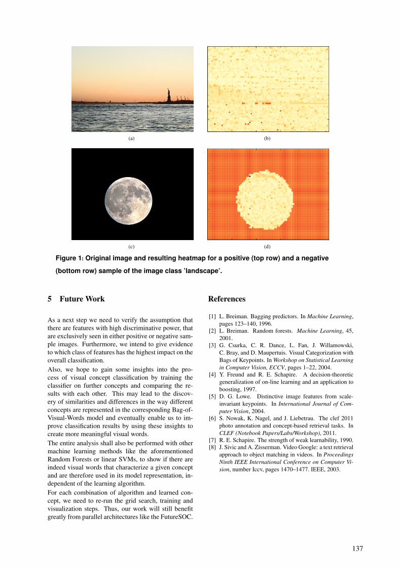
(a) (b)

(c) (d)

Figure 1: Original image and resulting heatmap for a positive (top row) and a negative

(bottom row) sample of the image class ’landscape’.

5 Future Work

As a next step we need to verify the assumption thatthere are features with high discriminative power, thatare exclusively seen in either positive or negative sam-ple images. Furthermore, we intend to give evidenceto which class of features has the highest impact on theoverall classification.Also, we hope to gain some insights into the pro-cess of visual concept classification by training theclassifier on further concepts and comparing the re-sults with each other. This may lead to the discov-ery of similarities and differences in the way differentconcepts are represented in the corresponding Bag-of-Visual-Words model and eventually enable us to im-prove classification results by using these insights tocreate more meaningful visual words.The entire analysis shall also be performed with othermachine learning methods like the aforementionedRandom Forests or linear SVMs, to show if there areindeed visual words that characterize a given conceptand are therefore used in its model representation, in-dependent of the learning algorithm.For each combination of algorithm and learned con-cept, we need to re-run the grid search, training andvisualization steps. Thus, our work will still benefitgreatly from parallel architectures like the FutureSOC.

References

[1] L. Breiman. Bagging predictors. In Machine Learning,pages 123–140, 1996.

[2] L. Breiman. Random forests. Machine Learning, 45,2001.

[3] G. Csurka, C. R. Dance, L. Fan, J. Willamowski,C. Bray, and D. Maupertuis. Visual Categorization withBags of Keypoints. In Workshop on Statistical Learningin Computer Vision, ECCV, pages 1–22, 2004.

[4] Y. Freund and R. E. Schapire. A decision-theoreticgeneralization of on-line learning and an application toboosting, 1997.

[5] D. G. Lowe. Distinctive image features from scale-invariant keypoints. In International Journal of Com-puter Vision, 2004.

[6] S. Nowak, K. Nagel, and J. Liebetrau. The clef 2011photo annotation and concept-based retrieval tasks. InCLEF (Notebook Papers/Labs/Workshop), 2011.

[7] R. E. Schapire. The strength of weak learnability, 1990.[8] J. Sivic and A. Zisserman. Video Google: a text retrieval

approach to object matching in videos. In ProceedingsNinth IEEE International Conference on Computer Vi-sion, number Iccv, pages 1470–1477. IEEE, 2003.

137

Landscape Virtualization Management tools at the HPI Future SOC Lab

Rami Akkad, Andre Deienno Pansani, Felix SalfnerSAP Innovation Center


{rami.akkad, andre.pansani, felix.salfner}@sap.com

Abstract

On-Demand services can only be provided in a prof-itable way if they are operated at minimum cost.Therefore, automated monitoring and task manage-ment are indispensable. Today, On-Demand provider-s use custom-made monitoring and management so-lutions. It is the goal of this project to assess theSAP LVM and HP Converged Cloud maintenance tool-s used at the FutureSOC Lab. We provide a classifi-cation of functionality (e.g. mass operations, report-ing, monitoring, provisioning of services) supportedby practical experiences from managing Future SOCLab resources with up to 16 SAP HANA instances, a1000 core cluster, storage solutions, etc.

1 Introduction

The ”HPI Future SOC Lab” is a cooperation of theHasso-Plattner-Institut (HPI) and industrial partners.Its mission is to enable and promote exchange and in-teraction between the research community and the in-dustrial partners. The HPI Future SOC Lab providesresearchers with free of charge access to a completeinfrastructure of state of the art hard- and software.This infrastructure includes components, which mightbe too expensive for an ordinary research environmen-t, such as servers with up to 64 cores and a 1000 corecluster. The offerings address researchers particularlyfrom but not limited to the areas of computer scienceand business information systems. Main areas of re-search include cloud computing, parallelization, andIn-Memory technologies.

In total 131 projects from 34 institutes were conductedusing the HPI FSOC Lab infrastructure since its launchin 2010.

Given the diverse and huge infrastructure the FutureSOC Lab comprises of, automated monitoring andtask management are indispensable to plan ahead andreduce costs.

2 Used Resources

SAP LVM is a management tool that enables the S-AP basis administrator to automate SAP system oper-ations including end-to-end SAP system copy/refreshoperations. The HP Converged Cloud powered byOpenstack [6] offers a portfolio of comprehensivecloud solutions to build, operate, and consume IT ser-vices that are open and enterprise-class across private,managed, and public clouds.We compared SAP NetWeaver Landscape Virtual-ization Management (SAP LVM) Enterprise Editionversion 2.0 and the HP Converged Cloud with HPCloudSystem Matrix version 7.2 Update 1. We clas-sified functionalities within both maintenance toolsbased on white papers and other information provid-ed by SAP and HP, and on experiences running thosetools inside the Future SOC Lab infrastructure.Furthermore we compared CPU load and memory uti-lization monitoring of both tools.

3 Feature Comparison and Assessment

We compared three categories which are

1. supported virtualization providers,

2. supported storage systems and

3. operations automation.

3.1 Supported virtualization providers

We compared SAP LVM and HP Converged Cloud re-garding their support of virtualization technologies ofthe following providers: Microsoft Hyper-V, VMware,KVM, Amazon, IBM and Novell.Both SAP LVM as well as HP Converged Cloud sup-port VMware vCenter (LVM VIM API 2.5 onwards)[3, 4]. Only HP Converged Cloud supports MicrosoftHyper-V [3, 4] and the KVM API [3, 4]. However, on-ly SAP LVM supports the Amazon AWS API [4], IB-M Hardware Management Console (for Power - HM-C V7R3.5.0 and for System z - HMC 2.10.1), IBM

139

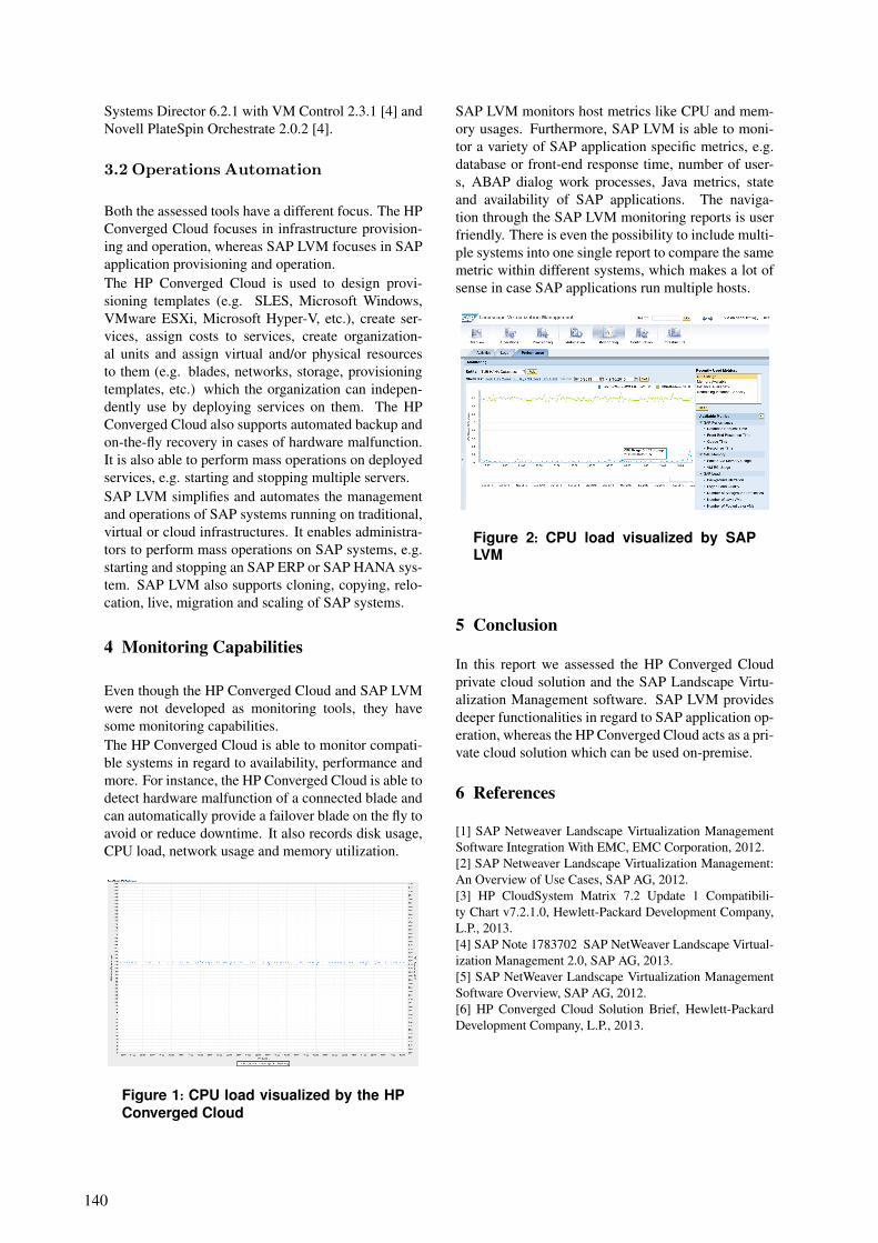
Systems Director 6.2.1 with VM Control 2.3.1 [4] andNovell PlateSpin Orchestrate 2.0.2 [4].

3.2 Operations Automation

Both the assessed tools have a different focus. The HPConverged Cloud focuses in infrastructure provision-ing and operation, whereas SAP LVM focuses in SAPapplication provisioning and operation.The HP Converged Cloud is used to design provi-sioning templates (e.g. SLES, Microsoft Windows,VMware ESXi, Microsoft Hyper-V, etc.), create ser-vices, assign costs to services, create organization-al units and assign virtual and/or physical resourcesto them (e.g. blades, networks, storage, provisioningtemplates, etc.) which the organization can indepen-dently use by deploying services on them. The HPConverged Cloud also supports automated backup andon-the-fly recovery in cases of hardware malfunction.It is also able to perform mass operations on deployedservices, e.g. starting and stopping multiple servers.SAP LVM simplifies and automates the managementand operations of SAP systems running on traditional,virtual or cloud infrastructures. It enables administra-tors to perform mass operations on SAP systems, e.g.starting and stopping an SAP ERP or SAP HANA sys-tem. SAP LVM also supports cloning, copying, relo-cation, live, migration and scaling of SAP systems.

4 Monitoring Capabilities

Even though the HP Converged Cloud and SAP LVMwere not developed as monitoring tools, they havesome monitoring capabilities.The HP Converged Cloud is able to monitor compati-ble systems in regard to availability, performance andmore. For instance, the HP Converged Cloud is able todetect hardware malfunction of a connected blade andcan automatically provide a failover blade on the fly toavoid or reduce downtime. It also records disk usage,CPU load, network usage and memory utilization.

Figure 1: CPU load visualized by the HP Converged Cloud

SAP LVM monitors host metrics like CPU and mem-ory usages. Furthermore, SAP LVM is able to moni-tor a variety of SAP application specific metrics, e.g.database or front-end response time, number of user-s, ABAP dialog work processes, Java metrics, stateand availability of SAP applications. The naviga-tion through the SAP LVM monitoring reports is userfriendly. There is even the possibility to include multi-ple systems into one single report to compare the samemetric within different systems, which makes a lot ofsense in case SAP applications run multiple hosts.

Figure 2: CPU load visualized by SAP LVM

5 Conclusion

In this report we assessed the HP Converged Cloudprivate cloud solution and the SAP Landscape Virtu-alization Management software. SAP LVM providesdeeper functionalities in regard to SAP application op-eration, whereas the HP Converged Cloud acts as a pri-vate cloud solution which can be used on-premise.

6 References

[1] SAP Netweaver Landscape Virtualization ManagementSoftware Integration With EMC, EMC Corporation, 2012.[2] SAP Netweaver Landscape Virtualization Management:An Overview of Use Cases, SAP AG, 2012.[3] HP CloudSystem Matrix 7.2 Update 1 Compatibili-ty Chart v7.2.1.0, Hewlett-Packard Development Company,L.P., 2013.[4] SAP Note 1783702 SAP NetWeaver Landscape Virtual-ization Management 2.0, SAP AG, 2013.[5] SAP NetWeaver Landscape Virtualization ManagementSoftware Overview, SAP AG, 2012.[6] HP Converged Cloud Solution Brief, Hewlett-PackardDevelopment Company, L.P., 2013.

140

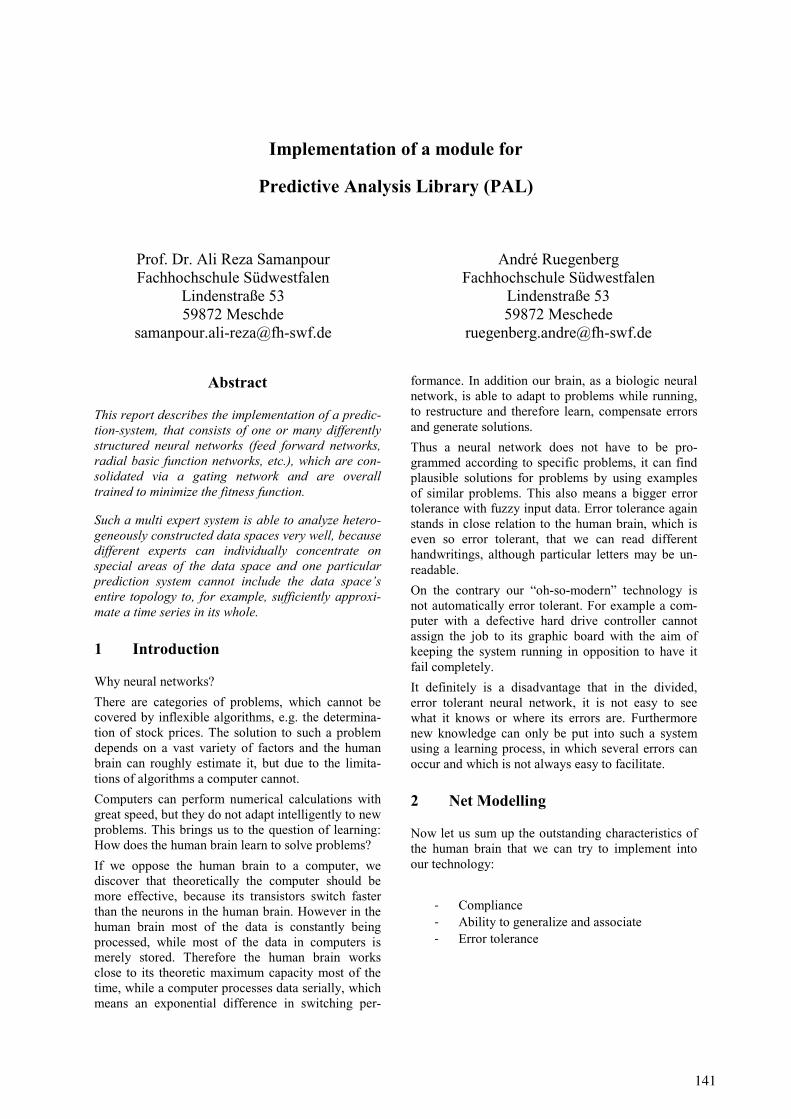
Implementation of a module for

Predictive Analysis Library (PAL)

Prof. Dr. Ali Reza Samanpour Fachhochschule Südwestfalen

Lindenstraße 53 59872 Meschde

[email protected]

André Ruegenberg Fachhochschule Südwestfalen

Lindenstraße 53 59872 Meschede

[email protected]

Abstract

This report describes the implementation of a predic-tion-system, that consists of one or many differently structured neural networks (feed forward networks, radial basic function networks, etc.), which are con-solidated via a gating network and are overall trained to minimize the fitness function.

Such a multi expert system is able to analyze hetero-geneously constructed data spaces very well, because different experts can individually concentrate on special areas of the data space and one particular prediction system cannot include the data space’s entire topology to, for example, sufficiently approxi-mate a time series in its whole.

1 Introduction

Why neural networks? There are categories of problems, which cannot be covered by inflexible algorithms, e.g. the determina-tion of stock prices. The solution to such a problem depends on a vast variety of factors and the human brain can roughly estimate it, but due to the limita-tions of algorithms a computer cannot. Computers can perform numerical calculations with great speed, but they do not adapt intelligently to new problems. This brings us to the question of learning: How does the human brain learn to solve problems? If we oppose the human brain to a computer, we discover that theoretically the computer should be more effective, because its transistors switch faster than the neurons in the human brain. However in the human brain most of the data is constantly being processed, while most of the data in computers is merely stored. Therefore the human brain works close to its theoretic maximum capacity most of the time, while a computer processes data serially, which means an exponential difference in switching per-

formance. In addition our brain, as a biologic neural network, is able to adapt to problems while running, to restructure and therefore learn, compensate errors and generate solutions. Thus a neural network does not have to be pro-grammed according to specific problems, it can find plausible solutions for problems by using examples of similar problems. This also means a bigger error tolerance with fuzzy input data. Error tolerance again stands in close relation to the human brain, which is even so error tolerant, that we can read different handwritings, although particular letters may be un-readable. On the contrary our “oh-so-modern” technology is not automatically error tolerant. For example a com-puter with a defective hard drive controller cannot assign the job to its graphic board with the aim of keeping the system running in opposition to have it fail completely. It definitely is a disadvantage that in the divided, error tolerant neural network, it is not easy to see what it knows or where its errors are. Furthermore new knowledge can only be put into such a system using a learning process, in which several errors can occur and which is not always easy to facilitate.

2 Net Modelling

Now let us sum up the outstanding characteristics of the human brain that we can try to implement into our technology:

- Compliance - Ability to generalize and associate - Error tolerance

141

Figure 1: Artificial neural network (own illustration) But it has to be mentioned that a neural network, which is able to solve any given problem does not exist. There are many different types of networks, learning methods and cases in which they can be used. Every network is bound to its original problem to a certain degree and is therefore able to solve simi-lar problems, but can never replace its natural archi-tecture model.

3 Application Example

We want to teach a neural network a mathematical equation having two input dimensions: z = f(x,y).

Figure 2: Top training data of example of a 3-dimensional function -, below the “learned” out-put (own illustration) mirrored For successful learning it is essential to have plausi-ble data, with which the network can be trained. A training example consists of an exemplary input and a proper output.

4 Training

Now the question is, how this information can be transferred into the network. The Input of a technical neuron has many components, like a biological neu-ron also can have many input signals, basically a vector. It can only have one output signal, which however can be applied to many neurons in the next

layer. This means, that somewhere inside the neuron the many input signals have to be merged to one scalar. Many scalar outputs again build a vector input for another neuron. As in the biology the input data is being merged and, while transiting to the next neu-ron, preprocessed with emphases – this means it gets multiplied by a factor assigning a certain priority to the input data. The priorities that are assigned to the input data are variable, which gives a great dynamic to the network. Therefore the knowledge is mostly being stored and presented including these priorities (p). In consequence a neurons’ output is calculated like this:

𝑦 = 𝑓 ��𝑤𝑖 ∗ 𝑥𝑖𝑖

�

Now the question is, how this information can be transferred into the network. The Input of a technical neuron has many components, like a biological neu-ron also can have many input signals, basically a vector. It can only have one output signal, which however can be applied to many neurons in the next layer. This means, that somewhere inside the neuron the many input signals have to be merged to one scalar. Many scalar outputs again build a vector input for another neuron. As in the biology the input data is being merged and, while transiting to the next neu-ron, preprocessed with emphases – this means it gets multiplied by a factor assigning a certain priority to the input data. The priorities that are assigned to the input data are variable, which gives a great dynamic to the network. Therefore the knowledge is mostly being stored and presented including these priorities (p). In consequence a neurons’ output is calculated like this:

Figure 3: Network error of individual records to Fig. 2

5 Conclusion

Through the complete virtualization for in-memory-environments, in which SAP HANA runs, it is possi-ble to operate many different projects simultaneously and in a significantly more efficient manner.

142

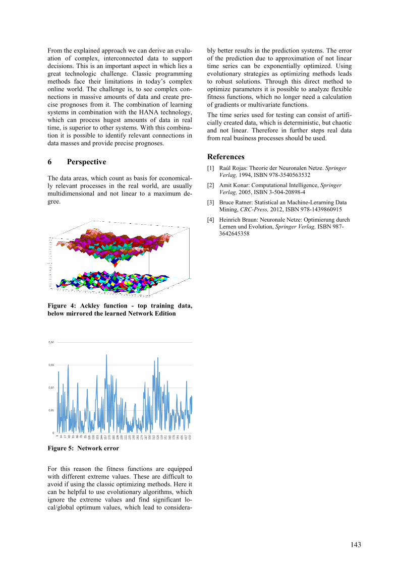
From the explained approach we can derive an evalu-ation of complex, interconnected data to support decisions. This is an important aspect in which lies a great technologic challenge. Classic programming methods face their limitations in today’s complex online world. The challenge is, to see complex con-nections in massive amounts of data and create pre-cise prognoses from it. The combination of learning systems in combination with the HANA technology, which can process hugest amounts of data in real time, is superior to other systems. With this combina-tion it is possible to identify relevant connections in data masses and provide precise prognoses.

6 Perspective

The data areas, which count as basis for economical-ly relevant processes in the real world, are usually multidimensional and not linear to a maximum de-gree.

Figure 4: Ackley function - top training data, below mirrored the learned Network Edition

Figure 5: Network error For this reason the fitness functions are equipped with different extreme values. These are difficult to avoid if using the classic optimizing methods. Here it can be helpful to use evolutionary algorithms, which ignore the extreme values and find significant lo-cal/global optimum values, which lead to considera-

bly better results in the prediction systems. The error of the prediction due to approximation of not linear time series can be exponentially optimized. Using evolutionary strategies as optimizing methods leads to robust solutions. Through this direct method to optimize parameters it is possible to analyze flexible fitness functions, which no longer need a calculation of gradients or multivariate functions. The time series used for testing can consist of artifi-cially created data, which is deterministic, but chaotic and not linear. Therefore in further steps real data from real business processes should be used.

References [1] Raúl Rojas: Theorie der Neuronalen Netze. Springer

Verlag, 1994, ISBN 978-3540563532

[2] Amit Konar: Computational Intelligence, Springer Verlag, 2005, ISBN 3-504-20898-4

[3] Bruce Ratner: Statistical an Machine-Lerarning Data Mining, CRC-Press, 2012, ISBN 978-1439860915

[4] Heinrich Braun: Neuronale Netze: Optimierung durch Lernen und Evolution, Springer Verlag, ISBN 987-3642645358

143

Next Generation Sequencing: From Computational Challenges toBiological Insight

Cornelius [email protected]

Annabell [email protected]

Dr. Sascha SauerMax Planck Institut for Molecular Genetics, Nutrigenomics and Gene Regulation

Otto-Warburg-LaboratoryIhnestrasse 63-73, 14195 Berlin

[email protected]

Abstract

In this project age-associated and inflammatorypathologies shall be studied using approachessuch as chromatin immunoprecipitation (ChIP-seq)and transcriptome profiling (RNA-seq) coupled tonext generation sequencing (NGS) technologies.While NGS enables profound analyses of biologicalprocesses, the main bottleneck remains in thecomputational analysis and interpretation of thegenerated data. Using Future SOC Lab resourceswe established a computational pipeline for RNA-seq(Fall 2012) and ChIP-seq (Spring 2013) data analysis.The utilized DL980 G7 server worked robustly andfacilitating fast analysis of large data sets.

1 Project idea

In the laboratory we exposed cultured cells for adefined period of time to a mild stress-inducingagent. DNA obtained from these experiments wassubjected to chromatin immunoprecipitation (ChIP).Combining ChIP with next generation sequencing(NGS) technology enables thorough determination oftreatment-induced changes (for any protein of interest)in the DNA-protein interaction on a genome-widescale. In the past years a basic ChIP-seq analysespipeline was established, which can be altered inmultiple ways and thus accustomed to individualneeds. Using Future SOC Lab resources we wereable to establish and make use of a highly flexibleand ultra-fast ChIP-seq analysis pipeline. Thisapproach provided the initial framework for theanalyses of future NGS-generated samples. Hence,further participation in the HPI Future SOC Lab wouldenable us to investigate stress-induced genome-widechanges involved in age-associated pathologies andinflammatory processes.

2 Used Resources

Having collaborated with the HPI Future SOC Lab forthe third consecutive term, we were able to work onthe same hardware environment; most changes weremade on the software layer.

2.1 Hardware

As in the previous terms, we worked on a HewlettPackard DL980 G7 server equipped with eight8-core Intel Xeon X7560 processors and 2048 GBof DDR3-1066 main memory. Since the IntelXeon X7560 provides Hyper-threading, 128 logicalprocessors were available for data analysis. Thisproved to be a very powerful system, perfectly suitingour purposes.

2.2 Software

Ubuntu Server 12.04.2 LTS was used as an operatingsystem. Due to recent software updates concerningChIP-Seq analysis, new versions of Bowtie 2 (aligner)and MACS (peak caller) were utilized.

3. Methods and tools

For ChIP-Seq analysis, the pipeline depicted in figure1 was used. In brief, Illumina HiSeq 2500 outputwas aligned to the human reference genome February2009 assembly (GRCh37/hg19) [2] using Bowtie 1[4] (version 1.0.0) or Bowtie 2 [3] (version 2.1.0).After converting aligned reads from ASCII-basedSAM to binary BAM format, output files weresorted and indexed using SAMtools [5] (version0.1.19). For reasons of additional condensationand subsequent visualization in the UCSC GenomeBrowser, sorted BAM files were converted to binarybigWig format via the ASCII-based wiggle track

145

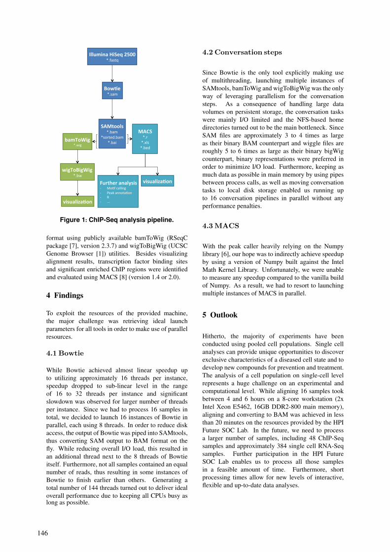
Illumina(HiSeq(2500(*.fastq(

Bow3e(*.sam(

SAMtools(*.bam(

*sorted.bam(*.bai(bamToWig(

*.wig(

wigToBigWig(*.bw(

visualiza3on(

MACS(*.r(*.xls(*.bed(

Further(analysis(4  Mo6f(calling(4  Peak(annota6on(4  R(4  ...(

visualiza3on(

Figure 1: ChIP-Seq analysis pipeline.

format using publicly available bamToWig (RSeqCpackage [7], version 2.3.7) and wigToBigWig (UCSCGenome Browser [1]) utilities. Besides visualizingalignment results, transcription factor binding sitesand significant enriched ChIP regions were identifiedand evaluated using MACS [8] (version 1.4 or 2.0).

4 Findings

To exploit the resources of the provided machine,the major challenge was retrieving ideal launchparameters for all tools in order to make use of parallelresources.

4.1 Bowtie

While Bowtie achieved almost linear speedup upto utilizing approximately 16 threads per instance,speedup dropped to sub-linear level in the rangeof 16 to 32 threads per instance and significantslowdown was observed for larger number of threadsper instance. Since we had to process 16 samples intotal, we decided to launch 16 instances of Bowtie inparallel, each using 8 threads. In order to reduce diskaccess, the output of Bowtie was piped into SAMtools,thus converting SAM output to BAM format on thefly. While reducing overall I/O load, this resulted inan additional thread next to the 8 threads of Bowtieitself. Furthermore, not all samples contained an equalnumber of reads, thus resulting in some instances ofBowtie to finish earlier than others. Generating atotal number of 144 threads turned out to deliver idealoverall performance due to keeping all CPUs busy aslong as possible.

4.2 Conversation steps

Since Bowtie is the only tool explicitly making useof multithreading, launching multiple instances ofSAMtools, bamToWig and wigToBigWig was the onlyway of leveraging parallelism for the conversationsteps. As a consequence of handling large datavolumes on persistent storage, the conversation taskswere mainly I/O limited and the NFS-based homedirectories turned out to be the main bottleneck. SinceSAM files are approximately 3 to 4 times as largeas their binary BAM counterpart and wiggle files areroughly 5 to 6 times as large as their binary bigWigcounterpart, binary representations were preferred inorder to minimize I/O load. Furthermore, keeping asmuch data as possible in main memory by using pipesbetween process calls, as well as moving conversationtasks to local disk storage enabled us running upto 16 conversation pipelines in parallel without anyperformance penalties.

4.3 MACS

With the peak caller heavily relying on the Numpylibrary [6], our hope was to indirectly achieve speedupby using a version of Numpy built against the IntelMath Kernel Library. Unfortunately, we were unableto measure any speedup compared to the vanilla buildof Numpy. As a result, we had to resort to launchingmultiple instances of MACS in parallel.

5 Outlook

Hitherto, the majority of experiments have beenconducted using pooled cell populations. Single cellanalyses can provide unique opportunities to discoverexclusive characteristics of a diseased cell state and todevelop new compounds for prevention and treatment.The analysis of a cell population on single-cell levelrepresents a huge challenge on an experimental andcomputational level. While aligning 16 samples tookbetween 4 and 6 hours on a 8-core workstation (2xIntel Xeon E5462, 16GB DDR2-800 main memory),aligning and converting to BAM was achieved in lessthan 20 minutes on the resources provided by the HPIFuture SOC Lab. In the future, we need to processa larger number of samples, including 48 ChIP-Seqsamples and approximately 384 single cell RNA-Seqsamples. Further participation in the HPI FutureSOC Lab enables us to process all those samplesin a feasible amount of time. Furthermore, shortprocessing times allow for new levels of interactive,flexible and up-to-date data analyses.

146

References

[1] W. J. Kent, C. W. Sugnet, T. S. Furey, K. M. Roskin,T. H. Pringle, A. M. Zahler, and D. Haussler. Thehuman genome browser at ucsc. Genome research,12(6):996–1006, 2002.

[2] E. S. Lander, L. M. Linton, B. Birren, C. Nusbaum,M. C. Zody, J. Baldwin, K. Devon, K. Dewar, M. Doyle,W. FitzHugh, et al. Initial sequencing and analysis ofthe human genome. Nature, 409(6822):860–921, 2001.

[3] B. Langmead and S. L. Salzberg. Fast gapped-readalignment with bowtie 2. Nature methods,9(4):357–359, 2012.

[4] B. Langmead, C. Trapnell, M. Pop, S. L. Salzberg,et al. Ultrafast and memory-efficient alignment of shortdna sequences to the human genome. Genome Biol,10(3):R25, 2009.

[5] H. Li, B. Handsaker, A. Wysoker, T. Fennell, J. Ruan,N. Homer, G. Marth, G. Abecasis, R. Durbin, et al.The sequence alignment/map format and samtools.Bioinformatics, 25(16):2078–2079, 2009.

[6] T. E. Oliphant. Python for scientific computing.Computing in Science & Engineering, 9(3):10–20,2007.

[7] L. Wang, S. Wang, and W. Li. Rseqc: qualitycontrol of rna-seq experiments. Bioinformatics,28(16):2184–2185, 2012.

[8] Y. Zhang, T. Liu, C. A. Meyer, J. Eeckhoute, D. S.Johnson, B. E. Bernstein, C. Nusbaum, R. M. Myers,M. Brown, W. Li, et al. Model-based analysis ofchip-seq (macs). Genome Biol, 9(9):R137, 2008.

147

Detecting biogeographical barriers - testing and putting beta diversity on a

map

Johannes Penner

Museum für Naturkunde, Leibniz-Institute

for Evolution & Biodiversity Research,

Department of Research, Herpetology

Group

Invalidenstrasse 43


[email protected]

Moritz Augustin

Technische Universität Berlin, Department

of Software Engineering & Theoretical

Computer Science, Neural Information

Processing Group

Marchstr. 23


[email protected]

Abstract

Biogeographical regions are not only of scientific but

also of conservation importance. The most common

approach is to map species richness. However, beta

diversity (species turnover) is better suited to identify

where boundaries between regions are.

We calculated beta diversity for West African am-

phibians on a fine scale (30 arcseconds), using mov-

ing window and parallelization techniques. This

would have been impossible with standard hard- and

software. Not only was this the first time to produce

such fine scaled maps but we systematically com-

pared different indices and different moving window

sizes.

Currently our results are only preliminary, the work

plan has not been fulfilled yet and detailed analyses

are pending. Furthermore we would like to ask for an

extension of access possibilities and enhance our

study significantly by switching from binary input

data to proxies for abundance data.

1 Background

Amphibians form an integral part of biodiversity and

are one of the most threatened vertebrate groups on

the globe, with more than one third of all known

species listed as threatened on the IUCN Red List [1,

2]. Biodiversity is declining in many areas and in-

cludes amphibians. The so called amphibian decline

is a global problem and due to a number of reasons.

The main ones are habitat destruction, alteration and

fragmentation as well as pesticides, climate change,

overharvesting and emerging diseases [3]. Causes are

also often interacting. Thus, well-informed conserva-

tion decisions are needed, especially for areas which

harbor the highest diversity but are poorly studied,

i.e. the tropical regions. One base for such decisions

is the answer to where and why species occur.

In general, amphibian diversity and biodiversity are

measured on three different scales: genes, organisms

and landscapes. Organismic diversity is the most

common measure. Measured at one site it is called

alpha diversity, the comparison between two sites is

named beta diversity and gamma diversity is calcu-

lated across a landscape [4].

Besides the general interest where the highest species

diversity is found, the distribution of diversity is

important for conservation. One main aim is to set

priority areas when efforts have to be concentrated.

Another aim is to provide decision makers with the

scientific sound arguments for areas in need of pro-

tection.

In general, a trade-off exists between the conserva-

tion side which requests fine grained maps and the

scientific need to cover large areas. Studies fulfilling

both requirements, covering a large area with a high

resolution, are scarce. Our study is one of the few

attempts to provide both. We study West African

amphibians, which are unique and face multiple

threats; mainly severe habitat destruction and frag-

mentation (e.g. see [5]).

2 Previous work

We used Environmental Niche Modelling (ENM;

also commonly called Species Distribution Model-

ling) to derive the occurrence of West African am-

phibians on a grid of 30x30 arcseconds (≈ 1km²). So

far ENMs were constructed for 158 out of ca. 180

known species with more than 9000 occurrence rec-

ords. The ENMs used 18 environmental parameters:

ten climate (different temperature and precipitation

149

measures), five vegetation (different wavelengths

from two satellites), two altitudinal (calculated from

a digital elevation model and one “hydrology” pa-

rameters) (compare to [6]). A machine learning max-

imum entropy algorithm [7, 8, 9] compared environ-

mental parameters at sites of occurrences against

randomly sampled background data (see [10] for a

statistical explanation of the algorithm). This resulted

in a map showing the distribution of modeled species

richness covering the whole West African region

(Penner et al. in prep.).

3 Project idea

Inspired by McKnight et al. [11] we wanted to inves-

tigate species turnover (≈ beta diversity) for the

whole region. The main aim is to identify biogeo-

graphical regions and boundaries, which are reflected

by relatively high species turnover. This is done by

comparing species occurrences between neighboring

grid cells.

To our knowledge this approach has never been tack-

led systematically, especially with real data, contrary

to simulated data. No agreement exists for example

which index should be used though some progress

has been made. Therefore we will compare different

indices and different moving window sizes.

Another aspect of biological diversity is species rich-

ness (≈ alpha diversity). We will compute different

species richness measures and compare the model

results with established maps used in biological con-

servation projects.

The final programmed software will be open source

published using a public domain license. It will allow

the user to specify own indices and moving window

sizes.


The large scale of our analysis does not permit the

use of available standard computer hard- and soft-

ware. Applying a moving window approach we uti-

lized the HPI Future SOC Lab Fujitsu RX600S5

machines, parallelizing data. Though it would be

interesting to test how the Hewlett Packard DL980

G7 servers would speed up calculations.

5 Findings

Currently we programmed two binary indices Jaccard

[12] and Mountford [13]. Beta diversity is calculated

as the species turn over between one grid cell and its

neighboring cells. A third index, Raup-Crick [14], is

currently being implemented. All three indices use

binary occurrence data and weigh presence and ab-

sence data differently (see [15]). Moving window

sizes varied from 3 to 93 (Mountford) and 201 (Jac-

card). Larger sizes will be explored but are computa-

tionally very intensive.

150

Unique areas are consistently showing up regardless

of the index and the moving window size. Prelimi-

nary analyses indicate that biogeographic barriers

might correspond to major river systems in the re-

gion. However, at the current, stage proper conclu-

sions are premature.

Figure 1 (from previous page): Example of frequency histograms of two different beta diversity indices with two different moving window sizes. From top to bottom (index name & moving window size): Jaccard 3x3, Jaccard 93x93, Mountford 3x3, Mountford 93x93.

Figure 1 shows four examples of frequency histo-

grams for two indices (Jaccard & Mountford) and

two different moving window sizes (3x3 & 93x93).

The non-metric properties of the Mountford index are

clearly visible. It is obvious that both factors are

important. More thorough analyses will be prepared.

Recently, we have additionally computed alpha

diversity both for binary data (species occurence

count) and abundance data (exponential Shannon

entropy). The preliminary results reveal significant

areas of high species richness which have not been

found by previous coarse-grained diversity

estimation. However, more detailed investigations

are necessary to make robust conclusions.

6 Next steps

Our previous runs were successful. Due to delays in

the start of the project, analyses have not been com-

pleted yet and time and logistical constraints did not

allow us to finish all intended runs. As mentioned

above the third index awaits implementation.

In addition, we have discovered a solution to move

the analyses even one large step further. So far we

used binary data, resulting in relatively simple spe-

cies richness maps. This was a result of the current

work flow but has many theoretical disadvantages.

Therefore, we would like to use proxies for abun-

dance. This would open a completely new window,

incorporating such measures as heterogeneity and

evenness in our analyses and potentially a much

higher precision. Using “abundance” data, different

indices are needed. Five potential candidates are:

Shannon, Whittaker, Wilson & Shmida, NESS and

CqN which weigh evenness differently (e.g. see [16]).

Furthermore, using the likelihoods gained from the

ENMs enables us to calculate alpha diversity anew,

also incorporating heterogeneity and evenness. Alt-

hough the preliminary results regarding species rich-

ness look very promising a general conclusion is not

yet possible. Therefore we want to investigate this

measure in more detail and relate it to previous find-

ings.

7 Extension request

So far the possibilities of the HPI Future SOC Lab

not only enabled our work but also took it a huge step

forward. As mentioned above not all analyses were

finalized yet and they should be further improved. A

further use of the HPI Future SOC Lab facilities

would help us tremendously. Therefore we would be

very grateful if an extension of our access to the HPI

Future SOC Lab resources is granted. A follow-up

proposal has been submitted.

8 Acknowledgements

We thank the innumerous colleagues who shared

their data. We are also indebted to a number of peo-

ple who assisted in the field, in the laboratory and in

various other ways, the most important ones are:

Mark-Oliver Rödel, Jakob Fahr, Matthias Herkt,

Günther Barnikel, Mirjana Bevanda, Mareike Hirsch-

feld, Jenja Kronenbitter, Anja Pfahler, Meike

Mohneke & K. Eduard Linsenmair. Various funding

agencies enabled the work. The main part of it was

initially funded by the German Ministry for Educa-

tion and Research (BMBF): BIOTA West Africa, 01

LC 0617J.

We are very grateful to the HPI Future SOC Lab for

granting us access to their computing capacities!

References

[1] S.N. Stuart, , J.S. Chanson, N.A. Cox, B.E. Young,

A.S.L. Rodrigues, D.L. Fischman, & R.W. Waller:

Status and trends of amphibian declines and extinc-

tions worldwide. Science, 306: 1783-1786, 2004.

[2] IUCN: The IUCN Red List of threatened species.

Version 2012.2. http://www.iucnredlist.org. Last ac-

cessed 17th October 2012.

[3] S.N. Stuart, M. Hoffmann, J.S. Chanson, N.A. Cox,

R.J. Berridge, P. Ramani & B.E. Young: Threatened

amphibians of the world. Lynx Edicions, Barcelona,

IUCN, Gland, Switzerland; and Conservation Interna-

tional, Arlington, TX, 2008.

[4] A.E. Magurran: Measuring biological diversity.

Blackwell Publishers, Oxford, 2003.

[5] J. Penner, M. Wegmann, A. Hillers, M. Schmidt &

M.-O. Rödel: A hotspot revisited – a biogeographical

analysis of West African amphibians. Diversity and

Distributions, 17: 1077-1088, 2011.

[6] S.J. Phillips, M. Dudík & R.E. Schapire: A maximum

entropy approach to species distribution modeling. In:

C. Brodley, Editor. Proceedings of the Twenty-First

International Conference on Machine Learning. New

York, ACM Press: 655-662, 2004

[7] S.J. Phillips, R.P. Anderson & R.E. Schapire: Maxi-

mum entropy modeling of species geographic distribu-

tions. Ecological Modelling, 190: 231-259, 2006.

[8] S.J. Phillips & M. Dudík: Modeling of species distri-

butions with Maxent: new extensions and a compre-

hensive evaluation. Ecography, 31: 161-175, 2008.

151

[9] J. Penner, G.B. Adum, M.T. McElroy, T. Doherty-

Bone, M. Hirschfeld, L. Sandberger, C. Weldon, A.A.

Cunningham, T. Ohst, E. Wombwell, D.M. Portik, D.

Reid, A. Hillers, C. Ofori-Boateng, W. Oduro, J. Plöt-

ner, A. Ohler, A.D. Leaché & M.-O. Rödel: West Af-

rica - A safe haven for frogs? A sub-continental as-

sessment of the Chytrid fungus (Batrachochytrium

dendrobatidis). PLoS ONE, 8: e56236, 2013.

[10] J. Elith, S.J. Phillips, T. Hastie, M. Dudík, Y.E. Chee

& C.J. Yates: A statistical explanation of MaxEnt for

ecologists. Diversity and Distributions, 17: 43-57,

2011.

[11] M.W. McKnight, P.S. White, R.I. McDonald, J.F.

Lamoreux, W. Sechrest, R.S. Ridgley & S.N. Stuart:

Putting beta-diversity on the map: broad scale congru-

ence and coincidence in the extremes. PLoS Biology,

5: e272, 2007.

[12] P. Jaccard: Nouvelles recherches sur la distributionflo-

rale. Bulletin de la Societe Vaudoise Sciénces Natu-

relles, 44: 223-270.

[13] M.D. Mountford: An index of similarity and its appli-

cation to classification problems. In: P.W. Murphy,

editor. Progress in soil zoology. Butterworth, London:

43-50, 1962.

[14] D. Raup, & R.E. Crick: Measurement of faunal simi-

larity in paleontology. Journal of Paleontology, 53:

1213-1227, 1979

[15] P. Legendre & L. Legendre: Numerical Ecology, 2nd

Edition. Elsevier Science B.V., Amsterdam, 1998

[16] A.E. Magurran & B.J. McGill: Biological Diversity –

frontiers in measurement and assessment. University

Press, Oxford, 2011.

152

Maximum Resource Utilization Framework and the Performance vs.

Productivity Tradeoff in Hybrid Parallel Computing

Fahad Khalid




[email protected]

Andreas Polze




[email protected]

Abstract

In our previous reports, we have shown the necessity

and effectiveness of the pipeline pattern for imple-

menting combinatorial algorithms on hybrid parallel

architectures. It was argued that the need for pipelin-

ing in such problems stems from the fact that the out-

put size grows exponentially as a function of the in-

put size. In this report we present further progress in

our research in two major directions: 1) maximum

resource utilization, and 2) using design patterns to

balance the productivity vs. performance tradeoff.

Since the underlying assumption is the use of both

CPU and GPU simultaneously for computation, max-

imum resource utilization implies that not only the

GPU, but all threads on the CPU are also fully uti-

lized for processing. We present an approach that

processes the computational kernel simultaneously

on the CPU and the GPU, keeping all resources oc-

cupied with productive work.

The above mentioned contributions have been ap-

plied to a problem from the domain of computational

biology. Here, we present a generalization of the

approach that makes it applicable to a broader set of

problem classes. We argue that by identifying pat-

terns in the algorithm, it is feasible to decide at de-

sign time which parts of the algorithm should be im-

plemented on which architecture; i.e., CPU or GPU.

We further argue that utilizing this knowledge can

simplify the process of developing applications for

hybrid parallel architectures.

1 Introduction

Hybrid computing architectures can be defined as

those that in addition to the general purpose CPU

processors, employ accelerators (or co–processors)

for performance improvement. Employing accelera-

tors can yield significant performance gains [1]; and

consequently, hybrid architectures are now common-

ly used in HPC. According to the Top500 [2] list of

the fastest supercomputers (published in June 2013),

the top two positions are held by supercomputers

based on hybrid architectures.

Graphical Processing Unit (GPU) is the most com-

monly used general purpose accelerator. Over the

past few years, a multitude of computational kernels

have been ported to GPUs with successful perfor-

mance results. However, there are issues pertaining

to developing codes for hybrid architectures. We

focus on two such issues in this report.

First, much of the research is focused on porting and

optimizing parallel algorithms for execution on

GPUs. A general assumption in such an approach is

that the entire kernel of interest will execute on the

GPU only. In the subsections to follow, we show that

if the kernel can be executed simultaneously on both

the CPU and GPU, a significant performance im-

provement can be gained.

Second, GPU acceleration comes at a cost. GPUs are

built on a massively parallel architecture with a large

number of compute cores. However, as compared to

the CPU, each GPU core supports a rather simplistic

feature set. Moreover, GPU caches are much smaller

than that of the CPU. Differences like these limit the

types of kernels that can gain significant performance

improvement by a straight forward port to the GPU.

For a large number of computational problems, a

straight forward port to the GPU does not result in

substantial performance improvement.

Even though productivity tools for GPU program-

ming have improved markedly over time, the range

of features provided by these tools is far narrower

than those available for programming CPUs. Much of

the code optimizations are still left to the program-

mer, which increases both the development and

maintenance effort. This leads to the fact that even

though it is possible to accelerate computational ker-

nels using GPUs, it results in a considerable reduc-

tion in productivity.

153

2 Maximum Resource Utilization

2.1 Concept

In this Section, we present our approach for the effi-

cient and effective utilization of all processing re-

sources available in a hybrid parallel architecture [3].

The method presented here is specific to embarrass-

ingly parallel problems.

In a hybrid parallel environment, execution starts

with the CPU, and is delegated to the GPU at certain

points in the control flow. If the computational kernel

in question were to be executed on the GPU only, the

domain decomposition step would constitute distrib-

uting the input data over the available thread blocks.

This is true for datasets small enough that fit in the

GPU memory. For larger datasets, an additional step

would partition data before the data is moved from

the CPU to the GPU memory. Each partition would

then be processed by a corresponding iteration of the

hybrid pipeline [3].

In our maximum resource utilization approach, a

geometric decomposition step is introduced before

partitioning is performed for pipeline execution. At

this stage, the input data is decomposed into two

parts: one for execution on the CPU and the other for

execution on the GPU. The decomposition is per-

formed based on the relative capability of the two

processing devices. E.g., if the GPU is considerably

more powerful than the CPU, only a small part of the

input will be processed by the CPU, while most of

the data will be processed by the hybrid pipeline.

Figure 1: Framework for Maximum Resource

Utilization [3].

As shown in Figure 1, the Maximum Resource Utili-

zation framework spans the hybrid pipeline. The ge-

ometric decomposition is performed by the Parallel

Harness. The Parallel Harness then forks two

threads, i.e., the Device Harness and the Host-only

code. The Device Harness orchestrates the hybrid

pipeline by receiving as input the (generally larger)

part of the input dataset. The Host-only module is an

OpenMP parallel implementation of the computa-

tional kernel. This module can utilize all available

hardware threads for processing the kernel on the

CPU. The Host-only module and the Device Harness

execute in parallel, thereby maximizing resource uti-

lization across the hybrid parallel architecture.

2.2 Results

The hybrid pipeline approach was applied to a kernel

from the domain of Computational Biology. This

kernel is termed as Combinatorial Candidate Gener-

ation. The algorithm has already been successfully

parallelized on both shared-memory [4] and distrib-

uted-memory [5] CPU based architectures. Here, a

hybrid parallel implementation is presented that in-

corporates the Maximum Resource Utilization

framework. Three instances of the kernel were im-

plemented: Serial, CPU-only parallel and hybrid

pipeline. Figure 2Performance comparison between

the three implementation against four E.Coli datasets.

presents the execution times of the three different

implementations, against four different datasets. The

datasets represent real metabolic networks from the

bacterium E.Coli.

Figure 2: Performance comparison between the

three implementation against four E.Coli datasets.

As can be seen in Figure 2, the CPU-only implemen-

tation outperforms the pipelined implementation on

the first dataset, and the two implementations yield

identical performance on the second dataset. This is

due the fact that these datasets are very small, and the

overhead incurred in pipelining over-shadows much

of the performance gain. For larger datasets however,

the Maximum Resource Utilization approach yields a

significant performance gain, resulting in a 6-fold

speedup over the serial implementation, and 1.8-fold

speedup over the CPU-only parallel implementation.

Figure 2 provides us with four data points only. This

is because the real biological datasets tend to suffer

from combinatorial explosion beyond these four data

points. In order to gain further statistically valid evi-

dence of performance improvements gained by using

the Maximum Resource Utilization framework, the

code was executed against nine artificially created

datasets. These datasets require the same computa-

tional procedure. However, they make it possible to

control the problem size and avoid combinatorial

explosion. The results from the artificially generated

datasets are presented in Figure 3.

154

Figure 3: Performance comparison between the

three implementations against artificially generat-

ed datasets.

3 Design Patterns for Performance vs.

Productivity Tradeoff

This Section presents our analysis toward the gener-

alization of the approaches we have developed during

the course of our FutureSOC project. We emphasize

the need for methods that make it possible to improve

the performance vs. productivity tradeoff; i.e., we

need methods that make it possible to leverage the

performance potential of hybrid architectures while

simplifying the development process.

3.1 Existing Solutions

A major improvement in the programmability of

NVIDIA GPUs was made possible by the develop-

ment of the CUDA [6] programming model. Later

on, the OpenCL [7] standard was developed in order

to provide CUDA like capabilities for vendor neutral

accelerator programming. Over time, these advance-

ments led to the following two major approaches for

improving the effective use of hybrid architectures:

1. Accelerated Domain Specific Libraries

2. Compiler based code generation

In terms of effective utilization of the underlying

hybrid architecture, each of the above mentioned

solution approaches has associated drawbacks. Fol-

lowing is a brief summary:

The domain specific libraries are vital for scientific

computing. However, these serve a very specific pur-

pose and cannot be used as building blocks for prob-

lems in other domains. There is room for develop-

ment of libraries that provide mechanisms for coor-

dination between GPUs and CPUs, and simplify the

process of implementing a much larger set of prob-

lems on hybrid architectures.

As for code generation, not all kinds of computations

are suitable for GPU architectures. Therefore, simply

automating the process of code generation does not

guarantee a significant performance gain. For certain

computational kernels, even optimized GPU code

results in wasted clock cycles. Therefore, it is im-

portant that code generation is complemented with

libraries that make it possible to write cross-device

optimized code.

3.2 Design Patterns and Algorithm De-

composition

The design patterns introduced by the Gang of Four

[8] are considered as building blocks for a robust

object oriented design. These patterns provide ab-

stractions from the domain, and make it possible for

design ideas to be used irrespective of the domain.

These however are not sufficient for parallel pro-

gramming. In order to fill this gap, Design Patterns

for Parallel Programming [9] were explicitly pro-

posed, and have gained considerable popularity over

the years.

The design patterns for parallel programming can be

used to identify the data and control flow in a compu-

tational kernel. This makes it possible to see whether

a certain kernel would be suitable for a given archi-

tecture.

3.3 Outlook

It is conjectured here that looking at the problem

from the point of view of design patterns in parallel

computing can lead to effective utilization of hybrid

architectures. Not only does it highlight possibilities

for performance improvement, it also improves pro-

grammer productivity.

For new codes, the patterns and associated con-

straints can be used to decide how the algorithm can

be effectively distributed across the architecture. This

fits into the existing design strategy for parallel pro-

grams. The method presented in this report is just an

added step to an established process.

In the authors’ research, for existing codes, an auto-

mated process will be introduced. A tool will be de-

veloped for the analysis of existing sources. This tool

will provide recommendations on how the algorithm

should be decomposed. An automated tool will re-

quire the representation of patterns and constraints in

a formal language. Also, an efficient implementation

of the hybrid pipeline model will require optimiza-

tion of the control flow graph. Therefore, much

mathematical formalism will be used in future work.

4 Conclusions

With this report, we declare the project “Paralleliza-

tion of Elementary Flux Mode enumeration for

large–scale metabolic network” successfully con-

cluded. Due to the possibility of utilizing high-end

machines at the FutureSOC Lab, this project has

made novel contributions to the fields of Parallel

Computing and Computational Biology. The project

has culminated in an original publication [3].

The major contributions made by this project are:

155

Development of the Hybrid Pipelining ap-

proach, with application to a real-world

problem from the domain of computational

biology.

Development of the Maximum Resource

Utilization framework, with application to a

real-world problem from the domain of

computational biology.

Insights into generalization of the approach

for applicability to the problem of managing

the Performance vs. Productivity tradeoff in

Hybrid Parallel Computing.

Moreover, this project is an example of a successful

interdisciplinary collaboration between the Hasso

Plattner Institute for Software Systems Engineering

and the Max Planck Institute of Molecular Plant

Physiology.

References

[1] Victor W. Lee, Changkyu Kim, Jatin Chhugani,

Michael Deisher, Daehyun Kim, Anthony D.

Nguyen, Nadathur Satish, Mikhail Smelyanskiy,

Srinivas Chennupaty, Per Hammarlund, Ronak

Singhal, and Pradeep Dubey. “Debunking the 100x

gpu vs. cpu myth: an evaluation of throughput com-

puting on cpu and gpu”. In Proceedings of the 37th

annual international symposium on Computer archi-

tecture, pages 451–460. ACM, 2010.

[2] Erich Strohmaier. “TOP500 - TOP500 super-computer”. In SC, page 18. ACM Press, 2006.

[3] Fahad Khalid, Zoran Nikoloski, Peter Tröger, and

Andreas Polze. “Heterogeneous combi-natorial

candidate generation”. In Felix Wolf, Bernd Mohr,

and Dieter Mey, editors, Euro-Par 2013 Par-allel

Processing, volume 8097 of Lecture Notes in

Computer Science, pages 751–762. Springer Berlin

Heidelberg, 2013.

[4] M. Terzer and J. Stelling, “Accelerating the

Computation of Elementary Modes Using Pattern

Trees.” In Algorithms in Bioinformatics. vol. 4175,

P. Bücher and B. Moret, Eds., ed: Springer Berlin /

Heidelberg, 2006, pp. 333-343.

[5] D. Jevremović, C. T. Trinh, F. Srienc, C. P. Sosa,

and D. Boley, “Parallelization of Nullspace

Algorithm for the computation of metabolic path-

ways”. Parallel Computing, vol. 37, pp. 261-278,

2011.

[6] NVIDIA. CUDA C programming guide.

Design Guide. PG-02829-001_v5.0, October 2012.

[7] Khronos OpenCL Working Group. The OpenCL

specification. Standard specification, De-cember

2011.

[8] Erich Gamma, Richard Helm, Ralph John-son,

and John Vlissides. Design Patterns. Addison-

Wesley, 1995.

[9] Kurt Keutzer, Berna L. Massingill, Timothy G.

Mattson, and Beverly A. Sanders. A design pat-tern

language for engineering (parallel) software:

merging the PLPP and OPL projects. 2010.

156

Batch method for efficient resource sharing in real-time multi-GPU systems

Uri Verner

Technion - Israel Institute of Technology Haifa 32000, Israel

[email protected]

Abstract

The performance of many GPU-based systems de-

pends heavily on the effective bandwidth for transfer-

ring data between the processors. For real-time sys-

tems, the importance of data transfer rates may be

even higher due to non-deterministic transfer times

that limit the ability to satisfy response time require-

ments.

We analyze the bandwidth of two multi-GPU system

as a step towards developing an execution method for

data transfers and distributed computations between

the host (CPUs) and multiple devices (GPUs).

Our experiments show that the bandwidth between a

CPU and a GPU, and between GPUs, in a multi-GPU

system is influenced by concurrent data transfers. Our

results show that different multi-GPU systems can

have different bandwidth distribution behavior.

1 Introduction

In high throughput data processing systems, the

computational load is distributed across multiple inter-

connected processors. To efficiently execute data-par-

allel parts of the computation, such systems often

make use of discrete GPUs and other compute accel-

erators. The data is collaboratively processed by the

CPUs and accelerators, and transferred between their

local memories as required by the algorithm.

For real-time systems, where the worst-case execu-

tion time is important, the common methods for re-

source sharing include bandwidth allocation and time

division. The bandwidth allocation method calls to di-

vide the resource into a number of smaller portions,

and to assign each of them to a task. For example, if

the bandwidth of a bus is 8MB/s, it can be distributed

among four tasks so that each task is assigned 2MB/s.

The time division method calls to split the time do-

main into time-slots and to assign them to the tasks

according to a given priority scheme. For example, the

8MB/s bus can be assigned for a period of time to task

A and later to task B. Each of these methods allows

the system to make the communication time determin-

istic at the expense of underutilizing resources such as

the bus bandwidth, since a resource that is assigned to

a task but not fully utilized is not used by the other

tasks. Underutilization of the resources could increase

power consumption or even prevent the system from

meeting real-time deadlines.

In this project we analyze the bandwidth of two

multi-GPU system as a step towards developing an ex-

ecution method for data transfers and distributed com-

putations between the host (CPUs) and multiple de-

vices (GPUs).

Figure 1: System architecture of a multi-GPU system

157

Our experiments show that the bandwidth between

a CPU and a GPU, and between GPUs, in a multi-GPU

system is influenced by concurrent data transfers. Our

results show that different multi-GPU systems can

have different bandwidth distribution behavior.

2 System architecture

In this work, we will focus on a single-node multi-

GPU system that includes one or more CPUs and a set

of discrete GPUs, each of which has a local memory

module and serves as a computational device. Figure

1 illustrates a possible architecture of such a system.

The interconnect provides connectivity among the dif-

ferent components such as memories, processors,

GPUs, etc., and consists of several communication do-

mains, depicted in the figure by background blocks.

Each domain consists of components that use the same

architecture and protocol for communication. The do-

mains are bridged by components that belong to sev-

eral domains.

As the figure shows, the system consists of memory

modules (MEM), CPUs, GPUs, and I/O Hubs (IOH).

The I/O hubs bridge between the processor intercon-

nect and PCI Express, and provide connectivity be-

tween PCI Express devices and the main memory

modules; in some architectures, the I/O hubs are inte-

grated into the CPUs. In addition to GPUs, other ex-

ternal devices may be connected via PCI Express; ex-

amples include compute accelerators such as Intel's

Xeon Phi and high-throughput network cards. In this

work, we focus on GPU-based systems, but the pro-

posed method can be extended to be used with other

devices as well.

Each CPU accesses its local memory directly via

the memory bus, while distant CPUs and I/O Hubs

(IOH) access it indirectly via the processor intercon-

nect, which is a set of high bandwidth full-duplex

point-to-point links. Examples of such interconnects

include Intel QuickPath Interconnect (QPI) and Hy-

perTransport.

Data transfers from and to GPU memory are exe-

cuted by DMA controllers (a.k.a. DMA engines).

GPUs that have two DMA controllers support bi-di-

rectional data transfer, while GPUs that have a single

DMA can transfer data only in one direction at a time.

GPUs from the same PCI Express domain can ex-

change data directly, while most systems do not sup-

port direct data transfer between GPUs in different do-

mains due to chipset limitations. A common solution

for transferring data between GPUs that reside in dif-

ferent domains, is to stage the data in CPU memory,

using two DMA controllers.

3 Evaluation

To evaluate the batch method, we consider two appli-

cations running on two multi-GPU systems. We com-

pare the batch method with two other bandwidth dis-

tribution methods: bandwidth allocation and time di-

vision.

For each system, we provide the system specification,

find and analyze the effective bandwidth, and compare

the performance using each of the methods in test case

applications.

We describe two existing systems and usetwo existing

techniques to analyze their effective bandwidth.

3.1 Nehalem multi-GPU system

This system is a Tyan FT72B7015 server featuring the

following components:

1. Two 4-core Intel Xeon 5620 CPUs at

2.4GHz, based on the Nehalem micro-archi-

tecture

2. An Intel 5520/ICH10R chipset with a QPI

processor interconnect at 4.8GT/s (9.6GB/s)

and two I/O hubs, each with two PCIe 2.0

ports

3. A total of 24GB RAM in two modules

4. Four NVIDIA Tesla C2050 GPUs, each with

3GB of GDDR 5 memory

The system runs Ubuntu 10.04 x64 Linux with CUDA

SDK 5.0.

Analyzing effective bandwidth

The results show that the bus bandwidth is asymmet-

ric; the effective H2D PCIe bandwidth is between 25%

and 50% higher than the D2H bandwidth. We also see

that the effective bandwidth to the remote GPUs is

20% lower. Since the QPI bus has higher bandwidth

than the PCIe bus, this indicates that the latency of the

extra hop over QPI translates into throughput degrada-

tion. The H2D aggregate bandwidth scales up for two

GPUs by 57% for local GPUs (saturates the QPI bus),

and by 33% for remote GPUs. In contrast, the D2H

bandwidth for two GPUs does not scale. For four

GPUs, the H2D bandwidth does not scale further, but

the aggregate D2H bandwidth lines up with the band-

width of the local GPUs. We ascribe the reduced scal-

ing to chipset limitations, except where the QPI bus

was saturated. Since the GPUs only have one DMA

engine, they are not able to get more bandwidth from

bi-directional transfer, yet we see that for the local

GPUs a bi-directional transfer is faster than an H2D

transfer followed by a D2H.

3.2 Sandy Bridge multi-GPU system

This system features the following components:

158

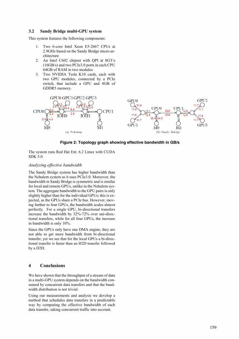
1. Two 6-core Intel Xeon E5-2667 CPUs at

2.9GHz based on the Sandy Bridge micro-ar-

chitecture

2. An Intel C602 chipset with QPI at 8GT/s

(16GB/s) and two PCIe3.0 ports in each CPU

64GB of RAM in two modules

3. Two NVIDIA Tesla K10 cards, each with

two GPU modules, connected by a PCIe

switch, that include a GPU and 4GB of

GDDR5 memory.

The system runs Red Hat Ent. 6.2 Linux with CUDA

SDK 5.0.

Analyzing effective bandwidth

The Sandy Bridge system has higher bandwidth than

the Nehalem system as it uses PCIe3.0. Moreover, the

bandwidth in Sandy Bridge is symmetric and is similar

for local and remote GPUs, unlike in the Nehalem sys-

tem. The aggregate bandwidth to the GPU pairs is only

slightly higher than for the individual GPUs; this is ex-

pected, as the GPUs share a PCIe bus. However, mov-

ing further to four GPUs, the bandwidth scales almost

perfectly. For a single GPU, bi-directional transfers

increase the bandwidth by 32%-72% over uni-direc-

tional transfers, while for all four GPUs, the increase

in bandwidth is only 10%.

Since the GPUs only have one DMA engine, they are

not able to get more bandwidth from bi-directional

transfer, yet we see that for the local GPUs a bi-direc-

tional transfer is faster than an H2D transfer followed

by a D2H.

4 Conclusions

We have shown that the throughput of a stream of data

in a multi-GPU system depends on the bandwidth con-

sumed by concurrent data transfers and that the band-

width distribution is not trivial.

Using our measurements and analysis we develop a

method that schedules data transfers in a predictable

way by computing the effective bandwidth of each

data transfer, taking concurrent traffic into account.

Figure 2: Topology graph showing effective bandwidth in GB/s

3.2 Sandy Bridge multi-GPU system

This system features the following components:

159

SAP HANA in a Hybrid Main Memory Environment

Ahmadshah Waizy [email protected]

Ralf Liesegang [email protected]

Konrad Büker [email protected]

Dieter Kasper [email protected]

Jürgen Schrage [email protected]

Fujitsu Technology Solutions GmbH Heinz-Nixdorf-Ring 1

33106 Paderborn, Germany

Bernhard Höppner [email protected]

Ole Lilienthal [email protected]

Henning Schmitz [email protected]

SAP Innovation Center Potsdam Prof.-Dr.-Helmert-Str. 2-3 14482 Potsdam, Germany

Abstract

Hybrid main memory environments refer to the in-troduction of a further memory level to today’s hardware architectures, which offers a fine-granular distinction of data and introduces new possibilities for applications. Storage Class Memory (SCM) as a feasible memory sublayer introduces a new class of memory technologies, which is well suited to increase the memory capabilities of individual servers effi-ciently by combining byte granular access, low laten-cies, high data density and non-volatility. We concentrate on potential applications of a hybrid main memory environment in the area of in-memory computing databases. We focus on evaluating SAP HANA concerning the usage of SCM for analytical data processing. As SCM prototypes are not yet available physically, a hybrid main memory envi-ronment is integrated into Linux by emulating the speed of data access as expected in future SCM tech-nology. This second memory layer has been made available in SAP HANA and is used as the database component for storing relational data in-memory. A common benchmark comparing multiple SCM con-figurations was executed and the results are present-ed in this document. This project was executed at the Future SOC Lab of the Hasso-Plattner-Institute in Potsdam, Germany, and utilized infrastructure available in the lab.

1 Introduction

The clear distinction of memory and storage in to-day’s software architectures will potentially be

blurred by the introduction of Storage Class Memory (SCM). SCM brings together the characteristics of available storage solutions like Hard Disks (HDD) or Solid-State Drives (SSD) with existing memory tech-nologies such as Dynamic Random Access Memory (DRAM). This upcoming class of memory combines non-volatility and low power consumption, allowing low access latencies and still offers high data density. A classification of SCM latencies compared with existing storage and memory solutions can be found in Figure 1. SCM can be implemented in hardware by for example Phase-change Random Access Memory (PCRAM) and Resistive Random Access Memory (ReRAM) which are both not expected to be availa-ble before 2016. Bridge technologies overcoming this period in time will be available as of 2014 and will be sufficient to cover specific characteristics of SCM.

Figure 1: Latency characteristics of different types of data storage media

161

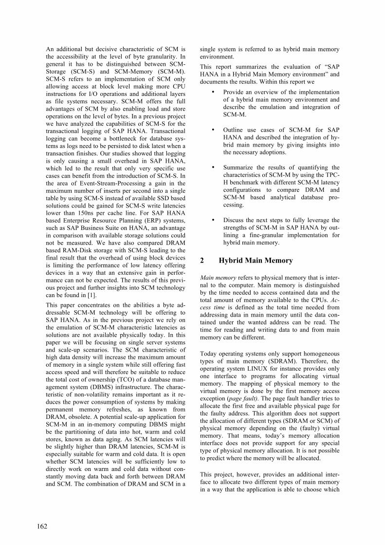
An additional but decisive characteristic of SCM is the accessibility at the level of byte granularity. In general it has to be distinguished between SCM-Storage (SCM-S) and SCM-Memory (SCM-M). SCM-S refers to an implementation of SCM only allowing access at block level making more CPU instructions for I/O operations and additional layers as file systems necessary. SCM-M offers the full advantages of SCM by also enabling load and store operations on the level of bytes. In a previous project we have analyzed the capabilities of SCM-S for the transactional logging of SAP HANA. Transactional logging can become a bottleneck for database sys-tems as logs need to be persisted to disk latest when a transaction finishes. Our studies showed that logging is only causing a small overhead in SAP HANA, which led to the result that only very specific use cases can benefit from the introduction of SCM-S. In the area of Event-Stream-Processing a gain in the maximum number of inserts per second into a single table by using SCM-S instead of available SSD based solutions could be gained for SCM-S write latencies lower than 150ns per cache line. For SAP HANA based Enterprise Resource Planning (ERP) systems, such as SAP Business Suite on HANA, an advantage in comparison with available storage solutions could not be measured. We have also compared DRAM based RAM-Disk storage with SCM-S leading to the final result that the overhead of using block devices is limiting the performance of low latency offering devices in a way that an extensive gain in perfor-mance can not be expected. The results of this previ-ous project and further insights into SCM technology can be found in [1]. This paper concentrates on the abilities a byte ad-dressable SCM-M technology will be offering to SAP HANA. As in the previous project we rely on the emulation of SCM-M characteristic latencies as solutions are not available physically today. In this paper we will be focusing on single server systems and scale-up scenarios. The SCM characteristic of high data density will increase the maximum amount of memory in a single system while still offering fast access speed and will therefore be suitable to reduce the total cost of ownership (TCO) of a database man-agement system (DBMS) infrastructure. The charac-teristic of non-volatility remains important as it re-duces the power consumption of systems by making permanent memory refreshes, as known from DRAM, obsolete. A potential scale-up application for SCM-M in an in-memory computing DBMS might be the partitioning of data into hot, warm and cold stores, known as data aging. As SCM latencies will be slightly higher than DRAM latencies, SCM-M is especially suitable for warm and cold data. It is open whether SCM latencies will be sufficiently low to directly work on warm and cold data without con-stantly moving data back and forth between DRAM and SCM. The combination of DRAM and SCM in a

single system is referred to as hybrid main memory environment. This report summarizes the evaluation of “SAP HANA in a Hybrid Main Memory environment” and documents the results. Within this report we

• Provide an overview of the implementationof a hybrid main memory environment anddescribe the emulation and integration ofSCM-M.

• Outline use cases of SCM-M for SAPHANA and described the integration of hy-brid main memory by giving insights intothe necessary adoptions.

• Summarize the results of quantifying thecharacteristics of SCM-M by using the TPC-H benchmark with different SCM-M latencyconfigurations to compare DRAM andSCM-M based analytical database pro-cessing.

• Discuss the next steps to fully leverage thestrengths of SCM-M in SAP HANA by out-lining a fine-granular implementation forhybrid main memory.

2 Hybrid Main Memory

Main memory refers to physical memory that is inter-nal to the computer. Main memory is distinguished by the time needed to access contained data and the total amount of memory available to the CPUs. Ac-cess time is defined as the total time needed from addressing data in main memory until the data con-tained under the wanted address can be read. The time for reading and writing data to and from main memory can be different.

Today operating systems only support homogeneous types of main memory (SDRAM). Therefore, the operating system LINUX for instance provides only one interface to programs for allocating virtual memory. The mapping of physical memory to the virtual memory is done by the first memory access exception (page fault). The page fault handler tries to allocate the first free and available physical page for the faulty address. This algorithm does not support the allocation of different types (SDRAM or SCM) of physical memory depending on the (faulty) virtual memory. That means, today’s memory allocation interface does not provide support for any special type of physical memory allocation. It is not possible to predict where the memory will be allocated.

This project, however, provides an additional inter-face to allocate two different types of main memory in a way that the application is able to choose which

162

data to store in what type (SDRAM or SCM) of phys-ical memory area. – We call that mechanism Hybrid Main Memory Support.

From our Hybrid Main Memory Support, the applica-tion, SAP HANA, knows two different types of memory: the one that will contain the entire SAP HANA database and the other one that contains all other program data, e.g. text, bss, data and stack (Hybrid Main Memory). Therefore, SAP HANA will use two different memory allocation calls (malloc and scmalloc) to put the data into these different areas. Figure 2 shows the physical memory split into two parts that is used by SAP HANA. The SCM emulating area of the physical memory (behaving like SCM) is used to store the database, and the remaining rest of the physical memory (be-having like standard SDRAM) is used for application and kernel memory, respectively.

Figure 2: Split and usage of the Physical Main Memory

2.1 Configuration of a Hybrid Main Memory

The main memory is divided into two parts, the emu-lated SCM part and the standard SDRAM part (Hy-brid Main Memory). Figure 3 shows the hybrid main memory configura-tion that was used. The DIMMs attached to CPU 3 and CPU 4 are used for the SCM emulating area. The other part is for standard system use. CPU 3 and CPU 4 are switched off to ensure that no applications are assigned to these CPUs and memory access into the SCM emulating area is never local (fast access).

Figure 3: Physical Main Memory Configuration

2.2 Emulating SCM latencies Latency refers to delays in transmitting data between the CPU and SDRAM. SDRAM latency is often measured in memory bus clock cycles. However, the CPU operates faster than the memory, so the CPU must wait while the proper segment of memory is located and read before the data can be sent back. This also adds to the total SDRAM latency. During power-on self-test (POST) computers auto-matically configure the hardware that is currently present. Serial presence detect (SPD) is a memory hardware feature which lets the computer know what memory is present, and what timings to use to access the memory DIMMs specified. The SPD data of the DIMMs attached to CPU 3 and CPU 4 are writeable and can be changed to return different latency values during POST (Figure 4). We used this technique to emulate different SCM latencies.

Figure 4: CPU/Memory Configuration with adjusta-ble Latencies

The latency definitions are shown in Figure 5. Since the SCM latencies would be multiples of DRAM latencies, our SCM emulation changes the DRAM latency value (tRL) by different factors.

163

Figure 5: Memory Access Latencies

2.3 Enhancements to Virtual Memory Management to Support Hybrid Main Memory

Today’s operating systems (OS) provide only one way to allocate virtual memory for the application: the malloc function. There is no way to instruct mal-loc to use particular pages of physical memory. The OS only knows the location of the physical memory (ccNUMA); besides this there is no differentiation between the physical memory pages. Figure 6 shows the current standard implementation of allocating memory pages for an application.

Figure 6: How memory allocation works today

We have implemented the following memory alloca-tion functions to support hybrid main memory alloca-tion for SAP HANA. By using these additional func-tions the application is enabled to allocate SCM emu-lating memory. The essential requirement of hybrid main memory management is to provide ways to dynamically allocate portions of desired memory (SDRAM or SCM) to programs at their request, and freeing it for reuse when no longer needed.

List of implemented additional functions: • void *scmalloc(size_t);

• int posix_scmemalign(void**,size_t, size_t);• void scmfree(void *);• void *scmrealloc(void *, size_t);

The function scmalloc and the other provided func-tions implement the same, thread-safe API as malloc and similar functions. Using these functions (malloc or scmalloc) an appli-cation is able to choose where the physical memory is to be allocated (SDRAM or emulated SCM). Figure 7 shows the hybrid main memory allocation implementation. The physical pages of the SCM emulating memory are managed by a kernel driver (rscmmap). Memory requested by the function scmalloc will be allocated by rscmmap from the SCM emulating physical pages and will be mapped into the application so that the application addresses SCM emulating memory directly in a byte/word-like manner. The SCM area is reserved upon booting and is no longer available to the normal OS paging sys-tem. This means that the physical memory is allocat-ed into different pools, where each pool represents pages of memory of a certain type, which are man-aged by the Linux paging or rscmmap.

Figure 7: How the system is extended to support hybrid main memory

3 SAP HANA

Since 2010 SAP is offering its in-memory computing appliance SAP HANA, which introduces a technolo-gy that can be used to address problems in the do-main of real-time processing of big data [2, 3]. Besides fundamental aspects like the organization of tables in columns, dictionary encoding and many more, the utilization of main memory as the only data store can be seen as the most significant decision in architectural design. Thus SAP HANA profits from shifting the old performance bottleneck of hard disks to the latency of RAM. Accordingly RAM becomes

164

the key factor when scaling the size of SAP HANA systems. Although the feasible amount of RAM in a single server has increased over the past years, it’s still limiting compared to hard disks. As announced in May 2013 [4] HANA Hawk is today’s largest prototype system offering 12TB of main memory in a single server. Even though this is a big improvement for a single server, databases for business systems like Enterprise Resource Planning (ERP) and Cus-tomer Relationship Management (CRM) systems can exceed this limitation. Customers facing larger amounts of data will be given the opportunity to scale-out their HANA systems. A shared-nothing approach offers the ability to independently spread data across multiple servers increasing the maximum amount of data as well as the computation power of the whole landscape. Nonetheless increasing the size of the data stores comes with a considerable amount of economic effort. Apart from that, new memory technologies such as SCM offer affordable alterna-tives introducing a higher data density compared to DRAM while still offering much higher performance than NAND Flash based solutions such as SSDs. Introducing these solutions to today’s systems pro-vides the opportunity to increase the maximum amount of memory in single server, thus offering new scale-up scenarios. This paragraph concentrates on the capabilities of upcoming memory solutions like SCM, mainly fo-cusing on low latencies and high data density.

3.1 Hybrid Main Memory for SAP HANA Today’s hardware architectures typically comprise three levels of caches, main memory and storage with all of them fulfilling specific tasks. As shown in Figure 1, upcoming hardware technologies addressed by the phrase SCM will change this architecte by introducing another level of memory. Blurring the differences between storage and memory will certain-ly involve the adoption of existing software architec-tures. As we concentrate on the latency and data density characteristics of SCM, it is more likely to describe SCM as a descendant of main memory and introduce the concept of so called hybrid main memory architectures. As described in paragraph 2, we use a main memory based emulation of SCM and introduce a second kind of memory based on this. For application developers SCM is accessible similar to main memory by using the appropriated commands scmalloc, scmrealloc, posix_scmemalign and scm-free. Introducing a second level of memory by pre-serving the availability of main memory makes it possible to distinct parts of the system which need to run on fast DRAM and others which can reside on slower but cheaper solutions. For a database management system such as SAP HANA this distinctions leads to the question how to split data into partitions which is part of the scientific area of data aging. In general data aging partitions data into hot, warm and cold data where data is as-

signed to these groups by classification algorithms. Data classification can be achieved by statistical and manual approaches. Manual classification relies on application specific input while statistical approaches monitor the usage of attributes [5], [6]. Besides data aging hybrid main memory environments are appli-cable to any big data use case. A multi-level memory environment could be used as another caching archi-tecture where SCM serves as big data store and tradi-tional RAM as a subsequent layer. This approach involves additional effort copying data between the different memories and relies on the quality of the implemented caching algorithms. In this paper we concentrate on the question whether it is desirable to directly operate on SCM instead of shifting data between memory layers. This analysis can answer the question of whether or not to directly work with cold or even warm data in SCM. Therefore the impact of slightly higher latencies on the perfor-mance of database operations is the key indicator of our study. The aspect of a hybrid architecture is uti-lized by only applying SCM to the Index Server of SAP HANA, which contains the actual data stores and engines for data processing. All other compo-nents of the database and the whole operating system will be using normal RAM.

3.2 Adoption of SAP HANA First insights into the correlation between memory latencies and database performance can be gained by adopting SAP HANA in order to support the usage of the emulated SCM. HANA consists of the four main components Name Server, Index Server, Statistics Server, and Preprocessor Server. A basis library for memory management is shared between all compo-nents offering an efficient memory pool based man-agement. “This pool of allocated memory is pre-allocated from the operating system over time, up to a predefined global allocation limit, and is then effi-ciently used as needed by the SAP HANA database code.” [7] This pool allocation using normal main memory is executed for all HANA components ex-cept of the Index Server. We have introduced another allocator in HANA allowing the allocation of memory in emulated SCM. As described in paragraph 2.3 memory is also allo-cated in chunks and then used as needed by SAP HANA. The allocation of memory is based on map-ping the emulated SCM devices into the virtual ad-dress space of the appropriate application. This allo-cator is integrated into the basis library of SAP HANA and can be enabled for distinct components by changing environment variables. By specifying appropriate hook functions the behavior of the GNU C Library function malloc, realloc and free as well as the posix C function posix_memalign is redirected to the newly implement SCM allocator. Therefore any allocation of the appropriate database component will be using SCM instead of traditional RAM. We have activated the SCM allocator for the Index Server

165

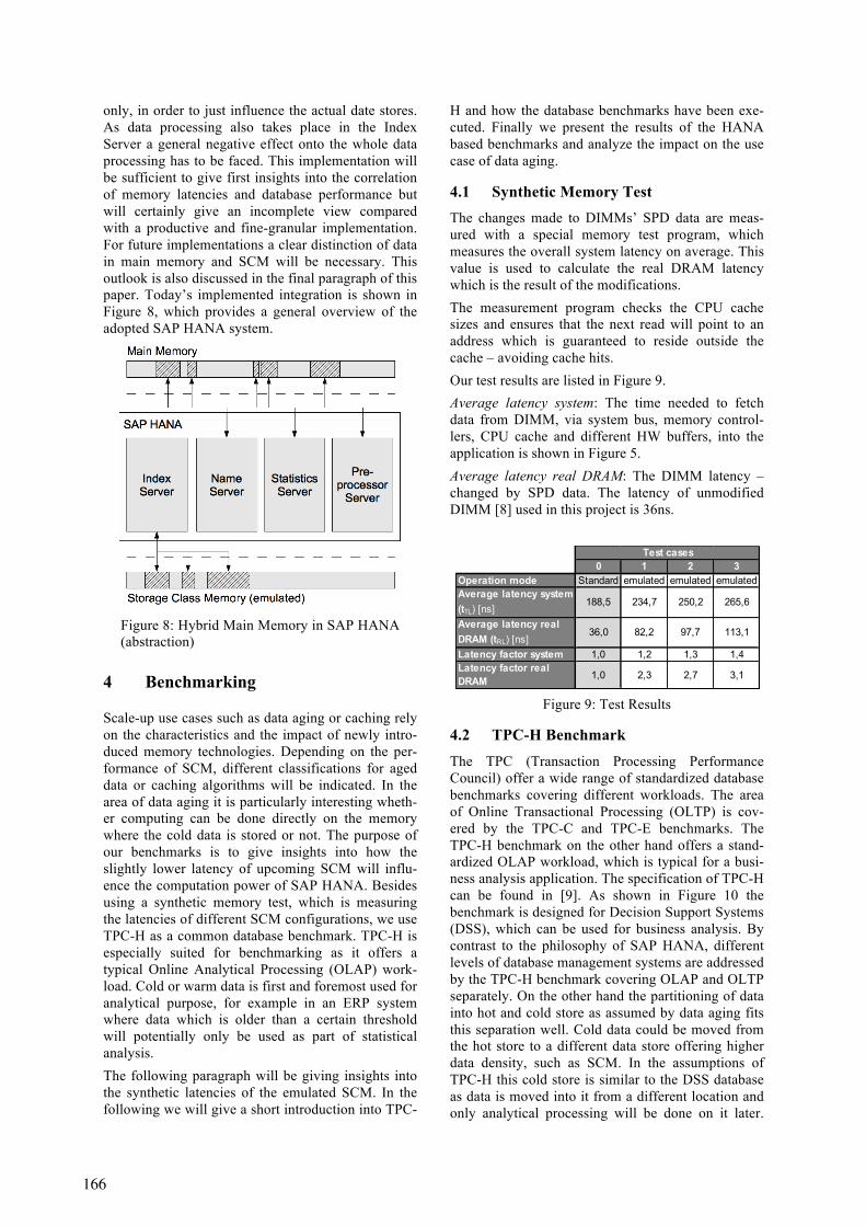
only, in order to just influence the actual date stores. As data processing also takes place in the Index Server a general negative effect onto the whole data processing has to be faced. This implementation will be sufficient to give first insights into the correlation of memory latencies and database performance but will certainly give an incomplete view compared with a productive and fine-granular implementation. For future implementations a clear distinction of data in main memory and SCM will be necessary. This outlook is also discussed in the final paragraph of this paper. Today’s implemented integration is shown in Figure 8, which provides a general overview of the adopted SAP HANA system.

Figure 8: Hybrid Main Memory in SAP HANA (abstraction)

4 Benchmarking

Scale-up use cases such as data aging or caching rely on the characteristics and the impact of newly intro-duced memory technologies. Depending on the per-formance of SCM, different classifications for aged data or caching algorithms will be indicated. In the area of data aging it is particularly interesting wheth-er computing can be done directly on the memory where the cold data is stored or not. The purpose of our benchmarks is to give insights into how the slightly lower latency of upcoming SCM will influ-ence the computation power of SAP HANA. Besides using a synthetic memory test, which is measuring the latencies of different SCM configurations, we use TPC-H as a common database benchmark. TPC-H is especially suited for benchmarking as it offers a typical Online Analytical Processing (OLAP) work-load. Cold or warm data is first and foremost used for analytical purpose, for example in an ERP system where data which is older than a certain threshold will potentially only be used as part of statistical analysis. The following paragraph will be giving insights into the synthetic latencies of the emulated SCM. In the following we will give a short introduction into TPC-

H and how the database benchmarks have been exe-cuted. Finally we present the results of the HANA based benchmarks and analyze the impact on the use case of data aging.

4.1 Synthetic Memory Test The changes made to DIMMs’ SPD data are meas-ured with a special memory test program, which measures the overall system latency on average. This value is used to calculate the real DRAM latency which is the result of the modifications. The measurement program checks the CPU cache sizes and ensures that the next read will point to an address which is guaranteed to reside outside the cache – avoiding cache hits. Our test results are listed in Figure 9. Average latency system: The time needed to fetch data from DIMM, via system bus, memory control-lers, CPU cache and different HW buffers, into the application is shown in Figure 5. Average latency real DRAM: The DIMM latency – changed by SPD data. The latency of unmodified DIMM [8] used in this project is 36ns.

Figure 9: Test Results

4.2 TPC-H Benchmark The TPC (Transaction Processing Performance Council) offer a wide range of standardized database benchmarks covering different workloads. The area of Online Transactional Processing (OLTP) is cov-ered by the TPC-C and TPC-E benchmarks. The TPC-H benchmark on the other hand offers a stand-ardized OLAP workload, which is typical for a busi-ness analysis application. The specification of TPC-H can be found in [9]. As shown in Figure 10 the benchmark is designed for Decision Support Systems (DSS), which can be used for business analysis. By contrast to the philosophy of SAP HANA, different levels of database management systems are addressed by the TPC-H benchmark covering OLAP and OLTP separately. On the other hand the partitioning of data into hot and cold store as assumed by data aging fits this separation well. Cold data could be moved from the hot store to a different data store offering higher data density, such as SCM. In the assumptions of TPC-H this cold store is similar to the DSS database as data is moved into it from a different location and only analytical processing will be done on it later.

0 1 2 3Operation mode Standard emulated emulated emulatedAverage latency system (tTL) [ns]

188,5 234,7 250,2 265,6

Average latency real DRAM (tRL) [ns]

36,0 82,2 97,7 113,1

Latency factor system 1,0 1,2 1,3 1,4Latency factor real DRAM 1,0 2,3 2,7 3,1

Test cases

166

Therefore TPC-H is well suited to evaluate whether memory such as SCM will be suitable to directly work on cold data without copying it back to main memory.

Figure 10: TPC-H Business Environment [9]

As most benchmarks TPC-H consists of two parts, dataset and workload. The schema of the dataset comprises eight tables with some tables having one-to-many relationships between each other. Each table has a predefined size which is depending on the scal-ing factor of the TPC-H benchmark. Using the avail-able generator application the dataset can be created according to the TPC-H specification. Scaling factors out of a predefined set can be selected where scaling factors are about equal to the size of the dataset in gigabytes. According to the available configuration of the hybrid main memory environment and its implementation the highest scaling factor possible in our setup is 100GB. Besides the general dataset addi-tional tables for so-called refresh queries have to be generated. The whole dataset is finally inserted into the database which is then prepared for the bench-mark. The workload of TPC-H, portraying the activity of a wholesale supplier, consists of 22 analytical queries Qi where 1<=i<=22 plus two refresh queries RF1 and RF2. A query set is a sequential execution of all 22 queries. A query stream equals the execution of a single query set by a single emulated user. There are two types of refresh queries where RF1 adds new sales information into the database and RF2 and removes old sales information. A pair of refresh functions consists of one execution of RF1 followed by one execution of RF2. A refresh stream is defined as the sequential execution of an integral number of

pairs of refresh functions. A full TPC-H performance test consists of one power test followed by one throughput test where for our purposes it is sufficient to focus on the TPC-H Power. A power test equals the sequential execution of RF1 followed by all 22 Queries Qi followed by RF2. Therefore it measures the raw query execution power of the system using only a single user. The execution time in seconds for each query and refresh function is recorded. The TPC-H Power metric, which is the query per hour rate, is used to compare DBMS and is defined as

𝑃𝑜𝑤𝑒𝑟 =3600 ∗ 𝑆𝐹

𝑄𝐼(𝑖, 0)!!!!!!! ∗ 𝑅𝐼(𝑗, 0)!!!

!!!!"

4.3 TPC-H using Hybrid Main Memory The correlation of SCM latencies and the perfor-mance of SAP HANA will be the key indicator to evaluate the usage of SCM for cold data. The impact of latencies on database performance will be giving insights into the question if cold data can be directly accessed from a slightly slower but decisively larger storage. We have used the TPC-H Power metric to compare the number of queries per second for differ-ent latencies of the emulated SCM. Figure 11 is visu-alizing the results of the TPC-H Power benchmark in seconds for every refresh query and each of the three different SCM configurations one to three and the initial DRAM latency, which are shown in Figure 9. Besides the total runtime of each benchmark execu-tion we also added the TPC-H Power metric which quantifies the query per hour rate. Additionally, fac-tors comparing latency configuration one to three with the initial configuration zero are provided, which allows the comparability of the configurations.

Figure 11: TPC-H Power results in seconds for all 22 queries and four different configurations of emulated

SCM

167

The benchmark results of the configurations zero to two show increasing runtimes and decreasing TPC-H Power results. Configuration three seems to be devi-ating from this behavior. We will be focusing on results one to two first and analyze the special con-figuration three separately later. The results in Figure 11 outline the correlation of memory latencies and SAP HANA performance. The coefficient of deter-mination of TPC-H Power factors and real DRAM latency factors (compare Figure 9) shows this strong correlation of latencies and performance:

𝑅! = 99,06% This result has been expected as increasing the memory latency has slowed down the whole data store of the in-memory database. On the other hand it is even more interesting to take a closer look onto the resulting regression line in Figure 12.

Figure 12: Latency Factor for DRAM (real) and TPC-H Power Factor including regression line

The regression line shows a gentle negative slope where the linear function looks as follows:

𝑌 = 1,13 − 0,13 ∗ 𝑋 Therefore the increase of memory latencies X is only decreasing the TPC-H Power Factor Y by 0,13. Based on this observation a slightly slower memory such as SCM will affect SAP HANA less critically as assumed. However, this statement has to be qualified in an environment with a fine-granular implementa-tion, e. g. on tuple level, in which the resulting im-pact of latencies on performance will potentially decrease further. Nonetheless it has to be admitted that due to limitations in current hardware only three different latency configurations could be analyzed. Also the implementation of SCM is not optimized which has a negative impact on results compared to a productive SAP HANA environment. The neglected results of configuration three might help to understand the results discussed before. Com-paring the results of configuration two with the re-sults of configuration three shows a decrease of total benchmark runtime even though the latency of the emulated SCM increased by 15,4ns. This latency configuration is achieved by setting the memory interleaving of the system from none to 2-way. N-way memory interleaving describes the allocation of

memory to banks in turns where memory location i is allocated to bank number i mod n. The approach of interleaving has a positive effect on contiguous read and write operations to memory as each memory bank is accessed in turns. This results in an increase of memory throughput. On the other hand interleav-ing has a negative effect on memory latency as it can also be seen in Figure 9 when comparing configura-tion two to configuration three. As SAP HANA uses a cache aware memory organization, the memory access pattern can be compared to a contiguous oper-ation, which is making memory throughput more important as latency. As memory configuration three only differs from memory configuration two with regards to the interleaving, memory latency increased on the one side but memory throughput did as well. Based on this the lower runtime for configuration three compared with configuration two becomes clear. On the other hand the TPC-H Power metric for configuration three is still lower than configuration two. This can be explained by taking a closer look on the TPC-H Power metric, which is using the geomet-ric mean. When using the geometric mean instead of the arithmetic mean the metric is not dominated by more challenging queries, which are simply running longer because of the different workload. With this explanation it becomes clear that configuration three as it introduces a special case. This analysis also gives an explanation to understand the gentle negative slope shown in Figure 12, which can be interpreted based on the cache aware memory organization of SAP HANA. As memory latency is only increased on the level of tRL (compare Figure 5), contiguous read and write operations will suffer less from introducing SCM as throughput does not decrease in the same way. Therefore working on SCM will affect the performance of cache aware applications less. This makes direct access to cold data in SCM even more viable. Furthermore a more fine-granular implementation of hybrid main memory in SAP HANA will improve the performance when working with SCM even more because only explicit-ly selected data will reside in SCM whereas the rest of SAP HANA’s Index Server runs on DRAM.

5 Conclusion and Next Steps

In this paper we have taken a closer look at a hybrid main memory environment offering two different memory layers DRAM and SCM-M to SAP HANA. Our purpose was the evaluation of using SCM-M as a fast but TCO reducing data store for an in-memory computing DBMS. We focused on the questions how OLAP queries are affected by working with SCM-M and whether this upcoming technology will be suita-ble for directly working on aged data. Our findings show that the higher latency of SCM compared to DRAM is strongly correlated to the OLAP performance of SAP HANA. On the other

168

hand, as memory throughput is not decreasing equal-ly with increasing memory latency, the performance of SAP HANA is not decreasing equally to the in-crease of memory latency as well. These relations make SCM viable for directly storing cold data with-out copying it back and forth between DRAM and SCM. The integration of hybrid main memory outlined in this paper still offers no fine-granular distinction of data in DRAM and SCM-M based data stores. In a future project we are planning to improve the imple-mentation of the hybrid main memory integration by making two memory layers available in single SAP HANA Index Server. This will allow a clear parti-tioning of data into fast but rather small DRAM and slightly slower but cheaper and bigger SCM-M. This will make new scale-up scenarios possible.

References [1] Ahmadshah Waizy, Dieter Kasper, Konrad Büker,

Karsten Beins, Jürgen Schrage, Bernhard Höppner, Felix Salfner, Henning Schmitz, Joos-Hendrik Böse: Storage Class Memory Evaluation for SAP HANA. Fujitsu Technology Solutions and SAP AG. 2013.

[2] Hasso Platter, Alexander Zeier: In-Memory Data Management: An Inflection Point for Enterprise Ap-plications. Springer. 2011.

[3] Jens Krüger, Changkyu Kim, Martin Grund, Nadathur Satish, David Schwalb, Jatin Chhugani, Hasso Platt-ner, Pradeep Dubey, Alexander Zeier. Fast Updates on Read-Optimized Databases Using Multi-Core CPUs. Proceedings of the VLDB Endowment, 5 (1):61–72. 2011.

[4] Hewlett-Packard Development Company, L.P.. http://www8.hp.com/us/en/hp-news/press-release.html?id=1411830#.UiSowhag06E. Accessed: 02/09/2013.

[5] Martin Grund, Jens Krueger, Juergen Mueller, Alex-ander Zeier, Hasso Plattner: Dynamic Partitioning for Enterprise Applications. Hasso Plattner Institute. 2011.

[6] Justin J. Levandoski, Per-Ake Larson, Radu Stoica: Identifying Hot and Cold Data in Main-Memory Da-tabases. Microsoft Research. 2013.

[7] SAP AG. SAP BW on HANA Cookbook. https://cookbook.experiencesaphana.com/bw/operatin g-bw-on-hana/hana-database-administration/monitoring-landscape/memory-usage/. Accessed: 02/09/2013.

[8] Samsung. Semiconductor DRAM Specification. http://www.samsung.com/global/business/semiconduc tor/product/computing-dram/detail?productId=7426&iaId=692. Accessed: 12/09/2013.

[9] Transaction Processing Performance Council (TPC). TPC BENCHMARK H Revision 2.16.0. 2013.

169

Towards real-time IT service management systems:

In-situ analysis of events and incidents using SAP HANA

Thorsten Pröhl

Technische Universität Berlin

Straße des 17. Juni 135

10623 Berlin

[email protected]

Rüdiger Zarnekow

Technische Universität Berlin

Straße des 17. Juni 135

10623 Berlin

[email protected]

Abstract

IT service management (ITSM) is the paradigm shift

from a traditional IT department to a customer and

service orientation. Therefore, a mixture of IT, pro-cesses, and people is necessary to implement, man-

age, and deliver high quality IT services that address

business needs. Furthermore the live analysis of big

data becomes relevant for ITSM. Especially the event

and incident management have to cope with mass

data. This paper investigates the real-time identifica-

tion possibilities of events and (major) incidents.

1 Introduction

Information technology service management (ITSM)

is of increasing importance to information technology

(IT) organizations around the world, while infor-

mation systems (IS) play a crucial function in private

and public sector organizations [1]. ITSM is the par-adigm shift from a traditional IT department to a

customer and service orientation. The need to align

the IT strategy with the business strategy, increasing

the transparency of IT processes, and quality while

reducing the cost of IT services are some of the rea-

sons why the information technology infrastructure

library (ITIL), as the de-facto standard of IT service

management, is introduced.

This research project will investigate the real-time

identification possibilities of events and (major)

incidents. Therefore, the authors build up a “live”

system based on a big database and develop respec-tively use pattern matching techniques in order to

treat the event and (major) incident issues. Finally,

the in-situ monitoring of service level agreements

(SLAs) will be performed. In order to realize live

analysis of big data the in-memory technology is

necessary.

In-memory computing is the storage of information in the main random access memory (RAM) instead of

using complicated relational databases operating on

comparatively slow disk drives. In-memory compu-

ting enables high-speed computing and enhances the

performance of operations.

Big data and business analytics within the infor-mation systems are a growing research field [2]. This

research field can be divided into five areas: Big data

analysis, text analysis, network analysis, web analy-

sis, and mobile analysis. Most research focuses on

mobile analysis, e.g. mobile apps controlled by sen-

sors can measure positions or activities in social

networks [2]. Nonetheless, big data analysis and

business analytics in ITSM have not been examined

so far.

2 IT service management

The IT infrastructure library is the de-facto standard

of IT service management. ITIL V3 was published in 2007, and in 2011, an update was introduced. The

following section will give a brief introduction to this

extensive update. The ITIL 2011 Edition contains no

change in the basic concept of the ITIL service

lifecycle; however, there are many improvements in

terms of general consistence and clarity. For exam-

ple, the stages are now consistently called phases and

some new, extended, and updated processes are pre-

sented. Moreover, many concepts are improved and

an alignment between different processes is achieved

[3].

In the service strategy phase of the ITIL framework,

the strategy for the provision of services for the busi-

ness is developed. Here will be determined which

types of services are allocated to which business unit

[3].

During the service design phase services are devel-

oped according to defined requirements. Here, it is

possible that the processes change existing services

and as the case may be improve them [3].

The setup and roll-out of the services happens during

service transition. This phase is responsible for im-

171

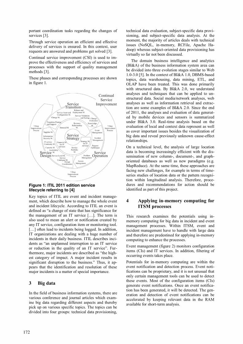
portant coordination tasks regarding the changes of

services [3].

Through service operation an efficient and effective

delivery of services is ensured. In this context, user

requests are answered and problems get solved [3].

Continual service improvement (CSI) is used to im-

prove the effectiveness and efficiency of services and

processes with the support of quality management

methods [3].

These phases and corresponding processes are shown

in figure 1.

Figure 1: ITIL 2011 edition service lifecycle referring to [4]

Key topics of ITIL are event and incident manage-

ment, which describe how to manage the whole event

and incident lifecycle. According to ITIL an event is

defined as “a change of state that has significance for

the management of an IT service […]. The term is also used to mean an alert or notification created by

any IT service, configuration item or monitoring tool.

[…] often lead to incidents being logged. In addition,

IT organizations are dealing with a huge number of

incidents in their daily business. ITIL describes inci-

dents as “an unplanned interruption to an IT service

or reduction in the quality of an IT service”. Fur-

thermore, major incidents are described as “the high-

est category of impact. A major incident results in

significant disruption to the business.” Thus, it ap-

pears that the identification and resolution of these major incidents is a matter of special importance.

3 Big data

In the field of business information systems, there are

various conference and journal articles which exam-

ine big data regarding different aspects and thereby

pick up on various specific topics. The topics can be

divided into four groups: technical data provisioning,

technical data evaluation, subject-specific data provi-

sioning, and subject-specific data analysis. At the

moment, the majority of articles deals with technical

issues (NoSQL, in-memory, RCFile, Apache Ha-

doop) whereas subject-oriented data provisioning has

virtually so far not been discussed.

The domain business intelligence and analytics (BI&A) of the business information system area can

be divided into three evolution stages similar to Web

1.0-3.0 [5]. In the context of BI&A 1.0, DBMS-based

topics, data warehousing, data mining, ETL, and

OLAP have been treated. This was done primarily

with structured data. By BI&A 2.0, we understand

analyses and techniques that can be applied to un-

structured data. Social media/network analyses, web

analyses as well as information retrieval and extrac-

tion are some examples of BI&A 2.0. Since the end

of 2011, the analyses and evaluation of data generat-

ed by mobile devices and sensors is summarized under BI&A 3.0. Real-time analysis based on the

evaluation of local and context data represent as well

as cover important issues besides the visualization of

big data and reveal previously unknown cause-effect

relationships.

On a technical level, the analysis of large location

data is becoming increasingly efficient with the dis-semination of new column-, document-, and graph-

oriented databases as well as new paradigms (e.g.

MapReduce). At the same time, these approaches are

facing new challenges, for example in terms of time-

series studies of location data or the pattern recogni-

tion within longitudinal analysis. Therefore, proce-

dures and recommendations for action should be

identified as part of this project.

4 Applying in-memory computing for

ITSM processes

This research examines the potentials using in-

memory computing for big data in incident and event

management processes. Within ITSM, event and

incident management have to handle with large data

and therefore are predestined for applying in-memory

computing to enhance the processes.

Event management (figure 2) monitors configuration

items (CIs) and IT services. In addition, filtering of

occurring events takes place.

Potentials for in-memory computing are within the

event notification and detection process. Event noti-

fications can be proprietary, and it is not unusual that

only certain management tools can be used to detect these events. Most of the configuration items (CIs)

generate event notifications. Once an event notifica-

tion has been generated, it will be detected. The gen-

eration and detection of event notifications can be

accelerated by keeping relevant data in the RAM

available for short-term analysis.

172

Second, in-memory computing can enhance the cor-

relation and filtering of first and second level events.

Event correlation is a technique for making sense of a

large number of events and detecting important

events in big data. Live analysis and identification of

correlations in real-time are enabled when data is

stored in the RAM.

Figure 2: ITIL 2011 edition event management process [3]

In incident management (figure 3), the lifecycle of all

incidents is managed. This process has the primary

goal of restoring IT services to business units as

quickly as possible. Important to understand, the

source of all the incidents is an incident classifica-tion. In-memory computing can be related to the

incident categorization. In order to gather incidents,

fields for category and subcategory exist, which

allow a classification. These categories can be used

by the system to create automatic assignment rules or

notifications. For instance, an important category for

incidents is their incident state. Based on this state

the service desk can track how much work has been

done, and identify the next process steps. While the

user enters categories, these can be compared and

possible categories can be recommended in real-time.

The organization can be affected differently by the

incidents. In order to handle the incidents a priority

based on the impact and urgency is defined. Enter-

prises can make use of this in order to manage a lot

of incidents and to minimize the incident impact on

the business. In large companies, prioritization of

incidents requires many computing resources due to

the large number of requests. With in-memory com-

puting, a dynamic prioritization can be realized. The

assignment of the priorities is based on dynamic

prioritization and live analysis of the data. In order to

identify viewpoints underlying a text span a so called

sentiment analysis can be used [6]. Given that users create incidents and comment on these, those com-

ments could be analyzed via sentiment analysis. The

real-time results could be used to help prioritize inci-

dents. Another possibility to make use of the fast data

processing of the in-memory database could be pat-

tern-matching to identify major incidents.

Figure 3: ITIL 2011 edition incident management process [3]

Figure 4 presents a high level view of the underlying

architecture. Within the project scope, we implement

monitoring nodes based on Nagios or Icinga in order

to monitor and control IT resources like databases,

web and ftp servers. Furthermore, these nodes ob-serve virtual machine (VM) hosts and single VMs. It

is necessary to distinguish between agent-based and

agentless monitoring; our nodes support both modes

of operation. These monitoring systems collect event

and sensor data from different sources in order to

transfer these via VPN to our HANA instance, where

a continual load into corresponding database tables

IMDB

IMDB

IMDB

1

2

3

4

IMDB

5

6

173

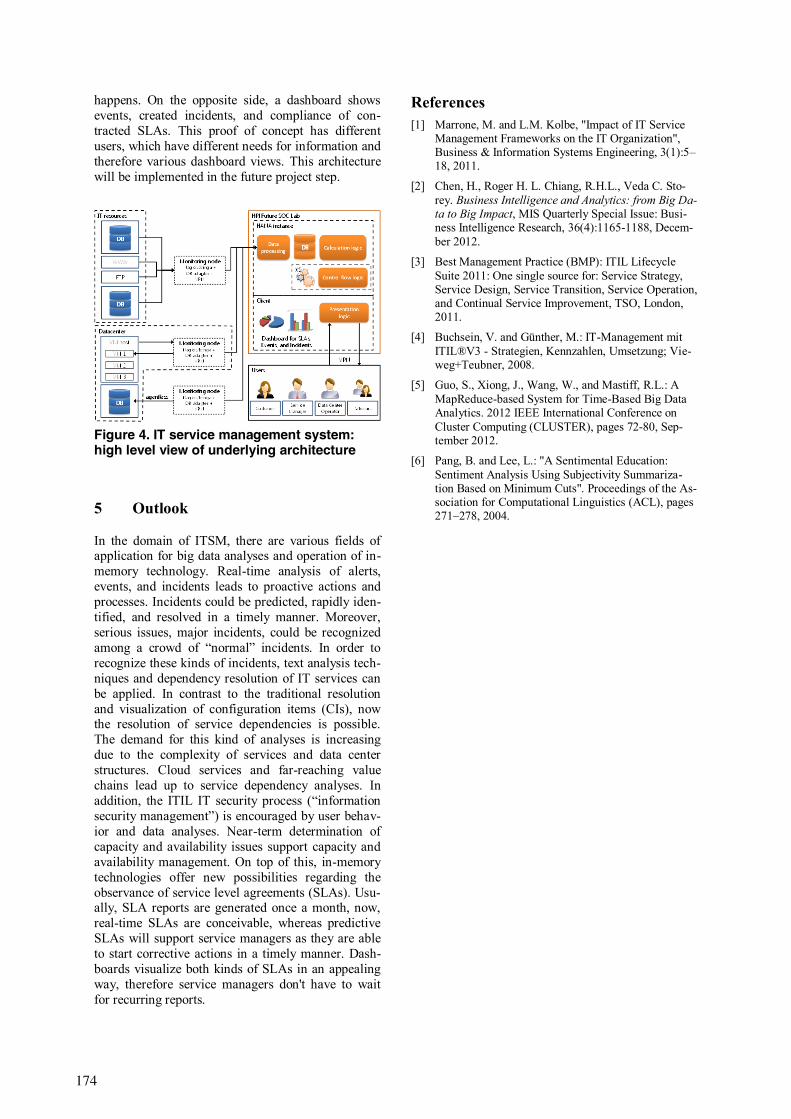
happens. On the opposite side, a dashboard shows

events, created incidents, and compliance of con-

tracted SLAs. This proof of concept has different

users, which have different needs for information and

therefore various dashboard views. This architecture

will be implemented in the future project step.

Figure 4. IT service management system: high level view of underlying architecture

5 Outlook

In the domain of ITSM, there are various fields of application for big data analyses and operation of in-

memory technology. Real-time analysis of alerts,

events, and incidents leads to proactive actions and

processes. Incidents could be predicted, rapidly iden-

tified, and resolved in a timely manner. Moreover,

serious issues, major incidents, could be recognized

among a crowd of “normal” incidents. In order to

recognize these kinds of incidents, text analysis tech-

niques and dependency resolution of IT services can

be applied. In contrast to the traditional resolution

and visualization of configuration items (CIs), now the resolution of service dependencies is possible.

The demand for this kind of analyses is increasing

due to the complexity of services and data center

structures. Cloud services and far-reaching value

chains lead up to service dependency analyses. In

addition, the ITIL IT security process (“information

security management”) is encouraged by user behav-

ior and data analyses. Near-term determination of

capacity and availability issues support capacity and

availability management. On top of this, in-memory

technologies offer new possibilities regarding the

observance of service level agreements (SLAs). Usu-ally, SLA reports are generated once a month, now,

real-time SLAs are conceivable, whereas predictive

SLAs will support service managers as they are able

to start corrective actions in a timely manner. Dash-

boards visualize both kinds of SLAs in an appealing

way, therefore service managers don't have to wait

for recurring reports.

References

[1] Marrone, M. and L.M. Kolbe, "Impact of IT Service Management Frameworks on the IT Organization", Business & Information Systems Engineering, 3(1):5–18, 2011.

[2] Chen, H., Roger H. L. Chiang, R.H.L., Veda C. Sto-

rey. Business Intelligence and Analytics: from Big Da-ta to Big Impact, MIS Quarterly Special Issue: Busi-ness Intelligence Research, 36(4):1165-1188, Decem-

ber 2012.

[3] Best Management Practice (BMP): ITIL Lifecycle

Suite 2011: One single source for: Service Strategy, Service Design, Service Transition, Service Operation, and Continual Service Improvement, TSO, London, 2011.

[4] Buchsein, V. and Günther, M.: IT-Management mit

ITIL®V3 - Strategien, Kennzahlen, Umsetzung; Vie-weg+Teubner, 2008.

[5] Guo, S., Xiong, J., Wang, W., and Mastiff, R.L.: A

MapReduce-based System for Time-Based Big Data Analytics. 2012 IEEE International Conference on

Cluster Computing (CLUSTER), pages 72-80, Sep-tember 2012.

[6] Pang, B. and Lee, L.: "A Sentimental Education:

Sentiment Analysis Using Subjectivity Summariza-tion Based on Minimum Cuts". Proceedings of the As-sociation for Computational Linguistics (ACL), pages 271–278, 2004.

174

Aktuelle Technische Berichte des Hasso-Plattner-Instituts

Band

ISBN

Titel

Autoren / Redaktion

87 978-3-86956-281-0

Cloud Security Mechanisms Christian Neuhaus, Andreas Polze (Hrsg.)

86 978-3-86956-280-3

Batch Regions Luise Pufahl, Andreas Meyer, Mathias Weske

85 978-3-86956-276-6

HPI Future SOC Lab: Proceedings 2012 Christoph Meinel, Andreas Polze, Gerhard Oswald, Rolf Strotmann, Ulrich Seibold, Bernhard Schulzki (Hrsg.)

84

978-3-86956-274-2

Anbieter von Cloud Speicherdiensten im Überblick

Christoph Meinel, Maxim Schnjakin, Tobias Metzke, Markus Freitag

83

978-3-86956-273-5

Proceedings of the 7th Ph.D. Retreat of the HPI Research School on Service-oriented Systems Engineering

Christoph Meinel, Hasso Plattner, Jürgen Döllner, Mathias Weske, Andreas Polze, Robert Hirschfeld, Felix Naumann, Holger Giese, Patrick Baudisch (Hrsg.)

82

978-3-86956-266-7

Extending a Java Virtual Machine to Dynamic Object-oriented Languages

Tobias Pape, Arian Treffer, Robert Hirschfeld

81 978-3-86956-265-0

Babelsberg: Specifying and Solving Constraints on Object Behavior

Tim Felgentreff, Alan Borning, Robert Hirschfeld

80 978-3-86956-264-3

openHPI: The MOOC Offer at Hasso Plattner Institute

Christoph Meinel, Christian Willems

79 978-3-86956-259-9

openHPI: Das MOOC-Angebot des Hasso-Plattner-Instituts

Christoph Meinel, Christian Willems

78 978-3-86956-258-2

Repairing Event Logs Using Stochastic Process Models

Andreas Rogge-Solti, Ronny S. Mans, Wil M. P. van der Aalst, Mathias Weske

77 978-3-86956-257-5

Business Process Architectures with Multiplicities: Transformation and Correctness

Rami-Habib Eid-Sabbagh, Marcin Hewelt, Mathias Weske

76 978-3-86956-256-8

Proceedings of the 6th Ph.D. Retreat of the HPI Research School on Service-oriented Systems Engineering

Hrsg. von den Professoren des HPI

75 978-3-86956-246-9

Modeling and Verifying Dynamic Evolving Service-Oriented Architectures

Holger Giese, Basil Becker

74 978-3-86956-245-2

Modeling and Enacting Complex Data Dependencies in Business Processes

Andreas Meyer, Luise Pufahl, Dirk Fahland, Mathias Weske

73 978-3-86956-241-4

Enriching Raw Events to Enable Process Intelligence

Nico Herzberg, Mathias Weske

72 978-3-86956-232-2

Explorative Authoring of ActiveWeb Content in a Mobile Environment

Conrad Calmez, Hubert Hesse, Benjamin Siegmund, Sebastian Stamm, Astrid Thomschke, Robert Hirschfeld, Dan Ingalls, Jens Lincke

71 978-3-86956-231-5

Vereinfachung der Entwicklung von Geschäftsanwendungen durch Konsolidierung von Programmier- konzepten und -technologien

Lenoi Berov, Johannes Henning, Toni Mattis, Patrick Rein, Robin Schreiber, Eric Seckler, Bastian Steinert, Robert Hirschfeld

Technische Berichte Nr. 88

des Hasso-Plattner-Instituts für Softwaresystemtechnik an der Universität Potsdam

HPI Future SOC Lab: Proceedings 2013Christoph Meinel, Andreas Polze, Gerhard Oswald, Rolf Strotmann, Ulrich Seibold, Bernhard Schulzki (Hrsg.)

ISBN 978-3-86956-282-7ISSN 1613-5652

HPI Future SOC Lab : Proceedings 2013 - Hasso-Plattner-Institut

Documents

Transcript of HPI Future SOC Lab : Proceedings 2013 - Hasso-Plattner-Institut