Policy Research Working Paper 9388

How Useful Is CPI Price Data for Spatial Price Adjustment in Poverty Measurement?

A Case from Ghana

Xiaomeng Chen Rose Mungai

Shohei NakamuraThomas Pearson

Ayago Esmubancha WambileNobuo Yoshida

Poverty and Equity Global Practice September 2020

Pub

lic D

iscl

osur

e A

utho

rized

Pub

lic D

iscl

osur

e A

utho

rized

Pub

lic D

iscl

osur

e A

utho

rized

Pub

lic D

iscl

osur

e A

utho

rized

Produced by the Research Support Team

Abstract

The Policy Research Working Paper Series disseminates the findings of work in progress to encourage the exchange of ideas about development issues. An objective of the series is to get the findings out quickly, even if the presentations are less than fully polished. The papers carry the names of the authors and should be cited accordingly. The findings, interpretations, and conclusions expressed in this paper are entirely those of the authors. They do not necessarily represent the views of the International Bank for Reconstruction and Development/World Bank and its affiliated organizations, or those of the Executive Directors of the World Bank or the governments they represent.

Policy Research Working Paper 9388

Measuring and comparing the levels of household welfare and poverty in a country require cost-of-living differences across regions to be properly adjusted. In measuring the spatial cost of living, the recent literature underscores the importance of detailed product quality information in the price data. Taking advantage of the price data availabil-ity in Ghana, this case study explores the Consumer Price Index price data as a source for spatial price measurement.

It applies the country product dummy method to the Con-sumer Price Index price data and compares the results with other methods based on different price data. The empirical analysis indicates a potential bias in estimating spatial prices stemming from the lack of product quality information and, therefore, suggests the potential usefulness of the Consumer Price Index price data for spatial price adjustment in poverty analysis in low- and middle-income countries.

This paper is a product of the Poverty and Equity Global Practice. It is part of a larger effort by the World Bank to provide open access to its research and make a contribution to development policy discussions around the world. Policy Research Working Papers are also posted on the Web at http://www.worldbank.org/prwp. The authors may be contacted at snakamura2@worldbank.org.

How Useful Is CPI Price Data for Spatial Price Adjustment in Poverty Measurement? A Case from Ghana

Xiaomeng Chen, World Bank

Rose Mungai, World Bank

Shohei Nakamura, World Bank1

Thomas Pearson, Boston University

Ayago Esmubancha Wambile, World Bank

Nobuo Yoshida, World Bank

JEL Classification: D12, E31, O15

Keywords: price indexes, household welfare, purchasing power parity, housing, Ghana

1 Corresponding author (snakamura2@worldbank.org). We would like to thank the Ghana Statistical Services (GSS) for allowing us to use the CPI price data for the analysis in this paper. We also thank Giovanni Vecchi and Nicola Amendola for their useful comments on the earlier version of the paper. The findings, interpretations, and conclusions expressed in this paper are entirely those of the authors. They do not necessarily represent the views of the International Bank for Reconstruction and Development (IBRD) or the World Bank and its affiliated organizations, or those of the Executive Directors of the World Bank or the governments they represent.

2

1. IntroductionThe basis for poverty and inequality analysis is household welfare, which is commonly measured by household consumption (Deaton and Zaidi 2002; Ravallion 2008).2 A key component of welfare measurement is price adjustment. To compare the welfare level of households over time and across regions, household consumption aggregates need to be adjusted by accounting for inflation (that is, temporal price adjustment) and cost-of-living differences across regions (that is, spatial price adjustment).3 Inappropriate adjustments of such price difference cause a bias in poverty estimation. Spatial price adjustment becomes particularly important when policy makers need to know not only who is poor but also where poverty is concentrated.4 Despite the importance of spatial price adjustment on welfare measurement for poverty and inequality analysis, its underpinning theory is not necessarily clear to guide the practice. Many low- and middle-income countries apply different methods, without a rigorous methodological foundation, often facing the limited availability of price data suitable for spatial price adjustment as the biggest challenge.5

The recently collected survey by the World Bank illustrates how the current practice of spatial price adjustment varies among Sub-Saharan African countries (Figure 1).6 In its internal process of developing a regional poverty database, the World Bank collected from 47 Sub-Saharan African countries information about the data sources and methods used for price adjustment. In terms of data sources (Panel A), about 40 percent of African countries rely on survey unit values, which is a proxy measure of prices calculated by dividing households’ expenditures by the purchased quantity for each good based on household budget or welfare surveys. While unit values might be useful in cases where price data are lacking, the problems related to unit values have been reported in several studies (Gibson and Kim 2019; McKelvey 2011). Another 26 percent of the countries use market price surveys, which are often collected in parallel to the official household budget or welfare surveys. A small number of countries use their Consumer Price Index (CPI) data for spatial price adjustment. The methodology of spatial price adjustment is more divided with countries applying different approaches (Panel B), including the Paasche index (25 percent), Laspeyres index (15 percent), Fisher index (13 percent), and so on.

2 Some countries rely on household income, instead of consumption, for poverty measurement (Ferreira et al. 2016). 3 ‘Region’ refers to subnational regions in this paper unless otherwise noted. 4 For example, as the cost of living in African cities is high relative to their income levels (Nakamura et al. 2019), urban poverty can be underestimated without adequate spatial price adjustment. 5 Some approaches to circumventing the data limitation include the Engel curve method (discussed in Appendix B of this paper) and price data collection from local experts (Gibson and Le 2018). 6 Africa refers to Sub-Saharan Africa in this paper unless otherwise mentioned.

3

Figure 1. Data and methods used for spatial price adjustment in Sub-Saharan African countries

(A) Data (B) Method

Source: Survey conducted by the World Bank. Note: PL = Poverty line.

Our study builds on, among others, recent research on spatial prices by Gibson, Le, and Kim (2017). In their study, Gibson, Le, and Kim compare the performance of different spatial price measurement approaches with the primary purpose to assess the reliability of a ‘no price data’ approach (that is, using the Engel curve-based method). The strength of their study is the use of Vietnam’s price survey that contains detailed product specification information, which gives them the gold standard to assess the performance of the Engel curve method. The analysis by Gibson, Le, and Kim (2017) suggests that the Engel curve method is unlikely to work for spatial price adjustment. We strongly agree with their argument that price data with detailed product quality information are necessary for spatial price adjustment for poverty measurement.

However, we do not necessarily insist on investment in the collection and expansion of market price surveys in low- and middle-income countries for poverty analysis. In this paper, we aim to examine the potential use of appropriate CPI raw price data for spatial price adjustment. While primarily designed and implemented for temporal price monitoring, the detailed product specification information in the CPI price data that is uniform across regions in a country could bring a great advantage in spatial price measurement. To examine the performance of such a CPI-based approach, we test different methods with different price data by focusing on Ghana. The methods we test include bilateral and multilateral price index approaches, the country product dummy (CPD) approach, and the spatial Engel curve approach. We apply these methods to the market price survey data collected in parallel to the official household budget survey (Ghana Living Standard Survey Round Seven [GLSS7]) and CPI raw price data.

Our analysis suggests that the CPD works reasonably when missing price observations exist across regions and detailed variety of product- or item-level information is available. Controlling for detailed quality information in the application of the CPD to the CPI data yields a convergence of regional price levels, due to the falling price level of Greater Accra relative to other regions (or conversely due to the increasing price levels of other regions relative to Greater Accra). This is because of the differences in the quality of goods and services available across the regions. Not controlling for these quality differences leads to a biased estimate of the price levels, which biases the price-level estimates of regions with higher-quality items (like Greater Accra) upward and those of regions with lower-quality items downward. While the CPI price data appear to be useful source data, this approach still needs to be complemented with other data sources, as housing prices in the CPI data are not directly useful for spatial price measures.

4

This paper is structured as follows. Section 2 reviews the theory and practice of spatial price adjustment to set out key issues to be addressed. Section 3 describes our methodology by explaining the empirical approach and data. Section 4 presents the results. Section 5 discusses the key findings and conclusions.

2. Spatial price adjustment: Theory and practice In this section, we first review the theory and practice of standard price index approaches. Then, we discuss methodological issues on non-food items, particularly housing, in measuring spatial differentials in costs of living. Finally, we introduce the CPD approach, which is the main approach in our empirical analysis.

2.1. How can standard price index approaches be improved given the limited data availability?

Choice of price index

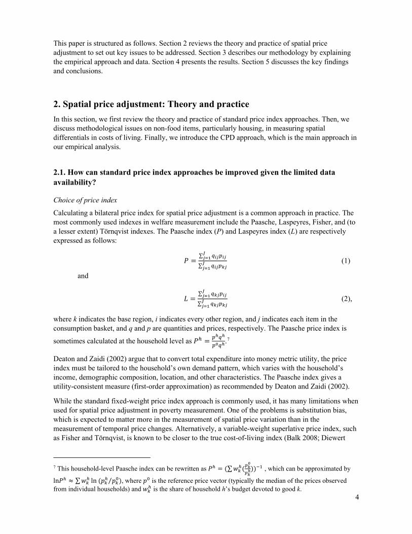
Calculating a bilateral price index for spatial price adjustment is a common approach in practice. The most commonly used indexes in welfare measurement include the Paasche, Laspeyres, Fisher, and (to a lesser extent) Törnqvist indexes. The Paasche index (P) and Laspeyres index (L) are respectively expressed as follows:

𝑃𝑃 =∑ 𝑞𝑞𝑖𝑖𝑖𝑖𝑝𝑝𝑖𝑖𝑖𝑖𝐽𝐽𝑖𝑖=1

∑ 𝑞𝑞𝑖𝑖𝑖𝑖𝑝𝑝𝑘𝑘𝑖𝑖𝐽𝐽𝑖𝑖=1

(1)

and

𝐿𝐿 =∑ 𝑞𝑞𝑘𝑘𝑖𝑖𝑝𝑝𝑖𝑖𝑖𝑖𝐽𝐽𝑖𝑖=1

∑ 𝑞𝑞𝑘𝑘𝑖𝑖𝑝𝑝𝑘𝑘𝑖𝑖𝐽𝐽𝑖𝑖=1

(2),

where k indicates the base region, i indicates every other region, and j indicates each item in the consumption basket, and q and p are quantities and prices, respectively. The Paasche price index is

sometimes calculated at the household level as 𝑃𝑃ℎ = 𝑝𝑝ℎ𝑞𝑞ℎ

𝑝𝑝0𝑞𝑞ℎ.7

Deaton and Zaidi (2002) argue that to convert total expenditure into money metric utility, the price index must be tailored to the household’s own demand pattern, which varies with the household’s income, demographic composition, location, and other characteristics. The Paasche index gives a utility-consistent measure (first-order approximation) as recommended by Deaton and Zaidi (2002).

While the standard fixed-weight price index approach is commonly used, it has many limitations when used for spatial price adjustment in poverty measurement. One of the problems is substitution bias, which is expected to matter more in the measurement of spatial price variation than in the measurement of temporal price changes. Alternatively, a variable-weight superlative price index, such as Fisher and Törnqvist, is known to be closer to the true cost-of-living index (Balk 2008; Diewert

7 This household-level Paasche index can be rewritten as 𝑃𝑃ℎ = (∑𝑤𝑤𝑘𝑘ℎ(𝑝𝑝𝑘𝑘

0

𝑝𝑝𝑘𝑘ℎ))−1 , which can be approximated by

ln𝑃𝑃ℎ ≈ ∑𝑤𝑤𝑘𝑘ℎ ln (𝑝𝑝𝑘𝑘ℎ 𝑝𝑝𝑘𝑘0⁄ ), where 𝑝𝑝0 is the reference price vector (typically the median of the prices observed from individual households) and 𝑤𝑤𝑘𝑘ℎ is the share of household h’s budget devoted to good k.

5

1976). Mathematically, the Fischer index (F) is a geometric average of the Laspeyres and Paasche indexes,

𝐹𝐹 = (𝐿𝐿 × 𝑃𝑃)1/2 (3),

and the Törnqvist index (T) is expressed as

𝑇𝑇 = exp [∑ �𝑤𝑤𝑘𝑘𝑖𝑖+𝑤𝑤𝑖𝑖𝑖𝑖

2�𝐽𝐽

𝑗𝑗=1 ln (𝑝𝑝𝑖𝑖𝑖𝑖𝑝𝑝𝑘𝑘𝑖𝑖

)] (4),

where wij is the average share that item j has in the consumption basket in region i.

The Laspeyres price index provides an upper limit on the true cost-of-living index (COLI) based on the standard of living in the initial price situation, while the Paasche price index provides a lower limit on the true COLI based on the standard of living in the given price situation. The Laspeyres index is relatively easy to calculate but sensitive to a substitution bias. The Fisher index is also utility-consistent (second-order approximation), bounded by the Paasche and Laspeyres indexes. However, the Fisher index is susceptible to income bias in case of non-homothetic preference. For the practicality of poverty and inequality analysis, the Fisher price index may work preferably, as the gap between the Paasche and Laspeyres price indexes tends to be wide in poor areas. However, the degree of the Paasche-Laspeyres spread is an empirical question.

Reference area and transitivity

Real household consumptions—that is, nominal consumptions deflated by a spatial price index—are compared to a poverty line to measure poverty. An important issue in a bilateral price index approach is the choice of reference area. Reference area in spatial price index needs to be the same as the location where the basket for poverty line is priced. For instance, if a poverty line is constructed based on the costs of basket items measured by the national prices (PLA), the consumption expenditure of household i in region r needs to be spatially deflated as

𝐸𝐸𝐸𝐸𝑃𝑃𝑖𝑖,𝑟𝑟 × 𝜋𝜋𝑟𝑟𝐴𝐴 = 𝐷𝐷𝐸𝐸𝐸𝐸𝑃𝑃𝑖𝑖,𝑟𝑟𝐴𝐴 (5),

where 𝜋𝜋𝑟𝑟𝐴𝐴 is a spatial price index that adjusts the consumption from the region r prices to the national prices (A). The price index 𝜋𝜋𝑟𝑟𝐴𝐴 can be considered as the ratio of price levels between region r and the national average A (𝑝𝑝𝐴𝐴 𝑝𝑝𝑟𝑟⁄ ). Then, the poverty status of household i can be identified by

𝐷𝐷𝐸𝐸𝐸𝐸𝑃𝑃𝑖𝑖,𝑟𝑟𝐴𝐴 ⋚ 𝑃𝑃𝐿𝐿𝐴𝐴 (6).

Similarly, if a poverty line is constructed based on the capital region prices (a), household consumption needs to be deflated by a spatial price index 𝜋𝜋𝑟𝑟𝑎𝑎, which indicates the price-level ratio between region r and region a.

It is important to note that changing the reference area ex post does not work if the spatial price index does not satisfy transitivity. In other words,

𝐸𝐸𝐸𝐸𝑃𝑃𝑖𝑖,𝑟𝑟 × 𝜋𝜋𝑟𝑟𝐴𝐴 × 𝜋𝜋𝐴𝐴𝑎𝑎 ≠ 𝐷𝐷𝐸𝐸𝐸𝐸𝑃𝑃𝑖𝑖,𝑟𝑟𝑎𝑎 (7).

Without transitivity satisfied in a spatial price index, the comparison of prices between two areas changes depending on the choice of the reference area. This is problematic in poverty measurement, as the choice of the reference area for the poverty line (and thus the reference area for the spatial price index) can alter poverty estimates. The Gini, Elteö, Köves, and Szulc (GEKS) procedure (Deaton and Heston 2010) is proposed to transform a bilateral index to a multilateral index. This approach is used

6

by the International Comparison Program (ICP) for the calculation of the international purchasing power parity (PPP) (World Bank 2015a, 2015b). The GEKS-Fisher index is calculated as follows:

𝐺𝐺𝐹𝐹𝑐𝑐 = (∏ 𝐹𝐹1𝑗𝑗𝐹𝐹𝑗𝑗𝑐𝑐𝑀𝑀𝑗𝑗=1 )1/𝑀𝑀 (8),

where F1j is the Fisher index for region j with region 1 as the reference area. This procedure is equivalent to taking a geometric mean of every possible combination of two regions. As discussed in Section 2.3, a multilateral price index can also be calculated by the CPD method.8

Choice of price data

While the choice of price index calculation methods matters, the quality and types of price data used for the calculation may be even more important. There are three types of data commonly available for spatial price adjustment. The first type of price data is the market price survey data that are typically collected in parallel with an official household budget survey. The second type of price data that can be potentially used for spatial price adjustment is the CPI price data. The third type of price data is unit values that can be calculated based on the consumption module of official household budget surveys. Gaddis (2016) nicely summarizes the general characteristics of these price data from a poverty analysis perspective as in Table 1. We encourage readers to refer to Gaddis (2016) for the discussion, and only highlight here some key factors particularly relevant to spatial price adjustment for poverty measurement below.9

8 The GEKS procedure can also be applied to the Törnqvist index (Caves, Christensen, and Diewert 1982; Balk 2008). Another common approach to calculate a multilateral index is the Geary-Khamis method, which is used by the Penn World Table (Feenstra, Inklaar, and Timmer 2015) and the regional price parities in the United States (Aten 2017). 9 Also see Chapter V of United Nations Statistics Division (2005). Aside from these commonly available price data, there are other types of price data, such as the price data collected for the PPP calculation under the ICP, scanner data collected by private companies, and price inventories of specific goods and services (agricultural products, housing, and so on). For example, recent research that takes advantage of scanner data demonstrates the impacts of quality (or item) variations on the costs of living across cities. Handbury and Weinstein (2015) use detailed barcode data to address heterogeneity bias (stemming from the comparison of different goods in different locations) and variety bias (stemming from not correcting for the fact that some goods are unavailable in some locations), finding that prices are lower (as opposed to higher) in larger cities in the United States. Feenstra, Xu, and Antoniades (2017) analyze China in a similar way and compare it to the United States. Other research with scanner data includes Handbury (2013), which constructs a spatial price index for different income levels (that is, non-homothetic) across the U.S. metropolitan areas. It finds that price levels for high-income households tend to be overestimated when a standard homothetic index is used.

7

Table 1. Stylized comparison of different price data sources Market price survey CPI price data Unit values Nationally representative

(+) (but a potentially large

number of missing values)

(−) (often only urban,

purposive sampling)

(+) (but potentially biased toward

purchasing households) Representative for survey strata

(+) (but a potentially large

number of missing values)

(−) (data collection delinked from household survey)

(+)

Sample size/number of observations

(−) (only few price

observations per item and cluster, missing values)

(−) (limited number of price observations per item)

(+) (large number of price

observations, especially for diary surveys)

Food and non-food coverage

(+) (often only few non-food

items)

(+) (−)

Precisely defined items

(+) (if enumerators are well

instructed)

(+) (typically well-trained

enumerators, every month)

(−) (generally not, especially

recall surveys with aggregated item list)

Direct measurement

(+) (+) (−) (computed as value divided by

quantity) Collection process

(−) (especially with nonresident

enumerators)

(−) (nonresident enumerators)

(+) (based on actual transactions)

Source: Gaddis (2016, 10) Although not many Sub-Saharan African countries have conducted market price surveys (see the list of countries in Table A1 in Appendix A), those price data are potentially a good source for spatial price adjustment. The market price surveys are often conducted in a sample of communities or market centers close to the enumeration areas (EAs) in parallel with official nationally representative budget surveys. Typically, only one price is recorded for each item in each community. A major disadvantage of market price surveys is the lack of detailed quality information. Without detailed information about item descriptions, it is not possible to compare prices of the same products across regions. Gibson, Le, and Kim (2017) explain that Vietnam’s price survey was carefully designed to record detailed information for each product.

As stated earlier, CPI price data are another potential source for spatial price adjustment. Unlike market price surveys, CPI price data exist in almost all countries (Berry et al. 2019). Since the CPI is an indicator of inflation, it does not indicate spatial differentials in costs of living.10 However, it is possible to calculate the spatial price index by using the CPI price data (not CPI values per se). The problem is that many countries collect price information only in urban areas (see Table A2 in Appendix A). Nevertheless, if the geographic coverage of the data is adequate, using the same price data for spatial and temporal price adjustment can be an efficient approach in terms of the data collection costs, and it could also enhance consistency between temporal and spatial price patterns.11 In addition, compared to market price surveys, a wide variety of food and non-food price information is collected in the CPI data, and the data collection is frequent (for example, monthly). A well-known issue is that the basket used for the calculation of the CPI is often skewed toward higher-income households. For

10 Some countries report regional CPIs. Such regional CPIs still do not indicate price differences across regions as they only indicate inflation in each region and do not utilize the data for determining spatial variations in cost of living across the regions. 11 Inconsistency in temporal and spatial price movements is not uncommon. Let us consider a spatial price index at year 0 (𝑆𝑆𝑃𝑃𝑆𝑆𝑡𝑡0) and year 1 (𝑆𝑆𝑃𝑃𝑆𝑆𝑡𝑡1). By applying the regional CPIs between t0 and t1 to 𝑆𝑆𝑃𝑃𝑆𝑆𝑡𝑡0, one can obtain another spatial price index (𝑆𝑆𝑃𝑃𝑆𝑆𝑡𝑡1∗ ). This index 𝑆𝑆𝑃𝑃𝑆𝑆𝑡𝑡1∗ often deviates from 𝑆𝑆𝑃𝑃𝑆𝑆𝑡𝑡1.

8

spatial price adjustment for poverty analysis, it may be useful to exclude items that are not relevant to low-income households.12

A few but growing number of countries have either officially reported or published as experiments subnational PPPs calculated based on the CPI price data. Those examples include the United States (Aten 2017), the United Kingdom (Office for National Statistics 2018), Germany (Weinand and von Auer 2019), and Italy (Biggeri and Tiziana 2014; Laureti and Rao 2018). An example from a developing country is Dikhanov, Palanyandy, and Capilit (2011) for the Philippines.

Finally, when price data (based on price surveys) are not available, unit values are often used as a proxy for price. As shown in Figure 1, about 40 percent of African countries currently rely on unit values for spatial price adjustment for their official poverty measurement. Unit values have advantages in several aspects, including their availability and geographic coverage. Nevertheless, the limited information about product quality and non-food goods and services is clearly a serious drawback for spatial price adjustment. An example is a substitution bias due to unobserved quality differences in unit values. Since Deaton (1986) established the use of unit values several decades ago, various adjustment methods have been devised to address concerns about the reliability of unit values (Gibson, n.d.). Recent research, however, has emphasized limitations in the use of unit values as a proxy for price data (Gibson and Kim 2019; McKelvey 2011). Thus, it would be better to avoid resorting to unit values for spatial price adjustment unless other price data are not available. In this paper, we focus on market price surveys and the CPI price data.

2.2. How should non-food items (particularly housing) be treated in measuring spatial differentials in the cost of living?

Treatment of non-food prices

As people become richer, they tend to spend a lesser portion of their budget on food expenditures. This empirical association between income and food budget share is known as Engel’s law. A similar pattern is observed even at a cross-country comparison, as the average food budget share is higher in low- and middle-income countries (Figure 2). In many African countries, people typically spend more than half of their budget on food expenditures. However, this does not justify the construction of a spatial deflator for poverty measurement solely on food prices. As economies develop, non-tradable non-food items tend to account for a large portion of price dispersion across regions (for example, the Balassa-Samuelson effect), highlighting the importance of measuring those prices.

12 For example, Rwanda uses CPI price data to calculate a COLI for poverty measurement (National Institute of Statistics of Rwanda 2016). In the calculation of the COLI, it uses only items that are included in the basket used for poverty line construction. Another interesting study is Dikhanov et al. (2017), which calculates the PPP by focusing on items relevant for low-income households in Africa.

9

Figure 2. Engel curves of world countries

Source: Ravallion and Chen (2015).

A sound spatial price adjustment requires price information about a variety of non-food goods and services. For example, the ICP collects for the PPP calculation the following non-food price information at the aggregated category level: clothing and footwear; housing, water, electricity, gas, and other fuels; furnishing, household equipment, and routine maintenance of the house; health; transport; communication; recreation and culture; education; restaurants and hotels; and other miscellaneous goods and services (World Bank 2015b). However, it is challenging to properly compare prices of non-food items across regions due to the heterogeneity of the items and lack of information about the quality difference particularly for the market price survey data and the survey unit values. Calculating unit values of non-food items is particularly difficult, with a few exceptions, such as items in the fuel category that are sometimes less susceptible to quality bias.

Treatment of housing

Among a handful of developed countries that report subnational PPP, their approaches to capturing housing prices vary. While the regional price parities are calculated based on the CPI price data in the United States (Aten 2017), housing rent information is retrieved from another source: the American Community Survey (ACS). Similarly, Weinand and von Auer’s (2019) calculation of regional PPP for Germany based on the CPI price data relies on another database for housing prices, collected by a federal agency from advertisements in newspapers and the Internet. These methodological choices and differences in source data reflect the difficulty of relying on the CPI price data for housing prices. In the case of the CPI-based subnational PPP in the United Kingdom (Office for National Statistics 2018), housing prices are not considered at all. Unlike subnational PPP work in the developed countries, a reliable housing price database (which includes low-quality and/or informal housing and rural housing) rarely exists in developing countries. Thus, Living Standards Measurement Survey (LSMS) type of household surveys are often used for housing rent information. For instance, Gibson, Le, and Kim (2017) use self-reported dwelling values in Vietnam’s household survey.

Conceptually, there are different treatments of housing in spatial price measurement, such as the Acquisitions approach, Payments approach, and Uses approach. Melser and Hill (2007) provide a useful review of them. Among these is the Uses approach recommended by Melser and Hill (2007) for welfare measurement, as the cost-of-living index measures the change in the cost of maintaining a given standard of living or level of utility (CPI Manual 2004). The rental equivalence method is a common tool adopted in the Uses approach (CPI Manual 2004; Diewert 2003, 2009).

While we agree with the use of the rental equivalence approach, there are two key methodological decisions to be made in incorporating housing prices in the spatial price index calculation. The first

10

question is how to consider housing costs faced by households that pay no rent and the housing price level of a region where a large portion of residents are with such rent-free accommodations. In practice, either actually paid or imputed housing rents or (self-reported) housing values are used to incorporate housing costs in measuring costs of living across space. While housing rents are often imputed for owner-occupied housing units, rental housing markets need to be reasonably large for such imputation. Rent imputation can also be useful for housing units with nonmarket rate rents, such as public housing. More relevant in the context of the developing world is informal housing. Residents in informal settlements sometimes pay no rents or negligible rents. When constructing a consumption aggregate for welfare measurement, it may be better to use imputed rents for those residents. If the actual rent values do not reflect market values of their housing units, the welfare levels of the residents could be underestimated.13 By contrast, in case of constructing a spatial price index, it may not be necessary to impute rents for informal settlements. When measuring the price level of a region in which a majority of residents are in rent-free accommodations, imputing their rents could result in an overestimation of prices.

The second question is whether to adjust for housing quality differences in spatial price adjustment for welfare and poverty measurement. There are several ways to calculate a housing price index across space. A simple way is to take the average (or median) of housing rents at some geographic level. For example, Moretti (2013) averages gross housing rents (that is, housing rents plus utilities) of two- or three-bedroom apartments in each U.S. metropolitan area. An alternative and common approach is to estimate a hedonic regression model:

𝑦𝑦𝑖𝑖𝑗𝑗 = 𝛼𝛼 + 𝛽𝛽𝐸𝐸𝑖𝑖𝑗𝑗 + 𝛾𝛾𝑗𝑗𝐷𝐷𝑗𝑗 + 𝜀𝜀𝑖𝑖𝑗𝑗 (9),

where y is housing rent (or the natural logarithm of housing rent) of housing unit i in region j, X is a vector of housing characteristics, and D is a location dummy. The coefficients for the location dummy indicate price levels (relative to the reference location) after controlling for observed difference in housing quality. This type of hedonic approach is commonly used to calculate a housing price index (Moulton 1995). However, it may not be appropriate to control for housing quality in measuring spatial price differentials in the cost of living.

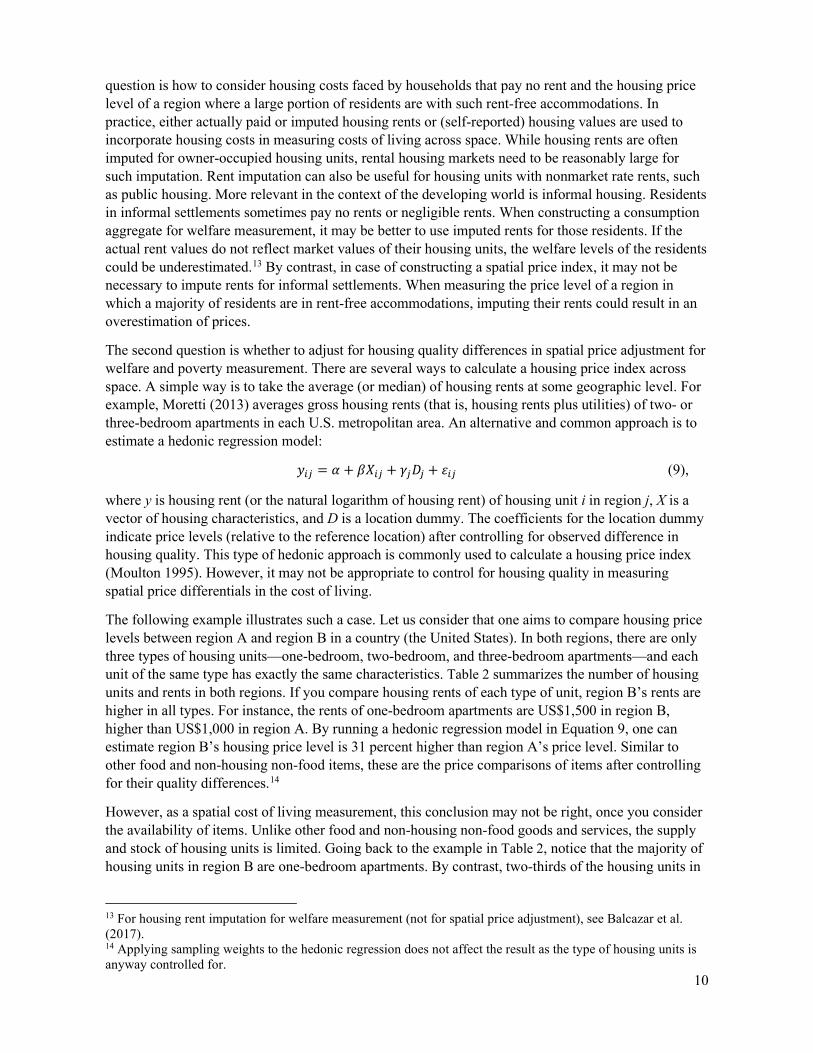
The following example illustrates such a case. Let us consider that one aims to compare housing price levels between region A and region B in a country (the United States). In both regions, there are only three types of housing units—one-bedroom, two-bedroom, and three-bedroom apartments—and each unit of the same type has exactly the same characteristics. Table 2 summarizes the number of housing units and rents in both regions. If you compare housing rents of each type of unit, region B’s rents are higher in all types. For instance, the rents of one-bedroom apartments are US$1,500 in region B, higher than US$1,000 in region A. By running a hedonic regression model in Equation 9, one can estimate region B’s housing price level is 31 percent higher than region A’s price level. Similar to other food and non-housing non-food items, these are the price comparisons of items after controlling for their quality differences.14

However, as a spatial cost of living measurement, this conclusion may not be right, once you consider the availability of items. Unlike other food and non-housing non-food goods and services, the supply and stock of housing units is limited. Going back to the example in Table 2, notice that the majority of housing units in region B are one-bedroom apartments. By contrast, two-thirds of the housing units in

13 For housing rent imputation for welfare measurement (not for spatial price adjustment), see Balcazar et al. (2017). 14 Applying sampling weights to the hedonic regression does not affect the result as the type of housing units is anyway controlled for.

11

region A are expensive three-bedroom apartments. Both mean and median values of housing rents are indeed lower in region B than in region A. If one assumes housing stock is unlimited like other goods, then the hedonic regression approach may work. Otherwise, it would be better not to control for quality differences in measuring housing costs in spatial price adjustment. This statement sounds contradictory to our emphasis on the detailed product specification information in other goods and services. This is because housing is a unique case in which its supply and stock are limited in a given market.

Table 2. A simple example of housing price index Region A Region B Units Rent ($) Units Rent ($) One-bedroom 10 1,000 40 1,500 Two-bedroom 10 3,000 10 4,000 Three-bedroom 40 5,000 10 6,000 Price index based on hedonic regression 60 1,000 60 1,310 Mean rent 60 4,000 60 2,670 Median rent 60 5,000 60 1,500

Note: Number of housing units is expressed in thousands.

2.3. What are the alternatives to the standard price index approaches? How are they better?

With the aforementioned methodological discussion in mind, we introduce here the CPD approach based on the CPI price data. Before getting there, however, we briefly touch upon another approach in spatial adjustment, which calculates a spatial price index based on multiple poverty lines. Multiple poverty line approach

An alternative and less common approach to measuring poverty is to construct regional poverty lines that reflect regional differences in the costs and needs to achieve the threshold utility. Poverty is measured by comparing each household’s nominal (that is, not spatially deflated) consumption aggregate to the region’s poverty line.15 An advantage of this approach is that regional price levels of non-food items can be flexibly calculated. Since non-food allowance is typically determined based on the expenditure shares of households around food poverty lines (Ravallion and Bidani 1994), price data for non-food items is not required. When analyzing inequality or comparing household welfare across regions, one can construct a spatial price index by taking ratios of regional poverty lines. Due to the complexity of the methodology, however, regional poverty lines are used in only a few countries. The analysis of this approach is outside the scope of this paper.

CPD approach

A challenge in spatial comparison of prices is that some items are not sold in some regions, and therefore, those prices are missing when calculating a price index. The CPD approach was originally developed to handle such missing values in price observations across regions (Rao 2004, 2005; Summers 1973).

15 Examples include Ravallion and Lokshin (2006) for the Russian Federation; Jolliffe, Datt, and Sharma (2004) for the Arab Republic of Egypt, and Marivoet and de Herdt (2015) for the Democratic Republic of Congo.

12

The CPD model is formulated as follows. The price of item i in region j (𝑝𝑝𝑖𝑖𝑗𝑗) is the product of the price level of item i relative to other items (𝜋𝜋𝑖𝑖), the price level (or the PPP) of region j with respect to other regions (𝜂𝜂𝑗𝑗), and a random disturbance term (𝑢𝑢𝑖𝑖𝑗𝑗).

𝑝𝑝𝑖𝑖𝑗𝑗 = 𝜋𝜋𝑖𝑖 ∙ 𝜂𝜂𝑗𝑗 ∙ 𝑢𝑢𝑖𝑖𝑗𝑗 (10),

which can be rewritten as follows:

ln 𝑝𝑝𝑖𝑖𝑗𝑗 = ln 𝜋𝜋𝑖𝑖 + ln 𝜂𝜂𝑗𝑗 + ln 𝑢𝑢𝑖𝑖𝑗𝑗 (11)

This model can be estimated as the following ordinary least squares (OLS) regression model.

ln𝑝𝑝𝑖𝑖𝑗𝑗 = ∑ 𝛼𝛼𝑖𝑖𝐷𝐷𝑖𝑖𝑁𝑁𝑖𝑖=2 + ∑ 𝛽𝛽𝑗𝑗𝐷𝐷𝑗𝑗𝑁𝑁

𝑗𝑗=2 + 𝜀𝜀𝑖𝑖𝑗𝑗 (12),

where 𝛼𝛼𝑖𝑖 = ln𝜋𝜋𝑖𝑖, 𝛽𝛽𝑗𝑗 = ln𝜂𝜂𝑗𝑗, and Di and Dj are item and region dummy variables. The price level of region j is calculated as 𝜂𝜂𝑗𝑗 = exp (�̂�𝛽𝑗𝑗). A weighted version of the CPD model (WCPD) is estimated as a weighted least squares regression model. Gibson, Le, and Kim (2017) propose two types of weights 𝑤𝑤𝑖𝑖𝑗𝑗. With 𝑠𝑠𝑖𝑖𝑗𝑗 as the average budget share of item i in region j, variable weights, (𝑠𝑠𝑖𝑖𝑗𝑗 + 𝑠𝑠𝑖𝑖0)/2, allow for substitution, while fixed weights, 𝑠𝑠𝑖𝑖0, do not depend on homothetic preferences. The spatial price index based on variable weights and fixed weights is calculated as follows:

𝜌𝜌𝑗𝑗𝑣𝑣𝑤𝑤 = [∑ (𝑠𝑠𝑖𝑖𝑖𝑖+𝑠𝑠𝑖𝑖02

)ln (𝑝𝑝𝑖𝑖𝑖𝑖𝑝𝑝𝑖𝑖0

)𝑁𝑁𝑖𝑖=1 ] (13)

and

𝜌𝜌𝑗𝑗𝑓𝑓𝑤𝑤 = [∑ (𝑠𝑠𝑖𝑖0)ln (𝑝𝑝𝑖𝑖𝑖𝑖

𝑝𝑝𝑖𝑖0)𝑁𝑁

𝑖𝑖=1 ] (14)

Gibson, Le, and Kim (2017) propose fixed-weights and variable-weights approaches.16 When the CPD is applied to individual price quotes, additional controls, such as outlet types and urban/rural, can be included (Hill and Syed 2015).

The CPD method has several advantages. First, the CPD method can be applied to the price data with missing observations across regions. In calculation of a standard price index (for example, Fisher price index), one has to drop items whose prices are not recorded in some regions. The CPD can be still applied to such data without dropping those items. Second, subnational PPPs calculated from the CPD model 𝜂𝜂𝑗𝑗 = exp��̂�𝛽𝑗𝑗� satisfy transitivity (Rao 2005). Therefore, one can directly calculate a multilateral price index without relying on the GEKS procedure. Finally, as the CPD is a regression model, it is possible to obtain standard errors for the price index values. This stochastic approach is, however, not backed up by the economic theory.

The CPD approach has been used in the research and practices on spatial price measurement. The CPD approach was originally used by Summers (1973) to calculate the international PPPs. Recent applications for the calculations of subnational price measurement include Laureti and Rao (2018); Weinand and von Auer (2019); Gibson, Le, and Kim (2017); and Dikhanov, Palanyandy, and Capilit (2011). In practice, the CPD can be used to either aggregate the price data from the variety level to the item (or basic heading) level or directly calculate a price index, which satisfies transitivity. The ICP applies the CPD method for the aggregation to the basic heading level in its PPP calculation (World Bank 2015b).

16 The variable-weights approach is equivalent to the Törnqvist index as shown in Diewert 2005.

13

In the next section, we explain our methodology to examine the issues described above based on a case study of Ghana.

3. Methodology

3.1. Ghana context and price data

Ghana context

The official poverty level in Ghana is measured based on the nationally representative household budget survey (Ghana Living Standard Survey [GLSS]). GLSS7 covered 14,009 households in 1,000 EAs and was conducted over a 12-month period between October 2016 and September 2017 (GSS 2018).17 The sampling was designed so that the survey gives information representative of urban and rural areas and across the 10 regions. Household-level consumption aggregates include both food (including auto-consumption) and non-food (including imputed housing rents) consumption. Further, consumption aggregates are converted to per adult equivalent annual consumption for poverty measurement to reflect differences in household size and composition and differences in calorie requirements of household members.

Consumption aggregates are deflated both temporally and spatially. The temporal deflation adjusts the differences in the timing of data collection between October 2016 and September 2017. Monthly regional CPI indexes are used for the within-survey-months temporal deflation. The spatial deflation on the other hand adjusts for the differences in the cost of living across the 10 regions based on the official regional CPI values. The reference region of the spatial deflation is Greater Accra (January 2017). Ghana measures poverty based on the single poverty line approach, that is, there is only one poverty line (GSS 2018). Spatial cost of living differentials are adjusted at the consumption side (as opposed to the multiple poverty line approach where poverty lines account for spatial price differences). The poverty line value is GH₵1,760.8 per adult equivalent per year, which was deflated by using a mixed deflator based on CPI raw price data and survey weights from the original poverty line of January 2013 (GH₵1,314). The official poverty headcount ratio in Ghana in 2016/17 is 23.4 percent, where urban and rural poverty is 7.8 percent and 39.5 percent, respectively (GSS 2018). Gini coefficients are 41.6 at the national level, 36.5 in urban areas, and 40.5 in rural areas. Price data

For this study, the main price data sets we use are the market price survey data from GLSS7 and CPI price data.18 The market price survey was collected from 398 clusters (or EAs in the GLSS7 data collection), of which 209 clusters are located in urban areas and 189 clusters are located in rural areas (Table 3). Those clusters cover 174 districts in all the 10 regions of the country. Out of 109 food items found in the GLSS7 consumption module, the market price survey has price information for 96 of them. The CPI price data are regularly collected from 44 markets, covering all the 10 regions of the

17 The previous rounds of GLSS surveys were conducted in 1987/88, 1988/89, 1991/92, 1998/99, 2005/06, and 2012/13. 18 Survey unit values cannot be calculated based on the GLSS7 consumption module due to the prevalence of nonstandard units and lack of conversion factors.

14

country.19 Table C1 and Table C2 in Appendix C show detailed information about the list of goods and services considered for our study and associated budget shares (calculated based on GLSS7).

Table 3. Price data in Ghana GLSS7 consumption module Market price survey CPI price data Geographic coverage

• 1,000 clusters • 214 districts • 10 regions

• 398 clusters (urban 209; rural 189)

• 174 districts • 10 regions

• 44 markets • 10 regions

Food items 109 items 96 items in GLSS7 consumption module matched

67 items in GLSS7 consumption module matched

Non-food items Paid rents and imputed rents available with quality information

Limited housing information

Limited housing information

We compare price distributions of major food items in the market price survey and CPI price data. Figure 3 shows price distributions of the following food items: smoked herring and salmon, bread, smoked fish, maize (ground or dough), imported rice, fresh tomatoes, water, yam and water yam, local rice, and large onions.20 Median price values between the market price survey and the CPI database are overall similar with smoked fish and water as exceptions.

19 Prices of about 307 items are regularly collected using the 2018 Classification of Individual Consumption According to Purpose (COICOP). 20 For each item, observations are treated as outliers and removed if their log prices are above or below 2.5 standard deviations.

15

Figure 3. Comparison of prices in the GLSS and CPI price data

Source: Authors’ calculations based on the GLSS7 market price survey and the CPI price database. Note: Outside values are not shown.

For housing information, we rely on GLSS7. Table 4 lists housing rent information in GLSS7. In urban areas, 2,138 out of 3,880 households (35.5 percent) paid rents. In rural areas, only 9 percent of households pay rents, which clearly demonstrates the challenge of imputing rents based on such a small size of rental markets in rural areas.

Table 4. Housing rent information in GLSS7 Urban Rural Observed Not observed Observed Not observed Western 213 316 86 716 Central 215 406 144 553 Greater Accra 505 766 34 93 Volta 171 302 82 812 Eastern 197 392 91 715 Ashanti 425 617 112 581 Brong Ahafo 208 365 95 650 Northern 76 354 28 951 Upper East 63 216 19 1,073 Upper West 65 146 31 1,125 Total 2,138 3,880 722 7,269

Source: Authors’ calculations based on GLSS7. Note: Sampling weights are not applied. ‘Observed’ indicates the number of households that actually paid rents (including subsidized rents); ‘Not observed’ indicates the number of households that did not pay any rent.

16

3.2. Empirical approach The main question we attempt to address is whether, and how, the CPI price data is useful for spatial price adjustment in poverty measurement, given the importance of detailed product quality information. To empirically examine it in this case study of Ghana, we compare the results of various spatial price measurement methods. The main methods we test are (a) the bilateral/multilateral price index approach, (b) the CPD approach, and (c) the Engel curve approach. The main data sets include (a) the market price survey data collected in parallel to the household budget survey and (b) CPI raw price data. The Engel approach requires no price data.

Price index approach

We first calculate several bilateral price indexes, such as the Paasche index (Equation 1), Laspeyres index (Equation 2), and Fisher index (Equation 3), as described in Section 2.1, and compare the spatial price patterns indicated based on each approach. We also compare these results with those based on a multilateral price index (GEKS-Fisher index in Equation 8) to assess how transitivity (or lack thereof) influences the results. CPD approach

We examine the two types of CPD methods. The first approach is to use the weighted CPD (Equation 12) to calculate the multilateral price index by applying it to the item-level price data for which budget share information is available as the weight. While we apply both variable weights (Equation 13) and fixed weights (Equation 14), following Gibson, Le, and Kim (2017), we report only the results based on variable weights, as no substantial difference is found in the results depending on the weights.21 The result of this approach is compared with a multilateral price index calculated by a GEKS-Fisher index method. Of particular interest in this comparison is how handling missing values by the CPD approach affects the spatial price measures.

Non-food prices

As discussed in Section 2.2, the treatment of non-food items, particularly housing, is a vital issue in the calculation of spatial price indexes. The combination of using the CPD method and the CPI price data allows us to include many non-food items without losing quality information in the price data. In the approach, we compare the spatial patterns of (a) the food price index and (b) the food plus non-food price index. In addition, we test the sensitivity of price measures to the omission of quality information (for both food and non-food items) by comparing the results with or without variety-level quality information in price observations.

For housing, we examine different approaches in the following aspects. First, we explore the influence of controlling for quality differences in housing across regions. We compare the results of spatial price measures based on the median values (that is, no control of quality) or hedonic regression (that is, with control of quality). Second, we also compare the results based on a price index that uses actually paid rents (that is, only rental units) and imputed rents (that is, owner-occupied and/or rent-free units included). The combination of these two aspects results in the following four housing approaches:

• Median paid rent approach takes a median value of paid rents in each region. • Median imputed rent approach takes a median value of paid and imputed rents in each region. • Hedonic paid rent approach estimates a hedonic regression model on paid rents in which

coefficients for the regional dummy indicate housing price levels.

21 Results based on fixed weights are available upon request.

17

• Hedonic imputed rent approach estimates a hedonic regression model on paid and imputed rents in which coefficients for the regional dummy indicate housing price levels.

Engel curve approach

Another approach to measuring spatial prices and welfare is the Engel curve method. We report the methodology and results in Appendix B. In line with Gibson, Le, and Kim (2017), our empirical analysis implies that the Engel curve approach is not suitable for spatial price measurement.

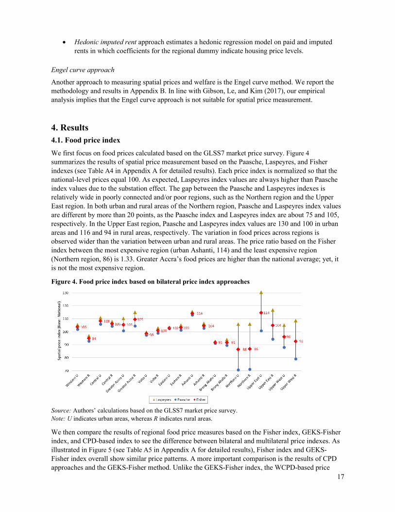
4. Results 4.1. Food price index We first focus on food prices calculated based on the GLSS7 market price survey. Figure 4 summarizes the results of spatial price measurement based on the Paasche, Laspeyres, and Fisher indexes (see Table A4 in Appendix A for detailed results). Each price index is normalized so that the national-level prices equal 100. As expected, Laspeyres index values are always higher than Paasche index values due to the substation effect. The gap between the Paasche and Laspeyres indexes is relatively wide in poorly connected and/or poor regions, such as the Northern region and the Upper East region. In both urban and rural areas of the Northern region, Paasche and Laspeyres index values are different by more than 20 points, as the Paasche index and Laspeyres index are about 75 and 105, respectively. In the Upper East region, Paasche and Laspeyres index values are 130 and 100 in urban areas and 116 and 94 in rural areas, respectively. The variation in food prices across regions is observed wider than the variation between urban and rural areas. The price ratio based on the Fisher index between the most expensive region (urban Ashanti, 114) and the least expensive region (Northern region, 86) is 1.33. Greater Accra’s food prices are higher than the national average; yet, it is not the most expensive region.

Figure 4. Food price index based on bilateral price index approaches

Source: Authors’ calculations based on the GLSS7 market price survey. Note: U indicates urban areas, whereas R indicates rural areas.

We then compare the results of regional food price measures based on the Fisher index, GEKS-Fisher index, and CPD-based index to see the difference between bilateral and multilateral price indexes. As illustrated in Figure 5 (see Table A5 in Appendix A for detailed results), Fisher index and GEKS-Fisher index overall show similar price patterns. A more important comparison is the results of CPD approaches and the GEKS-Fisher method. Unlike the GEKS-Fisher index, the WCPD-based price

18

indexes estimate the Greater Accra region as the most expensive (17 percent more expensive than the national average). Another profound difference between the WCPD results and the GEKS-Fisher price index is found in the Upper East region. The GEKS-Fisher price index indicates the Upper East as the most expensive region in Ghana in terms of food prices. The region’s price level, however, becomes moderate in the WCPD results—even lower than the national level.

Figure 5. Food price index based on multilateral price index approaches

Source: Authors’ calculations based on the GLSS7 market price survey. Note: Variable weights are applied to the CPD regression.

Next, we examine how the choice of data, instead of the choice of index calculation methods, influences the estimation of spatial price patterns (Figure 6). We compare the regional price indexes calculated by the WCPD method (based on variable weights) using the market price survey data and the CPI database. We first exploit only item-level price information in the CPI price database. The regional price index values based on the market price survey and the CPI price data are overall similar, as the Greater Accra and North regions are the most and least expensive regions, respectively. However, CPI-based values are substantially higher than GLSS-based values in the Upper West region and (to a lesser extent) the Volta region. For the Upper West region, CPI- and GLSS-based index values are 102.8 and 92.4, respectively.

Figure 6 shows another important CPI-based price index that is calculated based on a WCPD regression with a control of variety information (see Table A5 for detailed results). The comparison of regional price index values based on the CPI-based WCPD approach with and without control for variety information points to the impact of potential bias due to the lack of product quality information. Regional price dispersion is estimated to be smaller when variety-level information is controlled for in the WCPD regression. While remaining as the most expensive region, Greater Accra’s price level falls considerably. This is probably because Greater Accra was originally estimated to be expensive due to the prevalence of high-quality goods and services.

19

Figure 6. Food price index based on CPD approaches (GLSS and CPI price data)

Source: Authors’ calculations based on the GLSS 7 market price survey and CPI price data. Note: Variable weights are applied to the CPD regression.

4.2. Food plus non-food price index We then calculate spatial price indexes based on both food plus non-food prices in the CPI price data. Figure 7 summarizes the results, as well as the food only price index for comparison (see Table A6 in Appendix A for detailed results). Similar to the observations above on food prices, the inclusion of variety-level product information reduces the overall variation in spatial price levels. For instance, the price index for Greater Accra decreases from 111 based on the item-level price data to 106 based on the variety-level price data. It is also interesting to observe that adding non-food prices makes the Upper West region—which is the poorest region in Ghana—the most expensive region. There are several potential reasons for the relatively high price level in the Upper West region. It could be high transport costs that raise the prices of goods and services in the region. A more methodological reason may be the prevalence of low-quality products in the region.

Figure 7. Food + non-food index based on CPD approaches (CPI price data)

Source: Authors’ calculations based on the CPI price data. Note: Variable weights are applied to the CPD regression.

20

4.3. Food plus non-food and housing price index Adding housing prices to spatial price index calculations can meaningfully change the estimated spatial pattern of prices. Before presenting the results of such a total price index, however, we look at housing price indexes per se. As explained in Section 3.1, we employ several approaches to analyze housing prices. Figure 8 summarizes the results (see Table A7 in Appendix A for detailed results). Table A8 in Appendix A reports the results of hedonic regression estimations. In Figure 8, we normalize the price index so that the value in Greater Accra is 100 for the presentation purpose. Housing prices in Greater Accra are by far the most expensive, as all the other regions have index values less than 60, regardless of the choice of housing approaches. Nonetheless, it is observed that the hedonic imputed rent approach yields upper-bound estimates, while the median paid rent approach gives lower-bound estimates. This is not surprising, as the hedonic imputed rent approach assigns imputed rents to rent-free accommodations and controls for quality differences across units. By contrast, the median paid rent approach does not control for quality differences.

Figure 8. Housing price indexes

Source: Authors’ calculations based on the GLSS7 data. Note: Median paid rent approach takes a median value of paid rents in each region; Median imputed rent approach takes a median value of paid and imputed rents in each region; Hedonic paid rent approach estimates a hedonic regression model on paid rents in which coefficients for the regional dummy indicate housing price levels; and Hedonic imputed rent approach estimates a hedonic regression model on paid and imputed rents in which coefficients for the regional dummy indicate housing price levels.

Finally, we calculate regional price indexes by incorporating food prices, non-food prices, and housing prices. In this calculation, we use the CPI price data for food and non-food goods and services and the GLSS household survey data for housing prices. Figure 9 presents the results (see Table A6 and Table A7 in Appendix A for detailed results). Once housing costs are properly considered, the total price indexes indicate that Greater Accra is the most expensive region in the country—14 percent more expensive than the national average. Ashanti and Upper West also remain relatively expensive regions. The modest change in Greater Accra’s price level—despite the high housing costs—is due to the small expenditure share devoted to housing costs.22 In any event, household expenditures for housing in a

22 For instance, nearly half of the households in urban Greater Accra allocate only 5 percent or less of their budget for housing rent (including imputed rents).

21

country tend to rise in tandem with the country’s urbanization and economic growth. The treatment of housing prices in spatial price measurement will become increasingly critical.

Figure 9. Food + nonfood + housing price index

Source: Authors’ calculations based on the GLSS7 and the CPI price data. Note: Median paid rent approach takes a median value of paid rents in each region; Median imputed rent approach takes a median value of paid and imputed rents in each region; Hedonic paid rent approach estimates a hedonic regression model on paid rents in which coefficients for the regional dummy indicate housing price levels; and Hedonic imputed rent approach estimates a hedonic regression model on paid and imputed rents in which coefficients for the regional dummy indicate housing price levels.

4.4 Poverty and inequality measures

Finally, we estimate poverty and inequality measures by applying the spatial price indexes that we have produced. Table 5 summarizes the results. Overall, the national poverty rates do not change much depending on the spatial price adjustment approaches, staying around 24 percent, neither do they change urban/rural poverty at the aggregate level.

Properly accounting for housing costs in columns 7–10 increases urban poverty and decreases rural poverty (Table 5), though their changes are only slight. The main reason why we do not observe a substantial change in urban and rural poverty estimates is that households in Greater Accra have overall way higher consumption levels than the poverty line. The spatial price indexes with housing costs in columns 7–10 put high values in Greater Accra, which lowers real consumption levels among households in the region. However, their real consumption levels remain at a high level even after the spatial price adjustment, causing almost no change in poverty measures (around 3 percent in Table 6).

At the regional level, we observe some differences in poverty estimates (Table 6). When only food prices based on the GLSS market price data are considered, the poverty rate in the Upper West region is the highest in the country (71.6 percent in column 1 and 70.9 percent in column 2 in Table 6). Once the CPI price data are used and housing costs are properly accounted for (columns 7–10), the poverty rate in the Upper West region becomes even higher, reaching 78 percent. In addition to the poverty rate, poverty gap and poverty squared gap are also the highest in the Upper West region.23

23 Region-level poverty gaps and poverty squared gaps are not reported (available upon request).

22

Table 5. Poverty and inequality measures by spatial deflation methodologies

Source: Authors’ calculations based on the GLSS7 and the CPI price data. Note: F = Food; H = Housing; NF = Non-food; Variable weights are applied to the WCPD regression.

Table 6. Regional poverty rates by spatial deflation methodologies

Source: Authors’ calculations based on the GLSS7 and the CPI price data. Note: Variable weights are applied to the WCPD regression.

CPI (item) CPI (variety) CPI (item) CPI (variety)

GEKS-F WCPD WCPD WCPD WCPD WCPD Median paid rent

Median imputed rent

Hedonicpaid rent

Hedonic imputed rent

(1) (2) (3) (4) (5) (6) (7) (8) (9) (10)Poverty headcount ratio (FGT0)Ghana 24.4 24.0 24.1 24.5 24.5 24.6 24.1 24.4 24.3 24.3 Urban 8.1 8.0 7.8 8.1 8.4 8.3 8.5 8.3 8.4 8.3 Rural 41.3 40.5 40.9 41.5 41.1 41.5 40.1 41.0 40.5 40.7

Poverty gap (FGT1)Ghana 8.7 8.4 8.5 8.7 8.7 8.9 8.5 8.8 8.6 8.7 Urban 1.9 1.9 1.9 1.9 1.9 2.0 2.0 2.0 2.0 2.0 Rural 15.8 15.1 15.4 15.7 15.7 16.0 15.1 15.8 15.5 15.6

Poverty squared gap (FGT2)Ghana 4.5 4.2 4.3 4.4 4.4 4.6 4.3 4.5 4.4 4.4 Urban 0.7 0.7 0.7 7.0 0.7 0.7 0.7 0.7 0.7 0.7 Rural 8.3 7.8 8.1 8.2 8.3 8.5 8.0 8.4 8.2 8.3

Food F + NF F+NF+HGLSS price CPI (variety) + GLSS housing

WCPD +

CPI (item) CPI (variety) CPI (item) CPI (variety)

GEKS-F WCPD WCPD WCPD WCPD WCPD Median paid rent

Median imputed rent

Hedonicpaid rent

Hedonic imputed rent

(1) (2) (3) (4) (5) (6) (7) (8) (9) (10)Western 19.1 19.2 19.1 20.8 23.9 21.1 21.3 21.0 21.4 21.3Central 17.8 16.3 14.4 14.2 14.3 14.2 13.5 13.7 13.7 13.7Greater Accra 2.7 3.2 3.2 2.7 3.1 2.7 3.2 3.2 3.2 3.0Volta 37.8 37.2 40.7 41.4 32.5 36.6 34.8 36.4 34.8 35.5Eastern 15.7 16.6 15.2 16.2 17.6 15.5 15.5 14.9 14.9 15.2Ashanti 14.6 14.2 14.0 14.1 12.7 14.1 13.8 13.7 13.9 13.9Brong Ahafo 25.7 27.5 28.6 28.9 31.4 29.6 28.9 28.8 29.0 29.0Northern 55.6 53.0 52.4 53.6 54.6 57.3 55.0 57.7 56.7 56.5Upper East 67.1 60.3 60.6 60.7 62.2 62.1 61.0 61.1 61.3 61.1Upper West 71.6 70.9 75.4 75.6 78.7 78.5 76.1 77.4 76.8 77.2Ghana 24.4 24.0 24.1 24.5 24.5 24.6 24.0 24.4 24.2 24.3 Urban 8.1 8.0 7.8 8.1 8.4 8.3 8.5 8.3 8.4 8.3 Rural 41.3 40.4 40.8 41.4 41.1 41.5 40.1 40.9 40.5 40.6

Food F + NF F+NF+HGLSS price CPI (variety) + GLSS housing

WCPD +

23

5. Discussion and conclusion In this paper, we examine the spatial price adjustment methodology in poverty measurement with a focus on the potential use of the CPI price data by applying the CPD method. Previous studies have highlighted the importance of the information about detailed product quality in the price data in the spatial comparison of the cost of living. Taking advantage of the data availability in Ghana, we estimate spatial prices in the country by applying the CPD method to the CPI raw price data. We also develop different approaches to measuring housing costs and combine them with the CPD method. The resulting spatial price indexes are compared to other indexes based on different items (food only, with and without housing), different index calculations (for example, Laspeyres, Paasche, and Fisher), and different price data (the market price survey).

Our analysis indeed underscores the importance of detailed product quality information in the price data. Expanding quality information in the price data from the market survey data to the item-level CPI price data to the variety-level CPI price data, we observe a convergence of regional price levels, due to the falling price level of Greater Accra relative to other regions (or conversely due to the increasing price levels of other regions relative to Greater Accra). This is because of the differences in the quality of goods and services available across the regions. Not controlling for these quality differences leads to a biased estimate of the price levels, which biases the price-level estimates of regions with higher-quality items (like Greater Accra) upward and those with lower-quality items downward.

Our Ghana case study suggests that CPI price data appear to be useful for constructing a spatial deflator poverty measurement, conditional on its availability and quality. The key conditions include the geographic coverage of price data collection and the detailed product specification list that guides data collection in a consistent manner across regions. For the primary purpose of the CPI—that is, the monitoring of temporal price changes—price data collection from rural areas is not necessary. However, using the CPI price data for spatial price adjustment requires rural areas to be well covered for poverty measurement and analysis.

Admittedly, most low- and middle-income countries do not have the CPI price data readily suitable for spatial price adjustment. Gibson rightly points out in the handbook published by the United Nations Statistics Division (2005, 184),

The final choice, of relying on existing price collection efforts, is unlikely to work in many settings. The Consumer Price Index in many countries relies almost solely on urban prices, so these would not be applicable for calculating either poverty lines or spatial deflators and for imputing the value of consumption for rural households. Moreover, as explained above, the commodity weighting in a CPI is much more towards the consumption pattern of richer households, so the index values are unlikely to be relevant to poverty-related analysis.

and recommends as follows:

Given the need for price data and the concerns about both unit values and relying on existing price collection efforts, it would be worthwhile for statistical agencies to invest more effort in gathering prices from local stores and markets and opinions about prices when their household surveys are fielded.

While this remains true even today, there are a few countries that have considerably invested in CPI data collection even in Africa, such as Ghana, Rwanda, Ethiopia, and Zimbabwe. Importantly, these countries also already use the CPI price data for spatial price adjustment for official poverty

24

measurement. South Africa is the most recent case that updated its CPI price database so that subnational PPPs can be calculated from it.

References Almas, I. 2012. “International Income Inequality: Measuring PPP Bias by Estimating Engel Curves for

Food.” American Economic Review 102 (1): 1093–1117.

Almas, I., T. K. M. Beatty, and T. F. Crossley. 2018. “Lost in Translation: What Do Engel Curves Tell Us About the Cost of Living?” CESifo Working Papers.

Almas, I., and A. Johnsen. 2018. “The Cost of a Growth Miracle: Reassessing Poverty and Inequality Trends in China.” Review of Economic Dynamics 30: 239–264.

Almas, I., and A. Kjelsrud. 2017. “Rags and Riches: Why Consumption Patterns Matter for Inequality.” World Development 97: 102–121.

Almas, I., A. Kjelsrud, and R. Somanathan. 2019. “A Behavior-based Approach to the Estimation of Poverty in India.” Scandinavian Journal of Economics 121 (1): 182–224.

Aten, B. H. 2017. “Regional Price Parities and Real Regional Income for the Unites States.” Social Indicators Research 131 (1): 123–143.

Atkin, D., B. Faber, T. Fally, and M. Gonzales-Navarro. 2018. “A New Engel on the Gains from Trade.” Unpublished manuscript.

Balcazar, C. F., L. Ceriani, S. Olivieri, and M. Ranzani. 2017. “Rent Imputation for Welfare Measurement: A Review of Methodologies and Empirical Findings.” Review of Income and Wealth 63 (4): 881–898.

Balk, B. M. 2008. Price and Quantity Index Numbers: Models for Measuring Aggregate Change and Difference. New York: Cambridge University Press.

Berry, F., B. Graf, M. Stanger, and M. Ylä-Jarkko. 2019. “Price Statistics Compilation in 196 Economies: The Relevance for Policy Analysis.” IMF Working Paper WP/19/163.

Biggeri, L., and L. Tiziana. 2014. “Sub-national PPPs: Methodology and Application by Using CPI Data.” Paper prepared for the IARIW 33rd General Conference.

Caves, D. W., L. R. Christensen, and W. E. Diewert. 1982. “The Economic Theory of Index Numbers and the Measurement of Input, Output, and Productivity.” Econometrica 50 (6): 1393–1414.

Chakrabarty, M., A. Majumder, and R. Ray. 2015. “Preferences, Spatial Prices and Inequality.” Journal of Development Studies 51 (11): 1488–1501.

CPI Manual. 2004. “Consumer Price Index Manual: Theory and Practice.” Published for ILO, IMF, OECD, UN, Eurostat, and The World Bank by ILO, Geneva.

Dabalen, A., I. Gaddis, N. T. V. Nguyen. 2019. “CPI Bias and Its Implications for Poverty Reduction in Africa.” The Journal of Economic Inequality: 1–32.

Deaton, A. 1988. “Quality, Quantity, and Spatial Variation of Price.” The American Economic Review 78 (3): 418–30.

25

Deaton, A., and A. Heston. 2010. “Understanding PPPs and PPP-based National Accounts.” American Economic Journal: Macroeconomics 2 (4): 1–35.

Deaton, A., and J. Muellbauer. 1980. “An Almost Ideal Demand System.” American Economic Review 70 (3): 312–326.

Deaton, A., and S. Zaidi. 2002. “Guidelines for Constructing Consumption Aggregates for Welfare Analysis.” Living Standards Measurement Study Working Paper 135.

Diewert, W. E. 1976. “Exact and Superlative Index Numbers and Consistency in Aggregation.” Journal of Econometrics 4: 115–45.

———. 2003. “The Treatment of Owner Occupied Housing and Other Durables in a Consumer Price Index.” Discussion Paper 03-09, Economics Department, University of British Columbia.

———. 2005. “Weighted Country Product Dummy Variable Regressions and Index Number Formulae.” Review of Income and Wealth 51 (4): 561–570.

———. 2009. “Durables and Owner-Occupied Housing in a Consumer Price Index.” In Price Index Concepts and Measurements, edited by W. E. Diewert, J. S. Greenlees, and C. R. Hulten. University of Chicago Press.

Dikhanov, Y., N. Hamadeh, W. Vigil-Oliver, T. B. Degefu, and I. Song. 2017. “Poverty-specific Purchasing Power Parities in Africa.” World Bank Policy Research Working Paper 8150.

Dikhanov, Y., C. Palanyandy, and E. Capilit. 2011. “Subnational Purchasing Power Parities toward Integration of International Comparison Program and Consumer Price Index: The Case of the Philippines.” Asian Development Bank (ADB) Economics Working Paper Series.

Feenstra, R. C., R. Inklaar, and M. P. Timmer. 2015. “The Next Generation of the Penn World Table.” American Economic Review 105 (1): 3150–3182.

Feenstra, R. C., M. Xu, and A. Antoniades. 2017. “What Is the Price of Tea in China? Towards the Relative Cost of Living in Chinese and U.S. Cities.” National Bureau of Economic Research (NBER) Working Paper 23161.

Ferreira, F. H. G., S. Chen, A. Dabalen, Y. Dikhanov, N. Hamadeh, D. Jolliffe, A. Narayan, E. B. Prydz, A. Revenga, P. Sangraula, U. Serajuddin, and N. Yoshida. 2016. “A Global Count of the Extreme Poor in 2012: Data Issues, Methodology and Initial Results.” Journal of Economic Inequality 14 (2): 141–172.

Gaddis, I. 2016. “Prices for Poverty Analysis in Africa.” World Bank Policy Research Working Paper 7652.

Gibson, J. n.d. “A Guide to Using Prices in Poverty Analysis.”

Gibson, J., and B. Kim. 2015. “Hicksian Separability Does Not Hold over Space: Implications for the Design of Household Surveys and Price Questionnaires.” Journal of Development Economics 114: 34–40.

———. 2019. “Quality, Quantity, and Spatial Variation of Price: Back to the Bog.” Journal of Development Economics 137: 66–77.

Gibson, J., and T. Le. 2018. “Improved Modeling of Spatial Cost of Living Differences in Developing Countries: A Comparison of Expert Knowledge and Traditional Price Surveys.” Working Paper in Economics 8/18.

26

Gibson, J., T. Le, and B. Kim. 2017. “Prices, Engel Curves, and Time-Spatial Deflation: Impacts on Poverty and Inequality in Vietnam.” World Bank Economic Review 31 (2): 504–530.

Gibson, J., S. Stillman, and T. Le. 2008. “CPI Bias and Real Living Standards in Russia during the Transition.” Journal of Development Economics 87: 140–160.

GSS (Ghana Statistical Services). 2018. “Ghana Living Standards Survey Round 7 (GLSS 7): Poverty Trends in Ghana 2005–2017.”

Handbury, J. 2013. “Are Poor Cities Cheap for Everyone? Non-Homotheticity and the Cost of Living across U.S. Cities.” Kilts Booth Marketing Series, Paper No. 1-054.

Handbury, J., and D. E. Weinstein. 2015. “Goods Prices and Availability in Cities.” Review of Economic Studies 82: 258–296.

Hill, R. J., and I. A. Syed. 2015. “Improving International Comparisons of Prices at Basic Heading Level: An Application to the Asia-Pacific Region.” Review of Income and Wealth 61 (3): 515–539.

Jolliffe, D., G. Datt, G., and M. Sharma. 2004. “Robust Poverty and Inequality Measurement in Egypt: Correcting for Spatial-price Variation and Sample Design Effects.” Review of Development Economics 8 (4): 557–572.

Laureti, T., and D. S. P. Rao. 2018. “Measuring Spatial Price Level Differences within a Country: Current Status and Future Developments.” Estudios de Economia Aplicada 36 (1): 119–148.

Majumder, A., R. Ray, and K. Sinha. 2015. “Spatial Comparisons of Prices and Expenditure in a Heterogeneous Country: Methodology with Application to India.” Macroeconomic Dynamics 19: 931–989.

Marivoet, W., and T. de Herdt. 2015. “Poverty Lines as Context Deflators: A Method to Account for Regional Diversity with Application to the Democratic Republic of Congo.” Review of Income and Wealth 61 (2): 329–352.

McKelvey, C. 2011. “Price, Unit Values, and Quality Demanded.” Journal of Development Economics 95: 157–169.

Melser, D., and R. Hill. 2007. Methods for Constructing Spatial Cost of Living Indexes. Official Statistics Research Series vol. 1.

Moretti, E. 2013. “Real Wage Inequality.” American Economic Journal: Applied Economics 5 (1): 65–103.

Moulton, B. R. 1995. “Interarea Indexes of the Cost of Shelter Using Hedonic Quality Adjustment Techniques.” Journal of Econometrics 68: 181–204.

Nakamura, S., R. Harati, S. V. Lall, Y. M. Dikhanov, N. Hamadeh, W. V. Oliver, M. O. Rissanen, and M. Yamanaka. 2019. “Is Living in African Cities Expensive?” Applied Economics Letters 26 (12): 1007–1012.

Nakamura, E., J. Steinsson, and M. Liu. 2016. “Are Chinese Growth and Inflation Too Smooth? Evidence from Engel Curves.” American Economic Journal: Macroeconomics 8 (3): 113–144.

Navamuel, E. L., F. R. Morollon, and E. F. Vazquez. 2018. “Does the Urban Population Pay More for Food? Implications in Terms of Poverty.” Applied Spatial Analysis 2 (3): 547–566.

27

National Institute of Statistics of Rwanda. 2016. Poverty Trend Analysis Report 2010/11-2013-14.

Office for National Statistics. 2018. “Relative Regional Consumer Price Levels of Goods and Services, UK: 2016.”

Rao, P. 2004. The Country-Product-Dummy Method: A Stochastic Approach to the Computation of Purchasing Power Parities in the ICP. University of Queensland, Australia.

———. 2005. “On the Equivalence of Weighted Country-Product Dummy (CPD) Method and the Rao-System for Multilateral Price Comparisons.” Review of Income and Wealth 51 (4): 571–580.

Ravallion, M., and B. Bidani. 1994. “How Robust is a Poverty Profile?” The World Bank Economic Review 8 (1): 75–102.

Ravallion, M. 2008. “Poverty Lines.” In The New Palgrave Dictionary of Economics, 2nd edition, edited by Larry Blume and Steven Durlauf, 556–561. London: Palgrave Macmillan.

Ravallion, M., and S. Chen. 2015. “Rising Food Prices in Poor Countries: A New Clue to Those Puzzling PPP Revisions.” Center for Global Development Blog. Retrieved on October 15, 2019 from https://www.cgdev.org/blog/rising-food-prices-poor-countries-new-clue-those-puzzling-ppp-revisions.

Ravallion, M., and M. Lokshin. 2006. “Testing Poverty Lines.” Review of Income and Wealth 52 (3): 399–421.

Ravallion, M., and D. van de Walle. 1991. “Urban-Rural Cost-of-Living Differentials in a Developing Economy.” Journal of Urban Economics 29: 113–127.

Summers, R. 1973. “International Price Comparisons Based upon Incomplete Data.” Review of Income and Wealth 19 (1): 1–16.

United Nations Statistics Division. 2005. Handbook on Poverty Statistics: Concepts, Methods and Policy Use.

Weinand, S., and L. von Auer. 2019. “Anatomy of Regional Price Differentials: Evidence from Micro Price Data.” Universität Trier Research Papers in Economics No. 3/19.

World Bank. 2015a. Purchasing Power Parities and the Real Size of World Economies: A Comprehensive Report of the 2011 International Comparison Program. Washington, DC: World Bank.

———. 2015b. Operational Guidelines and Procedures for Measuring the Real Size of the World Economy: 2011 International Comparison Program (ICP). Washington, DC: World Bank.

28

Appendix A. Additional tables and figures Table A1. List of price surveys in Sub-Saharan African countries

No. Country Survey Year 1. Burkina Faso EMC2014 2014 2. Central African Republic ECASEB2008 2008 3. Gabon EGEPII-2017 2017 4. Ghana GLSS3, GLSS4, GLSS5, GLSS6, and

GLSS7 1991, 1998, and 2005, 2012/13, and 2016/17

5. Guinea EIBEP2002, ELEP 2002 and 2012 6. Gambia, The IHS2015 2015 7. Guinea-Bissau ILAP2010 2010 8. Kenya KIHBS2015 2015 9. Liberia HIES2014 and HIES2016 2014 and 2016 10. Mauritania EPCV2004. EPCV2008, EPCV2014 2004, 2008, and 2014 11. Niger ECVMA2014 2014 12. Nigeria NLSS2003-04, NLSS2008-09 2003/04 and 2008/09 13. Sierra Leone SLIHS2003 2003 14. Uganda UNHS2005, UNHS2012 2005 and 2012 15. Zambia LCMS2010 2010 16. Zimbabwe PICES2017 2017

Source: Authors

Table A2. List of CPI price data in Sub-Saharan African countries No. Country Geographic coverage of data collection 1 Burkina Faso Urban 2 Cameroon Urban 3 Congo, Dem. Rep. Urban 4 Côte d’Ivoire Urban 5 Ethiopia Urban and rural 6 Ghana Urban and rural 7 Madagascar Urban 8 Mauritius Urban 9 Mozambique Urban 10 Nigeria Urban and rural 11 Rwanda Urban and rural 12 Senegal Urban 13 South Africa Urban and rural 14 Tanzania Urban 15 Togo Urban 16 Uganda Urban 17 Zimbabwe Urban and rural

Source: Authors’ work building on “Consumer Price Indices,” Laborsta Internet, ILO, Geneva (Dabalen, Gaddis, and Nguyen 2019).

29

Table A3. Official poverty rates and spatial price indexes in Ghana

Source: Authors’ calculations based on GLSS7. Note: Price index is calculated by the population weighted average of monthly (from October 2016 to September 2017) index values. Because of this, Greater Accra’s value is not equal to 1.

Table A4. Comparison of food price indexes: Laspeyres, Paasche, and Fisher Laspeyres

(1) Paasche

(2) Fisher

(3) Western Urban 104.9 101.4 103.2 Western Rural 96.5 92.4 94.4 Central Urban 110.3 105.4 107.8 Central Rural 107.4 103.9 105.6 Greater Accra Urban 109.9 100.2 105.0 Greater Accra Rural 114.6 104.0 109.1 Volta Urban 99.3 97.0 98.1 Volta Rural 102.5 98.4 100.5 Eastern Urban 102.8 102.1 102.4 Eastern Rural 104.6 100.9 102.7 Ashanti Urban 115.1 112.4 113.7 Ashanti Rural 105.9 102.3 104.1 Brong Ahafo Urban 92.2 90.5 91.4 Brong Ahafo Rural 93.5 89.1 91.3 Northern Urban 105.4 70.2 86.0 Northern Rural 105.5 70.6 86.3 Upper East Urban 130.0 100.3 114.2 Upper East Rural 116.4 93.8 104.5 Upper West Urban 104.7 87.5 95.7 Upper West Rural 108.2 78.6 92.2 Ghana 106.5 95.1 100.0

Source: Authors’ calculations based on GLSS7 market price survey.

Total Food Non-foodNational 23.41 0.96 0.94 1.01Urban 7.76 0.97 0.96 1.02Rural 39.52 0.95 0.93 1Western 21.10 1.02 1 1.04Central 13.77 0.98 0.94 1.03Greater Accra 2.47 1.02 1.02 1.04Volta 37.27 0.99 0.94 1.08Eastern 12.56 0.95 0.94 0.96Ashanti 11.60 0.95 0.9 1.03Brong Ahafo 26.81 0.94 0.91 0.97Northern 61.08 0.97 0.98 0.96Upper East 54.83 0.86 0.8 0.93Upper West 70.86 0.92 0.9 0.96

Official price index

Poverty rate

30

Table A5. Comparison of bilateral and multilateral food price index GLSS7 market price survey CPI (item) CPI (variety) Fisher

(1) GEKS-Fisher

(2) WCPD

(3) WCPD

(4) WCPD

(5) Western 98.4 99.5 100.1 98.7 100.6 Central 106.3 105.5 104.1 99.3 97.9 Greater Accra 106.6 107.9 116.9 114.4 109.6 Volta 98.9 98.9 99.4 104.9 105.6 Eastern 102.1 99.9 103.6 99.0 100.0 Ashanti 108.5 106.8 106.9 104.0 104.4 Brong Ahafo 91.0 91.1 96.6 97.9 98.0 Northern 85.8 86.4 84.2 83.3 85.1 Upper East 108.9 111.5 95.9 96.0 96.1 Upper West 93.6 92.6 92.4 102.5 102.8 Ghana 100.0 100.0 100.0 100.0 100.0

Source: Authors’ calculations based on the GLSS7 market price survey data and the CPI price data.

Table A6. Summary of food and non-food price indexes Food + non-food Food + non-food + housing CPI (item) CPI (variety) CPI (variety) and GLSS7 housing data

WCPD (1)

WCPD (2)

WCPD + median

paid rent (3)

WCPD + median

imputed rent (4)

WCPD + hedonic paid rent

(5)

WCPD + hedonic

imputed rent (6)

Western 105.7 100.9 101.1 100.3 101.4 100.8 Central 97.5 96.7 95.9 96.5 96.3 96.7 Greater Accra 111.1 106.3 113.8 112.1 111.5 110.7 Volta 88.2 94.8 92.7 94.9 93.0 94.1 Eastern 103.9 98.9 98.2 97.8 97.9 98.1 Ashanti 97.7 103.9 103.3 102.6 103.4 103.6 Brong Ahafo 101.9 98.6 97.2 96.9 97.3 97.4 Northern 84.7 89.3 85.9 90.3 88.6 88.2 Upper East 98.0 97.8 94.0 96.3 95.3 95.9 Upper West 110.6 109.5 100.6 105.6 102.6 104.7 Ghana 100.0 100.0 100.0 100.0 100.0 100.0

Source: Authors’ calculations based on the GLSS7 data, the GLSS7 market price survey data, and the CPI price data.

Table A7. Housing price indexes Median

paid rent (1)

Median imputed rent

(2)

Hedonic paid rent

(3)

Hedonic imputed rent

(4) Western 44.5 45.4 57.0 54.8 Central 36.6 47.9 48.3 56.5 Greater Accra 100.0 100.0 100.0 100.0 Volta 31.4 50.8 39.1 50.1 Eastern 39.3 40.2 43.0 48.3 Ashanti 40.1 39.9 50.0 55.6 Brong Ahafo 34.0 36.2 41.3 46.0 Northern 25.0 50.5 43.8 45.3 Upper East 30.5 44.3 41.9 46.7 Upper West 25.2 44.0 37.2 46.1

Source: Authors’ calculations based on the GLSS7 data.

31

Table A8. Estimation results of hedonic regression models

Paid rent (1)

Imputed rent (2)

Number of bed rooms 0.355*** 0.387*** (16.30) (163.1) Dwelling type: separate house 0.464*** 0.261*** (3.63) (9.22) Dwelling type: semidetached house 0.448** 0.298*** (3.29) (9.58) Dwelling type: flat 0.809*** 0.470*** (5.81) (14.17) Dwelling type: compound house 0.324** 0.118*** (2.60) (4.23) Dwelling type: huts 0.095 0.109*** (0.48) (3.50) Dwelling type: tent and others (reference) Wall materials: high quality 0.306*** 0.076*** (6.98) (8.55) Wall materials: wood −0.042 −0.131*** (−0.48) (−5.25) Wall materials: mud and others (reference) Floor materials: high quality 0.349** 0.459*** (3.26) (24.60) Floor materials: tiles −0.152 −0.039** (−1.60) (−2.99) Floor materials: mud (reference) Roof materials: wood −0.348 −0.084 (−1.24) (−1.63) Roof materials: metal sheet −0.035 −0.029* (−0.23) (−1.94) Roof materials: asbestos 0.014 0.007 (0.09) (0.38) Roof materials: concrete 0.059 0.084** (0.36) (3.29) Roof materials: mud bricks and others (reference) Toilet type: pit or bucket 0.203*** 0.027** (3.41) (2.45) Toilet type: public toilet 0.060 0.003 (1.09) (0.26) Toilet type: WC 0.444*** 0.278*** (7.90) (23.97) Toilet type: no facility (reference) Water type: pipe inside 0.111 0.156*** (1.92) (9.92) Water type: pipe outside −0.054 −0.035** (−1.85) (−4.33) Water type: Borehole and others (reference) National grid connection (1 = connected; 0 = none) 0.145** 0.166*** (2.93) (18.64) Region: Western (urban) −0.356*** −0.367*** (−6.33) (−20.71) Region: Western (rural) −0.765*** −0.895*** (−8.77) (−53.50) Region: Central (urban) −0.511*** −0.340*** (−8.61) (−19.03) Region: Central (rural) −0.981*** −0.910*** (−13.71) (−51.15) Region: Greater Accra (urban) (reference) Region: Greater Accra (rural) −0.094 −0.459*** (−1.14) (−17.26)

32

Table A8. Estimation results of hedonic regression models (continued) Paid rent

(1) Imputed rent

(2) Region: Volta (urban) −0.664*** −0.542*** (−9.37) (−26.00) Region: Volta (rural) −1.135*** −0.835*** (−10.03) (−46.89) Region: Eastern (urban) −0.591*** −0.584*** (−10.11) (−33.58) Region: Eastern (rural) −1.109*** −0.923*** (−15.36) (−54.83) Region: Ashanti (urban) −0.545*** −0.472*** (−13.17) (−35.92) Region: Ashanti (rural) −0.997*** −0.907*** (−15.23) (−59.85) Region: Brong Ahafo (urban) −0.848*** −0.757*** (−13.81) (−41.52) Region: Brong Ahafo (rural) −0.931*** −0.856*** (−11.47) (−48.39) Region: Northern (urban) −1.092*** −0.902*** (−10.19) (−41.42) Region: Northern (rural) −0.739*** −0.795*** (−3.69) (−41.74) Region: Upper East (urban) −0.565** −0.825*** (−3.26) (−23.16) Region: Upper East (rural) −0.981*** −0.790*** (−3.60) (−34.09) Region: Upper West (urban) −0.666*** −0.840*** (−3.84) (−17.64) Region: Upper West (rural) −1.075** −0.804*** (−2.99) (−32.90) Constant 5.476*** 5.730*** (25.37) (165.7) Observations 2860 14008 Adjusted R2 0.502 0.802

Note: t statistics in parentheses. *p < 0.05, **p < 0.01, ***p < 0.001. Dependent variables are the natural logarithm of paid housing rents (columns 1 and 3) or imputed rents (columns 2 and 4).

33

Appendix B. Is the Engel curve approach a promising alternative? Some studies developed and applied several Engel curve approaches to construct a spatial price index. The most common use of the Engel curve approach is motivated by temporal focus (rather than spatial), estimating and correcting a CPI bias.24 For example, Dabalen, Gaddis, and Nguyen (2019) use this method and find a substantial impact of CPI bias on poverty estimates among several African countries. Other examples of the use of Engel curve methods for temporal analysis include Nakamura, Steinsson, and Liu (2016), who argue that China’s economic growth is overestimated due to CPI bias (that is, underestimation of inflation).

More relevant uses of Engel curve approaches for our study are those from spatial (or spatiotemporal) perspectives. Almas (2012) uses an Engel curve method to correct PPP bias across countries, finding that the income of poorer countries tends to be overestimated. Almas and Kjelsrud (2017) incorporate the expenditure-specific cost of living in Engel curve model to measure income inequality in India. They find that the relative price changes were pro-poor during the study period and thus growing income inequality was overestimated further. Almas and Johnsen (2018) estimate an Engel curve model to measure poverty comparable across time and space in China. They find that inflation was mild in urban/rich areas and thus poverty reduction has been more moderate than previously assumed. Most importantly, Gibson, Le, and Kim (2017) compare the performance of Engel curve methods as a tool for spatial price adjustment with other methods. Their analysis based on Vietnam’s detailed price data concludes that the Engel curve approach is not suitable for spatial adjustment.25

This line of approaches assumes that households with the same expenditure share for food have the same level of utilities across space. In other words, the difference in nominal income (or expenditure) among households with the same expenditure share for food reflects spatial cost-of-living differentials. However, it is possible that many other unobserved factors affect food budget shares. As Gibson, Le, and Kim (2017) argue, however, this assumption may not hold across space.

Engel curve method with no price data. A potential advantage of the Engel curve method for spatial price adjustment is that price data are not necessary in some cases. Almas, Kjelsrud, and Somanathan (2019) applied such a method to estimate poverty in India. In a standard Engel curve model, the relative (aggregated) prices of food and non-food items are required. However, they argue that a restricted version of the Engel curve model below can be used by assuming that the budget share for food is not influenced by relative prices.

𝑤𝑤𝑖𝑖𝑗𝑗𝑡𝑡 = 𝑎𝑎 + 𝑏𝑏�ln𝑦𝑦𝑖𝑖𝑗𝑗𝑡𝑡 − ln𝑃𝑃𝑗𝑗𝑡𝑡�+ 𝜃𝜃𝐸𝐸𝑖𝑖𝑗𝑗𝑡𝑡 + 𝜀𝜀𝑖𝑖𝑗𝑗𝑡𝑡 (15),

where 𝑤𝑤𝑖𝑖𝑗𝑗𝑡𝑡 indicates the budget share for food of household i in region j (or urban/rural) at time t, �ln𝑦𝑦𝑖𝑖𝑗𝑗𝑡𝑡 − ln𝑃𝑃𝑗𝑗𝑡𝑡� is the real income for household i (nominal expenditure 𝑦𝑦𝑖𝑖𝑗𝑗𝑡𝑡 divided by the overall price level of region j, 𝑃𝑃𝑗𝑗𝑡𝑡), 𝐸𝐸𝑖𝑖𝑗𝑗𝑡𝑡 is a vector of household-specific control variables, and 𝜀𝜀𝑖𝑖𝑗𝑗𝑡𝑡 is an error term. Given that 𝑃𝑃𝑗𝑗𝑡𝑡 varies only for region/time, it can be identified through region- and time-specific dummies (𝐷𝐷𝑗𝑗𝑡𝑡):

𝑤𝑤𝑖𝑖𝑗𝑗𝑡𝑡 = 𝑎𝑎 + 𝑏𝑏ln𝑦𝑦ℎ𝑠𝑠𝑡𝑡 + 𝜃𝜃𝐸𝐸𝑖𝑖𝑗𝑗𝑡𝑡 +∑𝑑𝑑𝑗𝑗1𝐷𝐷𝑗𝑗1 +∑𝑑𝑑𝑗𝑗2 𝐷𝐷𝑗𝑗2 + 𝜀𝜀𝑖𝑖𝑗𝑗𝑡𝑡. (16)

24 It is noted that even in the case of temporal analysis as the primary purpose, the Engel curve method requires a regional price index to identify CPI bias (discussed later). 25 Other studies that construct a spatial price index and estimate poverty/inequality using an Almost Ideal Demand System (AIDS) type demand system include Chakrabarty, Majumder, and Ray (2015); Majumder, Ray, and Sinha (2015); Navamuel, Morollon, and Vazquez (2018); and Ravallion and van de Walle (1991).

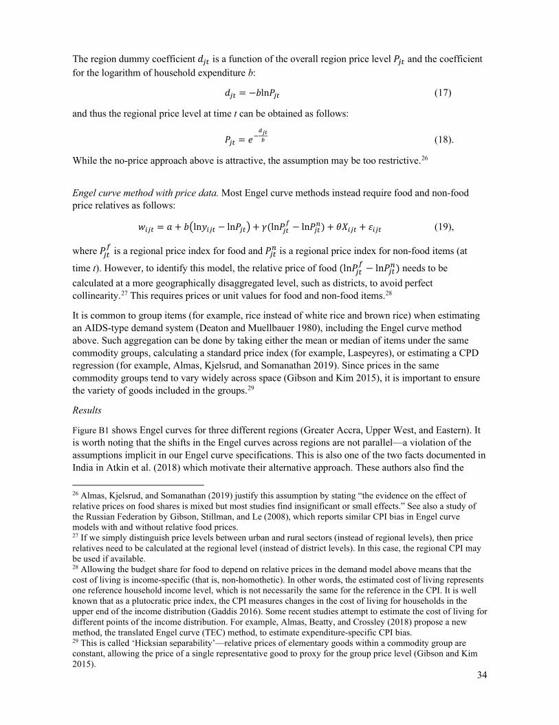
34

The region dummy coefficient 𝑑𝑑𝑗𝑗𝑡𝑡 is a function of the overall region price level 𝑃𝑃𝑗𝑗𝑡𝑡 and the coefficient for the logarithm of household expenditure b:

𝑑𝑑𝑗𝑗𝑡𝑡 = −𝑏𝑏ln𝑃𝑃𝑗𝑗𝑡𝑡 (17)

and thus the regional price level at time t can be obtained as follows:

𝑃𝑃𝑗𝑗𝑡𝑡 = 𝑒𝑒−𝑑𝑑𝑖𝑖𝑗𝑗𝑏𝑏 (18).

While the no-price approach above is attractive, the assumption may be too restrictive.26

Engel curve method with price data. Most Engel curve methods instead require food and non-food price relatives as follows:

𝑤𝑤𝑖𝑖𝑗𝑗𝑡𝑡 = 𝑎𝑎 + 𝑏𝑏�ln𝑦𝑦𝑖𝑖𝑗𝑗𝑡𝑡 − ln𝑃𝑃𝑗𝑗𝑡𝑡�+ 𝛾𝛾(ln𝑃𝑃𝑗𝑗𝑡𝑡𝑓𝑓 − ln𝑃𝑃𝑗𝑗𝑡𝑡𝑛𝑛) + 𝜃𝜃𝐸𝐸𝑖𝑖𝑗𝑗𝑡𝑡 + 𝜀𝜀𝑖𝑖𝑗𝑗𝑡𝑡 (19),

where 𝑃𝑃𝑗𝑗𝑡𝑡𝑓𝑓 is a regional price index for food and 𝑃𝑃𝑗𝑗𝑡𝑡𝑛𝑛 is a regional price index for non-food items (at

time t). However, to identify this model, the relative price of food (ln𝑃𝑃𝑗𝑗𝑡𝑡𝑓𝑓 − ln𝑃𝑃𝑗𝑗𝑡𝑡𝑛𝑛) needs to be

calculated at a more geographically disaggregated level, such as districts, to avoid perfect collinearity.27 This requires prices or unit values for food and non-food items.28

It is common to group items (for example, rice instead of white rice and brown rice) when estimating an AIDS-type demand system (Deaton and Muellbauer 1980), including the Engel curve method above. Such aggregation can be done by taking either the mean or median of items under the same commodity groups, calculating a standard price index (for example, Laspeyres), or estimating a CPD regression (for example, Almas, Kjelsrud, and Somanathan 2019). Since prices in the same commodity groups tend to vary widely across space (Gibson and Kim 2015), it is important to ensure the variety of goods included in the groups.29

Results

Figure B1 shows Engel curves for three different regions (Greater Accra, Upper West, and Eastern). It is worth noting that the shifts in the Engel curves across regions are not parallel—a violation of the assumptions implicit in our Engel curve specifications. This is also one of the two facts documented in India in Atkin et al. (2018) which motivate their alternative approach. These authors also find the

26 Almas, Kjelsrud, and Somanathan (2019) justify this assumption by stating “the evidence on the effect of relative prices on food shares is mixed but most studies find insignificant or small effects.” See also a study of the Russian Federation by Gibson, Stillman, and Le (2008), which reports similar CPI bias in Engel curve models with and without relative food prices. 27 If we simply distinguish price levels between urban and rural sectors (instead of regional levels), then price relatives need to be calculated at the regional level (instead of district levels). In this case, the regional CPI may be used if available. 28 Allowing the budget share for food to depend on relative prices in the demand model above means that the cost of living is income-specific (that is, non-homothetic). In other words, the estimated cost of living represents one reference household income level, which is not necessarily the same for the reference in the CPI. It is well known that as a plutocratic price index, the CPI measures changes in the cost of living for households in the upper end of the income distribution (Gaddis 2016). Some recent studies attempt to estimate the cost of living for different points of the income distribution. For example, Almas, Beatty, and Crossley (2018) propose a new method, the translated Engel curve (TEC) method, to estimate expenditure-specific CPI bias. 29 This is called ‘Hicksian separability’—relative prices of elementary goods within a commodity group are constant, allowing the price of a single representative good to proxy for the group price level (Gibson and Kim 2015).

35

Engel curves in India are not linear. Figure B1 does not show any striking evidence of a nonlinear relationship between the budget share for food and the natural log of household expenditure for most expenditure levels across the three regions. There appears to be some evidence of a nonlinear relationship for low levels of household expenditure; however, this is likely because there are relatively few observations and the local polynomial predictions are noisy at both tails for the three Engel curves.

Figure B1. Engel curves over different regions

Source: Authors’ calculations based on GLSS7.

Figure B2 and Figure B3 summarize the spatial price index estimated by the Engel curve method with and without food/non-food price relatives. The intuition behind the Engel approach is that regions with positive and significant fixed effects are relatively more expensive than Greater Accra. A positive and significant fixed effect estimate suggests that a household devotes a larger share of its household expenditure on food than a comparably similar household in the Greater Accra region. Comparing with our best price estimates in Figure 9, we judge that the Engel-based price measures are not reliable, as, for instance, Greater Accra is unlikely to be a cheap region in Ghana. Thus, in line with Gibson, Le, and Kim (2017), we conclude that the Engel method may not be a reliable tool to measure spatial price levels.

36

Figure B2. Spatial price index based on the Engel curve method (with and without price relatives)

Source: Authors’ calculations based on GLSS7. Note: Spatial price index is normalized so that Greater Accra equals 100.

Figure B3. Spatial price index based on the Engel curve method (all sample and urban subsample)

Source: Authors’ calculations based on GLSS 7. Note: Spatial price index is normalized so that Greater Accra equals 100.

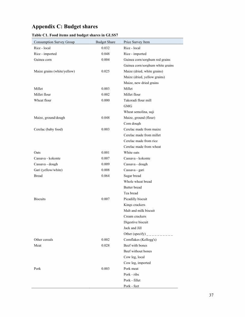
37

Appendix C: Budget shares Table C1. Food items and budget shares in GLSS7

Consumption Survey Group Budget Share Price Survey Item

Rice - local 0.032 Rice - local Rice - imported 0.048 Rice - imported Guinea corn 0.004 Guinea corn/sorghum red grains

Guinea corn/sorghum white grains Maize grains (white/yellow) 0.025 Maize (dried, white grains)

Maize (dried, yellow grains)

Maize, new dried grains Millet 0.003 Millet Millet flour 0.002 Millet flour Wheat flour 0.000 Takoradi flour mill

GMG

Wheat semolina, suji Maize, ground/dough 0.048 Maize, ground (flour)

Corn dough Cerelac (baby food) 0.003 Cerelac made from maize

Cerelac made from millet

Cerelac made from rice

Cerelac made from wheat Oats 0.001 White oats Cassava - kokonte 0.007 Cassava - kokonte Cassava - dough 0.009 Cassava - dough Gari (yellow/white) 0.008 Cassava - gari Bread 0.064 Sugar bread

Whole wheat bread

Butter bread

Tea bread Biscuits 0.007 Picadilly biscuit

Kings crackers

Malt and milk biscuit

Cream crackers

Digestive biscuit

Jack and Jill

Other (specify) _ _ _ _ _ _ _ _ _ _ Other cereals 0.002 Cornflakes (Kellogg's) Meat 0.028 Beef with bones

Beef without bones

Cow leg, local

Cow leg, imported Pork 0.003 Pork meat

Pork - ribs

Pork - fillet

Pork - feet

38

Table C1. Food items and budget shares in GLSS7 (continued) Consumption Survey Group Budget Share Price Survey Item

Mutton 0.001 Mutton chop

Mutton mixed cut Goat 0.005 Sheep - live

Goat - live

Goat meat Chicken 0.005 Live chicken (local)

Live chicken (broiler)

Live chicken (layers) Frozen chicken 0.018 Chicken parts (thighs) - frozen

Chicken parts (wings) Guinea fowl 0.001 Guinea fowl - live Corned beef 0.001 Exeter corned beef

Corned beef (other brands) Sausage (all types) 0.000 Sausage Grasscutter 0.002 Bushmeat (grasscutter) Game bird 0.000 (a) Other meat 0.001 (b) Fresh/frozen fish 0.015 Kpala (starvids) frozen

Fresh river fish

Tilapia - fresh /frozen Shrimps 0.000 Shrimps Snails 0.001 Snails Crab 0.001 Crab Smoked fish 0.058 Smoked river fish Smoked herring/salmon 0.091 Herrings - smoked Fried fish 0.013 (c) Dried fish 0.004 Dried fish - koobi Other fish 0.009 Fish (salted) Sardines/tuna in vegetable oil 0.004 Titus

Princess

Obaapa

Gino

Starkist

Other (specify) _ _ _ _ _ _ _ _ _ _ Mackerel in tomato sauce 0.004 Geisha

African queen

Ena pa

Obaapa

Delay

Other (specify) _ _ _ _ _ _ _ _ _ _ Fresh milk 0.001 Fresh milk

Baby milk (lactogen)

Fan milk

39

Table C1. Food items and budget shares in GLSS7 (continued) Consumption Survey Group Budget Share Price Survey Item

Powdered milk 0.004 Nido milk (sachet)

Peak milk (sachet)

Cowbell (sachet)

Ideal milk (sachet)

Nunu milk (sachet)

Loya milk (sachet)

Miksi milk (sachet)

Vega milk (sachet)

Other (specify) _ _ _ _ _ _ _ _ _ _ Evaporated milk 0.007 Evaporated milk - ideal

Evaporated milk - peak

Evaporated milk - nunu

Evaporated milk - vega

Evaporated milk - carnation Condensed milk 0.000 Condensed milk, tin - peak Other milk products 0.005 Other (specify) _ _ _ _ _ _ _ _ _ _ Chicken eggs 0.009 Chicken eggs (fresh, single) Margarine 0.000 Margarine Coconut oil 0.000 Coconut oil Groundnut oil 0.002 Groundnut oil Palm oil (red oil) 0.008 Palm oil (red oil) Shea butter 0.005 Shea butter Palm kernel oil 0.000 Palm kernel oil Other oils 0.021 Vegetable oil - frytol

Vegetable oil - gino

Vegetable oil - obaapa

Vegetable oil (other, specify) Coconut (fresh/dried) 0.002 Coconut (fresh) Banana 0.005 Banana Oranges 0.003 Oranges Pineapple 0.001 Pineapple Mango 0.001 Mango (local)

Mango (grafted) Watermelon 0.003 Watermelon Avocado pear 0.001 Avocado pear Apples/sweet apple 0.001 Apples (foreign)

Sweet apple Grapes 0.000 Grapes Lime 0.000 Lime Cashew 0.000 (d) Pawpaw 0.001 Pawpaw Other fruits 0.000 (e) Canned fruit 0.000 Canned (processed) fruits

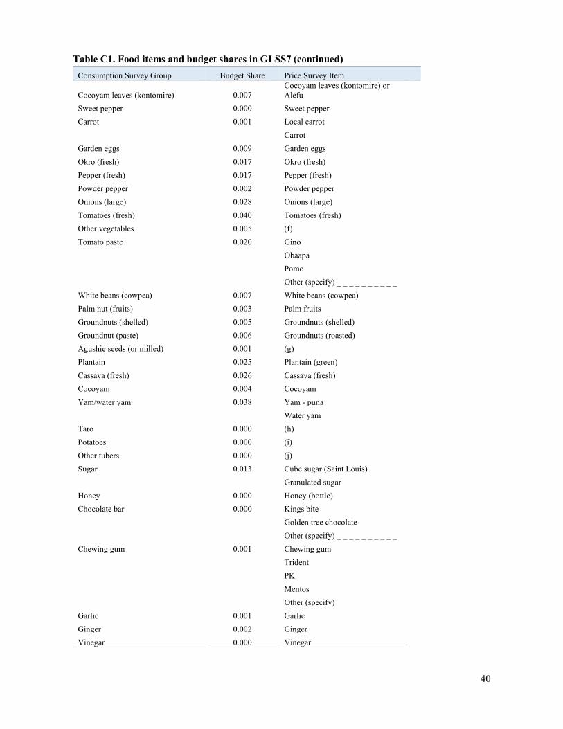
40

Table C1. Food items and budget shares in GLSS7 (continued) Consumption Survey Group Budget Share Price Survey Item

Cocoyam leaves (kontomire) 0.007 Cocoyam leaves (kontomire) or Alefu

Sweet pepper 0.000 Sweet pepper Carrot 0.001 Local carrot

Carrot Garden eggs 0.009 Garden eggs Okro (fresh) 0.017 Okro (fresh) Pepper (fresh) 0.017 Pepper (fresh) Powder pepper 0.002 Powder pepper Onions (large) 0.028 Onions (large) Tomatoes (fresh) 0.040 Tomatoes (fresh) Other vegetables 0.005 (f) Tomato paste 0.020 Gino

Obaapa

Pomo

Other (specify) _ _ _ _ _ _ _ _ _ _ White beans (cowpea) 0.007 White beans (cowpea) Palm nut (fruits) 0.003 Palm fruits Groundnuts (shelled) 0.005 Groundnuts (shelled) Groundnut (paste) 0.006 Groundnuts (roasted) Agushie seeds (or milled) 0.001 (g) Plantain 0.025 Plantain (green) Cassava (fresh) 0.026 Cassava (fresh) Cocoyam 0.004 Cocoyam Yam/water yam 0.038 Yam - puna

Water yam Taro 0.000 (h) Potatoes 0.000 (i) Other tubers 0.000 (j) Sugar 0.013 Cube sugar (Saint Louis)

Granulated sugar Honey 0.000 Honey (bottle) Chocolate bar 0.000 Kings bite

Golden tree chocolate

Other (specify) _ _ _ _ _ _ _ _ _ _ Chewing gum 0.001 Chewing gum

Trident

PK

Mentos

Other (specify) _ _ _ _ _ _ _ _ _ _ Garlic 0.001 Garlic Ginger 0.002 Ginger Vinegar 0.000 Vinegar

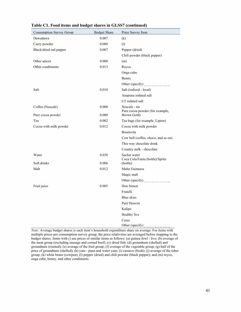
41

Table C1. Food items and budget shares in GLSS7 (continued) Consumption Survey Group Budget Share Price Survey Item

Dawadawa 0.007 (k) Curry powder 0.000 (l) Black/dried red pepper 0.007 Pepper (dried)

Chili powder (black pepper) Other spices 0.000 (m) Other condiments 0.013 Royco

Onga cube

Benny

Other (specify) _ _ _ _ _ _ _ _ _ _ Salt 0.010 Salt (iodized - local)

Anapuna iodated salt

U2 iodated salt Coffee (Nescafe) 0.000 Nescafe - tin

Pure cocoa powder 0.000 Pure cocoa powder (for example, Brown Gold)

Tea 0.002 Tea bags (for example, Lipton) Cocoa with milk powder 0.012 Cocoa with milk powder

Bournvita

Cow bell (coffee, choco, and so on)

This way chocolate drink

Country milk - chocolate Water 0.038 Sachet water

Soft drinks 0.006 Coca Cola/Fanta (bottle)/Sprite (bottle)

Malt 0.012 Malta Guinness

Magic malt

Other (specify) _ _ _ _ _ _ _ _ _ _ Fruit juice 0.005 Don Simon

Frutelli

Blue skies

Pure Heaven

Kalipo

Healthy live

Ceres Other (specify) _ _ _ _ _ _ _ _ _ _

Note: Average budget shares is each item’s household expenditure share on average. For items with multiple prices per consumption survey group, the price relativities are averaged before mapping to the budget shares. Items with () use prices of similar items as follows: (a) guinea fowl - live; (b) average of the meat group (excluding sausage and corned beef); (c) dried fish; (d) groundnuts (shelled) and groundnuts (roasted); (e) average of the fruit group; (f) average of the vegetable group; (g) half of the price of groundnuts (shelled); (h) yam - puna and water yam; (i) cassava (fresh); (j) average of the tuber group; (k) white beans (cowpea); (l) pepper (dried) and chili powder (black pepper); and (m) royco, onga cube, benny, and other condiments.

42

Table C 2. Food items and budget shares in CPI price database

Consumption Survey Group Budget Share CPI Item

Rice - local 0.032 Rice - local Rice - imported 0.048 Rice - imported Guinea corn 0.004 Sorghum white grains

Sorghum red grains Maize grains (white/yellow) 0.025 Maize grains Millet 0.003 Millet Millet flour 0.002 Millet flour Wheat flour 0.000 Wheat flour Maize, ground/dough 0.048 Corn dough

Corn flour (Akpele) Cerelac (baby food) 0.003 Cerelac (baby food)

Cerelac (tin)

Yumvita Oats 0.001 White oats (other cereals)

Quaker Cassava - kokonte 0.007 Cassava - kokonte Cassava dough 0.009 Cassava - processed Gari (yellow/white) 0.008 Yellow gari

Gari Bread 0.064 Bread

Other bread Biscuits 0.007 Biscuit (simple cookie)

Jack and Jill

Ginger biscuits Other cereals 0.002 Indomie or instant noodles

Spaghetti

Other cereal products

Other spaghetti Meat 0.028 Cow meat

Beef without bones

Cow leg, local

Cow leg, imported Pork 0.003 Pork meat

Pork, ribs

Pork, shoulder Mutton 0.001 Mutton Goat 0.005 Goat meat Chicken 0.005 Live chicken

Live chicken, local Frozen chicken 0.018 Frozen chicken Guinea fowl 0.001 Guinea fowl - live Corned beef 0.001 Corned beef

Exeter corned beef

43

Table C2. Food items and budget shares in CPI price database (continued) Consumption Survey Group Budget Share CPI Item

Sausage (all types) 0.000 Sausage Grasscutter 0.002 Bushmeat Game bird 0.000 (a) Other meat 0.001 Dog meat Fresh/frozen fish 0.015 Frozen fish Shrimps 0.000 Shrimps Snails 0.001 Snails Crab 0.001 Crab Smoked fish 0.058 Smoked river fish Smoked herring/salmon 0.091 Fish and seafood Fried fish 0.013 Fish fried Dried fish 0.004 Dried fish - koobi Other fish 0.009 Fish (salted) Sardines/tuna in vegetable oil 0.004 Tuna in vegetable oil

Tuna, canned, starkist

Tuna, canned, geisha

Sardines in vegetable oil Mackerel in tomato sauce 0.004 Mackerel in tomato sauce Fresh milk 0.001 Milk (fresh) Powdered milk 0.004 Powdered milk

Peak (sachet)

Powdered milk (sachet) Evaporated milk 0.007 Evaporated milk

Cowbell (sachet) Condensed milk 0.000 (b) Other milk products 0.005 Fan milk products Chicken eggs 0.009 Chicken eggs (fresh, single) Margarine 0.000 Margarine Coconut oil 0.000 Coconut oil Groundnut oil 0.002 Oils and fats (ND) Palm oil (red oil) 0.008 Palm oil (red oil) Shea butter 0.005 Oils and fats (ND) Palm kernel oil 0.000 Cooking oil Other oils 0.021 Oils and fats (ND) Coconut (fresh/dried) 0.002 Coconut (fresh) Banana 0.005 Banana Oranges 0.003 Oranges Pineapple 0.001 Pineapple Mango 0.001 Mango Watermelon 0.003 Watermelon Avocado pear 0.001 Avocado pear Apples/sweet apple 0.001 Apples (foreign)

Sweet apple

44

Table C2. Food items and budget shares in CPI price database (continued) Consumption Survey Group Budget Share CPI Item

Grapes 0.000 Grapes Lime 0.000 Lemon/lime Cashew 0.000 (c) Pawpaw 0.001 Pawpaw Other fruits 0.000 (d) Canned fruit 0.000 (e) Cocoyam leaves (kontomire) 0.007 Cocoyam leaves (kontomire) Sweet pepper 0.000 Fresh pepper Carrot 0.001 Local carrot

Foreign carrot Garden eggs 0.009 Garden eggs Okro (fresh) 0.017 Okro Pepper (fresh) 0.017 Fresh pepper

Pepper Powder pepper 0.002 Powder pepper Onions (large) 0.028 Onions Tomatoes (fresh) 0.040 Tomatoes Other vegetables 0.005 Fresh vegetables (ND) Tomato paste 0.020 Gino

Lele

Tomato paste White beans (cowpea) 0.007 White beans (cowpea) Palm nut (fruits) 0.003 Palm nut Groundnuts (shelled) 0.005 Groundnuts Groundnut (paste) 0.006 Oils and fats (ND) Agushie seeds (or milled) 0.001 (f) Plantain 0.025 Plantain (green) Cassava (fresh) 0.026 Cassava Cocoyam 0.004 Cocoyam Yam/water yam 0.038 Yam Taro 0.000 (g) Potatoes 0.000 (h) Other tubers 0.000 (i) Sugar 0.013 Sugar/honey Honey 0.000 Sugar/honey Chocolate bar 0.000 Chocolate bar Chewing gum 0.001 Chewing gum Garlic 0.001 Garlic Ginger 0.002 Ginger Vinegar 0.000 Vinegar Dawadawa 0.007 (j) Curry powder 0.000 (k) Black/dried red pepper 0.007 (l)

45

Table C2. Food items and budget shares in CPI price database (continued) Consumption Survey Group Budget Share CPI Item

Other spices 0.000 Cube spices

Benny

Maggi cube (crevette) Other condiments 0.013 (m) Salt 0.010 Salt - iodized Coffee (Nescafe) 0.000 Coffee

Pure cocoa powder 0.000 Pure cocoa powder (for example, Brown Gold)

Tea 0.002 Tea bag Cocoa with milk powder 0.012 Cocoa with milk powder Water 0.038 Mineral water (bottled)

Bottle water

Sachet water Soft drinks 0.006 Soft drink

Fanta (can)

Sprite (bottle)

Coca Cola (can) Malt 0.012 Malt drinks (bottle)

Malt drinks (can) Fruit juice 0.005 Fruit juice

Note: Average budget shares is each item’s household expenditure share on average. For items with multiple prices per consumption survey group, the price relativities are averaged before mapping to the budget shares. Items with () use prices of similar items as follows: (a) guinea fowl - live; (b) evaporated milk; (c) groundnuts; (d) average of the fruit group; (e) half of the average price of the fruit group; (f) half of the price of groundnuts (shelled); (g) yam; (h) cassava; (i) average of the tuber group; (j) white beans (cowpea); (k) powder pepper; (l) powder pepper; and (m) cube spices, benny, and maggi cubes.