How to digitize landuse coverage with Quantum GIS 2.2 – Valmiera

Installing Quantum GIS 2.2 – Valmiera (QGIS) Visit http://qgis.org/downloads/ and download either QGIS-OSGeo4W-2.2.0-1-Setup-x86.exe or

QGIS-OSGeo4W-2.2.0-1-Setup-x86_64.exe, depending on your PC.

After download has finished, run the downloaded installation file. When installation is finished, start

QGIS Desktop 2.2.0. The user interface should look similar to the next image.

Figure 1 QGIS Interface

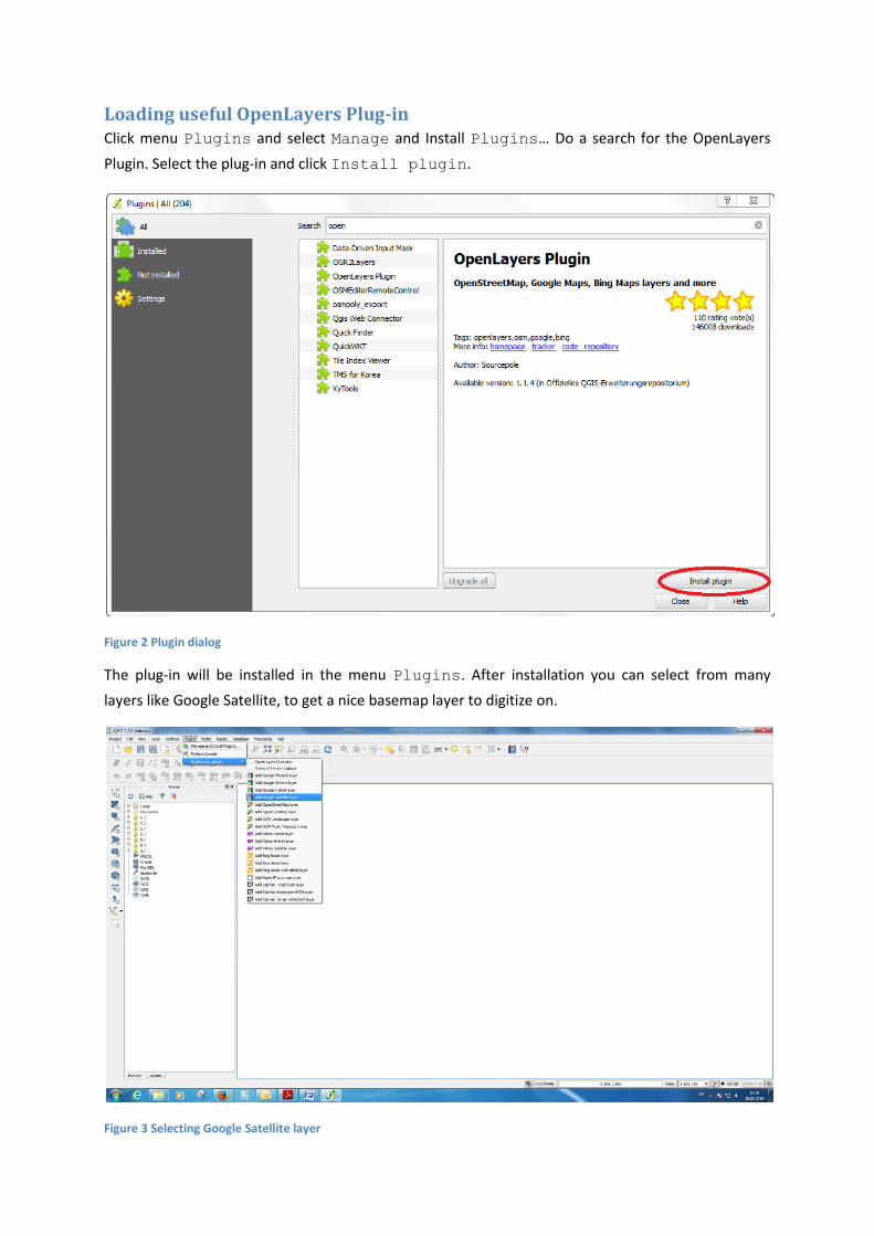
Loading useful OpenLayers Plug-in Click menu Plugins and select Manage and Install Plugins… Do a search for the OpenLayers

Plugin. Select the plug-in and click Install plugin.

Figure 2 Plugin dialog

The plug-in will be installed in the menu Plugins. After installation you can select from many

layers like Google Satellite, to get a nice basemap layer to digitize on.

Figure 3 Selecting Google Satellite layer

You can pan and zoom in this layer just like in GoogleEarth.

Figure 4 Google Satellite layer in map view

Creating landuse coverage Shapefiles in QGIS

Creating a new Shapefile

To create a new shapefile click on New Shapefile Layer on the left side of the QGIS

interface.

Select the type Polygon for a layer that should include areas.

Specify CRS (Coordinate Reference System) WGS84 / UTM zone 37N. This is not a

geographic but a projected coordinate system. Therefore it allows you to perform metric calculations

and it is the appropriate one to digitize spatial features in the project area. You may filter it in the

Specify CRS dialog by its EPSG number 32637.

Figure 5 Specify CRS dialog

In the New Vector Layer dialog remove the attribute id. You probably won’t need it. Add

Attributes that you will need. Name them short and distinctively e.g. “Remark” for an attribute that

will fill to give remarkable information to the feature you will digitize.

Figure 6 New Shapefile Layer dialog

Click OK. Save the file with a short and descriptive name, e.g. “Agriculture” for agricultural areas that

you want to digitize.

Figure 7 Save Layer dialog

Digitizing landuse coverage In menu Project click Project Properties. Check Enable “on the fly” CRS

transformation. Choose the appropriate coordinate reference system WGS 84 / UTM zone

37N.

Figure 8 Project Properties CRS dialog

Add the base layer that you will digitize on. This can be the Google Satellite view from OpenLayers

Plugin or any georeferenced source.

If you have an Image, click Add Raster Layer and choose the one you need from your

storage device.

After you created all the different shapefiles for all the different classes of landuse that you want to

digitize open them in QGIS by clicking Add Vector Layer and selecting them in your storage

device.

You can also drag them from the Browser Panel into the map view. All your layers should now

be displayed at the Layers Panel.

Figure 9 Browser Panel

Figure 10 Layers Panel

Before starting to digitize ensure that you will snap the areas that you will draw to existing ones.

In menu Settings click Snapping Options… Check your area layers.

Set the Mode to vertex (similar to Node).

Set Units to pixels. Choose a Tolerance between 5 and 20 (test it).

Check Avoid Int. to avoid intersecting areas.

Figure 11 Snapping Options

To start digitizing activate the layer you want to edit by clicking on it in the Layers Panel and

press Toggle Editing.

Click on Add Feature to draw a new Feature.

Click along the corners of the area that you want to digitize. You can always undo the last vertexes

(nodes) by pressing the backspace key on your keyboard.

Figure 12 Digitizing polygon feature

Finish the digitizing of one feature by clicking the right mouse button.

Figure 13 Finish digitizing

Fill the Attributes and press OK.

Figure 14 The resulting feature

To get a better view on your base layer when digitizing you can brighten the color of the

Rubberband.

In menu Settings choose Options.

In tab Digitizing click on the Linecolor and lower the value for Sat (saturation).

Figure 15 Brighten Rubberband

Stop editing by clicking on Toggle Editing again.

When digitizing neighboring features snap to the vertexes of the neighboring feature to avoid holes

between the featrures. Vertexes that will be snapped to are highlighted. The snapping ensures that

there won’t be any holes between your created features.

Figure 16 Highlighted snap

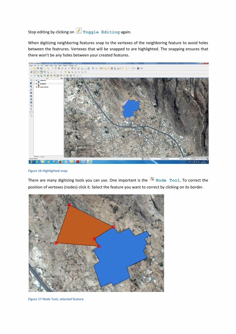
There are many digitizing tools you can use. One important is the Node Tool. To correct the

position of vertexes (nodes) click it. Select the feature you want to correct by clicking on its border.

Figure 17 Node Tool, selected feature

Now you can drag single vertexes to its correct position, you can add nodes by double clicking on the

feature border or you can delete vertexes by selecting them and hitting the delete key on your

keyboard.

Figure 18 Node Tool, selected vertex

You can drag or delete whole features too. To do this, use the appropriate Select Tool. You

can choose the fitting on by clicking on the arrow next to the icon.

Save your editing once in a while to prevent losses in case of software or hardware crashes. Save

your files separately at least once every day you are changing it. Even try to save your results on two

different devices. These backups can be very useful.

The following example illustrates a possible result of digitizing landuse coverage.

Figure 19 Landuse sample

This case represents builded areas classified by density and different forms of vegetation in two

displayed map layers.