How Important is Technological Innovation in Protecting the Environment?

How Important is TechnologicalInnovation in Protecting theEnvironment?

Ian W.H. ParryWilliam A. PizerCarolyn Fischer

Discussion Paper 00-15

March 2000

1616 P Street, NWWashington, DC 20036Telephone 202-328-5000Fax 202 939-3460

© 2000 Resources for the Future. All rights reserved. No portionof this paper may be reproduced without permission of the author.Discussion papers are research materials circulated by their authorsfor purposes of information and discussion. They have notnecessarily undergone formal peer review or editorial treatment.

ii

Abstract

Economists have speculated that the welfare gains from technological innovation that

reduces the future costs of environmental protection could be a lot more important than the

“Pigouvian” welfare gains over time from correcting a pollution externality. If so, then a primary

concern in the design of environmental policies should be the impact on induced innovation, and

a potentially strong case could be made for additional instruments such as research subsidies.

This paper examines the magnitude of the welfare gains from innovation relative to the

discounted Pigouvian welfare gains, using a dynamic social planning model in which research

and development (R&D) augments a knowledge stock that reduces future pollution abatement

costs.

We find that the discounted welfare gains from innovation are typically smaller and

perhaps much smaller than the discounted Pigouvian welfare gains. This is because the long-

run gain to innovation is bounded by the maximum reduction in abatement costs and, since R&D

is costly, it takes time to accumulate enough knowledge to substantially reduce abatement costs.

Only in cases when innovation substantially reduces abatement costs quickly (by roughly 50%

within 10 years) and the Pigouvian amount of abatement is initially modest, can the welfare

gains from innovation exceed the welfare gains from pollution control. These results apply for

both flow and stock pollutants, and for linear and convex environmental damage functions.

Our results suggest that spurring technological innovation should not be emphasized at

the expense of achieving the optimal amount of pollution control. More generally, our results

appear to have implications for a broad range of policy issues. They suggest that the welfare

gains from innovation that reduces the costs of supplying any public good (defense, crime

prevention, infrastructure, etc.) may be fairly small relative to those from providing the optimal

amount of the public good over time.

iii

Table of Contents

1. Introduction 1

2. Basic Results 6

A. Model Assumptions 6

B. Analytic Results 7

Figure 1: Welfare Gains with and without Innovation 8

C. Numerical Simulations 11

Table 1: Calculations of PVI / PVP 13

3. Alternative Assumptions and Sensitivity Analysis 15

A. Discount Rate 15

Table 2: Effect of Alternate Discount Rates ( r ) on PVI / PVP 16

B. Research Costs 17

Figure 2: Cost Reduction Schedules Under Different Alternatives 18

Table 3. PVI/PVP under Alternative Models of Research Costs and Innovation Effects 19

C. Convex Damages 19

Table 4. PVI/PVP for Flow Pollutant with Convex Environmental Damages 21

D. Stock Pollutant 21

E. Innovation and Abatement over Shorter Planning Periods 22

F. Delayed Abatement 23

Table 5: PVI/PVP when Abatement Begins after Ten Years (40% abatement) 24

4. Conclusion 24

References 27

1

How Important is Technological Innovation in Protecting the Environment?

Ian W.H. Parry, William A. Pizer, and Carolyn Fischer1

1. Introduction

When firms are not charged for the harm their activities do to the environment, two types

of resource misallocation can occur. As is well known from the Pigouvian model, at a point in

time firms’ pollution levels will exceed the socially optimal amount. It also is important to

recognize that the state of technology is endogenous over the long run. If firms do not have to

worry about pollution control, they lack incentives to engage in innovative activities that might

lead to cleaner production technologies for future periods. This problem is compounded by the

usual R&D externality: even if firms do invent new abatement technologies, they may be unable

to capture all the spillover benefits to other firms due to the public good nature of knowledge. In

short then, there is both a static and a dynamic source of market failure.

This paper is about the relative importance of the dynamic resource misallocation. More

specifically, we measure the welfare gains from achieving the socially optimal innovation of

cleaner technologies over time, relative to the welfare gains from reaching the optimal amount of

pollution control the “Pigouvian” welfare gains—with technology held constant. This question

crucially bears on the appropriate design of measures to tackle environmental problems in a

variety of different respects.

1 All three authors are at Resources for the Future, 1616 P Street NW, Washington, D.C. 20036. Correspondingauthor: Ian Parry, email: [email protected], phone: (202) 328-5151. We are grateful to Felicia Day, Michael Toman andKaren Fisher-Vanden for helpful comments and to the U.S. Environmental Protection Agency (Grant CX 82625301)for financial support.

PARRY, PIZER, AND FISCHER RESOURCES FOR THE FUTURE

2

First, it is helpful for policymakers to know what is at stake in terms of economic welfare

from policy intervention to address specific environmental problems whether a strong case for

policy intervention can be made or not depends on whether the potential welfare gains are large

or not. Part of this welfare gain consists of the potential to address externality distortions in the

market for environmentally-focussed R&D. Since existing studies usually take the state of

technology as exogenous (e.g., the survey in Cropper and Oates (1992)), they ignore this

opportunity to improve welfare and understate the potential efficiency gains from environmental

policies.

Second, the size of the welfare gain from induced innovation can bear directly on the

appropriate choice of environmental policy instrument. As demonstrated in earlier studies,

different environmental policy instruments are likely to induce different amounts of R&D (e.g.,

Milliman and Prince (1989), Jung et al. (1996), Parry (1998), Fischer et al. (1999)). Therefore,

the welfare effects of policies that are equivalent (under certain conditions) in a static, partial

equilibrium framework such as emissions taxes, grandfathered permits, and auctioned

permits can differ when technological innovation is endogenous. However, whether these

differences are likely to matter much in practice depends on how significant the welfare gains

from innovation are, relative to the Pigouvian welfare gains.2 A related point is that technological

innovation may affect the optimal stringency of environmental regulations.3 Again though,

whether the optimal deviations from the Pigouvian rule matter much in practice depends on the

relative economic importance of induced innovation effects.

Finally, if in the presence of environmental policies the patent system is not especially

effective at enabling innovators to capture the full social benefits from new abatement

2 In a competitive setting, Fischer et al. (1999) find that there is no clear-cut ranking between emissions taxes, freetradable emissions permits, and auctioned permits. Under certain conditions concerning the potential for innovation,the degree to which non-innovating firms can imitate new technologies, and the degree of convexity of the pollutiondamage function, any one of these three instruments may induce a larger welfare gain than the other two. Forexample, they find that emissions taxes tend to induce larger welfare gains when marginal environmental damagesare relatively constant and the potential for imitating new technologies is limited.3 For example, Parry (1995) shows that the second-best optimal pollution tax may exceed marginal environmentalbenefits when, despite patents, innovators are unable to appropriate the full benefits to other firms from newtechnologies. On the other hand, competition for a given amount of innovation rent can be socially excessive, in thesame way that competition can lead to the overuse of natural resources. This “common pool” effect tends to dampenthe optimal pollution tax.


3

technologies, additional measures to stimulate R&D may be justified. Examples include research

subsidies, tax credits, or technology prizes. The case for introducing these supplementary

measures, and the optimal amount of rewards involved, depends on the potential welfare gains

from additional innovation.

In fact, in the long run technological innovation seems to be at the heart of resolving a

number of problems with seemingly irreconcilable conflicts between economic activity and the

environment. For example, governments have so far been unwilling to accept the economic costs

that would be necessary to fulfill promises made eight years ago at the 1992 Earth Summit to

stabilize let alone reduce substantially emissions of heat-trapping gases.4 The development of

carbon-saving technologies over time (e.g., improved techniques for using natural gas in power

generation, hybrid cars, etc.) offers the hope of meeting emissions controls in the future with less

burden imposed on industry and consumers. Similarly, the development of improved auto

exhaust filters for nitrogen oxide emissions could substantially reduce smog in urban areas such

as Los Angeles, thereby obviating the need for draconian restrictions on vehicle manufacture in

order to meet federal air quality standards. Thus, economists have suggested that the welfare

gains from technological innovation might be “large” and that the impact of environmental

policies on innovation should be the most important consideration in policy design.5

Very little is known from previous literature about the potential welfare gains arising

from the impact of environmental policies on technological innovation.6 In this paper we attempt

to provide a general treatment of this issue, using a dynamic social planning model in which the

control variables in each period are the amount of pollution abatement and the amount of R&D

4 At the 1997 Kyoto conference, the developed countries again pledged to reduce emissions. But the timetable forimplementing emission targets was pushed back to 2008-2012 almost 20 years after governments first pledged tocontrol emissions. Moreover, there is widespread skepticism that the agreement will be adopted in anything like itscurrent form (e.g, Portney, 1999).5 For example, Kneese and Schultz (1978): “ Over the long haul, perhaps the single most important criterion onwhich to judge environmental policies is the extent to which they spur new technology towards the efficientconservation of environmental quality.” Orr (1976): “Technological adaptation rather than resource allocation [is]the key to an effective solution of [environmental problems].”6 There are a couple of studies that use numerical simulation models to estimate how endogenous technologicalchange affects the optimal level of carbon taxes (e.g., Nordhaus (1998) and Goulder and Matthai (2000)). We relateour results to these studies below. Parry (1998) and Fischer et al. (1999) estimate what fraction of the first-best


4

investment. R&D enhances a knowledge stock, which reduces the future costs of abatement. We

define the discounted Pigouvian welfare gain (PVP) as the present value of welfare gains from

the socially optimal amount of pollution abatement in each period (relative to no abatement)

when the state of technology is exogenous. We then solve for the discounted welfare gains from

reaching the first-best level of abatement and R&D in each period (relative to no abatement and

no R&D), when the state of technology is endogenous. The difference between these welfare two

measures is the discounted welfare gain from innovation (PVI).

The basic finding is that the conditions for PVI to exceed PVP are actually quite stringent,

and in fact PVI could easily be small relative to PVP. For example, even under conservative

assumptions, we find that when the initial Pigouvian abatement level is 40% then innovation

(and diffusion) must reduce abatement costs by 50% within 10 years, and by a much greater

amount over the longer term, for PVI to be as large as PVP. It is practically inconceivable that

this condition could be met, for example, in the context of carbon abatement, given our current

dependency on fossil fuels. The condition becomes even more stringent, if not impossible, to

satisfy when the Pigouvian amount of abatement is initially in excess of 60%. Our results apply

for flow and stock pollutants, for linear and convex environmental damage functions, and when

the welfare gains from innovation and abatement are compared over shorter periods within of

time.

The limited welfare gains from innovation initially surprised us, but the result makes

intuitive sense. We can bound the maximum possible benefit from innovation in a particular

period when abatement costs have been completely eliminated by a simple trapezoid under

the marginal abatement cost and marginal environmental benefit curves (see below). It is easy to

show that the ratio of this trapezoid to the Pigouvian welfare gain triangle is 9, 3, and 1 when the

initial Pigouvian level of abatement is 20%, 50%, and 100%, respectively. This reflects the fact

that when a pollution externality is severe enough to warrant significant reductions based on

current control costs, the Pigouvian social benefit from optimal pollution reduction will be large

relative to the potential cost savings from innovation. However, this ratio greatly overstates

________________________

welfare gains from innovation are obtained under alternative environmental policies, but they do not estimate thesize of these gains relative to the Pigouvian welfare gains.


5

PVI/PVP for two reasons. First, on the optimal path it will take decades (if not longer) to

completely eliminate abatement costs; hence, for a whole range of future periods the benefit

from innovation relative to the Pigouvian welfare gain is much smaller than these ratios suggest.

Second, we need to subtract the costs of R&D from the benefits in order to obtain the net welfare

gain.

The bottom line is that, at least in terms of social welfare, promoting technological

innovation appears to be less important than just controlling pollution, contrary to what some

economists previously have speculated. Accordingly, it seems that the primary objective of

environmental policy should be the traditional one of achieving the optimal amount of pollution

control over time and promoting innovation should be a secondary concern. This conclusion is

preliminary however, because, as discussed later, there are some notable caveats to our analysis.

In particular, our analysis does not capture possible spillover benefits to other industries from

induced innovation. We do not take into account sources of pre-existing distortion in the

economy that may importantly influence the overall welfare effects of environmental policies.

These caveats aside, our results appear to have implications for a broad range of other

(non-pollution-related) policy issues. The results suggest that the welfare gains from improving

technologies for fish farming are likely to be smaller than the welfare gains from limiting access

to natural fish stocks. Similarly, the welfare gains from developing safer consumer products are

likely to be smaller than those from enforcing safety standards based on existing technologies.

Again, the reason is that innovation is costly and it takes time for innovation to secure a

substantial reduction in the costs of fish farming or product safety. More generally, the results

suggest that the welfare gains from innovation that reduce the cost of supplying almost any

public good (defense, crime prevention, infrastructure, etc.) are likely to be smaller than those

from providing the optimal amount of the public good over time.

The rest of the paper is organized as follows. Section 2 lays out our analytical framework

and develops our main qualitative and quantitative results. Section 3 relaxes some of the

simplifying assumptions in Section 2 and conducts further sensitivity analyses. Section 4

concludes and discusses limitations to the analysis.


6

2. Basic Results

A. Model Assumptions

Consider an industry where a by-product of production is waste emissions that are

detrimental to environmental quality. These emissions may represent air or water pollutants,

hazardous or other forms of solid waste, radioactive materials, and so on. In the absence of any

abatement measures, economy-wide emissions per period (“baseline” emissions) would be an

exogenous amount E . The cost of reducing emissions by an amount At below E at time t, or

emissions abatement, is C(At, Kt). Kt denotes the stock of knowledge about possibilities for

reducing emissions. A higher value of Kt may represent, for example, improved techniques for

replacing coal with natural gas in electricity generation, or a more efficient end-of-pipe

technology for treating pollution. We assume that marginal abatement costs are upward sloping

and pass through the origin for a given knowledge stock, and that more knowledge rotates the

marginal abatement cost curve downwards about the origin but at a diminishing rate.7 In short

CAA > 0, CA(0, Kt) = 0, CAK < 0, CAKK > 0.

Knowledge accumulates as follows:

(1) ttt IKK +=+1

where K0 is given and It is investment in environmentally orientated R&D activities.8 The

cost of R&D is f(It) where f(.) is weakly convex. To keep the model parsimonious, and the results

conservative, diffusion is subsumed in f(.).9

Emissions accumulate in the environment over time as follows:

(2) 1)1( −−+−= ttt SAES δ

7 The assumption that the marginal cost schedule passes through the origin is an important assumption and isconsistent with the shadow value of pollution equaling zero. This would not be the case in the presence of pre-exisiting distortions, such as energy subsidies.8 There is no knowledge depreciation; that is, knowledge cannot be disinvented.9 Implicitly then, when we say that innovation has reduced abatement costs by x%, we mean the technologies havebeen invented and fully diffused. Explicitly incorporating a diffusion lag would have essentially the same effect asincreasing the adjustment cost associated with R&D (i.e., assuming a larger f′′ ), and we consider a wide range ofscenarios for adjustment costs in our simulations.


7

where St denotes the stock of pollution in the environment at time t and the inherited

stock S0 is given. δ is the decay rate of the stock: δ = 1 for a flow pollutant which decomposes

before the start of the next period (this is roughly applicable to sulfur dioxide, nitrous oxides, and

particulates). For stock pollutants that accumulate in the environment over time, we have

10 <≤ δ (e.g., nuclear waste and carbon dioxide).

Environmental damages at a point in time are given by φ(St) where φ′ > 0, φ′′ ≥ 0.

Finally, a social discount rate of r is applied to future benefits and costs, and the planning period

extends over an infinite horizon.

B. Analytic Results

For the purposes of this section, we make some simplifying assumptions to establish our

main results in a transparent manner most of these assumptions are relaxed later. We focus on a

flow pollutant (δ = 1) with constant marginal environmental damages from emissions/constant

marginal benefits from abatement equal to φ >0. R&D costs are assumed to be linear ( 0=′′f ).

In addition, we use a quadratic abatement cost function:

(3) 2/))(1(),( 20 cAKKzKAC −−=

where z(.) is the proportionate reduction in abatement costs brought about by innovation

(0 ≤ z ≤ 1, z′ > 0, z′′ < 0 and z(0) =0). For accounting convenience, we also assume that

abatement occurs from t = 1…∞, while innovation can occur in period zero.

For the moment, suppose the state of technology is exogenous, as in the traditional

Pigouvian model, and knowledge is fixed at K0 for the planning horizon. The optimal Pigouvian

abatement level is the point where marginal abatement costs equal marginal environmental

benefits. Using (3), this gives cAP /φ= for t = 1…∞ and the resulting Pigouvian welfare gain

per period, WP, is triangle 0pq in Figure 1.


8

Figure 1: Welfare Gains with and without Innovation

abatement

mar

gina

l cos

ts/b

enef

its

ΜB = φ

MC = CA(A,K0) = cA

AP

MC = CA(A,K*) = c(1 – z*)A

A*0

pq

r

s

E

t

u

We define PVP as the present discounted value (as of t = 0) of the Pigouvian welfare

gains summed from t = 1 to ∞:

(4) ( ) ( ) r

W

r

W

r

W

r

WPV

PPPPP =+

++

++

+= !

32 111

When we allow for innovation, the social planning problem becomes:

(5)( ) ( ) ( )

( )∑∞

= +++−

+1

0, 1

,)(Min

tt

tttt

IA r

IfKACAEIf

tt

φ

subject to ttt IKK +=+1

That is, the planner chooses abatement and innovation in order to minimize the

discounted sum of environmental damages, abatement costs, and innovation costs. Using (3) the

first order conditions yield:

(6)

−−

= EcKKz

At

t ,))(1(

Min0

*

* φ

(7) ( )

r

IfKACIf tttK

t +′+−

=′ +++

1

),()(

*1

*1

*1*


9

From (6), Pt AA >* : optimal abatement is now greater than in the Pigouvian case because

innovation shifts down the marginal abatement cost curve. Note that if φ<− Ecz )1( * , we have a

corner solution with EA =* and emissions abatement equal to 100% (in Figure 1, EA <* ).

Equation (7) is an Euler equation specifying that the marginal cost of R&D in period t

equals the (discounted) reduction in abatement costs in period t+1 from an increase in the

knowledge stock, plus the marginal cost of R&D in period t+1. With our assumption of linear

R&D costs, frKAC ttK ′=− ),( ** . Along with (6) we have two static equations providing implicit

solutions for K* and A*. Thus, abatement and the knowledge stock are constant over t = 1…∞

and R&D must occur only in period 0 (this is unrealistic, but simplifies our discussion and makes

our initial results conservative see below).

In any given period, the benefit from having a knowledge stock equal to K* rather than K0

is denoted WK, and is indicated by triangle 0qr in Figure 1. This consists of the reduction in

abatement costs at the Pigouvian amount of abatement (triangle 0qs) plus the gain from

increasing abatement from PA to *A (triangle qrs). Using some simple geometry:

(8)

−>∆−−

−=−=

EzcifWz

z

AzcifWz

z

WP

P

K

)1(1

)1(1

**

*

***

*

φ

φ

where ( ) ( ) 0)1(2)1( *2* >−−−=∆ czEczφ . ∆ is positive only in the corner solution

where abatement equals 100%, and abatement cannot increase up to the point where marginal

abatement costs equal φ.

We define the welfare gain to innovation, PVI, as the discounted sum of benefits from

additional knowledge (K* − K0) in each period, less the cost of R&D which occurs in period zero.

Thus:

(9) )()(...)1()1(1

*0

*032

Ifr

WIf

r

W

r

W

r

WPV

KKKKI −=−+

++

++

+=

Using (4) the welfare gain from innovation relative to the discounted Pigouvian welfare

gain is:


10

(10)P

K

P

K

P

I

W

IrfW

rW

IfrW

PV

PV )()( *0

*0 −

=−

=

Thus the (discounted) welfare gain from innovation is greater (less) than the (discounted)

welfare gain from correcting the pollution externality, when PVI/PVP is greater (less) than unity.

We now establish two analytic results that bound the magnitude of PVI/PVP:

(i) If 1/ ≤EAP is the optimal (i.e. Pigouvian) proportionate emissions reduction with no innovation,

then 1)/(2 1 −−EAP is the absolute maximum value of PVI/PVP.

Proof: Suppose that innovation completely and costlessly eliminates abatement costs in

the initial period. In this case PVI/PVP is simply WK/WP, or area 0qtu in Figure 1 divided by

triangle 0pq. Since area 0pq equals 2/PAφ and area 0qtu equals )(2/ PP AEA −+φφ , then

PVI/PVP equals 1)/(2 1 −−EAP .

(ii) If R&D reduces abatement costs by a factor z, then PVI/PVP cannot exceed z/(1−z).

Proof: Using (8) and (10),

z

z

W

IrfWz

z

W

IrfW

PV

PVP

P

P

K

P

I

−≤

−∆−−=

−=

1

)(1)(

*0*

0

since ∆ and f(.) ≥ 0 •

Result (i) puts an upper bound on PVI/PVP for the case when knowledge accumulation

completely eliminates abatement costs at zero cost. According to this formula, when the initial

Pigouvian abatement level is 10%, 40%, 60%, or 100%, then the maximum value of PVI/PVP is

19, 4, 2.3, or 1 respectively. Straight away, we see that only in cases when the Pigouvian

abatement level is fairly modest is there potential for the welfare gains from innovation to be

“large” relative to the Pigouvian welfare gains. Intuitively, if a pollution problem is severe

enough to warrant a high level of abatement without R&D, then the additional gain to innovation


11

will be relatively small.10 Conversely, if abatement is initially too costly to justify major

emission reductions, the gain to innovation could be more substantial.

Result (ii) puts an upper bound on PVI/PVP for the case when innovation does not

completely eliminate abatement costs. Here we see that PVI/PVP cannot exceed unity if

innovation reduces abatement costs by 50% or less. In short then, these simple results

demonstrate that there are two necessary conditions for the welfare gains from innovation to be

large relative to the Pigouvian welfare gains: innovation must have the potential to substantially

reduce abatement costs and the initial Pigouvian abatement level must be fairly modest.11

It is worth noting that these bounds are easier to establish—and more conservative—

when one ignores benefits and only considers cost-effectiveness. Cost-effectiveness focuses on

the cost of alternative policies designed to achieve the same emission or abatement target, taking

that target as given (Newell and Stavins, 2000; Hahn and Stavins, 1992). This approach is

appealing because it both avoids contentious discussion of benefits and disentangles the

abatement goal (often a political issue) from the choice of policy design (frequently an

administrative concern). Yet, the underlying assumption behind the target choice, if it reveals

social preferences, must be that marginal benefits equal or exceed marginal costs at the chosen

target. With linear marginal abatement costs and flat marginal benefits, this indicates that the

upper bound (with costless and complete elimination of abatement costs) for PVI/PVP is, at most,

one when the target remains fixed.

C. Numerical Simulations

While the previous results establish unambiguous bounds on the gain to innovation, they

overstate the actual value of PVI/PVP for two reasons. First, we need to subtract the direct costs

of R&D in order to obtain the net welfare gain from innovation. Second, in general it will be

10 Thus, without doing any estimation we can say that PVI is unlikely to exceed PVP for pollutants for which thePigouvian pollution reduction is close to or equal to 100%. This appears to be the case for lead emissions fromgasoline, which cause adverse human health effects, and CFC emissions, which deplete the ozone layer (seeNichols, 1997, and Hammitt, 1997, respectively).11 Note that the maximum value of PVI/PVP is given by the smaller of the values from the two formulas. Thus, whenz = .8 and AP = .8, the maximum value of PVI/PVP is 1.5, while if AP = .2 and z = .4, the maximum value is .67.


12

optimal to smooth out knowledge accumulation over time rather than doing it all in period zero

(i.e. f′′ is typically positive). Hence, for a whole range of future periods, the benefit from

knowledge accumulation will be smaller than the benefits in the steady state when knowledge

accumulation is complete.

Therefore, we now generalize the model to allow for convex R&D costs. Smoothing out

R&D over time involves striking a balance between the gains of immediate increases in the

knowledge stock and the cost savings from gradual adjustment. This is captured by the Euler

equation (7) which matches the marginal R&D cost difference in adjacent periods to the one-

period return to R&D. The solution to the problem with adjustment costs cannot be completed

analytically and therefore we turn to numerical simulations.

For this section we now specify a convex research cost function:

(11) 221)( ttt IfIfIf +=

with f1, f2 > 0. The parameter f1 determines knowledge capital in the steady state: the

lower the value of f1 the more likely that it will be optimal to (eventually) accumulate enough

knowledge to reduce abatement costs by 100%. f2 determines the speed of adjustment to the

steady state: the smaller f2 is, the shorter the period of transition to the steady state will be. The

justification for f2 > 0 is that it is increasingly costly to increase the knowledge stock all at

once at any point in time, there is a limited pool of expert engineers/scientists as well as

specialized capital equipment such as research labs. 12

We then specify the proportionate shift in the abatement cost function due to knowledge:

(12) 22 )1(12)( KKKKz −−=−=

which satisfies z(0) = 0, z′ > 0 for K < 1, and max(z) = z(1) = 1. Note that the choice of K0

is arbitrary since only the distance K – K0 matters. We therefore choose K0 = 0 and, from (12), Kt

= 1 achieves a 100% reduction in abatement costs.

To start with, we choose f1 = 0 which guarantees in the steady state that the knowledge

stock will completely eliminate abatement costs since marginal R&D is now costless. Since our

12 Similarly, doubling the number of people (with comparable skills) working on this paper will reduce theproduction time by less than 50%.


13

aim is to identify an upper bound for PVI/PVP in different situations, this assumption also makes

our results conservative relative to f1 > 0 (from (10), higher values of f′ imply lower relative

welfare gains to innovation). Emissions and environmental damages are normalized to imply

1=E and φ = 1. We assume the discount rate r equals 5% (alternative values are discussed

later).

The remaining parameters, c and f2, are varied. We choose c to imply that the Pigouvian

amount of abatement (AP = φ / c) either is 10%, 40%, or 60%. Finally, we select different values

of f2 in order to imply a wide range of scenarios for the time it takes for knowledge accumulation

to produce a 50% reduction in abatement costs (i.e., half the eventual reduction in abatement

costs). The results of our benchmark simulations are summarized in Table 1.

Table 1: Calculations of PVI / PVP

Time lag until abatement costs halvePigouvian

abatement level 0 10 years 20 years 40 years

10% 19.00 2.98 0.88 0.16

40% 4.00 1.07 0.46 0.16

60% 2.33 0.79 0.41 0.17

In the first column, we set f2 = 0; consequently, innovation completely and immediately

eliminates abatement costs at zero cost. These entries confirm our earlier calculations about the

absolute maximum value of PVI/PVP.

The next three columns show the effect of incorporating positive and increasingly higher

adjustment costs. Suppose the initial Pigouvian abatement level is 40%. In this case, the welfare

gain from innovation, defined in Equation (5), is 107%, 46%, and 16% of the Pigouvian welfare

gains, defined in Equation (6), when innovation reduces abatement costs by 50% over 10, 20,

and 40 years, respectively, along the optimal dynamic path. As predicted earlier, these ratios are

higher (lower) if the initial Pigouvian abatement level is smaller (larger). But regardless of the


14

initial Pigouvian abatement levels in this table, PVI is less than PVP if it takes 20 years or more

for innovation to secure a 50% reduction in abatement costs. Indeed, if the Pigouvian abatement

level is initially 60% or more, then PVI is still less than PVP if a 50% reduction in abatement

costs is secured in only 10 years.

These simulations demonstrate our basic point: the conditions for PVI to be large relative

to PVP seem to be rather stringent. Innovation must rapidly reduce abatement costs by more than

50% and the initial Pigouvian level of abatement must be modest. If high levels of abatement are

initially justified regardless of cost, if cost-savings from innovation are small, or if these cost-

savings occur with a substantial time lag, then PVI is unlikely to be as large as PVP.13

How long, then, might it take for technological innovation to substantially reduce

abatement costs? The sulfur-trading program which ultimately will reduce emissions by about

50% is often heralded as a major success because control costs are now much lower than

initially projected. According to Burtraw (1996), abatement costs roughly halved over 10 years.

This suggests that PVI could be roughly the same size as PVP in this case. However, not all of

this cost reduction was due to induced innovation; a substantial portion appears to have resulted

from the reduction in costs of transporting low sulfur coal brought about by deregulation of the

trucking industry—a change unrelated to the sulfur reduction program. In the context of climate

change, the United States is currently pledged to reduce carbon emissions to 93% of 1990 levels

by 2008-2012 under the Kyoto Protocol. This will imply an emissions reduction of about 30%

below baseline levels (EIA, 1999, p. 89). In this case, the prospects for innovation to

substantially cut abatement costs are less promising since there currently are no end-of-pipe

treatment technologies nor cost-effective, carbon-free alternatives to fossil fuels on the horizon.

It seems unlikely to us that U.S. dependency on coal and petroleum could be cut by 50% in 10-

15 years through innovation.14

13 Another way to interpret these results is that incorporating the cost of R&D can dramatically reduce the potentialwelfare gains from innovation. For example, when the Pigouvian abatement level is 10% we see that without anycosts to R&D the welfare gain from innovation is 19 times the Pigouvian welfare gain. But with R&D costs, thewelfare gain from innovation falls to 80% of the Pigouvian welfare gains when it takes 20 years for knowledgeaccumulation to reduce abatement costs by 50%.14 Consistent with these observations, Nordhaus (1998) and Goulder and Mathai (2000) find that allowing forendogenous technological innovation does not substantially change the overall welfare gains from a carbon tax.


15

Based on our assessment of the likely rate of induced innovation, the discounted welfare

gains from innovation are probably going to be smaller and perhaps much smaller than the

discounted welfare gains from correcting the pollution externality.15 However, this result is based

on a model that is simplified in a number of respects. We now consider how robust this finding is

to a variety of generalizations and sensitivity analyses.

3. Alternative Assumptions and Sensitivity Analysis

In this section we discuss the implications of alternative discount rates, research cost

functions, nonlinear environmental damages, stock pollutants, planning horizons, and

abatement/innovation timing.

A. Discount Rate

In the previous section we assumed a discount rate of 5%. However, there is considerable

dispute over the appropriate discount rate to use: the Office of Management and Budget

recommends a rate of 7%, while some economists argue for a much lower rate in the context of

long-range environmental problems.16

Qualitatively, the main point is that a higher (lower) discount rate reduces (increases) the

relative welfare gains from innovation. This is because the benefits from innovation occur across

a range of future periods while the costs are up-front. Therefore, higher discount rates lower the

annualized net benefits of innovation. In contrast (at least for the flow pollutant) benefits and

costs from pollution abatement occur simultaneously and the discount rate has no effect on

15 Of course this result does not necessarily imply that innovation is unimportant in absolute terms, only that it isprobably less important than directly addressing uncorrected pollution externalities. Furthermore, there is nothingincorrect with the argument that new technologies offer the hope of ameliorating unpalatable tradeoffs in the shortrun between environmental concerns and economic activity. However, the above results remind us that whencomparing the welfare gains from pollution abatement in the short run versus the welfare gains from knowledgeaccumulation over the long haul, discounting can greatly reduce the relative size of the latter effect.16 See Portney and Weyant (1999) for a recent discussion of different viewpoints on discount rates.


16

annualized net benefits.17 The net effect of varying the discount rate between 2% and 8% on

PVI/PVP is shown in Table 2.18

The first three columns confirm the analytic results in (10) in the case with no R&D

costs. In this case the benefits from innovation and the Pigouvian welfare gain are the same in

every period so the discount rate has no effect on their ratio. Hence the upper bound values for

PVI/PVP are unaffected by changing r.

Table 2: Effect of Alternate Discount Rates ( r ) on PVI / PVP

Time lag until abatement costs halve

0 10 years 20 years 40 yearsPigouvian

abatement level

=2% =5% =8% =2% =5% =8% =2% =5% =8% =2% =5% =8%

10% 9.0 9.0 9.0 .00 .98 .36 .05 .88 .28 .39 .16 .08

40% .00 .00 .00 .13 .07 .63 .32 .46 .22 .63 .16 .07

60% .33 .33 .33 .37 .79 .52 .92 .41 .23 .52 .17 .09

In the remaining columns, varying the discount rate significantly affects the size of

PVI/PVP. For a particular time lag until abatement costs are halved, we see from Table 2 that

using a discount rate of 8% rather than 5% roughly halves the value of PVI/PVP, while using 2%

rather than 5% can easily increase PVI/PVP by a factor of two or three. Thus, for example, when

the Pigouvian abatement level is 40% and innovation reduces abatement costs by 50% in 10

years, varying the discount rate between 2% and 8% produces values of PVI/PVP between 2.13

and 0.63.

17 This result is easy to see for the simplified case of no adjustment costs in the last term in (10).18 We also adjust the research cost parameter f2 to keep constant the time lag until abatement costs halve.


17

The possibility of a low discount rate raises the potential importance of innovation and

increases the range of outcomes under which the welfare gains from innovation dominate the

Pigouvian welfare gains. In particular, the gain to innovation with an arbitrarily low discount rate

is limited only by the Pigouvian abatement level and the long-run cost reduction, as shown in

Section 2B. Our conclusions, however, continue to focus on the assumption that 5% represents

the most plausible case (e.g., discussions in Nordhaus, 1994).

B. Research Costs

We now consider the assumptions concerning research costs f(.) and the impact of

increased innovation z(.). The specification of these functions determines the relative gain to

innovation within the theoretical bounds established in the earlier section. That is, f(.) and z(.)

determine the amount of innovation, the implied cost reductions, and the timing of those

reductions—but this must be between zero and the maximal gain when abatement costs are

immediately and costlessly reduced to zero. Our original choice of 221)( ttt IfIfIf += with f1 =

0 and 2)1(1)( KKz −−= creates a smooth R&D path that asymptotically drives abatement costs

to zero (since marginal R&D is costless).

Holding this path of cost reductions fixed, higher research costs unambiguously lower the

relative welfare gain from innovation since the Pigouvian welfare gain is unaffected and the gain

to innovation net of research costs is lowered. Since it is easy to conjecture that R&D costs could

be large and might even exceed the benefits to innovation, we instead focus on the consequences

of lowering the cost of innovation. This allows us to bound the maximal gain to innovation

conditional on a particular path of cost reductions.

Let us specify a particular path for cost reductions—a reduced form, in some sense, for

f(.) and z(.)—and then compute the relative gain to innovation ignoring any R&D costs. This

separates the issue of R&D costs from the issue of innovation lag, allowing us to disentangle

their relative importance. For simplicity, we consider a linear path of abatement cost reductions,

removing the ambiguity of how research costs are determined by f(.) and how a non-linear path

of cost reductions might be determined by f(.) and z(.). For reference, Figure 2 shows the

endogenous, optimal path of cost reductions, z(Kt), associated with our earlier “20 year lag until

abatement costs halve” specification for both the 10% and 40% Pigouvian abatement levels,


18

alongside this linear alternative. Note that our original quadratic specifications for f(.) and z(.)

generates roughly linear cost reductions up to 50%, and moves asymptotically toward 100% at

different rates depending on the initial abatement level. Intuitively, this occurs because once the

abatement level itself reaches 100%, the marginal gain to innovation begins to diminish since,

looking back to Figure 1, the additional gain qrs no longer exists.

Figure 2: Cost Reduction Schedules Under Different Alternatives

0 20 40 60 80 1000

0.2

0.4

0.6

0.8

1

10% initial abatement40% initial abatementlinear cost reductions

year

cost

red

uctio

n

Implementing the linear reduction schedule as exogenous and costless innovation over

time, we re-compute the relative gain to this innovation in Table 3. With R&D costs removed,

this reflects the pure effect of a time lag in innovation, assuming linear cost reductions. The main

story from Table 3 is that at ten years, half the maximal gain to innovation is lost entirely due to

delay. When innovation requires forty years to halve abatement costs—an annual decline in

abatement costs of 1.25% per year—the gain to innovation is equal to or smaller than the

Pigouvian gain in all cases.


19

Table 3. PVI/PVP under Alternative Models of Research Costs and Innovation Effects

Time lag until abatement costs halvePigouvian

abatement level (%)Innovation Model

0 10 years 20 years 40 years

10original

quadratic z & f19.00 2.98 0.88 0.16

costless linearreductions

19.00 8.61 3.95 1.01

40original

quadratic z & f4.00 1.07 0.46 0.16


4.00 2.25 1.31 0.55

60original

quadratic z & f2.33 0.79 0.41 0.17


2.33 1.42 0.90 0.44

The relative gain to innovation with costless linear reductions in abatement costs is

remarkably similar to the effect of using a 2% discount rate in Table 2. Like the discount rate,

alternate assumptions about research costs raise the gain to innovation, limited first by the

theoretical bounds established in Section 2B, and now further limited by the time lag until costs

are halved. However, it seems reasonable to believe that any time lag in innovation arises

because of an endogenous decision about R&D. For that reason we continue to focus on our

quadratic model of f(.) and z(.). With marginal R&D costs starting at zero, we believe this

already represents a conservative model of R&D costs.

C. Convex Damages

Linear environmental damages seem to be a reasonable approximation in many cases. In

particular, adverse human health impacts are the major source of damages from air pollutants

and these seem to increase roughly in proportion with atmospheric pollution concentrations (e.g.,

Burtraw et al., 1997). However convex damages can occur, for example, when there are

thresholds beyond which the environment is unable to further assimilate pollution.

For a given Pigouvian abatement level, allowing for convex environmental damages

actually reduces the size of PVI/PVP. This is easy to see from Figure 1. Suppose we rotate the


20

marginal environmental benefit curve clockwise, holding constant the abatement level at which it

intersects the marginal abatement cost curve. This increases the Pigouvian welfare gain WP since

there is a larger benefit from infra-marginal abatement. But it reduces the benefits from

increasing abatement above AP, and therefore reduces WK. Hence PVI/PVP must be smaller.

To illustrate the extent of the reduction in PVI/PVP, we assume the marginal

environmental benefit function is A21 φφ − . We continue to normalize both emissions E and the

marginal benefits at the Pigouvian abatement level to be one, and consider values of φ2 equal to

0.25, 0.50, and 1.00. In other words, we rotate the marginal benefit schedule about the Pigouvian

abatement level, with the slope such that increasing abatement by E above the Pigouvian

abatement level reduces marginal benefits by 25%, 50% or 100%. We report the results in Table

4 for the case when innovation leads to a halving of abatement costs in 10 years. The first

column simply repeats the results from Table 1. The remaining columns show that steeper

marginal environmental benefits can lead to considerable reductions in the value of PVI/PVP. The

effect is similar under different assumptions about the initial Pigouvian abatement level. With a

marginal environmental benefits slope of 0.25, 0.50 and 1.00, PVI/PVP falls by about 15%, 30%

or 50% respectively, relative to the case of constant marginal environmental benefits.19 In short,

allowing for convex rather than linear environmental damages can significantly reduce PVI/PVP.

19 In fact, in the extreme case when the marginal environmental benefit curve is vertical at the Pigouvian level ofabatement, then it is easy to infer from Figure 1 that PVI/PVP falls to zero.


21

Table 4. PVI/PVP for Flow Pollutant with Convex Environmental Damages

Marginal Benefit SlopePigouvian

abatement level 0 0.25 0.50 1.00

10% 2.98 2.61 2.25 1.64

40% 1.07 0.91 0.78 0.58

60% 0.79 0.65 0.55 0.41

D. Stock Pollutant

The case of a stock pollutant with linear environmental damages produces equivalent

results to those of a flow pollutant. Suppose that pollution emissions accumulate in the

environment according to equation (2) with 0<δ≤1, and that the damage from accumulated

pollution at time t is φSt. The present value at time t from environmental damages over the rest of

the planning period ( Φ t) is therefore:

∑∞

=

+

+=Φ

1 )1(jj

jtt r

Sφ

Using (2) we can obtain:

δφ+

=∂Φ∂

−rAt

t

This is the marginal benefit from abatement at time t. It equals the present value of

avoided damages from incrementally reduced pollution stocks over all subsequent periods. But

this marginal benefit is the same at the start of every period. Thus, the social planning problem

for a stock pollutant with linear damages is equivalent to that for a flow pollutant with the same

abatement costs, innovation costs, and marginal environmental damages equal to )/( δφ +r .

Thus, we would obtain exactly the same values for PVI/PVP as before for particular Pigouvian

abatement levels.


22

E. Innovation and Abatement over Shorter Planning Periods

It might be argued that, by using an infinite planning horizon, we have understated the

value of PVI/PVP; that is, PVI/PVP might be larger when innovation is compared to abatement

over a shorter period of time. Imagine, for example, a policymaker comparing a short-term R&D

program to reduce the costs of abatement versus a program to immediately restrict emissions for

the next few years. By augmenting a knowledge stock, R&D in one period can yield benefits in

all future periods, whereas reducing emissions of a (flow) pollutant for several years yields only

limited short-term benefits.

If the choice is between doing R&D now or never, then this argument may have some

validity. But this comparison is not really fair: if innovation is not conducted for the first, say, 0

to n periods of the planning horizon, innovation can still begin in period n+1. In our example, the

R&D program could be implemented after the immediate restriction on emissions. Therefore, the

welfare gain from innovation during periods 0 to n is really the welfare gain from starting the

optimal innovation path in period 0 rather than delaying its start to period n+1. Using this

definition of the gain to innovation and the model of Section 2, it is straightforward to show that

the ratio PVI/PVP is unaffected when innovation is compared to abatement over an n-period

horizon.

Proof: Using equation (9) the welfare gain from beginning the optimal innovation path in

period zero rather than period n+1 is:

−+−=+−= −− *})1(1{})1(1{ fr

WrPVrPV

KnInI

n

Using (4) the discounted welfare gain from the Pigouvian amount of abatement from

period 1 to period n with no innovation is:

Pn

Pn W

r

rrPV

+−+−+= −

−−

11

)1(1

)1(1)1(

Dividing InPV by P

nPV gives exactly the same ratio as in equation (10).


23

F. Delayed Abatement

Sometimes environmental regulations are proposed long before they actually become

binding and therefore they may encourage innovation well before any emissions reduction

actually occurs. For example, under the December 1997 Kyoto Protocol the United States does

not have to control carbon emissions until 2008-2012. In this final subsection we consider the

case when innovation can begin immediately, but abatement is delayed by 10 years.20 Allowing

knowledge to be accumulated over a 10-year period before any abatement occurs raises the value

of PVI/PVP, since the cost of innovation can be spread over a longer period of time, reducing

convex R&D costs.

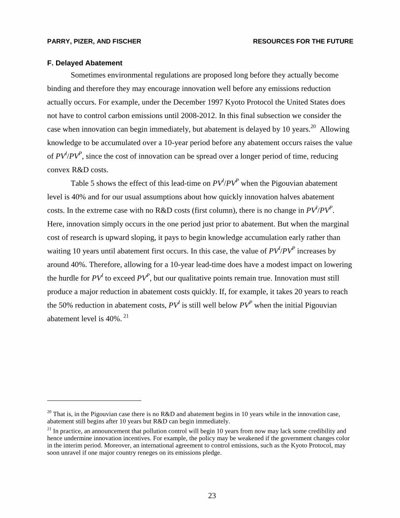
Table 5 shows the effect of this lead-time on PVI/PVP when the Pigouvian abatement

level is 40% and for our usual assumptions about how quickly innovation halves abatement

costs. In the extreme case with no R&D costs (first column), there is no change in PVI/PVP.

Here, innovation simply occurs in the one period just prior to abatement. But when the marginal

cost of research is upward sloping, it pays to begin knowledge accumulation early rather than

waiting 10 years until abatement first occurs. In this case, the value of PVI/PVP increases by

around 40%. Therefore, allowing for a 10-year lead-time does have a modest impact on lowering

the hurdle for PVI to exceed PVP, but our qualitative points remain true. Innovation must still

produce a major reduction in abatement costs quickly. If, for example, it takes 20 years to reach

the 50% reduction in abatement costs, PVI is still well below PVP when the initial Pigouvian

abatement level is 40%. 21

20 That is, in the Pigouvian case there is no R&D and abatement begins in 10 years while in the innovation case,abatement still begins after 10 years but R&D can begin immediately.21 In practice, an announcement that pollution control will begin 10 years from now may lack some credibility andhence undermine innovation incentives. For example, the policy may be weakened if the government changes colorin the interim period. Moreover, an international agreement to control emissions, such as the Kyoto Protocol, maysoon unravel if one major country reneges on its emissions pledge.


24

Table 5: PVI/PVP when Abatement Begins after Ten Years (40% abatement)

Time lag until abatement costs halve

0 10 years 20 years 40 years

Abate Now 4.00 1.07 0.46 0.16

Abate in 10 years 4.00 1.53 0.67 0.22

An important caveat to these results is that the abatement delay must be exogenous and

not delayed in order to give innovation a head start. If one imagines a policymaker deciding

between an early focus on innovation incentives rather than immediate reductions, s/he would

compare the scenario with early innovation to one with immediate abatement and no innovation.

The relative gain to innovation of 1.53 in the above table, however, is measured relative to

Pigouvian gains when abatement begins after ten years. This Pigouvian scenario generates only

60% of the welfare gains associated with an immediate abatement plan (based on ten years of

discounting). Thus the gain of early innovation relative to immediate abatement is only 0.92 =

1.53 x 0.60. Therefore, these results do not in any way suggest that abatement should be delayed

in order to permit innovation.

4. Conclusion

This paper uses a dynamic social planning model to estimate the discounted welfare gains

from innovation that reduces the future costs of pollution abatement. These welfare gains are

expressed relative to the discounted “Pigouvian” welfare gains from correcting the pollution

externality when the state of technology is held fixed over time. In general, we find that the

discounted welfare gains from innovation are unlikely to be as large as the discounted Pigouvian

welfare gains, and they could easily be a lot smaller. The reason is the benefits from innovation

are bounded by the potential reduction in abatement costs and, since R&D is costly, it takes time


25

to accumulate enough knowledge to secure a substantial reduction in abatement costs. We find

that the (discounted) welfare gains from innovation could only exceed the (discounted)

Pigouvian welfare gains if innovation substantially reduces abatement costs in a short period of

time and the initial Pigouvian abatement level is fairly modest. Our results apply for both flow

and stock pollutants, for linear and convex environmental damage functions, and for comparing

innovation and abatement over short and long planning horizons. Very low discount rates and

costless R&D can, however, overturn this conclusion. In sum, our analysis casts some doubt on

the assertion that technological innovation rather than pollution control should be the

overriding factor in the design of environmental policies.

At first glance these results may seem surprising because economists and policymakers

alike have tended to lean on innovation as an important cornerstone of modern environmental

policy, especially with regard to climate change. Why does innovation and “technology policy”

attract such attention? One possibility is that stringent emissions reductions may be politically

difficult when the costs are concentrated in one industry while the benefits are widely diffused.

Incentives for innovation may be more palatable. Also, economists often focus on the cost-

effectiveness of different policies associated with a particular emission target. In a cost-

effectiveness setting, technological innovation offers the seductive possibility that abatement

costs could be eliminated but ignores the magnitude of those costs relative to benefits. In any

case, our results in no way rule out the possibility that the absolute welfare gains from

innovation might be substantial, only that they are probably smaller than the welfare gains from

pollution control over time.

There are some limitations to our analysis that might be useful to relax in future work and

hence our results should be viewed with some caution. For example, we have compared the

welfare gains from the socially optimal amount of innovation to the welfare gains from the

socially optimum amount of pollution control. In practice, environmental policies may not be set

optimally, due to “government failure” or because of extreme uncertainty over the (marginal)

benefits and costs of pollution abatement. It might be fruitful to explore the welfare gains from

innovation in a setting when pollution control is sub-optimal.

We also focus only on the first-best welfare gains from pollution control and innovation,

while in practice policy is conducted in a second-best setting. In particular, recent research has


26

shown that the welfare gains from certain pollution control policies can be greatly reduced by

their impact on raising product prices, reducing real factor returns, and consequently

compounding distortions from pre-existing taxes in factor markets (e.g., Goulder et al. (1999)).

The impact of innovation-promoting policies on pre-existing tax distortions has not yet been

estimated in the literature. In fact, it is possible that such policies may reduce the efficiency costs

of pre-existing taxes to the extent that investment in R&D comes at the expense of consumption

rather than investment in other activities. This is because, due to taxes on the income from

investment, investment is “too low” relative to consumption. Consequently, in a second-best

setting the (general equilibrium) welfare gains from increasing innovation may be more

favorable relative to the welfare impacts of pollution control.

On the other hand, due to other second-best considerations, the supply curve of R&D

may understate true opportunity costs. This occurs if environmentally focused R&D crowds out

other (commercial) R&D, and the social rate of return on this R&D exceeds the private rate of

return due to spillovers from knowledge (e.g., Nordhaus, 1998). In this regard then, our results

may overstate the welfare gains from innovation.

Another limitation is that we ignore possible spillover benefits of new abatement

technologies to other industries. If these spillover benefits are environmental for example a

new technique for reducing carbon emissions by using more natural gas can also reduce sulfur

emissions they can raise the overall social benefits from innovation. If the spillover benefits are

economic however, for example the private cost savings from reduced fuel requirements, they

may already be internalized to some extent, prior to the introduction of an environmental policy.


27

References

Burtraw, Dallas, 1996. “The SO2 Emissions Trading Program: Cost Savings Without

Allowance Trades.” Contemporary Economic Policy XIV: 79-94.

Burtraw, Dallas, Alan J. Krupnick, Erin Mansur, David Austin and Deirdre Farrell, 1997.

“The Costs and Benefits of Reducing Acid Rain.” Discussion paper No. 97-31, Resources for the

Future, Washington, D.C.

Cropper, Maureen L. and Wallace E. Oates, 1992. “Environmental Economics: A

Survey.” Journal of Economic Literature XXX: 675-740.

Fischer, Carolyn, Ian W.H. Parry and William A. Pizer, 1999. “Instrument Choice for

Environmental Protection when Technological Innovation is Endogenous.” Discussion paper,

Resources for the Future, Washington, D.C.

EIA, 1999. Annual Energy Outlook 2000 (December). Energy Information

Administration, US Department of Energy, Washington, D.C.

Goulder, Lawrence H. and Koshy Mathai, 2000. “Optimal CO2 Abatement in the

Presence of Induced Technological Change.” Journal of Environmental Economics and

Management 3: 1-38.

Goulder, Lawrence H., Ian W.H. Parry, Roberton C. Williams and Dallas Burtraw, 1999.

“The Cost-Effectiveness of Alternative Instruments for Environmental Protection in a Second-

Best Setting.” Journal of Public Economics 72: 329-360.

Hahn, Robert W. and Robert N. Stavins, 1992. “Economics Incentives for Environmental

Protection: Integrating Theory and Practice,” American Economic Review Papers and

Proceedings 82(2), p. 464-468.


28

Hammitt, James, K., 1997. “Stratospheric-Ozone Depletion.” In Richard D. Morgenstern

(ed.), Economic Analyses at EPA: Assessing Regulatory Impact, Resources for the Future,

Washington, D.C.

Jung, Chulho, Kerry Krutilla and Roy Boyd, 1996. “Incentives for Advanced Pollution

Abatement Technology at the Industry Level: An Evaluation of Policy Alternatives.” Journal of

Environmental Economics and Management 30, 95–111.

Kneese, Allen V. and Charles L. Schultz, 1978. Pollution, Prices and Public Policy.

Brookings Institute, Washington, DC.

Milliman, Scott, R. and Raymond Prince, 1989. “Firm Incentives to Promote

Technological Change in Pollution Control.” Journal of Environmental Economics and

Management 17, 247−65.

Newell, Richard G. and Robert N. Stavins, 2000. “Abatement-Cost Heterogeneity and

Anticipated Savings from Market-Based Environmental Policies.” Working Paper, Resources for

the Future, Washington, D.C.

Nichols, Albert, L., 1997. “Lead in Gasoline.” In Richard D. Morgenstern (ed.),

Economic Analyses at EPA: Assessing Regulatory Impact, Resources for the Future,

Washington, D.C.

Nordhaus, William, D., 1998. “Modeling Induced Innovation in Climate-Change Policy.”

Discussion paper, Yale University, New Haven, Conn.

Nordhaus, William, D., 1994. Managing the Global Commons. The Economics of

Climate Change. MIT Press; Cambridge, Mass.


29

Orr, Lloyd, 1976. “Incentive for Innovation as the Basis for Effluent Charge Strategy.”

American Economic Review 66:441-447.

Parry, Ian W.H., 1998. “Pollution Regulation and the Efficiency Gains from

Technological Innovation.” Journal of Regulatory Economics 14: 229-254.

Parry, Ian W.H., 1995. “Optimal Pollution Taxes and Endogenous Technological

Progress.” Resource and Energy Economics 17, 69−85.

Portney, Paul, 1999. “The Joy of Flexibility: U.S. Climate Policy in the Next Decade.”

Address to the National Energy Modeling System/Annual Outlook Conference, U.S. Energy

InformationAdministration, March. Available at www.weathervane.rff.org/refdocs

/portney_flex.pdf.

Portney, Paul and John P. Weyant, 1999. Discounting and Intergenerational Equity.

Resources for the Future, Washington D.C.

http://www.weathervane.rff.org/

How Important is Technological Innovation in Protecting the Environment?

Documents

Transcript of How Important is Technological Innovation in Protecting the Environment?