http://pih.sagepub.com/Medicine

Engineers, Part H: Journal of Engineering in Proceedings of the Institution of Mechanical

http://pih.sagepub.com/content/224/3/487The online version of this article can be found at:

 DOI: 10.1243/09544119JEIM668

2010 224: 487Proceedings of the Institution of Mechanical Engineers, Part H: Journal of Engineering in MedicineE Rashedi, K Khalaf, M Reza Nassajian, B Nasseroleslami and M Parnianpour

L5 level−−Three-dimensional isometric exertions with 18 Hill-model-based muscle fascicles at the L4How does the central nervous system address the kinetic redundancy in the lumbar spine?

  

Published by:

http://www.sagepublications.com

On behalf of: 

  Institution of Mechanical Engineers

can be found at:Proceedings of the Institution of Mechanical Engineers, Part H: Journal of Engineering in MedicineAdditional services and information for

   

  http://pih.sagepub.com/cgi/alertsEmail Alerts:

 

http://pih.sagepub.com/subscriptionsSubscriptions:  

http://www.sagepub.com/journalsReprints.navReprints:  

http://www.sagepub.com/journalsPermissions.navPermissions:  

http://pih.sagepub.com/content/224/3/487.refs.htmlCitations:  

What is This? 

- Mar 1, 2010Version of Record >>

at Virginia Tech on June 26, 2013pih.sagepub.comDownloaded from

How does the central nervous system address the kineticredundancy in the lumbar spine? Three-dimensionalisometric exertions with 18 Hill-model-based musclefascicles at the L4–L5 levelE Rashedi1*, K Khalaf2, M Reza Nassajian1, B Nasseroleslami3, and M Parnianpour1,4

1School of Mechanical Engineering, Sharif University of Technology, Tehran, Iran2Department of Mechanical Engineering, American University of Shadjeh, Sharjeh, United Arab Emirates3Bioengineering Unit, University of Strathclyde, Glasgow, UK4Department of Information and Industrial Engineering, Hanyang University, Ansan, Gyeonggi-do, Republic of Korea

The manuscript was received on 30 May 2009 and was accepted after revision for publication on 16 September 2009.

DOI: 10.1243/09544119JEIM668

Abstract: The human motor system is organized for execution of various motor tasks in adifferent and flexible manner. The kinetic redundancy in the human musculoskeletal system isa significant property by which the central nervous system achieves many complementarygoals. An equilibrium-based biomechanical model of isometric three-dimensional exertions oftrunk muscles has been developed. Following the definition and role of the uncontrolledmanifold, the kinetic redundancy concept is explored in mathematical terms. The null space ofthe kinetically redundant system when a certain joint moment and/or stiffness are needed isderived and discussed. The aforementioned concepts have been illustrated, using a three-dimensional three-degrees-of-freedom biomechanical model of the spine with 18 anatomicallyoriented Hill-type-model muscle fascicles. The considerations of stability and its consequenceon the internal loading of the spine and coactivation consequences are discussed in bothgeneral and specific cases. The results can shed light on the interaction mechanisms in muscleactivation patterns seen in various tasks and exertions and can provide a significantunderstanding for future research studies and clinical practices related to low-back disorders.Alteration of recruitment patterns in low-back-pain patients has been explained on the basis ofthis biomechanical analysis. The higher coactivation results in higher internal loading whileproviding higher joint stiffness that enhances spinal stability, which guards against spinaldeformation in the presence of any perturbations.

Keywords: central nervous system, kinetic redundancy, lumbar spine, biomechanical model,Hill-model-based muscle fascicles

1 INTRODUCTION

In order to evaluate the loads acting on interverteb-

ral joints in the spine to prevent injuries from

overloading, the muscle forces should be deter-

mined. While in-vivo muscle forces are not measur-

able non-invasively, using mathematical models to

estimate these forces is unavoidable. The challenge

of predicting the muscle recruitment patterns for

maintaining biomechanical balance in the trunk is

due to redundancy in the neuromusculoskeletal

system, and how the central nervous system (CNS)

manages this problem is ill understood. There are

three approaches to addressing this issue: using

optimization methods [1, 2], electromyography

(EMG)-driven models [3], and kinematic-based finite

element models [4]. In the study by Pomero et al. [5],

which utilized some similar formulae to the math-

ematical equations in this paper, a model is used

*Corresponding author: Biomechanics Laboratory, School of

Mechanical Engineering, Sharif University of Technology, Azadi

Avenue, Tehran, Iran.

email: ehsan.rashedi@gmail.com

487

JEIM668 Proc. IMechE Vol. 224 Part H: J. Engineering in Medicine

at Virginia Tech on June 26, 2013pih.sagepub.comDownloaded from

which avoided spinal joint overloading by maintain-

ing spine loads within proper bounds of its tolerance

limits, while considering a predetermined schema

for muscle coactivations.

Kinetic redundancy in the human musculoskeletal

system gives considerable advantages, as it provides

greater methods of achieving a requested task by the

CNS. From a computational standpoint this is

usually a mathematical challenge to describe how

these extra degrees of freedom are managed for a

single task (which usually means how the internal

muscle forces are specified to balance the external

moments while satisfying the equilibrium condi-

tions) [7]. For simple joints with a pair of agonist and

antagonist muscles, antagonistic activation can be

discussed qualitatively from experimental data, and

quantitative analysis requires biomechanical models

[2]. However, for complex joints with multiple

muscles, there is difficulty even in assigning qualita-

tively the role of synergistic and antagonistic action

to muscles [2, 8]. In practice, there are many other

objectives associated with each task besides main-

taining equilibrium, such as the required accuracy,

stiffness, and necessary adaptation to muscular

fatigue among others [1].

An integrated mathematical description for simul-

taneous force and stiffness control of a joint is

explained and relevant considerations about the

controlled and uncontrolled biomechanical para-

meters are discussed after the introductory explana-

tion of synergistic muscles actions, force generation,

and stiffness formulation of the trunk are derived.

The solution for a redundant system of equations is

obtained by optimization, while the redundancy

concept is explained by the null space of the system

of equations and the uncontrolled manifold. This

approach gives computational advantages compared

with the EMG-driven model, as it does not restrict

the domain of results to a few experimentally

observed patterns and allows classification of results

based on the theoretically defined concepts and

parameters. The possibility of comparing the results

of simulating various objective functions allows

further understanding of the normal and abnormal

patterns of trunk muscle recruitments (i.e. higher

coactivation by low-back patients). The solutions for

a simplified trunk model are used as illustrative

examples in three different tasks and specified

strategies. The generated moment, trunk stiffness,

and joint reaction forces are compared for these

three cases.

2 METHODS

2.1 Force equilibrium

A free-body diagram including all relevant muscles

could be analysed to give the mathematical relation-

ship of the equilibrium condition. All physiological

and geometrical properties such as the line of action

and cross-sectional area of the muscles will be

considered (Table 1 [5, 9]). The convention sug-

gested by the International Society of Biomechanics

is followed to describe the spine’s coordinate system

[10]. The y axis is the line passing through the

centres of the vertebra’s upper and lower end plates,

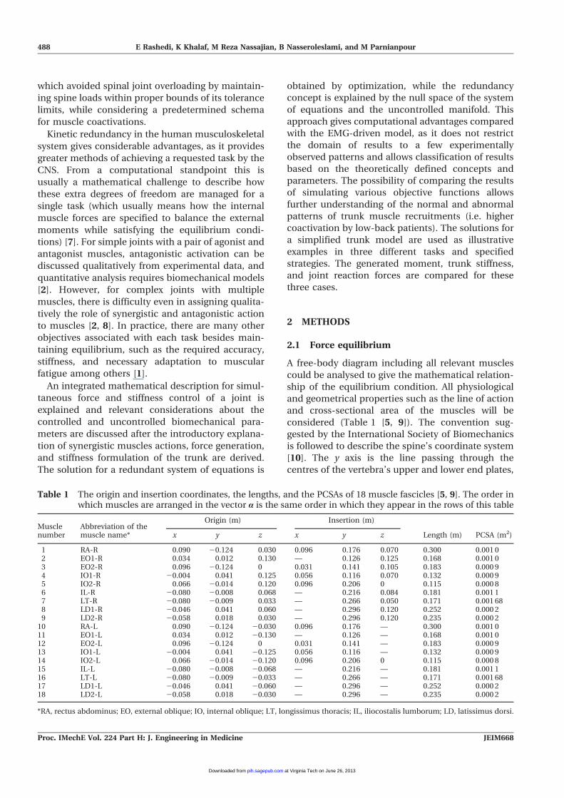
Table 1 The origin and insertion coordinates, the lengths, and the PCSAs of 18 muscle fascicles [5, 9]. The order inwhich muscles are arranged in the vector a is the same order in which they appear in the rows of this table

Musclenumber

Abbreviation of themuscle name*

Origin (m) Insertion (m)

Length (m) PCSA (m2)x y z x y z

1 RA-R 0.090 20.124 0.030 0.096 0.176 0.070 0.300 0.001 02 EO1-R 0.034 0.012 0.130 — 0.126 0.125 0.168 0.001 03 EO2-R 0.096 20.124 0 0.031 0.141 0.105 0.183 0.000 94 IO1-R 20.004 0.041 0.125 0.056 0.116 0.070 0.132 0.000 95 IO2-R 0.066 20.014 0.120 0.096 0.206 0 0.115 0.000 86 IL-R 20.080 20.008 0.068 — 0.216 0.084 0.181 0.001 17 LT-R 20.080 20.009 0.033 — 0.266 0.050 0.171 0.001 688 LD1-R 20.046 0.041 0.060 — 0.296 0.120 0.252 0.000 29 LD2-R 20.058 0.018 0.030 — 0.296 0.120 0.235 0.000 2

10 RA-L 0.090 20.124 20.030 0.096 0.176 — 0.300 0.001 011 EO1-L 0.034 0.012 20.130 — 0.126 — 0.168 0.001 012 EO2-L 0.096 20.124 0 0.031 0.141 — 0.183 0.000 913 IO1-L 20.004 0.041 20.125 0.056 0.116 — 0.132 0.000 914 IO2-L 0.066 20.014 20.120 0.096 0.206 0 0.115 0.000 815 IL-L 20.080 20.008 20.068 — 0.216 — 0.181 0.001 116 LT-L 20.080 20.009 20.033 — 0.266 — 0.171 0.001 6817 LD1-L 20.046 0.041 20.060 — 0.296 — 0.252 0.000 218 LD2-L 20.058 0.018 20.030 — 0.296 — 0.235 0.000 2

*RA, rectus abdominus; EO, external oblique; IO, internal oblique; LT, longissimus thoracis; IL, iliocostalis lumborum; LD, latissimus dorsi.

488 E Rashedi, K Khalaf, M Reza Nassajian, B Nasseroleslami, and M Parnianpour

Proc. IMechE Vol. 224 Part H: J. Engineering in Medicine JEIM668

at Virginia Tech on June 26, 2013pih.sagepub.comDownloaded from

and pointing to the cephalad. The z axis is the line

parallel to a line joining similar landmarks on the

bases of the right and left pedicles, and pointing to

the right. Finally, the x axis is the line perpendicular

to the y and z axes, and pointing anteriorly. The

present model studies isometric exertions and/or

efforts in the upright standing position, while the

model structure is general and can address dynamic

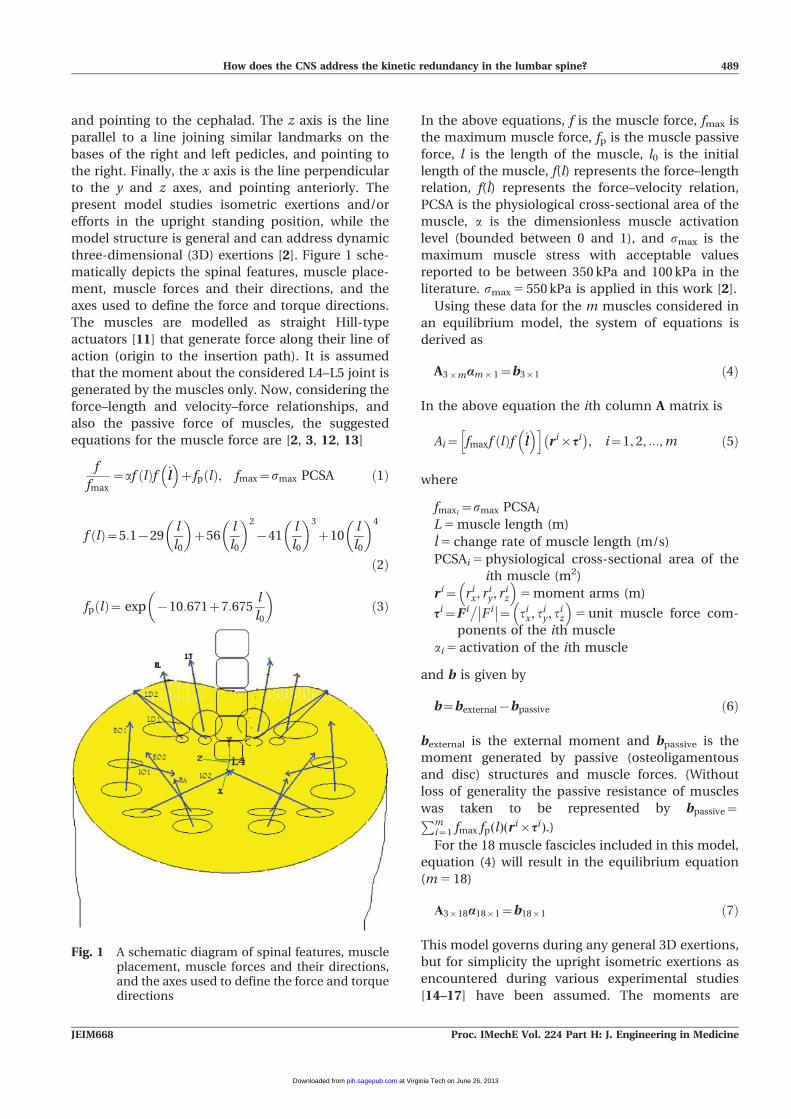
three-dimensional (3D) exertions [2]. Figure 1 sche-

matically depicts the spinal features, muscle place-

ment, muscle forces and their directions, and the

axes used to define the force and torque directions.

The muscles are modelled as straight Hill-type

actuators [11] that generate force along their line of

action (origin to the insertion path). It is assumed

that the moment about the considered L4–L5 joint is

generated by the muscles only. Now, considering the

force–length and velocity–force relationships, and

also the passive force of muscles, the suggested

equations for the muscle force are [2, 3, 12, 13]

f

fmax~af lð Þf _ll

� �zfp lð Þ, fmax~smax PCSA ð1Þ

f lð Þ~5:1{29l

l0

� �z56

l

l0

� �2

{41l

l0

� �3

z10l

l0

� �4

ð2Þ

fp lð Þ~ exp {10:671z7:675l

l0

� �ð3Þ

In the above equations, f is the muscle force, fmax is

the maximum muscle force, fp is the muscle passive

force, l is the length of the muscle, l0 is the initial

length of the muscle, f(l) represents the force–length

relation, f(l̇) represents the force–velocity relation,

PCSA is the physiological cross-sectional area of the

muscle, a is the dimensionless muscle activation

level (bounded between 0 and 1), and smax is the

maximum muscle stress with acceptable values

reported to be between 350 kPa and 100 kPa in the

literature. smax5 550 kPa is applied in this work [2].

Using these data for the m muscles considered in

an equilibrium model, the system of equations is

derived as

A3|mam|1~b3|1 ð4Þ

In the above equation the ith column A matrix is

Ai~ fmaxf lð Þf _ll� �h i

ri|ti� �

, i~1, 2, :::,m ð5Þ

where

fmaxi~smax PCSAi

L5muscle length (m)

l̇5 change rate of muscle length (m/s)

PCSAi5physiological cross-sectional area of the

ith muscle (m2)

ri~ rix, riy, r

iz

� �5moment arms (m)

ti~F i�Fi�� ��~ tix, t

iy, t

iz

� �5unit muscle force com-

ponents of the ith muscle

ai5 activation of the ith muscle

and b is given by

b~bexternal{bpassive ð6Þ

bexternal is the external moment and bpassive is the

moment generated by passive (osteoligamentous

and disc) structures and muscle forces. (Without

loss of generality the passive resistance of muscles

was taken to be represented by bpassive~Pmi~1 fmax fp(l)(r

i|ti).)

For the 18 muscle fascicles included in this model,

equation (4) will result in the equilibrium equation

(m5 18)

A3|18a18|1~b18|1 ð7Þ

This model governs during any general 3D exertions,

but for simplicity the upright isometric exertions as

encountered during various experimental studies

[14–17] have been assumed. The moments are

Fig. 1 A schematic diagram of spinal features, muscleplacement, muscle forces and their directions,and the axes used to define the force and torquedirections

How does the CNS address the kinetic redundancy in the lumbar spine? 489

JEIM668 Proc. IMechE Vol. 224 Part H: J. Engineering in Medicine

at Virginia Tech on June 26, 2013pih.sagepub.comDownloaded from

obtained about the origin of the coordinate system

at the L4–L5 joint.

2.2 Optimization method

To find the muscle activations in equation (7) for a

desired moment, the optimization method is used

with minimization of the norm of the muscle

activations; the cost function is represented in

reference [2] as

f að Þ~minX18i~1

a2i

!ð8Þ

The cost (or objective) function minimizes the sum

of squared muscle activations subject to equality and

inequality constraints of the system. The former

represents the equations of motion or equilibrium

conditions, and the latter are physiological con-

straints to keep possible activations positive and

bounded according to

Aa~b, 0¡ai¡1, i~1, . . . , 18 ð9Þ

The activation levels are determined by the required

moment, and their values are bounded between 0

and 1 [18].

A3618 is the matrix which is computed on the basis

of the physiology and geometry of the muscles about

the L4–L5 joint (i.e. the muscle origin and insertion

points, the muscles’ line of action, the PCSA, the

maximum stress, and other features that are not

considered in this study such as tendon mechanics,

fascicle fibre type, and muscle fibre orientation). It

has three rows and 18 columns. Each row of the A

matrix is a representation of the maximum con-

tributions of muscles for generation of a specific

moment component. Equivalently, each column

represents the magnitude and direction of maximum

moments that the corresponding muscle can con-

tribute.

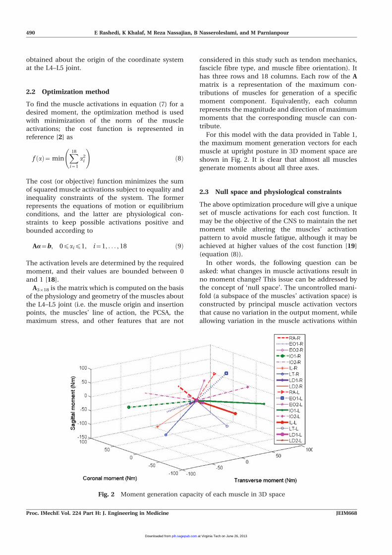
For this model with the data provided in Table 1,

the maximum moment generation vectors for each

muscle at upright posture in 3D moment space are

shown in Fig. 2. It is clear that almost all muscles

generate moments about all three axes.

2.3 Null space and physiological constraints

The above optimization procedure will give a unique

set of muscle activations for each cost function. It

may be the objective of the CNS to maintain the net

moment while altering the muscles’ activation

pattern to avoid muscle fatigue, although it may be

achieved at higher values of the cost function [19]

(equation (8)).

In other words, the following question can be

asked: what changes in muscle activations result in

no moment change? This issue can be addressed by

the concept of ‘null space’. The uncontrolled mani-

fold (a subspace of the muscles’ activation space) is

constructed by principal muscle activation vectors

that cause no variation in the output moment, while

allowing variation in the muscle activations within

Fig. 2 Moment generation capacity of each muscle in 3D space

490 E Rashedi, K Khalaf, M Reza Nassajian, B Nasseroleslami, and M Parnianpour

Proc. IMechE Vol. 224 Part H: J. Engineering in Medicine JEIM668

at Virginia Tech on June 26, 2013pih.sagepub.comDownloaded from

the subspace. Null space depends on just the

physical characteristics of the model, which are

represented in the matrix A. To span the uncon-

trolled manifold, it is necessary solve the set of

equations [20]

A3|18e18|1~0 ð10Þ

This set of homogeneous linear equations can be

considered as a matrix and vector equation; e can be

characterized as a right singular vector correspond-

ing to a zero singular value. A non-negative real

number c is a singular value for A if and only if there

exist unit-length vectors u and u such that

Av~cu ð11Þ

The vectors u and u are called left-singular and right-

singular vectors respectively for c.

Using the singular value decomposition method to

generate the null space, vectors A will be decom-

posed into three matrices according to

A3|18~U3|3S3|18VT18|18 ð12Þ

The diagonal entries of S are necessarily equal to the

singular values of A, with other elements of S equal

to zero. The columns of the matrices U and V are left

and right singular vectors respectively for the

corresponding singular values. The superscript T

indicates the matrix transpose.

There are two subspaces in the muscles’ activation

space which are represented by V: the null space and a

space perpendicular to this null space. Moving along

the unit vectors of the null space results in no change

in the producedmoment, while moving along the unit

vectors of the perpendicular subspace to the null

space results in changes in the produced moment.

The number of vectors in the null space is equal to

the degrees of redundancy in the system. It should

be noted that, as there are three equations with 18

unknowns, the degrees of redundancy will be 15, and

consequently there are 15 unit vectors in the null

space. Each of these vectors in the null space

represents a key direction of the aforementioned

redundancy in the space of the muscle activations.

Because of the physiological constraints (e.g. the

activation range and muscle maximum stress), not

all vectors in the null space may be permissible (i.e.

some directions or values yielding negative muscle

activation or supra-maximal activation). This may

reduce the real degree of redundancy.

To address this issue, it should be noted that using

the optimization method will give a point in the

space of the muscle activations that minimizes the

cost function and satisfies the equilibrium and

physiological constraints (9). This point will be in

an 18-dimensional unit hypercube which covers the

entire workspace here. There are 15 lines that go

through the mentioned point in the directions

provided by the unit vectors of the null space. Only

the sections of the lines inside the workspace

hypercube correspond to feasible results. Any com-

bination of permissible values of muscle activation

can be recruited without any concern about indu-

cing change in the desired moment. To apply this

concept, the required line equation is

x1{a1e1, j

~x2{a2e2, j

~ � � �~ xi{aiei, j

~tj

i~1, . . . ,18, j~1, . . . ,15 ð13Þ

In the above equation, a1, a2,…, a18 are the muscle

activations obtained by the above-mentioned opti-

mization procedure, e1, j, e2, j,…, e18, j are the Cartes-

ian components of the 15 unit vectors ej of the null

space, and x1, x2,…, x18 are the variables in the

muscle activation space. The range of tj determines

the permissible recruitment along the vectors of the

null space without changing the net moments. The

purpose is to find any possible range for the variable

tj which is obtained by considering the boundedness

of independent variables xi to the [0, 1] range. If

there is such a range for tj, any coefficient chosen

from this interval can be multiplied by ej and added

to the activation vector obtained by the optimization

method. Using the same procedure for all the vectors

in the null space will clarify the possibility of

changing the muscle activation in positive activation

space without changing the required moment.

To illustrate these concepts further, the uncon-

trolled manifold computed for the following ex-

ample is plotted in Fig. 3. Suppose that the model

has just the first three muscles to generate the

moment about the L4–L5 level, as mentioned in

Table 1. The CNS goal is to achieve the generation of

a flexion moment of 280Nm in the x direction. In

this case, there is just one equilibrium equation with

three unknown muscle activations, which is

A1|3a3|1j j~{80Nm ð14Þ

Figure 3 shows that various optimal solutions lie on

the uncontrolled manifold surface. It shows that the

choice of optimal solution a* in the construction of

the uncontrolled manifold is irrelevant. In this

example the three cost functions were the minimum

How does the CNS address the kinetic redundancy in the lumbar spine? 491

JEIM668 Proc. IMechE Vol. 224 Part H: J. Engineering in Medicine

at Virginia Tech on June 26, 2013pih.sagepub.comDownloaded from

sum of the muscle stresses, the minimum norm, and

the minimum sum of cubed activations. In short,

points on this surface are all the infinite solutions

that satisfy equilibrium conditions and keep the

muscle activation positive. Any points outside this

manifold violate the equilibrium conditions. The

characteristics of the uncontrolled manifold surface

(its normal vector direction in space) is just

dependent on A163. Different values of the moment

will shift this surface up or down along its normal

vector, but the normal vector of the uncontrolled

manifold surface will remain invariant.

2.4 Angular stiffness

The assumption that the muscle stiffness can be

effectively estimated as a function of muscle force

and length has been well established in spine

stability studies [21, 22]. Some studies have con-

cluded that the muscle stiffness is approximately

linearly proportional to the muscle force [23, 24].

One approach taken to reduce the redundancy is to

add new equations in terms of the same unknowns

(i.e. ai in our case) to the original system of

equations. This can be achieved by adding joint

stiffness equations as functions of the muscle

stiffness to the former model (9). To prepare these

equations, the desired angular joint stiffness is used

to provide three more equations, and the new

system of equations for a general case of m muscles

in the model will be

A3|m

B3|m

am|1~

b3|1

d3|1

ð15Þ

In equation (15) there are six equations and m

unknowns, and so the degree of redundancy for the

system is m2 6, and the null space has m2 6

dimensions. Similar formulae for simultaneous mo-

ment equilibrium and joint reaction force has been

used [25], but not for stiffness.

In the above equation, d361 is the desired triplet of

joint stiffness (Nm/rad). In general, the angular joint

stiffness can be described by

K~

LM1

Lh1LM1

Lh2LM1

Lh3LM2

Lh1LM2

Lh2LM2

Lh3LM3

Lh1LM3

Lh2LM3

Lh3

26666664

37777775

ð16Þ

K is the stiffness matrix of the three-degrees-of-

freedom musculoskeletal system, where, in

Kij5 LMi/Lhj, Mi and hj are the corresponding

moment and joint angle. Suppose that dm63 is the

moment arm matrix and can be described as

d~

Ll1Lh1

Ll1Lh2

Ll1Lh3

Ll2Lh1

Ll2Lh2

Ll2Lh3

Ll3Lh1

Ll3Lh2

Ll3Lh3

..

. ... ..

.

LlmLh1

LlmLh2

LlmLh3

26666666666666664

37777777777777775

ð17Þ

where, in dij5 Lli/Lhj, li and hj are the corresponding

muscle length and joint angle. According to the

Bergmark equation kmm5q(fm/lm) (where kmm is the

linear scalar stiffness of the mth muscle and is given

by kmm5 LFm/Llm)

k~

k11 0 0 � � � 0

0 k22 0 � � � 0

0 0 k33 0

..

. ... P

0 0 0 kmm

266666664

377777775

ð18Þ

The stiffness matrix K of the joint as a function of the

Fig. 3 The uncontrolled manifold and the optimiza-tion results for three cost functions: the mini-mum norm, the minimum sum of musclestresses, and the minimum sum of cubedactivations. In this example, the case of threemuscles acting on a single joint is modelled toallow visual inspection of the results. Hence thematrices involved have the following structure:A163 and a361

492 E Rashedi, K Khalaf, M Reza Nassajian, B Nasseroleslami, and M Parnianpour

Proc. IMechE Vol. 224 Part H: J. Engineering in Medicine JEIM668

at Virginia Tech on June 26, 2013pih.sagepub.comDownloaded from

muscle’s stiffness and geometrical configuration is

given by

Kij~LMi

Lhj~

LP

m Fmdmi

� �Lhj

ð19Þ

where i and j are the indices to describe the stiffnessin the body coordinates system and m is the indexfor the mth muscle (F is the muscle force). Thus

Kij~Pm

LFm

LhjdmizFm

Ldmi

Lhj

� �ð20Þ

Assuming that the second-order term Ldmi

�Lhj5

L2lm�(Lhi Lhj) can be ignored, as the second-order

terms are infinitesimal compared with the first-order

terms, especially in the static case

Kij~Pm

LFm

Lhjdmi~

Pm

kmmdmjdmi ð21Þ

Using the above matrix, K can be defined by

K~dTkd ð22Þ

As a simplified approach, the diagonal elements of

the joint stiffness matrix K are assumed to be the

controlled stiffness elements, denoted by d in

equation (15). These are the dominant components

according to the muscular configuration of the sys-

tem. d can be written as

di~Xmj~1

d2jikjj ð23Þ

which gives the relationship for B in equation (15)

when combined with equations (1) to (4) and the

Bergmark relationship for muscle stiffness. For the

purpose of simulations, the constant q of proportion-

ality in the Bergmark formula is assumed to be q58.

3 RESULTS

3.1 Muscle strength and redundancy

The trunk maximum voluntary capacity or strength

is characterized by a surface in the 3D space of

moments (Fig. 4). Any point outside this strength

surface is infeasible as it would require muscle

activation with a value above 1. Points on the

strength surface mean that at least one of the muscle

activations has reached its maximum value of 1. All

points interior to the surface are feasible and many

recruitments can achieve the required moments.

For example, suppose an external load of 50Nm

pure extension at L4–L5 level is being balanced (i.e.

b~ 0 0 50½ �T as a desired triplet moment). This

triplet moment is in the feasible space of the

muscles, as shown in Fig. 4. It is noteworthy that

Fig. 4 Feasible moment space for the muscles in the model known as the strength limits of themodel in clinical settings

How does the CNS address the kinetic redundancy in the lumbar spine? 493

JEIM668 Proc. IMechE Vol. 224 Part H: J. Engineering in Medicine

at Virginia Tech on June 26, 2013pih.sagepub.comDownloaded from

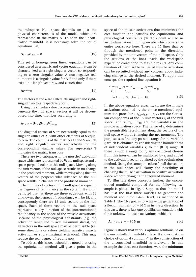
countless different types of muscle activation can

provide this moment. As a solution, the CNS can use

only RA-R and RA-L to produce the desired moment

a~ 0:33 0 0 0 0 0 0 0 0 0:33 0 0½0 0 0 0 0 0 �T

Alternatively, the CNS may use only EO2-R and EO2-L to do the same task (Fig. 5(a)). Using this strategy,the activation vector is

a~ 0 0 0:57 0 0 0 0 0 0 0 0 0:57½0 0 0 0 0 0 �T

The other alternative is to consider simultaneousactivation of all four muscles for the desired resistive

moment (Fig. 5(b)). In this case, one of the manyresultant muscle activations may be

a~ 0:18 0 0:26 0 0 0 0 0 0 0:18 0½0:26 0 0 0 0 0 0 �T

Employing the optimization method in equation (9)for various pure and combined resistive momentsusing all 18 muscles the optimal solution has beenobtained (Table 2). The minimum norm solution forbalancing the 50Nm extension moment using allmuscles will be

a~½ 0:20 0:08 0:12 0 0:10 0 0 0 0

0:20 0:08 0:12 0 0:10 0 0 0 0 �T

Fig. 5 Alternative solutions for resisting an extension of 50Nm of extension by either the rectusabdominis (RA) or external oblique (EO) muscles: (a) two different solutions forgenerating the desired moment; (b) an alternative solution for generating the desiredmoment with four muscles

494 E Rashedi, K Khalaf, M Reza Nassajian, B Nasseroleslami, and M Parnianpour

Proc. IMechE Vol. 224 Part H: J. Engineering in Medicine JEIM668

at Virginia Tech on June 26, 2013pih.sagepub.comDownloaded from

Determination of the agonist, synergist, and antago-

nist actions of muscles during complex exertions

requires detailed analytical reasoning. This issue will

be dealt with elsewhere, although preliminary dis-

cussions have been provided by Potvin and Brown

[25], which will be illustrated by an example.

It is emphasized that many muscles are involved

during a task requiring pure axial rotation or during

complex exertions, even though the minimum norm

solution by definition keeps the antagonist activity to

a minimum (Table 2). Any solution with higher

activation levels for the same b must have used

some combination of activations from the null space

which keeps moments invariant but affects the joint

reaction forces and its stiffness.

The joint stiffness could be added to the above

system of equations. In the model considered here,

the maximum stiffness can be approximated by

multiplying B by the maximum muscle activations,

resulting in

dmax~ 2600 566 3828½ �T Nm=rad

An arbitrary triplet joint stiffness can be chosen as

the submaximal desired angular stiffness according

to

d~ 1000 100 1000½ �T Nm=rad

Balancing the 50Nm external extension moment as

in the previous example and maintaining the desired

specified d, the new matrix for muscle activations by

the minimum norm optimization method will be

a~ 0:42 0 0:12 0:05 0:57 0:14 0:37 0:01½0:03 0:66 0:48 0:60 0 0:28 0:21 0:37

0 0 �T

Comparing the following activation with those of the

first row in Table 2, the additional activity levels can

now be observed as coactivation or antagonist acti-

vity that has provided the desired joint stiffness d.

Obtaining the null space of equation (15) as

explained before and using the same procedure to

Table 2 Muscle activations obtained by the minimum norm optimization method for various pure and combinedexertions

Moment type*Mx

{

(Nm)My

{

(Nm)Mz

{

(Nm)

Activation of the following trunk muscles{

RA-R EO1-R EO2-R IO1-R IO2-R IL-R LT-R LD1-R LD2-R

PureE 0 0 50 0.20 0.08 0.12 0 0.10 0 0 0 0F 0 0 250 0 0 0 0.03 0 0.10 0.15 0.01 0.01LB 50 0 0 0 0 0 0 0 0 0 0 0AR 0 50 0 0 0 0 0.35 0.18 0.06 0.11 0.03 0.03

CombinedE-LB 50 0 50 0.14 0 0.08 0 0 0 0 0 0F-LB 50 0 250 0 0 0 0 0 0 0.09 0 0.01E-AR 0 50 50 0.13 0 0 0.31 0.31 0 0 0.01 0.01F-AR 0 50 250 0 0 0 0.39 0.14 0.15 0.24 0.04 0.05LB-AR 50 50 0 0 0 0 0.24 0.08 0 0.06 0.02 0.03E-LB-AR 50 50 50 0.01 0 0 0.14 0.15 0 0 0 0F-LB-AR 50 50 250 0 0 0 0.28 0.04 0.06 0.19 0.03 0.04

Moment type*Mx

{

(Nm)My

{

(Nm)Mz

{

(Nm)

Activation of the following trunk muscles{

RA-L EO1-L EO2-L IO1-L IO2-L IL-L LT-L LD1-L LD2-L

PureE 0 0 50 0.20 0.08 0.12 0 0.10 0 0 0 0F 0 0 250 0 0 0 0.03 0 0.10 0.15 0.01 0.01LB 50 0 0 0.09 0.18 0.07 0.14 0.13 0.10 0.07 0.01 0.05AR 0 50 0 0.04 0.42 0.18 0 0 0.02 0.02 0 0

CombinedE-LB 50 0 50 0.23 0.20 0.15 0.13 0.24 0 0 0 0F-LB 50 0 250 0 0.18 0.02 0.13 0.04 0.22 0.25 0.03 0.02E-AR 0 50 50 0.21 0.36 0.24 0 0 0 0 0 0F-AR 0 50 250 0 0.43 0.14 0 0 0.12 0.17 0 0LB-AR 50 50 0 0.09 0.58 0.23 0 0 0.13 0.12 0 0E-LB-AR 50 50 50 0.26 0.56 0.30 0 0 0 0 0 0F-LB-AR 50 50 250 0.01 0.60 0.20 0 0 0.23 0.26 0.01 0

*F, flexion; E, extension; LB, right lateral bending; AR, left axial rotation.{Mx, lateral bending moment; My, axial rotation moment; Mz, flexion–extension moment.{RA, rectus abdominus; EO, external oblique; IO, internal oblique; LT, longissimus thoracis; IL, iliocostalis lumborum; LD, latissimus dorsi.

How does the CNS address the kinetic redundancy in the lumbar spine? 495

JEIM668 Proc. IMechE Vol. 224 Part H: J. Engineering in Medicine

at Virginia Tech on June 26, 2013pih.sagepub.comDownloaded from

find any common interval for tj from equation (13),

valid intervals for tj, represented by the lower

bounds tl and upper bounds tu, are computed as

t l~ 0 0 0 0 0 0 0 {0:20 {0:20½0 0 0 �

tu~ 0 0 0 0 0 0:50 0 0 0½0 0 0 �

This is a reasonable result, as the angular joint

stiffness provides a situation in which the sixth,

eighth, and ninth vectors of the null space can

change the muscle activations without any effect on

the desired moment while the positive activations

are guaranteed. This concept can be seen by the

following illustrative examples.

The effect of varying the required or demanded

stiffness while balancing an invariant 50Nm exter-

nal flexion moment in the upright position is shown

in Fig. 6. Higher stiffness is provided by higher

muscle activation as expected with all the negative

energy and loading consequences for the joints.

3.2 Simulation of three cases

The concept is further illustrated by a series of

simulations, assuming 18 muscles in the model

identified in Table 1. Three different tasks or

strategies used by the CNS can be assumed:

Case I: The CNS resists a flexion moment of only

50Nm (b~ 0 0 {50½ �T) and is not affected by

the angular stiffness of the joint.

Case II: The CNS goal is to set the angular joint

stiffness of d~ 1000 100 1000½ �T Nm=rad and

does not specify the moments.

Case III: The CNS is required to set both the

resisting moment and the angular stiffness of the

trunk simultaneously with the values specified in

cases I and II.

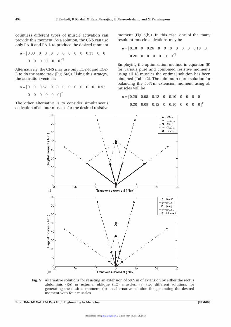
The null space basis vectors tl(i) and tu(i) are

computed accordingly and are presented in Table 3.

In case I, it is expected that different angular

stiffnesses and joint reaction forces will be experi-

enced, although the external moment is not altered,

as the CNS goal is to maintain this desired value

(Fig. 7). It should be noted that, since the muscle

activities dominate the joint reaction forces, the

constant value of body weight has been excluded in

joint reaction forces throughout this paper in all

results. There is one set for t in case I and,

consequently, just the correspondence unit vector

for null space is used in Fig. 7. In case II, all the null

space unit vectors take part in altering the muscle

activations, as can be seen in Table 3. In case III,

Fig. 6 Activations of different muscles for different levels of stiffness demands during thebalancing of a flexion moment of 50Nm (dmax~ 2600 566 3828½ �T Nm=rad)

496 E Rashedi, K Khalaf, M Reza Nassajian, B Nasseroleslami, and M Parnianpour

Proc. IMechE Vol. 224 Part H: J. Engineering in Medicine JEIM668

at Virginia Tech on June 26, 2013pih.sagepub.comDownloaded from

only one of the basis vectors of the null space is

available. In case I, the CNS goal is to generate a

desired value for torque. The results of case II are

interesting since varying t yields large changes in

muscle activations, which affected the generated

torque significantly (Fig. 8(a)). The effects on joint

reaction force were more pronounced when varying

t in this case for some unit vectors of the null space,

i.e. the ninth unit vector (Fig. 8(b)). The last simula-

tion, case III, specified both the joint stiffness and

Table 3 Upper and lower limits of t(i) for the three simulated cases

CNScontrolobjective

Upper and lower limits of the null space basis vector

i5 1 i5 2 i5 3 i5 4 i5 5 i5 6 i5 7 i5 8 i5 9 i5 10 i5 11 i5 12 i5 13 i5 14 i5 15

Case I tl 0 0 0 0 0 0 0 0 0 0 0 0 0 0 0tu 0 0 0 0 0 0 0 0 0 0 0 0 0 0.98 0

Case II tl 20.10 20.40 20.39 20.64 20.02 20.03 20.24 20.40 20.19 20.10 20.40 20.39 20.64 20.02 20.03tu 0.11 0.39 0.70 0.45 0.98 0.98 0.80 0.30 0.83 0.11 0.39 0.70 0.45 0.98 0.98

Case III tl 0 0 0 0 0 0 0 0 0 0 0 0 — — —tu 0 0 0 0 0.34 0 0 0 0 0 0 0 — — —

Fig. 7 Case I: maintaining b~ 0 0 {50½ �T Nm. Variations in (a) the joint stiffness and (b) thejoint reaction forces, as representative parameters of changes in the muscles’ activation(t14) in the uncontrolled manifold

How does the CNS address the kinetic redundancy in the lumbar spine? 497

JEIM668 Proc. IMechE Vol. 224 Part H: J. Engineering in Medicine

at Virginia Tech on June 26, 2013pih.sagepub.comDownloaded from

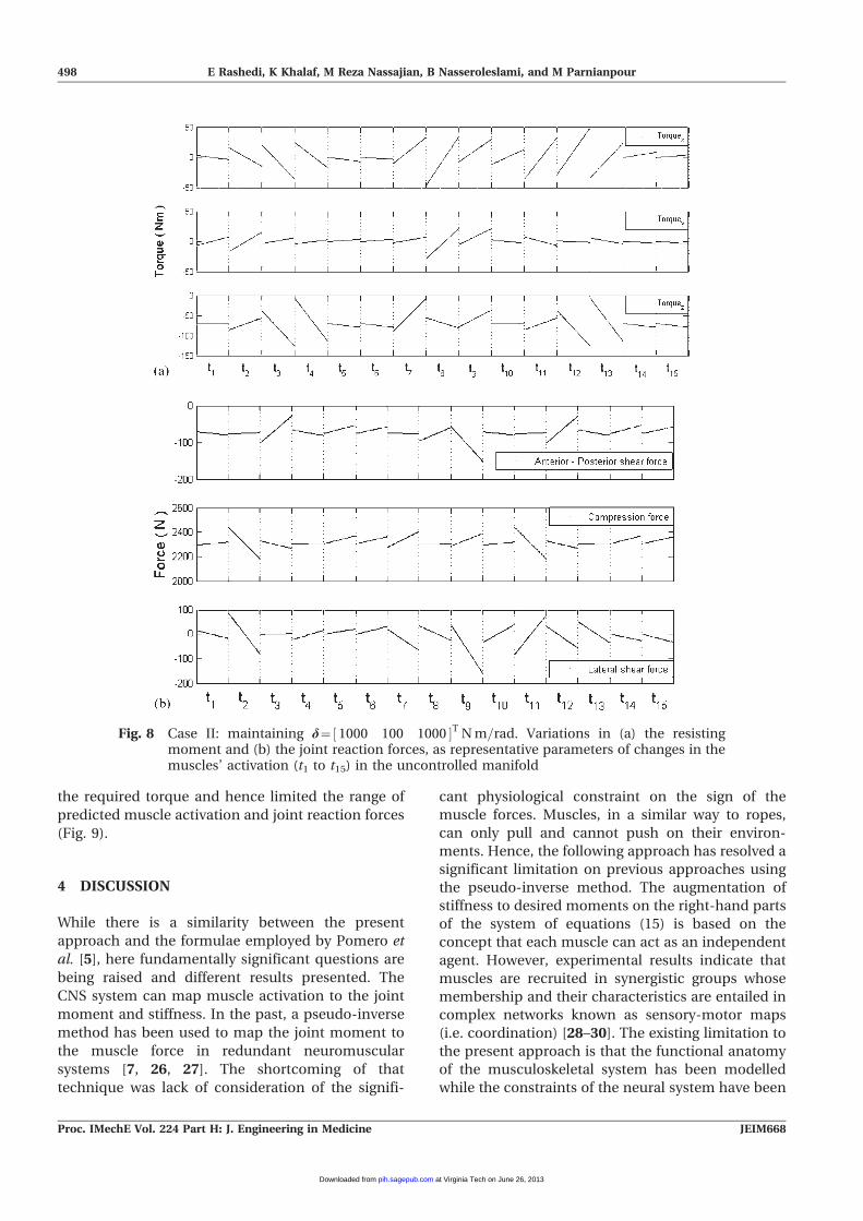
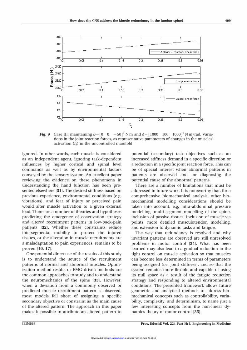
the required torque and hence limited the range of

predicted muscle activation and joint reaction forces

(Fig. 9).

4 DISCUSSION

While there is a similarity between the present

approach and the formulae employed by Pomero et

al. [5], here fundamentally significant questions are

being raised and different results presented. The

CNS system can map muscle activation to the joint

moment and stiffness. In the past, a pseudo-inverse

method has been used to map the joint moment to

the muscle force in redundant neuromuscular

systems [7, 26, 27]. The shortcoming of that

technique was lack of consideration of the signifi-

cant physiological constraint on the sign of the

muscle forces. Muscles, in a similar way to ropes,

can only pull and cannot push on their environ-

ments. Hence, the following approach has resolved a

significant limitation on previous approaches using

the pseudo-inverse method. The augmentation of

stiffness to desired moments on the right-hand parts

of the system of equations (15) is based on the

concept that each muscle can act as an independent

agent. However, experimental results indicate that

muscles are recruited in synergistic groups whose

membership and their characteristics are entailed in

complex networks known as sensory-motor maps

(i.e. coordination) [28–30]. The existing limitation to

the present approach is that the functional anatomy

of the musculoskeletal system has been modelled

while the constraints of the neural system have been

Fig. 8 Case II: maintaining d~ 1000 100 1000½ �T Nm=rad. Variations in (a) the resistingmoment and (b) the joint reaction forces, as representative parameters of changes in themuscles’ activation (t1 to t15) in the uncontrolled manifold

498 E Rashedi, K Khalaf, M Reza Nassajian, B Nasseroleslami, and M Parnianpour

Proc. IMechE Vol. 224 Part H: J. Engineering in Medicine JEIM668

at Virginia Tech on June 26, 2013pih.sagepub.comDownloaded from

ignored. In other words, each muscle is considered

as an independent agent, ignoring task-dependent

influences by higher cortical and spinal level

commands as well as by environmental factors

conveyed by the sensory system. An excellent paper

reviewing the evidence on these phenomena in

understanding the hand function has been pre-

sented elsewhere [31]. The desired stiffness based on

previous experience, environmental conditions (e.g.

vibrations), and fear of injury or perceived pain

would alter muscle activation to a given external

load. There are a number of theories and hypotheses

predicting the emergence of coactivation strategy

and altered recruitment patterns in low-back-pain

patients [32]. Whether these constraints reduce

intersegmental mobility to protect the injured

tissues, or the alteration in muscle recruitments are

a maladaptation to pain experiences, remains to be

proven [16, 17].

One potential direct use of the results of this study

is to understand the source of the recruitment

patterns of normal and abnormal muscles. Optim-

ization method results or EMG-driven methods are

the common approaches to study and to understand

the neuromechanics of the spine [33]. However,

when a deviation from a commonly observed or

predicted muscle recruitment pattern is observed,

most models fall short of assigning a specific

secondary objective or constraint as the main cause

of the altered pattern. The approach in this paper

makes it possible to attribute an altered pattern to

potential (secondary) task objectives such as an

increased stiffness demand in a specific direction or

a reduction in a specific joint reaction force. This can

be of special interest when abnormal patterns in

patients are observed and for diagnosing the

potential cause of the abnormal patterns.

There are a number of limitations that must be

addressed in future work. It is noteworthy that, for a

comprehensive biomechanical analysis, other bio-

mechanical modelling considerations should be

taken into account, e.g. intra-abdominal pressure

modelling, multi-segment modelling of the spine,

inclusion of passive tissues, inclusion of muscle via

points, more detailed musculotendon modelling,

and extension to dynamic tasks and fatigue.

The way that redundancy is resolved and why

invariant patterns are observed are still unresolved

problems in motor control [34]. What has been

learned may also lead to a gradual reduction in the

tight control on muscle activation so that muscles

can become less determined in terms of parameters

being assigned (i.e. joint stiffness), and so that the

system remains more flexible and capable of using

its null space as a result of the fatigue reduction

strategy and responding to altered environmental

conditions. The presented framework allows future

geometric and analytical methods to address bio-

mechanical concepts such as controllability, varia-

bility, complexity, and determinism, to name just a

few interesting concepts from the non-linear dy-

namics theory of motor control [35].

Fig. 9 Case III: maintaining b~ 0 0 {50½ �T Nm and d~ 1000 100 1000½ �T Nm=rad. Varia-tions in the joint reaction forces, as representative parameters of changes in the muscles’activation (t5) in the uncontrolled manifold

How does the CNS address the kinetic redundancy in the lumbar spine? 499

JEIM668 Proc. IMechE Vol. 224 Part H: J. Engineering in Medicine

at Virginia Tech on June 26, 2013pih.sagepub.comDownloaded from

5 CONCLUSIONS

In this study, different ways that the CNS may use

the redundancy in the musculoskeletal system are

discussed and the kinetic redundancy concept has

been explored in a model using 18 muscles at the

L4–L5 level. The null space of the kinetically redun-

dant system when a certain joint moment and/or

stiffness is required is derived and discussed.

The results show that the proposed formulae for

maintaining a constant moment or achieving a

desired trunk stiffness is functional, and the recruit-

ment from the null space of the system affects only

the uncontrolled parameters. This holds for cases

where either only one parameter or both the

moment and the stiffness are controlled. The

changes in uncontrolled parameters (e.g. joint

reaction forces) can range from negligible to con-

siderable, implying the importance and significance

of the redundant degrees of freedom in activation

space (null space). The results emphasize the role of

added controlled parameters for a redundant system

and establish a framework for further analysis of

complex multi-muscle models, together with rel-

evant theoretical and clinical considerations.

F Authors 2010

REFERENCES

1 Li, G., Kaufman, K. R., Chao, E. Y., and Rubash,H. E. Prediction of antagonistic muscle forces usinginverse dynamic optimization during flexion/ex-tension of the knee. Trans. ASME, J. Biomech.Engng, 1999, 121, 316–322.

2 Zeinali-Davarani, S., Hemami, H., Barin, K.,Shirazi-Adl, A., and Parnianpour, M. Dynamicstability of spine using stability-based optimizationand muscle spindle reflex. IEEE Trans. NeuralSystems Rehabil. Engng, 2008, 16, 106–118.

3 Nussbaum, M. A. and Chaffin, D. B. Lumbarmuscle force estimation using a subject-invariant5-parameter EMG-based model. J. Biomech., 1998,31, 667–672.

4 Arjmand, N., Shirazi-Adl, A., and Parnianpour, M.Trunk biomechanics during maximum isometricaxial torque exertions in upright standing. Clin.Biomech. (Bristol, Avon), 2008, 23, 969–978.

5 Pomero, V., Lavaste, F., Imbert, G., and Skalli, W.A proprioception based regulation model to esti-mate the trunk muscle forces. Comput. Meth.Biomech. Biomed. Engng, 2004, 7, 331–338.

6 Burdet, E., Osu, R., Franklin, D. W., Milner, T. E.,and Kawato, M. The central nervous systemstabilizes unstable dynamics by learning optimalimpedance. Nature, 2001, 414, 446–449.

7 Neilson, P. D. and Neilson, M. D. Motor maps andsynergies. Hum. Movement Sci, 2005, 24, 774–797.

8 Nasseroleslami, B., Parnianpour, M., and Mou-savi, S. J. Muscles coactivation in biomechanicalmodels. J. Res. Rehabil. Sci. (Med. Univ. Isfahan),2007, 4, 5–10.

9 Cholewicki, J. and McGill, S. M. Mechanicalstability of the in vivo lumbar spine: implicationsfor injury and chronic low back pain. Clin.Biomech. (Bristol, Avon), 1996, 11, 1–15.

10 Wu, G., Siegler, S., Allard, P., Kirtley, C., Leardini,A., Rosenbaum, D., Whittle, M., D’Lima, D. D.,Cristofolini, L., Witte, H., Schmid, O., and Stokes,I. ISB recommendation on definitions of jointcoordinate system of various joints for the report-ing of human joint motion – Part I: ankle, hip, andspine. International Society of Biomechanics. J.Biomech., 2002, 35, 543–548.

11 Pandy, M. G., Zajac, F. E., Sim, E., and Levine,W. S. An optimal control model for maximum-height human jumping. J. Biomech., 1990, 23,1185–1198.

12 Hatze, H. A myocybernetic control model ofskeletal muscle. Biol. Cybernetcs, 1977, 25, 103–119.

13 McGill, S. M. and Norman, R. W. Partitioning ofthe L4–L5 dynamic moment into disc, ligamentous,and muscular components during lifting. Spine,1986, 11, 666–678.

14 Parnianpour, M., Nordin, M., Kahanovitz, N., andFrankel, V. 1988 Volvo award in biomechanics. Thetriaxial coupling of torque generation of trunkmuscles during isometric exertions and the effectof fatiguing isoinertial movements on the motoroutput and movement patterns. Spine, 1988, 13,982–992.

15 Mousavi, S. J., Olyaei, G. R., Talebian, S., Sanjari,M. A., and Parnianpour, M. The effect of angle andlevel of exertion on trunk neuromuscular perfor-mance during multidirectional isometric activities.Spine, 2009, 34, E170–E177.

16 Moseley, G. L. and Hodges, P. W. Are the changesin postural control associated with low back paincaused by pain interference? Clin. J. Pain, 2005, 21,323–329.

17 Hall, L., Tsao, H., Macdonald, D., Coppieters, M.,and Hodges, P. W. Immediate effects of co-contraction training on motor control of the trunkmuscles in people with recurrent low back pain. J.Electromyogr. Kinesiol., 2009, 19, 763–773.

18 Hughes, R. E., Chaffin, D. B., Lavender, S. A., andAndersson, G. B. J. Evaluation of muscle forceprediction models of the lumbar trunk usingsurface electromyography. J. Orthop. Res., 1994,12, 689–698.

19 Dul, J. The biomechanical prediction of muscleforces. J. Biomech., 1986, 1, 27–28.

20 Scholz, J. P. and Schoner, G. The uncontrolledmanifold concept: identifying control variables fora functional task. Expl Brain Res., 1999, 126,289–306.

500 E Rashedi, K Khalaf, M Reza Nassajian, B Nasseroleslami, and M Parnianpour

Proc. IMechE Vol. 224 Part H: J. Engineering in Medicine JEIM668

at Virginia Tech on June 26, 2013pih.sagepub.comDownloaded from

21 Lawrence, B. M., Buckner, G. D., and Mirka, G. A.An adaptive system identification model of thebiomechanical response of the human trunk dur-ing sudden loading. Trans. ASME, J. Biomech.Engng, 2006, 128, 235–241.

22 Cholewicki, J., Simons, A. P., and Radebold, A.Effects of external trunk loads on lumbar spinestability. J. Biomech., 2000, 33, 1377–1385.

23 Bergmark, A. Stability of the lumbar spine. A studyin mechanical engineering. Acta Orthop. Scand.Suppl., 1989, 230, 1–54.

24 Cholewicki, J. and McGill, S. M. Relationshipbetween muscle force and stiffness in the wholemammalian muscle: a simulation study. Trans.ASME, J. Biomech. Engng, 1995, 117, 339–342.

25 Potvin, J. R. and O’Brien, P. R. Trunk muscle co-contraction increases during fatiguing, isometric,lateral bend exertions. Possible implications forspine stability. Spine, 1998, 23, 774–780; discussion,781.

26 Neilson, M. D. and Neilson, P. D. A neuroengineering solution to optimal tracking problem.Hum. Movement Sci., 1999, 28, 155–183.

27 Yamaguchi, G. T., Moran, D. W., and Si, J. Acomputationally efficient method for solving theredundant problem in biomechanics. J. Biomech.,1995, 28, 999–1005.

28 Ting, L. H. Dimensional reduction in sensorimotorsystems: a framework for understanding musclecoordination of posture. Prog. Brain Res., 2007,165, 299–321.

29 Ting, L. H. and McKay, J. L. Neuromechanics ofmuscle synergies for posture and movement. Curr.Opinion Neurobiol., 2007, 17, 622–628.

30 Scott, S. H. Optimal feedback control and theneural basis of volitional motor control. NatureRev. Neurosci., 2004, 5, 532–546.

31 Schieber, M. H. and Santello, M. Hand function:peripheral and central constraints on performance.J. Appl. Physiol., 2004, 96, 2293–2300.

32 Van Dieen, J. H., Selen, L. P., and Cholewicki, J.Trunk muscle activation in low-back pain patients,an analysis of the literature. J. Electromyogr.Kinesiol., 2003, 13, 333–351.

33 Reeves, N. P. and Cholewicki, J. Modeling thehuman lumbar spine for assessing spinal loads,stability, and risk of injury. Crit. Rev. Biomed.Engng, 2003, 31, 73–139.

34 Guigon, E., Baraduc, P., and Desmurget, M.Computational motor control: redundancy andinvariance. J. Neurophysiol., 2007, 97, 331–347.

35 Riley, M. A. and Turvey, M. T. Variability ofdeterminism in motor behavior. J. Mot. Behav.,2002, 34, 99–125.

How does the CNS address the kinetic redundancy in the lumbar spine? 501

JEIM668 Proc. IMechE Vol. 224 Part H: J. Engineering in Medicine

at Virginia Tech on June 26, 2013pih.sagepub.comDownloaded from