How Does Pension Reform Affect Savings and Welfare

Banco Central de ChileDocumentos de Trabajo

Central Bank of ChileWorking Papers

N° 80

Octubre 2000

HOW DOES PENSION REFORM AFFECTSAVINGS AND WELFARE

Rodrigo Cifuentes

La serie de Documentos de Trabajo en versión PDF puede obtenerse gratis en la dirección electrónica:http://www.bcentral.cl/Estudios/DTBC/doctrab.htm. Existe la posibilidad de solicitar una copiaimpresa con un costo de $500 si es dentro de Chile y US$12 si es para fuera de Chile. Las solicitudes sepueden hacer por fax: (56-2) 6702231 o a través de correo electrónico: [email protected]

Working Papers in PDF format can be downloaded free of charge from:http://www.bcentral.cl/Estudios/DTBC/doctrab.htm. Hard copy versions can be ordered individuallyfor US$12 per copy (for orders inside Chile the charge is Ch$500.) Orders can be placed by fax: (56-2)6702231 or email: [email protected]

BANCO CENTRAL DE CHILE

CENTRAL BANK OF CHILE

La serie Documentos de Trabajo es una publicación del Banco Central de Chile que divulgalos trabajos de investigación económica realizados por profesionales de esta institución oencargados por ella a terceros. El objetivo de la serie es aportar al debate de tópicosrelevantes y presentar nuevos enfoques en el análisis de los mismos. La difusión de losDocumentos de Trabajo sólo intenta facilitar el intercambio de ideas y dar a conocerinvestigaciones, con carácter preliminar, para su discusión y comentarios.

La publicación de los Documentos de Trabajo no está sujeta a la aprobación previa de losmiembros del Consejo del Banco Central de Chile. Tanto el contenido de los Documentosde Trabajo, como también los análisis y conclusiones que de ellos se deriven, son deexclusiva responsabilidad de su(s) autor(es) y no reflejan necesariamente la opinión delBanco Central de Chile o de sus Consejeros.

The Working Papers series of the Central Bank of Chile disseminates economic researchconducted by Central Bank staff or third parties under the sponsorship of the Bank. Thepurpose of the series is to contribute to the discussion of relevant issues and develop newanalytical or empirical approaches in their analysis. The only aim of the Working Papers isto disseminate preliminary research for its discussion and comments.

Publication of Working Papers is not subject to previous approval by the members of theBoard of the Central Bank. The views and conclusions presented in the papers areexclusively those of the author(s) and do not necessarily reflect the position of the CentralBank of Chile or of the Board members.

Documentos de Trabajo del Banco Central de ChileWorking Papers of the Central Bank of Chile

Huérfanos 1175, primer piso.Teléfono: (56-2) 6702475 Fax: (56-2) 6702231

Documentos de Trabajo Working PaperN° 80 N° 80

HOW DOES PENSION REFORM AFFECTSAVINGS AND WELFARE

Rodrigo CifuentesEconomista Senior

Gerencia de Análisis FinancieroBanco Central de Chile

ResumenEste trabajo estudia los efectos de una reforma de pensiones sobre el ahorro por precaución, laacumulación de riqueza y el bienestar. Se utilizan técnicas de programación dinámica para resolverel consumo óptimo de un trabajador que enfrenta incertidumbre en el ingreso del trabajo y en suspensiones. Luego, con valores de parámetros representativos de EE.UU., se evalúa el impacto sobretrabajadores con distinto nivel de educación de dos políticas. La primera es la eliminación de laredistribución en la fórmula de beneficios actual. La segunda es el cambio de un sistema definidoen beneficios (DB) por uno definido en contribuciones (DC). En el primer caso, los resultadosmuestran que la redistribución es valorada por todos los tipos de trabajadores, incluso los de mayoringreso esperado que esperan pérdidas por la redistribución. El ahorro agregado aumenta en 4%como consecuencia de la mayor incertidumbre. La segunda política tiene las consecuenciascontrarias. El bienestar aumenta al introducir un sistema DC ya que éste cuenta con propiedades deseguro superiores. Estas provienen del hecho de que los períodos con menor varianza en losingresos tienen una mayor ponderación en el cálculo de los beneficios. El ahorro por precaucióndisminuye, con lo que el ahorro agregado cae en 1,4%.

AbstractThis paper explores the effects of pension reform on precautionary savings, wealth accumulationand welfare. The impact of pension programs on income uncertainty through life has been largelyignored in the literature of precautionary savings and pension reform. This paper uses dynamicprogramming techniques to solve for the optimal consumption of a worker that faces uncertainty onlabor and retirement income. Subsequently, with parameter values for the U.S., I study the impactof two policies on workers with different on educational levels. One is the elimination ofredistribution in the current benefits formula. The second is the change from system defined inbenefits (DB) to one defined in contributions (DC). In the first case, results show that redistributionis valued positively by all types of agents, even by those who expect losses from it, given theirexpected income. As a consequence, workers increase their savings to prepare for the increaseduncertainty. The increase in aggregate savings is in the order of 4%. The second case has theopposite consequences. Welfare increases with the adoption of the DC system because it hassuperior insurance properties. The advantage consists in that periods on which the variance ofincome is lower receive a higher weight in the calculation of benefits. Precautionary savings arereduced with a fall in aggregate savings of 1.4%.______________________I am grateful to Robert Barro, David Cutler, Peter Diamond, Martin Feldstein, Chris Foote, David Laibson,Alejandro Micco, David Weil, David Wise and the participants at presentations at Harvard University and theCentral Bank of Chile for their comments and suggestions. I gratefully acknowledge financial support fromthe Central Bank of Chile, The World Bank Graduate Scholarship Program and NBER. Email:[email protected] .

3

1. Introduction

An aging population and systemic maturity have brought much discussion about reforming the

old-age pensions component of Social Security Systems in recent years. The amount of resources

involved in this program in both developed and developing countries make this question an issue of first

order importance in policy analysis. A central component of the debate on reforming social security is the

advantages and disadvantages of moving towards a system defined in contributions (DC) with pre-

funding of benefits. Advocates of this reform claim that a funded DC scheme will provide benefits such

as an increase in aggregate private savings1, reduced distortions in labor markets and improved return in

workers’ contributions.

This paper draws attention to two prevalent issues in the discussion. First, the positive impact on

aggregate savings comes from the fact that during the transition towards the new system, a burden is

imposed on some generations in the form of additional taxes or reduced benefits. This burden is a method

of reducing the public debt that is implicit in a pay-as-you-go (PAYG) system. Therefore, the increase in

aggregate savings ultimately comes from the reduction in the implicit debt in the PAYG system. A policy

that reduces public debt with the result of increasing aggregate savings in the economy is always

available, and therefore, the result is not inherent in pension reform2. If pension reform is done in such a

way that promised benefits for all generations are respected and no new taxes are imposed, there is no

increase in aggregate savings (Valdés-Prieto, 1997; Rangel, 1998).

The second issue is that most of the literature ignores a key dimension in the analysis of Social

Insurance systems, which is the quality of the insurance provided by them. Most of the literature studies

the problem in a context without uncertainty, and therefore is unable to provide an assessment of this

dimension.

This paper contributes to the debate on social security reform by analyzing the problem in a

context in which uncertainty is assumed explicitly. The importance of this is twofold. First, when

uncertainty is considered, pension reform will have consequences on aggregate savings even in the case

when promised benefits are paid to all generations and no new taxes are imposed on any generation. This

arises from the fact that changes in the pension system alter the uncertainty that workers face with respect

to their lifetime resources. Considering uncertainty in order to understand savings behavior seems to be

fundamental, as recent empirical findings show (Carroll, 1997). Public pension systems, in turn,

constitute a major source of income for a large fraction of the population in the U.S. Therefore, changes

1 Feldstein and Samwick (1997) find a considerable impact of pension reform on aggregate savings in the case of

the U.S. In their simulations, transition generations pay for the implicit debt in the old system.2 It is true, though, that pension reform allows the possibility of making a policy to reduce public debt to be more

viable politically.

4

in the variance of remaining lifetime resources will change the savings behavior of a worker during her

life, and thus, aggregate savings.

Second, including uncertainty explicitly allows us to assess which type of pension arrangement

provides a better insurance to workers. Specifically, I measure the variance of pensions that a worker

faces under different pension schemes and the impact that this has on her welfare.

This paper studies the effects on welfare and aggregate savings in the economy of a pension

reform. The specific reform studied in this paper is the following. The current defined benefit system

(DB) in the U.S. is replaced by a DC system in such a way that all promised benefits are paid and that no

new taxes are raised to finance the reform. The appendix provides a proof that such a reform is feasible

and that the rate of return in the new DC system has to be same as that implicit in the original DB

system3. The reform is analyzed in two steps. The first step analyzes the elimination of redistribution in

the DB system. The second analyzes the change in the type of system from a DB to a DC.

The analysis is done by comparing steady states in a partial equilibrium model. The specific

reform considered here allows the transition to be characterized straightforwardly from this comparison.

The choice of partial equilibrium is due to computational constraints. Current available computational

capacity would make calculation of a general equilibrium model of this sort extremely costly in terms of

time. The analysis focuses on the impact of idiosyncratic shocks, both transitory and permanent, to labor

income. The extent to which Social Security systems can insure aggregate shocks is studied in Rangel

and Zeckhauser (1999) and Demange and Laroque (1999).

The model presented here takes Social Security as given, that is, it does not arise endogenously

from agents’ optimization. One concern that sometimes arises about these kinds of models is that if there

is not an explicit reason for having a social security system, then welfare analysis of pension reform will

be biased towards the result that any reform that tends to eliminate Social Security will be positive. This

criticism often mixes two different issues. One is a “correct” concern that if the forces that give origin to

Social Security are not present in the analysis, then part of the benefits associated with it are being

omitted from the analysis. I will address this issue in the next paragraph. But the issue is raised

“incorrectly” in other situations. In particular, the absence of endogenously determined Social Security is

raised against some analyses that find large positive benefits from reforming Social Security toward

funded schemes. In several cases, as in Campbell et al (1999) for example, the problem arises from not

considering how the transition costs are going to be financed. When this happens, large benefits from

reform arise, but they hide the fact that in the transition several generations are being made worse off.

Therefore, moves towards eliminating Social Security look good not because its benefits are not being

3 A similar result can be found in Geanakoplos, Mitchell and Skinner (1998).

5

considered, but because a part of the costs are being left out. In this paper the costs of abandoning the

initial PAYG system are explicitly taken into account in the analysis.

With respect to the “correct” concern, two comments can be made. First, among the most

accepted arguments explaining Social Security are intergenerational income redistribution and

paternalism (Diamond, 1977). The former refers to the fact that the origin of Social Security in the U.S. is

linked to the great depression. A decision was made to redistribute income in favor of some generations

particularly damaged by this event at the expense of all future generations. If this is the case then there is

no reason to have endogenously determined social security in the model. The system is simply part of the

environment once the event that caused its creation is in the past, and the way to deal with it is simply by

recognizing the costs and benefits that the system imposes to all generations. The paternalist argument

says that society cares about some people saving too little for retirement when left to their own devices.

Therefore it imposes a forced savings mechanism on the entire population. This can be embedded in the

analysis assuming that there are heterogeneous preferences and that the political system imposes certain

preferences on lifetime consumption in the entire population, as in Cifuentes and Valdés-Prieto (1997). In

the context of the analysis in this paper, modeling a context consistent with paternalism would amount to

adding more cases to the analysis (with different time preferences), but would not change qualitatively

the results obtained.

Finally, as will be clear from the results, one of the contributions made by this paper is precisely

the fact that when labor income uncertainty is introduced into the analysis the result that less social

security is better is radically changed.

The paper is organized as follows. Section Two discusses the sources of uncertainty that affect

the determination of pensions. Section Three presents the model, the parameters chosen, the solution

techniques and the type of results obtained in the simulation. Section Four presents and discusses the

effects on welfare and savings of the elimination of redistribution in the DB system. Section Five

analyzes the effect on welfare and savings of a reform from a DB to a DC system. Section Six concludes.

2. Uncertainty in Pension Systems

A pensions program can be organized in many different ways. Here, I restrict attention to systems

that relate pensions to the history of labor income. Even among these, there are multiple ways in which

retirement benefits can be determined. The following expression summarizes different factors that can

intervene in determining the level of retirement benefits:

∑ ∏= +=

=R

W

RY

Yi

Y

ijjii kRwkbkap ))(()()(

1

(1)

6

where p is the retirement benefit that the worker receives in the form of an annuity. A worker is assumed

to work from age YW to the age of retirement YR. The retirement benefit is determined as a function of a

weighted sum of taxable wages wi 4, where the weights are the factors bi and a gross rate of return Ri,

compounded between the time of the contribution and that of retirement. The variable k indexes different

pension systems.

For example, a DB system that pays a fixed replacement rate over the average taxable wage over

active life will have a equal to the replacement rate, bi equal to 1/(YR-YW+1) and Ri equal to 1. If the

benefit is determined over the average of the last, say, ten years, bi will be zero for i=YW,…,YR-10 and 1/10

for i=YR-9,…,YR. Replacement rate a may also vary with the level of the weighted sum of taxable wages.

A DC system will have bi equal to the contribution rate at each period and Ri equal to the gross return of

the asset where contributions are invested. Coefficient a will be the annuity factor.

The formula makes clear that the effect of different sources of uncertainty varies across different

pension systems. Therefore, systems differ in the variance of expected benefits at the beginning of life

but also during the lifetime. For example, a DB system that averages all periods of active life gives a

higher weight to realizations of labor income, as compared to a DC system. A DC system, in turn,

introduces variability in the rate of return.

The formula also highlights the fact that there are other sources of uncertainty aside from wages

and returns. In a DB system, a, the replacement rate, can be changed by the authority in response to

financial problems. Also, the degree of redistribution can change according to changes in the preferences

of the political majority.

In the same way that systems transmit shocks to income and to rates of returns to the value of

retirement benefits, they can have mechanisms to insure against adverse idiosyncratic shocks. There are

several ways to do this. In a DB system the replacement rate a can be a decreasing function of the

weighted wage average. In a DC scheme, part of the contribution can be accumulated in a shared account

that is used to supplement retirement income up to a certain target level in the case of poor income

realizations.

It should be noted that the analysis here has been done without reference to whether the system is

funded or not. The distinction between DB and DC systems refers to the way a worker accumulates

benefits throughout her lifetime and not to the type of underlying asset that backs the promises.

7

3. The Model and Parameters

3.1 Model

This paper works with a model of consumption under uncertainty with a set up similar to that of

Zeldes (1989) and Carroll (1992). I assume that workers are active between ages 25 and H, an age known

with certainty, at which time they retire. I assume the workers will die with certainty at age D. H and D

vary for different types of workers. Workers supply labor inelastically during their active lives. I assume

that preferences take the standard additively separable expected utility form such that the intertemporal

maximization problem for the worker is:

( ) ( ) ( )∑+=

−+T

tss

tstt

CCuECu

t 1

max β (2)

11

~)(

~.. ++ +−= tttt YCXRXts (3)

where u(.) is an instantaneous utility function, Ct is consumption, β = 1/(1+δ) is the discount factor with

δ the discount rate, Xt is cash-on-hand (income in period t plus financial wealth in the same period), R is

the gross one-period return on savings and Yt is income. The instantaneous utility function is assumed to

be of the Constant Relative Risk Aversion (CRRA) form:

( )ρ

ρ

−=

−

1

)1(CCu (4)

The income process is described by equations (5) through (9):

65,,25~~~

K== tforVPY ttt (5)

82,,6665 K== tforBYt (6)

tttt NPGP~~

1−= (7)

where Pt is the permanent income at age t, Vt is a transitory shock to income, Bt is the retirement benefit,

Gt is the growth factor of permanent income due to age and Nt is a permanent shock to income. The

transitory and permanent shocks to income are assumed to have a lognormal distribution with parameters:

4 Taxable wage is wi=min(total wage, maximum taxable wage).

8

( ) ( )2~

log2

~log

,2/~~

logNN

NN σσ− (8)

( ) ( )2log

2log ,2/~

~log VVNV σσ− (9)

The mean of the lognormal distribution ensures that the mean of N and V are equal to 1, given

that,

[ ] [ ] [ ] 10exp2/2/exp2/exp~ 2

log2log

2loglog1 ==+−=+=+ NNNNtt NE σσσµ

where µ represents the mean of the normal distribution.

Equation (5) says that the retirement benefit is an annuity. Once the uncertainty about the level of

retirement benefits is resolved, its value is certain for the rest of the retirement period. It should be noted

that despite being a certain variable during retirement, it is a random variable before retirement starts.

The moment at which uncertainty about its level is resolved will vary across systems.

The variable Bt is defined as the level of retirement benefit that is known with certainty at time t.

In other words, Bt is the part of the retirement benefit whose determinants have already been realized. In

systems where benefits are determined as a function of the level of income realized, Bt will be the

retirement benefit that the worker will receive if her labor income were to be zero in all remaining

periods until retirement. In this paper I compare two systems: A DB system in which the benefit is

defined as a fraction of the average wage over all active periods, and a DC system in which the benefit is

defined on the basis of the accumulated individual contributions. In the case of the DB system, the

evolution of Bt is described by:

ψ41

),~

min(~ max

1

YYBB tDB

tDB

t += − (10)

where ψ is the replacement rate and Ymax is the maximum taxable wage. In the case of the DC system, the

evolution of Bt is given by:

φθ ))(,~

min(~

1

max1 ∏

+=− +=

RY

tj

SSjt

DCt

DCt RYYBB (11)

9

where θ is the rate of contribution, RSS is the gross return paid by the social security system on the

individual accounts and φ is the annuity factor, i.e. the factor that converts the stock accumulated in the

individual accounts into an annuity. Equation (11) is specific to the case where the return RSS is certain5.

Additionally, I assume explicit borrowing constraints which implies that6:

tX t ∀≥ 0 (12)

An alternative to explicit liquidity constraints is to assume an environment such that consumers

choose never to borrow as a result of their optimization. This will be obtained if there is a positive

probability of labor income being zero in every period, which can be the result of unemployment, for

example7. This, combined with the fact that marginal utility at zero consumption is infinite with a CRRA

utility function leads to the result that consumers will always want to keep a positive stock of net assets in

order to avoid being left without resources in the event of zero labor income. Therefore, they will never

borrow. It should be noted, however, that the logic behind this result lies in the positive probability of

income being zero not only in one period, but in all remaining periods8. Given the presence of formal and

informal insurance mechanisms to secure a minimum consumption floor (i.e. Social Security and family,

respectively), this argument does not seem to provide a better explanation for borrowing constraints than

those arguments that come from the structure of financial markets.

3.2 Parameters

Preferences

Different scenarios are simulated with different values for preference parameters. The chosen

values cover the range estimated in the literature. Lawrance (1991) estimates discount rates with data

from the Panel Study on Income Dynamics (PSID) on consumption using Euler equations. She finds

considerable heterogeneity among income groups, with estimates ranging from 12% for groups with high

5 When return R is not certain, equation (11) becomes: φθ ),

~min()

~1(

~ max1 YYRBB t

SSDCt

DCt ++= −

6 Note that this prevents consuming retirement benefits before retirement. In some cases, available resources late inlife (income plus financial wealth) can be lower than a retirement benefit known with certainty. This will implythat consumption will jump upwards at retirement.

7 This approach is taken by an important faction of the recent literature of consumption under uncertainty, includingZeldes (1989), Carroll (1992, 1997) and Gourinchas and Parker (1997), among others.

8 The argument goes as follows. Given that income can be zero in the last period, the worker will chose to get to thatperiod with some positive amount of savings. Therefore, she does not incur debt in the next to last period.Applying the same reasoning successively to all previous periods implies that it will never be optimal to borrow.

10

levels of labor income to 19% for groups with low labor income. A different approach for estimation has

appeared in recent consumption literature related to the theory of consumption under uncertainty. This

approach consists of simulating profiles of consumption or wealth over the life cycle, and matching them

with those profiles found in the data. Estimates for underlying parameters in preferences (discount rate

and the parameter of risk aversion) are those that generate in simulations the profiles closest to the data.

Estimates obtained under this method are in general highly sensitive to the parameters assumed in the

simulations. Gourinchas and Parker (1997) estimate discount rates that range from 3.3% to 4.3%

according to the level of education. They use data from the Consumers Expenditures Survey (CEX) on

consumption and income. Their estimates are sensitive to assumptions on other parameters, particularly

the interest rate. Their estimates seem to show a discount rate that is one percentage point above the

market interest rate. Carroll and Samwick (1997) use PSID data on consumption and income. Their point

estimates for the discount rate are highly sensitive to other parameters chosen and range from 5% to 14%.

Moreover, confidence intervals are large. Samwick (1997) estimate distributions of the discount rate

using data on wealth from the Survey of Consumer Finances. The median discount rate varies with

assumptions of the parameter of risk aversion, the definition of financial wealth and the initial level of

assets. In most scenarios chosen, the median discount rate is in the range 3%-5%, although in many cases

the median value lies between 7% and 9%. In the absence of a robust estimate of the discount rate, I use a

conservative value of 3% in the simulations.

The coefficient of risk aversion ρ, in turn, takes the values 0.5, 1 and 5. Gourinchas and Parker

(1997) estimate a value for ρ of 0.5. This estimation is lower than what is generally considered a

“reasonable range,” which is between 1 and 5.

Income Process

The income profiles are taken from Hubbard, Skinner and Zeldes (1994) (HSZ henceforth). HSZ

estimate income profiles over the life cycle with PSID data for 1983-1987 for population groups with

three levels of educational attainment: Non-High School (NHS), High School Degree (HS) and College

Degree (COL). Figure 1 shows the income profiles used. This information is summarized in the model

using the level of permanent income at the start of active life, P25, and a vector of growth factors Gt for t=

26, …, L, where L is the last year of active life.

HSZ estimate the variance of income and decompose it on the variance of permanent and

transitory shocks. The model for income that they use is similar to that of this paper (equations (5) and

11

(7)), except that they allow for a coefficient of the persistence of permanent income to be other than one9.

The parameters they obtain are summarized in Table 1:

Table 1: Variance of Permanent and Income Shocks by Educational AttainmentPercentages________________________________________________________________

Education Variance of Variance ofPermanent Shock Transitory Shock

________________________________________________________________

Non-High School 0.033 0.04High School 0.025 0.021College Degree 0.016 0.014________________________________________________________________Source: HSZ, 1994.

Population Composition

The share of workers at each level of educational attainment is obtained from Census data for

1990. Educational Attainment for the population over 25 years of age in 1990 was: 22.4% Non-High

School, 56.3% High-School Degree and 21.3% College Degree (Bureau of the Census, 1992).

Age of Retirement and Expected length of life

The assumed ages of retirement are: 61 years for NHS, 63 years for HS and 65 years for COL

(Laibson et al., 1998). Length of life in the model is set at the population expected length of life at

retirement. These are calculated based on the tables of mortality by educational attainment in Rogot et al

(1992), applying the methodology described in Vital Statistics for the U.S. 1994. This calculation gives us

an expected age of death of 81 years for NHS, 82 years for HS and 83 years for COL.

Interest Rate

The risk-free interest rate is assumed to be 3%.

9 In log form, equation (7) would be pt = gt + γpt-1+nt. The coefficient γ is assumed to be 1 in this paper, while HSZ

estimate it to be between 0.945 and 0.955. Results change slightly when these numbers are considered. A value of

12

3.3 Pensions systems

The initial DB system

The initial scenario closely resembles the current pay-as-you-go system in the U.S. Benefits are

defined over the average lifetime covered wages. The replacement rate (the ratio of the level of the

retirement benefit over the average of covered wages) is a decreasing function of average covered wages.

This means that the replacement rate the system will give a worker with a history of low wages will be

higher than that given to a worker with a history of higher wages. Therefore, the benefit formula is

progressive.

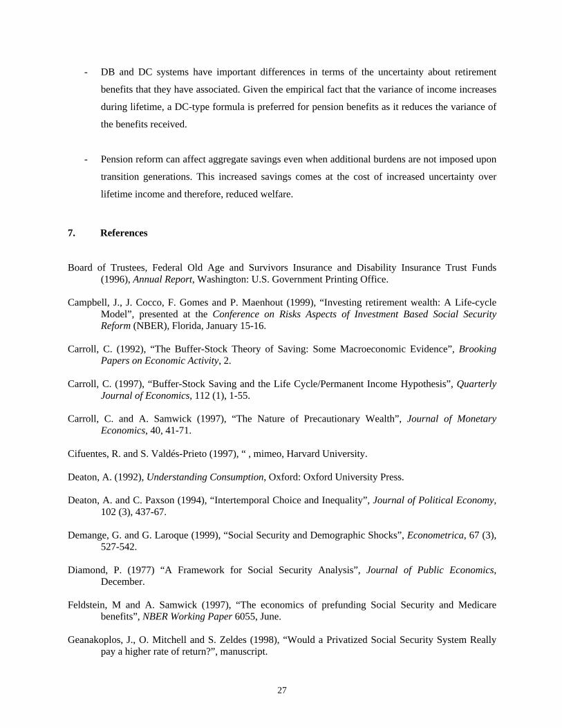
The replacement rate in the model is calculated according to the same formula of benefits as in

the U.S. Social Security system. In terms of equation (10), the replacement rate, ψ, is a function of the

average of taxable wages over active life:

- 90% of the average annual income up to $5112

- An additional 32% of the average annual income in excess of $5112 but below $30,804

- An additional 15% of the average annual income in excess of $30,80410

There is a maximum taxable wage of $61,200 (Social Security Administration, 1997). The

contribution rate is set at 10.6%. Figure 2 shows the benefit formula.

The Internal Rate of Return (IRR) in the DB system

Given the benefit formula described above and the assumptions on the distribution of population,

I then calculate the IRR of the system. This calculation will tell us whether the whole set of demographic

and systemic assumptions provides a good description of the current situation of the pensions system in

the U.S.

To calculate the IRR, I calculate the expected income profile for each type of worker. I run 5,000

histories for each type of worker with their respective income process as described in the previous

section. Using the population weights, I obtain the profile of contributions paid and pensions received

over the lifetime of an average worker. With these payment flows, I can calculate the implicit IRR in the

system, which is the rate of return at which it would be necessary to invest contributions in order to

finance the observed pension benefits. I compare the IRR that I calculate with other calculations in the

literature. Also, the IRR that I calculated must be close to growth of the population and labor productivity

(n+x) during the same years. This is because the IRR is ultimately the return that an unfunded system can

1 is used in this paper for computational simplicity.

10 The cutoff points in the formula (“bend points”) are determined by the Social Security Administration in terms ofmonthly earnings. In monthly terms the cutoff points are $426 and $2567.

13

pay. If the IRR that I calculate is too high in relationship to (n+x) –say above 2.5%-- it would mean the

parameterization that I chose is unrealistic, and that the system is paying benefits that are too high. On

the other side, if the IRR is too low –say, below 0.5%-- it would mean that I have modeled a system that

gives too little benefits.

The IRR that I estimate is 1.72%. Leimer (1994), in a model with a lot more demographic detail,

estimates the IRR to be 1.73% for the cohort born in 1995 and 1.71% for the cohort born in 2050, with

the IRR falling slowly for the cohorts in between. This means that the chosen parameterization provides a

description consistent with reality. With respect to the growth of population and productivity, figures

from the Board of Trustees (1996) show that the geometric average for (n+x) in the period 1990-95 was

1.41%. Considering the cyclical factors that are affecting these realizations, projections for the following

years from the Board of Trustees start at a level of 2.2%. In the intermediate scenario, this figure goes

down steadily, driven basically by decreases in the growth rate of the labor force. The IRR would reach a

level of 1.3% in year 2020. Therefore, a number between 1.3% and 2.2% is a reasonable average forecast

for the medium run.

The DC system

The case that I analyze in this paper is one in which the DB system is replaced by a DC system

that has the same expected IRR for a worker that has not yet started her active life. In the DC system

workers will contribute to an individual account. The balance accumulated in this account will earn an

interest equal to the ex-post average (across population) return paid by the DB system. This implies that

before starting active life a worker has the same expected benefit in both systems, but the variance of the

benefit will differ.

This case is relevant for two reasons. The first is that it provides the appropriate structure for

comparing the effect of the differences in uncertainty with respect to retirement income implied by

different systems, which is the objective of this paper. If we were to assume a higher IRR in the DC

system then the results would be due to both differential uncertainty and level of returns.

The second reason is that this is the scenario that would arise if the reform were fair, in the sense

that all generations would be paid what they were promised, and no generation is offered a lower IRR

than what they would have had in the old system. To understand this, it should be noted that the IRR to

contributions that a system can offer is related to the growth in the asset that backs the promise of future

payment. In a funded system, the return that the system can offer is that of the assets in which funds are

invested. In unfunded systems, the promise of future payments is backed by the ability to collect

contributions from future generations in order to finance the payment of benefits. The growth in that

“asset” is the growth in covered wages, which can be decomposed into the growth of the labor force (n)

14

and growth of real wages due to increases in productivity (x). This is the rate of return that an unfunded

system can offer (Samuelson, 1958).

Therefore, when an unfunded system is reformed, there is an unfunded liability that must be dealt

with. This is basically the same as public debt, with the only differences being that it normally does not

appear in fiscal accounts and that the government has more discretion to change the return that it pays on

it. The question is how to pay for this liability. If it is paid by raising taxes, then generations living when

the taxes were raised for this purpose will be harmed. This is equivalent to making some generations pay

for retiring public debt. If it is paid by issuing public debt, then this debt will have to pay market interest

rates (r), higher than (n+x) in an economy without an excess of capital. If this is the case, the government

will have to raise some tax in order to pay for the return that its debt pays in excess of the return on the

“asset” it possesses (r > n+x). If this is the case, then some agent in the economy will be harmed by the

rise in taxes and, therefore, the reform will not be neutral.

One way to obtain a neutral reform is the following. Workers in the new system should buy the

new public debt. If this promises market interest rates then a tax should be raised in order for the debt not

to grow indefinitely over time. The tax can be a tax on the returns to this new debt, such that the return

after tax equals (n+x). Thus, the debt is not growing indefinitely over time and workers are receiving a

return on their contributions equal to what they received before. Alternatively, the new public debt can

simply be issued with the lower return, with the workers mandated to buy it. If buying it were not

mandatory, workers would prefer buying assets with higher returns and the government would have to

raise the return it offers but increase some tax with the consequences described earlier. This equivalence

result is proven in the appendix. Valdés-Prieto (1997) and Rangel (1998) provide alternative proofs of the

same result.

3.4 Solution Method

The problem is solved using backwards induction. The control variable of this problem is

consumption at each age of life. The state variables are {t, Xt, Pt, Bt} where t (age) goes from 25 to (H-1).

Pt (permanent income) disappears as state variable for t=H to D, the retirement period and the last period

of active life. Pt is not relevant here because there is no more labor income coming in the next periods.

The value function that corresponds to the problem described by (2) can be written as:

[ ]),,()(max),,( 1111 +++++= ttttttC

tttt BPXVECuBPXVt

β (13)

15

while a similar equation without Pt as a state variable holds for t=65 to 82, the retirement period. We

want to solve the policy functions for the control variable as a function of the state variables (C = C(t, Xt,

Pt, Bt)). Given that I have assumed the absence of bequest motives, the policy function for t=82, the last

period, is straightforward: utility is maximized when all available resources are consumed (C = X). With

this, I know the form of the value function at t=82 (V82(.) = u(X)). With this information the

maximization in (13) can be done, obtaining V81 and the policy function for consumption at that age.

Knowing V81 allows me to examine the previous period and maximize (13) again, obtaining the policy

and value function for that period. The procedure is repeated through the first period of active life.

In order to apply this procedure I use standard numerical techniques (Judd, 1998). I discretize the

state-space of the problem, with a grid that is finer for lower values of the variables. At a given age, for

each possible combination of the discretized state-space, I calculate the expected utility for that

combination. To do this, I approximate the continuous density function of the shocks that affect the state

variables using ten points equally spaced over a range of six times the standard deviation around the

mean11. The utility associated with each possible point is obtained by interpolating the value function for

the next period when points do not coincide exactly with points on the grid. This gives the continuation

pay off, or the second term in equation (13). The next step is to calculate for each possible point in the

state-space the utility associated with each possible value of the control variable, and then to pick the

maximum. When a maximum is picked, I do a second search around it with a finer (interpolated) grid, in

order to obtain a more precise estimate of the policy function.

3.5 Simulation results

Figure 3 shows the estimated consumption function for the case {δ=3%, ρ=0.5, r=3%} at

different ages. The horizontal axis measures cash-on-hand12. Different levels of Bt are represented by

different lines, with the lowest representing a zero pension and the highest a pension equal to the income

at the start of active life. Graphs are derived for one particular level of permanent income, which is that

of a worker with a high-school degree at the start of life. Consumption functions start as a 45o line. This

indicates that for low levels of cash-on-hand the worker chooses to consume all his income, i.e., liquidity

constraints are binding. At higher levels of cash-on-hand, the worker starts to save, which is indicated by

a ‘kink’ in the consumption function. Notice that the graph is derived for a worker with an expected

income of one unit at age 25 who expects income to rise (see age-income profiles in figure 1). Despite

11 This method is suggested in Deaton (1992) and used also by Carroll (1992, 1997).12 All figures indicating levels of money are divided by the income of a worker at 25 years of age ($28,000 aprox.)

16

this, she starts saving when her effective income is slightly above 0.5, due to the precautionary saving

motive. This is maintained well into active life, as the graph for the 50-year old worker shows.

The extent to which consumers behave differently according to the amount of pension they

already know they will receive at retirement varies with age. Even at the start of life, workers behave

differently according to their expected pension, distinguishing between the cases of zero and higher

pensions. At ages 40 and 50 distinction is higher. Low levels of pension reduce consumption, while

differentiation in behavior at higher benefit levels is still low. When all uncertainty in retirement income

is resolved, at age 65, consumption responds 1 to 1 to differences in pensions.

Figure 5 shows a different case. Here the consumption profiles seem to show two ‘kinks’. The

reason for the second kink is that in the case depicted, permanent income is low. For high levels of Bt, the

worker would prefer to consume part of her retirement income in advance. The second kink, therefore,

appears because of the impossibility of borrowing against retirement income.

Figures 6 and 7 show how consumption changes with different levels of the coefficient of risk

aversion. The values considered for CRRA are 0.5, 1 and 5. Figure 6 considers the case of a worker

without a high school degree, with permanent income equal to that expected at the start of working life

and a pension equal to half of that. With the highest value of Relative Risk Aversion consumption is

much lower than in the other cases. This considerable difference subsists even with high values of cash-

on-hand. High risk aversion leads to low consumption even late in life. The second graph in figure 6

shows low consumption when Relative Risk Aversion is high for low values of cash-on-hand. For higher

values of cash-on-hand, consumption approaches consumption levels obtained with lower values of

CRRA.

The difference in behavior persists even when the income profile is increasing. Figure 7 shows

the case of a worker with a college degree. In this case income is expected to grow more during the

lifetime, as can be seen in figure 1. Despite this at age 25, workers with high risk aversion still save a lot

more than workers with low risk aversion. At age 50, results change in a similar way as in the case of a

worker with no high school degree. Consumption is markedly lower for low levels of cash-on-hand,

while it tends to converge to the consumption of workers with lower risk aversion.

In order to generate expected consumption profiles, I simulate 5000 histories with independent

transitory and permanent shocks to individual income. Those histories are averaged in order to obtain an

aggregate profile. Figure 8 shows one such history. The continuous line represents permanent income, the

dashed line indicates consumption, and the dotted line indicates the level of pension that the worker is

certain about receiving at retirement. In this realization, permanent shocks to income are very bad in the

early forties. The worker adjusts her consumption sharply and reaches retirement with virtually zero

assets.

17

It should be stressed that results are partial equilibrium. The level of wages and the interest rate

are given. Endogenizing these variables would require the addition of a production sector. Although this

is feasible, the iterative procedure that searches for the equilibrium factor prices may take 10 or 20 times

the CPU time of a partial equilibrium estimation, which is already high. Partial equilibrium analysis with

comparative static can provide a reasonable approximation at a much lower computational cost.

4. Redistribution under current formula in U.S. PAYG system

This section studies the implications of the current redistributive formula in the PAYG system in

the U.S. Here I analyze the extent of redistribution implied by the formula, the impact on welfare of

eliminating redistribution and the impact on savings that such a reform would have. By eliminating

redistribution, I mean that the benefit formula is defined in such a way that before starting life every

worker has the same expected IRR from her contributions to the system. This IRR is the one that the

system can afford given the demographic assumptions. This formulation is the extent to which a defined

benefit system can go to eliminate redistribution. An alternative formulation, such as a flat replacement

rate for all types of workers, would redistribute income from those with a shorter expected retirement, a

longer active life and an income path with a higher growth rate towards those with a longer expected

retirement, shorter active life and a lower income growth rate path. These attributes are observable

demographic characteristics. A system that intends to have a minimal degree of redistribution, as is the

case in this simulation, should use such characteristics in its design.

a. The Extent of Redistribution

There are several ways to build a picture of the extent of redistribution. Here I look at four of

them. The first is the expected IRR by type of worker before starting active life. To obtain this, I simulate

the income process for each type of worker and for each type, I obtain the average contribution by age

and the average pension implied by the formula. With the average flow of contributions by age and the

average pension at retirement, I calculate the implied IRR for each type of worker. Table 2 presents the

results.

18

Table 2: Expected IRR by type of worker before starting active life.Percentages______________________________________________________________________

Type of Worker Expected IRR Expected Replacement Rate _________________________ __________________________Education with without with without

Redistribution Redistribution Redistribution Redistribution______________________________________________________________________

Non-High School 2.56% 1.72% 41.4% 32.3%High School 1.79% 1.72% 37.2% 36.6%College 1.01% 1.72% 32.8% 40.7%______________________________________________________________________Source: Author’s calculations.

Table 2 shows that workers with a lower expected income receive a higher expected return on

their contributions than workers with a higher expected income. In expected terms, both NHS and HS

workers benefit from redistribution at the expense of COL workers. The third and fourth columns

indicate the replacement rate that each type of worker will receive in the scenario with and without

redistribution, respectively. As mentioned before, the replacement rate differs across groups because it is

adjusted according to observable demographic characteristics of worker groups in order to avoid

redistribution among them.

The previous calculations stress the differences in the expected value of the benefits. The

redistributive formula also affects the variance of expected benefits. Figure 9 shows the variance of

effective pensions paid by the system with and without redistribution. These are the distributions of

expected pensions that a worker faces before starting active life13. In all cases, benefits have lower

variance under the system with redistribution.

A different view of redistribution looks at the effective IRR received by workers. The history of

income realizations of a worker is summarized by the present value of labor income. Figure 10 shows

that the redistributive formula allows workers with the lowest lifetime income to obtain the highest return

on their contributions.

b. Valuation of Redistribution

13 During active life the distributions change according to the particular realizations of income for a worker.

19

Change in welfare

A primary measure of the value of redistribution is the compensatory variation. This is defined as

the amount of resources that workers should be given (taken away) in order for them to be as equally well

off after the reform as before. A positive number indicates that the reform harmed them because they

need to be compensated to be equally well off. The change in resources is measured as the fraction of

permanent income during each period of the workers’ working life. Therefore, the change upwards or

downwards is measured over the entire profile of permanent income. A common alternative is to measure

compensatory variations as the change in resources in the first period of active life. Given that I am

assuming borrowing constraints, measuring compensatory variation as resources given in the first period

of active life would bias the measure of the effects of the policy. With this measure, part of the gains

would come from reducing the desire to anticipate consumption. By changing the entire income profile,

the extent to which borrowing constraints reduce welfare does not change.

The procedure to measure the change in welfare is straightforward. Since the value function in

the first period summarizes utility for the remaining lifetime, I can calculate the expected utility to be

achieved under a certain regime. Then I take the value function in the first period obtained under the new

regime. With this, I calculate the additional income that should be given to or taken away from a worker

so that she will reach the same level of welfare as in the original scenario.

A final specification we must make refers to the information set that the agent is assumed to have

at the moment her welfare is calculated. There are two alternative assumptions. The first is to assume that

the agent does not know her final level of educational attainment, and that the chances to achieve any one

level are given by the current average educational attainment of the population. The second is to measure

the welfare change of the worker once their educational attainment level is known.

Table 3 shows the compensatory variation required to be indifferent to the elimination of

redistribution in the DB system. The first line presents an agent that does not know what level of

education she will attain, although she knows what preferences she will have. The second section of the

table considers workers that already know their educational attainment and therefore, their expected

income profile.

20

Table 3: Compensatory Variation Required for Acceptance of the Elimination of Redistributionin the DB System.

Percentage change in permanent income________________________________________________________________

Education CRRA=0.5 CRRA=1 CRRA=5________________________________________________________________

Ex-ante 3.0% 3.8% 0.3%

Ex-postNon-High School 7.2% 8.4% 0.6%High School 2.3% 2.6% 0.0%College Degree 0.2% 0.6% -0.1%________________________________________________________________Source: Author’s calculations.

The first noteworthy result is that for CRRA values of 0.5 and 1, all compensatory variations are

positive, meaning that all types of workers positively value the income redistribution of the current

formula in the U.S. DB system. The interesting fact about this is that it is true even for college graduates,

who have a higher expected pension in the system without redistribution. They value redistribution

because they also run the risk of having bad income realizations, in which case the system with

redistribution would give them a better pension.

A second interesting result is that the valuation of redistribution is high with low coefficients of

risk aversion. This is because when CRRA is very high, workers save much on their own to prepare for

adverse shocks during their active life. These savings will also provide income at retirement. The

incremental security that the redistributive formula gives to them is minimal when compared to the

insurance they provide for themselves through savings. Therefore, as CRRA increases, there is a trade-off

between two forces. A higher CRRA implies higher distaste for risk, and thus, compensatory variation

should be higher. However, at the same time, self-insurance through voluntary savings increases,

resulting in a reduction of the valuation of the redistributive formula. The table shows that for CRRA

values between 0.5 and 1 the first effect dominates, while between 1 and 5 the second dominates. In the

case of the worker with a college degree, the second effect is high enough to counter the first, and she

experiences a positive welfare change when redistribution is abandoned.

Variance of Income

A second contribution of income redistribution to welfare comes from its impact in reducing the

dispersion of consumption in society. The reduction in the disparity between consumption would be

positively valued by a society that prefers a more egalitarian distribution of resources. Dispersion of

21

consumption increases as individuals in a certain cohort age. Deaton and Paxson (1994) document this

fact with data for Taiwan, the U.K. and the U.S., and it also arises in the model of this paper. An

interesting result is that when there is redistribution in the pensions system, the variance of consumption

decreases during active life. Those workers with lower income realizations can afford to save less for

retirement because they can count on a higher retirement income. The opposite is true for workers with

higher income realizations.

c. Effects on Savings.

Table 4 presents the change in aggregate savings offered to the economy by each type of worker

when redistribution is eliminated in the DB system. The change in aggregate savings is calculated by

assuming that the economy is populated by overlapping generations of each type of worker. Each

generation has the same profile of expected income, but each starts with an expected income x% greater

than the previous, where x is the productivity growth of cohorts. Therefore the aggregate supply of

capital by each type of worker can be obtained by totaling the supply of savings of the representative

agent at each age, adjusted by the size and productivity level of the cohort that it represents. Formally, let

{St}D

t=25 be the sequence of average savings offered by a class of workers during their lifetimes, where D

is the age of death. Aggregate savings (ST) in one period will be:

∑=

−++=

D

tt

tT

xn

SS

251)1(

(14)

According to the arguments given in section 3.3, I use (n+x) = 1.72%. The results are virtually

unchanged when any number between 1% and 2% is used. The stock of savings is calculated under both

scenarios (DB and DC) and its change is reported in Table 4.

22

Table 4: Change in aggregate savings by type of worker and total populationwhen redistribution is eliminated in a DB system

Percentages________________________________________________________________


Non-High School 15.3% 14.2% 7.5%High School 4.5% 4.3% 3.4%College Degree -2.6% -2.1% -1.0%

Total Population 4.2% 4.1% 2.7%________________________________________________________________Source: Author’s calculations.

Results show that NHS workers are those who increase savings the most when redistribution is

eliminated. These are the most affected given that their expected pension is lower and their income

process has the highest variance. On the other extreme, COL workers reduce their savings when

redistribution is eliminated. In this case, the negative effect on savings implied by a higher expected

pension is larger than the higher savings implied by the higher variance in pensions.

When the CRRA is higher, the increase in aggregate savings is lower for NHS and HS workers,

while the savings of workers with a college degree increase marginally. The explanation for this lies in

the fact that aggregate savings in the initial scenario are higher with a higher CRRA, given that workers

have a stronger precautionary motive. Since there is substitution, the existing buffer stock can be used to

cover for the increased uncertainty.

Finally, a change in aggregate savings is calculated by measuring the total aggregate savings

offered in the initial and final scenarios. These are determined as the weighted averages of aggregate

savings of each type of worker. Results indicate that the change in aggregate savings can be considerable:

between 2.7% and 4.2% depending on the CRRA that prevails in the economy.

5. Change in the benefit formula: From DB to DC

This section considers the effects of changing the pension formula from a DB to a DC scheme.

The change is done in such a way that the expected pension before starting active life is the same in both

systems for each type of worker.

a. Information Effects

23

The main difference between a DB system and a DC system can be summarized by Figure 11. In

section 2 we saw that most pensions formulas –in particular the DB and DC formulas as defined here-

can be represented as a weighted average of the realizations of labor income during each period of life. A

DB system without redistribution implies that the weights of realizations of income at different years are

the same. In a DC system, realizations early in life receive a higher weight than those later in life. This

has two implications.

First, information about the pension level at retirement is disclosed earlier under the DC system. This

reduces the level of uncertainty faced during lifetime, reducing precautionary savings. The second effect

comes from the fact that variance of income increases with age. In the model, this comes from the fact

that the shock to the log of income follows an AR1 process with a coefficient equal to one. This means

that log income is a random walk (with a drift), and therefore the variance increases in each period.

Beyond the model, however, several empirical studies provide evidence in support of this representation

of the income process (HSZ, 1994; MaCurdy, 1982). Also, Deaton and Paxson (1994) provide evidence

using household data for Taiwan, the U.K. and the U.S. that the variance of income increases with age.

Thus, a DC system appropriately weights the labor income realizations to reduce the uncertainty

about pensions. The consequences of this can be seen in Figure 12, which shows the variance of pensions

under both systems for each type of agent. In all cases, the mean is the same while the variance of

pensions under the DC system is lower; that is, distribution of pensions under a DC system second order

stochastically dominates the distribution under DB system.

Additional insight into this situation is given by the relationship between IRRs and the present value

of permanent income. Figure 13 shows that the IRR is slightly lower for those with a low present value of

income, while the opposite is true when the present value of income is high. Therefore, ex-post income

redistribution in the DB system without ex-ante redistribution results in the opposite direction than

desired.

b. Welfare

Table 5 shows the compensatory variations required for this reform. The welfare impact of changing

the benefit formula is positive in all cases, i.e. the required compensatory variation is negative. This

means that workers will be willing to pay in order to have the reform done. Note that in this case the

expected pension at the start of life is the same under both scenarios; therefore, the welfare change is the

result only of a change in variance of the benefits, and not a change in the mean benefit. Welfare loss is

higher for NHS workers. This is due to the fact that the variance in income shocks faced is higher.

24

Therefore, they more highly value the DC formula, which weights more heavily the income realizations

in the early part of life, when income variance is lower.

Table 5: Compensatory variation required by workers to accept a change froma DB formula to a DC formula with the same level of expected benefits.

Percentage change in permanent income________________________________________________________________


Ex-ante -1.0% -1.5% -0.4%

Ex-postNon-High School -3.5% -4.3% -0.4%High School -0.3% -0.4% -0.3%College Degree -0.2% -0.4% -1.0%________________________________________________________________Source: Author’s calculations.

For higher values of CRRA, a result similar to the previous section arises. Higher values of

CRRA make workers put a higher value on mechanisms that reduce uncertainty, as is the case here in the

shift towards a DC formula. But at the same time, workers save more on their own to cover for other

risks, which they can use to cover for pension uncertainty too. So the reduction in uncertainty that they

obtain from the DC formula is less valued.

c. Aggregate Savings.

The change in aggregate savings by type of worker and by total population is calculated as described

in the previous section and presented in table 6. The fact that the DC system has a lower variance of

savings and reveals information earlier in life allows workers to reduce savings. The reduction in savings

is higher for those who have the higher gains from the shift, i.e. the NHS workers. A result analogous to

that in the previous section is obtained; the change in savings is lower for higher values of the coefficient

of relative risk aversion.

Looking at total population, the results indicate that a change from a DB to a DC formula reduces

total savings between 0.9% and 1.4%.

25

Table 6: Change in aggregate savings by type of worker and total populationwhen pensions system changes from a DB formula to a DC onewith the same expected level of benefits.

Percentages________________________________________________________________


Non-High School -4.2% -4.0% -0.9%High School -0.8% -0.9% -0.9%College Degree -0.6% -0.8% -0.9%

Total Population -1.4% -1.4% -0.9%________________________________________________________________Source: Author’s calculations.

6. Conclusions

The combined effects of the two reforms are presented herein. Table 7 indicates the welfare

impact of going from a DB system with redistributive formula, as in the U.S., to a DC system without

redistribution. The results indicate that the combined effect of the reform is harmful to workers when

values of CRRA are 0.5 and 1. Within this range, the higher the risk aversion, the larger the welfare loss

from the combined reform. When CRRA=5, welfare impact of the reform becomes less relevant, because

workers provide insurance to themselves through voluntary savings.

Table 7: Compensatory variation required by workers to accept a change froma DB system with redistribution to a DC system without redistribution.

Percentage change in permanent income.________________________________________________________________


Ex-ante 2.0% 2.3% -0.1%

Ex-postNon-High School 3.5% 3.7% 0.2%High School 2.0% 2.2% -0.3%College Degree -0.0% 0.2% -1.2%________________________________________________________________Source: Author’s calculations.

26

Results in Table 7 confirm the previous results from tables 3 and 5, that for ρ = 0.5 and 1 the

welfare loss from the losing the redistribution in the DB system is larger than the gain from changing the

formula from DB to DC.

Table 8 shows the total effect of the combined reform on aggregate savings. NHS and HS

workers increase their supply of savings, while COL workers reduce it. Overall, aggregate savings in the

population increases by between 1.8% and 2.8%.

Table 8: Change in aggregate savings by type of worker and total populationwhen pension system is changed from a DB with redistributionto a DC without redistribution.

Percentages________________________________________________________________


Non-High School 10.4% 9.7% 6.6%High School 3.6% 3.4% 2.5%College Degree -3.2% -2.8% -1.9%

Total Population 2.8% 2.7% 1.8%________________________________________________________________Source: Author’s calculations.

Results in this section indicate that the impact on aggregate savings is not very sensitive to the

assumption about ρ. The situation is different for the welfare evaluation. When ρ is changed from 1 to 5,

welfare evaluation changes radically. This paper has shown that when ρ takes a value of 5 consumption

behavior changes dramatically (see figures 6 and 7) for reasonable values of uncertainty. Clearly, ρ = 5

should be taken as an upper bound, because the amounts of savings it generates early in life are not

consistent with what is observed in the data. Thus, a better estimate of the welfare effects of the reform

are given by ρ =1.

The main findings of this chapter can be summarized as follows:

- Redistribution in the current DB system in the U.S. is valued positively by all types of workers

for a relevant range of preference parameters, even by those who have an expected welfare loss

from the redistributive formula. This is because they positively value the insurance provided by

the redistributive formula.

27

- DB and DC systems have important differences in terms of the uncertainty about retirement

benefits that they have associated. Given the empirical fact that the variance of income increases

during lifetime, a DC-type formula is preferred for pension benefits as it reduces the variance of

the benefits received.

- Pension reform can affect aggregate savings even when additional burdens are not imposed upon

transition generations. This increased savings comes at the cost of increased uncertainty over

lifetime income and therefore, reduced welfare.

7. References

Board of Trustees, Federal Old Age and Survivors Insurance and Disability Insurance Trust Funds(1996), Annual Report, Washington: U.S. Government Printing Office.

Campbell, J., J. Cocco, F. Gomes and P. Maenhout (1999), “Investing retirement wealth: A Life-cycleModel”, presented at the Conference on Risks Aspects of Investment Based Social SecurityReform (NBER), Florida, January 15-16.

Carroll, C. (1992), “The Buffer-Stock Theory of Saving: Some Macroeconomic Evidence”, BrookingPapers on Economic Activity, 2.

Carroll, C. (1997), “Buffer-Stock Saving and the Life Cycle/Permanent Income Hypothesis”, QuarterlyJournal of Economics, 112 (1), 1-55.

Carroll, C. and A. Samwick (1997), “The Nature of Precautionary Wealth”, Journal of MonetaryEconomics, 40, 41-71.

Cifuentes, R. and S. Valdés-Prieto (1997), “ , mimeo, Harvard University.

Deaton, A. (1992), Understanding Consumption, Oxford: Oxford University Press.

Deaton, A. and C. Paxson (1994), “Intertemporal Choice and Inequality”, Journal of Political Economy,102 (3), 437-67.

Demange, G. and G. Laroque (1999), “Social Security and Demographic Shocks”, Econometrica, 67 (3),527-542.

Diamond, P. (1977) “A Framework for Social Security Analysis”, Journal of Public Economics,December.

Feldstein, M and A. Samwick (1997), “The economics of prefunding Social Security and Medicarebenefits”, NBER Working Paper 6055, June.

Geanakoplos, J., O. Mitchell and S. Zeldes (1998), “Would a Privatized Social Security System Reallypay a higher rate of return?”, manuscript.

28

Gourinchas, P. O. and J. A. Parker (1997), “Consumption over the Life-cycle”, Manuscript,Massachusetts Institute of Technology.

Hubbard, R.G, J. Skinner and S. Zeldes (1994), “The importance of precautionary motives in explainingindividual and aggregate saving”, Carnegie –Rochester Conference Series on Public Policy 40,59-125.

Laibson, D., J. Tobacman and A. Repetto (1998), “Self-Control and Saving for Retirement”, BrookingsPapers on Economic Activity, 1: 1998.

Lawrance, E. C. (1991), “Poverty and the rate of time preference: Evidence from Panel Data”, Journal ofPolitical Economy, 99 (1), 54-77.

Leimer, Dean R. (1994), “Cohort-Specific measures of Lifetime Net Social Security Transfers”, ORSWorking Paper 59, Office of Research and Statistics, Social Security Administration, February.

Rangel, A. (1998), “Social Security Reform: Intergenerational Redistribution versus Efficiency Gains”,mimeo, Harvard University.

Rangel, A. and Richard Zeckhauser (1999) “Can market and Voting Institutions Generate OptimalIntergenerational Risk Sharing?”, presented at the Conference on Risks Aspects of InvestmentBased Social Security Reform (NBER), Florida, January 15-16.

Rogot, E., P. Sorlie, N. Johnson and C. Schmitt (1992), A Mortality Study of 1.3 million persons byDemographic, Social and Economic Factors: 1979-1985 Follow-Up. U.S. Department of Healthand Human Services. National Institutes of Health.

Samuelson, P. (1958), “An exact consumption-loan model of interest with or without the socialcontrivance of money”, Journal of Political Economy, 66 (6), 467-82.

Samwick, A. A. (1997), “Discount rate heterogeneity and social security reform”, NBER Working Paper6219, October.

Social Security Administration (1997), Social Security Handbook 1997

U.S. National Center for Health Statistics (1994), Vital Statistics of the United States, 1994. Departmentof Health and Human Services.

Valdés-Prieto, Salvador (1997), “Financing a Pension Reform towards Private Funded Pensions” in TheEconomics of Pensions, edited by Salvador Valdés-Prieto, Cambridge University Press.

Zeldes, S. P. (1989) “Optimal Consumption with Stochastic Income: Deviations from CertaintyEquivalence”, Quarterly Journal of Economics, 104, 275-98.

29

Appendix

This appendix shows that it is possible to change from a system based on PAYG financing to a

system with individual accounts without imposing any cost on public finances and allowing workers to

earn benefits at least as good as the ones they had under the PAYG system. This implies that such a

reform is feasible without harming any generation. The down side is that the move towards individual

accounts will not allow workers to earn better returns on their contributions than what they obtained in

the previous system, even if the funds accumulated in the individual accounts earn market interest rates.

This is true under the constraint that transition costs are not imposed on any particular generation.

Consider the following reform. At year t, contributions to Social Security start to be directed

towards individual accounts. Funds accumulated in these accounts are invested in financial instruments.

Let us assume first that they are invested in bonds specially issued by the government. Current retirees

will continue receiving their pensions. Workers that contributed to the old system are guaranteed that

they will receive a retirement benefit that is at least equal to what they would have obtained under the old

system. This means that the government will supply the difference between their old pension and what

they will obtain under the new system. If the pension in the new system is higher than the previous, then

the government does nothing. Workers that did not contribute to the old system are not covered by the

guarantee.

Before starting, I will introduce some useful notation:

( ) ( ) 12

1

1 )1(...)1()1(11, −

=

− +++++++=+= ∑ NN

i

i mmmmmNC

( ) ( )( )mTC

mmTA

T

,

1,

+=

The annuity factor A(T,m) gives us the size of a constant payment (annuity) that we can get from

a stock S at time t, from year t+1 to year t+T, when the net interest rate at which the funds can be

invested is m. The size of the annuity will be S⋅A(T,m).

30

The Model

Consider an overlapping generations model where workers have R years of active life (ages 1 to

R). After R they live in retirement until they die at age D with certainty14. Retirees receive a real annuity

from ages R+1 to D. Population grows at rate n. Assume for simplicity that there is no productivity

growth. The production function shows constant returns to scale, so in the steady state total output grows

at rate n.

The level of pensions in a balanced system

We assume that the initial system is balanced, that is, income equals expenditures in every

period. Given a contribution rate s and a wage profile {wage}R

age=1, total Social Security contributions and

expenditures in year t are given by:

( ) ( )∑∑+=

−=

− +=

+

D

Rageage

R

ageage

tage

n

p

n

ws

11

11

,

11(1)

where p is the level of pension, which is the same for every cohort15. It is interesting to note that the

formula is the same as the present value of contributions by a worker with an n% discount rate. Solving

for p:

( )( )∑

=−

−

++−=

R

ageage

tageR

n

wsnnRDAp

11

,1

11),(

Assuming constant wages throughout the life cycle, the previous expression can be written as:

( )( )

),(),(1

),(1),(

1

1 nRDAnRCswn

nRCnnRDswAp

R

R −=+

+−= −−

(2)

Note that this does not depend on the formula that determines the worker’s pension as a function

of her wage history. This formula can take any form, but the value of the pension given must be equal to

(2) for the system to be in equilibrium.

14 This can be interpreted as the life expectancy of the cohort. Note that by assuming that retirement benefits are

annuities and focusing on the cohort as the unit of analysis, the assumption of uncertainty in life expectancybecomes irrelevant.

31

The Reform

Consider the case of R=3 and D=5. The flow budget constraint for the government is:

11 −− +=∆=− tb

tttt BrGBBB (3)

where Bt is the stock of public debt, Gt is the expenditure in pensions of the old system and rb is the

interest rate that the bonds related to the reform will pay. Our constraint is that other expenditures, taxes

and public debt are not affected by the reform, so we can omit them from the analysis.

For the private sector (workers), the flow budget constraint is given by:

11 −− +−=∆=− tb

ttttt ArXCAAA (4)

where At is the assets held by the private sector on their individual accounts, Ct is the flow of

contributions in period t and Xt is the reduction in assets for retirement purposes (i.e., pensions in the new

system).

My claim is that the reform is feasible without raising taxes. Therefore, the deficit in the public

sector (change in debt) has to be equal to the accumulation of assets in individual accounts plus other

possible accumulation of assets in the private sector. Formally,

ttt AB β+∆=∆ (5)

where βt is the demand for public debt that is necessary to cover cash needs of the government.

Substituting (3) and (4) into (5),

( ) ttttb

tt CABrXG β+=−++ −− 11 (6)

We also need to impose a transversality condition to avoid Ponzi-game type financing. This

requires the growth rate of Bt (call it b) to converge to n, the growth rate of output.

15 This is consistent with our assumption of no productivity growth. Productivity growth can be considered in the

model without changing the conclusions.

32

[ ] 0lim =−∞→

nbtt

(7)

Below we revise the conditions under which (6) and (7) hold true. We normalize the size of the

cohort that is in its last year of active life at the time of the reform to 1. In the year of the reform (year 1),

two cohorts are due payments of pensions, and no withdrawal of funds from individual accounts occurs

yet (Xt=0). Flows in the period are:

( ) ( ) ( ) ( )),3(

1

1

1

1),2(),3(

1

1

1

1221 nCsw

nnnAnCsw

nnpG =

++

+=

++

+= (8)

( ) ( )( ) ),3(111 21 nCswnnswC =++++= (9)

The equality among the flows is not surprising, given that the system was in balance before the

reform and the reform does not alter the size of the contributions nor the level of benefits in that year.

Consider now the situation of the system when it has matured, in the sense that no living cohort

has ever contributed to the old system. This occurs in year 5 according to the parameters chosen in this

exercise. I assume that in the new system workers receive an annuity from the funds accumulated in their

individual accounts. Gt = 0, and the other flows are:

( ) ( )( )325 11),2(),3( nnrArCswX bb +++= (8’)

( )45 1),3( nnCswC += (9’)

Assume first that during the transition, β = 0 in all periods. Therefore, Bt = At for t=1,…,4. In this

case it is easy to verify that when rb = n, X5 = C5 and therefore, β 5 = 0. We argue that this is the only

solution of (6) that satisfies (7). If rb > n, payment of bonds will exceed workers’ contributions ((8’) >

(9’)) and therefore, β > 0. Issuing bonds in excess of what mandatory contributions can buy, however,

will make public debt grow without limit.

This can be confirmed by noting that in year 5 and beyond, total outstanding public debt is equal

to:

( ) ( )[ ]( ) K++++++= −12 111),2(),3( tbbt nnnrCrCswB

33

( ) tt

b

bb n

r

rrCsw α++

++

+ −212

1),3( (10)

where,

tb

tt r βαα ++= − )1(1

The first term of the sum represents the aggregate balances in the individual accounts of active

workers. In other words, this is the amount of outstanding bonds issued in exchange for active workers’

regular contributions. The second term is the remaining balance in the cohort that is on its first period of

retirement; the other cohort has zero remaining assets at the end of the period. Note that these two

elements grow at a rate n in a steady state. The term α is the accumulated value of β > 0 in previous

periods.

Equation (10) confirms that rb = n has to hold for an equilibrium to exist. If not, β would be

positive and debt would be growing at a rate higher than n. The same argument implies that α has to be

zero; that is, during the transition β = 0 is true in all periods. Let’s see what this implies for the evolution

of rb during the transition.

Year 2 of the transition, the older cohort of retirees receives their pension from the government,

while the younger receives a transfer and sells part of their bonds. The transfer is equal to the difference

between the pension they received in the old system and what they obtain under the new system.

Contributions to the new system earn a return rb. Total expenses of the government are pension payments

and the repayment of bonds, and equal:

( ) ( )[ ] =+−++

=+ ),2(,21

122

bb rAsrAspn

pXG

( )( ) ( ) ( )[ ]

( ) ( )

+>++

>−+=

++

=otherwisennCswrAs

np

rAspifnnCswn

nnAnCsw

b

b

1),3(),2(1

1

0,21),3(1

2),2(),3(

(8’’)

The term in square brackets is the necessary supplement to the pensions paid by the new system

in order to reach the level of pensions prior to the reform.

Contributions to the system are given by:

34

( ) ( ) ( )( ) ( )nnCswnnnswC +=+++++= 1),3(111 232 (9’’)

which equals expenditures in the period only if the term in square brackets is positive.

Equations (8’’) and (9’’) show that (6) will not hold only if the term in brackets is negative,

which occurs only at a very high level of interest rate rb 16. This means that, for the reform that we

analyze here, it seems possible for the government to offer in the first year a return on its bonds higher

than n. This would be sustainable in this year because the higher payments that this would imply would

be matched by reductions in the payment of pensions of the old system. Public debt would grow faster in

this period.

The problem with this strategy would arise in the future when cohorts that have been promised

rates of return higher than n start to retire. Equations (8’) and (9’) show that the only way that income and

expenditures match is when rb = n. Therefore, this argument shows that during the transition, it is also

necessary that rb = n holds.

Generalization

The argument can be generalized to a case in which R and D take any value, provided that D > R.

The equations for the flows of a mature system are:

( )∑−

=

−+−=RD

i

ibb nrRDArRCswX1

11),(),( (8’’’)

( ) RDnnRCswC −+= 1),( (9’’’)

The evolution of Bt in the new steady state is given by,

( ) ( ) K++

+= ∑

=

− tR

j

jRbt nnrjCswB 11),(

1

( )tRD

k

k

i

ikbbkbb nrrRDArrRCsw +

+−−++ ∑ ∑

−

=

− 1)1(),()1(),(1

which grows at rate n when the system is mature.

16 Above 100% in the context of this model.

35

Interpreting the results

Equations equivalent to those above would hold under a slightly different scenario. Suppose that

the government issues bonds at market interest rate and assume that this rate is above n. Equations (8’)

and (9’) show that inflows to the system can not sustain a return to contributions of more than n.

Therefore a tax should be imposed on some agent in the economy such that these higher payments can be

met. The natural agent to tax is precisely that which is gaining from the reform, i.e. the workers that have

access to a higher rate of return. In brief, we can think of returns to bonds being taxed in order to finance

the higher return that these bonds obtain. In practice, bonds will be earning an after tax rate of return

equal to n, and the situation of public finances will be exactly as described in the previous equations.

Although obvious, the example above is useful to illustrate another step. Instead of government

bonds paying market interest rates, individual contributions can be used to buy private securities.

Government will issue bonds to the general public at market interest rates. The way to make this

sustainable in steady state is through a tax on the returns of the pension system. This tax will, again, bring

returns down to rate n. Note that this type of reform would allow workers to change the portfolio

composition of their pension wealth, moving towards a more desired point on the risk-return frontier. The

impact of this change goes beyond the scope of this paper.

Uncertainty

The analysis in this appendix is not affected when considering idiosyncratic uncertainty, as in the

model presented in this paper. The reason is that at the cohort level individual shocks average out, and the

flows pertaining to a cohort remain unaltered. This is true even in the case of a redistributive formula in

the PAYG. The only requirement is that aggregate flows of contributions and benefits remain unaltered

when uncertainty is considered.

These flows will be altered in the presence of aggregate shocks to income. In this context the

design of the PAYG system would differ, allowing for a stock to buffer aggregate fluctuations. The rules

governing the system and the transition towards a system with individual accounts would differ from the

one presented here. The particulars of that do not seem to prevent us from applying the same logic as in

the case here to obtain the same equivalence result.

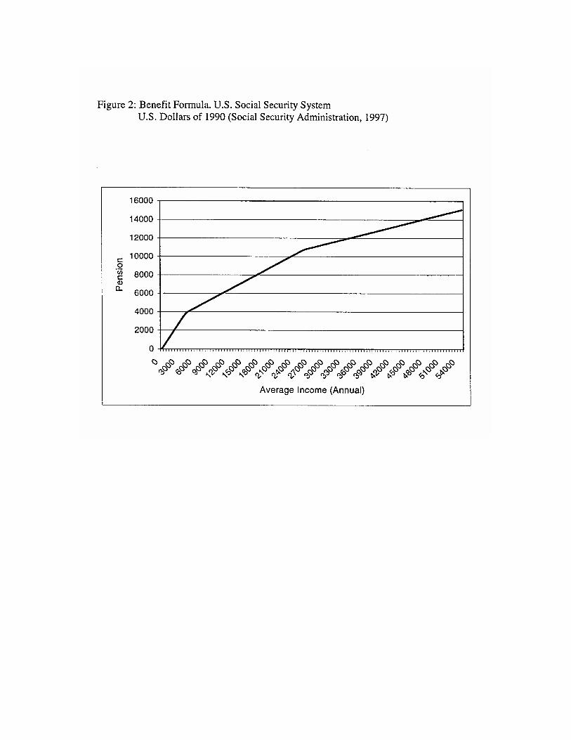
Documentos de TrabajoBanco Central de Chile

Working PapersCentral Bank of Chile

NÚMEROS ANTERIORES PAST ISSUES

La serie de Documentos de Trabajo en versión PDF puede obtenerse gratis en la dirección electrónica:http://www.bcentral.cl/Estudios/DTBC/doctrab.htm. Existe la posibilidad de solicitar una copiaimpresa con un costo de $500 si es dentro de Chile y US$12 si es para fuera de Chile. Las solicitudes sepueden hacer por fax: (56-2) 6702231 o a través de correo electrónico: [email protected]

Working Papers in PDF format can be downloaded free of charge from:http://www.bcentral.cl/Estudios/DTBC/doctrab.htm. Hard copy versions can be ordered individuallyfor US$12 per copy (for orders inside Chile the charge is Ch$500.) Orders can be placed by fax: (56-2)6702231 or email: [email protected]

DTBC-79Evolución del Consumo y Compras de Bienes Durablesen Chile, 1981-1999Francisco Gallego y Raimundo Soto

Septiembre 2000

DTBC-78Monetary Policy in Latin America in The 90sVittorio Corbo

Agosto 2000

DTBC-77Optimal Monetary Policy Rules when The Current Account MattersJuan Pablo Medina y Rodrigo Valdés

Agosto 2000

DTBC-76Value At Risk Ajustado por Liquidez:Una Aplicación a los Bonos Soberanos ChilenosChristian A. Johnson

Julio 2000

DTBC-75Financial Structure in Chile: Macroeconomic Developmentsand Microeconomic EffectsFrancisco Gallego y Norman Loayza

Julio 2000

DTBC-74The Effect of Uncertainty on Monetary Policy:How Good are the Brakes?Adam Cagliarini y Guy Debelle

Junio 2000

DTBC-73Ajuste Estacional e Integración en Variables MacroeconómicasRaimundo Soto

Junio 2000

DTBC-72The Monetary Policy Transmission Mechanism andPolicy Rules in CanadaDavid Longworth y Brian O’Reilly

Mayo 2000

DTBC-71Monetary Policy Rules and Transmission Mechanisms underInflation Targeting in IsraelLeonardo Leiderman and Hadas Bar-Or

Mayo 2000

DTBC-70Optimal Monetary Policy in a Small Open Economy:A General Equilibrium AnalysisCharles Carlstrom y Timothy Fuerst

Abril 2000

DTBC-69Does Inflation Targeting Increase Output Volatility?An International Comparison of Policymakers' Preferencesand OutcomesStephen Cecchetti y Michael Ehrmann

Abril 2000

DTBC-68Chile's Peso: Better Than (Just) Living With the Dollar?Felipe Morandé y Klaus Schmidt-Hebbel

Marzo 2000

DTBC-67Métodos de Evaluación del Riesgo para Portafolios de InversiónChristian Andrew Johnson

Marzo 2000

DTBC-66Policy Biases When The Monetary and Fiscal AuthoritiesHave Different ObjectivesHerman Bennett y Norman Loayza

Marzo 2000

DTBC-65A Note on the Moments of Stochastic Shrinkage Parametersin Ridge RegressionLuis Firinguetti y Hernán Rubio

Marzo 2000

DTBC-64El Encaje, los Flujos de Capitales Y el Gasto:Una Evaluación EmpíricaGuillermo Le Fort y Sergio Lehmann

Febrero 2000

How Does Pension Reform Affect Savings and Welfare

Documents

Transcript of How Does Pension Reform Affect Savings and Welfare