Designing a linear pension scheme with forced savingsand wage heterogeneity1

Helmuth Cremer2, Philippe De Donder3,Dario Maldonado4 and Pierre Pestieau5

March 2006, revised January 2007

1We thank the referees and the editor, Jay Wilson for their detailed comments.2University of Toulouse, GREMAQ and IDEI3University of Toulouse, GREMAQ and IDEI.4Universidad del Rosario, Bogota5University of Liège, CORE, PSE and CEPR.

Abstract

This paper studies the optimal linear pension scheme when society consists of rationaland myopic individuals. Myopic individuals have, ex ante, a strong preference for thepresent even though, ex post, they would regret not to have saved enough. Whilerational and myopic persons share the same ex post intertemporal preferences, only therational agents make their savings decisions according to these preferences. Individualsare also distinguished by their productivity. The social objective is “paternalistic”: theutilitarian welfare function depends on ex post utilities. We examine how the presenceof myopic individuals affects both the size of the pension system and the degree ofredistribution it operates, with and without liquidity constraints. The relationshipbetween proportion of myopic individuals and characteristics of the pension system turnsout to be much more complex than one would have conjectured. Neither the impacton the level of pensions nor the effect on their redistributive degree are unambiguous.Nevertheless, we show that under some plausible assumptions adding myopic individualsincreases the level of pension benefits and leads to a shift from a flat or even targetedscheme to a partially contributory one. However, we also provide an example wherethe degree of redistribution is not a monotonic function of the proportion of myopicindividuals.

Keywords: social security, myopia, dual-self modelJEL classification: H55, D91

1 Introduction

Public pension systems have three main functions. First, they force saving. Some

individuals might be inclined to save less than the amount set aside through payroll

taxes. Second, they redistribute income. Ideally, redistribution should be implemented

by income taxation on a lifetime basis. Unfortunately, such a redistribution is rather

limited in practice and, in most countries, pension systems are viewed as an effective

and politically sustainable way of redistributing income in old age.1 Finally, public

pensions provide insurance in a number of ways pertaining to health, longevity and

financial risks. This paper is concerned with the first two functions, and particularly

the first one.2

Even though the ideas of time inconsistency, myopia and procrastination and the

ensuing need for forced saving have been present in the social security literature for

decades, they have not been that popular in formal work. Redistributive considerations

and concern for dynamic efficiency have dominated most of the theoretical work on social

security. Feldstein (1985) is clearly an exception. His paper examines an overlapping

generation economy with inelastic labor supply in which rational and myopic individuals

coexist.3 It analyses the welfare consequence of introducing a mandatory pension system

and shows that the generosity of this system increases with the proportion of myopic

agents. Feldstein’s model was extended by Imrohoroglu et al. (2000) who introduce

individual income risk, as well as mortality risks and borrowing constraints. They show

that a pay-as-you-go pension system may raise welfare if the time inconsistency problem

is large enough. There is also the recent paper by Diamond and Koszegi (2003) that

is inspired by the hyperbolic discounting literature. Social security is there viewed as a

commitment device.

The last decade has seen the emergence of behavioral economics which explores the

1 In a comparison papier, we look at this issue of political sustainability. See Cremer et al. (2006b)2There is another rationale for public pension that is not considered here and that appears when

there is some sort of welfare or minimum pension. Some middle class workers could be tempted not tosave at all and thus be entitled to such a pension benefit even though they can afford financing theirretirement. By forcing them to save through the pension system, one solves what is known to be the“Samaritan dilemma”. See on this, Pestieau and Possen (2006) and Homburg (2000).

3See also Feldstein (2002), sections 4.1 and 4.2.

1

possible conflict between our preferences for the long-run and our short-run behavior.

The discrepancy between long-run intentions and short-run action is apparent for a wide

range of circumstances and particularly for savings decisions. A number of surveys and

experiments point out that a majority of people believe they should be saving more

for retirement.4 This evidence suggests that households have self-control problems that

call for commitment devices such as a public pension system. Quite interestingly, self-

control problems vindicate the idea of a paternalistic role for the government that for

long was highly controversial.

In general, the self-control problem we have in mind is dealt with in the framework

of hyperbolic preferences. In this paper, we adopt a two-period setting that does not

lend itself to such preferences. Like Feldstein we consider a society in which two types

of individuals coexist: rational ones who don’t have to be forced to save and myopic

ones who, ex ante, have a strong preference for the present even though, ex post, they

would regret not to have saved enough. Like Imrohoroglu et al. (2000), we introduce

explicit liquidity constraints, preventing young individuals from borrowing against their

future pension benefits. Individuals are also distinguished by their productivity. The

government has two objectives: forcing myopic individuals to save enough to support

some basic standard of living throughout retirement and redistributing resources from

high to low earners.

Designing an optimal pension system where all people are rational or myopic is pretty

straightforward. The difficulty comes from mixing the two types and from mixing the

objectives of forced saving and income redistribution.

We adopt a rather simple framework, namely a linear scheme with a payroll tax

with uniform rate and pension benefits that have a contributory (Bismarckian) part

and a flat rate (Beveridgean) part.5 To keep the model simple, we assume that the

4For a survey, see Angeletos et al. (2001).5The nonlinear case is studied in a companion paper (Cremer et al. 2006a). Tenhunen and Tuomala

(2006) also deal with nonlinear lifetime redistribution policies under myopia. Even though the nonlinearapproach is in principle more general, it does not supersede the current paper. Nonlinear models provideinteresting results in terms of marginal tax rates and distortions. However, discrete type models (theonly tractable category in multideminsional taxation models) remain largerly agnostic regarding theproperties of the implementing tax (and pension benefits) functions. Specifically, notions like generorsityand degree of redistribution do not have a clearcut interpretation in that setting. Tenhunen and Tuomala

2

same distribution of productivity prevails in the two groups. The objective of the social

planner is a utilitarian but paternalistic criterion. To be more precise, we consider

the sum of individual utilities in which both rational and myopic individuals are given

the same rate of time preference, namely that of the rational individuals. A main

difference with the papers surveyed above is that the planner optimizes over both the

generosity of pension system (measured by the contribution rate) and the link between

individual pension benefit and past contribution (as measured by a parameter that we

call the Bismarckian factor). Previous papers considered the second characteristic as

exogenously given and concentrated on the contribution rate.

Our main results can be summarized as follows. Let us start with generosity and

concentrate first on “homogeneous” societies (all rational or all myopic, but with indi-

viduals differing in productivity). When all individuals are rational the only justification

of a public pension system is redistribution. The generosity of the system then depends

on the wage inequality and on social preferences for equality. When all individuals are

myopic, the main rationale for a pension system is to secure some level of resources in

the retirement period and the generosity of the system is determined accordingly. Turn-

ing to “mixed” societies, the intuition would suggest that the generosity of the pension

system should increase with the proportion of myopic individuals, in order to make up,

at least in part, for their deficient private savings. This intuition is in line with the

results derived by Feldstein (1985). He shows in a setting with exogenous labor supply

where all workers have the same productivity that generosity unambiguously increases

with the proportion of myopic individuals. In our setting this simple intuition no longer

goes through. We find that increasing the proportion of myopics also has three other

effects, all three pushing towards a less generous system. Consequently, the overall net

impact is ambiguous. These three effects are linked to an increase in labor supply dis-

tortions and to a decrease in the importance of the redistributive motive as myopics get

more numerous–two phenomenons that were not accounted for in Feldstein’s setting.

Turning to the degree of redistribution, we ask if the pension system should be

(2006) measure redistribution by looking at Gini coeficients of first and second period consumption whileCremer et al. (2006a) focus on social welfare.

3

Bismarckian, Beveridgean, or even targeted. With only rational individuals, a pure

Beveridgean system is desirable when there are no binding liquidity constraints. When

the liquidity constraints of some individuals are binding, targeting towards the poor is

desirable (i.e., part of the pension benefits are decreasing with earlier income). With

only myopic individuals, the Beveridgean formula always prevails. When the two types,

rational and myopic households, are combined the pension system typically departs from

the Beveridgean system, but in what direction is not obvious. We argue that targeting

can emerge even in the absence of liquidity constraints (i.e., when the optimal system

for the two groups taken separately is Beveridgean). However, liquidity constraints can

also bring about targeting even when it is not otherwise optimal; this is shown through

numerical examples.

2 The model

Rational individuals’ utility is given by

UR = u(c− v( )) + u(d), (1)

where c and d are first- and second-period consumption, is first-period labor supply,

v( ) is the disutility from working and u(.) is the instantaneous utility from consumption,

net of labor supply disutility. We assume that u0(.) > 0, u00(.) < 0, v0( ) > 0, v00( ) > 0.

In the second period, individuals are retired. This utility (1) is also that of myopic

individuals ex post. Ex ante, myopic agents totally forgo the second period and their

utility is given by

UM = u(c− v( )).

Individuals also differ in productivity w ∈ [w−, w+]. The distribution of w, represented

by the distribution function F (.), is independent of the proportions πR and πM = 1−πRof rational and myopic individuals in the population.6

6 In other words, the distribution of productivities is the same for the two types. This assumptionis made to separate the impact of the proportion of myopics from the impact of the distribution ofproductivity. Other specification could be considered. If, for example, there were a strong positivecorrelation between myopia and productivity we would be in a world of non saving (where peopleare either too poor or too myopic to save) and the generosity of the pension system should be high.

4

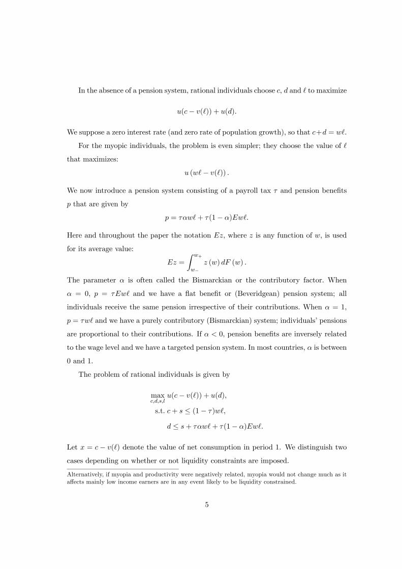
In the absence of a pension system, rational individuals choose c, d and to maximize

u(c− v( )) + u(d).

We suppose a zero interest rate (and zero rate of population growth), so that c+d = w .

For the myopic individuals, the problem is even simpler; they choose the value of

that maximizes:

u (w − v( )) .

We now introduce a pension system consisting of a payroll tax τ and pension benefits

p that are given by

p = ταw + τ(1− α)Ew .

Here and throughout the paper the notation Ez, where z is any function of w, is used

for its average value:

Ez =

Z w+

w−

z (w) dF (w) .

The parameter α is often called the Bismarckian or the contributory factor. When

α = 0, p = τEw and we have a flat benefit or (Beveridgean) pension system; all

individuals receive the same pension irrespective of their contributions. When α = 1,

p = τw and we have a purely contributory (Bismarckian) system; individuals’ pensions

are proportional to their contributions. If α < 0, pension benefits are inversely related

to the wage level and we have a targeted pension system. In most countries, α is between

0 and 1.

The problem of rational individuals is given by

maxc,d,s,l

u(c− v( )) + u(d),

s.t. c+ s ≤ (1− τ)w ,

d ≤ s+ ταw + τ(1− α)Ew .

Let x = c − v( ) denote the value of net consumption in period 1. We distinguish two

cases depending on whether or not liquidity constraints are imposed.

Alternatively, if myopia and productivity were negatively related, myopia would not change much as itaffects mainly low income earners are in any event likely to be liquidity constrained.

5

When there are no liquidity constraints, s can be negative and we have:

u0(xR) = u0(dR),

v0( R) = (1− τ(1− α))w. (2)

Equation (2) yields the labor supply function: R = (w (1− τ (1− α))) . Labor supply

increases with productivity w and with the Bismarckian parameter α, and decreases

with the contribution rate τ .

With liquidity constraints we have s > 0.7 If s > 0, we have the above first-order

conditions. If, however, (1− τ)wlR− v( R) < ταw R+(1−α)Ew , s = 0 and we have:

u0(xR) > u0(dR),

v0(lR) = (1− τ)w +u0(dR)

u0(xR)ταw, (3)

with

xR = (1− τ)w R − v( R),

dR = ταw R + (1− α)τEwl.

Consequently, labor supply depends on w, τ, α for all rational individuals, and also on

Ew for those rational agents who are liquidity constrained.

Turning to the myopic agent, his problem is simply to maximize

u ((1− τ)w − v ( )) ,

which yields

v0 ( M) = (1− τ)w

with

xM = (1− τ)wlM − v(lM),

dM = ταwlM + (1− α)τEwl.

7Assuming liquidity constraints with mandatory (private or public) pensions is both standard andrealistic. It is typically impossible to borrow against the promise of future public pension payments. Evenin the case of private contributive but mandatory schemes, it is generally acknowledged that liquidityconstraints apply (so that contributions to those scheme are distortionary). See on this Summers (1989).

6

We thus obtain M = (w (1− τ)) .

Note that if α = 0, labor supply is identical in each of the three cases, as it depends

only on w (1− τ). This is due to the fact that we have assumed away income effects.

We shall distinguish cases according to whether or not savings can be negative. When

there is no liquidity constraint, savings can be negative. Saving might also be positive

for all rational agents, which is the case when pension benefits are low because, e.g.,

distortions are very high. When savings are strictly positive for all rational agents, we

have u0 (xR) = u0 (dR) . Furthermore, given our assumptions we have u0 (xM) < u0 (dM)

for all myopic individuals. In other words, all myopic individuals, even the poor, consume

more in the first than in the second period. We use this result below.

3 Government’s problem

We now consider the problem of a social planner dealing with a society of rational and

myopic individuals who also differ productivities. Its objective is the sum of ex post

individual utilities, represented by the same utility functions for rational and myopic

individuals. The idea is that ex post the myopic will be grateful to their government for

having forced them to save.

Two words on this specification. First, the use of a utilitarian welfare function is

standard. As an alternative we could have used a Rawlsian criterion which would consist

in maximizing the welfare of the myopic and least productive individuals. Second, we

adopt here an approach that is now called “new paternalism”. According to this view,

paternalistic intervention can be justified to correct problems of self-control.8

Using our compact notation, the problem of the social planner is expressed as follows:

L =X

j=M,R

πj {Eu[w (1− τ) j − sj − v ( j)]

+ Eu [sj + τ (αw j + (1− α)Ew )]} ,8See on this Benabou and Tirole (2002).

7

Differentiating this expression yields:

∂L∂τ

= −X

πj©E£w j

¡u0 (xj)− αu0 (dj)

¢− u0 (dj) (1− α)Ew

¤ª+πMταE

∙w∂ M

∂τu0 (dM)

¸+X

πjEu0 (dj) τ (1− α)Ew

∂ j

∂τ, (4)

∂L∂α

=X

πj

½τ cov

¡w j , u

0 (dj)¢+ (1− α) τEu0 (dj)E

µw∂ j

∂α

¶¾. (5)

Setting these expressions equal to zero yields a system of two equations that jointly

determine the optimal levels of τ and α (as long as the solutions is interior).9 While

generosity and the degree of redistribution are jointly determined it is interesting for

expositional reasons to discuss these issues separately.10 Doing this, we do of course

have to keep in mind that the two variable are not independent.

3.1 Optimal tax rate

We first focus on the optimal tax rate for a given α. Rearranging (4) we obtain,

∂L∂τ

= −X

πj©(1− α) cov[w j , u

0(dj)]−E[w j(u0(dj)− u0(xj))]}

+X

πj(1− α)τE[u0(dj)]E

∙w∂ j

∂τ

¸+ πMταE

∙w∂ M

∂τu0(dM)

¸. (6)

Setting this expression equal to zero and solving yields:

τ =

Pπj [(1− α) cov (w j , u

0 (dj))]−P

πjE [w j (u0 (dj)− u0 (xj))]P

πj (1− α)Eu0 (dj)E³w

∂ j

∂τ

´+ πMαE

³w ∂ M

∂τ u0(dM)´ . (7)

The two terms in the denominator reflect the efficiency concern and depend on the tax

elasticity of labor supply, which is negative. The first term, which relates to the non

contributory part of the pension scheme for all agents, is standard. The second term

focuses on the contributory part for the myopic individuals only, since unlike rational

agents they fail to factor in the link between pensions and contributions when choosing

how much labor to supply. The two terms that compose the numerator reflect the

equity concerns. The covariance term represents the redistributive objective: this term

9Keeping in mind of course that the individual decision variables j and dj are functions of τ and αas discussed in Section 2.10Given the complexity of the problem, a more direct comparative statics approach based on the

sytem (4)—(5) is not very insightful in itself.

8

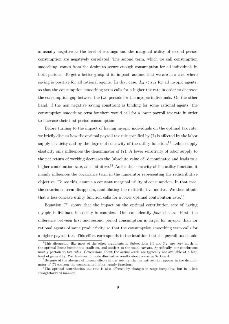
is usually negative as the level of earnings and the marginal utility of second period

consumption are negatively correlated. The second term, which we call consumption

smoothing, comes from the desire to secure enough consumption for all individuals in

both periods. To get a better grasp at its impact, assume that we are in a case where

saving is positive for all rational agents. In that case, dM < xM for all myopic agents,

so that the consumption smoothing term calls for a higher tax rate in order to decrease

the consumption gap between the two periods for the myopic individuals. On the other

hand, if the non negative saving constraint is binding for some rational agents, the

consumption smoothing term for them would call for a lower payroll tax rate in order

to increase their first period consumption.

Before turning to the impact of having myopic individuals on the optimal tax rate,

we briefly discuss how the optimal payroll tax rule specified by (7) is affected by the labor

supply elasticity and by the degree of concavity of the utility function.11 Labor supply

elasticity only influences the denominator of (7). A lower sensitivity of labor supply to

the net return of working decreases the (absolute value of) denominator and leads to a

higher contribution rate, as is intuitive.12 As for the concavity of the utility function, it

mainly influences the covariance term in the numerator representing the redistributive

objective. To see this, assume a constant marginal utility of consumption. In that case,

the covariance term disappears, annihilating the redistributive motive. We then obtain

that a less concave utility function calls for a lower optimal contribution rate.13

Equation (7) shows that the impact on the optimal contribution rate of having

myopic individuals in society is complex. One can identify four effects. First, the

difference between first and second period consumption is larger for myopic than for

rational agents of same productivity, so that the consumption smoothing term calls for

a higher payroll tax. This effect corresponds to the intuition that the payroll tax should

11This discussion, like most of the other arguments in Subsections 3.1 and 3.2, are very much inthe optimal linear income tax tradition, and subject to the usual caveats. Specifically, our conclusionsmostly pertain to tax rules. Conclusions about the actual levels are typically not available at a highlevel of generality. We, however, provide illustrative results about levels in Section 4.12Because of the absence of income effects in our setting, the derivatives that appear in the denomi-

nator of (7) concern the compensated labor supply functions.13The optimal contribution tax rate is also affected by changes in wage inequality, but in a less

straightforward manner.

9

be higher with myopic individuals to compensate for their second period consumption

being too low. However, the other three effects go in the opposite direction. Myopic

individuals save less than rational agents, which tends to reduce the absolute value of

the (negative) average covariance in the numerator of (7); this calls for a lower τ . The

third effect goes in the same direction: with myopic individuals, the contributory part

of the pension scheme generates labor supply distortions, which in turn call for a lower

payroll tax.14 Finally, the marginal utility of second period consumption is larger for

myopic than for rational agents of same productivity, which increases the distortionary

impact of the Beveridgean part of the pension scheme and also calls for a lower payroll

tax. The net effect of the presence of myopic individuals can of course not be assessed by

counting the terms that go one way or the other. The crucial factor is their magnitude

which cannot be assessed at this level of generality. The numerical examples given

below show that the initial intuition may well go through in spite of the presence of

these countervailing effects.

When we compare the extreme settings of πM = 0 (no myopic individuals) and

πM = 1 (all myopic society) the expression is simplified but remains ambiguous. To see

this most clearly we make two additional simplifying assumptions, namely sR > 0 and

α = 0. The assumption that sR > 0 means that no rational individual faces a (binding)

liquidity constraint, which translates in a consumption smoothing term that is nil for

rational agents and positive for myopic individuals. The assumption that α = 0 means

that we concentrate on a Beveridgean system, under which the distortion generated

by the contributory part of the pension system on myopic individuals’ labor supply

disappears.15

The optimal payroll tax with rational agents only is then given by:

τR =− cov (w R, u

0 (dR))

−Eu0 (dR)Eµw∂ R

∂τ

¶ . (8)

14Recall that the contributory part of the pension scheme does not generate distortions for rationalindividuals because they anticipate the induced increase in pensions.15 In the next subsection we will show that in the absence of liquidity constraints α = 0 is effectively

optimal for πM = 0 and πM = 1.

10

With myopic individuals only we have

τM =−E[w M (u

0 (dM)− u0 (xM))]

u0 (dM)E

µw∂ M

∂τ

¶ , (9)

Comparing to the general expression (7), we can notice that the numerator of the

expression for τR does not contain the consumption smoothing term while the nu-

merator of τM has no covariance term (with α = 0, dM is the same for all so that

cov (w M , u0 (dM)) = 0). In spite of these simplifications the comparisons between the

numerators in the expression for τR and τM remains ambiguous. The denominator, on

the other hand can be expected to be larger with myopic individuals. This corresponds

to the fourth effect identified in the discussion of the general expression.

Summing up, the net effect of the presence of myopic individuals on the optimal tax

rate appears to be ambiguous. The numerical examples presented below suggest that

the consumption smoothing term appears to dominate in a wide range of settings. How-

ever, our examples are purely illustrative; the precise comparison remains an empirical

question that requires at the very least simulations based on a calibrated version of the

model.

3.2 The optimal value of the Bismarckian factor

Using ∂ M/∂α = 0, the first-order condition with respect to α, (5), can be rewritten as

∂L∂α

=X

πj©τ cov

¡w j , u

0 (dj)¢ª+ πRτ (1− α) τEu0 (dR)E

µw∂ R

∂α

¶(10)

This condition trades off the anti-redistributive impact of α (which increases consump-

tion inequality, as measured by the first term on the RHS) with its efficiency-enhancing

effect on the labor supply of rational individuals (labor supply of myopics is not affected

by α).16 Here also, the impact of modifying labor supply elasticity and the concavity of

the utility function is clear. Decreasing labor supply elasticity dampens the efficiency-

enhancing effect of linking pension benefits with individual contributions and thus calls

16We can also use (1 − α) as decision variable. Noting that (1 − α)τ represents the net payroll taxrate, (10) can be interpreted as a traditional linear income tax rule.

11

for a lower value of α. Increasing the concavity of the utility function reinforces the

equity concern and also calls for a lower value of α.

To better understand the implications of the proportion of myopic citizens for the de-

termination of the optimal α, we cover successively the cases where society is composed

of myopic agents only, of rational agents only, and of both types of agents.

When society is composed only of myopic individuals, equation (10) simplifies to

∂L∂α

= τ cov¡w M , u0 (dM)

¢,

which is zero when α = 0: with a flat pension dM = p is constant for all w so that

the covariance is equal to zero. Furthermore, when α > 0 the covariance is negative,

while it is positive when α < 0. Consequently, the optimal level of α, denoted by αM

is zero.17 Intuitively, with only myopic agents there is no (efficiency) reason to link

pension benefits to contributions, and the social planner’s redistributive objective leads

to the adoption of a Beveridgean scheme.

We now look at a society composed exclusively of rational agents. Setting (6) equal

to zero and substituting in (10) yields

∂L∂α

=1

1− αEw R

¡u0 (dR)− u0 (xR)

¢+Eu0 (dR)E

∙w

µ∂ R

∂ττ +

∂ R

∂α(1− α)

¶¸. (11)

In the absence of liquidity constraints (or with sR > 0) the first term in (11) vanishes.

Observe that, by equation (2), the labor supply of non liquidity constrained rational

individuals is a function of τ (1− α). It follows that the second term in (11) vanishes

also. Furthermore, only the optimal value of τR¡1− αR

¢matters and thus there is

no single optimal value of αR. To be more precise, the optimal combinations of τR

and αR are defined by the equation τR¡1− αR

¢= τ∗, where τ∗ is the optimal tax

rate conditional on α = 0.18 Intuitively, with non liquidity constrained rational agents,

the payroll tax and the Bismarckian parameter are perfect substitutes. Their optimal

combinations trade off redistribution and the labor supply distortions generated by the

non contributory part of the pension system.17This argument is valid for any level of τ > 0, including the optimal one.18One can also interpret τ∗ as the optimal net payroll tax rate.

12

We now assume that some rational individuals are liquidity constrained. For those

individuals (low-wage earners), dR > xR and

∂ R

∂ττ +

∂ R

∂α(1− α) < 0

by virtue of (3), so that both terms in (11) are negative. Put differently, the perfect

substitutability between τ and α then disappears when some rational agents are liquidity

constrained, and the optimal value of α becomes negative. The intuition for this result

is that introducing targeting into the pension system (by means of a negative value of

α) has nice redistributive properties while being less damaging to efficiency than in the

no liquidity constraint case, since the sensitivity of labor supply to variations of α is

dampened by the lower relative utility of second period consumption.

Finally, when both myopic and rational agents coexist, one can show that

∂L∂α

¯̄̄̄α=0

= πR τ cov¡w R, u

0 (dR)¢+ πRτEu

0 (dR)Ew∂ R

∂α. (12)

The first term of the right hand side is negative but the second one is positive and thus

we cannot sign this expression. Interestingly, this ambiguity arises in the absence of

liquidity constraints. Recall that without liquidity constraints α = 0 is optimal when

society is “homogenous” (only rational or only myopic individuals). However, in a mixed

society, the optimal level of α will in general differ from zero. Specifically, when labor

supply elasticity is small ∂ R/∂α → 0, the second term on the RHS of (12) vanishes

and we obtain a negative level of α. In other words, in the absence of labor market

distortions a very redistributive system is optimal. On the other hand, if the degree of

concavity of u is small (u is close to a linear function), the first term become negligible

and we have α > 0. In that case, redistributive benefits are small and we want to make

the system more Bismarckian to mitigate labor market distortions.

To sum up the main conclusions of this section, we show that τM is likely to be

larger than τR particularly when the rational individuals are not liquidity constrained.

We also show that αR is determined by τR¡1− αR

¢= τ∗ when rational agents are not

liquidity constrained. When they are, αR can be negative. As to αM it is zero. The

sign of the optimal value of α is ambiguous when both rational and myopic individuals

coexist. Table 1 summarizes the results pertaining to the optimal value of α.

13

πR No (binding) liquidity constraints Binding liquidity constraints0 α = 0 α = 0

0 < πR < 1 α S 0 α S 01 τ(1− α) = τ∗ α< 0

Table 1: Summary of Theoretical Results: Optimal Value of α.

In view of such an ambiguity, we now turn to a simulation exercise. This example

not only illustrates our findings but also provides some extra results pertaining to the

actual levels of τ and α that occur in the different case. While these results are not

general, they are instructive in that the show that some patterns of results are effectively

possible.

4 Numerical example

Our numerical simulations are based on the following utility function,

u = log¡c− 2/2

¢+ log d

and a positively skewed Beta(2, 4) distribution for the wages with support (1, 4). Table 2

presents the optimal value of α and τ for alternative values of the proportion of rational

individuals, πR. It also gives the optimal values of τ when α = 0, which we denote by

τ∗. In calculating these values, we assume away any liquidity constraint so that the poor

rational individuals exhibit negative savings. Table 3 presents the same results for the

case where liquidity constraints are imposed.

We start with Table 2. We know from theory that the optimal value of α is zero in

the absence of rational individuals, and that τ and α are perfectly substitutable when

society is composed only of non liquidity constrained individuals. The optimal value of

τ(1−α) when πR = 1 is given by τ∗. The comparison between the optimal Beveridgean

payroll tax when there are only rational individuals who save and when there are only

myopic individuals is in general ambiguous, although we conjectured that it would be

larger with myopic individuals. This conjecture is borne out by the results reported in

Table 2.19

19The situation we simulate in Table 2 is slightly different, since even though all rational agents

14

πR α τ τ∗

0.0000 0.000 0.250 0.2500.1000 0.066 0.247 0.2470.2000 0.122 0.245 0.2430.4000 0.209 0.242 0.2330.6000 0.272 0.239 0.2200.7000 0.298 0.238 0.2110.9000 0.342 0.236 0.2090.9300 0.347 0.236 0.2390.9600 0.353 0.236 0.2200.9900 0.358 0.235 0.2090.9990 0.360 0.235 0.1510.9999 0.360 0.235 0.1511.0000 - - 0.151

Table 2: Optimal linear pension scheme as a function of the proportion of rationalindividuals. No liquidity constraint. We denote τ∗ the optimal tax rate for α = 0.

Recall that the optimal payroll tax rate trades off four concerns, one of them in

favor of a larger tax (consumption smoothing) while three of them plead for a lower tax

(redistributive concern as well as labor supply effects of the non contributory part of

pension for all individuals, and of the contributory part for myopic agents). The presence

of myopic agents tends to increase the consumption smoothing effect. Assuming that the

pension system is Beveridgean (α = 0), it seems reasonable to surmise that the optimal

payroll tax increases with the proportion of myopic agents, which is the result we obtain

in Table 2 by looking at the τ∗ column. Moreover, the optimal value of τ (obtained

by optimizing simultaneously over τ and α) is also increasing with the proportion of

myopic individuals.

The optimum value of α trades off redistribution (calling for moving away from a

Bismarckian system towards a Beveridgean or even a targeted system) and efficiency

(calling for a tighter link between pension benefits and contributions). Since a Bismar-

ckian system fares no better, in efficiency terms, than a Beveridgean one for myopic

equalize marginal utility in both periods, the lowest earners do so by borrowing rather than saving.This means that, although the consumption smoothing term u0(dR)−u0(xR) in (7) is nil for all rationalagents, it is negative for low productivity myopic agents and positive for the other myopic individuals.It is nevertheless reasonable to assume that, on average, the consumption smoothing term is positivefor myopic agents.

15

πR α τ τ∗

0.0000 0.000 0.250 0.2500.1000 0.072 0.246 0.2450.2000 0.131 0.243 0.2400.4000 0.220 0.236 0.2280.6000 0.277 0.230 0.2130.7000 0.295 0.225 0.2030.9000 0.290 0.209 0.1910.9300 0.269 0.202 0.1680.9600 0.232 0.192 0.1600.9900 0.106 0.166 0.1510.9990 -0.184 0.127 0.1480.9999 -0.346 0.111 0.1471.0000 -1.360 0.064 0.147

Table 3: Optimal linear pension scheme as a function of the proportion of rationalindividuals. Liquidity constraint

individuals, intuition suggests that the optimal system would be more and more Bev-

eridgean as the proportion of myopic individuals increases, i.e., that the optimal value

of α should increase with πR. This is what we obtain in Table 2.

We now turn to Table 3. We know from theory that the optimal value of α is zero

in the absence of rational individuals, and is negative when society is composed only of

rational individuals, some of them being liquidity constrained. Comparison of Tables

2 and 3 shows that when all individuals are rational the optimal value of τ(1 − α) is

smaller when a liquidity constraint is imposed on the rational individuals than when

there is no liquidity constraint. This is because when there is a liquidity constraint the

higher tax has a more significant effect on the first period consumption of the poor (who

benefit from the redistribution, but only in the second period). When all individual are

myopic, on the other hand, the liquidity constraint imposed on the rational individuals

is of course irrelevant; this explains why the level of α∗ for πR = 0 is the same in both

tables. We also obtain from Table 3 that the optimal payroll tax when α = 0 is larger

when there are only rational individuals than when there are only myopic individuals.

In other words, the fact that some rational agents are credit constrained and exhibit

a negative consumption smoothing term is not enough to reverse the relationship we

16

πR No (binding) liquidity constraints Binding liquidity constraints0 0 0

0 < πR < 1 > 0 > 0 for low values of πR

< 0 for πR close to 11 τ(1− α) = 0.151 < 0

Table 4: Summary of Numerical Results: Optimal Value of α.

obtain from theory when all rational agents exhibit positive savings. On the other

hand, by comparing the last columns of Tables 2 and 3, it is clear that this consumption

smoothing effect leads to a lower optimal tax rate (conditional on α = 0), when credit

constraints are imposed than when they are not.

We also obtain, in Table 3 as in Table 2, that the optimal payroll tax rate (both

when α is set at zero and when it is also optimized) decreases monotonically with πR.

The main difference between the two Tables lies in the behavior of the optimal α with

respect to the proportion of myopic agents. When some rational individuals are liquidity

constrained, the optimal α first rises then decreases with πR. The largest optimal non

contributory part of the pension system is obtained when 30% of the population consists

of myopic individuals, and decreases as one moves away from that proportion.

Table 4 summarizes our numerical results regarding the optimal value of α.

5 Conclusion

In this paper, we have analyzed the linear pension schemes that ought to be applied

in a society wherein myopic and rational agents coexist and the government forces the

former to save. The foundation of such a paternalistic behavior lies in the fact that

myopic individuals will be grateful in the second period of their life to the government

for having forced them to save for their old age. In other words, myopic agents have two

selves, one looking for immediate gratification and one looking for long term welfare in

the tradition of “dual-self” models (see, e.g., O’Donoghue and Rabin (2001)).

We show that introducing that type of agents in a society of rational individuals has

implications for the level of pension benefits and the redistributiveness of the system

17

that are far more complex than one would have expected. Intuitively one expects that

adding myopic individuals increases the level of pension benefits and leads to a less

redistributive system. We show that this intuition goes through under some conditions.

Specifically, the presence of myopic individuals may even induce a shift from a targeted

scheme to a partially contributory one. However, no definitive results can be obtained

in a general setting and the assessment of net effect appears to be an empirical question.

To keep the analysis simple, we have restricted the pension system to a linear scheme

and we have assumed that the rate of return and the rate of population growth were not

only the same but equal to zero. Relaxing the latter assumption would not change the

qualitative nature of our results. Allowing for a non linear scheme is likely to have strong

implications depending on informational assumptions, as we show in a companion paper

(Cremer et al. (2006a)).

This paper is normative; a paternalistic social planner designs an optimal pension

system, optimal from an ex post standpoint for the myopic individuals. In Cremer et

al. (2006b), we have also analyzed the political economy aspect of the same problem

wherein individuals, myopic and rational, vote ex ante for a pension system. We there

assume that the myopic, when they vote, are in a kind of ”state of grace”, which makes

them choose a commitment device. Interestingly, we obtain results that are parallel to

those found in this paper: the introduction of myopic agents increases the generosity

and decreases the redistributiveness of the pension system.

References

[1] Angeletos, G., D. Laibson, A. Repetto, J. Tobacman and S. Weinberg, (2001), The

hyperbolic consumption model: calibration, simulation and empirical evaluation,

Journal of Economic Perspectives, 15, 47—68.

[2] Benabou, R. and J. Tirole, (2002), Self-confidence and personal motivation, The

Quarterly Journal of Economics, 117:3, 871—915.

[3] Cremer, H., Ph. De Donder, D. Maldonado and P. Pestieau, (2006a), Forced saving,

redistribution and non linear social security scheme, unpublished.

18

[4] Cremer, H., Ph. De Donder, D. Maldonado and P. Pestieau, (2006b), Voting over

type and generosity of a pension system when some individuals are myopic, CORE

DP 2006/79.

[5] Diamond, P. and B. Koszegi, (2003), Quasi-hyperbolic discounting and retirement,

Journal of Public Economics, 87, 1839—1872.

[6] Feldstein, M., (1985), The optimal level of social security benefits, Quarterly Jour-

nal of Economics, 100, 303—321.

[7] Feldstein, M., (2002), Social security, in Handbook of Public Economics, vol. 4, ed.

by A. Auerbach and M. Feldstein, North Holland, Amsterdam, 2246—2324.

[8] Homburg, S., (2000), Compensatory saving in the welfare state, Journal of Public

Economics, 77, 233—239.

[9] Imrohoroglu, A., S. Imrohoroglu and D. Joines, (2003), Time inconsistent prefer-

ences and social security, Quarterly Journal of Economics, 118—2, 745—784.

[10] O’Donoghue, T. and M. Rabin, (2001), Choice and procrastination, Quarterly Jour-

nal of Economics, 116, 121—160.

[11] Pestieau, P. and U. Possen, (2006), Prodigality and myopia. Two rationales for

social security, CORE DP 2006/73.

[12] Summers, L., (1989), Some simple economics of mandated benefits, American Eco-

nomic Review, 79, 177—183.

[13] Tenhunen, S. and M. Tuomala, (2006), On optimal lifetime redistribution policy,

mimeo University of Tampere.

19