1048

HOPE: An Efficie t Parallel Fault Simulator for Svnchronous Seauential Circuits

Hyung Ki Lee and Dong Sam Ha

Abstract- HOPE is an efficient parallel fault simulator for synchronous sequential circuits that employs the parallel version of the single fault propagation technique. HOPE is based on an earlier fault simulator called PROOFS, which employs sev- eral heuristics to efficiently drop faults and to avoid simulation of many inactive faults. In this paper, we propose three new techniques that substantially speed up parallel fault simulation: 1) reduction of faults simulated in parallel through mapping nonstem faults to stem faults, 2) a new fault injection method called functional fault injection, and 3) a combination of a static fault ordering method and a dynamic fault ordering method. Based on our experiments, our fault simulator, HOPE, which incorporates the proposed techniques, is about 1.6 times faster than PROOFS for 16 benchmark circuits.

I. INTRODUCTION

OR THE PAST DECADE, remarkable advances have been made in fault simulation for both combinational and

sequential circuits [ 11-[ 191. Three fault simulation methods, concurrent fault simulation [4]-[7], parallel pattern single fault propagation (PPSFP) [SI-[ 141, and parallel fault simulation combined with single fault propagation [ 11-[3], [ 151-[ 181 are notable due to their efficiency, flexibility, andor versatility.

One of the oldest methods for sequential circuit fault sim- ulation is concurrent fault simulation [4]. In concurrent fault simulation, a fault-free circuit and all the faulty circuits are simulated simultaneously. The biggest advantage of concurrent fault simulation lies in its flexibility and versatility. It can easily accommodate various delay models and functional mod- ules. For this reason, the concurrent fault simulation technique has been widely used for sequential circuits in the industry. Recently, several heuristics that improve the performance of concurrent fault simulation have been proposed [5]-[7]. Even though the speed of concurrent fault simulation has been greatly enhanced, concurrent fault simulation is still slow and requires a large amount of memory.

Single fault propagation has been widely used for combina- tional circuits. In single fault propagation, faults are simulated, one at a time, under the application of a test pattern, and only

Manuscript received September 28, 1993; revised July 8, 1994, February 22, 1995, and June 14, 1995. This work was supported in part by the National Science Foundation under Grant MIP-9310115 and by a SIGDMEEE DATC Design Automation Scholarship Grant. This paper was recommended by Associate Editor W. K. Fuchn.

H. K. Lee was with the Bradley Department of Electrical Engineering, Virginia Polytechnic Institute and State University, Blacksburg, VA 24061 USA. He is now with Cadence Design Systems, Inc., Chelmsford, MA 01824 USA.

D. S. Ha is with the Bradley Department of Electrical Engineering, Virginia Polytechnic Institute and State University, Blacksburg, VA 24061 USA.

Publisher Item Identifier S 0278-0070(96)06722-X.

the differences from the good circuit are simulated. Single fault propagation requires significantly less memory than concurrent fault simulation. For combinational circuits, the performance of the single fault propagation technique has been substan- tially improved by simulating multiple patterns simultaneously [8]. This technique is called PPSFP [8]. Several heuristics have been developed to improve the PPSFP technique for combinational circuits [9]-[ 111. Gouders and Kaibel applied the PPSFP technique to synchronous sequential circuits [ 121. Their PPSFP fault simulator, PARIS, is faster than a parallel fault simulator for most of the ISCAS’89 benchmark circuits [12]. However, for some large circuits, PARIS is substantially slower. Recently, Nair and Ha proposed several heuristics that address the shortcomings of PARIS [13]. Their PPSFP fault simulator, VISION, is, on average, about 1.6 times faster than PARIS for 16 ISCAS’89 circuits, and 3.3 times faster than PARIS for the largest benchmark circuit ~35932. Mojtahedi and Geisselhardt proposed a new fault simulator, COMBINED, which combines the original (single pattern) single fault propagation method and the PPSFP technique used in PARIS [ 141. In COMBINED, faults are initially simulated by applying one pattern at a time. After a certain number of faults are detected, any remaining faults are simulated using the PPSFP technique. Several heuristics were also introduced in [14] to further reduce the fault simulation time.

Cheng and Yu proposed a differential fault simulator (DSIM) for sequential circuits which is based on single fault propagation [ 191. Like single fault propagation, DSIM simulates one fault at a time under the application of a test pattern. The difference is that DSIM simulates each fault, except the first, based on the previous fault simulation result, while single fault propagation processes all faults based on the fault-free circuit simulation. The use of the previous fault simulation result enables DSIM to avoid restoring fault-free values before simulating each fault. Cheng et al. incorporated parallel fault simulation into DSIM [l]. The new fault simulator, PROOFS, simulates a packet of 32 faults in parallel. Niermann et al. added various heuristics to the original version of PROOFS to achieve substantial speedup [2], [3]. By simulating multiple faults in parallel and by utilizing advantages of concurrent fault simulation and single fault propagation, PROOFS speeds up fault simulation compared to DSIM and concurrent fault simulation. In addition, PROOFS reduces memory requirements by about five times. Rudnick et al. proposed a technique which further speeds up PROOFS [15] in the remainder of this paper, PROOFS refers to the version of [2] and [3] enhanced by Niermann et al..

0278-0070/96$05.00 0 1996 IEEE

LEE AND HA: HOPE: AN EFFICIENT PARALLEL FAULT SIMULATOR 1049

In this paper’, we propose three new techniques that sub- stantially reduce the parallel fault simulation time of PROOFS. The new techniques are 1) reduction of faults simulated in parallel through mapping nonstem faults to stem faults, 2) a new fault injection method called functional fault injection, and 3) a combination of a static fault ordering method and a dynamic fault ordering method. We incorporated the proposed techniques into our version of PROOFS to develop a new fault simulator, HOPE. According to our experiments, HOPE is, on average, about 1.6 times faster than our version of PROOFS, and 2.2 times faster than the original PROOFS of [2] for 16 benchmark circuits.

In the next section, we define necessary terms. The tech- niques employed in PROOFS are also reviewed. In Section 111, we present our techniques in detail. In Section IV, experimen- tal results are reported. Section V summarizes the paper.

11. BACKGROUND

In this section, terms necessary to understand the paper are presented. Several heuristics employed in PROOFS are also reviewed. Throughout this paper, single stuck-at faults in synchronous sequential circuits under the zero gate delay model are considered.

A. Terms

A synchronous sequential circuit can be decomposed into flip-flops and a combinational logic block (CLB). The removal of flip-flops turns a sequential circuit into a combinational circuit. The outputs of the flip-flops are called pseudoprimary inputs (PPI’s) and the inputs of the flip-flops are called pseudoprimary outputs (PPO’s). When fanout stems of a combinational circuit are removed, the circuit is partitioned into fanout free regions (FFR’s). Let FFR(t) denote the FFR whose output is t . The output of each FFR can be a stem, a primary output (PO) or a PPO. For the sake of convenience, PO’s and PPO’s are considered as stems in this paper.

An example synchronous sequential circuit is shown in Fig. l(a). Fig. l(b) shows the corresponding CLB after re- moval of flip-flops and the decomposition of the CLB into FFR’s. In a CLB, when all the paths from a line s to PO’s and PPO’s pass through one signal line t , line t is called the dominator of line s [9]. If there is no other dominator between a signal line and its dominator, the dominator is called an immediate dominator. Stem t is a dominator of all lines inside FFR(t). A stem may or may not have a dominator. For example, consider the CLB shown in Fig. l(b). All paths from stem e pass through lines j and 1. Hence, j and 1 are dominators of stem e and j is the immediate dominator. However, stem 1 does not have a dominator.

Under the zero gate delay model, the sequential behavior of a sequential circuit can be simulated by repeating the simulation of the CLB at each time frame. In single fault propagation, all of the faults are simulated, one at a time, under the application of a single test pattern. After simulation of a fault, the faulty values of flip-flops, i.e., PPO’s, which are different from the fault-free values are stored. Since only a

‘Earlier versions of the paper appear in [16] and [17].

PPI

d rn

PPI 1 I

U

d 2-l P I I b 0

C

FFRlll FFR(rn)

FFR(o)

(b)

Fig. 1. An example circuit. (a) A sequential circuit. (b) A partition of the CLB.

portion of flip-flop values (rather than all of the different values of gates in concurrent fault simulation) are stored for each faulty circuit, single fault propagation requires significantly less memory than concurrent fault simulation.

If the effect of a fault f does not propagate to a flip-flop, i.e., a PPO, at a time frame, the fault-free and the faulty values of the corresponding PPI are the same at the following time frame. If the fault-free and the faulty values of all the PPI’s are identical at a time frame, we call the fault a single event fault for the time frame. In this case, it is equivalent to the occurrence of a single fault, and it is necessary to consider only the original fault at the fault site for fault simulation. If there exists at least one PPI whose fault-free and faulty values are different, we call the fault a multiple event fault. A multiple event fault is equivalent to the occurrence of multiple faults for the time frame. Fault simulation must consider the effect of the faulty value(s) of all the PPI(s) whose faulty values are different from fault-free values as well as the original fault. The propagation of the fault effect for a single event fault and for a multiple event fault is illustrated in Fig. 2. The shaded areas in the figure denote the propagation zone of the fault effect. As shown in Fig. 2(a), the fault effect originates only at the fault site for a single event fault. The fault effect originates at multiple sites for a multiple event fault as illustrated in Fig. 2(b). A single event fault at a time frame may become a multiple event fault at another time frame, and vice versa. It is important to note that all faults in a time frame can be grouped into two categories, single event faults and multiple event faults.

Let s/a* denote a stuck-at-a* fault occurred on a line s , where U* E {0, l}. Suppose that the fault s /u * is a single event fault, and suppose that it propagates to a dominator, say t , of the faulty line s. Let the fault-free value and the faulty value of the line t be b and b* , respectively, where b , b* E ( 0 , 1, X } and X denotes an unkndwn state. We can consider a pseudofault which changes the value of the line t from the logic value b to b*. If the faulty value b* is the same

1050 lEEE TRANSACTIONS ON COMPUTER-AIDED DESIGN OF INTEGRATED CIRCUITS AND SYSTEMS, VOL. 15, NO. 9, SEPTEMBER 1996

{ PPI {

{ PPI {

{ PPI {

PO

P PO

1 } PPO

(b)

Fig. 2. Single event fault. (b) Multiple event fault.

Propagation of fault effect for single and multiple event faults. (a)

as the fault-free value b , i.e., the fault s/u* does not propagate to t , we say that the equivalent pseudofault t / b * is insensitive. Otherwise, fault t /b* is sensitive. The following statements hold for pseudofault t /b* .

Statement 1: The pseudofault t /b* is a single event fault. Statement 2: The replacement of the original fault s/u* by

the pseudofault t / b * does not change the behavior of the faulty circuit for the time frame.

The proofs of the above statements are trivial, and are omitted.

The process of replacing the original fault s /u * with a new fault t / b * can be viewed as a mapping of faults. Owing to Statement 2, any single event nonstem fault in FFR(t) can be mapped into a stem fault f t at stem t . The stem fault f t , in turn, can be mapped into another fault at a dominator of the stem (if one exists). This mapping process plays a key role in reducing the number of faults to be simulated in parallel.

Let G ( z ) and F ( z ) be the fault-free value and the faulty value, respectively, at line z under the injection of fault f . Fault f is said to be strongly detected, or simply detected, if G(u) # F ( u ) and G(u) ,F(u ) E { O , l } , at some primary output U . If the fault is not detected and there is a primary output 'U such that G(v) E (0, I} and F ( v ) = X , the fault f is said to be potentially detected. A potentially detected fault may or may not be detected depending on the initial states of flip-flops.

B. PROOFS: A Parallel Differential Fault Simulator PROOFS was introduced first in [ l ] and has been enhanced

in [2] , [3] , and [15]. In PROOFS, the fault-free circuit is simulated first under the application of a test pattern and then a packet of 32 faults are injected and simulated using the bit parallelism inherent in computer words [l]. If a fault is detected, it is dropped from the fault list. After the simulation of a packet of faults, another 32 faults in the fault list are selected and simulated. This process repeats until all faults are simulated for the test pattern. In [2] and [3], several heuristics

have been incorporated into PROOFS to speed up the fault simulation. The three relevant heuristics employed are:

1) reduction of faults to be simulated in parallel; 2) efficient fault injection; 3) efficient fault ordering to reduce the number of gate

evaluations. In the following, we describe the heuristics.

1) Reduction of Faults to Be Simulated in Parallel: If the stuck-at value of a single event fault f is the same as the fault-free value of the faulty line, fault f is not activated. In PROOFS, such faults, called inactive faults, are not in- jected for fault simulation 121. Other active single event faults and all multiple event faults are simulated in parallel. This reduction method was further investigated in 131 and 1151. If a single event fault f is active, the fault simulation attempts to propagate it through one or two gate levels. If the fault fails to propagate beyond one or two gate levels, it is not simulated in parallel. Another method, the so-called star algorithm, is studied in [15]. By incorporating these methods, the performance of PROOFS has been increased by, on average, 17% for the ISCAS'89 benchmark circuits [15].

In this paper, we fully investigate the issue and present a systematic method of reducing the number of faults to be simulated in parallel.

2) Reduction of Fault Injection Time: In the traditional parallel fault simulation method, faults are injected by masking appropriate bits of the words [20], [21]. This method requires chechng every gate during fault simulation to determine whether bit-masking has to be performed and, hence, it is slow. The problem has been circumvented in PROOFS, which modifies the circuit instead of associating bit-masks with gates. A two-input AND or OR gate, depending on the type of the fault, is added to the faulty line [2], [3]. The method avoids checking every gate, but it does incur overhead for circuit modification. Since 32 faults are simulated in parallel, the method requires adding and removing 32 gates for each simulation pass. In addition, the number of events, i.e., the number of gates evaluated, increases due to the added gates.

In this paper, we introduce a new fault injection method that avoids these problems. The new method requires neither circuit modification nor bit-mask checking for every gate.

3) Fault Ordering: In parallel fault simulation, a proper fault grouping is crucial to take advantage of parallelism. Faults that cause the same events should be grouped together into the same packet, if possible. In PROOFS, faults are ordered by a depth first search from outputs toward inputs during preprocessing. During the fault simulation, a group of 32 faults is selected by traversing the ordered fault list from top to bottom. The depth first fault ordering from outputs increases the possibility of grouping faults on the same sensitive path. An experiment shows that depth first fault ordering often reduces the number of events by 50% over a random fault ordering and also shows the best results compared with other variations such as breadth first ordering and ordering from inputs to outputs [3].

The above fault ordering method is static in the sense that the ordering is done only once during preprocessing. In this

LEE AND HA: HOPE AN EFFICIENT PARALLEL FAULT SIMULATOR 1051

paper, we propose new fault ordering methods, a static method and a dynamic method, which further reduce the number of events.

1 stem t

111. PROPOSED METHODS In the previous section, we described the three relevant

heuristics employed in PROOFS. In this section, we present three new techniques which substantially reduce the fault simulation time: 1) reduction of faults to be simulated in parallel through mapping of nonstem faults to stem-faults, 2) a new fault injection method called functional fault injection, and 3) a combination of a static fault ordering method and a dynamic fault ordering method. The three techniques are described below.

Fig. 3. Simulation of nOnStem

FFR(u)

A. Reduction of Faults to be Simulated in Parallel

We propose a new method that reduces the number of faults to be simulated in parallel. As explained in Section 11, faults at a time frame can be categorized into two groups: single event faults and multiple event faults. Our strategy is to reduce the number of single event nonstem faults simulated in parallel in two phases. In the first phase, all single event nonstem faults inside fanout free regions are mapped to the corresponding stem faults by local fault simulation of the nonstem faults. In the second phase, mapped stem faults that are sensitive are examined further for possible elimination from parallel simulation. Throughout the process, a substantial number of faults are screened out before being simulated in parallel. In the following, we explain the process. Faults mentioned in the rest of the section, unless otherwise speciJied, are single event faults. Note that our method does not apply to multiple event faults and all multiple event faults are simulated in parallel in our method.

Phase I-Mapping of Nonstem Faults: Consider a non- stem fault f inside a FFR(t) whose output is stem t . Since stem t is a dominator of the faulty line, the nonstem fault f can be mapped to a stem fault ft using local simulation of the fault. If the mapped stem fault ft is insensitive, the fault is not simulated in parallel. There are three possible mapped stem faults, t / O , t / l , and t / X . Of the three mapped stem faults, the one fault whose faulty value is identical to the fault-free value of the stem is insensitive. Hence, all nonstem faults inside a FFR are essentially mapped to at most two stem faults.

As an example, suppose that there are seven nonstem faults within FFR(t) as shown in Fig. 3. The fault free value of the stem t is 1. Each nonstem fault is mapped into one of the three stem faults, t / l , t / O , or t / X . Since fault t / l is insensitive, all seven of the nonstem faults are reduced to two stem faults, t / O or t / X .

Phase 2-Simulation of Stem Faults: In Phase 1, all non- stem faults are mapped to stem faults. The mapped stem faults are examined further for possible elimination from being simulated in parallel. Consider a mapped stem fault ,ft which has not been eliminated during Phase 1. If stem t is a PO or a PPO, the simulation of f t is trivial. Otherwise, fault ft is examined to determine if it propagates to a certain gate(s) by local fault simulation. If this candidacy test finds that the fault

1

Fig. 4. Simulation of a stem fault with a dominator.

propagates to the gate(s), the fault or another representative stem fault is put into a packet and simulated in parallel. The gate(s) to which the candidacy test attempts to propagate the stem fault depends on whether or not the stem has a dominator, as explained below.

1) Stem Faults with Dominators: If a stem t has a domina- tor, there is a stem U such that FFR(u) includes the immediate dominator of stem t . Note that stem U is unique. The proposed candidacy test examines whether or not the stem fault f t propagates to the following stem U by local fault simulation. In other words, stem fault ft is mapped to another stem fault f u at stem U, and the sensitivity of fu is examined. After mapping fault ft to f u , fault fu is inserted into a packet and simulated in parallel provided that:

1) the line U is a real stem (neither a PO nor a PPO); 2) the fault fu is sensitive; 3) the fault f u has not been simulated in a previous pass

The last condition is attached to ensure that a stem fault is simulated at most once for each test pattern. An example circuit is shown in Fig. 4. Stem t has the immediate dominator v which is included in FFR(u). Stem fault f t at stem t propagates to the following stem U . If Stem fault f u at stem U

has not been already simulated, stem fault fu is injected into a packet and simulated in parallel. After simulation of the fault, the result of the fault simulation is recorded at both stems, t and U . Note that stem fault f u , not the original stem fault f t , is put into a packet for parallel simulation to avoid resimulation of the area FFR(u).

2 ) Stem Faults Without Dominators: If a stem has no dom- inator, the candidacy test is performed on the gates immedi- ately following the stem. If a stem fault f t propagates to any one of the gates, the fault f t is put into a packet and simulated

for the current test pattern.

1052 IEEE TRANSACTIONS ON COMPUTER-AIDED DESIGN OF INTEGRATED CIRCUITS AND SYSTEMS, VOL. 15, NO. 9, SEREMBER 1996

t

Fig. 5. Simulation of a stem fault without dominators

TABLE I GATE TYPE REPRESENTATION

functi; index 1 pmm

B

bit node

faulty line fault type gate type

next

Fig 6 Functional fault injection

yE$- - - inverter

in parallel. Otherwise, the fault2 is dropped from further simulation. An example circuit is shown in Fig. 5. Since stem t does not have a dominator, the immediately following gates U and II are examined. Since fault f t propagates to U , the fault ft is injected in a packet and simulated in parallel.

B. Functional Fault Injection

When a fault is introduced at an input or the output of a gate, the function of the gate changes to reflect the presence of the fault. This suggests that injection of a fault into a circuit can be accomplished by introducing a new type of gate whose function reflects the behavior of the fault. For example, consider a circuit with a two-input exclusive-OR gate whose function is f ( z , y ) = z’y + zy’. Suppose that a stuck-at 1 fault is injected at input y of the exclusive-OR gate. The fault effectively creates a new type of gate whose function is f ( z , y) = 2’. If we replace the original exclusive- OR gate of the circuit with a new type of gate whose function f(z,y) = x’, the stuck-at 1 fault is effectively injected into the circuit. This is the essence of the proposed fault injection method to be described next.

In logic or fault simulation, the types of gates are usually coded in integer numbers and identified by using switch and case statements. Suppose that primitive gate types are coded as shown in Table I. The number assigned to each gate type is called the function index of the gate. Values 1 to 9 are assigned to fault free gates and 20 and above are reserved for faulty gates.

When a fault is injected at an input or the output of a gate, we create a new type of gate. The new type of gate is assigned a function index (20 + the bit position of the fault in the packet). The original function of the new, i.e., faulty, gate, and the description of the fault are stored in a fault descriptor. When multiple faults are associated with a

*It is called one-level inactive fault in [3]

gate, the function index of the new gate is determined as 20 plus the bit position of the first fault to be processed (for implementation purposes). This scheme assigns a unique function index for each faulty gate. Unique function indices for faulty gates offer implementation advantages, but are not required. In the following, we describe the method using an example circuit.

Suppose that three faults, a l l , c / l , and C/O, are injected at gate A, and one fault g/1 at gate B as shown in Fig. 6. Assume that the bit positions in the packet of the four faults, all, c / l , C/O, and g /1 are bit 0 through bit 3. The function indices of the faulty gates and the fault descriptors for the four faults are shown in the figure. (Numbers attached to gates represent function indices.) Assuming that fault a l l , with bit position 0, is processed first, the function index of gate A is set to 20. Since two more faults, c / l and C/O, are to be injected at gate A, the fault descriptors for the two faults are added using a linked list. For gate B, fault g / l at bit position 3 is injected. Hence, the function index of the gate is set to 23. The function index of gate C is 1 as no fault is associated with it. The bit position information in fault descriptors is necessary since multiple faults may be attached to the same gate, as is the case for gate A.

After all faults are injected, the gates are evaluated using the procedure described in Fig. 7. A gate at the lowest level is retrieved from the event queue and the gate function is examined using the switch and case statements. If a gate is fault-free, the gate function is identified through the first nine case statements and evaluated accordingly. (Refer to [2] for gate evaluation details.) Faulty gates are identified by the de- fault statement and evaluated by procedure Faulty-Gate-Eva1 ( ) using the fault descriptors.

Since fault-free gates are examined first inside the switch statement, the above method does not incur any overhead in CPU time for the evaluation of fault-free gates. In addition, as no extra gates are added, it does not add extra events during fault simulation. One shortcoming of the method is that it requires a separate evaluation procedure for the faulty gates which is more complex than that for fault-free gates. Our experimental results, to be presented in the next section, show that the proposed method is better than the circuit modification method of PROOFS for most circuits.

LEE AND HA: HOPE: AN EFFICIENT PARALLEL FAULT SIMULATOR 1053

Procedure EVA( ) (

while (event queue is not empty) I

node = pop (event queue); switch (function index of node) {

case 1: /* AND*/ AND-Eval (node); break;

c a s e 2 /*NAND*/ NAND-Eval (node); break,

case 9 p D type flip-flop */ DFF-Eval (node); break,

Faulty-Gate-Eval (node); break;

default

I

1 1 P End of procedure Eval ( ) */

Fig. 7. Gate evaluation procedure.

Fig. 8. Static fault ordering.

C. New Fault Grouping Methods

As explained in Section 11, PROOFS employs a static fault ordering through a depth first search from outputs during preprocessing. In the following, we propose the combination of two new fault ordering methods, a static fault ordering method performed during preprocessing followed by a dynamic fault ordering method performed during fault simulation.

I ) Static Fault Ordering: Consider the example circuit shown in Fig. 8. Let signal lines a, b, and c be stem lines. Suppose that there are three multiple event faults f l , fi, and f 3 , in FFR(c). Since the effect of the three faults in FFR(c) always passes through to stem c, putting the three faults in the same packet is likely to reduce the number of events. However, when the circuit is traversed by a depth first search, as suggested in PROOFS, faults are ordered as f l , f 2 , FA, f 3 , and FB, where FA and FB represent the ordered fault lists within regions A and B, respectively. If fault lists FA and FB are long, the three faults will not be put in the same packet.

We propose that nonstem faults inside each FFR be grouped first and then the resulting groups of faults be ordered by traversing FFR’s in depth first order from the outputs. The fault ordering is performed once during preprocessing. For the above example, the proposed method arranges faults in the order f l , f 2 , f 3 , FA, and FB. This increases the chance that multiple event nonstem faults inside a FFR are grouped into the same packet. Our experiments show that the proposed fault ordering reduces the number of events by over 6% for the two largest benchmark circuits experimented as compared to the straight depth first fault ordering. It should be noted that the proposed static fault ordering affects only multiple event nonstem faults (which are always put into packets for parallel fault simulation), but not single event nonstem faults which are mapped to stem-faults as described in Section 111-A.

2) Dynamic Fault Ordering: In PROOFS, once the faults are ordered during preprocessing, the order of faults never changes. From our experience, we noticed that the activ- ity of some faults is much higher than other faults dur- ing fault simulation. If high activity faults are grouped to- gether, it is more likely that the propagation paths of the faults overlap with each other, thus reducing the overall gate evaluation time. However, the identification of highly active faults is difficult. The employment of a sophisticated algo- rithm defeats the purpose of reducing the overall processing time.

In fault simulation, the states of all flip-flops are initially set to X . As the simulation progresses, the states of most flip-flops become logic 1 or 0. However, the existence of a fault may prevent some flip-flops from being set to logic 1 or 0, i.e., the flip-flops remain at X . (These faults are called hypertrophic faults [22] .) For a potentially detected fault, there is a flip-flop for which the X value propagates to a PO. This means that the activity of potentially detected faults is high as compared to other faults because the value X propagates all the way from a PPI to the PO. As the X value propagates to a PO, it is likely that the value X also propagates to a PPO. This implies that a potentially detected fault is likely to remain potentially detected in the following time frames. In summary, it is asserted that potentially detected faults are, in general, highly active faults.

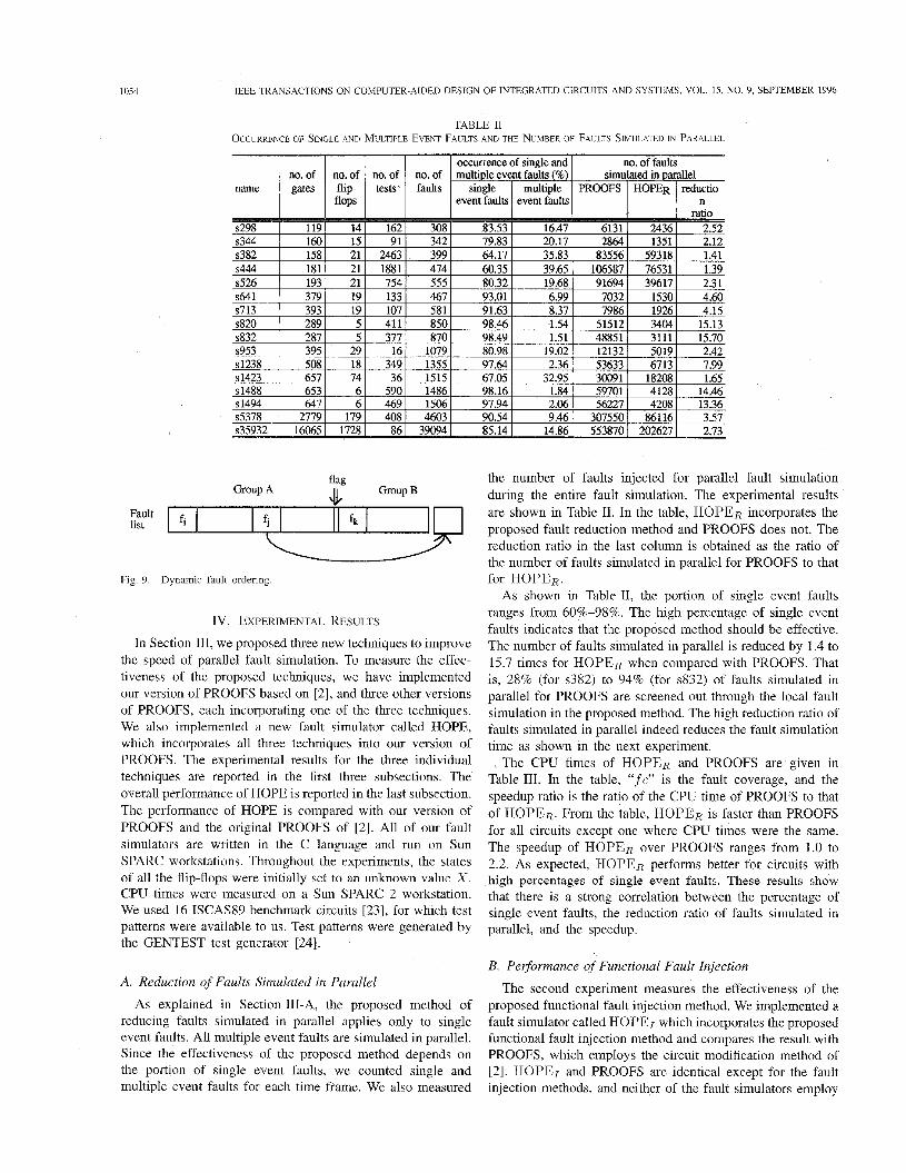
We propose to maintain two groups of faults, group A and group B, in the fault list obtained through the static fault ordering as shown in Fig. 9. Group A contains faults which have not been potentially detected so far, and Group B contains faults which have been potentially detected at least once. Due to the above argument, faults in Group B are likely to be highly active. A fault in group A is moved to Group B whenever it is potentially detected. When faults in the fault list are selected for packets from left to right, faults in Group B are simulated together except for faults at the boundary. The above method moves a fault in group A to group B at most once during the entire fault simulation. Hence, the overhead incurred by the dynamic fault ordering is minimal.

Our experimental results show that the dynamic ordering is effective in reducing the number of events, especially for large circuits. For example, the number of events is reduced by about 20% for the two largest benchmark circuits simulated.

1054 IEEE TRANSACTIONS ON COMPUTER-AIDED DESIGN OF INTEGRATED CIRCUITS AND SYSTEMS, VOL. 15, NO. 9, SEPTEMBER 1996

TABLE I1 OCCURRENCE OF SINGLE AND MULTIPLE EVENT FAULTS AND THE NUMBER OF FAULTS SIMULATED IN PARALLEL

Occurrence of single and no. of faults no. of multiple event faults (%) simulated in parallel faults single multiple PROOFS HOPER reductio

event faults event faults n

flag GroupB k Croup A

list

Fig. 9. Dynamic fault ordering.

IV. EXPERIMENTAL RESULTS

In Section 111, we proposed three new techniques to improve the speed of parallel fault simulation. To measure the effec- tiveness of the proposed techniques, we have implemented our version of PROOFS based on [2] , and three other versions of PROOFS, each incorporating one of the three techniques. We also implemented a new fault simulator called HOPE, which incorporates all three techniques into our version of PROOFS. The experimental results for the three individual techniques are reported in the first three subsections. The overall performance of HOPE is reported in the last subsection. The performance of HOPE is compared with our version of PROOFS and the original PROOFS of [2]. All of our fault simulators are written in the C language and run on Sun SPARC workstations. Throughout thle experiments, the states of all the flip-flops were initially set to an unknown value X CPU times were measured on a Sun SPARC 2 workstation. We used 16 ISCAS89 benchmark circuits [23], for which test patterns were available to us. Test patterns were generated by the GENTEST test generator [24].

A. Reduction of Faults Simulated in Parallel

As explained in Section 111-A, the proposed method of reducing faults simulated in parallel applies only to single event faults. All multiple event faults are simulated in parallel. Since the effectiveness of the proposed method depends on the portion of single event faults, we counted single and multiple event faults for each time frame. We also measured

the number of faults injected for parallel fault simulation during the entire fault simulation. The experimental results are shown in Table 11. In the table, HOPER incorporates the proposed fault reduction method and PROOFS does not. The reduction ratio in the last column is obtained as the ratio of the number of faults simulated in parallel for PROOFS to that for HOPER.

As shown in Table 11, the portion of single event faults ranges from 60%-98%. The high percentage of single event faults indicates that the proposed method should be effective. The number of faults simulated in parallel is reduced by 1.4 to 15.7 times for HOPER when compared with PROOFS. That is, 28% (for s382) to 94% (for s832) of faults simulated in parallel for PROOFS are screened out through the local fault simulation in the proposed method. The high reduction ratio of faults simulated in parallel indeed reduces the fault simulation time as shown in the next experiment.

The CPU times of HOPER and PROOFS are given in Table 111. In the table, “ f e” is the fault coverage, and the speedup ratio is the ratio of the CPU time of PROOFS to that of HOPER. From the table, HOPER is faster than PROOFS for all circuits except one where CPU times were the same. The speedup of HOPER over PROOFS ranges from 1.0 to 2.2. As expected, HOPER performs better for circuits with high percentages of single event faults. These results show that there is a strong correlation between the percentage of single event faults, the reduction ratio of faults simulated in parallel, and the speedup.

B. Performance of Functional Fault Injection

The second experiment measures the effectiveness of the proposed functional fault injection method. We implemented a fault simulator called HOPE1 which incorporates the proposed functional fault injection method and compares the result with PROOFS, which employs the circuit modification method of [2]. HOPE1 and PROOFS are identical except for the fault injection methods, and neither of the fault simulators employ

LEE AND HA: HOPE: AN EFFICIENT PARALLEL FAULT SIMULATOR

name

1055

average no. of average no. of average no. of events faults simulated events per time per time frame per fault per time frame frame

TABLE I11 CPU TIMES WITH AND WITHOUT ELIMINATION OF SINGLE EVENT FAULTS

name fc CPUtime(secs) . speedup

s298 85.71

TABLE IV PERFORMANCE OF THE FUNCTIONAL FAULT INJECTION METHOD

the proposed fault reduction method explained in Section III- A. Experimental results are shown in Table IV. CPU time is the total fault simulation time including the preprocessing time, the good circuit simulation time, and the fault simulation time.

As shown in Table IV, the functional fault injection method performs better than the circuit modification method employed in PROOFS for all circuits except one where the performance is the same. The average speedup is about 1.2. It is notable that the proposed fault injection method achieves the highest speedup, 1.4, for the largest circuit, ~3.5932.

C. Peiformance of Static and Dynamic Fault Ordering

In this section, we report experimental results for the proposed static and dynamic fault ordering methods. The dynamic fault ordering method is based on the hypothesis that faults become more active, i.e., create more events, after they are potentially detected. To verify the hypothesis, we measured the activity of faults before and after their potential detection.

TABLE V ACTIVITY OF FAULTS IN GROUP A AND GROUP B

of events for faults in Group A and faults in Group B represent the activity of faults before and after their potential detection. (Refer to Section 111-C-2 for the description of Group A and Group B). To count the number of events for individual faults, we modified PROOFS to process one fault (instead of a packet of 32 faults) at a time. For each time frame, i.e., under the application of each test pattern, we selected a fault from the list and recorded the group to which the fault belonged. If the selected fault is active, in other words, if the fault-free value of the fault site and the stuck-at value of the fault are different, the fault was injected and the number of events was counted. If the fault is inactive, the fault was not simulated for the time frame. After the fault simulation, the fault was dropped if it was detected, or moved from Group A to Group B if it was potentially detected.

Experimental results are given in Table V. The results for the average number of faults simulated per time frame show that, on average, only 4% of the faults were potentially detected at least once during the fault simulation. However, results for the average number of events per time frame show that those 4% of the faults account for 28% of total events. (The 28% does not include events created by those faults before their potential detection.) The last three columns show that the average number of events caused by a fault per time frame is 9.9 before its potential detection and 159.6 after its potential detection. In other words, the activity of a fault increases by 22 times, on average, after its potential dete~t ion.~ This fact makes the proposed dynamic fault ordering effective, as shown below.

We incorporated static and dynamic fault ordering methods individually and jointly into PROOFS and measured the num- ber of events and CPU time. Experimental results are shown in Table VI and Table VII. In the tables, HOPES is the fault simulator incorporating only static fault ordering, HOPED incorporates only dynamic fault ordering, and H O P E ~ D in- cludes both static and dynamic fault ordering. PROOFS em-

Since a to Group A and then to 3For some circuits, such as s953 and s1238, the activity of faults decreases Group B after it is potentially detected, the average numbers after their potential detection.

1056

s953 s1238 s1423 s1488 s1494

IEEE TRANSACTIONS ON COMPUTER-AIDED DESIGN OF INTEGRATED CIRCUITS AND SYSTEMS, VOL. 15, NO. 9, SEPTEMBER 1996

4296 4521 4274 4513 . 0.95 1.01 0.95 396 398 397 398 0.99 1.00 0.99

3656 3276 3653 3365 1.12 1.00 1.09 1597 1579 1010 1016 . 1.01 1.58 1.57 1856 1858 1123 1131 1.00 1.65 1.64

TABLE VI NUMBER OF EVENTS DURING FAULT SIMULATION

FOR STATIC AND DYNAMIC FAULT ORDERING

name I average no. of events I reduction ratio

s5378 ~35932 average

per pattern PROOFS HOPES HOPED HOPESD HOPES 1 HOPED I HOPESD

s298 196 191 219 s344 257 249 268 264 s382 249 251 232 232 0.99 1.07

5615 5129 4475 4260 . 74643 69911 59869 54748 6018 5685 4902 4566

TABLE VI1 CPU TIMES FOR STATIC AND DYNAMIC FAULT ORDERING

name I CPU time I SDeedUD ratio

ploys depth first ordering from outputs as presented in [2]. It should be noted that none of the implementations given in the table incorporate either the fault reduction method or the new fault injection method.

In Table VI, the number of events is the average number of gates evaluated per test pattern, i.e., per time frame, during fault simulation. Events that occurred during good circuit simulation are not included. The CPU time shown in Table VI1 is the total CPU time, including the preprocessing time, the good circuit simulation time, and the fault simulation time.

Tables VI and VI1 show that both 1.he proposed static fault ordering method and the dynamic fault ordering method are superior to the depth first fault ordering for most circuits with respect to reducing the number of events and CPU time. The average reduction ratio of the number of events is 1.02 for static fault ordering, and 1.17 for dynamic fault ordering. When the static and dynamic fault ordering methods are combined, the number of events is reduced by 1.19. As expected, dynamic fault ordering is more effective than static fault ordering. The speedup ratio for both static and dynamic fault ordering is considerable for large circuits. For the largest

circuit, ~35932, the CPU time is reduced by 5.5 s (from 110.6 s to 105.1 s) for static fault ordering and 11.9 s (from 110.6 s to 98.7 s) for dynamic fault ordering. The above experiments show that i) both the static and dynamic fault ordering methods are effective for large circuits, and ii) the combination of the two methods achieves higher performance than the use of either method alone for most circuits.

Although outside the scope of this paper, the effectiveness of parallei fault simulation versus nonparallel fault simulation can be measured from the above experiments. Table V indicates that the average number of events per test pattern is 13 548 (the sum of the number of events per time frame for Group A and Group B) for nonparallel fault simulation. The average number of events is reduced to 6,018 for parallel fault simulation, as indicated in Table VI. Hence, the parallel fault simulation which simulates 32 faults at a time is about 2.25 times4 more effective than nonparallel fault simulation in terms of the number of events.

D. Overall Pe$ormance of HOPE

The new fault simulator HOPE incorporates all three techniques into our version of PROOFS. The performance of HOPE is compared with our PROOFS and the original PROOFS of [2] in Table VIII. PROOFS0 is the original fault simulator presented in [2] and PROOFS is our version. The CPU times for HOPE and for our version of PROOFS include the preprocessing time including circuit levelization and fault collapsing, the good circuit simulation time, and the fault simulation time. Times for the original PROOFS do not include preprocessing time. All CPU times were measured on a Sun SPARC 2 workstation.

As shown in Table VIII, HOPE achieves better performance than PROOFS0 for all circuits except one, and better perfor- mance than our PROOFS for all circuits. The average speedup of HOPE over PROOFS0 and PROOFS is 2.16 and 1.6, respectively. The speedup is consistent over the wide range of circuits simulated except one. We noticed that all three proposed methods contribute to the improved performance of HOPE. Note that our version of PROOFS is faster than the original PROOFS of [2] for most circuits. Since the CPU time is affected by many factors, including the language, the language compiler, and the code style, the direct comparison of the two fault simulators may be insignificant. (The original PROOFS is written in C++, while our PROOFS is written in C.) Finally, HOPE requires more memory than our PROOFS, but the difference is small. This is mainly attributed to the storage of dominators and fault simulation results for stem faults in HOPE.

In summary, each of the three techniques proposed in Section I11 improves performance as compared to PROOFS for most circuits by reducing the number of faults simulated in parallel, the fault simulation time, and the number of events. The performance of HOPE with respect to circuit size is also worth mentioning. HOPE’S performance depends on several factors, including the portion of single event faults, the number of events per fault and the activity of potentially detected

4This number varies greatly depending on the circuits.

LEE AND HA: HOPE: AN EFFICIENT PARALLEL FAULT SIMULATOR

name

TABLE VI11 PERFORMANCE OF HOPE

CPU time (secs) speedupratio memory

I os7

faults. These factors are all more closely related to the structure of a circuit and the characteristics of test patterns than the size of the circuit. The speedup of HOPE over PROOFS presented in Table VI11 indicates that there is no significant relation between the performance of HOPE in terms of speedup and circuit size.

V. SUMMARY

PROOFS is a highly successful parallel fault simulator for synchronous-sequential circuits [ 11-[3]. PROOFS reduces the CPU time significantly when compared to a concurrent fault simulator, while requiring less memory. The speed of PROOFS is gained by employing the zero gate delay model, the parallel simulation of faults, and utilizing several efficient heuristics.

In this paper, we introduced three new techniques which substantially reduce the fault simulation time. The new tech- niques are: 1) reduction of faults to be simulated in parallel through mapping nonstem faults to stem faults, 2) a new fault injection method called functional fault injection, and 3) a combination of a static fault ordering method and a dynamic fault ordering method. Our experimental results show that each of the proposed techniques is effective in reducing the fault simulation time. The proposed fault reduction method screens out from 28% to 94% of faults which are simulated in parallel in PROOFS. The functional fault injection method achieves an average speedup ratio of 1.2 versus the circuit modification method of PROOFS. On average, the combination of the static fault ordering method and the dynamic fault ordering method reduce the number of events by a factor of 1.19 and enhances the speed by 1.13 times as compared to the depth first fault ordering method employed in PROOFS,

The new fault simulator, HOPE, which incorporates the three new techniques into PROOFS, performs better than our version of PROOFS for all benchmark circuits simulated [ 2 3 ] .

HOPE is about 1.6 times faster than our version of PROOFS and 2.2 times faster than the original PROOFS of [2]. HOPE is expected to be significantly faster than concurrent fault simulators, since PROOFS is much faster than a concurrent fault simulator for the ISCAS’89 benchmark circuits. [ 2 ] .

The speed of HOPE may be improved in at least two ways. Recently, Kung and Lin modified HOPE to process hyper- trophic faults separately [18]. The modified HOPE, called HyHOPE, performs parallel version of serial fault simulation on hypertrophic faults in parallel with fault-free simulation. HyHOPE is about 1.6 times faster than HOPE. Another area which may be worth investigating is reduction of multiple event faults from parallel simulation. We observed that the majority of multiple event faults have a small number of flip-flops, usually one or two, whose faulty values are dif- ferent from fault-free values. Those multiple event faults may be dropped from parallel simulation with proper processing. However, before experimenting with any heuristic, it should be noted that, according to our experience, a sophisticated and, hence, complicated heuristic usually fails to improve the overall speed of HOPE due to the overhead incurred by the heuristic.

ACKNOWLEDGMENT

The authors wish to thank the anonymous reviewers for their constructive suggestions which have improved the presentation of the paper.

REFERENCES

[ I ] W.-T. Cheng and J. H. Patel, “PROOFS: A super fast fault simulator for sequential circuits,” in Proc. Euro. Design Automution Con$, Mar. 1990, pp. 475479.

[2] T. M. Niermann, W.-T. Cheng, and J. H. Patel, “PROOFS: A fast, memory efficient sequential circuit fault simulator,” in Proc. Design Automution Con$, June 1990, pp. 535-540.

1058 IEEE TRANSACTIONS ON COMPUTER-AIDED DESIGN OF INTEGRATED CIRCUITS AND SYSTEMS, VOL. 15, NO. 9, SEPTEMBER 1996

[3] -, “PROOFS: A fast, memory efficient sequential circuit fault simulator,” IEEE Trans. Computer-Aided Design, vol. 11, pp. 198-207, Feb. 1992.

[4] E. G. Ulrich and T. Baker, “The concurrent simulation of nearly identical digital networks,” in Proc. Design Automation Workshop, vol. 6, June 1973, pp. 145-150.

[5] K. Kim and K. K. Saluja, “On fault detection problem in concurrent fault simulation for synchronous sequential circuits,” in Proc. IEEE VLSI Test Symp., Apr. 1992, pp. 125-130.

[6] D. H. Lee and S. M. Reddy, “On efficient fault simulation for syn- chronous sequential circuits,” in Proc. Design Automation CO$, June 1992, pp. 327-331.

[7] D. Saab, “Parallel-concurrent fault simulation,” IEEE Trans. VLSI Syst., vol. I , Sept. 1993, pp. 356-364.

[8] J. A. Waicukauski, E. B. Eichelberger, D. 0. Forlenza, E. Lindbloom, and T. McCarthy, “Fault simulation for structured VLSI,” VLSI Syst. Des., vol. 6, no. 12, pp. 20-32, Dec. 1985.

[9] K. J. Antreich and M. H. Schulz, “Accelerated fault simulation and fault grading in combinational circuits,” IEEE Trans. Computer-Aided I)e.yign, vol. CAD-6, pp. 704-712, Sept. 1987.

1101 F. Maamari and J. Rajski, “A method of fault simulation based on stem regions,” IEEE Trans. Computer-Aided Design, vol. 9, pp. 212-220, Feb. 1990.

[ 1 I ] H. K. Lee and D. S. Ha, “An efficient forward fault simulation algorithm based on the parallel pattern single fault propagation,” in Proc. Int. Test Con$, Oct. 1991, pp. 946-955.

[I21 N. Gouders and R. Kaibel, “PARIS: A parallel pattern fault simulator for synchronous sequential circuits,” in Proc. Int. Conf Computer-Aided Design, Nov. 1991, pp. 542-545.

[I31 R. Nair and D. S. Ha, “VISION: An efficient parallel pattern fault simulator for synchronous sequential circuits,” in Proc. IEEE VLSI Test Symp., Apr. 1995, pp. 221-226.

[14] M. Mojtahedi and W. Geisselhardt, “PARIS: New methods for parallel

1151

1161

U71

sign, Nov. f993, pp. 10-17. 1181 C-P Kung and C-S Lin, “HyHOPE: A fast fault simulator with efficient

pattern fast fault simulation for synchronous sequential circuits,” in Proc. Int. Con$ Computer-Aided Design, Nov. 1993, pp. 2-5. E. M. Rudnick, T. M. Niermann, and J. H. Patel, “Methods for reducing events in sequential circuit fault simulation,” in Proc. Int. Con$ Computer-Aided Design, Nov. 1991, pp. 546-549. H. K. Lee and D. S. Ha, “HOPE: An efficient parallel fault simulator for synchronous sequential circuits,” in Proc. Design Automation Con$, June 1992, pp. 336-340. -, “New methods of improving parallel fault simulation in syn- chronous sequential circuits,” in Proc. Znt. Conf Comauter-Aided De-

~~

simulation of hypertrophic faults,” in P roc. h t . Con$ Computer-Aided Design, Nov. 1994, pp. 714-718.

[19] W.-T. Cheng and M.-L. Yu, “Differential fault simulation-A fast method using minimal memory,” in Proc. Design Automation Con$, June 1989, pp. ,424428.

1201 S. Seshu, “On an improved diagnosis program,” IEEE Trans. Electron. Comput., vol. EC-12, pp. 76-79, Feb. 1965.

1211 E. W. Thomson and S . A. Szygenda, “Digital logic simulation in a time-based, table-driven environment-Part 2. Parallel fault simulation,” Computer, vol. 8, pp. 3 8 4 9 , Mar. 1975.

[22] S. Gai, P. L. Montessoro, and F. Somenzi, “The performance of the concurrent fault simulation algorithms in MOZART,” in P roc. 25th Design Automation Con$, June 1988, pp. 682-697.

[23] F. Brglez, D. Bryan, and K. Kozminski, “Combinational profiles of sequential benchmark circuits,” in Proc. Int. Symp. Circuits Syst., May 1989, pp. 1929-1934.

[24] W.-T. Cheng and T. J. Chakraborty, “Gentest: An automatic test- generation system for sequential circuits,” Computer, vol. 22, pp, 4 3 4 9 , Apr. 1989.

Hyung Ki Lee received the B S degree in elec- tronic engineering from Hanyang University, Seoul, Korea, in 1980, and the M S and Ph D degrees in electrical engineering from Virginia Polytechnic In- stitute and State University in Blacksburg, Virginia, in 1989 and 1994, respectively

After his graduation, he joined the Cadence De- sign Systems Inc., Chelmsford, MA, where he is cuiieiitly working on the development of a test synthesis tool for digital logic circuits. From 1980 to 1986, he was a Research Engineer with the Agency

for Defense Development, Korea. During this period, he was involved in various projects including the development of onhoard equipment for a naval gun and missile control system. His research interests include design automation for digital logic circuits, test synthesis, built-in self testing, fault simulation and automatic test pattern generation.

Dr. Lee is a member of the IEEE Circuits and Systems Society.

Dong Sam Ha was born in Milyang, Korea. He received the B.S. degree in electrical engineering from Seoul National University, Korea, in 1974, and the M.S. and Ph.D. degrees in electrical and computer engineering from the University of Iowa, Iowa City, in 1984 and 1986, respectively.

Since Fall 1986, he has been a faculty member with the Bradley Department of Electrical Engi- neering, Virginia Polytechnic Institute and State University, Blacksburg. Currently, he is an Asso- ciate Professor with the department. He teaches

undergraduate and graduate courses in computer engineering and conducts research in the area of VLSI testing. Prior to graduate study, he served as a Research Engineer with the Agency for Defense Development, Korea. He spent the summer of 1994 with the,German National Research Center for Computer Science (GMD), Bonn, Germany, where he worked on current monitoring testing. Along with his students, he has developed various CAD tools for testing under the support of the National Science Foundation and Design Automation Conference Scholarship grants. He has distributed the source for four tools, two test generators, and two fault simulators including HOPE, to approximately 90 institutions worldwide where these tools are used for teaching and research. His research interests include test generation, fault simulation, built-in self-test, test synthesis, and fault-tolerant system design for automated highway system.