High Quality Wind Data for Energy Systems Models

Iain Staffell, Imperial College London

© Imperial College Business School

High quality wind data for

energy systems models

University of Reading, 5th November 2014

330 GW of capacity

at the start of 2014

33% growth globally

UK has 6th largest

capacity (1st for offshore)

2

Wind power is becoming big

0.1

1

10

100

1995 2000 2005 2010

GW

In

sta

lled

China

US

Germany

Spain

India

UK

330 GW of capacity


33% growth globally

UK has 6th largest


3


330 GW of capacity


33% growth globally

UK has 6th largest


4


330 GW of capacity


33% growth globally

UK has 6th largest


5


6

Motivation

REF study suggested very bad

things for the wind industry.

“normalised load factor for UK onshore

wind farms declines from a peak of

24% at age 1 to

15% at age 10 and

11% at age 15.”

“few wind farms will operate for more

than 12–15 years.”

“The levelised cost for onshore wind

increases from £86/MWh [DECC] to

£183/MWh”

Hughes (2012), p7;

Report Launch Event, De Morgan House, London (19/12/2012)

• The REF study used no weather data

– Argued it was impossible to get hourly wind speeds at 282 sites

• Econometric model chose wind speeds to maximise R²

– The model chose wrong…

7

Motivation

80%

90%

100%

110%

120%

130%

2002 2004 2006 2008 2010

DECC Monthly Wind Index

Hughes Model

Our calculations, based on Hughes’s data.

8

Motivation

• But still people listened…

• Many studies use wind speed data from UK Met masts*

– Sizeable effort required (data cleaning and validation)

– Non-transferable results (where do I get data for Country X?)

– Poor accuracy (correction factors & heuristics needed)

• Reanalysis is an emerging option†

– Data is already cleaned and homogenised

– Global coverage for the last 30 years

– Problem is that ‘data’ comes from a numerical weather

model’s simulation of the atmosphere. Can it be trusted?

9

Simulating wind farm output

*Holttinen, 2005; Sinden, 2007; Strbac et al, 2007; Oswald et al, 2008; Sturt & Strbac, 2011; Green et al, 2014. †Kiss et al, 2009; Pöyry, 2009; Tradewind, 2009; Hawkins et al, 2011; Kubik et al, 2012; Ofgem, 2012.

The Virtual Wind Farm Model

a

(a) Take NASA hourly wind

speeds from MERRA 10

25 m/s

20

15

10

5

0

(b) Interpolate from grid points

to site of each wind farm

The Virtual Wind Farm Model

0%

20%

40%

60%

80%

100%

0 10 20 30

Lo

ad

fa

cto

rWind speed (m/s)

Farm

Turbine

0

20

40

60

80

100

0 2 4 6 8 10 12

He

igh

t a

bo

ve

gro

un

d (

m)

Wind speed (m/s)

NASA data

Log wind profile

Extrapolated speedat hub height

11

(d) Convert from wind speed

to power output using

whole-farm power curve

(c) Extrapolate wind speeds

to hub height with place-

and time-specific parameters

12

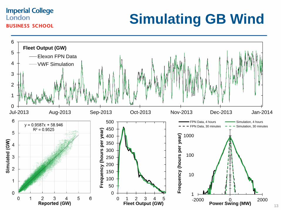
Simulating GB Wind

0

1

2

3

4

5

6

Jan-2012 Jul-2012 Jan-2013 Jul-2013 Jan-2014

Elexon FPN Data

VWF Simulation

Fleet Output (GW)

Staffell, 2014. Developing an Open-Access Wind Profile for Great Britain. Written for DECC.

Results from simulating the GB fleet over two years.

– Comparison made against historic data from the 48 farms

which report their half-hourly output to Elexon

13

Simulating GB Wind

1

10

100

1000

-2000 0 2000

Fre

qu

en

cy (

ho

urs

per

ye

ar)

Power Swing (MW)

FPN Data, 4 hours Simulation, 4 hours

FPN Data, 30 minutes Simulation, 30 minutes

0

50

100

150

200

250

300

350

400

450

500

0 1 2 3 4 5

Fre

qu

en

cy (

ho

urs

per

ye

ar)

Fleet Output (GW)

0

1

2

3

4

5

6

Jul-2013 Aug-2013 Sep-2013 Oct-2013 Nov-2013 Dec-2013 Jan-2014

Elexon FPN Data

VWF Simulation

Fleet Output (GW)

14

Weather Correction

Burradale Wind Farm

15

Weather Correction

0%

10%

20%

30%

40%

50%

60%

70%

80%

2003 2005 2007 2009 2011

Reported monthly load factors Weather corrected load factors

Trend: –0.123 points per year

2013

• Metered output from Burradale

– Can you spot a trend?

• Estimated output if all months had ‘average’ weather

– Reduces the noise and reveals periods of downtime

16

Weather Correction

0%

10%

20%

30%

40%

50%

60%

70%

80%

2003 2005 2007 2009 2011



2013

• Find the average rate of decline

– Fit a straight line (as we economists are simple people)

17

Weather Correction

0%

10%

20%

30%

40%

50%

60%

70%

80%

2003 2005 2007 2009 2011



2013

• Repeat for all 282 large

farms in the UK

• Average farm loses

0.4 ± 0.1 points per

year

– Decline from 28.5%

new to 21% at age

19

• Degradation adds 9%

to the levelised cost of

wind

18

How do wind farms degrade?

0

5

10

15

20

25

30

-3 -2 -1 0 1 2 3

Nu

mb

er

of

farm

s

Degradation rate (annual change in CF)

Late 2000s

Early 2000s

Late 1990s

Early 1990s

Cauchy fit

• Are more recent

turbines performing

better?

• Large spread of

results – need to

increase n to

decrease σ

• What are the

engineering causes?

• So… more work to do…

19

How do wind farms degrade?

Mo

re r

ece

nt

Faster decline

• Mechanical wear?

• Early death?

• Increasing downtime?

• O&M practices?

20

Why do wind farms degrade?

• MSc project to validate

MERRA in other countries

– 5,000 individual turbines

in Denmark

– 350 farms in the US

• Try to match monthly

output from 2001 to

2014

21

Expanding the Study

X. Yao, 2014. Assessing the reliability of NASA MERRA in estimating wind power outputs.

• Similar quality of

results to the UK

– 60% of turbines

have a monthly R²

over 90%

– Overall average is

only 82%, which

can improve with

data cleaning

• To be expected?

– DK is rather similar

to UK after all…

Validation in Denmark

22 X. Yao, 2014. Assessing the reliability of NASA MERRA in estimating wind power outputs.

• Very mixed results

– R² averages 49%

– 64% in central and

eastern US

– Just 13% on the

west coast –

completely wrong

seasonal pattern!

23

Validation in the US

X. Yao, 2014. Assessing the reliability of NASA MERRA in estimating wind power outputs.

• Poorest performance all grouped on the west coast

24


• Poorest performance all grouped on the west coast

• MERRA’s spatial resolution is an obvious flaw

• But how does this translate to seasonal trends?

25


MERRA: 3TIER:

26

And now for something

completely different…

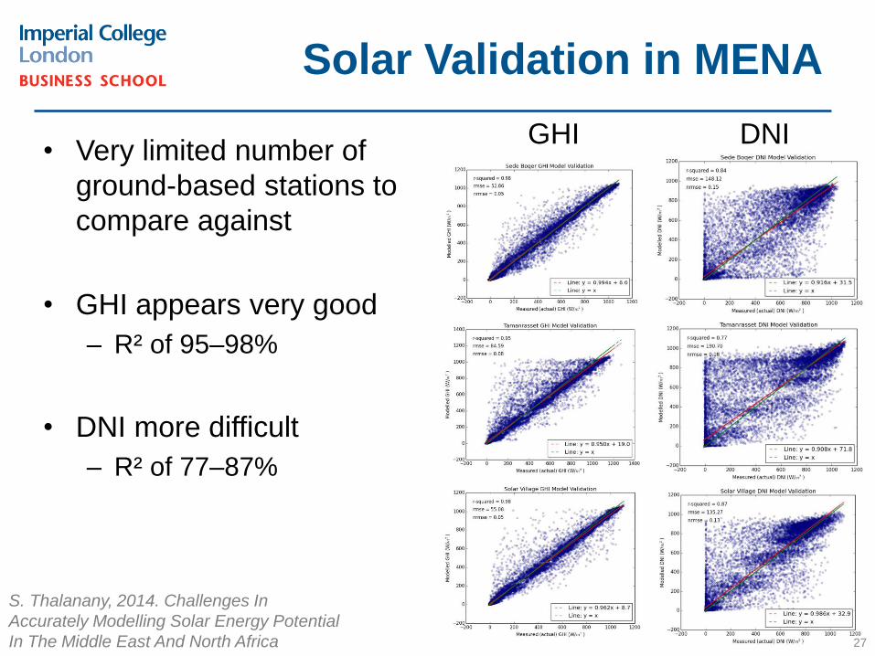
• Very limited number of

ground-based stations to

compare against

• GHI appears very good

– R² of 95–98%

• DNI more difficult

– R² of 77–87%

Solar Validation in MENA

27

DNI GHI

S. Thalanany, 2014. Challenges In

Accurately Modelling Solar Energy Potential

In The Middle East And North Africa

• Modelling PV panels is relatively good

• 227 panels, 17 locations, summary of individual R²

• Quality more dependent on meta-data than solar data

28

Solar Validation in the UK

S. Thalanany, 2014. Challenges In Accurately Modelling Solar

Energy Potential In The Middle East And North Africa

• Failure to represent the wind properly can yield very

wrong results

• The Virtual Wind Farm model can robustly simulate the

half-hourly outputs from UK wind farms

• It has demonstrated how output declines gradually with

age

– This rate is similar to other turbine machinery

– Lost energy adds 9% to the levelised cost of electricity

• There is a lot more to learn about degradation…

• There are many other energy systems modelling tasks

that this could be used for… 29

Conclusions

http://tinyurl.com/wind-decline [email protected]

30

Conclusions

http://tinyurl.com/wind-decline



mailto:[email protected]

32

Backup slides

• Current UK fleet (~10 GW)

33

Evolving National Output

0

20

40

60

80

20-Dec 27-Dec

GW Current + Planned + Offshore

• Approved and under construction (~20 GW)

34


0

20

40

60

80

20-Dec 27-Dec


• Round 2 and 3 ‘super offshore’ (~50 GW)

35


0

20

40

60

80

20-Dec 27-Dec


37

Diversity in Europe

0%

10%

20%

30%

40%

50%

60%

70%

80%

90%

100%

01-Jan 05-Jan 09-Jan 13-Jan

UK

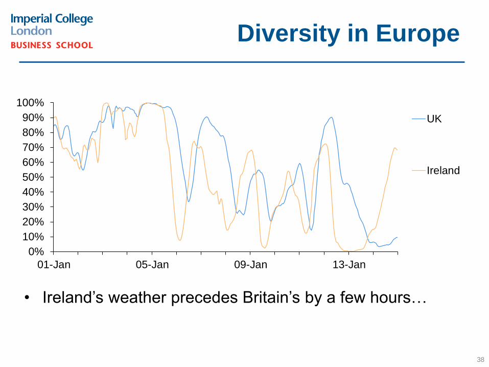
• Ireland’s weather precedes Britain’s by a few hours…

38

Diversity in Europe

0%

10%

20%

30%

40%

50%

60%

70%

80%

90%

100%


UK

Ireland

• Small smoothing effect by combining their outputs…

39

Diversity in Europe

0%

10%

20%

30%

40%

50%

60%

70%

80%

90%

100%


UK

Ireland

Combined

• France is at lower latitudes and gets different weather…

40

Diversity in Europe

0%

10%

20%

30%

40%

50%

60%

70%

80%

90%

100%


UK

Ireland

France

Combined

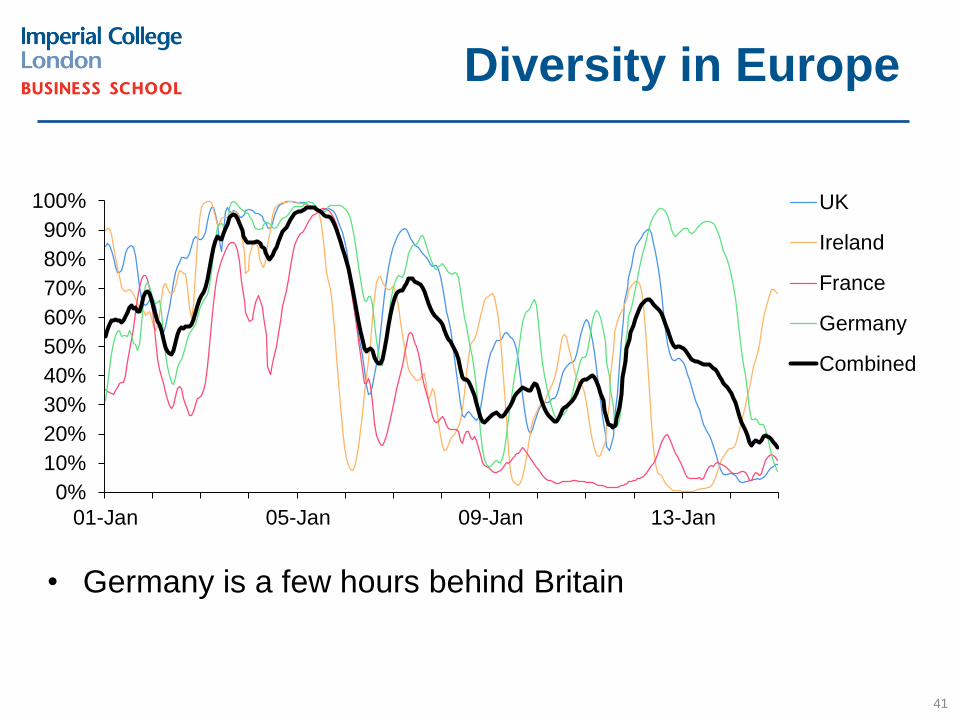
• Germany is a few hours behind Britain

41

Diversity in Europe

0%

10%

20%

30%

40%

50%

60%

70%

80%

90%

100%


UK

Ireland

France

Germany

Combined

• The variance across 5 neighbours is reduced by a third…

– Based on assumed 2020 installed capacities

42

Diversity in Europe

0%

10%

20%

30%

40%

50%

60%

70%

80%

90%

100%


UK

Ireland

France

Germany

Norway

Combined

• Tweak the ratio of capacities (lots more in Norway) and

variance is less than half…

– At the expense of some output…

43

Diversity in Europe

0%

10%

20%

30%

40%

50%

60%

70%

80%

90%

100%


UK

Ireland

France

Germany

Norway

Combined

High Quality Wind Data for Energy Systems Models

Documents

Transcript of High Quality Wind Data for Energy Systems Models