High Noon for Microfinance Impact Evaluations: Re-investigating the Evidence from Bangladesh
41
High Noon for Microfinance Impact Evaluations: Re-investigating the Evidence from Bangladesh Maren Duvendack and Richard Palmer-Jones The School of International Development, University of East Anglia Norwich, NR4 7TJ, United Kingdom 2011 Working Paper 27 Working Paper Series ISSN 1756-7904
-
Upload
eastanglia -
Category
Documents
-
view
1 -
download
0
Transcript of High Noon for Microfinance Impact Evaluations: Re-investigating the Evidence from Bangladesh

Electronic copy available at: http://ssrn.com/abstract=1735615
High Noon for Microfinance Impact Evaluations: Re-investigating the Evidence from Bangladesh
Maren Duvendack and Richard Palmer-Jones
The School of International Development, University of East Anglia Norwich, NR4 7TJ, United Kingdom
2011
Working Paper 27
Working Paper Series
ISSN 1756-7904

Electronic copy available at: http://ssrn.com/abstract=1735615
2
DEV Working Paper 27
High Noon for Microfinance Impact Evaluations: Re-investigating the Evidence from Bangladesh Maren Duvendack and Richard Palmer-Jones First published by the School of International Development in January 2011. This publication may be reproduced by any method without fee for teaching or nonprofit purposes, but not for resale. This paper and others in the DEV Working Paper series should be cited with due acknowledgment. This publication may be cited as: Duvendack, M. and Palmer-Jones, R., 2011, High Noon for Microfinance Impact Evaluations: Re-investigating the Evidence from Bangladesh, Working Paper 27, DEV Working Paper Series, The School of International Development, University of East Anglia, UK. About the Authors Maren Duvendack is a Senior Research Associate in the School of International Development at the University of East Anglia, Norwich, UK. Richard Palmer-Jones is a Reader in Economics at the School of International Development at the University of East Anglia, Norwich, UK. Contact: Email: [email protected] School of International Development University of East Anglia Norwich, NR4 7TJ United Kingdom Tel: +44(0)1603 592329 Fax: +44(0)1603 451999 ISSN 1756-7904

3
About the DEV Working Paper Series The Working Paper Series profiles research and policy work conducted by the School of International Development and International Development UEA (see below). Launched in 2007, it provides an opportunity for staff, associated researchers and fellows to disseminate original research and policy advice on a wide range of subjects. All papers are peer reviewed within the School. About the School of International Development The School of International Development (DEV) applies economic, social and natural science disciplines to the study of international development, with special emphasis on social and environmental change and poverty alleviation. DEV has a strong commitment to an interdisciplinary research and teaching approach to Development Studies and the study of poverty. International Development UEA (formerly Overseas Development Group) Founded in 1967, International Development UEA is a charitable company wholly owned by the University of East Anglia, which handles the consultancy, research, and training undertaken by the faculty members in DEV and approximately 200 external consultants. Since its foundation it has provided training for professionals from more than 70 countries and completed over 1,000 consultancy and research assignments. International Development UEA provides DEV staff with opportunities to participate in on-going development work, practical and policy related engagement which add a unique and valuable element to the School's teaching programmes. For further information on DEV and the International Development UEA, please contact: School of International Development University of East Anglia, Norwich NR4 7TJ, United Kingdom Tel: +44 (0)1603 592329 Fax: +44 (0)1603 451999 Email: [email protected] Webpage: www.uea.ac.uk/dev

Duvendack, M. & Palmer-Jones, R. DEV Working Paper 27
4
Acknowledgements We wish to thank David Roodman for supporting the data set re-construction and Matthieu Chemin for sharing some Stata do-files to allow us to comprehend his data analysis. Many thanks also to the World Bank for providing additional data files that were not available online but essential for our analysis. Thanks very much to Ben D’Exelle for a critical review.

Duvendack, M. & Palmer-Jones, R. DEV Working Paper 27
5
Abstract Recently, microfinance has come under increasing criticism raising questions of the validity of iconic studies which have justified the microfinance phenomenon. This paper applies propensity score matching (PSM), which has become widely used for the analysis of observational data, to the study by Pitt and Khandker (1998) which has been labelled the most rigorous evidence supporting claims that microfinance benefits the poorest especially when targeted on women. After carefully reconstructing the data we differentiate outcomes by gender of borrower, take account of borrowing from several formal and informal sources, and find that the mainly positive impacts of microfinance that we observe are shown by sensitivity analysis to be highly vulnerable to selection on unobservables, and we are therefore not convinced that the relationships between microfinance and outcomes are causal. Introduction The concept of microcredit was first introduced in Bangladesh by Nobel Peace Prize winner Muhammad Yunus. Professor Yunus started Grameen Bank more than 30 years ago aiming to reduce poverty by providing small loans to the countries’ rural poor (Yunus, 1999). It is argued that microfinance can not only enable the poor to access credit, providing them access to remunerative activities and relieving them of onerous debts (Khandker, 1998; 2000). A key feature of the Grameen Bank and many other microfinance organisations has been the targeting of women on the grounds that, compared to men, they perform better as microfinance institution (MFIs) clients and that their participation has more desirable development outcomes, an argument that is most authoritatively supported by Pitt and Khandker (1998 – henceforth PnK). However, despite the apparent success and popularity of microfinance, it is widely argued that there is little convincing evidence yet that microfinance programmes have positive impacts (Armendáriz de Aghion and Morduch, 2005; 2010); for reviews of microfinance impact evaluations reiterating this point see also Sebstad and Chen, 1996; Gaile and Foster, 1996; Goldberg, 2005; Odell, 2010). A number of putatively rigorous studies suggest social and economic benefits from microfinance (Hulme and Mosley, 1996; PnK; Khandker, 1998, 2005; Coleman, 1999; Rutherford, 2001; Morduch and Haley, 2002). However, Dichter and Harper (2007), Roodman and Morduch (2009 – henceforth RnM) and Bateman and Chang (2009) argue that microfinance is neither always beneficial nor rigorously demonstrated. The debate over microfinance impact intensified recently with the publication of the first two randomised control trials (RCTs) in the sector (Banerjee et al, 2009; Karlan and Zinman, 2009) which both raise doubts about the causal link between microfinance participation and poverty alleviation. Many of the early microfinance impact evaluations fail to address the problem of selection bias (Sebstad and Chen, 1996; Gaile and Foster, 1996); selection bias occurs

Duvendack, M. & Palmer-Jones, R. DEV Working Paper 27
6
because participants self-select or are selected into a programme (in a non-random way), and therefore differ from those who are not selected; this undermines simple impact estimates based on non-random control groups (Heckman, 1979). A few studies of microfinance have addressed this problem more thoroughly (for example Hulme and Mosley, 1996; PnK); these studies, however, have not been uncontested1
.
This paper re-examines the evidence of what is commonly seen as the most authoritative microfinance impact evaluation (RnM) which was conducted by PnK on three microfinance programmes in Bangladesh. The challenges of microfinance impact evaluations which PnK (Morduch, 1998; RnM) address is to account for participant selection and program placement2 biases (PnK; Coleman, 1999); PnK do this using a specific model (see below), and Khandker (2005 – henceforth Khandker) adds data on the same households to construct a panel, putatively overcoming at least the problems for evaluation posed by participant selection. A number of studies have attempted to replicate the findings of the original PnK study, and of Khandker. For example, Morduch (1998 – henceforth Morduch) contested PnK but was seemingly refuted by Pitt (1999 – henceforth Pitt)3
. RnM with considerable effort and difficulty replicated PnK and Khandker, producing variables which in some cases differ significantly from their equivalent in PnK and Khandker, and, using different estimating software, find no convincing evidence for either impact claimed by PnK and Khandker.
Chemin (2008 – henceforth Chemin), applies propensity score matching (PSM) to his construction of the PnK data; PSM has become a very popular technique in the area of development economics in recent years; it has roots in the literature on experiments beginning with Neyman (1923). Rubin (1973a, b; 1974; 1977; 1978) expands on this literature and laid the conceptual foundations of matching. The technique has been further refined in particular by Rosenbaum and Rubin (1983; 1984). PSM is performed by matching participants to non-participants drawn from a suitable population using a predicted probability of programme participation or the ‘propensity score’ (Ravallion, 2001; Caliendo and Kopeinig, 2005; 2008). The treatment effect is then estimated by comparing the mean outcomes of the participants and their matches (Ravallion, 2001). This method can account for selection bias due to observable characteristics used in the matching process. Its drawback, however, is that bias due to selection on unobservables remains (Smith and Todd, 2005). Selection on unobservables, or ‘hidden bias’ as Rosenbaum (2002) calls it, are driven by unobserved variables that influence treatment allocation as well
1 Hulme and Mosley (1996) were contested by Morduch (1999) and PnK by Morduch (1998) and RnM. 2 The locations of programmes are also chosen in a non-random way and therefore differ from other places that could be used as controls. 3 The complexity of the PnK and Pitt method, using unique and unrecoverable computer code (see footnote 21 for correspondence between Roodman and Pitt), seemingly meant this debate remained unresolved in the grey literature until RnM replicated PnK.

Duvendack, M. & Palmer-Jones, R. DEV Working Paper 27
7
as potential outcomes (Becker and Caliendo, 2007). Sensitivity analysis of PSM results can identify the vulnerability of the estimated impact to unobservables (Rosenbaum, 2002). With his construction of the relevant variables from the unit level PnK data, Chemin finds statistically significant but smaller effects than those of PnK on all outcome variables except male labour supply (Chemin: 478). However, he does not distinguish outcomes by the gender of borrowers and does not apply sensitivity analysis, which is good practice in PSM studies (Ichino, Mealli and Nannicini, 2006; Nannicini, 2007). In this paper we apply PSM to our construction of the relevant variables, examine the effects of the gender of the borrower, and subject the results to sensitivity analysis; first we reconstruct the data. We find differences from variables reported in Chemin (but only minor differences from RnM4), and draw attention to borrowing from sources other than microfinance by sample households. Borrowing from MFIs may substitute (Khandker, 2000), or complement (Fernando, 1997; Coleman, 1999) borrowing from other sources. Borrowing from more than one source may occur either because the borrower requires more finance than a single MFI will supply5
, or because further finance is needed to make repayments (Fernando, 1997; Coleman, 1999; Venkata and Yamini, 2010). We apply sensitivity analysis to assess the robustness of our results and reflect on the usefulness of PSM in the context of these data.
The paper proceeds as follows: we briefly discuss the challenges of replication and (re-) construction of appropriate variables with the PnK data, and briefly introduce PSM and sensitivity analysis. We then outline the particularities in PnK’s research design, apply PSM to (our reconstruction of) the PnK data, investigate effects of the gender of the borrower and the role of borrowing from other sources (by microfinance members and others) on microfinance impact; we apply sensitivity analysis to the matching results to draw conclusions as to the robustness and limitations of PSM in this context and what seems reasonable to conclude with regard to the impacts of microfinance by applying PSM to these data. While our PSM results suggest that microfinance participation has some significant impacts (negative as well as positive), they are in general not distinguishable from those of other sources of finance. Moreover, sensitivity analysis shows that all impacts are very sensitive to unobservables, which are therefore quite likely to have confounded the results. We conclude that, properly applied with sensitivity analysis, PSM resolves the particular problems in the PnK study by showing that it cannot
4 Because our constructed variables are so similar to those of RnM we do not exhaustively compare our variables to either RnM or PnK; we note differences with RnM in the relevant places. 5 Including cases where microfinance borrowers may not be able to borrow sufficient to repay all previous outstanding loans from other sources (Coleman, 1999).

Duvendack, M. & Palmer-Jones, R. DEV Working Paper 27
8
generate robust conclusions of impact with these outcome variables6
. However, PSM may not be an appropriate tool because the data set does not contain a suitable, large and relatively homogeneous control group. Hence, by extension, PSM may not be the miracle tool implied by the recent epidemic of applications, as we discuss below.
Replication challenges The objective of replication is to allow other researchers to assess the robustness of the findings (Hamermesh, 2007), and is a characteristic of natural if not social science. To allow replication, good documentation of the study design and data are required, and there should be access to the data, and details of their variable construction and analysis7
.
In the case of PnK, most of the data, including questionnaires and variable codes are (at the time of writing this paper) available on the World Bank website8 but replication remains a challenge. Firstly, the survey forms and variable descriptions are problematic; secondly certain data necessary for replication were (and others are) missing9. Some of these data10 were obtained after contacting the authors (either by Roodman, or ourselves). The replication exercise reported here was greatly facilitated by RnM who have made all their data and codes available11
.
We have compared our data with RnM’s data, variable by variable; remaining minor discrepancies reflect differences in our interpretation of some variables. Nonetheless, re-running RnM’s Stata do-files using our data set very closely approximates their substantive results. RnM replicated the key PnK studies12
6 Other outcome variables have been addressed in other papers using the PnK dataset (Pitt et al, 1999; Pitt, 2000; McKernan, 2002; Pitt and Khandker, 2002; Pitt et al, 2003; Pitt, Khandker and Cartwright, 2006).
, using similar estimation
7 The American Economic Review (AER), for example, requires its authors to make their data sets and code available which are then uploaded onto a website maintained by the AER especially for this purpose. Authors have been compliant with this policy so far but can opt out in case their data are proprietary and/or confidential (Hamermesh, 2007: 717). 8http://econ.worldbank.org/WBSITE/EXTERNAL/EXTDEC/EXTRESEARCH/0,,contentMDK:21470820~pagePK:64214825~piPK:64214943~theSitePK:469382,00.html. All data used for this paper come from this source. 9 It is not possible to be sure that the data posted are indeed exactly the same as those analysed by PnK, but the main problems probably lie not in variations in the raw data but in subsequent manipulations, variable constructions, and analytical procedures. 10 Such as data on consumer price indices, sampling weights and landholding details. 11 http://www.cgdev.org/content/publications/detail/1422302. The data and variable construction are mainly in SQL, although statistical analysis is in Stata; our data manipulation and analysis is all in Stata. 12 RnM do not replicate Chemin or a few other studies that used the PnK data (Khandker, 1996, 2000; Pitt et al, 1999; Pitt, 2000; McKernan, 2002; Pitt and Khandker, 2002; Pitt et al, 2003; Menon, 2006; Pitt, Khandker and Cartwright, 2006).

Duvendack, M. & Palmer-Jones, R. DEV Working Paper 27
9
strategies but different software13
. They find that ‘decisive statistical evidence in favor of [the idea that microcredit alleviates poverty, smoothes household expenditure and lessens the pinch of hunger especially when women are involved in borrowing] is absent from these studies’ (RnM: 40). We apply PSM which, as used by Chemin, currently provides the only remaining credible evaluation of microfinance using these data.
The Impact of Microfinance in Bangladesh PnK use data from a World Bank funded study which conducted a survey in three waves in 1991-199214
on three leading microfinance group-lending programmes in Bangladesh, namely Grameen Bank (GB), the Bangladesh Rural Advancement Committee (BRAC) and the Bangladesh Rural Development Board (BRDB) (PnK: 959). A quasi-experimental design was used which sampled target (having a choice to participate/being eligible) and non-target households (having no choice to participate/not being eligible) from villages with microfinance programme (treatment villages) and non-programme villages (control villages).
The survey was conducted in 87 villages from 29 thanas15; the treatment villages were randomly selected from a list of villages provided by the MFIs’ local offices and the control villages were randomly selected from the governments’ village census; 1,798 households were selected out of which 1,538 were target households and 260 were non-target households (PnK: 974). According to PnK (974), out of those 1,538 households, 905 effectively participated in microfinance (59%). The three survey waves (henceforth R1-3) were timed to account for seasonal variations, (Pitt, 2000:28-29). The study focuses on measuring the impact of microfinance participation by gender on indicators such as labour supply, school enrolment, expenditure per capita and non-land asset ownership. PnK find that microcredit has significant positive impacts on many of these indicators and find larger positive impacts when women are involved in borrowing. For example, ‘annual household consumption expenditure, […], increased 18 taka for every 100 additional taka borrowed by women from these credit programs [GB, BRAC, BRDB], compared with 11 taka for men’ (PnK: 988)16
13 Our replication of PnK confirms RnM notwithstanding minor differences in variable construction (our differences with RnM arise, mainly, from different interpretation of variables, for example we included savings-in-kind when calculating non-landed asset variables and worked with slightly different assumptions when calculating landed asset variables. More details are available from the authors).
.
14 In areas not affected by the cyclone of April 1991. 15 A thana (literally police station, also known as upazila) is a unit of administration in Bangladesh; in 1985 there were 495 upazilas (Bangladesh Bureau of Statistics, 1985) and 507 upazilas in 2001 (Bangladesh Bureau of Statistics, 2004). 16 A follow-up data set (henceforth R4) was collected in 1998-1999 re-surveying the same households that were already interviewed in R1-3 and some new households increasing the overall sample size to 2,599 households (Khandker: 271). Khandker uses standard panel analysis to conclude that

Duvendack, M. & Palmer-Jones, R. DEV Working Paper 27
10
PnK adopt an estimation strategy for assessing the impact of microfinance participation involving comparisons of ‘treated’ and ‘non-treated’ households in ‘treated’ villages and ‘non-treated’ households in ‘non-treated’ (control) villages. Treatment refers to participating in the loan programme one of the selected MFIs; at the household level this varies according to the gender of the borrower, and at the village level to the presence of the MFI in the village. However, comparing households in treatment and control villages is not sufficient for obtaining impact estimates for microfinance programme participation because the villages differ (there is programme placement bias17
) and households commonly self-select into microfinance. In this type of group-based lending individuals select themselves, can be selected (or excluded) by their peers and/or by microfinance loan officers, giving rise to selection bias.
In principle all the MFIs operate an eligibility criterion that participating households should be cultivating18 less than 0.5 acres of land at the time of recruitment into the MFI programme, so that only households meeting this criterion are eligible. In fact, the eligibility criterion is not strictly met by quite a few microfinance borrowers as pointed out by Morduch, so that there is a gap between participation and eligibility19
. PnK use the (de facto) participation criterion as their identification strategy, assuming that it is exogenous. They sample treatment and control villages containing non-target/landed and target/landless households. PnK’s (ideal) identification strategy can be understood graphically by looking at Figure 1.
microcredit has positive impacts on the poorest and reduces poverty among programme participants, especially when women are involved in borrowing, and thus confirms PnK’s headline results. However, RnM’s replication of Khandker casts doubts about Khandker’s approach and findings (RnM: 39). Using our, slightly different data we concur with RnM that panel estimation does not show clear evidence of microfinance impact. We do not further discuss this approach here. 17 The assumption was that MFIs choose more remote and backward villages (PnK; Coleman, 1999). Hence, microfinance impact may vary according to village type. 18 There is some confusion about whether the eligibility criterion is cultivated (operated) or owned land, and whether this includes homestead land. 19 Thus there are de jure (cultivating less than 0.5 acres), and de facto (participating) eligibility categories; this is discussed further below.

Duvendack, M. & Palmer-Jones, R. DEV Working Paper 27
11
Source: Authors illustration based on Morduch and Chemin. Notes: This diagram ignores that the eligibility criterion was not strictly (literally) enforced. Thus the actual strategy used (de facto) participation.
PnK suggest comparing the discontinuity between participant (eligible) and non-participant (not eligible households in treatment and control villages; that is, the discontinuity or cut-off point at the boundary between group B and A in control villages, and between group D to C in treatment villages (Figure 1). The difference between these two sets of comparisons is estimated by applying village-level fixed-effects to account for unobserved differences between treatment and control villages. The application of an eligibility criterion as an identification strategy is plausible provided it is strictly enforced. However, as Morduch points out, mistargeting occurred (see also Ravallion, 2008: 3818; Chemin: 465). Group D contains participants who own more than 0.5 acres of land. Pitt rationalises this by claiming that the value of land of treated households which cultivate/possess more than 0.5 acres is so low that the value of the land of these households is effectively less than the median value of 0.5 acres of average land; however, in control villages (groups A and B) households were categorised as eligible based on the less than 0.5 acres of cultivated land alone20
.
20 This issue is addressed in appendix 5.
A Landed Households
Not eligible > 0.5 acres
Treatment villages
C Landed Households
Not eligible > 0.5 acres
D Landless Households
Eligible < 0.5 acres
B Landless Households
Eligible < 0.5 acres
Split
E Eligible
Participants < 0.5 acres
F Eligible
Non - participants < 0.5 acres
Non-participating/
not eligible households
Participating/eligible
households
Control villages
Figure 1: Intended identification strategy

Duvendack, M. & Palmer-Jones, R. DEV Working Paper 27
12
None of the authors who re-visited the original PnK study could replicate and confirm the original findings of PnK (Morduch; Chemin; RnM)21
.
PSM, PnK and the role of multiple sources of borrowing Most microfinance impact evaluations are designed on the assumption that other formal and informal credit organisations are absent and would not have entered the financial markets in the absence of MFIs. However, as illustrated by Figure 2 (and Appendix 3), this is not what the data show. Households in the PnK data obtain loans not only from MFIs but also from other formal and informal sources, for example from formal sources such as government controlled banks like the Krishi Bank or from informal sources such as relatives, friends, landlords, traders, moneylenders, and so on. Khandker (2000) investigates the impact of microfinance on informal borrowing using a two-step approach. He finds that microcredit borrowing appears to reduce borrowing from informal sources, but does not explore the impact of other sources of borrowing on the outcomes explored in PnK. While much of the literature seems to assume otherwise, there is evidence that the poor choose to borrow from multiple sources for various reasons, including for purposes not sanctioned by MFIs (Fernando, 1997; Coleman, 1999), and do not just access microfinance to access credit or reduce the burden of traditional sources of credit (as argued by Khandker, 2000). For example, poor borrowers use (fungible) credit for consumption; to augment microfinance loans which are rationed in order to invest in more remunerative activities which require larger amounts of credit; to make the regular payments required by MFIs when the income from the activities in which they have invested does not yield the regular returns required to meet the repayment schedule, to improve their portfolios, and, no doubt, other reasons. Those with different portfolios will have different observable and unobservable characteristics. Thus, a comparison of (eligible) participants with (eligible) non-participants will include among the participants those who also borrow from other sources, and similarly among the control group(s); these groups will be quite heterogeneous, as will any impacts of microfinance borrowing. While it might be desirable to compare more homogenous sub-groups separately so one could distinguish differences in impacts and probably obtain more precise and statistically significant results, this is constrained by sample sizes in existing data sets. 21 Apparently the data sets and code used for PnK were archived on CD-ROMs which are no longer readable (correspondence from Pitt to Roodman on February 28, 2008). Others who have used these data using similar procedures to PnK cannot supply their data or code (see personal communication with McKernan on April 16, 2009). Hence, it remains moot as to whether the differences between PnK and RnM are due to (1) differences in the raw data used; (2) differences in variable construction; or, (3) differences in the statistical estimations. (1) and (2) cannot be assessed, but those with the appropriate skills can assess RnM.

Duvendack, M. & Palmer-Jones, R. DEV Working Paper 27
13
Figure 2 reports the distribution of individuals by reported borrowing characteristics22. Of 922 de facto (including de jure) microfinance participants23 47 had sources of borrowing other than microcredit. Among the eligible non-participating individuals in treatment villages, 216 had borrowing from other formal or informal sources, but 5,070 (87%) did not report borrowing. 397 (17%) not eligible individuals in treatment villages (out of 2,309 not eligible individuals) participated in microfinance – a significant proportion. In all the treatment villages 299 individuals had borrowings from other sources. In the control villages, there were a lower proportion of eligible individuals, but the borrowing from non-microfinance sources in R1-3 was much greater than among treatment villages (8% versus 3.5%, or 6.8 versus 4.1% among the de jure eligible)24. This suggests that microfinance may have partly crowded out other formal or informal sources of borrowing. Thus the empirical strategy envisaged by PnK may be misleading since a comparison between treatment and control group members is most probably confounded. T
herefore, an alternative strategy using comparisons between different categories of borrowers and with non-borrowers may be more appropriate to identify heterogeneous impact estimates.
22 Borrowing is reported in the data by individual. We assume for the purposes of this exposition that the reported borrower is acting autonomously and is not a proxy for another household member, as it is sometimes suggested (see Goetz and Sen Gupta, 1996). 23 502 + 23 + 373 + 24 = 922 borrowers (microfinance as well as non-microfinance sources); 23 + 24 = 47 microfinance participant which also use other non-microfinance sources. The sample of 47 is too small and cannot be used to identify further more homogeneous sub-groups within this sub-group. 24 Appendix 3 provides a more detailed breakdown of individuals by borrower characteristics and by treatment and control villages across eligibility criteria to further illustrate that while it might be desirable to compare more homogenous sub-groups separately; this is likely to be constrained by small sample sizes.

Duvendack, M. & Palmer-Jones, R. DEV Working Paper 27
14
While t-tests between different treatment and control groups, or simple analysis of variance can be applied with treatment and borrowing categories as factors, PSM matches participants and non-participants from within different groups on the basis of observable characteristics, reducing heterogeneity in the control group (Caliendo and Kopeinig, 2008). Firstly, as already noted, a significant proportion of microfinance borrowers are not formally eligible. Secondly, there is the question of whether microfinance participants who borrow from other sources should be
Treatment villages (8120)
Eligible (5811)
Not eligible (2309)
De jure (5811)
De facto (397)
MF (502)
Multiple (23)
None (5070)
Borr (216)
Non-participant
(1912)
MF (373)
Multiple (24)
None (1876)
Borr (36)
Control villages (1559)
Eligible (789)
Not eligible (770)
None (735)
Borr (54)
None (709)
Borr (61)
De jure (789)
Acronyms
Eligibility Borrowing – by individual
Figure 2: Availability of treatment options in PnK study
Village
Source: Authors illustration using PnK data, see footnote 8. Notes: 1. MF=Participant in microfinance only; Multiple=Participant in microfinance and other
non-microfinance (formal/informal) borrowing; Borr=Participant in other non-microfinance (formal/informal) borrowing; None=No borrowing at all
2. The number of individuals is given in brackets. 3. Eligibility is < 0.5 acres of land. 4. Explanation of acronyms:
Where: Y = treatment status a = village type (TR=treatment village, CTL=control village); b = eligibility (ej=eligible de jure, nef=not eligible de facto, nenp=not eligible non-participant, ne=not eligible); c = treatment option (MF=MF, Multiple=Multiple, Borr=Borr, None=None)

Duvendack, M. & Palmer-Jones, R. DEV Working Paper 27
15
considered similar to those who borrow from MFIs alone; for example, being unable to meet regular microfinance repayments, causing them to borrow from other sources, or having greater demand for credit because of observed (or unobserved) characteristics25
. Borrowing from other sources cannot be included in the logit model (discussed below) because of potential endogeneity. It is possible that they have different characteristics.
The comparisons we propose are empirically derived and are guided by the number of observations available in each respective group. All comparisons are for individuals and include the spouses of microcredit participants as potential matches (noting that sex is a variable in the logit model which is discussed below). Thus, using the acronyms introduced in Figure 2 we compare persons who borrow only from an MFI to borrowers from MFI and other sources ( ), since these groups may differ in
observables and unobservables accounting for their different borrowing characteristics. However, this comparison will not yield useful results since the sample size of the latter group ( ) contains few individuals for
matching (see Appendix 3 for a further breakdown of this group by formal and informal sources of borrowing as well as by village type). Thirdly, since not eligible non-participants are observably different to eligible participants they are not a suitable control group (except perhaps for the non-eligible MFI borrowers). Fourthly, there is the question of whether the population of control villages can be considered appropriate counterfactuals at all since the village economies differ in ways which mean that the eligible participants (owning less than 0.5 acres of land) are significantly different from eligible non-participants in the control villages in observables, unobservables and due to living in a context which is different in complex ways from treatment villages. Nevertheless, the eligible individuals in the control villages may be the most suitable control group (with or without those who borrow from non-microfinance sources), that is . The next most appropriate control group may be the
eligible non-participants in treatment villages (with or without those who borrow from non-microfinance sources - ), even though these people,
presumably having the opportunity to borrow from MFIs, either self-selected out or were excluded possibly as the result of unobservables.
25 Discussing the theoretical aspects of rural financial markets would extend an already long paper beyond its main purposes described above.
Duvendack, M. & Palmer-Jones, R. DEV Working Paper 27
16
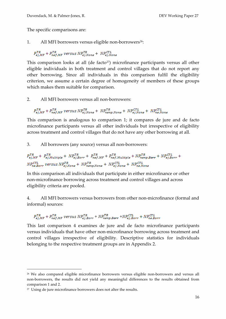
The specific comparisons are: 1. All MFI borrowers versus eligible non-borrowers26
:
This comparison looks at all (de facto27
) microfinance participants versus all other eligible individuals in both treatment and control villages that do not report any other borrowing. Since all individuals in this comparison fulfil the eligibility criterion, we assume a certain degree of homogeneity of members of these groups which makes them suitable for comparison.
2. All MFI borrowers versus all non-borrowers:
This comparison is analogous to comparison 1; it compares de jure and de facto microfinance participants versus all other individuals but irrespective of eligibility across treatment and control villages that do not have any other borrowing at all. 3. All borrowers (any source) versus all non-borrowers:
In this comparison all individuals that participate in either microfinance or other non-microfinance borrowing across treatment and control villages and across eligibility criteria are pooled. 4. All MFI borrowers versus borrowers from other non-microfinance (formal and informal) sources:
+ +
This last comparison 4 examines de jure and de facto microfinance participants versus individuals that have other non-microfinance borrowing across treatment and control villages irrespective of eligibility. Descriptive statistics for individuals belonging to the respective treatment groups are in Appendix 2.
26 We also compared eligible microfinance borrowers versus eligible non-borrowers and versus all non-borrowers, the results did not yield any meaningful differences to the results obtained from comparison 1 and 2. 27 Using de jure microfinance borrowers does not alter the results.
Duvendack, M. & Palmer-Jones, R. DEV Working Paper 27
17
As mentioned earlier, PnK find microcredit is more effective when women are involved. We also provide separate impact estimates for women and men separately28
.
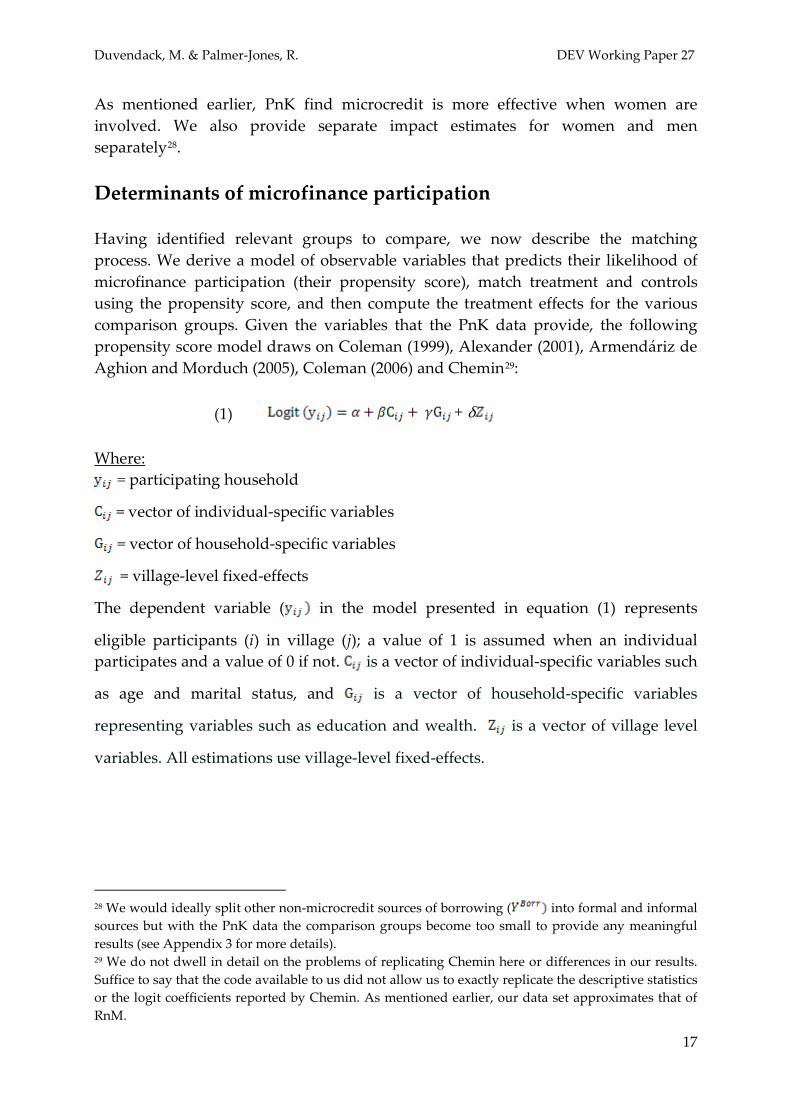
Determinants of microfinance participation Having identified relevant groups to compare, we now describe the matching process. We derive a model of observable variables that predicts their likelihood of microfinance participation (their propensity score), match treatment and controls using the propensity score, and then compute the treatment effects for the various comparison groups. Given the variables that the PnK data provide, the following propensity score model draws on Coleman (1999), Alexander (2001), Armendáriz de Aghion and Morduch (2005), Coleman (2006) and Chemin29
:
(1) + δ
Where: = participating household
= vector of individual-specific variables
= vector of household-specific variables
= village-level fixed-effects
The dependent variable ( in the model presented in equation (1) represents
eligible participants (i) in village (j); a value of 1 is assumed when an individual participates and a value of 0 if not. is a vector of individual-specific variables such
as age and marital status, and is a vector of household-specific variables
representing variables such as education and wealth. is a vector of village level
variables. All estimations use village-level fixed-effects.
28 We would ideally split other non-microcredit sources of borrowing ( into formal and informal sources but with the PnK data the comparison groups become too small to provide any meaningful results (see Appendix 3 for more details). 29 We do not dwell in detail on the problems of replicating Chemin here or differences in our results. Suffice to say that the code available to us did not allow us to exactly replicate the descriptive statistics or the logit coefficients reported by Chemin. As mentioned earlier, our data set approximates that of RnM.

Duvendack, M. & Palmer-Jones, R. DEV Working Paper 27
18
Table 1: Logistic regression model for all four treatment groups across treatment and control villages and across eligibility criteria
Independent variables
Sex HH head (male=1) 0.836*** 0.792*** -0.472 0.656***
0.000 0.000 -0.333 -0.001
Age (years) 0.007** 0.008*** 0.044*** 0.021***
-0.025 -0.008 0.000 0.000
Age household head -0.007* -0.010** -0.024*** -0.015*** (years) -0.081 -0.014 0.000 0.000 Number adult male in -0.270*** -0.260*** -0.175** -0.221*** household 0.000 0.000 -0.039 0.000 Marital status (yes=1) 1.173*** 1.179*** 2.029*** 1.472***
0.000 0.000 0.000 0.000
Highest education of any 0.007 0.010 0.070*** 0.035*** household member -0.615 -0.470 -0.001 -0.005 Highest education any
-0.069*** -0.074*** 0.022 -0.043***
female household
0.000 0.000 -0.352 -0.007 Livestock value -0.000** -0.000* 0.000 0.000
-0.031 -0.063 -0.417 -0.210
Own non-farm enterprise 0.322*** 0.324*** 0.050 0.263*** (yes=1) 0.000 0.000 -0.666 0.000 Household size -0.041* -0.046** 0.005 -0.032*
-0.081 -0.042 -0.875 -0.099
Village dummies Yes Yes Yes Yes Number of observations 5436 5436 5436 5436 Pseudo R-squared 0.125 0.129 0.135 0.103 Source: Authors calculations. For differences with Chemin, see footnote 29. Notes: p-values in italics. * significant at 10%, ** significant at 5%, *** significant at 1%. Using PnK data, see footnote 8. Control variables such as savings, landholdings of household head’s parents and landholdings of household head’s brothers were included, all insignificant. Descriptive statistics for all four treatment groups can be found in Appendix 2. Table 1 shows that the main variables that are statistically significant across all four treatment groups are age, age of household head, number of adult males in the household and marital status. Highest education of any female household member, ownership of a non-farm enterprise, sex of household head and household size are statistically significant across . However, the sign of the
coefficients and the level of significance vary from group to group. Further, note that the pseudo R-squared for the various models is rather low ranging from 0.103 to 0.135 (and lower than reported by Chemin).

Duvendack, M. & Palmer-Jones, R. DEV Working Paper 27
19
Treatment group results As mentioned above, the basic idea of matching is to compare a participant with one or more non-participants who are similar in terms of a set of observed covariates X (Caliendo and Kopeinig, 2005; 2008). This requires predicting propensity scores for each individual, that is participants as well as non-participants using a logit or a probit model. We used the logit model presented in Table 1. Before implementing the actual matching process, we examine whether the common support assumption is satisfied. Where the densities of the estimated propensity scores for participants and non-participants overlap reasonably well, the common support assumption is met (Abou-Ali et al, 2009). Figure 3 presents the density of propensity scores, indicating somewhat different densities for participants (YMF) and non-participants (YNone) (pooling treatment and control villages). This implies that many households would not be good matches as the density of propensity scores of potential controls occurs at low propensity scores while than of treatment households are at high propensity scores30
30 This is further explored in Appendix 4.
. Graphs (not shown) for other comparisons are similar even when using only de jure eligible persons.

Duvendack, M. & Palmer-Jones, R. DEV Working Paper 27
20
Figure 2: Distribution of propensity scores for participants (YMF) and non-participants (YNone
) (comparison 2), all villages
Source: Authors calculations. Table 2 and Table 3 present the differences in the outcome variables for participants and their matched non-participants for all four comparisons described earlier. Table 2 illustrates the impact estimates for microcredit participation for all participants (male and female together) while Table 3 provides impact estimates for male and female participants separately. Two different matching algorithms were applied, nearest neighbour matching with replacement31, and kernel matching using three different bandwidths (0.01, 0.02 and 0.05), to assess the degree of variability of the different matching results across algorithms32
.
The distributions of the covariates for the treatment and controls need to be similar, that is balanced (Abou-Ali et al, 2009). Our comparisons all pass balancing tests33
31 This allows a control household to match to more than one treatment household.
,
32 The literature on the choice of matching algorithms is not yet very developed. Morgan and Winship (2007: 109) argue that kernel matching, introduced by Heckman et al (1998) and Heckman, Ichimura and Todd (1998) appears to be the most efficient and preferred algorithm. Nearest neighbour matching was chosen for its popularity, which is probably due to it being easy to understand and easy to implement. We present only the kernel matching estimates with a bandwidth of 0.05. All other results can be obtained from the authors. 33 The Stata command pstest was used.
0 .2 .4 .6 Value of Propensity Score
Non-participants Participants
Den
sity

Duvendack, M. & Palmer-Jones, R. DEV Working Paper 27
21
although the differences between treatment and control group means were reduced considerably by matching in most cases. Table 2: Simple matching estimates across gender using kernel matching bandwidth 0.05 for all four comparison groups
Outcome variables vs eligible
vs
+ vs vs
Comparison 1 2 3 4 Kernel matching, 0.0534
Variation of log per capita expenditure
(Taka) -0.014** -0.014** -0.001 -0.034*
Log per capita expenditure (Taka) -0.019 -0.011 0.019 -0.089**
Log women non-landed assets (Taka) 1.036*** 0.498*** 0.349** -0.022
Female labour supply, aged 16-59, hours per
month 52.63*** 57.81*** 31.86*** 78.43***
Male labour supply, aged 16-59, hours per
month -30.33** -47.06*** 40.00*** -276.22***
Girl school enrolment, aged 5-17 years 0.053* 0.060* 0.061** 0.077
Boy school enrolment, aged 5-17 years 0.027 0.035 0.060** -0.011
Source: Authors calculations. Notes: *statistically significant at 10%, **statistically significant at 5%, ***statistically significant at 1%. Using PnK data, see footnote 8. Stata routine psmatch235
using the logit model outlined in Table 1 is used. Standard errors (not reported) are bootstrapped.
The results in Table 2 are rather mixed, with different comparisons showing different levels of significance for different outcome variables. When comparing versus all
eligible and not eligible (comparison 2), microcredit participation appears to
significantly improve women’s non-landed assets, female labour supply and girls’ school enrolment, for example female microfinance participants appear to work 57 hours more per month (presumed benefit) than non-participants. However, when 34 1-nearest neighbour matching as well as kernel matching with bandwidth 0.01 and 0.02 were applied in addition to 0.05 but the various algorithms and bandwidths results did not differ significantly and thus only the results using a bandwidth of 0.05 are shown here. 35 Robustness checks were conducted using different Stata routines including psmatch2 (Leuven and Sianesi, 2003), and pscore (Becker and Ichino, 2002). The results obtained did not vary significantly.

Duvendack, M. & Palmer-Jones, R. DEV Working Paper 27
22
directly comparing microfinance participants with participants in other non-microfinance financing schemes (comparison 4), microfinance participants do worse than non-microfinance borrowers in terms of log of per capita expenditure and the variation thereof. Comparison 1, versus eligible , suggests that microcredit
participation has significant negative impacts on the variation of the log of per capita expenditure, but that it significantly improves women’s non-landed assets, female labour supply and girls’ school enrolment. However, most other outcome variables remain insignificant within this comparison. Comparison 3 indicates significant positive impacts on all outcome variables except the log of per capita expenditure and its variation which are insignificant, implying that microfinance in combination with other forms of finance makes a bigger difference to the lives of the poor. The results above recur for women’s borrowing (see Table 3). It seems that microfinance participation has an apparently significant positive impact on female related outcome variables such as women’s non-landed assets, female labour supply and partially on girls’ school enrolment (see comparisons 1, 2 and 3). However, there are little significant effects on the remaining variables. Noteworthy are the significantly negative impacts of microfinance participation on the log of per capita expenditure and the variation thereof as indicated by comparisons 1, 2 and 4 in Table 2 and Table 3; this is in contrast to PnK’s headline findings.

Duvendack, M. & Palmer-Jones, R. DEV Working Paper 27
23
Table 3: Matching estimates of impact by gender (kernel matching bandwidth 0.05 for all four comparison groups)
Outcome variables vs
eligible
vs
+ vs
vs
Comparison 1 2 3 4
Kernel matching, 0.0536
Variation of log per capita expenditure
(Taka)
Women -0.017** -0.016* -0.009 -0.047
Men -0.017** -0.030*** -0.001 -0.039*
Log per capita expenditure (Taka)
Women -0.019 -0.013 0.012 -0.126*
Men -0.021 -0.046** 0.015 -0.079**
Log women non-landed assets (Taka)
Women 1.009*** 0.754*** 0.561*** -0.848
Men 1.297*** -0.000 0.244 0.249
Female labour supply, aged 16-59, hours per
month
Women 54.42*** 101.64*** 54.71*** 32.77
Men -43.74*** -42.02*** 30.85*** 93.03***
Male labour supply, aged 16-59, hours per
month
Women -51.80*** -257.41***
-49.52*** -83.27
Men 18.42 401.30*** 49.83*** -329.40***
Girl school enrolment, aged 5-17 years
Women 0.040 0.067* 0.061** -0.216
Men 0.097*** 0.032 0.060** 0.133
Boy school enrolment, aged 5-17 years
Women 0.029 0.045 0.050 -0.128
Men 0.039 -0.001 0.054** -0.017 Source: Authors calculations. Notes: Notes: *statistically significant at 10%, **statistically significant at 5%, ***statistically significant at 1%. Using PnK data, see footnote 8. Stata routine psmatch237
using the logit model outlined in Table 1 is used. Standard errors (not reported) are bootstrapped.
36 As in the case of the results presented in Table 2, 1-nearest neighbour matching as well as kernel matching with bandwidth 0.01 and 0.02 were applied in addition to 0.05 but the various algorithms and bandwidths results did not differ significantly and thus only the results using a bandwidth of 0.05 are shown here. 37 As before, robustness checks were conducted using different Stata routines. The results obtained did not vary significantly.

Duvendack, M. & Palmer-Jones, R. DEV Working Paper 27
24
To conclude, the findings presented in Table 2 and Table 3 are mixed and it is not obvious that microcredit participation is associated with more significant impacts than participation in other non-microcredit sources of borrowing. Comparison 3 which looks at + versus all eligible and not eligible
suggests that microfinance in combination with other forms of finance makes a real difference, while microfinance alone compared to other sources of finance ( has mixed or even significantly negative impacts (comparison 4).
The results in Table 2 provide evidence that participation in both microcredit and other sources of borrowing is associated with significant positive effects for some outcome variables. It appears that any form of finance – microcredit, formal or informal borrowing - can be associated with higher well-being of participating households. However, when examining the results by gender (see Table 3), we find that impacts for male labour supply is greater in the case of male borrowing (and female labour supply falls). Similarly the impact of female labour supply is greater for women in the case of female borrowing (and male labour supply falls). To summarise our arguments so far; relatively few households served as matches as illustrated by Figure 3 and further explored in Appendix 4. This raises the question of the suitability of PSM in the context of PnK. The PnK data set has very few households in control villages (n=260), many of which are not likely matches not least because of because large differences in landholdings makes them ‘not eligible’. There are relatively few non-borrowing eligible households in treatment villages, and anyway these are likely different in significant ways to microfinance borrowers by the very fact that they are not microfinance borrowers although they could have been. This is a limitation of the sampling strategy described above, and is a major drawback since PSM works best when there are more control than treatment households (Smith and Todd, 2005). Moreover, a rich and high quality data set is required to optimise results (Smith and Todd, 2005), which appears not to be the case here. Sensitivity analysis on treatment group comparisons Although significant effects are found using PSM it is questionable whether these are robust to unobservables because PSM cannot control for unobservable characteristics. Rosenbaum (2002) developed sensitivity analysis to explore the robustness of matching estimates to selection on unobservables (Rosenbaum, 2002). Ichino, Mealli and Nannicini (2006) argue that ‘sensitivity analysis should always accompany the presentation of matching estimates’ (19).
Duvendack, M. & Palmer-Jones, R. DEV Working Paper 27
25
Rosenbaum (2002) invites us to imagine a number Γ (gamma) 1) which captures
the degree of association, of an unobserved characteristic with the treatment and outcome, required for it (the unobserved characteristic) to explain the observed impact. Γ is the ratio of the odds38
that the treated have this unobserved characteristic to the odds that the controls have it; a low odds ratio (near to one) indicates that it is not unlikely that such an unobserved variable exists. Cornfield et al (1959) use the example of the effect of smoking on lung cancer. In this case, which is now surely without doubt, data from the late 1950s gives a gamma > 5 for such an unobserved variable, which is, it is suggested, highly unlikely to have been unobserved because of its strong association between smoking and death.
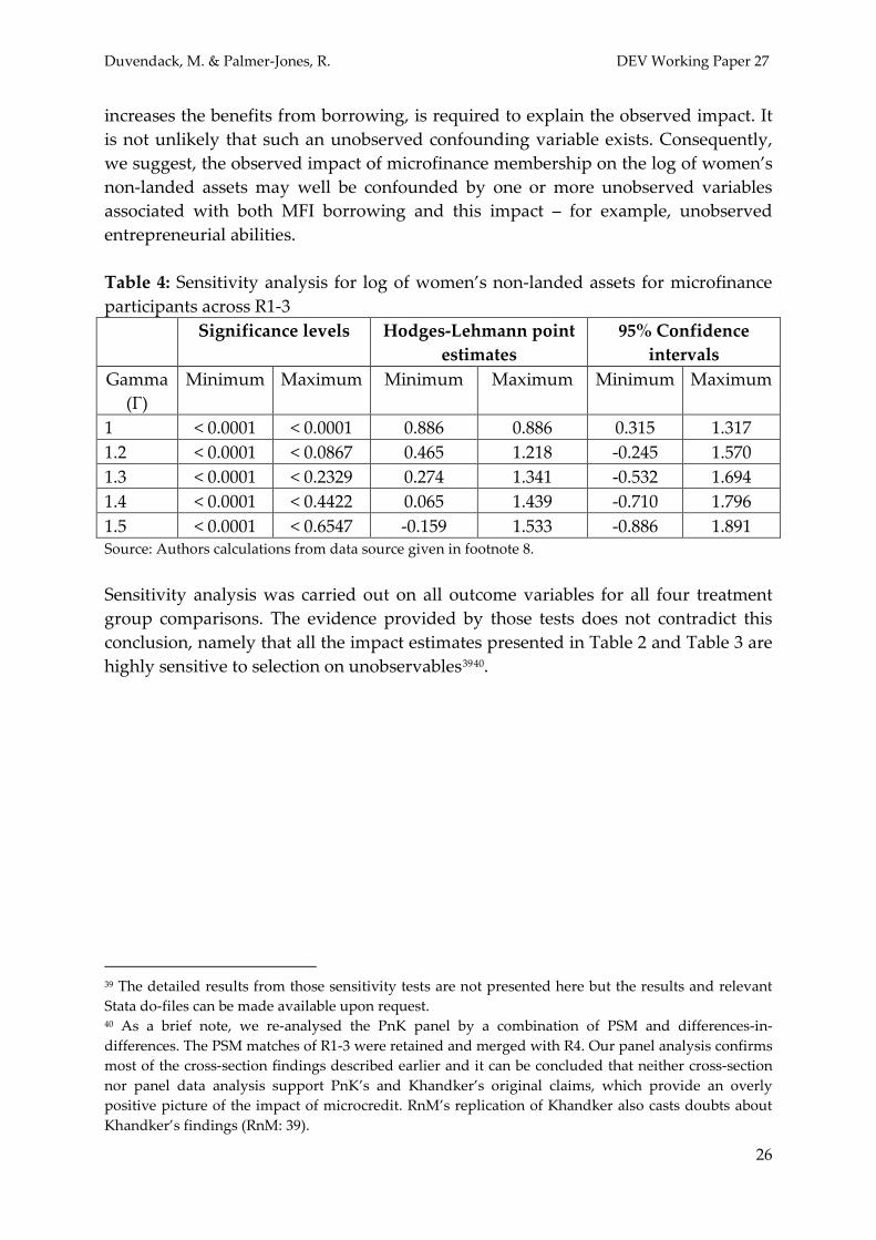
This approach can be implemented using the rbounds procedure in Stata (Becker and Caliendo, 2007); this procedure uses the matching estimates to calculate the confidence intervals (for a given level of confidence – for example 95%) of the outcome variable for different values of Γ. A value of Γ that produces a confidence interval that encompasses zero is one that would make the estimated impact not statistically significant at the relevant level of confidence. If the lowest Γ (which encompasses zero) is relatively small (say < 2) then one may assert that the likelihood of such an unobserved characteristic is relatively high and therefore that the estimated impact is rather sensitive to the existence of unobservables (DiPrete and Gangl, 2004). Conversely, if the value of Γ that produces a confidence interval encompassing zero is large (say > 5) then it is rather unlikely that such a variable would not have been discovered, since its association with the outcome is so high. In this case one can say that the effect is rather robust to unobservables, and it appears unlikely that such a confounding variable would not have been observed. Sensitivity analysis can be illustra ted by calcula ting the Γ a t which the estima ted impact of microfinance participation on the log of women’s non-landed assets for comparison 2 is no longer statistically significant. Table 2 shows that the kernel matching impact estimate with a bandwidth of 0.05 for the log of women’s non-landed assets is 0.498 which is statistically significant at 1%. However, this may not be due to membership per se but to unobserved characteristics that account for membership (and or its impact). Sensitivity analysis explores the vulnerability of this impact estimate to selection on unobservables. Table 4 reports the rbounds results, showing that when Γ = 1.2, a relatively small difference in the odds of exposure, or more, the 95% confidence interval of the point impact estimates encompasses zero; at gamma = 1.5 the Hodges-Lehmann point estimates encompass zero. This implies that a relatively small increase in the likelihood of being a participant due to an unobservable characteristic which also 38 Odds, which are widely used in assessing probabilistic outcomes, are derived from probabilities (0 ≤
≤ 1) by the following formula: .
Duvendack, M. & Palmer-Jones, R. DEV Working Paper 27
26
increases the benefits from borrowing, is required to explain the observed impact. It is not unlikely that such an unobserved confounding variable exists. Consequently, we suggest, the observed impact of microfinance membership on the log of women’s non-landed assets may well be confounded by one or more unobserved variables associated with both MFI borrowing and this impact – for example, unobserved entrepreneurial abilities. Table 4: Sensitivity analysis for log of women’s non-landed assets for microfinance participants across R1-3 Significance levels Hodges-Lehmann point
estimates 95% Confidence
intervals Gamma
(Γ) Minimum Maximum Minimum Maximum Minimum Maximum
1 < 0.0001 < 0.0001 0.886 0.886 0.315 1.317 1.2 < 0.0001 < 0.0867 0.465 1.218 -0.245 1.570 1.3 < 0.0001 < 0.2329 0.274 1.341 -0.532 1.694 1.4 < 0.0001 < 0.4422 0.065 1.439 -0.710 1.796 1.5 < 0.0001 < 0.6547 -0.159 1.533 -0.886 1.891 Source: Authors calculations from data source given in footnote 8. Sensitivity analysis was carried out on all outcome variables for all four treatment group comparisons. The evidence provided by those tests does not contradict this conclusion, namely that all the impact estimates presented in Table 2 and Table 3 are highly sensitive to selection on unobservables3940
39 The detailed results from those sensitivity tests are not presented here but the results and relevant Stata do-files can be made available upon request.
.
40 As a brief note, we re-analysed the PnK panel by a combination of PSM and differences-in-differences. The PSM matches of R1-3 were retained and merged with R4. Our panel analysis confirms most of the cross-section findings described earlier and it can be concluded that neither cross-section nor panel data analysis support PnK’s and Khandker’s original claims, which provide an overly positive picture of the impact of microcredit. RnM’s replication of Khandker also casts doubts about Khandker’s findings (RnM: 39).

Duvendack, M. & Palmer-Jones, R. DEV Working Paper 27
27
Conclusion The replication of PnK and associated studies poses a challenge due to the complex research design and poor documentation of the data. All studies that deal with the PnK data, that is Morduch, Chemin, RnM and this study, agree that PnK overstate the impacts of microcredit. PnK estimated positive and significant impacts for literally all of the six outcome variables with stronger impacts when women were involved in microcredit (PnK: 987-988). Morduch argued that PnK overestimated the impact of microcredit in part because the eligibility criterion was not strictly enforced, and he cannot support PnK’s claims that microcredit increases per capita expenditure, school enrolment for children (Morduch: 30) or labour supply. Pitt challenged Morduch’s conclusions with simulated data, and confirms the results of PnK’s undocumented and undocumentable estimation procedure. RnM confute Pitt’s claims with their (available) data and documented computer code. Using PSM, Chemin finds lower impact estimates than PnK for all outcome variables except male labour supply (Chemin: 478). Doubts about both Morduch and Chemin arise because of problems in replicating their data constructions, and in the latter case the failure to conduct sensitivity analysis. RnM’s findings of MFI impact are mixed and mostly insignificant. The studies by PnK, Morduch, Chemin and RnM do not address the role of multiple sources of borrowing41
which has implications for the nature and constitution of the treatment and control groups. As a result, this study, using PSM with sensitivity analysis, made different comparisons to examine impacts using putatively more appropriate, and homogeneous, treatment and control groups. This strategy found generally positive but mixed results when comparing microcredit participation with non-participation, but there is no clear evidence that microcredit as such is more beneficial than other sources of finance; moreover, sensitivity analysis shows that all these estimates of impact are highly vulnerable to unobservables, in part, perhaps, because of the poor quality of the matches.
Many microfinance adepts agree that individuals essentially need to borrow from multiple sources to obtain sufficient funds that would allow them to engage in more productive activities (see Fernando, 1997); microcredit loans are often too small to meet the needs of microentrepreneurs (Venkata and Yamini, 2010). In addition, multiple sources of borrowing are often required to smooth income and consumption patterns as well as to cope with emergencies (Venkata and Yamini, 2010). Fernando (1997), Coleman (1999) and Venkata and Yamini (2010) find that it is common for individuals to use borrowing from one source to pay off the loans of another, including microfinance, on time. 41 Khandker (2000) only explores the effects of other borrowing sources on a limited set of variables.

Duvendack, M. & Palmer-Jones, R. DEV Working Paper 27
28
Criticisms of the more strident and unqualified claims about microfinance (using RCTs) are becoming more common (Banerjee et al, 2009; RnM; Karlan and Zinman, 2009) and further investigations as to the impact of microcredit versus other financial tools should be encouraged, whether RCTs or carefully designed observational studies that collect a rich and high quality data set. It is arguable that carefully conducted observational studies using quasi-experimental designs can and perhaps should have come to the appropriate conclusions, and could have done so with even these data had the data manipulation and analysis been appropriate, without the need to engage in RCTs (for a critique on RCTs see Deaton, 2009; Imbens, 2009; Pritchett, 2009). The analysis in this paper has raised doubts about the capabilities of PSM, to rescue robust estimates of impact, at least with the sorts of data available. A critique of econometric techniques is not new; in a landmark paper Leamer (1983) criticises the key assumptions many econometric methods are built on and complains about ‘the whimsical character of econometric inference’ (38). Despite his pessimistic view on the usefulness of econometric methods, there has been a trend towards ever more sophisticated techniques which, however, do not necessarily provide convincing solutions to the challenges of impact evaluation. A similar conclusion would seem to apply to PSM.
Duvendack, M. & Palmer-Jones, R. DEV Working Paper 27
29
References Abou-Ali, H., El-Azony, H., El-Laithy, H., Haughton, J. and Khandker, S. R. (2009)
Evaluating the Impact of Egyptian Social Fund for Development Programs. World Bank Policy Research Working Paper No. 4993, July.
Alexander, G. (2001) An Empirical Analysis of Microfinance: Who are the Clients? Northeastern Universities Development Consortium Conference. Boston, 28-30 September 2001.
Armendáriz de Aghion, B. and Morduch, J. (2005) The Economics of Microfinance. Cambridge: MIT Press.
Armendáriz de Aghion, B. and Morduch, J. (2010) The Economics of Microfinance. 2nd
Banerjee, A., Duflo, E., Glennerster, R. and Kinnan, C. (2009). The Miracle of Microfinance? Evidence from a Randomized Evaluation. Available at: http://econ-www.mit.edu/files/4162.
ed. Cambridge: MIT Press.
Bangladesh Bureau of Statistics (1985) Statistical Yearbook of Bangladesh 1984-85. Dhaka: People's Republic of Bangladesh.
Bangladesh Bureau of Statistics (2004) Statistical Yearbook of Bangladesh 2004. Dhaka: People's Republic of Bangladesh.
Bateman, M. and Chang, H.-J. (2009) The Microfinance Illusion. Available at: http://www.econ.cam.ac.uk/faculty/chang/pubs/Microfinance.pdf.
Becker, S. O. and Caliendo, M. (2007) Sensitivity Analysis for Average Treatment Effects. The STATA Journal, 7 (1), pp.71-83.
Becker, S. O. and Ichino, A. (2002). Estimation of Average Treatment Effects Based on Propensity Scores. The STATA Journal, 2 (4), pp.358-377.
Caliendo, M. and Hujer, R. (2005) The Microeconometric Estimation of Treatment Effects - An Overview. Forschungsinstitut zur Zukunft der Arbeit (IZA) Discussion Paper No. 1653, July.
Caliendo, M. and Kopeinig, S. (2005) Some Practical Guidance for the Implementation of Propensity Score Matching. Forschungsinstitut zur Zukunft der Arbeit (IZA) Discussion Paper No. 1588, May.
Caliendo, M. and Kopeinig, S. (2008) Some Practical Guidance for the Implementation of Propensity Score Matching. Journal of Economic Surveys, 22 (1), pp.31-72.
Chemin, M. (2008) The Benefits and Costs of Microfinance: Evidence from Bangladesh. Journal of Development Studies, 44 (4), pp.463-484.
Coleman, B. E. (1999) The Impact of Group Lending in Northeast Thailand. Journal of Development Economics, 60 (1), pp.105-141.
Coleman, B. E. (2006) Microfinance in Northeast Thailand: Who Benefits and How Much? World Development, 34 (9), pp.1612-1638.

Duvendack, M. & Palmer-Jones, R. DEV Working Paper 27
30
Cornfield, J., Haenszel, W., Hammond, E. and Lilienfeld, A. (1959) Smoking and Lung Cancer: Recent Evidence and a Discussion of Some Questions. Journal of the National Cancer Institute, 22, pp.173-203.
Deaton, A. (2009) Instruments of Development: Randomization in the Tropics, and the Search for the Elusive Keys to Economic Development. Available at: http://www.princeton.edu/~deaton/downloads/Instruments_of_Development.pdf.
Dichter, T. and Harper, M. eds. (2007) What's Wrong with Microfinance? Warwickshire: Practical Action Publishing.
DiPrete, T. A. and Gangl, M. (2004) Assessing Bias in the Estimation of Causal Effects: Rosenbaum Bounds on Matching Estimators and Instrumental Variables Estimation with Imperfect Instruments. Sociological Methodology, 34 (1), pp.271-310.
Fernando, J. L. (1997) Nongovernmental Organizations, Micro-Credit, and Empowerment of Women. The ANNALS of the American Academy of Political and Social Science, 554 (1), pp.150-177.
Gaile, G. L. and Foster, J. (1996) Review of Methodological Approaches to the Study of the Impact of Microenterprise Credit Programs. Report submitted to USAID Assessing the Impact of Microenterprise Services (AIMS), June.
Goetz, A. M. and Sen Gupta, R. (1996) Who Takes the Credit? Gender, Power, and Control Over Loan Use in Rural Credit Programs in Bangladesh. World Development, 24 (1), pp.45-63.
Goldberg, N. (2005) Measuring the Impact of Microfinance: Taking Stock of What We Know. Grameen Foundation USA Publication Series, December.
Hamermesh, D. S. (2007) Viewpoint: Replication in Economics. Canadian Journal of Economics, 40 (3), pp.715-733.
Heckman, J. J. (1979) Sample Selection Bias as a Specification Error. Econometrica, 47 (1), pp.153-161.
Heckman, J. J., Ichimura, H., Smith, J. and Todd, P. (1998) Characterizing Selection Bias Using Experimental Data. Econometrica, 66 (5), pp.1017-1098.
Heckman, J. J., Ichimura, H. and Todd, P. (1998) Matching as an Econometric Evaluation Estimator. The Review of Economic Studies, 65 (2), pp.261-294.
Hulme, D. and Mosley, P. (1996) Finance against Poverty. London: Routledge. Ichino, A., Mealli, F. and Nannicini, T. (2006) From Temporary Help Jobs to
Permanent Employment: What Can We Learn from Matching Estimators and their Sensitivity? Forschungsinstitut zur Zukunft der Arbeit (IZA) Discussion Paper No. 2149, May.
Imbens, G. (2009) Better LATE Than Nothing: Some Comments on Deaton (2009) and Heckman and Urzua (2009). NBER Working Paper No. 14896.
Karlan, D. and Zinman, J. (2009) Expanding Microenterprise Credit Access: Using Randomized Supply Decisions to Estimate the Impacts in Manila. Available at: http://karlan.yale.edu/p/expandingaccess_manila_jul09.pdf.
Khandker, S. R. (1996) Role of Targeted Credit in Rural Non-farm Growth. Bangladesh Development Studies, 24 (3 & 4).

Duvendack, M. & Palmer-Jones, R. DEV Working Paper 27
31
Khandker, S. R. (1998) Fighting Poverty with Microcredit: Experience in Bangladesh. New York: Oxford University Press.
Khandker, S. R. (2000) Savings, Informal Borrowing and Microfinance. Bangladesh Development Studies, 26 (2 & 3).
Khandker, S. R. (2005) Microfinance and Poverty: Evidence Using Panel Data from Bangladesh. The World Bank Economic Review, 19 (2), pp.263-286.
Leamer, E. E. (1983) Let's Take the Con Out of Econometrics. The American Economic Review, 73 (1), pp.31-43.
Leuven, E. and Sianesi, B. (2003) PSMATCH2: STATA Module to Perform Full Mahalanobis and Propensity Score Matching, Common Support Graphing, and Covariate Imbalance Matching. Available at: http://ideas.repec.org/c/boc/bocode/s432001.html.
McKernan, S.-M. (2002) The Impact of Microcredit Programs on Self-Employment Profits: Do Noncredit Program Aspects Matter? Review of Economics and Statistics, 84 (1), pp.93-115.
Menon, N. (2006) Non-linearities in Returns to Participation in Grameen Bank Programs. Journal of Development Studies, 42 (8), pp.1379 - 1400.
Morduch, J. (1998) Does Microfinance Really Help the Poor? New Evidence from Flagship Programs in Bangladesh. Unpublished mimeo.
Morduch, J. (1999) The Microfinance Promise. Journal of Economic Literature, XXXVII December, pp.1569-1614.
Morduch, J. and Haley, B. (2002) Analysis of the Effects of Microfinance on Poverty Reduction. NYU Wagner Working Paper No. 1014, June.
Morgan, S. L. and Winship, C. (2007) Counterfactuals and Causal Inference. Methods and Principles for Social Research. Cambridge: Cambridge University Press.
Nannicini, T. (2007) Simulation-based Sensitivity Analysis for Matching Estimators. The STATA Journal, 7 (3), pp.334-350.
Neyman, J. S. (1923) On the Application of Probability Theory to Agricultural Experiments. Essay on Principles. Section 9. Translated in Statistical Science, 5 (4), pp.465-480, 1990.
Odell, K. (2010) Measuring the Impact of Microfinance: Taking Another Look. Grameen Foundation USA Publication Series, May.
Pitt, M., Khandker, S. R. and Cartwright, J. (2006) Empowering Women with Micro-finance: Evidence from Bangladesh. Economic Development and Cultural Change, pp.791-831.
Pitt, M., Khandker, S. R., Chowdhury, O. H. and Millimet, D. L. (2003) Credit Programmes for the Poor and the Health Status of Children in Rural Bangladesh. International Economic Review, 44 (1), pp.87-118.
Pitt, M. M. (1999) Reply to Jonathan Morduch’s “Does Microfinance Really Help the Poor? New Evidence from Flagship Programs in Bangladesh”. Unpublished mimeo.
Pitt, M. M. (2000) The Effect of Nonagricultural Self-Employment Credit on Contractual Relations and Employment in Agriculture: The Case of

Duvendack, M. & Palmer-Jones, R. DEV Working Paper 27
32
Microcredit Programs in Bangladesh. Bangladesh Development Studies, 26 (2 & 3), pp.15-48.
Pitt, M. M. and Khandker, S. R. (1998) The Impact of Group-Based Credit Programs on Poor Households in Bangladesh: Does the Gender of Participants Matter? Journal of Political Economy, 106 (5), pp.958-996.
Pitt, M. M. and Khandker, S. R. (2002) Credit Programmes for the Poor and Seasonality in Rural Bangladesh. Journal of Development Studies, 39 (2), pp.1-24.
Pitt, M. M., Khandker, S. R., McKernan, S.-M. and Latif, M. A. (1999) Credit Programs for the Poor and Reproductive Behavior of Low-Income Countries: Are the Reported Causal Relationships the Result of Heterogeneity Bias? Demography, 36 (1), pp.1-21.
Pritchett, L. (2009) The Policy Irrelevance of the Economics of Education: Is "Normative as Positive" Just Useless, or Worse? In Cohen, J. and Easterly, W., eds. What Works in Development? Thinking Big and Thinking Small. Washington D.C.: Brookings Institution Press.
Ravallion, M. (2001) The Mystery of the Vanishing Benefits: An Introduction to Impact Evaluation. The World Bank Economic Review, 15 (1), pp.115-140.
Ravallion, M. (2008) Evaluating Anti-Poverty Programs. In Schultz, T. P. and Strauss, J., eds. Handbook of Development Economics, Volume 4. Amsterdam: Elsevier.
Roodman, D. and Morduch, J. (2009) The Impact of Microcredit on the Poor in Bangladesh: Revisiting the Evidence. Center for Global Development, Working Paper No. 174, June.
Rosenbaum, P. R. (2002) Observational Studies. New York: Springer. Rosenbaum, P. R. and Rubin, D. B. (1983) The Central Role of the Propensity Score in
Observational Studies for Causal Effects. Biometrika, 70 (1), pp.41-55. Rosenbaum, P. R. and Rubin, D. B. (1984) Reducing Bias in Observational Studies
Using Subclassification on the Propensity Score. Journal of the American Statistical Association, 79 (387), pp.516-524.
Rubin, D. B. (1973a) Matching to Remove Bias in Observational Studies. Biometrics, 29 (1), pp.159-183.
Rubin, D. B. (1973b) The Use of Matched Sampling and Regression Adjustment to Remove Bias in Observational Studies. Biometrics, 29 (1), pp.185-203.
Rubin, D. B. (1974) Estimating Causal Effects of Treatments in Randomized and Nonrandomized Studies. Journal of Educational Psychology, 66 (5), pp.688-701.
Rubin, D. B. (1977) Assignment to Treatment Group on the Basis of a Covariate. Journal of Educational Statistics, 2 (1), pp.1-26.
Rubin, D. B. (1978) Bayesian Inference for Causal Effects: The Role of Randomization. The Annals of Statistics, 6 (1), pp.34-58.
Rutherford, S. (2001) The Poor and Their Money. New Delhi: Oxford University Press. Sebstad, J. and Chen, G. (1996) Overview of Studies on the Impact of Microenterprise
Credit. Report submitted to USAID Assessing the Impact of Microenterprise Services (AIMS), June.
Duvendack, M. & Palmer-Jones, R. DEV Working Paper 27
33
Smith, J. A. and Todd, P. (2005) Does Matching Overcome LaLonde's Critique of Nonexperimental Estimators? Journal of Econometrics, 125, pp.305-353.
Venkata, N. A. and Yamini, V. (2010) Why Do Microfinance Clients Take Multiple Loans? MicroSave India Focus Note 33, February.
Yunus, M. (1999) Banker to the Poor: Micro-Lending and the Battle Against World Poverty. New York: PublicAffairs.

Duvendack, M. & Palmer-Jones, R. DEV Working Paper 27
34
Appendix Appendix 1: Weighted means and standard deviations, PnK and RnM
Variables PnK 1998 RnM 20091 2
Mean Standard deviation
Mean Standard deviation
Age of all individuals 23 18 23 18 Schooling of individual aged 5 or above (years)
1.377 2.773 2.066 3.136
Parents of HH head own land? 0.256 0.564 0.254 0.563 Brothers of HH head own land? 0.815 1.308 0.810 1.305 Sisters of HH head own land? 0.755 1.208 0.750 1.206 Parents of HH head’s spouse own land? 0.529 0.784 0.529 0.783 Brothers of HH head’s spouse own land? 0.919 1.427 0.919 1.427 Sisters of HH head’s spouse own land? 0.753 1.202 0.753 1.202 Household land (decimals) 76.142 108.540 76.145 108.052 Highest grade completed by HH head 2.486 3.501 2.523 3.525 Sex of household head (male=1) 0.948 0.223 0.948 0.223 Age of household head (years) 40.821 12.795 40.874 12.789 Highest grade completed by any female HH member
1.606 2.853 1.664 2.999
Highest grade completed by any male HH member
3.082 3.081 3.277 4.016
Adult female not present in HH? 0.017 0.129 0.017 0.129 Adult male not present in HH? 0.035 0.185 0.035 0.185 Spouse not present in HH? 0.126 0.332 0.123 0.329 Amount borrowed by female from BRAC (Taka)
350 1,574 349 1,564
Amount borrowed by male from BRAC (Taka)
172 1,565 173 1,575
Amount borrowed by female from BRDB (Taka)
114 747 114 746
Amount borrowed by male from BRDB (Taka)
203 1,573 204 1,576
Amount borrowed by female from GB (Taka) 956 4,293 972 4,324 Amount borrowed by male from GB (Taka) 374 2.923 360 2,895 Notes: 1. Source: PnK, table A1, p. 993, based on R1. 2. Source: RnM, table 1, p. 15, based on R1. Morduch and Pitt do not provide any descriptive statistics.
Duvendack, M. & Palmer-Jones, R. DEV Working Paper 27
35
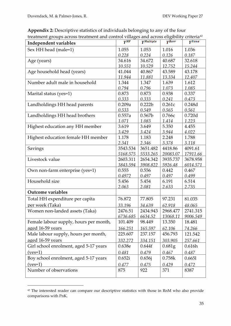
Appendix 2: Descriptive statistics of individuals belonging to any of the four treatment groups across treatment and control villages and across eligibility criteria42
Independent variables
Sex HH head (male=1) 1.055 1.053 1.016 1.036 0.228 0.224 0.126 0.187
Age (years) 34.616 34.672 40.687 32.618 10.551 10.529 12.752 15.244
Age household head (years) 41.044 40.867 43.589 43.178 11.944 11.881 13.334 12.407
Number adult male in household 1.344 1.347 1.639 1.612 0.794 0.796 1.073 1.085
Marital status (yes=1) 0.873 0.873 0.938 0.337 0.333 0.333 0.241 0.473
Landholdings HH head parents 0.209a 0.222b 0.261c 0.248d 0.533 0.549 0.565 0.561
Landholdings HH head brothers 0.557a 0.567b 0.766c 0.720d 1.071 1.083 1.414 1.223
Highest education any HH member 3.619 3.649 5.350 4.455 3.429 3.424 3.944 4.022
Highest education female HH member 1.178 1.183 2.248 1.788 2.341 2.346 3.378 3.118
Savings 3543.534 3651.482 4418.86 4091.61 5168.575 5533.265 20083.07 17911.66
Livestock value 2603.311 2654.342 3935.737 3678.958 3843.594 3908.822 5926.48 6014.571
Own non-farm enterprise (yes=1) 0.555 0.556 0.442 0.467 0.4972 0.497 0.497 0.499
Household size 5.456 5.454 6.191 6.514 2.063 2.081 2.633 2.735
Outcome variables Total HH expenditure per capita
per week (Taka) 76.872 77.805 97.231 81.035 33.196 34.639 62.918 48.065
Women non-landed assets (Taka) 2476.51 2434.943 2968.477 2741.315 6736.685 6634.52 13068.11 9006.549
Female labour supply, hours per month, aged 16-59 years
101.409 98.449 13.350 18.481 166.251 165.597 62.106 74.266
Male labour supply, hours per month, aged 16-59 years
225.607 237.157 456.793 121.542 332.272 334.151 303.905 257.661
Girl school enrolment, aged 5-17 years (yes=1)
0.638e 0.644f 0.681g 0.616h 0.481 0.479 0.467 0.487
Boy school enrolment, aged 5-17 years (yes=1)
0.652i 0.656j 0.758k 0.665l 0.477 0.475 0.429 0.472
Number of observations 875 922 371 8387
42 The interested reader can compare our descriptive statistics with those in RnM who also provide comparisons with PnK.

Duvendack, M. & Palmer-Jones, R. DEV Working Paper 27
36
Source: Authors calculations. Notes: Standard deviation in italics. Using PnK data, see footnote 8. MF=Participant in microfinance only; Multiple=Participant in microfinance and other non-microfinance (formal/informal) borrowing; Borr=Participant in other non-microfinance (formal/informal) borrowing; None=No borrowing at all. • a: n = 861; b: n = 908; c: n = 368; d: n = 8278 • e: n = 516; f: n = 542; g: n = 232; h: n = 5621 • i: n = 554; j: n = 582; k: n = 248; l: n = 5769 The mean values in Appendix 2 differ from the mean values presented by PnK and RnM as illustrated in Appendix 1. ANOVA has been applied examining all possible pairwise comparisons to assess whether the differences in the mean values between the various comparison groups are statistically significant. The ANOVA results show that for most variables differences are not significant at conventional levels of significance, with few exceptions. Mean values of versus
significantly differ for age of household head, landholdings of household head’s parents, total household expenditure per capita per week, log of female non-landed assets, female and male labour supply.
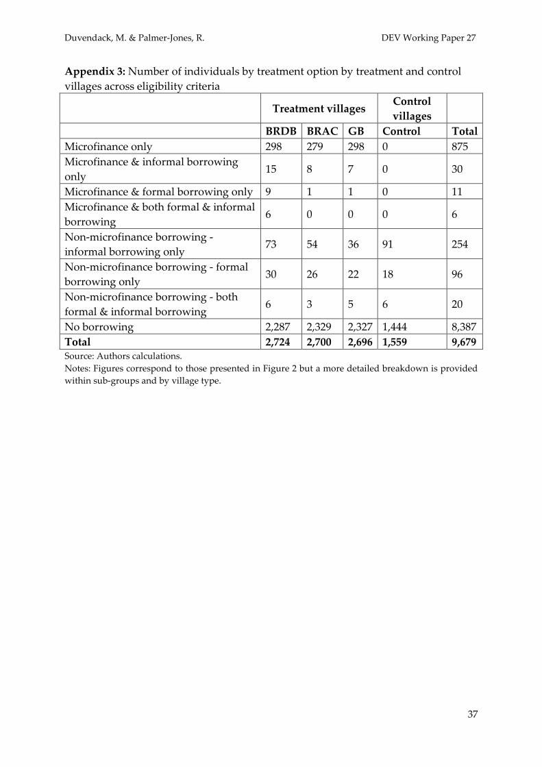
Duvendack, M. & Palmer-Jones, R. DEV Working Paper 27
37
Appendix 3: Number of individuals by treatment option by treatment and control villages across eligibility criteria
Treatment villages Control villages
BRDB BRAC GB Control Total Microfinance only 298 279 298 0 875 Microfinance & informal borrowing only
15 8 7 0 30
Microfinance & formal borrowing only 9 1 1 0 11 Microfinance & both formal & informal borrowing
6 0 0 0 6
Non-microfinance borrowing - informal borrowing only
73 54 36 91 254
Non-microfinance borrowing - formal borrowing only
30 26 22 18 96
Non-microfinance borrowing - both formal & informal borrowing
6 3 5 6 20
No borrowing 2,287 2,329 2,327 1,444 8,387 Total 2,724 2,700 2,696 1,559 9,679 Source: Authors calculations. Notes: Figures correspond to those presented in Figure 2 but a more detailed breakdown is provided within sub-groups and by village type.

Duvendack, M. & Palmer-Jones, R. DEV Working Paper 27
38
Appendix 4: Simple matching estimates across gender using nearest neighbour matching for all four comparison groups with number of matches and pseudo R-squared
Outcome variables
vs
eligible
vs
+
vs
vs
Comparison 1 2 3 4
1-nearest neighbour matching
Variation of log per capita expenditure (Taka)
-0.017* -0.004 0.000 -0.019
Log per capita expenditure (Taka) -0.012 0.003 0.035** -0.081
Log women non-landed assets (Taka)
1.230*** 0.589** 0.115 0.333
Female labour supply, aged 16-59, hours per month
61.70*** 51.92*** 36.92*** 71.62***
Male labour supply, aged 16-59, hours per month
-47.45*** -27.46 32.68** -
259.98***
Girl school enrolment, aged 5-17 years -0.012 0.073* 0.034 0.043
Boy school enrolment, aged 5-17 years
0.006 0.082* 0.053 -0.012
No of treated observations used 861 861 1,275 861
No of untreated observations used 655 674 918 191
Total number of observations 4,123 5,068 5,436 1,229
Pseudo R-squared 0.077 0.130 0.104 0.263

Duvendack, M. & Palmer-Jones, R. DEV Working Paper 27
39
5-nearest neighbour matching
Variation of log per capita expenditure (Taka)
-0.016** -0.004 -0.000 -0.045*
Log per capita expenditure (Taka) -0.014 -0.006 0.024* -0.072*
Log women non-landed assets (Taka)
1.100*** 0.475** 0.389** 0.231
Female labour supply, aged 16-59, hours per month 54.28*** 57.75*** 33.33*** 69.17***
Male labour supply, aged 16-59, hours per month
-27.87* -43.64*** 32.12*** -
254.63***
Girl school enrolment, aged 5-17 years
0.061* 0.073* 0.048* 0.073
Boy school enrolment, aged 5-17 years 0.040 0.082* 0.068** -0.022
No of treated observations used 861 861 1,275 861
No of untreated observations used43 655 674 918 191
Total number of observations 4,123 5,068 5,436 1,229
Pseudo R-squared 0.077 0.130 0.104 0.263
Source: Authors calculations. Notes: *statistically significant at 10%, **statistically significant at 5%, ***statistically significant at 1%. Using PnK data, see footnote 8. Stata routine psmatch2 is applied. The logit model outlined in Table 1 is used. The results in this table refer to the differences in the mean values between matched samples. t-tests before and after matching were employed for all results presented in this table to investigate the differences in the mean values for each covariate X across matched samples; as before, the test provided conclusive results. Standard errors (not reported) are bootstrapped.
43 The identical number of cases of matched untreated for 1- and 5- nearest neighbour matching is further evidence of the lack of plentiful comparison cases.

Duvendack, M. & Palmer-Jones, R. DEV Working Paper 27
40
Appendix 5: Eligibility Criterion Referring to Figure 1, Morduch points out that PnK label any participating households in the programme villages (group D) as eligible, even households that should have been excluded according to the less than 0.5 acres eligibility criterion. As a result, according to Morduch, mistargeting occurred, as Group D contains participants who own more than 0.5 acres of land. Ravallion (2008, p. 3818) and Chemin (p. 465) support Morduch’s view that PnK do not strictly enforce the eligibility criterion. Pitt rationalises this claiming that the value of land of treated households which cultivate/possess more than 0.5 acres is so low that the value of the land of these households is effectively less than the median value of 0.5 acres of average land. If Pitt’s claim is indeed true and the three microfinance programmes do take land quality into account when establishing programme eligibility, then the mistargeted households that participate should have total land values of no more than the median unit value of land of the correctly identified households that participate (that is less than 0.5 acres). The data are depicted in the following Figure. Figure 4: Land unit values by total land value and targeting
Value of 50 Decimals at Median Unit Value of Eligible Participants Land
010
0020
0030
0040
0050
00La
nd U
nit V
alue
(Tak
a)
0 200000 400000 600000 800000Total Value of Land (Taka)
Target Mistargeted
Source: Author’s calculations based on PnK data R1 downloaded from the World Bank website. The median unit value of land of eligible participating households (having less than 0.5 acres of land) equals 1000 Taka per decimal (50 decimals equal 0.5 acres). Thus, one might suggest the cut-off point for establishing programme eligibility is 50,000 Taka, that is mistargeted households that participate should have a total value of

Duvendack, M. & Palmer-Jones, R. DEV Working Paper 27
41
land less than 50,000 Taka. However, 50% of the mistargeted households that participate have total land values of greater or equal to 85,000 Taka, and 72% of those mistargeted households have total land values of greater or equal to 50,000 Taka (a reasonable cut-off for using a value of land criterion). Hence, Pitt’s argument does not convince. Further information and a scatter plot showing the details can be obtained from the authors. PnK support the use of landownership as an eligibility criterion and argue that the virtual absence of an active land market justifies its application (PnK: 970). Morduch provides evidence to the contrary; he argues that there is substantial evidence on an active land market in South Asia (Morduch: 4). He argues that close to one eighth of participants in fact bought substantial amounts of land a few years before the survey was conducted. Chemin and Morduch argue that simply comparing groups E to F or groups E to B (see Figure 1) is misleading due to selection bias. As a result, Morduch proposes comparing the outcomes of groups E + F to those in group B which would provide bias-free impact estimates. However, this comparison assumes that landholdings are exogenous, that is that membership in groups E, F or B is not influenced by self-selection (Morduch: 7). Furthermore, the comparison Morduch proposes does not ‘…reflect general differences across villages’ (Morduch: 8). Therefore, assuming that there are minor spill-over effects from group E to C or A, he suggests employing a simple differences-in-differences (DID) estimation that compares the outcomes of groups E + F to C. Similarly, he recommends conducting a comparison for group A relative to group B (Morduch: 8). After employing these comparisons, Morduch finds no statistically significant impacts of exposure to microfinance. Pitt, and Khandker, 2000, address the potential contamination problem, and, find that it appears to make no substantive difference to the results, and this is supported by our results. To avoid confusion, we report whether we use a de jure or de facto classification.