High Accuracy Nonlinear Control and Estimation for Machine ...

General rights Copyright and moral rights for the publications made accessible in the public portal are retained by the authors and/or other copyright owners and it is a condition of accessing publications that users recognise and abide by the legal requirements associated with these rights.

Users may download and print one copy of any publication from the public portal for the purpose of private study or research.

You may not further distribute the material or use it for any profit-making activity or commercial gain

You may freely distribute the URL identifying the publication in the public portal If you believe that this document breaches copyright please contact us providing details, and we will remove access to the work immediately and investigate your claim.

Downloaded from orbit.dtu.dk on: Aug 25, 2022

High Accuracy Nonlinear Control and Estimation for Machine Tool Systems

Papageorgiou, Dimitrios

Publication date:2017

Document VersionPublisher's PDF, also known as Version of record

Link back to DTU Orbit

Citation (APA):Papageorgiou, D. (2017). High Accuracy Nonlinear Control and Estimation for Machine Tool Systems. TechnicalUniversity of Denmark, Department of Electrical Engineering.

https://orbit.dtu.dk/en/publications/7b33f140-c7cd-4395-a148-c2438cf1f13c

Dimitrios Papageorgiou

High Accuracy Nonlinear Controland Estimation for Machine ToolSystems

PhD Thesis, August 2017

High Accuracy Nonlinear Controland Estimation for Machine Tool

Systems


Technical University of DenmarkKgs. Lyngby, Denmark, 2017

Technical University of DenmarkAutomation and Control (AUT)Elektrovej Building 326DK-2800, Kgs. LyngbyDenmarkPhone: (+45) 45 25 35 73Email: [email protected]

mailto:[email protected]

www.elektro.dtu.dk

Summary

Component mass production has been the backbone of industry since the second

industrial revolution, and machine tools are producing parts of widely varying

size and design complexity. The ever-increasing level of automation in modern

manufacturing processes necessitates the use of more sophisticated machine tool

systems that are adaptable to different workspace conditions, while at the same

time being able to maintain very narrow workpiece tolerances. The main topic of

this thesis is to suggest control methods that can maintain required manufacturing

tolerances, despite moderate wear and tear. The purpose is to ensure that full

accuracy is maintained between service intervals and to advice when overhaul is

needed.

The thesis argues that quality of manufactured components is directly related

to the positioning accuracy of the machine tool axes, and it shows which low

level control architectures are used to position the machining tool relatively to the

material being processed. While existing algorithms provide sufficient accuracy after

commissioning of the machine by experts, the thesis shows how they fall short in

keeping required tolerances in the presence of equipment wear, unless they are

re-tuned by experts.

The goal of this research has therefore been investigation and development of

advanced control and estimation algorithms, which facilitate high-accuracy machine-

tool axis positioning, and are robust to equipment degradation and wear.

This thesis presents the findings of the research conducted during the three years

of the PhD program at the Technical University of Denmark. The research has been

carried out in close collaboration with Siemens AG in Nuremberg, who sponsored

the research. Siemens also provided state-of-the-art industrial equipment to facilitate

experimental testing and validation. DTU added mechanical components to test the

development of friction and backlash. The scientific-technical contributions of the

research fall into three parts, which also constitute the structure of the thesis.

The first part concerns the development of an efficient description of a generic

machine-tool axis system. A detailed mathematical model is derived that captures

the most important axis dynamics. Positioning degrading phenomena, such as

ii

friction and backlash, are expressed as nonlinear axis torques. Identification of the

test rig parameters and sensitivity analysis is carried out, to highlight the significance

of individual model parameters.

The second contribution of this research pertains to the investigation of different

nonlinear control strategies and architectures for the positioning of the axis. Eight

position controllers based on sliding-mode and adaptive principles are designed,

implemented and tested on the experimental setup. A set of quantitative and

qualitative criteria is used for the systematic comparison of the methods. The

evaluation results show that four out of the eight designs provide superior positioning

accuracy and resilience to unknown and varying friction, in comparison to the state-

of-the-art proportional-integral control solutions.

The third part of the research relates to the development of online backlash

estimation algorithms for machine-tools. The proposed method utilizes position and

velocity measurements in a cascaded scheme consisting of a sliding-mode velocity

observer and an adaptive deadzone angle estimator. A series of experiments is

conducted for testing the algorithm in various operation scenarios under different

levels of uncertainty. The results show that the estimator identifies the unknown de-

adzone angle and changes in it with sufficient accuracy and can, therefore, facilitate

backlash compensation, as well as equipment wear assessment and prognosis.

The scientific results of this research have been summarized in three journal

articles, which have been submitted, and an article presented at the IFAC World

Congress 2017 that has been published.

Resumé

Masseproduktion af komponenter har været en hjørnesten i industrien siden

den anden industrielle revolution med maskiner der fremstiller emner af meget

varierende størrelse og kompleksitet. Med automatiseret fremstilling af stadig mere

divercificerede og komplekse emner er der både behov for at kunne tilpasse styringen

af en maskine til nye emner og for at opretholde høje krav til fremstillingstoleran-

cer. Kravet om præcision gælder både når en maskine er helt ny og over tid, når

maskindele påvirkes af slidtage.

Hovedemnet for dette forskningsarbejde er at anvise styrings- og reguleringsmeto-

der, som kan sikre at en høj fremstillingsnøjagtighed opretholdes, uanset begyndende

mekanisk slidtage. Hensigten er at sikre, at der arbejdes med fuld præcision imellem

serviceeftersyn, samt at kunne anvise hvornår næste vedligehold bliver nødvendigt.

Afhandlingen tager udgangspunkt i at tolerancer i maskinel bearbejdning hænger

direkte sammen med nøjagtigheden hvormed et skærende værktøj kan positioneres

i forhold til det emne der bearbejdes. Når en maskine er ny, og dens nummeriske

styring er indjusteret, har den fuldt tilfredsstillende præcision.

Afhandlingen viser at eksisterende styringer mister præcision, når slidtage indfin-

der sig, med mindre regulatorparametre gen-justeres af eksperter. Formålet med

forskningsarbejdet har derfor været at undersøge og foreslå avancerede metoder

til styring og estimering, som kan tilbyde højpræcisions styring der ikke er følsom

overfor mekanisk slidtage.

Afhandlingen præsenterer resultaterne af et tre-årigt phd program på Danmarks

Tekniske Universitet. Forskningen er foregået i samarbejde med Siemens AG, Nürn-

berg, som har sponsoreret projektet og også har stillet state-of-art udstyr til rådighed

for laboratorietest og validering.

Afhandlingen er opdelt i tre dele med hver deres teknisk-videnskabelige bidrag.

I første del udarbejdes en generel matematisk beskrivelse af en enkelt akse i en

fremstillingsmaskine. Modellen omfatter den nødvendige dynamik og inkluderer

slidtage, i form af friktion og slør, som ikkelineære elementer i modellen. Parametre

i modellen fastlægges teoretisk og eksperimentelt, bl.a. med anvendelse af system

identifikation. De enkelte parametres betydning vurderes udfra den virkning på

iv

præcision der kan iagtages, når de ændres.

I anden del undersøges udvalgte ikkelineære reguleringsmetoder, der er baseret

på sliding mode og adaptive principper. Afhandlingen beskriver hvordan arkitektur

og parametre bestemmes for de valgte metoder. Konvergens bevises teoretisk, hvor

det er relevant, og afhandlingen vurderer styringskvalitet i form af resultater fra

simuleringer og fra eksperimenter i laboratoriet. Reguleringsmetodernes kvalitet

vurderes samlet udfra et sæt af indikatorer, der udtrykker reguleringskvalitet på

en måde som er relevant for den industrielle anvendelse. Resultaterne viser at fire

af otte ikkelineære styringsalgoritmer opnår bedre præcision og robusthed overfor

ukendt og langsomt øget friktion end den eksisterende konventionelle regulering.

I tredie del undersøges hvordan mekanisk slør kan estimeres for en nummerisk

styret maskine medens den udfører normal produktion. Der foreslås en ny metode

til estimering af slør. Den anvender en kombination af en sliding mode observer

og en adaptiv estimator til at at opnå en høj følsomhed. Estimationsalgoritmen er

valideret under forskellige realistiske servo bevægelser, og for forskellige niveauer af

mekanisk slør. Den eksperimentelle validering viser at den nye algoritme vil kunne

anvendes både til kompensering af slør og til prognose af hvornår vedligehold skal

foretages.

De videnskabelige resultater af dette arbejde er sammenfattet i tre tidsskrifts-

artikler, som er indsendt, og i en artikel til IFAC World Congress i 2017, som er

publiceret.

Preface

This project was prepared as a collaboration between the Automation and Control

group in the Department of Electrical Engineering of the Technical University of

Denmark (DTU) and Siemens AG in the context of the DTU PhD program. The

industrial partner was the exclusive sponsor of the project.

The project advisors were:

• Professor Mogens Blanke (principal supervisor), Department of Electrical

Engineering, Automation and Control group, DTU.

• Associate professor Hans Henrik Niemann (co-supervisor), Department of

Electrical Engineering, Automation and Control group, DTU.

• Dr.-Ing. Jan H. Richter (company supervisor), Digital Factory Division, Techno-

logy and Innovations, Siemens AG.

This thesis consists of a summary report of all research findings gathered as a

collection of submitted articles in peer reviewed scientific journals and published in

conference proceedings in the period 2014-2017.

Kongens Lyngby, August 2017


List of Publications

Publications included in the thesis

(A) D. Papageorgiou, M. Blanke, H. H. Niemann, and J. H. Richter. “Friction resi-

lience of machine tool controls - Classic, sliding mode and nonlinear adaptive

techniques compared”. Control Engineering Practice (2017). : Submitted paper

under review.

(B) D. Papageorgiou, M. Blanke, H. H. Niemann, and J. H. Richter. “Friction-

resilient position control for machine tools - Adaptive and sliding-mode met-

hods compared”. Control Engineering Practice (2017). : Submitted paper under

review.

(C) D. Papageorgiou, M. Blanke, H. H. Niemann, and J. H. Richter. “Robust

backlash estimation for industrial drive-train systems - theory and validation”.

Transactions on Control Systems Technology (2017). : Submitted paper under

review.

(D) D. Papageorgiou, M. Blanke, H. H. Niemann, and J. H. Richter. “Backlash

estimation for industrial drive-train systems” (July 2017). : To appear in

IFAC-PapersOnLine.

Publications not included in the thesis

(E) D. Papageorgiou, M. Blanke, H. H. Niemann, and J. H. Richter. “Fault tole-

rance for industrial actuators in absence of accurate models and hardware

redundancy”. 2015 IEEE Conference on Control Applications (CCA). Sept. 2015,

pp. 1887–1894. DOI: 10.1109/CCA.2015.7320885.

https://doi.org/10.1109/CCA.2015.7320885

Acknowledgments

"Πᾶσα τὲ ἐπιστήμη χωριζομένη δικαιοσύνης καὶ τῆς ἂλλης

ἀρετής πανουργία οὐ σοφία φαίνεται."

Every science departing from justice and other virtue reveals

cunningness and not wisdom.

— Plato, Menexenus 247a

During my PhD studies I enjoyed the privilege of having three charismatic

researchers and accomplished professionals as supervisors. Professor Mogens Blanke

has been my main advisor and academic mentor. Conducting research under his

wing made it possible for small ideas to transform into high-quality results. His

continuous guidance and support, irrespectively of the clock index position, have

been catalytic in my development as a researcher, for which I am deeply grateful. I

would like to thank my co-supervisor Associate Professor Hans-Henrik Niemann, for

always being available for questions and for advising me on topics on classic control,

frequency domain analysis and system identification. During the entire project, my

advisor from Siemens Dr. Jan H. Richter had been sharing his expertise in control

design and planning. Through his meticulous and dedicated supervision he taught

me how to project academic research ideas onto real industrial applications. I take

the chance here to thank my supervisors, as well as the general manager of the

project Dr. Jörg Neidig, for believing in me and providing me with the opportunity

of working on such an exciting research project.

During the second year of my project I had a short stay at Siemens AG facilities in

Nuremberg, where I presented my research ideas and received training on Siemens

drives commissioning. I would like to thank the Siemens team from the Digital

Factory division for their valuable comments, as well as the interesting discussions

on the project. Special thanks to Siemens motion control experts Dr. Hans-Georg

Koepkin and Dr. Carsten Hamm, who shared their knowledge and experience with

me, regarding several technical topics in modelling and control. It was Dr. Hamm’s

tireless efforts and expertise that made the integration of my control designs into

the test rig possible.

x

Many times during my project did I knock on Associate Prof. Roberto Galeazzi’s

office door for a "five-minute" question and I always came out of his office with

answers and good ideas. For that I full-heartedly thank him. I would also like to

thank Dr. Konstantinos Poulios, Kristian Sloth Lauszus and Dr. Moises Pacheho for

their help in designing and manufacturing the various extensions for the project’s

experimental setup.

Working at the Automation and Control Group in DTU has been truly inspiring.

During these past three years I have had the pleasure of cooperating and socializing

with people of excellent quality, whose company I cherish. I especially want to

thank my treasured friends Mikkel Cornelius Nielsen, Dr. Remus Michail Prunescu,

Nicholas Peter Hansen and Leon Nagel for all these "science-plus-coffee" sessions,

where we all used to share our thoughts and ideas on our projects. I would also like

to thank Dr. Andreas Søndergaard Pedersen, André Krabdrup Sekunda, Emil Krabbe

Nielsen, Robert Miklos and the rest fellow-researchers from the AUT group.

My trajectory during my PhD studies would have been much less smooth had

I not had the endless support of my two closest friends Konsantinos Goulas and

Alexandros Meletis, for which I am deeply grateful. I would also like to thank

my friend and teacher Dimitrios Metzikof Papadakis for his guidance and all the

philosophical discussions we had on science ethics and virtue.

Finally, I would like to express my utmost gratitude to my father Epameinondas,

mother Sotiria, sister Kalomoira and uncle Evaggelos for their love and support

during all these years. Their moral paedeia has constantly been an example to me

for pursuing a life of virtue. I thank them, as well as my grandparents and the rest

of my family for always believing in me.

Table of Contents

Summary i

Resumé iii

Preface v

List of Publications vii

Acknowledgments ix

List of Abbreviations xv

Notation convention xix

1 Introduction 1

1.1 Background . . . . . . . . . . . . . . . . . . . . . . . . . . . . . . . . 1

1.2 Motivation, Goals and Scope of the Project . . . . . . . . . . . . . . . 4

1.3 Thesis Outline . . . . . . . . . . . . . . . . . . . . . . . . . . . . . . . 6

2 State Of The Art 7

2.1 Machine Tool Position Control . . . . . . . . . . . . . . . . . . . . . . 7

2.2 Friction Modelling and Compensation . . . . . . . . . . . . . . . . . 8

2.3 Backlash Modelling and Estimation . . . . . . . . . . . . . . . . . . . 9

2.4 Sliding-Mode Controllers and Observers . . . . . . . . . . . . . . . . 11

2.5 Adaptive control . . . . . . . . . . . . . . . . . . . . . . . . . . . . . 12

3 Summary of Main Contributions 15

4 System Modelling 19

4.1 Introduction . . . . . . . . . . . . . . . . . . . . . . . . . . . . . . . . 19

4.2 System Description . . . . . . . . . . . . . . . . . . . . . . . . . . . . 19

4.3 Mathematical Model . . . . . . . . . . . . . . . . . . . . . . . . . . . 25

xii Table of Contents

4.4 Parameter Sensitivity Analysis and Identification . . . . . . . . . . . . 32

4.5 Conclusions . . . . . . . . . . . . . . . . . . . . . . . . . . . . . . . . 48

5 Advanced Friction-Resilient Axis Positioning Control 51

5.1 Introduction . . . . . . . . . . . . . . . . . . . . . . . . . . . . . . . . 51

5.2 Sliding-Mode and Adaptive Methodologies . . . . . . . . . . . . . . . 52

5.3 Controller Design . . . . . . . . . . . . . . . . . . . . . . . . . . . . . 56

5.4 Controllers Evaluation . . . . . . . . . . . . . . . . . . . . . . . . . . 70

5.5 Additional Control Designs . . . . . . . . . . . . . . . . . . . . . . . . 85

5.6 Conclusions . . . . . . . . . . . . . . . . . . . . . . . . . . . . . . . . 94

6 Backlash Estimation 97

6.1 Introduction . . . . . . . . . . . . . . . . . . . . . . . . . . . . . . . . 97

6.2 Backlash Modelling and Problem Formulation . . . . . . . . . . . . . 97

6.3 Deadzone Angle Estimation . . . . . . . . . . . . . . . . . . . . . . . 100

6.4 Simulation and Experimental Results . . . . . . . . . . . . . . . . . . 104

6.5 Conclusions . . . . . . . . . . . . . . . . . . . . . . . . . . . . . . . . 109

7 Conclusions and Future Research 113

7.1 Summary of Conclusions . . . . . . . . . . . . . . . . . . . . . . . . . 113

7.2 Future Research . . . . . . . . . . . . . . . . . . . . . . . . . . . . . . 114

Paper A Friction Resilience of Machine Tool Controls - Classic, Sliding-

Mode and Nonlinear Adaptive Techniques Compared 117

A.1 Introduction . . . . . . . . . . . . . . . . . . . . . . . . . . . . . . . . 118

A.2 System Description and Problem Formulation . . . . . . . . . . . . . 120

A.3 Mathematical Model . . . . . . . . . . . . . . . . . . . . . . . . . . . 122

A.4 Tool Position Control Methods . . . . . . . . . . . . . . . . . . . . . . 126

A.5 Experiments and Evaluation . . . . . . . . . . . . . . . . . . . . . . . 137

A.6 Conclusions and Future Work . . . . . . . . . . . . . . . . . . . . . . 150

Paper B Friction-Resilient Position Control for Machine Tools - Adaptive

and Sliding-Mode Methods Compared 155

B.1 Introduction . . . . . . . . . . . . . . . . . . . . . . . . . . . . . . . . 156

B.2 System Description and Problem Formulation . . . . . . . . . . . . . 157

B.3 Mathematical Model . . . . . . . . . . . . . . . . . . . . . . . . . . . 159

B.4 Tool Position Control Methods . . . . . . . . . . . . . . . . . . . . . . 161

B.5 Experiments and Evaluation . . . . . . . . . . . . . . . . . . . . . . . 174

B.6 Discussion . . . . . . . . . . . . . . . . . . . . . . . . . . . . . . . . . 184

B.7 Conclusions and Future Work . . . . . . . . . . . . . . . . . . . . . . 189

Table of Contents xiii

Paper C Robust Backlash Estimation for Industrial Drive-Train Systems -

Theory and Validation 191

C.1 Introduction . . . . . . . . . . . . . . . . . . . . . . . . . . . . . . . . 192

C.2 System Description and Problem Formulation . . . . . . . . . . . . . 193

C.3 Backlash Deadzone Angle Estimation . . . . . . . . . . . . . . . . . . 198

C.4 Robustness Analysis . . . . . . . . . . . . . . . . . . . . . . . . . . . 206

C.5 Simulation Results . . . . . . . . . . . . . . . . . . . . . . . . . . . . 209

C.6 Experimental Results . . . . . . . . . . . . . . . . . . . . . . . . . . . 211

C.7 Conclusions . . . . . . . . . . . . . . . . . . . . . . . . . . . . . . . . 219

Paper D Backlash Estimation for Industrial Drive-Train Systems 221

D.1 Introduction . . . . . . . . . . . . . . . . . . . . . . . . . . . . . . . . 222

D.2 System Description and Problem Formulation . . . . . . . . . . . . . 223

D.3 Backlash Deadzone Angle Estimation . . . . . . . . . . . . . . . . . . 227

D.4 Simulation Results . . . . . . . . . . . . . . . . . . . . . . . . . . . . 231

D.5 Conclusions . . . . . . . . . . . . . . . . . . . . . . . . . . . . . . . . 233

Appendix Supplementary Material 235

I The dq0 Transformation . . . . . . . . . . . . . . . . . . . . . . . . . 235

II Basic Definitions . . . . . . . . . . . . . . . . . . . . . . . . . . . . . 235

III Elements of Lyapunov Stability Theory . . . . . . . . . . . . . . . . . 237

IV Proof of ISS Property of eθ (I&I-AC) . . . . . . . . . . . . . . . . . . . 239

V Proof of ISS Property of eθ (ABSC) . . . . . . . . . . . . . . . . . . . 240

VI Proof of BIBO Stability of χ With Respect to ωm (SFL1) . . . . . . . . 240

VII Calculation of a (ABSC) . . . . . . . . . . . . . . . . . . . . . . . . . 241

VIII Taylor Expansion Theorem . . . . . . . . . . . . . . . . . . . . . . . . 243

IX Proof of Property (C.34) . . . . . . . . . . . . . . . . . . . . . . . . . 243

Bibliography 245

List of Abbreviations

L1AC L1 Adaptive Control. 13, 14

ABSC Adaptive Backstepping Controller. 12, 14, 63, 65, 66, 69, 72, 74, 72, 79, 80,

113, 156, 164, 174, 176, 178, 179, 181, 182, 183, 185, 182, 185

ACC Adaptive Control with Constraints. 118

ACO Adaptive Control with Optimization. 118

ASTSMC Adaptive Super-Twisting Sliding-Mode Controller. 68, 69, 74, 72, 74, 77,

80, 156, 170, 172, 174, 176, 178, 180, 181, 182, 183, 185, 182

BIBO Bounded Input-Bounded Output. 89, 241

CAM Computer Aided Manufacturing. 3

CCC Cross-Coupling Control. 7, 118

CI Complexity Index. 72

CIT Circular Interpolation Test. 72, 142, 176

CNC Computerized Numerical Control. 1, 3, 4, 192, 222

CP Control Power. 70, 141, 176

CU control unit. 22

ECP Error-Control Power product. 70, 141, 144, 149, 145, 149, 176, 181, 182

EKF Extended Kalman Filter. 10, 192, 222

ES Exponentially Stable. 67, 171

GAC Geometry Adaptive Control. 118

xvi List of Abbreviations

I&I-AC Immersion and Invariance Adaptive Control. 13, 14, 61, 62, 66, 69, 72, 74,

72, 79, 80, 113, 129, 133, 137, 140, 143, 144, 145, 147, 149, 151, 145, 185

IAC Individual Axis Control. 7, 8

ISE Integral Square Error. 70, 140, 176

ISS Input-to-State Stable. 137, 169, 204, 205, 208, 239, 240, 241

ITSE Integral Timed Square Error. 70, 141, 176

LMI Linear Matrix Inequality. 59, 128

LTI Linear Time-Invariant. 171, 172

MAE Maximum Absolute Error. 72, 70, 72, 74, 72, 74, 80, 86, 92, 140, 143, 144,

145, 149, 150, 149, 176, 178, 179, 181, 182, 181, 184, 182, 184, 189

MAEE Maximum Absolute Estimation Error. 106, 107, 109, 212, 214, 215

MAPE Maximum Absolute Phase Error. 70, 72, 70, 74, 141, 142, 145, 176, 181,

182

MRAC Model Reference Adaptive Control. 12, 13, 55, 128

NAC Nonlinear Adaptive Control. 12, 14, 59, 60, 61, 63, 66, 69, 72, 74, 72, 79, 80,

113, 128, 129, 130, 133, 135, 136, 137, 140, 143, 144, 145, 147, 149, 151,

145, 185

NCSTSMC Nested Continuous Singular Terminal Sliding-Mode Controller. 85, 86

OSTSMC Output Super-Twisting Sliding-Mode Controller. 66, 68, 69, 74, 72, 74,

77, 80, 156, 170, 172, 173, 174, 176, 178, 180, 181, 182, 183, 185, 182

P Proportional. 4, 5, 7, 8, 15, 16, 51, 56, 58, 69, 72, 74, 72, 74, 77, 80, 86, 87, 90,

92, 94, 113, 117, 118, 119, 124, 127, 128, 129, 130, 139, 140, 149, 150, 155,

156, 161, 162, 176, 178, 183, 184, 182, 189, 193

PDE Partial Differential Equation. 147

PDEs Partial Differential Equations. 61

PE Persistence of Excitation. 206, 230, 236

List of Abbreviations xvii

PI Proportional-Integral. 4, 5, 7, 8, 15, 16, 29, 51, 54, 55, 56, 57, 72, 74, 72, 74,

80, 86, 92, 94, 104, 113, 117, 118, 119, 124, 137, 139, 140, 143, 144, 145,

147, 149, 150, 145, 155, 156, 161, 176, 178, 179, 182, 183, 185, 182, 189,

193, 231

PID Proportional-Integral-Differential. 7

PMSM permanent magnet synchronous motor. 20, 22, 23, 25, 29, 120, 127, 129,

164, 193

PMSMs permanent magnet synchronous motors. 157, 174, 235

SFL1 State-Feedback L1 adaptive controller. 85, 87, 92

SMC Sliding-Mode Control. 8, 11, 12, 53, 54, 58, 63, 72, 74, 77, 85, 119, 127, 151,

156, 169

SMO Sliding-Mode Observer. 11, 12, 102, 199, 200, 212, 215, 219, 228, 229

STSMC Super-Twisting Sliding-Mode Controller. 11, 12, 58, 59, 66, 67, 69, 72, 74,

72, 74, 77, 80, 113, 127, 128, 137, 140, 143, 144, 145, 147, 150, 151, 145,

169, 170, 172, 184, 185, 189

STSMO Super-Twisting Sliding-Mode Observer. 102, 103, 105, 109, 114, 199, 205,

206, 208, 209, 212, 222, 228, 230, 231, 233

UB Uniformly Bounded. 204

UGAS Uniformly Globally Asymptotically Stable. 103, 137, 169, 201, 202, 205, 207,

219

UGB Uniformly Globally Bounded. 103, 208, 209, 219

ULES Uniformly Locally Exponentially Stable. 103, 202, 204, 205, 206

Notation Convention

The following notation convention applies to the entire thesis report:

Table 1: Notation convention.

Notation rule Explanation Example

Lower/Upper-case normal font Scalar variable, function or constant δ,ΣLower-case bold font Vector variable or function ϑ,φ1(x)Upper-case bold font Matrix A

Upper-case calligraphic font Set MSingle-bar brackets Norm of scalar or matrix |ωr|L∞ , |B|Double-bar brackets Norm of vector ‖x‖"hat" symbol Estimate of variable δ

"tilde" symbol Estimation error δ

"dot" symbol Time-derivative of variable ϑ

diag(·) Diagonal of square matrix diag(Γ)Dimension superscript Set of n×m real matrices Γ ∈ R2×2

>0

Cn Set of n−times differentiable functions C3

f (n) nth time derivative of f(t) θ(3)r

Chapter 1

Introduction

1.1 Background

Automated manufacturing is one of the pillars of modern industry. From aero-

space and auto-mobile applications to medical equipment and small-scale electronic

devices, the ability for fast mass production of a wide range of components has

fuelled the technological advances, boosting the global economy during the past

decades. According to the World Bank Database [6] manufacturing constitutes

approximately 54% of the global industrial economy, while the value-added during

2014 was $12.165 trillion, which amounts to 14.9% of the world GDP in that year.

Figure 1.1 shows the increase of the value-added in manufacturing industries during

the period 2000-2014.

The advances in Computerized Numerical Control (CNC) in machine-tool systems

within the last decades have facilitated the increase of the automation level in

manufacturing, allowing faster and larger production of various components for

nearly all industrial applications. The increasing demand for faster prototyping and

product development [7] has also led to more sophisticated machine tool designs

that allow for uninterrupted workpiece processing at smaller times.

Modern CNC machine tools vary in size, number of axes and tools, depending

on the application and the tasks they are used for (e.g. milling, boring, grinding,

turning, plasma cutting). The processing of the workpieces takes place in a secured

cabinet, next to which there is an operating panel (see Figure 1.2). The basic parts of

a machine tool include the spindle, which is the main rotary axis of the machine, the

table, i.e. the platform where the workpiece is placed, several moving axes and the

tool. Fully automated machine tools have an integrated tool-exchanging mechanism

and a collection of different processing tools that add task flexibility to the machine.

All the moving parts of the machine, i.e. the spindle, the axes and the table, are

2 Chapter 1. Introduction

2000 2005 2010 2014

0

5

10

15

Year

Valu

e-ad

ded

inU

S$tr

illio

n

2000 2005 2010 2014

0

1

2

3

Year

China GermanyJapan USA

Figure 1.1: Manufacturing, value added for world economy (left) and for the industrial

"leading" countries (right) in US$ trillion. The data was taken from the World Bank Database

[6].

Figure 1.2: (Left): Interior of a machining cabinet with operating panel. (Right): Machine

tool with three linear axes. Sources: [8, 9].

1.1. Background 3

actuated by electrical drives, each of which has a dedicated control system. The

combination of all the motions results in a predefined configuration between the

processing tool and the workpiece that is machined. The quality of the manufactured

component, reflected in the correct dimensioning, surface finishing and consistency

to the component design, is directly related to the accurate tool-workpiece relative

positioning during the entire process.

The ever-increasing complexity of mechanical designs requires high-accuracy tool

positioning in machine-tool systems at the order of 10µm or lower [10]. Achieving

such tolerances assumes not only the availability of high-resolution measuring

equipment but also the detailed and fine tuning of all the procedures in each stage

of the machining. A typical automated manufacturing process consists of three basic

levels [11] (see also Figure 1.3):

• CNC programming: With the mechanical design of the component as input

the Computer Aided Manufacturing (CAM) software produces a sequence

of motion directives for the axes of the machine tool, through which the

machining of the workpiece can be made.

• Trajectory generation: The CAM translator feeds the program to an inter-

polator, which takes the machine characteristics (e.g. tool dimensions and

geometry, spindle feed rate etc.) as input. Typically, machine tools are over-

dimensioned, such that deformations during machining have little influence

on the product quality [8]. The interpolator generates position setpoints for

each axis of the machine.

• Axis control: A closed-loop control system ensures that each axis is positioned

according to the setpoints commanded by the trajectory generator.

CAM softwareMechanical

design

CAM translator/

InterpolatorMachine

characteristics

Axes position controlPosition setpoints

Axes dynamics

Measuring devices

Axe

spo

siti

ons

Position closed-loop SystemCNC Programming

Trajectory generator

Figure 1.3: Automated component manufacturing chain.


Workpiece tolerances can be compromised by a number of different machining

errors. Such errors can be related to the geometry of the machine and the tool (mi-

salignment of the machine parts or the workpiece, tool deflection and wear, thermal

expansion, etc.) or to measuring faults (e.g. uncertainty of the reference position,

different measured position during reversal of motion) [11]. Although these errors

are usually compensated for by recalibration of the machine and trajectory path

correction, additional mechanical phenomena, such as variable friction, backlash

and changing load inertias, show up during workpiece processing. These pheno-

mena further complicate the machining process and will compromise the workpiece

tolerances, unless properly handled by closed-loop control algorithms. Consequently,

the most significant contribution to maintain workpiece tolerances, comes from the

low-level axis control, the lowest process layer.

1.2 Motivation, Goals and Scope of the Project

High-accuracy relative positioning between tool and workpiece is essential for

ensuring proper manufacturing of machined components. Counteracting complex

accuracy-degrading phenomena in CNC machine tools, such as friction and backlash,

necessitates the use of appropriate compensating algorithms at the level of axis posi-

tion control. These closed-loop strategies can ensure confinement of the positioning

errors within the tolerances only when the degrading phenomena are accurately

described. In cases of varying friction and load parameters, or developing deadzones

due to wear, conventional axis position controllers - typically based on Proportio-

nal (P) and Proportional-Integral (PI) principles - often fail to keep the workpiece

tolerances. This compromises the quality of the end product. To compensate for

this loss of positioning accuracy the axes’ closed-loop control parameters have to be

retuned to match the new degrading phenomena each time quality loss is observed.

This inevitably leads to increased maintenance cost and, therefore, decrease of the

overall efficiency of a production line.

In the light of the emerging Industrie 4.0 [12], future fully-automated CNC

machine tools that can adapt [13] to varying workspace conditions, and are robust

to equipment wear, may facilitate a wide penetration in the manufacturing market,

offering larger competitive advantage. As a direct consequence of this, current

axis-positioning solutions will have to be modified or completely redesigned such

that they include the desirable robustness and adaptability features. This motivates

the investigation of low-level control strategies taken from the arsenal of advanced

nonlinear control theory. As outlined, focus should be on their applicability to the

positioning problem in machine tools, as well as to robustness and adaptive features.

1.2. Motivation, Goals and Scope of the Project 5

An additional aspect of the future self-healing manufacturing systems relates to

wear assessment and prognosis. Estimating unknown or varying parameters that

fully describe degrading phenomena not only may enhance error-compensation

mechanisms in the position control loops, but could also be used to assess equip-

ment degradation and provide prognosis of component lifetime. Such feature, by

extension, would facilitate more efficient maintenance scheduling.

To this end, the current research project, fully funded by SIEMENS AG, and in

the context of the PhD program at the Technical University of Denmark, focuses

on developing advanced control and estimation strategies for robust, high-accuracy

positioning in machine tools. The goals of the project were defined as follows:

1. To investigate the possibilities of employing nonlinear control strategies that

provide high-accuracy positioning in machine tool systems in the presence of

wear.

2. To establish an experimental setup with state-of-the-art industrial equipment,

on which the developed methods can be tested. The physical hardware should

facilitate validation of the theoretical findings and highlight design and appli-

cability challenges of the methods.

3. To research estimation methods that can be used in machine tool control

loops for compensating various degrading phenomena and for equipment wear

assessment.

Based on these general goals, the project scope includes:

• Derivation of an appropriately detailed mathematical model of a single-axis

drive train, to be used as the test bench for evaluation of high-accuracy control

methods. The drive-train system serves as an abstraction of a single axis

in a real machine-tool. Critical degrading phenomena, namely friction and

backlash, should be effectively described and integrated into the drive-train

model.

• Design, implementation and testing of various nonlinear control strategies for

high-accuracy positioning in machine tools.

• Systematic comparison of the derived methods’ accuracy and robustness fea-

tures to those of the conventional P-PI solutions. The controllers should be

evaluated with respect to their friction resilience by employing quantitative

and qualitative performance criteria, similar to the evaluation methods used

in the industry.


• Development of an algorithm for online accurate estimation of deadzones

occurring in coupling components between the different mechanical parts of

a drive train. This estimation scheme could be used to describe developing

backlash, and the size of the deadzone could facilitate more effective backlash

compensation in the control loops. Additionally, it could serve as a means of

assessing wear in the coupling equipment.

1.3 Thesis Outline

The structure of the thesis follows the scheme of a collection of articles, where

main results are submitted to journals and per-reviewed conferences in the course

of study. The main body of the dissertation offers a comprehensive summary of the

results obtained throughout the entire project, while technical details are analytically

given in the appended articles. The only exception is Chapter 4, the results in which

were not included in any of the listed publications.

After the introductory Chapter 1, the thesis continues with the presentation of

state-of-the-art methods in control and backlash estimation for machine-tools, given

in Chapter 2. Chapter 3 lists the main contributions of this research.

The detailed derivation of a drive-train mathematical model and the test rig are

presented in Chapter 4. The relevance of the model to the experimental system

and to the real machine tool axes is discussed along with the considered modelling

assumptions. Sensitivity analysis and estimation of system unknown parameters are

also presented.

Chapter 5 discusses the detailed design, implementation and performance of six

nonlinear position control methods based on sliding-mode and adaptive principles.

The experimental results are interpreted and juxtaposed to the specific assumption

made for each method. An overall ranking of the controllers is provided. Two

additional designs that did not meet the performance requirements are discussed

and reasons to their lack of performance are addressed.

Online estimation of the deadzone angle between the two parts of the drive train

is presented in Chapter 6. A new model of the backlash phenomenon is first sugge-

sted. It is based on a varying shaft stiffness approach to overcome mathematical

requirements to smoothness of nonlinearities when applying certain nonlinear design

methods. The design of the deadzone estimator is presented next, followed by a dis-

cussion on the robustness of the method against model and parameter uncertainties.

The performance of the estimation scheme is assessed through experiments.

Finally, Chapter 7 gives a retrospective evaluation of the findings in the entire

project along with directions on future research possibilities.

Chapter 2

State Of The Art

This chapter provides a summary of the most fundamental and recent advances

on the theories and methodologies used in this project. The review starts with

a report of the conventional machine tool control techniques and continues with

results on friction description and compensation. The modelling and estimation

of backlash in mechanical systems are discussed next. The last two sections of the

chapter give a general overview of nonlinear control and estimation methods that

are later employed in this project.

2.1 Machine Tool Position Control

Detailed presentation of different machine tool-positioning strategies was pro-

vided in [14]. State-of-the-art positioning solutions follow two main approaches.

The first one is referred to as Cross-Coupling Control (CCC) [15], where the control

loops of all machine’s axes are considered simultaneously, and the control objective

is expressed as a contour-error regulation problem [16, 17]. In the second approach,

called Individual Axis Control (IAC), each axis is handled separately. The effects of

dynamics of other axes are treated as disturbances, and the control design reduces to

that of individual axes [18]. Results in high-accuracy machine tool position control

from both these categories use P-PI control loops and assume accurate knowledge of

the system parameters.

Several methods that employ adaptation schemes have been used to address

parameter uncertainty in machine tool systems. These control strategies rely on

adjusting either the machine operating parameters (feed rate, spindle speed etc.)

[19] or the tool geometry [20], such that the contouring error is sufficiently small

and certain constraints (eg. regarding cutting forces) are satisfied. Online optimi-

zation has also been used to account for vibrations during cutting and tool wear

8 Chapter 2. State Of The Art

[21]. Apart from few exceptions (see [22] for a varying-gain Proportional-Integral-

Differential (PID) machine tool controller and [23] for adaptive CCC that accounts

for unknown inertial matrix), the majority of machine-tool adaptive techniques do

not utilize parameter estimation in the system dynamics. Such feature could provide

information of the wear level in the machine equipment. This could be achieved

through the use of nonlinear and adaptive control algorithms in IAC architectures,

because the problem of nonlinear position control for flexible axes is well explored.

Indeed, a number of relevant studies that employ techniques from nonlinear

control theory, such as the Sliding-Mode Control (SMC) and the nonlinear Adaptive

Control, have been reported in the literature regarding axis positioning. A gene-

ral framework for nonlinear adaptive control for flexible joint manipulators was

presented in [24]. A position tracking controller with global uniform asymptotic

stability properties for a 2-link manipulator with no friction was designed in [25].

The tracking problem of a flexible joint manipulator with time-varying mechanical

stiffness was addressed in [26] via the design of an Immersion and Invariance adap-

tive controller. General robust control designs for electromechanical systems based

on SMC principles were presented in [27]. The application of a second-order SMC in

more general motion control systems, including robotic manipulators with flexible

links, was illustrated in [28].

Although the afore-mentioned techniques facilitate robust position control with

respect model and parameter uncertainties, they mainly focus on stability of the

closed-loop dynamics without emphasizing high-accuracy positioning. Integration

of such designs into IAC architectures could provide solutions that ensure high-

performance in machine tools both in nominal conditions and in the presence of

incipient wear.

2.2 Friction Modelling and Compensation

The friction that develops between the contacting surfaces along the machine

axes can severely affect the tool positioning accuracy. In order to alleviate the

effects of frictional torques on the machining process, state-of-the-art axis position

control solutions utilize friction-compensation algorithms by integrating appropriate

feedforward terms into the P-PI cascades [18]. The majority of these algorithms are

model-based and require an accurate description of the friction phenomenon.

Over the last decades several models of the friction in mechanical systems have

been proposed. A detailed presentation of various friction models was given in [29].

Apart from the well known Coulomb and viscous friction [30], several dynamic

models for friction have been developed to describe the nonlinear friction behaviour,

2.3. Backlash Modelling and Estimation 9

especially at low relative speeds of the contacting surfaces. The Dahl model [31]

captures the presliding or Stribeck phenomenon, i.e. the quasi-linear decrease of

the static friction before the motion starts. The authors in [32] introduced the

LuGre model, where the average displacement of the contacting surfaces asperities

(bristles) was represented as a state equation. A physical interpretation of the Dahl

and LuGre models parameters was provided in [33]. The elasto-plastic model [34]

was developed as an upgrade of the LuGre model to also include the Stiction. The

Maxwell-slip [35] and Generalized Maxwell-slip models [36] also extended the

LuGre model by including presliding hysteresis with nonlocal memory [37]. Suffi-

ciently accurate friction description and estimation facilitates effective compensation

of the phenomenon.

An overview of the different friction models and the corresponding compensation

techniques in machines was given in [38]. The work in [39] explicitly focused on

the frictional phenomena appearing in several parts of machine tool feed drives.

Different models were associated to the various friction types in the system and were

used in the design of feedforward terms in the control loops. The Extended Kalman-

Bucy Filter was employed in [40] for estimation and compensation of the unknown

friction torque in a mechanical system. The proposed method was compared to other

friction compensation schemes. The adaptive backstepping controller with LuGre

friction compensation [41], was extended in [42] to address the positioning of a

double-motor drive servo system. The unknown friction dynamics were estimated

by a double adaptive observer system and the estimate was fed to the control law.

An adaptive controller for global tracking with LuGre friction compensation was

designed in [43] for an n-degrees of freedom robotic manipulator.

Nonlinear control techniques for friction compensation have been sparsely used

in machine tools (see [44] for a comparison of an adaptive friction-compensating

controller with a fuzzy controller based on Takagi–Sugeno systems). Systematic

nonlinear adaptive designs that exclusively focus on positioning accuracy could

provide robust friction disturbance rejection in machine tools, while at the same

time indicate increasing friction levels, and by extension, wear in the machine.

2.3 Backlash Modelling and Estimation

Backlash is a common positioning-degrading phenomenon in machine tools

systems. It is the effect of loss of contact and sudden impacts of two connected

components in a drive train, which occurs due to developing gaps (deadzones) in

the coupling mechanisms of the machine axes. A substantial number of studies

have been carried out regarding the description of the backlash phenomenon. The


deazone model [45] describes the backlash in terms of loss of engagement between

the two coupled parts. The interconnecting torque, which was modelled after a

restoring torque with damping, becomes zero inside the deadzone, while outside of

it the position difference between the coupling components is offset by the width

of the deadzone. The authors in [46] followed a similar approach in describing

backlash, where the ratio of the position differences between the coupled parts over

the deadzone width was used to determine whether the components are engaged or

not. The backlash torque was modelled after a "contact" and "non-contact" part in

[47], where the latter was a differentiable function of the deadzone width.

The previous descriptions employ static models for backlash and provide infor-

mation on whether the interconnecting torque that transmits the motion between

the coupled parts (e.g. drive motor to load) actually acts on the components or

not. However, they do not describe the impact torques that occur up engagement

of the parts after exiting the deadzone. Dynamical models have been developed

to include this aspect of backlash as well. Specifically, the backlash torque was

expressed in [48] as a sudden impact. The restoring-damping torque description was

again used but the elastic linear relative deformation of the two colliding coupling

parts had its own stiff dynamics. A different model was described in [49], where

the deadzone dynamics were used for calculating the impact torque for control

design. A collective presentation of the most common static and dynamic models for

backlash was provided in [50]. As with friction, model-based backlash compensation

algorithms require accurate description of the phenomenon.

Indirect backlash estimation relates to identifying torques and accelerations of

the coupled mechanical parts to extract information on the width of the deadzones.

A characteristic example is the method presented in [51], where backlash estimation

in a gearing system was done via calculation of the sudden speed change (bounce)

of the driving part of the gear. The Extended Kalman Filter (EKF) was employed in

[52] for estimation of the backlash torque in a two-mass motor arm. The backlash

parameters were identified offline, based on the estimated interconnecting torques.

A method based on a switching Kalman filter was used in [53] for estimating

the backlash parameters in an automotive powertrain. The deadzone width was

expressed in terms of positive and negative position offsets, which were included in

the filter as unmeasured states. Describing functions were used for modelling the

effect of backlash in a closed loop motion system in [54]. A static relation between

the functions parameters and the controller gains was used. Offline identification

of backlash torque in cascaded linear systems was presented in [55]. The backlash

estimation was cast as a quasi-linear optimization problem.

Direct methods for backlash identification utilize observers for estimating the

2.4. Sliding-Mode Controllers and Observers 11

deadzone width. Position, velocity and torque measurements were used by [56] for

backlash estimation in a vehicle drive-line system. Identification of the deadzone

position offsets was done offline by minimizing the square of the prediction error.

A sliding-mode observer was employed in [57] for estimating the "non-contact"

torque introduced in [47]. The backlash amplitude was directly calculated from the

estimation of the backlash torque.

Most of the above-mentioned methods often lack in accuracy due to insufficient

description of the phenomenon. Whenever detailed backlash models are used,

their complexity due to heavy nonlinearities and discontinuities makes the methods

unsuitable for fast online estimation that could be used in control loops. Additionally,

the majority of the methods considered for direct online estimation of backlash

are only valid around a linearisation point of the system, thus providing only local

solutions. Combining adaptive estimation principles (see [57]) with smooth low-

complexity models for backlash could enable fast and robust online estimation of

developing clearances in the machine axes. This, in turn, could facilitate more

effective backlash compensation, as well as condition-based maintenance of the

machine.

2.4 Sliding-Mode Controllers and Observers

Sliding-mode methods were first introduced in [58] and were elaborated through

specific controller and observer architectures in [59]. The basic principle in designs

with sliding modes is the use of high-theoretically infinite-frequency switching terms

in the control signals. The resulting control laws are discontinuous and apart from

robust disturbance rejection, they can provide finite-time stabilization and tracking

of a reference signal, under certain disturbance boundedness conditions.

A detailed overview of the basic SMC and Sliding-Mode Observer (SMO) design

principles was presented in [60] and [61], where control and observation schemes

were proposed for uncertain linear and nonlinear systems with bounded perturba-

tions. Application of SMOs for fault detection and reconstruction were detailed in

[62, 63], while [64] focus was on actuator additive and multiplicative faults. An

extension of these results for uncertain nonlinear systems was presented in [65, 66],

where fault reconstruction was achieved under certain matching conditions. The

assumptions for fault matching were relaxed in [67] through the use of multiple

cascaded SMOs. A collective presentation of the fault-reconstruction and disturbance

rejection properties of sliding-mode algorithms was given in [68].

Finite-time convergence in the sliding-mode algorithms requires infinite switching

frequency in the control and estimation signals, which is practically not implementa-


ble due to hardware limitations. This introduces a chattering effect in the control

commands, which can be damaging for the system actuators and compromises the

tracking accuracy. Alleviation of the induced chatter was the main reason that

motivated the research on high-order sliding-mode algorithms. The attenuation of

the chattering effect was further discussed by [69] in connection to the second-order

sliding-mode algorithms. The general design principles of higher-order SMCs were

provided in [70], where the order of the sliding-mode algorithm was associated

to the relative degree of the system. Second-order SMCs were discussed in more

detail in [71, 72], where a specific design, namely the Super-Twisting Sliding-Mode

Controller (STSMC), was presented. Strict Lyapunov functions for proving finite

time convergence and asymptotic stability of the STSMC were suggested in [73].

The design of arbitrary-order SMCs using robust differentiators was suggested in

[74].

Adaptive SMC designs were presented in [75, 76], where the controller gains

were dynamically adjusted. A different approach in adaptive STSMC was discussed

in [77], where, instead of the controller gains, the structure of the sliding manifold

was dynamically modified based on the tracking error magnitude. A collective

presentation of the most recent sliding-mode control designs was provided in [78,

79, 80], where implementation and application topics were also discussed.

The robustness features of high-order SMCs, such as the ones presented in [71,

72, 77], could be essential for designing machine tool wear-resilient positioning

algorithms without detailed knowledge of the degrading phenomena. Moreover,

finite-time convergent SMOs [61, 74] could be used for fast online identification of

degrdations, such as friction and backlash.

2.5 Adaptive control

Adaptive control methodologies for regulation, tracking and disturbance rejection

have been extensively researched during the past seven decades. The main phi-

losophy in such designs pertains to representing the system in terms of a known,

desired part of the dynamics (reference model dynamics) perturbed by an uncertain

part (the regressor function) that depends on unknown parameters. The discrepancy

between the desired and measured system output is used to dynamically update

the parameter estimates, which are then used in the control signal applied to the

system. This basic design principle, referred to as Model Reference Adaptive Control

(MRAC), was discussed in great detail in [81, 82], along with topics related to online

parameter and state estimation. The majority of the adaptive control and estimation

schemes introduced in these works concerned linear systems.

2.5. Adaptive control 13

The problem of adaptive control for a wide class of nonlinear systems was extensi-

vely studied in [83], where general design principles for Nonlinear Adaptive Control

(NAC) were presented. One of the most significant contributions of this work was the

systematic description of the Adaptive Backstepping Controller (ABSC) scheme. The

development of this family of adaptive controllers was primarily motivated by the

problem of regulating systems with relative degrees larger than 1, where the concept

of virtual inputs was introduced. The designs also included solutions for systems

with uncertain input gains, as well as several methods for ensuring parameter boun-

dedness, such as the parameter projection. Similar approaches for addressing the

problem of position and velocity control in mechanical systems were followed in [84,

85], who proved different stability properties of the closed-loop system dynamics.

These methods primarily concerned systems with linear parametrization.

To account for perturbations with nonlinear parametrization, adaptive control so-

lutions employed discontinuous adaptation schemes, such as the min-max algorithm

[86, 87]. These approaches required specific convexity and boundedness properties

of the regressor functions [88] or special system structure [89]. Whenever such

assumptions did not hold, re-parametrization of the system was utilized to ensure

convexity/concavity of the regressor function [90, 91]. Alternative approaches

included smooth adaptive control laws that relied on dominating over the uncertain

parameters rather than cancelling their effect [92].

A different approach of the adaptive control and estimation problem through a

differential geometry prism was made in [93], which presented the main principles

of the Immersion and Invariance Adaptive Control (I&I-AC) theory. These results,

elaborated in [94], suggested a control design that requires finding an invariant ma-

nifold on which the emerging system dynamics has the required properties (stability,

tracking, etc.). A robust velocity I&I controller for a permanent magnet synchronous

motor was designed in [95]. The stabilization of underactuated mechanical systems

was achieved in [96] through an I&I controller formulated in a port-Hamiltonian

framework. The problem of global exponential position and velocity tracking for

mechanical systems without velocity measurements was addressed via an I&I-AC

design in [97]. Results for tracking control in nonlinearly parametrized systems with

monotone regressor functions were reported in [98].

The trade-off between closed-loop stability and fast parameter estimation can be

limiting in terms of performance of adaptive control schemes. L1 Adaptive Control

(L1AC) techniques, discussed extensively in [99], combine MRAC [81, 82] principles

with appropriate control input filtering. Like in MRAC, the systems are parametrized

with respect to a target (reference) system, while the unknown parameters are

estimated by appropriate adaptation schemes. The key element of L1AC architecture


is a lowpass filter applied in the controller output, which decouples the adaptation

problem from the control law. This decoupling allows very fast adaptation without

compromising the robustness of the closed-loop system [99]. The design of L1AC

was extended for nonlinear uncertain systems in [100, 101], while [102] provided

an L1 adaptive controller for nonlinear reference systems. Guidelines for systematic

design of the lowpass input filter for state-feedback and output feedback L1 adaptive

controllers were provided in [103] and [104].

Adaptive control principles could be used for high-accuracy machine-tool positio-

ning in the presence of unknown disturbances due to equipment wear or workspace

changes. Estimation of the degrading phenomena parameters could enable exact

cancellation of their effect on the axis positioning and at the same time provide

information on the wear level. Designs based on the ABSC methodologies facilitate

compensation of disturbances at every level of the machine (both the drive and the

load) without utilizing cascaded architectures that may be sensitive to poor transient

responses of the different subsystems. On the other hand, NAC, I&I-AC [94] and

L1AC [100] could combine robust machine tool positioning with detection of wear,

using simpler and modular designs.

Chapter 3

Summary of Main Contributions

Journal Articles

The contributions of the research reported in this dissertation cover two main

topics. The first relates to the design, implementation and evaluation of high-

accuracy nonlinear tool position control methods with friction-resilience features.

The second concerns fast, accurate online estimation of the deadzone in drive-train

systems with backlash, as a means of wear assessment and for use in backlash

compensation. The results of this research have been submitted as three journal

articles:

(A) D. Papageorgiou, M. Blanke, H. H. Niemann, and J. H. Richter. “Friction resi-

lience of machine tool controls - Classic, sliding mode and nonlinear adaptive

techniques compared”. Control Engineering Practice (2017). : Submitted paper

under review.

Needs for high-precision tool positioning and accurate trajectory following

have renewed the focus on controller design for machine tools in the Industry

4.0 digital factory. State-of-the-art controllers are based on P and PI principles;

while these achieve sufficient nominal performance and are easy to implement

and understand, their performance quickly deteriorates in the presence of

equipment wear, tear, and general degradation. Moreover, their good per-

formance assumes tuning by experts when a machine is commissioned. This

paper presents design and experimental validation of nonlinear controllers for

a machine tool. Based on adaptive and sliding-mode principles, the nonlinear

control strategies are designed to cope with unknown and increasing friction

phenomena, and comparison is made with standard linear control. Experimen-

tal results from a single-axis test setup equipped with a Siemens SINAMICS

S120 drive controller show the performance in nominal condition and under

16 Chapter 3. Summary of Main Contributions

circumstances with increased-friction.

(B) D. Papageorgiou, M. Blanke, H. H. Niemann, and J. H. Richter. “Friction-

resilient position control for machine tools - Adaptive and sliding-mode met-

hods compared”. Control Engineering Practice (2017). : Submitted paper under

review.

Robust trajectory tracking and increasing demand for high-accuracy tool po-

sitioning have motivated research in advanced control design for machine

tools. State-of-the-art solutions employ cascades of P and PI controllers for

closed loop servo control of position and velocity of the tool. Although these

schemes provide the required positioning accuracy in nominal conditions, per-

formance is shown to deteriorate in the presence of degrading phenomena

such as increased friction and wear. With conventional control, re-tuning

would be necessarily during the lifetime of a computer controlled machine if

specified accuracy should be maintained. This paper analyses the design and

performance of selected direct-position controllers. Conventional solutions are

compared to model-based adaptive and sliding-mode control principles, with

focus on resilience to unknown and increasing friction. A single-axis test setup

is used to assess the performance of different controllers.

(C) D. Papageorgiou, M. Blanke, H. H. Niemann, and J. H. Richter. “Robust

backlash estimation for industrial drive-train systems - theory and validation”.

Transactions on Control Systems Technology (2017). : Submitted paper under

review.

Backlash compensation is used in modern machine tool controls to ensure

high-accuracy positioning. When wear of a machine causes deadzone width to

increase, high-accuracy control may be maintained if the deadzone is accurately

estimated. Deadzone estimation is also an important parameter to indicate

the level of wear in a machine transmission, and tracking its development is

essential for condition-based maintenance. This paper addresses the backlash

estimation problem using sliding-mode and adaptive estimation principles and

shows that prognosis of the development of wear is possible in both theory

and practice. The paper provides proof of asymptotic convergence of the

suggested estimator and it shows how position offset between motor and load

is efficiently utilized in the design of a very efficient estimator. The algorithm

is experimentally tested on a drive-train system with state-of-the-art Siemens

equipment. The experiments validate the theory and shows that expected

performance and robustness to parameter uncertainties are both achieved.

17

Peer Reviewed Conference Proceedings

The results on backlash modelling and simulation for deadzone change detection

were disseminated in a peer-reviewed IEEE conference paper1:

(D) D. Papageorgiou, M. Blanke, H. H. Niemann, and J. H. Richter. “Backlash


IFAC-PapersOnLine.

Backlash in gearing and other transmission components is a common positioning-

degrading phenomenon that develops over time in industrial machines. High-

performance machine tool controls use backlash compensation algorithms to

maintain accurate positioning of the tool to cope with such deadzone pheno-

mena. As such, estimation of the magnitude of deadzones is essential. This

paper addresses the generic problem of accurately estimating the width of the

deadzone in a single-axis mechanical drive train. The paper suggests a scheme

to estimate backlash between motor and load, employing a sliding-mode ob-

server and a nonlinear adaptive estimator. The efficacy of the approach is

illustrated via simulations.

Unpublished Work

There are two unpublished contributions included in the following thesis sections:

(4.4) Single-axis system parameter sensitivity and identifiability analysis:

This section presents the sensitivity and identifiability analysis for the single-

axis friction and shaft coefficients and provides a quantified ranking of the

parameters and the quality of their estimated values. Obtaining an accurate

calibration of the developed mathematical model for the single-axis drive-train

system is essential for the design and performance assessment of model-based

control and estimation algorithms. The credibility of each parameter estimate

depends not only on the excitation content of the input signals during the

identification process but also on the sensitivity of the system outputs to

the parameter. Even in the cases where this sensitivity is substantial, the

identification algorithms may deliver poor results due to strong parameter

correlation.

(5.5) State-feedback L1 adaptive control for machine-tool axis positioning:

1The content of this paper was filed as an invention disclosure at the European Patent Office withregistration number 16195975.4.

18 Chapter 3. Summary of Main Contributions

This section discusses the design and applicability challenges of a state-

feedback L1 adaptive controller for the drive-motor velocity in a machine-tool

axis. This nonlinear controller is connected serially to a proportional controller

that outputs appropriate velocity setpoints with the purpose of regulating

the load position. The procedure of selecting and tuning both the parameter

estimator and the input lowpass filter is elaborated and the theoretical as-

sumptions that are necessary for the design of the controller are juxtaposed to

the system properties. Experimental evaluation of the controller performance

with respect to the load positioning task is provided in comparison to the

state-of-the-art P-PI solutions.

Publications not included in the thesis

During the PhD program the following peer-reviewed conference paper was

published. It is not included in this thesis:

• D. Papageorgiou, M. Blanke, H. H. Niemann, and J. H. Richter. “Fault tole-


redundancy”. 2015 IEEE Conference on Control Applications (CCA). Sept. 2015,

pp. 1887–1894. DOI: 10.1109/CCA.2015.7320885.

https://doi.org/10.1109/CCA.2015.7320885

Chapter 4

SystemModelling

4.1 Introduction

A machine tool axis can be sufficiently described by the interconnection of a drive

motor to a generalized load with friction through a flexible shaft. The topic of this

chapter concerns the modelling and identification of this drive-train system, which

is used as a test bench through the entire project. In general, the characteristics of

the load friction and the shaft coefficients are unknown or uncertain. Therefore,

parameter estimation is an important first step in developing robust model-based

algorithms for axis position control.

The chapter starts with a description of the machining process, highlighting

the equivalence between the single-axis system accurate positioning and the ma-

nufacturing quality of the machined components. A discussion on the required

workpiece tolerances and the phenomena that degrade the positioning accuracy

follows, along with the description of the physical system used in the project for

emulating a machine axis. The mathematical model of the single-axis is detailed and

some assumptions regarding model reduction are discussed. The parameters of the

model are identified using regression and optimization techniques and sensitivity

analysis is performed to rank the parameters with respect to their significance in

the system’s outputs. Finally, the chapter is concluded with a discussion on the

parameter estimation results and on possible future extensions.

4.2 System Description

As already mentioned in Chapter 1, the relative positioning between tool and

workpiece in a machine tool can be reduced to the problem of controlling each axis

of the machine separately. These axes contribute to the positioning of the table base,

20 Chapter 4. System Modelling

on which the workpiece is, or to the placing of the tool itself. An axis in a machine

tool, which in this thesis will be referred to as the single-axis system, typically consists

of a drive motor, a lead screw (or ball-screw) linear axis and a coupling mechanism,

usually with gearing.

The most common choice for a drive motor in machine tool systems is the

permanent magnet synchronous motor (PMSM). This is due to the fact that this type

of motors can generate very high torques with relatively simple control architectures

[105], which makes them suitable for applications that demand highly-dynamic

performance. The rotor shaft of the drive motor is connected to the main shaft of

the linear axis via a number of coupling clutches and gearing mechanisms. The

rotational motion of the drive motor shaft is transformed into linear motion through

the lead/ball-screw mechanism of the linear axis, which, in turn, positions the tool

relatively to the workpiece (or the table base bearing the workpiece with respect to

the tool).

Looking from the drive motor side, the combined elasticity of all the mechanical

components that connect to the rotor shaft can be represented as a series of inter-

connected torsional springs and dampers [18]. The masses of the linear axis, the

couplers, the table and the workpiece can be lumped into a single inertia, which is

accelerated by the torque produced by the drive motor. The total friction coming

from the various contacting surfaces of the axis, along with the effects of the external

cutting forces on the workpiece, constitute the decelerating torques at the shaft. This

considerations allow the description of a single-axis system as a mechanical drive-

train consisting of the drive motor, a flexible shaft with damping and a generalized

load with friction and possibly backlash. This abstraction is illustrated in Figure 4.1,

which shows the correspondence between the single-axis system and the drive train

system.

4.2.1 Positioning Accuracy and Degradation

High accuracy is essential in automated manufacturing processes. The tolerances

of a machined workpiece are required to be in the order of 1 − 10 µm. Typical

lead-screw linear axes used in machine tool applications have a lead pitch that

ranges from 2 mm to 10 mm. This translates the accuracy requirement to an angular

positioning tolerance between 5 mrad and 20 mrad [18]. The accuracy requirement

for the positioning of the generalized load considered in this study is chosen to be

10 mrad.

In order for the workpiece tolerances to be maintained, i.e. the load angular

positioning error be kept smaller than 10 mrad, appropriate control algorithms are

used to regulate the positioning of the machine axis. However, several phenomena,

4.2. System Description 21

Drive motor Jm

Table slide

Cutting forcesFcut

υT

ωm

ωl

Drive motor Coupling with gear

Lead/ball screw axis

Generalized load

Jm a Jl

KS

DS

δ

ωm ωl

Tm −TF,m −Tl

Tl −TF,l −Text

Figure 4.1: Correspondence between mechanical drive-train and machine-tool axis, where

ωm, ωl are the motor and load angular velocities, respectively, υT is the linear velocity of

the table (or of the tool) and F cut are external cutting forces. In the bottom plot, Jm, Jl are

the drive motor and generalized load inertias, respectively, δ is the width of the deadzone

in the coupling, Tm is the torque generated by the drive motor, Tl is the interconnecting

spring-damping torque, KS , DS are the spring constant and damping coefficient of the flexible

shaft, respectively, TF,m, TF,l are the friction torques acting on the motor and the load and

Text is the torque-equivalent of the external cutting forces.

such as friction and backlash, may compromise the positioning accuracy and, by

extension, the quality of the machined product. For this reason fiction and backlash

compensation solutions are typically integrated in state-of-the-art machine tool con-

trollers. These compensation schemes require knowledge of the friction and backlash

characteristics, which are available after the commissioning of each machine. These

characteristics, however, may change over time due to wear and varying environmen-

tal conditions. Characteristic examples include increased Coulomb friction between

contacting surfaces of the machine due to small deformations and lubrication film

failures, increased viscosity due to workspace temperature raise [39], as well as,

developing clearances in the coupling components.

The effects of friction, backlash and other degrading phenomena, such as varying

load inertia and eddy currents, are reflected on the deviation of the actual load

position from the commanded motion profiles coming from the trajectory generator.

This, in turn, leads not only to tool-positioning degradation but also to geometrical


errors, such as radial or axial contour distortions [18]. Moreover, backlash may

compromise the machine’s repeatability [10]. Figure 4.2 shows four common

geometric errors in a two-axis machine tool system while performing a circular

contouring task.

y−po

siti

on

ReferenceReal

x−position

y−po

siti

on

x−position

y−po

siti

on

ReferenceReal

x−position

y−po

siti

on

x−position

Figure 4.2: Four types of geometric (contouring) errors in a two-axis machine tool: (Left top

and bottom) Scale mismatch due to amplitude error. (Right top) Squareness error due to

phase lag or lack of synchronization between the axes. (Right bottom): Backlash.

4.2.2 Experimental Apparatus

The physical system considered in this research is a drive train consisting of

two motors connected through a steel shaft. All the experimental equipment was

provided by Siemens AG and included the following components:

1. Two Siemens 1FT7042-5AF70 PMSMs [106], one acting as the drive motor

and the other as the load. The second motor can exert various torque profiles

to emulate the effect of cutting forces and other external disturbances. Throug-

hout the entire project it is considered as pure inertia. Each motor is equipped

with an 11-bit absolute position encoder. The motors velocities readings are

obtained by numerical differentiation of the position values and are inflicted

with zero-mean white Gaussian noise with standard deviation approximately

σmeas = 9 · 10−3rad s−1 (see Figure 4.3).

4.2. System Description 23

2. A Siemens Sinamics S120 drive converter [107], which includes two power

modules 340 with a CUA31 control unit (CU) adapter attached to each one of

them (their combination correspond to two motor modules) and an external

sensor module SMC20. The latter enables the communication between the

control unit of the converter and the position encoders. The CU processor

manages all the input/output signals and the control loops with sampling

time Ts = 125 µs. The signal values are recorded for offline processing with

sampling frequency up to 500 Hz.

3. Two laser plates mounted on each motor for vibration detection.

4. Two chucks for mounting the connecting shaft on the motors.

5. A TB15 operator box that provides additional analogue and digital inputs.

6. Two aluminium strut profiles that serve as a base for the motors, along with

the corresponding mounting components.

The experimental setup also includes a cylindrical Vari-tork 279.25.22 adjustable-

friction clutch [108], which houses the interconnecting shaft (see Figure 4.4). The

friction is developed between the inner cylinder housing the shaft, and the outer

bearing of the component. A ring adjusts the friction between these two surfaces,

increasing it as it turns clockwise. Finally, a number of components were designed

and manufactured for the needs of the experiments. These include the friction

component mounting base and three jaw couplings with different clearance sizes for

emulating the backlash phenomenon. Figures 4.4 and 4.5 show the front and top

view of the physical system and the experimental equipment.

0 2 4 6 8 10

−0.02

0

0.02

t in s

ωm

inra

ds−

1 −0.02

0

0.02

0 20 40

Figure 4.3: (Left) Drive motor zero velocity measurement. (Right) Probability distribution of

velocity measurement noise.

The parametrization of the control algorithms as well as the initialization and

termination of the experiments is done through the Siemens drive commissioning


Figure 4.4: Front view of the experimental setup: (1) 1FT7 drive PMSM, (2) 1FT7 load

PMSM, (3) steel shaft, (4) friction component base, (5) CUA31 control unit adapter, (6) shaft

housing, (7) friction adjustment ring, (8) power safety.

Figure 4.5: Top view of the experimental setup: (1) Sinamics S120 control unit, (2) power

modules 340, (3) position encoder, (4) TB15 operator box, (5) lase plate, (6) chuck, (7) jaw

coupling, (8) SMC20 external sensor module.

4.3. Mathematical Model 25

software STARTER. A schematic of the operational architecture of the experimental

setup is provided in Figure 4.6.

Figure 4.6: Operation interconnection of the experimental hardware.

4.3 Mathematical Model

A first-principle mathematical model is developed for the single-axis system.

The quantities that describe the dynamics of the system are the drive motor stator

currents (one in each of the three phases) and the angular position and velocity both

of the rotor shaft on the motor and of the load. The equations describing the system

dynamics are derived from the analysis of the electromagnetic equivalent circuit of

the drive motor and Newton’s laws for rotational motion. A complete explanation of

the most important variables and notation used in the single-axis model is provided

in Table 4.1.

4.3.1 Electrical Dynamics

The voltage equations from Kirchoff’s law for the three-phase PMSM in the stator

frame are given by [109]

va,s = rsia,s + dλa,sdt

(4.1)

vb,s = rsib,s + dλb,sdt

(4.2)

vc,s = rsic,s + dλc,sdt

(4.3)

or in matrix form

vabc,s = Rsiabc,s + dλabc,sdt

(4.4)


Table 4.1: System model nomenclature.

Symbol Description Units

States and Outputs

id Direct axis current Aiq Quadrature axis current Aωm Motor angular velocity rad s−1

θm Motor angular position radωl Load angular velocity rad s−1

θl Load angular position radInputs

θr Load position reference radωr Motor velocity reference rad s−1

Vd Direct axis voltage VVq Quadrature axis voltage Vu Torque command N m

Constant parameters

rs Stator total windings resistance ΩLd Direct axis inductance mHLq Quadrature axis inductance mHλm Amplitude of flux linkages V s rad−1

Pm Number of drive motor poles −N Gearing ratio −Jm Motor inertia kg m2

Jl Load inertia kg m2

KS Shaft stiffness N m rad−1

DS Shaft damping coefficient N m s rad−1

TC,m Coulomb friction on the motor N mTC,l Coulomb friction on the load N mTS,m Static friction on the motor N mTS,l Static friction on the load N mωS Stribeck velocity rad s−1

βm Motor viscous friction coefficient N m s rad−1

βl Load viscous friction coefficient N m s rad−1

Internal torques and disturbances

de Input torque ripples and harmonics N mTF,m Motor friction N mTF,l Load friction N mTm Motor torque N mTl Interconnecting torque N m


with

λabc,s = Lsiabc,s + λm (4.5)

and

Rs =

rs 0 00 rs 00 0 rs

(4.6)

Ls =

Ll,s + Lm,s − 1

2Lm,s − 12Lm,s

− 12Lm,s Ll,s + Lm,s − 1

2Lm,s

− 12Lm,s − 1

2Lm,s Ll,s + Lm,s

(4.7)

λm = λm

sin(θr)sin(θr − 2π

3)

sin(θr + 2π

3)

(4.8)

where v, i, λ are voltages, currents and magnetic fluxes of the stator in the dq-frame,

rs is the windings’ resistances, Ll,s and Lm,s represent the leakage and magnetizing

inductances, respectively and λm is the amplitude of the flux linkages established by

the permanent magnet as viewed from the stator phase windings.

Differentiating Equation (4.5) and applying the dq0-transformation defined in

(I.1) leads to the electrical dynamics of the drive motor:

diddt

= − rsLdid + Lq

Ldiqωm + 1

LdVd (4.9a)

diqdt

= − rsLqiq −

LdLqidωm −

λmLq

ωm + 1LqVq . (4.9b)

4.3.2 Mechanical Dynamics

The accelerating torque generated by the drive motor is given by [109]:

Tm = 3Pm4 [λmiq + (Lq − Ld)idiq] (4.10)

The mechanical part of the single-axis system can be viewed as the two-mass

spring-damper system shown in the bottom diagram of Figure 4.1. Its dynamics are

derived by applying Newton’s law for rotational motion:

dωmdt

= 1Jm

(Tm − TF,m −1NTl) (4.11a)

dθmdt

= ωm (4.11b)

dωldt

= 1Jl

(Tl − TF,l) (4.11c)

dθldt

= ωl , (4.11d)


where the effect of the external cutting forces on the load has not be taken into

consideration. In absence of any clearances in the coupling equipment between

motor and load, the interconnecting torque Tl is given by:

Tl = KS

(1Nθm − θl

)+DS

(1Nωm − ωl

). (4.12)

In the case that deadzones are present in various places of the linear axis, the

expression of Tl in (4.12) is modified in order to include the description of backlash.

This description often utilizes discontinuous models for Tl, such as the deadzone

model [45], which are difficult to use for control and estimation purposes. The

backlash model proposed in this research is based on a variable-stiffness approach.

The main consideration in this model is that the connecting shaft stiffness is zero

inside the deadzone, as there is no contact between motor and load, and it assumes

its nominal value KS outside the deadzone. The interconnecting torque Tl is then

given by:

KBL = KS

π[π + arctan(α(∆θ − δ + δ1))− arctan(α(∆θ + δ1))] (4.13)

Tl(x, δ) =[∆θ + δ1 −

δ

2 · (1 + sgn(∆θ)) + DS

KS∆ω]·KBL(∆θ, δ) , (4.14)

where δ is the width of the clearance in rad, δ1 is the initial motor-load angular

position offset, ∆θ,∆ω are the angular position and velocity differences between

motor and load, respectively, and the signum function sgn(·) is defined in (II.1). The

varying-stiffness model for backlash was introduced in [3, 4] and it is elaborated in

Chapter 6 in relation to the deadzone angle estimation.

The friction torques Tm, Tl acting on the motor and load, respectively, in a

machine tool axis are typically different. The friction on the motor side comes

from the contacting surfaces of the motor bearings. Additionally, heat losses due

to parasitic eddy currents can also be lumped into the viscous damping of the

motor [105]. The load friction is a combination of all frictional forces that develop

between any contact surface from the coupling mechanism to the end of the axis.

Consequently, there can be used not only different parameter values but also different

models for describing these two frictional torques TF,m, TF,l.

However, since in the physical system of this study the drive and the load are

actually two identical motors, the same friction model is adopted for both of them.

This consideration is valid on the basis that the friction sources on both sides are the

same. For the cases where the operation speed of the machine is very low (lower

than 0.5 rad s−1), the Coulomb-viscous-Stribeck friction model [30] is used:

TF,i =[TC,i + (TS,i − TC,i)e−

(ωiωS

)2]sgn(ωi) + βiωi, i ∈ m, l, (4.15)


where, TC,i, TS,i, βi are the Coulomb, static and viscous friction coefficients and ωSis the Stribeck stick-slip velocity, typically very small (lower than 0.05 rad s−1) [29].

If the axis is moving with higher speeds, then the Coulomb and viscous friction are

the dominant frictional phenomena, in which case the friction torques are given by:

TF,i = TC,isgn(ωi) + βiωi, i ∈ m, l. (4.16)

It can easily be seen from (4.15), (4.16) that as the angular velocity (of the motor

or the load) increases in amplitude with respect to ωS , the Coulomb-viscous-Stribeck

model converges to the Coulomb-viscous firction model of (4.16).

4.3.3 Model Reduction

The main positioning-degrading phenomena considered in this research, namely

friction and backlash, appear as decelerating torques, i.e. in the mechanical dynamics

of the system. This motivates focusing the control and estimation design on the

position and velocity loops, rather than on the current control loops. The decoupling

of the electrical from the mechanical dynamics of the system is also based on the fact

that the former are much faster than the latter. For appropriate tuning of the current

controllers, typically PI, any torque command which complies to the acceleration and

jerk limitations of the motor can be generated. The torque commands, multiplied

by the torque constant of the motor kT = 3Pm

4 , are translated to current reference

points and fed to the current controllers. These, in turn, produce the necessary

voltage values for the motor, such that the desired torque profile is generated, as

shown in the top diagram of Figure 4.7.

The actual torque Tm generated by the motor is the torque command u plus

an input disturbance de, which describes any deviation between commanded and

produced torque. The input disturbance de, which also includes any parasitic

harmonics from the controlled current dynamics, is approximately no larger than

0.1 − 0.5% of the maximum torque that can be generated by the motor and the

torque harmonics appear within the frequency range 10 − 100 Hz. This can be

experimentally validated for the 1FT7042 PMSM, which has maximum torque value

Tmaxm = 13 N m [106]. Figure 4.8 shows two different torque commands with the

associated generated torques, as well as their difference. It can be seen that the

disturbance de is confined in a ±0.02 N m zone, which corresponds to approximately

0.15% of the maximum torque value. Figure 4.9 shows the torque response of the

motor for a series of step commands along with the power spectral density plot for de.

As it can be seen, the dominant torque harmonics are located below 40 Hz. It should

be noted that part of the observed disturbance de is related to the measurement


Drive

electrical

dynamics

in dq

J−1m

∫PI for idPI for iq

u

kT

∫interconnection

systemloadθl

+Tm

ωm

θmTl

imdimq

V md

V mq

irq

ird

ωl, θl

TF,m

−Tl

−

Closed-loop

electrical dynamics

u+

+de+

Tm

TF,m

−J−1

m

∫ ∫load

interconnection

system

θmθl

ωmTl

−

Tl

ωl, θl

Figure 4.7: (Top) Single axis system with closed-loop electrical dynamics. The torque

command u is translated into the current reference signal irq through the torque constant

kT = 3Pm4 . (Bottom) Reduced-order single-axis system.

noise and ripples in the current transducers that provide an indirect measurement of

the generated torque.

These considerations lead to the following assumption pertaining to the model

reduction for the single-axis system:

Assumption 4.3.1. The closed-loop electrical dynamics of the single-axis systemcan be considered as a unit gain perturbed by a finite number of torque ripples,i.e. the torque produced by the motor is the torque command plus a deviationwhich is no larger than 0.5% of the maximum allowable torque:

Tm = u+ de , |de| ≤ 0.005 · Tmaxm . (4.17)

The reduced model of the single-axis system, which is shown in the bottom


−0.2

0

0.2T

m,u

inN

m

0 20 40 60

−0.02

0

0.02

t in s

de

inN

m

Tm

u

120 130 140 150t in s

Figure 4.8: Two different torque profiles. (Top) Torque command u and actual motor torque

Tm. (Bottom) Input torque errors.

10 20 300

0.05

0.1

0.15

t in s

Tm

,uin

Nm

Tm

u

20 40 60 800

1

2

·10−5

8.6Hz

12.45Hz

17.58Hz

26.37Hz

f in Hz

dr

ms

ein

(Nm

)2

Figure 4.9: (Left): Step torque commands and actual torque. (Right): Power spectral density

and frequency locations of torque ripples.


diagram of Figure 4.7, is now described by the following dynamics:

ωm = 1Jm

(u+ de)−1Jm

(TF,m + 1

NTl

)(4.18a)

θm = ωm (4.18b)

ωl = 1Jl

(Tl − TF,l) (4.18c)

θl = ωl , (4.18d)

where u is the torque command and TF,m, TF,l, Tl have been defined in Equations

(4.15), (4.16), (4.12).

4.4 Parameter Sensitivity Analysis and Identification

The single-axis system contains six unknown parameters, namely the connecting

shaft stiffness KS and damping coefficient DS and the friction Coulomb and viscous

characteristics TC,m, βm, TC,l, βl for the motor and load, respectively. If the Coulomb-

viscous-Stribeck friction model in (4.15) is used, then the unknown parameters are

increased by four, including the static friction coefficients TS,m, TS,l and Stribeck

velocities ωS,m, ωS,l. Identifying ten parameters can, in general, be challenging and

requires extensive efforts in designing appropriate excitation signals, which is out of

the scope of this research. However, sufficient calibration of the model such that it

fits the physical system is necessary for evaluating the parameter estimation features

of the adaptive control schemes presented in Chapter 5.

To this end an initial calculation of the shaft parameters is carried through

based on the system geometry and physical properties. Additional steady-state

experiments are performed such that some of the friction parameters are obtained.

A sensitivity analysis follows, indicating the identifiability and correlation of the

parameters, which, in turn, are separated into smaller subsets. Finally, estimation of

the parameters in each of these subsets is performed using regressive least square

methods.

4.4.1 Calculation of Friction Parameters

For the calculation of the viscous friction coefficients, the two motors of the

experimental setup are decoupled and each of them is run in various constant speed

profiles. The friction torque applied on each of the motors is calculated as the

difference between the torque generated by the motor and its acceleration scaled by

its inertia:

TF,i = Tm,i − Ji ˙ωi , i ∈ m, l. (4.19)

4.4. Parameter Sensitivity Analysis and Identification 33

The accelerations ˙ωi are estimated by using a linear velocity observer

˙ωi = ωi + Lωi , L > 0 , (4.20)

where ωi are the estimated velocities and ωi , ωi − ωi are the associated estimation

errors. The observer gain is chosen L = 154.

For a given constant speed ωF ωS , the friction torque is given by

TF,i = TC,isgn(ωF ) + βiωF (4.21)

where the sign of ωF is known and constant. Calculating the slope of the line

TF = TF (ωF ) provides an estimate of the viscous friction coefficient. Table 4.2

shows the estimated values for βm and βl obtained from 14 different constant-speed

experiments (7 for each motor) through linear regression. As the velocity setpoints

increase in magnitude, both viscous friction coefficients converge to a constant value

close to 0.0016 N m s rad−1. This is due to the fact that in large speeds the viscous

friction dominates over the other friction phenomena making the calculation of the

corresponding coefficients easier. This can be clearly seen in Figure 4.10, where

βm and βl are plotted as functions of the velocity setpoint. Figure 4.11 shows the

estimated slopes βm, βl fitted into the recorded velocity-friction data during four of

the experiments.

Table 4.2: Calculation of viscous friction coefficients βm, βl from constant speed experiments.

Experiment Velocity setpoint Viscous coefficient

No ωm in rad s−1 βm in N m s rad−1

1 3.45 0.0092

2 6 0.0060

3 11 0.0041

4 13 0.0037

5 19 0.0029

6 28 0.0024

7 33 0.0021

No ωl in rad s−1 βl in N m s rad−1

8 1.5 0.0178

9 8 0.0050

10 11 0.0041

11 16 0.0034

12 19 0.0030

13 24 0.0026

14 39 0.0019


5 10 15 20 25 300

0.005

0.01

0.015

0.0016Nmsrad−1

Velocity setpoits in rads−1

β m,β

lin

Nm

srad

−1 βm

βl

Figure 4.10: Viscous friction coefficients for the motor and the load as functions of the

velocity setpoint. As the velocity increases, the coefficients asymptotically approach a constant

value close to 0.0016 N m s rad−1.

3.4 3.45 3.5

−0.1

0

0.1

0.2

T F,m

inN

m

realfitβm = 0.0092

10.9 10.95 11 11.05

0

0.02

0.04

0.06

0.08

ωm in rads−1

T F,l

inN

m

βm = 0.0041

19.5 19.55 19.6 19.65

0.04

0.06

0.08

T F,l

inN

m

βl = 0.0030

39.2 39.3 39.4

0.06

0.08

0.1

ωl in rads−1

T F,l

inN

m

βl = 0.0019

Figure 4.11: Viscous friction coefficients calculation via linear regression: Velocity-friction

plots during different constant drive motor (left plots) and load (right plots) velocities.


The estimation of βm, βl allows the isolation of the term TC,isgn(ωi) in the friction

equation (4.16), where TF,i is again estimated by the linear observer described in

Equation (4.20). Consequently, the Coulomb friction coefficients TC,i, i ∈ m, l can

be calculated using linear regression methods, i.e. by solving the over-constrained

linear systems

TF,i(t0 + Ts)TF,i(t0 + 2Ts)

...

TF,i(t0 + nsTs)

− βi

ωi(t0 + Ts)ωi(t0 + 2Ts)

...

ωi(t0 + nsTs)

︸︷︷︸AF,i

=

sgn(ωi(t0 + Ts))sgn(ωi(t0 + 2Ts))

...

sgn(ωi(t0 + nsTs))

︸︷︷︸BF,i

TC,i , (4.22)

where t0 is the time at which the recording of the data began, ns is the number of

samples and Ts is the sampling period. The solutions of (4.22) are given from:

TC,i = BF,i+AF,i , i ∈ m, l , (4.23)

where BF,i+ is the left pseudoinverse of BF,i defined in (II.2). By allowing βm =βl = 0.0016 N m s rad−1, the Coulomb friction coefficients for the motor and the

load are found TC,m = 0.0223 N m and TC,l = 0.0232 N m, respectively. Repeating

the same procedure but with the Coulomb friction coefficients also fixed to their

calculated values, allows for estimating the stiction coefficients TS,m, TS,l. In this

case the matrices AF,i,BF,i are defined as:

AF,i = [aij ]

aij = TF,i(t0 + jTs)−(

1− e−(

ωi(t0+jTs)ωS

)2)sgn(ωi(t0 + jTs))− βiωi(t0 + jTs)

BF,i = [bij ]

bij = e−(

ωi(t0+jTs)ωS

)2

sgn(ωi(t0 + jTs)) ,

with i ∈ m, l and j ∈ 1, 2, 3, . . . , ns. The calculated stiction values are TS,m =0.0441 N m and TS,l = 0.0453 N m. The fit of the calculated friction parameters to

the measured data is illustrated in Figure 4.12, where the velocity-torque plots are

shown during two different experiments (one for the motor and one for the load),

along with the measured and estimated velocities from the linear observer.

4.4.2 Shaft Coefficients Calculation

The shaft stiffness KS and damping coefficient DS can be calculated from the

shaft physical properties and geometry and by examining the natural frequencies

of the single-axis system. The connecting shaft is a cold-rolled steel cylinder with


−10 0 10

−0.1

0

0.1

ωm in rads−1

T F,m

inN

mrealfit

−10 0 10

−0.1

0

0.1

ωl in rads−1

T F,l

inN

m

6 8 10 12 14

−10

0

10

t in s

ωm,ω

min

rad

s−1

ωm

ωm

10 15 20 25

−10

0

10

t in s

ωl,

ωl

inra

ds−

1

Figure 4.12: Coulomb friction and stiction calculation via linear regression with βm = βl =0.0016 N m s rad−1. On the left: Real and predicted velocity-friction plot for the drive motor

(top) and the load (bottom). On the right: Real and estimated drive motor (top) and load

(bottom) velocity from the linear observer.

diameter D = 5.5 mm and length lS = 210 mm. Its stiffness can be calculated by

[110]:

KS = JpG

lS(4.24)

where G = 75 GPa is the shear modulus for the cold-rolled steel and Jp is the polar

moment of inertia (second moment of area) of the shaft given by

Jp = πD4

32 = π(5.5 · 10−3)4

32 = 8.98 · 10−11 m4 . (4.25)

Inserting the numerical values of G, lS and Jp in (4.24) gives the shaft stiffness

KS = 32.94 N m rad−1. (4.26)

The single-axis system can be described as a two-mass oscillator with the position

and velocity differences

∆θ , θm − θl (4.27a)

∆ω , ωm − ωl = d

dt∆θ (4.27b)


as states, where the gearing ratio N = 1 has been substituted in the equations. The

unforced (Tm = 0) dynamics of the system can be written as:

d2

dt2∆θ +DS

(1Jm

+ 1Jl

)d

dt∆θ +KS

(1Jm

+ 1Jl

)∆θ = 0 , (4.28)

where the effect of the frictional torques has been neglected since both motor and

load have equal inertias and almost identical friction parameters. Comparing (4.28)

to the standard mass-spring-damper dynamics equation

ξ + 2ζω0ξ + ω20ξ = 0 , (4.29)

where ξ is the mass displacement, ζ is the damping ratio and ω0 is the angular

natural frequency, it can be easily seen that the natural angular frequency of the

two-mass oscillator denoted by ω0,2 is given by

ω0,2 =

√KS

(1Jm

+ 1Jl

)(4.30)

and the corresponding damping ratio can be calculated from

ζ2 = DS

2

√1Jm

+ 1Jl

KS. (4.31)

The natural frequency f0,2 of the single-axis system is found by substituting (4.26)

into (4.30):

f0,2 = ω0,22π = 44.8121 Hz . (4.32)

Performing a power spectral analysis on the position difference ∆θ, after having

excited the system with a pure feedforward torque input, reveals the damped

frequency fd,2 of the single-axis system, which, as can be seen in Figure 4.13, is

equal to

fd,2 = 44.75 Hz. (4.33)

The fact that the damped frequency is approximately equal to the natural frequency

of the system suggests that the damping ratio ζ2 cannot be larger than 0.3 [18].

The natural angular frequency and damping ratio of the one-mass oscillator

associated to the single-axis system are given by

ω0,1 =√KS

Jl(4.34a)

ζ1 = DS

2Jlω0,1. (4.34b)

When the motor is locked into a fixed position, then after any excitation, the load will

freely oscillate at the frequency f0,1 = 2πω0,1 if the system is completely undamped


10 20 30 40 50 60 70 80 900

0.5

1

·10−8

fd,2 = 44.75Hz

f in Hz

∆θrm

sin

(rad)2

Figure 4.13: Power spectral density of the position difference ∆θ between motor and load.

The damped frequency fd,2 = 44.75Hz of the double-mass oscillator is approximately equal to

its natural frequency f0,2, which is indicative of the shaft damping coefficient DS magnitude.

or at fd,1 = ωd,12π when there is damping. The damped angular frequency of the

one-mass oscillator ωd,1 (also referred to as locked rotor angular frequency [18]), is

related to the damping ratio ζ1 and the angular natural frequency ω0,1 through the

equation

ωd,1 = ω0,1

√1− ζ2

1 . (4.35)

For the determination of the damping coefficient DS , the single-axis system is

excited such that the motor position tracks a sinusoidal profile for 1.88 s, at which

time it stops and maintains its position. The load is freely oscillating at the locked

rotor frequency fd,1 until it also stops, as it can be seen in Figure 4.14. By examining

1 1.2 1.4 1.6 1.8 2

0

2

4

t in s

θ m,θ

lin

rad

θmθl

1 1.2 1.4 1.6 1.8 2

−20

0

20

t in s

ωm,ω

lin

rad

s−1

ωmωl

Figure 4.14: Motor and load positions (left) and velocities (right). The free oscillation of the

load can be seen after t = 1.88 s.

the time differences between the several peak amplitudes of the decaying oscillation


of the load, the damped angular frequency is found to be

ωd,1 = 2πfd,1 = 2π · 32.25 rad s−1 = 196.3495 rad s−1 . (4.36)

Figure 4.15 shows the response of the velocities difference1 ∆ω, after the stopping

time tS = 1.88 s. By combining (4.34a) with (4.35) and substituting the numerical

values, the damping ratio is calculated equal to

ζ1 = 0.1655 .

Lastly, solving (4.34b) with respect to DS and substituting ζ1 yields

DS = 0.0548 N m s rad−1. (4.37)

The decaying oscillation of ∆ω is contained in an exponential envelope±ASe−BS(t−tS),

where

AS = ∆ω(tS) (4.38a)

BS = ζ1ω0,1 . (4.38b)

Figure 4.15 shows the exponential envelope obtained by using the calculated values

for ζ1, ω0,1. The calculated friction and shaft parameters of the single-axis system

1 1.5 2

−2

0

2tS = 1.88s

t in s

∆ωin

rad

s−1

1.9 1.95 2

−2

0

2

t in s

∆ωin

rad

s−1

∆ω±∆ω(tS)e−ζ1ω0,1(t−tS)

1 1.5 2

−2

0

2tS = 1.88s

t in s

∆ωin

rad

s−1

1.9 1.95 2

−2

0

2

t in s

∆ωin

rad

s−1

∆ω±∆ω(tS)e−ζ1ω0,1(t−tS)

Figure 4.15: (Left): Zoomed plot of the velocities difference ∆ω. (Right): Envelopes of the

exponential decay of the velocities difference. The rate of decay is equal to ζ1ω0,1.

are summarised in Table 4.3.

4.4.3 Sensitivity and Identifiability Analysis

The methods used in the previous section to calculate the system parameters

provide a sufficient fit of the model to the experimental data but offer no indication1It should be noted that since the motor position and velocity are locked, the load position, velocity

and their differences ∆θ,∆ω from the motor position and velocity, respectively contain the sameinformation regarding the frequency and damping ratio of the oscillating load.


Table 4.3: Summary of calculated friction and shaft parameters.

Parameter Value Unit Method

KS 32.94 N m rad−1 shaft physical properties

DS 0.0548 N m s rad−1 system natural modes

TC,m 0.0223 N m linear regression

TC,l 0.0232 N m linear regression

TS,m 0.0441 N m linear regression

TS,l 0.0453 N m linear regression

βm 0.0016 N m s rad−1 velocity-torque slope

βl 0.0016 N m s rad−1 velocity-torque slope

of the parameter uncertainty since no optimization techniques were used. Standard

system identification algorithms, such as the nonlinear least squares regression

[111], facilitate (locally) optimal estimation of the system parameters along with

their 5%-95% confidence intervals, providing, thus, a metric of the quality of the

estimates. Such methods require that the design of the input signals excite all the

system dynamics that contain the contribution of each of the parameters to the

system outputs. Depending on the parametrization approach, it may not be possible

to estimate all parameters at the same time and it is often necessary to separate the

parameters into different groups, each of which can be identified separately. This is

mainly due the fact that some parameters are highly correlated to each other and

their individual effect on the system outputs cannot be identified from the other

parameters.

For systems with large parameter sets this over-parametrization problem can

be overcome by reduction of the parameter number, based on the sensitivity of

the system outputs to each of the parameters [112]. In systems such as the single-

axis drive train it is desirable to maintain the physical interpretation of the model

parameters because of their direct association with the equipment wear levels. This

means that, although reparametrization of the system is not an option, ranking the

parameters’ significance for the system’s outputs and grouping them into different

subsets may facilitate more accurate identification of the system.

Sensitivity analysis is performed on the single-axis system in order to quantify

the contribution of each of the parameter to the system’s outputs. Let

ϑ ,[KS DS TC,m TS,m βm TC,l TS,l βl

]T

y ,[ωm θm ωl θl

]T

be the system parameters and output vectors, respectively and denote the calculated


parameter values from the previous section by ϑ∗. The absolute sensitivity of the

output yi to the parameter ϑj at a time instant is defined as the variation of the

output to a small perturbation of the parameter [113]:

sij = ∂yi∂ϑj

∣∣∣ϑj=ϑ∗j

. (4.39)

This quantity can be scaled by a suitable factor to become the non-dimensional

sensitivity defined by:

snd,ij = ∂yi∂ϑj

ϑ∗jsci

, (4.40)

where sci has chosen to be the mean value of output yi over ns number of samples:

sci = 1ns

ns∑

k=1yi(kTs) .

The system is simulated 8 times with each of the parameters being perturbed one

at a time by 0.1% of its initially estimated value. The inputs used for calculation of

the parameters are also used in the simulation for exciting the system. The δ−mean

square index δmsqrij defined by [114]

δmsqrij ,

√1nssTnd,ijsnd,ij , (4.41)

where the vector snd,ij contains all the snd,ij values calculated at each sample, is

used to rank the parameters for each system output according to their contribution to

it. Figure 4.16 shows the ranked parameters with respect to each outputs sensitivity

to them. The height of each bar in the histograms is equal to the corresponding

δmsqrij index. These plots show that the Coulomb and viscous friction coefficients

are the ones that affect the system dynamics the most. The system outputs are

not particularly sensitive to neither the stiction constants TS,m, TS,l nor the shaft

parameters. This indicates that only parameters TC,m, βm, TC,l, βl can be accurately

estimated with the available data. This conclusion can be also reached by examining

the cumulative δ-mean square index defined for each parameter as:

δmsqrj ,4∑

i=1δmsqrij . (4.42)

Parameters with cumulative δ-mean square index smaller than a threshold, usually

defined as a percentage of the maximum δmsqrj [114], are deemed not significant for

identification. Figure 4.17 shows the ranking of the single-axis system parameters

based on the corresponding cumulative δ-mean square indices. The threshold is

defined as 2% of the maximum δmsqr.


T C,l

T C,m β l β m KS

T S,l

DS

T S,m

0

2

4

6

·10−3

δmsq

rωm

T C,l

T C,m β l β m T S,m T S,l KS

DS

0

0.5

1

·10−2

θm

T C,l

T C,m β l β m KS

T S,l

DS

T S,m

0

2

4

6

·10−3

δmsq

r

ωl

T C,l

T C,m β l β m T S,m T S,l KS

DS

0

0.5

1

·10−2

θl

Figure 4.16: Sensitivity δ−mean square index of the parameters with respect to the motor

and load velocities and positions. All outputs are sensitive to the Coulomb and viscous friction

coefficient, while the shaft and stiction parameters do not significantly contribute to the

output dynamics.

T C,l

T C,m β l β m T S,l

T S,m KS

DS

0

1

2

3

·10−2

Threshold=7.151 ·10−4 (2 %)

δmsq

r

Cumulative

Figure 4.17: Cumulative δ−mean square indices of the system parameters in descending

order. The stiction and shaft coefficients are below the chosen threshold and, as such, are

considered not significant for identification with the specific datasets.


The last part in the sensitivity analysis of the drive-train model is the calculation

of the collinearity index γk of each possible subset of parameters. The idea behind

this is to investigate and assess the near-linear dependency between parameters

[114]. The collinearity index is calculated by

γk = 1σmin,k

, (4.43)

where σmin,k is the smallest singular value of matrix Snorm,k, which is defined for

the parameter subset k as

Snorm,k =[snd,1j‖snd,1j‖

· · · snd,4j‖snd,4j‖

]

k

.

and the column vectors snd,1j , . . . , snd,4j contain the non-dimensional sensitivities

snd,ij defined in (4.40) (j is the parameter index). When γk has low value, e.g. 2-5

or less, then the parameters in the subset k can be identified. When the collinearity

index is very big (approaches∞), then some parameters are almost linearly depen-

ded to each other and, hence, the number of the parameters for estimation must be

reduced.

Since there are 8 parameters in total, there can be combinations of 2, 3, 4, 5,

6 and 7 parameters. For all these combinations the collinearity index has been

calculated and the parameter subsets with γk ≤ 2 are presented in Table 4.4. As

it can be seen, the maximum number of parameters that can be simultaneously

estimated without risking strong correlation to each other is 3 and the corresponding

subsets always contain the most significant parameters for the outputs, i.e. TC,mand TC,l.

Table 4.4: Identifiable parameter subsets and corresponding collinearity indexes.

TC,l, TC,m TC,l, βl TC,l, βm TC,l, TS,l TC,l, TS,m1.3987 1.2216 1.2753 1.0180 1.2215

TC,l, KS TC,l, DS TC,m, βl TC,m, βm TC,m, TS,l1.4770 1.0173 1.9203 1.7862 1.5454

TC,m, TS,m TC,m, KS TC,m, DS TC,l, TC,m, βl TC,l, TC,m, βm1.9207 2.1897 1.5407 2.0113 1.8235

TC,l, TC,m, TS,l TC,l, TC,m, TS,m TC,l, TC,m, KS TC,l, TC,m, DS1.9707 2.0119 2.2058 1.9656

4.4.4 Parameter Identification

Taking into consideration the conclusions reached in the previous section, regar-

ding the significance of the parameters on the system outputs and their identifiability,


suggests performing the parameter estimation in two steps. First the Coulomb and

viscous friction coefficients for the motor and load are identified with two separate

experiments. The stiction coefficients are no included in the estimation problem

since they do not significantly affect the model outputs. The method used for the

identification is the nonlinear square regression for grey-box models [115]. The

estimated parameter vector ϑ is such that it minimizes the sum of squares of the

output prediction error

J = eTe (4.44)

where e is a column vector that contains all the ns past errors e(iTs) , y(iTs)−y(iTs)between the real (measured) output y and the one predicted by the model y. In

the two experiments for the identification of the friction coefficients the real output

is the friction torque for the motor and the load, obtained from Equations (4.19),

(4.20). The predicted output is given by:

yi = TC,isgn(ωi) + βiωi , i ∈ m, l . (4.45)

The results of the identification for the motor and the load are shown in Tables 4.5

and 4.6, respectively and are visualised in 4.18.

Table 4.5: Identified values for the motor friction parameters, with standard deviation σ,

95% confidence intervals and correlation matrix.

Estimation Deviation 95% confidence intervals Correlation matrix

ϑ Value σ % Lower bound Upper bound TC,m βm

TC,m 0.0265 0.00025 0.94% 0.0260 0.0270 1.00

βm 0.0010 0.00051 51% -0.0001 0.0025 −0.97 1.00

Table 4.6: Identified values for the load friction parameters, with standard deviation σ, 95%

confidence intervals and correlation matrix.


ϑ Value σ % Lower bound Upper bound TC,l βl

TC,l 0.0282 0.00052 1.84% 0.0271 0.0292 1.00

βl 0.0010 0.00078 78% -0.0005 0.0025 −0.92 1.00

As it can be seen, in both cases the Coulomb friction and viscous coefficients

are strongly correlated to each other. Moreover, the relative estimation error of the

viscous coefficient is very large (51% for the motor and 78% for the load), which

indicates that the estimated values for βm, βl obtained from this dataset are not

credible. In general, however, the friction parameters are found to be very close to


−0.5 0 0.5

−0.1

0

0.1

ωm in rads−1

T F,m

inN

m

realfit

−1 −0.5 0 0.5 1

−0.1

0

0.1

ωl in rads−1

T F,l

inN

m

275 280 285 290 295

−0.5

0

0.5

t in s

ωm,ω

min

rad

s−1

ωm

ωm

46 48 50 52 54

−1

0

1

t in s

ωl,

ωl

inra

ds−

1

Figure 4.18: Friction parameters estimation. On the left: Real and predicted velocity-friction

plot for the drive motor (top) and the load (bottom). On the right: Real and estimated drive

motor (top) and load (bottom) velocity from the linear observer.

the values calculated in Table 4.3. Figure 4.19 shows the validation of the identified

friction model on a different dataset.

Next, the shaft parameters KS , DS are identified. The real output is the intercon-

necting torque calculated by

y = Tm − TF,m − Jm ˙ωm (4.46)

with Tm being the torque generated by the motor and ˙ωm given from Equation

(4.20). The estimated motor fiction coefficients obtained from the identification

experiment are used for calculating TF,m based on Equation (4.45). The predicted

model output is given by

y = KS (θm − θl) + DS (ωm − ωl) . (4.47)

The identified parameters are shown in Table 4.7 along with the 95% confidence

intervals of each parameter estimate and the correlation matrix. As it can be seen,

the identified parameters do not significantly differ from the values reported in Table

4.3. Additionally, the relative estimation deviation is below 2%, which indicates


−4 −2 0 2 4

−0.1

0

0.1

ωm in rads−1

T F,m

inN

mrealfit

−10 −5 0 5 10

−0.1

0

0.1

ωl in rads−1

T F,l

inN

m

216 218 220 222 224

−2

0

2

t in s

ωm,ω

min

rad

s−1

ωm

ωm

176 178 180 182 184−10

−5

0

5

10

t in s

ωl,

ωl

inra

ds−

1

Figure 4.19: Friction parameters validation. On the left: Real and predicted velocity-friction

plot for the drive motor (top) and the load (bottom). On the right: Real and estimated drive

motor (top) and load (bottom) velocity from the linear observer.

sufficiently good identification. Figure 4.20 illustrates the fit of the shaft torque

model with the identified parameters to the estimation and validation dataset.

Table 4.7: Identified values for the shaft parameters, with standard deviation σ, 95% confi-

dence intervals and correlation matrix.


ϑ Value σ % Lower bound Upper bound KS DS

KS 31.55 0.1187 0.37% 31.3181 31.7832 1.00

DS 0.0684 0.0012 1.75% 0.0661 0.0708 -0.0056 1.00

Finally, a full parameter identification is carried out considering the parameter vector

ϑ =[KS DS TC,m βm TC,l βl

]T. The real output is a vector containing the

estimated motor and load accelerating torques

y =[Jm ˙ωmJl ˙ωl

]


0 10 20 30 40 50−0.4

−0.2

0

0.2

0.4

T lin

Nm

realfit

0 10 20 30 40 50

−0.2

0

0.2

t in s

T lin

Nm

realfit

Figure 4.20: Shaft parameters estimation and validation: Time slice of 50 s showing real and

predicted interconnecting torque using drive motor (top) and the load (bottom) acceleration

estimates.

while the predicted output from the model is given by:

y =[Tm − KS (θm − θl)− DS (ωm − ωl)− TC,msgn(ωm)− βmωm

KS (θm − θl) + DS (ωm − ωl)− TC,lsgn(ωl)− βlωl

]. (4.48)

The results of the identification are presented in Table 4.8. Comparing these results

to the ones in Table 4.3, reveals that the estimated values for KS , TC,m and TC,l

include the corresponding calculated values in their confidence intervals. On the

contrary, the identification process predicted up to 3 times larger values for DS , βm

and βl. This is due to the fact that DS has not any significant contribution to the

system outputs for the used datasets, as shown in the sensitivity analysis earlier.

Moreover, the correlation between the viscous and Coulomb friction coefficients, also

seen in Table 4.9, indicates that the estimated values for βm, βl are not trustworthy

and, therefore, the constant speed experiments are more suitable for their estimation.

Figure 4.21 shows the fit of the identified model to the data used for the parameter

estimation and to a different dataset used for validation.


Table 4.8: Identified values for the single-axis system parameters, with standard deviation σ,

95% confidence intervals and relative deviation.

Estimation Deviation 95% confidence intervals

ϑ Value σ % Lower bound Upper bound

KS 32.979 0.2454 0.75% 32.427 33.389

DS 0.1471 0.0013 0.85% 0.1417 0.1496

TC,m 0.0223 0.0007 3.28% 0.0209 0.0238

βm 0.0028 0.0001 3.62% 0.0026 0.0030

TC,l 0.0267 0.0007 2.74% 0.0253 0.0282

βl 0.0034 0.0001 2.97% 0.0032 0.0036

Table 4.9: Correlation matrix for the entire parameter vector of the single-axis system. As

also seen in the previous experiments, the Coulomb and viscous friction coefficients are highly

correlated to each other.

Correlation matrix for the estimated parameters

KS DS TC,m βm TC,l βl

KS 1

DS 0.0271 1

TC,m -0.2833 -0.0170 1

βm -0.2438 0.0020 −0.7655 1

TC,l 0.2847 -0.117 -0.0805 -0.0696 1

βl 0.2432 0.0315 -0.0691 -0.0591 −0.7649 1

4.5 Conclusions

This chapter presented a detailed description of the single-axis system used in

this research. A generic presentation of a typical machining process was provided,

followed by a discussion on the machine positioning accuracy and the phenomena

that can degrade its performance. A mathematical model of the single-axis system

was derived including the electrical and mechanical dynamics of the drive motor

and the load. Since the closed-loop electrical dynamics of the motor correspond to a

unit gain plus a small bounded perturbation, the model was reduced to a double-

mass oscillator description. The unknown model parameters, namely the friction

and shaft coefficients, were first calculated based on constant-speed experiments

and the shaft physical characteristics. A parameter sensitivity analysis was carried

out providing insight into the identifiability of each parameter. Following these

observations, optimization-based system identification was performed for the drive-

train parameters, both in groups and all together. The results showed that the

estimated values for half of the parameters are consistent to the ones calculated

4.5. Conclusions 49

0 2 4 6 8 10 12 14 16 18 20−0.5

0

0.5

J mω

min

Nm

realfit

0 2 4 6 8 10 12 14 16 18 20−0.5

0

0.5

t in s

J lω

lin

Nm

realfit

Figure 4.21: Time slice of 20 s showing real and predicted accelerating torques for the motor

and load based on the estimated parameters. (Top): Fit of the model to the estimation dataset

for the motor accelerating torque. (Bottom): Validation of the identified model by fitting it to

the load accelerating torque in a different dataset.

based on the physical characteristics of the system. The rest of the parameters were

estimated up to 3 times larger than their calculated values, which was expected due

to high correlation to each other and low sensitivity of the system outputs to them.

The calibrated model of the single-axis system provides a sufficient description

of the physical system for control and estimation purposes. Since the main objective

of the project is the robust positioning of the machine axis with respect to varying

system parameters, exact knowledge of the friction and shaft coefficients is not

necessary. Yet, it allows the evaluation of the adaptation features of some of the

control designs presented in the following chapter and, as such, accurate model

identification is desirable. Some future extensions that may enhance the accuracy of

the system description include the use of more complete models for friction, such as

the LuGre model and the introduction and identification of a model for the torque

input perturbations de.

Chapter 5

Advanced Friction-Resilient AxisPositioning Control

5.1 Introduction

This chapter discusses the design and performance of different nonlinear friction-

resilient controllers for axis positioning in machine tools. Friction develops between

the various contacting surfaces of the machine axes over time due to wear and tear

and can significantly degrade the axis positioning accuracy. The lumped frictional

phenomena can effectively be described as decelerating torques in the motor and load

velocity dynamics. Based on this description, state-of-the-art position control loops

used in the industry, typically consisting of P-PI cascades, provide sufficient friction

compensation after commissioning of the machine. However, when the friction

characteristics change due to equipment wear and general tear (e.g. accumulation

of workpiece chips in the axes’ guideways, linear axes lubrication film failure [116]

etc.), the conventional P-PI solutions fail to maintain workpiece tolerances unless

their parameters are re-tuned. This often leads to significant downtime periods and

additional re-commissioning costs.

For this reason, several machine tool axis position control designs based on non-

linear control theory are investigated. These positioning algorithms exhibit powerful

robustness properties with respect to unknown and varying disturbances such as

friction. This motivates a comparative study of the explored nonlinear position

control strategies that juxtaposes their performance with that of the standard P-PI

solutions. The increasing Coulomb friction on the drive-motor side in combination

with the uncertain values of the rest friction parameters will constitute the main

degrading disturbance against which the evaluation of the methods’ robustness will

be performed. The control objective can be formulated as follows:

52 Chapter 5. Advanced Friction-Resilient Axis Positioning Control

Problem 1 (Friction-resilient high-accuracy axis positioning for machine tools).

Consider the single-axis system described in Equations (4.16) and (4.18a)-(4.18d).Let the positioning error be denoted by eθ and let TmaxC,m be an upper bound for theCoulomb friction magnitude TC,m on the motor side. Design a closed-loop controlstrategy that ensures:

|eθ(t)| ≤ 10 mrad ∀t ≥ t0 > 0 and for TC,m ≤ TmaxC,m

where t0 denotes a time short after the starting up of the positioning task for themachine.

The bound TmaxC,m describes the maximum value of Coulomb friction, above which

alleviation of the positioning degradation is not addressed by means of low-level axis

control. The accuracy specifications were selected in accordance to the discussion in

Section 4.2.1.

The rest of the chapter is organised as follows: Section 5.2 illustrates the key

features of the two main control principles considered in this project, namely sliding-

mode and adaptive, via two simple examples. Sections 5.3.1 and 5.3.2 elaborate on

the design of the control algorithms and provide an overview of the experimental

results of the comparative study. The design and applicability challenges of two

additional nonlinear controllers are discussed in Section 5.5. Finally, concluding

remarks on the friction-resilient tool positioning methods are provided in Section

5.6 along with some aspects of future extensions to the designs.

5.2 Sliding-Mode and Adaptive Methodologies

The advanced position control algorithms designed for the single-axis system in

this project belong to two families of nonlinear controllers, i.e. the sliding-mode

and the adaptive controllers. This choice was based on the fact that controllers from

these categories demonstrate robustness features against unknown or varying system

dynamics and disturbances. Such characteristics make sliding-mode and adaptive

controllers suitable candidates for axis positioning in machine tools with unknown

and increasing friction. The most essential properties and design philosophy of these

controllers will be briefly discussed in the next two subsections through two simple

examples.

5.2. Sliding-Mode and Adaptive Methodologies 53

5.2.1 Sliding-Mode Control

Control schemes using sliding modes have two very attractive features, namely

disturbance estimation and finite-time convergence. The inherent robustness of

sliding-mode controllers against unknown dynamics and disturbances is achieved

by using discontinuous terms in the sliding-mode algorithms. To illustrate this

functionality consider the uncertain scalar system

x = x+ u+ d(t) , (5.1)

where d(t) is an unknown bounded function of time. When d(t) ≡ 0, a state-feedback

control law uSF = −(k + 1)x, k > 0, designed with any standard linear control

technique, stabilizes the origin of the system. This is not the case, however, if d 6= 0,

unless d is completely known and included in the control law as a feed-forward term.

Using a theoretically infinitely fast switching term that varies between two extreme

values ±kSMC (|d| < kSMC) disturbance rejection is achieved in finite-time [61]. A

first-order SMC law for system (5.1) has the form

uSMC = −x− kSMCsgn(σ) , (5.2)

where the signum function was defined in (II.1).

The variable σ inside the signum function is called the sliding variable and in

the general case is a function of the system states and their derivatives. When the

system trajectories are on the manifold S = σ ∈ R|σ = 0, referred to as the slidingmanifold (or sliding surface), its dynamics assumes specific forms. These forms may

ensure that the dynamics reduce in order or that the system becomes stable, tracks

a reference signal, etc.. The design of the sliding manifold is central in designing

SMCs and depends on the control problem (tracking, regulation, estimation, etc.)

and the relative degree of the system. For the system of Equation (5.2) the sliding

manifold is chosen as S = x ∈ R|x = 0. Figure 5.1 shows a comparison between

the state-feedback controller and the SMC for the system in Equation (5.1) with

kSF = kSMC = 10.

The control term that ensures that the system reaches the sliding manifold and

remains there is called equivalent control ueq, i.e. ueq = u ∈ R|x = x = 0. In the

case of the system in Equation (5.2) ueq = −x− d(t). As it can be seen, ueq is not

computable since d is, in general, unknown. It is approximated by the implementable

switching control law uSMC and this constitutes an indirect way of approximating

the unknown disturbance d.

One of the main disadvantages of sliding-mode techniques is the chatter in the

control signals. The high frequency fluctuation propagates to the controlled system

states due to the switching terms included in the algorithms. This, eventually leads to


0 1 2

0

0.02

0.04

t in s

x

xre fxSF

xSMC

0 1 2−0.5

0

0.5

t in s

−d,

u

−duSF

uSMC0 1 2

0

0.02

0.04

t in s

x

xre fxSF

xSMC

0 1 2−0.5

0

0.5

t in s

−d,

u

−duSF

uSMC

0 1 2

0

0.02

0.04

t in s

x

xre fxSF

xSMC

0 1 2−0.5

0

0.5

t in s

−d,

u

−duSF

uSMC

Figure 5.1: (Left) Time response of (5.1) with sinusoidal disturbance when a state-feedback

and a sliding-mode controller is applied. (Right) State-feedback, sliding-mode control input

and sinusoidal disturbance. The switching control signal uSMC converges to the negative d,

hence cancelling it.

actuator wear. Alleviation of this phenomenon can be achieved by using higher-order

SMCs [61, 79], which will be discussed later in this chapter.

5.2.2 Adaptive Control

The rejection of disturbances in adaptive control algorithms is based on a diffe-

rent philosophy than the one in the SMC case. Instead of dominating the effect of

the perturbations, the lumped disturbances are modelled by using existing structural

knowledge of the perturbing phenomenon and a set of unknown parameters. Ap-

propriate adaptive laws update the parameter values until the resulting description

of the disturbance generates the same effect on the system as the real perturbation.

Then, the estimated perturbation is fed back to the system through the control signal

in order to cancel the real disturbance. This principle is illustrated in the following

example.

Consider the system given in Equation (5.1), with the disturbance d given by

d , d(t, x,ϑ) = φT (t, x)ϑ , (5.3)

where the Lipschitz continuous function

φ(t, x) ,[x2 sin(t)

]T

5.2. Sliding-Mode and Adaptive Methodologies 55

is called the regressor1 and ϑ ,[ϑ1 ϑ2

]Tis a vector of two real unknown parame-

ters. Consider also the task of x tracking a reference signal xref . With the tracking

error defined as e , x− xref , the classic control approach would be applying a PI

control law with additional feed-forward terms

uPI = −x− kP e− kI∫ t

0e(τ)dτ , kP , kI > 0 , (5.4)

whereas in the simplest adaptive control scheme, namely the MRAC, the control law

is given by

uMRAC = −x− ke− φT (t, x)ϑ , k > 0. (5.5)

The parameter estimates ϑ1, ϑ2 are provided by the adaptive laws

˙ϑ = Γφe , Γ ∈ R2×2

>0 . (5.6)

If the parameter vector is constant or varies very slowly (ϑ ≈ 0), it can be proven

by arguments from Lyapunov stability theory [82] that for appropriate selection

of k and Γ, the tracking error e converges to 0, while the parameter estimation

error remains bounded. If, in addition, the regressor function is persistently exciting(see Definition 4 in Appendix II), then the parameter estimates converge to the real

parameter values [81, 82]. Figure 5.2 shows the comparison between the PI and the

MRAC in tracking a sinusoid xref = sin(2πt).

0 10 20 30 40

−0.2

0

0.2

t in s

e

ePIeMRAC

0 10 20 30 40

0

1

t in s

ϑ,ϑ

ϑ1 ϑ1 ϑ2 ϑ2

Figure 5.2: (Left) Tracking error for the system (5.1),(5.3) with PI and MRAC. (Right)

Estimation of the unknown parameters. The parameter estimates converge to the real values

ϑ1 = 0.1 and ϑ2 = 1.

It is interesting to notice that the PI controller in Equation (5.4) is a special

case of the MRAC with one scalar parameter and φ(t, x) ≡ 1. It should also be1In cases of systems with nonlinear parametrization, i.e. when d cannot be written as product of a

known function and an unknown parameter vector, the term regressor or regressor function is often usedin the literature to refer to the entire perturbing term d(t, x,ϑ) with some abuse of terminology.


noted that the parametrization of d(t) is not unique and that the parameters do not

necessarily have any specific physical interpretation. Table 5.1 summarizes the key

design assumptions and theoretical properties of sliding-mode and adaptive control

methodologies.

Table 5.1: Requirements and theoretical features of sliding-mode and adaptive control

methods.

Assumptions and theoretical features for rejection of disturbance d

Sliding-mode control Adaptive control

• d must be bounded for

bounded state vector

• d must be bounded for

bounded state vector

• A bound for d is needed• A model (parametrization) of d

is needed with ϑ ≈ 0• Domination over the effect of d • Cancellation of the effect of d

• Finite-time disturbance

rejection

• Asymptotic disturbance

rejection

• Chatter in the control signal• Parameter estimation if the

regressor is persistently exciting

5.3 Controller Design

State-of-the-art axis positioning solutions typically consist of three nested loops

of P and PI controllers. The outer layer is the position control loop. It includes a

P controller, which generates a suitable velocity setpoint based on the positioning

error at each time instant. The next level is the velocity loop, which includes a

PI controller that outputs the driving torque command u. The most inner loop

constitutes the current control layer, regulating the electrical dynamics of the drive

motor and ensuring that the commanded torque u will be generated by the motor.

This architecture is illustrated in Figure 5.3.

Following Assumption 4.3.1 and the discussion on the residual input torque

ripples de in Section 4.3, the design of all the nonlinear controllers in this project will

concern only the two outer (position and velocity) loops. Additionally, the following

assumption is made:

Assumption 5.3.1. (Compensated input disturbances)The input disturbance de is compensated via input filtering or appropriate feedfor-ward terms and is not considered in the design, i.e. de ≈ 0 .

5.3. Controller Design 57

The compensation of de is usually addressed in the current control layer by means

of fine-tuning the PI controllers in this loop. It is also possible to filter out specific

frequencies from the torque ripples, since they depend on the interaction of the

drive motor stator windings and the rotor magnets, hence on known fixed motor

characteristics. Under this perspective and given that de is much smaller than the

torques considered in the positioning problem (friction, shaft torques), Assumption

5.3.1 does not cause any loss of generality in the methods’ design. The proposed

Drive

electrical

dynamics

in dq

J−1m


PI for ωm

P for θl

θr

∫interconnection

systemload

+Tm

ωm

θmTl

ωl, θl

θl

imdimq

V md

V mqωr

irq

ird TF,m

−Tl

−

Drive electrical dyna-

mics and current control

Figure 5.3: State-of-the-art machine-tool axis control.

control designs can be categorized with respect to their architectures in two groups,

namely the position-velocity cascaded controllers and the direct position controllers.The notation presented in Table 5.2 is used throughout the entire design analysis.

The interpolator that outputs the load position reference signal θr also provides

Table 5.2: Basic design notation. The gain of the position P controller is denoted by kpos.

Symbol Description Definition

θr Load position reference −eθ Load positioning error eθ , θl − θrωr Motor velocity reference ωr , kposeθ + θr

eω Motor velocity error eω , ωm − ωr

the derivatives of θr up to any requested order. This is always possible since the

interpolation is done by using polynomial functions of time. Hence, for all the

designs it is assumed that θr(t) is a smooth function of time.


5.3.1 Position-Velocity Cascaded Control

The cascaded architecture consisting of a position controller in connection to

a velocity controller is maintained in the first group of friction-resilient nonlinear

controllers presented in this section. The proportional controller in the position loop

is preserved, while the PI that follows is replaced by a nonlinear controller. This

architecture can be seen in Figure 5.4. Three control schemes with this structure

are proposed, each of them including a different velocity nonlinear controller. The

design of these controllers and their performance are discussed in detail in Paper A

and are summarized in the following.

nonlinear con-

troller for ωm

J−1m

∫P for θlθr

θm

∫interconnection

systemload

ωm

θmTl

ωl, θl

ωlθl

ωru

TF,m

−

Tl

−

Position control cascade

Figure 5.4: Cascaded position-velocity control architecture.

5.3.1.1 Motor Velocity Super-Twisting Sliding-Mode Controller (STSMC)

The STSMC is a second-order sliding-mode controller, which provides some

chattering attenuation in the control signal, compared to the conventional SMC in

(5.2). The first step in the design is the selection of the sliding variable s. Since it is

desired that the drive-motor velocity tracks the output of the position P controller,

the sliding variable is chosen to be the motor velocity error, i.e.

s , eω = ωm −(kposeθ + θr

)︸︷︷︸

ωr

,

where θr is the position reference signal and kpos is the P controller proportional

gain. Notice that the first derivative of the θr is added to the velocity reference as

a feedforward term. This precontrol practice [18] is often used in position servo

systems to allow less aggressive velocity reference signals. The corresponding sliding


surface is defined as

S = s(t) ∈ R|s = s = 0 . (5.7)

The dynamics of the sliding variable s reads:

s = ωm − ωr

= 1Jm

u−TF,m −

KS

N

(θmN− θl

)− DS

N

(ωmN− ωl

)− Jm

(kposωl − kposθr + θr

)

︸︷︷︸ψ(x)

= 1Jm

[u+ ψ(x)] , (5.8)

where x =[ωm θm ωl θl

]Tis the state vector of the single-axis system. Notice

that the derivative of the motor velocity reference can be analytically calculated

from

ωr = kposeθ + θr = kposωl − kposθr + θr . (5.9)

Assumption 5.3.2. (Lipschitz continuity)The matched perturbation ψ(x) is Lipschitz continuous.

The STSMC algorithm is given in [70]

u = −k1|s|12 sgn(s) + v (5.10)

v = −k2sgn(s) . (5.11)

For appropriate positive gains k1, k2 it is proven [70, 73] that if Assumption (5.3.2)

holds globally, the control signal in (5.10),(5.11) brings the velocity error dynamics

to the sliding manifold S in finite-time, where it remains for all future times. The

selection of the controller gains can be formulated as an Linear Matrix Inequality

(LMI) problem. However, such solutions often suggest high values for k1, k2, which,

in turn, make the algorithm sensitive to noise measurements.

In order for Assumption 5.3.2 to hold, the signum function defined in (II.1), is

approximated by

sgn(y) ≈ 2π

arctan(py) , w(p, y) , (5.12)

where p is a large positive number representing the slope of the signum function near

0. This approximation is necessary to remove the discontinuity in the perturbation

ψ(x) coming from the friction model in (4.16).


5.3.1.2 Motor Velocity Nonlinear (model-reference) Adaptive Controller

(NAC)

The design of the NAC is based on expressing the drive-motor velocity error

dynamics as the sum of known terms and the product of an also known regressor

function by an unknown parameter vector. A prerequisite in the design of NAC is

that the following assumption holds:

Assumption 5.3.3. (Lipschitz continuity)The regressor function φ(x) is Lipschitz continuous.

By selecting the friction and shaft coefficients as the components of the unknown

parameter vector

ϑ ,[KS DS TC,m TS,m βm

]T(5.13)

the velocity error dynamics is written as:

eω = 1Jm

[u+ φT (x)ϑ+ Jmωr

](5.14)

with the regressor function defined by

φ(x) ,

− 1N

( 1N θm − θl

)

− 1N

( 1N ωm − ωl

)

−[1− e−

(ωmωS

)2]sgn(ωm)

−e−(

ωmωS

)2

sgn(ωm)−ωm

. (5.15)

In order for φ(x) to satisfy Assumption 5.3.3, the signum function is approximated

by (5.12).

The main idea behind the NAC algorithm is to inject through the control signal u

a term that will cancel the effect of the uncertain perturbation φT (x)ϑ by replacing

the unknown parameter vector with its estimate ϑ. A set of adaptive laws update the

values of ϑ online until the velocity error eω reduces to 0. The desired error dynamics

is also injected through the control signal, along with additional feedforward terms

to cancel known signals, such as Jmωr in (5.14).

The design of the NAC algorithm is given in the following Theorem (see Paper A

for the proof):


Theorem 5.3.1. The control law

u = −φT (x)ϑ− keω + Jmωm,r (5.16)

together with the adaptive laws

˙ϑ = Γφ(x)eω (5.17)

where k is a positive real number and Γ is a 5× 5 positive definite real matrix,ensure that the velocity tracking error eω with dynamics given in Equation (5.14)

converges to the origin e∗ω = 0 as t→∞, i.e.

limt→∞

eω(t) = 0 .

Moreover, the parameter estimation error ϑ , ϑ − ϑ remains bounded for allfuture times.

It should be pointed out that the NAC adaptive laws guarantee only boundedness of

the parameter estimation and not convergence of the parameter estimates to their

real values. This, however may still be achieved if the single-axis closed-loop system

trajectories are such that φ(x) is persistently exciting.

5.3.1.3 Motor Velocity Immersion & Invariance Adaptive Controller (I&I-AC)

The structure of the I&I-AC is similar to the that of NAC but the design methodo-

logy stems from a more geometrical approach to the tracking problem, including

indirect calculation of the unknown parameter vector ϑ ∈ Rq. The idea is to use

appropriate control and parameter estimation laws that can make the velocity error

dynamics emerge in an invariant manifold

M = (x, ϑ) ∈ Rn × Rq|ϑ− ϑ+ h(x) = 0 (5.18)

on which the parameter estimation error ϑ is equal to a computable offset h(x).Once on this manifold, the parameter vector can be calculated from the known offset

h(x) and the parameter estimates ϑ as

ϑ = ϑ+ h(x) .

The design of h(x) involves the solution to a system of Partial Differential Equations

(PDEs) and can be very difficult or impossible to solve analytically [94]. The dimen-

sionality and complexity of this problem is directly related to the parametrization of


the velocity error system. In order to avoid high complexity in the design of h(x),the unknown parameter vector in this method is chosen as

ϑ ,[TC,m TS,m βm b

]T, (5.19)

with the regressor function φ(x) defined as

φ(x) ≡ φ(ωm) ,

−[1− e−

(ωmωS

)2]sgn(ωm)

−e−(

ωmωS

)2

sgn(ωm)−ωm−1

(5.20)

and Tl defined in Equation (4.12). This selection of the parameter vector is valid

since the shaft parameters are considered known and the focus of the control design

is on friction compensation. Moreover, the additional parameter b is included such

that it captures minor variations of Tl coming from small uncertainties in KS , DS .

With this selection of ϑ,φ(ωm) the motor velocity error dynamics is written:

eω = 1Jm

[u+ φT (x)ϑ− 1

NTl

]− ωm,r . (5.21)

The design of the I&I-AC also requires Lipschitz continuity ofφ(ωm) (hence, sgn(·)is again approximated by (5.12)) and is summarized in the following Theorem (see

Paper A for the proof).

Theorem 5.3.2. The control law

u = 1NTl − φT (ωm)

(ϑ+ h(ωm)

)− kIIeω + Jmωr (5.22)

together with the adaptive laws

˙ϑ = ∂h

∂ωm

1Jm

(kIIeω − Jmωr) (5.23)

with kII being a positive real number and the real function h : R → R4 beingdefined as

h(ωm) = JmΓII

−|ωm|+ ωS√π

2 erf(ωm

ωS)sgn(ωm)

−ωS√π

2 erf(ωm

ωS)sgn(ωm)

− 12ω

2m

−ωm

(5.24)

where ΓII a 4× 4 is a positive definite real matrix and erf(·) is the error functionapproximated by (II.5), ensure that the velocity tracking error eω with dynamics


given in Equation (5.21) converges to the origin e∗ω = 0 as t→∞, i.e.

limt→∞

eω(t) = 0 .

Additionally, the parameter estimation error ϑ remains bounded for all futuretimes.

5.3.2 Direct Position Control

In contrast to the previous architecture, the direct position control scheme does

not maintain the cascaded structure of the nested position-velocity loops. The load

position is directly controlled and, consequently, the design of each of the nonlinear

controllers takes into account the dynamics of the entire single-axis system and not

just of the drive motor. The generic direct-position control architecture is illustrated

in Figure 5.5. An ABSC and two higher-order SMCs were designed for the single-axis

nonlinear

controller for θlJ−1

m∫

θr∫

interconnection

systemload

θm

Tl

ωl ,θl

ωlθl

+

u

ωm

TF,m

−Tl

−

Figure 5.5: Direct-position control architecture.

system based on the direct position control architecture. The theoretical derivation

and structure are analysed in Paper B and are briefly presented in the following.

5.3.2.1 Load Position Adaptive Backstepping Controller (ABSC)

Adaptive backstepping controllers, introduced in [83], utilize the idea of virtualinputs to directly control the outputs of nonlinear uncertain systems with relative

degree higher than one. Under certain controllability conditions, such systems can

be represented as a chain of integrators perturbed by an uncertain vector. Starting

from the output dynamics, the latest state in the integrator chain is considered as

an input and a "local" control law is designed. Then moving one step up to the


chain, the virtual input is now the state that has to be regulated to track the control

input designed earlier. This procedure continues until a full backtracking to the

real system input is completed. The uncertain terms are incorporated in the design

together with appropriate adaptive laws, similar to those in the NAC design.

The steps needed to reach the real input correspond to the relative degree of

the system. Depending on the dimension of the system, relative degree higher than

two can lead to considerably complicated control and adaptive laws. The single-

axis system has relative degree 3, hence three steps are needed. A change of the

controlled variable from the load positioning error eθ defined in Table 5.2 to the

variable

z1 , eθ + ceθ, c > 0 (5.25)

reduces the required steps to 2. If z1 is equal to 0, then the origin e∗θ = 0 becomes

an exponentially stable equilibrium point of the load position error dynamics as can

be seen from (5.25).

With the shaft and friction (both motor and load) coefficients considered unknown

or uncertain, the single-axis system is re-written as follows:

ωm = 1Jm

(u+ φ1

T (x)ϑ)

(5.26)

θm = ωm (5.27)

ωl = 1Jl

(φ2

T (x)ϑ+ bωm

), b = DS

N(5.28)

θl = ωl (5.29)

x =[ωm θm ωl θl

]T(5.30)

where


]T(5.31)

φ1(x) =

− 1N

( 1N θm − θl

)

− 1N

( 1N ωm − ωl

)

−sgn(ωm)−ωm

00

, φ2(x) =

1N θm − θl−ωl

00

−sgn(ωl)−ωl

. (5.32)

Apart from the standard assumption of constant or slowly-varying parameters (ϑ ≈0) considered in almost all the adaptive methods, the following assumption is

made:


Assumption 5.3.4. (Lipschitz continuity)The regressor functions φ1(x),φ2(x) are locally Lipschitz.

The design of the ABSC for the load position in the drive-train system is depicted

in Figure 5.6 and is summarized in the following Theorem (see Paper B for the

proof):

Theorem 5.3.3. Consider the drive-train system described in (5.26)-(5.32) withunknown parameters ϑ defined in (5.31), the uncertain virtual input gain b = DS

N

with known sign and a bounded reference signal θr(t) ∈ C3 for the load position.The collective control law

u = −φ1T (x)ϑ+ Jm

(ψ2 − k2z2 −

1Jlz1b

)(5.33)

where

eθ = θl − θrz1 = eθ + ceθ

α = α(x, ρ, ϑ, θr, θr) = ρ[Jl(θr − cωl + cθr − k1z1

)− φ2

T (x)ϑ]

(5.34)

z2 = ωm − α(x, ρ, ϑ, θr, θr)

ψ1 = ˙ρ[−φ2

T (x)ϑ+ Jl(θr − cωl + cθr − k1z1

)](5.35)

ψ2 = ψ1 + ρ

− φ2

T (x) ˙ϑ− KS

(ωmN− ωl

)+ Jl

(θ(3)r + cθr

)+

(Ds + βlJl

− c− k1

)(φ2

T (x)ϑ+ bωm

)− Jlk1

(cωl − θr − cθr

)

(5.36)

together with the adaptation laws

˙ϑ = Γ

φ2(x)

[z1Jl− ρz2

(Ds + βlJl

− c− k1

)]+ z2Jmφ1(x)

(5.37)

˙ρ = −γ1 · sgn(b)z1

(− 1Jlφ2

T (x)ϑ+ θr − cωl + cθr − k1z1

)(5.38)

˙b = γ2

[1Jlz1z2 − ρz2

(Ds + βlJl

− c− k1

)ωm

](5.39)

where k1, k2, γ1, γ2, c > 0 and Γ is a 6× 6 symmetric positive definite real matrix,ensure that the position tracking error eθ converges to the origin e∗θ = 0 as t→∞,


i.e.limt→∞

eθ(t) = 0 .

Moreover, the parameter estimation errors ϑ, ρ, b remain bounded for all futuretimes.

Similar to the cases of NAC and I&I-AC, Assumption 5.3.4 is satisfied by the approxi-

mation of the signum function in (5.12). As it can be seen from Theorem 5.3.3 the

design of the ABSC is more complex compared to the cascaded adaptive solutions

NAC, I&I-AC and it involves more parameters for tuning. Another challenge is the

fact that one of the virtual inputs is multiplied by the uncertain term NDS

, as shown

in Equation (5.28).

control law J−1m

∫θr

∫

interconnection

systemload

and tool

adaptive lawseθ

+

−

θl

ωm

θmTl

ωl, θl

ωlθl

ϑ, ρ, b

+u

TF,m

−

Tl

−

ABSC for θl

Figure 5.6: ABSC for direct load positioning.

5.3.2.2 Load Position Output Super-Twisting SMC (OSTSMC)

The STSMC algorithm given in (5.10),(5.11) is also used for the design of the

Output Super-Twisting Sliding-Mode Controller (OSTSMC). Since, however the

system is of relative degree higher than 2, i.e. the order of the STSMC, the sliding

variable s is chosen as a linear combination of the load position error eθ and its first

time derivative. Specifically, if e1 , eθ and e2 , eθ, the sliding variable is defined as

s , e2 + (λ1 + λ2) e2 + λ1λ2e1 . (5.40)


where λ1, λ2 are real positive constants. Its dynamics reads:

s = ωl − θ(3)r + (λ1 + λ2)

(ωl − θr

)+ λ1λ2

(ωl − θr

)

= 1Jl

[KS

(1Nωm − ωl

)−DSωl − TF,l −

DS

Jm

(1NTl + TF,m

)]

− θ(3)r + (λ1 + λ2)

(ωl − θr

)+ λ1λ2

(ωl − θr

)+ DS

JmJlu .

By using the control signal

u = uSM + JmJlDS

[θ(3)r + (λ1 + λ2) θr − λ1λ2

(ωl − θr

)](5.41)

to cancel known terms, the dynamics of s is simplified to:

s = ψ(t,x) + DS

JmJluSM , (5.42)

where

ψ(t,x) = 1Jl

[KS

(1Nωm − ωl


DS

Jm

(TlN

+ TF,m

)]+ (λ1 + λ2) ωl

and x denotes the drive-train state vector. The approximation of the signum function

(defined in (5.12)), as well as Assumption 5.3.2 are also adopted here. Then

according to the super-twisting algorithm, the term uSM is given by

uSM ,JmJlDS

(−c1|s|

12 sgn(s) + v

)(5.43a)

v = −c2sgn(s) . (5.43b)

As in the case of the velocity STSMC, choosing the positive gains c1, c2 appropriately

will bring the system (5.42) on the sliding manifold S = s(t) ∈ R|s = s = 0 in

finite-time. From the definition of s and e1, e2 it can be seen that once on the sliding

manifold, the load position error and its first time-derivative have the following

dynamics: [e1

e2

]=[

0 1−λ1λ2 −(λ1 + λ2)

][e1

e2

], (5.44)

which for positive λ1, λ2, has an Exponentially Stable (ES) equilibrium point at the

origin[e∗1 e∗2

]T=[0 0

]T. The selection of the poles λ1, λ2 of the system in (5.44)

can be done via any method of linear control design (e.g. pole placement) and it

can improve the positioning performance in the case that the tuning of the gains

c1, c2 does not ensure convergence to the sliding manifold S. Indeed, if s(t) 6= 0, the

dynamics of e ,[e1 e2

]Tis written as

[e1

e2

]=[

0 1−λ1λ2 −(λ1 + λ2)

]

︸︷︷︸Ae

[e1

e2

]+[

01

]

︸︷︷︸Be

s(t) . (5.45)


The solution to (5.45) is given by

e(t) = e(t0)eAet +∫ t

t0

eAe(t−τ)Bes(τ)dτ , (5.46)

where the matrix Ae is negative definite for λ1, λ2 > 0. From (5.46) it can be seen

that the larger the dominant pole is chosen, the smaller the influence of the input

s(t) on the error e1 is. The generic diagram for the OSTSMC is shown in Figure 5.7.

STSMC law J−1m

∫θr

∫

interconnection

systemload

and tool

sliding

variable

ωm

θm

Tl

ωl ,θl

ωlθl

s

+

u

TF,m

−

Tl

−OSTSMC for θl

Figure 5.7: OSTSMC for direct load positioning.

5.3.2.3 Load Position Adaptive Super-Twisting SMC (ASTSMC)

The Adaptive Super-Twisting Sliding-Mode Controller (ASTSMC) [77], shown in

the block diagram of Figure 5.8, extends the design of the OSTSMC by dynamically

updating the value of the dominant pole λ1 of the system in (5.44). The adaptive

law for λ1, derived in the same work, depends on the difference between the average

output error and a specified accuracy limit. A modification of this adaptive law was

proposed in Paper B, where the average load position error was replaced with the

maximum peak error, defined over a time horizon of ν samples as

epeak1 = sup0≤i≤ν

|e1(t− iTs)| , (5.47)

where Ts is the sampling period for the measurements. The adaptive law for λ1

reads:

λ1 = −γλsgn(epeak1 − εθ

), γλ > 0 , (5.48)

where εθ > 0 expresses the positioning accuracy limit. This law together with the

control law (5.43a),(5.43b) ensures (see [77] for a proof) convergence of the load


position error to the compact set Eθ = ζ ∈ R | |ζ| ≤ εθ. Once λ1 is determined, the

second (and faster) eigenvalue of the system (5.44) can be selected as a multiple of

λ1, i.e.

λ2 = aλ1, a > 1 . (5.49)

In both the OSTSMC and the ASTSMC the estimation of ωl is done by using a linear

observer, similar to the one in (4.20), with gain kobs > 0.

STSMC law J−1m

∫θr

∫

interconnection

systemload

and tool

sliding

variable

pole

adaptation

λ1+

−

θl

ωm

θmTl

ωl ,θl

ωlθl

s

+

u

TF,m

−

Tl

−

ASTSMC for θl

Figure 5.8: ASTSMC for direct load positioning.

By comparing the two different control architectures, it can be seen that the

cascaded position-velocity control has a more modular structure, which makes the

designs of the velocity controllers much simpler than the ones of direct-position

control. Moreover, the resulting controllers can be easily integrated to already

installed positioning solutions since only the velocity controller has to be replaced.

However, their performance can be limited by the outer loop P controller due to

the fact that the velocity reference signals may be varying too fast depending on

the position controller tuning. Additionally, degradations on the load side are

addressed only by the P controller of the outer loop. On the other hand, the

direct-position controllers take into account all the dynamics in the drive train. As

such, compensation for all the friction degradations, both on the motor and on

the load side, is integrated in the controllers design. However, consideration of all

the modelled phenomena leads to substantially more complex designs and a larger

number of tunable parameters. Furthermore, their installation to a commissioned

machine requires a complete replacement of the positioning system. A comparative

presentation of the two different control architectures is given in Table 5.3. Table

5.4 summarizes the assumptions considered in each method, as well as the main

theoretical features of the nonlinear controllers presented in this section.


Table 5.3: Comparison between cascaded and the direct position control schemes.

Advantages Disadvantages

Position-Velocity Cascaded Control

• Simple designs • Velocity reference rate can be large

• Modular tuning• Performance limited by position P

controller bandwidth

• Easier integration to existing control

loops

• Considers degradations only on the

motor side

Direct Position Control

• Integrated design for position and

velocity control• More complex designs

• Accounts for all the degradations in

the system• Larger number of tunable parameters

• Guaranteed smooth reference signals • Fully replaces existing control loops

5.4 Controllers Evaluation

The designed controllers were implemented on the physical system and tested

in three operation modes regarding the drive speed (slow, average and fast). Five

different friction cases were considered for each operating mode. The first corre-

sponds to the nominal friction values, while in the rest four the Coulomb friction

coefficient was increased by up to 900% of its nominal value. Some of the friction

levels (especially the last two cases) are unlikely to be reached in real applications,

since decommissioning of the machine will occur for much lower friction degrada-

tion. However, these friction values were considered in the study for the purpose of

examining the controllers’ performance limits. The position reference signal in all

the tests was a sinusoid

θr(t) = Θ0 sin(2πfrt) ,

where Θ0 is the position amplitude in rad and fr is the frequency in Hz. The

selection of the θr(t) as a trigonometric function of time was made on the basis of

ensuring smooth reference signals that include reverse of the axis motion, so that

the nonlinear friction phenomena (steep change in Coulomb friction) are excited.

The fifteen in total different test scenarios are summarized on Table 5.5.

The evaluation of the controllers performance was done by using several quan-

titative and qualitative criteria. A brief explanation of the numeric performance

indices is provided in Table 5.6. The first five indices constitute metrics of the

absolute accuracy and efficiency of the control methods. The MAPE criterion relates

5.4. Controllers Evaluation 71

Table 5.4: Assumptions and key properties of the methods.

Assumptions Theoretical features

STSMC

• Matched perturbation is Lipschitz

continuous• Finite-time convergence

• Robustness against any type of

Lipschitz disturbances

NAC

• Regressor function is Lipschitz

continuous• Velocity error converges to zero

• Parameters are constant or slowly

varying

• Uniformly bounded parameter

estimation error

• Parameter estimation if the regressor

is persistently exciting

I&I-AC


continuous• Velocity error converges to zero


varying

• Parameters can be indirectly

calculated if the regressor is

persistently exciting

ABSC

• Unknown parameters are constant or

slowly varying• Position error converges to zero

• Regressor functions are Lipschitz

continuous


estimation error

• Parameter estimation if the regressors

are persistently exciting

OSTSMC

• Perturbation is Lipschitz continuous • Position error is exponentially stable

• Robustness against Lipschitz

disturbances and model uncertainties

ASTSMC

• Perturbation is Lipschitz continuous • Position error is exponentially stable

• Robustness against Lipschitz

disturbances and model uncertainties

• Sliding surface poles are adjusted to

the positioning error magnitude


Table 5.5: Control methods test scenarios. The colored areas correspond to the extreme

friction cases.

No Θ0 (rad) TC,m (N m) fr (Hz) Increase in friction

1 1 0.035 0.1 02 1 0.035 0.5 03 1 0.035 2 04 1 0.11 0.1 215%5 1 0.11 0.5 215%6 1 0.11 2 215%7 1 0.15 0.1 330%8 1 0.15 0.5 330%9 1 0.15 2 330%10 1 0.25 0.1 615%11 1 0.25 0.5 615%12 1 0.25 2 615%13 1 0.35 0.1 900%14 1 0.35 0.5 900%15 1 0.35 2 900%

to the tracking consistency of the controller and it is indicative of how well can one

axis synchronize with the other machine axes. High MAPE implies large phase lags

between reference and actual position signals, which could lead to deterioration of

the synchronized axes motion and, consequently, to contour distortion errors [10,

11, 18].

The qualitative criteria include a θx − θy circular plot, similar to the Circular

Interpolation Test (CIT) plots (ballbar test plots) used in axis calibration routines

[10, 18]. The trajectories θx, θy are defined as in the case of MAPE and they ideally

form a circle of unit radius. The magnitude of the deviations of the real θx − θycurve from the ideal circle visualizes the performance of the controller. The number

of the tunable parameters and required signals for each controller, as well as their

sum, referred to as the Complexity Index (CI), are also considered since they are

indicative of each methods design and implementation complexity.

All the controllers were evaluated during the last 20 s of each experiment, which

lasted 540 s. This was done, such that the estimated parameters in the adaptive

schemes could reach a steady-state value and also to avoid including initial start-up

errors in the analysis.

Table 5.7 shows the values of the MAE for all controllers in all the experiments. As

it can be seen, almost all of the nonlinear controllers outperform at low frequencies


Table 5.6: Controllers comparison quantitative criteria. T is the period in seconds over which

the evaluation was done.

Criterion Definition/description Focus

Maximum Absolute

Error (MAE)sup

t0≤t≤t0+T|eθ(t)|

Maximum peak

deviation

Integral Square Error

(ISE)1T

∫ t0+Tt0

e2θ(t)dt

Speed of error

decaying

Integral Timed

Square Error (ITSE)1T

∫ t0+Tt0

te2θ(t)dt Persisting error

Control Power (CP) 1T

∫ t0+Tt0

u2(t)dt Control usage

Error-Control Power

product (ECP)sup

t0≤t≤t0+T|eθ(t)| · 1

T

∫ t0+Tt0

u2(t)dt Overall efficiency

Maximum Absolute

Phase Error (MAPE)

supt0≤t≤t0+T

|eφ(t)| with

eφ(t) = tan−1(θry(t)θrx(t)

)− tan−1

(θy(t)θx(t)

)

θx(t) = 1Θ0

θl(t)

θy(t) = − 1Θ0

θl

(t− π

2

)

θrx(t) = 1Θ0

θr(t) = sin(2πfrt)

θry(t) = − 1Θ0

θr

(t− π

2

)= cos(2πfrt)

Maximum phase lag


the P-PI scheme, which starts degrading already in the first non-nominal friction case

with MAE up to 3 times larger than the required accuracy. The P-STSMC cascade

shows the highest accuracy, which is maintained even for the extreme friction cases.

Similar performance is demonstrated by the two higher-order SMCs except for the

last friction case, where they exceed the prescribed accuracy limit by up tp 70%.

The ABSC keeps the positioning error within the limit except for the last friction

case and it has the second best performance after the P-STSMC. This is not the case,

however for the cascaded adaptive controllers, which fail to maintain the positioning

tolerances with MAE even larger than that of the P-PI. This degradation of the P-NAC

and the P-I&I-AC can be primarily attributed to a deadzone of approximately 0.035

rad that exists by construction between the inner and outer housing cylinders of

the friction adjustment clutch. The sudden change in the Coulomb friction (from

nominal inside the deadzone to the increased value outside of the deadzone) violates

the assumption of constant or slowly-varying parameters, i.e. the adaptive controllers

cannot compensate for this phenomenon. The ABSC addresses this problem via the

adjustment of other damping parameters in the load side or of the uncertain input

gain b. This backlash effect is more dominant at low frequencies since the system

"spends" more time in the deadzone.

Indeed, the performance of the cascaded adaptive controllers improves at 0.5 Hzwith the corresponding values for the MAE being below the required accuracy limit

at least for the "realistic" friction cases. The P-STSMC and the ABSC consistently

provide the most accurate positioning, while the P-PI and the higher-order SMCs

degrade for all the non-nominal friction values.

For fast reference signals the situation changes since the richer excitation of the

system allows faster and more accurate friction compensation by the P-NAC and

P-I&I-AC. The cascaded adaptive controllers maintain the positioning error below

the required accuracy limit in all the friction cases and they even outperform the

P-STSMC. The latter only shows a 10% error increase above the prescribed tolerances

during the highest friction test. The ABSC shows performance degradation from the

first tests in 2 Hz, which implies inadequate tuning for fast reference signals rather

than poor adaptation properties. Moreover, the rate of positioning deterioration is

smaller than that of the P-PI and the higher-order SMCs. For the "realistic" friction

values, the MAE of the ABSC does not exceed the accuracy limit by more than 4 mrad.

The OSTSMC and ASTSMC clearly degrade in accuracy at fast reference signals with

MAE ranging from 6 to almost 50 times larger than the allowable accuracy limit.

Similar evaluation conclusions can be drawn by inspecting the histograms in

Figures 5.9 and 5.10, which show the ratio of the performance indices of each

controller over the corresponding PI values (dashed horizontal line).


0

0.5

1PI

0.1HzP-STSMC

P-NACP-I&I

0

0.5

1

0

0.5

1

0

0.5

1

MAE ISE ITSE CP ECP0

0.5

1

0.5Hz

MAE ISE ITSE CP ECP

2Hz

MAE ISE ITSE CP ECP

Figure 5.9: Relative performance indices of cascaded position-velocity controllers. The

different cases of friction start with nominal friction and increase from top to bottom. The

plots in the stripped area correspond to the extreme friction cases.


0

1

2

PI

0.1HzABSC

OSTSMCASTSMC

0

0.5

1

1.5

0

0.5

1

1.5

0

0.5

1

1.5


0.5

1

1.5

0.5Hz

MAE ISE ITSE CP ECP

0

2

4

2Hz

0

2

4

6

0

5

10

0

5

10


20

40

Figure 5.10: Relative performance indices of direct position controllers. The different cases of

friction start with nominal friction and increase from top to bottom. The plots in the stripped

area correspond to the extreme friction cases.


Table 5.7: MAE in mrad for all controllers in all scenarios. The indices 1-4 denote the four

different friction cases.

Controller nominal 1 2 3 4

MAE in mrad at 0.1 Hz

P-PI 12 17.9 20.3 24.4 30.3P-STSMC 0.9 1.5 1.9 2.9 3.8

P-NAC 7.8 8.3 12.9 20.2 40.7P-I&I-AC 7.8 12.5 18.5 33.3 43

ABSC 4.3 5.5 6.2 6.2 12.8OSTSMC 6.6 5.6 7.4 9.8 15.6ASTSMC 6.4 6.5 8.9 12.4 16.9


P-PI 4.9 15.6 17 23.7 37.2P-STSMC 2 3 4.1 7.5 10.9

P-NAC 2.2 7.5 12.2 21.1 35P-I&I-AC 4.9 7.2 13.2 20.3 34.3

ABSC 3.4 4.7 5.7 7 13.8OSTSMC 10.9 13.6 14.4 19.6 62.5ASTSMC 10.5 14.2 19.1 28.7 57.5

MAE in mrad at 2 Hz

P-PI 12.3 20.1 21.8 31.6 45.7P-STSMC 7 6.8 7.2 10.6 12.3

P-NAC 8.7 6.8 6.9 7.1 7.3P-I&I-AC 5.8 6.7 6 5.7 9.2

ABSC 12.9 13.7 14.2 15.3 19.2OSTSMC 49.1 118.9 177.7 256.5 448.6ASTSMC 60.1 102.4 214.1 242.6 480.7

It can be seen that the nonlinear controllers outperform the P-PI solution except

for the case of the cascaded adaptive controllers in low frequencies and the higher-

order SMCs for fast reference signals. The control effort of the advanced controllers

is in most cases lower than or at the same level with that of the P-PI scheme.

Comparing the controllers’ overall positioning performance, as this is illustrated

in Figure 5.11 by means of the average MAE over all the frequency cases, shows

that the P-STSMC and the adaptive controllers offer a more robust solution to the

positioning degradation problem due to friction. The average MAPE, also depicted

in the same Figure, indicates that phase lagging of the actual position with respect

to the reference signal equally contributes to the position error in the cases of P-PI,

OSTSMC and ASTSMC.


10−2

10−1

MA

Ein

rad

0 0.05 0.1 0.15 0.2 0.25 0.3 0.35 0.4

10−2

10−1

TC,m in Nm

MA

PE

inra

d

P-PI ABSC

OSTSMC ASTSMC

P-STSMC P-NAC

P-I&I

10−2

10−1

MA

Ein

rad

0 0.05 0.1 0.15 0.2 0.25 0.3 0.35 0.4

10−2

10−1

TC,m in Nm

MA

PE

inra

d

P-PI ABSC

OSTSMC ASTSMC

P-STSMC P-NAC

P-I&I

Figure 5.11: Average MAE (top) and MAPE (bottom) for all controllers and all friction cases.

The dashed line corresponds to the ±10−2rad accuracy bound and the stripped area denotes

the extreme friction cases.


It is interesting to notice that the same STSMC algorithm but in different architec-

ture exhibits the best and the worst positioning performance in average. In all three

designs, the disturbance rejection depends on the selection of the switching gains

k1, k2, c1, c2 and the bound of the perturbation derivative ψ(t,x). The larger this

bound is the larger these gains have to be. In the case of the P-STSMC, ψ assumes

much smaller values compared to the case of the OSTSMC and ASTSMC since it

does not contain higher-order derivatives of the reference signal θr or the derivative

of the friction torque. This allows for robust rejection of the perturbation ψ without

using large values of k1, k2. In the case of the direct-position SMCs, increasing the

switching gains c1, c2 leads to an increase of the chatter in the actuator to unwanted

levels, without considerably improving the positioning accuracy. This can be seen

in Figures 5.12 and 5.13, where the position error and torque command of each

controller for the largest "realistic" friction value at 0.1 Hz and 2 Hz are shown.

−0.04

−0.02

0

0.02

0.04

e θin

rad

0 5 10 15 20

−0.4

−0.2

0

0.2

0.4

t in s

uin

Nm

P-PIP-STSMC

P-NACP-I&I

0 5 10 15 20

t in s

PIOSTSMCASTSMC

ABSC

Figure 5.12: Positioning errors (top) and torque commands (bottom) for Test 7.

Comparing the adaptive schemes shows that faster reference signals that provide

richer excitation to the system facilitate faster and more accuracte friction estimation

and compensation. This can be seen in Figure 5.14, which shows the estimation

of the motor Coulomb friction by all three adaptive controllers. Although in all

cases the parameter estimation error TC,m is bounded, it approaches zero mostly

during the tests at 2 Hz. Moreover, the ABSC provides less accurate estimate of TC,m


−0.1

0

0.1e θ

inra

d

18 18.5 19 19.5 20

−0.5

0

0.5

t in s

uin

Nm

P-PIP-STSMC

P-NACP-I&I

18 18.5 19 19.5 20

t in s

PIOSTSMCASTSMC

ABSC

Figure 5.13: Positioning errors (top) and torque commands (bottom) for Test 9.

due to larger number of parameters (i.e. persistence of excitation conditions are

more difficult to satisfy). However, the joint estimation of the uncertain gain b in

ABSC and its inverse ρ results in a product ρb ≈ 1, as shown in Figure 5.15. This is

important for achieving the virtual control inputs tracking but does not guarantee

convergence of ρ, b to their real values. In fact, deviations of these estimates from ρ

and b affect the estimation quality of the parameter vector ϑ, as it can be seen from

the adaptive laws (5.37).

A comparative visualization of the controllers performance is provided in Figu-

res 5.16 and 5.17. The θx − θy trajectories are plotted for the largest "realistic"

friction value, for the cascaded position-velocity and the direct position controllers,

respectively.

Lastly, Table 5.8 provides an overview of the controllers’ design and implementa-

tion complexity by listing the tunable parameters and the signals required for each

controller. As expected, since the adaptive controllers rely on exact cancellation

of the degrading perturbation rather than dominating over it, they require more

detailed description of the disturbance and, hence, a larger number of parameters

to estimate. This results to more complicated algorithms and larger sets of tunable

parameters. An overall ranking of all the controllers considered in this study, with

respect to both their positioning performance and their complexity, is presented in


0

0.02

0.04

0.06

0.035Nm

TC,m

inNm

0.1 Hz

0

0.05

0.1

0.15

0.11Nm

TC,m

inNm

0

0.1

0.2

0.15Nm

TC,m

inNm

0

0.1

0.2

0.30.25Nm

TC,m

inNm

0 100 200 3000

0.2

0.4

0.6

0.35Nm

t in s

TC,m

inNm

0.5 Hz

0 100 200 300

t in s

2 Hz

P-NAC

P-I&I

ABSC

real

0 100 200 300

t in s

Figure 5.14: Motor Coulomb friction estimation during all NAC, I&I-AC and ABSC tests. The

different cases of friction start with nominal friction and increase from top to bottom. The

plots in the stripped area correspond to the extreme friction cases.


−0.5

0

0.5

1

1.5

ρ·b

0.1 Hz

−0.5

0

0.5

1

1.5

ρ·b

−0.5

0

0.5

1

1.5

ρ·b

−0.5

0

0.5

1

1.5

ρ·b

0 100 200 300−1

0

1

2

t in s

ρ·b

0.5 Hz

0 100 200 300

t in s

2 Hz

ρ · breal

0 100 200 300

t in s

Figure 5.15: Product of the uncertain input gain estimation b and its inverse ρ in ABSC

during all tests.


−1

0

1 P-PI

θ yin

rad

0.1Hz

−1

0

1 P-STSMC

θ yin

rad

−1

0

1 P-NAC

θ yin

rad

−1 0 1

−1

0

1 P-I&I

θx in rad

θ yin

rad

0.5Hz

−1 0 1

θx in rad

2Hz

−1 0 1

θx in rad

Figure 5.16: θx − θy plot for one cycle during Tests 7 (left column), 8 (middle column) and

9 (right column) for the cascaded position-velocity controllers. The dashed circles correspond

to the ±10−2rad accuracy limit introduced in Problem 1. For increased clarity, both the error

and the accuracy limits have been enlarged by a factor of 5.


−1

0

1 P-PI

θ yin

rad

0.1Hz

−1

0

1 ABSC

θ yin

rad

−1

0

1 OSTSMC

θ yin

rad

−1 0 1

−1

0

1 ASTSMC

θx in rad

θ yin

rad

0.5Hz

−1 0 1

θx in rad

2Hz

−1 0 1

θx in rad

Figure 5.17: θx− θy plot for one cycle during Tests 7 (left column), 8 (middle column) and 9

(right column) for the direct position controllers (including the P-PI scheme for comparison).

The dashed circles correspond to the ±10−2rad accuracy limit introduced in Problem 1. For

increased clarity, both the error and the accuracy limits have been enlarged by a factor of 5.

5.5. Additional Control Designs 85

Figure 5.18.

Table 5.8: Number of tunable parameters and signals required for each controller.

Tunable Total Signals Total CI

P-PI kpos, kp, Tn 3 θr, θr, θl, ωm 4 7

P-STSMC kpos, k1, k2 3 θr, θr, θr, θl, ωm, ωl 6 9

P-NAC kpos, k,Γ, ϑ0 12 θr, θr, θr,x 7 19

P-I&I-AC kpos, kII ,ΓII , ϑ0 10 θr, θr, θr, θl, ωm, ωl 6 16

ABSC c, k1, k2,Γ, γ1, γ2, ϑ0, ρ0, b0 19 θr, θr, θr, θ(3)r x 8 27

OSTSMC c1, c2, λ1, λ2, kobs 5 θr, θr, θr, θ(3)r , θl, ωl 6 11

ASTSMC c1, c2, λ1,0, γλ, a, εθ, ν, Ts, kobs 9 θr, θr, θr, θ(3)r , θl, ωl 6 15

0

2

4

6

8·10−2

Controllers

MA

Ein

rad P-STSMC ABSC

P-NAC P-I&I

P-PI OSTSMC

ASTSMC

0

10

20

30

Controllers

Com

plex

ity

inde

x

P-PI P-STSMC

OSTSMCASTSMC

P-I&IP-NAC

ABSC

Figure 5.18: (Left): Average MAE over all tests for all controllers. The dashed line corre-

sponds to the ±10−2rad accuracy bound. (Right): Complexity index as the sum of tunable

parameters and required signals for each controller.

5.5 Additional Control Designs

Two nonlinear controllers, namely the Nested Continuous Singular Terminal

Sliding-Mode Controller (NCSTSMC) and the State-Feedback L1 adaptive controller

(SFL1), were designed, implemented and tested on the experimental setup and

their performance was evaluated to be inadequate for the single-axis positioning

problem. This Section presents these designs and discusses the challenges in their

implementation that led to poor performance of the controllers.


5.5.1 Nested Continuous Singular Terminal Sliding-Mode Controller

The NCSTSMC [79, 80] is a fourth-order SMC for direct load positioning. Fol-

lowing similar analysis to the previous higher-order sliding-mode controllers, the

sliding variable is selected as a vector that contains the load position error and its

first and second derivatives, i.e. if z1 , θl − θr, then

z =[z1 z2 z3

]T,[z1 z1 z1

]T

and the sliding manifold is defined as S ,z ∈ R3|z = 0

. The dynamics of z is

written as:

z1 = ωl − θr = z2 (5.50a)

z2 = 1Jl

[KS

(1Nθm − θl

)+DS

(1Nωm − ωl

)− TF,l

]− θr = z3 (5.50b)

z3 = 1Jl

d

dt

[KS

(1Nθm − θl

)+DS

(1Nωm − ωl

)− TF,l

]− θ(3)

r =

= ψ(t,x) + DS

JmJlNu (5.50c)

where

ψ(t,x) , KS

Jl

(1Nωm − ωl

)− DS

Jl

(1

JmN2 + 1)Tl −

DS

Jl

(1

JmNTF,m −

1JlTF,l

)

− 1JlTF,l − θ(3)

r . (5.51)

The NCSTSMC algorithm is given by [80]:

u = −JmJlNDS

(k1|µ|

12 sgn(µ) + k4v

)(5.52a)

v = sgn(µ) (5.52b)

µ = z3 + k3(|z1|3 + |z2|4

) 16 sgn

(z2 + k2|z1|

34 sgn(z1)

)(5.52c)

For appropriate positive gains k1, k2, k3, k4 and if Assumption 5.3.2 holds, the

NCSTSMC leads the system to the sliding manifold S in finite time, ensuring robust

tool position tracking for the drive-train system.

The main challenge in this method is the lack of an algorithm for systematic

tuning of the 4 controller gains. Although extensive trial-and-error tuning efforts

were made, there could not be obtained a quadruplet (k1, k2, k3, k4) such that

the resulting NCSTSMC law would provide performance comparable to the P-PI

cascade. Another challenge in the application of the NCSTSMC is the use of z3 = z2

on the control law. Since z2 cannot be analytically computed (it contains the

unknown friction TF,l), its estimate obtained by a differentiator has to be used


instead. This also contributes to lack of accuracy in the algorithm and introduces

also the selection of the differentiator gains, making, thus, the tuning procedure

even more challenging. Figure 5.19 shows the time response of the load position and

−1

0

1θ r,θl

inra

d

θr

θl

−0.4

−0.2

0

0.2

0.4

e θin

rad

0 2 4 6 8 10 12 14 16 18 20

−0.4

−0.2

0

0.2

0.4

t in s

uin

Nm

Figure 5.19: Reference and actual load position (top), positioning error (middle) and torque

command (bottom) for NCSTSMC during Test 2. The dashed lines correspond to the±10−2radaccuracy bounds.

the associated positioning error and torque command for the NCSTSMC during Test

2. Even in the nominal case and at slow motion profile the controller fails to position

the load with the required accuracy. The corresponding MAE is more than 20 times

larger than the accuracy limit. This is better visualized in Figure 5.20, where the

θx − θy plot of the NCSTSMC is compared to that of the P-PI cascade.


−2 −1 0 1 2

−1

0

1P-PI

θx in rad

θ yin

rad

−2 −1 0 1 2

NCSTSMC

θx in rad

Figure 5.20: θx − θy plot for one cycle during Test 2 (nominal friction at 0.5 Hz) for the

NCSTSMC in comparison to the P-PI scheme.

5.5.2 State-Feedback L1 Adaptive Controller

The cascaded architecture of the SFL1 used for the load positioning is illustrated

in Figure 5.21. The reference signal for the velocity SFL1 is provided by the outer

loop P controller.

ωm

dynamics

State

predictor

Parameter

estimator

∫

C(s)Control

law

P for

θl

Load & shaft

dynamicsθr

ωr

u ωm

+

ωm

−σ , ϑ

ωm

θmθl

SFL1 for ωm

Figure 5.21: Load position control using a cascade of a P controller and a SFL1 adaptive

velocity controller.

The motor velocity model is re-parametrized in a form where all the unknown

quantities in the system, i.e. model uncertainties, unmeasured disturbances etc., can

be expressed based on parameters that need be estimated. Specifically, the dynamics


of the motor angular velocity can be written according to (4.18a) as

ωm = 1Jm

u− 1Jm

(TF,m + 1

NTl

)= −kωm + 1

Jm︸︷︷︸b

u+ kωm − TF,m −

1NTl

︸︷︷︸n(t,χ,ωm)

=

= −kωm + b [u+ n(t,χ, ωm)] , (5.53)

where k > 0 represents the desired dynamics of the motor angular velocity and

n(t,χ, ωm) represents the lumped disturbing torques. The vector χ represents the

state variables corresponding to the dynamics of the lumped nonlinearities n, except

for ωm. A natural choice is the position difference ∆θ ,( 1N θm − θl

)and the load

velocity ωl. The following assumptions are made [99]:

Assumption 5.5.1. (Uniform boundedness of n(t, χ, 0))

∃Φ > 0 with Φ <∞ such that |n(t,χ, 0)| ≤ Φ , ∀t ≥ 0 .

Assumption 5.5.1 is valid since whenever the motor is not moving (ωm ≡ 0), the rest

of the states, and by extension Tl, TF,m, are bounded.

Assumption 5.5.2. (Stability of unmodelled dynamics)The χ-dynamics are Bounded Input-Bounded Output (BIBO) stable with respectto initial conditions χ0 and input ωm, i.e.

∃L1, L2 > 0 with L1, L2 <∞ such that

‖χ(t)‖L∞ ≤ L1|ωm(t)|L∞ + L2 , ∀t ≥ 0 .

Assumption 5.5.2 is valid, since the components of χ, i.e. ∆θ, ωl are bounded for

bounded motor angular velocity. This comes from the BIBO stability of χ with

respect to the input ωm (see Appendix VI for the proof).

Assumption 5.5.3. (Semiglobal uniform boundedness of partial derivati-ves)

Let X ,[ωm χT

]T. For arbitrary ζ > 0, ∃dnX

(ζ), dnt(ζ) > 0 independentof time, such that ∀‖X‖∞ < ζ the partial derivatives of n(t,X) are piecewise-


continuous and bounded,∥∥∥∥∂n

∂X

∥∥∥∥1≤ dnX

(ζ),∣∣∣∣∂n

∂t

∣∣∣∣ ≤ dnt(ζ) .

Since TF,m has no internal dynamics, n does not depend explicitly on t. Hence,

Assumption 5.5.3 corresponds to the standard Lipschitz continuity condition for the

lumped disturbances introduced in the previous control designs.

If these three assumptions hold, it is shown in [99, Lemma A.1.9] that n(χ, ωm)can be expressed as

n(χ, ωm) = ϑ(t)|ωm|L∞ + σ(t) , (5.54)

where |ωm|L∞ is the L∞-norm of ωm and the functions ϑ(t), σ(t) have piecewise

continuous derivatives. It should be noted that the unknown parameters need

not have any first-principle interpretation, contrarily to the case of the adaptive

techniques discussed in Sections 5.3.1 and 5.3.2. On the basis of (5.54), the dynamics

of ωm can be written as

ωm = −kωm + b(u+ ϑ|ωm|L∞ + σ) , (5.55)

where the time-dependency notation is dropped for brevity. If there can be found

accurate estimates ϑ, σ for these two parameters, then a control law of the form

u = −ϑ|ωm|L∞ − σ + 1b

(kωr + ωr) (5.56)

will ensure asymptotic tracking of the angular velocity reference signal ωr and,

by extension, (for correct tuning of the position P controller) tracking of the load

position reference. To this end, a state predictor is designed based on the re-

parametrized system. Its dynamics is given by [99]:

˙ωm = −kωm + b(u+ ϑ|ωm|L∞ + σ), ωm(0) = 0 . (5.57)

The following step concerns the design of the adaptive laws for ϑ and σ based

on the discrepancy between real and predicted state. The update laws are given by

[99]:

˙ϑ = γProj(ϑ, ωmPb|ωm|L∞), ϑ(0) = ϑ0 (5.58)

˙σ = γProj(σ, ωmPb), σ(0) = σ0 , (5.59)

where γ is a positive real constant, P > 0 is the solution to the scalar Lyapunov

equation 2kP = Q,Q > 0 and the projection operator Proj(·, ·) (see (II.6)) is used

to ensure that the parameter estimates remain within a compact set D ⊂ R2. Since

parameters ϑ and σ are not in general constant, γ must be chosen large enough


to ensure fast adaptation. In order to avoid high frequency content due to fast

adaptation entering the closed-loop dynamics, the control signal in (5.56) is low-

pass filtered by a strictly proper and stable filter C(s). Once the parameters have

been estimated, they can be used in a (5.56) to cancel all the unknown or unwanted

signals in the system within the bandwidth of C(s).The selection of C(s) should be such that, C(s) is a strictly proper and stable

transfer function with C(0) = 1. Moreover, it must satisfy the L1 condition [99,

(2.216), p. 96]

|G(s)|L1 <ρr − |kgC(s)H(s)|L1 |ωr|L∞ − ρin

Lρrρr + Φ (5.60)

with:

H(s) , b

s+ k, G(s) , H(s)(1− C(s))

kg ,k

b, ρin ,

1s(s+ k)ρ0 ,

where ρ0 is a bound for ωm(0), ρr > ρin is a bound for |ωr|L∞ , Φ is defined in

Assumption (5.5.1) and Lρris defined as [101]

Lρr = maxρr + γ1, L1(ρr + γ1) + L2ρr

dfx(ρr), γ1 > 0 .

The complete control law is given by

uC(s) = C(s)u(s) , (5.61)

where u(s) is the Laplace transform of u defined in (5.56).

Remark 5.1. In general, it might be difficult to accurately calculate |ωm|L∞ in

(5.56). For this reason a conservative bound Ω for ωm is used instead.

Remark 5.2. The selection of k (reference dynamics) and the design of the filter

can be challenging in general and may require several iterations in selecting both

the order and the coefficients of C(s). Many of the constants in (5.60) can not be

known in advance and are, therefore, conservatively chosen. If a conservative global

bound L for∥∥ ∂n∂X

∥∥ can be estimated, then inequality (5.60) can be replaced by the

standard L1 condition

|G(s)|L1L < 1 . (5.62)

L corresponds to a global Lipschitz constant and gives an estimate of the how large

n can become. From the definition of n(χ) in (5.53) it can be seen that TF,m is

the most dominant component of n because of the sgn(·) function in the friction


model. The approximation in (5.12) suggests that L ∝ p. The choice of L can also

be related to the parameter bounds used in the projection as in [99]:

L u maxδ∈D‖δ‖1 , (5.63)

where δ ,[ϑ σ

]T.

Remark 5.3. The dynamics of the reference system given by k are chosen simulta-

neously with the design of C(s). The resulting transfer function of the reference

system should be stable and proper and have dc-gain equal to 1. It should be noted

that in general fast reference dynamics require an even faster control input filter.

This highlights the trade-off between approaching the reference dynamics specified

for each tracking problem and having a wide parameter space over which the C(s)coefficients can be chosen.

Remark 5.4. Concerning the selection of the adaptation gain γ, it is noted in [99, Th.

4.1.1] that the tracking error is uniformly bounded by a constant inverse proportional

to 1√γ . This implies that the larger the gain is the smaller the tracking error becomes,

especially in the transient performance.

Remark 5.5. The derivative of the velocity reference ωr needed for the implementa-

tion of the control law in (5.56) is calculated from Equation (5.9).

Figure 5.22 illustrates the design of C(s) as a first-order lowpass filter

C(s) = ωCs+ ωC

for reference dynamics k = 1 and a conservative estimate for L = 250. For ωC ≥483.8 rad s−1 condition (5.62) holds true. However, ωC can be selected larger than

this value (e.g. at 800 rad s−1) to improve the performance of the closed-loop system.

Figure 5.23 shows the load positioning error and the corresponding torque

command of the P-SFL1 cascade for the cases of nominal and highest friction in

all three frequency modes. As it can be seen from the top plots, the controller fails

in keeping the prescribed tolerances even for the nominal operation at the lowest

frequency. In the worst case (largest friction value at 2 Hz) the MAE approaches a

value almost 17 times larger than the required accuracy limit. Moreover, the torque

command shows increased chatter, which directly relates to the poor parameter

estimation.

Similar conclusions can be drawn from the θx − θy plot of the P-SFL1, which

is illustrated in Figure 5.24. Compared to the equivalent P-PI plot, it shows clear


200 400 600 800 1,000 1,2000

2

4

6

8

10

(483.8, 1) (800, 0.6070)

ωC in rad s−1

|G(j

ωC

)| L1L

1|G(jωC)|L1 L

Figure 5.22: Evaluation of |G(jωC)|L1L for k = 1, L = 250 and different values of ωC .

−0.2

0

0.2

e θin

rad

0.1 Hz

nominalhighest friction

0 5 10 15 20−1

−0.5

0

0.5

1

t in s

uin

Nm

0.5 Hz

10 12 14 16 18 20t in s

2 Hz

0 1 2t in s

Figure 5.23: Positioning error (top) and torque command (bottom) for SFL1 during Tests

1,2,3,13,14,15. The dashed lines correspond to the ±10−2rad accuracy bounds.


degradation of the P-SFL1 scheme, especially for fast reference signals. One of the

reasons for which the SFL1 controller performs poorly is the fact that the reference

dynamics are not fast enough compared to the velocity reference signal ωr, which is

the output of the P controller. An increase of the velocity reference system pole k

leads to a cut-off frequency for C(S), much larger than 1500 rad s−1. This, in turn,

compromises the decoupling between the parameter adaptation and the control of

the motor velocity and, consequently, allows high-frequency content to enter the

control signal, which can be damaging for the actuator.

−1

0

1 P-PI

θ yin

rad

0.1Hz

−1 0 1−1

0

1 P-SFL1

θx in rad

θ yin

rad

0.5Hz

−1 0 1θx in rad

2Hz

−1 0 1θx in rad

Figure 5.24: θx − θy plot for one cycle during Tests 7 (left column), 8 (middle column) and

9 (right column) for the P-SFL1 in comparison to the P-PI scheme.

5.6 Conclusions

The design of several nonlinear controllers for the positioning of a machine tool

axis was presented in this chapter. Eight advanced control strategies employing two

different architectures were analysed and compared with respect to their positio-

ning accuracy and their robustness against unknown and increasing friction. The

experimental results showed that four of the nonlinear controllers clearly performed

better than the standard P-PI solution, providing better accuracy and resilience to

degrading frictional torques.

5.6. Conclusions 95

The design complexity and tuning challenges of the control algorithms were also

discussed in connection to the inadequate accuracy levels of some of the control

methods. A possible extension of this work could include the development of

systematic tuning procedures for all the controllers, related to the performance

requirements, the expected level of degradation (e.g. bounds for friction) and the

reference profile.

Chapter 6

Backlash Estimation

6.1 Introduction

This chapter discusses the problem of backlash estimation in machine tool sys-

tems. Developing clearances due to wear in the mechanical coupling components

of machine tools have a direct degrading effect on the positioning accuracy of the

machine axes. Backlash compensation algorithms can alleviate such degradations,

provided that clearance sizes are accurately estimated. Knowledge of the deadzone

width also provides an indication of the wear level in the coupling mechanisms and

can facilitate more efficient condition-based maintenance.

The chapter starts with the formulation of the main objective as the estimation

of the deadzone angle in the coupling mechanism between drive-motor and load. A

variable-stiffness model is employed for the description of the backlash phenomenon

and the deadzone estimator algorithm is presented. Simulation and experimental

results are discussed in relation to the method efficiency and robustness. The design

methodologies and the application results are detailed in a peer-review conference

paper and a submitted journal article, which are included in this report as Papers D

and C, respectively.

6.2 Backlash Modelling and Problem Formulation

Considering the single-axis system abstraction of a machine tool feed axis shown

in Figure 4.1, backlash occurs during sudden loss and recovery of engagement

between the drive motor and the load. This phenomenon can be effectively described

by adding a deadband to the interconnecting torque Tl defined in Equation (4.12).

98 Chapter 6. Backlash Estimation

The resulting deadzone torque [45] is given by:

TDZl =

KS(∆θ + δ1) +DS∆ω , ∆θ < −δ1

KS(∆θ + δ1 − δ) +DS∆ω , ∆θ > δ − δ1

0 , −δ1 ≤ ∆θ ≤ δ − δ1 ,

(6.1)

where δ is the width of the deadzone in rad, 0 ≤ δ1 ≤ δ is the initial motor-load

position offset as shown in Figure 6.1, and the position and velocity difference

between motor and load are respectively defined as:

∆θ , 1Nθm − θl (6.2a)

∆ω , 1Nωm − ωl (6.2b)

Jm Jl

δ

∆θ = 0

δ

δ1

θm θl

Figure 6.1: Backlash illustration: The straight dashed line in the circle denotes the relative

configuration between the motor and the load rotors, which is taken as zero position difference.

When the difference between the motor and the load position is larger than −δ1 or smaller

than δ − δ1, the two shafts are disengaged and no torque is applied to the motor or the load.

Although the deadzone model is simpler and more intuitive than various dyn-

amical backlash descriptions proposed in the literature (see for example [48, 49],

where backlash is described as the impact torque during engagement between two

inertias), its discontinuous nature introduces many numerical difficulties that make

its application to control and estimation problems challenging.

The backlash description proposed in this study constitutes a smooth version

of the deadzone model by introducing a time-varying shaft stiffness approach to

describe the loss and recovery of engagement between drive motor and load. Di-

sengagement between the two inertias corresponds to zero shaft stiffness, whereas

when the motor engages the load, the interconnecting shaft stiffness assumes its

nominal value KS . Thus, the stiffness changes between these two extreme values in

6.2. Backlash Modelling and Problem Formulation 99

a fast but smooth way. The proposed model is given by

KBL ,KS

π[π + arctan(α(∆θ − δ + δ1))− arctan(α(∆θ + δ1))] (6.3)

Tl(x, δ) ,[∆θ + δ1 −

δ

2 · (1 + sgn(∆θ)) + DS

KS∆ω]·KBL(∆θ, δ) , (6.4)

where

x ,[ωm θm ωl θl

]T

is the state vector of the single-axis system containing velocities and positions. The

constant α is a large positive real number that parametrizes how steep the change in

the stiffness is. The larger its value, the closer the proposed model is to the deadzone

description. For α→∞, it is clear that Tl → TDZl . This is also illustrated in Figure

6.2, where the stiffness KBL(∆θ, δ) and the corresponding backlash torques are

plotted for different values of the parameter α.

−1 −0.5 0 0.5 10

10

20

30

δ1

∆θ in rad

KB

Lin

Nm

rad−

1

KS α = 100α = 500 α = 104

2.5 2.6 2.7 2.8 2.9 3

−1

0

1

2

t in sT

DZ

l,T

lin

Nm

TDZl

α = 100α = 500 α = 104

−1 −0.5 0 0.5 10

10

20

30

δ1

∆θ in rad

KB

Lin

Nm

rad−

1

KS α = 100α = 500 α = 104

2.5 2.6 2.7 2.8 2.9 3

−1

0

1

2

t in s

TD

Zl

,Tl

inN

m

TDZl

α = 100α = 500 α = 104

−1 −0.5 0 0.5 10

10

20

30

δ1

∆θ in rad

KB

Lin

Nm

rad−

1

KS α = 100α = 500 α = 104

2.5 2.6 2.7 2.8 2.9 3

−1

0

1

2

t in s

TD

Zl

,Tl

inN

m

TDZl

α = 100α = 500 α = 104

Figure 6.2: (Left) Shaft stiffness varying between two values. The larger the value of α, the

steeper the change in the stiffness is. (Right) Backlash torque for a sinusoidal motion profile

using the deadzone model (red dotted curve) and the varying-stiffness model (solid lines) for

different values of α.

Comparing Equations (6.1) and (6.4), shows that in the proposed backlash

model the stiffness is factorized from both the restoring (spring) and the damping

components of the interconnecting torque. If the lubrication material in the coupling

mechanism between motor and load provides damping comparable to (or larger

than) the shaft damping DS , then the term DS

KS∆ω in (6.4) can be replaced by the

standard damping torque component DS∆ω outside the brackets.

The deadzone angle estimation problem can now be formally stated as follows:


Problem 2 (Deadzone angle estimation). Given the single-axis drive-train sy-stem described in (4.16), (4.18a)-(4.18d) and the backlash model in (6.3),(6.4),design an online dynamic estimator for the deadzone angle δ, such that theestimate δ fulfils the following requirements:

1. Convergence to a compact set containing the real parameter value.

2. Maximum steady-state absolute estimation error less than 10−2 rad.

The estimation accuracy requirement relates to the machining tolerances considered

in the position control problem in Chapter 5.

6.3 Deadzone Angle Estimation

The problem of deadzone angle estimation belongs to the family of parameter

estimation problems in nonlinearly parametrized systems. Several designs have been

proposed in the literature [117, 118] to solve such problems, usually employing

discontinuous adaptation laws for the estimators, such as the min-max algorithm

[88] or imposing constraints on the nonlinear regressor functions with respect to

their monotonicity [119] and convexity properties [120, 121].

The approach followed in this study is based on a method proposed in [122],

where a generic adaptive parameter estimator was designed for systems with non-

linear smooth regressor function. The main idea in this approach was to estimate

a perturbation in the system which depends on the unknown parameters and then

use the adaptive estimator to invert the nonlinear mapping from the parameter

vector to the perturbation. A joint perturbation-parameter estimator was proposed

in [122]. Here, a modular approach is followed, i.e. the designs of the perturbation

and parameter estimators are done separately, allowing for more flexibility.

By considering the single-axis system dynamics in Equations (4.18a)-(4.18d), it

is easy to see that the perturbation that depends on the unknown deadzone angle is

the acceleration coming from the backlash torque defined as:

φ(x, δ) , 1JlTl(x, δ) . (6.5)

Consequently, the method includes two steps:

1. Estimation of the perturbation φ.

2. Design of an adaptive estimator

˙δ , ρ(x, φ, δ) (6.6)

6.3. Deadzone Angle Estimation 101

that provides an estimate δ for the deadzone angle based on the estimation φ

of φ.

Since φ affects both motor and load in the same way, i.e. as an additive pertur-

bation in the acceleration and since all the states of the drive-train and the input

torque Tm are measured, either of the velocity dynamics (motor or load) can be

used for estimating φ.

6.3.1 Estimation of the Backlash Acceleration

The load velocity dynamics can be written in the form:

ωl = − 1JlTF,l + φ(x, δ) , (6.7)

where φ was defined in Equation (6.5) and the unknown deadzone angle δ belongs

to a compact set D = [0, δmax] ⊂ R≥0, with δmax being the largest considered

deadzone angle.

A second order sliding-mode velocity observer is used for the estimation of

the perturbation φ. In general, sliding-mode state observers are very robust with

respect to disturbances and perturbing nonlinearities due to the high frequency

injection signals used in their design [61, 123]. Their feature to reject disturbances

in finite time is extensively exploited for indirect estimation of perturbations [79].

The observer used for the estimation of φ is called the Super-Twisting Sliding-ModeObserver (STSMO) and its design is given by:

˙ωl = − 1JlTF,l + v (6.8)

with the high frequency injection signal v defined by [70]:

v = k1|ωl|12 sgn(ωl) + k2

∫ t

0sgn(ωl(τ))dτ , (6.9)

where k1, k2 are positive gains and ωl , ωl − ωl. If the friction is completely known

and in absence of any additional disturbances, the velocity estimation error dynamics

reads:˙ωl = ωl − ˙ωl = φ(x, δ)− v , (6.10)

where the arguments of Tl are omitted in favour of relaxing the notation. It is proven

[73, 124] that if the positive gains k1, k2 are properly tuned, the velocity estimation

error trajectories ωl(t) reach the sliding manifold

S ,ωl ∈ R|ωl = ˙ωl = 0

(6.11)


in some finite time tSM and remain there for all future times. Substituting (6.13) in

(6.10) and setting ωl = ˙ωl = 0 for t ≥ tSM leads to

φ− k2

∫ tSM

0sgn(ωl(τ))dτ = 0 (6.12)

from where the perturbation φ is calculated. The estimate of φ at time t is, therefore,

defined as:

φ = k1|ωl|12 sgn(ωl) + k2

∫ t

0sgn(ωl(τ))dτ . (6.13)

An additional requirement to the appropriate selection of k1, k2 for ensuring

finite-time reaching of the sliding manifold S is the boundedness of Tl and Tl. This

is ensured by the boundedness of the state vector x and the smoothness of the

backlash model. However, the bound on Tl is proportional to the stiffness slope α.

This suggests that the closer the model is to the deadzone model, the larger this

bound will be. Larger bounds on Tl lead to the selection of higher gains for the

observer and, consequently, more chatter in the estimation signal and increased

sensitivity of the perturbation estimator to measurement noise.

It is also interesting to notice that although the load velocity subsystem is scalar, a

second-order SMO is used. This is due to the fact that higher order SMOs offer greater

attenuation of the chatter induced by the high-frequency terms to the injection signal

v [69], and by extension, to φ.

6.3.2 Adaptive Deadzone Angle Estimator Design

Based on the generic design for parameter estimators in nonlinearly parametrized

systems proposed in [122], the adaptive deadzone angle estimator is given by:

˙δ = ρ(x, φ, δ) = Proj

[δ, γµ(x, δ)

(φ− 1

JlTl(x, δ)

)](6.14)

with γ > 0 being the adaptation gain and Proj(·, ·) the projection operator, defined

in (II.6). The scalar function µ(x, δ) is chosen as

µ(x, δ) , JlK2S

∂Tl

∂δ(x, δ) = − Jl

KSπ

[χ1(x, δ) + χ2(x, δ)

], (6.15)

where χ1, χ2 are defined as

χ1(x, δ) , 12(1 + sgn(∆θ)) [π + arctan(α(∆θ − δ + δ1))− arctan(α(∆θ + δ1))]

(6.16a)

χ2(x, δ) ,[

∆θ + δ1 −δ

2 · (1 + sgn(∆θ)) + DS

KS∆ω]

α

1 +[α(∆θ + δ1 − δ)

]2 .

(6.16b)

6.3. Deadzone Angle Estimation 103

This particular selection of µ(x, δ) is made such that certain criteria [4] regarding

boundedness of the perturbation rate∣∣∂Tl

∂δ

∣∣ and persistence of excitation are satisfied.

It is proven in [3] that if the deadzone angle δ is constant or very slowly varying, i.e.

if δ ≈ 0, then the cascaded estimator consisting of the Super-Twisting Sliding-Mode

Observer (STSMO) (6.8),(6.9),(6.13), connected in series to the adaptive estimator

(6.14),(6.15),(6.16a),(6.16b), with the deadzone angle estimation error defined as

δ , δ − δ

ensures that:

1. The origin δ∗ = 0 is a Uniformly Locally Exponentially Stable (ULES) equili-

brium point of the δ−dynamics if φ = φ.

2. The origin δ∗ = 0 is a Uniformly Globally Asymptotically Stable (UGAS)

equilibrium point of the δ−dynamics if φ∗ = φ is a UGAS equilibrium point of

the φ−dynamics.

3. The deadzone angle estimation error δ is Uniformly Globally Bounded (UGB)

with its bound being proportional to the perturbation estimation error bound.

The last point is indicative of the deadzone angle estimator robustness with respect

to model mismatches and parameter uncertainties and can give an indirect measure

of the estimation quality. Specifically, it is shown in [3] that if the lumped torque

perturbations κ(t) that come from the fiction and shaft parameters uncertainty, as

well as other model mismatches and the measurement noise, are bounded by a

positive constant K, then

limt→∞

∣∣δ(t)∣∣ = c

1JlK , (6.17)

where c is a positive gain monotonically related to the Lipschitz constant of Tl(x, δ).The complete estimator design is illustrated in Figure 6.3 and is summarized in

the following steps:

Algorithm 1 Backlash angle estimationMeasured: Sate variables ωm, θm, ωl, θl .

Output: Deadzone angle estimate δ .

1: Design a STSMO for the load velocity (Equations (6.8), (6.9)).

2: Estimate the backlash torque (Equation (6.13)).

3: Design the adaptive estimator for the deadzone angle δ (Equations (6.14)-

(6.16b)).


Motor dynamics

Eq. (4.18a),(4.18b)u

Interconnection

system Eq. (4.12)

ωm θm

Tl

Load dynamics Eq.

(4.18c),(4.18d)

ωl θl

Load velocity obser-

ver Eq. (6.8),(6.9)

ωl

Backlash Model

Eq. (6.3),(6.4)

J−1l

Tl(x, δ )

φ +− Deadzone angle

estimator Eq.

(6.14)-(6.16b)

δ

Single-axis System

x

Figure 6.3: Block diagram of the single-axis system and the estimation scheme.

6.4 Simulation and Experimental Results

This section presents the results regarding the application of the proposed design

for the estimation of the deadzone angle in the single-axis system. The performance

of the algorithm is assessed in different scenarios first in simulation environment

and then experimentally. Additional tests including large variations of the shaft and

load friction parameters are carried out to evaluate the robustness of the estimator

with respect to model uncertainties.

6.4.1 Simulation of the Ideal Case

The performance of the deadzone angle estimator was tested in a Simulation

environment, where the drive motor was regulated by a PI controller to track

a sinusoidal velocity profile. The friction and shaft coefficients were considered

completely known and the deadzone model was used to emulate the backlash

phenomenon in the single-axis system. The only source of uncertainty was the

velocity measurement noise, which was considered zero-mean white Gaussian.

The system parameters were set according to the calibrated values obtained

in Chapter 4 and the noise distribution had the same characteristics (mean and

variance) as the velocity measurement noise in the real motors. The deadzone angle

was considered to be δ = 0.2 rad and after 3 seconds it increased by a 5% step of its

6.4. Simulation and Experimental Results 105

initial value. The position offset was taken δ1 = δ2 .

Since the friction and shaft coefficients are completely known, the STSMO is

able to provide a very accurate estimate of the perturbation φ, as this can be seen

in Figure 6.4. The steady state absolute error for the deadzone angle estimation,

shown in Figure 6.5, is less than 2.5 · 10−4 rad, which is well below the accuracy

requirements set in Problem 2. Moreover, the estimator captures the change in δ

and provides a new estimate in less than 2 s.

0 1 2 3 4 5 6 7−1

−0.5

0

0.5

1

t in s

J lφ,

J lφ

inN

m

JlφJl φ

Figure 6.4: Real and estimated backlash torque scaled by the load inertia Jl.

0 2 4 60

0.1

0.2

t in s

δ,δ

inra

d

δδ

0 2 4 6t in s

δin

rad

−5

0

5·10−4

0 2 4 60

0.1

0.2

t in s

δ,δ

inra

d

δδ

0 2 4 6t in s

δin

rad

−5

0

5·10−4

Figure 6.5: (Left): Real and estimated change of deadzone angle. (Right): Estimation error.

Finally, in order to highlight the proportionality of the steady-state absolute

deadzone angle estimation error to the bound K for the backlash torque estimation

error, the STSMO gains k1, k2 were varied and the system was simulated in the same

scenario. The obtained different values for maximum peak estimation error in steady


state δSSpeak (defined in Equation (C.60)) were plotted against the corresponding

bounds for Jl|φ|. As shown in Figure 6.6, the relation between the two bounds is

approximately linear with proportionality factor q ≈ 0.0023.

0.1 0.2 0.3 0.4 0.50

1

2

·10−3

limt→∞

∣∣δ(t)∣∣ = qK, q ≈ 0.0023

K in N m

δSS

pea

kin

rad

datalinear fit

Figure 6.6: Linear relation between the bounds for the perturbation estimation error φ and

the deadzone angle estimation error δ.

6.4.2 Experimental Validation

The performance of the deadzone angle estimator was also experimentally as-

sessed on the Siemens drive-train test rig. The quality of the estimation of three

different deadzone angles was evaluated based on the Maximum Absolute Estimation

Error (MAEE), which is defined over a time interval T > 0 as

MAEE = supt0≤t≤t0+T

∣∣δ(t)∣∣ . (6.18)

The load and shaft model parameters were considered known and their identified

values from Table 4.3 were used in the experiments for the assessment of the estima-

tion algorithm. For each deadzone angle, five more variation cases were considered

for testing the robustness of the estimator with respect to parameter uncertainties.

In the first four cases, one of the model parameters (KS , DS , TC,l, βl) was increased

by 100% of their identified value. In the fifth case all four parameters were increased

by the same amount, simultaneously. The drive motor was commanded to track a

sinusoid reference signal for the position. The fifteen different test scenarios are

shown in Table 6.1.

The estimator provides sufficiently accurate estimates for the deadzone angle,

with the MAEE being smaller than 4 ·10−3 rad in all tests, as shown in Table 6.2. This

is also shown in Figures 6.7-6.10, where the estimation error is plotted in the nominal

case and for all the parameter variations. The inherent robustness of the estimation

6.4. Simulation and Experimental Results 107

Table 6.1: Test scenarios.

No δ (rad) δ1 (rad) Parameter variation

0A 1.027 0.8924 No variation

1A 1.027 0.8924 100% increase in KS

2A 1.027 0.8924 100% increase in DS3A 1.027 0.8924 100% increase in TC,l4A 1.027 0.8924 100% increase in βl5A 1.027 0.8924 All variations combined

0B 0.186 0 No variation

1B 0.186 0 100% increase in KS

2B 0.186 0 100% increase in DS3B 0.186 0 100% increase in TC,l4B 0.186 0 100% increase in βl5B 0.186 0 All variations combined

0C 0.105 0.0021 No variation

1C 0.105 0.0021 100% increase in KS

2C 0.105 0.0021 100% increase in DS3C 0.105 0.0021 100% increase in TC,l4C 0.105 0.0021 100% increase in βl5C 0.105 0.0021 All variations combined

algorithm can be better understood by considering the proportionality between

perturbation and deadzone angle estimation errors given in Equation (6.17).

In the worst case, where all the parameters have been doubled, the backlash

torque estimation error will be exactly the difference between the nominal backlash

and friction torques:

Jlφ = Tl − TF,l . (6.19)

This is due to the linear parametrization of the load system with respect to the shaft

and load friction parameters. In order for the deadzone estimation error bound

to be larger than 10−2 rad, the corresponding backlash estimation error has to be

larger than 10−2

q = 10−2

0.0023 ≈ 4.34 N m, which is unrealistically high for the drive-train

system, given that the maximum torque produced by the drive motor is 13 N m.

Figure 6.11 illustrates the estimated deadzone during Test 0A through the map-

ping between the backlash torque Jlφ and the position difference ∆θ between motor

and load. The oscillations at the two ends of the deadzone in the estimated torque

correspond to the impact between motor and load upon engagement. The estimated

deadzone angle is also shown in the bottom plot of the same figure, where the

stiffness KBL is plotted also as a function of ∆θ.


Table 6.2: MAEE in mrad for the nominal case (Tests 0A, 0B, 0C) and all the parameter

variations (Tests 1A-5A, 1B-5B, 1C-5C).

MAEE in mradδ in rad 0 1 2 3 4 5

1.027 (case "A") 1.75 0.41 1.80 3.61 2.69 1.850.186 (case "B") 1.90 1.04 1.87 3.31 1.96 1.800.105 (case "C") 0.66 1.85 0.72 1.38 0.57 0.93

0 50 100 1500

0.5

1

1.5

1.027

0.1860.105

t in s

δ,δ

inra

d

δδ

0 50 100 150

0

0.5

1

t in s

δin

rad

Test 0ATest 0BTest 0C

−1012

·10−3

Figure 6.7: Deadzone angle estimated value (left) and the associated estimation error (right)

for the nominal cases (Tests 0A, 0B, 0C).

0 20 40 60 80 100 120 140−0.5

0

0.5

1

1.5

t in s

δin

rad

Test 1A Test 2ATest 3A Test 4ATest 5A

0

2

4

·10−3

Figure 6.8: Deadzone angle estimation error during Tests 1A-5A.

6.5. Conclusions 109

0 20 40 60 80 100 120 140

0

0.2

0.4

t in s

δin

rad

Test 1B Test 2BTest 3B Test 4BTest 5B

0

2

4

·10−3

Figure 6.9: Deadzone angle estimation error during Tests 1B-5B.

0 20 40 60 80 100 120 140−0.1

0

0.1

0.2

t in s

δin

rad

Test 1C Test 2CTest 3C Test 4CTest 5C

−2

0

2·10−3

Figure 6.10: Deadzone angle estimation error during Tests 1C-5C.

Finally, the backlash hysteresis during Test 0A can be seen in the Figure 6.12,

which depicts the motion transmission from the drive motor to the load. In this

illustration, θm is considered the input position and θl the output position. The

width of the hysteresis cycle along the horizontal axis is the estimated deadzone

angle δ.

6.5 Conclusions

This chapter presented the design and application of an algorithm for the estima-

tion of the deadzone angle in a single-axis drive train system. The estimation scheme

had a cascaded structure where a STSMO was used for obtaining an estimate of the

backlash torque acting on both the motor and the load. The value of this torque was

then fed to an adaptive estimator that provided the deadzone angle. The method

was tested both in simulation and experimentally and the results showed sufficient

accuracy of the algorithm with the MAEE staying below 4.5 · 10−3 rad even under


−0.4

−0.2

0

0.2

0.4J l

φ,T l

inN

SMOModel

−1 −0.8 −0.6 −0.4 −0.2 0 0.20

10

20

30

δ1

δ

∆θ in rad

KB

Lin

Nra

d

Figure 6.11: Deadzone illustration through torque-position difference (top) and torque-

stiffness (bottom) plots during Test 0A.

−2 −1.5 −1 −0.5 0 0.5 1 1.5 2

0

0.5

1

δ

θm in rad

θ lin

rad

Figure 6.12: Backlash hysteresis during Test 0A.

6.5. Conclusions 111

large model parameter variations.

During some of the experiments it was observed that the sudden engagement

between drive motor and load produced a periodic impact torque acting on both

parts. This caused a small displacement of the load after disengagement, which

resulted in an shift of the position offset δ1. Although the quality of the estimation

was practically not affected by this change, a possible future extension of the method

would be the design of a joint estimator for both the deadzone angle and the position

offset δ1.

Chapter 7

Conclusions and Future Research

7.1 Summary of Conclusions

This research project addressed the general problem of maintaining and impro-

ving machine tools systems performance under conditions of developing equipment

wear and degradation. The approaches made for achieving this goal and, conse-

quently, the main contributions of the project, fall into three fields of research,

namely modelling, low-level axis control and estimation.

The first contribution of this research related to efficiently describing a machine

tool system to be used as a benchmark for performance assessment. Since the quality

of the manufactured components is directly related to the accurate positioning of the

machine axes, a detailed mathematical model of a single-axis in a machine tool was

developed based on a double-mass oscillator abstraction. The unknown parameters

of the system, as well as of degrading phenomena such as friction, were analysed

with respect to their significance on the system outputs. The results of this sensitivity

analysis showed that unique identifiability of all the parameters is difficult to achieve.

Estimation of the parameters was done by using a combination of optimization-

based algorithms and methods employing the physical properties of the system (e.g.

natural modes of the oscillator). Additionally, a novel model for describing backlash

in machine tools was developed. A smooth varying-stiffness scheme was utilised

to effectively describe the sudden engagement and disengagement between the

drive-motor and the load. The proposed model was parametrized by the deadzone

width and facilitated accurate online backlash estimation.

The second main contribution of the project pertained to the developing of

axis positioning algorithms that provide increased accuracy and robustness against

unknown and increasing friction. Eight nonlinear controllers based on sliding-mode

and adaptive principles were designed and implemented for the control of the load

114 Chapter 7. Conclusions and Future Research

position. The designs followed two different architectures, namely the position-

velocity cascaded control and the direct position control. The first offered greater

design modularity and simplicity since only the velocity PI controller was replaced

by the different nonlinear controllers. These algorithms accounted for the degrading

phenomena affecting the motor velocity dynamics. The second architecture provi-

ded an integrated position-velocity control solution that compensated for all the

considered perturbations in the system. The resulting designs, however, were more

complex and required the tuning of a larger number of parameters. The developed

positioning algorithms were tested in fifteen different scenarios with combinations

of three modes of motion profile (very slow, average, fast) and five different levels

of unknown friction. A set of quantitative and qualitative performance indices were

used to facilitate a systematic comparison of the control strategies. The results from

the experimental evaluation showed that four nonlinear controllers, specifically

the STSMC, ABSC, NAC and I&I-AC, provided better positioning accuracy than the

standard P-PI scheme. Moreover, the prescribed tolerances were maintained in

most of the cases even for the highest (unrealistic) Coulomb friction values, which

indicates the superior friction-resilience properties of these controllers.

The third contribution of this research project concerned the design of an online

estimator for backlash in machine tool systems. A varying-stiffness model was

proposed to described backlash through the motor-load interconnecting torque

and it was employed for estimating the width of the developing clearances in the

single-axis system. The modular design of the algorithm included a STSMO for

the load velocity, that provided an indirect estimation of the backlash torque. This

estimate was then fed to an adaptive estimator that inverted the mapping from the

deadzone angle to the backlash torque, thus providing an estimate of the backlash

clearance width. The developed method was experimentally tested on the single-axis

drive-train for three different sizes of deadzones. The evaluation results showed

that the algorithm provides accurate estimates of the deadzone angle in the order

of 10−3 rad, even in the presence of large parameter uncertainties. Comparing

this accuracy level to the tolerances required in machine tools indicated that the

accuracy of the estimated value was sufficient for using it in backlash compensation

algorithms in axis position control, as well as for equipment wear assessment.

7.2 Future Research

The improvement of accuracy and liability of machine tool systems by means

of nonlinear control and estimation is an open field for fruitful research. Some key

extensions of the research presented in this thesis are summarised in the following:

7.2. Future Research 115

System description and modelling: The developed model used in the project

serves as an abstraction of a single axis in a machine tool. Additional mechanical

subsystems could be integrated to the drive-train model to describe the axis dynamics

in more detail, including several additional masses and more complete friction

models, such as the LuGre or the generalized Maxwell-slip model. Identification of

the drive-motor electrical closed-loop system could increase the model accuracy. An

additional extension could include a description for the parasitic Eddy currents and

the torques due to magnetic interaction between stator windings and rotor magnets.

Control design: Optimization of the controllers’ parameters was not considered in

this project. The development of systematic tuning methodologies for the considered

controllers would be a significant future contribution to this research. A more

ambitious extension could involve the development of autotuning algorithms for the

controllers in order to facilitate easier commissioning for the machines. Moreover,

additional degrading phenomena could be considered in relation to the robustness

properties of the positioning controllers. Integration of compensating algorithms for

backlash, varying load inertia and workpiece cutting forces to the existing control

designs is a natural direction in continuing this research project.

Estimation: The developed positioning algorithms rely on the description of ma-

chine tools as the interconnection between drive-motors and generalized load sys-

tems. Online estimation of the load parameters such as the inertia, shaft and friction

coefficients could facilitate more accurate description of the system and contribute to

the correct tuning of the position controllers. Additional methods could be developed

for equipment wear assessment and prognosis through parameter monitoring and

change detection. Regarding the estimation of the backlash, a modification of the

estimation algorithm could be made to include both the deadzone angle and the

initial position motor-load offset. This, in turn, could facilitate robust backlash

identification, with respect to different initial operating modes of the machine.

Paper A

Friction Resilience of MachineTool Controls - Classic,Sliding-Mode and NonlinearAdaptive Techniques ComparedDimitrios Papageorgiou*1, Mogens Blanke2, Hans Henrik Niemann1, Jan H. Richter3

1Department of Electrical Engineering, Automation and Control Group, Technical

University of Denmark, Elektrovej Building 326, 2800, Kgs. Lyngby, Denmark.

2AMOS CoE, Institute of Technical Cybernetics, Norwegian University of Science

and Technology, Trondheim, Norway.

3Siemens AG, Digital Factory Division, D-90475 Nuremberg, Germany

Abstract:

Needs for high-precision tool positioning and accurate trajectory following have

renewed the focus on controller design for machine tools in the Industry 4.0 digital

factory. State-of-the-art controllers are based on P and PI principles; while these

achieve sufficient nominal performance and are easy to implement and understand,

their performance quickly deteriorates in the presence of equipment wear, tear, and

general degradation. Moreover, their good performance assumes tuning by experts

when a machine is commissioned. This paper presents design and experimental

validation of nonlinear controllers for a machine tool. Based on adaptive and sliding-

mode principles, the nonlinear control strategies are designed to cope with unknown

and increasing friction phenomena, and comparison is made with standard linear

control. Experimental results from a single-axis test setup equipped with a Siemens

SINAMICS S120 drive controller show the performance in nominal condition and

under circumstances with increased-friction.

*Principal corresponding author. Tel.: +45 45253572; E-mail: [email protected]

118Paper A. Friction Resilience of Machine Tool Controls - Classic, Sliding-Mode and

Nonlinear Adaptive Techniques Compared

A.1 Introduction

A vast variety of mechanical components are manufactured using automated

machine tools for cutting, drilling, milling, shearing etc, on a wide range of materials.

The ever-increasing sophistication in mechanical designs requires high-accuracy tool

positioning in machine-tool systems, and narrow workpiece tolerances need be

met. Workpiece processing is complicated by several mechanical phenomena such

as variable friction and stiction, backlash, drive-train elasticity and variable load

inertias. These compromise tolerances unless properly handled by the relevant

closed loop controls.

In light of the emerging Industry 4.0, fully automated manufacturing systems are

required that can be adapted to varying workspace conditions and must be robust

to equipment degradation due to wear and tear. State-of-the-art tool-positioning

solutions, which include combinations of output-feedback P and PI controllers

with additional feed-forward compensation, achieve adequate performance only in

nominal (fault-free) operation. This motivates the exploration of nonlinear control

strategies for tool positioning. This paper compares two advanced control principles

for high-accuracy positioning in machine tools with improved properties for dealing

with degradation when compared to state-of -the-art PI-type controllers.

An overview of different tool-positioning strategies was provided in [14, 18]

showing that in machine tools with more than one axis, the common control archi-

tectures handle the drive systems of each axis separately, and effects of dynamics of

other axes are treated as disturbances. Alternatively, the control loops of all axes

could be designed as a single system, as done in the control of robotic manipulators.

The latter family of techniques is referred to as CCC [15]. The tool positioning task

for a 2-axis machine was discussed in [16] as a contour-error regulation problem,

expressing the tracking error dynamics in a task-space using suitable coordinate

transformations. An experimental evaluation of these results was given in [17] and

a similar problem was addressed in [22], where an adaptive controller was extended

to include discontinuous parameter projection. The same problem formulation was

adopted in [23], who considered a 3-axis machine and designed an adaptive CCC

to account for unknown viscous friction and machine inertia. A general overview

of machine tool control techniques was provided in the survey [19], who described

three classes of machine-tool adaptive control techniques, each taking a different

approach to update the control signal to enhance performance. Specifically, the

first class, Adaptive Control with Constraints (ACC), updates the machine operating

parameters, such as spindle speed and feed rate, such that constraints regarding the

tool cutting forces are satisfied. The second family of methods, Adaptive Control

A.1. Introduction 119

with Optimization (ACO), which were elaborated in [21], updates the machine

parameters by solving optimization problems online. The cost function consists of

performance indices pertaining to the reduction of vibration levels, tool wear etc.

Lastly, the approach in Geometry Adaptive Control (GAC) involves adapting the

tool geometry by adding offset distances and modifying the tool orientation, so that

workpiece surface quality is maintained [20].

A common assumption made in the methods mentioned above is that the con-

necting shaft between the drive motors of each axis and the tool is rigid. For

single-axis machines this means that the tool position can be calculated directly

from the drive motor position by applying a known static coordinates transformation

(rotation and translation). This considerably simplifies the analysis since the control

of the tool position is reduced to controlling the position of the drive motor, an

application that is widely addressed in the literature. However, in reality additional

dynamics exists between the tool and the drive motor, mainly arising from the

coupling components’ (e.g. connecting shaft) elasticity, unbalanced masses and

friction [39]. Additional hysteresis frictional phenomena are manifested when the

machine is operated at low speeds and vibrations may occur at different frequencies.

Advanced nonlinear control strategies, such as SMC and nonlinear Adaptive

Control, have been investigated in relation to flexible mechanical systems and

friction compensation (see for example [24, 27, 40, 41]). Apart from [44] who used

adaptive friction compensation in a machine tool drive, very few results have been

reported on employing these techniques to high-accuracy machine tool control. One

of the main challenges is the fact that in machine-tool systems, it is desirable to

control the tool position indirectly, via the drive motor position. This consideration

often leads to more complex control laws, the implementation of which may be

difficult, especially in comparison to conventional P and PI solutions.

This paper focus on the applicability of advanced control schemes for high

accuracy machine tool positioning and evaluates their robustness with respect to

mechanical degradation phenomena. The paper presents a detailed design of three

different nonlinear controllers for tool piece (load side) positioning in a single-axis

electro-mechanical drive-train system. It is shown how these designs can be made

without resting on the common academic assumption of having a totally rigid shaft

between axis drive motor and tool, and thereby get closer to reality. It is further

discussed how comparison of controller performance can be assessed using both

quantitative and qualitative criteria, which are indicators for positioning accuracy,

control power and overall complexity of each method. The paper finally shows an

experimental comparison of the nonlinear methods and the standard P-PI cascade

control under unknown and increasing friction.



The paper is structured as follows: Part A.2 describes the physical system con-

sidered and presents the problem being addressed. Part A.3 describes the model

of the mechanical drive-train and discusses a number of assumptions pertaining to

model reduction. Part A.4 presents three different control schemes used for tool

positioning. The design of each architecture is provided and detailed comments

are offered related to theoretical assumptions for each method and implications

on applicability is discussed. Experimental results and comparison of the control

schemes are presented in Part A.5. Finally, conclusions and future work are discussed

in Part A.6.

A.2 System Description and Problem Formulation

A typical single-axis machine tool consists of a linear axis that linearly positions

the tool. The axis is actuated by a drive motor, which is typically connected to

an angular-to-linear motion conversion system (e.g. a ball-screw), which in turn

positions tool itself [18].

The combined elasticity of all the mechanical components that connect to the

machine spindle can be expressed as a series of torsional springs. All masses that are

connected to the drive motor are lumped into a single inertia, which is accelerated by

the drive motor torque. The total friction is added to the damping and constitute the

decelerating torques at the shaft. This approach allows a single-axis machine tool to

be described by a mechanical drive-train consisting of the drive motor, a flexible shaft

with damping and a generalized load with friction. The correspondence between

the single-axis machine tool and the abstraction of the mechanical drive-train can be

seen in Figure A.1. This abstraction of the single-axis machine tool will be the basis

for comparing the various controllers in this paper.

Drive motorJm

ωm υTGearingand shaftdynamics

Linear axisdynamics

Generalized loadωl

Figure A.1: Correspondence between mechanical drive-train and single-axis machine-tool

systems, where υT is the linear velocity of the tool.

A.2.1 Physical System and Accuracy

The physical system consists of two motors connected via a shaft emulating a

single-axis machine tool (see Figure A.9). The drive-train comprises a 1FT7 PMSM

A.2. System Description and Problem Formulation 121

[106] together with a Siemens SINAMICS S120 drive converter [107]. This type

of AC motor is typically used for actuating linear axes in machine tools, especially

for applications demanding a high dynamic performance. This is because they can

generate very high torques with relatively simple control architectures [105]. The

second motor is used to emulate the load of the axis either as pure inertia or by

applying various torque profiles.

The objective in machine tool axis control is to position the tool (load) at a given

reference point. In applications where high precision is required, machine tools dri-

ves are equipped with high resolution absolute encoders that allow linear positioning

accuracy to the order of 1− 10 µm. Typical linear axes have lead screws with pitch

size ranging from 2 mm to 10 mm, which leads to an angular positioning tolerance

between 5 · 10−3 and 2 · 10−2 rad [18]. The precision requirement considered in this

study is 10−2 rad.

A.2.2 Friction as Degrading Phenomenon

The friction between the various surfaces of the machine parts may hinder the

accurate positioning of the tool. Although the effects of friction are typically ac-

counted for when commissioning the machine drive, these compensation schemes

assume constant friction characteristics. However, this is not necessarily true since

these characteristics can change over time due to equipment wear and varying envi-

ronmental conditions. Typical examples include deformation of the bearing surfaces

of the motors and linear axes, lubrication film failure or high room temperature,

which can cause increased Coulomb friction and viscosity [116].

Consequently, a tool-positioning control strategy that can ensure nominal per-

formance irrespectively of friction changes is a highly desirable feature for machine

tools. This is the reason that friction with variable characteristics is chosen to be the

degrading phenomenon, against which the nonlinear controllers designed for the

drive-train will be compared and evaluated.

Typically, the friction acting on the drive motor is different than the one affecting

the load. The first is primarily due to the contact of the bearing surfaces and possibly

additional heat losses due to eddy currents. On the other hand, load friction is the

combination of all the frictional torques. These extend from the gearing mechanism

to the linear axis ball screw system and the various intermediate contact surfaces.

Phenomena such as static friction, the Stribeck pre-sliding effect (decreasing viscous

friction near the area of zero angular velocity) and hysteresis are not negligible. As

such, more complete friction models, such as the LuGre friction model [32], are

required to describe these phenomena. (For a more detailed review of the various

different friction models and their evolution the reader may consider the survey done



in [29]). However, since the load in the physical system being considered is actually

a motor that is identical to the drive motor, the nominal friction is considered the

same on both sides. This assumption is valid on the basis of the friction sources

being the same for the drive motor and the load.

A.2.3 Problem Formulation

The collective objective with respect to which the different control architectures

will be compared to each other can be summarized in the following formulation of

the problem:

Problem A (Friction-resilient accuracy control for single-axis machine tool).

Consider a single-axis machine tool system consisting of a drive motor connectedto a load with a flexible shaft. Let the tool positioning error be denoted by eθand let TmaxC,m be an upper bound for the Coulomb friction magnitude TC,m on themotor side. Design a closed-loop control strategy that ensures:


where t0 denotes a time after the starting up of the positioning task for themachine.

A.3 Mathematical Model

Before getting into modelling details, a complete explanation of the most impor-

tant variables and notation is provided in Table A.1.

A.3.1 Drive Train Modelling

The drive-train system consists of the drive motor, the flexible shaft and the load.

The dynamics of a single PMSM is given in the rotating dq-frame below [109]:

diddt

= − rsLdid + Lq

Ldiqωm + 1

LdVd (A.1)

diqdt

= − rsLqiq −

LdLqidωm −

λmLq

ωm + 1LqVq (A.2)

dωmdt

= 1Jm

[3P4 λmiq + 3P

4 (Lq − Ld)idiq]− TF,m − Tl

(A.3)

dθmdt

= ωm . (A.4)

A.3. Mathematical Model 123

Table A.1: System model nomenclature.


States and Outputs

id Direct axis current Aiq Quadrature axis current Aωm Motor angular velocity rad s−1




Vd Direct axis voltage VVq Quadrature axis voltage Vu Torque command N m

Constant parameters

rs Stator total windings resistance ΩLd Direct axis inductance mHLq Quadrature axis inductance mHλm Amplitude of flux linkages V s rad−1

P Number of drive motor poles −N Gearing ratio −Jm Motor inertia kg m2




TC,m Coulomb friction on the motor N mTC,l Coulomb friction on the load N mTS,m Static friction on the motor N mTS,l Static friction on the load N mωs Stribeck velocity rad s−1

βm Motor viscous friction coefficient N m s rad−1


Disturbances

de Input torque ripples and harmonics N mTF,m Motor friction N mTF,l Load friction N mTl Load torque N m



The expression in the brackets in Equation (A.3) is the torque Tm produced by the

rotating magnetic field in the motor [125].

Typically, a cascade of P and PI controllers is used for controlling the different

dynamics of the drive-train separately. As shown in Figure A.2, the current control

is the lower level in the control design and includes two individual PI controllers

for the direct and quadrature currents. All the electrical phenomena that affect the

system are addressed at this level. One loop further out is the velocity PI controller

and the outermost loop is closed with the position controller, typically a proportional

controller.

Drive

electrical

dynamics

in dq

J−1m


PI for ωm

P for θl

θr

∫interconnection

systemload

+Tm

ωm

θmTl

ωl, θl

θl

imdimq

V md

V mqωr

irq

ird TF,m

−Tl

−



Figure A.2: State-of-the-art in industrial position control using cascaded P and PI controllers.

Since the electrical phenomena are much faster than the mechanical dynamics of

the system and since the main degrading disturbance, which is the friction, appears

as decelerating torque, the closed-loop electrical dynamics of the motor will not be

considered in this study. The following modelling assumption is made:

Assumption A.3.1. The closed-loop electrical dynamics can be considered as aunit gain perturbed by a finite number of torque ripples, i.e. the torque producedby the motor is the torque command plus the torque harmonics:

Tm = u+ de . (A.5)

The maximum amplitude of these harmonics is approximately 0.1% of the max-

imum input, i.e. |de| ≤ 0.005umax and the torque ripples frequencies range from

10 Hz to 100 Hz. The validity of this assumption is illustrated in Figure A.3, where

step commands and actual torque for the motor have been plotted. The power of

the largest component is 1.9 · 10−5 (N m)2, which is lower than (0.005umax)2, for

umax = 13 N m [106].

A.3. Mathematical Model 125

10 20 300

0.05

0.1

0.15

t in s

Tm

,uin

Nm

Tm

u

20 40 60 800

1

2

·10−5

(8.6, 1.9 · 10−5)

(12.45, 1.2 · 10−5)

(17.58, 1.5 · 10−5)

(26.37, 0.5 · 10−5)

f in Hz

dr

ms

ein

(Nm

)2

Figure A.3: (Left): Step torque commands and actual torque. (Right): Power and frequency

locations of torque ripples.

The drive-train can be viewed as the dynamic interaction between the drive

motor and the load inertias via a flexible shaft with friction, as shown in Figure

A.4. Its model is derived by augmenting the drive motor mechanical model with

that of the load including the flexible shaft (generalized load). The dynamics of the

mechanical drive-train reads:

Jm Jl

KS

DS

TM TL

Figure A.4: Mass-spring-damper representation of the mechanical part of a drive-train system,

where TM , TL are the accelerating torques for the inertias Jm, Jl, respectively.

ωm = 1Jm

(u+ de)−1Jm

TF,m(ωm)− 1NJm

Tl (A.6)

θm = ωm (A.7)

ωl = − 1JlTF,l(t, ωl) + 1

JlTl (A.8)

θl = ωl (A.9)

with the interconnection torque Tl given from:

Tl = KS

(1Nθm − θl

)+DS

(1Nωm − ωl

). (A.10)

The friction torques TF,m, TF,l acting on the motor and load, respectively, are descri-



bed in the following equations [30]:

TF,m =[TC,m + (TS,m − TC,m)e−( ωm

ωs)2]

sgn(ωm) + βmωm (A.11)

TF,l =[TC,l + (TS,l − TC,l)e−( ωl

ωs)2]

sgn(ωl) + βlωl (A.12)

where the Stribeck velocity ωs is considered known from offline identification and

sgn(·) is the signum function defined in (II.1). Figure A.5 illustrates the block

diagram of the drive-train in open loop.

J−1m

∫u

∫θm+

Tm ωm

TF,m

−

1N

1N

1N

DS

KS

+

+

−

++

J−1l

∫ ∫θl

ωl

TF,l

−

−

−+

Figure A.5: Block diagram of the open-loop mechanical drive-train system.

A.4 Tool Position Control Methods

The advanced nonlinear control strategies to position the load will be discussed

in this section. Three different control algorithms categorized in two main groups

are presented. These two categories are the higher-order sliding-mode controllers

and the nonlinear adaptive controllers.

Before the control methods are presented, the following assumption is made:

Assumption A.4.1. (Compensated input disturbances)The input disturbance de is compensated via input filtering or appropriate feedfor-ward terms and is not considered in the design.

Although seemingly restrictive, Assumption A.4.1 does not cause any loss of

generality in the methods’ design. This is because the input uncertainties depend

on the current control tuning and motor characteristics, which are both known.

Hence, appropriate filtering and feed-forward compensation is the standard approach

implemented in commercial products today.

A.4. Tool Position Control Methods 127

A.4.1 Super-Twisting Sliding-Mode Control

Control schemes using sliding modes, first introduced in [59], have two very

attractive features: disturbance estimation and finite-time convergence. The inherent

robustness of sliding-mode controllers against unknown dynamics and disturbances

is achieved by using discontinuous terms in the control laws.

Over the past three decades there has been more and more literature on higher-

order sliding-mode algorithms for control design. The motivation for studying

higher-order SMCs is the effect of chattering on the actuators of the system induced

by standard SMCs. The higher the order of the controller the better chattering

attenuation is achieved. A general discussion on the design of higher-order SMCs

was provided in [70]. The design of second-order SMCs was addressed in [71,

72], presenting the STSMC, and the problem of chattering attenuation was further

discussed by [69]. The application of the STSMC in motion control systems, such as

electrical motors and robotic manipulators, was illustrated in [28]. Specific Lyapunov

functions that are useful to prove finite time convergence and asymptotic stability

of the STSMC were suggested in [73], and an adaptive scheme with dynamically

changing controller gains was presented in [75]. The super-twisting sliding-mode

algorithm was used in the design of a back-EMF observer for the sensorless vector

control of a PMSM in [126]. The design of arbitrary-order SMCs using robust

differentiators was suggested in [74].

The architecture considered for the single-axis machine tool system includes an

outer loop for the control of the tool position with a P controller. Its output is given

as a reference signal to a STSMC, which controls the drive motor’s angular velocity.

The output of the STSMC is the torque command u, which is the reference signal for

the current controller. The corresponding block diagram is shown in Figure A.6.

STSMC

for ωm

J−1m

∫P for θlθr

∫θm

ωr

+u ωm

θl

ωm

TF,m + Tl

−

Figure A.6: Tool position control using a cascaded P controller and a STSMC.

The STSMC [28, 75, 78] is a second-order sliding-mode controller which is

required for systems with relative degree 2. For systems with relative degree 1, as

is the case with the subsystem of the angular velocity ωm, the use of STSMC offers

better chattering attenuation.



For the regulation of the velocity error at zero the sliding variable s is defined as

s , ωm − ωm,r . (A.13)

Its dynamics reads:

s = 1Jm

u−TF,m −

KS

N

(θmN− θl

)− DS

N

(ωmN− ωl

)− Jmωm,r

︸︷︷︸ψ(x)

= 1

Jm[u+ ψ(x)] .

(A.14)

Assumption A.4.2. (Lipschitz continuity)The matched perturbation ψ(x) is Lipschitz continuous.

The STSMC algorithm is given in [70]

u = −k1|s|12 sgn(s) + v (A.15)

v = −k2sgn(s) . (A.16)

The STSMC algorithm ensures finite-time convergence for appropriate positive

gains k1, k2. The selection of the STSMC gains, although it could be formulated as

a LMI problem (see [73]), can be difficult, especially when specific performance

requirements are imposed. In the case of high precision control, solutions coming

from convergence time requirements often lead to high values of k1, k2, making the

algorithm more sensitive to measurement noise.

Moreover, the assumption A.4.2 does not hold for the selected friction model,

since the sgn(·) function is not Lipschitz continuous. In reality, however, this corre-

sponds to local Lipschitz continuity with very large Lipschitz constant for velocities

very close to zero. This means, when the motion changes direction, the system will

leave the sliding surface and reach it again very quickly.

Since the controller is of second order and the system’s relative degree (for the

control of the velocity) is 1, it follows that the additional integrator in the control

signal will alleviate the effect of chattering on the actuator [127].

However, Assumption A.4.2 should hold true for the method to be applicable.

Since the derivative of the P controller output ωm,r is used in the control law, an

aggressively tuned position controller can yield signals with correspondingly high

Lipschitz constants. The higher the Lipschitz constants of the functions whose

derivatives are used in the control law, the larger the gains of the controller and, in

effect, the more control effort needed for enforcing sliding motion on the system.


A.4.2 Nonlinear Adaptive Control

Adaptive control has been an active field of research since the early sixties. Over

this time, a large corpus of literature has been developed covering topics such

as regulation and tracking of linear and nonlinear systems, disturbance rejection,

etc. Tutorial presentations of the general adaptive control problem were given in

[81, 82]. The topics included numerous adaptive control schemes for regulation,

tracking, parameter estimation and robust control. The basic scheme for this analysis

was the MRAC. The approach was to parameterize the control object such that

it contains a known, desired part of the dynamics (reference model dynamics)

and an uncertain part dependent on unknown parameters. Theses parameters are

updated dynamically until the discrepancy between the desired and obtained output

is eliminated. Emphasis was given to solutions for linear systems. The problem of

adaptive control for a wider class of nonlinear systems was extensively studied in

[83], presenting general design principles for NAC.

A geometric approach to the adaptive control and estimation problem was

made in [93] who presented the main results of the I&I-AC theory. These results

were elaborated and extended to more constructive methods for I&I-AC design in

[94], where several control and estimation problems were re-casted as differential

geometry problems. In this approach, the control design is based on the task

of finding a manifold on which the system has the required properties (stability,

tracking, etc.) and rendering it invariant using an appropriate control law. An

I&I-AC control was designed in [95] for robust velocity control of a PMSM and [26]

employed a I&I-AC for the tracking problem of a flexible joint manipulator with

time-varying mechanical stiffness.

Two control architectures are presented in the following. The first consists of a

velocity NAC and a P controller for the tool position in the outer loop. The P position

controller outputs the (drive motor) velocity reference signal that is fed to the NAC

block. In the second scheme, the outer position P controller is retained, but the drive

motor velocity is regulated by an I&I-AC. In both cases, the unknown parameters

that the controllers require in their design enter the system linearly, i.e. in a product

of the form

φT (x)ϑ

where ϑ is the unknown parameter vector and φ(x) is called the regressor function.

The following assumptions are made:

Assumption A.4.3. (Constant unknown parameter vector)The unknown parameters ϑ are assumed to be constant or at least slowly varying,



i.e. their time derivatives are considered to be zero

ϑ = 0 .

Assumption A.4.4. (Lipschitz continuity)The regressor φ(x) is locally Lipschitz.

The design of the two control schemes is in the following.

A.4.2.1 Velocity Nonlinear Adaptive Controller

Figure A.7 shows the first scheme. A P controller to position the tool is used to

counter-act the effects of load friction and any other torque that acts on the load.

The adaptive part is applied at the level of the control of the drive motor’s angular

velocity. The dynamics of the latter is written according to (A.6):

NAC

for ωm

J−1m

∫P for θlθr

∫θm

ωm,r

+u ωm

θl

ωm

TF,m + Tl

−

ωl θl

θm

Figure A.7: Tool position control using a cascaded P controller and an NAC.

ωm = 1Jm

[u− KS

N

(1Nθm − θl

)− DS

N

(1Nωm − ωl

)− TF,m

]

where the input uncertainty de is omitted according to Assumption A.4.1 and the

friction TF,m is defined in (A.11). The shaft stiffness KS , damping coefficient DS ,

motor Coulomb friction TC,m, stiction TS,m and the viscous friction coefficient βmare considered unknown positive constants, where each value belongs to a known

compact subset of R. Let ωm,r ∈ R be the motor velocity reference signal coming

from the position P controller. Let the velocity error be defined as

eω , ωm − ωm,r . (A.17)

Its dynamics is written as:

eω = 1Jm

[u− KS

N

(1Nθm − θl

)− DS

N

(1Nωm − ωl

)− TF,m

]− ωm,r

= 1Jm

[u+ φT (x)ϑ

]− ωm,r (A.18)


where x =[ωm θm ωl θl

]Tis the drive train state vector, ϑ is the unknown

parameter vector defined as

ϑ ,[KS DS TC,m TS,m βm

]T(A.19)

and φ(x) is the regressor function defined as

φ(x) ,

− 1N

( 1N θm − θl

)

− 1N

( 1N ωm − ωl

)

−[1− e−

(ωmωS

)2]sgn(ωm)

−e−(

ωmωS

)2

sgn(ωm)−ωm

. (A.20)

Theorem A.4.1. The control law

u = −φT (x)ϑ− keω + Jmωm,r (A.21)


˙ϑ = Γφ(x)eω (A.22)

where k is a positive real number and Γ a 5 × 5 positive definite real matrix,ensure that the velocity tracking error eω with dynamics given in Equation (A.18)

converges to the origin e∗ω = 0 as t→∞, i.e.

limt→∞

eω(t) = 0 .

Moreover, the parameter estimation error ϑ , ϑ − ϑ remains bounded for allfuture times.

Proof. If the parameters ϑ were known, then a control law

u = −φT (x)ϑ+ Jmωm,r − keω , k > 0

would render the origin e∗ω = 0 an asymptotically stable equilibrium point of the

error system. According to [83], an equivalence-principle control law (where the

estimates of the parameters are used instead)

u = −φT (x)ϑ+ Jmωm,r − keω (A.23)



where ϑ is the estimate of the real parameter vector, will give the following tracking

error dynamics

eω = 1Jm

[φT (x)ϑ− keω

](A.24)

with ϑ = ϑ−ϑ. The parameter vector estimate ϑ is dynamically updated. In order to

determine its update law, the following Lyapunov function candidate is considered:

V = 12Jme

2ω + 1

2 ϑTΓ−1ϑ .

Noting that ϑ = 0, the time derivative of V along the trajectories of (A.24) reads:

V = −ke2ω + eωφ

T (x)ϑ− ϑTΓ−1 ˙ϑ . (A.25)

Taking the following update law for ϑ

˙ϑ = Γeωφ(x) (A.26)

and substituting in (A.25) yields

V = −ke2ω ≤ 0 , (A.27)

which implies that V is non-increasing. Since V (eω(t), ϑ(t)) ≥ 0, ∀t ≥ 0, it follows

that V is bounded and, by extension, eω(t), ϑ(t) are also bounded for all future

times. Taking the second time-derivative of V leads to

V = − 2kJm

[eωφ

T (x)ϑ− ke2ω

],

Boundedness of eω, ϑ implies that V is also bounded and, as a result, that V is

uniformly continuous. Then, since limt→∞

V (t) = V (∞) ≤ V (0) is finite, by applying

Barbalat’s lemma [83, Lemma A.6] it is shown that limt→∞

V (eω(t)) = 0. From (A.27)

it can be seen that

limt→∞

eω(t) = 0 ,

which completes the proof.

Remark A.1. Existence of the closed-loop system solutions requires φ(x) to be

locally Lipschitz. This does not hold since its derivative is not bounded at 0. If,

however, sgn(·) is approximated with a sigmoid function, e.g.

sgn(y) ≈ 2π

arctan(αy) , ρ(α, y)

where α is a positive number denoting the slope of the function near 0, then

Assumption A.4.4 holds and the theorem can be applied.


This approximation is commonly used for the implementation of control algo-

rithms with switching terms. In the case of Coulomb friction, the sensitivity of the

sgn(·) function to noise-inflicted measurements can induce friction-compensating tor-

ques in the wrong direction and with high frequency leading to actuator damage or

even instability. For large values of the scaling factor α (e.g. α ≥ 100), ρ(α, y) approx-

imates sgn(y) with sufficient precision for the applications and limα→∞

ρ(α, y) = sgn(y).

Remark A.2. The derivative of the velocity reference ωr is calculated from available

signals, as shown below:

ωr = d

dt

(kposeθ + θr

)= kpos

(θr − ωl

)+ θr . (A.28)

Moreover, note that parameter convergence to the real values is not guaranteed,

unless φ(x) is persistently exciting (see Definition 4 in Appendix II). However, the

estimation error remains bounded for all future times.

A.4.2.2 Velocity Immersion and Invariance Adaptive Controller

The second adaptive control scheme has the same architecture as the NAC

strategy shown in Figure A.7. The difference is in the type of the velocity adaptive

controller. The main concept of the I&I-AC is presented in the following definition.

Definition 1. [94, Def. 3.1] (I&I stabilizable system)Consider the system

x = f(x) + g(x)u

where f , g depend on an unknown parameter vector ϑ ∈ Rq and assume that thereexists a function υ(x,ϑ) such the control law u = υ(x,ϑ) renders the equilibriumx = x∗ globally asymptotically stable. Then the system is I&I stabilizable if there existh(·) and w(·) such that all trajectories of the extended system

x = f(x) + g(x)υ(x, ϑ+ h(x)) (A.29)

˙ϑ = w(x, ϑ) (A.30)

are bounded and satisfy

limt→∞

[g(x(t))υ(x, ϑ+ h(x))− g(x(t))υ(x,ϑ)

]= 0 . (A.31)

In the I&I-AC, the standard approach is to define the manifold

M = (x, ϑ) ∈ Rn × Rq|ϑ− ϑ+ h(x) = 0 (A.32)

where h(x) is a function to be defined, and then design an update law for ϑ, which

makesM invariant. Once the system is on this manifold, the unknown parameter



vector ϑ can be calculated by ϑ = ϑ + h(x). Note that the design of h(x) is also

included in this process. The following steps are applied when designing the I&I-AC

for the drive motor angular velocity:

The dynamics for velocity tracking error eω is given by

eω = 1Jm

[u+ φT (x)ϑ− 1

NTl

]− ωm,r (A.33)

where now the unknown parameter vector is defined as

ϑ ,[TC,m TS,m βm b

]T(A.34)

the regressor function φ(x) is defined as

φ(x) ≡ φ(ωm) ,

−[1− e−

(ωmωS

)2]sgn(ωm)

−e−(

ωmωS

)2

sgn(ωm)−ωm−1

(A.35)

and Tl is defined in Equation (A.10). Since only the varying friction is considered

unknown, the shaft parameters are not included in the design. This considerably

simplifies the complexity of the control algorithm. Parameter b serves as an additional

integral term that can compensate for minor variations of the interconnection torque

Tl due to small uncertainties in the shaft parameters.

Theorem A.4.2. The control law

u = 1NTl − φT (ωm)

(ϑ+ h(ωm)

)− kIIeω + Jmωr (A.36)


˙ϑ = ∂h

∂ωm

1Jm

(kIIeω − Jmωr) (A.37)

with kII being a positive real number and the real function h : R → R4 beingdefined as

h(ωm) = JmΓII

−|ωm|+ ωS√π

2 erf(ωm

ωS)sgn(ωm)

−ωS√π

2 erf(ωm

ωS)sgn(ωm)

− 12ω

2m

−ωm

(A.38)

where ΓII a 4× 4 is a positive definite real matrix and erf(·) is the error functiondefined in (II.5), ensure that the velocity tracking error eω with dynamics given


in Equation (A.33) converges to the origin e∗ω = 0 as t→∞, i.e.

limt→∞

eω(t) = 0 .

Additionally, the parameter estimation error ϑ remains bounded for all futuretimes.

Proof. Similarly to the case of NAC, applying the equivalence principle control law

yields the following velocity error dynamics

eω = 1Jm

[−kIIeω − φT (ωm)

(ϑ+ h(x)− ϑ

)]. (A.39)

The new feature when compared to NAC is the "parameter offset" function h(x),which quantifies the deviation of the estimated parameter vector ϑ from its real value.

The objective is to find a function h(x) ≡ h(ωm) and an update law ˙ϑ = w(x, ϑ)

such that the manifold

M = (ωm, ϑ) ∈ R× R4|ϑ− ϑ+ h(ωm) = 0 (A.40)

is rendered invariant. To achieve this, the off-the-manifold coordinate

z , ϑ− ϑ+ h(ωm) (A.41)

is defined. Its dynamics reads

z = ˙ϑ+ ∂h

∂ωmωm = w(x, ϑ) + ∂h

∂ωm

1Jm

[u+ φT (ωm)ϑ− 1

Tl

]

= w(x, ϑ) + ∂h

∂ωm

1Jm

[−φT (ωm)z − kIIeω + Jmωr

](A.42)

where Assumption (A.4.3) and Equations (A.36), (A.41) were used. Selecting

w(x, ϑ) = ∂h

∂ωm

1Jm

(kIIeω − Jmωr) (A.43)

the dynamics of the z-coordinate becomes

z = − 1Jm

∂h

∂ωmφT (ωm)z . (A.44)

Selecting h such that∂h

∂ωm= JmΓIIφ(ωm) (A.45)

suggests

h(ωm) = JmΓII

−|ωm|+ ωS√π

2 erf(ωm

ωS)sgn(ωm)

−ωS√π

2 erf(ωm

ωS)sgn(ωm)

− 12ω

2m

−ωm

. (A.46)



Substituting h in (A.44) yields

z = −ΓIIφ(ωm)φT (ωm)z (A.47)

which verifies that the solutions z(t) of (A.47) are bounded since φ(ωm)φT (ωm) is

positive semidefinite. To prove thatM is attractive and invariant, it is sufficient to

show that

limt→∞

z(t) = limt→∞

z(t) = 0 .

This is actually equivalent to fulfilling condition (A.31) in Definition 1. Consider the

real-valued positive-definite Lyapunov function candidate V : R4 → R defined as:

V (z(t)) = 12z(t)Tz(t) ≥ 0 . (A.48)

Its time derivative along the trajectories of (A.47) is given by

V (z(t)) = −zT (t)φ(ωm)φT (ωm)z(t) ≤ 0 (A.49)

which implies that V (z(t)) is not increasing for all t ≥ 0. Integrating (A.49) from

both sides yields

0 ≤∫ ∞

0zT (t)φ(ωm(t))φT (ωm(t))z(t)dt ≤ V (z(0))− V (z(∞)) .

This means that z(t) ∈ L2 , ∀t ≥ 0, while ωm(t) remains bounded for all future

times. Taking the second time derivative of V gives

V (z(t)) = −2φ(ωm)φT (ωm)z(t)− d

dt

[φ(ωm)φT (ωm)

]z(t) . (A.50)

The symmetric positive semidefinite matrix

φ(ωm)φT (ωm) =

(1− e−

(ωmωS

)2)2? ? ?

(1− e−

(ωmωS

)2)e−(

ωmωS

)2

sgn(ωm) e−2(

ωmωS

)2

? ?(

1− e−(

ωmωS

)2)|ωm| e

−(

ωmωS

)2

|ωm| ω2m ?

(1− e−

(ωmωS

)2)sgn(ωm) e

−(

ωmωS

)2

sgn(ωm) ωm 1

T

(where ? denotes the symmetric elements) is not a Lipschitz continuous function

because the derivative of sgn(ωm) is infinite at 0. Considering the approximation of

sgn(ωm) with the function 2π arctan(αωm) introduced in the design of the NAC makes

φ(ωm)φT (ωm) Lipschitz continuous and, by extension, its derivative is bounded.

Since the signals ωm(t) and z(t) are also bounded, the same holds for V . This

A.5. Experiments and Evaluation 137

implies that V is uniformly continuous and since limt→∞

V (z(t)) = V (z(∞)) ≥ 0 is

finite, applying Barbalat’s lemma [83, Lemma A.6] gives

limt→∞

z(t) = 0 . (A.51)

From (A.44) it also follows that limt→∞

z(t) = 0, which proves thatM is invariant.

The closed-loop velocity error dynamics

eω = − 1Jm

[kIIeω + φ(ωm)φT (ωm)z

](A.52)

can be seen as the cascaded interconnection of a convergent system (z−dynamics)

with a UGAS system (unperturbed velocity error dynamics):

z = − 1Jmφ(ωm)φT (ωm)z (A.53)

eω = − 1Jm

kIIeω . (A.54)

Since eω is Input-to-State Stable (ISS) with respect to z (see IV for a proof), con-

vergence of z(t) to zero implies that limt→∞

eω(t) = 0, i.e. the velocity tracking error

system is also convergent. Lastly, since z(t),h(ωm) are bounded, it follows from

(A.41) that the parameter estimation error ϑ is also bounded, which completes the

proof.

Finally, similar to the NAC case, ωr is calculated from Equation (A.28).

A comparative presentation of the assumptions considered in each method, as

well as the main features of the three nonlinear control strategies is given in Table

A.2.

A.5 Experiments and Evaluation

A.5.1 Experimental Setup

The experimental setup consists of two Siemens FT7042-5AF70 PMSMs con-

nected through a stainless steel shaft. Both motors are equipped with a Siemens

SINAMICS S120 drive converter with 11-bit absolute encoders for the position. A

cylindrical Vari-tork 279.25.22 adjustable-friction clutch [108] is mounted on a

steel base and houses the interconnecting shaft (see Figure A.8). The friction is

developed between the inner cylinder, housing the shaft, and the outer bearing of

the component. A ring adjusts the friction between these two surfaces, increasing it

as it turns clockwise. The entire drive train with the friction component are shown

in Figure A.9.



Table A.2: Assumptions and features of the methods.

Assumptions Theoretical features

STSMC

• Matched perturbation is Lipschitz

continuous (A.4.2)• Finite-time convergence


Lipschitz disturbances

NAC


continuous (A.4.4)• Velocity error converges to zero


varying (A.4.3)


estimation error

I&I-AC


continuous (A.4.4)• Velocity error converges to zero


varying (A.4.3)

• Parameters can be indirectly

calculated if the regressor is

persistently exciting

Figure A.8: Schematic of Vari-tork 273.25.22 adjustable-friction clutch: (1) inner bearing

housing the interconnecting shaft, (2) outer bearing.


Figure A.9: Experimental setup: (1) 1FT7 drive PMSM, (2) 1FT7 load PMSM, (3) shaft,

(4) friction component base, (5) Siemens SINAMICS S120 converter, (6) shaft housing, (7)

friction adjustment ring.

The current control loop in the drive motor consists of two PI controllers, one

for magnetizing and one for torque-generating. The design and tuning of these

controllers is not included in this study.

A.5.2 Test Scenarios

Fifteen different scenarios were considered for the experimental assessment of

the performance of the control algorithms. The reference for the position of the load

was a sinusoid,


where Θ0 is the position amplitude in rad and fr is the frequency in Hz. Three types

of nominal operation are considered, namely, a very slow one with fr = 0.1Hz, a slow

one with fr = 0.5Hz and a fast one with fr = 2Hz. In all three cases the amplitude

is 1 rad. For each frequency, four different cases of increased Coulomb friction

and stiction are considered, ranging from 215% to 900%. Each case corresponds

to a specific angular position of the friction component ring. The fifteen different

scenarios are shown in Table A.3. Although friction increases of 615% and 900%

(Tests 10-15) are less likely to occur in real applications, as the machine will have

been decommissioned long before friction reaches such levels, the last two cases are

included in the study to test the performance limits of the controllers.

Since the reference signal is a trigonometric function of time, it is easy to obtain

its time derivative of any order. For the experiments, the reference generator provides

up to the third time derivative of θr(t).



Table A.3: Test scenarios.


1 1 0.035 0.1 02 1 0.035 0.5 03 1 0.035 2 04 1 0.11 0.1 215%5 1 0.11 0.5 215%6 1 0.11 2 215%7 1 0.15 0.1 330%8 1 0.15 0.5 330%9 1 0.15 2 330%10 1 0.25 0.1 615%11 1 0.25 0.5 615%12 1 0.25 2 615%13 1 0.35 0.1 900%14 1 0.35 0.5 900%15 1 0.35 2 900%

The controllers parameters were selected according to Table A.4. The controllers

were tuned in the nominal case (with the friction clutch dismounted from the test

rig), such that the maximum absolute positioning error is below 5 · 10−3 rad at

0.5 Hz for all control schemes. The outer loop position P controller gain was kept

the same in all schemes, and the proportional gains of all three nonlinear velocity

controllers (k1, k, kII) were set after the PI proportional gain kp.

In all control schemes, θr is added as a feedforward term to the position P

controller output.

A.5.3 Controllers Comparison Criteria

A combination of quantitative and qualitative criteria is employed for the compa-

rison of the control algorithms. The first group consists of five performance indices

that describe the positioning accuracy and efficiency of each method. Specifically,

these indices are [129]:

• MAE. This corresponds to the maximum peak of the positioning error eθ =θl − θr and it is defined over a time interval T > 0 as

MAE = supt0≤t≤t0+T

|eθ(t)|. (A.55)


Table A.4: Controller parameters values.

Symbol Description Value

Outer loop P

kpos Proportional gain 9PI

kp Proportional gain 0.9Tn Integral reset time 0.06

STSMC

k1 Switching gain 0.9k2 Integral sw. gain 75

NAC

k Proportional gain 0.6diag(Γ) Adaptation gains

[10−5, 0.5, 0.12, 0.12, 4.5

]

ϑ0 Initial conditions [17, 0.003, 0, 0, 0.0008]T

I&I-AC

kII Proportional gain 0.6diag (ΓII) Adaptation gains [0.1203, 0.012, 0.012, 0.012]

ϑ0 Initial conditions [0.003, 0, 0, 0.0008]T

• ISE. This is an averaged squared error index and it is defined over a time

interval T > 0 as

ISE = 1T

∫ t0+T

t0

e2θ(t)dt. (A.56)

• ITSE. This is an averaged squared error index which focuses on the steady

state error. It is defined over a time interval T > 0 as

ITSE = 1T

∫ t0+T

t0

te2θ(t)dt. (A.57)

• CP. This is metric of the average power of the control signal. It is defined over

a time interval T > 0 as

CP = 1T

∫ t0+T

t0

u2(t)dt. (A.58)

• ECP. This describes the efficiency of the control algorithm. Lower ECP cor-

responds to greater efficiency. It is defined over a time interval T > 0 as

ECP = MAE · CP = supt0≤t≤t0+T

|eθ(t)| ·1T

∫ t0+T

t0

u2(t)dt. (A.59)



An additional criterion that is indicative for the lag between reference and actual

position of the tool is the MAPE. This error is important in machines with more

than two axes, since delays in positioning, in combination with no synchronization

between the axes, may result in a distorted contour. Since there is only one axis, the

experiments are run twice with the reference being shifted by π2 during the second

time in order to emulate a circular trajectory. Specifically, the position signals are

scaled appropriately so that they both have amplitude 1. The scaled x,y positions

are given by

θx,y(t) = 1Θ0

θl(t)

and the corresponding reference signals

θrx(t) = 1Θ0


θry(t) = − 1Θ0

θr

(t− π

2

)= cos(2πfrt) .

Assuming that the axes have identical characteristics and control system, the MAPE

is defined over a time interval T > 0 as

MAPE = supt0≤t≤t0+T

|eφ(t)| with (A.60)


)− tan−1

(θy(t)θx(t)

). (A.61)

It should be noted that, although phase errors are primarily relevant for machines

with multiple-axes, the MAPE is indicative of the positioning accuracy of just one

axis. In the case of machines with more degrees of freedom, additional lag can

be induced due to lack of synchronization between the different axes [18]. Added

to the total lag coming from response delays at each axis, this distorts the actual

machining trajectory profiles.

The qualitative criteria include a graphical depiction of the amplitude and phase

errors in an θx−θy plot, similar to the ones used in a CIT (or ballbar test) in machine

tools [10]. Ideally the θx − θy curve is a circle of radius 1. Deviations from this

circular path are indicative of the controllers’ accuracy with respect to radial or lag

errors. Two more qualitative criteria are the number of tunable parameters and

the complexity of the design of each method, which is reflected in the number of

assumptions made for each method.

A.5.4 Results

The results from the experiments are presented in this section. Each controller

was tested on the experimental setup for 500 s so that any slowly deteriorating


behaviour can also be captured. Controller performance was evaluated for 20 s near

the end of each experiment, specifically over the time interval [400, 420] s. This was

done to allow the parameters in the adaptation schemes to settle, thus emulating a

long-term operation of the machine and also to avoid including initial errors in the

analysis due to the setpoint ramping up.

Table A.5 shows the MAE for all the different controllers during all tests. At

0.1 and 0.5 Hz, the performance of the PI already starts to degrade with the first

additional friction with MAE exceeding the prescribed accuracy limit (10 mrad).

For the highest friction, the error is approximately four times higher than the limit.

It should be noted that improving the PI performance with respect to the MAE

means that the proportional gain kp has to be increased. This means that the system

reaches its stability limits (kp ≥ 1.8) with MAE at best 3.8 · 10−3 rad for the nominal

case, as tested experimentally. The STSMC performs better than all the controllers

with the lowest MAE, and also below the accuracy limit. In the case of the slowest

motion profile, the STSMC achieves a MAE almost 10 times lower than the specified

performance. In the last friction case the STSMC performs just over the limit without

any significant chatter. This can be also seen in Figure A.10, where the positioning

errors and torque commands for all controllers for test 7 are shown.

Table A.5: MAE in mrad for all controllers in all scenarios. The indices 1-4 denote the four




PI 12 17.9 20.3 24.4 30.3STSMC 0.9 1.5 1.9 2.9 3.8

NAC 7.8 8.3 12.9 20.2 40.7I&I-AC 7.8 12.5 18.5 33.3 43


PI 4.9 15.6 17 23.7 37.2STSMC 2 3 4.1 7.5 10.9

NAC 2.2 7.5 12.2 21.1 35I&I-AC 4.9 7.2 13.2 20.3 34.3

MAE in mrad at 2 Hz

PI 12.3 20.1 21.8 31.6 45.7STSMC 7 6.8 7.2 10.6 12.3

NAC 8.7 6.8 6.9 7.1 7.3I&I-AC 5.8 6.7 6 5.7 9.2

In the same figure, as well from Table A.5, it can be seen that at low frequencies



−0.04

−0.02

0

0.02

0.04

e θin

rad

0 2 4 6 8 10 12 14 16 18 20−0.5

0

0.5

1

1.5

t in s

uin

Nm

PISTSMC

NACI&I−0.04

−0.02

0

0.02

0.04

e θin

rad

0 2 4 6 8 10 12 14 16 18 20−0.5

0

0.5

1

1.5

t in s

uin

Nm

PISTSMC

NACI&I

−0.04

−0.02

0

0.02

0.04

e θin

rad

0 2 4 6 8 10 12 14 16 18 20−0.5

0

0.5

1

1.5

t in s

uin

Nm

PISTSMC

NACI&I

Figure A.10: Positioning errors and torque commands for Test 7. No excessive STSMC chatter

is present in the command torque.

both the adaptive controllers fail to maintain the positioning error below the limit

during the last three friction cases. The limit is exceeded when the sign of the velocity

changes, as it can be seen in Figure A.11. This is due to the fact that the friction

adjustment ring inherently has a dead zone of approximately 0.035 rad between the

shaft housing and outer cylinder. The backlash that is induced causes a step change

in the friction parameters (from nominal inside the dead zone to the increased value

outside of the dead zone). The parameters cannot be adapted for changes as fast as

these and, consequently, the adaptive controllers cannot compensate for the effects

of the backlash. The hysteric behaviour of the motor friction due to the dead zone

can be seen in Figure A.12, where the friction is calculated according (A.11) and the

estimated parameters from I&I-AC.

The situation is different when the system operates at 2 Hz. Since the time spent

within the dead zone is significantly shorter, just adapting the Coulomb friction

outside the dead zone is sufficient for to keep the positioning error below the limit.

The NAC and the I&I-AC have the best performance with the STSMC degrading only

in the last friction case and the PI in all cases. The corresponding positioning errors

and torque commands are shown in Figure A.13.

A comparative visualisation of the performance indices can be seen in Figure

A.14, where the PI indices have been taken as the baseline. The figure illustrates


−1

−0.5

0

0.5

1

Posi

tion

sin

rad

0 2 4 6 8 10 12 14 16 18 20−2

−1

0

1

2

t in s

Velo

citi

esin

rad

s

refNACI&I

−1

−0.5

0

0.5

1

Posi

tion

sin

rad

0 2 4 6 8 10 12 14 16 18 20−2

−1

0

1

2

t in s

Velo

citi

esin

rad

s

refNACI&I

−1

−0.5

0

0.5

1

Posi

tion

sin

rad

0 2 4 6 8 10 12 14 16 18 20−2

−1

0

1

2

t in s

Velo

citi

esin

rad

s

refNACI&I

Figure A.11: Load position and motor velocity of the adaptive controllers for Test 7.

the ratio between the indices of the nonlinear controllers and the respective ones of

the PI scheme. It can be observed that in 13 of the 15 experiments the nonlinear

controllers outperform the PI, with the STSMC being the most efficient. At 2 Hz,

the adaptive controllers have a similar performance to the STSMC with slightly

better efficiency, while they significantly degrade at low frequencies as the friction

increases. These results are also illustrated in Figures A.15 and A.16, where the

MAE and ECP of the controllers are plotted with respect to the increasing Coulomb

friction.

Figure A.17 shows the MAPE of the controllers for all friction cases at 0.1, 0.5

and 2 Hz. Comparing these plots to the ones in Figure A.15, it can be seen that the

positioning error in the case of the adaptive controllers, especially during operation

at low frequencies, is primarily due to deviations from the setpoint rather than the

actual position lagging the reference signal. However, this is not the case for the PI,

since its MAPE increases consistently as MAE increases.

A visualization of the resulting phase error, which functions as a qualitative

assessment of the controllers’ performance is provided in the form of θx − θy plots

shown in Figure A.18 for the third friction value (Tests 7-9). Here the positioning

errors and the accuracy limits have been scaled up by a factor of 5 to improve

readability. It can be seen from these graphs that the STSMC performs consistently

well at all frequencies, while the adaptive controllers only perform better at 2 Hz.



−0.60 −0.40 −0.20 0.00 0.20 0.40 0.60

−0.2

0

0.20.1Hz

TF

,min

Nm

−3 −2 −1 0 1 2 3

−0.2

0

0.20.5Hz

TF

,min

Nm

−15 −10 −5 0 5 10 15

−0.2

0

0.22Hz

ωm in rad s−1

TF

,min

Nm

Figure A.12: Motor velocity-friction plot using the estimated values from I&I-AC in Tests 7-9

(top to bottom).

Finally, the estimation of the Coulomb friction in all tests for both the NAC and

the I&I-AC is shown in Figure A.19. It can be seen that, although in all of the tests

the estimated parameter approaches the real value, it does not necessarily settle

close to it. This correlates with the fact that the adaptive laws (A.22) guarantee

only boundedness of the parameter estimation error and not convergence to 0. For

I&I-AC, the adaptation of parameter b, which captures small perturbations due to

shaft uncertainties, also contributes to any deviations of the estimated friction from

the real value. It is worth noticing that the estimated nominal Coulomb friction

during operation at 2Hz is much closer to the real value of the parameter. This is

due to the fact that in fast operation the sign of the angular velocity changes more

frequently, i.e. the term of the regressor function φ(x) that corresponds to TC,m is


−0.05

0

0.05

e θin

rad

18 18.2 18.4 18.6 18.8 19

0

1

t in s

uin

Nm

PISTSMC

NACI&I

Figure A.13: Positioning errors and torque commands for Test 9.

exciting the system more than at 0.1 and 0.5 Hz.

A criterion that is indicative of the design and implementation complexity of the

control methods is the number of tunable parameters and signals required. Table

A.6 gives an overview of this information. The NAC has the largest number of

tunable parameters and signals required in the algorithm. This is expected, since it

incorporates more modelling information in its design when compared to the other

three. Both the NAC and the I&I-AC require the second derivative of the position

reference signal θr since this is needed to calculate of ωr.

Table A.6: Number of tunable parameters and signals required for each controller.

Tunable Total Signals Total

PI kpos, kp, Tn 3 θr, θr, θl, ωm 4

STSMC kpos, k1, k2 3 θr, θr, θr, θl, ωm, ωl 6

NAC kpos, k,Γ, ϑ0 12 θr, θr, θr,x 7

I&I-AC kpos, kII ,ΓII , ϑ0 10 θr, θr, θr, θl, ωm, ωl 6

It should be noted that if shaft parameters KS , DS were considered in the case

of I&I-AC, its design would be far more complicated. This is due to the fact that the

regressor function φ in (A.35) - and by extension - function h, would depend on the

entire state vector x instead of just the motor angular velocity ωm. This means that



0

0.5

1PI

0.1HzP-STSMC

P-NACP-I&I

0

0.5

1

0

0.5

1

0

0.5

1


0.5

1

0.5Hz

MAE ISE ITSE CP ECP

2Hz

MAE ISE ITSE CP ECP

Figure A.14: Relative performance indices. The different cases of friction start with nominal

friction and increase from top to bottom. The plots in the stripped area correspond to the

extreme friction cases.


0

0.02

0.04 0.1Hz

MA

Ein

rad

0

0.02

0.04 0.5Hz

MA

Ein

rad

PISTSMC

NACI&I-AC

0 0.05 0.1 0.15 0.2 0.25 0.3 0.35 0.40

0.02

0.04 2Hz

TC,m in N m

MA

Ein

rad

Figure A.15: MAE for all friction cases at 0.1Hz (top), 0.5Hz (middle) and 2Hz (bottom).

The dashed line correspond to the ±10−2rad accuracy bound introduced in Problem A and

the stripped area denotes the extreme friction cases.

instead of the Partial Differential Equation (PDE) in (A.45), the solution of a 5× 5system of PDEs would have been required, which is not a trivial task and it may not

be possible to obtain a closed-form analytical solution.

Another point regarding the NAC and the I&I-AC is the selection of the initial

parameter estimates ϑ0. As can be seen from both (A.24) and (A.39), a higher

initial parameter error gives a substantially large initial velocity error, which results

in faster adaptation rates. This could cause the parameter estimates to overshoot

and reach values outside their specified limits, possibly causing unwanted system

behaviour. This can be alleviated to some extent by using parameter projection

algorithms (see [83, 99] for more details), however, at the cost of risking that already

converged parameters move away from their correct value and settle to another one.

In order to visualise the overall performance of the four controllers, a plot of the

average MAE and ECP is shown in Figure A.20 for the different friction cases.



0

0.01

0.02

0.1HzE

CP

inra

d(N

m)2

PISTSMC

NACI&I-AC

0 0.05 0.1 0.15 0.2 0.25 0.3 0.35 0.40

0.01

0.020.5Hz

EC

Pin

rad(

Nm

)2

0 0.05 0.1 0.15 0.2 0.25 0.3 0.35 0.40

0.01

0.022Hz

TC,m in N m

EC

Pin

rad(

Nm

)2

Figure A.16: ECP for all friction cases at 0.1Hz (top), 0.5Hz (middle) and 2Hz (bottom). The

stripped area denotes the extreme friction cases.

A.6 Conclusions and Future Work

The problem of robust high precision position control in machine tool systems

with increasing unknown friction was addressed in this paper. Three nonlinear

position control schemes were designed, implemented and tested on a real single-

axis drive-train consisting of state-of-the-art Siemens equipment in both nominal and

increased-friction operation at three different frequencies. The nonlinear controllers

were evaluated and compared to a standard P-PI cascade, typically used in industry.

The comparison was based on numerical performance indices as well as qualitative

criteria, such as the number of tunable parameters and design complexity.

The results demonstrated that all three nonlinear controllers perform better than

the P-PI scheme, both in nominal operation and with increased friction (except

for the last extreme friction case). Specifically, the STSMC has the best average

performance with respect to the MAE over all of the frequency and friction cases

that were investigated. At the lowest frequency it achieves a MAE 10 times smaller

than that of the other three controllers. For average and fast speed motion profiles,

it consistently keeps the error within the specified requirements bound in all cases

A.6. Conclusions and Future Work 151

0

0.02

0.04 0.1Hz

MA

PE

inra

d

0

0.02

0.04 0.5Hz

MA

PE

inra

dPI

STSMCNAC

I&I-AC

0 0.05 0.1 0.15 0.2 0.25 0.3 0.35 0.4

0

0.02

0.04 2Hz

TC,m in Nm

MA

PE

inra

d

Figure A.17: MAPE for all friction cases at 0.1Hz (top), 0.5Hz (middle) and 2Hz (bottom).

The stripped area denotes the extreme friction cases.

of realistic friction. The exception is the case of fast motion with the highest, and

hardly realistic value of friction.

The adaptive controllers NAC and I&I-AC only provide positioning within the

performance limits at 2 Hz. Although they outperform the STSMC in the extreme

friction cases, they fail to keep the positioning error below the required bound at low

frequencies (0.1 and 0.5 Hz) for increasing friction. The degradation of the adaptive

schemes is mainly due to the effect of backlash, which is not included in the adaptive

design and to slower adaptation conditions, since the friction parameter estimation

rate depends on the velocity of the motor. In terms of design complexity, the STSMC

appears to be simpler to implement since the number of tunable parameters is three

times smaller than for the adaptive controllers.

Future work in this area will include comparison of direct position nonlinear

control architectures, such as the adaptive backstepping, the nested continuous

singular terminal SMC and the L1 adaptive control, with the ones presented in this

paper. Robustness against additional degrading phenomena, such as varying load

inertia and backlash should also be investigated.



−1

0

1 P-PI

θ yin

rad

0.1Hz

−1

0

1 P-STSMC

θ yin

rad

−1

0

1 P-NAC

θ yin

rad

−1 0 1

−1

0

1 P-I&I

θx in rad

θ yin

rad

0.5Hz

−1 0 1

θx in rad

2Hz

−1 0 1

θx in rad

Figure A.18: θx− θy plot for one cycle during Tests 7 (left column), 8 (middle column) and 9

(right column). From top to bottom: PI, STSMC, NAC, I&I-AC. The dashed circles correspond

to the ±10−2rad accuracy limit introduced in Problem A. For increased clarity, both the error

and the accuracy limits have been enlarged by a factor of 5.

A.6. Conclusions and Future Work 153

0

0.02

0.04

0.06

0.035Nm

TC,m

inNm

0.1 Hz

0

0.05

0.1

0.15

0.11Nm

TC,m

inNm

0

0.1

0.2

0.15Nm

TC,m

inNm

0

0.1

0.2

0.30.25Nm

TC,m

inNm

0 100 200 3000

0.2

0.4

0.6

0.35Nm

t in s

TC,m

inNm

0.5 Hz

0 100 200 300

t in s

2 Hz

P-NAC

P-I&I

ABSC

0 100 200 300

t in s

Figure A.19: Coulomb friction estimation during all NAC and I&I-AC tests. The different

cases of friction start with nominal friction and increase from top to bottom. The plots in the

stripped area correspond to the extreme friction cases.



0

0.02

0.04

MA

Ein

rad

0 0.05 0.1 0.15 0.2 0.25 0.3 0.35 0.40

0.02

0.04

TC,m in Nm

EC

Pin

rad(

Nm)2 PI

STSMCNACI&I

Figure A.20: Average MAE (top) and ECP (bottom) for all friction cases. The dashed line

correspond to the ±10−2rad accuracy bound introduced in Problem A and the stripped area

denotes the extreme friction cases.

Acknowledgements

The authors would like to thank Dr. Carsten Hamm and Dr. Hans-Georg Koepken

from Siemens AG, Digital Factory Division, Motion Control for their support with

integrating the controllers into the existing Siemens software. Their invaluable

input with respect to the real-life machine tool applications and equipment is greatly

appreciated.

The project is sponsored by Siemens AG.

Paper B

Friction-Resilient Position Controlfor Machine Tools - Adaptive andSliding-Mode Methods ComparedDimitrios Papageorgiou*1, Mogens Blanke2, Hans Henrik Niemann1, Jan H. Richter3






Abstract:

Robust trajectory tracking and increasing demand for high-accuracy tool positioning

have motivated research in advanced control design for machine tools. State-of-

the-art solutions employ cascades of P and PI controllers for closed loop servo

control of position and velocity of the tool. Although these schemes provide the

required positioning accuracy in nominal conditions, performance is shown to

deteriorate in the presence of degrading phenomena such as increased friction and

wear. With conventional control, re-tuning would be necessarily during the lifetime

of a computer controlled machine if specified accuracy should be maintained. This

paper analyses the design and performance of selected direct-position controllers.

Conventional solutions are compared to model-based adaptive and sliding-mode

control principles, with focus on resilience to unknown and increasing friction. A

single-axis test setup is used to assess the performance of different controllers.


156Paper B. Friction-Resilient Position Control for Machine Tools - Adaptive and

Sliding-Mode Methods Compared

B.1 Introduction

Mechanical components are manufactured using automated machine tools for

cutting, drilling, milling, shearing etc, on a wide range of materials. Sophistica-

ted mechanical designs lead to narrow workpiece tolerances, which necessitate

high-accuracy tool positioning. Several mechanical phenomena could compromise

workpiece tolerances if not properly handled by closed-loop control. This paper will

focus on friction phenomena.

To meet modern manufacturing requirements, fully automated machining sys-

tems are required that can be adapted to varying workspace conditions and must

be robust to equipment degradation due to wear and tear. State-of-the-art tool-

positioning solutions achieve adequate performance only under nominal conditions.

In presence of equipment wear, controllers need to be frequently re-tuned. The need

for achieving nominal performance even in the presence of incipient wear motivates

the investigation of nonlinear control strategies for tool positioning.

Previous research that has dealt with nonlinear control techniques, such as SMC

and nonlinear adaptive control (see [24, 25, 27, 40, 41]) had focus on stability of

the closed-loop error dynamics, without emphasizing high-accuracy tool positioning.

Friction compensation for machine tools by using nonlinear controllers has been spar-

sely addressed [44], while to the best of the authors’ knowledge, there has not been

any comprehensive real-time implementation and comparison of nonlinear solutions,

especially by testing with realistic machine-tool working cycles. Friction resilience

was studied in [1], who presented design and a comparative evaluation of three

nonlinear controllers. The architecture of these controllers constituted a cascade

of position-velocity control, which is the same architecture used by conventional

state-of-the-art solutions.

This paper continues prior work [1] by considering another architecture and

three new nonlinear controllers for machine tool position control. The nonlinear

controls in this paper are again based on sliding-mode and adaptive methodologies.

These control schemes, namely the ABSC, the OSTSMC and the ASTSMC, utilize

a direct-position control architecture, i.e. they do not consist of position-velocity

cascades. In this way, frictional phenomena and model uncertainties are addressed

both for the drive motor and the load, in contrast to the cascaded controllers in

[1], which compensated only for the drive motor friction. A machine tool specific

design is made using each of the suggested methods and details on the design and

analysis are provided. The proposed controllers are compared to a standard P-PI

cascade control on an industrial test-rig. The comparison includes both nominal

case, unknown friction and incipient friction.

B.2. System Description and Problem Formulation 157

The paper is organised as follows: Part B.2 gives a description of the physical

system of the problem being addressed. Part B.3 provides the modelling details

and assumptions for the single-axis mechanical drive-train. Part B.4 presents the

different control schemes used for tool positioning. The design of each architecture is

provided and comments are offered with respect to theoretical assumptions made for

each method. Experimental results on the evaluation of the controllers’ performance

are presented in Part B.5. Section B.6 provides an overall comparison of the control

schemes presented in this paper and in [1]. Finally, conclusions and future work are

discussed in Part B.7.

B.2 System Description and Problem Formulation

Typical single-axis machine tools consist of a drive motor connected to an angular-

to-linear motion conversion system (e.g. a ball-screw), which linearly positions the

tool [18]. All the mechanical components connected to the machine spindle can be

viewed as the serial interconnection of torsional springs. The lumped masses and

damping of these springs motivate the description of the single-axis machine tool as

mechanical drive-train comprising the drive motor, a flexible shaft with damping and

a generalized load with friction as shown in Figure B.1. This drive-train abstraction

of the single-axis machine tool will be the basis for comparing the different control

algorithms presented in this paper.

Drive motorJm


Linear axisdynamics

Generalized loadωl

Figure B.1: Correspondence between mechanical drive-train and single-axis machine-tool

systems, where ωm, ωl are the motor and load angular velocities, respectively, and υT is the

linear velocity of the tool.

B.2.1 Physical System and Positioning Accuracy

The physical system used in [1] (see Figure B.11) is also used in this paper. Two

identical Siemens 1FT7 permanent magnet synchronous motors (PMSMs) [106]

equipped with a Siemens SINAMICS S120 drive converter [107] are connected via

a steel shaft. The first motor acts as the driving actuator, while the second motor

emulates the load of the axis either as pure inertia or by applying various torque

profiles.



The objective is to regulate the load position into tracking a given reference

profile. The required precision in linear positioning in machine-tool applications

typically is 1 − 10 µm. corresponds to an angular positioning tolerance between

5 ·10−3 and 2 ·10−2 rad [18]. The specification for the maximum angular positioning

error in this study is considered 10−2 rad.

B.2.2 Friction and Positioning Degradation

The friction that develops between the surfaces of the mechanical parts of

the machine acts as a decelerating torque both on the drive motor and the load.

Its positioning-degrading effect is usually addressed by adding appropriate feed-

forward terms in the low-level control algorithms. Although calculation of the

friction characteristics is typically done during the commissioning of the machine

drive, these compensation schemes assume constant friction characteristics. As a

result, they fail to preserve positioning accuracy when friction parameters change

due to equipment wear [39] (for example deformation of the bearing surfaces of

the motors and linear axes, lubrication film failure etc.) or environmental changes,s

such increased workspace temperature, which can cause increased Coulomb friction

and viscosity [116].

Consequently, a tool-positioning control strategy that can ensure nominal per-

formance irrespectively of friction changes is a highly desirable feature for machine

tools. This is the reason that friction with variable characteristics is chosen to be the

degrading phenomenon, against which the nonlinear controllers designed for the

drive-train will be compared and evaluated.

The friction acting on the drive motor can be different than the one affecting

the load. Depending the motion profile of the machine different friction models

can be used. When the motor moves fast (above 30 rpm) Coulomb and viscous

friction dominate. In the case of very low motor speed (below 5 rpm) more complex

phenomena, such as hysteresis and Stribeck pre-sliding take place. In such cases

more complicated models are used [29, 32]. Since the load in the physical system

is identical to the drive motor, the nominal friction is considered the same on both

sides. This assumption is valid on the basis of the friction sources being the same for

the drive motor and the load.

B.2.3 Problem Formulation

The problem addressed in this paper is the same from [1] and is repeated in the

following for completeness:

B.3. Mathematical Model 159

Problem B (Friction-resilient accuracy control for single-axis machine tool).

Consider a single-axis machine tool system consisting of a drive motor connectedto a load with a flexible shaft. Let the tool positioning error be denoted by eθand let TmaxC,m be an upper bound for the Coulomb friction magnitude TC,m on themotor side. Design a closed-loop control strategy that ensures:


where t0 denotes a time after the starting up of the positioning task for themachine.

In the above problem formulation the bound TmaxC,m describes the maximum value

of Coulomb friction, above which alleviation of the positioning degradation is not

addressed by means of low-level axis control.

B.3 Mathematical Model

B.3.1 Drive Train Mechanical Dynamics

The drive train system comprises a drive motor connected to a load via a flex-

ible shaft. Based on Figure B.1 the mechanical dynamics can be described as the

interaction between the motor and the load inertias, as seen in Figure B.2.

Jm Jl

KS

DS

Tm − 1N Tl −TF,m Tl −TF,l

Figure B.2: Drive-train mechanical dynamics. The torque generated by the drive motor is

denoted with Tm, the interconnecting torque is Tl, N is the gearing ratio between motor and

load and TF,m, TF,l is the friction on the motor and the load side, respectively.

This description corresponds to a two-mass-spring-damper system, with dynamics



given by:

ωm = 1Jm

Tm −1Jm

TF,m(ωm)− 1NJm

Tl (B.1)

θm = ωm (B.2)

ωl = − 1JlTF,l(t, ωl) + 1

JlTl −

1JlText(t) (B.3)

θl = ωl (B.4)

where ωm, θm and ωl, θl are the velocities and positions of the motor and the load,

respectively, Tm is the torque generated by the drive motor and the interconnection

torque Tl is given from:

Tl = KS

(1Nθm − θl

)+DS

(1Nωm − ωl

). (B.5)

The friction torques TF,m, TF,l acting on the motor and load, respectively, are descri-

bed by the Coulomb-viscous model [30]:

TF,i = TC,isgn(ωi) + βiωi i ∈ m, l (B.6)

where sgn(·) is the signum function defined in (II.1).

B.3.2 Closed-Loop Electrical Dynamics

The input torque Tm to the mechanical drive train is the output of the drive mo-

tor’s electrical subsystem, which includes the dynamics of the direct and quadrature

axis currents id and iq, respectively [109]. The control of id, iq such that a given

torque command u is generated by the drive motor is done separately from the rest

of the system dynamics and it is not considered in this study. As in [1], the following

modelling assumption is made:

Assumption B.3.1. The closed-loop electrical dynamics can be considered as aunit gain perturbed by a finite number of torque ripples, i.e. the produced torqueby the motor is the torque command plus a bounded disturbance:

Tm = u+ de . (B.7)

The torque disturbance de contains harmonics with maximum amplitude approx-

imately 0.5% of the maximum torque at frequencies below 100 Hz. This can be

validated from Figure B.3, which shows the response of the actual drive motor torque

to different step commands. For the motor of the physical system umax = 13 N m[106].

B.4. Tool Position Control Methods 161

10 20 300

0.05

0.1

0.15

t in s

T m,u

inN

mTmu

20 40 60 800

1

2

·10−5

(8.6,1.9 ·10−5)

(12.45,1.2 ·10−5)

(17.58,1.5 ·10−5)

(26.37,0.5 ·10−5)

f in Hz

drms

ein

(Nm)2

Figure B.3: (Left): Step torque commands and actual torque. (Right): Power and frequency

locations of torque ripples.

Table B.1 provides a complete explanation of the notation used in the equations

above.

B.4 Tool Position Control Methods

State-of-the-art industrial solutions for load positioning include a cascade of P

and PI controllers, that command the necessary accelerating torque for the drive

motor. Two individual PI controllers (for the direct and quadrature currents) ensure

that this torque is actually generated by the motor. The control scheme is shown in

Figure B.4. As mentioned in Section B.3, the generated motor torque is assumd to

Drive

electrical

dynamics

in dq

J−1m


PI for ωm

P for θl

θr

∫interconnection

systemload

+Tm

ωm

θmTl

ωl, θl

θl

imdimq

V md

V mqωr

irq

ird TF,m

−Tl

−



Figure B.4: State of the art in industrial position control using cascaded P and PI controllers.

be equal to the torque command plus a bounded input disturbance de. Moreover,

the following design assumption is made:



Table B.1: System model nomenclature


States and Outputs

ωm Motor angular velocity rad s−1




u Torque command N mConstant parameters

N Gearing ratio −Jm Motor inertia kg m2




TC,m Coulomb friction on the motor N mTC,l Coulomb friction on the load N mβm Motor viscous friction coefficient N m s rad−1


Disturbances

de Input torque ripples and harmonics N mTF,m Motor friction N mTF,l Load friction N mTl Load torque N m

Assumption B.4.1. (Compensated input disturbances)The input disturbance de is compensated via input filtering or appropriate feedfor-ward terms and is not considered in the design, i.e.

de u 0 .

Considering that the input uncertainties depend on the current control tuning

and motor characteristics, which are both known, rejection of de is possible via

appropriate filtering and feed-forward compensation. On this basis, Assumption

B.4.1 is not very restrictive in practice.

In the methods presented in [1], the cascaded architecture of shown in Figure


B.4 was preserved, i.e. a P controller was used in the outer loop outputting the

reference to the velocity nonlinear controllers. The generic control structure used in

[1] can be seen in Figure B.5.

nonlinear con-

troller for ωm

J−1m

∫P for θlθr

θm

∫interconnection

systemload

ωm

θmTl

ωl, θl

ωlθl

ωru

TF,m

−

Tl

−

Position control cascade

Figure B.5: Cascaded position-velocity control architecture.

This section presents the design of three direct-position nonlinear controllers

based on adaptive and sliding-mode methods. The control of the load position θlis achieved directly by each nonlinear controller without the use of any cascaded

structure. Consequently, the design of all these three controllers take into account

the dynamics of the entire drive-train system and not just of the drive motor, as was

the case in [1]. This generic control scheme is illustrated in Figure B.6.

nonlinear

controller for θlJ−1

m∫

θr∫

interconnection

systemload

θm

Tl

ωl ,θl

ωlθl

+

u

ωm

TF,m

−Tl

−

Figure B.6: Direct-position control architecture.

Notation: In the following we will denote an estimate of a parameter or state ξ by ξ



and the associated estimation error by ξ, such that it holds:

ξ = ξ − ξ. (B.8)

B.4.1 Nonlinear Adaptive Backstepping Control

The ABSC scheme for nonlinear systems is presented in [83]. The control

algorithms developed in this work apply to a general class of nonlinear systems

with linear parametrization. In [130] and [42] adaptive backstepping controllers

are designed for a PMSM and a double-motor driving servo system, respectively.

LuGre friction compensation is achieved in [41] via a ABSC. The unknown friction

dynamics are estimated by a double adaptive observer system and the estimate is

fed to the control law.

Backstepping controllers for systems with relative degree larger than 1 are based

on the concept of virtual input. At each level of the control design a state variable is

regulated so that it serves as control input for the next step. In the adaptive version

of backstepping controllers the unknown quantities can be expressed as uncertain or

unknown parameters. The control design follows similar steps but now update laws

for the unknown parameters are designed as well.

The adaptive backstepping control scheme for the drive-train system is shown in

Figure B.7. The system has relative degree 3, since it is desired to control the load

position via applying torques at the drive motor inertia. This implies that three steps

of backtracking will be needed. Instead of doing that, we define the manifold

M = y ∈ R | y + cy = 0, c > 0 (B.9)

and design the control law such thatM is rendered invariant with respect to the

trajectories of the position tracking error. Once the positioning error reaches M,

it converges exponentially (see (B.9)) to zero with a rate of convergence c. The

friction parameters and the shaft characteristics are considered to be unknown or

uncertain. The drive-train dynamics is written in parametric form as


control law J−1m

∫θr

∫

interconnection

systemload

and tool

adaptive lawseθ

+

−

θl

ωm

θmTl

ωl, θl

ωlθl

ϑ, ρ, b

+u

TF,m

−

Tl

−

ABSC for θl

Figure B.7: ABSC direct position controller.

ωm = 1Jm

(u+ φ1

T (x)ϑ)

(B.10)

θm = ωm (B.11)

ωl = 1Jl

(φ2

T (x)ϑ+ bωm

), b = DS

N(B.12)

θl = ωl (B.13)

x =[ωm θm ωl θl

]T(B.14)


]T(B.15)

φ1(x) =

− 1N

( 1N θm − θl

)

− 1N

( 1N ωm − ωl

)

−sgn(ωm)−ωm

00

, φ2(x) =

1N θm − θl−ωl

00

−sgn(ωl)−ωl

(B.16)


Assumption B.4.2. (Constant unknown parameter vector)The unknown parameters ϑ are assumed to be constant or at least slowly varying,i.e. their time derivatives are considered to be zero

ϑ = 0 .



Assumption B.4.3. (Lipschitz continuity)The regressor functions φ1(x),φ2(x) are locally Lipschitz.

The design of the controller follows in the next theorem.

Theorem B.4.1. Consider the drive-train system described in (B.10)-(B.16) withunknown parameters ϑ defined in (B.15), the uncertain virtual input gain b = DS

N

with known sign and a bounded reference signal θr(t) ∈ C3 for the load position.The collective control law

u = −φ1T (x)ϑ+ Jm

(ψ2 − k2z2 −

1Jlz1b

)(B.17)

where

eθ = θl − θrz1 = eθ + ceθ

α = α(x, ρ, ϑ, θr, θr) = ρ[Jl(θr − cωl + cθr − k1z1

)− φ2

T (x)ϑ]

(B.18)

z2 = ωm − α(x, ρ, ϑ, θr, θr)

ψ1 = ˙ρ[−φ2


)](B.19)

ψ2 = ψ1 + ρ

− φ2

T (x) ˙ϑ− KS

(ωmN− ωl

)+ Jl

(θ(3)r + cθr

)+

(Ds + βlJl

− c− k1

)(φ2

T (x)ϑ+ bωm

)− Jlk1

(cωl − θr − cθr

)

(B.20)


˙ϑ = Γ

φ2(x)

[z1Jl− ρz2

(Ds + βlJl

− c− k1

)]+ z2Jmφ1(x)

(B.21)

˙ρ = −γ1 · sgn(b)z1

(− 1Jlφ2


)(B.22)

˙b = γ2

[1Jlz1z2 − ρz2

(Ds + βlJl

− c− k1

)ωm

](B.23)

where k1, k2, γ1, γ2, c > 0 and Γ is a 6× 6 symmetric positive definite real matrix,ensure that the position tracking error eθ converges to the origin e∗θ = 0 as t→∞,


i.e.limt→∞

eθ(t) = 0 .

Moreover, the parameter estimation errors ϑ, ρ, b remain bounded for all futuretimes.

Proof. The control design is done in two steps, starting from the position error

dynamics and moving towards the angular velocity of the drive-motor, which is

directly affected by the actuator.

Step 1

Define the off-the-manifoldM variable z1 , eθ + ceθ and a corresponding Lyapunov

function candidate

V1(z1) = 12z

21

The time derivative of V1 along the dynamics of z1 is written

V1 = z1

[1Jl

(φ2

T (x)ϑ+ bωm

)− θr + cωl − θr

](B.24)

From the equation above it can be seen that if ωm is seen as a virtual input to the

subsystem, then a stabilizing function

α(x, ρ,ϑ, θr, θr) = ρ[−φ2


)]

ρ ,1b

where k1 > 0, will make V1 negative definite. However, since both ϑ and ρ are

unknown, this control law is not implementable. A certainty equivalence law, where

ϑ and ρ are substituted with their estimates ϑ and ρ, respectively, is used instead.

The goal then is to regulate ωm such that it tracks α(x, ρ, ϑ, θr, θr) at all times.

Subsequently, V1 is augmented with the quadratic parameter estimation errors as

Vα(z1, ϑ, ρ) = V1 + 12 ϑ

TΓ−1ϑ+ 12γ1|b|ρ2 (B.25)

Taking the time derivative of Vα and substituting ωm with α(x, ρ, ϑ, θr, θr) while

noting that ρb = 1 leads to

Vα = −k1z21 + 1

Jlz1φ2

T (x)ϑ− ϑTΓ−1 ˙ϑ− 1

γ1|b|ρ ˙ρ

− 1Jlz1ρb

[−φ2


)](B.26)

where assumption B.4.2 was used. From (B.26) it can be seen that selecting ap-

propriate adaptation laws for ϑ and ρ eliminates the parameter estimation errors,



rendering Vα negative definite. However, to avoid over-parametrization, these terms

will be treated in the next step.

Step 2

Define the error variable z2 , ωm − α. The dynamics of z1 can now be written as

z1 = 1Jl

(φ2

T (x)ϑ+ bz2 + bα)− θr + cωl − θr (B.27)

and therefore

Vα = −k1z21 + 1

Jlz1

(φ2

T (x)ϑ+ bz2

)− ϑTΓ−1 ˙

ϑ− 1γ1|b|ρ ˙ρ

− 1Jlz1ρb

[−φ2


)](B.28)

The dynamics of z2 reads

z2 = 1Jm

(u+ φ1

T (x)ϑ)− α

= 1Jm

(u+ φ1

T (x)ϑ)− d

dt

ρ[Jl(θr − cωl + cθr − k1z1

)− φ2

T (x)ϑ]

= 1Jm

(u+ φ1

T (x)ϑ)− ψ2 − ρ

(DS + βl

Jl− c− k1

)φ2

T (x)ϑ

− ρ(DS + βl

Jl− c− k1

)bωm (B.29)

where ψ2 is defined in (B.19)-(B.20). Detailed calculation of α is presented in VII.

Extending Vα to the new Lyapunov function candidate

V2(z1, z2, ϑ, ρ, b) = Vα + 12z

22 + 1

2γ2b2 (B.30)

and taking its derivative along the trajectories of z1, z2, ϑ, ρ, b while considering also

(B.17), (B.27), (B.28) and (B.29) yields after straightforward calculations:

V2 = −k1z21 − k2z

22+

ϑT

φ2(x)

[z1Jl− ρz2

(Ds + βlJl

− c− k1

)]+ z2Jmφ1(x)− Γ−1 ˙

ϑ

− ρ|b|[sgn(b)z1

(− 1Jlφ2


)+ 1γ1

˙ρ]

+ b

[1Jlz1z2 − ρz2

(Ds + βlJl

− c− k1

)ωm −

1γ2

˙b

]. (B.31)

Substituting the adaptation laws (B.21), (B.22), (B.23) into (B.31) yields

V2 = −k1z21 − k2z

22 ≤ 0 (B.32)


with k1, k2 > 0. From this it can be seen that V2 is non-increasing and since

V2(z1(0), z2(0), ϑ(0), ρ(0), b(0)) <∞, this implies that z1, z2, ϑ, ρ, b are bounded for

all future times, i.e. z1, z2, ϑ, ρ, b ∈ L∞. From Equation (B.27), since all the signals

on the right side are bounded, it follows that z1 ∈ L∞. Moreover, integrating (B.32)

with respect to time gives

0 ≤∫ ∞

0

[z1 z2

] [k1 00 k2

][z1

z2

]≤ V2(z1(0), z2(0), ϑ(0), ρ(0), b(0)) ,

which implies that z1, z2 ∈ L2. Then, by Corollary A.7 in [83, p. 491], it is shown

that limt→∞

[z1(t) z2(t)

]T=[0 0

]T, which means that the off-the-manifold M

variable z1 decays to 0.

The dynamics of the load positioning error eθ can be written according to (B.9)

as

eθ = −ceθ + z1 (B.33)

which can be viewed as the cascaded interconnection of a UGAS and a convergent

system (the dynamics of the unperturbed eθ and those of z1, respectively). Moreover,

the system in (B.33) is ISS with respect to the input variable z1 (see V for a proof).

Then limt→∞

z1(t) = 0 implies that limt→∞

eθ(t) = 0, i.e. the positioning error system is

also convergent, which completes the proof.

Remark B.1. Existence of the closed-loop solutions requires φ1(x),φ2(x) to be

locally Lipschitz. This does not hold since both regressor functions include the sign

function, whose derivative is not bounded at 0. The approximation

sgn(y) ≈ 2π

arctan(py) , ν(p, y) (B.34)

removes the problem of non-smoothness of the regressor functions and allows the

application of the theorem. This approximation is commonly used in the implemen-

tation of control algorithms with switching terms, since in reality discontinuities

corresponds to impractically fast jumps in the actuation signals. The parameter p is

a positive number denoting the slope of the function near 0.

B.4.2 Second-Order Sliding-Mode Control

High-order SMCs discussed in detail in [70] combine the finite-time convergence

and robustness features of conventional SMC schemes with chattering attenuation,

and more importantly, they can be applied to systems with relative degree higher than

1. The STSMC presented in [69, 71, 72] is a second-order SMC, which for systems

with relative degree 1 ensures finite-time convergence and reduced chattering. Given



a dynamical system

s(x(t)) = ψ(t,x(t)) + bu , b 6= 0 , (B.35)

where x(t) are bounded internal states, the STSMC

u , uSM = 1b

(−c1|s|

12 sgn(s) + v

)(B.36)

v = −c2sgn(s) (B.37)

with c1, c2 appropriate positive gains ensures that the system reaches the manifold

S = s(t) ∈ R|s = s = 0 , (B.38)

referred to as the sliding manifold, in finite time. In [73] it is proven by using Strict

Lyapunov functions that if |ψ(t,x)| ≤ δ|s| 12 , where δ > 0, finite-time convergence is

always possible for appropriate selection of the positive gains c1, c2. The variable

s is often called the sliding variable, it is a function of the states of the system and

their derivatives and it can explicitly depend on time.

Two variations of the STSMC for direct load position control will be presented in

the following, namely the OSTSMC and the ASTSMC. In the analysis that follows,

the next assumption is made:

Assumption B.4.4. (Lipschitz continuity)The perturbation ψ(t,x) is Lipschitz continuous.

B.4.2.1 Output Super-Twisting SMC

The architecture of the OSTSMC is shown in Figure B.8. For the regulation of

the load position error at zero the following auxiliary variables are defined:

e1 , θl − θre2 , e1 = ωl − θr .

Selecting the sliding variable s as a linear combination of e1, e2, e2 allows establishing

a desired dynamical behavior for the positioning error (and its derivative) once the

system reaches the sliding manifold S defined in (B.38). With this approach the

STSMC algorithm can be applied circumventing the problem that the drive-train

system has relative degree 3.

The sliding variable is defined as

s , e2 + (λ1 + λ2) e2 + λ1λ2e1 . (B.39)


STSMC law J−1m

∫θr

∫

interconnection

systemload

and tool

sliding

variable

ωm

θm

Tl

ωl ,θl

ωlθl

s

+

u

TF,m

−

Tl

−OSTSMC for θl

Figure B.8: OSTSMC direct position controller.

where λ1, λ2 are real positive constants. Its dynamics reads:

s = ωl − θ(3)r + (λ1 + λ2)

(ωl − θr

)+ λ1λ2

(ωl − θr

)

= 1Jl

[KS

(1Nωm − ωl


DS

Jm

(1NTl + TF,m

)]

− θ(3)r + (λ1 + λ2)

(ωl − θr

)+ λ1λ2

(ωl − θr

)+ DS

JmJlu .

Defining the control signal

u = uSM + JmJlDS

[θ(3)r + (λ1 + λ2) θr − λ1λ2

(ωl − θr

)](B.40)

to cancel known terms the sliding surface dynamics finally reads:

s = ψ(t,x) + buSM (B.41)

where

ψ(t,x) = 1Jl

[KS

(1Nωm − ωl


DS

Jm

(TlN

+ TF,m

)]+ (λ1 + λ2) ωl

b = DS

JmJl.

Application of the control law (B.36),(B.37) will bring the system (B.41) on the

sliding manifold S in finite-time, i.e. s = s = 0. From the definition of s and e1, e2,

this leads to the following dynamical system[e1

e2

]=[

0 1−λ1λ2 −(λ1 + λ2)

][e1

e2

](B.42)



which is a Linear Time-Invariant (LTI) system with its eigenvalues −λ1,−λ2 being

design parameters. Choosing λ1 and λ2 positive ensures that the position error and

its first time-derivative decay to 0 exponentially, i.e. e∗1 = 0 is ES.

Remark B.2. The design of the sliding surface s requires knowledge of e2, i.e. of ωl,

which is not measured. For the estimation of this signal any dynamic differentiator or

observer can be used (e.g. sliding-mode exact differentiators [131]). A Luenberger

linear observer is used in this design.

Remark B.3. Assumption B.4.4 is violated at zero velocity. This is due to the fact that

ψ(t,x) contains the derivative of sgn(·) function, which is not Lipschitz continuous.

In reality, however, this corresponds to a locally Lipschitz continuous function with

very large Lipschitz constant when the velocities are close to zero. This implies, that

when the motion changes direction the system will leave the sliding manifold and it

will reach it again very fast.

Remark B.4. As it can be seen from the design of the algorithm, there are two

possible strategies for tuning the controller. One is increasing the gains c1, c2. By

doing so, the system reaches the sliding manifold S in finite time and remains

thereafter for all future times. Then, according to (B.42), the positioning error will

decay exponentially to zero. Increasing the controller gains too much, however, is

usually not desirable since it often leads into exerting large torques at high frequency

switching, which is damaging for the actuator. The second tuning strategy pertains

to increasing the magnitude of the dominant pole λ1 (and consequently of λ2), while

keeping c1, c2 low. In this case, the system does not reach the sliding manifold in

finite-time and if it does, it may move away from it temporarily (e.g. during change

of motion direction). Then s 6= 0. Let s = ∆(t), where ∆(t) is a bounded scalar

function. Then one can obtain from Equation (B.39):[e1

e2

]=[

0 1−λ1λ2 −(λ1 + λ2)

][e1

e2

]+[

01

]∆(t) (B.43)

From (B.43) and the general solution of LTI systems it is clear that faster poles λ1, λ2

will decrease the effect of the input ∆(t) on the states, i.e. the positioning error and

its first derivative.

B.4.2.2 Adaptive Super-Twisting SMC

The design of ASTSMC presented in [77] extends the OSTSMC by an adaptive

law for the dominant pole λ1 of the system (B.42). The core control algorithm is

also given by (B.36), (B.37), (B.40). The architecture of the ASTSMC can be seen in

Figure B.9.


STSMC law J−1m

∫θr

∫

interconnection

systemload

and tool

sliding

variable

pole

adaptation

λ1+

−

θl

ωm

θmTl

ωl ,θl

ωlθl

s

+

u

TF,m

−

Tl

−

ASTSMC for θl

Figure B.9: ASTSMC direct position controller.

The adaptive law for λ1 is based on the average absolute positioning error.

Indeed, by using Lyapunov stability theory and the analysis of the STSMC done in

[73], the authors in [77] proved that the adaptive law

λ1 = −γλsgn (eav1 − εθ) , γλ > 0 (B.44)

in combination with the OSTSMC described in (B.36),(B.37),(B.39) ensures finite

time convergence of the load position error e1 to the compact set Eθ = ζ ∈ R | |ζ| ≤εθ, where εθ > 0 expresses the positioning accuracy limit. Considering λ1 as the

dominant (slower) eigenvalue of system (B.42), λ2 can be selected proportionally to

λ1, i.e.

λ2 = aλ1, a > 1 . (B.45)

The average absolute positioning error eav1 used in (B.44) is given over a horizon of

ν samples by [77]

eav1 = 1ν

ν−1∑

i=0|e1(t− iTs)|

where Ts is the sampling period. Since it is the maximum error peaks that define

he accuracy in the positioning, the threshold εθ in (B.44) can be compared to the

maximum peak epeak1 of the error signal within the same time horizon of ν samples,

instead of the error average eav1 . Specifically, by defining

epeak1 = sup0≤i≤ν

|e1(t− iTs)| (B.46)

the sliding surface poles change depending on how "tight" the ±epeak1 envelope that

contains the position error is. This, in principle, improves the overall efficiency of



the controller since the poles, and by extension the control effort, increase only

to the level where the positioning error is no larger than the pre-specified bound.

Increasing the magnitude of λ1 beyond a certain value may lead to instability of the

closed-loop system. For this reason, a saturation functionality is used for λ1.

The assumptions considered for each control method, as well as the main features

of the four nonlinear controllers are summarised in Table B.2.

Table B.2: Methods’ assumptions and key properties.

Assumptions Theoretical properties

ABSC

• Unknown parameters are constant

(B.4.2).• Position error converges to zero

• Regressor functions are Lipschitz

continuous (B.4.3)


estimation error

• Parameter estimation if the regressors

are persistently exciting

OSTSMC

• Perturbation is Lipschitz continuous

(B.4.4)• Position error is exponentially stable


Lipschitz disturbances and model

uncertainties

ASTSMC

• Perturbation is Lipschitz continuous

(B.4.4)• Position error is exponentially stable


Lipschitz disturbances and model

uncertainties

• Sliding surface poles are adjusted to

the positioning error magnitude

B.5 Experiments and Evaluation

B.5.1 Experimental Setup

The experimental setup described in [1] is also used for the evaluation of the

controllers presented in this paper. The test rig consists of two Siemens 1FT7042-

5AF70 PMSMs connected through a stainless steel shaft. A Siemens SINAMICS S120

B.5. Experiments and Evaluation 175

drive converter with 11-bit absolute position encoders is used. A Vari-tork 279.25.22

adjustable-friction clutch [108], mounted on the steel shaft (see Figure B.10) is used

to vary the friction on the motor side. The experimental setup is shown in Figure

B.11.

Figure B.10: Schematic of Vari-tork 273.25.22 adjustable-friction clutch: (1) inner bearing

housing the interconnecting shaft, (2) outer bearing.

Figure B.11: Experimental setup: (1) 1FT7 drive PMSM, (2) 1FT7 load PMSM, (3) shaft,

(4) friction component base, (5) Siemens SINAMICS S120 converter, (6) shaft housing, (7)

friction adjustment ring.

B.5.2 Test Scenarios

Fifteen different scenarios were considered for the experimental assessment of

the performance of the control algorithms. A sinusoidal reference signal


where Θ0 is the position amplitude in rad and fr is the frequency in Hz was used

as a basis for the test scenarios. Such reference signal could describe the motion



profile of one axis of a machine tool that follows a circular contour. The choice of

this reference signal was also motivated by the fact that the largest tool-positioning

errors in machine tools occur during the change of motion direction of the axes [18].

Five cases of friction (including the nominal case) were considered, with the last

two of them corresponding to extreme friction values. These values were used to

assess the performance limits of the designed controllers. Similarly to [1], three

speed profiles were considered (very slow, slow, fast) by varying the sinusoidal signal

frequency. The fifteen different scenarios are shown in Table B.3.

Table B.3: Test scenarios. In connection to Problem B, the motor Coulomb friction bound is

taken equal to TmaxC,m = 0.15 N m.


1 1 0.035 0.1 02 1 0.035 0.5 03 1 0.035 2 04 1 0.11 0.1 215%5 1 0.11 0.5 215%6 1 0.11 2 215%7 1 0.15 0.1 330%8 1 0.15 0.5 330%9 1 0.15 2 330%10 1 0.25 0.1 615%11 1 0.25 0.5 615%12 1 0.25 2 615%13 1 0.35 0.1 900%14 1 0.35 0.5 900%15 1 0.35 2 900%

The controllers were tuned in the nominal friction case at 0.5 Hz, such that the

maximum absolute positioning error is no larger than 5 · 10−3 rad for all control

schemes (whenever this was possible). In the PI scheme θr is added as a feedforward

term to the position P controller output. The values of the controllers tuning

parameters are presented in Table B.4.

B.5.3 Controllers Comparison Criteria

The quantitative criteria for the comparison of the controllers that were introdu-

ced in [1] are also used in this paper. They are briefly summarised in Table B.5 for

completeness:


Table B.4: Controller parameters values.


Outer loop P and ωl estimation

kpos Proportional gain 9kobs ωl observer gain 75.4

PI

kp Proportional gain 0.9Tn Integral reset time 0.06

ABSC

k1 z1 gain 200k2 z2 gain 200c Proportional gain 54

diag(Γ) Adaptation gains[10−5, 0.012 · (1, 10, 1, 1, 1)

]

γ1 Adaptation gain 0.2γ2 Adaptation gain 0.01ϑ0 Initial conditions [17, 0.03, 0, 0.001 0, 0.001]T

ρ0 Initial conditions 19b0 Initial conditions 0.01

OSTSMC

c1 Switching gain 0.001c2 Integral sw. gain 5.4λ1 Sliding mode pole 17λ2 Sliding mode pole 35

ASTSMC

c1 Switching gain 0.001c2 Integral sw. gain 5.4λ1,0 Initial conditions 10γλ Adaptation gain 0.5a Pole scaling 2εθ Precision limit 10 (mrad)ν Number of samples 500Ts e1 sampling period 4 (ms)



Table B.5: Controller comparison criteria.

Criterion Definition/description Focus

MAE supt0≤t≤t0+T

|eθ(t)| Maximum peak deviation

ISE 1T

∫ t0+Tt0

e2θ(t)dt Speed of error decaying

ITSE 1T

∫ t0+Tt0

te2θ(t)dt Persisting error

CP 1T

∫ t0+Tt0

u2(t)dt Control usage

ECP supt0≤t≤t0+T

|eθ(t)| · 1T

∫ t0+Tt0

u2(t)dt Overall efficiency

MAPE supt0≤t≤t0+T

|eφ(t)| with


)− tan−1

(θy(t)θx(t)

)

θx(t) = 1Θ0

θl(t)

θy(t) = − 1Θ0

θl

(t− π

2

)

θrx(t) = 1Θ0


θry(t) = − 1Θ0

θr

(t− π

2

)= cos(2πfrt)

Maximum phase lag

Along with these metrics, two qualitative criteria are used for the evaluation of

the controllers. The first is a graphical representation of the MAPE in an θx− θy plot,

similar to the ones used in a CIT in machine tools [10]. Larger deviations from the

unit-radius circular path imply increased radial or lag errors. Additionally, the total

number of tunable parameters and available signals needed for each method are

considered, which reflect the design complexity of each control strategy.

B.5.4 Results

The section presents the results obtained by the experimental evaluation of the

control methods. As in [1], the controllers were evaluated over the last 20s of each

experiment, which had duration of 540s. This ensured that starting-up errors did

not influence the performance assessment and that there was sufficient time for the

adaptation of any parameters.


Table B.6: MAE in mrad for all controllers in all scenarios. The indices 1-4 denote the four




P-PI 12 17.9 20.3 24.4 30.3ABSC 4.3 5.5 6.2 6.2 12.8

OSTSMC 6.6 5.6 7.4 9.8 15.6ASTSMC 6.4 6.5 8.9 12.4 16.9


P-PI 4.9 15.6 17 23.7 37.2ABSC 3.4 4.7 5.7 7 13.8

OSTSMC 10.9 13.6 14.4 19.6 62.5ASTSMC 10.5 14.2 19.1 28.7 57.5

MAE in mrad at 2 Hz

P-PI 12.3 20.1 21.8 31.6 45.7ABSC 12.9 13.7 14.2 15.3 19.2

OSTSMC 49.1 118.9 177.7 256.5 448.6ASTSMC 60.1 102.4 214.1 242.6 480.7

The MAE for each control in all friction cases and reference profiles is presented

in Table B.6. It can be seen that the ABSC has consistently the best performance in

all tests. Specifically, the MAE of the ABSC is kept well below the precision limit

in the first four friction cases at 0.1 and 0.5 Hz. During operation at 2 Hz the

controller marginally performs above he precision limit. The performance gradually

deteriorates as friction increases but the MAE is 30-60% smaller than that of the

PI. In the worst "realistic" scenario (Test 13) the ABSC MAE is 4.2 mrad above the

precision limit and it is 35% smaller that in the PI case. The precision of ABSC can be

improved by increasing the gains k1, k2 at the cost, however, of making the method

more sensitive to measurement noise. Figure B.12 illustrates the estimation of the

motor Coulomb friction and the product ρb during Test 5. It can be seen that the

friction estimate approaches a value close to the real Coulomb friction. Moreover,

the product ρb converges to 1, its real value since by definition ρ = 1b .

Both of the sliding-mode designs outperform the PI only in the first three tests

(0.1 Hz with no extreme friction values) while they are consistently worse than the

ABSC. At 0.5 Hz they have similar accuracy to the PI (except for the last friction

case) and at 2 Hz their performance rapidly deteriorates, with MAE up to 10 times

larger than the one in the PI case. Figures B.13 and B.14 show the positioning errors

and corresponding torque commands for all the controllers during Tests 7 and 9,



0 100 200 300 400 5000

0.05

0.1

0.11Nm

t in s

T C,m

inN

m

TC,mTC,m

0 100 200 300 400 500

0

0.5

1

t in s

ρ·b

Figure B.12: (Left): Estimation of motor Coulomb friction TC,m from the ABSC algorithm

during Test 5. (Right): Product of the uncertain input gain b and its inverse ρ during Test 5.

respectively.

−0.04

−0.02

0

0.02

0.04

e θin

rad

0 2 4 6 8 10 12 14 16 18 20

−0.4

−0.2

0

0.2

0.4

t in s

uin

Nm

P-PIOSTSMCASTSMC

ABSC−0.04

−0.02

0

0.02

0.04

e θin

rad

0 2 4 6 8 10 12 14 16 18 20

−0.4

−0.2

0

0.2

0.4

t in s

uin

Nm

P-PIOSTSMCASTSMC

ABSC

−0.04

−0.02

0

0.02

0.04

e θin

rad

0 2 4 6 8 10 12 14 16 18 20

−0.4

−0.2

0

0.2

0.4

t in s

uin

Nm

P-PIOSTSMCASTSMC

ABSC

Figure B.13: Positioning errors and torque commands for Test 7.

From and Table B.6 it can be seen that the OSTSMC and ASTSMC have similar

performance in terms of both accuracy and control input profile. This is expected

since the only difference in their design is that in the case of ASTSMC the poles

shaping the sliding surface are adapted to the positioning error magnitude rather

than being fixed. The saturation and scaling of the poles is tuned such that whenever


−0.1

0

0.1

e θin

rad

18 18.2 18.4 18.6 18.8 19 19.2 19.4 19.6 19.8 20

−0.5

0

0.5

t in s

uin

Nm

PIOSTSMCASTSMC

ABSC

Figure B.14: Positioning errors and torque commands for Test 9.

the precision requirement is not met, the ASTSMC design converges to the one of

OSTSMC, i.e. the selected values for λ1, λ2 in OSTSMC are the pole saturation limits

in ASTSMC. This can also be seen in Figure B.15, where the adaptation of the sliding

surface poles and the position error envelope are depicted.

Another reason for which the OSTSMC and ASTSMC show worse performance

for fast reference profiles is the fact that the design of the sliding manifold requires

knowledge of ωl, which is not measured. Since the load acceleration is estimated by

a linear observer, the quality of the estimation depends on how large the observer

proportional gain is in comparison to how fast the velocity changes. The effect

of noise on the measured signals do not allow arbitrary increase of the observer

gain and, as such, faster reference profiles lead to less accurate estimation of

ωl. Improvement of the performance of these two sliding-mode methods requires

considerably increasing the gains c1, c2. This however also induces more chattering

in the control signal (see bottom plot in Figure B.14) that can be damaging for the

actuator.

The same observations on the each method’s performance can be made by looking

at Figures B.16 and B.17, where the MAE and ECP of each controller is plotted with

respect to the friction and frequency cases.

Figure B.18 shows the MAPE of all the controllers for the three different reference



0

20

40

λ1,λ

2 λ1

λ2

0 5 10 15 20 25

−0.1

0

0.1

t in s

e 1in

rad

e1

epeak1

−epeak1

Figure B.15: (Top): Evolution of the ASTSMC sliding surface poles λ1, λ2 during Test 8.

(Bottom): Position error e1 and its amplitude envelope ±epeak1 during Test 8.

profiles and increasing friction. It can be seen that phase lag between reference

signal and actual position response significantly contributes to the positioning error

in the sliding-mode designs at 2 Hz. On the contrary, the MAPE in the ABSC case

is the smallest compared to all the other methods, which indicates that the ABSC

positioning error is mainly due to amplitude deviations from the position setpoint at

each time instant.

The relative performance indices of the three nonlinear controllers are illustrated

in the histograms of Figure B.19. Each column represents the ratio of a performance

index over the corresponding value for the PI case. It can also be seen from this

illustration that ABSC shows the best performance, while both OSTSMC and ASTSMC

significantly degrade, especially at 2 Hz.

A comparative visualisation of the controllers’ performance is given in Figure

B.20, where the θx − θy plots for the largest "realistic" friction value (Tests 7-9) are

shown for each controller. It can clearly be seen from the distortion of the circular

paths that the ABSC outperfroms the PI and maintains the positioning tolerances,

with the MAE being marginally above the performance limit only at 2 Hz. ON the

contrary, both the OSTSMC and the ASTSMC performs sufficiently well only at 0.1

Hz, where their degradation at 2 Hz is clearly worse than that of the PI.


0

0.02

0.040.1Hz

MA

Ein

rad

0

0.02

0.04

0.06

0.5Hz

MA

Ein

rad

P-PIABSC

OSTSMCASTSMC

0 0.05 0.1 0.15 0.2 0.25 0.3 0.35 0.40

0.2

0.4

2Hz

TC,m in Nm

MA

Ein

rad

Figure B.16: MAE for all friction and frequency cases. The dashed line corresponds to the

±10−2rad accuracy bound and the stripped area denotes the extreme friction cases.

Lastly, the design and implementation complexity of each control strategy can be

deducted from the number of tunable parameters and required signals, shown in

Table B.7. As it can be seen, the ABSC is the most demanding algorithm with respect

to tuning effort, since it has 19 tunable parameters and its design requires 8 signals

to be available. The ASTSMC and the OSTSMC follow in complexity with 9 and 5

tunable parameters, respectively and the same number of required signals, namely

6. The PI has the simplest design with only 3 tunable parameters and 4 required

signals.

Table B.7: Number of tunable parameters and signals required for each controller.

Tunable Total Signals Total

P-PI kpos, kp, Tn 3 θr, θr, θl, ωm 4

ABSC c, k1, k2,Γ, γ1, γ2, ϑ0, ρ0, b0 19 θr, θr, θr, θ(3)r x 8

OSTSMC c1, c2, λ1, λ2, kobs 5 θr, θr, θr, θ(3)r , θl, ωl 6

ASTSMC c1, c2, λ1,0, γλ, a, εθ, ν, Ts, kobs 9 θr, θr, θr, θ(3)r , θl, ωl 6



0

0.005

0.01

0.1HzE

CP

inra

d(N

m)2

0

0.005

0.01

0.5Hz

EC

Pin

rad(

Nm)2

P-PIABSC

OSTSMCASTSMC

0 0.05 0.1 0.15 0.2 0.25 0.3 0.35 0.40

0.02

0.04

0.06

0.08

0.1

2Hz

TC,m in Nm

EC

Pin

rad(

Nm)2

Figure B.17: ECP for all friction and frequency cases. The stripped area denotes the extreme

friction cases.

B.6 Discussion

The experimental results showed that the ABSC outperformed all the other

methods in all the tests. Specifically, the positioning tolerances were kept for all the

cases of "realistic" friction degradation. The two sliding-mode schemes, namely the

OSTSMC and ASTSMC have no substantial advantages compared to the state-of-

the-art PI solution, in terms of either positioning precision or resilience to unknown

and increasing friction. The design of the sliding surface on the basis of the "direct-

position control" architecture requires the use of high gains, so that the finite-time

convergence features of the sliding-mode algorithms are achieved. This, however, is

impractical due to the significant actuator chattering. Consequently, the performance

degradation of the OSTSMC and the ASTSMC was more severe than in the case of

the PI.

Juxtaposing the results presented in this paper with the findings documented in

[1], leads to the conclusion that the most effective tool positioning method under

unknown and increasing friction is the cascaded P-STSMC scheme. This can also be

seen in Figure B.22, where the average MAE for each of the 7 considered control

B.6. Discussion 185

0

0.05

0.1

0.1Hz

MA

PE

inra

d

0

0.05

0.1

0.5Hz

MA

PE

inra

d

P-PIABSC

OSTSMCASTSMC

0 0.05 0.1 0.15 0.2 0.25 0.3 0.35 0.40

0.1

0.2

0.3

0.4

2Hz

TC,m in Nm

MA

PE

inra

d

Figure B.18: MAPE for all friction and frequency cases. The stripped area denotes the extreme

friction cases.

methods over the three different reference profiles are plotted against the increasing

motor Coulomb friction. The results are presented in logarithmic scale for increased

readability.

From this plot it can be seen that the STSMC consistently has the best perfor-

mance in terms of positioning accuracy, followed by the three adaptive controllers

ABSC, NAC and I&I-AC, then the PI and, lastly, the OSTSMC and ASTSMC. It should

be noted that the difference in the architecture considered in [1] and the one in

this paper plays a key role to the discrepancy of the performance between controller

of the same family. Specifically, although the STSMC and the OSTSMC,ASTSMC

utilize the same sliding-mode algorithm, their different architectures require the

design of different sliding surfaces. In the case of the OSTSMC and ASTSMC the

definition of the sliding manifold contains the dynamics of the load position error,

all the uncertainties and disturbances at both the motor and the load side, as well

as, the not measurable term ωl. On the other hand, the sliding variable in the case

of STSMC is defined as the motor velocity error [1].

It is also interesting to note that all three adaptive techniques show a similar



0

1

2

PI

0.1HzABSC

OSTSMCASTSMC

0

0.5

1

1.5

0

0.5

1

1.5

0

0.5

1

1.5


0.5

1

1.5

0.5Hz

MAE ISE ITSE CP ECP

0

2

4

2Hz

0

2

4

6

0

5

10

0

5

10


20

40

Figure B.19: Relative performance indices. The different cases of friction start with nominal

friction and increase from top to bottom. The plots in the shaded area correspond to the

extreme friction cases.

B.6. Discussion 187

−1

0

1 P-PI

θ yin

rad

0.1Hz

−1

0

1 ABSC

θ yin

rad

−1

0

1 OSTSMC

θ yin

rad

−1 0 1

−1

0

1 ASTSMC

θx in rad

θ yin

rad

0.5Hz

−1 0 1

θx in rad

2Hz

−1 0 1

θx in rad

Figure B.20: θx − θy plot for one cycle during Tests 7 (left column), 8 (middle column) and

9 (right column). From top to bottom: P-PI, ABSC, OSTSMC, ASTSMC. The dashed circles

correspond to the ±10−2rad accuracy limit. For increased clarity, both the error and the

accuracy limits have been enlarged by a factor of 5.



0

0.1

0.2

MA

Ein

rad

0 0.05 0.1 0.15 0.2 0.25 0.3 0.35 0.40

0.02

0.04

TC,m in Nm

EC

Pin

rad(

Nm)2 PI

ABSCOSTSMCASTSMC

Figure B.21: Average MAE (top) and ECP (bottom) for all friction cases. The dashed line

corresponds to the ±10−2rad accuracy bound and the stripped area denotes the extreme

friction cases.

0 0.05 0.1 0.15 0.2 0.25 0.3 0.35 0.4

10−2

10−1

TC,m in Nm

MA

Ein

rad

P-PI ABSC

OSTSMC ASTSMC

P-STSMC P-NAC

P-I&I

0 0.05 0.1 0.15 0.2 0.25 0.3 0.35 0.4

10−2

10−1

TC,m in Nm

MA

Ein

rad

P-PI ABSC

OSTSMC ASTSMC

P-STSMC P-NAC

P-I&I

Figure B.22: Average MAE for all controllers including the ones presented in [1]. The dashed

line corresponds to the ±10−2rad accuracy bound and the stripped area denotes the extreme

friction cases.

B.7. Conclusions and Future Work 189

performance with the ABSC being slightly better. As it was discussed in [1], the

degradation of the NAC and I&I-AC was primarily to the unmodelled backlash in

the friction adjustment component. The ABSC was able to partially account for this

phenomenon through the adaptation of the input gains ρ, b, as well as, the load

friction parameters, which are not considered in the design of the NAC and I&I-AC.

However, the former control scheme is more complex since its implementation

involves the tuning of almost twice as many parameters compared to the cascaded

adaptive solutions.

Finally, an overall ranking of the methods based on the average MAE over all the

experiments and the complexity index, which is the sum of tunable parameters and

required signals, is illustrated in Figure B.23. It can be concluded that the STSMC

provides the best combination of accuracy, friction resilience and low design and

application complexity.

0

2

4

6

8·10−2

Controllers

MA

Ein

rad P-STSMC ABSC

P-NAC P-I&I

P-PI OSTSMC

ASTSMC

0

10

20

30

Controllers

Com

plex

ity

inde

x

P-PI P-STSMC

OSTSMCASTSMC

P-I&IP-NAC

ABSC

Figure B.23: (Left): Average MAE over all tests for all controllers including the ones presented

in [1]. The dashed line corresponds to the ±10−2rad accuracy bound. (Right): Complexity

index as the sum of tunable parameters and required signals for each controller.

B.7 Conclusions and Future Work

This paper discussed the design and application of three friction-resilient non-

linear control methods, namely the adaptive backstepping controller, the output

super-twisting sliding-mode controller and the adaptive super-twisting sliding-mode

controller, for high-accuracy positioning in machine tools. All three strategies shared

a direct-position control architecture, i.e. no cascaded structure was employed. In

this way, friction and model uncertainties on both the drive-motor and the load were

addressed. The controllers were implemented and tested on a real single-axis drive

train with state-of-the-art Siemens equipment. The performance of each technique



was assessed in terms of both maximum deviation from the reference trajectory and

overall efficiency at nominal and increased-friction operation. The design and imple-

mentation complexity of each method was also considered. A systematic comparison

with conventional P-PI solutions, as well as cascaded nonlinear controllers, showed

that the adaptive backstepping controller outperformed the P-PI scheme in all tests,

maintaining the positioning tolerances even under incipient friction.

Acknowledgements

The authors would like to thank Dr. Carsten Hamm and Dr. Hans-Georg Koepken

from Siemens AG, Digital Factory Division, Motion Control for their support with

integrating the controllers into the existing Siemens software. Their invaluable

input with respect to the real-life machine tool applications and equipment is greatly

appreciated. The project is sponsored by Siemens AG.

Paper C

Robust Backlash Estimation forIndustrial Drive-Train Systems -Theory and ValidationDimitrios Papageorgiou*1, Mogens Blanke2, Hans Henrik Niemann1, Jan H. Richter3






Abstract:

Backlash compensation is used in modern machine tool controls to ensure high-

accuracy positioning. When wear of a machine causes deadzone width to increase,

high-accuracy control may be maintained if the deadzone is accurately estimated.

Deadzone estimation is also an important parameter to indicate the level of wear

in a machine transmission, and tracking its development is essential for condition-

based maintenance. This paper addresses the backlash estimation problem using

sliding-mode and adaptive estimation principles and shows that prognosis of the

development of wear is possible in both theory and practice. The paper provides

proof of asymptotic convergence of the suggested estimator and it shows how

position offset between motor and load is efficiently utilized in the design of a very

efficient estimator. The algorithm is experimentally tested on a drive-train system

with state-of-the-art Siemens equipment. The experiments validate the theory and

shows that expected performance and robustness to parameter uncertainties are

both achieved.


192Paper C. Robust Backlash Estimation for Industrial Drive-Train Systems - Theory

and Validation

C.1 Introduction

Developing backlash in coupling equipment due to wear is one of the main

reasons for performance degradation in machine tool systems. Since high-accuracy

tool positioning is fundamental for maintaining the workpiece tolerances, backlash

compensation solutions are used in nearly all modern CNC algorithms. As such,

knowledge of the deadzone angles in advance is essential for integrating backlash

compensation in the position servo loops of the machine drive motors. In this con-

text, online estimation methods may facilitate an automatic compensation solution

for developing backlash and also provide valuable information for prognosis and

equipment lifetime.

The backlash phenomenon in various mechanical systems has been extensively

studied over the past three decades. Indirect backlash estimation methods pertain

to identifying torques and accelerations of the system parts that are affected by the

backlash and from these signals drawing conclusions on the width of the deadzones.

A characteristic example is the work in [51], where backlash estimation in a gearing

system was done via calculation of the speed change of the driving part of the

gear. An EKF was employed by [52, 53], for estimating the backlash torque in

a two-mass motor arm and in an automotive powertrain. The backlash function

parameters were identified offline based on this estimated torque. The author in [54]

used describing functions to model the effects of backlash in a closed loop motion

system. He presented an online calculation making use of a static relation between

backlash model parameters and controller gains. Optimization techniques for offline

identification of backlash torque were employed by [55] for cascaded linear systems

and by [56], for a vehicle drive-line system, where position, velocity and torque

measurements were used. The backlash torque was modelled with a "contact"/"non-

contact" approach in [47]. The "non-contact" torque was modelled by a differentiable

function of deadzone width and assessed the backlash amplitude indirectly through

"non-contact" torque estimation in a nonlinear observer. Experimental validation

was presented in [57], using a sliding-mode observer.

In most of the previous studies, backlash was described as the resulting torque

when contact of the two moving parts of the coupling takes place. Direct estimation

of the deadzone angle has mainly been addressed as an offline identification problem

with methods that are valid for perturbations around a linearisation point of the

system [52, 53, 55, 56]. In our prior work [4] we proposed a smooth backlash

model based on variable shaft stiffness and outlined the basic ideas of a cascaded

architecture for backlash estimation, based on sliding-mode and adaptive principles,

along with simulations.

C.2. System Description and Problem Formulation 193

This paper extends our previous work by presenting a complete theoretical

framework for the desing of the deadzone angle estimator. Specifically, the varying-

stiffness model is modified to a more generic scheme that includes the initial motor-

to-load position offset. The cascaded design of the estimation algorithm, outlined

in [4], is presented in more detail and proofs of its convergence and stability

properties in connection to the estimator’s modular structure are provided. Moreover,

a robustness analysis of the algorithm with respect to modelling uncertainties is

carried out and bounds are given for the deadzone estimation error. Finally, the

theoretical findings are validated both with simulations and through a number of

experiments performed on a real single-axis drive train with state-of-the-art Siemens

equipment.

The paper is organized as follows: Section C.2 states the estimation problem

discussed in this study, describes the drive-train system and presents the modified

backlash model based on varying shaft stiffness. Section C.3 analytically describes

the design of the deadzone estimation scheme and provides the convergence and

stability proof for the adaptive estimator. The effect of model uncertainties on

the performance of the algorithm is discussed in Section C.4, where a proof for

the boundedness of the estimation error is presented. Section C.5 illustrates the

estimator performance in a simulation environment. Experimental validation of the

theoretical findings is provided in Section C.6 and finally, conclusions are drawn and

future work is discussed in Section C.7.

C.2 System Description and Problem Formulation

C.2.1 Drive Train Modelling

As discussed in [4], a typical single-axis machine tool can be described as a drive

train, which consists of the drive motor, a flexible shaft with damping and backlash

and a generalised load with friction. The correspondence between the single-axis

machine tool and the abstraction of the drive-train can be seen in Figure C.1.

Drive motorJm


Linear axisdynamics

Generalized loadωl

Figure C.1: Correspondence between mechanical drive-train and single-axis machine-tool

systems. The angular velocities of the motor and the load are denoted by ωm, ωl, respectively,

while υT is the tool linear velocity.


and Validation

The drive component is a PMSM, typically used for actuating linear axes in

machine tools, especially for highly dynamic tasks. The motor is position-controlled

with a cascade of a P and a PI controller, used for the position and the velocity loops,

respectively.

In general, the electrical closed-loop dynamics is much faster than this of the

mechanical system. Moreover, since the focus of this work is on the identification

of backlash, i.e. on the level of the accelerations, and since the torque produced by

the motor is measured, the closed-loop electrical dynamics of the motor will not be

considered in this study. This does not affect the design of the estimation algorithms

as it will become clearer later in the analysis.

The dynamics of the mechanical drive-train system reads:

ωm = 1Jm

(u− TF,m −

1NTl

)(C.1)

θm = ωm (C.2)

ωl = 1Jl

(Tl − TF,l) (C.3)

θl = ωl , (C.4)

where ωm, θm, ωl, θl are the angular velocity and position of the motor and the load,

respectively, Jm, Jl are the corresponding inertias and N is the gearing ratio. In the

backlash-free case the interconnecting torque Tl is given from:

Tl = KS

(1Nθm − θl

)+DS

(1Nωm − ωl

)(C.5)

where KS is the shaft stiffness and DS the damping coefficient. The friction torques

acting on the drive motor and the load express different frictional phenomena. TF,mcomes mostly from the contacting surfaces of the motor bearings while TF,l describes

the total Coulomb and viscous friction in the load. The two friction torques are

modelled as described in the following equations [30]:

TF,m = TC,msgn(ωm) + βmωm (C.6)

TF,l = TC,lsgn(ωl) + βlωl (C.7)

where sgn(·) is the signum function defined in (II.1). The parameters βm, βl, TC,m, TC,lare considered constant. Figure C.2 illustrates the block diagram of the drive-train

system in open loop.

C.2.2 Backlash Modelling

Backlash shows up as a loss of engagement between two moving parts (e.g.

motor and load) due to a developing gap (deadzone) in the coupling mechanisms


J−1m

∫u

∫θm

+

Tm ωm

TF,m−

1N

1N

1N

DS

KSDZ

+

+

−

++

J−1l

∫ ∫θl

ωl

TF,l

−

−

−

+

Figure C.2: Block diagram of the open-loop mechanical drive-train system. The block labelled

"DZ" represents the backlash deadzone.

as shown in Figure C.3. The backlash phenomenon can be interpreted as a sudden

change either in the load inertia or in the shaft stiffness. In general, the backlash

torque is modelled after the restoring and damping torques in a mass-spring-damper

system. While in the deadzone, these two torques are either vanishing or becoming

very small, nearly zero. A number of studies have been carried out regarding the

description of the torques due to backlash. The most intuitive and common one is the

deazone model [30, 45], where the interconnecting torque Tl becomes zero inside

the deadzone. Outside the deadzone the angle difference is offset by the width of the

deadzone angle. A similar approach is found in [46], where the ratio of the angle

differences over the deadzone width is considered. Dynamical models described

in [48] and [50] pertain to expressing the backlash torque as a sudden impact.

The torque is again given by a mass-spring-damper system, where the elastic linear

relative deformation of the two colliding coupling parts has its own stiff dynamics.

A different dynamical model is described in [45] and [49], where a backlash angle

is defined and its dynamics is used for calculating the impact torque.

In [4] we introduced a smooth backlash model based on changing shaft stiffness,

to overcome the numerical difficulties present in state-of-the-art discontinuous

models. This model is modified in this paper to include an initial position offset

between motor and load, as seen in Figure C.3.

Defining the angular position and velocity differences between drive motor and


and Validation

Jm Jl

δ

∆θ = 0

δ

δ1

θm θl

Figure C.3: Backlash illustration: The straight dashed line denotes the relative configuration

between the motor and the load rotors that is taken as zero position difference. When the

difference between the motor and the load position is larger than −δ1 or smaller than δ − δ1,

then the two shafts are disengaged and no torque is applied to the motor or the load.

load as

∆θ , 1Nθm − θl (C.8)

∆ω , 1Nωm − ωl (C.9)

the interconnecting torque Tl in the deadzone model is given by

TDZl =

KS(∆θ + δ1) +DS∆ω ,∆θ < −δ1

KS(∆θ + δ1 − δ) +DS∆ω ,∆θ > δ − δ1

0 , 0 ≤ ∆θ + δ1 ≤ δ ,(C.10)

where δ is the width of the deadzone in rad. In the modified smooth model the shaft

stiffness and the backlash torque is described by:

KBL = KS

π[π + arctan(α(∆θ − δ + δ1))]− KS

πarctan(α(∆θ + δ1)) (C.11)

Tl(x, δ) =[∆θ + δ1 −

δ

2 · (1 + sgn(∆θ)) + DS

KS∆ω]·KBL(∆θ, δ) , (C.12)

where

x ,[ωm θm ωl θl

]T

is the state vector, 0 ≤ δ1 ≤ δ is the initial motor-load position offset and α is a

large positive real number that parametrizes how steep the change in the stiffness is.

For α → ∞, it is clear that Tl → TDZl . This can also be seen in Figure C.4, where

the stiffness KBL(∆θ, δ) and the corresponding backlash torques are plotted for

different values of the parameter α. A complete explanation of the most important

variables and notation used in the modelling of the system is provided in Table C.1.


−1 −0.5 0 0.5 10

10

20

30

δ1

∆θ in rad

KB

Lin

Nm

rad−

1

KS α = 100α = 500 α = 104

2.5 2.6 2.7 2.8 2.9 3

−1

0

1

2

t in s

TD

Zl

,Tl

inN

m

TDZl

α = 100α = 500 α = 104

−1 −0.5 0 0.5 10

10

20

30

δ1

∆θ in rad

KB

Lin

Nm

rad−

1

KS α = 100α = 500 α = 104

2.5 2.6 2.7 2.8 2.9 3

−1

0

1

2

t in s

TD

Zl

,Tl

inN

m

TDZl

α = 100α = 500 α = 104

−1 −0.5 0 0.5 10

10

20

30

δ1

∆θ in rad

KB

Lin

Nm

rad−

1

KS α = 100α = 500 α = 104

2.5 2.6 2.7 2.8 2.9 3

−1

0

1

2

t in s

TD

Zl

,Tl

inN

m

TDZl

α = 100α = 500 α = 104

Figure C.4: (Left) Shaft stiffness varying between two values. The larger the value of α, the

steeper the change in the stiffness is. (Right) Backlash torque for a sinusoidal motion profile

using the deadzone model (red dotted curve) and the varying-stiffness model (solid lines) for

different values of α.

Table C.1: System model nomenclature


States and Outputs

ωm, ωl Motor/load angular velocity rad s−1

θm, θl Motor/load angular position radInputs and disturbances

u Torque command N mTF,m, TF,l Motor/load friction N m

Tl Interconnecting/backlash torque N mConstant parameters

Jm, Jl Motor/load inertia kg m2



N Gearing ratio −TC,m, TC,l Coulomb friction on the motor/load N mβm, βl Viscous friction coefficients N m s rad−1

δ, δ1 Deadzone angle/position offset rad


and Validation

C.2.3 Problem Formulation

The collective objective can be summarised in the following problem formulation:

Problem 3 (Deadzone angle estimation). Given the single-axis drive-train sy-stem described in (C.1)-(C.7) and the backlash model in (C.11),(C.12), designan online dynamic estimator for the deadzone angle δ, such that the estimate δfulfills the following requirements:

• Convergence to a compact set containing the real parameter value.

• Maximum steady-state absolute estimation error less than 10−2 rad.

C.3 Backlash Deadzone Angle Estimation

The estimation of the deazone angle belongs to the family of problems of online

parameter estimation in systems with nonlinear parametrization, treated in nume-

rous works in the literature. The reader is indicatively referred to [88, 117, 118,

119, 120, 121].

The approach presented in [4] is partially based on a method for parameter

estimation in nonlinearly parametrized systems presented in [122]. The basic idea

relates to estimating a perturbation of the system dynamics that depends on the

unknown parameter and then finding an adaptation law for estimating the parameter

itself. In [122] both the perturbation and the unknown parameter are estimated

simultaneously using the two estimation blocks (perturbation and parameter) in

feedback interconnection. In [4] these two estimation tasks are separated to allow

for an independent design for each of them. In this section the estimation scheme

presented in [4] is elaborated and a proof of its convergence and stability properties

is provided.

C.3.1 Method Overview

As in [4], the dynamics of the load shown in Equation (C.3) is used to apply

the method for the deadzone angle estimation. This is because all the states are

measured and the unknown parameter δ affects the dynamics of both the motor and

the load in the same way, i.e. through the torque Tl. The load velocity subsystem

can be re-written in the form:

ωl = − 1JlTF,l + φ(x, δ) (C.13)

C.3. Backlash Deadzone Angle Estimation 199

with

φ(x, δ) , 1JlTl(x, δ) (C.14)

and δ being the unknown parameter, which belongs to a compact set D ⊂ R≥0. The

method is divided in two parts:

1. Obtain an estimation φ of the perturbation φ.

2. Derive an adaptation law for the deadzone angle

˙δ , ρ(x, φ, δ) (C.15)

based on φ.

C.3.2 Sliding-mode Perturbation Observer

A second-order SMO is used for finding an estimate of φ. Its structure is given by

[61, 123]:˙ωl = − 1

JlTF,l + v (C.16)

where ωl = ωl − ωl is the velocity estimation error and v is an appropriate high

frequency term, called the injection signal, that depends on the innovation signal ωl.

From (C.3) and (C.16) the dynamics of the velocity estimation error in absence

of any model or parameters uncertainties reads:

˙ωl = ωl − ˙ωl = 1JlTl − v (C.17)

where the arguments of Tl are omitted for brevity. With he sliding manifold is

defined as

S ,ωl ∈ R : ωl = ˙ωl = 0

(C.18)

the design of v is given in [70]:


∫ t

0sgn(ωl(τ))dτ (C.19)

where k1, k2 are positive gains. The resulting observer is called the STSMO and it is

proven in [73, 124] that for appropriate positive gains k1, k2 the injection signal v

brings the observer error dynamics on the sliding manifold S in finite time, where it

remains thereafter.

If the error dynamics reaches the sliding manifold, then ˙ωl = ωl = 0 for all future

times, which from Equation (C.16) leads to

v = 1JlTl . (C.20)


and Validation

In other words, if the injection signal v is designed such that the estimation error

dynamics reaches the sliding manifold S and remains thereafter, then the unknown

perturbation φ = 1JlTl is indirectly calculated from (C.20) [79]. Hence, the unknown

perturbation can be estimated at each time instant t by


∫ t

0sgn(ωl(τ))dτ (C.21)

Remark C.1. The choice of a second order SMO for a system of relative degree 1

(the subsystem is scalar) was made due to the property of higher order SMOs of

alleviating the chattering in the injection and estimation signals [61, 69].

Remark C.2. Apart from the appropriate selection of k1, k2, finite-time estimation

additionally requires that Tl, Tl be bounded. This is ensured by the boundedness of

the state vector and the smoothness of the backlash model. However, the bound

on Tl is proportional to α. This means that the closer the model is to the deadzone

model, the larger this bound will be, which in turn leads to higher gains for the

observer and, consequently, more chattering in the estimation signal.

C.3.3 Adaptive Backlash Angle Estimator

The adaptive deadzone angle estimator is based on the design proposed in [122]

for the estimation of unknown parameters in nonlinearly parametrized systems. For

the rest of the analysis we consider that the unknown parameter δ lies in a compact

set D = [0, δmax] ⊂ R≥0, with δmax being the largest considered deadzone angle

and we define the backlash angle estimation error as

δ = δ − δ .


Assumption C.3.1. The deadzone angle is constant, i.e.

δ = 0 .

Assumption C.3.2. There exists a piecewise continuous function σ : R4 → R≥0

and a function µ : R4 ×D → R, both of them bounded for bounded state vector


x, such that ∀x ∈ R and all pairs δ1, δ2 ∈ D,

µ(x, δ1) 1Jl

∂Tl∂δ

(x, δ2) ≥ σ(x) . (C.22)

Assumption C.3.3. There exists a positive real constant number L > 0 such that∀δ1, δ2 ∈ D,

1Jl|Tl(x, δ2)− Tl(x, δ1)| ≤ L

√σ(x)|δ2 − δ1| . (C.23)

Assumption C.3.4. There exist positive real numbers T, ε such that ∀t ∈ R≥0,

∫ t+T

t

σ(x(τ))dτ ≥ ε . (C.24)

The following Theorem constitutes the core of the adaptive estimator design:

Theorem C.3.1. Consider the dynamics of the load velocity given by Equations(C.11), (C.12), (C.13) and (C.14). Consider also an estimate φ of the intercon-necting perturbation φ with the associated estimation error defined as

φ , φ− φ . (C.25)

The adaptive estimator


[δ, γµ(x, δ)

(φ− 1

JlTl(x, δ)

)](C.26)

with γ > 0 being the adaptation gain and Proj(·, ·) the projection operatordefined in (II.6), ensures that the estimation error δ asymptotically converges to0, uniformly in x if assumptions C.3.2-C.3.4 are satisfied and φ∗ = 0 is an UGASequilibrium of the perturbation estimation error dynamics φ.

Proof. The proof is inspired by the proof of Proposition 4 in [122] and the stability

theory of interconnected systems in [132]. Under Assumption C.3.1, the dynamics

of the parameter estimation error is written as

˙δ = δ − ˙δ = −Proj

[δ, γµ(x, δ)

(φ− 1

JlTl(x, δ)

)]. (C.27)


and Validation

Defining the perturbation estimation error as in (C.25) allows expressing the dyna-

mics of δ as:˙δ = −Proj

[δ, γµ(x, δ)

(φ− φ− 1

JlTl(x, δ)

)]. (C.28)

From (C.28) it can be easily seen that the total error dynamics can be described as

the cascaded interconnection of the unperturbed error system given by (C.28) for

φ ≡ 0 and the output φ of the (interconnecting torque) perturbation estimation error

system as shown in Figure C.5.

Perturbation

estimator

Deadzone

angle estimatorφδ

Figure C.5: Cascaded interconnection of the perturbation and angle estimation error systems.

The proof is now split in two parts: First it is shown that the unperturbed system

of the deadzone angle estimation error is ULES and then it will be shown that a

UGAS estimate of φ renders the total cascaded system UGAS.

Substituting φ = 0 in (C.28) leads to

˙δ = −Proj[δ, γµ(x, δ) 1

Jl

(Tl(x, δ)− Tl(x, δ)

)]. (C.29)

The shortened notation

µ , µ(x, δ)

Tl , Tl(x, δ) .

will be used in the following for brevity. Define the Lyapunov function candidate

V (t, δ) = 12

(1γ− κ

∫ ∞

t

e(t−τ)σ(x(τ))dτ)δ2 (C.30)

where κ is a real positive number to be defined. The function is positive definite

since

α1(|δ|) ≤ V (t, δ) ≤ α2(|δ|)

with a1, a2 being class-K∞ functions (see Definition 7 in Appendix III) defined as:

α1(|δ|) =(

1γ− κ sup

x∈Br

σ(x))|δ|2 (C.31)

α2(|δ|) = 1γ|δ|2 (C.32)


for κ < 1γ sup

x∈Br

σ(x) , where Br =x ∈ R4∣∣‖x‖ ≤ r, r <∞

. The time derivative of V

along the trajectories of the estimation error reads:

V (t, δ) = ∂V

∂t(t, δ) + ∂V

∂δ(t, δ) ˙δ =

= 12 δ

2 ∂

∂t

[−κ∫ ∞

t

e(t−τ)σ(x(τ))dτ]− δ

(1γ− κ

∫ ∞

t

e(t−τ)σ(x(τ))dτ)

˙δ =

= κ

2 δ2[∂

∂t

∫ t

0e(t−τ)σ(x(τ))dτ −

∫ ∞

0

∂

∂te(t−τ)σ(x(τ))dτ

]

− δ 1γ

Proj[δ, γµ · 1

Jl

(Tl − Tl

)](C.33)

− δκ∫ ∞

t

e(t−τ)σ(x(τ))dτ · Proj[δ, γµ · 1

Jl

(Tl − Tl

)]. (C.34)

Using the property

−δ 1γ

Proj[δ, γµ · 1

Jl

(Tl − Tl

)]≤ −δµ · 1

Jl

(Tl − Tl

)

presented in Lemma E.1 in [83] and Theorem 11.1 from [133] (see Appendix VIII),

as well as, the property∫ ∞

0e(t−τ)σ(x(τ))dτ ≥ e−T

∫ t+T

t

σ(x(τ))dτ, T > 0 (C.35)

(see Appendix IX for a proof) Equation (C.34) gives

V (t, δ) ≤ κ

2 δ2

(σ(x)− e−T

∫ t+T

t

σ(x(τ))dτ)− δ

∫ 1

0µ · 1

Jl

∂Tl∂δ

(δ + pδ)δdp

+∣∣δ∣∣κγ

∣∣∣∣∫ ∞

t

e(t−τ)σ(x(τ))dτ∣∣∣∣ |µ|

1Jl

∣∣∣Tl − Tl∣∣∣ . (C.36)

Using Assumptions (C.3.2)-(C.3.4) in the inequality above and introducing M,Σ as

upper bounds for |µ(x, δ)|, |σ(x)|, respectively leads to

V ≤ −(

1− κ

2

)σ(x)δ2 − κ

2 εe−T δ2 + κγ ·M · Σ · L

√σ(x)

∣∣δ∣∣2 = −ψTQψ (C.37)

where

ψT =[∣∣δ∣∣ √

σ(x)∣∣δ∣∣]

Q =[

κ2 εe−T −κ2γ ·M · Σ · L

−κ2γ ·M · Σ · L 1− κ2

]

and the property ∫ ∞

t

e(t−τ)dτ = 1 (C.38)


and Validation

was used. From Inequality (C.37) it can be seen that V is negative definite if κ is

chosen as

κ <2

1 + eT

ε M2Σ2γ2L2

. (C.39)

For such κ and by defining

λmin(Q) = mini∈1,2

λi ∈ R≥0|PQ(λi) = 0

where PQ is the characteristic polynomial of Q, Equation (C.37) is written:

V (t, δ) ≤ −λmin(Q)︸︷︷︸α3

∥∥∥∥∥1√σ(x)

∥∥∥∥∥

2

2

∣∣δ∣∣2 ≤ −α3

∣∣δ∣∣2 . (C.40)

Moreover,∣∣∣∣∂V

∂δ

∣∣∣∣ =∣∣∣∣δ(

1γ− κ

∫ ∞

t

e(t−τ)σ(x(τ))dτ)∣∣∣∣ ≤

∣∣∣∣∣1γ− κe−T

∫ t+T

t

σ(x(τ))dτ∣∣∣∣∣∣∣δ∣∣

≤∣∣∣∣∣1γ− κe−TΣ

∫ t+T

t

dτ

∣∣∣∣∣∣∣δ∣∣ ≤

∣∣∣∣1γ− κe−TΣT

∣∣∣∣︸︷︷︸

α4

∣∣δ∣∣ = α4

∣∣δ∣∣ (C.41)

which implies that ∂V∂δ

is Uniformly Bounded (UB). Then the equilibrium point δ∗ = 0is ULES [128, Th. 4.10, p. 154].

Next it will be shown that the system in (C.28) is ISS (see Definition 10 in

Appendix II) with respect to φ.

Taking the time derivative of V along the trajectories of the perturbed system

(C.28) now and following the same steps as in the case of the unperturbed system

leads to the following:

V (t, δ) ≤ −α3∣∣δ∣∣2 − δ

(1γ− κ

∫ ∞

t

et−τσ(x(τ))dτ)γµφ

≤ −α3∣∣δ∣∣2 +

∣∣δ∣∣(

1− κγe−T∫ t+T

t

σ(x(τ))dτ)µ∣∣φ∣∣

≤ −α3∣∣δ∣∣2 +

∣∣δ∣∣ (1− κγe−T ς · T

)M∣∣φ∣∣

≤∣∣δ∣∣ [(1− κγe−T ς · T

)M∣∣φ∣∣− ϑα3

∣∣δ∣∣]− (1− ϑ)α3

∣∣δ∣∣2

≤ −(1− ϑ)α3∣∣δ∣∣2 (C.42)

for all δ ∈ R that satisfy

∣∣δ∣∣ ≥

(1− κγe−T ς · T

)M

α3ϑ

∣∣φ∣∣ = R

∣∣φ∣∣

︸︷︷︸r(|φ|)

(C.43)


with 0 < ϑ < 1,

R ,

(1− κγe−T ς · T

)M

α3ϑ. (C.44)

and ς ≥ 0 being a lower bound for |σ(x)|. Then, according to [128, Th. 419], the

perturbed system (C.28) is ISS with respect to φ.

Lastly, since the unperturbed system is ULES and the perturbed system (C.28) is

ISS with respect to φ (which implies uniform global boundedness of the solutions

of (C.28)), then if φ∗ = 0 is UGAS, then the deadzone angle estimation error δ

asymptotically converges to the real value δ [132, Lemma 1], which completes the

proof.

The uniform global asymptotic stability of the equilibrium φ∗ = 0 is theoretically

guaranteed by the STSMO, which ensures finite-time convergence of the perturbation

estimate to its real value (which is a stronger stability property).

The final steps of the design concern satisfying Assumptions C.3.2-C.3.4. Se-

lecting µ(x, δ) as

µ(x, δ) = JlK2S

∂Tl

∂δ(x, δ) (C.45)

condition (C.22) is satisfied with

σ(x) = 1K2S

(∂Tl

∂δ

)2= 1π2

[χ1(x, δ) + χ2(x, δ)

]2(C.46)


χ1(x, δ) = 12(1 + sgn(∆θ)) ·

[π + arctan(α(∆θ − δ + δ1))− arctan(α(∆θ + δ1))

]

(C.47)

χ2(x, δ) =[

∆θ + δ1 −δ

2 · (1 + sgn(∆θ)) + DS

KS∆ω]· α

1 +[α(∆θ + δ1 − δ)

]2

(C.48)

The adaptive law for the parameter estimate δ is finally given by:

˙δ = Proj

δ, γ

JlK2S

∂Tl

∂δ(x, δ)

[φ− 1

JlTl(x, δ)

], γ > 0 (C.49)

where∂Tl

∂δ(x, δ) = −KS

π

[χ1(x, δ) + χ2(x, δ)

](C.50)

Since x and σ(x) are bounded and D is compact, it is easy to show that there exits

L > 0, such that condition (C.23) holds. Indeed:∣∣∣∣∂Tl∂δ

∣∣∣∣δ=δ

=∣∣∣∣KS

π

[χ1(x, δ) + χ2(x, δ)

]∣∣∣∣ (C.51)


and Validation

which is bounded since both x is bounded and δ belongs to a compact set. Assume

that σ(x) 6= 0 and let ς > 0 be a lower bound for σ(x). Equation (C.51) implies

that there exists positive constant real number L0 such that for each pair (δ, δ) the

following inequality holds:

1Jl

∣∣∣Tl(x, δ)− Tl(x, δ)∣∣∣ ≤ L0

∣∣δ∣∣ ≤ L0√

ς︸︷︷︸L

√σ(x)

∣∣δ∣∣ = L

√σ(x)

∣∣δ∣∣ .

If σ(x) = 0, then[χ1(x, δ) + χ2(x, δ)

]= 0, which implies ∂Tl

∂δ = 0. In this case

the backlash torque Tl is insensitive to changes in δ, i.e. Tl(x, δ) = Tl(x, δ), which

satisfies again condition (C.23).

The inequality∫ t+Tt

σ(x(τ))dτ ≥ ε expresses a type of Persistence of Excitation

(PE) condition. From (C.46)-(C.48) it can be seen that this condition does not hold

if during the time interval [t, t+ T ] the system is always within the deadzone. This,

however, is expected, since in that case there is no engagement between motor and

load, hence no information about the stiffness of the shaft connecting them.

Remark C.3. The specific µ(x, δ) function results into a gradient-type adaptive

law, which is very common in the literature of adaptive techniques. This choice,

although it is sufficient in the specific estimation problem, cannot be generalized

for nonlinearly parametrized systems since it does not always guarantee parameter

convergence.

The complete estimator design is illustrated in Figure C.6 and is summarized in

the following steps:

Algorithm 1 Backlash angle estimationMeasured: Sate variables ωm, θm, ωl, θl .


1: Design a STSMO for the load velocity (Equations (C.16), (C.19)).

2: Estimate the backlash torque (Equation (C.21)).

3: Design the adaptive estimator for the deadzone angle δ (Equations (C.47)-

(C.50)).

C.4 Robustness Analysis

The previous section discussed the problem of estimating the deadzone angle

in the case where an asymptotic estimate or an exact measurement of the intercon-

necting torque Tl = Jlφ is available. Specifically, it was shown that the adaptive

estimator ensures that the equilibrium point δ∗ = 0 of the estimation error system is:

C.4. Robustness Analysis 207

Motor dynamics

Eq. (C.1),(C.2)u

Interconnection

system Eq. (C.5)

ωm θm

Tl

Load dynamics

Eq. (C.3),(C.4)

ωl θl

Load velocity

observer Eq.

(C.16),(C.19),(C.21)

ωl

Backlash Model

Eq. (C.11),(C.12)

J−1l

Tl(x, δ )

φ +− Deadzone

angle esti-

mator Eq.

(C.46)-(C.49)

δ

Drive-train System

x

Figure C.6: Block diagram of the single-axis mechanical drive-train system and the estimation

scheme.

• ULES if an exact measurement of φ is available or

• UGAS if an asymptotic estimate φ of the real perturbation φ is used instead.

In real applications, however, such assumptions on the availability of a measure-

ment or even an asymptotic estimate of φ may not necessarily hold. The effect of

measurement noise, parameters uncertainty and modelling mismatches allow, under

the assumption of boundedness of the uncertainties, at best for convergence of the

interconnecting perturbation estimation error to a compact set.

In order to illustrate this better, consider the real interconnecting torque T ′ldefined as

T ′l =[∆θ + δ1 −

δ

2 · (1 + sgn(∆θ)) + DS + ∆DS

KS + ∆KS∆ω]·K ′BL(∆θ, δ) + ∆m(t)

(C.52)

K ′BL = KS + ∆KS

π· [π + arctan(α(∆θ + δ1 − δ))− arctan(α(∆θ + δ1))] (C.53)

and the real friction torque

T ′F,l = TF,l + ∆TF,l(t, ωl) (C.54)

where all the perturbations due to parameter uncertainty (∆KS and ∆DS) and

model mismatches (∆m(t) and ∆TF,l(t, ωl)) are bounded for bounded states for all


and Validation

t ≥ t0. From (C.52)-(C.54) it can be easily seen that the real interconnecting torque

can be written as the torque defined in (C.11),(C.12) perturbed by a bounded signal:

T ′l = Tl + κ(t) (C.55)

where |κ(t)| ≤ K, with K being a positive real number, represents the effect of noise

and all the uncertainties on the model (including this of friction).

It is clear from the description above that using the STSMO (C.16), (C.19) (or any

other asymptotic estimator for the interconnecting torque) will lead to an estimate

of Tl + κ(t) instead of just Tl. This implies that the perturbation estimation error φ

will not decay to zero but it will converge to a compact set, specifically:

∣∣φ∣∣ ≤ Φ = 1

JlK . (C.56)

The assumption of uniform boundedness of the perturbation estimation error φ is

not conservative considering that the states (positions and velocities) of the closed-

loop system, as well as the friction torque are bounded signals and there exists

no feedback of the estimation φ to the closed-loop dynamics. It will be shown in

the following that in this case, the adaptive estimator (C.47)-(C.50) ensures global

uniform boundedness of the deadzone angle estimation error.

Proposition A. The adaptive deadzone angle estimator defined in Equations(C.47)-(C.50), where the perturbation estimation error φ = 1

JlT ′l − φ is uniformly

bounded by a positive constant real number Φ, ensures that the trajectories of thedeadzone angle estimation error δ(t) are UGB. Moreover, as t→∞, the bound isproportional to the perturbation estimation error bound Φ.

Proof. The ISS property of the system (C.27) with respect to the perturbing input φ

implies:

∣∣δ(t)∣∣ ≤ β1

(∣∣δ(t0)∣∣ , t− t0

)+ β2

(sup

0≤τ≤tφ(τ)

),∀∣∣δ∣∣ ≥ r(

∣∣φ∣∣)

where r(∣∣φ∣∣) = R

∣∣φ∣∣, β1 : R≥0 ×R≥0 → R≥0 is a class-KL function and β2 : R≥0 →

R≥0 is a class-K function (see Definitions 7 and 8 in Appendix II), with β2 calculated

as in the following [128, Th. 4.19]:

β2

(sup

0≤τ≤tφ(τ)

)= α−1

1 a2 r(Φ) = R√1− κ sup

x∈Rσ(x) · γ

︸︷︷︸c>0

Φ (C.57)

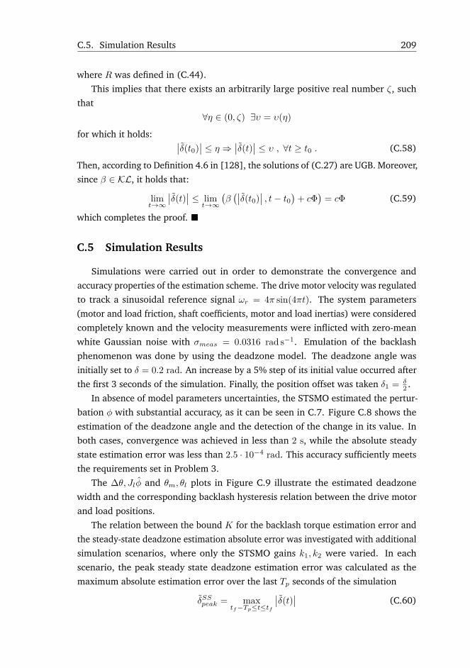
C.5. Simulation Results 209

where R was defined in (C.44).

This implies that there exists an arbitrarily large positive real number ζ, such

that

∀η ∈ (0, ζ) ∃υ = υ(η)

for which it holds: ∣∣δ(t0)∣∣ ≤ η ⇒

∣∣δ(t)∣∣ ≤ υ , ∀t ≥ t0 . (C.58)

Then, according to Definition 4.6 in [128], the solutions of (C.27) are UGB. Moreover,

since β ∈ KL, it holds that:

limt→∞

∣∣δ(t)∣∣ ≤ lim

t→∞

(β(∣∣δ(t0)

∣∣ , t− t0)

+ cΦ)

= cΦ (C.59)

which completes the proof.

C.5 Simulation Results

Simulations were carried out in order to demonstrate the convergence and

accuracy properties of the estimation scheme. The drive motor velocity was regulated

to track a sinusoidal reference signal ωr = 4π sin(4πt). The system parameters

(motor and load friction, shaft coefficients, motor and load inertias) were considered

completely known and the velocity measurements were inflicted with zero-mean

white Gaussian noise with σmeas = 0.0316 rad s−1. Emulation of the backlash

phenomenon was done by using the deadzone model. The deadzone angle was

initially set to δ = 0.2 rad. An increase by a 5% step of its initial value occurred after

the first 3 seconds of the simulation. Finally, the position offset was taken δ1 = δ2 .

In absence of model parameters uncertainties, the STSMO estimated the pertur-

bation φ with substantial accuracy, as it can be seen in C.7. Figure C.8 shows the

estimation of the deadzone angle and the detection of the change in its value. In

both cases, convergence was achieved in less than 2 s, while the absolute steady

state estimation error was less than 2.5 · 10−4 rad. This accuracy sufficiently meets

the requirements set in Problem 3.

The ∆θ, Jlφ and θm, θl plots in Figure C.9 illustrate the estimated deadzone

width and the corresponding backlash hysteresis relation between the drive motor

and load positions.

The relation between the bound K for the backlash torque estimation error and

the steady-state deadzone estimation absolute error was investigated with additional

simulation scenarios, where only the STSMO gains k1, k2 were varied. In each

scenario, the peak steady state deadzone estimation error was calculated as the

maximum absolute estimation error over the last Tp seconds of the simulation

δSSpeak = maxtf−Tp≤t≤tf

∣∣δ(t)∣∣ (C.60)


and Validation

0 1 2 3 4 5 6 7−1

−0.5

0

0.5

1

t in s

J lφ,

J lφ

inN

m

JlφJl φ

Figure C.7: Real and estimated backlash torque scaled by the load inertia Jl.

0 2 4 60

0.1

0.2

t in s

δ,δ

inra

d

δδ

0 2 4 6t in s

δin

rad

−5

0

5·10−4

0 2 4 60

0.1

0.2

t in s

δ,δ

inra

d

δδ

0 2 4 6t in s

δin

rad

−5

0

5·10−4

Figure C.8: (Left): Real and estimated change of deadzone angle. (Right): Estimation error.

−0.1 0 0.1−1

−0.5

0

0.5

1

∆θ in rad

J lφ

inN

m

0 0.5 1 1.5 20

1

2

δ

θm in rad

θ lin

rad

Figure C.9: (Left): Deadzone illustration through torque-position difference. (Right):

Backlash hysteresis.

C.6. Experimental Results 211

where tf denotes the end time of each simulation. The different obtained values for

δSSpeak were plotted against the corresponding bounds for Jl|φ|. Figure C.10 shows

the approximately linear relation between the two bounds, with a slope q ≈ 0.0023.

0.1 0.2 0.3 0.4 0.50

1

2

·10−3

limt→∞

∣∣δ(t)∣∣ = qK, q ≈ 0.0023

K in N m

δSS

pea

kin

rad

datalinear fit

Figure C.10: Linear relation between the bounds for the perturbation estimation error φ and

the deadzone angle estimation error δ.

C.6 Experimental Results

C.6.1 Experimental Setup

The experimental setup consists of two Siemens FT7042-5AF70 PMSMs con-

nected through a stainless steel shaft. Both motors are equipped with a Siemens

SINAMICS S120 drive converter with 11-bit absolute encoders for the position.

Three custom-made jaw couplings are mounted (one at a time) on a steel base

and house the two parts of the interconnecting shaft (see Figure C.12). The to-

tal deadzone angle for each of the couplings is 1.027 rad, 0.186 rad and 0.105

rad (58.8445, 10.6685 and 6.0161, respectively). The entire drive train with the

friction component are shown in Figure C.11.

The load motor (see Figue C.11) serves as a pure inertia in the experiments. The

design and tuning of the position, velocity and current control loops in the drive

motor were not included in this study.

C.6.2 Test Scenarios

The identified parameters of the physical system were used in the experiments

for the assessment of the estimation algorithm. Five more variation cases were

considered for testing the robustness and performance of the deadzone estimator


and Validation

Figure C.11: Experimental setup: (1) 1FT7 drive PMSM, (2) 1FT7 load PMSM, (3) shaft, (4)

backlash mechanism, (5) mounting base.

Figure C.12: Jaw coupling detail.

against parameter uncertainties. In each of these additional tests one of the four

uncertain parameters (shaft and friction coefficients) was increased by 100% of

their identified value. In the fifth test all four parameters (KS , DS , TC,l, βl) were

increased simultaneously. The reference for the position of the drive motor was a

sinusoid,


where in all the tests Θ0 = 1 rad and fr = 0.5 Hz. The fifteen different scenarios are

shown in Table C.2. The parameters of the identified physical system, as well as,

those of the SMO and adaptive estimator are collectively given in Table C.3.


Table C.2: Test scenarios.

No δ (rad) δ1 (rad) Parameter variation

0A 1.027 0.8924 No variation

1A 1.027 0.8924 100% increase in KS

2A 1.027 0.8924 100% increase in DS3A 1.027 0.8924 100% increase in TC,l4A 1.027 0.8924 100% increase in βl5A 1.027 0.8924 All variations combined

0B 0.186 0 No variation

1B 0.186 0 100% increase in KS

2B 0.186 0 100% increase in DS3B 0.186 0 100% increase in TC,l4B 0.186 0 100% increase in βl5B 0.186 0 All variations combined

0C 0.105 0.0021 No variation

1C 0.105 0.0021 100% increase in KS

2C 0.105 0.0021 100% increase in DS3C 0.105 0.0021 100% increase in TC,l4C 0.105 0.0021 100% increase in βl5C 0.105 0.0021 All variations combined

Table C.3: System and estimator parameters values.


STSMO parameters

k1 Switching gain 0.5k2 Integral switching gain 70

Estimator parameters

α Stiffness model slope 104

γ Adaptation gain 5 · 10−4

δ0 Initial conditions 0 radδmax Maximum deadzone 2π rad

Load system parameters

Jl Inertia 0.000831 kg m2

KS Shaft stiffness 31.75 N m rad−1

DS Shaft damping coefficient 0.054 N m s rad−1

N Gearing ratio 1TC,l Coulomb friction 0.0792 N mβl Viscous friction coefficient 0.031 N m s rad−1


and Validation

C.6.3 Results

This section presents the results obtained from the experiments on the estimation

of the deadzone angle. The performance of the estimator was evaluated based on

the MAEE, which is defined over a time interval T > 0 as

MAEE = supt0≤t≤t0+T

∣∣δ(t)∣∣ . (C.61)

Figure C.13 shows the estimation of the deadzone angle for the cases where the

identified parameters of the system were used (Tests 0A, 0B, 0C). As it can be seen,

the estimation error δ converges to a compact set including the origin, while the

corresponding MAEE is less than 10−2 rad in all the tests, specifically 1.75 · 10−3 rad,

1.90 · 10−3 rad and 0.66 · 10−3 rad for Test 0A, 0B and 0C, respectively.

0 50 100 1500

0.5

1

1.5

1.027

0.1860.105

t in s

δ,δ

inra

d

δδ

0 50 100 150

0

0.5

1

t in sδ

inra

d

Test 0ATest 0BTest 0C

−1012

·10−3

Figure C.13: Deadzone angle estimated value (left) and the associated estimation error

(right) for the nominal cases (Tests 0A, 0B, 0C).

The position of the motor and the load can be seen in figure C.14 (top). While

in the deadzone, the load does not move although the drive motor shaft does. This

loss of engagement is also shown in the bottom plot of the same figure, where the

connecting shaft stiffnes is depicted. Whenever the system is in the deadzone, the

shaft stiffness is 0. During the initial part of the motion in the positive direction

the stiffness it is zero even though the load is moving. This is due to the fact that

impact torque exerted by the drive motor on the load temporarily accelerates the

load, making it move even though there is no actual engagement.

An illustration of the estimated deadzone is given in Figure C.15, where the

backlash torque Jlφ estimate and the equivalent calculation based on the stiffness

model (top plot) are depicted as functions of the position difference between motor

and load. The oscillations at the two ends of the deadzone in the estimated torque


−1

0

1

θ m,θ

lin

rad

θmθl

150 151 152 153 1540

10

20

30

t in s

KB

Lin

Nra

d

Figure C.14: Motor and load position (top) and the calculated shaft stiffness (bottom) for

the nominal case with δ = 1.027 rad (Test 0A).

correspond to the impact between motor and load upon engagement. The bottom

plot in the same figure shows the stiffness KBL also as a function of ∆θ.The backlash hysteresis can be seen in the top plot of Figure C.16, which shows

4 s of the time response of the load position with respect to this of the motor. The

bottom plot shows the drive motor and load phase portraits, i.e. the plots of their

angular velocities with respect to their positions.

Figure C.17 illustrates the actual and estimated by the SMO load angular velocity

during Test 0A. As it can be seen in the bottom plot, the velocity estimation error

is smaller than 0.4 rad s−1 in magnitude. Such an error is sufficiently small, so that

the estimated backlash torque, shown in Figure C.18, can be considered accurate

enough to be used in the deadzone estimation algorithm.

The deadzone angle estimation error for all the parameter variations is show in

Figures C.19, C.20, C.21 (for Tests 1A-5A, 1B-5B and 1C-5C, respectively). As it

can be seen, in all the considered cases, the estimates converge to a constant value

sufficiently close to the real one. Specifically, all the estimation errors do not exceed

4 · 10−3rad in magnitude, which implies more than 40% better performance from

that required in Problem 3. The MAEE during all Tests are presented in Table C.4.

Remark C.4. The sudden engagement between drive motor and load produced a


and Validation

−0.4

−0.2

0

0.2

0.4J l

φ,T l

inN

SMOModel

−1 −0.8 −0.6 −0.4 −0.2 0 0.20

10

20

30

δ1

δ

∆θ in rad

KB

Lin

Nra

d

Figure C.15: Deadzone illustration through torque-position difference (top) and torque-

stiffness (bottom) plots during Test 0A.

−2 −1 0 1 2

0

0.5

1

δ

θm in rad

θ lin

rad

−2 −1 0 1 2

−4

−2

0

2

4

θm,θl in rad

ωm,ω

lin

rad

s−1

motorload

Figure C.16: Backlash hysteresis (left) and phase portraits for the motor and load (right)

during Test 0A.


−4

−2

0

2

4

ωl,

ωl

inra

ds−

1

ωlωl

4 4.5 5 5.5 6 6.5 7 7.5

−0.4

−0.2

0

0.2

0.4

t in sec

ωl

inra

ds−

1

−4

−2

0

2

4

ωl,

ωl

inra

ds−

1

ωlωl

4 4.5 5 5.5 6 6.5 7 7.5

−0.4

−0.2

0

0.2

0.4

t in sec

ωl

inra

ds−

1

Figure C.17: Real and estimated load velocity (top) and the associated estimation error

(bottom) during Test 0A.

150 151 152 153 154

−0.4

−0.2

0

0.2

0.4

t in s

J lφ

inN

Figure C.18: Estimated backlash torque for the nominal case with δ = 1.027 rad (Test 0A).

Table C.4: MAEE in mrad for the nominal case (Tests 0A, 0B, 0C) and all the parameter

variations (Tests 1A-5A, 1B-5B, 1C-5C).

MAEE in mradδ in rad 0 1 2 3 4 5

1.027 (case "A") 1.75 0.41 1.80 3.61 2.69 1.850.186 (case "B") 1.90 1.04 1.87 3.31 1.96 1.800.105 (case "C") 0.66 1.85 0.72 1.38 0.57 0.93


and Validation

0 20 40 60 80 100 120 140−0.5

0

0.5

1

1.5

t in s

δin

rad

Test 1A Test 2ATest 3A Test 4ATest 5A

0

2

4

·10−3

Figure C.19: Deadzone angle estimation error during Tests 1A-5A.

0 20 40 60 80 100 120 140

0

0.2

0.4

t in s

δin

rad

Test 1B Test 2BTest 3B Test 4BTest 5B

0

2

4

·10−3

Figure C.20: Deadzone angle estimation error during Tests 1B-5B.

0 20 40 60 80 100 120 140−0.1

0

0.1

0.2

t in s

δin

rad

Test 1C Test 2CTest 3C Test 4CTest 5C

−2

0

2·10−3

Figure C.21: Deadzone angle estimation error during Tests 1C-5C 4.

C.7. Conclusions 219

periodic impact torque acting on both parts. This caused a small displacement of the

load, which resulted in an shift of the position offset δ1. However, the effect of this

change in the offset on the quality of the estimation was practically negligible.

C.7 Conclusions

A deadzone angle estimation method for a single-axis drive-train with backlash

was presented in this paper. The design is a modified version of the cascaded SMO-

adaptive estimator scheme presented in [4], which now includes an initial position

offset between drive motor and load. The stability and robustness properties of

the algorithm were discussed in the context of model and parameter uncertainties.

Specifically, it was proven that the estimation error is UGAS in absence of model and

parameter mismatches and UGB otherwise, with the bound being proportional to

the total perturbation estimation error bound.

The theoretical findings were experimentally validated on a real single-axis drive

train with state-of-the-art Siemens equipment for the cases where the deadzone

was equal to 1.027 rad, 0.186 rad and 0.105 rad. The method was tested both for

the identified system parameters and for the case of 100% offset in each of these

parameters. In all the tests convergence was achieved in approximately 40 s and

with precision in the order of 10−3 rad.

Future work will include the assessment of the algorithm performance in estima-

ting even smaller angles and also the design of an joint estimation scheme for both

the deadzone angle and the initial position offset.

Acknowledgements

The sponsorship of this project by Siemens AG is gratefully acknowledged.

Paper D

Backlash Estimation for IndustrialDrive-Train SystemsDimitrios Papageorgiou*1, Mogens Blanke2, Hans Henrik Niemann1, Jan H. Richter3






Abstract:

Backlash in gearing and other transmission components is a common positioning-

degrading phenomenon that develops over time in industrial machines. High-

performance machine tool controls use backlash compensation algorithms to main-

tain accurate positioning of the tool to cope with such deadzone phenomena. As

such, estimation of the magnitude of deadzones is essential. This paper addresses the

generic problem of accurately estimating the width of the deadzone in a single-axis

mechanical drive train. The paper suggests a scheme to estimate backlash bet-

ween motor and load, employing a sliding-mode observer and a nonlinear adaptive

estimator. The efficacy of the approach is illustrated via simulations.


222 Paper D. Backlash Estimation for Industrial Drive-Train Systems

D.1 Introduction

Developing backlash due to wear in spindles, gears, clutches and guides is one of

the main reasons for performance degradation in machine tool systems. Since high

precision tool positioning is fundamental for obtaining the required quality of the

machined end-products, backlash compensation is used in nearly all modern CNC

algorithms. Compensation necessitates knowledge of the backlash offset angle so that

it can be used in the position servo loops that control motors on the machine’s axes.

In such context, online estimation methods may facilitate automatic compensation

for developing backlash.

A substantial amount of research has been conducted on estimation of the

backlash phenomenon for various systems over the past three decades. In [51] the

backlash in a gearing system was indirectly estimated by calculating the bounce, i.e.

the change of the speed of the driving part of the gear due to the backlash impact

when exiting the deadzone. EKF was employed in [52] for estimating a backlash

torque in a two-mass motor arm, based on torque and position measurements.

Modelling of backlash torque was presented in [47], who used a differentiable

function to represent backlash and suggested a nonlinear observer for estimation of

backlash amplitude. This method was validated experimentally in [57], in which

a sliding-mode observer was used for estimation of backlash torque. Based on this

estimation, backlash function parameters were identified offline. The effect of the

deadband due to backlash in a closed loop motion system was studied in [54] using

describing functions. The function parameters were calculated online using a static

relation for controller gains. Backlash in automotive powertrains was described in

[53] based on position difference between drive motor and load. A Kalman filter

was shown to estimate backlash within 10% error. A four-parameter model was used

in [55] to describe backlash effects in generic linear cascaded systems. The backlash

identification was treated as a quasi-linear problem such that iterative algorithms

could be used. Minimization of a quadratic prediction error was employed in [56],

where position, velocity and torque measurements were used for offline identification

of backlash torques in a vehicle drive-line system.

In the previous approaches, the backlash phenomenon was described through

the resulting torque upon contact of two parts of a coupling. In the cases where the

deadzone angle was identified directly, this was done offline or around a linearization

point of the system. The previous results showed the need for new ideas for high

accuracy estimation of backlash if compensation shall be useful in machinery systems

where very high precision is required.

This paper considers the problem of designing a dynamic estimator for the

D.2. System Description and Problem Formulation 223

deadzone angle of a developing backlash in a single-axis drive-train system. The

proposed method employs modelling of backlash in terms of variable shaft stiffness,

depending on the deadzone size, and it addresses the requirement for fast and

accurate estimation of the deadzone angle. Similarly to [57], a second order STSMO

is used to estimate the backlash torque. This value is utilized by an adaptive estimator

designed with the purpose to determine the deadzone angle.

The paper is organized as follows: Section D.2 states the problem in concise

terms, describing the drive-train system as an abstraction of a single-axis machine

tool, and presents a model for backlash based on varying shaft stiffness. The design

of the parameter estimator is presented in Section D.3 and Section D.4 presents

results obtained from high fidelity simulations. Finally, conclusions are drawn and

results are discussed in Section D.5.

D.2 System Description and Problem Formulation

A typical single-axis machine tool consists of a linear axis, which positions the

tool. The axis is actuated by a drive motor that is typically connected to an angular-

to-linear motion conversion device (e.g. a ball-screw).

Drive motorJm


Linear axisdynamics

Generalized loadωl

Figure D.1: Correspondence between mechanical drive-train and single-axis machine-tool

systems. The angular velocities of the motor and the load are denoted by ωm, ωl, respectively,

while υT is the tool linear velocity.

The combined elasticity, friction, damping and total mass of all the mechanical

components that connect to the drive shaft can be lumped into a generalised load.

The single-axis machine tool can then be viewed as a mechanical drive train compri-

sing the drive motor, a flexible shaft with damping and backlash, and a load with

friction as show in Figure D.1.

D.2.1 Drive Train Modelling

With identification of backlash being in focus of this work, angular accelerations,

velocities and difference of angles between mechanical components are essential.

Torque produced by the drive motor is measured, hence the closed-loop electrical


dynamics of the motor need not be considered. An overview of the most important

variables and notation used in the modelling of the system is provided in Table D.1.

Table D.1: System model nomenclature


States and Outputs

ωm, ωl Motor/load angular velocity rad s−1

θm, θl Motor/load angular position radInputs and disturbances

u Torque command N mTF,m, TF,l Motor/load friction N m

Tl Interconnection/backlash torque N mConstant parameters

Jm, Jl Motor/load inertia kg m2



N Gearing ratio −TC,m, TC,l Coulomb friction on the motor/load N mβm, βl Motor/load viscous friction coefficient N m s rad−1

δ Deadzone angle rad

The dynamics of the mechanical drive-train system reads:

ωm = 1Jm

u− 1Jm

TF,m −1

NJmTl (D.1)

θm = ωm (D.2)

ωl = − 1JlTF,l + 1

JlTl (D.3)

θl = ωl . (D.4)

In the backlash-free case the interconnecting torque Tl is given from:

Tl = KS

(1Nθm − θl

)+DS

(1Nωm − ωl

)(D.5)

where KS , DS and N are defined in Table D.1 and are assumed to be known. The

friction torques acting on the drive motor and the load are modelled as described in

the following equation ([30]):

TF,i = TC,isgn(ωi) + βiωi, i ∈ m, l (D.6)

D.2. System Description and Problem Formulation 225

where sgn : R→ −1, 0, 1 is the signum function defined as:

sgn(ξ) =

1 if ξ > 0

υ ∈ [−1, 1] if ξ = 0

−1 if ξ < 0 .

(D.7)

and the parameters βm, βl, TC,m, TC,l are considered known and constant.

D.2.2 Backlash Modelling

Backlash is the effect of sudden disengagement between drive motor and load as

shown in Figure D.2. A number of static and dynamic models have been developed,

based on the interconnecting (restoring and damping) torque in a mass-spring-

damper system (see for example [45, 48, 50] and [49]). The most intuitive and

common one is the deadzone model presented by [45], in which the interconnecting

torque Tl becomes zero inside the deadzone, while outside of it the angle difference

(between motor and load) is offset by the width of the deadzone angle.

Figure D.2: Backlash: When the difference between the motor and the load position is smaller

than δ, then the two shafts are disengaged and no torque is applied to the motor or the load.

The picture is taken from [49].

Although the existing backlash models can accurately describe the phenomenon,

the discontinuities that they contain make these models difficult to use in control

and estimation design. A model for backlash, which is based on changing shaft

stiffness, will be presented in this section and compared to the deadzone model.

This model will subsequently be used for deadzone estimation and monitoring.

Defining the angular position and velocity differences between drive motor and

load as

∆θ , 1Nθm − θl (D.8a)

∆ω , 1Nωm − ωl (D.8b)


the interconnection torque Tl in the deadzone model is given by

TDZl =

KS(∆θ − δ · sgn(∆θ)) +DS∆ω , |∆θ| > δ

0 , |∆θ| ≤ δ .(D.9)

The proposed model is based on factorization of the backlash torque as a function

of shaft stiffness. The latter is very small, virtually zero, when inside the deadzone,

and assumes its nominal value outside of it. The transition between the two extreme

values of the stiffness is fast but smooth. The corresponding torque reads:

Tl =[∆θ − δ · sgn(∆θ) + DS

KS∆ω]·KBL(∆θ, δ) (D.10)

KBL = KS

π[π + arctan(α(∆θ − δ))− arctan(α(∆θ + δ))] (D.11)

The positive constant α expresses the rate of change in the stiffness as it can be seen

in Figure D.3. For α→∞, it is clear that Tl → TDZl .

−0.04 −0.02 0 0.02 0.04

0

0.2

0.4

0.6

0.8

1

·104

∆θ in rad

KB

Lin

Nm

rad−

1

KS

α = 700α = 103

α = 2 · 103

α = 104

−0.04 −0.02 0 0.02 0.04

0

0.2

0.4

0.6

0.8

1

·104

∆θ in rad

KB

Lin

Nm

rad−

1

KS

α = 700α = 103

α = 2 · 103

α = 104

−0.04 −0.02 0 0.02 0.04

0

0.2

0.4

0.6

0.8

1

·104

∆θ in rad

KB

Lin

Nm

rad−

1

KS

α = 700α = 103

α = 2 · 103

α = 104

Figure D.3: Shaft stiffness varying between two values. The larger the value of α, the steeper

the change in the stiffness is.

D.2.3 Problem Formulation

The collective objective can be summarised in the following problem formulation:

D.3. Backlash Deadzone Angle Estimation 227

Problem C (Deadzone angle estimation). Given the single-axis drive-train sy-stem described in (D.1)-(D.6) and the backlash model in (D.10),(D.11), designan online dynamic estimator for the deadzone angle δ with the following require-ments:

• Maximum steady-state estimation error less than 10−3 rad.

• Asymptotic convergence to the real parameter value.

D.3 Backlash Deadzone Angle Estimation

Estimation of the deazone angle belongs to a family of problems of online

parameter estimation in systems with nonlinear parametrization that has been

treated in numerous works in the literature. The approach followed in this paper is

based on a method for parameter estimation in nonlinearly parametrized systems

presented in [122]. The basic idea relates to estimating a perturbation of the system

dynamics that depends on the unknown parameter and then finding an adaptive law

for estimating the parameter itself.

D.3.1 Method Overview

Consider that the system dynamics is described by

x = f(x) + g(x) [u(x) + d(x, δ)] (D.12)

where x ∈ Rn is measured, f : R≥0 × Rn → Rn and g : R≥0 × Rn → Rn×m are

the unforced system dynamics and gain, respectively, which can be evaluated from

the measurements, δ ∈ D ⊂ R is the unknown parameter, u ∈ Rm is the control

input and d : R≥0 × Rn ×D → Rm is a matched disturbance vector, which can be

evaluated if δ is known. The method pertains to finding an estimation φ of the

perturbation

φ , g(x)d(x, δ) (D.13)

and then derive an adaptive law

˙δ = ρ(x, φ, δ) (D.14)

for estimating the unknown parameter.

Regarding the drive-train system, all states are measured and the unknown

parameter δ affects the dynamics of both the motor and the load in the same way,


i.e. through the torque Tl. We can then choose either of the subsystems in (D.1),

(D.3) on which to apply the method. For simplicity, the load velocity dynamics is

chosen. The system can be written in the form of (D.12) with

f(x) ≡ f(ωl) = 1JlTF,l

g(x) ≡ g = 1Jl

d(x, δ) = Tl ,

where Tl has been defined in (D.10), (D.11) and

x ,[ωm θm ωl θl

]T

is the state vector of the drive-train system. The method is divided in two parts:

estimation of the perturbation φ and derivation of the adaptive law ρ(x, φ, δ).

D.3.2 Sliding-Mode Perturbation Observer

A second-order SMO was used for finding an estimate of φ. In general SMOs can

offer finite-time estimation of unmeasured states by using high-frequency injection

signals in their design, which depend on the observer innovation term (i.e. the error

between real and predicted output) as shown in [61]. By doing so, the estimation

error dynamics reaches the sliding manifold, i.e. a manifold on which the error and

its first time derivative are zero, and remain so thereafter. This provides at the same

time an estimation of any unknown perturbations that affects the system dynamics

([79]). This idea can be clarified as follows.

Consider the load velocity dynamics presented in (D.3) and a SMO given by

˙ωl = − 1JlTF,l + v(ωl) (D.15)

where ωl = ωl − ωl is the state estimation error and v is an appropriate high

frequency term depending on the error signal ωl. Define the sliding manifold

S =ωl ∈ R : ωl = ˙ωl = 0

. The dynamics of the state estimation error reads:

˙ωl = ωl − ˙ωl = 1JlTl − v . (D.16)

If the error dynamics reaches the sliding manifold, then ˙ωl = ωl = 0 for all

future times, which means that v = 1JlTl. In other words, if the injection signal v

is designed such that the estimation error dynamics reaches the sliding manifold Sand remains on the manifold thereafter, then the unknown perturbation φ = 1

JlTl is

estimated indirectly by v. The design of v can be obtained as in [70]:


∫ t

0sgn(ωl(τ))dτ (D.17)

D.3. Backlash Deadzone Angle Estimation 229

where k1, k2 are positive gains. The resulting observer is referred to as the STSMO

and it is proven in [124] that for appropriate gains k1, k2, the term v brings the ob-

server error dynamics onto the sliding manifold S. Hence, the unknown perturbation

can be estimated by (D.17), where


∫ t

0sgn(ωl(τ))dτ . (D.18)

The choice of a second order SMO for a system of relative degree 1 (the subsystem

is scalar) was made due to the property of higher order SMOs to alleviate the

chattering in the injection and estimation signals ([61]).

Remark D.1. Finite-time estimation of φ is ensured by selecting v as in (D.17) with

k1, k2 being appropriately chosen positive gains. One additional requirement is that

Tl, Tl need be bounded, which is ensured by the boundedness of the state vector and

the smoothness of the backlash model. However, the bound on Tl is proportional to

α. This means that the closer the model is to the deadzone model, the larger this

bound will be, which in turn leads to higher gains for the observer.

D.3.3 Adaptive Backlash Angle Estimator

The estimator design is inspired by the method proposed in [122] for the esti-

mation of unknown parameters. For the rest of the analysis we consider that the

unknown parameter δ lies in a compact set D ⊂ R, with δ = 0 and we define the

backlash angle estimation error as δ = δ − δ.Considering the dynamics of the load velocity expressed in the form of (D.12)

with g = 1Jl

and d(x, δ) = Tl(x, δ) defined in (D.9),(D.11), the adaptive estimator

for the deadzone angle is given by ([122]):


[δ, γµ(x, δ)

(φ− 1

JlTl(x, δ)

)](D.19)

with γ > 0 being the adaptive gain, φ an asymptotic estimate of 1JlTl and Proj(·, ·)

the projection operator defined in (II.6). In the adaptive law (D.19) µ(x, δ) is a

real-valued function defined on R4 ×D, bounded for bounded x, with the following

property:

Property D.1. For all pairs δ1, δ2 ∈ D and ∀x ∈ R,

µ(x, δ1) 1Jl

∂Tl∂δ

(x, δ2) ≥ σ(x) (D.20)

where σ(x) is a non-negative real-valued function defined on R4 with the follo-

wing two properties:


Property D.2. There exists a positive real constant number L > 0 such that ∀δ1, δ2 ∈ D,

1Jl|Tl(x, δ)− Tl(x, δ)| ≤ L

√σ(x)|δ| . (D.21)

Property D.3. There exist positive real numbers T, ε such that ∀t ∈ R≥0,∫ t+T

t

σ(x(τ))dτ ≥ ε . (D.22)

Following a similar reasoning as the one in the proof of Proposition 4 in [122],

it can be shown that the estimation error δ converges asymptotically to 0, and

uniformly in x if an asymptotic estimate of φ is available.

The design of the adaptive deadzone angle estimator includes steps to find

suitable functions µ and σ with the properties (D.1)-(D.3). Selecting µ(x, δ) as

µ(x, δ) = 1K2S

∂Tl∂δ

(x, δ) (D.23)

condition (D.20) is satisfied with

σ(x) = 1K2S

(∂Tl∂δ

)2= 1π2

[χ1(x, δ) + χ2(x, δ)

]2(D.24)


χ1(x, δ) = sgn(∆θ)[π + arctan(α(∆θ − δ))− arctan(α(∆θ + δ))

](D.25)

χ2(x, δ) =[∆θ − δ · sgn(∆θ) + DS

KS∆ω]

α

1 +[α(∆θ − δ)

]2 + α

1 +[α(∆θ + δ)

]2

.

(D.26)

Since x and σ(x) are bounded and D is compact, it is easy to show that there

exits L > 0, such that condition (D.21) holds. The inequality∫ t+Tt

σ(x(τ))dτ ≥ ε

expresses a type of PE condition. From (D.24)-(D.26) it can be seen that this

condition does not hold if, during the time interval [t, t+ T ], the system is always

within the deadzone. This, however, is expected, since in that case, there is no

engagement between motor and load, hence no information about the stiffness of

the shaft that connects them.

The adaptive law for the parameter estimate δ is finally given by:

˙δ = Proj

δ, γ

1K2S

∂Tl∂δ

(x, δ)[φ− 1

JlTl(x, δ)

], γ > 0 (D.27)

where∂Tl∂δ

(x, δ) = −KS

π

[χ1(x, δ) + χ2(x, δ)

]. (D.28)

D.4. Simulation Results 231

Remark D.2. By using the STSMO in (D.15), (D.17), we ensure that φ will converge

to the real perturbation φ in finite-time, which is a stronger convergence property

than the one required by the adaptive estimator. However, the effect of measurement

noise and parameter or model uncertainties (e.g. in friction) may compromise

the exact estimation of φ. In this case, by using arguments from the stability of

interconnected systems, one can show that the deadzone angle estimation error will

not converge asymptotically to zero but it will reach a compact set [δ − eδ, δ + eδ],where 0 < eδ ≤ c|φ− φ|, c > 0.

Remark D.3. It is interesting to note that the selection of the specific µ(x, δ) function

results into a gradient-type adaptive law, which is very common in the literature

of adaptive techniques. Although for nonlinearly parametrized systems it does not

always guarantee parameter convergence as it does for linear-in-the-parameters

systems, it is a natural first choice for the adaptive law.

The complete estimator design is summarized in the following algorithm:

Algorithm 1 Backlash angle estimationMeasured: State variables ωm, θm, ωl, θl .


1: Design a STSMO for the load velocity (Equations (D.15), (D.17)).

2: Estimate the backlash torque (Equation (D.18)).

3: Design the adaptive estimator for the deadzone angle δ (Equations (D.25)-

(D.28)).

D.4 Simulation Results

The drive-train system described in Equations (D.1)-(D.5) was simulated in

Matlab to assess the performance of the estimation algorithm. The deadzone model

in (D.9) was used to emulate the backlash phenomenon. A PI controller was used

to regulate the drive motor velocity into following a sinusoidal profile ωrefm =Ω sin(νt). A 5% change in the deadzone angle was considered for the evaluation of

the algorithm. The velocity measurements were afflicted with white Gaussian noise

w ∼ N (0, σ2meas). High precision absolute position encoders were used and the error

due to quantization was ignored. Table D.2 shows the values of the constants used

for the simulations. The compact set D is the real axis interval [0, 1], the estimator

was initialized at δ(0) = δ0, γ was chosen to be 0.1 and the sampling time was 2 ms.Figure D.5 shows the real torque applied in the system according to the deadzone

model and its estimation by the STSMO. A small lag can be observed in the estimation


Motor dynamics

Eq. (C.1),(C.2)u

Interconnection

system Eq. (C.5)

ωm θm

Tl

Load dynamics

Eq. (C.3),(C.4)

ωl θl

Load velocity

observer Eq.

(C.15),(C.17),(C.18)

ωl

Backlash Model

Eq. (C.10),(C.11)

J−1l

Tl(x, δ )

φ +− Deadzone angle

estimator Eq.

(C.25)-(C.28)

δ

Single-axis System

x

Figure D.4: Block diagram of the closed-loop mechanical drive-train system and the estima-

tion scheme.

Table D.2: Values used in the simulations

Symbol Value Units

Jm, Jl 8.31 · 10−4 kg m2

KS 31.7557 N m rad−1

DS 0.0038 N m s rad−1

α 105 −N 1 −TC,m, TC,l 0.0492 N mβm, βl 0.0008 N m s rad−1

k1 32.712 −k2 12.0154 −δ0 0.02 radγ 0.1 −δ1 0.1 radδ2 0.105 radΩ 10 rad s−1

ν 24/(2π) rad s−1

σmeas 0.0316 rad s−1

D.5. Conclusions 233

of φ, which, however, does not affect the performance of the algorithm. Increasing

the gains k1, k2 of the observer reduces the delay in estimation but makes the method

more sensitive to measurement noise.

0 1 2 3 4 5−1

−0.5

0

0.5

1

t in s

Jlφ,J

lφin

Nm

Jlφ

Jlφ

Figure D.5: Real and estimated backlash torque scaled by the load inertia Jl.

The real and estimated deadzone angle, as well as the estimation error, are

shown in Figure D.6. The plots show that the deadzone angle is estimated with

sufficient accuracy in less that 2 s. Specifically, the average steady state estimation

error is less than 10−3 rad, which the order of magnitude for positioning precision

in machine tool applications [18]. Larger sensor noise has a direct impact on the

speed of convergence and the steady-state deviation.

D.5 Conclusions

A method for deadzone angle estimation in a single-axis drive-train with backlash

has been presented in this paper. The interconnecting torque acting on motor and

load was first estimated using a STSMO, followed by an adaptive algorithm that

was designed to estimate deadzone angle. The method was tested in a simulation

framework, where the adaptive estimator was able to track the real value of the

deadzone angle, as well as a 5% increase in the backlash. The parameter convergence

was achieved in less than 2 s with precision in the order of 10−3 rad. Such precision

will allow for use of the estimated parameter in backlash compensation algorithms,

that are used in many machine-tool controls. Moreover, detection of changes in the


0 2 4 60

0.05

0.1

t in s

δ,δ

inra

d

δδ

0 2 4 6

0

0.05

0.1

t in s

δin

rad

0 2 4 60

0.05

0.1

t in s

δ,δ

inra

d

δδ

0 2 4 6

0

0.05

0.1

t in s

δin

rad0 2 4 6

0

0.05

0.1

t in s

δ,δ

inra

d

δδ

0 2 4 6

0

0.05

0.1

t in s

δin

rad

Figure D.6: (Left): Real and estimated change of deadzone angle. (Right): Estimation error.

deadzone angle can infer a measure of wear in the mechanical components (i.e.

gearing, ball screw, couplings or guides) of the system.

Experimental validation of the method is ongoing.

Acknowledgements

The project is sponsored by Siemens AG.

Supplementary MaterialI The dq0 Transformation

In applications where high accuracy and acceleration are required and, thus,

torque-current control of PMSMs is essential, it is convenient to utilize a different

description of the 3-phase quantities of the motor (currents and voltages). This

alternative description, referred to as the dq0 transformation, is given by [125]

fd

fq

f0

= 2

3

cos(θ) cos(θ − 2π

3)

cos(θ + 2π

3)

− sin(θ) − sin(θ − 2π

3)− sin

(θ + 2π

3)

12

12

12

fa

fb

fc

(I.1)

where f can be voltage, current or magnetic flux. For balanced 3-phase PMSMs,

such as the Siemens 1FT7, the f0 component is always zero.

With this transformation the effect of all electrical currents (and voltages) of the

motor is analysed in two components, namely the magnetizing current, also referred

to as the direct axis current, id (direct axis voltage Vd) and the torque current or

quadrature axis current, iq (similarly, quadrature axis voltage Vq) as shown in Figure

D.7. The magnetizing current is responsible for the generation of the magnetic field

of the stator, whereas the quadrature axis current is responsible for the generation

of the torque due to the interaction of the two magnetic fields (of the stator and the

rotor).

The reason for choosing the dq-frame description is because the sinusoidal nonli-

nearities induced by the alternating input voltages to the model are removed and

the inputs can be considered as if they were DC (i.e. only their amplitudes are

considered). This allows for independent control of the motor torque from the flux

of the magnetic field of the stator, which is the basic principle of vector control [125],

typically employed in highly-dynamic industrial application, such as machine tools.

II Basic Definitions

Definition 2 (signum function). The signum function sgn(·) is defined as:

sgn(y) =

1 if y > 0

υ ∈ [−1, 1] if y = 0

−1 if y < 0

. (II.1)


a

b

c

V

d

q

Vd

Vqωt

d

q

Va

Vb Vc

Figure D.7: Analysis of three-phase voltages in the dq−frame. The three phases Va, Vb, Vc are

combined in one vector V which rotates at the frequency of the phases. V is then analysed in

two normal components Vd, Vq on a frame that rotates with the same angular velocity ω.

Definition 3 (Pseudoinverse of a real matrix). The left pseudoinverse of a realmatrix A are respectively defined as [134]:

A+ =(ATA

)AT . (II.2)

Similarly, the right pseudoinverse of A is given by:

A+ = A(ATA

). (II.3)

Definition 4 (PE [82]). A piecewise continuous signal vector φ : R+ → Rn isPersistently Exciting with a level of excitation α0 > 0 if there exist constants α1, T0 > 0such that

α0I ≤1T0

∫ t+T0

t

φ(τ)φT (τ)dτ ≤ α1I . (II.4)

Definition 5 (The error function). The error function erf(·) is defined as:

erf(y) = 2√π

∫ y

0e−τ

2dτ. (II.5)

For implementation purposes, the error function can be approximated by the hyper-

bolic tangent function, i.e.

erf(y) ≈ tanh(y) = ey − e−yey + e−y

.

Definition 6 (The Projection operator [99]). Let Ωl be a convex subset of theparameter space D defined as

Ωc , δ ∈ D|h(δ) ≤ l ,

III. Elements of Lyapunov Stability Theory 237

where δ is the unknown parameter vector, l is a positive real constant and h : D → R isa smooth convex function. The projection operator is defined as follows:

Proj(δ, τ) =

τ , h(δ) < 0

τ , h(δ) ≥ 0 & ∇hT τ ≤ 0

τ − ∇h|∇h|

⟨∇h|∇h| , τ

⟩h(δ) , h(δ) ≥ 0 & ∇hT τ > 0

, (II.6)

where the convex function h has been chosen according to [99]:

h(δ) , (εδ + 1)δTδ − δ2

max

εδδ2max

. (II.7)

In the above definition of h, δmax is a conservative upper bound for ‖δ‖∞ and εδ is

a small positive number. The operator 〈·, ·〉 denotes the inner product.

Definition 7 (K,K∞ functions [128, Def. 4.2]). A continuous function α : [0, a)→(0,∞] is said to belong to class-K if it is strictly increasing and α(0) = 0. It is said tobelong to class-K∞ if a =∞ and α(r)→∞ as r →∞.

Definition 8 (KL,KL∞ functions [128, Def. 4.3]). A continuous function β :[0, a)× (0,∞] → (0,∞] is said to belong to class-KL (respectively KL∞) if, for eachfixed s, the mapping β(s, r) belongs to class-K (respectively K∞) with respect to r and,for each fixed r, the mapping β(r, s) is decreasing with respect to s and β(r, s)→ 0 ass→∞.

III Elements of Lyapunov Stability Theory

Definition 9 ([83, Def. A.4, p. 490]). Consider the system

x = f(t,x) (III.1)

where the function f : [0,∞) × D → Rn with D ⊂ Rn is locally Lipschitz in x andpiecewise continuous in t. The equilibrium point x∗ = 0 of the system (III.1) is:

• uniformly stable, if there exists a class-K function γ(·) and a positive constant c,independent of t0, such that

‖x(t)‖ ≤ γ(‖x(t0)‖), ∀t ≥ t0 ≥ 0, ∀x(t0) with ‖x(t0)‖ < c ; (III.2)

• uniformly asymptotically stable, if there exists a class-KL function β(·, ·) and apositive constant c, independent of t0, such that

‖x(t)‖ ≤ β(‖x(t0, t− t0)‖), ∀t ≥ t0 ≥ 0, ∀x(t0) with ‖x(t0)‖ < c ; (III.3)


• exponentially stable, if (III.3) is satisfied with β(r, s) = kre−as k, a > 0 ;

• globally uniformly stable, if (III.2) is satisfied with γ ∈ K∞ for any initial statex(t0) ;

• globally uniformly asymptotically stable, if (III.3) is satisfied with β ∈ KL∞ forany initial state x(t0) ;

• globally exponentially stable, if (III.3) is satisfied for any initial state x(t0) andwith β(r, s) = kre−as k, a > 0.

Lemma (Barbalat’s lemma [83, Lem. A.6, p. 491]). Consider the function φ :[0,∞)→ R. If φ is uniformly continuous and lim

t→∞

∫∞0 φ(τ)dτ exists and is finite, then

limt→∞

φ(t) = 0 .

Corollary ([83, Col. A.7, p. 491]). Consider the function φ : [0,∞) → R. Ifφ, φ ∈ L∞ and φ ∈ Lp for some p ∈ [1,∞), then

limt→∞

φ(t) = 0 .

Theorem (LaSalle-Yoshizawa [83, Th. A.8, p. 492]). Let x∗ = 0 be an equilibriumpoint of the system (III.1), where D = R and is f locally Lipschitz in x uniformly in t.Let also V : [0,∞)× Rn → [0,∞) be a continuously differentiable function such that

γ1(x) ≤ V (t,x) ≤ γ2(x)

V = ∂V

∂t+ ∂V

∂xf(t,x) ≤ −W (x) ≤ 0

∀t ≥ 0, ∀x ∈ Rn, where γ1, γ2 are class-K∞ functions and W is a continuous function.Then, all solutions of (III.1) are globally uniformly bounded and satisfy

limt→∞

W (x(t)) = 0 .

In addition, if W (x) is positive definite, then the equilibrium x∗ = 0 is globallyuniformly asymptotically stable.

Theorem ([128, Th. 4.10, p. 154]). Let x∗ = 0 be an equilibrium point for (III.1)

and D ⊂ Rn be a domain containing x∗ = 0. Let also V : [0,∞) × D → R be acontinuously differentiable function such that

k1‖x‖a ≤ V (t,x) ≤ k2‖x‖a

∂V

∂t+ ∂V

∂xf(t,x) ≤ −k3‖x‖a

∀t ≥ 0 and ∀x ∈ D, where k1, k2, k3 and a are positive constants. Then, x∗ = 0is exponentially stable. If the assumptions hold globally, then x∗ = 0 is globallyexponentially stable.

IV. Proof of ISS Property of eθ (I&I-AC) 239

Definition 10 (Input-to-State Stability [128, Def. 4.7, p. 175]). Consider thesystem

x = f(t,x,u) (III.4)

where f : [0,∞)× Rn × Rm → Rn is piecewise continuous in t and locally Lipschitzin x and u. The input u is a piecewise continuous, bounded function of t for allt ≥ 0. The system (III.4) is said to be ISS with respect to the input u if there exist aclass-KL function β and a class-K function γ such that for any initial state x(t0) andany bounded input u(t), the solution x(t) exists for all t ≥ t0 and satisfies

‖x(t)‖ ≤ β(‖x(t0)‖, t− t0) + γ

(sup lim

t0≤τ≤t‖u(τ)‖

). (III.5)

Theorem ([128, Th. 4.19, p. 176]). Consider the system (III.4). Let also V :[0,∞)× Rn → R be a continuously differentiable function such that

α1(‖x‖) ≤ V (t,x) ≤ α2(‖x‖)∂V

∂t+ ∂V

∂xf(t,x,x) ≤ −W3(x), ∀‖x‖ ≥ ρ(‖x‖) > 0

∀(t,x,u) ∈ [0,∞) × Rn × Rm, where α1, α2 are class-K∞ functions, ρ is a class-Kfunction and W3(x) is a continuous positive definite function on Rn. Then, the system(III.4) is input-to-state stable with γ = α−1 α2 ρ (see Definition 10).

Lemma ([128, Lem. 4.7, p. 180]). Consider the system

x1 = f1(t,x1,x2) (III.6a)

x2 = f2(t,x2) (III.6b)

where f1 : [0,∞) × Rn1 × Rn2 → Rn1 and f2 : [0,∞) × Rn2 → Rn2 are piecewise

continuous in t and locally Lipschitz in x ,[x1 x2

]T. Suppose that both x1 =

f1(t,x1, 0) has a globally uniformly asymptotically stable equilibrium point at itsorigin. Then, if the system (III.6a), with x2 as input, is input-to-state stable andthe origin of (III.6b) is globally uniformly asymptotically stable, the the origin of thecascade system (III.6a) and (III.6b) is globally uniformly asymptotically stable.

IV Proof of ISS Property of eθ (I&I-AC)

Define the continuously differentiable function Ve(eω) = 12Jme

2ω for which the


α1(|eω|) ≤ Ve ≤ α2(|eω|)


with α1(x) = 14y

2 and α2(y) = x2 being class K∞ functions. Taking the time

derivative of Ve along the trajectories of the error system in (A.52) yields

Ve = −kIIe2ω − eωφ(ωm)φT (ωm)z ≤ −kII |eω|2 + |eω| · λmax

(φ(ωm)φT (ωm)

)|z|

= −kII(1− λ)|eω|2 − |eω|[kIIλ|eω| − λmax

(φ(ωm)φT (ωm)

)|z|]

≤ −kII(1− λ)|eω|2 , α4(|eω|) , ∀|eω| ≥λmax

(φ(ωm)φT (ωm)

)

kIIλ|z| , α3(|z|)

where λmax(·) denotes the largest eigenvalue of a real matrix, 0 < λ < 1, α4(·) is a

class K∞ function and α3(·) is positive definite in R. Then according to Theorem

4.19 in [128, p. 176] the system in (A.52) is ISS with respect to the input z.

V Proof of ISS Property of eθ (ABSC)

Define the continuously differentiable function Ve(eθ) = 12e

2θ for which the


α1(|eθ|) ≤ Ve ≤ α2(|eθ|)

with α1(x) = 14y

2 and α2(y) = x2 being class K∞ functions. Taking the time

derivative of Ve along the trajectories of the error system in (B.33) yields

Ve = −ce2θ − eθz1 ≤ −c|eθ|2 + |eθ| · |z1| = −c(1− q)|eθ|2 − |eθ| (cq|eθ| − |z1|)

≤ −c(1− q)|eθ|2 , α4(|eθ|) , ∀|eθ| ≥1cq|z1| , α3(|z1|)

where 0 < q < 1, α4(·) is a class K∞ function and α3(·) is positive definite in R.

Then according to Theorem 4.19 in [128, p. 176] the system in (B.33) is ISS with

respect to the input z1.

VI Proof of BIBO Stability of χ With Respect to ωm (SFL1)

Define χ ,[∆θ ωl

]T. Considering ωm as an input, the dynamics of χ are

written as:

χ =[

0 −1KS − (DS + βl)

]

︸︷︷︸−A

χ−[

0TC,lsgn(ωl)

]+ 1N

[1DS

]

︸︷︷︸B

ωm

= −Aχ−[

0TC,lsgn(ωl)

]+Bωm . (VI.1)

VII. Calculation of a (ABSC) 241

Since both eigenvalues of A given by

λ1,2 =DS + βl ±

√(DS + βl)2 − 4KS

2

have positive real parts, −A is Hurwitz. Define the continuously differentiable

Lyapunov function candidate V (χ) = 12χ

Tχ for which the following inequality

holds:

14‖χ‖

2 ≤ V ≤ ‖χ‖2 .

Taking the time derivative of V along the trajectories of (VI.1) yields

V = −χTAχ− χT[

0TC,l

]sgn(ωl) + χTBωm

≤ −|A| · ‖χ‖2 − TC,l|ωl|+ |B| · ‖χ‖ · |ωm|≤ −µA‖χ‖2 + |B| · ‖χ‖ · |ωm|= −µA(1− w)‖χ‖2 + ‖χ‖ (|B| · |ωm| − µAw‖χ‖)

≤ −µA(1− w)‖χ‖2 , κ1(‖χ‖) , ∀‖χ‖ ≥ |B|µAw

|ωm| , κ2(|ωm|)

where µA is the spectral radius of A, |B| denotes any norm of B, 0 < w < 1,

κ1(·) is a class K∞ function and κ2(·) is positive definite in R. Then according to

Theorem 4.19 in [128, p. 176] the system in (VI.1) is ISS with respect to the input

ωm. Consequently, this implies the BIBO stability of χ with ωm taken as input.

VII Calculation of a (ABSC)

Differentiating α with respect to time gives:

α = d

dtρ[−φ2


)]

= ˙ρ[Jl(θr − cωl + cθr − k1z1

)− φ2

T (x)ϑ]

︸︷︷︸ψ1

+ρ ddt

[Jl(θr − cωl + cθr − k1z1

)− φ2

T (x)ϑ]

= ψ1 + ρ

[− d

dt

(φ2

T (x)ϑ)

+ Jl

(θ(3)r − cθr

)]+ Jlρ

[− c

Jl

(φ2

T (x)ϑ+ bωm

)− k1z1

]

= ψ1 + ρ

[− d

dt

(φ2

T (x)ϑ)

+ Jl

(θ(3)r − cθr

)]− cρ

(φ2

T (x)ϑ+ bωm

)

− Jlk1ρ

(φ2

T (x)ϑ+ bωmJl

− θr + cωl − θr). (VII.1)


Moreover, we have

d

dt

(φ2

T (x)ϑ)

= φ2T (x) ˙

ϑ+ xT ∂φ2T (x)∂x

ϑ

= φ2T (x) ˙

ϑ+(ωmN− ωl

)KS −

(DS + βm

Jl

)(φ2

T (x)ϑ+ bωm

). (VII.2)

Substituting (VII.2) in (VII.1) and using (B.8) yields after some manipulation of the

terms:

α = ψ1 + ρ

[− d

dt

(φ2

T (x)ϑ)−(ωmN− ωl

)KS + Jl

(θ(3)r − cθr

)

︸︷︷︸

+(DS + βm

Jl− c− k1

)(φ2

T (x)ϑ+ bωm

)− Jlk1

(cωl − θr − θr

)]

︸︷︷︸ψ2

+ ρ

(DS + βl

Jl− c− k1

)φ2

T (x)ϑ+ ρ

(DS + βl

Jl− c− k1

)bωm

= ψ2 + ρ

(DS + βl

Jl− c− k1

)φ2

T (x)ϑ+ ρ

(DS + βl

Jl− c− k1

)bωm . (VII.3)

Remark D.4. In the calculations above the derivative of the signum function with

respect to the angular velocities shows up when evaluating the term ∂φ2T (x)∂x . This

derivative is everywhere 0 except at zero velocity, since sgn(y) is not differentiable

at y = 0. Introducing the approximation defined in Equation (B.34) suggests that

the derivative of sgn(·) is given by

d

dy(sgn(y)) ≈ 2

π

p

1 + (py)2 (VII.4)

which is equal to 2pπ at y = 0 and vanishes when |y| → ∞. This shows that for

large values of the scaling factor p (e.g. p ≥ 100), for which ν(p, y) approximates

sgn(y) with sufficient accuracy (one can easily see that limp→∞

ν(p, y) = sgn(y)), the

derivative with respect to y has a spike around y = 0, proportionally large to p.

The larger the p factor is, however, the smaller the 0-neighbourhood in which the

non-zero derivative exists is. In real-life applications the effect of measurement noise

may introduce unwanted compensation terms at low (close to zero) speeds if the

term in (VII.4) is included in the control design, even if the direction of motion has

not changed (see Figure D.8). For this reason and without loss of generality, the

derivative of sgn(·) is considered zero everywhere.

VIII. Taylor Expansion Theorem 243

−1

0

1

sgn(ω

m),ν(ω

m)

sgn(ωm)ν(ωm)

−0.3 −0.2 −0.1 0 0.1 0.2 0.30

20

40

60

ωm in rad s−1

d(ν

(ωm

))/dω

m

Figure D.8: (Top): Comparison of teh signum function and its approximation during a change

of the drive motor motion. (Bottom): The derivative of the approximated signum function

takes undesired non-zero values even before the direction of motion changes.

VIII Taylor Expansion Theorem

Theorem (11.1 [133]). Suppose that r : Rn → Rn is continuously differentiable insome convex open set D and that x and x+ p are vectors in D. We then have that

r(x+ p) = r(x) +∫ 1

0

∂r

∂x(vx+ tp)pdt .

IX Proof of Property (C.34)

Since σ(x(t)) ≥ 0,∀t ≥ 0, it holds for t, T ≥ 0:∫ ∞

0e(t−τ)σ(x(τ))dτ ≥

∫ t+T

t

e(t−τ)σ(x(τ))dτ = e−T∫ t+T

t

e(t+T−τ)σ(x(τ))dτ .

Moreover,

0 ≤ t ≤ τ ≤ T ⇒ t+ T − τ ≥ 0⇒ e(t+T−τ) ≥ 1

leading to

e−T∫ t+T

t

e(t+T−τ)σ(x(τ))dτ ≥ e−T∫ t+T

t

σ(x(τ))dτ

which proves the property.

Bibliography[1] D. Papageorgiou, M. Blanke, H. H. Niemann, and J. H. Richter. “Friction

resilience of machine tool controls - Classic, sliding mode and nonlinear

adaptive techniques compared”. Control Engineering Practice (2017). : Sub-

mitted paper under review.

[2] D. Papageorgiou, M. Blanke, H. H. Niemann, and J. H. Richter. “Friction-

resilient position control for machine tools - Adaptive and sliding-mode

methods compared”. Control Engineering Practice (2017). : Submitted paper

under review.

[3] D. Papageorgiou, M. Blanke, H. H. Niemann, and J. H. Richter. “Robust

backlash estimation for industrial drive-train systems - theory and valida-

tion”. Transactions on Control Systems Technology (2017). : Submitted paper

under review.

[4] D. Papageorgiou, M. Blanke, H. H. Niemann, and J. H. Richter. “Backlash


IFAC-PapersOnLine.

[5] D. Papageorgiou, M. Blanke, H. H. Niemann, and J. H. Richter. “Fault tole-


redundancy”. 2015 IEEE Conference on Control Applications (CCA). Sept.

2015, pp. 1887–1894. DOI: 10.1109/CCA.2015.7320885.

[6] THE WORLD BANK - World Development Indicators. Accessed: 2017-05-27.

[7] M. Maginness, E. Shehab, C. Beadle, and M. Carswell. “Principles for aero-

space manufacturing engineering in integrated new product introduction”.

Proceedings of the Institution of Mechanical Engineers, Part B: Journal ofEngineering Manufacture 228.7 (2014), pp. 801–810.

[8] Y. Altintas. Manufacturing automation: metal cutting mechanics, machine toolvibrations, and CNC design. Cambridge university press, 2012.

[9] W. Tian, W. Gao, W. Chang, and Y. Nie. “Error modeling and sensitivity

analysis of a five-axis machine tool”. Mathematical Problems in Engineering2014 (2014).

[10] G. T. Smith. Machine Tool Metrology: An Industrial Handbook. Springer, 2016.

[11] A. Lamikiz, L. N. L. de Lacalle, and A. Celaya. “Machine tool performance

and precision”. Machine Tools for High Performance Machining. Springer,

2009, pp. 219–260.

https://doi.org/10.1109/CCA.2015.7320885

246 Bibliography

[12] H. Kagermann, W. Wahlster, and J. Helbig. Recommendations for imple-menting the strategic initiative INDUSTRIE 4.0 - Final report of the Industrie4.0 Working Group. Ed. by A. Hellinger, V. Stumpf, and C. Kobsda. (Acces-

sed on May 25, 2017). URL: http://www.acatech.de/fileadmin/user_

upload / Baumstruktur _ nach _ Website / Acatech / root / de / Material _

fuer_Sonderseiten/Industrie_4.0/Final_report__Industrie_4.0_

accessible.pdf.

[13] X. Xu. “Machine Tool 4.0 for the new era of manufacturing”. The InternationalJournal of Advanced Manufacturing Technology (2017), pp. 1–8. DOI: 10.

1007/s00170-017-0300-7.

[14] Y. Koren. “Control of machine tools”. eng. Transactions of the ASME, Journalof Manufacturing Science and Engineering 119.4 (1997), pp. 749–755.

[15] Y. Koren. “Cross-Coupled Biaxial Computer Control for Manufacturing Sys-

tems”. Journal of Dynamic Systems, Measurement, and Control 102.4 (Dec.

1980), 2731–2735 vol.5. DOI: 10.1115/1.3149612.

[16] G. T. C. Chiu and B. Yao. “Adaptive robust contour tracking of machine tool

feed drive systems-a task coordinate frame approach”. American ControlConference, 1997. Proceedings of the 1997. Vol. 5. June 1997, 2731–2735

vol.5. DOI: 10.1109/ACC.1997.611952.

[17] G. T. C. Chiu and M. Tomizuka. “Contouring control of machine tool feed

drive systems: a task coordinate frame approach”. IEEE Transactions onControl Systems Technology 9.1 (Jan. 2001), pp. 130–139. DOI: 10.1109/87.

896754.

[18] H. Gross, J. Hamann, and G. Wiegärtner. Electrical feed drives in automation:basics, computation, dimensioning. Publicis MCD Corporate Pub., 2001.

[19] L. Settineri, P. Stavropoulos, D. Chantzis, C. Doukas, A. Papacharalampo-

poulos, and G. Chryssolouris. “Monitoring and Control of Manufacturing

Processes: A Review”. Procedia CIRP 8 (2013), pp. 421–425.

[20] Y. Koren. “Adaptive control systems for machining”. American Control Confe-rence, 1988. IEEE. 1988, pp. 1161–1167.

[21] C. M. G. Bort, M. Leonesio, and P. Bosetti. “A model-based adaptive controller

for chatter mitigation and productivity enhancement in CNC milling ma-

chines”. Robotics and Computer-Integrated Manufacturing 40 (2016), pp. 34–

43. DOI: 10.1016/j.rcim.2016.01.006.

http://www.acatech.de/fileadmin/user_upload/Baumstruktur_nach_Website/Acatech/root/de/Material_fuer_Sonderseiten/Industrie_4.0/Final_report__Industrie_4.0_accessible.pdf




https://doi.org/10.1007/s00170-017-0300-7

https://doi.org/10.1007/s00170-017-0300-7

https://doi.org/10.1115/1.3149612

https://doi.org/10.1109/ACC.1997.611952

https://doi.org/10.1109/87.896754

https://doi.org/10.1109/87.896754

https://doi.org/10.1016/j.rcim.2016.01.006

Bibliography 247

[22] C. Hu, B. Yao, and Q. Wang. “Coordinated Adaptive Robust Contouring

Controller Design for an Industrial Biaxial Precision Gantry”. IEEE/ASMETransactions on Mechatronics 15.5 (Oct. 2010), pp. 728–735. DOI: 10.1109/

TMECH.2009.2032292.

[23] J. Lee, W. E. Dixon, and J. C. Ziegert. “Adaptive nonlinear contour coupling

control for a machine tool system”. The International Journal of AdvancedManufacturing Technology 61.9 (2012), pp. 1057–1065. DOI: 10.1007/

s00170-011-3760-1.

[24] K. Khorasani. “Adaptive control of flexible-joint robots”. IEEE Transactionson Robotics and Automation 8.2 (Apr. 1992), pp. 250–267. DOI: 10.1109/70.

134278.

[25] S. Avila-Becerril, A. Loría, and E. Panteley. “Global position-feedback tracking

control of flexible-joint robots”. American Control Conference (ACC), 2016.

IEEE. 2016, pp. 3008–3013.

[26] T. Wimböck, C. Ott, and G. Hirzinger. “Immersion and invariance control

for an antagonistic joint with nonlinear mechanical stiffness”. 49th IEEEConference on Decision and Control (CDC). Dec. 2010, pp. 1128–1135. DOI:

10.1109/CDC.2010.5717891.

[27] V. Utkin, J. Guldner, and J. Shi. Sliding mode control in electro-mechanicalsystems. Vol. 34. CRC press, 2009.

[28] J. Rivera, L. Garcia, C. Mora, J. J. Raygoza, and S. Ortega. “Super-Twisting

Sliding Mode in Motion Control Systems”. 1993 (2008).

[29] B. Armstrong-Hélouvry, P. Dupont, and C. C. D. Wit. “A survey of models,

analysis tools and compensation methods for the control of machines with

friction”. Automatica 30.7 (1994), pp. 1083–1138. DOI: 10.1016/0005-

1098(94)90209-7.

[30] O. Egeland and J. T. Gravdahl. Modeling and simulation for automatic control.Vol. 76. Marine Cybernetics Trondheim, Norway, 2002.

[31] P. R. Dahl. Measurement of solid friction parameters of ball bearings. Tech. rep.

DTIC Document, 1977.

[32] C. C. De Wit, H. Olsson, K. J. Astrom, and P. Lischinsky. “A new model for

control of systems with friction”. IEEE Transactions on Automatic Control40.3 (1995), pp. 419–425.

[33] T. Piatkowski. “Dahl and LuGre dynamic friction models—The analysis of

selected properties”. Mechanism and Machine Theory 73 (2014), pp. 91–100.

https://doi.org/10.1109/TMECH.2009.2032292

https://doi.org/10.1109/TMECH.2009.2032292

https://doi.org/10.1007/s00170-011-3760-1

https://doi.org/10.1007/s00170-011-3760-1

https://doi.org/10.1109/70.134278

https://doi.org/10.1109/70.134278

https://doi.org/10.1109/CDC.2010.5717891

https://doi.org/10.1016/0005-1098(94)90209-7

https://doi.org/10.1016/0005-1098(94)90209-7

248 Bibliography

[34] P. Dupont, V. Hayward, B. Armstrong, and F. Altpeter. “Single state elasto-

plastic friction models”. IEEE Transactions on automatic control 47.5 (2002),

pp. 787–792.

[35] V. Lampaert, J. Swevers, and F. Al-Bender. “Modification of the Leuven

integrated friction model structure”. IEEE transactions on Automatic Control47.4 (2002), pp. 683–687.

[36] T. Tjahjowidodo, F. Al-Bender, H. Van Brussel, and W. Symens. “Friction

characterization and compensation in electro-mechanical systems”. Journalof sound and vibration 308.3 (2007), pp. 632–646.

[37] F. Al-Bender, V. Lampaert, and J. Swevers. “The generalized Maxwell-slip

model: a novel model for friction simulation and compensation”. IEEE Tran-sactions on automatic control 50.11 (2005), pp. 1883–1887.

[38] H. Olsson, K. J. Åström, C. C. De Wit, M. Gäfvert, and P. Lischinsky. “Friction

models and friction compensation”. European journal of control 4.3 (1998),

pp. 176–195.

[39] C. Rebelein and M. Zaeh. “Friction in feed drives of machine tools: inves-

tigation, modeling and validation”. Production Engineering (2016), pp. 1–

11.

[40] L. R. Ray, A. Ramasubramanian, and J. Townsend. “Adaptive friction com-

pensation using extended Kalmanan-Bucy filter friction estimation”. Con-trol Engineering Practice 9.2 (2001), pp. 169–179. DOI: 10.1016/S0967-

0661(00)00104-0.

[41] Y. Tan and I. Kanellakopoulos. “Adaptive nonlinear friction compensation

with parametric uncertainties”. American Control Conference, 1999. . . . June

(1999), pp. 1–5.

[42] Y. Zhang and X. Ren. “Adaptive backstepping control of dual-motor driving

servo systems with friction”. Proceedings - 2014 6th International Conferenceon Intelligent Human-Machine Systems and Cybernetics, IHMSC 2014 1.1

(2014), pp. 214–217. DOI: 10.1109/IHMSC.2014.60.

[43] E. Panteley, R. Ortega, and M. Gäfvert. “An adaptive friction compensator

for global tracking in robot manipulators”. Systems & Control Letters 33.5

(1998), pp. 307–313.

[44] D. Garagic and K. Srinivasan. “Adaptive friction compensation for precision

machine tool drive”. Control Engineering Practice 12.11 (2004), pp. 1451–

1464.

https://doi.org/10.1016/S0967-0661(00)00104-0

https://doi.org/10.1016/S0967-0661(00)00104-0

https://doi.org/10.1109/IHMSC.2014.60

Bibliography 249

[45] M. Nordin, J. Galic’, and P.-O. Gutman. New Models for Backlash and GearPlay. 1997.

[46] R. Kalantari and M. Foomani. “Backlash Nonlinearity Modeling and Adaptive

Controller Design for an Electromechanical Power Transmission System”.

Scientia Iranica 16.6 (2009).

[47] R. Merzouki and J. C. Cadiou. “Estimation of backlash phenomenon in

the electromechanical actuator”. Control Engineering Practice 13.8 (2005),

pp. 973–983.

[48] J. C. Gerdes and V. Kumar. “An impact model of mechanical backlash for

control system analysis”. 5 (1995), pp. 3311–3315.

[49] M. Nordin and P. Gutman. “Controlling mechanical systems with backlash -

a survey”. und. Automatica, Automatica, Automatica, Automatica Kidlington,Automatica J. Ifac, Automatica (oxf) 38.10 (2002), pp. 1633–1649.

[50] J. A. de Marchi. “Modeling of dynamic friction, impact backlash and elastic

compliance nonlinearities in machine tools, with applications to asymmetric

viscous and kinetic friction identification” (1998).

[51] J. L. Stein and C.-H. Wang. “Estimation of Gear Backlash: Theory and

Simulation”. Journal of Dynamic Systems, Measurement, and Control 120.1

(1998), p. 74.

[52] G. Hovland, S. Hanssen, and E. Gallestey. “Nonlinear identification of

backlash in robot transmissions”. Proceedings of the 33rd ISR (InternationalSymposium on Robotics) October 1 (2002), pp. 3–8.

[53] A. Lagerberg and B. S. Egardt. “Estimation of backlash with application to

automotive powertrains”. Decision and Control, 2003. Proceedings. 42nd IEEEConference on. Vol. 5. Dec. 2003, 4521–4526 Vol.5.

[54] T. Hågglund. “Automatic on-line estimation of backlash in control loops”.

Journal of Process Control 17.6 (2007), pp. 489–499.

[55] J. Vörös. “Modeling and identification of systems with backlash”. Automatica46.2 (2010), pp. 369–374.

[56] P. Templin. “Simultaneous estimation of driveline dynamics and backlash

size for control design”. Proceedings of the IEEE International Conference onControl Applications (2008), pp. 13–18.

[57] R. Merzouki, J. A. Davila, L. Fridman, and J. C. Cadiou. “Backlash pheno-

menon observation and identification in electromechanical system”. ControlEngineering Practice 15.4 (2007), pp. 447–457.

250 Bibliography

[58] S. Emelyanov. “Variable structure control systems”. Moscow, Nouka (1967).

[59] V. Utkin. “Methods for constructing discontinuity planes in multidimensional

variable structure systems”. Automation and Remote Control 39 (1978),

pp. 1466–1470.

[60] C. Edwards and S. Spurgeon. Sliding mode control: theory and applications.Crc Press, 1998.

[61] Y. Shtessel, C. Edwards, L. Fridman, and A. Levant. Sliding Mode Control andObservation. New York, NY: Springer New York, 2014. DOI: 10.1007/978-0-

8176-4893-0.

[62] H. Hakiki, B. Mazari, a. Liazid, and S. Djaber. “Fault reconstruction using

sliding mode observers”. American Journal of Applied Sciences 3.1 (2006),

pp. 1669–1674.

[63] C. Edwards, S. K. Spurgeon, and R. J. Patton. “Sliding mode observers for

fault detection and isolation”. Automatica 36 (2000), pp. 541–553. DOI:

10.1016/S0005-1098(99)00177-6.

[64] C. P. Tan and C. Edwards. “Sliding mode observers for robust detection

and reconstruction of actuator and sensor faults”. International Journalof Robust and Nonlinear Control 13.April 2002 (2003), pp. 443–463. DOI:

10.1002/rnc.723.

[65] X. Yan and C. Edwards. “Robust Sliding Mode Observer-Based Actuator Fault

Detection and Isolation for a Class of Nonlinear Systems”. 44th IEEE Con-ference on Decision and Control, and the European Control Conference 2005.

Seville, Spain, 2005, pp. 987–992. DOI: 10.1080/00207720701778395.

[66] X.-G. Yan and C. Edwards. “Nonlinear robust fault reconstruction and estima-

tion using a sliding mode observer”. Automatica 43 (2007), pp. 1605–1614.

DOI: 10.1016/j.automatica.2007.02.008.

[67] C. Tan and C. Edwards. “Robust Fault Reconstruction in Uncertain Linear Sy-

stems Using Multiple Sliding Mode Observers in Cascade”. IEEE Transactionson Automatic Control 55.4 (2010), pp. 855–867. DOI: 10.1109/TAC.2010.

2041996.

[68] H. Alwi, E. Christopher, and C. P. Tan. Fault Detection and Fault-TolerantControl Using Sliding Modes. 2010, p. 338.

[69] G. Bartolini, A. Ferrara, E. Usai, and V. I. Utkin. “On multi-input chattering-

free second-order sliding mode control”. IEEE Transactions on AutomaticControl 45.9 (Sept. 2000), pp. 1711–1717. DOI: 10.1109/9.880629.

https://doi.org/10.1007/978-0-8176-4893-0

https://doi.org/10.1007/978-0-8176-4893-0

https://doi.org/10.1016/S0005-1098(99)00177-6

https://doi.org/10.1002/rnc.723

https://doi.org/10.1080/00207720701778395

https://doi.org/10.1016/j.automatica.2007.02.008

https://doi.org/10.1109/TAC.2010.2041996

https://doi.org/10.1109/TAC.2010.2041996

https://doi.org/10.1109/9.880629

Bibliography 251

[70] A. Levant. “Sliding order and sliding accuracy in sliding mode control”.

International journal of control 58.6 (1993), pp. 1247–1263.

[71] A. Levant. “Construction principles of output-feedback 2-sliding mode de-

sign”. Decision and Control, 2002, Proceedings of the 41st IEEE Conference on.

Vol. 1. Dec. 2002, 317–322 vol.1. DOI: 10.1109/CDC.2002.1184511.

[72] A. Levant. “Principles of 2-sliding mode design”. Automatica 43.4 (2007),

pp. 576–586. DOI: 10.1016/j.automatica.2006.10.008.

[73] J. a. Moreno and M. Osorio. “Strict lyapunov functions for the super-twisting

algorithm”. IEEE Transactions on Automatic Control 57.4 (2012), pp. 1035–

1040. DOI: 10.1109/TAC.2012.2186179.

[74] A. Levant. “Higher-order sliding modes, differentiation and output-feedback

control”. International Journal of Control 76.9-10 (2003), pp. 924–941.

[75] Y. B. Shtessel, J. a. Moreno, F. Plestan, L. M. Fridman, and A. S. Poznyak.

“Super-twisting adaptive sliding mode control: A Lyapunov design”. 49thIEEE Conference on Decision and Control (CDC) (2010), pp. 5109–5113. DOI:

10.1109/CDC.2010.5717908.

[76] C. Edwards and Y. B. Shtessel. “Adaptive continuous higher order sliding

mode control”. Automatica 65 (2016), pp. 183–190.

[77] C. Krimpmann, G. Schoppel, I. Glowatzky, and T. Bertram. “Lyapunov-Based

Self-Tuning of Sliding Surfaces – Methodology And Application to Hydraulic

Valves” (2016).

[78] G. Bartolini, L. Fridman, A. Pisano, and E. Usai, eds. Modern Sliding ModeControl Theory: New Perspectives and Applications (Lecture Notes in Controland Information Sciences). 2008th ed. Springer, Apr. 2008.

[79] L. Fridman, J. Moreno, and R. Iriarte, eds. Sliding Modes after the first Decadeof the 21st Century: State of the Art (Lecture Notes in Control and InformationSciences). 2012th ed. Springer, Sept. 2011.

[80] X. Yu and M. Ö. Efe, eds. Recent Advances in Sliding Modes: From Control toIntelligent Mechatronics (Studies in Systems, Decision and Control). 2015th ed.

Springer, Apr. 2015.

[81] K. J. Åstrom. Adaptive control (Addison-Wesley series in electrical and computerengineering). Addison-Wesley, 1989.

[82] P. Ioannou and J. Sun. Robust Adaptive Control (Dover Books on ElectricalEngineering) Paperback November 21, 2012. dover publications (December

19, 2012), 1996.

https://doi.org/10.1109/CDC.2002.1184511


https://doi.org/10.1109/TAC.2012.2186179

https://doi.org/10.1109/CDC.2010.5717908

252 Bibliography

[83] M. Krstic, I. Kanellakopoulos, and P. V. Kokotovic. Nonlinear and AdaptiveControl Design. 1st ed. Wiley-Interscience, June 1995.

[84] A. Loria, T. I. Fossen, and A. Teel. “UGAS and ULES of nonautonomous

systems: Applications to integral control of ships and manipulators”. ControlConference (ECC), 1999 European. IEEE. 1999, pp. 1517–1522.

[85] A. Loría. “Uniform global position feedback tracking control of mechanical

systems without friction”. American Control Conference (ACC), 2013. IEEE.

2013, pp. 5722–5727.

[86] A. M. Annaswamy, F. P. Skantze, and A.-P. Loh. “Adaptive control of continu-

ous time systems with convex/concave parametrization”. Automatica 34.1

(1998), pp. 33–49.

[87] A. P. Loh, A. M. Annaswamy, and F. P. Skantze. “Adaptation in the presence

of a general nonlinear parameterization: An error model approach”. IEEETransactions on Automatic Control 44.9 (1999), pp. 1634–1652. DOI: 10.

1109/9.788531.

[88] C. Cao, A. M. Annaswamy, and A. Kojic. “Parameter Convergence in Nonline-

arly Parameterized Systems”. IEEE Transactions on Automatic Control 48.3

(2003), pp. 1–16.

[89] a. Kojic and a.M. Annaswamy. “Adaptive control of nonlinearly parametrized

systems with a triangular structure”. Proceedings of the 38th IEEE Confe-rence on Decision and Control (Cat. No.99CH36304) 1999.December (1999),

pp. 4754–4759. DOI: 10.1109/CDC.1999.833294.

[90] M. S. Netto, A. M. Annaswamy, R. Ortega, and P. Moya. “Adaptive control

of a class of non-linearly parametrized systems using convexification”. In-ternational Journal of Control 73.14 (2000), pp. 1312–1321. DOI: 10.1080/

002071700421709.

[91] C. Cao and A. Annaswamy. “A Polynomial Adaptive Controller for Nonlinearly

Parameterized Systems”. Proceedings of the 45th IEEE Conference on Decisionand Control (2006), pp. 1081–1086. DOI: 10.1109/CDC.2006.377009.

[92] W. Lin and C. Qian. “Adaptive control of nonlinearly parameterized systems:

the smooth feedback case”. IEEE Transactions on Automatic Control 47.8

(Aug. 2002), pp. 1249–1266. DOI: 10.1109/TAC.2002.800773.

[93] A. Astolfi and R. Ortega. “Immersion and invariance: a new tool for stabi-

lization and adaptive control of nonlinear systems”. IEEE Transactions onAutomatic Control 48.4 (Apr. 2003), pp. 590–606. DOI: 10.1109/TAC.2003.

809820.

https://doi.org/10.1109/9.788531

https://doi.org/10.1109/9.788531

https://doi.org/10.1109/CDC.1999.833294

https://doi.org/10.1080/002071700421709

https://doi.org/10.1080/002071700421709

https://doi.org/10.1109/CDC.2006.377009

https://doi.org/10.1109/TAC.2002.800773

https://doi.org/10.1109/TAC.2003.809820

https://doi.org/10.1109/TAC.2003.809820

Bibliography 253

[94] A. Astolfi, D. Karagiannis, and R. Ortega. Nonlinear and Adaptive Controlwith Applications (Communications and Control Engineering). 2008th ed.

Springer, Jan. 2008.

[95] A. Donaire, T. Perez, and Y. R. Teo. “Robust speed tracking control of syn-

chronous motors using immersion and invariance”. 2012 7th IEEE Conferenceon Industrial Electronics and Applications (ICIEA). July 2012, pp. 1482–1487.

DOI: 10.1109/ICIEA.2012.6360958.

[96] I. Sarras, J. Á. Acosta, R. Ortega, and A. D. Mahindrakar. “Constructive im-

mersion and invariance stabilization for a class of underactuated mechanical

systems”. Automatica 49.5 (2013), pp. 1442–1448.

[97] J. G. Romero, R. Ortega, and I. Sarras. “A globally exponentially stable

tracking controller for mechanical systems using position feedback”. IEEETransactions on Automatic Control 60.3 (2015), pp. 818–823.

[98] X. Liu, R. Ortega, H. Su, and J. Chu. “Immersion and Invariance Adaptive

Control of Nonlinearly Parameterized Nonlinear Systems ”. IEEE Transactionson Automatic Control 55.9 (2010), pp. 2209–2214.

[99] N. Hovakimyan and C. Cao. L1 Adaptive Control Theory: Guaranteed Ro-bustness with Fast Adaptation (Advances in Design and Control). Society for

Industrial and Applied Mathematics,U.S., Sept. 2010.

[100] C. Cao and N. Hovakimyan. “L1 adaptive controller for a class of systems

with unknown nonlinearities: Part I”. 2008 American Control Conference.

June 2008, pp. 4093–4098. DOI: 10.1109/ACC.2008.4587134.

[101] C. Cao and N. Hovakimyan. “L1 adaptive controller for nonlinear systems

in the presence of unmodelled dynamics: Part II”. 2008 American ControlConference. June 2008, pp. 4099–4104. DOI: 10.1109/ACC.2008.4587135.

[102] X. Wang and N. Hovakimyan. “L1 Adaptive Controller for Nonlinear Refe-

rence Systems”. Proceedings of the 2011 American Control Conference 5 (),

pp. 594–599. DOI: 10.1016/j.sysconle.2012.01.010.

[103] R. Hindman, C. Cao, and N. Hovakimyan. “Designing a high performance,

stable L1 adaptive output feedback controller”. Collection of Technical Papers- AIAA Guidance, Navigation, and Control Conference 2007. Vol. 3. 2007,

pp. 2799–2821.

[104] J. Wang, C. Cao, N. Hovakimyan, R. Hindman, and D. B. Ridgely. “L1 adap-

tive controller for a missile longitudinal autopilot design”. AIAA Guidance,Navigation and Control Conference. 2008, pp. 18–21.

https://doi.org/10.1109/ICIEA.2012.6360958

https://doi.org/10.1109/ACC.2008.4587134

https://doi.org/10.1109/ACC.2008.4587135

https://doi.org/10.1016/j.sysconle.2012.01.010

254 Bibliography

[105] P. Krause, O. Wasynczuk, S. Sudhoff, and I. P. E. Society. Analysis of electricmachinery and drive systems. IEEE Press series on power engineering. IEEE

Press, 2002.

[106] Siemens, ed. SIMOTICS 1FT7 servomotors. (2016, October 03). URL: http:

//w3.siemens.com/mcms/mc-solutions/en/motors/motion-control-

motors/simotics-s-servomotors/simotics-s-1ft7/pages/simotics-

s-1ft7.aspx.

[107] Siemens. 1FT7 synchronous motors SINAMICS S120 - Configuring Manual.(2016, October 03). URL: http : / / www . industry . usa . siemens . com /

drives/us/en/electric-motor/mc-motors/servo-motors/1ft7-servo-

motors/pages/servo-motors-1ft7.aspx#Technical_20Data.

[108] H. Dyratok, ed. Huco Vari-tork adjustable-friction clutches. (Accessed on

January 27, 2017). URL: http://www.huco.com/products.asp?p=true&

cat=155.

[109] P. C. Krause, O. Wasynczuk, and S. D. Pekarek. Electromechanical MotionDevices. 2nd ed. Wiley-IEEE Press, Apr. 2012.

[110] T. H. G. Megson. Structural and stress analysis. Butterworth-Heinemann,

2005.

[111] G. Seber and C. Wild. Nonlinear regression. Wiley, 1989, 768 s.

[112] R. M. Prunescu, M. Blanke, and G. Sin. “Modelling and L1 Adaptive Control

of pH in Bioethanol Enzymatic Process”. 2013 American Control Conference.

2013, pp. 1888–1895.

[113] A. Saltelli, M. Ratto, T. Andres, F. Campolongo, J. Cariboni, D. Gatelli, M.

Saisana, and S. Tarantola. Global Sensitivity Analysis: The Primer. 1st ed.

Wiley-Interscience, Feb. 2008.

[114] R. Brun, P. Reichert, and H. R. Künsch. “Practical identifiability analysis of

large environmental simulation models”. eng. Water Resources Research 37.4

(2001), pp. 1015–1030. DOI: 10.1029/2000wr900350.

[115] L. Ljung. System Identification: Theory for the User (2nd Edition). 2nd ed.

Prentice Hall, Jan. 1999.

[116] G. Straffelini. Friction and Wear: Methodologies for Design and Control (Sprin-ger Tracts in Mechanical Engineering). 1st ed. Springer, Apr. 2015.

[117] H. F. Grip, A. Saberi, and T. A. Johansen. “Estimation of states and para-

meters for linear systems with nonlinearly parameterized perturbations”.

Systems and Control Letters 60.9 (2011), pp. 771–777. DOI: 10.1016/j.

sysconle.2011.03.012.

http://w3.siemens.com/mcms/mc-solutions/en/motors/motion-control-motors/simotics-s-servomotors/simotics-s-1ft7/pages/simotics-s-1ft7.aspx




http://www.industry.usa.siemens.com/drives/us/en/electric-motor/mc-motors/servo-motors/1ft7-servo-motors/pages/servo-motors-1ft7.aspx#Technical_20Data



http://www.huco.com/products.asp?p=true&cat=155

http://www.huco.com/products.asp?p=true&cat=155

https://doi.org/10.1029/2000wr900350



Bibliography 255

[118] H. F. Grip, A. Saberi, and T. A. Johansen. “State and parameter estimation

for nonlinearly parameterized systems: An H∞-based approach”. eng. IfacProceedings Volumes (ifac-papersonline) 18.1 (2011), pp. 2997–3002.

[119] I. Y. Tyukin, D. V. Prokhorov, and C. van Leeuwen. “Adaptation and pa-

rameter estimation in systems with unstable target dynamics and nonli-

near parametrization”. IEEE Transactions on Automatic Control 52.9 (2007),

pp. 1543–1559. DOI: 10.1109/TAC.2007.904448.

[120] I. Y. Tyukin, E. Steur, H. Nijmeijer, and C. Van Leeuwen. “Adaptive observers

and parameter estimation for a class of systems nonlinear in the parameters”.

Automatica 49.8 (2013), pp. 2409–2423.

[121] I. Y. Tyukin, P. Rogachev, and H. Nijmeijer. “Adaptive observers for nonli-

nearly parameterized systems subjected to parametric constraints”. IFACProceedings Volumes (IFAC-PapersOnline) 19 (2014), pp. 10869–10874. DOI:

10.3182/20140824-6-ZA-1003.00807.

[122] H. F. Grip, T. A. Johansen, L. Imsland, and G.-o. Kaasa. “Parameter estimation

and compensation in systems with nonlinearly parameterized perturbations”.

Automatica 46.1 (2010), pp. 19–28. DOI: 10.1016/j.automatica.2009.10.

013.

[123] S. Spurgeon. “Sliding Mode Observers - A Survey”. January 2015 (2008),

pp. 37–41. DOI: 10.1080/00207720701847638.

[124] J. Davila, L. Fridman, and A. Levant. “Second-order sliding-mode observer

for mechanical systems”. IEEE Transactions on Automatic Control 50.11 (Nov.

2005), pp. 1785–1789.

[125] W. Leonhard. Control of Electrical Drives. 3nd. Springer, Aug. 2001.

[126] C. Baratieri and H. Pinheiro. “New variable gain super-twisting sliding

mode observer for sensorless vector control of nonsinusoidal back-EMF

PMSM”. Control Engineering Practice 52 (2016). cited By 0, pp. 59–69. DOI:

10.1016/j.conengprac.2016.04.003.

[127] G. Bartolini, A. Ferrara, and E. Usai. “Chattering avoidance by second-order

sliding mode control”. IEEE Transactions on Automatic Control 43.2 (Feb.

1998), pp. 241–246. DOI: 10.1109/9.661074.

[128] H. Khalil. Nonlinear Systems. Prentice Hall, 2002.

[129] R. Dorf and R. Bishop. Modern Control Systems. Pearson Prentice Hall, 2011.

[130] J. Zhou and Y. Wang. “Adaptive backstepping speed controller design for

a permanent magnet synchronous motor”. Electric Power Applications, IEEProceedings- 149.2 (2002), pp. 165–172. DOI: 10.1049/ip-epa:20020187.

https://doi.org/10.1109/TAC.2007.904448

https://doi.org/10.3182/20140824-6-ZA-1003.00807



https://doi.org/10.1080/00207720701847638

https://doi.org/10.1016/j.conengprac.2016.04.003

https://doi.org/10.1109/9.661074

https://doi.org/10.1049/ip-epa:20020187

256 Bibliography

[131] a. Levant. “Higher order sliding modes and arbitrary-order exact robust

differentiation”. Proceedings of the European Control Conference (2001),

pp. 996–1001.

[132] A. Loria and E. Panteley. “Cascaded nonlinear time-varying systems: Analysis

and design”. eng. Lecture Notes in Control and Information Sciences 311

(2005), pp. 23–64. DOI: 10.1007/11334774_2.

[133] S. Wright and J. Nocedal. “Numerical optimization”. Springer Science 35

(1999), pp. 67–68.

[134] D. S. Watkins. Fundamentals of matrix computations. Vol. 64. John Wiley &

Sons, 2004.

https://doi.org/10.1007/11334774_2

Technical University of DenmarkAutomation and Control (AUT)Elektrovej Building 326DK-2800, Kgs. LyngbyDenmarkPhone: (+45) 45 25 35 73Email: [email protected]

mailto:[email protected]

www.elektro.dtu.dk

High Accuracy Nonlinear Control and Estimation for Machine ...

Documents

Transcript of High Accuracy Nonlinear Control and Estimation for Machine ...