Hierarchical Multi-Scale Set-Class Analysis

Hierarchical multi-scale set-class analysis

A; Martorell∗ and E; Gómez

Music Technology Group, Universitat Pompeu Fabra, Barcelona, Spain

IReceived 18 April 2013; accepted 13 March 2014B

This work presents a systematic methodology for set7class surface analysis using temporal multi7scaletechniques; The method extracts the set7class content of all the possible temporal segments2 addressingthe representational problems derived from the massive overlapping of segments; A time versus time7scale representation2 named class7scape2 provides a global hierarchical overview of the class content inthe piece2 and it serves as a visual index for interactive inspection; Additional data structures summarizethe set7class inclusion relations over time and quantify the class and subclass content in pieces or collec7tions2 helping to decide about sets of analytical interest; Case studies include the comparative subclasscharacterization of diatonicism in Victoria’s masses Iin Ionian modeB and Bach’s preludes and fugues Iinmajor modeB2 as well as the structural analysis of Webern’s Variations for piano op; :72 under differentclass7equivalences;

Keywords: set class; multi7scale; systematic analysis; hierarchical; visualization; interaction

1. Introduction

The description of the musical surface is a fundamental element for analysis2 in the sense thatit provides the raw material to the analyst; An appropriate surface characterization is not onlya critical stage conditioning subsequent decisions2 but it also often requires considerable effortfrom the analyst; In the context of pitch7class set analysis2 the usage of adequate computationaltools can free the analysts from the most systematic2 time consuming and prone to errors tasks2and assist them in finding and testing material of analytical relevance; Proper representations andinterfacing techniques can also facilitate a closer contact with the surface in reductive analysismethodologies2 in which some selective criteria may obscure other surface features of interest;Aiming to provide such assistance tools2 we propose three aspects as relevant for an appropriatesurface description; First2 a segmentation of the music in units of analytical pertinence; Second2a description of these units in adequate terms; Third2 a representation of the results in insight7ful and manageable formats; In this work2 all three aspects are considered from a systematicpoint of view; First2 a comprehensive segmentation method scans every possible segment ofthe music; Second2 a set7class level of description provides a systematic2 general7purpose andstandard analytical lexicon; Third2 the massively redundant2 overlapped2 and hierarchical infor7mation is inspected by multi7scale and multi7dimensional representation techniques2 adapted foranalysis7related tasks; The methods discussed in this work can be tested by an interactive analysistool2 freely available at the first author’s website Isee the Supplemental material section at theend of the articleB;

∗Corresponding author; Email: agustin;martorell@upf;edu

preprint version

2 A. Martorell and E. Gómez

2. Background

2.1. Set-class description

Given that our systematic endeavour involves large amounts of data, it is convenient to reframethe main descriptive concepts in terms of dimensionality. Pitch class (Babbit 1955) is defined,for the twelve-tone equal-tempered (TET) system, as an integer representing the residue classmodulo 12 of a pitch, that is, any pitch is mapped to a pitch class by removing its octave infor-mation. A pitch-class set (henceforth pc-set) is a set of pitch classes without repetitions in whichthe order of succession of the elements in the set is not of interest. In the TET system, thereexist 212 = 4096 distinct pc-sets, so a vocabulary of 4096 symbols is required for describing anypossible segment of music. Any pc-set can also be represented by its intervallic content (Han-son 1960). Intervals considered regardless of their direction are referred to as interval classes.The total count of interval classes in a pc-set can be arranged as a six-dimensional data structurecalled an interval vector (Forte 1964).

Relevant relational concepts for analysis are the set-class equivalences, whereby two pc-setsare considered equivalent if and only if they belong to the same class (defined below). As pointedout by Straus, equivalence is not the same thing as identity, rather it is a link between musicalentities that have something in common.1 This commonality underlying the surface may eventu-ally lend unity and/or coherence to musical works (Straus 1990, 1–2). In the context of pc-sets,the number of pitch classes in a set is referred to as its cardinality. This is perhaps the coarsestmeasure of similarity (Rahn 1980). Despite its theoretical relevance, cardinality is too generala notion of similarity to be of use in many analytical situations.2 Among the many kinds ofsimilarity in the set-theoretical literature, three of them are particularly useful3:

(1) Interval vector equivalence (henceforth iv-equivalence), which groups all the pc-sets sharingthe same interval vector. There exist 197 different iv-types.

(2) Transpositional equivalence (henceforth Tn-equivalence), which groups all the pc-setsrelated to each other by transposition. There exist 348 distinct Tn-types.

(3) Inversional/transpositional equivalence (henceforth TnI-equivalence), which groups all thepc-sets related by transposition and/or inversion. There exist 220 different TnI-types (alsoreferred to as Tn/TnI-types).

The compromise between discrimination and generalization of these class-equivalence sys-tems fits a wide range of descriptive needs, thus their extensive usage in general-purpose musicanalysis. From them, iv-equivalence is the most general (197 classes). It shares most of its classeswith TnI-equivalence (220 classes), with some exceptions, named Z-relations (Forte 1964), forwhich the same interval vector groups pitch-class sets which are not TnI-equivalent (Lewin1959). The most specific from the three systems is Tn-equivalence (348 classes).

2.2. On segmentation

A main concern for analysis is the grouping of musical events into units of analytical pertinence,a complex problem which is sometimes encompassed under the term segmentation. According

1 In this sense, a class equivalence can be conceived as an all-or-nothing similarity measure between two pc-sets. Lateron in this work, we will discuss a similarity measure between different classes, which is used to quantify the distancebetween pc-sets beyond mere class-containment relations. In order to avoid misconceptions with the usage of the term“similarity” in this work, the reader is encouraged to attend to the proper contextualization.

2 For example, the cardinality-type 7 does not resolve differences among all the possible heptachords.3 See Forte (1964) for a comprehensive formalization, or Straus (1990) for a pedagogical approach.

Journal of Mathematics and Music 3

to Forte, “by segmentation is meant the procedure of determining which musical units of a com-position are to be regarded as analytical objects” (Forte 1973, 83). As pointed out by Cook, “noset-theoretical analysis can be more objective, or more well-founded musically, than its initialsegmentation” (Cook 1987, 146). Considering the joint problem of finding appropriate segmentsand assessing their pertinence, a pursuit of systematicity and neutrality in the surface descriptionarises as a convenient preprocessing stage. Without pretending that a neutral level of descriptionsuffices for analysis, one can conceive segmentation “not as something imposed upon the work,but rather [...] as something to be discovered” (Hasty 1981, 59).

Among the most systematic approaches to set-class surface analysis, Huovinen and Tenkanenpropose a segmentation algorithm under the concept of “tail-segment array”, whereby every notein a composition is associated with all the possible segments of a given cardinality that contains it(Huovinen and Tenkanen 2007). This segmentation is combined with certain “detector functions”to obtain summarized information from music pieces and collections. Despite the usefulness ofthe method, mostly discussed in the context of style characterization, four descriptive limitationscan be observed, all of them derived from the segmentation policy. First, the note-based indexingin terms of “tail segments”, which results in many segments that only contain some notes of avertical chord. Second, the constraint by cardinality, which leaves most of the possible segmentsout of analytical consideration. Third, the combination of set classes in each tail-segment array,which does not allow the inspection of individual sonorities. And fourth, the non-uniquenessof the tail-segment arrays associated with a given time point, which results in an ill-definedtemporal continuity.4 In the pursuit of a practical indexing to the data, the last two issues leadto the application of averaging processes, operating simultaneously in both the set-class and thetime domains, which do not provide clear-cut qualitative and quantitative interpretations.5

2.3. Temporal multi-scale representation

Multi-scale analysis, a widespread framework for data processing problems, is particularly suitedfor information characterized by unknown or unstable relevant time-scales. A multiple-time-scale computation and visualization method for tonal centre estimations of music pieces has beenproposed in Sapp (2005). This systematic technique approximates an exhaustive segmentation ofthe music, by means of many non-overlapping sliding windows of sizes ranging from a fractionof a second to the whole duration of the piece. The key is then estimated for every segment, andthe output of the method is a time versus time-scale plot of the estimations, named “keyscape”,in which each tonal centre is coded by a different colour. Although the description is based onsimple key estimation algorithms, it allows the inspection of relevant hierarchical tonal relationsover time.

3. Temporal multi-scale set-class analysis

In this study we address the four descriptive issues in Huovinen and Tenkanen (2007), mentionedin Section 2.2, by conceiving systematization from a more holistic perspective. Our methodextends the systematization of the multi-scale segmentation and representation methods in Sapp(2005) to the description itself, by providing a set-class level of description. The main features of

4 In their analysis of Bach’s Es ist genug, the authors do not consider the “changes” in the measures with respect totime, but to a stream of notes “successive in some sense” (Huovinen and Tenkanen 2007, 163).

5 All the descriptions derived from the tail-segment arrays involve averaging the properties of many segments belong-ing to different classes, “the majority of which would probably not qualify as ‘good’ segments – according to neither acompositional nor a listening grammar” (Huovinen and Tenkanen 2007, 168).


the method are: (a) a systematic temporal multi-scale segmentation policy; (b) a systematic andneutral level of description, in terms of set classes; (c) an unambiguous temporal indexing of themusic segments, in time and time-scale; (d) a set of data structures and visualizations, appropriatefor different analysis domains. The usefulness of the method is discussed for several applications:(a) simultaneous visualization of every segment of a given class; (b) simultaneous explorationof every segment relative to a given class, using an inter-class measure; (c) exploration of set-class inclusion relations over time; (d) characterization of diatonicism in corpora; (e) structuralanalysis of serial music under different notions of equivalence.

It is important to clarify that our technique is intended to provide assistance to human ana-lytical decisions. It is not conceived as a model (e.g. automatic structural segmentation or styleclassification), but as an instrumental method, which pursues the maximization of informative-ness and the minimization of the interpretation artefacts. As a terminological clarification, inwhat follows, the term “segmentation” will be exclusively referred to as the systematic scanningof the musical surface, and not to the musical sections that may arise as potential elements ofanalytical interest.

3.1. Systematic multi-scale segmentation

Our point of departure is a sequence of MIDI events, which can be of any rhythmic or polyphoniccomplexity. Segmentation is implemented by two different algorithms: (a) an approximate tech-nique, non-comprehensive but practical for interacting with the data; (b) a fully systematicmethod, which exhausts all the segmentation possibilities. The fully systematic method is post-poned for the quantitative applications in which completeness of representation is necessary (seeSection 3.3.3).

The approximate method consists of applying many overlapping sliding windows, each ofthem scanning the music at a different time-scale. The minimum window size6 and the numberof time-scales are user parameters, and can be fine tuned as a trade-off between resolution andcomputational cost. The actual time-scales are defined by applying a logarithmic law coveringthe range between the minimum window size and the whole duration of the piece.7 The samehop size8 is applied for all the time-scales, in order to provide a regular grid for visualization andinterfacing purposes. Each segment is thus indexed by its centre location (time) and its duration(time-scale).

3.2. Segment description

Denoting pitch classes by the ordinal convention (C = 0, C� = 1, . . ., B = 11), each segmentis analysed as follows. Let bi = 1 if the pitch class i is contained (totally or partially) in thesegment, or 0 otherwise. The pc-set in the segment is encoded as an integer p = ∑11

i=0 bi · 211−i ∈[0, 4095]. This integer serves as an index for a precomputed table of set classes,9 includingthe iv-, TnI-, and Tn-equivalences (discussed in Section 2.1). For systematization completeness,the three class spaces are extended to include the so-called trivial forms.10 With this, the totalnumber of interval vectors rises to 200, while the TnI- and Tn-equivalence classes sum to 223

6 Window size refers to the duration of each analysis frame, that is, the time-scale.7 Motivated by the fact that larger time-scales usually yield coarser changing information.8 Hop size refers to the amount of time that the window is displaced between two consecutive analysis frames. The

overlapping factor of a sliding window is defined as the ratio between the hop size and the window size.9 As formalized in Forte (1964), and available at the first author’s website (see the Supplemental material section at

the end of the article).10 The null set and single pitch classes (cardinalities 0 and 1, containing no intervals), the undecachords (cardinality

11) and the universal pc-set (cardinality 12, also referred to as the aggregate).


and 351 categories, respectively. In this work, we use Forte’s cardinality-ordinal conventionto name the classes, as well as the usual A/B suffix for referring to the prime/inverted formsunder Tn-equivalence. We also follow the conventional notation to name the Z-related classes,by inserting a ‘Z’ between the hyphen and the ordinal. As an example, a segment containing thepitches {G5,C3,E4,C4} is mapped to the pc-set {0,4,7} and coded as p = 2192 (100010010000in binary). The precomputed table is indexed by p, resulting in the interval vector 〈001110〉 (iv-equivalence, grouping all the sets containing exactly 1 minor third, 1 major third, and 1 fourth),the class 3-11 (TnI-equivalence, grouping all the major and minor trichords), and the class 3-11B(Tn-equivalence, grouping all the major trichords). The discrimination between major and minortrichords is thus possible under Tn-equivalence (3-11A for minor, 3-11B for major), but not underiv- or TnI-equivalences.

3.3. Representation

The joint outcome of the segmentation and description stages is an arrangement of the classcontent of the piece, indexed by time and time-scale. This data structure will be referred to as aclass-scape. In order to design representations for assisting human analysts, it is convenient toconsider different application scenarios.

3.3.1. Basic class selection

A simple but useful task is to localize all the segments in the music belonging to a given class.This is illustrated in Figure 1, where the main features of the multi-scale representation are alsointroduced. The top figure shows the class-scape computed for Debussy’s Voiles, filtered bythe class 6-35 (pixels in black), which corresponds to the predominant whole-tone scale in thecomposition. As a visual reference, a thin blue line delineates the boundaries in time and time-scale of the complete, non-filtered, class-scape information. The bottom figure depicts an alignedpiano roll representation of the score for visual indexing of the composition.

Each pixel in the class-scape, visible or not after the class filtering, represents a unique segmentof music. Its x coordinate corresponds to the temporal position of the segment’s centre, and itsy coordinate represents its duration in a logarithmic scale. The higher a pixel is in the class-scape, the longer the duration of the represented segment. Three sample points (+ signs) andtheir corresponding segments are sketched as an example.

3.3.2. Multi-class representation and REL distance

An alternative representation, allowing the inspection of all the segments and classes simulta-neously, consists of assigning colours to classes. Given the relatively large number of classes,an absolute mapping of classes to colours is unlikely to be informative in general. So, a relativesolution is taken by means of an inter-class measure. Among the many distances proposed in theset-theoretical literature, Lewin’s (1979) REL can handle any pair of classes,11 and it takes intoaccount the complete subset content of the classes being compared, exhausting the pc-set inclu-sion relations systematically. The REL similarity between two classes A and B, adapted from thealgorithm in Castrén (1994) in order to include the trivial forms, is computed as follows:

(1) For each of the classes A and B, a 357-dimensional subset vector is computed. It is comprisedof the interval vector of the class (6-dimensional), followed by a 351-dimensional vector,12

which accounts for the number of occurrences of each Tn-type chord in the class, arranged

11 Unlike most measures, REL does not require pairwise cardinality equality.12 REL discriminates distances at the level of Tn-equivalence (351 classes).


Figure 1. Debussy’s Voiles. Class-scape filtered by 6-35, piano roll, and 3 sample segments.

Figure 2. Debussy’s Voiles. Class-scape relative (REL) to 7-35.

according to Forte’s cardinality-ordinal notation. For example, the class 4-20 has the subsetvector:

[1 0 1 2 2 0 4 1 0 1 2 2 0 0 0 0 0 0 1 1 0 0 0 0 0 0 0 0 0 1 1 0 0 0 0 0 0 0 0 0 0 0 0 0 0 0 0 00 0 0 0 0 0 0 0 0 0 0 0 0 0 1 0 ... zeros ...]

It begins with [1 0 1 2 2 0], the interval vector of 4-20, and this is followed by the 4occurrences of 1-1 in 4-20, 1 occurrence of 2-1, 0 occurrences of 2-2, and so on, up toexhaust the 351 Tn-types.

(2) We denote by sub(X , i) the ith element of the subset vector corresponding to the class X .(3) The REL similarity between the classes A and B is then computed as:

REL(A, B) =∑357

i=1

√sub(A, i) · sub(B, i)√∑357

i=1 sub(A, i) · ∑357i=1 sub(B, i)

∈ [0, 1].

Each pixel in the class-scape is coloured according to the REL distance between the classit represents and any chosen reference class. Figure 2 shows the class-scape computed forDebussy’s Voiles, in which the diatonic class 7-35 has been chosen as a reference. This piecedoes not have a single segment belonging to 7-35, so it is clear that the previous all-or-nothingfiltering would result in a completely white image. We denote by REL(7-35,*) the REL distancefrom any class (asterisk) to the reference class 7-35, and encode its value with a greyscale (fromwhite = 0 to black = 1). This way, every segment of the music (every pixel in the class-scape)is represented according to its REL-closeness to 7-35. It is straightforward to visualize the dark-est areas in the class-scape, corresponding to the pentatonic 5-35 passage at bars 42-47, andits superset 7-24B surrounding it. It is also clear that the large whole-tone passages depicted inFigure 1, as well as their building subsets, are poorly (lightly) represented with respect to 7-35.Incidentally, there exist some isolated segments (just two pixels in the class-scape) belonging tothe scalar formation set 6-33B, which are the closest ones to 7-35 in the composition.

This points to an interpretative aspect of the class-scapes: the analytical relevance of what isshown is often related with the accumulation of evidence in time and time-scale. A significantly


Class

Time

Tim

e sc

ale

Time

Cla

ss

6–35

(a) (b)

6–35

6−35Class

(c)

20

40

60

80

100

% o

f dur

atio

n

Figure 3. Debussy’s Voiles: (a) class-scape as a sparse 3D matrix, (b) class-matrix, and (c) class-vector.

large area of the scape showing the same evidence is probably representative of a section ofmusic in which such evidence is of analytical and/or perceptual relevance, in the sense that itaccounts for a passage in which the inspected properties are stable. Smaller patches, even sin-gle isolated pixels, capture the class content of their corresponding segments as well. However,they could just be concatenation by-products around the boundaries between more significantsections.13 The human visual cognition plays a role here, by allowing the viewer’s attention tofocus on the areas which accumulate homogeneous evidence, an important feature of multi-scalerepresentations for assisting pattern recognition tasks.14 On the other hand, localizing glimpsesof residual evidence may be worth a closer inspection, and so facilitates the interaction with theclass-scape.

3.3.3. Piecewise summarization: class-matrix and class-vector

A more compact representation consists of quantifying the presence of each class in the piece.As a data structure, the two-dimensional class-scape so far can be thought of as a sparse three-dimensional binary matrix, in which each segment is indexed by the temporal location of itscentre (x-axis), its duration (y-axis), and its class content (z-axis). In Figure 3(a), such an arrange-ment is shown for Debussy’s Voiles, with 6-35 annotated as reference. The first reduction processconsists of projecting this information into the time versus class plane. Given the special mean-ing of the lost dimension (time-scale), this implies growing each point to the actual duration of

13 As in the case of the spurious 6-33B in Voiles, arising at the boundary between the pentatonic passage in bars 42–47and the arpeggiated section beginning in bar 48.

14 In his classic on visualization, Tufte discusses similar cognitive implications to demonstrate his massive “datamaps” (Tufte 2001, 16–20) as useful instruments for reasoning about quantitative information.


the segment it represents. The resulting data structure, referred to as a class-matrix, is a multi-dimensional time series of a special kind, which requires a proper interpretation. It represents theN classes as N rows, arranged according to Forte’s cardinality-ordinal convention. An activatedposition (t, c) in the class matrix (pixels in black) means that at least one segment belongingto the class c includes the time position t. A position in the time axis of the class-matrix isnot associated with a unique segment, but to all the segments containing that time point. Theclass-matrix, thus, summarizes information from all the time-scales simultaneously. Unlike theapproach in Huovinen and Tenkanen (2007), which also accounts for several time-scales in asingle tail-segment array, the class-matrix preserves a strict separation of classes. This featurecan be exploited in more subtle descriptive tasks, as discussed next.

Figure 3(b) shows the class-matrix for Debussy’s Voiles under iv-equivalence, revealing theprelude’s economy of sonorities. Even with the loss of information, it helps to visualize thecontribution of each individual class, since colouring is no longer required. The individual dura-tion of each frame from the initial segmentation may not be appreciated in the class-matrix,since overlapping segments belonging to the same class are projected as their union in the timedomain, which has interpretative consequences when looking at individual classes. However, thestrict separation of classes allows one to capture relational details of certain structural relevance.For instance, two consecutive diatonic passages involving modulation may produce a single longprojection in the time axis for the class 7-35. But if both consecutive diatonic passages were in afifth relation to each other, as in a transition to/from the dominant, the class 8-23 would also beactivated during the same time span. Class-matrices are thus suitable for inspecting in detail theinclusion relations down the hierarchy of classes.

An even more compact representation provides the means for a quantitative description. Foreach row in the class-matrix, the activated positions are accumulated and expressed as a percent-age of the total duration of the piece. This data structure, henceforth class-vector, has a dimensionequal to the number of classes, and quantifies the temporal presence of each possible class in apiece. Figure 3(c) shows the class-vector computed for Debussy’s Voiles. The potential of class-vectors for comparing different pieces of music, however, raises the problem of resolution. Thesegmentation so far was convenient for visualization and fast interaction with the data, but it isclear that the same segmentation parameters may not resolve equally the class content of differ-ent pieces, compromising any quantitative comparison. However, class-vectors can be computedwith absolute precision, by substituting the multi-scale policy by a truly systematic approach,which captures all the possible different segments. This is done by locating every change inthe pc-set content, whether the product of onsets or offsets, and segmenting the piece by con-sidering all the pairwise combinations among these boundaries. The exhaustive computation ofclass-vectors has thus been performed in all the applications that follow.

4. Subclass analysis of diatonicism in corpora

The class-matrices can be exploited to describe the subclass content under any class, revealingthe building blocks of particular class instantiations. The next case study analyses two corporain terms of pure diatonicism, by characterizing the subset content of only the diatonic segments.

The computation process for the Agnus Dei from Victoria’s Ascendens Christus mass isdepicted in Figure 4. The diatonic-related subclass content is isolated by considering only theinformation below the activated 7-35 positions in the class-matrix, as shown in Figure 4(a). Theresult of this process is a subclass-matrix, in Figure 4(b), with a number of rows equal to thenumber of subset classes (up to cardinality 6 here). Partially overlapping classes which are nota subset of 7-35 are then removed from the subclass-matrix. Following the same method as for


Time

Cla

ss

7−35

(a)

(c)

(b)

6−35

Time

Cla

ss

3−11

5−27

6−Z256−32

3−11 4−14 4−22 5−23 6−Z25 6−32

10

20

30

40

50

60

Class

% o

f dur

atio

n

6−335−27

Figure 4. Victoria’s Ascendens Christus, Agnus Dei: (a) filtering under 7-35, (b) subclass-matrix, and (c) subclass-vec-tor.

class-vectors, a subclass-vector is then computed from the subclass-matrix. The subclass-vector,in Figure 4(c), quantifies the total subclass content contributing to the reference class, describingwhat (and how much of it) the particular diatonicism is made of. The most prominent subclassesat 3-11, 5-27, 6-Z25, and 6-32 stand out in the subclass-vector, which also reveals other scalarformation classes, such as 5-23 and 6-33. Relevant tetrachordal instances are featured by 4-14and 4-22.

The method can be extended for characterizing a corpus, by taking a classwise average acrossthe subclass-vectors extracted from all the pieces. Figure 5 depicts the mean subclass-vectorunder 7-35 computed for two contrasting corpora: (a) the Victoria’s parody masses in Ionianmode15; (b) the preludes and fugues in major mode from Bach’s Well-Tempered Clavier. Theselection of the corpora is based on the close relations between the major and the Ionian modes,the comparable number of voices and movements in both corpora, and the (loose) assumption ofhomogeneity in the usage of contrapuntal resources by each composer. For clarity of comparisonincluding standard deviations, only the actual subclasses of 7-35 are represented. A prominentusage of major and minor triads (3-11) in Victoria’s diatonicism relative to Bach’s stands out.Similarly predominant is the class 5-27, a far more recurrent cadential resource in Victoria.16

On the other hand, the Locrian hexachord 6-Z25 is far more present in Bach. Apart from its

15 Including Alma Redemptoris Mater, Ave Regina Caelorum, Laetatus Sum, Pro Victoria, Quam Pulchri Sunt, andTrahe Me Post Te. See Rive (1969) for a modal classification.

16 The class 5-27 results from the combination of the dominant and tonic major triads.


3–11 5–27 6–Z250

10

20

30

40

50

60

70

80

% o

f dur

atio

n

Class

Victoria (Ionian)Bach (major)

Figure 5. Diatonicism in Victoria and Bach. Mean subclass-vectors under 7-35.

instantiations as perfect cadences17 in both corpora, 6-Z25 appears consistently in many motivicprogressions in Bach.18

The method is thus sensible to capture differences in the usage of classes beyond a mere eventcounting approach, by revealing and quantifying the building blocks of specific sonorities in ahierarchical way. It is important to clarify that the method aims to facilitate the inspection ofthe class and subclass content over time in objective, neutral, and analysis-friendly terms. Thatthis information may be used to discriminate stylistic features (e.g. between historical periods orbetween works of the same composer), obviously depends on the specific corpora used and theanalyst’s interpretation.

5. Class-equivalences and serialism

The final example illustrates the use of the method for analysing structural similarity in serialism,a style in which the concept of class-equivalence has compositional relevance.

Figure 6(a) shows the opening of the first movement of Webern’s Variations for piano op.27, including the first statement of the series in its well-known palindromic form. Figure 6(b)and 6(c) depict the prime tone row P-0, its inversion I-0, and their retrogrades R-0 and RI-0.Throughout the movement, the exposition of the series in one stave (P-n) runs in parallel with itsretrograde at the same transpositional level (R-n) in the other stave. This parallel exposition isalso kept for the inverted statements of the series (I-n and RI-n). What catches our attention here,however, is the trichordal segmentation of the series, and the resulting hexachordal harmoniza-tion with the retrograde. The first three notes of the row and the last three notes (first three notesof the retrograde) can be clearly isolated throughout the score. As both series evolve in time, asecond hexachord is formed by the six central notes of the row. Then, as the rows progress totheir completion, the same two hexachords are palindromically stated.

An unusual presence (92% of the total duration) of the interval vector 〈332232〉 is openlymanifested at this segmentation level, as it is illustrated in Figure 7 (top). The hexachord formedby the extreme trichords of the series belongs to the set-class 6-Z41B, while the central hexachordbelongs to 6-Z12A. Both hexachords constitute a Z-related pair: they share the interval vectorbut they are not TnI-equivalent. The same applies to the inverted series: the extreme trichords ofthe inverted row form a 6-Z41A hexachord, while the central hexachord belongs to 6-Z12B. The

17 The class 6-Z25 results from the combination of a major triad and its seventh dominant chord.18 By interfacing class-vectors with class-scapes, the content of particular class instantiations can be easily explored

(and heard) using the interactive analysis tool available at the first author’s website (see the Supplemental material sectionat the end of the article).


(a)

(b) (c)

Figure 6. Webern’s Variations for piano op. 27/I: (a) bars 1–7, (b) hexachordal segmentations for P-0/R-0, and (c)hexachordal segmentations for I-0/RI-0.

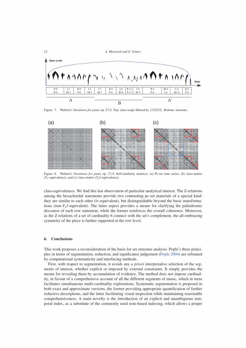
whole pattern is restated throughout the movement, evolving at different transpositional and/orinversional levels. This holds strictly in the four expositions of the series in Section A, wherethe sequence of hexachords 6-Z41, 6-Z12, 6-Z12, and 6-Z41 is presented four times. SectionA’ virtually reconstructs the same pattern. The well-known structure of the piece is shown inFigure 7 (bottom), annotated according to Cook (1987), and time aligned with the class-scape(top).

A self-similarity matrix is a simple technique for finding recurrences in time series in general,and for pattern discovery in music in particular (Foote 1999). This data structure represents thedistance of all the pairwise elements19 in the time series according to some similarity measure.The most likely recurrences are revealed by diagonals in the matrix accumulating high similarityscores. Self-similarity matrices were computed for three different descriptors over time: (a) thepc-set time series, realized in time20; (b) the class-matrix under Tn-equivalence; and (c) the class-matrix under TnI-equivalence. The self-similarity matrix computed from the pc-set time series,depicted in Figure 8(a), does not reveal any remarkable recurrence of structural relevance. Byallowing transpositional equivalence, the first two row statements at Section A appear restated atthe beginning of A’, as shown in Figure 8(b). This is possible because the re-exposed statementsare related to their counterparts in the exposition only by transposition: P-0/R-0 and I-2/RI-2 in Section A are restated as R-4/P-4 and RI-6/I-6 in Section A’. However, it fails to matchsegments as large as the last two statements of the series in the sections A and A’, since the directpresentation (R-0/P-0) is re-exposed in inverted form (I-11/RI-11), and vice versa (I-2/RI-2 asR-9/P-9). Finally, by using transpositional and inversional equivalence, in Figure 8(c), all therow statements at A are fully revealed at A’.

The prominent recurrence of a surface phenomenon, here an hexachordal iv-sonority, leadsone to question its pertinence from analytical or perceptual standpoints. As Hasty suggested,“it is the perception of musical articulations which might result from the analyses that offer atest of validity of analytical statements” (Hasty 1981, 85, footnote 2). As we have shown, theset of sonorities revealed by our method is justified by: (a) the structure of the series; (b) theharmonization of the direct and retrograde rows in hexachords; (c) the score punctuation delin-eating those hexachords; (d) the relations among the hexachordal instantiations under different

19 Usually, time frames of a multidimensional time series.20 The information conveyed by a piano roll representation, which constitutes a symbolic substitute of the chroma

features, which are extensively used for similar tasks in the audio domain (Müller 2007). Both signals do not representidentical information, although many chroma implementations actually aim to capture the ideal pc-sets.


Figure 7. Webern’s Variations for piano op. 27/I. Top: class-scape filtered by 〈332232〉. Bottom: structure.

(a) (b) (c)

Figure 8. Webern’s Variations for piano op. 27/I. Self-similarity matrices: (a) Pc-set time series, (b) class-matrix(Tn-equivalence), and (c) class-matrix (TnI-equivalence).

class-equivalences. We find this last observation of particular analytical interest. The Z-relationsamong the hexachordal statements provide two contrasting pc-set materials of a special kind:they are similar to each other (iv-equivalent), but distinguishable beyond the basic transforma-tions (non-TnI-equivalent). The latter aspect provides a means for clarifying the palindromicdiscourse of each row statement, while the former reinforces the overall coherence. Moreover,as the Z-relations of a set of cardinality 6 connect with the set’s complement, the all-embracingsymmetry of the piece is further supported at the row level.

6. Conclusions

This work proposes a reconsideration of the basis for set structure analysis. Pople’s three princi-ples in terms of segmentation, reduction, and significance judgement (Pople 2004) are reframedby computational systematicity and interfacing methods.

First, with respect to segmentation, it avoids any a priori interpretative selection of the seg-ments of interest, whether explicit or imposed by external constraints. It simply provides themeans for revealing them by accumulation of evidence. The method does not impose cardinal-ity, in favour of a comprehensive account of all the different segments of music, which in turnsfacilitates simultaneous multi-cardinality explorations. Systematic segmentation is proposed inboth exact and approximate versions, the former providing appropriate quantification of furtherreductive descriptions, and the latter facilitating visual inspection while maintaining reasonablecomprehensiveness. A main novelty is the introduction of an explicit and unambiguous tem-poral index, as a substitute of the commonly used note-based indexing, which allows a proper


description with respect to time. This segmentation level does not contribute to interpretationartefacts of any kind, as all the possible different segments are individually considered.

Second, it avoids a priori reductive classifications. Systematicity accounts for every class,computed from the actual content of every segment. This provides a neutral level of descriptionand avoids quantification at this stage, which in our opinion constitutes a premature informationsummarization. The means for focusing material of analytical relevance is relegated to the visualrepresentation domain, whereby the accumulation of similar evidence highlights potential areasof interest. Since locality in this context is understood in terms of time and time-scale, the humanvisual attention can easily grasp the most stable sections, without eliminating or obscuring minor(less represented) areas of potential interest, which can be of residual nature or not. Since noaverage is performed by computational means, it is up to the analyst’s criteria to focus on differ-ent salient features, facilitating the interaction with the data. Unlike the approach in Huovinenand Tenkanen (2007), our temporal indexing method makes possible the precise inspection ofeach individual class.

Third, it provides a means for assessing the significance of sets, through further informationreductions that can account for global properties of single pieces or collections. This includesclass-matrices and class-vectors, as well as their subset versions (subclass-matrices and subclass-vectors). In all those reductions, a strict separation of classes is guaranteed, avoiding theirremoval or fusion up to the very moment of the interpretation. Quantification accounts forthe relative temporal presence of each class in the piece, whether globally or with respect toa given reference class, which allows the qualification of details at the level of class inclusion.A useful feature of the duration-based quantification is that potential classes of analytical inter-est may be revealed by prominent occurrences, as in Webern’s example. The method providesvalues of prominence, but it is compatible with the exploration of any class, no matter how littlerepresented. By interfacing the different representations, the interactive version of the methodaims to assist dynamic explorations of the music. The massive multidimensional information,from the global to the local, is readily available and accessible for testing. The analysis loop isthus assisted by interactive filtering of information which is guaranteed to be comprehensive,precisely described, objectively quantified and intuitively visualized.

Two main shortcomings of the method, however, are derived from combining a temporal-based segmentation with descriptions in terms of sets. First, the descriptive saturation of anysegment containing the universal pc-set, inherently featured by many segments in highly chro-matic and atonal music, for which the informativeness is often limited to short time-scales.Second, the fact that many pc-sets of analytical or perceptual relevance can only be foundby inspecting individual voices and/or fragmentary polyphonic groupings,21 a kind of surfacedescription that cannot be derived from plain temporal-based segmentations. The method can beapplied to individual or combined staves, provided the availability of proper score encodings,but this comes at the price of increasing the data dimensionality. Future research may involve thedesign of systematic representations and practical mining techniques for such information.

Acknowledgements

We would like to thank the two anonymous reviewers and the editor for their very helpful corrections and suggestions.

Funding

This work was supported by the EU Seventh Framework Programme FP7/2007-2013 through PHENICX project [grantno. 601166].

21 See Perle (1991, 84–110) for a detailed discussion about the concept of simultaneity in atonal music.


Supplemental material

The interactive potential of the methods discussed in this work can be tested by our proof-of-concept multi-scale set-class analysis tool, built upon part of the MIDI toolbox (Eerola and Toiviainen 2004), and implemented as a user interface(GUI) for Matlab. The prototype can be downloaded from http://agustin-martorell.weebly.com/set-class-analysis.html.A concise user manual of the tool, including a comprehensive table of set-classes, is also available at this site.

References

Babbit, M. 1955. “Some Aspects of Twelve-Tone Composition.” The Score and I.M.A. Magazine 12 (June): 53–61.Castrén, M. 1994. “RECREL. A Similarity Measure for Set-Classes.” PhD thesis, Sibelius Academy, Helsinki.Cook, N. 1987. A Guide to Musical Analysis. London: J. M. Dent and Sons.Eerola, T., and P. Toiviainen. 2004. MIDI Toolbox: MATLAB Tools for Music Research. Jyväskylä: University of

Jyväskylä. www.jyu.fi/musica/miditoolbox/Foote, J. 1999. “Visualizing Music and Audio Using Self-Similarity.” In ACM Multimedia, edited by J. F. Buford, S. M.

Stevens, D. C. A. Bulterman, K. Jeffay and H. J. Zhang, 77–80. Orlando, FL: ACM Press.Forte, A. 1964. “A Theory of Set-Complexes for Music.” Journal of Music Theory 8 (2): 136–183.Forte, A. 1973. The Structure of Atonal Music. New Haven: Yale University Press.Hanson, H. 1960. The Harmonic Materials of Modern Music: Resources of the Tempered Scale. New York: Appleton-

Century-Crofts.Hasty, C. 1981. “Segmentation and Process in Post-Tonal Music.” Music Theory Spectrum 3 (1): 54–73.Huovinen, E., and A. Tenkanen. 2007. “Bird’s-Eye Views of the Musical Surface: Methods for Systematic Pitch-Class

Set Analysis.” Music Analysis 26 (1–2): 159–214.Lewin, D. 1959. “Re: Intervallic Relations between Two Collections of Notes.” Journal of Music Theory 3 (2): 298–301.Lewin, D. 1979. “Some New Constructs Involving Abstract Pcsets and Probabilistic Applications.” Perspectives of New

Music 18 (1–2): 433–444.Müller, M. 2007. Information Retrieval for Music and Motion. Berlin: Springer.Perle, G. 1991. Serial Composition and Atonality. Berkeley: University of California Press.Pople, G. 2004. “Modeling Musical Structure.” In Empirical Musicology: Aims, Methods, Prospects, edited by E. Clarke

and N. Cook, 127–156. New York: Oxford University Press.Rahn, J. 1980. Basic Atonal Theory. New York: Schirmer.Rive, T. N. 1969. “An Examination of Victoria’s Technique of Adaptation and Reworking in his Parody Masses – with

Particular Attention to Harmonic and Cadential Procedure.” Anuario Musical 24: 133–152.Sapp, C. S. 2005. “Visual Hierarchical Key Analysis.” Computers in Entertainment 4 (4): 1–19.Straus, J. N. 1990. Introduction to Post-Tonal Theory. Upper Saddle River, NJ: Prentice-Hall.Tufte, E. R. 2001. The Visual Display of Quantitative Information. Cheshire, CT: Graphics Press.

Hierarchical Multi-Scale Set-Class Analysis

Documents

Transcript of Hierarchical Multi-Scale Set-Class Analysis