Hierarchical Deep Reinforcement Learning For Robotics and ...
157
Hierarchical Deep Reinforcement Learning For Robotics and Data Science Sanjay Krishnan Electrical Engineering and Computer Sciences University of California at Berkeley Technical Report No. UCB/EECS-2018-101 http://www2.eecs.berkeley.edu/Pubs/TechRpts/2018/EECS-2018-101.html August 7, 2018
-
Upload
khangminh22 -
Category
Documents
-
view
2 -
download
0
Transcript of Hierarchical Deep Reinforcement Learning For Robotics and ...
Hierarchical Deep Reinforcement Learning For Robotics andData Science
Sanjay Krishnan
Electrical Engineering and Computer SciencesUniversity of California at Berkeley
Technical Report No. UCB/EECS-2018-101http://www2.eecs.berkeley.edu/Pubs/TechRpts/2018/EECS-2018-101.html
August 7, 2018

Copyright © 2018, by the author(s).All rights reserved.
Permission to make digital or hard copies of all or part of this work forpersonal or classroom use is granted without fee provided that copies arenot made or distributed for profit or commercial advantage and that copiesbear this notice and the full citation on the first page. To copy otherwise, torepublish, to post on servers or to redistribute to lists, requires prior specificpermission.
Hierarchical Deep Reinforcement Learning ForRobotics and Data Science
by Sanjay Krishnan
A dissertation submitted in partial satisfaction of the requirements for the degree of:
Doctor of Philosophy inElectrical Engineering and Computer Sciences
in theGraduate Division of the
University of California at Berkeley
Committee in charge:Kenneth GoldbergBenjamin RechtJoshua S. Bloom
Summer 2018
1
AbstractHierarchical Deep Reinforcement Learning for Robotics and Data Science
by Sanjay KrishnanDoctor of Philosophy in Electrical Engineering and Computer Sciences
Ken Goldberg, Chair
This dissertation explores learning important structural features of a Markov DecisionProcess from offline data to significantly improve the sample-efficiency, stability, and ro-bustness of solutions even with high dimensional action spaces and long time horizons. Itpresents applications to surgical robot control, data cleaning, and generating efficient exe-cution plans for relational queries. The dissertation contributes: (1) Sequential WindowedReinforcement Learning: a framework that approximates a long-horizon MDP with a se-quence of shorter term MDPs with smooth quadratic cost functions from a small numberof expert demonstrations, (2) Deep Discovery of Options: an algorithm that discovers hi-erarchical structure in the action space from observed demonstrations, (3) AlphaClean: asystem that decomposes a data cleaning task into a set of independent search problemsand uses deep q-learning to share structure across the problems, and (4) Learning QueryOptimizer: a system that observes executions of a dynamic program for SQL query opti-mization and learns a model to predict cost-to-go values to greatly speed up future searchproblems.
Contents
1 Introduction 4Background and Related Work . . . . . . . . . . . . . . . . . . . . . . . . . . . 7
The Ubiquity of Markov Decision Processes . . . . . . . . . . . . . . . . . 8Reinforcement Learning (RL) . . . . . . . . . . . . . . . . . . . . . . . . 9Imitation Learning . . . . . . . . . . . . . . . . . . . . . . . . . . . . . . 9Reinforcement Learning with Demonstrations . . . . . . . . . . . . . . . . 10
2 Deep Discovery of Deep Options: Learning Hierarchies From Data 122.1 Overview . . . . . . . . . . . . . . . . . . . . . . . . . . . . . . . . . . . 132.2 Generative Model . . . . . . . . . . . . . . . . . . . . . . . . . . . . . . . 142.3 Expectation-Gradient Inference Algorithm . . . . . . . . . . . . . . . . . . 142.4 Experiments: Imitation . . . . . . . . . . . . . . . . . . . . . . . . . . . . 202.5 Segmentation of Robotic-Assisted Surgery . . . . . . . . . . . . . . . . . . 382.6 Experiments: Reinforcement . . . . . . . . . . . . . . . . . . . . . . . . . 39
3 Sequential Windowed Inverse Reinforcement Learning: Learning Reward De-composition From Data 453.1 Transition State Clustering . . . . . . . . . . . . . . . . . . . . . . . . . . 46
TSC Simulated Experimental Evaluation . . . . . . . . . . . . . . . . . . . 50Surgical Data Experiments . . . . . . . . . . . . . . . . . . . . . . . . . . 62
3.2 SWIRL: Learning With Transition States . . . . . . . . . . . . . . . . . . . 73Reward Learning Algorithm . . . . . . . . . . . . . . . . . . . . . . . . . 75Policy Learning . . . . . . . . . . . . . . . . . . . . . . . . . . . . . . . . 76Simulated Experiments . . . . . . . . . . . . . . . . . . . . . . . . . . . . 78Physical Experiments with the da Vinci Surgical Robot . . . . . . . . . . . 87
4 Alpha Clean: Reinforcement Learning For Data Cleaning 924.1 Problem Setup . . . . . . . . . . . . . . . . . . . . . . . . . . . . . . . . . 944.2 Architecture and API . . . . . . . . . . . . . . . . . . . . . . . . . . . . . 984.3 Search Algorithm . . . . . . . . . . . . . . . . . . . . . . . . . . . . . . . 994.4 Experiments . . . . . . . . . . . . . . . . . . . . . . . . . . . . . . . . . . 103
2

CONTENTS 3
5 Reinforcement Learning For SQL Query Optimization 1135.1 Problem Setup . . . . . . . . . . . . . . . . . . . . . . . . . . . . . . . . . 1135.2 Background . . . . . . . . . . . . . . . . . . . . . . . . . . . . . . . . . . 1155.3 Learning to Optimize . . . . . . . . . . . . . . . . . . . . . . . . . . . . . 1195.4 Reduction factor learning . . . . . . . . . . . . . . . . . . . . . . . . . . . 1215.5 Optimizer Architecture . . . . . . . . . . . . . . . . . . . . . . . . . . . . 1215.6 Experiments . . . . . . . . . . . . . . . . . . . . . . . . . . . . . . . . . . 122
6 Reinforcement Learning for Surgical Tensioning 1276.1 Motivation . . . . . . . . . . . . . . . . . . . . . . . . . . . . . . . . . . . 1286.2 Physics of Multi-Dimensional Spring Systems . . . . . . . . . . . . . . . . 1286.3 Reinforcement Learning For Policy Search . . . . . . . . . . . . . . . . . . 1316.4 Approximate Solution . . . . . . . . . . . . . . . . . . . . . . . . . . . . . 1326.5 Experiments . . . . . . . . . . . . . . . . . . . . . . . . . . . . . . . . . . 134
7 Conclusion 1407.1 Challenges and Open Problems . . . . . . . . . . . . . . . . . . . . . . . . 140

Chapter 1
Introduction
Bellman’s “Principle of Optimality” and the characterization of dynamic programming isone of the most important results in computing [11]. Its importance stems from the ubiquityof Markovian decision processes (MDPs), which formalize a wide range of problems frompath planning to scheduling [49]. In the most abstract form, there is an agent who makesa sequence of decisions to effect change on a system that processes these decisions andupdates its internal state possibly non-deterministically. The process is “Markovian” in thesense that the system’s current state completely determines its future progression. As anexample of an MDP, one might have to plan a sequence of motor commands to a robotto control it to a target position. Or, one might have to schedule a sequence of clustercomputing tasks while avoiding double scheduling on a node. The solution to a MDP is adecision making policy: the optimal decision to make given any current state of the system.
Since the MDP framework is extremely general—it encompasses shortest-path graphsearch, supervised machine learning, and optimal control—the difficulty in solving a partic-ular MDP relates to what assumptions can be made about the system. A setting of interest iswhen one only assumes black-box access to the system, where no parametric model of thesystem is readily available and the agent must iteratively query the system to optimize itsdecision policy. This setting, also called reinforcement learning [121], has been the subjectof significant recent research interest. First, there are many dynamical problems for whicha closed-form analytical description of a system’s behavior is not available but one has aprogramatic approximation of how the system transitions (i.e., simulation). ReinforcementLearning (RL) allows for direct optimization of decision policies over such simulated sys-tems. Next, by virtue of the minimal assumptions, RL algorithms are extremely generaland widely applicable across many different problem settings. From a software engineer-ing perspective, this unification allows the research community to develop a small numberof optimized libraries for RL rather each domain designing/maintaining problem-specificalgorithms. Over the last few years, the combination deep neural networks and reinforce-ment learning, or Deep RL, have emerged as in robotics, AI, and machine learning as animportant area of research [85, 110, 115, 119]. Deep RL correlates features of states tosuccessful decisions using neural networks.
4
CHAPTER 1. INTRODUCTION 5
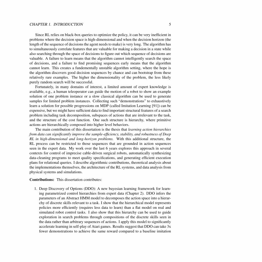
Since RL relies on black-box queries to optimize the policy, it can be very inefficient inproblems where the decision space is high-dimensional and when the decision horizon (thelength of the sequence of decisions the agent needs to make) is very long. The algorithm hasto simultaneously correlate features that are valuable for making a decision in a state whilealso searching through the space of decisions to figure out which sequence of decisions arevaluable. A failure to learn means that the algorithm cannot intelligently search the spaceof decisions, and a failure to find promising sequences early means that the algorithmcannot learn. This creates a fundementally unstable algorithm setting, where the hope isthe algorithm discovers good decision sequences by chance and can bootstrap from theserelatively rare examples. The higher the dimensionality of the problem, the less likelypurely random search will be successful.
Fortunately, in many domains of interest, a limited amount of expert knowledge isavailable, e.g., a human teleoperator can guide the motion of a robot to show an examplesolution of one problem instance or a slow classical algorithm can be used to generatesamples for limited problem instances. Collecting such “demonstrations” to exhaustivelylearn a solution for possible progressions on MDP (called Imitation Learning [91]) can beexpensive, but we might have sufficient data to find important structural features of a searchproblem including task decomposition, subspaces of actions that are irrelevant to the task,and the structure of the cost function. One such structure is hierarchy, where primitiveactions are hierarchically composed into higher level behaviors.
The main contribution of this dissertation is the thesis that learning action hierarchiesfrom data can significantly improve the sample-efficiency, stability, and robustness of DeepRL in high-dimensional and long-horizon problems. With this additional structure, theRL process can be restricted to those sequences that are grounded in action sequencesseen in the expert data. My work over the last 6 years explores this approach in severalcontexts for control of imprecise cable-driven surgical robots, automatically synthesizingdata-cleaning programs to meet quality specifications, and generating efficient executionplans for relational queries. I describe algorithmic contributions, theoretical analysis aboutthe implementations themselves, the architecture of the RL systems, and data analysis fromphysical systems and simulations.
Contributions: This dissertation contributes:
1. Deep Discovery of Options (DDO): A new bayesian learning framework for learn-ing parametrized control hierarchies from expert data (Chapter 2). DDO infers theparameters of an Abstract HMM model to decomposes the action space into a hierar-chy of discrete skills relevant to a task. I show that the hierarchical model representspolicies more efficiently (requires less data to learn) than a flat model on real andsimulated robot control tasks. I also show that this hierarchy can be used to guideexploration in search problems through compositions of the discrete skills seen inthe data rather than arbitrary sequences of actions. I apply this model to significantlyaccelerate learning in self-play of Atari games. Results suggest that DDO can take 3xfewer demonstrations to achieve the same reward compared to a baseline imitation
CHAPTER 1. INTRODUCTION 6
learning approach, and cut the sample-complexity of the RL phase by up-to an orderof magnitude.
Krishnan, Sanjay, Roy Fox, Ion Stoica, and Ken Goldberg. DDDO: Discovery ofDeep Continuous Options for Robot Learning from Demonstrations. Proceeding ofMachine Learning Research: Conference on Robot Learning. 2017.
Code for DDO is available at: https://bitbucket.org/sjyk/segment-centroid/
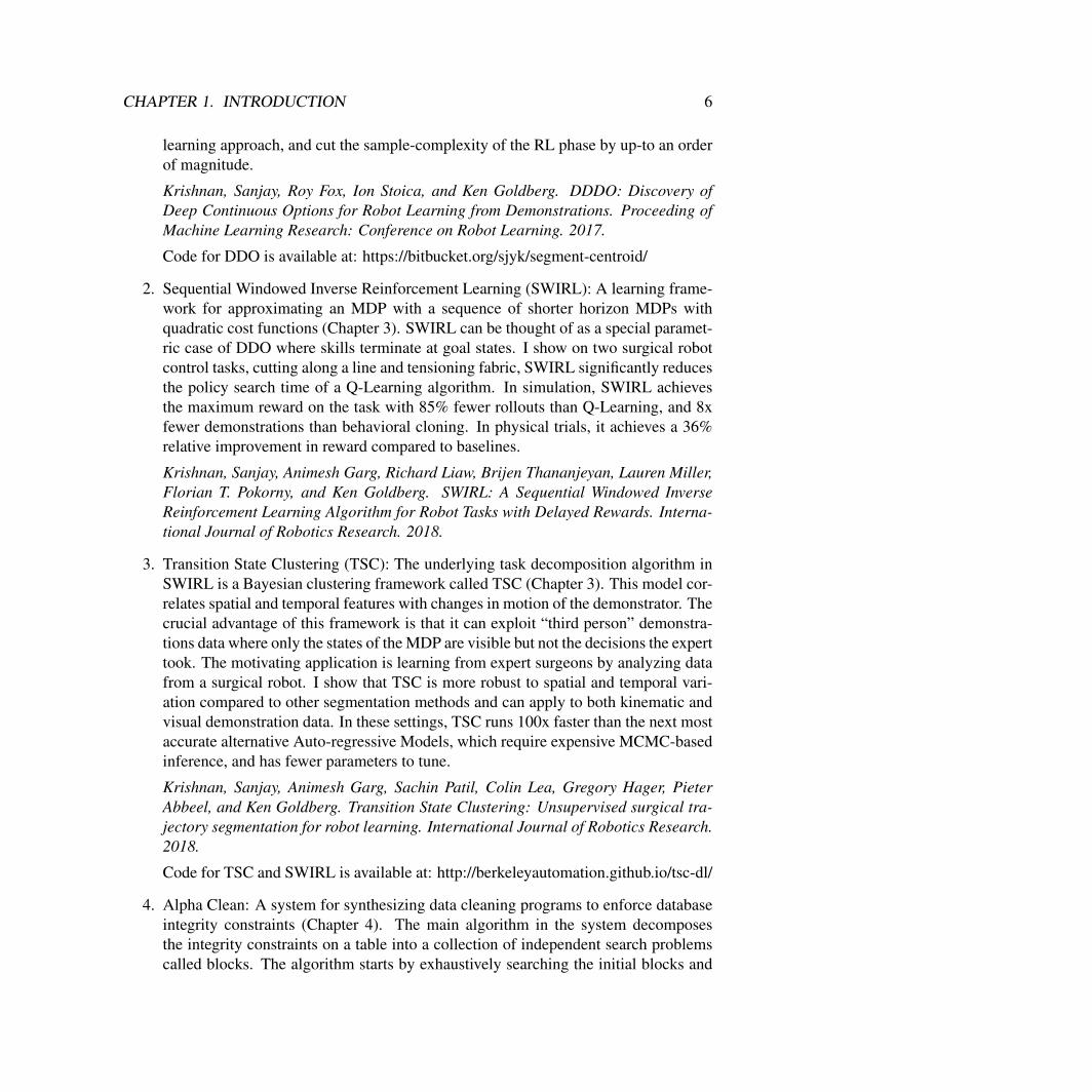
2. Sequential Windowed Inverse Reinforcement Learning (SWIRL): A learning frame-work for approximating an MDP with a sequence of shorter horizon MDPs withquadratic cost functions (Chapter 3). SWIRL can be thought of as a special paramet-ric case of DDO where skills terminate at goal states. I show on two surgical robotcontrol tasks, cutting along a line and tensioning fabric, SWIRL significantly reducesthe policy search time of a Q-Learning algorithm. In simulation, SWIRL achievesthe maximum reward on the task with 85% fewer rollouts than Q-Learning, and 8xfewer demonstrations than behavioral cloning. In physical trials, it achieves a 36%relative improvement in reward compared to baselines.
Krishnan, Sanjay, Animesh Garg, Richard Liaw, Brijen Thananjeyan, Lauren Miller,Florian T. Pokorny, and Ken Goldberg. SWIRL: A Sequential Windowed InverseReinforcement Learning Algorithm for Robot Tasks with Delayed Rewards. Interna-tional Journal of Robotics Research. 2018.
3. Transition State Clustering (TSC): The underlying task decomposition algorithm inSWIRL is a Bayesian clustering framework called TSC (Chapter 3). This model cor-relates spatial and temporal features with changes in motion of the demonstrator. Thecrucial advantage of this framework is that it can exploit “third person” demonstra-tions data where only the states of the MDP are visible but not the decisions the experttook. The motivating application is learning from expert surgeons by analyzing datafrom a surgical robot. I show that TSC is more robust to spatial and temporal vari-ation compared to other segmentation methods and can apply to both kinematic andvisual demonstration data. In these settings, TSC runs 100x faster than the next mostaccurate alternative Auto-regressive Models, which require expensive MCMC-basedinference, and has fewer parameters to tune.
Krishnan, Sanjay, Animesh Garg, Sachin Patil, Colin Lea, Gregory Hager, PieterAbbeel, and Ken Goldberg. Transition State Clustering: Unsupervised surgical tra-jectory segmentation for robot learning. International Journal of Robotics Research.2018.
Code for TSC and SWIRL is available at: http://berkeleyautomation.github.io/tsc-dl/
4. Alpha Clean: A system for synthesizing data cleaning programs to enforce databaseintegrity constraints (Chapter 4). The main algorithm in the system decomposesthe integrity constraints on a table into a collection of independent search problemscalled blocks. The algorithm starts by exhaustively searching the initial blocks and

CHAPTER 1. INTRODUCTION 7
then incrementally learns a Q-function to make the search on future increasingly pre-cise. This process leverages the fact that data cleaning is not an arbitrary constraintsatisfaction problem and most database corruption is systematic, i.e., correlated withfeatures of the data.
Krishnan, Sanjay, Eugene Wu, Michael Franklin, and Ken Goldberg. Alpha Clean:Data Cleaning with Distributed Tree Search and Learning. 2018.
Code for AlphaClean is available at: https://github.com/sjyk/alphaclean
5. A new approximate dynamic programming framework for SQL query optimization.Classical query optimizers leverage dynamic programs for optimally nesting joinqueries. This process creates a table that memoizes cost-to-go estimates of interme-diate subplans. By representing the memoization table with a neural network, theoptimizer can estimate the cost-to-go of even previously unseen plans allowing fora vast expansion of the search space. I show that this process is a form of DeepQ-Learning where the state is a query graph and the actions are contractions on thequery graph. The approach achieves plan costs within a factor of 2 of the optimalsolution on all cost models and improves on the next best heuristic by up to 3ˆ.Furthermore, it can execute up to 10,000ˆ faster than exhaustive enumeration andmore than 10ˆ faster than left/right-deep enumeration on the largest queries in thebenchmark.
Krishnan, Sanjay, Zongheng Yang, Ion Stoica, Joseph Hellerstein, and Ken Goldberg.Learning to Efficiently Enumerate Joins with Deep Reinforcement Learning. 2018.
Code for this project is available at: https://github.com/sjyk/rlqopt
6. An application of deep reinforcement learning to synthesizing surgical thin tissuetensioning policies. To improve the search time, the algorithm initializes its searchwith an analytical approximation of the equilibrium state of a FEM simulator. Theresult is a search algorithm that searches for a policy over several hundred timestepsin less than a minute of latency (Chapter 6).
Krishnan, Sanjay and Ken Goldberg. Sanjay Krishnan and Ken Goldberg. Boot-strapping Deep Reinforcement Learning of Surgical Tensioning with An AnalyticModel. C4 Surgical Workshop 2017.
Code for this project is available at: https://github.com/BerkeleyAutomation/clothsimulation
Background and Related WorkA discrete-time discounted Markov Decision Process (MDP) is described by a 6-tuplexS,A, p0, p, R, γy, where S denotes the state space, A the action space, p0 the initial statedistribution, ppst`1 | st, atq the state transition distribution, Rpst, atq P R is the reward
CHAPTER 1. INTRODUCTION 8
function, and γ P r0, 1q the discount factor. The objective of an MDP is to find a decisionpolicy, a probability distribution over actions π : S ÞÑ ∆pAq. A policy π induces thedistribution over trajectories ξ “ rps0, a0q, ps1, a1q, ..., psN , aNqs:
Pπpξq “ p0px0q
T´1ź
t“0
πpat | stqppst`1 | st, atq.
The value of a policy is its expected total discounted reward over trajectories
Vπ “ Eξ„Pπ
«
T´1ÿ
t“0
γtRpst, atq
ff
.
The objective is to find a policy in a class of allowed policies π˚ P Π to maximize thereturn:
π˚ “ arg maxπPΠ
Vπ (1)
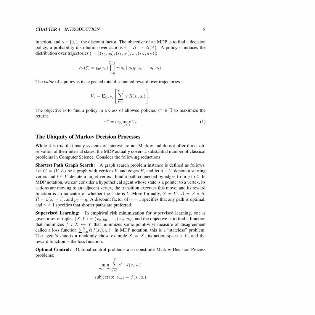
The Ubiquity of Markov Decision ProcessesWhile it is true that many systems of interest are not Markov and do not offer direct ob-servation of their internal states, the MDP actually covers a substantial number of classicalproblems in Computer Science. Consider the following reductions:
Shortest Path Graph Search: A graph search problem instance is defined as follows.Let G “ pV,Eq be a graph with vertices V and edges E, and let q P V denote a startingvertex and t P V denote a target vertex. Find a path connected by edges from q to t. InMDP notation, we can consider a hypothetical agent whose state is a pointer to a vertex, itsactions are moving to an adjacent vertex, the transition executes this move, and its rewardfunction is an indicator of whether the state is t. More formally, S “ V , A “ S ˆ S,R “ 1pst “ tq, and p0 “ q. A discount factor of γ “ 1 specifies that any path is optimal,and γ ă 1 specifies that shorter paths are preferred.
Supervised Learning: In empirical risk minimization for supervised learning, one isgiven a set of tuples pX, Y q “ px0, y0q, ..., pxN , yNq and the objective is to find a functionthat minimizes f : X ÞÑ Y that minimizes some point-wise measure of disagreementcalled a loss function
řNi“0 `pfpxiq, yiq. In MDP notation, this is a “stateless” problem.
The agent’s state is a randomly chose example S “ X , its action space is Y , and thereward function is the loss function.
Optimal Control: Optimal control problems also constitute Markov Decision Processproblems:
mina1,...,aT
Tÿ
i“1
γi ¨ Jpsi, aiq
subject to: si`1 “ fpsi, aiq
CHAPTER 1. INTRODUCTION 9
ai P A si P S s1 “ c
The problem is to select T decisions where each decision ai resides in an action space A.The decision making problem is stateful where the world has an initial state s1 and thisstate is affected by every decision the decision-making agent selects through the transitionmodel fpsi, aiq which transitions the state to another state in the set S. The objectiveis to optimize the cumulative cost of these decisions Jpsi, aiq potentially subject to anexponential discount γ that controls a bias towards short term or long term costs.
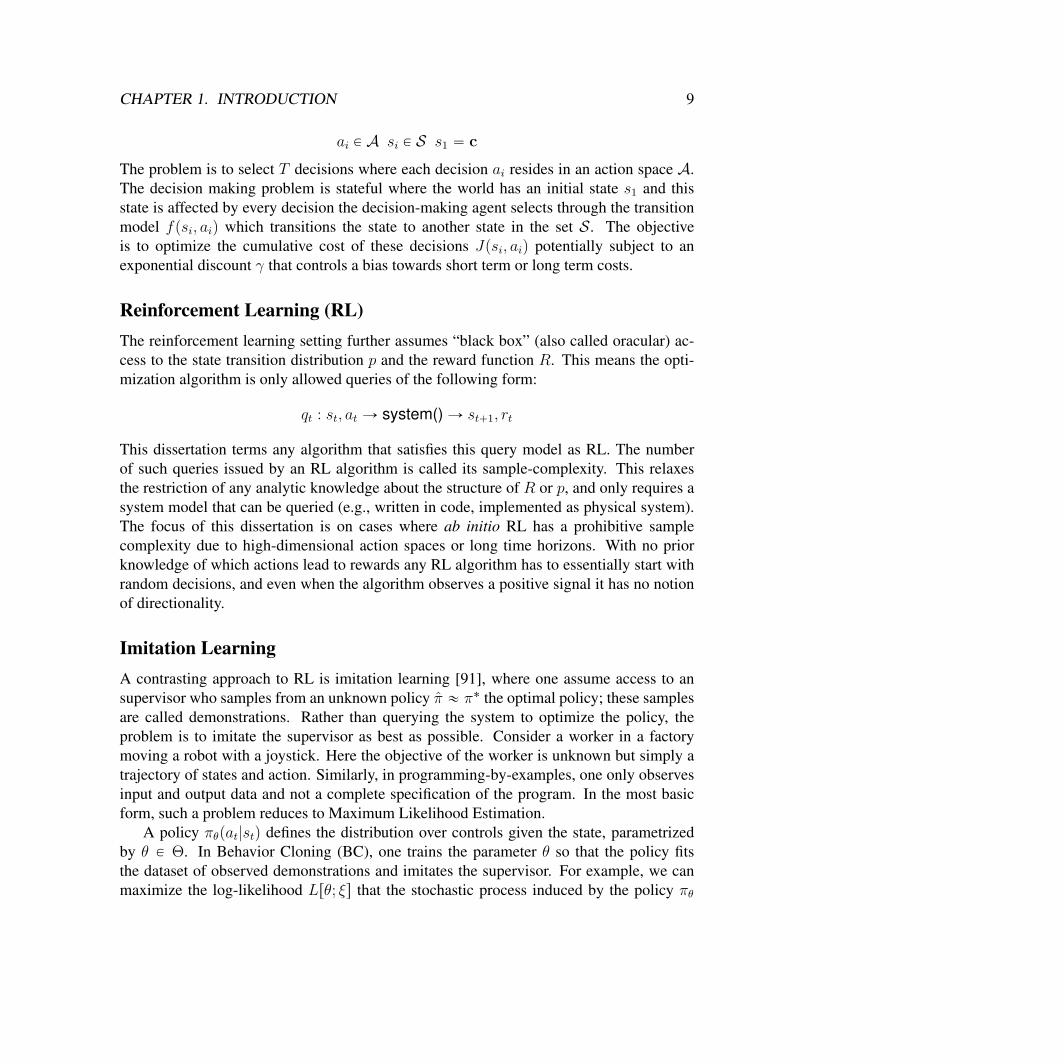
Reinforcement Learning (RL)The reinforcement learning setting further assumes “black box” (also called oracular) ac-cess to the state transition distribution p and the reward function R. This means the opti-mization algorithm is only allowed queries of the following form:
qt : st, at Ñ system() Ñ st`1, rt
This dissertation terms any algorithm that satisfies this query model as RL. The numberof such queries issued by an RL algorithm is called its sample-complexity. This relaxesthe restriction of any analytic knowledge about the structure of R or p, and only requires asystem model that can be queried (e.g., written in code, implemented as physical system).The focus of this dissertation is on cases where ab initio RL has a prohibitive samplecomplexity due to high-dimensional action spaces or long time horizons. With no priorknowledge of which actions lead to rewards any RL algorithm has to essentially start withrandom decisions, and even when the algorithm observes a positive signal it has no notionof directionality.
Imitation LearningA contrasting approach to RL is imitation learning [91], where one assume access to ansupervisor who samples from an unknown policy π « π˚ the optimal policy; these samplesare called demonstrations. Rather than querying the system to optimize the policy, theproblem is to imitate the supervisor as best as possible. Consider a worker in a factorymoving a robot with a joystick. Here the objective of the worker is unknown but simply atrajectory of states and action. Similarly, in programming-by-examples, one only observesinput and output data and not a complete specification of the program. In the most basicform, such a problem reduces to Maximum Likelihood Estimation.
A policy πθpat|stq defines the distribution over controls given the state, parametrizedby θ P Θ. In Behavior Cloning (BC), one trains the parameter θ so that the policy fitsthe dataset of observed demonstrations and imitates the supervisor. For example, we canmaximize the log-likelihood Lrθ; ξs that the stochastic process induced by the policy πθ
CHAPTER 1. INTRODUCTION 10
assigns to each demonstration trajectory ξ:
Lrθ; ξs “ log p0ps0q `
T´1ÿ
t“0
logpπθpat|stqppst`1|st, atqq.
When log πθ is parametrized by a deep neural network, we can perform stochastic gradientdescent by sampling a batch of transitions, e.g. one complete trajectory, and computing thegradient
∇θLrθ; ξs “T´1ÿ
t“0
∇θ log πθpat|stq.
Note that this method can be applied model-free, without any knowledge of the systemdynamics p.
Another approach to the imitation setting is Inverse Reinforcement Learning [3, 88,137]. This approach infers a reward function from the observed data (and possibly thesystem dynamics)–thus, reducing the problem to the original RL problem setting. [2] arguethat the reward function is often a more concise representation of task than a policy. Assuch, a concise reward function is more likely to be robust to small perturbations in thetask description. The downside is that the reward function is not useful on its own, andultimately a policy must be retrieved. In the most general case, an RL algorithm must beused to optimize for that reward function [2].
Reinforcement Learning with DemonstrationsHowever, imitation learning places a significant burden on a supervisor to exhaustivelycover the scenarios the robot may encounter during execution [74]. To address the limita-tions on either extreme of imitation and reinforcement, this dissertation proposes a hybridof the exploration and demonstration learning paradigms.
Problem 1 (Reinforcement Learning with Demonstrations) Given an MDP and a set ofdemonstration trajectories D “ tξ1, ..., ξNu from a supervisor, return a policy π˚ thatmaximizes the cumulative reward of the MDP with a reinforcement learning algorithm.
This is a problem setting that has been studied by a few recent works. In Deeply Ag-gravated [118], the expert must provide a value function in addition to actions, which ulti-mately creates an algorithm similar to Reinforcement Learning. This basic setting is alsosimilar to the problem setting consider in [96]. [117] consider a model where the randomsearch policy of the algorithm is guided by expert demonstrations. Rather than manipulat-ing the search strategy, [19] modify the “shape” the reward function to match trajectoriesseen in demonstration. This is an idea that has gotten recent traction in the robot learningcommunity [31, 48, 51].
CHAPTER 1. INTRODUCTION 11
This recent work raises a central question: what should be learned from demonstrationsto effectively bootstrap reinforcement learning? One approach is using imitation learningto learn a policy which initializes the search in RL. While this can be a very effectivestrategy, it neglects other structure that is latent in the demonstrations like are there commonsequences of actions that tend to occur or do parts of the task decompose into simpler units.In the high-dimensional setting, it is crucial to exploit such structure and this dissertationshows that different aspects of the structure such as task decomposition, action hierarchy,and action relevancy can be cast as Bayesian latent variable problems. I explore learningthis structure in detail and the impact of learning this structure on several RL problems.
Chapter 2
Deep Discovery of Deep Options:Learning Hierarchies From Data
In high-dimensional or combinatorial action spaces, the vast majority of action sequencesare irrelevant to the task at hand. Therefore, purely random exploration is likely to beprohibitively wasteful. What makes many sequential problems particularly challenging foris that all of these random action sequences are, in a sense, equally irrelevant. This meansthat there might not be any signal in the sampled data that the Q-learning algorithm canexploit. Until the agent serendipitously discovers such a sequence, no learning can occur.
In the first section of this dissertation, I explore this problem in the context of robotics,self-play in atari games, and program imitation. The basic insight is that while the space ofall action sequences AT is very large, there is often a much smaller subset of those that arepotentially relevant to typical problem instances Arelevant Ă AT . Given a small amount ofexpert information, I describe techniques for learning Arelevant from data.
How do we parametrize Arelevant? One approach is to describe the agent’s actions as acomposition higher-level behaviors called [122], each consisting of a control policy for oneregion of the state space, and a termination condition recognizing leaving that region. Thisaugmentation naturally defines a hierarchical structure of high-level meta-control policiesthat invoke lower-level options to solve sub-tasks. This leads to a “divide and conquer”relationship between the levels, where each option can specialize in short-term planningover local state features, and the meta-control policy can specialize in long-term planningover slowly changing state features. This means that any search can be restricted to theaction sequences that can be formed as a composition of skills.
Abstractions for decomposing an MDP into subtasks have been studied in the area ofhierarchical reinforcement learning (HRL) [9, 95, 122]. Early work in hierarchical con-trol demonstrated the advantages of hierarchical structures by handcrafting hierarchicalpolicies [18] and by learning them given various manual specifications: state abstrac-tions [28,47,60,61], a set of waypoints [53], low-level skills [6,50,78], a set of finite-statemeta-controllers [94], or a set of subgoals [29,122]. The key abstraction in HRL is the “op-
12
CHAPTER 2. DEEP DISCOVERY OF DEEP OPTIONS 13
tions framework” [122], which defines a hierarchy of increasingly complex meta-actions.An option represent a lower-level control primitive that can be invoked by the meta-controlpolicy at a higher-level of the hierarchy, in order to perform a certain subroutine (a usefulsequence of actions). The meta-actions invoke specialized policies rather than just takingprimitive actions.
Formally, an option h is described by a triplet
xIh, πh, ψhy,
where Ih Ă X denotes the initiation set, πhput | xtq the control policy, and ψhpstq P r0, 1sthe termination policy. When the process reaches a state s P Ih, the option h can be invokedto run the policy πh. After each action is taken and the next state s1 is reached, the option hterminates with probability ψhps1q and returns control up the hierarchy to its invoking level.The options framework enables multi-level hierarchies to be formed by allowing optionsto invoke other options. A higher-level meta-control policy is defined by augmenting itsaction space A with the setH of all lower-level options.
The options framework has been applied in robotics [63, 65, 106] and in the analysisof biological systems [15, 16, 113, 131, 135].Since then, the focus of research has shiftedtowards discovery of the hierarchical structure itself, by: trading off value with descriptionlength [125], identifying transitional states [73, 80, 82, 112, 116], inference from demon-strations [20, 27, 65, 66], iteratively expanding the set of solvable initial states [62, 63],policy gradient [77], trading off value with informational constraints [34,36,41,52], activelearning [44], or recently value-function approximation [5, 45, 107].
2.1 OverviewFirst, I describe a new learning framework for discovering a parametrized option struc-ture from a small amount of expert demonstrations. I assume that these demonstrationsare state-action demonstrations. Despite recent results in option discovery, some proposedtechniques do not generalize well to multi-level hierarchies [5, 45, 72], while others are in-efficient for learning expressive representations (e.g., options parametrized by neural net-works) [20, 27, 44, 73].
I introduce the Discovery of Deep Options (DDO), an algorithm for efficiently discov-ering deep hierarchies of deep options. DDO is a policy-gradient algorithm that discoversparametrized options from a set of demonstration trajectories (sequences of states and ac-tions) provided either by a supervisor or by roll-outs of previously learned policies. Thesedemonstrations need not be given by an optimal agent, but it is assumed that they are infor-mative of the preferred actions to take in each visited state, and are not just random walks.DDO is an inference algorithm that applies to the supervised demonstration setting.
Given a set of trajectories, the algorithm discovers a fixed, predetermined number ofoptions that are most likely to generate the observed trajectories. Since an option is repre-sented by both a control policy and a termination condition, my algorithm simultaneously
CHAPTER 2. DEEP DISCOVERY OF DEEP OPTIONS 14
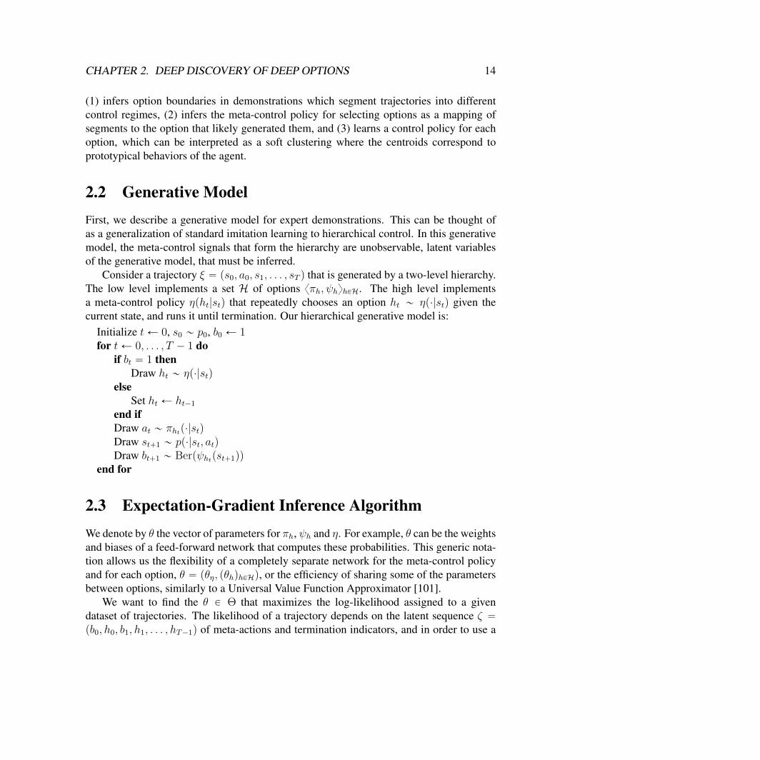
(1) infers option boundaries in demonstrations which segment trajectories into differentcontrol regimes, (2) infers the meta-control policy for selecting options as a mapping ofsegments to the option that likely generated them, and (3) learns a control policy for eachoption, which can be interpreted as a soft clustering where the centroids correspond toprototypical behaviors of the agent.
2.2 Generative ModelFirst, we describe a generative model for expert demonstrations. This can be thought ofas a generalization of standard imitation learning to hierarchical control. In this generativemodel, the meta-control signals that form the hierarchy are unobservable, latent variablesof the generative model, that must be inferred.
Consider a trajectory ξ “ ps0, a0, s1, . . . , sT q that is generated by a two-level hierarchy.The low level implements a set H of options xπh, ψhyhPH. The high level implementsa meta-control policy ηpht|stq that repeatedly chooses an option ht „ ηp¨|stq given thecurrent state, and runs it until termination. Our hierarchical generative model is:
Initialize tÐ 0, s0 „ p0, b0 Ð 1for tÐ 0, . . . , T ´ 1 do
if bt “ 1 thenDraw ht „ ηp¨|stq
elseSet ht Ð ht´1
end ifDraw at „ πhtp¨|stqDraw st`1 „ pp¨|st, atqDraw bt`1 „ Berpψhtpst`1qq
end for
2.3 Expectation-Gradient Inference AlgorithmWe denote by θ the vector of parameters for πh, ψh and η. For example, θ can be the weightsand biases of a feed-forward network that computes these probabilities. This generic nota-tion allows us the flexibility of a completely separate network for the meta-control policyand for each option, θ “ pθη, pθhqhPHq, or the efficiency of sharing some of the parametersbetween options, similarly to a Universal Value Function Approximator [101].
We want to find the θ P Θ that maximizes the log-likelihood assigned to a givendataset of trajectories. The likelihood of a trajectory depends on the latent sequence ζ “pb0, h0, b1, h1, . . . , hT´1q of meta-actions and termination indicators, and in order to use a
CHAPTER 2. DEEP DISCOVERY OF DEEP OPTIONS 15
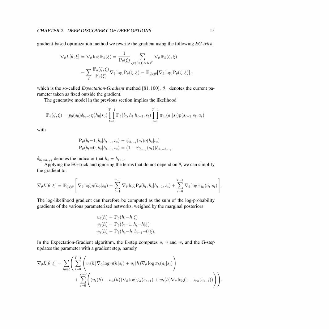
gradient-based optimization method we rewrite the gradient using the following EG-trick:
∇θLrθ; ξs “ ∇θ logPθpξq “1
Pθpξq
ÿ
ζPpt0,1uˆHqT∇θ Pθpζ, ξq
“ÿ
ζ
Pθpζ, ξq
Pθpξq∇θ logPθpζ, ξq “ Eζ|ξ;θr∇θ logPθpζ, ξqs,
which is the so-called Expectation-Gradient method [81, 100]. θ´ denotes the current pa-rameter taken as fixed outside the gradient.
The generative model in the previous section implies the likelihood
Pθpζ, ξq “ p0ps0qδb0“1ηph0|s0q
T´1ź
t“1
Pθpbt, ht|ht´1, stqT´1ź
t“0
πhtpat|stqppst`1|st, atq,
with
Pθpbt“1, ht|ht´1, stq “ ψht´1pstqηpht|stq
Pθpbt“0, ht|ht´1, stq “ p1´ ψht´1pstqqδht“ht´1 .
δht“ht`1 denotes the indicator that ht “ ht`1.Applying the EG-trick and ignoring the terms that do not depend on θ, we can simplify
the gradient to:
∇θLrθ; ξs “ Eζ|ξ;θ
«
∇θ log ηph0|s0q `
T´1ÿ
t“1
∇θ logPθpbt, ht|ht´1, stq `T´1ÿ
t“0
∇θ log πhtpat|stq
ff
.
The log-likelihood gradient can therefore be computed as the sum of the log-probabilitygradients of the various parameterized networks, weighed by the marginal posteriors
utphq “ Pθpht“h|ξq
vtphq “ Pθpbt“1, ht“h|ξq
wtphq “ Pθpht“h, bt`1“0|ξq.
In the Expectation-Gradient algorithm, the E-step computes u, v and w, and the G-stepupdates the parameter with a gradient step, namely
∇θLrθ; ξs “ÿ
hPH
˜
T´1ÿ
t“0
˜
vtphq∇θ log ηph|stq ` utphq∇θ log πhpat|stq
¸
`
T´2ÿ
t“0
˜
putphq ´ wtphqq∇θ logψhpst`1q ` wtphq∇θ logp1´ ψhpst`1qq
¸¸
.
CHAPTER 2. DEEP DISCOVERY OF DEEP OPTIONS 16
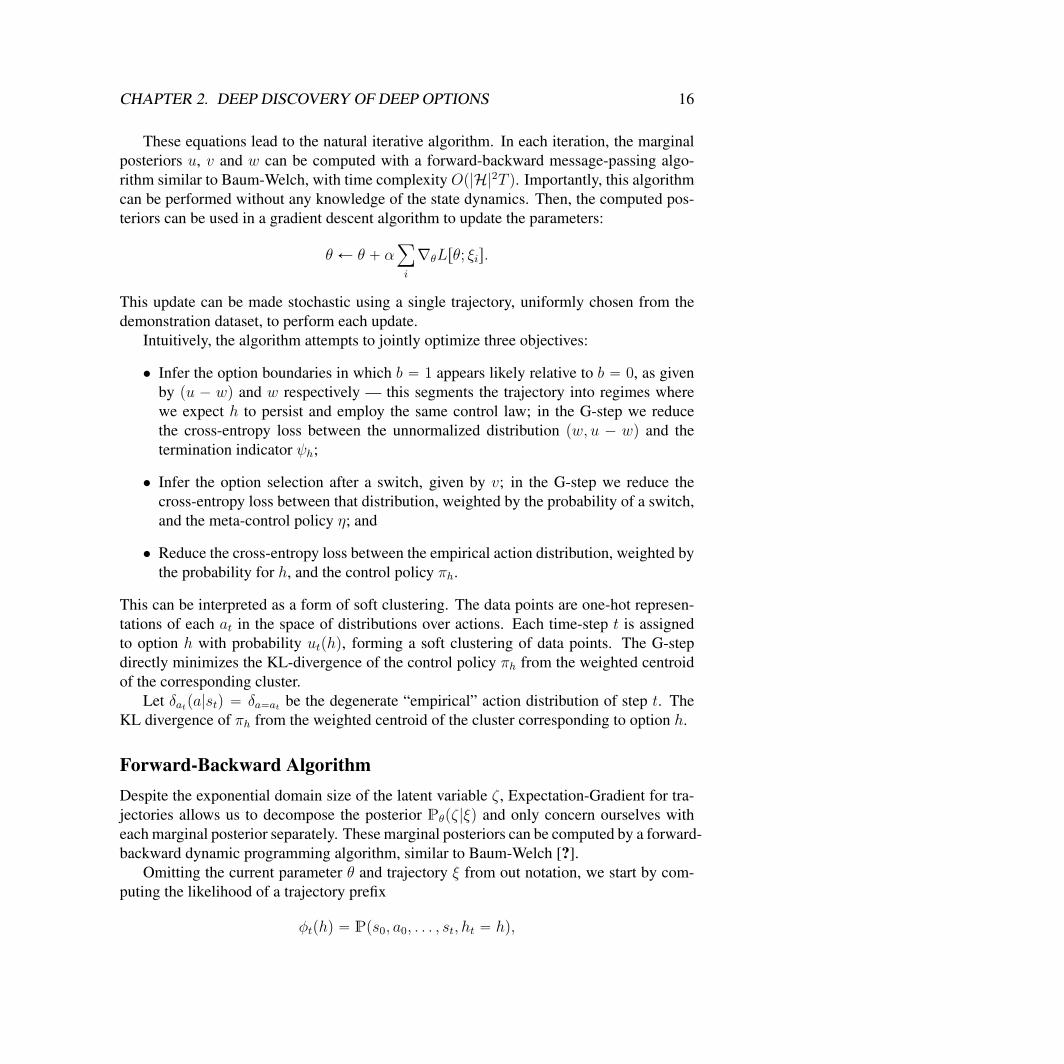
These equations lead to the natural iterative algorithm. In each iteration, the marginalposteriors u, v and w can be computed with a forward-backward message-passing algo-rithm similar to Baum-Welch, with time complexity Op|H|2T q. Importantly, this algorithmcan be performed without any knowledge of the state dynamics. Then, the computed pos-teriors can be used in a gradient descent algorithm to update the parameters:
θ Ð θ ` αÿ
i
∇θLrθ; ξis.
This update can be made stochastic using a single trajectory, uniformly chosen from thedemonstration dataset, to perform each update.
Intuitively, the algorithm attempts to jointly optimize three objectives:
• Infer the option boundaries in which b “ 1 appears likely relative to b “ 0, as givenby pu ´ wq and w respectively — this segments the trajectory into regimes wherewe expect h to persist and employ the same control law; in the G-step we reducethe cross-entropy loss between the unnormalized distribution pw, u ´ wq and thetermination indicator ψh;
• Infer the option selection after a switch, given by v; in the G-step we reduce thecross-entropy loss between that distribution, weighted by the probability of a switch,and the meta-control policy η; and
• Reduce the cross-entropy loss between the empirical action distribution, weighted bythe probability for h, and the control policy πh.
This can be interpreted as a form of soft clustering. The data points are one-hot represen-tations of each at in the space of distributions over actions. Each time-step t is assignedto option h with probability utphq, forming a soft clustering of data points. The G-stepdirectly minimizes the KL-divergence of the control policy πh from the weighted centroidof the corresponding cluster.
Let δatpa|stq “ δa“at be the degenerate “empirical” action distribution of step t. TheKL divergence of πh from the weighted centroid of the cluster corresponding to option h.
Forward-Backward AlgorithmDespite the exponential domain size of the latent variable ζ , Expectation-Gradient for tra-jectories allows us to decompose the posterior Pθpζ|ξq and only concern ourselves witheach marginal posterior separately. These marginal posteriors can be computed by a forward-backward dynamic programming algorithm, similar to Baum-Welch [?].
Omitting the current parameter θ and trajectory ξ from out notation, we start by com-puting the likelihood of a trajectory prefix
φtphq “ Pps0, a0, . . . , st, ht “ hq,

CHAPTER 2. DEEP DISCOVERY OF DEEP OPTIONS 17
using the forward recursion
φ0phq “ p0ps0qηph|s0q
φt`1ph1q “
ÿ
hPHνtphqπhpat|stqppst`1|st, atqPph
1|h, st`1q,
with
Pph1|h, st`1q “ ψhpst`1qηph1|st`1q ` p1´ ψhpst`1qqδh,h1 .
We similarly compute the likelihood of a trajectory suffix
ωtphq “ Ppat, st`1, . . . , sT |st, ht “ hq,
using the backward recursion
ωT phq “ 1
ωtphq “ πhpat|stqppst`1|st, atqÿ
h1PHPph1|h, st`1qωt`1ph
1q.
We can now compute our target likelihood using any 0 ď t ď T
Ppξq “ÿ
hPHPpξ, ht “ hq “
ÿ
hPHφtphqωtphq.
The marginal posteriors are
utphq “φtphqωtphq
Ppξq
vtphq “φtphqπhpat|stqppst`1|st, atqψhpst`1q
ř
h1PH ηph1|st`1qωt`1ph
1q
Ppξq
wtph1q “
ř
hPH φtphqπhpat|stqppst`1|st, atqψhpst`1qηph1|st`1qωt`1ph
1q
Ppξq.
Note that the constant p0ps0qśT´1
t“0 ppst`1|st, atq is cancelled out in these normalizations.This allows us to omit these terms during the forward-backward algorithm, which can thusbe applied without any knowledge of the dynamics.
Stochastic VariantWe may collect a large number of trajectories making it difficult to scale the EG algorithm.The expensive step in this algorithm is usually the forward-backward calculation, which isan Oph2T q operation. To address this problem, we can apply a stochastic variant of the EGalgorithm, which optimizes a single trajectory for each iterate:
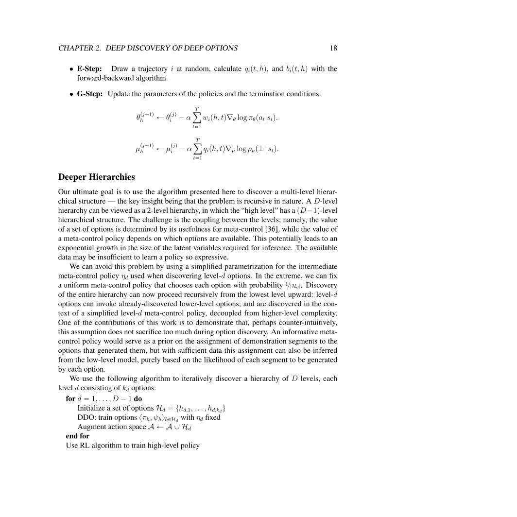
CHAPTER 2. DEEP DISCOVERY OF DEEP OPTIONS 18
• E-Step: Draw a trajectory i at random, calculate qipt, hq, and bipt, hq with theforward-backward algorithm.
• G-Step: Update the parameters of the policies and the termination conditions:
θpj`1qh Ð θ
pjqi ´ α
Tÿ
t“1
wiph, tq∇θ log πθpat|stq.
µpj`1qh Ð µ
pjqi ´ α
Tÿ
t“1
qiph, tq∇µ log ρµpK |stq.
Deeper HierarchiesOur ultimate goal is to use the algorithm presented here to discover a multi-level hierar-chical structure — the key insight being that the problem is recursive in nature. A D-levelhierarchy can be viewed as a 2-level hierarchy, in which the “high level” has a pD´1q-levelhierarchical structure. The challenge is the coupling between the levels; namely, the valueof a set of options is determined by its usefulness for meta-control [36], while the value ofa meta-control policy depends on which options are available. This potentially leads to anexponential growth in the size of the latent variables required for inference. The availabledata may be insufficient to learn a policy so expressive.
We can avoid this problem by using a simplified parametrization for the intermediatemeta-control policy ηd used when discovering level-d options. In the extreme, we can fixa uniform meta-control policy that chooses each option with probability 1{|Hd|. Discoveryof the entire hierarchy can now proceed recursively from the lowest level upward: level-doptions can invoke already-discovered lower-level options; and are discovered in the con-text of a simplified level-d meta-control policy, decoupled from higher-level complexity.One of the contributions of this work is to demonstrate that, perhaps counter-intuitively,this assumption does not sacrifice too much during option discovery. An informative meta-control policy would serve as a prior on the assignment of demonstration segments to theoptions that generated them, but with sufficient data this assignment can also be inferredfrom the low-level model, purely based on the likelihood of each segment to be generatedby each option.
We use the following algorithm to iteratively discover a hierarchy of D levels, eachlevel d consisting of kd options:
for d “ 1, . . . , D ´ 1 doInitialize a set of optionsHd “ thd,1, . . . , hd,kduDDO: train options xπh, ψhyhPHd
with ηd fixedAugment action space AÐ AYHd
end forUse RL algorithm to train high-level policy
CHAPTER 2. DEEP DISCOVERY OF DEEP OPTIONS 19
First, we approximate the high-level policy ψ, which selects policies based on the cur-rent state, with a i.i.d selection of policies based on only the previous primitive:
ψ „ Pph1|hq
This approximation is so that we do not have to simultaneously learn parameters for thehigh-level policy, while trying to optimize for the parameters of the policies and terminationconditions. Next, if we collect trajectories from multiple high-level policies, there may notexist a single high-level policy that can capture all of the trajectories. The approximationallows us to make the fewest assumptions about the structure of this policy.
Using an approximation that ψ˚ is a state-independent uniform distribution and sam-pled i.i.d, I will show the we can apply an algorithm similar to typical imitation learningapproaches that recovers the most likely parameters to estimate π˚1 , ..., π
˚k and tρ˚1 , ..., ρ
˚ku.
The basic idea is to define a probability that the current pst, atq tuple is generated by theparticular primitive h:
wph, tq “ Prh|pst, atq, τ0ăts,
and given that the current selected primitive is h probability that the current time-step istermination:
qph, tq “ PrK |pst, atq, τ0ăt, hs.
Given these probabilities, we can define an Expectation-Gradient descent over the parame-ter vector θ
θ Ð θ ` α∇θLrθ; ξs.
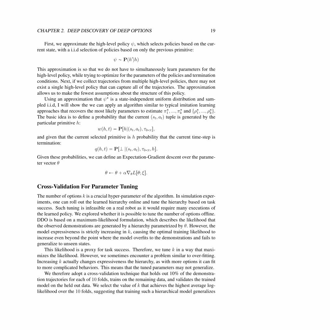
Cross-Validation For Parameter TuningThe number of options k is a crucial hyper-parameter of the algorithm. In simulation exper-iments, one can roll out the learned hierarchy online and tune the hierarchy based on tasksuccess. Such tuning is infeasible on a real robot as it would require many executions ofthe learned policy. We explored whether it is possible to tune the number of options offline.DDO is based on a maximum-likelihood formulation, which describes the likelihood thatthe observed demonstrations are generated by a hierarchy parametrized by θ. However, themodel expressiveness is strictly increasing in k, causing the optimal training likelihood toincrease even beyond the point where the model overfits to the demonstrations and fails togeneralize to unseen states.
This likelihood is a proxy for task success. Therefore, we tune k in a way that maxi-mizes the likelihood. However, we sometimes encounter a problem similar to over-fitting.Increasing k actually changes expressiveness the hierarchy, as with more options it can fitto more complicated behaviors. This means that the tuned parameters may not generalize.
We therefore adopt a cross-validation technique that holds out 10% of the demonstra-tion trajectories for each of 10 folds, trains on the remaining data, and validates the trainedmodel on the held out data. We select the value of k that achieves the highest average log-likelihood over the 10 folds, suggesting that training such a hierarchical model generalizes
CHAPTER 2. DEEP DISCOVERY OF DEEP OPTIONS 20
well. We train the final policy over the entire data. This means the tuned parameter mustwork well on a hold out set. We find empirically that the cross-validated log-likelihoodserves as a good proxy to actual task performance.
Vector Quantization For InitializationOne challenge with DDO is initialization. When real perceptual data is used, if all ofthe low-level policies initialize randomly the forward-backward estimates needed for theExpectation-Gradient will be poorly conditioned where there is an extremely low likelihoodassigned to any particular observation. The EG algorithm relies on a segment-cluster-imitate loop, where initial policy guesses are used to segment the data based on whichpolicy best explains the given time-step, then the segments are clustered, and the policiesare updated. In a continuous control space, a randomly initialized policy may not explainany of the observed data well. This means the small differences in initialization can lead tolarge changes in the learned hierarchy.
We found that a necessary pre-processing step was a variant of vector quantization,originally proposed for problems in speech recognition. We first cluster the state observa-tions using a k-means clustering and train k behavioral cloning policies for each of theclusters. We use these k policies as the initialization for the EG iterations. Unlike therandom initialization, this means that the initial low level policies will demonstrate somepreference for actions in different parts of the state-space. We set k to be the same as the kset for the number of options, and use the same optimization parameters.
2.4 Experiments: ImitationIn the first set of experiments, we evaluate DDO in its ability to represent hierarchicalcontrol policies.
Box2D Simulation: 2D Surface Pushing with Friction and GravityIn the first experiment, we simulate a 3-link robot arm in Box2D (Figure 2.1). This armconsists of three links of lengths 5 units, 5 units, and 3 units, connected by ideal revolutejoints. The arm is controlled by setting the values of the joint angular velocities 9φ1, 9φ2, 9φ3.In the environment, there is a box that lies on a flat surface with uniform friction. Theobjective is to push this box without toppling it until it rests in a randomly chosen goalposition. After this goal state is reached, the goal position is regenerated randomly. Thetask is for the robot to push the box to as many goals as possible in 2000 time-steps. Ouralgorithmic supervisor runs the RRT Connect motion planner of the Open Motion PlanningLibrary, ompl, at each time-step planning to reach the goal. Due to the geometry of theconfiguration space and the task, there are two classes of trajectories that are generated,when the goal is to the left or right of the arm.
CHAPTER 2. DEEP DISCOVERY OF DEEP OPTIONS 21
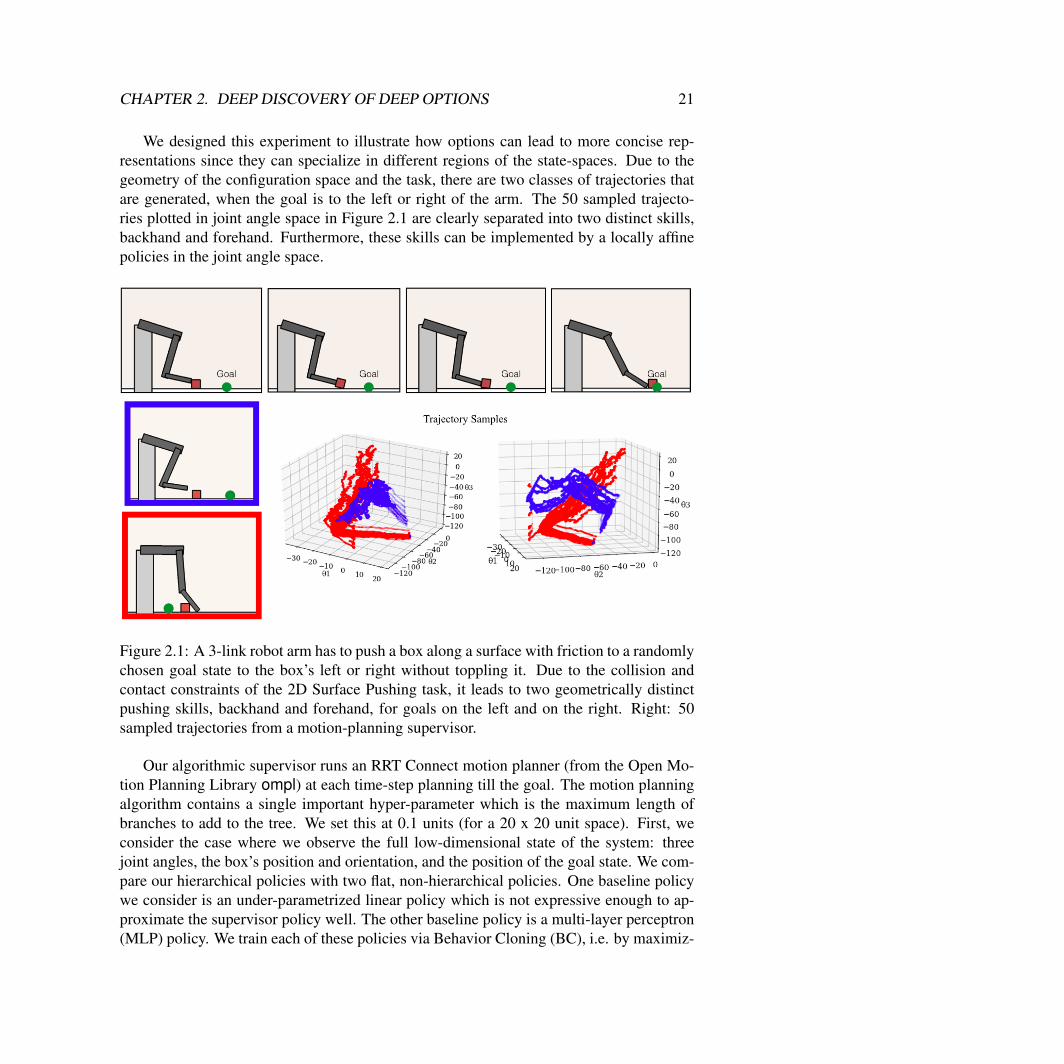
We designed this experiment to illustrate how options can lead to more concise rep-resentations since they can specialize in different regions of the state-spaces. Due to thegeometry of the configuration space and the task, there are two classes of trajectories thatare generated, when the goal is to the left or right of the arm. The 50 sampled trajecto-ries plotted in joint angle space in Figure 2.1 are clearly separated into two distinct skills,backhand and forehand. Furthermore, these skills can be implemented by a locally affinepolicies in the joint angle space.
Figure 2.1: A 3-link robot arm has to push a box along a surface with friction to a randomlychosen goal state to the box’s left or right without toppling it. Due to the collision andcontact constraints of the 2D Surface Pushing task, it leads to two geometrically distinctpushing skills, backhand and forehand, for goals on the left and on the right. Right: 50sampled trajectories from a motion-planning supervisor.
Our algorithmic supervisor runs an RRT Connect motion planner (from the Open Mo-tion Planning Library ompl) at each time-step planning till the goal. The motion planningalgorithm contains a single important hyper-parameter which is the maximum length ofbranches to add to the tree. We set this at 0.1 units (for a 20 x 20 unit space). First, weconsider the case where we observe the full low-dimensional state of the system: threejoint angles, the box’s position and orientation, and the position of the goal state. We com-pare our hierarchical policies with two flat, non-hierarchical policies. One baseline policywe consider is an under-parametrized linear policy which is not expressive enough to ap-proximate the supervisor policy well. The other baseline policy is a multi-layer perceptron(MLP) policy. We train each of these policies via Behavior Cloning (BC), i.e. by maximiz-
CHAPTER 2. DEEP DISCOVERY OF DEEP OPTIONS 22
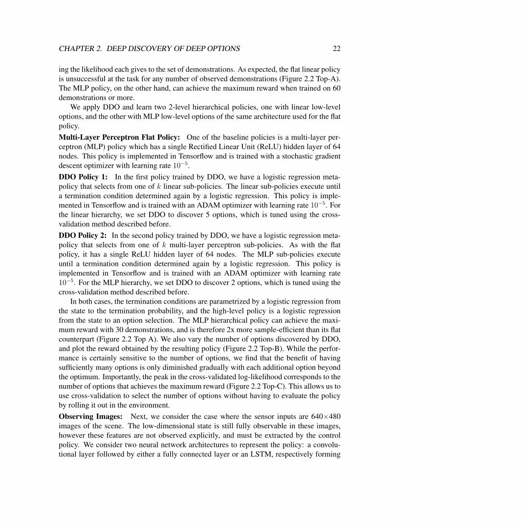
ing the likelihood each gives to the set of demonstrations. As expected, the flat linear policyis unsuccessful at the task for any number of observed demonstrations (Figure 2.2 Top-A).The MLP policy, on the other hand, can achieve the maximum reward when trained on 60demonstrations or more.
We apply DDO and learn two 2-level hierarchical policies, one with linear low-leveloptions, and the other with MLP low-level options of the same architecture used for the flatpolicy.Multi-Layer Perceptron Flat Policy: One of the baseline policies is a multi-layer per-ceptron (MLP) policy which has a single Rectified Linear Unit (ReLU) hidden layer of 64nodes. This policy is implemented in Tensorflow and is trained with a stochastic gradientdescent optimizer with learning rate 10´5.DDO Policy 1: In the first policy trained by DDO, we have a logistic regression meta-policy that selects from one of k linear sub-policies. The linear sub-policies execute untila termination condition determined again by a logistic regression. This policy is imple-mented in Tensorflow and is trained with an ADAM optimizer with learning rate 10´5. Forthe linear hierarchy, we set DDO to discover 5 options, which is tuned using the cross-validation method described before.DDO Policy 2: In the second policy trained by DDO, we have a logistic regression meta-policy that selects from one of k multi-layer perceptron sub-policies. As with the flatpolicy, it has a single ReLU hidden layer of 64 nodes. The MLP sub-policies executeuntil a termination condition determined again by a logistic regression. This policy isimplemented in Tensorflow and is trained with an ADAM optimizer with learning rate10´5. For the MLP hierarchy, we set DDO to discover 2 options, which is tuned using thecross-validation method described before.
In both cases, the termination conditions are parametrized by a logistic regression fromthe state to the termination probability, and the high-level policy is a logistic regressionfrom the state to an option selection. The MLP hierarchical policy can achieve the maxi-mum reward with 30 demonstrations, and is therefore 2x more sample-efficient than its flatcounterpart (Figure 2.2 Top A). We also vary the number of options discovered by DDO,and plot the reward obtained by the resulting policy (Figure 2.2 Top-B). While the perfor-mance is certainly sensitive to the number of options, we find that the benefit of havingsufficiently many options is only diminished gradually with each additional option beyondthe optimum. Importantly, the peak in the cross-validated log-likelihood corresponds to thenumber of options that achieves the maximum reward (Figure 2.2 Top-C). This allows us touse cross-validation to select the number of options without having to evaluate the policyby rolling it out in the environment.Observing Images: Next, we consider the case where the sensor inputs are 640ˆ480images of the scene. The low-dimensional state is still fully observable in these images,however these features are not observed explicitly, and must be extracted by the controlpolicy. We consider two neural network architectures to represent the policy: a convolu-tional layer followed by either a fully connected layer or an LSTM, respectively forming
CHAPTER 2. DEEP DISCOVERY OF DEEP OPTIONS 23
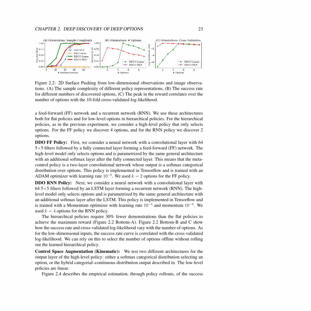
Figure 2.2: 2D Surface Pushing from low-dimensional observations and image observa-tions. (A) The sample complexity of different policy representations, (B) The success ratefor different numbers of discovered options, (C) The peak in the reward correlates over thenumber of options with the 10-fold cross-validated log-likelihood.
a feed-forward (FF) network and a recurrent network (RNN). We use these architecturesboth for flat policies and for low-level options in hierarchical policies. For the hierarchicalpolicies, as in the previous experiment, we consider a high-level policy that only selectsoptions. For the FF policy we discover 4 options, and for the RNN policy we discover 2options.DDO FF Policy: First, we consider a neural network with a convolutional layer with 645ˆ5 filters followed by a fully connected layer forming a feed-forward (FF) network. Thehigh-level model only selects options and is parametrized by the same general architecturewith an additional softmax layer after the fully connected layer. This means that the meta-control policy is a two-layer convolutional network whose output is a softmax categoricaldistribution over options. This policy is implemented in Tensorflow and is trained with anADAM optimizer with learning rate 10´5. We used k “ 2 options for the FF policy.DDO RNN Policy: Next, we consider a neural network with a convolutional layer with64 5ˆ5 filters followed by an LSTM layer forming a recurrent network (RNN). The high-level model only selects options and is parametrized by the same general architecture withan additional softmax layer after the LSTM. This policy is implemented in Tensorflow andis trained with a Momentum optimizer with learning rate 10´4 and momentum 10´3. Weused k “ 4 options for the RNN policy.
The hierarchical policies require 30% fewer demonstrations than the flat policies toachieve the maximum reward (Figure 2.2 Bottom-A). Figure 2.2 Bottom-B and C showhow the success rate and cross-validated log-likelihood vary with the number of options. Asfor the low-dimensional inputs, the success rate curve is correlated with the cross-validatedlog-likelihood. We can rely on this to select the number of options offline without rollingout the learned hierarchical policy.Control Space Augmentation (Kinematic): We test two different architectures for theoutput layer of the high-level policy: either a softmax categorical distribution selecting anoption, or the hybrid categorial–continuous distribution output described in. The low-levelpolicies are linear.
Figure 2.4 describes the empirical estimation, through policy rollouts, of the success
CHAPTER 2. DEEP DISCOVERY OF DEEP OPTIONS 24
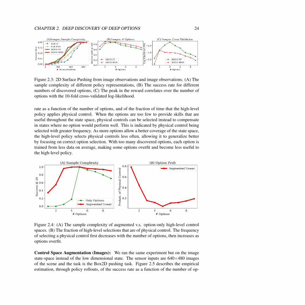
Figure 2.3: 2D Surface Pushing from image observations and image observations. (A) Thesample complexity of different policy representations, (B) The success rate for differentnumbers of discovered options, (C) The peak in the reward correlates over the number ofoptions with the 10-fold cross-validated log-likelihood.
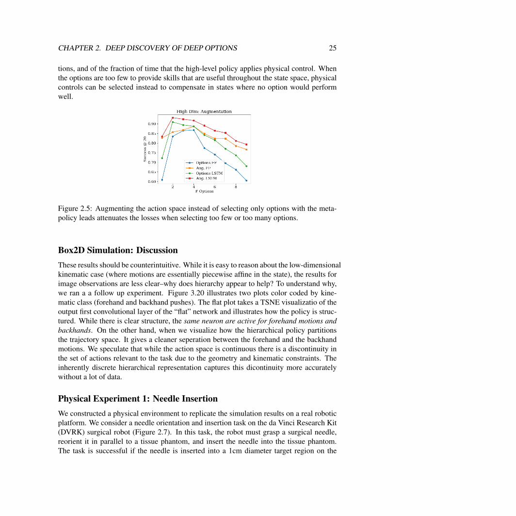
rate as a function of the number of options, and of the fraction of time that the high-levelpolicy applies physical control. When the options are too few to provide skills that areuseful throughout the state space, physical controls can be selected instead to compensatein states where no option would perform well. This is indicated by physical control beingselected with greater frequency. As more options allow a better coverage of the state space,the high-level policy selects physical controls less often, allowing it to generalize betterby focusing on correct option selection. With too many discovered options, each option istrained from less data on average, making some options overfit and become less useful tothe high-level policy.
Figure 2.4: (A) The sample complexity of augmented v.s. option-only high-level controlspaces. (B) The fraction of high-level selections that are of physical control. The frequencyof selecting a physical control first decreases with the number of options, then increases asoptions overfit.
Control Space Augmentation (Images): We ran the same experiment but on the imagestate-space instead of the low dimensional state. The sensor inputs are 640ˆ480 imagesof the scene and the task is the Box2D pushing task. Figure 2.5 describes the empiricalestimation, through policy rollouts, of the success rate as a function of the number of op-
CHAPTER 2. DEEP DISCOVERY OF DEEP OPTIONS 25
tions, and of the fraction of time that the high-level policy applies physical control. Whenthe options are too few to provide skills that are useful throughout the state space, physicalcontrols can be selected instead to compensate in states where no option would performwell.
Figure 2.5: Augmenting the action space instead of selecting only options with the meta-policy leads attenuates the losses when selecting too few or too many options.
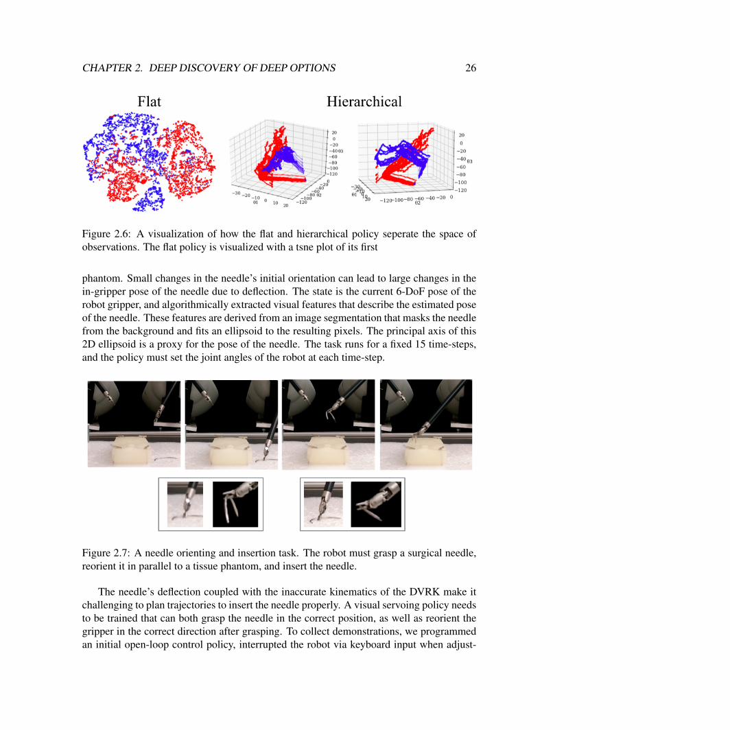
Box2D Simulation: DiscussionThese results should be counterintuitive. While it is easy to reason about the low-dimensionalkinematic case (where motions are essentially piecewise affine in the state), the results forimage observations are less clear–why does hierarchy appear to help? To understand why,we ran a a follow up experiment. Figure 3.20 illustrates two plots color coded by kine-matic class (forehand and backhand pushes). The flat plot takes a TSNE visualizatio of theoutput first convolutional layer of the “flat” network and illustrates how the policy is struc-tured. While there is clear structure, the same neuron are active for forehand motions andbackhands. On the other hand, when we visualize how the hierarchical policy partitionsthe trajectory space. It gives a cleaner seperation between the forehand and the backhandmotions. We speculate that while the action space is continuous there is a discontinuity inthe set of actions relevant to the task due to the geometry and kinematic constraints. Theinherently discrete hierarchical representation captures this dicontinuity more accuratelywithout a lot of data.
Physical Experiment 1: Needle InsertionWe constructed a physical environment to replicate the simulation results on a real roboticplatform. We consider a needle orientation and insertion task on the da Vinci Research Kit(DVRK) surgical robot (Figure 2.7). In this task, the robot must grasp a surgical needle,reorient it in parallel to a tissue phantom, and insert the needle into the tissue phantom.The task is successful if the needle is inserted into a 1cm diameter target region on the
CHAPTER 2. DEEP DISCOVERY OF DEEP OPTIONS 26
Figure 2.6: A visualization of how the flat and hierarchical policy seperate the space ofobservations. The flat policy is visualized with a tsne plot of its first
phantom. Small changes in the needle’s initial orientation can lead to large changes in thein-gripper pose of the needle due to deflection. The state is the current 6-DoF pose of therobot gripper, and algorithmically extracted visual features that describe the estimated poseof the needle. These features are derived from an image segmentation that masks the needlefrom the background and fits an ellipsoid to the resulting pixels. The principal axis of this2D ellipsoid is a proxy for the pose of the needle. The task runs for a fixed 15 time-steps,and the policy must set the joint angles of the robot at each time-step.
Figure 2.7: A needle orienting and insertion task. The robot must grasp a surgical needle,reorient it in parallel to a tissue phantom, and insert the needle.
The needle’s deflection coupled with the inaccurate kinematics of the DVRK make itchallenging to plan trajectories to insert the needle properly. A visual servoing policy needsto be trained that can both grasp the needle in the correct position, as well as reorient thegripper in the correct direction after grasping. To collect demonstrations, we programmedan initial open-loop control policy, interrupted the robot via keyboard input when adjust-
CHAPTER 2. DEEP DISCOVERY OF DEEP OPTIONS 27
ment was needed, and kinesthetically adjusted the pose of the gripper. We collected 100such demonstrations.
We evaluated the following alternatives: (1) a single flat MLP policy with continuousoutput, (2) a flat policy consisting of 15 distinct MLP networks, one for each time-step, (3)a hierarchical policy with 5 options trained with DDO. We considered a hierarchy wherethe high-level policy is a MLP with a softmax output that selects the appropriate option,and each option is parametrized by a distinct MLP with continuous outputs. DDO learns5 options, two of which roughly correspond to the visual servoing for grasping and lift-ing the needle, and the other three handle three different types of reorientation. For 100demonstrations, the hierarchical policy learned with DDO has a 45% higher log-likelihoodmeasured in cross-validation than the flat policy, and a 24% higher log-likelihood than theper-timestep policy.
Task Description: The robot must grasp a 1mm diameter surgical needle, re-orient it par-allel to a tissue phantom, and insert the needle into a tissue phantom. The task is successfulif the needle is inserted into a 1 cm diameter target region on the phantom. In this task, thestate-space is the current 6-DoF pose of the robot gripper and visual features that describethe estimated pose of the needle. These features are derived from an image segmentationthat masks the needle from the background and fits an ellipsoid to the resulting pixels. Theprincipal axis of this 2D ellipsoid is a proxy for the pose of the needle. The task runs for afixed 15 time-steps and the policy must set the joint angles of the robot at each time-step.
Robot Parameters: The challenge is that the curved needle is sensitive to the way that itis grasped. Small changes in the needle’s initial orientation can lead to large changes to thein-gripper pose of the needle due to deflection. This deflection coupled with the inaccuratekinematics of the DVRK leads to very different trajectories to insert the needle properly.
The robotic setup includes a stereo endoscope camera located 650 mm above the 10cmx 10 cm workspace. After registration, the dvrk has an RMSE kinematic error of 3.3 mm,and for reference, a gripper width of 1 cm. In some regions of the state-space this erroris even higher, with a 75% percentile error of 4.7 mm. The learning in this task couples avisual servoing policy to grasp the needle with the decision of which direction to orient thegripper after grasping.
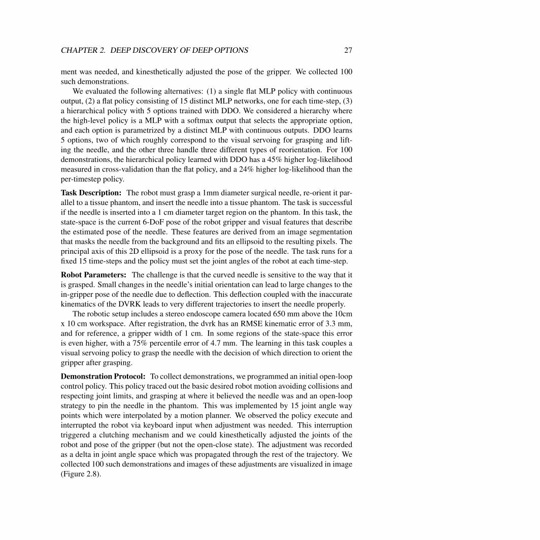
Demonstration Protocol: To collect demonstrations, we programmed an initial open-loopcontrol policy. This policy traced out the basic desired robot motion avoiding collisions andrespecting joint limits, and grasping at where it believed the needle was and an open-loopstrategy to pin the needle in the phantom. This was implemented by 15 joint angle waypoints which were interpolated by a motion planner. We observed the policy execute andinterrupted the robot via keyboard input when adjustment was needed. This interruptiontriggered a clutching mechanism and we could kinesthetically adjusted the joints of therobot and pose of the gripper (but not the open-close state). The adjustment was recordedas a delta in joint angle space which was propagated through the rest of the trajectory. Wecollected 100 such demonstrations and images of these adjustments are visualized in image(Figure 2.8).
CHAPTER 2. DEEP DISCOVERY OF DEEP OPTIONS 28
Figure 2.8: To collect demonstrations, we programmed an initial open-loop control pol-icy. We observed the policy execute and interrupted the robot via keyboard input whenadjustment was needed.
Learning the Parameters: Figure 2.9A plots the cross-validation log-likelihood as afunction of the number of demonstrations. We find that the hierarchical model has a higherlikelihood than the alternatives—meaning that it more accurately explains the observeddata and generalizes better to held out data. At some points, the relative difference is over30%. It, additionally, provides some interpretability to the learned policy. Figure 2.9Bvisualizes two representative trajectories. We color code the trajectory based on the optionactive at each state (estimated by DDO). The algorithm separates each trajectory into 3segments: needle grasping, needle lifting, and needle orienting. The two trajectories havethe same first two options but differ in the orientation step. One of the trajectories has torotate in a different direction to orient the needle before insertion.Flat Policy: One of the baseline policies is a multi-layer perceptron (MLP) policy whichhas a single ReLU hidden layer of 64 nodes. This policy is implemented in Tensorflow andis trained with an ADAM optimizer with learning rate 10´5.Per-Timestep Policy: Next, we consider a degenerate case of options where each policyexecutes for a single-timestep. We train 15 distinct multi-layer perceptron (MLP) policieseach of which has a single ReLU hidden layer of 64 nodes. Thes policies are implementedin Tensorflow and are trained with an ADAM optimizer with learning rate 10´5.DDO Policy: DDO trains a hierarchical policy with 5 options. We considered a hierarchywhere the meta policy is a multilayer perceptron with a softmax output that selects theappropriate option, and the options are parametrized by another multilayer perceptron withcontinuous outputs. Each of the MLP policies has a single ReLU hidden layer of 64 nodes.Thes policies are implemented in Tensorflow and are trained with an ADAM optimizerwith learning rate 10´5.Execution: For each of the methods, we execute ten trials and report the success rate(successfully grasped and inserted the needle in the target region), and the accuracy. The

CHAPTER 2. DEEP DISCOVERY OF DEEP OPTIONS 29
Figure 2.9: (A) We plot the cross validation likelihood of the different methods as a functionof the number of demonstrations. (B) We visualize two representative trajectories (positionand gripper orientation) color coded by the most likely option applied at that timestep. Wefind that the two trajectories have the same first two options but then differ in the final stepdue to the re-orientation of the gripper before insertion.
results are described in aggregate in the table below:
Overall Success Grasp Success Insertion Success Insertion AccuracyOpen Loop 2/10 2/10 0/0 7˘ 1 mmBehavioral Cloning 3/10 6/10 3/6 6˘ 2 mmPer Timestep 6/10 7/10 6/7 5˘ 1 mmDDO 8/10 10/10 8/10 5˘ 2 mm
We ran preliminary trials to confirm that the trained options can be executed on therobot. For each of the methods, we report the success rate in 10 trials, i.e. the fractionof trials in which the needle was successfully grasped and inserted in the target region.All of the techniques had comparable accuracy in trials where they successfully graspedand inserted the needle into the 1cm diameter target region. The algorithmic open-looppolicy only succeeded 2/10 times. Surprisingly, Behavior Cloning (BC) did not do muchbetter than the open-loop policy, succeeding only 3/10 times. Per-timestep BC was farmore successful (6/10). Finally, the hierarchical policy learned with DDO succeeded 8/10times. On 10 trials it was successful 5 times more than the direct BC approach and 2times more than the per-timestep BC approach. While not statistically significant, ourpreliminary results suggest that hierarchical imitation learning is also beneficial in terms oftask success, in addition to improving model generalization and interpretability.
CHAPTER 2. DEEP DISCOVERY OF DEEP OPTIONS 30
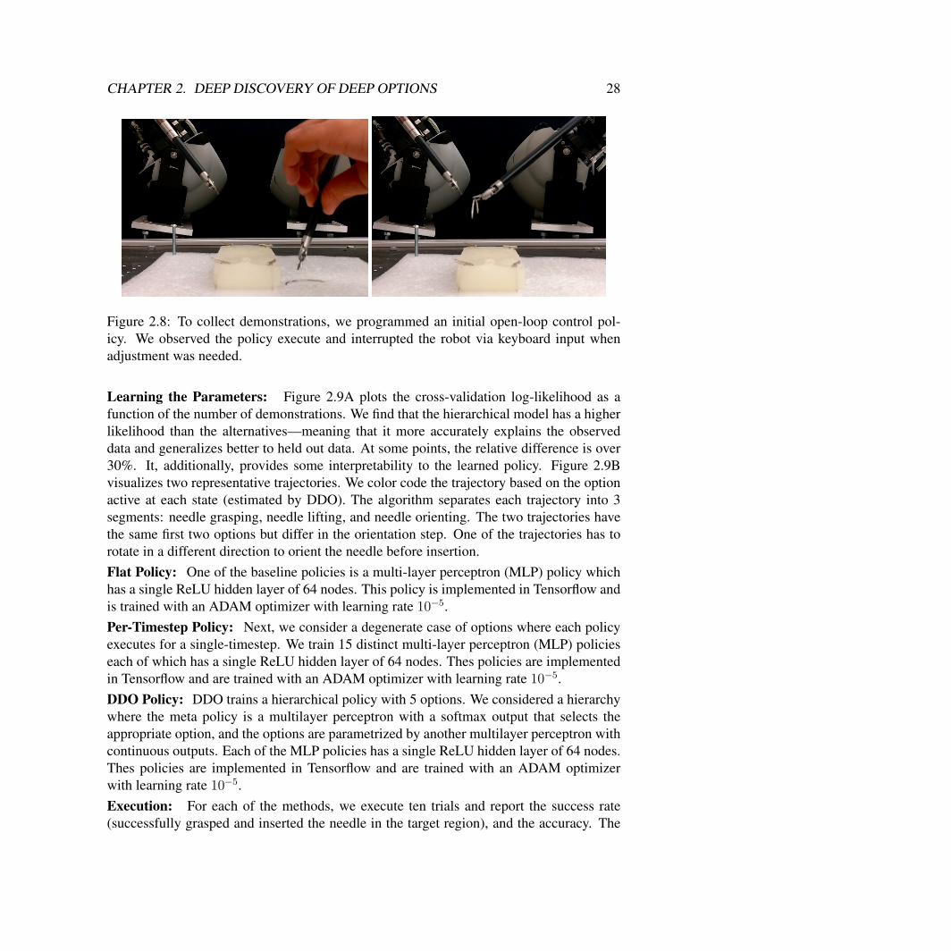
Figure 2.10: Illustration of the needle orientation and insertion task. Above are imagesillustrating the variance in the initial state, below are corresponding final states after exe-cuting DDO.
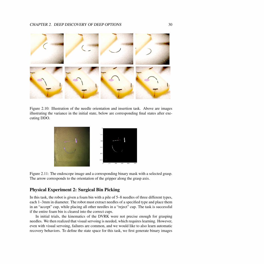
Figure 2.11: The endoscope image and a corresponding binary mask with a selected grasp.The arrow corresponds to the orientation of the gripper along the grasp axis.
Physical Experiment 2: Surgical Bin PickingIn this task, the robot is given a foam bin with a pile of 5–8 needles of three different types,each 1–3mm in diameter. The robot must extract needles of a specified type and place themin an “accept” cup, while placing all other needles in a “reject” cup. The task is successfulif the entire foam bin is cleared into the correct cups.
In initial trials, the kinematics of the DVRK were not precise enough for graspingneedles. We then realized that visual servoing is needed, which requires learning. However,even with visual servoing, failures are common, and we would like to also learn automaticrecovery behaviors. To define the state space for this task, we first generate binary images
CHAPTER 2. DEEP DISCOVERY OF DEEP OPTIONS 31
from overhead stereo images, and apply a color-based segmentation to identify the needles(the image input). Then, we use a classifier trained in advance on 40 hand-labeled imagesto identify and provide a candidate grasp point, specified by position and direction in imagespace (the grasp input). Additionally, the 6 DoF robot gripper pose and the open-closedstate of the gripper are observed (the kin input). The state space of the robot is (image,grasp, kin), and the control space is the 6 joint angles and the gripper angle.
Each sequence of grasp, lift, move, and drop operations is implemented in 10 controlsteps of joint angle positions. As in the previous task, we programmed an initial open-loopcontrol policy, interrupted the robot via keyboard input when adjustment was needed, andkinesthetically adjusted the pose of the gripper. We collected 60 such demonstrations, ineach fully clearing a pile of 3–8 needles from the bin, for a total of 450 individual grasps.
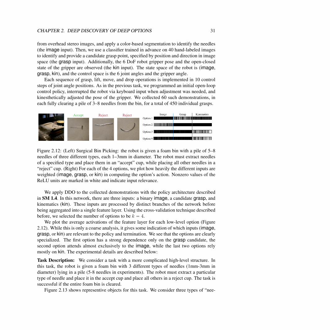
Figure 2.12: (Left) Surgical Bin Picking: the robot is given a foam bin with a pile of 5–8needles of three different types, each 1–3mm in diameter. The robot must extract needlesof a specified type and place them in an “accept” cup, while placing all other needles in a“reject” cup. (Right) For each of the 4 options, we plot how heavily the different inputs areweighted (image, grasp, or kin) in computing the option’s action. Nonzero values of theReLU units are marked in white and indicate input relevance.
We apply DDO to the collected demonstrations with the policy architecture describedin SM 1.4. In this network, there are three inputs: a binary image, a candidate grasp, andkinematics (kin). These inputs are processed by distinct branches of the network beforebeing aggregated into a single feature layer. Using the cross-validation technique describedbefore, we selected the number of options to be k “ 4.
We plot the average activations of the feature layer for each low-level option (Figure2.12). While this is only a coarse analysis, it gives some indication of which inputs (image,grasp, or kin) are relevant to the policy and termination. We see that the options are clearlyspecialized. The first option has a strong dependence only on the grasp candidate, thesecond option attends almost exclusively to the image, while the last two options relymostly on kin. The experimental details are described below:
Task Description: We consider a task with a more complicated high-level structure. Inthis task, the robot is given a foam bin with 3 different types of needles (1mm-3mm indiameter) lying in a pile (5-8 needles in experiments). The robot must extract a particulartype of needle and place it in the accept cup and place all others in a reject cup. The task issuccessful if the entire foam bin is cleared.
Figure 2.13 shows representive objects for this task. We consider three types of “nee-

CHAPTER 2. DEEP DISCOVERY OF DEEP OPTIONS 32
dles”: dissection pins, suturing needles, and wires. Dissection pins are placed in the acceptcup and the other two are placed in the reject cup.
Robot and State-Space Parameters: As in the previous task, the task requires learningbecause the kinematics of the dvrk are such that the precision needed for grasping needlesrequires visual servoing. However, even with visual servoing, failures are common due tothe pile (grasps of 2, 3, 4 objects). We would like to automatically learn recovery behaviors.In our robotic setup, there is an overhead endoscopic stereo camera, and it is located 650mmabove the workspace.
To define the state-space for this task, we first generate binary images from the stereoimages and apply a color-based segmentation to identify the needles (we call this featureimage). Then, we use a classifier derived from 40 hand-labeled images to identify possiblegrasp points to sample a candidate grasp ( left pixel value, right pixel value, and direction)(we call this feature grasp). These features are visualized in Figure 2.11. Additionally,there is the 6 DoF robot gripper pose and the open-close state of the gripper (we call thisfeature kin). The state-space of the robot is (kin, image, grasp), and the action space forthe robot is 6 joint angles and the gripper angle. Each grasp, lift, move, and drop operationconsists of 10 time steps of joint angle positions. The motion between the joint angles isperformed using a SLURP-based motion planner.
Figure 2.13: There are two bins, one accept and one reject bin. In the accept bin, we placedissection pins and place the suturing needles and the wires in the other.
Demonstration Protocol: As in the previous task, to collect demonstrations, we start witha hard-coded open-loop policy. We roll this policy out and interrupt the policy when we an-ticipate a failure. Then, we kinesthetically adjust the pose of the dvrk and it continues. Wecollected 60 such demonstrations of fully clearing the bin filled with 3 to 8 needles each–corresponding to 450 individual grasps. We also introduced a key that allows the robot tostop in place and drop it current grasped needle. Recovery behaviors were triggered whenthe robot grasps no objects or more than one object. Due to the kinesthetic corrections, a
CHAPTER 2. DEEP DISCOVERY OF DEEP OPTIONS 33
very high percentage of the attempted grasps (94%) grasped at least one object. Of the suc-cessful grasps, when 5 objects are in the pile 32% grasps picked up 2 objects, 14% pickedup 3 objects, and 0.5% picked up 4. In recovery, the gripper is opened and the epsiode endsleaving the arm in place. The next grasping trial starts from this point.
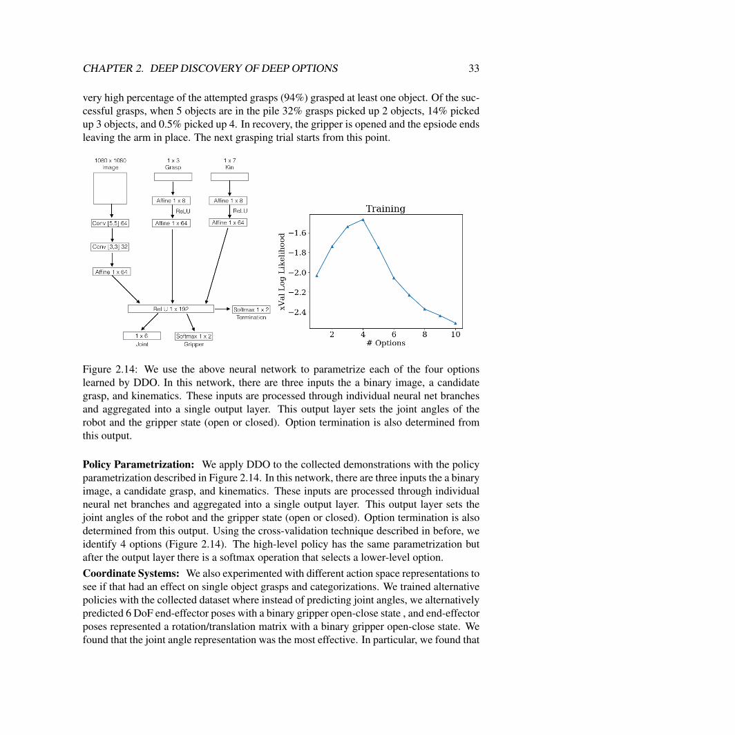
Figure 2.14: We use the above neural network to parametrize each of the four optionslearned by DDO. In this network, there are three inputs the a binary image, a candidategrasp, and kinematics. These inputs are processed through individual neural net branchesand aggregated into a single output layer. This output layer sets the joint angles of therobot and the gripper state (open or closed). Option termination is also determined fromthis output.
Policy Parametrization: We apply DDO to the collected demonstrations with the policyparametrization described in Figure 2.14. In this network, there are three inputs the a binaryimage, a candidate grasp, and kinematics. These inputs are processed through individualneural net branches and aggregated into a single output layer. This output layer sets thejoint angles of the robot and the gripper state (open or closed). Option termination is alsodetermined from this output. Using the cross-validation technique described in before, weidentify 4 options (Figure 2.14). The high-level policy has the same parametrization butafter the output layer there is a softmax operation that selects a lower-level option.Coordinate Systems: We also experimented with different action space representations tosee if that had an effect on single object grasps and categorizations. We trained alternativepolicies with the collected dataset where instead of predicting joint angles, we alternativelypredicted 6 DoF end-effector poses with a binary gripper open-close state , and end-effectorposes represented a rotation/translation matrix with a binary gripper open-close state. Wefound that the joint angle representation was the most effective. In particular, we found that
CHAPTER 2. DEEP DISCOVERY OF DEEP OPTIONS 34
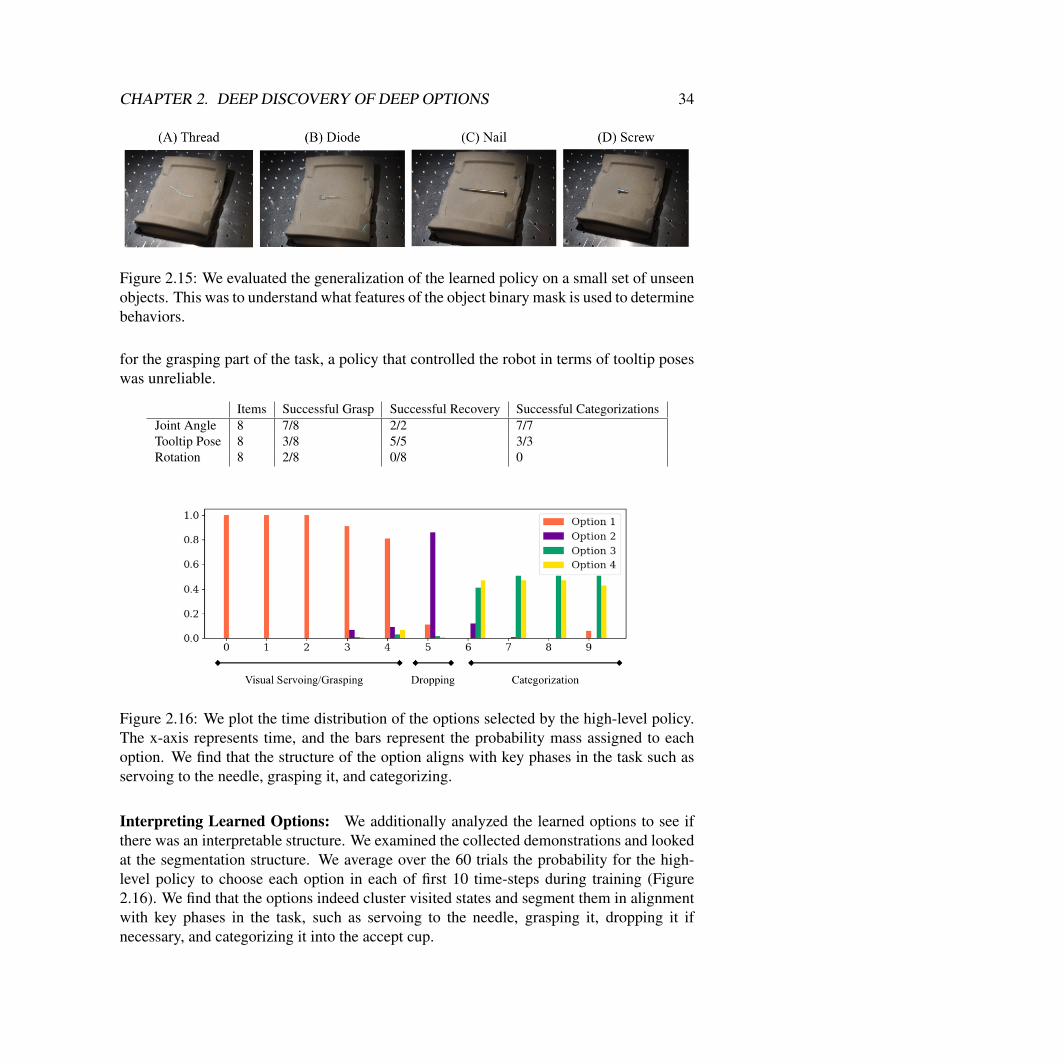
Figure 2.15: We evaluated the generalization of the learned policy on a small set of unseenobjects. This was to understand what features of the object binary mask is used to determinebehaviors.
for the grasping part of the task, a policy that controlled the robot in terms of tooltip poseswas unreliable.
Items Successful Grasp Successful Recovery Successful CategorizationsJoint Angle 8 7/8 2/2 7/7Tooltip Pose 8 3/8 5/5 3/3Rotation 8 2/8 0/8 0
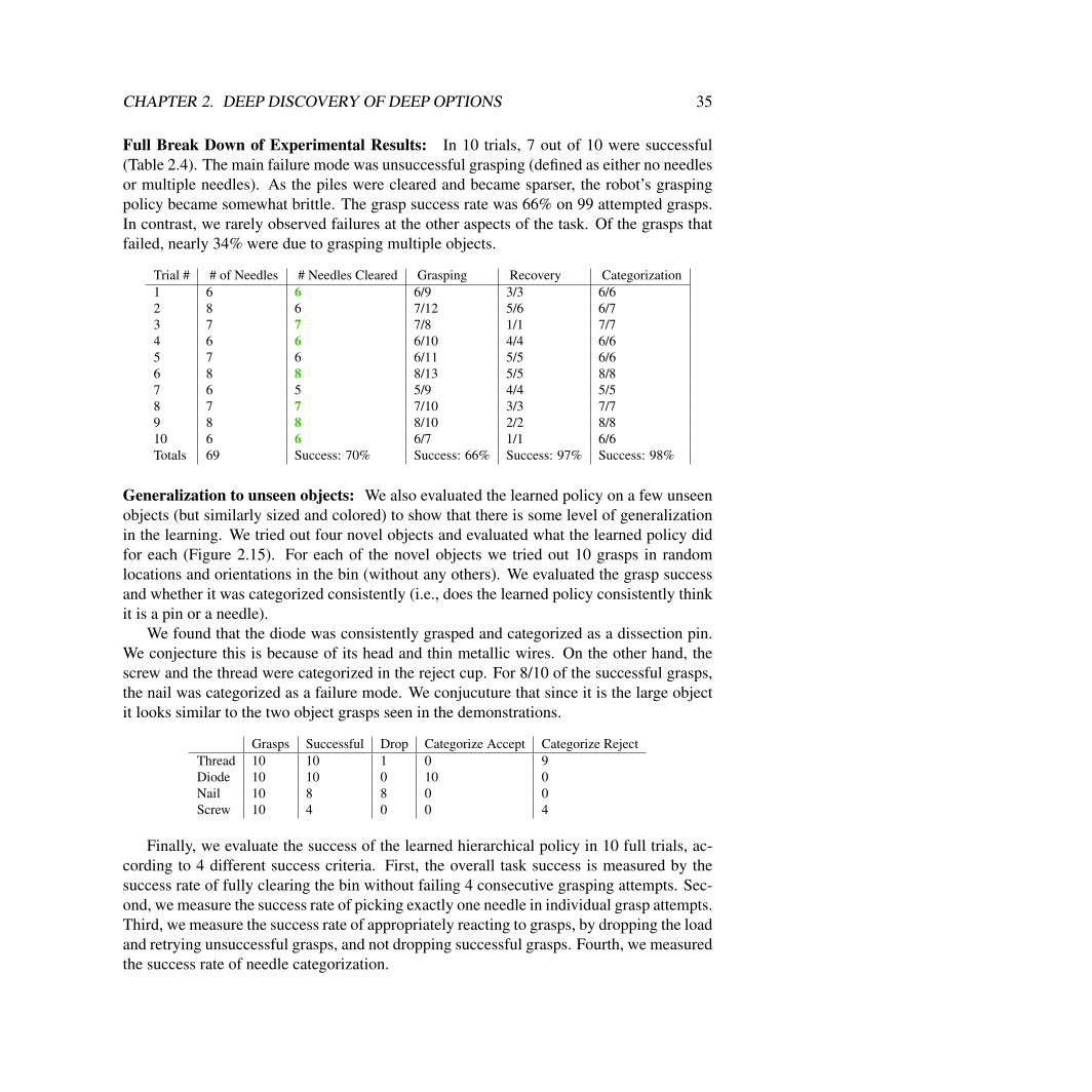
Figure 2.16: We plot the time distribution of the options selected by the high-level policy.The x-axis represents time, and the bars represent the probability mass assigned to eachoption. We find that the structure of the option aligns with key phases in the task such asservoing to the needle, grasping it, and categorizing.
Interpreting Learned Options: We additionally analyzed the learned options to see ifthere was an interpretable structure. We examined the collected demonstrations and lookedat the segmentation structure. We average over the 60 trials the probability for the high-level policy to choose each option in each of first 10 time-steps during training (Figure2.16). We find that the options indeed cluster visited states and segment them in alignmentwith key phases in the task, such as servoing to the needle, grasping it, dropping it ifnecessary, and categorizing it into the accept cup.
CHAPTER 2. DEEP DISCOVERY OF DEEP OPTIONS 35
Full Break Down of Experimental Results: In 10 trials, 7 out of 10 were successful(Table 2.4). The main failure mode was unsuccessful grasping (defined as either no needlesor multiple needles). As the piles were cleared and became sparser, the robot’s graspingpolicy became somewhat brittle. The grasp success rate was 66% on 99 attempted grasps.In contrast, we rarely observed failures at the other aspects of the task. Of the grasps thatfailed, nearly 34% were due to grasping multiple objects.
Trial # # of Needles # Needles Cleared Grasping Recovery Categorization1 6 6 6/9 3/3 6/62 8 6 7/12 5/6 6/73 7 7 7/8 1/1 7/74 6 6 6/10 4/4 6/65 7 6 6/11 5/5 6/66 8 8 8/13 5/5 8/87 6 5 5/9 4/4 5/58 7 7 7/10 3/3 7/79 8 8 8/10 2/2 8/810 6 6 6/7 1/1 6/6Totals 69 Success: 70% Success: 66% Success: 97% Success: 98%
Generalization to unseen objects: We also evaluated the learned policy on a few unseenobjects (but similarly sized and colored) to show that there is some level of generalizationin the learning. We tried out four novel objects and evaluated what the learned policy didfor each (Figure 2.15). For each of the novel objects we tried out 10 grasps in randomlocations and orientations in the bin (without any others). We evaluated the grasp successand whether it was categorized consistently (i.e., does the learned policy consistently thinkit is a pin or a needle).
We found that the diode was consistently grasped and categorized as a dissection pin.We conjecture this is because of its head and thin metallic wires. On the other hand, thescrew and the thread were categorized in the reject cup. For 8/10 of the successful grasps,the nail was categorized as a failure mode. We conjucuture that since it is the large objectit looks similar to the two object grasps seen in the demonstrations.
Grasps Successful Drop Categorize Accept Categorize RejectThread 10 10 1 0 9Diode 10 10 0 10 0Nail 10 8 8 0 0Screw 10 4 0 0 4
Finally, we evaluate the success of the learned hierarchical policy in 10 full trials, ac-cording to 4 different success criteria. First, the overall task success is measured by thesuccess rate of fully clearing the bin without failing 4 consecutive grasping attempts. Sec-ond, we measure the success rate of picking exactly one needle in individual grasp attempts.Third, we measure the success rate of appropriately reacting to grasps, by dropping the loadand retrying unsuccessful grasps, and not dropping successful grasps. Fourth, we measuredthe success rate of needle categorization.
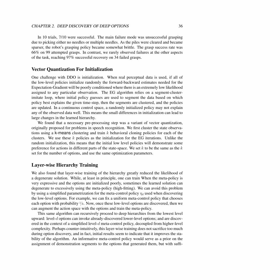
CHAPTER 2. DEEP DISCOVERY OF DEEP OPTIONS 36
In 10 trials, 7/10 were successful. The main failure mode was unsuccessful graspingdue to picking either no needles or multiple needles. As the piles were cleared and becamesparser, the robot’s grasping policy became somewhat brittle. The grasp success rate was66% on 99 attempted grasps. In contrast, we rarely observed failures at the other aspectsof the task, reaching 97% successful recovery on 34 failed grasps.
Vector Quantization For InitializationOne challenge with DDO is initialization. When real perceptual data is used, if all ofthe low-level policies initialize randomly the forward-backward estimates needed for theExpectation-Gradient will be poorly conditioned where there is an extremely low likelihoodassigned to any particular observation. The EG algorithm relies on a segment-cluster-imitate loop, where initial policy guesses are used to segment the data based on whichpolicy best explains the given time-step, then the segments are clustered, and the policiesare updated. In a continuous control space, a randomly initialized policy may not explainany of the observed data well. This means the small differences in initialization can lead tolarge changes in the learned hierarchy.
We found that a necessary pre-processing step was a variant of vector quantization,originally proposed for problems in speech recognition. We first cluster the state observa-tions using a k-means clustering and train k behavioral cloning policies for each of theclusters. We use these k policies as the initialization for the EG iterations. Unlike therandom initialization, this means that the initial low level policies will demonstrate somepreference for actions in different parts of the state-space. We set k to be the same as the kset for the number of options, and use the same optimization parameters.
Layer-wise Hierarchy TrainingWe also found that layer-wise training of the hierarchy greatly reduced the likelihood ofa degenerate solution. While, at least in principle, one can train When the meta-policy isvery expressive and the options are initialized poorly, sometimes the learned solution candegenerate to excessively using the meta-policy (high-fitting). We can avoid this problemby using a simplified parametrization for the meta-control policy ηd used when discoveringthe low-level options. For example, we can fix a uniform meta-control policy that chooseseach option with probability 1{k. Now, once these low-level options are discovered, then wecan augment the action space with the options and train the meta-policy.
This same algorithm can recursively proceed to deep hierarchies from the lowest levelupward: level-d options can invoke already-discovered lower-level options; and are discov-ered in the context of a simplified level-d meta-control policy, decoupled from higher-levelcomplexity. Perhaps counter-intuitively, this layer-wise training does not sacrifice too muchduring option discovery, and in fact, initial results seem to indicate that it improves the sta-bility of the algorithm. An informative meta-control policy would serve as a prior on theassignment of demonstration segments to the options that generated them, but with suffi-
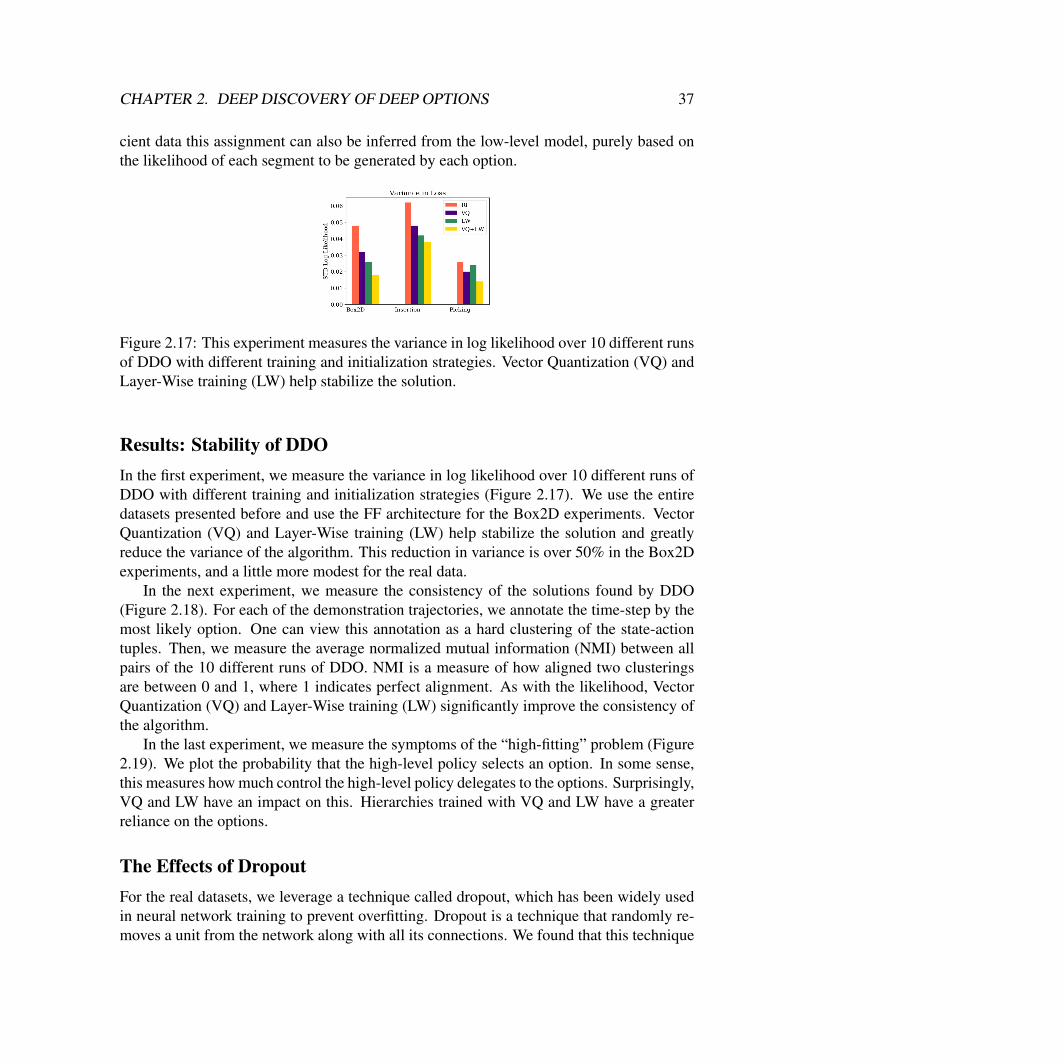
CHAPTER 2. DEEP DISCOVERY OF DEEP OPTIONS 37
cient data this assignment can also be inferred from the low-level model, purely based onthe likelihood of each segment to be generated by each option.
Figure 2.17: This experiment measures the variance in log likelihood over 10 different runsof DDO with different training and initialization strategies. Vector Quantization (VQ) andLayer-Wise training (LW) help stabilize the solution.
Results: Stability of DDOIn the first experiment, we measure the variance in log likelihood over 10 different runs ofDDO with different training and initialization strategies (Figure 2.17). We use the entiredatasets presented before and use the FF architecture for the Box2D experiments. VectorQuantization (VQ) and Layer-Wise training (LW) help stabilize the solution and greatlyreduce the variance of the algorithm. This reduction in variance is over 50% in the Box2Dexperiments, and a little more modest for the real data.
In the next experiment, we measure the consistency of the solutions found by DDO(Figure 2.18). For each of the demonstration trajectories, we annotate the time-step by themost likely option. One can view this annotation as a hard clustering of the state-actiontuples. Then, we measure the average normalized mutual information (NMI) between allpairs of the 10 different runs of DDO. NMI is a measure of how aligned two clusteringsare between 0 and 1, where 1 indicates perfect alignment. As with the likelihood, VectorQuantization (VQ) and Layer-Wise training (LW) significantly improve the consistency ofthe algorithm.
In the last experiment, we measure the symptoms of the “high-fitting” problem (Figure2.19). We plot the probability that the high-level policy selects an option. In some sense,this measures how much control the high-level policy delegates to the options. Surprisingly,VQ and LW have an impact on this. Hierarchies trained with VQ and LW have a greaterreliance on the options.
The Effects of DropoutFor the real datasets, we leverage a technique called dropout, which has been widely usedin neural network training to prevent overfitting. Dropout is a technique that randomly re-moves a unit from the network along with all its connections. We found that this technique

CHAPTER 2. DEEP DISCOVERY OF DEEP OPTIONS 38
Figure 2.18: We measure the average normalized mutual information between multipleruns of DDO. This measures the consistency of the solutions across intializations.
Figure 2.19: We measure probability that an option is selected by the high-level policy.
improved performance when the datasets were small. We set the dropout parameter to 0.5and measured the performance on a hold out set. We ran an experiment on the needle inser-tion task dataset, where we measured the cross-validation accuracy on held out data withand without dropout (Figure 2.20). Dropout seems to have a substantial effect on improvingcross-validation accuracy on a hold out set.
2.5 Segmentation of Robotic-Assisted SurgeryIn this section, we illustrate the wide applicability of the DDO framework by applying it tohuman demonstrations in a robotic domain. We apply DDO to long robotic trajectories (e.g.3 minutes) demonstrating an intricate task, and discover options for useful subtasks, as wellas segmentation of the demonstrations into semantic units. The JIGSAWS dataset consists
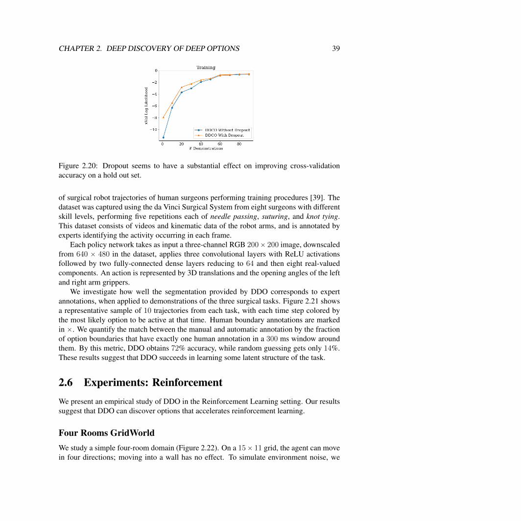
CHAPTER 2. DEEP DISCOVERY OF DEEP OPTIONS 39
Figure 2.20: Dropout seems to have a substantial effect on improving cross-validationaccuracy on a hold out set.
of surgical robot trajectories of human surgeons performing training procedures [39]. Thedataset was captured using the da Vinci Surgical System from eight surgeons with differentskill levels, performing five repetitions each of needle passing, suturing, and knot tying.This dataset consists of videos and kinematic data of the robot arms, and is annotated byexperts identifying the activity occurring in each frame.
Each policy network takes as input a three-channel RGB 200ˆ 200 image, downscaledfrom 640 ˆ 480 in the dataset, applies three convolutional layers with ReLU activationsfollowed by two fully-connected dense layers reducing to 64 and then eight real-valuedcomponents. An action is represented by 3D translations and the opening angles of the leftand right arm grippers.
We investigate how well the segmentation provided by DDO corresponds to expertannotations, when applied to demonstrations of the three surgical tasks. Figure 2.21 showsa representative sample of 10 trajectories from each task, with each time step colored bythe most likely option to be active at that time. Human boundary annotations are markedin ˆ. We quantify the match between the manual and automatic annotation by the fractionof option boundaries that have exactly one human annotation in a 300 ms window aroundthem. By this metric, DDO obtains 72% accuracy, while random guessing gets only 14%.These results suggest that DDO succeeds in learning some latent structure of the task.
2.6 Experiments: ReinforcementWe present an empirical study of DDO in the Reinforcement Learning setting. Our resultssuggest that DDO can discover options that accelerates reinforcement learning.
Four Rooms GridWorldWe study a simple four-room domain (Figure 2.22). On a 15ˆ 11 grid, the agent can movein four directions; moving into a wall has no effect. To simulate environment noise, we
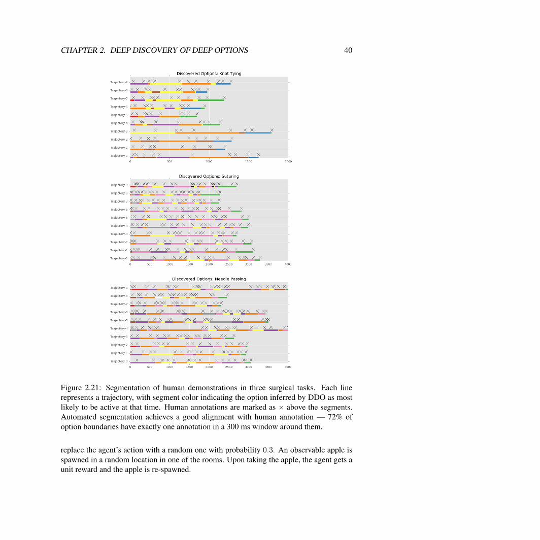
CHAPTER 2. DEEP DISCOVERY OF DEEP OPTIONS 40
Figure 2.21: Segmentation of human demonstrations in three surgical tasks. Each linerepresents a trajectory, with segment color indicating the option inferred by DDO as mostlikely to be active at that time. Human annotations are marked as ˆ above the segments.Automated segmentation achieves a good alignment with human annotation — 72% ofoption boundaries have exactly one annotation in a 300 ms window around them.
replace the agent’s action with a random one with probability 0.3. An observable apple isspawned in a random location in one of the rooms. Upon taking the apple, the agent gets aunit reward and the apple is re-spawned.
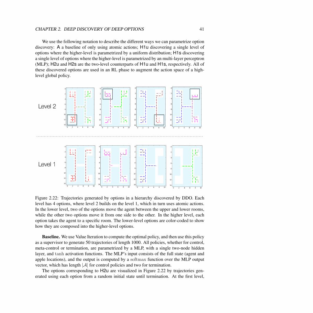
CHAPTER 2. DEEP DISCOVERY OF DEEP OPTIONS 41
We use the following notation to describe the different ways we can parametrize optiondiscovery: A a baseline of only using atomic actions; H1u discovering a single level ofoptions where the higher-level is parametrized by a uniform distribution; H1s discoveringa single level of options where the higher-level is parametrized by an multi-layer perceptron(MLP); H2u and H2s are the two-level counterparts of H1u and H1s, respectively. All ofthese discovered options are used in an RL phase to augment the action space of a high-level global policy.
Figure 2.22: Trajectories generated by options in a hierarchy discovered by DDO. Eachlevel has 4 options, where level 2 builds on the level 1, which in turn uses atomic actions.In the lower level, two of the options move the agent between the upper and lower rooms,while the other two options move it from one side to the other. In the higher level, eachoption takes the agent to a specific room. The lower-level options are color-coded to showhow they are composed into the higher-level options.
Baseline. We use Value Iteration to compute the optimal policy, and then use this policyas a supervisor to generate 50 trajectories of length 1000. All policies, whether for control,meta-control or termination, are parametrized by a MLP, with a single two-node hiddenlayer, and tanh activation functions. The MLP’s input consists of the full state (agent andapple locations), and the output is computed by a softmax function over the MLP outputvector, which has length |A| for control policies and two for termination.
The options corresponding to H2u are visualized in Figure 2.22 by trajectories gen-erated using each option from a random initial state until termination. At the first level,
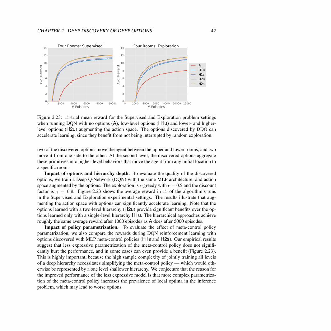
CHAPTER 2. DEEP DISCOVERY OF DEEP OPTIONS 42
Figure 2.23: 15-trial mean reward for the Supervised and Exploration problem settingswhen running DQN with no options (A), low-level options (H1u) and lower- and higher-level options (H2u) augmenting the action space. The options discovered by DDO canaccelerate learning, since they benefit from not being interrupted by random exploration.
two of the discovered options move the agent between the upper and lower rooms, and twomove it from one side to the other. At the second level, the discovered options aggregatethese primitives into higher-level behaviors that move the agent from any initial location toa specific room.
Impact of options and hierarchy depth. To evaluate the quality of the discoveredoptions, we train a Deep Q-Network (DQN) with the same MLP architecture, and actionspace augmented by the options. The exploration is ε-greedy with ε “ 0.2 and the discountfactor is γ “ 0.9. Figure 2.23 shows the average reward in 15 of the algorithm’s runsin the Supervised and Exploration experimental settings. The results illustrate that aug-menting the action space with options can significantly accelerate learning. Note that theoptions learned with a two-level hierarchy (H2u) provide significant benefits over the op-tions learned only with a single-level hierarchy H1u. The hierarchical approaches achieveroughly the same average reward after 1000 episodes as A does after 5000 episodes.
Impact of policy parametrization. To evaluate the effect of meta-control policyparametrization, we also compare the rewards during DQN reinforcement learning withoptions discovered with MLP meta-control policies (H1s and H2s). Our empirical resultssuggest that less expressive parametrization of the meta-control policy does not signifi-cantly hurt the performance, and in some cases can even provide a benefit (Figure 2.23).This is highly important, because the high sample complexity of jointly training all levelsof a deep hierarchy necessitates simplifying the meta-control policy — which would oth-erwise be represented by a one level shallower hierarchy. We conjecture that the reason forthe improved performance of the less expressive model is that more complex parametriza-tion of the meta-control policy increases the prevalence of local optima in the inferenceproblem, which may lead to worse options.
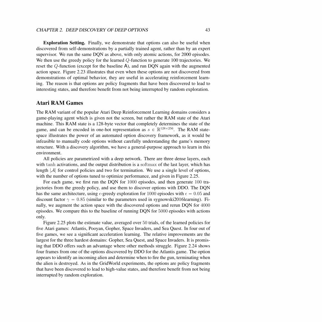
CHAPTER 2. DEEP DISCOVERY OF DEEP OPTIONS 43
Exploration Setting. Finally, we demonstrate that options can also be useful whendiscovered from self-demonstrations by a partially trained agent, rather than by an expertsupervisor. We run the same DQN as above, with only atomic actions, for 2000 episodes.We then use the greedy policy for the learned Q-function to generate 100 trajectories. Wereset the Q-function (except for the baseline A), and run DQN again with the augmentedaction space. Figure 2.23 illustrates that even when these options are not discovered fromdemonstrations of optimal behavior, they are useful in accelerating reinforcement learn-ing. The reason is that options are policy fragments that have been discovered to lead tointeresting states, and therefore benefit from not being interrupted by random exploration.
Atari RAM GamesThe RAM variant of the popular Atari Deep Reinforcement Learning domains considers agame-playing agent which is given not the screen, but rather the RAM state of the Atarimachine. This RAM state is a 128-byte vector that completely determines the state of thegame, and can be encoded in one-hot representation as s P R128ˆ256. The RAM state-space illustrates the power of an automated option discovery framework, as it would beinfeasible to manually code options without carefully understanding the game’s memorystructure. With a discovery algorithm, we have a general-purpose approach to learn in thisenvironment.
All policies are parametrized with a deep network. There are three dense layers, eachwith tanh activations, and the output distribution is a softmax of the last layer, which haslength |A| for control policies and two for termination. We use a single level of options,with the number of options tuned to optimize performance, and given in Figure 2.25.
For each game, we first run the DQN for 1000 episodes, and then generate 100 tra-jectories from the greedy policy, and use them to discover options with DDO. The DQNhas the same architecture, using ε-greedy exploration for 1000 episodes with ε “ 0.05 anddiscount factor γ “ 0.85 (similar to the parameters used in sygnowski2016learning). Fi-nally, we augment the action space with the discovered options and rerun DQN for 4000episodes. We compare this to the baseline of running DQN for 5000 episodes with actionsonly.
Figure 2.25 plots the estimate value, averaged over 50 trials, of the learned policies forfive Atari games: Atlantis, Pooyan, Gopher, Space Invaders, and Sea Quest. In four out offive games, we see a significant acceleration learning. The relative improvements are thelargest for the three hardest domains: Gopher, Sea Quest, and Space Invaders. It is promis-ing that DDO offers such an advantage where other methods struggle. Figure 2.24 showsfour frames from one of the options discovered by DDO for the Atlantis game. The optionappears to identify an incoming alien and determine when to fire the gun, terminating whenthe alien is destroyed. As in the GridWorld experiments, the options are policy fragmentsthat have been discovered to lead to high-value states, and therefore benefit from not beinginterrupted by random exploration.
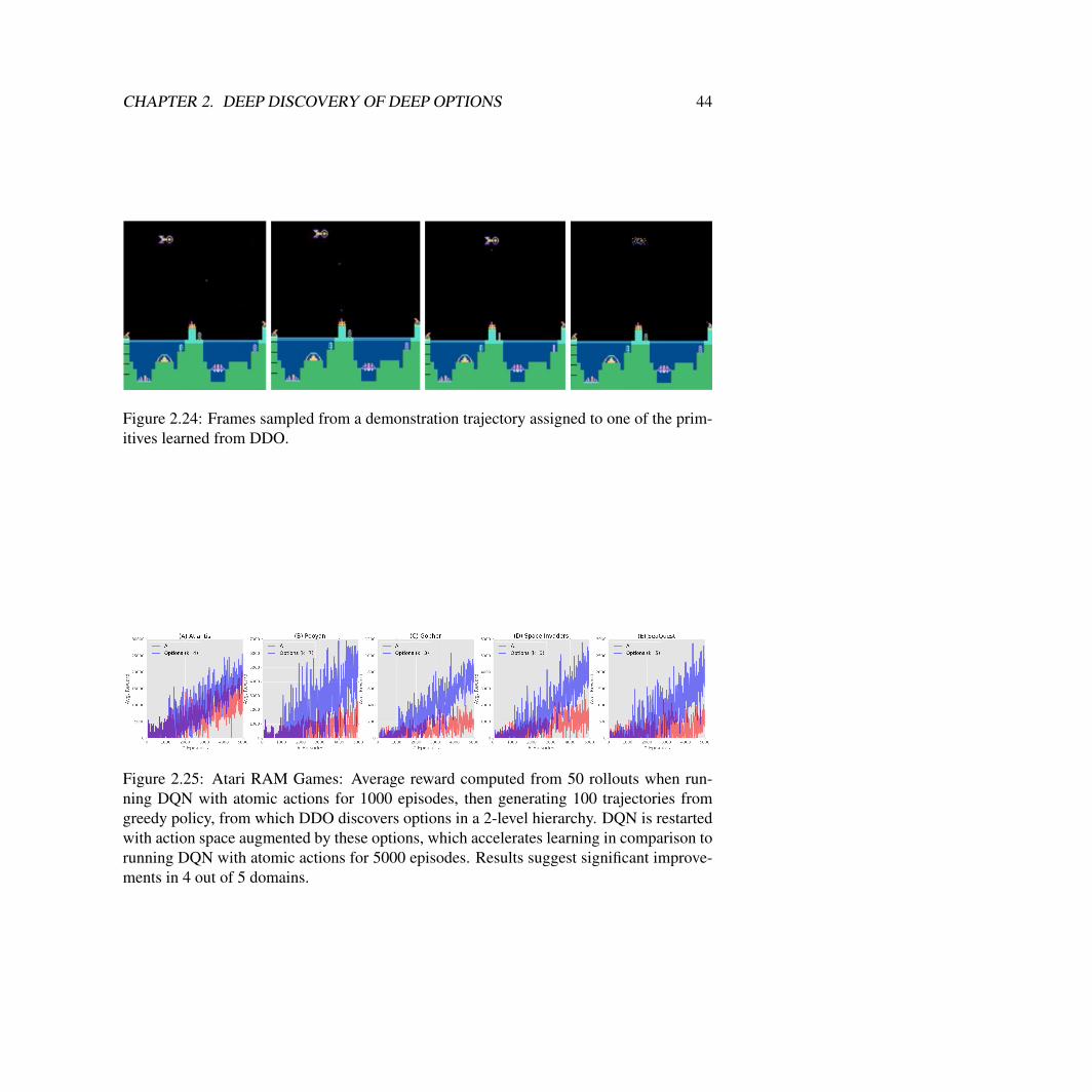
CHAPTER 2. DEEP DISCOVERY OF DEEP OPTIONS 44
Figure 2.24: Frames sampled from a demonstration trajectory assigned to one of the prim-itives learned from DDO.
Figure 2.25: Atari RAM Games: Average reward computed from 50 rollouts when run-ning DQN with atomic actions for 1000 episodes, then generating 100 trajectories fromgreedy policy, from which DDO discovers options in a 2-level hierarchy. DQN is restartedwith action space augmented by these options, which accelerates learning in comparison torunning DQN with atomic actions for 5000 episodes. Results suggest significant improve-ments in 4 out of 5 domains.
Chapter 3
Sequential Windowed InverseReinforcement Learning:Learning Reward DecompositionFrom Data
In the previous chapter, I considered a model where sequences of state-action tuples froman expert demonstrator were available. Next, we consider a setting where only the statesequence is observed. This can happen when the demonstration modality differs from theexecution setting, e.g., learning from third person videos, motion capture of a human doinga task, or kinesthetic demonstrations. Thus, the data cannot be directly used to derive acontroller since the actions are not visible. So, we approach this problem with a simplepremise; change in reward function implies change in behavior. Like DDO, we applyunsupervised learning to a small number of initial expert demonstrations to learn a latentreward structure. This requires two pieces: robustly detecting consistent changes in statetrajectories and constructing reward functions around those change points.
As a motivating example from the problem setting consider the widespread adoptionof robot-assisted minimally invasive surgery (RMIS), which is generating datasets of kine-matic and video recordings of surgical procedures [39]. Explicitly modeling the systemdynamics can require learning a large number of parameters. This makes a direct systemidentification approach somewhat sensitive to any noise in the dataset, especially when thedatasets are small. Furthermore, the states are often high-dimensional with combinationsof kinematic and visual features.
Suppose, one could decompose a surgical task into a consistent sequence of sub-tasks.While each demonstration motion may vary and be noisy, each demonstration also con-tains roughly the same order of true segments. This consistent, repeated structure can beexploited to infer global segmentation criteria. By assuming known sequential segment-to-
45
CHAPTER 3. SWIRL 46
segment ordering, the problem reduces to identifying a common set of segment-to-segmenttransition events–not corresponding entire the trajectory segments across the whole dataset.This allows us to apply coarser, imperfect motion-based segmentation algorithms first thatcreate a large set of candidate transitions. Then, we can filter this set by identifying tran-sition events that occurred at similar times and states. Our experiments suggest that thisapproach has improved robustness and sample-efficiency, while approximating the behav-ior of more complicated dynamical systems-based approaches in many real problems.
I formalize this intuition into a new hierarchical clustering algorithm for unsupervisedsegmentation called Transition State Clustering. The proposed approach is also relevant toproblems in other domains, but I will focus on results from surgical applications. TSC firstapplies a motion-based segmentation model over the noisy trajectories and identifies a set ofcandidate segment transitions in each. TSC then clusters the transition states (states at timestransitions occur) in terms of kinematic, sensory, and temporal similarity. The clusteringprocess is hierarchical where the transition states are first assigned to Gaussian Mixtureclusters according to kinematic state, then these clusters are sub-divided using the sensoryfeatures, and finally by time. We present experiments where these sensory features areconstructed from video. The learned clustering model can be applied to segment previouslyunseen trajectories by the same global criteria. To avoid setting the number of clusters ateach level of the hierarchy in advance, the number of regions are determined by a DirichletProcess prior. A series of merging and pruning steps remove sparse clusters and repetitiveloops.
3.1 Transition State Clustering
This section describes the problem setting, assumptions, and notation. Let D “ tdiu be aset of demonstrations of a robotic task. Each demonstration of a task d is a discrete-timesequence of T state vectors in a feature-space X . The feature space is a concatenationof kinematic features X (e.g., robot position) and sensory features V (e.g., visual featuresfrom the environment).
Definition 1 (Segmentation) A segmentation of a task is defined as a function S that as-signs each state in every demonstration trajectory to an integer 1, 2, ..., k:
S : d ÞÑ panq1,...,|d|, an P 1, ..., k.
and S is a non-decreasing function in time (no repetitions).
Suppose we are given a function that just identifies candidate segment endpoints basedon the kinematic features. Such a function is weaker than a segmentation function since itdoes not globally label the detected segments. This leads to the following definition:
Definition 2 (Transition Indicator Function) A transition indicator function T is a func-tion that maps each kinematic state in a demonstration d to t0, 1u:
T : d ÞÑ panq1,...,|d|, an P 0, 1.

CHAPTER 3. SWIRL 47
The above definition naturally leads to a notion of transition states, the states and timesat which transitions occur.
Definition 3 (Transition States) For a demonstration di, let oi,t denote the kinematic state,visual state, and time px, v, tq at time t. Transition States are the set of state-time tupleswhere the indicator is 1:
Γ “Nď
i
toi,t P di : Tpdiqt “ 1u.
The goal of TSC is to take the transition states Γ and recover a segmentation function S.This segmentation function is stronger than the provided T since it not only indicates that atransition has occurred but labels the segment transition consistently across demonstrations.
AssumptionsWe assume that all possible true segments are represented in each demonstration by at leastone transition (some might be false positives). Given the segmentation function Spdiq, onecan define a set of true transition states:
Γ˚ “ toi,t P di : Spdiqt´1 ‰ Spdiqt, t ą 0u.
These satisfy the following property:
Γ˚ Ď Γ.
In other words, we assume that a subset of transition states discovered by the indicatorfunction correspond with the true segment transitions. There can be false positives butno false negatives (a demonstration where a segment transition is missed by the transitionindicator function). Since the segmentation function is sequential and in a fixed order, thisleads to a model where we are trying to find the k ´ 1 true segment-segment transitionpoints in Γ.
Problem Statement and Method OverviewThese definitions allow us to formalize the transition state clustering problem.
Problem 2 (Transition State Clustering) Given a set of regular demonstrations D andtransition identification function T, find a segmentation S.
Candidate Transitions: To implement T, TSC fits a Gaussian mixture model to slidingwindows over each of the demonstration trajectories and identifies consecutive times withdifferent most-likely mixture components.
CHAPTER 3. SWIRL 48
Algorithm 1 Transition Identification1: Input: D demonstrations, ` a window size, and α a Dirichlet Process prior.2: For each demonstration, generate a set of sliding windows of wp`q
t “ rxt´`, ...,xtsᵀ.
Let W be the set of all sliding windows across all demonstrations.3: Fit a mixture model to W assigning each state to its most likely component.4: Identify times t in each demonstration when wt has a different most likely mixture
component than wt`1, start and finish times (t “ 0, t “ Ti) are automatically transi-tions.
5: Return: A set of transition states Γ, the px, v, tq tuples at which transitions occur.
Transition State Clusters: The states at which those transitions occur are called transitionstates. TSC uses a GMM to cluster the transition states in terms of spatial and temporalsimilarity to find S.Optimizations: To avoid setting the number of clusters at each level of the hierarchy inadvance, the number of regions are determined by a Dirichlet Process prior. A series ofmerging and pruning steps remove sparse clusters and repetitive loops.
Gaussian Mixture Transition IdentificationWhile we can use any transition identification function to get Γ (as long as it satisfies theassumptions), we present one implementation based of Gaussian Mixtures that we used ina number of our experiments. We found that this GMM approach was scalable (in termsof data and dimensionality) and had fewer hyper-parameters to tune than more complexmodels. Combined with the subsequent hierarchical clustering, this approach proved to berobust in all of our experiments.
Each demonstration trajectory di is a trajectory of Ti state-vectors rx1, ..., xTis. For agiven time t, we can define a window of length ` as:
wp`qt “ rst´`, ..., sts
ᵀ
We can further normalize this window relative to its first state:
np`qt “ rst´` ´ st´`, ..., st ´ st´`s
ᵀ
This represents the “delta” in movement over the time span of a window. Then, for eachdemonstration trajectory we can also generate a trajectory of T ´ ` windowed states:
dp`q “ rnp`q` , ...,n
p`qT s
Over the entire set of windowed demonstrations, we collect a dataset of all of the np`qt
vectors. We fit a GMM model to these vectors. The GMM model defines m multivariateGaussian distributions and a probability that each observation n
p`qt is sampled from each

CHAPTER 3. SWIRL 49
Algorithm 2 Transition State ClusteringInput: Γ Transition States, ρ pruning parameterFit a mixture model to the set of transition states Γ in the kinematic states.Fit a mixture model to the sensory features for transitions within every kinematic clusteri.Fit a mixture model to the times from every kinematic and sensory cluster pair pi, jq.Remove clusters that contain fewer than transition states from fewer than ρ ¨ N distinctdemonstrations.Output: A set of transitions, which are regions of the state-space and temporal intervalsdefined by Gaussian confidence intervals.
of the m distributions. We annotate each observation with the most likely mixture com-ponent. Times such that np`qt and n
p`qt`1 have different most likely components are marked
as transitions. This model captures some dynamical behaviors while not requiring explicitmodeling of the state-to-state transition function.
Sometimes the MDP’s states are more abstract and do not map to space where the nor-malized windows make sense. We can still apply the same method when we only have apositive definite kernel function over all pairs of states κpsi, sjq. We can construct this ker-nel function for all of the states observed in the demonstrations and apply Kernelized PCAto the features before learning the transitions–a technique used in Computer Vision [84].The top p1 eigenvalues define a new embedded feature vector for each ω in Rp1 . We cannow apply the algorithm above in this embedded feature space.
TSC Inference AlgorithmWe present the clustering algorithm which is summarized in Algorithm 2. In a first pass,the transition states are clustered with respect to the kinematic states, then sub-clusteredwith respect to the sensory states, and then, we temporally sub-cluster. The sub-clusterscan be used to formulate the segmentation criteria.
Kinematic Step: We want our model to capture that transitions that occur in similarpositions in the state-space across all demonstrations are actual transitions, and we wouldlike to aggregate these transitions into logical events. Hypothetically, if we had infinitedemonstrations Γ would define a density of transition events throughout the state-space.The modes of the density, which intuitively represent a propensity of a state x to trigger asegment change, are of key interest to us.
We can think of the set of identified transition states Γ as a sample of this density. Wefit a DP-GMM to kinematic features of the transition states. Each transition state will havean assignment probability to one of the mixture components. We convert this to a hardassignment by assigning the transition state to the most likely component.
Sensory Step: Then, we apply the second level of DP-GMM fitting over the sensory fea-tures (if available). Within each kinematic cluster, we fit a DP-GMM to find sub-clusters in
CHAPTER 3. SWIRL 50
the sensory features. Note that the transitions were only identified with kinematic features.This step grounds the detected transitions in sensory clusters.
Temporal Step: Finally, we apply the last level of DP-GMM fitting over the time axis.Without temporal localization, the transitions may be ambiguous. For example, in a figure8 motion, the robot may pass over a point twice in the same task. Conditioned on theparticular state-space cluster assignment, we can fit a DP-GMM each to each subset oftimes. The final result contains sub-clusters that are indexed both in the state-space and intime.
Enforcing Consistency: The learned clusters will vary in size as some may consist oftransitions that appear only in a few demonstrations. The goal of TSC is to identify thoseclusters that correspond to state and time transition conditions common to all demonstra-tions of a task. We frame this as a pruning problem, where we want to enforce that alllearned clusters contain transitions from a fraction of ρ distinct demonstrations. Clusterswhose constituent transition states come from fewer than a fraction ρ demonstrations arepruned. ρ should be set based on the expected rarity of outliers. For example, if ρ is 100%then the only mixture components that are found are those with at least one transition statefrom every demonstration (i.e., the regularity assumption). If ρ is less than 100%, then itmeans that every mixture component must cover some subset of the demonstrations. In ourexperiments, we set the parameter ρ to 80% and show the results with and without this step.
Segmentation Criteria: Finally, if there are k remaining clusters tC1, ..., Cku, we canuse these clusters to form a criteria for segmentation. Each cluster is formed using a GMMtriplet in the kinematic state, visual state, and time. The quantiles of the three GMMs willdefine an ordered sequence of regions rρ1, ..., ρks over the state-space and each of theseregions has an associated time interval defined by the Gaussian confidence interval forsome confidence level zα.
TSC Simulated Experimental EvaluationWe evaluate TSC’s robustness in the following way:
1. Precision. Results suggest TSC significantly reduces the number of false positivesegments in simulated examples with noise.
2. Recall. Among algorithms that use piecewise linear segment models, results suggestTSC recovers segments of a generated piecewise linear trajectory more consistentlyin the presence of process and observation noise.
3. Applicability to Real-World Data. Result suggest that TSC recovers qualitativelyrelevant segments in real surgical trajectory data.

CHAPTER 3. SWIRL 51
Precision in Synthetic Examples
Our first experiment evaluates the following hypothesis: TSC significantly reduces thenumber of false positive segments in a simple simulated example with noise. These exper-iments evaluate TSC against algorithms with a single level of clustering.
Comparison of 7 alternative segmentation criteria:
1. Zero-Velocity Crossing (VEL): This algorithm detects a change in the sign of thevelocity.
2. Smoothed Zero-Velocity Crossing (VELS): This algorithm applies a low-pass filter(exponentially weighted moving average) to the trajectory, and then detects a changein the sign of the velocity.
3. Acceleration (ACC): This algorithm detects any change in the velocity by lookingfor non-zero acceleration.
4. Gaussian Mixture Model (GMM): This algorithm applies a GMM model to the ob-served states and detects changes in most likely assignment. The number of clusterswere set to 2.
5. Windowed Gaussian Mixture Model (GMMW): This algorithm is the first phase ofTSC. It applies a GMM to windows of size 2, and detects changes in most likelyassignment. The number of clusters was set to 2, unlike in TSC where we use the DPto set the number of clusters.
6. Auto-Regressive Mixture (AR): This model fits a piecewise linear transition law tothe observed data.
7. Coresets (CORE): We evaluate against a standard coreset model [120, 130], and theparticular variant is implemented with weighted k-means. We applied this to thesame augmented state-vector as in the previously mentioned GMM.
8. TSC: Our proposed approach with a pruning threshold of 0.8 and no loop com-paction.
Bouncing Ball: We first revisit the example in the introduction of the bouncing ball,which can be modeled as the following 1D double-integrator system:
:x “ r´9.8s22
This system is observed with additive Gaussian white noise with std. 10 (Moderate Noise):
y “ x`Np0, 10q
and std. 20 (High Noise):y “ x`Np0, 20q
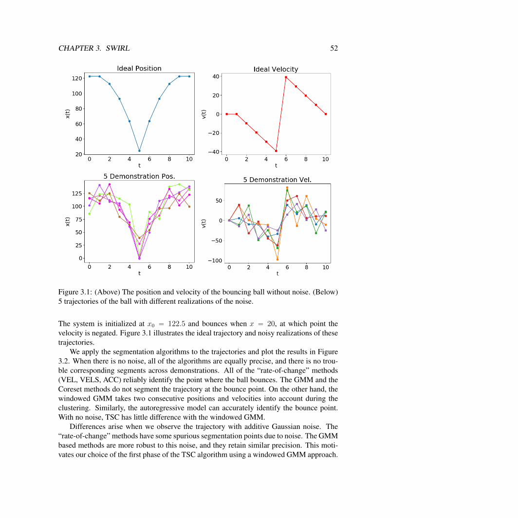
CHAPTER 3. SWIRL 52
Figure 3.1: (Above) The position and velocity of the bouncing ball without noise. (Below)5 trajectories of the ball with different realizations of the noise.
The system is initialized at x0 “ 122.5 and bounces when x “ 20, at which point thevelocity is negated. Figure 3.1 illustrates the ideal trajectory and noisy realizations of thesetrajectories.
We apply the segmentation algorithms to the trajectories and plot the results in Figure3.2. When there is no noise, all of the algorithms are equally precise, and there is no trou-ble corresponding segments across demonstrations. All of the “rate-of-change” methods(VEL, VELS, ACC) reliably identify the point where the ball bounces. The GMM and theCoreset methods do not segment the trajectory at the bounce point. On the other hand, thewindowed GMM takes two consecutive positions and velocities into account during theclustering. Similarly, the autoregressive model can accurately identify the bounce point.With no noise, TSC has little difference with the windowed GMM.
Differences arise when we observe the trajectory with additive Gaussian noise. The“rate-of-change” methods have some spurious segmentation points due to noise. The GMMbased methods are more robust to this noise, and they retain similar precision. This moti-vates our choice of the first phase of the TSC algorithm using a windowed GMM approach.
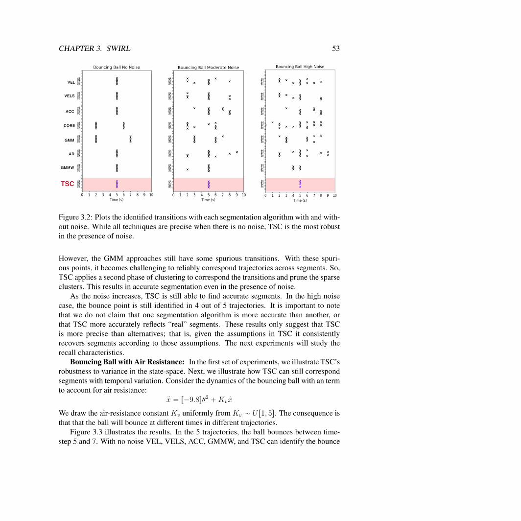
CHAPTER 3. SWIRL 53
Figure 3.2: Plots the identified transitions with each segmentation algorithm with and with-out noise. While all techniques are precise when there is no noise, TSC is the most robustin the presence of noise.
However, the GMM approaches still have some spurious transitions. With these spuri-ous points, it becomes challenging to reliably correspond trajectories across segments. So,TSC applies a second phase of clustering to correspond the transitions and prune the sparseclusters. This results in accurate segmentation even in the presence of noise.
As the noise increases, TSC is still able to find accurate segments. In the high noisecase, the bounce point is still identified in 4 out of 5 trajectories. It is important to notethat we do not claim that one segmentation algorithm is more accurate than another, orthat TSC more accurately reflects “real” segments. These results only suggest that TSCis more precise than alternatives; that is, given the assumptions in TSC it consistentlyrecovers segments according to those assumptions. The next experiments will study therecall characteristics.
Bouncing Ball with Air Resistance: In the first set of experiments, we illustrate TSC’srobustness to variance in the state-space. Next, we illustrate how TSC can still correspondsegments with temporal variation. Consider the dynamics of the bouncing ball with an termto account for air resistance:
:x “ r´9.8s22`Kv 9x
We draw the air-resistance constant Kv uniformly from Kv „ U r1, 5s. The consequence isthat that the ball will bounce at different times in different trajectories.
Figure 3.3 illustrates the results. In the 5 trajectories, the ball bounces between time-step 5 and 7. With no noise VEL, VELS, ACC, GMMW, and TSC can identify the bounce
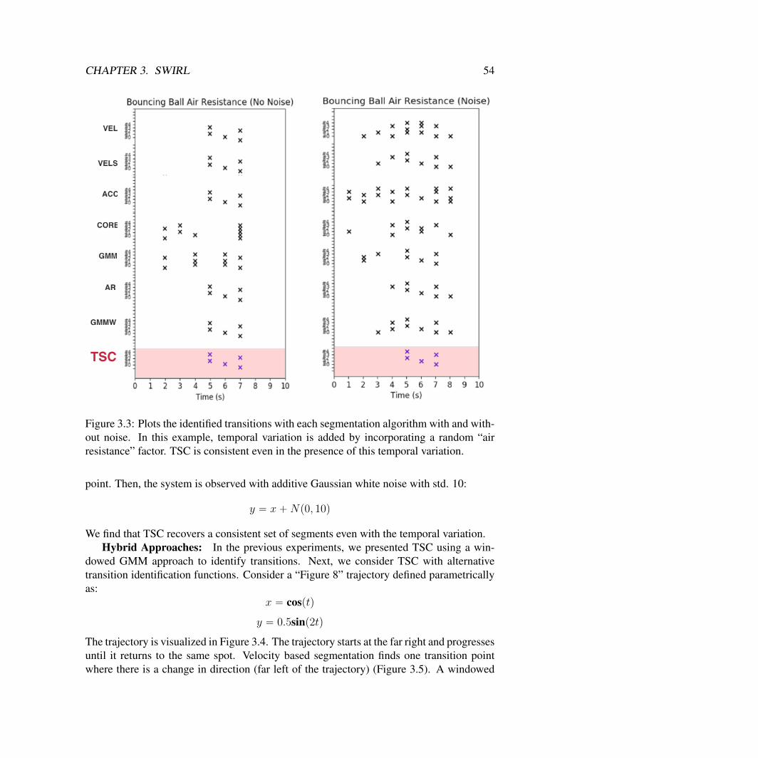
CHAPTER 3. SWIRL 54
Figure 3.3: Plots the identified transitions with each segmentation algorithm with and with-out noise. In this example, temporal variation is added by incorporating a random “airresistance” factor. TSC is consistent even in the presence of this temporal variation.
point. Then, the system is observed with additive Gaussian white noise with std. 10:
y “ x`Np0, 10q
We find that TSC recovers a consistent set of segments even with the temporal variation.Hybrid Approaches: In the previous experiments, we presented TSC using a win-
dowed GMM approach to identify transitions. Next, we consider TSC with alternativetransition identification functions. Consider a “Figure 8” trajectory defined parametricallyas:
x “ cosptq
y “ 0.5sinp2tq
The trajectory is visualized in Figure 3.4. The trajectory starts at the far right and progressesuntil it returns to the same spot. Velocity based segmentation finds one transition pointwhere there is a change in direction (far left of the trajectory) (Figure 3.5). A windowed

CHAPTER 3. SWIRL 55
Figure 3.4: A “figure 8” trajectory in the plane, and 5 noisy demonstrations. The trajectorystarts at the far right and progresses until it returns to the same spot.
Figure 3.5: Plots the identified transitions with each segmentation algorithm with and with-out noise. Velocity based segmentation finds one transition point where there is a changein direction. A windowed GMM where the number of clusters is set by a DP finds threetransition points. TSC can improve the precision of both techniques.
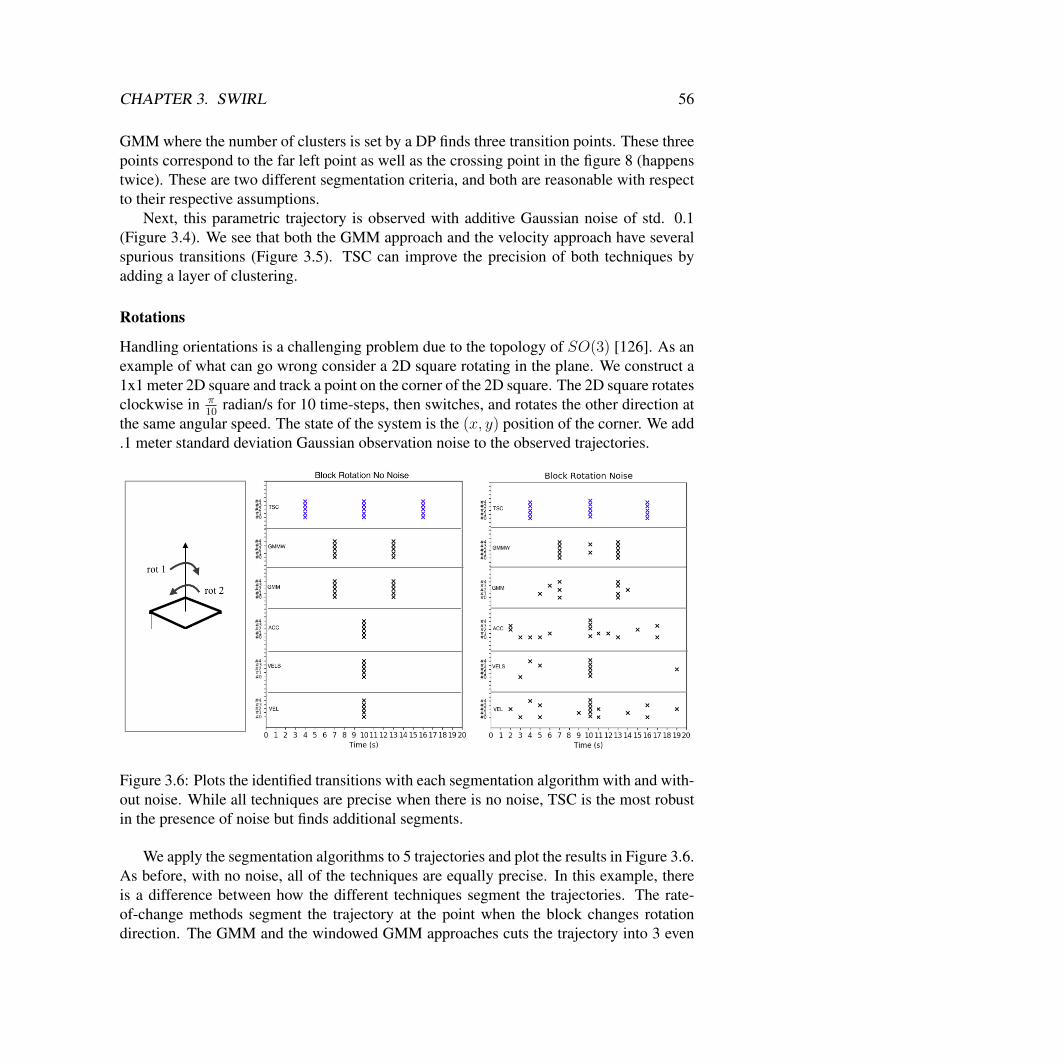
CHAPTER 3. SWIRL 56
GMM where the number of clusters is set by a DP finds three transition points. These threepoints correspond to the far left point as well as the crossing point in the figure 8 (happenstwice). These are two different segmentation criteria, and both are reasonable with respectto their respective assumptions.
Next, this parametric trajectory is observed with additive Gaussian noise of std. 0.1(Figure 3.4). We see that both the GMM approach and the velocity approach have severalspurious transitions (Figure 3.5). TSC can improve the precision of both techniques byadding a layer of clustering.
Rotations
Handling orientations is a challenging problem due to the topology of SOp3q [126]. As anexample of what can go wrong consider a 2D square rotating in the plane. We construct a1x1 meter 2D square and track a point on the corner of the 2D square. The 2D square rotatesclockwise in π
10radian/s for 10 time-steps, then switches, and rotates the other direction at
the same angular speed. The state of the system is the px, yq position of the corner. We add.1 meter standard deviation Gaussian observation noise to the observed trajectories.
Figure 3.6: Plots the identified transitions with each segmentation algorithm with and with-out noise. While all techniques are precise when there is no noise, TSC is the most robustin the presence of noise but finds additional segments.
We apply the segmentation algorithms to 5 trajectories and plot the results in Figure 3.6.As before, with no noise, all of the techniques are equally precise. In this example, thereis a difference between how the different techniques segment the trajectories. The rate-of-change methods segment the trajectory at the point when the block changes rotationdirection. The GMM and the windowed GMM approaches cuts the trajectory into 3 even
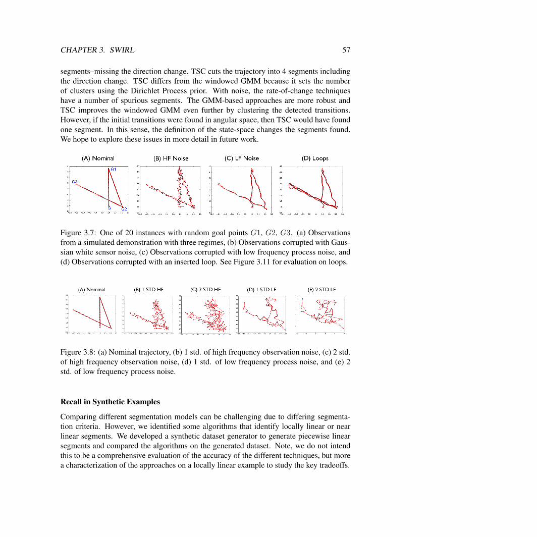
CHAPTER 3. SWIRL 57
segments–missing the direction change. TSC cuts the trajectory into 4 segments includingthe direction change. TSC differs from the windowed GMM because it sets the numberof clusters using the Dirichlet Process prior. With noise, the rate-of-change techniqueshave a number of spurious segments. The GMM-based approaches are more robust andTSC improves the windowed GMM even further by clustering the detected transitions.However, if the initial transitions were found in angular space, then TSC would have foundone segment. In this sense, the definition of the state-space changes the segments found.We hope to explore these issues in more detail in future work.
Figure 3.7: One of 20 instances with random goal points G1, G2, G3. (a) Observationsfrom a simulated demonstration with three regimes, (b) Observations corrupted with Gaus-sian white sensor noise, (c) Observations corrupted with low frequency process noise, and(d) Observations corrupted with an inserted loop. See Figure 3.11 for evaluation on loops.
Figure 3.8: (a) Nominal trajectory, (b) 1 std. of high frequency observation noise, (c) 2 std.of high frequency observation noise, (d) 1 std. of low frequency process noise, and (e) 2std. of low frequency process noise.
Recall in Synthetic Examples
Comparing different segmentation models can be challenging due to differing segmenta-tion criteria. However, we identified some algorithms that identify locally linear or nearlinear segments. We developed a synthetic dataset generator to generate piecewise linearsegments and compared the algorithms on the generated dataset. Note, we do not intendthis to be a comprehensive evaluation of the accuracy of the different techniques, but morea characterization of the approaches on a locally linear example to study the key tradeoffs.
CHAPTER 3. SWIRL 58
We model the trajectory of a point robot with two-dimensional position state px, yq be-tween k goal points tg1, ..., gku. We apply position control to guide the robot to the targetsand without disturbance, this motion is linear (Figure 3.7a). We add various types of dis-turbances (and in varying amounts) including Gaussian observation noise, low-frequencyprocess noise, and repetitive loops (Figure 3.7b-d). We report noise values in terms ofstandard deviations. Figure 3.8 illustrates the relative magnitudes. A demonstration di is asample from the following system.
Task: Every segmentation algorithm will be evaluated in its ability to identify the k ´ 1segments (i.e., the paths between the goal points). Furthermore, we evaluate algorithms onrandom instances of this task. In the beginning, we select 3 random goal points. From afixed initial position, we control the simulated point robot to the goal points with positioncontrol. Without any disturbance, this follows a linear motion. For a given noise setting,we sample demonstrations from this system and apply/evaluate each algorithm. We presentresults aggregated over 20 such random instances. This is important since many of thesegmentation algorithms proposed in literature have some crucial hyper-parameters, andwe present results with a single choice of parameters averaged over multiple tasks. Thisway, the hyper-parameter tuning cannot overfit to any given instance of the problem and hasto be valid for the entire class of tasks. We believe that this is important since tuning thesehyper-parameters in practice (i.e., not in simulation) is challenging since there is no groundtruth. The experimental code is available at: http://berkeleyautomation.github.io/tsc/.
5 Algorithms: We compare TSC against alternatives where the authors explicitly find (orapproximately find) locally linear segments. It is important to reiterate that different seg-mentation techniques optimize different objectives, and this benchmark is meant to char-acterize the performance on a common task. All of the techniques are based on GaussianDistributions or Linear auto-regressive models.
1. (GMM) (Same as previous experiment). In this experiment, we set the parameter tothe optimal choice of 3 without automatic tuning.
2. (GMM+HMM) A natural extension to this model is to enforce a transition structureon the regimes with a latent Markov Chain [4, 21, 71, 127]. We use the same statevector as above, without time augmentation as this is handled by the HMM. We fitthe model using the forward-backward algorithm.
3. Coresets (Same as previous experiment).
4. HSMM We evaluated a Gaussian Hidden Semi-Markov Model. We directly appliedthis model to the demonstrations with no augmentation or normalization of features.This was implemented with the package pyhsmm. We directly applied this modelto the demonstrations with no augmentation as in the GMM approaches. We ranour MCMC sampler for 10000 iterations, discarding the first 2500 as burn-in andthinning the chain by 15.
CHAPTER 3. SWIRL 59
5. AR-HMM We evaluated a Bayesian Autoregressive HMM model as used in [89].This was implemented with the packages pybasicbayes and pyhsmm-ar. The au-toregressive order was 10 and we ran our MCMC sampler for 10000 iterations, dis-carding the first 2500 as burn-in and thinning the chain by 15.
Evaluation Metric: There is considerable debate on metrics to evaluate the accuracyof unsupervised segmentation and activity recognition techniques, e.g. frame accuracywu2015watch, hamming distance fox2009sharing. Typically, these metrics have two steps:(1) segments to ground truth correspondence, and (2) then measuring the similarity be-tween corresponded segments. We have made this feature extensible and evaluated somedifferent accuracy metrics (Jaccard Similarity, Frame Accuracy, Segment Accuracy, Inter-section over Union). We found that the following procedure led to the most insightfulresults–differentiating the different techniques.
In the first phase, we match segments in our predicted sequence to those in the groundtruth. We do this with a procedure identical to the one proposed in [132]. We define abi-partite graph of predicted segments to ground truth segments, and add weighted edgeswhere weights represent the overlap between a predicted segment and a ground-truth seg-ment (i.e., the recall over time-steps). Each predicted segment is matched to its highestweighted ground truth segment. Each predicted segment is assigned to exactly one ground-truth segment, while a ground-truth segment may have none, one, or more correspondingpredictions.
After establishing the correspondence between predictions and ground truth, we con-sider a true positive (a ground-truth segment is correctly identified) if the overlap (intersection-over-union) between the ground-truth segment and its corresponding predicted segments ismore than a default threshold 60%. Then, we compute Segment Accuracy as the ratioof the ground-truth segments that are correctly detected. In [132], the authors use a 40%threshold but apply the metric to real data. Since this is a synthetic example, we increasethis threshold to 60%, which we empirically found accounted for boundary effects espe-cially in the Bayesian approaches (i.e., repeated transitions around segment endpoints).
Accuracy vs. Noise
In our first experiment, we measured the segment accuracy for each of the algorithms for50 demonstrations. We also varied the amount of process and observation noise in thesystem. As Figure 3.8 illustrates, this is a very significant amount of noise in the data,and successful techniques must exploit the structure in multiple demonstrations. Figure3.9a illustrates the performance of each of the techniques as a function of high-frequencyobservation noise. Results suggest that TSC is more robust to noise than the alternatives(nearly 20% more accurate for 2.5 std of noise). The Bayesian ARHMM approach is nearlyidentical to TSC when the noise is low but quickly loses accuracy as more noise is added.We attribute this robustness to the TSC’s pruning step which ensures that only transitionstate clusters with sufficient coverage across all demonstrations are kept. These results
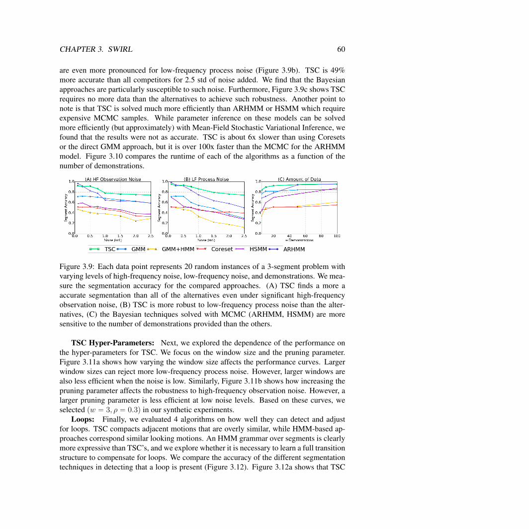
CHAPTER 3. SWIRL 60
are even more pronounced for low-frequency process noise (Figure 3.9b). TSC is 49%more accurate than all competitors for 2.5 std of noise added. We find that the Bayesianapproaches are particularly susceptible to such noise. Furthermore, Figure 3.9c shows TSCrequires no more data than the alternatives to achieve such robustness. Another point tonote is that TSC is solved much more efficiently than ARHMM or HSMM which requireexpensive MCMC samples. While parameter inference on these models can be solvedmore efficiently (but approximately) with Mean-Field Stochastic Variational Inference, wefound that the results were not as accurate. TSC is about 6x slower than using Coresetsor the direct GMM approach, but it is over 100x faster than the MCMC for the ARHMMmodel. Figure 3.10 compares the runtime of each of the algorithms as a function of thenumber of demonstrations.
Figure 3.9: Each data point represents 20 random instances of a 3-segment problem withvarying levels of high-frequency noise, low-frequency noise, and demonstrations. We mea-sure the segmentation accuracy for the compared approaches. (A) TSC finds a more aaccurate segmentation than all of the alternatives even under significant high-frequencyobservation noise, (B) TSC is more robust to low-frequency process noise than the alter-natives, (C) the Bayesian techniques solved with MCMC (ARHMM, HSMM) are moresensitive to the number of demonstrations provided than the others.
TSC Hyper-Parameters: Next, we explored the dependence of the performance onthe hyper-parameters for TSC. We focus on the window size and the pruning parameter.Figure 3.11a shows how varying the window size affects the performance curves. Largerwindow sizes can reject more low-frequency process noise. However, larger windows arealso less efficient when the noise is low. Similarly, Figure 3.11b shows how increasing thepruning parameter affects the robustness to high-frequency observation noise. However, alarger pruning parameter is less efficient at low noise levels. Based on these curves, weselected pw “ 3, ρ “ 0.3q in our synthetic experiments.
Loops: Finally, we evaluated 4 algorithms on how well they can detect and adjustfor loops. TSC compacts adjacent motions that are overly similar, while HMM-based ap-proaches correspond similar looking motions. An HMM grammar over segments is clearlymore expressive than TSC’s, and we explore whether it is necessary to learn a full transitionstructure to compensate for loops. We compare the accuracy of the different segmentationtechniques in detecting that a loop is present (Figure 3.12). Figure 3.12a shows that TSC
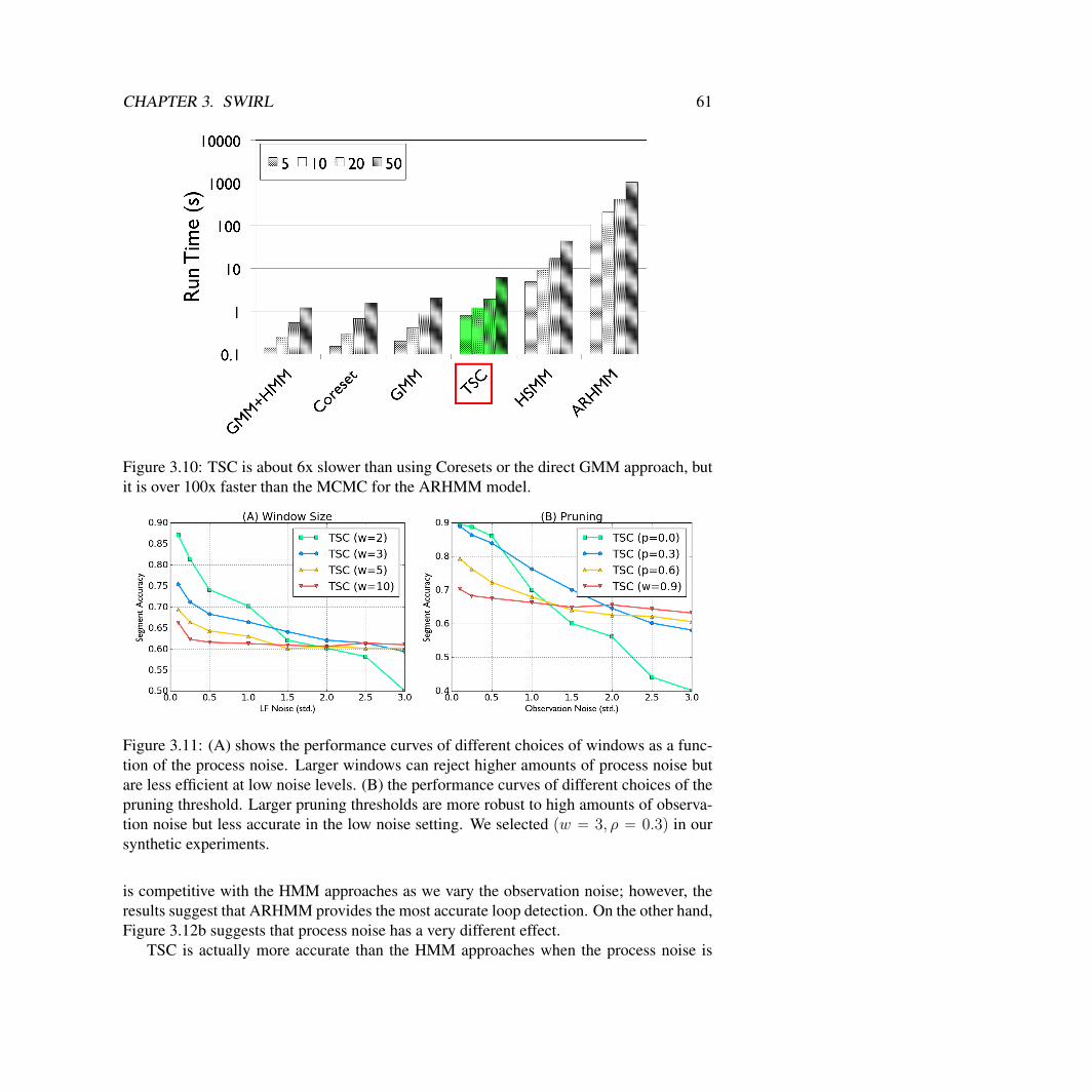
CHAPTER 3. SWIRL 61
Figure 3.10: TSC is about 6x slower than using Coresets or the direct GMM approach, butit is over 100x faster than the MCMC for the ARHMM model.
Figure 3.11: (A) shows the performance curves of different choices of windows as a func-tion of the process noise. Larger windows can reject higher amounts of process noise butare less efficient at low noise levels. (B) the performance curves of different choices of thepruning threshold. Larger pruning thresholds are more robust to high amounts of observa-tion noise but less accurate in the low noise setting. We selected pw “ 3, ρ “ 0.3q in oursynthetic experiments.
is competitive with the HMM approaches as we vary the observation noise; however, theresults suggest that ARHMM provides the most accurate loop detection. On the other hand,Figure 3.12b suggests that process noise has a very different effect.
TSC is actually more accurate than the HMM approaches when the process noise is
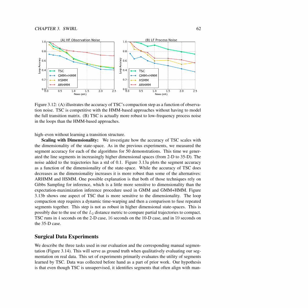
CHAPTER 3. SWIRL 62
Figure 3.12: (A) illustrates the accuracy of TSC’s compaction step as a function of observa-tion noise. TSC is competitive with the HMM-based approaches without having to modelthe full transition matrix. (B) TSC is actually more robust to low-frequency process noisein the loops than the HMM-based approaches.
high–even without learning a transition structure.Scaling with Dimensionality: We investigate how the accuracy of TSC scales with
the dimensionality of the state-space. As in the previous experiments, we measured thesegment accuracy for each of the algorithms for 50 demonstrations. This time we gener-ated the line segments in increasingly higher dimensional spaces (from 2-D to 35-D). Thenoise added to the trajectories has a std of 0.1. Figure 3.13a plots the segment accuracyas a function of the dimensionality of the state-space. While the accuracy of TSC doesdecreases as the dimensionality increases it is more robust than some of the alternatives:ARHMM and HSMM. One possible explanation is that both of those techniques rely onGibbs Sampling for inference, which is a little more sensitive to dimensionality than theexpectation-maximization inference procedure used in GMM and GMM+HMM. Figure3.13b shows one aspect of TSC that is more sensitive to the dimensionality. The loopcompaction step requires a dynamic time-warping and then a comparison to fuse repeatedsegments together. This step is not as robust in higher dimensional state-spaces. This ispossibly due to the use of the L2 distance metric to compare partial trajectories to compact.TSC runs in 4 seconds on the 2-D case, 16 seconds on the 10-D case, and in 59 seconds onthe 35-D case.
Surgical Data ExperimentsWe describe the three tasks used in our evaluation and the corresponding manual segmen-tation (Figure 3.14). This will serve as ground truth when qualitatively evaluating our seg-mentation on real data. This set of experiments primarily evaluates the utility of segmentslearned by TSC. Data was collected before hand as a part of prior work. Our hypothesisis that even though TSC is unsupervised, it identifies segments that often align with man-
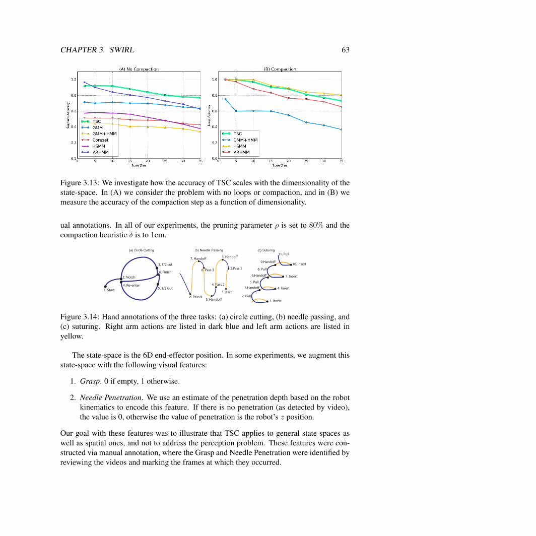
CHAPTER 3. SWIRL 63
Figure 3.13: We investigate how the accuracy of TSC scales with the dimensionality of thestate-space. In (A) we consider the problem with no loops or compaction, and in (B) wemeasure the accuracy of the compaction step as a function of dimensionality.
ual annotations. In all of our experiments, the pruning parameter ρ is set to 80% and thecompaction heuristic δ is to 1cm.
(a) Circle Cutting
1. Start
2. Notch
3. 1/2 cut
4. Re-enter
6. Finish
5. 1/2 Cut
(b) Needle Passing
1.Start
2.Pass 1
3. Hando!
4. Pass 2
5. Hando!
6. Pass 3
7. Hando!
8. Pass 4
1. Insert
2. Pull
3.Hando! 4. Insert
5. Pull
6.Hando! 7. Insert
10. Insert
8. Pull
9.Hando!
11. Pull
(c) Suturing
Figure 3.14: Hand annotations of the three tasks: (a) circle cutting, (b) needle passing, and(c) suturing. Right arm actions are listed in dark blue and left arm actions are listed inyellow.
The state-space is the 6D end-effector position. In some experiments, we augment thisstate-space with the following visual features:
1. Grasp. 0 if empty, 1 otherwise.
2. Needle Penetration. We use an estimate of the penetration depth based on the robotkinematics to encode this feature. If there is no penetration (as detected by video),the value is 0, otherwise the value of penetration is the robot’s z position.
Our goal with these features was to illustrate that TSC applies to general state-spaces aswell as spatial ones, and not to address the perception problem. These features were con-structed via manual annotation, where the Grasp and Needle Penetration were identified byreviewing the videos and marking the frames at which they occurred.
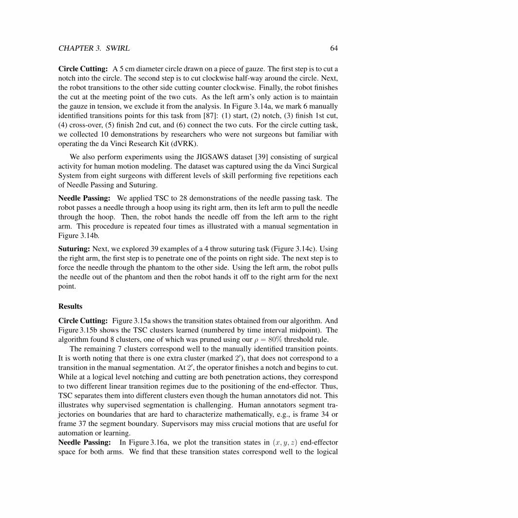
CHAPTER 3. SWIRL 64
Circle Cutting: A 5 cm diameter circle drawn on a piece of gauze. The first step is to cut anotch into the circle. The second step is to cut clockwise half-way around the circle. Next,the robot transitions to the other side cutting counter clockwise. Finally, the robot finishesthe cut at the meeting point of the two cuts. As the left arm’s only action is to maintainthe gauze in tension, we exclude it from the analysis. In Figure 3.14a, we mark 6 manuallyidentified transitions points for this task from [87]: (1) start, (2) notch, (3) finish 1st cut,(4) cross-over, (5) finish 2nd cut, and (6) connect the two cuts. For the circle cutting task,we collected 10 demonstrations by researchers who were not surgeons but familiar withoperating the da Vinci Research Kit (dVRK).
We also perform experiments using the JIGSAWS dataset [39] consisting of surgicalactivity for human motion modeling. The dataset was captured using the da Vinci SurgicalSystem from eight surgeons with different levels of skill performing five repetitions eachof Needle Passing and Suturing.
Needle Passing: We applied TSC to 28 demonstrations of the needle passing task. Therobot passes a needle through a hoop using its right arm, then its left arm to pull the needlethrough the hoop. Then, the robot hands the needle off from the left arm to the rightarm. This procedure is repeated four times as illustrated with a manual segmentation inFigure 3.14b.
Suturing: Next, we explored 39 examples of a 4 throw suturing task (Figure 3.14c). Usingthe right arm, the first step is to penetrate one of the points on right side. The next step is toforce the needle through the phantom to the other side. Using the left arm, the robot pullsthe needle out of the phantom and then the robot hands it off to the right arm for the nextpoint.
Results
Circle Cutting: Figure 3.15a shows the transition states obtained from our algorithm. AndFigure 3.15b shows the TSC clusters learned (numbered by time interval midpoint). Thealgorithm found 8 clusters, one of which was pruned using our ρ “ 80% threshold rule.
The remaining 7 clusters correspond well to the manually identified transition points.It is worth noting that there is one extra cluster (marked 21), that does not correspond to atransition in the manual segmentation. At 21, the operator finishes a notch and begins to cut.While at a logical level notching and cutting are both penetration actions, they correspondto two different linear transition regimes due to the positioning of the end-effector. Thus,TSC separates them into different clusters even though the human annotators did not. Thisillustrates why supervised segmentation is challenging. Human annotators segment tra-jectories on boundaries that are hard to characterize mathematically, e.g., is frame 34 orframe 37 the segment boundary. Supervisors may miss crucial motions that are useful forautomation or learning.Needle Passing: In Figure 3.16a, we plot the transition states in px, y, zq end-effectorspace for both arms. We find that these transition states correspond well to the logical
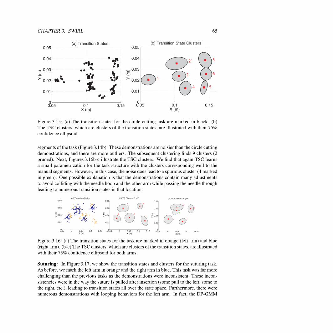
CHAPTER 3. SWIRL 65
0.05 0.1 0.150
0.01
0.02
0.03
0.04
0.05
X (m)
Y (
m)
(a) Transition States
0.05 0.1 0.150
0.01
0.02
0.03
0.04
0.05
X (m)
Y (
m)
(b) Transition State Clusters
1
2
2’ 3
4 5
6
Figure 3.15: (a) The transition states for the circle cutting task are marked in black. (b)The TSC clusters, which are clusters of the transition states, are illustrated with their 75%confidence ellipsoid.
segments of the task (Figure 3.14b). These demonstrations are noisier than the circle cuttingdemonstrations, and there are more outliers. The subsequent clustering finds 9 clusters (2pruned). Next, Figures 3.16b-c illustrate the TSC clusters. We find that again TSC learnsa small parametrization for the task structure with the clusters corresponding well to themanual segments. However, in this case, the noise does lead to a spurious cluster (4 markedin green). One possible explanation is that the demonstrations contain many adjustmentsto avoid colliding with the needle hoop and the other arm while passing the needle throughleading to numerous transition states in that location.
−0.05 0 0.05 0.1 0.150
0.02
0.04
0.06
0.08(a) Transition States
X (m)
Y (
m)
−0.05 0 0.05 0.1 0.150
0.02
0.04
0.06
0.08
X (m)
Y (
m)
(b) TS Clusters “Left”
−0.05 0 0.05 0.1 0.150
0.02
0.04
0.06
0.08
X (m)
Y (
m)
(c) TS Clusters “Right”
1
2
3
4
5
1
2
4
3
5
Figure 3.16: (a) The transition states for the task are marked in orange (left arm) and blue(right arm). (b-c) The TSC clusters, which are clusters of the transition states, are illustratedwith their 75% confidence ellipsoid for both arms
Suturing: In Figure 3.17, we show the transition states and clusters for the suturing task.As before, we mark the left arm in orange and the right arm in blue. This task was far morechallenging than the previous tasks as the demonstrations were inconsistent. These incon-sistencies were in the way the suture is pulled after insertion (some pull to the left, some tothe right, etc.), leading to transition states all over the state space. Furthermore, there werenumerous demonstrations with looping behaviors for the left arm. In fact, the DP-GMM
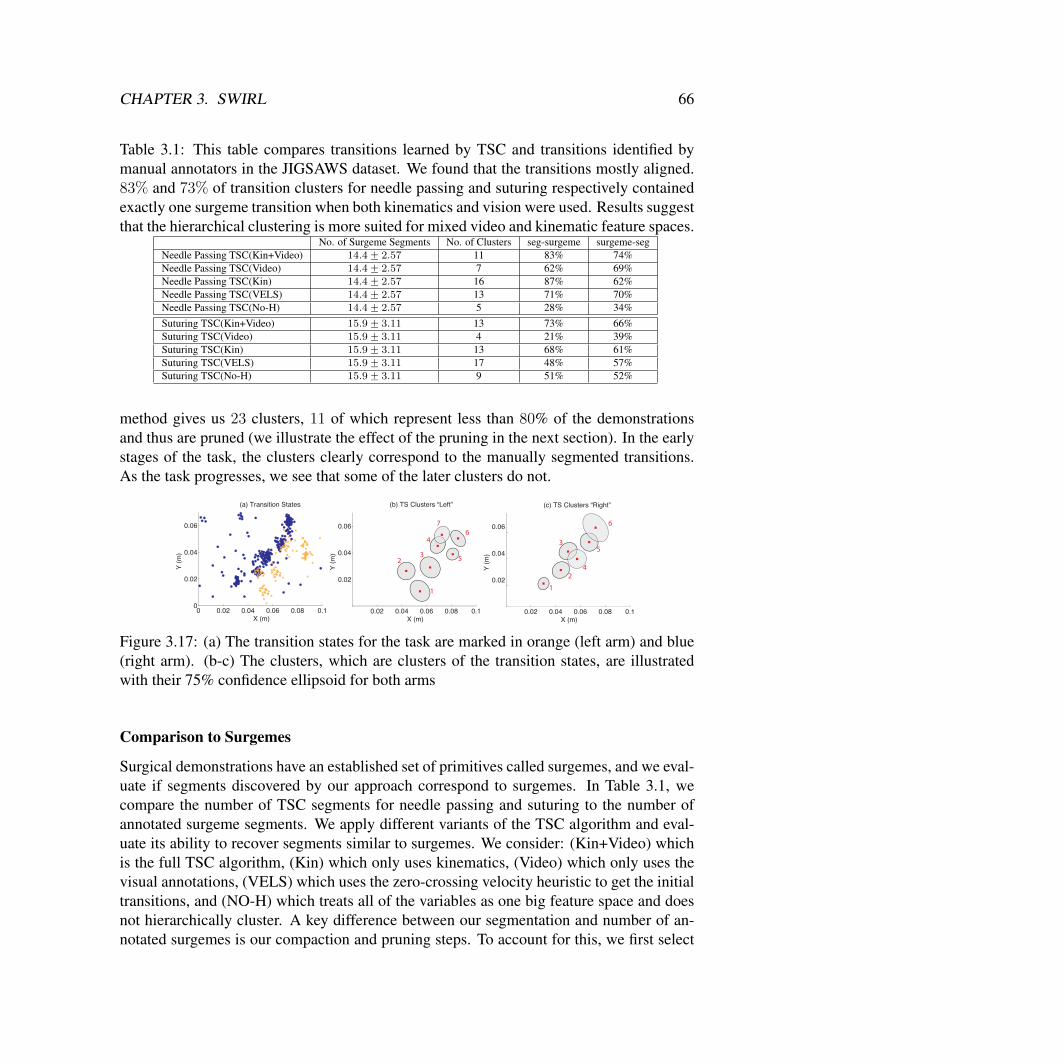
CHAPTER 3. SWIRL 66
Table 3.1: This table compares transitions learned by TSC and transitions identified bymanual annotators in the JIGSAWS dataset. We found that the transitions mostly aligned.83% and 73% of transition clusters for needle passing and suturing respectively containedexactly one surgeme transition when both kinematics and vision were used. Results suggestthat the hierarchical clustering is more suited for mixed video and kinematic feature spaces.
No. of Surgeme Segments No. of Clusters seg-surgeme surgeme-segNeedle Passing TSC(Kin+Video) 14.4˘ 2.57 11 83% 74%Needle Passing TSC(Video) 14.4˘ 2.57 7 62% 69%Needle Passing TSC(Kin) 14.4˘ 2.57 16 87% 62%Needle Passing TSC(VELS) 14.4˘ 2.57 13 71% 70%Needle Passing TSC(No-H) 14.4˘ 2.57 5 28% 34%Suturing TSC(Kin+Video) 15.9˘ 3.11 13 73% 66%Suturing TSC(Video) 15.9˘ 3.11 4 21% 39%Suturing TSC(Kin) 15.9˘ 3.11 13 68% 61%Suturing TSC(VELS) 15.9˘ 3.11 17 48% 57%Suturing TSC(No-H) 15.9˘ 3.11 9 51% 52%
method gives us 23 clusters, 11 of which represent less than 80% of the demonstrationsand thus are pruned (we illustrate the effect of the pruning in the next section). In the earlystages of the task, the clusters clearly correspond to the manually segmented transitions.As the task progresses, we see that some of the later clusters do not.
0 0.02 0.04 0.06 0.08 0.10
0.02
0.04
0.06
(a) Transition States
X (m)
Y (
m)
0.02 0.04 0.06 0.08 0.1
0.02
0.04
0.06
X (m)
Y (
m)
(b) TS Clusters “Left”
0.02 0.04 0.06 0.08 0.1
0.02
0.04
0.06
X (m)
Y (
m)
(c) TS Clusters “Right”
1
23
4
5
7
6
1
2
3
4
5
6
Figure 3.17: (a) The transition states for the task are marked in orange (left arm) and blue(right arm). (b-c) The clusters, which are clusters of the transition states, are illustratedwith their 75% confidence ellipsoid for both arms
Comparison to Surgemes
Surgical demonstrations have an established set of primitives called surgemes, and we eval-uate if segments discovered by our approach correspond to surgemes. In Table 3.1, wecompare the number of TSC segments for needle passing and suturing to the number ofannotated surgeme segments. We apply different variants of the TSC algorithm and eval-uate its ability to recover segments similar to surgemes. We consider: (Kin+Video) whichis the full TSC algorithm, (Kin) which only uses kinematics, (Video) which only uses thevisual annotations, (VELS) which uses the zero-crossing velocity heuristic to get the initialtransitions, and (NO-H) which treats all of the variables as one big feature space and doesnot hierarchically cluster. A key difference between our segmentation and number of an-notated surgemes is our compaction and pruning steps. To account for this, we first select
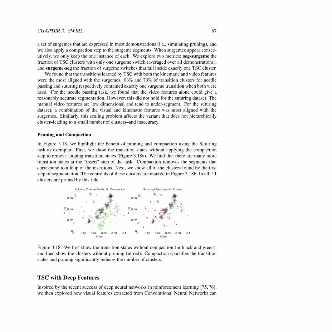
CHAPTER 3. SWIRL 67
a set of surgemes that are expressed in most demonstrations (i.e., simulating pruning), andwe also apply a compaction step to the surgeme segments. When surgemes appear consec-utively, we only keep the one instance of each. We explore two metrics: seg-surgeme thefraction of TSC clusters with only one surgeme switch (averaged over all demonstrations),and surgeme-seg the fraction of surgeme switches that fall inside exactly one TSC cluster.
We found that the transitions learned by TSC with both the kinematic and video featureswere the most aligned with the surgemes. 83% and 73% of transition clusters for needlepassing and suturing respectively contained exactly one surgeme transition when both wereused. For the needle passing task, we found that the video features alone could give areasonably accurate segmentation. However, this did not hold for the suturing dataset. Themanual video features are low dimensional and tend to under-segment. For the suturingdataset, a combination of the visual and kinematic features was most aligned with thesurgemes. Similarly, this scaling problem affects the variant that does not hierarchicallycluster–leading to a small number of clusters–and inaccuracy.
Pruning and Compaction
In Figure 3.18, we highlight the benefit of pruning and compaction using the Suturingtask as exemplar. First, we show the transition states without applying the compactionstep to remove looping transition states (Figure 3.18a). We find that there are many moretransition states at the “insert" step of the task. Compaction removes the segments thatcorrespond to a loop of the insertions. Next, we show all of the clusters found by the firststep of segmentation. The centroids of these clusters are marked in Figure 3.18b. In all, 11clusters are pruned by this rule.
0 0.02 0.04 0.06 0.08 0.10
0.02
0.04
0.06
Suturing Change Points: No Compaction
X (m)
Y (
m)
0 0.02 0.04 0.06 0.08 0.10
0.02
0.04
0.06
Suturing Milestones No Pruning
X (m)
Y (
m)
Figure 3.18: We first show the transition states without compaction (in black and green),and then show the clusters without pruning (in red). Compaction sparsifies the transitionstates and pruning significantly reduces the number of clusters.
TSC with Deep FeaturesInspired by the recent success of deep neural networks in reinforcement learning [75, 76],we then explored how visual features extracted from Convolutional Neural Networks can
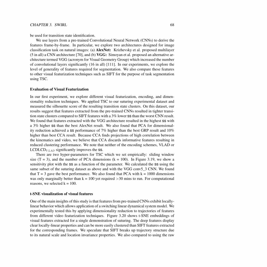
CHAPTER 3. SWIRL 68
be used for transition state identification.We use layers from a pre-trained Convolutional Neural Network (CNNs) to derive the
features frame-by-frame. In particular, we explore two architectures designed for imageclassification task on natural images: (a) AlexNet: Krizhevsky et al. proposed multilayer(5 in all) a CNN architecture [70], and (b) VGG: Simoyan et al. proposed an alternative ar-chitecture termed VGG (acronym for Visual Geometry Group) which increased the numberof convolutional layers significantly (16 in all) [111]. In our experiments, we explore thelevel of generality of features required for segmentation. We also compare these featuresto other visual featurization techniques such as SIFT for the purpose of task segmentationusing TSC.
Evaluation of Visual Featurization
In our first experiment, we explore different visual featurization, encoding, and dimen-sionality reduction techniques. We applied TSC to our suturing experimental dataset andmeasured the silhouette score of the resulting transition state clusters. On this dataset, ourresults suggest that features extracted from the pre-trained CNNs resulted in tighter transi-tion state clusters compared to SIFT features with a 3% lower ss than the worst CNN result.We found that features extracted with the VGG architecture resulted in the highest ss witha 3% higher ss than the best AlexNet result. We also found that PCA for dimensional-ity reduction achieved a ss performance of 7% higher than the best GRP result and 10%higher than best CCA result. Because CCA finds projections of high correlation betweenthe kinematics and video, we believe that CCA discards informative features resulting inreduced clustering performance. We note that neither of the encoding schemes, VLAD orLCDLCDV LAD significantly improves the ss.
There are two hyper-parameters for TSC which we set empirically: sliding windowsize (T = 3), and the number of PCA dimensions (k = 100). In Figure 3.19, we show asensitivity plot with the ss as a function of the parameter. We calculated the ss using thesame subset of the suturing dataset as above and with the VGG conv5_3 CNN. We foundthat T = 3 gave the best performance. We also found that PCA with k = 1000 dimensionswas only marginally better than k = 100 yet required ą30 mins to run. For computationalreasons, we selected k = 100.
t-SNE visualization of visual features
One of the main insights of this study is that features from pre-trained CNNs exhibit locally-linear behavior which allows application of a switching linear dynamical system model. Weexperimentally tested this by applying dimensionality reduction to trajectories of featuresfrom different video featurization techniques. Figure 3.20 shows t-SNE embeddings ofvisual features extracted for a single demonstration of suturing. The deep features displayclear locally-linear properties and can be more easily clustered than SIFT features extractedfor the corresponding frames. We speculate that SIFT breaks up trajectory structure dueto its natural scale and location invariance properties. We also compared to using the raw
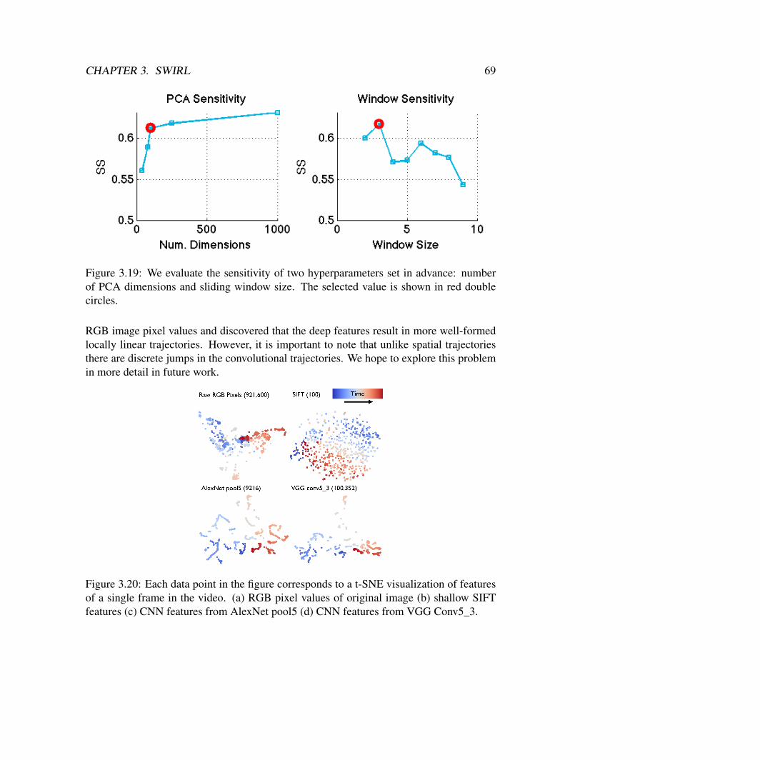
CHAPTER 3. SWIRL 69
Figure 3.19: We evaluate the sensitivity of two hyperparameters set in advance: numberof PCA dimensions and sliding window size. The selected value is shown in red doublecircles.
RGB image pixel values and discovered that the deep features result in more well-formedlocally linear trajectories. However, it is important to note that unlike spatial trajectoriesthere are discrete jumps in the convolutional trajectories. We hope to explore this problemin more detail in future work.
Figure 3.20: Each data point in the figure corresponds to a t-SNE visualization of featuresof a single frame in the video. (a) RGB pixel values of original image (b) shallow SIFTfeatures (c) CNN features from AlexNet pool5 (d) CNN features from VGG Conv5_3.
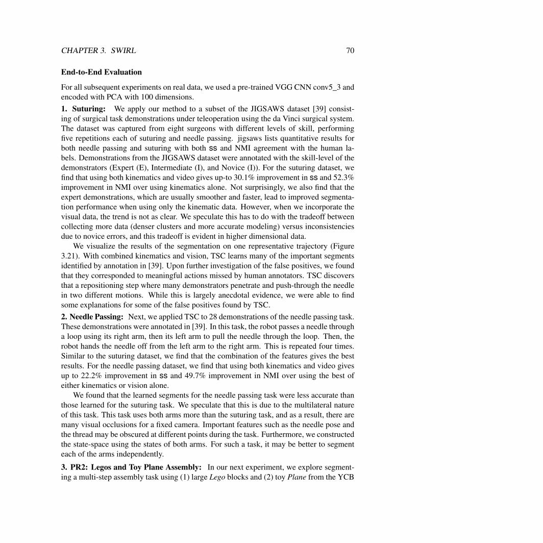
CHAPTER 3. SWIRL 70
End-to-End Evaluation
For all subsequent experiments on real data, we used a pre-trained VGG CNN conv5_3 andencoded with PCA with 100 dimensions.1. Suturing: We apply our method to a subset of the JIGSAWS dataset [39] consist-ing of surgical task demonstrations under teleoperation using the da Vinci surgical system.The dataset was captured from eight surgeons with different levels of skill, performingfive repetitions each of suturing and needle passing. jigsaws lists quantitative results forboth needle passing and suturing with both ss and NMI agreement with the human la-bels. Demonstrations from the JIGSAWS dataset were annotated with the skill-level of thedemonstrators (Expert (E), Intermediate (I), and Novice (I)). For the suturing dataset, wefind that using both kinematics and video gives up-to 30.1% improvement in ss and 52.3%improvement in NMI over using kinematics alone. Not surprisingly, we also find that theexpert demonstrations, which are usually smoother and faster, lead to improved segmenta-tion performance when using only the kinematic data. However, when we incorporate thevisual data, the trend is not as clear. We speculate this has to do with the tradeoff betweencollecting more data (denser clusters and more accurate modeling) versus inconsistenciesdue to novice errors, and this tradeoff is evident in higher dimensional data.
We visualize the results of the segmentation on one representative trajectory (Figure3.21). With combined kinematics and vision, TSC learns many of the important segmentsidentified by annotation in [39]. Upon further investigation of the false positives, we foundthat they corresponded to meaningful actions missed by human annotators. TSC discoversthat a repositioning step where many demonstrators penetrate and push-through the needlein two different motions. While this is largely anecdotal evidence, we were able to findsome explanations for some of the false positives found by TSC.2. Needle Passing: Next, we applied TSC to 28 demonstrations of the needle passing task.These demonstrations were annotated in [39]. In this task, the robot passes a needle througha loop using its right arm, then its left arm to pull the needle through the loop. Then, therobot hands the needle off from the left arm to the right arm. This is repeated four times.Similar to the suturing dataset, we find that the combination of the features gives the bestresults. For the needle passing dataset, we find that using both kinematics and video givesup to 22.2% improvement in ss and 49.7% improvement in NMI over using the best ofeither kinematics or vision alone.
We found that the learned segments for the needle passing task were less accurate thanthose learned for the suturing task. We speculate that this is due to the multilateral natureof this task. This task uses both arms more than the suturing task, and as a result, there aremany visual occlusions for a fixed camera. Important features such as the needle pose andthe thread may be obscured at different points during the task. Furthermore, we constructedthe state-space using the states of both arms. For such a task, it may be better to segmenteach of the arms independently.
3. PR2: Legos and Toy Plane Assembly: In our next experiment, we explore segment-ing a multi-step assembly task using (1) large Lego blocks and (2) toy Plane from the YCB
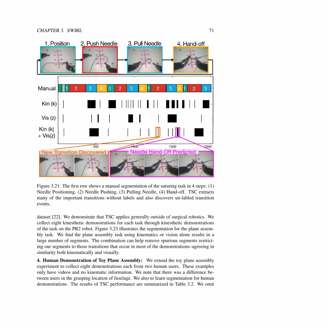
CHAPTER 3. SWIRL 71
Figure 3.21: The first row shows a manual segmentation of the suturing task in 4 steps: (1)Needle Positioning, (2) Needle Pushing, (3) Pulling Needle, (4) Hand-off. TSC extractsmany of the important transitions without labels and also discovers un-labled transitionevents.
dataset [22]. We demonstrate that TSC applies generally outside of surgical robotics. Wecollect eight kinesthetic demonstrations for each task through kinesthetic demonstrationsof the task on the PR2 robot. Figure 3.23 illustrates the segmentation for the plane assem-bly task. We find the plane assembly task using kinematics or vision alone results in alarge number of segments. The combination can help remove spurious segments restrict-ing our segments to those transitions that occur in most of the demonstrations–agreeing insimilarity both kinematically and visually.
4. Human Demonstration of Toy Plane Assembly: We extend the toy plane assemblyexperiment to collect eight demonstrations each from two human users. These examplesonly have videos and no kinematic information. We note that there was a difference be-tween users in the grasping location of fuselage. We also to learn segmentation for humandemonstrations. The results of TSC performance are summarized in Table 3.2. We omit
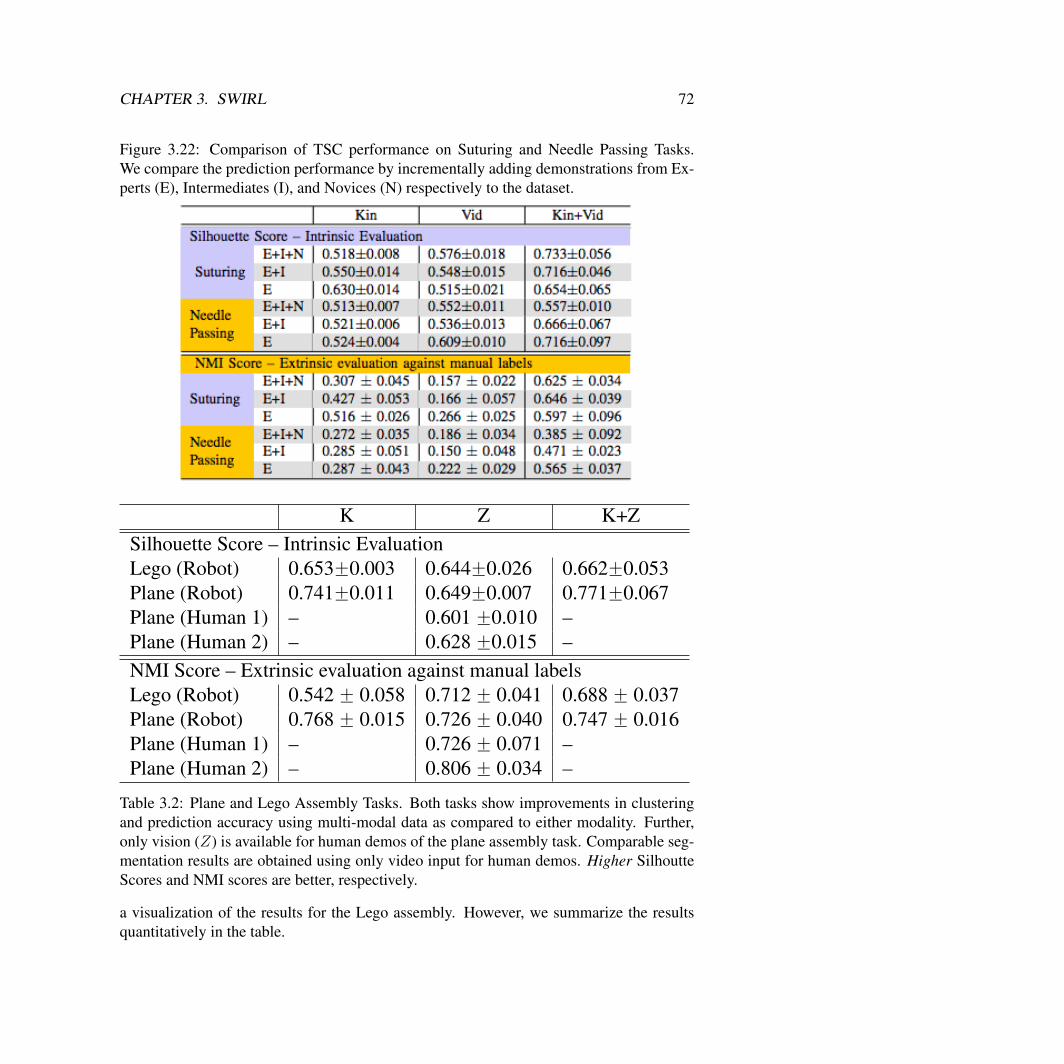
CHAPTER 3. SWIRL 72
Figure 3.22: Comparison of TSC performance on Suturing and Needle Passing Tasks.We compare the prediction performance by incrementally adding demonstrations from Ex-perts (E), Intermediates (I), and Novices (N) respectively to the dataset.
K Z K+ZSilhouette Score – Intrinsic EvaluationLego (Robot) 0.653˘0.003 0.644˘0.026 0.662˘0.053Plane (Robot) 0.741˘0.011 0.649˘0.007 0.771˘0.067Plane (Human 1) – 0.601 ˘0.010 –Plane (Human 2) – 0.628 ˘0.015 –NMI Score – Extrinsic evaluation against manual labelsLego (Robot) 0.542 ˘ 0.058 0.712 ˘ 0.041 0.688 ˘ 0.037Plane (Robot) 0.768 ˘ 0.015 0.726 ˘ 0.040 0.747 ˘ 0.016Plane (Human 1) – 0.726 ˘ 0.071 –Plane (Human 2) – 0.806 ˘ 0.034 –
Table 3.2: Plane and Lego Assembly Tasks. Both tasks show improvements in clusteringand prediction accuracy using multi-modal data as compared to either modality. Further,only vision (Z) is available for human demos of the plane assembly task. Comparable seg-mentation results are obtained using only video input for human demos. Higher SilhoutteScores and NMI scores are better, respectively.
a visualization of the results for the Lego assembly. However, we summarize the resultsquantitatively in the table.
CHAPTER 3. SWIRL 73
Figure 3.23: We compare TSC on 12 kinesthetic demonstrations (top) and 8 human demon-strations (bottom). No kinematics were available for the human demonstrations. We illus-trate the segmentation for an example demonstration of each. Our manual annotation of thetask has five steps and TSC recovers this structure separately for both Kinesthetic demoson PR2 and Human demos with the same visual features.
3.2 SWIRL: Learning With Transition StatesNext, we build on TSC to construct a planner that leverages the structure learned by TSC.Real-world tasks often naturally decompose into a sequence of simpler, locally-solvablesub-tasks. For example, an assembly task might decompose into completing the part’s con-stituent sub-assemblies or a surgical task might decompose into a sequence of movementprimitives. Such structure imposes a strong prior on the class of successful policies andcan focus exploration in reinforcement learning. It reduces the effective time horizon oflearning to the start of the next subtask rather than until task completion. We apply a clus-tering algorithm to identify a latent set of state-space subgoals that sequentially compose toform the global task. This leads to a novel policy search algorithm, called Sequential Win-dowed Inverse Reinforcement Learning (SWIRL), where the demonstrations can bootstrapa self-supervised Q-learning algorithm.
CHAPTER 3. SWIRL 74
Transitions are defined as significant changes in the state trajectory. These transitionscan be spatially and temporally clustered to identify if there are common conditions thattrigger a change in motion across demonstrations. SWIRL extends this basic model with anInverse Reinforcement Learning step that extracts subgoals and computes local cost func-tions from the learned clusters. Learning a policy over the segmented task is nontrivialbecause solving k independent problems neglects any shared structure in the value func-tion during the policy learning phase (e.g., a common failure state). Jointly learning overall segments introduces a dependence on history, namely, any policy must complete stepi before step i ` 1. Learning a memory-dependent policy could lead to an exponentialoverhead of additional states. We show that the problem can be posed as a proper MDP ina lifted state-space that includes an indicator variable of the highest-index t1, ..., ku transi-tion region that has been reached so far if there are Markovian regularity assumptions onthe clustering algorithm.
Model and NotationDirectly optimizing the reward function R in the MDP from the previous section mightbe very challenging. We propose to approximate R with a sequence of smoother rewardfunctions.
Definition 4 (Proxy Task) A proxy task is a set of k MDPs with the same state set, actionset, and dynamics. Associated with each MDP i is a reward function Ri : S ˆ A ÞÑ R.Additionally, associated with each Ri is a transition region ρi Ď S, which is a subset ofthe state-space. A robot accumulates a reward Ri until it reaches the transition ρi, thenthe robot switches to the next reward and transition pair. This process continues until ρk isreached.
A robot is deemed successful when all of the ρi are reached in sequence within a globaltime-horizon T . SWIRL uses a set of initial supervisor demonstrations to construct a proxytask that approximates the original MDP. To make this problem computationally tractable,we make some modeling assumptions.
Modeling Assumption 1. Successful Demonstrations: We need conditions on thedemonstrations to be able to infer the sequential structure. We assume that all demon-strations are successful, that is, they visit each ρi in the same sequence.
Modeling Assumption 2. Quadratic Rewards: We assume that each reward functionRi can be expressed as a quadratic of the form ´ps ´ s0q
TΨps ´ s0q for some positivesemi-definite Ψ and a center point s0 with sT0 Ψs0 “ 0.
Modeling Assumption 3. Ellipsoidal Approximation: Finally, we assume that the tran-sition regions in ρi can be approximated by a set of disjoint ellipsoids.

CHAPTER 3. SWIRL 75
Algorithm Overview
SWIRL can be described in terms of three sub-algorithms:
Inputs: Demonstrations D
1. Sequence Learning: Given D, SWIRL applies TSC to partition the task into ksub-tasks whose start and end are defined by arrival at a sequence of transitions G “rρ1, ..., ρks.
2. Reward Learning: GivenG andD, SWIRL associates a local reward function witheach segment resulting in a sequence of rewards Rseq “ rR1, ..., Rks.
3. Policy Learning: Given Rseq and G, SWIRL applies reinforcement learning tooptimize a policy for the task π.
Outputs: Policy π
In principle, one could couple steps 1 and 2 similar to the results in [97]. We separatethese steps since that allows us to use a different set of features for segmentation than usedfor reward learning. Perceptual features can provide a valuable signal for segmentation butquadratic reward functions may not be meaningful in all perceptual feature spaces.
Sequence Learning Algorithm
First, SWIRL applies a clustering algorithm to the initial demonstrations to learn the transi-tion regions. The clustering model is based on our prior work on Transition State Clustering(TSC) [67, 86]. Transitions are defined as significant changes in the state trajectory. Thesetransitions can be spatially and temporally clustered to identify if there are common condi-tions that trigger a change in motion across demonstrations.
Reward Learning AlgorithmAfter the sequence learning phase, each demonstration is partitioned into k segments. Thereward learning phase uses the learned rρ1, ..., ρks to construct the local rewards rR1, ..., Rks
for the task. Each Ri is a quadratic cost parametrized by a positive semi-definite matrix Ψ.The role of the reward function is to guide the robot to the next transition region ρi. A
first approach is for each segment i, we can define a reward function as follows:
Ripsq “ ´}s´ µi}22,
which is just the Euclidean distance to the centroid.A problem with using Euclidean distance directly is that it uniformly penalizes dis-
agreement with µ in all dimensions. During different stages of a task, some directions willlikely naturally vary more than others. To account for this, we can derive :
Ψrj, ls “ Σ´1,
CHAPTER 3. SWIRL 76
Algorithm 3 Reward InferenceInput: Demonstration D and sub-goals rρ1, ..., ρksSegment each demonstration di into k sub-sequences where the jth is denoted by dirjs.Apply Equation 2 to each set of sub-sequences 1...k.Return: Rseq
which is the inverse of the covariance matrix of all of the state vectors in the segment:
Ψ “ p
endÿ
t“start
ssT q´1, (2)
which is a p ˆ p matrix defined as the covariance of all of the states in the segment i ´ 1to i. Intuitively, if a feature has low variance during this segment, deviation in that featurefrom the desired target it gets penalized. This is exactly the Mahalonabis distance to thenext transition.
For example, suppose one of the features j measures the distance to a reference trajec-tory ut. Further, suppose in step one of the task the demonstrator’s actions are perfectlycorrelated with the trajectory (Ψirj, js is low where variance is in the distance) and in steptwo the actions are uncorrelated with the reference trajectory (Ψirj, js is high). Thus, Ψwill respectively penalize deviation from µirjs more in step one than in step two.
Policy Learningpolicy-learning SWIRL uses the learned transitions rρ1, ..., ρks and Rseq to construct aproxy task to solve via Reinforcement Learning. In this section, we describe learning a pol-icy π given rewards Rseq and an ordered sequence of transitions G. However, this problemis not trivial since solving k independent problems neglects potential shared value structurebetween the local problems (e.g., a common failure state). Furthermore, simply taking theaggregate of the rewards can lead to inconsistencies since there is nothing enforcing theorder of operations. We show that a single policy can be learned jointly over all segmentsover a modified problem where the state-space with additional variables that keep track ofthe previously achieved segments. We present a Q-Learning algorithm [85, 121] that cap-tures the coupling noted above between task segments. In principle, similar techniques canbe used for any other policy search method.
Jointly Learning Over All Segments
In our sequential task definition, we cannot transition to reward Ri`1 unless all previoustransition regions ρ1, ...ρi are reached in sequence. We can leverage the definition of theMarkov Segmentation function formalized earlier to jointly learn across all segments, whileleveraging the segmented structure. We know that the reward transitions (Ri to Ri`1) onlydepend on an arrival at the transition state ρi and not any other aspect of the history. There-fore, we can store an index v, that indicates whether a transition state i P 0, ..., k has been
CHAPTER 3. SWIRL 77
reached. This index can be efficiently incremented when the current state s P ρi`1. Theresult is an augmented state-space
`
sv
˘
to account for previous progress. In this lifted space,the problem is a fully observed MDP. Then, the additional complexity of representing thereward with history over S ˆ rks is only Opkq instead of exponential in the time horizon.
Segmented Q-Learning
At a high-level, the objective of standard Q-Learning is to learn the function Qps, aq of theoptimal policy, which is the expected reward the agent will receive taking action a in states, assuming future behavior is optimal. Q-Learning works by first initializing a random Qfunction. Then, it samples rollouts from an exploration policy collecting ps, a, r, s1q tuples.From these tuples, one can calculate the following value:
yi “ Rps, aq ` arg maxaQps1, aq
Each of the yi can be used to define a loss function since if Q were the true Q function,then the following recurrence would hold:
Qps, aq “ Rps, aq ` arg maxaQps1, aq
So, Q-Learning defines a loss:
LpQq “ÿ
i
}yi ´Qps, aq}22
This loss can be optimized with gradient descent. When the state and action space is dis-crete, the representation of the Q function is a table, and we get the familiar Q-Learning al-gorithm [121]–where each gradient step updates the table with the appropriate value. WhenQ function needs to be approximated, then we get the Deep Q Network algorithm [85].
SWIRL applies a variant of Q-Learning to optimize the policy over the sequential re-wards. The basic change to the algorithm is to augment the state-space with indicator vectorthat indicates the transition regions that have been reached. So each of the rollouts, nowrecords a tuple ps, v, a, r, s1, v’q that additionally stores this information. The Q functionis now defined over states, actions, and segment index–which also selects the appropriatelocal reward function:
Qps, a, vq “ Rvps, aq ` arg maxaQps1, a, v1q
We also need to define an exploration policy, i.e., a stochastic policy with which we willcollect rollouts. To initialize the Q-Learning, we apply Behavioral Cloning locally for eachof the segments to get a policy πi. We apply an ε-greedy version of these policies to collectrollouts.

CHAPTER 3. SWIRL 78
Simulated ExperimentsWe constructed a parallel parking scenario for a robot car with non-holonomic dynamicsand two obstacles (Figure 3.24a), and we also experimented on the standard acrobot domain(Figure 3.24b).
Experimental Methodology
First, we overview our basic experimental methodology. We evaluate SWIRL on two sim-ulated RL benchmarks and two deformable manipulation tasks on the da Vinci surgicalrobot [57]. In all of these tasks, there is a single MDP of interest where the reward is sparse(for a substantial amount of the state-space the reward is zero). The goal of SWIRL is toimprove convergence on this task.
Supervision
In both of the RL benchmarks, the reward function defines a target configuration of therobot. We generated the initial demonstrations using an RRT* motion planner (assumingdeterministic dynamics) [55]. As both the RL benchmarks are stochastic in nature, we usedan MPC-style re-planning approach to control the robot to the target region. On the physicalexperiments, we provided the robot with demonstrations collected in tele-operation. Wecollected fully observed trajectories with both states and actions.
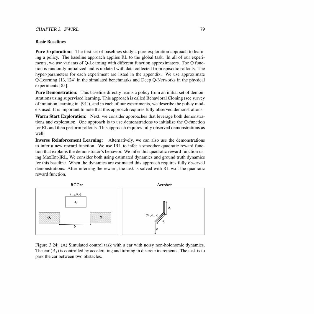
CHAPTER 3. SWIRL 79
Basic Baselines
Pure Exploration: The first set of baselines study a pure exploration approach to learn-ing a policy. The baseline approach applies RL to the global task. In all of our experi-ments, we use variants of Q-Learning with different function approximators. The Q func-tion is randomly initialized and is updated with data collected from episodic rollouts. Thehyper-parameters for each experiment are listed in the appendix. We use approximateQ-Learning [13, 124] in the simulated benchmarks and Deep Q-Networks in the physicalexperiments [85].Pure Demonstration: This baseline directly learns a policy from an initial set of demon-strations using supervised learning. This approach is called Behavioral Cloning (see surveyof imitation learning in [91]), and in each of our experiments, we describe the policy mod-els used. It is important to note that this approach requires fully observed demonstrations.Warm Start Exploration: Next, we consider approaches that leverage both demonstra-tions and exploration. One approach is to use demonstrations to initialize the Q-functionfor RL and then perform rollouts. This approach requires fully observed demonstrations aswell.Inverse Reinforcement Learning: Alternatively, we can also use the demonstrationsto infer a new reward function. We use IRL to infer a smoother quadratic reward func-tion that explains the demonstrator’s behavior. We infer this quadratic reward function us-ing MaxEnt-IRL. We consider both using estimated dynamics and ground truth dynamicsfor this baseline. When the dynamics are estimated this approach requires fully observeddemonstrations. After inferring the reward, the task is solved with RL w.r.t the quadraticreward function.
Figure 3.24: (A) Simulated control task with a car with noisy non-holonomic dynamics.The car (A1) is controlled by accelerating and turning in discrete increments. The task is topark the car between two obstacles.
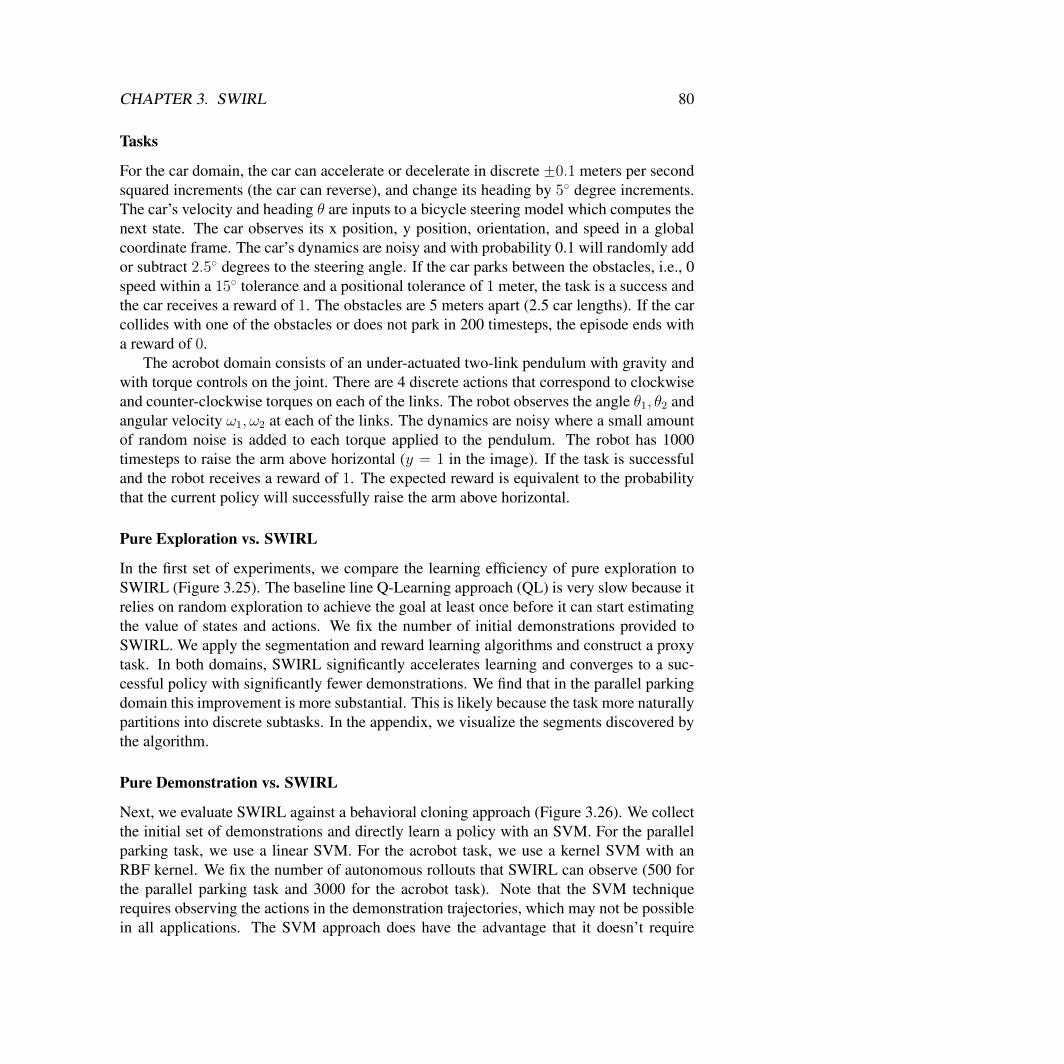
CHAPTER 3. SWIRL 80
Tasks
For the car domain, the car can accelerate or decelerate in discrete ˘0.1 meters per secondsquared increments (the car can reverse), and change its heading by 5˝ degree increments.The car’s velocity and heading θ are inputs to a bicycle steering model which computes thenext state. The car observes its x position, y position, orientation, and speed in a globalcoordinate frame. The car’s dynamics are noisy and with probability 0.1 will randomly addor subtract 2.5˝ degrees to the steering angle. If the car parks between the obstacles, i.e., 0speed within a 15˝ tolerance and a positional tolerance of 1 meter, the task is a success andthe car receives a reward of 1. The obstacles are 5 meters apart (2.5 car lengths). If the carcollides with one of the obstacles or does not park in 200 timesteps, the episode ends witha reward of 0.
The acrobot domain consists of an under-actuated two-link pendulum with gravity andwith torque controls on the joint. There are 4 discrete actions that correspond to clockwiseand counter-clockwise torques on each of the links. The robot observes the angle θ1, θ2 andangular velocity ω1, ω2 at each of the links. The dynamics are noisy where a small amountof random noise is added to each torque applied to the pendulum. The robot has 1000timesteps to raise the arm above horizontal (y “ 1 in the image). If the task is successfuland the robot receives a reward of 1. The expected reward is equivalent to the probabilitythat the current policy will successfully raise the arm above horizontal.
Pure Exploration vs. SWIRL
In the first set of experiments, we compare the learning efficiency of pure exploration toSWIRL (Figure 3.25). The baseline line Q-Learning approach (QL) is very slow because itrelies on random exploration to achieve the goal at least once before it can start estimatingthe value of states and actions. We fix the number of initial demonstrations provided toSWIRL. We apply the segmentation and reward learning algorithms and construct a proxytask. In both domains, SWIRL significantly accelerates learning and converges to a suc-cessful policy with significantly fewer demonstrations. We find that in the parallel parkingdomain this improvement is more substantial. This is likely because the task more naturallypartitions into discrete subtasks. In the appendix, we visualize the segments discovered bythe algorithm.
Pure Demonstration vs. SWIRL
Next, we evaluate SWIRL against a behavioral cloning approach (Figure 3.26). We collectthe initial set of demonstrations and directly learn a policy with an SVM. For the parallelparking task, we use a linear SVM. For the acrobot task, we use a kernel SVM with anRBF kernel. We fix the number of autonomous rollouts that SWIRL can observe (500 forthe parallel parking task and 3000 for the acrobot task). Note that the SVM techniquerequires observing the actions in the demonstration trajectories, which may not be possiblein all applications. The SVM approach does have the advantage that it doesn’t require
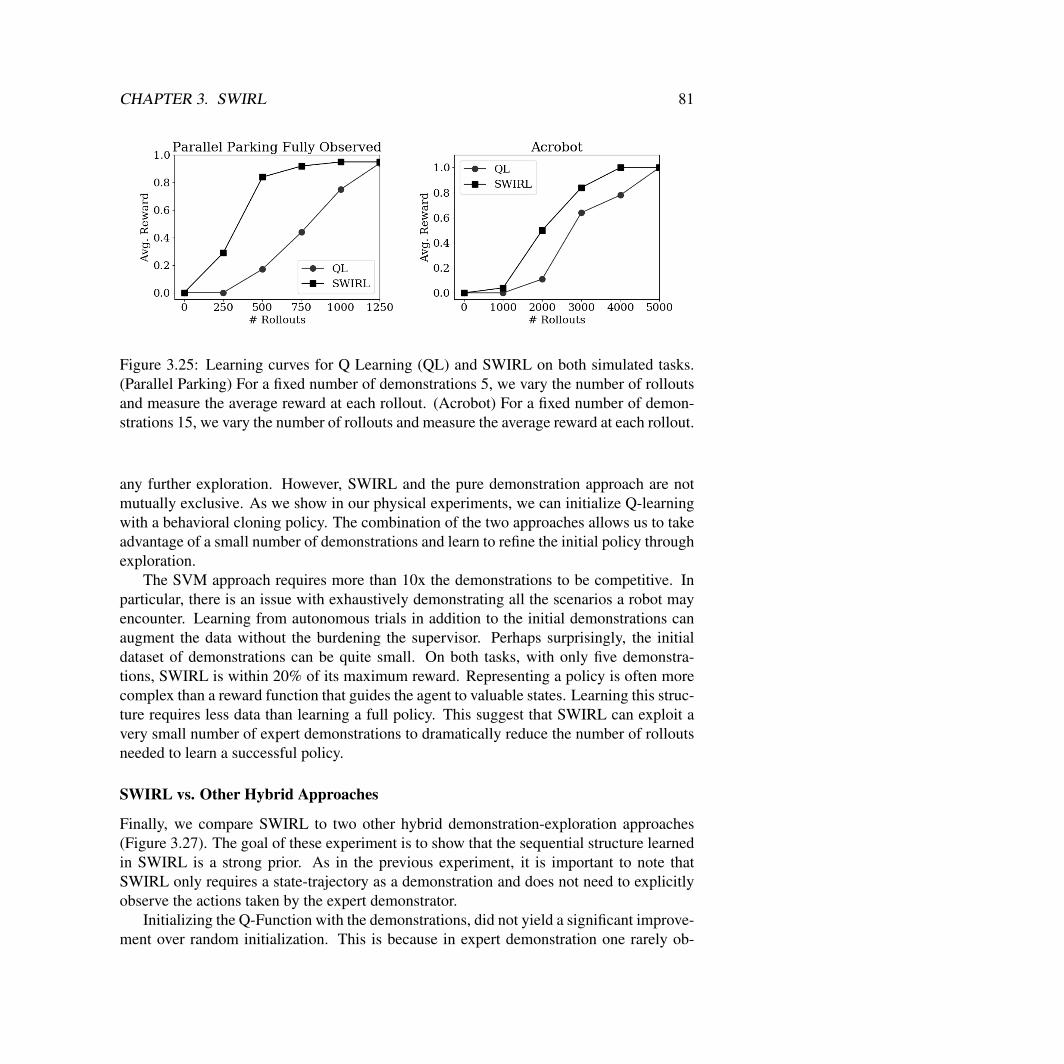
CHAPTER 3. SWIRL 81
Figure 3.25: Learning curves for Q Learning (QL) and SWIRL on both simulated tasks.(Parallel Parking) For a fixed number of demonstrations 5, we vary the number of rolloutsand measure the average reward at each rollout. (Acrobot) For a fixed number of demon-strations 15, we vary the number of rollouts and measure the average reward at each rollout.
any further exploration. However, SWIRL and the pure demonstration approach are notmutually exclusive. As we show in our physical experiments, we can initialize Q-learningwith a behavioral cloning policy. The combination of the two approaches allows us to takeadvantage of a small number of demonstrations and learn to refine the initial policy throughexploration.
The SVM approach requires more than 10x the demonstrations to be competitive. Inparticular, there is an issue with exhaustively demonstrating all the scenarios a robot mayencounter. Learning from autonomous trials in addition to the initial demonstrations canaugment the data without the burdening the supervisor. Perhaps surprisingly, the initialdataset of demonstrations can be quite small. On both tasks, with only five demonstra-tions, SWIRL is within 20% of its maximum reward. Representing a policy is often morecomplex than a reward function that guides the agent to valuable states. Learning this struc-ture requires less data than learning a full policy. This suggest that SWIRL can exploit avery small number of expert demonstrations to dramatically reduce the number of rolloutsneeded to learn a successful policy.
SWIRL vs. Other Hybrid Approaches
Finally, we compare SWIRL to two other hybrid demonstration-exploration approaches(Figure 3.27). The goal of these experiment is to show that the sequential structure learnedin SWIRL is a strong prior. As in the previous experiment, it is important to note thatSWIRL only requires a state-trajectory as a demonstration and does not need to explicitlyobserve the actions taken by the expert demonstrator.
Initializing the Q-Function with the demonstrations, did not yield a significant improve-ment over random initialization. This is because in expert demonstration one rarely ob-
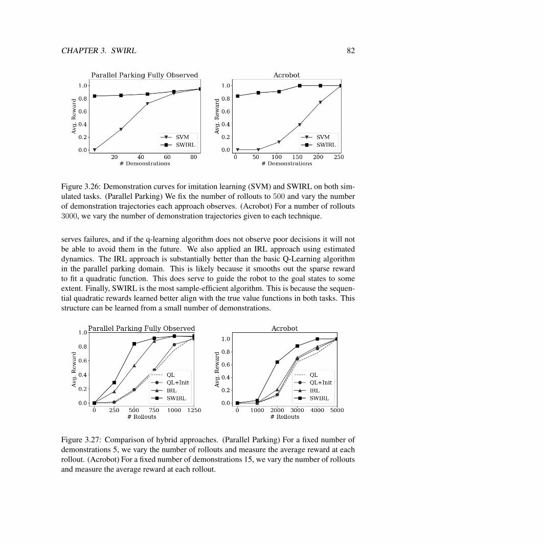
CHAPTER 3. SWIRL 82
Figure 3.26: Demonstration curves for imitation learning (SVM) and SWIRL on both sim-ulated tasks. (Parallel Parking) We fix the number of rollouts to 500 and vary the numberof demonstration trajectories each approach observes. (Acrobot) For a number of rollouts3000, we vary the number of demonstration trajectories given to each technique.
serves failures, and if the q-learning algorithm does not observe poor decisions it will notbe able to avoid them in the future. We also applied an IRL approach using estimateddynamics. The IRL approach is substantially better than the basic Q-Learning algorithmin the parallel parking domain. This is likely because it smooths out the sparse rewardto fit a quadratic function. This does serve to guide the robot to the goal states to someextent. Finally, SWIRL is the most sample-efficient algorithm. This is because the sequen-tial quadratic rewards learned better align with the true value functions in both tasks. Thisstructure can be learned from a small number of demonstrations.
Figure 3.27: Comparison of hybrid approaches. (Parallel Parking) For a fixed number ofdemonstrations 5, we vary the number of rollouts and measure the average reward at eachrollout. (Acrobot) For a fixed number of demonstrations 15, we vary the number of rolloutsand measure the average reward at each rollout.
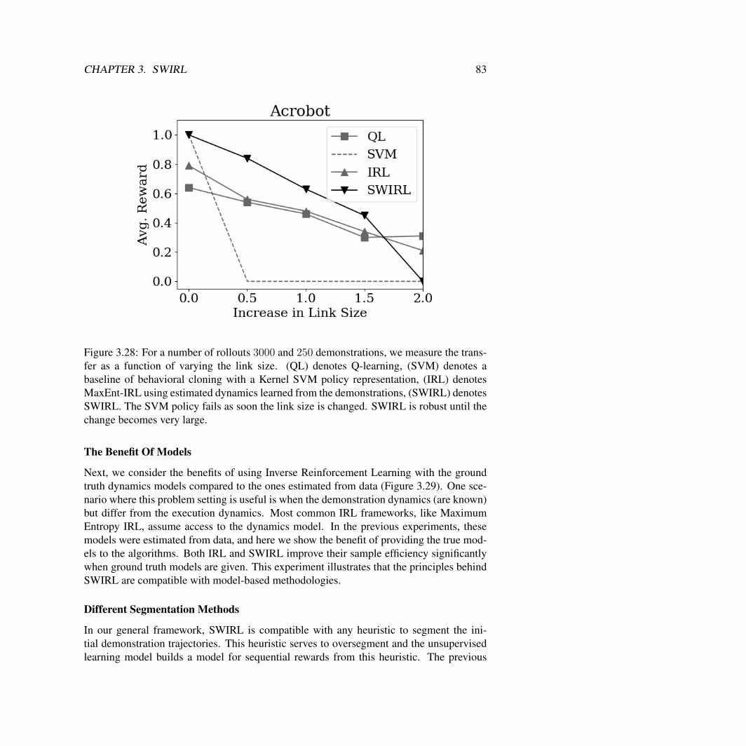
CHAPTER 3. SWIRL 83
Figure 3.28: For a number of rollouts 3000 and 250 demonstrations, we measure the trans-fer as a function of varying the link size. (QL) denotes Q-learning, (SVM) denotes abaseline of behavioral cloning with a Kernel SVM policy representation, (IRL) denotesMaxEnt-IRL using estimated dynamics learned from the demonstrations, (SWIRL) denotesSWIRL. The SVM policy fails as soon the link size is changed. SWIRL is robust until thechange becomes very large.
The Benefit Of Models
Next, we consider the benefits of using Inverse Reinforcement Learning with the groundtruth dynamics models compared to the ones estimated from data (Figure 3.29). One sce-nario where this problem setting is useful is when the demonstration dynamics (are known)but differ from the execution dynamics. Most common IRL frameworks, like MaximumEntropy IRL, assume access to the dynamics model. In the previous experiments, thesemodels were estimated from data, and here we show the benefit of providing the true mod-els to the algorithms. Both IRL and SWIRL improve their sample efficiency significantlywhen ground truth models are given. This experiment illustrates that the principles behindSWIRL are compatible with model-based methodologies.
Different Segmentation Methods
In our general framework, SWIRL is compatible with any heuristic to segment the ini-tial demonstration trajectories. This heuristic serves to oversegment and the unsupervisedlearning model builds a model for sequential rewards from this heuristic. The previous
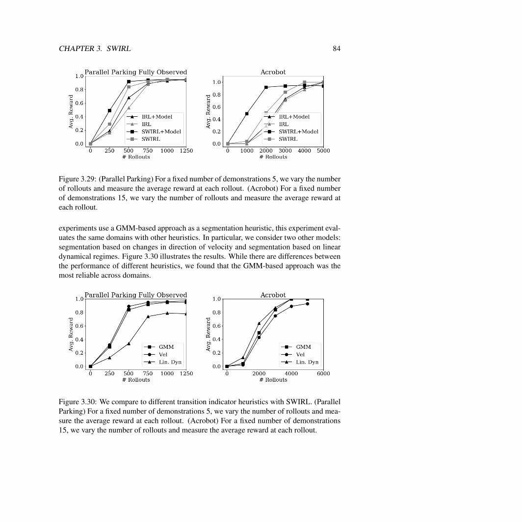
CHAPTER 3. SWIRL 84
Figure 3.29: (Parallel Parking) For a fixed number of demonstrations 5, we vary the numberof rollouts and measure the average reward at each rollout. (Acrobot) For a fixed numberof demonstrations 15, we vary the number of rollouts and measure the average reward ateach rollout.
experiments use a GMM-based approach as a segmentation heuristic, this experiment eval-uates the same domains with other heuristics. In particular, we consider two other models:segmentation based on changes in direction of velocity and segmentation based on lineardynamical regimes. Figure 3.30 illustrates the results. While there are differences betweenthe performance of different heuristics, we found that the GMM-based approach was themost reliable across domains.
Figure 3.30: We compare to different transition indicator heuristics with SWIRL. (ParallelParking) For a fixed number of demonstrations 5, we vary the number of rollouts and mea-sure the average reward at each rollout. (Acrobot) For a fixed number of demonstrations15, we vary the number of rollouts and measure the average reward at each rollout.
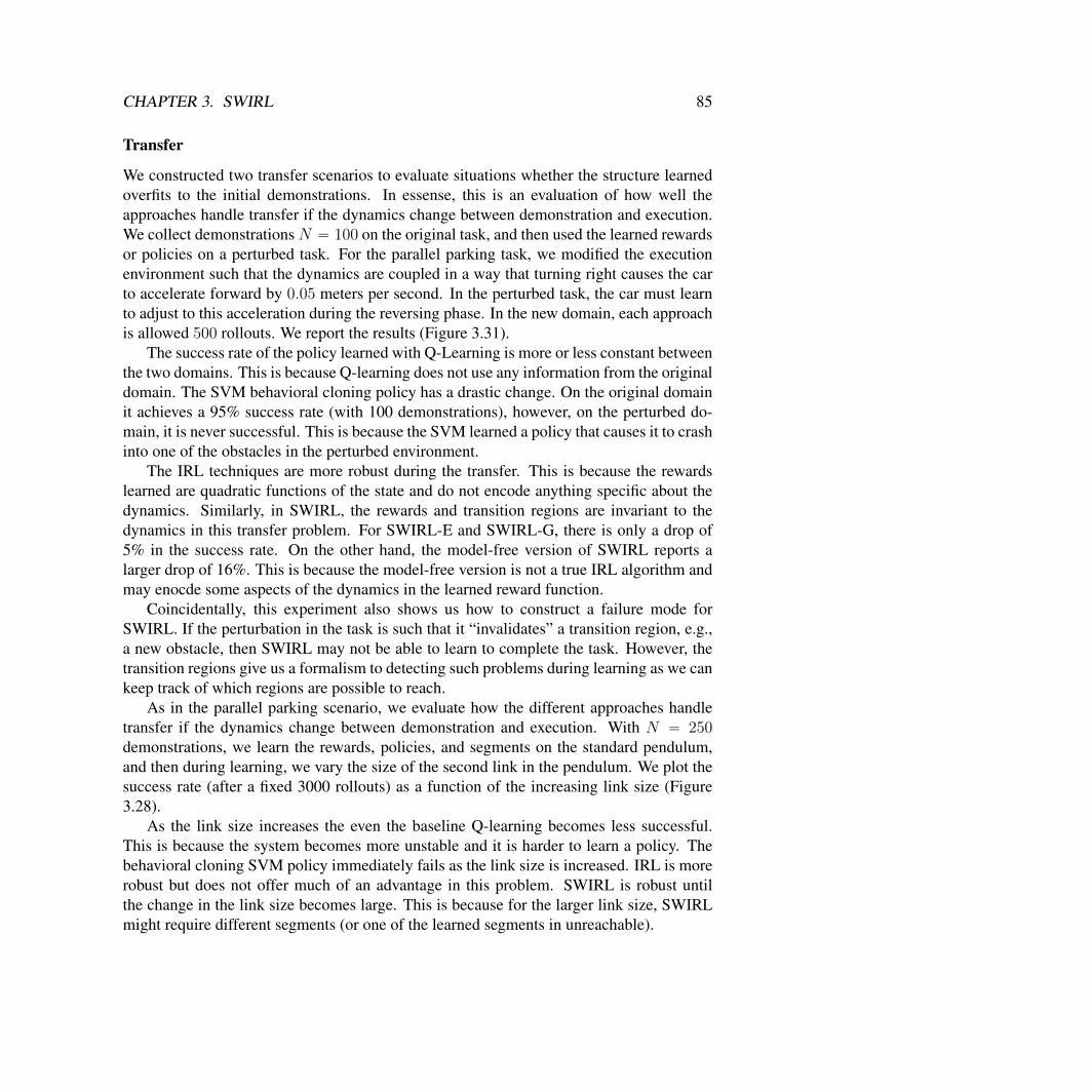
CHAPTER 3. SWIRL 85
Transfer
We constructed two transfer scenarios to evaluate situations whether the structure learnedoverfits to the initial demonstrations. In essense, this is an evaluation of how well theapproaches handle transfer if the dynamics change between demonstration and execution.We collect demonstrations N “ 100 on the original task, and then used the learned rewardsor policies on a perturbed task. For the parallel parking task, we modified the executionenvironment such that the dynamics are coupled in a way that turning right causes the carto accelerate forward by 0.05 meters per second. In the perturbed task, the car must learnto adjust to this acceleration during the reversing phase. In the new domain, each approachis allowed 500 rollouts. We report the results (Figure 3.31).
The success rate of the policy learned with Q-Learning is more or less constant betweenthe two domains. This is because Q-learning does not use any information from the originaldomain. The SVM behavioral cloning policy has a drastic change. On the original domainit achieves a 95% success rate (with 100 demonstrations), however, on the perturbed do-main, it is never successful. This is because the SVM learned a policy that causes it to crashinto one of the obstacles in the perturbed environment.
The IRL techniques are more robust during the transfer. This is because the rewardslearned are quadratic functions of the state and do not encode anything specific about thedynamics. Similarly, in SWIRL, the rewards and transition regions are invariant to thedynamics in this transfer problem. For SWIRL-E and SWIRL-G, there is only a drop of5% in the success rate. On the other hand, the model-free version of SWIRL reports alarger drop of 16%. This is because the model-free version is not a true IRL algorithm andmay enocde some aspects of the dynamics in the learned reward function.
Coincidentally, this experiment also shows us how to construct a failure mode forSWIRL. If the perturbation in the task is such that it “invalidates” a transition region, e.g.,a new obstacle, then SWIRL may not be able to learn to complete the task. However, thetransition regions give us a formalism to detecting such problems during learning as we cankeep track of which regions are possible to reach.
As in the parallel parking scenario, we evaluate how the different approaches handletransfer if the dynamics change between demonstration and execution. With N “ 250demonstrations, we learn the rewards, policies, and segments on the standard pendulum,and then during learning, we vary the size of the second link in the pendulum. We plot thesuccess rate (after a fixed 3000 rollouts) as a function of the increasing link size (Figure3.28).
As the link size increases the even the baseline Q-learning becomes less successful.This is because the system becomes more unstable and it is harder to learn a policy. Thebehavioral cloning SVM policy immediately fails as the link size is increased. IRL is morerobust but does not offer much of an advantage in this problem. SWIRL is robust untilthe change in the link size becomes large. This is because for the larger link size, SWIRLmight require different segments (or one of the learned segments in unreachable).

CHAPTER 3. SWIRL 86
Figure 3.31: For 500 rollouts and 100 demonstrations, we measure the robustness of the ap-proaches to changes in the execution dynamics. (QL) denotes Q-learning, (SVM) denotesa baseline of behavioral cloning with a SVM policy representation, (IRL) denotes MaxEnt-IRL with estimated dynamics, and (SWIRL) denotes the model-free version of SWIRL.While the SVM is 95% successful on the original domain, its success does not transfer tothe perturbed setting. On the other hand, SWIRL learns rewards and segments that transferto the new dynamics since they are state-space goals.
Sensitivity
Next, we evaluated the sensitivity of SWIRL to different initial demonstration sets (Figure3.32). We sampled random initial demonstration sets and re-ran the algorithm on each ofthe two domains 100 times. Figure 3.32 plots the mean reward as a function of the numberof rollouts and 2 standard deviations over all of the trials. We find that SWIRL is not verysensitive to the particular initial demonstration dataset. In fact, the 2 standard deviationerror bar is less than the improvement in convergence in previous experiments.
Segmentation and Partial Observation
Next, we made the Parallel Parking domain more difficult to illustrate the connection be-tween segmentation and memory in RL. We hid the velocity state from the robot, so thecar only sees px, y, θq. As before, if the car collides with one of the obstacle or does notpark in 200 timesteps the episode ends. We call this domain Parallel Parking with PartialObservation (PP-PO).
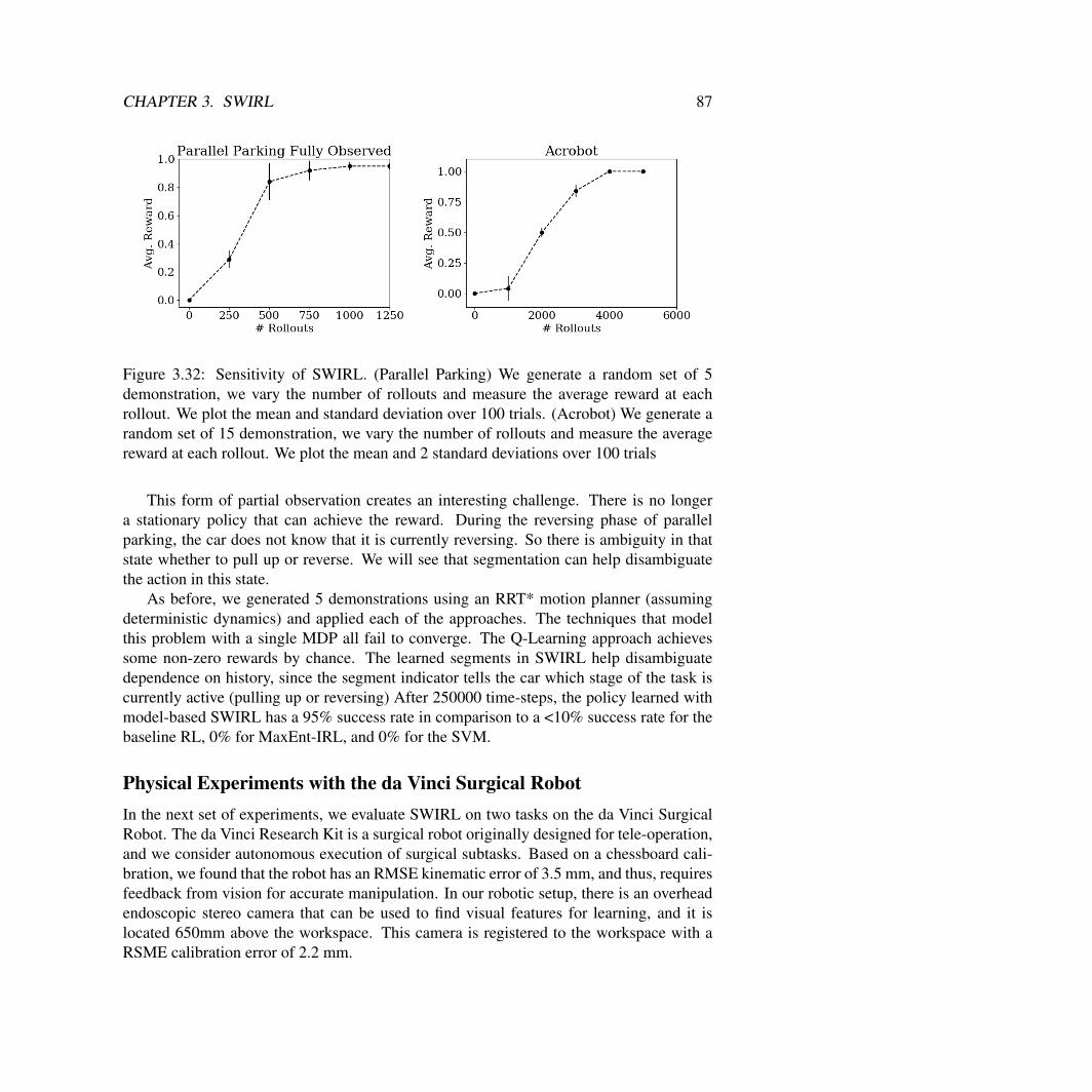
CHAPTER 3. SWIRL 87
Figure 3.32: Sensitivity of SWIRL. (Parallel Parking) We generate a random set of 5demonstration, we vary the number of rollouts and measure the average reward at eachrollout. We plot the mean and standard deviation over 100 trials. (Acrobot) We generate arandom set of 15 demonstration, we vary the number of rollouts and measure the averagereward at each rollout. We plot the mean and 2 standard deviations over 100 trials
This form of partial observation creates an interesting challenge. There is no longera stationary policy that can achieve the reward. During the reversing phase of parallelparking, the car does not know that it is currently reversing. So there is ambiguity in thatstate whether to pull up or reverse. We will see that segmentation can help disambiguatethe action in this state.
As before, we generated 5 demonstrations using an RRT* motion planner (assumingdeterministic dynamics) and applied each of the approaches. The techniques that modelthis problem with a single MDP all fail to converge. The Q-Learning approach achievessome non-zero rewards by chance. The learned segments in SWIRL help disambiguatedependence on history, since the segment indicator tells the car which stage of the task iscurrently active (pulling up or reversing) After 250000 time-steps, the policy learned withmodel-based SWIRL has a 95% success rate in comparison to a <10% success rate for thebaseline RL, 0% for MaxEnt-IRL, and 0% for the SVM.
Physical Experiments with the da Vinci Surgical RobotIn the next set of experiments, we evaluate SWIRL on two tasks on the da Vinci SurgicalRobot. The da Vinci Research Kit is a surgical robot originally designed for tele-operation,and we consider autonomous execution of surgical subtasks. Based on a chessboard cali-bration, we found that the robot has an RMSE kinematic error of 3.5 mm, and thus, requiresfeedback from vision for accurate manipulation. In our robotic setup, there is an overheadendoscopic stereo camera that can be used to find visual features for learning, and it islocated 650mm above the workspace. This camera is registered to the workspace with aRSME calibration error of 2.2 mm.
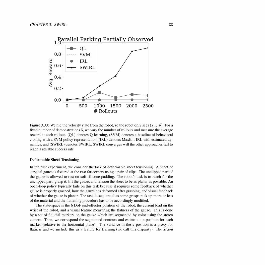
CHAPTER 3. SWIRL 88
Figure 3.33: We hid the velocity state from the robot, so the robot only sees px, y, θq. For afixed number of demonstrations 5, we vary the number of rollouts and measure the averagereward at each rollout. (QL) denotes Q-learning, (SVM) denotes a baseline of behavioralcloning with a SVM policy representation, (IRL) denotes MaxEnt-IRL with estimated dy-namics, and (SWIRL) denotes SWIRL. SWIRL converges will the other approaches fail toreach a reliable success rate
Deformable Sheet Tensioning
In the first experiment, we consider the task of deformable sheet tensioning. A sheet ofsurgical gauze is fixtured at the two far corners using a pair of clips. The unclipped part ofthe gauze is allowed to rest on soft silicone padding. The robot’s task is to reach for theunclipped part, grasp it, lift the gauze, and tension the sheet to be as planar as possible. Anopen-loop policy typically fails on this task because it requires some feedback of whethergauze is properly grasped, how the gauze has deformed after grasping, and visual feedbackof whether the gauze is planar. The task is sequential as some grasps pick up more or lessof the material and the flattening procedure has to be accordingly modified.
The state-space is the 6 DoF end-effector position of the robot, the current load on thewrist of the robot, and a visual feature measuring the flatness of the gauze. This is doneby a set of fiducial markers on the gauze which are segmented by color using the stereocamera. Then, we correspond the segmented contours and estimate a z position for eachmarker (relative to the horizontal plane). The variance in the z position is a proxy forflatness and we include this as a feature for learning (we call this disparity). The action
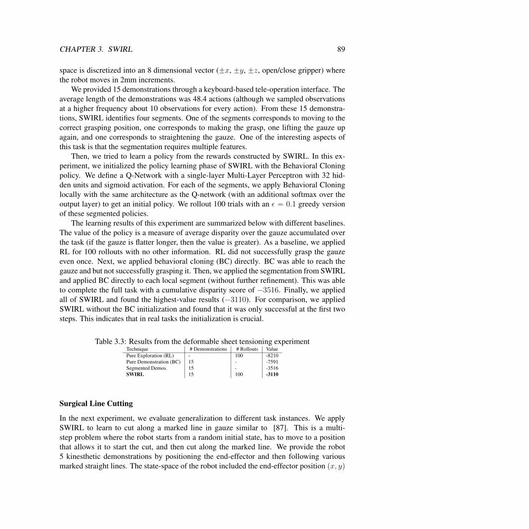
CHAPTER 3. SWIRL 89
space is discretized into an 8 dimensional vector (˘x, ˘y, ˘z, open/close gripper) wherethe robot moves in 2mm increments.
We provided 15 demonstrations through a keyboard-based tele-operation interface. Theaverage length of the demonstrations was 48.4 actions (although we sampled observationsat a higher frequency about 10 observations for every action). From these 15 demonstra-tions, SWIRL identifies four segments. One of the segments corresponds to moving to thecorrect grasping position, one corresponds to making the grasp, one lifting the gauze upagain, and one corresponds to straightening the gauze. One of the interesting aspects ofthis task is that the segmentation requires multiple features.
Then, we tried to learn a policy from the rewards constructed by SWIRL. In this ex-periment, we initialized the policy learning phase of SWIRL with the Behavioral Cloningpolicy. We define a Q-Network with a single-layer Multi-Layer Perceptron with 32 hid-den units and sigmoid activation. For each of the segments, we apply Behavioral Cloninglocally with the same architecture as the Q-network (with an additional softmax over theoutput layer) to get an initial policy. We rollout 100 trials with an ε “ 0.1 greedy versionof these segmented policies.
The learning results of this experiment are summarized below with different baselines.The value of the policy is a measure of average disparity over the gauze accumulated overthe task (if the gauze is flatter longer, then the value is greater). As a baseline, we appliedRL for 100 rollouts with no other information. RL did not successfully grasp the gauzeeven once. Next, we applied behavioral cloning (BC) directly. BC was able to reach thegauze and but not successfully grasping it. Then, we applied the segmentation from SWIRLand applied BC directly to each local segment (without further refinement). This was ableto complete the full task with a cumulative disparity score of ´3516. Finally, we appliedall of SWIRL and found the highest-value results (´3110). For comparison, we appliedSWIRL without the BC initialization and found that it was only successful at the first twosteps. This indicates that in real tasks the initialization is crucial.
Table 3.3: Results from the deformable sheet tensioning experimentTechnique # Demonstrations # Rollouts ValuePure Exploration (RL) - 100 -8210Pure Demonstration (BC) 15 - -7591Segmented Demos. 15 - -3516SWIRL 15 100 -3110
Surgical Line Cutting
In the next experiment, we evaluate generalization to different task instances. We applySWIRL to learn to cut along a marked line in gauze similar to [87]. This is a multi-step problem where the robot starts from a random initial state, has to move to a positionthat allows it to start the cut, and then cut along the marked line. We provide the robot5 kinesthetic demonstrations by positioning the end-effector and then following variousmarked straight lines. The state-space of the robot included the end-effector position px, yq
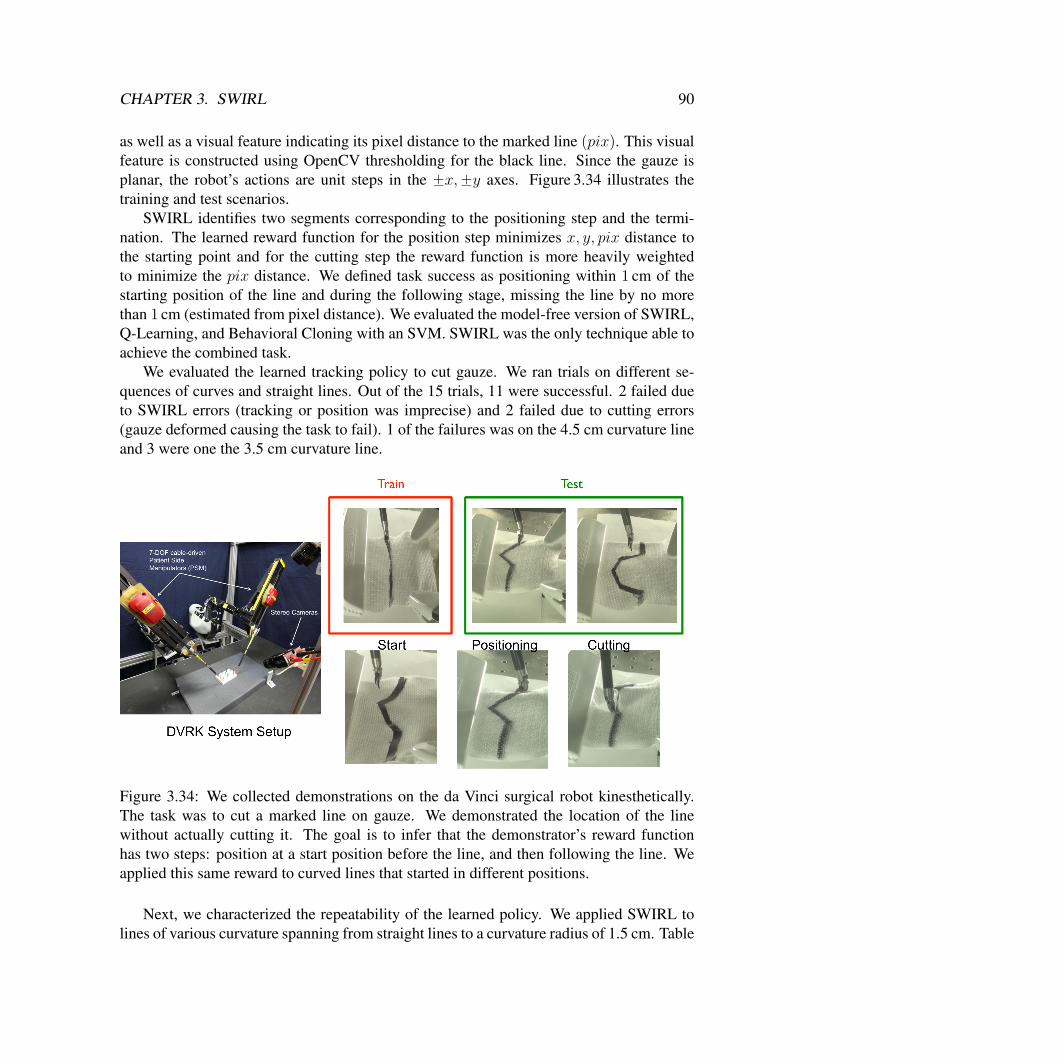
CHAPTER 3. SWIRL 90
as well as a visual feature indicating its pixel distance to the marked line ppixq. This visualfeature is constructed using OpenCV thresholding for the black line. Since the gauze isplanar, the robot’s actions are unit steps in the ˘x,˘y axes. Figure 3.34 illustrates thetraining and test scenarios.
SWIRL identifies two segments corresponding to the positioning step and the termi-nation. The learned reward function for the position step minimizes x, y, pix distance tothe starting point and for the cutting step the reward function is more heavily weightedto minimize the pix distance. We defined task success as positioning within 1 cm of thestarting position of the line and during the following stage, missing the line by no morethan 1 cm (estimated from pixel distance). We evaluated the model-free version of SWIRL,Q-Learning, and Behavioral Cloning with an SVM. SWIRL was the only technique able toachieve the combined task.
We evaluated the learned tracking policy to cut gauze. We ran trials on different se-quences of curves and straight lines. Out of the 15 trials, 11 were successful. 2 failed dueto SWIRL errors (tracking or position was imprecise) and 2 failed due to cutting errors(gauze deformed causing the task to fail). 1 of the failures was on the 4.5 cm curvature lineand 3 were one the 3.5 cm curvature line.
Figure 3.34: We collected demonstrations on the da Vinci surgical robot kinesthetically.The task was to cut a marked line on gauze. We demonstrated the location of the linewithout actually cutting it. The goal is to infer that the demonstrator’s reward functionhas two steps: position at a start position before the line, and then following the line. Weapplied this same reward to curved lines that started in different positions.
Next, we characterized the repeatability of the learned policy. We applied SWIRL tolines of various curvature spanning from straight lines to a curvature radius of 1.5 cm. Table

CHAPTER 3. SWIRL 91
Table 3.4: With 5 kinesthetic demonstrations of following marked straight lines on gauze,we applied SWIRL to learn to follow lines of various curvature. After 25 episodes of ex-ploration, we evaluated the policies on the ability to position in the correct cutting locationand track the line. We compare to SVM on each individual segment. SVM is comparablyaccurate on the straight line (training set) but does not generalize well to the curved lines.
Curvature Radius (cm) SVM Pos. Error (cm) SVM Tracking Error (cm) SWIRL Pos. Error (cm) SWIRL Tracking Error (cm)straight 0.46 0.23 0.42 0.21
4.0 0.43 0.59 0.45 0.333.5 0.51 1.21 0.56 0.383.0 0.86 3.03 0.66 0.572.5 1.43 - 0.74 0.872.0 - - 0.87 1.451.5 - - 1.12 2.44
3.4 summarizes the results on lines of various curvature. While the SVM approach did notwork on the combined task, we evaluated its accuracy on each individual step to illustratethe benefits of SWIRL. On following straight lines, SVM was comparable to SWIRL interms of accuracy. However, as the lines become increasingly curved, SWIRL generalizesmore robustly than the SVM. A single SVM has to learn both the positioning and cuttingpolicies. The combined policy is much more complicated than the individual policies, e.g.,go to a goal and follow a line.
Chapter 4
Alpha Clean: ReinforcementLearning For Data Cleaning
It is widely known that data cleaning is one of the most time-consuming steps of the dataanalysis process, and designing algorithms and systems to automate or partially automatedata cleaning continues to be an active area of research [24]. Automation in data cleaningis challenging because real-world data is highly variable. A single data set can have manydifferent types of data corruption such as statistical outliers, constraint violations, and du-plicates. Once an error is detected, there is a further question of how to repair this error,which often depends on how the data will be used in the future.
This variability creates a tension between generality and efficiency. While one mightwant a single cleaning framework that addresses all types of errors and repair operations, itis far more efficient to consider more specialized frameworks. Data cleaning tools are oftenhighly optimized for particular problems (e.g., see statistical outliers [46], enforcing logicalconstraints [24], entity resolution [64]). Consequently, a recent survey of industry suggeststhat data cleaning pipelines are often a patchwork of custom scripts and multiple special-ized systems [68]. The overhead to setup, learn, and manage multiple cleaning systemscan easily outweigh the benefits. Some data scientists eschew automated tools altogetherand simply write data cleaning programs from scratch. The customized programming ap-proach quickly becomes difficult to mantain and interpret; especially for users without dataengineering expertise [104].
A single cleaning system that exposes a sufficiently flexible interface is clearly desir-able; as long as the runtime and accuracy can be made comparable to existing alternatives.To achieve this, we turn to the contemporary AI literature, which has produced exciting re-sults such as AlphaGo [109] that were previously considered not possible. This work showsthat a combination of machine learning and massively parallelized search can effectivelyoptimize highly complex objective functions. Our main observation is that data cleaningis very similar to the search problems considered in AI [99]. The classic application is acomputer chess program that must plan a sequence of chess moves that change the state of
92
CHAPTER 4. ALPHA CLEAN 93
the board in order to maximize the likelihood of a checkmate. Likewise, in data cleaning,one is given a dirty relation and a way to measure data quality (e.g., number of integrityconstraints violated), and the data cleaning problem is to find a sequence of modificationsto the relation that maximize the data quality metric.
Most non-trivial problems are very hard without good search heuristics. Advances inmachine learning have made it possible to replace hand-crafted heuristics with automati-cally learned pruning functions that estimate the expected quality of candidate plans. Al-phaGo learned pruning heuristics using a neural network trained on data generated throughself-play [109]. This insight is highly relevant to data cleaning, where datasets tend tohave structure amenable to learning heuristics adaptively. Data errors are often systematicwhere they are correlated with with certain attributes and values in the dataset [69, 98].Consequently, as more data is cleaned, we can better identify common patterns to prioritizethe search on future data. We may not necessarily need a neural network for data clean-ing, but the overall algorithmic structure of AlphaGo, tree-search combined with a learnedheuristic, can be very useful.
AlphaClean is a new data cleaning system that is designed around a search-basedmodel. It takes as input a quality function that models the data quality of a relation asa real-value between r0, 1s and a language of parameterized data cleaning operators, andoutputs a sequence of data cleaning transformations (a cleaning program) from the lan-guage that seeks to maximize the quality function. This API imposes minimal restrictionson the quality function, giving it tremendous flexibility in terms of the data errors that itcan express. As a comparison, a recent system called Holoclean [98] is similar in thatit provides a rich interface to specify denial constraints and lookup tables, and integratesthem within a probabilistic model to more accurately resolve constraint violations. In con-trast, AlphaClean’s quality function is a user-defined function that can express arbitrarycombinations of denial constraints as well as statistical, quantitative, text formatting, andother classes of data errors. For instance, Section 4.4 shows how AlphaClean can performcleaning for machine learning applications by embedding machine learning training andevaluation within the quality function, while Section 4.4 combines entity resolution, outliercleaning, and functional dependency violations within the same function.
AlphaClean uses a best-first search that greedily appends data transformations to the setof best candidate programs seen so far, and adopts parallelization and pruning ideas fromthe search-based planning literature. In contrast to traditional search problems, where thesearch state (e.g., chess board) is compact and largely trivial to parallelize in a distributedsetting, the data cleaning search state is the size of the input dataset and introduces a trade-off between communication costs to share intermediate state and the degree of parallelismpossible. To further accelerate its runtime, AlphaClean can also encode problem-specificoptimizations as search pruning rules (e.g., disallowed transformation sequences) or mod-ifications to the data representation (e.g., clustering similar records). We find that manyoptimizations in existing cleaning systems may be cast as search pruning rules.
AlphaClean can adaptively learn pruning rules to avoid unprofitable search branchesduring the search process. While AlphaGo used a deep neural network and massive amounts
CHAPTER 4. ALPHA CLEAN 94
of training data to model the heurisitic, we found that a simple logistic regression classifierand training data gathered during the search process was sufficient to reduce the runtime bymultiple orders of magnitude. It is important to acknowledge that AlphaClean loses manyof the provable guarantees provided by specialized systems based on logical constraints,and is in some sense, best-effort. Across 8 real-world datasets used in prior data cleaningliterature, we show that AlphaClean matches or exceeds the cleaning accuracy and exhibitscompetitive run-times to state-of-the-art approaches that are specialized to a specific errordomain (constraint, statistical, or quantitative errors).
• Optimization: Existing cleaning pipelines must combine disparate cleaning solu-tions and manage glue code to transfer data between systems. However, data transfercan be a non-trivial portion of the total cleaning cost and recent work [93] has shownthat a common runtime can avoid data movement and improve runtimes by up to30ˆ.
• Generalization and Robustness: In contrast to existing cleaning systems, thatoutput a cleaning relation, AlphaClean outputs a composable cleaning program thatis both simpler to understand because it groups common fixes together, and can beapplied to new data. In addition, the cleaning program allows us to analyze cleaningsystems for overfitting. We indeed find that the complexity of the quality functionand cleaning language can lead to overfitting, and believe this is the case for any datacleaning system. We also show that simple changes to the quality function can act asregularization terms to control the degree of overfitting.
• Software Engineering: Users do not need to write and manage glue code; do notneed to manage ETL between systems; and do not need to learn system specificabstractions, languages, and assumptions. All of these are arguably intangible, butcritical friction points in the highly iterative cleaning process.
• New Cleaning Applications: We envision that a single API makes it possible tosupport an ecosystem of domain-specific cleaning specification libraries. For in-stance, interactive visualization interfaces akin to [1, 54, 133, 134] can directly trans-late user interactions into a wide range of cleaning constraints.
4.1 Problem SetupFirst, we overview the basic formalism of AlphaClean and present its relationship to relatedwork. We focus on data transformations that concern a single relational table. Let R be arelation over a set of attributes A,R denote the set of all possible relations over A, and r.abe the attribute value of a P A for row r P R. A data transformation T pRq : R ÞÑ R mapsan input relation instance R P R to a new (possibly cleaner) instance R1 P R that is unioncompatible with R. For instance, “replace all city attribute values equal to San Francisco
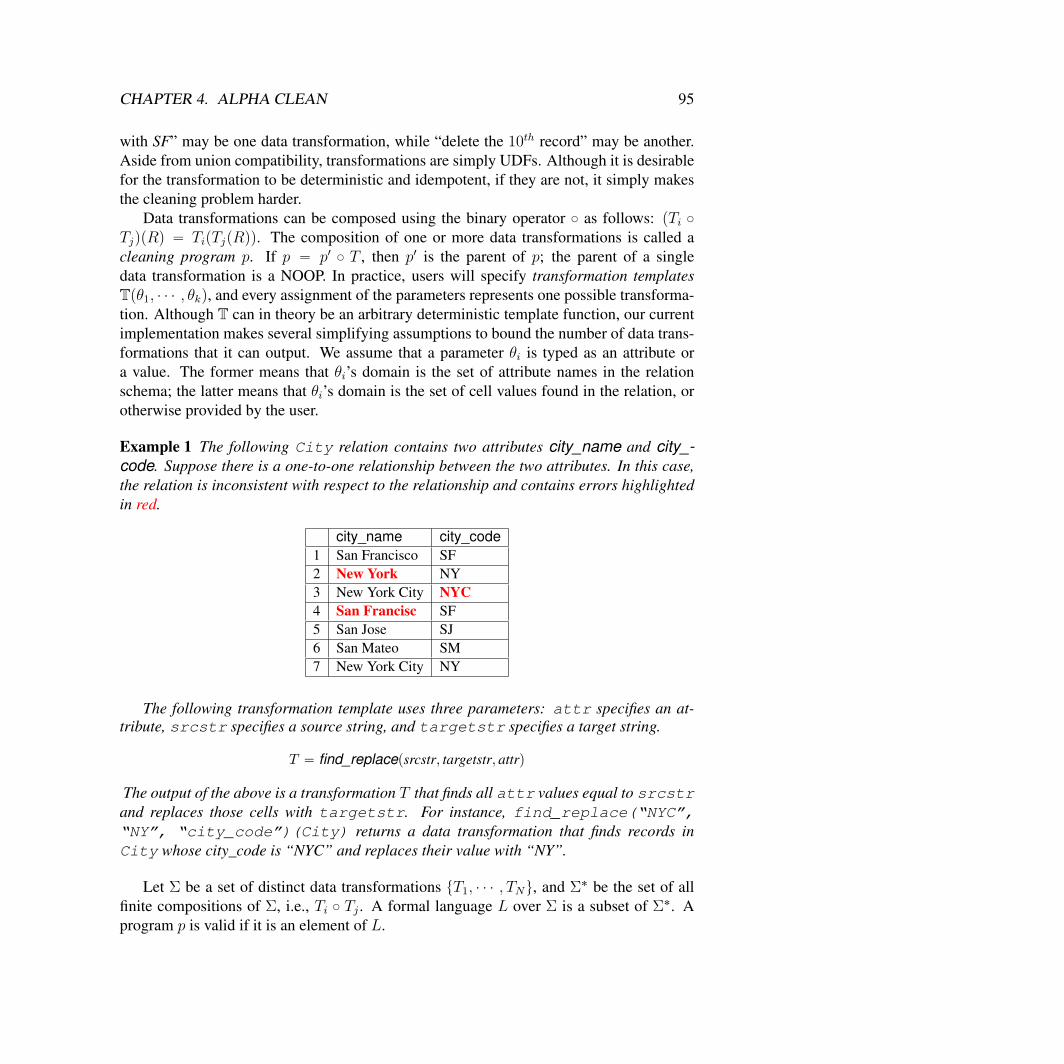
CHAPTER 4. ALPHA CLEAN 95
with SF” may be one data transformation, while “delete the 10th record” may be another.Aside from union compatibility, transformations are simply UDFs. Although it is desirablefor the transformation to be deterministic and idempotent, if they are not, it simply makesthe cleaning problem harder.
Data transformations can be composed using the binary operator ˝ as follows: pTi ˝TjqpRq “ TipTjpRqq. The composition of one or more data transformations is called acleaning program p. If p “ p1 ˝ T , then p1 is the parent of p; the parent of a singledata transformation is a NOOP. In practice, users will specify transformation templatesTpθ1, ¨ ¨ ¨ , θkq, and every assignment of the parameters represents one possible transforma-tion. Although T can in theory be an arbitrary deterministic template function, our currentimplementation makes several simplifying assumptions to bound the number of data trans-formations that it can output. We assume that a parameter θi is typed as an attribute ora value. The former means that θi’s domain is the set of attribute names in the relationschema; the latter means that θi’s domain is the set of cell values found in the relation, orotherwise provided by the user.
Example 1 The following City relation contains two attributes city_name and city_-code. Suppose there is a one-to-one relationship between the two attributes. In this case,the relation is inconsistent with respect to the relationship and contains errors highlightedin red.
city_name city_code1 San Francisco SF2 New York NY3 New York City NYC4 San Francisc SF5 San Jose SJ6 San Mateo SM7 New York City NY
The following transformation template uses three parameters: attr specifies an at-tribute, srcstr specifies a source string, and targetstr specifies a target string.
T “ find_replacepsrcstr, targetstr, attrq
The output of the above is a transformation T that finds all attr values equal to srcstrand replaces those cells with targetstr. For instance, find_replace(“NYC”,“NY”, “city_code”)(City) returns a data transformation that finds records inCity whose city_code is “NYC” and replaces their value with “NY”.
Let Σ be a set of distinct data transformations tT1, ¨ ¨ ¨ , TNu, and Σ˚ be the set of allfinite compositions of Σ, i.e., Ti ˝ Tj . A formal language L over Σ is a subset of Σ˚. Aprogram p is valid if it is an element of L.
CHAPTER 4. ALPHA CLEAN 96
Example 2 Continuing Example 1, Σ is defined as all possible parameterizations of find_-replace. Since many possible possible parameterizations are non-sensical (e.g., thesource string does not exist in the relation), we may bound Σ to only source and targetstrings present in each attribute’s instance domain (a standard assumption in other workas well [33]). In this case, there are 61 possible data transformations, and Σ˚ defines anyfinite composition of these 61 transformations. The language L can be further restricted tocompositions of up to k data transformations.
Finally, let QpRq : R ÞÑ r0, 1s be a quality function where 1 implies that the instance Ris clean, and a lower value correspond to a dirtier table. Since running a program p P L onthe initial dirty table Rdirty returns another table, QpppRdirtyqq returns a quality score foreach program in the language. Q is a UDF and we do not impose any restrictions on it. Infact, one experiment embeds training and evaluating a machine learning model within thequality function (Section 4.4). Another experiment shows that AlphaClean can be robustto random noise injected in the function (Section 4.4).
Even so, we call out two special cases that provide optimization opportunities. Wedefine two sub-classes of quality functions: row-separable and cell-separable quality func-tions. The former expresses the overall quality based on row-wise quality function qprq :R ÞÑ r0, 1s where 0 implies that the record is clean:
QpRq9ÿ
rPRqprq
Similarly, a cell-separable quality function means that there exists a cell-wise quality func-tion qpr, aq : pR ˆ Aq ÞÑ r0, 1s, such that the quality function is the sum of each cell’squality: QpRq9
ř
rPR
ř
aPA qpr, aq.These special cases are important because they can define hints on what types of trans-
formations are irrelevant. For example, if the quality function is cell-separable, and wehave identified that a set of cells C are dirty (e.g., they violate constraints), then we canignore transformations that do not modify cells in C. This restricts the size the languageand makes the problem much easier to solve.We are now ready to present data cleaning as the following optimization problem:
Problem 3 (cleanpQ,Rdirty, Lq) Given quality function Q, relation Rdirty, and languageL, find valid program p˚ P L that optimizes Q:
p˚ “ minpPL
QpppRdirtyqq.
p˚pRdirtyq returns the cleaned table, and p˚ can be applied to any table that is union compat-ible with Rdirty. A desirable property of this problem formulation is that it directly tradesoff runtime with cleaning accuracy and can be stopped at any time (though the cleaningprogram may be suboptimal). At the limit, AlphaClean simply explores L and identifiesthe optimal program.

CHAPTER 4. ALPHA CLEAN 97
Example 3 Continuing Example 1, let us assume the following functional dependenciesover the example relation: city_name Ñ city_code and city_code Ñ city_name. Wecan efficiently identify inconsistencies by finding the cities that map to ą 1 city code, andvice versa. Let such city names and codes be denotedDcity_name andDcity_code, respectively.QpRq is a cell-separable quality function where the cell-wise quality function is defined asqpr, aq “ 1´pr.a P Daq, such that r.a is 1 if the attribute value does not violate a functionaldependency, and 0 otherwise.
By searching through all possible programs up to length 3 in L, we can find a cleaningprogram based on find_replace that resolves all inconsistencies:
f i n d _ r e p l a c e ( New York , New York Ci t y , c i t y _ n a m e )f i n d _ r e p l a c e ( San Franc i s c , San Franc i sco , c i t y _ n a m e )f i n d _ r e p l a c e (NYC , NY , c i t y _ c o d e )
Approach Overview and ChallengesOur problem formulation is a direct instance of planning in AI [99], where an agent identi-fies a sequence of actions to achieve a goal. In our setting, the agent (AlphaClean) exploresa state space (R) from an initial state (the input relation) by following transitions (applyingTi P Σ) such that the sequence of actions is valid (within Σ˚) and the quality of the finalstate (QpRfinalq) is maximized.
For readers familiar with stochastic processes, this search problem is equivalent to adeterministic Markov Decision Process (MDP), where the states are R, the actions Σ, thetransition function updates the instance with the transformation, the initial state is the dirtyinstance Rdirty, and the reward function is Q.
One may be hesitant in adopting our problem formulation because, although it is suffi-ciently general to model many existing data cleaning problems, such generality often comesat the expense of runtime performance. The planning problem is APX-Hard, meaning theredoes not exist a polynomial time approximation unless P=NP. Let R be a single-attributerelation of Booleans. Let L be the set of all assignments to a single value. Given a list of NBoolean clauses over all the boolean variables, let Q assign to each record one minus thefraction of clauses that evaluate to true. This formulation is equivalent to MAX-SAT andsolution to the optimization problem.
For this reason, the key technical challenge is to show that AlphaClean can solve datacleaning problems with comparable run-time as existing specialized systems, and can beeasily extended to support new optimizations. Despite the problem’s worst-case complex-ity, recent successes in similar planning problems—ranging from AlphaGo [109] to auto-matically playing Atari video games [85] have shown that a prudent combination MachineLearning and distributed search can find practical solutions by leveraging the structure ofthe problem. Not every problem instance is as pathological as the worst case complexitysuggests, and there are many reasonable local optima.
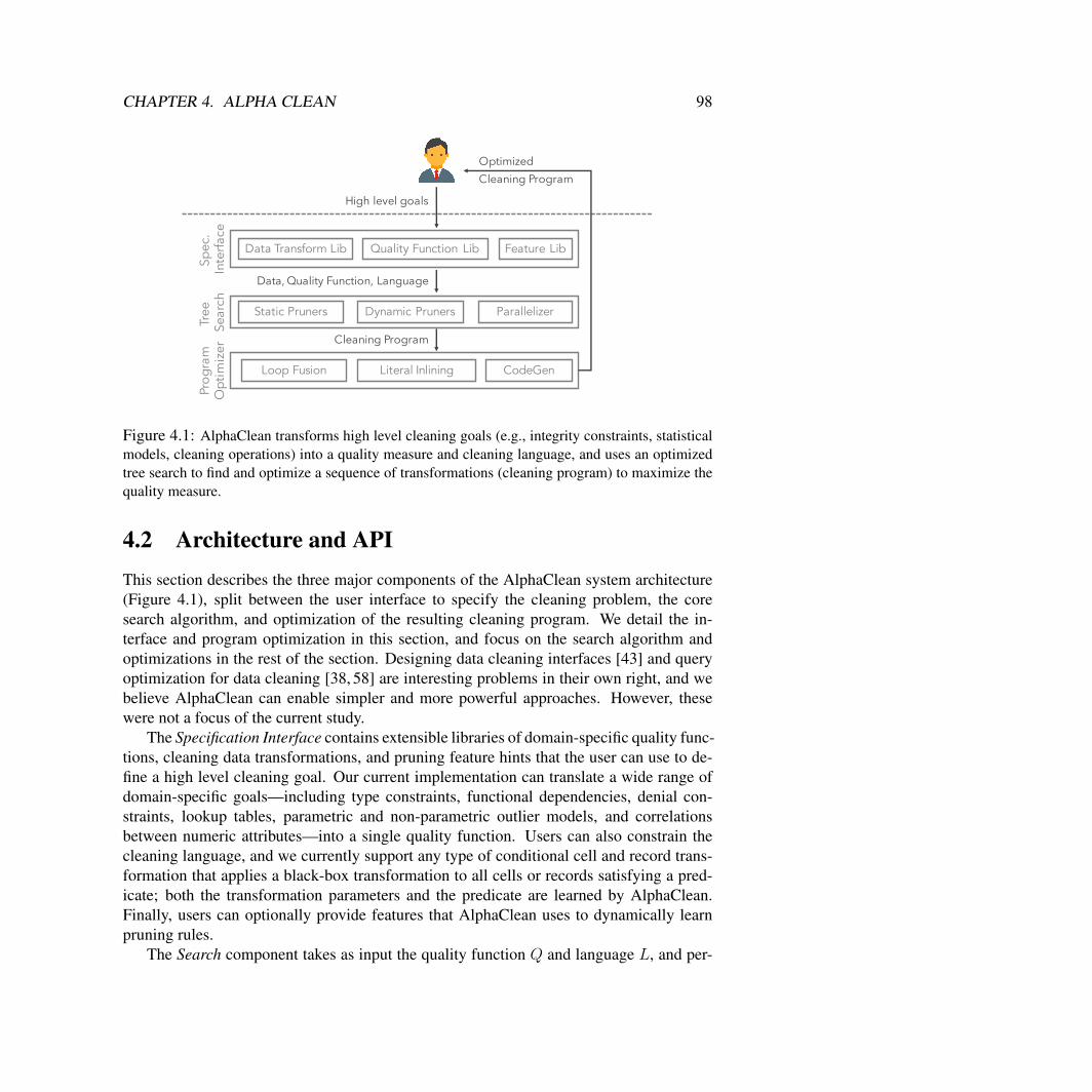
CHAPTER 4. ALPHA CLEAN 98
Data Transform Lib Quality Function Lib Feature Lib
Spec
. In
terfa
ceTr
ee
Sear
chPr
ogra
mO
ptim
izer
Static Pruners
Data, Quality Function, Language
High level goals
Dynamic Pruners Parallelizer
Loop Fusion Literal Inlining CodeGen
Cleaning Program
Optimized Cleaning Program
Figure 4.1: AlphaClean transforms high level cleaning goals (e.g., integrity constraints, statisticalmodels, cleaning operations) into a quality measure and cleaning language, and uses an optimizedtree search to find and optimize a sequence of transformations (cleaning program) to maximize thequality measure.
4.2 Architecture and APIThis section describes the three major components of the AlphaClean system architecture(Figure 4.1), split between the user interface to specify the cleaning problem, the coresearch algorithm, and optimization of the resulting cleaning program. We detail the in-terface and program optimization in this section, and focus on the search algorithm andoptimizations in the rest of the section. Designing data cleaning interfaces [43] and queryoptimization for data cleaning [38, 58] are interesting problems in their own right, and webelieve AlphaClean can enable simpler and more powerful approaches. However, thesewere not a focus of the current study.
The Specification Interface contains extensible libraries of domain-specific quality func-tions, cleaning data transformations, and pruning feature hints that the user can use to de-fine a high level cleaning goal. Our current implementation can translate a wide range ofdomain-specific goals—including type constraints, functional dependencies, denial con-straints, lookup tables, parametric and non-parametric outlier models, and correlationsbetween numeric attributes—into a single quality function. Users can also constrain thecleaning language, and we currently support any type of conditional cell and record trans-formation that applies a black-box transformation to all cells or records satisfying a pred-icate; both the transformation parameters and the predicate are learned by AlphaClean.Finally, users can optionally provide features that AlphaClean uses to dynamically learnpruning rules.
The Search component takes as input the quality function Q and language L, and per-
CHAPTER 4. ALPHA CLEAN 99
forms a greedy search heuristic to find a program p˚ P L that maximizes Q. Users cansupply hints that exploit the problem structure to reduce the runtime by pruning the searchspace and parallelizing the search. To bound the search space, users specify a maximumprogram length k. AlphaClean also supports three classes optimizations. Static pruninginvalidates candidate programs based on the program structure (sequence of actions). Forinstance, composing the same idempotent transformation (e.g., find_replace(SFO,SF, city_name)) in succession is unnecessary. Dynamic pruning can access the resultof a candidate program (search state) when making pruning decisions, and we propose anovel approach to learn automatic dynamic pruning rules that can reduce end-to-end run-times by up to 75% at the expense of slightly lower recall. Finally, AlphaClean parallelizesthe search in both shared memory and distributed settings. We describe the pruning rulesand parallelization optimization in detail in the following text.
Finally, once search component outputs the cleaning program p˚, the Program Opti-mizer performs query compilation optimizations and provides an API to add new opti-mizations. AlphaClean currently replaces variables with literal values whenever possible,inlines data transformations into loops that scan over the input relation, and uses loop fu-sion [25, 93] to avoid unnecessary scans over the input and intermediate relations for eachtransformation in p˚. Consider the program in Example 3. Since the find_replaceoperations do not conflict, it is inefficient to loop through over the relation instance threeseparate times. Since they do not conflict, it would be inefficient to execute them sequen-tially and iterate over the data three separate times. Instead, they can be fused:
f o r r i n rows :i f r [ c i t y_name ] == ‘New York ’ :
r [ c i t y_name ] = ‘New York Ci ty ’e l i f r [ c i t y_name ] == ‘ San F r a n c i s c ’ :
r [ c i t y_name ] = ‘ San F r a n c i s c o ’i f r [ c i t y _ c o d e ] == ‘NYC’
r [ c i t y _ c o d e ] = ‘NY’
These simple optimizations improve the final program runtime by up-to 20x, and weleave further improvements to future work (e.g., could be optimized with a framework likeWeld [93]).
4.3 Search AlgorithmWe now provide an overview of AlphaClean’s search algorithm and optimizations.
Naive Search ProceduresIn principle, any tree search algorithm over L would be correct. However, the traversalorder and expansion policy is important in this search problem. We describe the algorithmic

CHAPTER 4. ALPHA CLEAN 100
Figure 4.2: Main Algorithmic Loop
and practical reasons why two naive procedures—breadth-first search (BFS) and depth-firstsearch (DFS)—exhibit poor search runtimes.BFS: This approach extends each program in the search frontier with every possibledata transformation in Σ. To extend a candidate program lc with T P Σ, it evaluatesQppT ˝ lcqpRqq. Unfortunately, the frontier grows exponentially with each iteration. Ad-ditionally, evaluating every new candidate program T ˝ lc can be expensive if the inputrelation is large. Although the cost can be reduced by materializing lcpRq, it is not possibleto materialize all candidate programs in the frontier for all but the most trivial cleaningproblems. It is desirable to use asearch procedure that bounds the size of the frontier andthe materialization costs.
The first problem with this algorithm is that since each node in this tree o represents asequence of transformations. Evaluating the value of o can be very expensive since it wouldhave to evaluate the entire path to the root. o is a composition of many transformations andmay require a number of passes over the dataset. This can be avoided if we can materialize(either to disk or memory) the frontier,that is, for each node in the priority queue o P O, wehave a cached result of opRq. However, with BFS, the frontier is exponential in the supportof the language and the system would quickly run out of memory.DFS: Depth-first search only needs to materialize the intermediate results for a singleprogram at a time, however it is highly inefficient since the vast majority of programs thatit explores will have low quality scores.
CHAPTER 4. ALPHA CLEAN 101
Search Algorithm and OptimizationsBest-first search expands the most promising nodes chosen according to a specified costfunction. We consider a greedy version of this algorithm, which removes nodes on thefrontier that are more than γ times worse than the current best solution. Making γ smallermakes the algorithm asympotically consistent but uses more memory to store the frontier,whereas γ “ 1 is a pure greedy search with minimal memory requirements.
The frontier is modeled as a priority queue P where the priority is the quality of the can-didate program, and is initialized with a NOOP program with quality QpRq. The algorithmiteratively extends all programs in the queue with less than k transformations; a program pis extended by composing it with a transformation T in Σ. If the resulting program p1 is inthe language L, then we add it to the queue. Finally, let p be the highest quality programin the queue. The algorithm removes all programs whose quality is ă γ ˆ QpppRqq fromthe frontier. This process repeats until the candidate programs cannot be improved, or allprograms have k transformations.
In a naive and slow implementation, the above algorithm computes p’s quality by fullyrunning p on the input relation before running Q on the result, explores all possible datatransformation sequences, and runs sequentially. One of the benefits of its simple structureis that it is amenable to a rich set of optimizations to prune the search space, incrementallycompute quality functions, and parallelize the search. In fact, we find that many optimiza-tions in existing specialized cleaning systems can be cast in terms of the following classes.
We can materialize (either to disk or memory) the frontier,that is, for each node in thepriority queue p P P , we have a cached result of ppRq. Then, when we expand the nodesto p1 “ p ˝ t, we only have to incrementally evaluate tpRq. After the node is expanded,the result is added to the cache if it within γ of the best solution. The basic algorithmdescribed above is well-suited for this problem. Without the greediness, the frontier mightbe exponentially large leading to an impractical amount of materialization. By tuning γ,the user can essentially set how much memory is used for materialization.Static Pruning Rules are boolean functions that take a candidate program p as input anddecides whether it should be pruned. AlphaClean currently models static rules as regularexpressions over Σ. Static rules are can be viewed as filters over L.
static_ruleppq ÞÑ t0, 1u
For example, since the find-and-replace operations are idempotent, i.e., T pT pRqq “ T pRq,we may want to only consider the set of all sequences with no neighboring repeated trans-formations. Similarly, we may also want to prune all search branches that make no effect(i.e., find-and-replace New York with New York). These two regular expressions alone re-duce the above example’s language by 48% (from 226981 to 120050). Other rules, such asavoiding changes that undo previous changes T´1pT pRqq “ R, are similarly easy to add.Dynamic Pruning Rules also have access to the input relation and quality function, andcan make instance-specific pruning decisions.
dyn_rulepp,Q,Rq ÞÑ t0, 1u
CHAPTER 4. ALPHA CLEAN 102
For example, suppose Q is based on functional dependencies and is cell-separable, and wewant to ensure that cell-level transformations made by a candidate program p individuallyimproveQ. In this case, we find the cellsC that initially violate the functional dependenciesand ensure that the cells transformed by p are all in C. Applying this optimization, inaddition to the others in AlphaClean, to the example reduces the search space by 143ˆfrom 226,981 candidate programs to only 1582.
Since it can be challenging to hand-write pruning rules, there is a dynamic approach thatuses simple machine learning models to automatically identify the characteristics of candi-date programs to decide whether a particular search brach will be promising. In essence, itgenerates and refines static pruning rules during the search process.
For example, we may want to ensure that all the evaluations are “correlated” with thecost function–that is it makes modifications that are likely to affect the costs. This is pos-sible if the cost separable where we have a score for each cell. In this case, we can findall the cells in violation of the functional dependencies and make sure that the “source”field of the find-and-replace operations only match values that are in violation. These op-timizations are called “dynamic’ because they can be determined from the active domain(i.e., after applying a transformation, recalculate new optimization rules). Applying thisoptimization (in addition to the others) to the example reduces the search space to 1582evaluations v.s. 226981 unoptimized (143x reduction).Block-wise Cleaning: A major cost is that independent errors in the relation must becleaned sequentially in the search algorithm. For instance, records 2, 3, and 4 in the exam-ple exhibit independent errors and a fix for a given record does not affect the other records.Thus, if each record were cleaned in isolation, the search space would be Op|Σ|q. Unfor-tunately, the entire relation requires a program of three transformation to fix the records,which increases the search space to Op|Σ|3q.
The main insight in block-wise cleaning is that many errors are local to a small numberof records. In these cases, it is possible to partition R into a set of blocks B1, ¨ ¨ ¨ , Bm, ex-ecute the search algorithm over each block independently, and concatenate their programsto generate the final cleaning program. This gather-scatter approach can exponentially re-duce the search space for each block, and reduces the cost of evaluating super-linear qualityfunctions that require e.g., computing a pair-wise similarity scores for the input relation.For example, quality functions derived from functional dependencies can define blocks byexamining the violating tuples linked through the dependency. Similarly, users can definecustom partitioning functions or learn them via e.g., clustering algorithms. In our currentimplementation, we partition the input relation by cell or row if the quality function is cellor row separable.Parallel Program Evaluation: It is clear that the candidate programs can be evaluatedand pruning in a parallel fashion across multiple cores and multiple machines, and is oneof the major innovations in modern planning systems. However, unlike classic planningproblems where communications are small due to the compact size of each state, Alpha-Clean’s state size is determined by the relation instance, and can lead to prohibitively highcommunication costs and memory caching requirements. We describe how we manage the
CHAPTER 4. ALPHA CLEAN 103
trade-offs when parallelizing AlphaClean in shared memory and distributed settings.Materialization: Since each candidate program p1 “ p ˝ T is the composition of a pre-vious candidate program and a transformation, an obvious optimization is to materializethe output of ppRq and incrementally compute p1pRq as T pppRqq over the materialized in-termediate relation. Although this works well in a single threaded setting, memory andcommunication challenges arise when combining materialization with parallelization.
4.4 ExperimentsNext, we present experimental results that suggest three main conclusions: (1) as a singleframework, AlphaClean can achieve parity in terms of accuracy with state-of-the-art ap-proaches to a variety of different problems ranging from integrity constraint satisfaction,statistical data cleaning, and also data cleaning for machine learning, (2) it is possible tosignificantly reduce the runtime gap between AlphaClean and specialized frameworks us-ing simple pruning and distributed parallelization techniques, and (3) AlphaClean enablesautomatic data cleaning for datasets containing a mixture of error types in an acceptableamount of time.
Datasets and Cleaning TasksWe list the main characteristics of the 8 experimental datasets.Flight: The flight dataset [30] contains arrival time, departure time, and gate informationaggregated from 3 airline websites (AA, UA, Continental), 8 airport websites (e.g., SFO,DEN), and 27 third-party websites. There are 1200 flight departures and arrivals at airlinehubs recorded from each source. Each flight has a unique and globally consistent ID, andthe task is to reconcile data from different sources using the functional dependency IDÑarrival, departure, gate information.FEC: The election contributions dataset has 6,410,678 records, and 18 numerical, dis-crete, and text attributes. This dataset records the contribution amount and contributordemographic information e.g., name, address, and occupation. The task is to enforcecityÑzipcode, and match occupation to a codebook on canonical occupations. Thequality function is 1 if the occupation is in the codebook, and 0 otherwise; we penalize theedit distance between the original and edited occupation values.Malasakit: This dataset contains 1493 survey disaster preparedness responses from thePhilippines, with 15 numeric and discrete attributes. The task removes improper numericalvalues and remove dummy test records. This consists of domain integrity constraints thatforce the values to be within a certain dictionary.Physician: This dataset from Medicare.gov contains 37k US physican records, 10 at-tributes, with spelling errors in city names, zipcodes, and other text attributes. We use thedata cleaning rules described in [98], which consists of 9 functional dependencies.
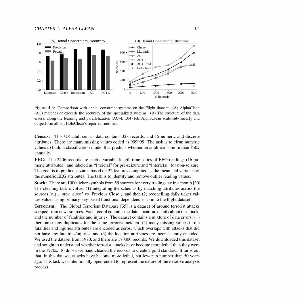
CHAPTER 4. ALPHA CLEAN 104
Figure 4.3: Comparison with denial constraint systems on the Flight dataset. (A) AlphaClean(AC) matches or exceeds the accuracy of the specialized systems. (B) The structure of the dataerrors, along the learning and parallelization (AC+L x64) lets AlphaClean scale sub-linearly andoutperform all but HoloClean’s reported runtimes.
Census: This US adult census data contains 32k records, and 15 numeric and discreteattributes. There are many missing values coded as 999999. The task is to clean numericvalues to build a classification model that predicts whether an adult earns more than $50kannually.EEG: The 2406 records are each a variable-length time-series of EEG readings (16 nu-meric attributes), and labeled as “Preictal” for pre-seizure and “Interictal” for non-seizure.The goal is to predict seizures based on 32 features computed as the mean and variance ofthe numeric EEG attributes. The task is to identify and remove outlier reading values.Stock: There are 1000 ticker symbols from 55 sources for every trading day in a month [30].The cleaning task involves (1) integrating the schemas by matching attributes across thesources (e.g., ‘prev. close’ vs ‘Previous Close’), and then (2) reconciling daily ticker val-ues values using primary-key-based functional dependencies akin to the flight dataset.Terrorism: The Global Terrorism Database [35] is a dataset of around terrorist attacksscraped from news sources. Each record contains the date, location, details about the attack,and the number of fatalities and injuries. The dataset contains a mixture of data errors: (1)there are many duplicates for the same terrorist incident, (2) many missing values in thefatalities and injuries attributes are encoded as zeros, which overlaps with attacks that didnot have any fatalities/injuries, and (3) the location attributes are inconsistently encoded.We used the dataset from 1970, and there are 170000 records. We downloaded this datasetand sought to understand whether terrorist attacks have become more lethal than they werein the 1970s. To do so, we hand cleaned the records to create a gold standard. It turns outthat, in this dataset, attacks have become more lethal, but fewer in number than 50 yearsago. This task was intentionally open-ended to represent the nature of the iterative analysisprocess.
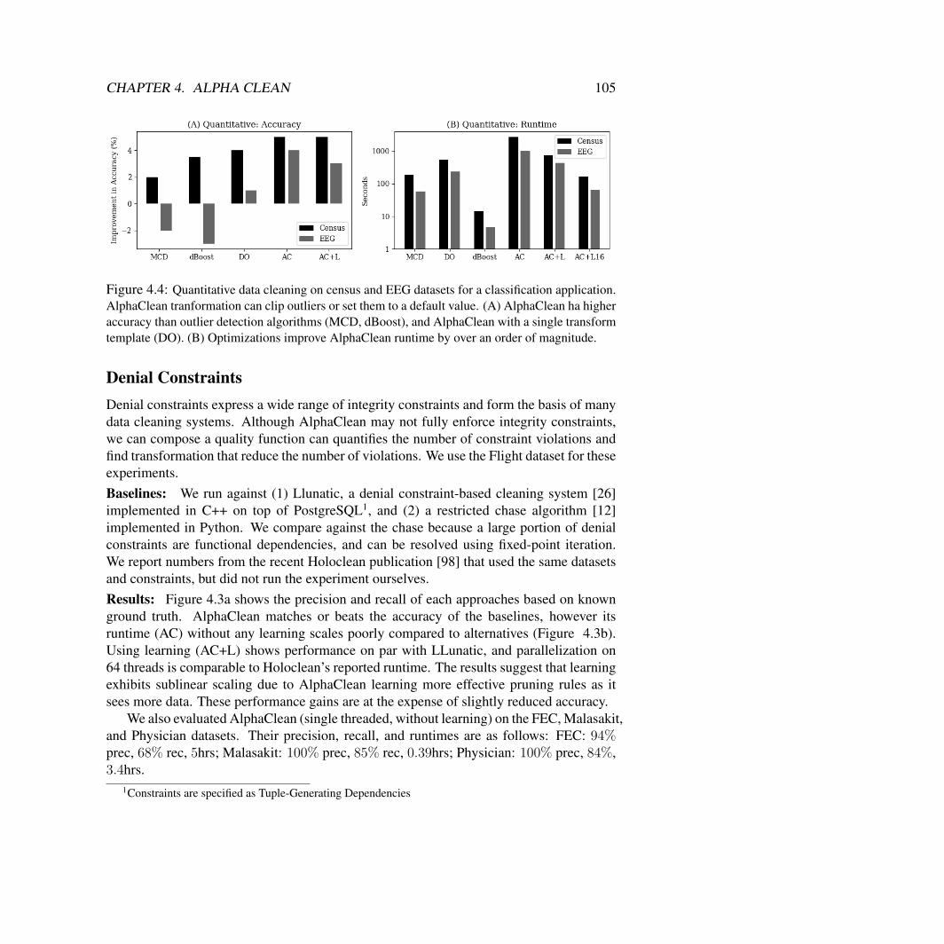
CHAPTER 4. ALPHA CLEAN 105
Figure 4.4: Quantitative data cleaning on census and EEG datasets for a classification application.AlphaClean tranformation can clip outliers or set them to a default value. (A) AlphaClean ha higheraccuracy than outlier detection algorithms (MCD, dBoost), and AlphaClean with a single transformtemplate (DO). (B) Optimizations improve AlphaClean runtime by over an order of magnitude.
Denial ConstraintsDenial constraints express a wide range of integrity constraints and form the basis of manydata cleaning systems. Although AlphaClean may not fully enforce integrity constraints,we can compose a quality function can quantifies the number of constraint violations andfind transformation that reduce the number of violations. We use the Flight dataset for theseexperiments.Baselines: We run against (1) Llunatic, a denial constraint-based cleaning system [26]implemented in C++ on top of PostgreSQL1, and (2) a restricted chase algorithm [12]implemented in Python. We compare against the chase because a large portion of denialconstraints are functional dependencies, and can be resolved using fixed-point iteration.We report numbers from the recent Holoclean publication [98] that used the same datasetsand constraints, but did not run the experiment ourselves.Results: Figure 4.3a shows the precision and recall of each approaches based on knownground truth. AlphaClean matches or beats the accuracy of the baselines, however itsruntime (AC) without any learning scales poorly compared to alternatives (Figure 4.3b).Using learning (AC+L) shows performance on par with LLunatic, and parallelization on64 threads is comparable to Holoclean’s reported runtime. The results suggest that learningexhibits sublinear scaling due to AlphaClean learning more effective pruning rules as itsees more data. These performance gains are at the expense of slightly reduced accuracy.
We also evaluated AlphaClean (single threaded, without learning) on the FEC, Malasakit,and Physician datasets. Their precision, recall, and runtimes are as follows: FEC: 94%prec, 68% rec, 5hrs; Malasakit: 100% prec, 85% rec, 0.39hrs; Physician: 100% prec, 84%,3.4hrs.
1Constraints are specified as Tuple-Generating Dependencies
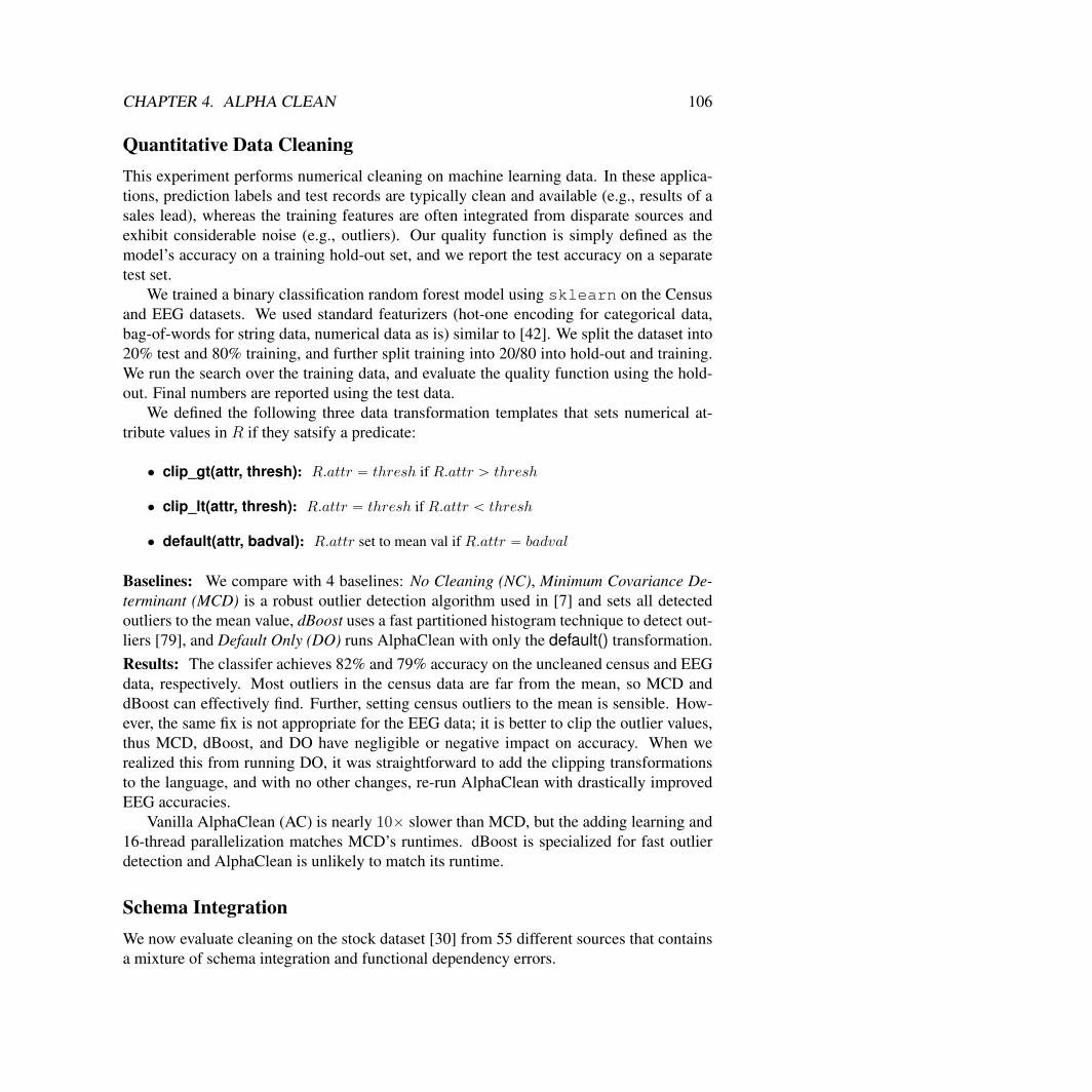
CHAPTER 4. ALPHA CLEAN 106
Quantitative Data CleaningThis experiment performs numerical cleaning on machine learning data. In these applica-tions, prediction labels and test records are typically clean and available (e.g., results of asales lead), whereas the training features are often integrated from disparate sources andexhibit considerable noise (e.g., outliers). Our quality function is simply defined as themodel’s accuracy on a training hold-out set, and we report the test accuracy on a separatetest set.
We trained a binary classification random forest model using sklearn on the Censusand EEG datasets. We used standard featurizers (hot-one encoding for categorical data,bag-of-words for string data, numerical data as is) similar to [42]. We split the dataset into20% test and 80% training, and further split training into 20/80 into hold-out and training.We run the search over the training data, and evaluate the quality function using the hold-out. Final numbers are reported using the test data.
We defined the following three data transformation templates that sets numerical at-tribute values in R if they satsify a predicate:
• clip_gt(attr, thresh): R.attr “ thresh if R.attr ą thresh
• clip_lt(attr, thresh): R.attr “ thresh if R.attr ă thresh
• default(attr, badval): R.attr set to mean val if R.attr “ badval
Baselines: We compare with 4 baselines: No Cleaning (NC), Minimum Covariance De-terminant (MCD) is a robust outlier detection algorithm used in [7] and sets all detectedoutliers to the mean value, dBoost uses a fast partitioned histogram technique to detect out-liers [79], and Default Only (DO) runs AlphaClean with only the default() transformation.Results: The classifer achieves 82% and 79% accuracy on the uncleaned census and EEGdata, respectively. Most outliers in the census data are far from the mean, so MCD anddBoost can effectively find. Further, setting census outliers to the mean is sensible. How-ever, the same fix is not appropriate for the EEG data; it is better to clip the outlier values,thus MCD, dBoost, and DO have negligible or negative impact on accuracy. When werealized this from running DO, it was straightforward to add the clipping transformationsto the language, and with no other changes, re-run AlphaClean with drastically improvedEEG accuracies.
Vanilla AlphaClean (AC) is nearly 10ˆ slower than MCD, but the adding learning and16-thread parallelization matches MCD’s runtimes. dBoost is specialized for fast outlierdetection and AlphaClean is unlikely to match its runtime.
Schema IntegrationWe now evaluate cleaning on the stock dataset [30] from 55 different sources that containsa mixture of schema integration and functional dependency errors.
CHAPTER 4. ALPHA CLEAN 107
Figure 4.5: Schema integration and functional dependency errors in the stock dataset. Cleaningschema integration (SI) or functional dependencies (DC) in isolation results in high precision butpoor recall. AlphaClean cleans both types of errors with higher recall, and is as fast as DC.
Baselines: We compare approaches for each error type in isolation. Schema Integration(SI) matches attributes based on attribute name string similarity, and Data Cleaning (DC)assumes schemas are consistent and enforces functions dependencies using a restrictedchase [12].
Results: The specialized cleaning approaches exhibit high precision but low recall, as theymiss records with multiple errors (Figure 4.5). AlphaClean can mix both tasks in the qualityfunction and has comparable precision with much higher recall. SI is significantly fastersince it only reads schema metadata, however AlphaClean with learning and 16 threads iscompetitive with DC.
Mixing Error ClassesThis experiment, we use the multi-error Terrorism dataset [35].Baselines: We hand-coded blocking-based entity matching (EM) and restricted chase(FD) algorithms in Python, and used dBoost for missing values. We also ran EM, dBoost,and Chase serially on the dataset (Combined).Results: Figure 4.7a shows that combining and cleaning all three classes of errors withinthe same AlphaClean framework (AC) achieves higher precision and recall than all base-lines. In fact, the combined baselines still does not achieve AlphaClean’s level of accuracybecause the cleaning operations need to be interleaved differently for different blocks. Al-though AlphaClean is slower than any individual baseline, parallelizing AlphaClean to 8threads is faster than the combined baseline by 2x.
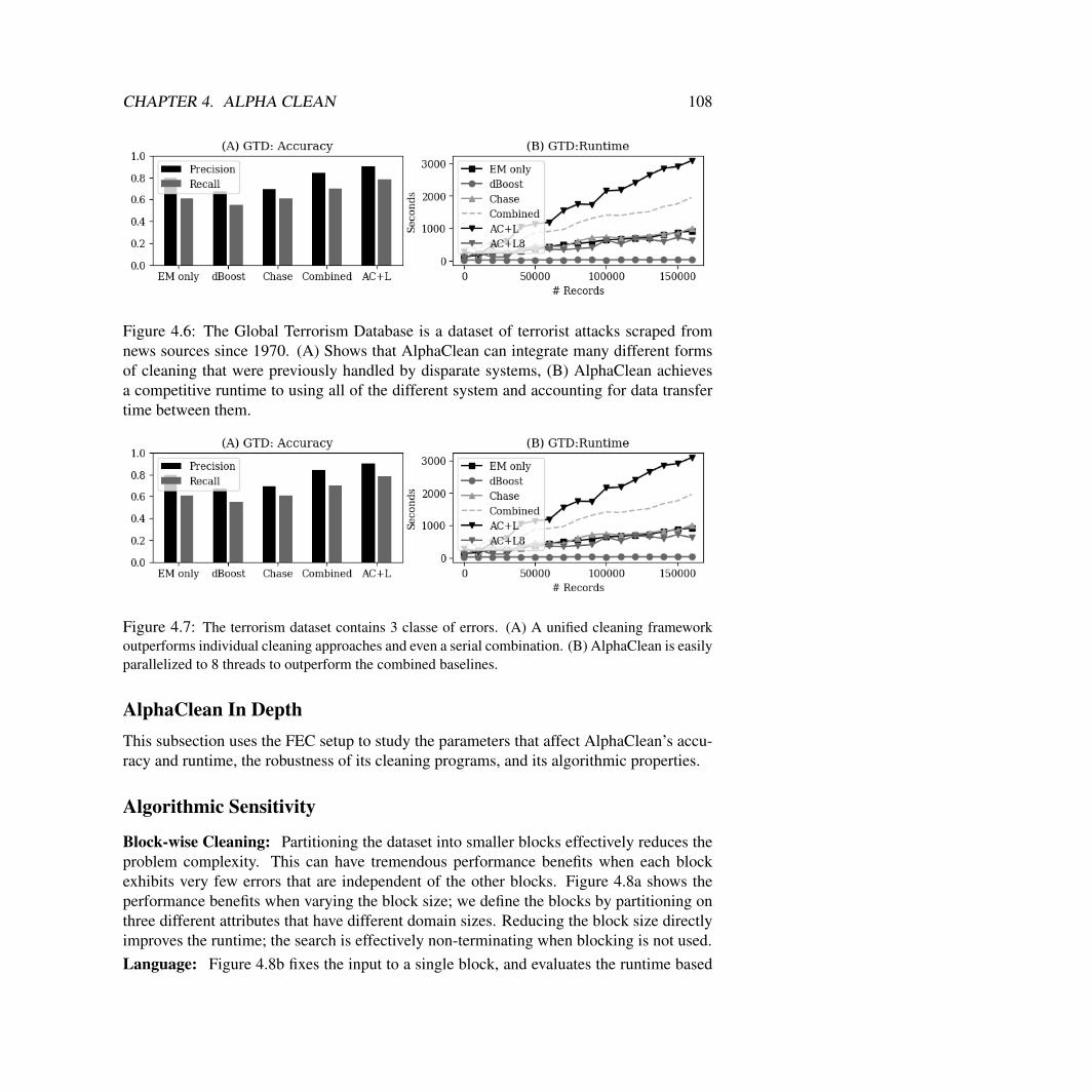
CHAPTER 4. ALPHA CLEAN 108
Figure 4.6: The Global Terrorism Database is a dataset of terrorist attacks scraped fromnews sources since 1970. (A) Shows that AlphaClean can integrate many different formsof cleaning that were previously handled by disparate systems, (B) AlphaClean achievesa competitive runtime to using all of the different system and accounting for data transfertime between them.
Figure 4.7: The terrorism dataset contains 3 classe of errors. (A) A unified cleaning frameworkoutperforms individual cleaning approaches and even a serial combination. (B) AlphaClean is easilyparallelized to 8 threads to outperform the combined baselines.
AlphaClean In DepthThis subsection uses the FEC setup to study the parameters that affect AlphaClean’s accu-racy and runtime, the robustness of its cleaning programs, and its algorithmic properties.
Algorithmic Sensitivity
Block-wise Cleaning: Partitioning the dataset into smaller blocks effectively reduces theproblem complexity. This can have tremendous performance benefits when each blockexhibits very few errors that are independent of the other blocks. Figure 4.8a shows theperformance benefits when varying the block size; we define the blocks by partitioning onthree different attributes that have different domain sizes. Reducing the block size directlyimproves the runtime; the search is effectively non-terminating when blocking is not used.Language: Figure 4.8b fixes the input to a single block, and evaluates the runtime based
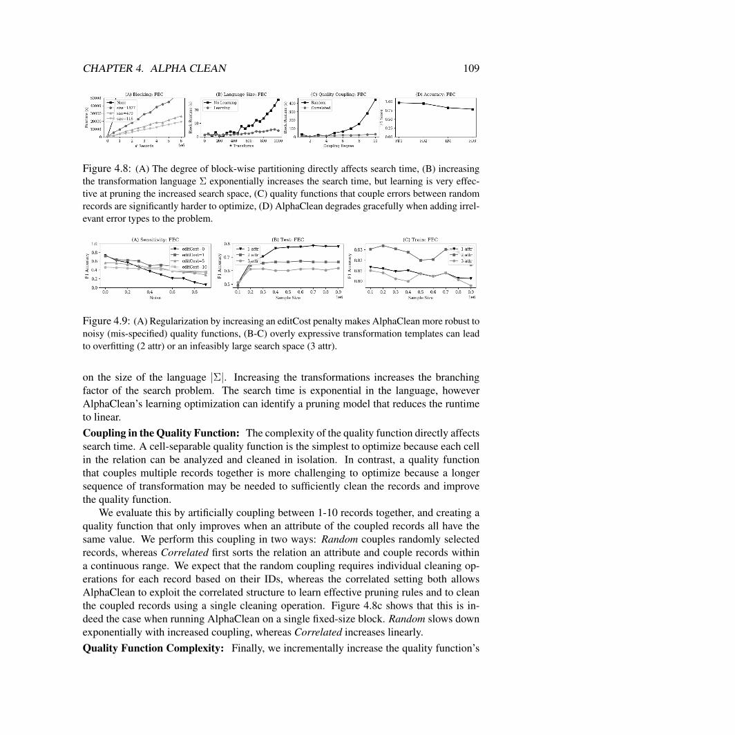
CHAPTER 4. ALPHA CLEAN 109
Figure 4.8: (A) The degree of block-wise partitioning directly affects search time, (B) increasingthe transformation language Σ exponentially increases the search time, but learning is very effec-tive at pruning the increased search space, (C) quality functions that couple errors between randomrecords are significantly harder to optimize, (D) AlphaClean degrades gracefully when adding irrel-evant error types to the problem.
Figure 4.9: (A) Regularization by increasing an editCost penalty makes AlphaClean more robust tonoisy (mis-specified) quality functions, (B-C) overly expressive transformation templates can leadto overfitting (2 attr) or an infeasibly large search space (3 attr).
on the size of the language |Σ|. Increasing the transformations increases the branchingfactor of the search problem. The search time is exponential in the language, howeverAlphaClean’s learning optimization can identify a pruning model that reduces the runtimeto linear.Coupling in the Quality Function: The complexity of the quality function directly affectssearch time. A cell-separable quality function is the simplest to optimize because each cellin the relation can be analyzed and cleaned in isolation. In contrast, a quality functionthat couples multiple records together is more challenging to optimize because a longersequence of transformation may be needed to sufficiently clean the records and improvethe quality function.
We evaluate this by artificially coupling between 1-10 records together, and creating aquality function that only improves when an attribute of the coupled records all have thesame value. We perform this coupling in two ways: Random couples randomly selectedrecords, whereas Correlated first sorts the relation an attribute and couple records withina continuous range. We expect that the random coupling requires individual cleaning op-erations for each record based on their IDs, whereas the correlated setting both allowsAlphaClean to exploit the correlated structure to learn effective pruning rules and to cleanthe coupled records using a single cleaning operation. Figure 4.8c shows that this is in-deed the case when running AlphaClean on a single fixed-size block. Random slows downexponentially with increased coupling, whereas Correlated increases linearly.Quality Function Complexity: Finally, we incrementally increase the quality function’s
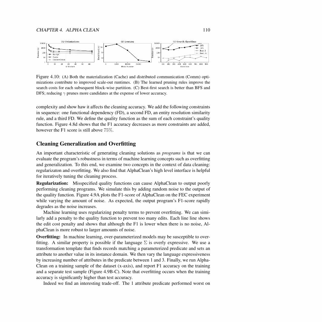
CHAPTER 4. ALPHA CLEAN 110
Figure 4.10: (A) Both the materialization (Cache) and distributed communication (Comm) opti-mizations contribute to improved scale-out runtimes. (B) The learned pruning rules improve thesearch costs for each subsequent block-wise partition. (C) Best-first search is better than BFS andDFS; reducing γ prunes more candidates at the expense of lower accuracy.
complexity and show haw it affects the cleaning accuracy. We add the following constraintsin sequence: one functional dependency (FD), a second FD, an entity resolution similarityrule, and a third FD. We define the quality function as the sum of each constraint’s qualityfunction. Figure 4.8d shows that the F1 accuracy decreases as more constraints are added,however the F1 score is still above 75%.
Cleaning Generalization and OverfittingAn important characteristic of generating cleaning solutions as programs is that we canevaluate the program’s robustness in terms of machine learning concepts such as overfittingand generalization. To this end, we examine two concepts in the context of data cleaning:regularizaton and overfitting. We also find that AlphaClean’s high level interface is helpfulfor iteratively tuning the cleaning process.Regularization: Misspecified quality functions can cause AlphaClean to output poorlyperforming cleaning programs. We simulate this by adding random noise to the output ofthe quality function. Figure 4.9A plots the F1-score of AlphaClean on the FEC experimentwhile varying the amount of noise. As expected, the output program’s F1-score rapidlydegrades as the noise increases.
Machine learning uses regularizing penalty terms to prevent overfitting. We can simi-larly add a penalty to the quality function to prevent too many edits. Each line line showsthe edit cost penalty and shows that although the F1 is lower when there is no noise, Al-phaClean is more robust to larger amounts of noise.Overfitting: In machine learning, over-parameterized models may be susceptible to over-fitting. A similar property is possible if the language Σ is overly expressive. We use atransformation template that finds records matching a parameterized predicate and sets anattribute to another value in its instance domain. We then vary the language expressivenessby increasing number of attributes in the predicate between 1 and 3. Finally, we run Alpha-Clean on a training sample of the dataset (x-axis), and report F1 accuracy on the trainingand a separate test sample (Figure 4.9B-C). Note that overfitting occurs when the trainingaccuracy is significantly higher than test accuracy.
Indeed we find an interesting trade-off. The 1 attribute predicate performed worst on
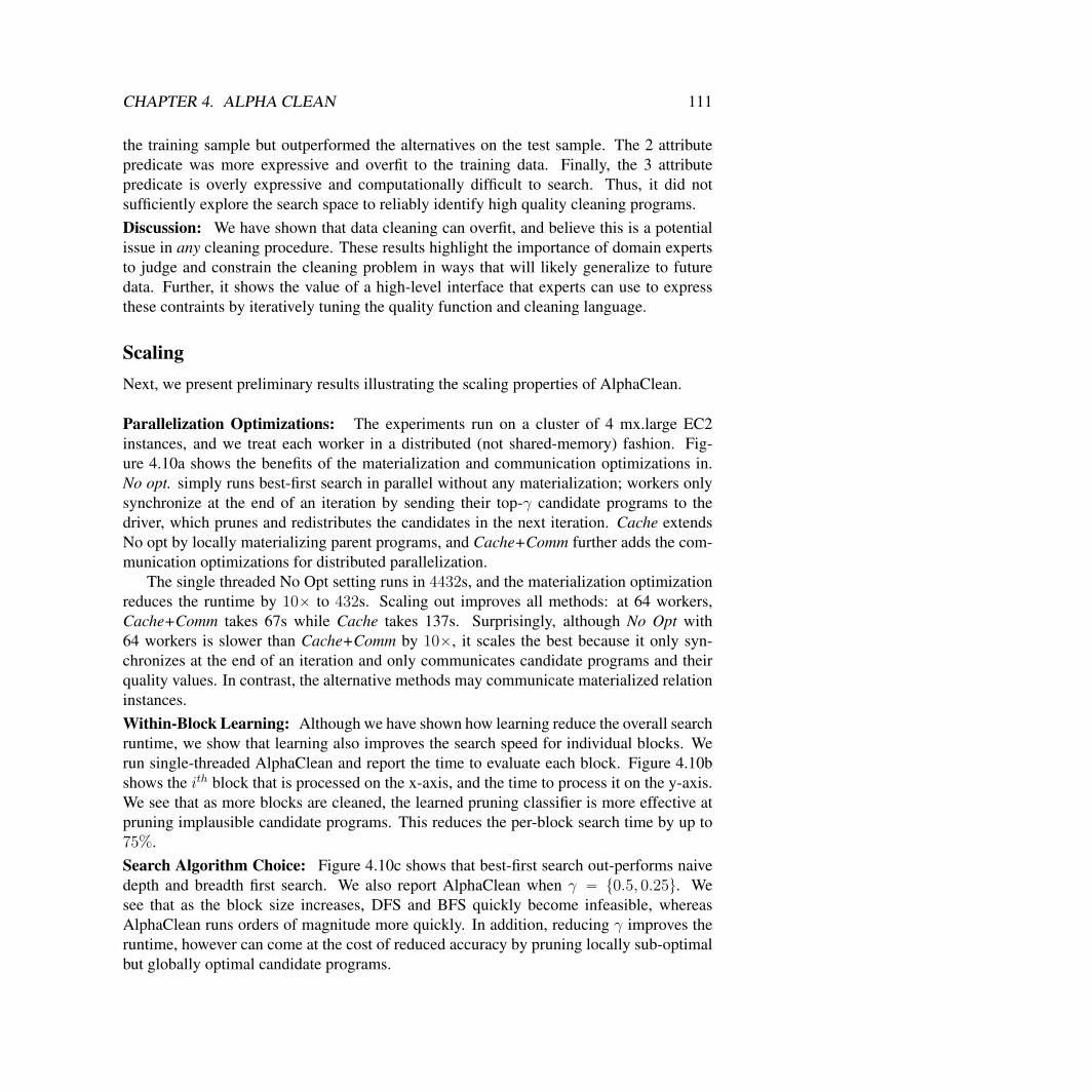
CHAPTER 4. ALPHA CLEAN 111
the training sample but outperformed the alternatives on the test sample. The 2 attributepredicate was more expressive and overfit to the training data. Finally, the 3 attributepredicate is overly expressive and computationally difficult to search. Thus, it did notsufficiently explore the search space to reliably identify high quality cleaning programs.Discussion: We have shown that data cleaning can overfit, and believe this is a potentialissue in any cleaning procedure. These results highlight the importance of domain expertsto judge and constrain the cleaning problem in ways that will likely generalize to futuredata. Further, it shows the value of a high-level interface that experts can use to expressthese contraints by iteratively tuning the quality function and cleaning language.
ScalingNext, we present preliminary results illustrating the scaling properties of AlphaClean.
Parallelization Optimizations: The experiments run on a cluster of 4 mx.large EC2instances, and we treat each worker in a distributed (not shared-memory) fashion. Fig-ure 4.10a shows the benefits of the materialization and communication optimizations in.No opt. simply runs best-first search in parallel without any materialization; workers onlysynchronize at the end of an iteration by sending their top-γ candidate programs to thedriver, which prunes and redistributes the candidates in the next iteration. Cache extendsNo opt by locally materializing parent programs, and Cache+Comm further adds the com-munication optimizations for distributed parallelization.
The single threaded No Opt setting runs in 4432s, and the materialization optimizationreduces the runtime by 10ˆ to 432s. Scaling out improves all methods: at 64 workers,Cache+Comm takes 67s while Cache takes 137s. Surprisingly, although No Opt with64 workers is slower than Cache+Comm by 10ˆ, it scales the best because it only syn-chronizes at the end of an iteration and only communicates candidate programs and theirquality values. In contrast, the alternative methods may communicate materialized relationinstances.Within-Block Learning: Although we have shown how learning reduce the overall searchruntime, we show that learning also improves the search speed for individual blocks. Werun single-threaded AlphaClean and report the time to evaluate each block. Figure 4.10bshows the ith block that is processed on the x-axis, and the time to process it on the y-axis.We see that as more blocks are cleaned, the learned pruning classifier is more effective atpruning implausible candidate programs. This reduces the per-block search time by up to75%.Search Algorithm Choice: Figure 4.10c shows that best-first search out-performs naivedepth and breadth first search. We also report AlphaClean when γ “ t0.5, 0.25u. Wesee that as the block size increases, DFS and BFS quickly become infeasible, whereasAlphaClean runs orders of magnitude more quickly. In addition, reducing γ improves theruntime, however can come at the cost of reduced accuracy by pruning locally sub-optimalbut globally optimal candidate programs.

CHAPTER 4. ALPHA CLEAN 112
Program StructureFinally, we present results describing the structure of the data cleaning programs foundwith AlphaClean. It is often the case that the program found by AlphaClean is a concisedescription of the needed data cleaning operations, that is, the total number of cell edits ismuch larger than the length of the program. We consider the FEC dataset, the EEG dataset,and GTD dataset.
Sometimes, the program (FEC and GTD) encodes a significant amount of literal values.This happens in entity matching type problems. For these problems, the program length isrelatively large, however, the number of cells modified is even larger (up to 10x more). Fordatasets like the EEG dataset, the program is very concise (26x smaller than the numberof cells modified). Numerical thresholds are generalize better than categorical find-and-replace operations.
Program Length Cells ModifiedFEC 6416 78342EEG 6 161GTD 1014 104992
Chapter 5
Reinforcement Learning For SQLQuery Optimization
Joins are a ubiquitous primitive in data analytics. The rise of new tools, such as Tableau,that automatically generate queries has led to renewed interest in efficiently executing SQLqueries with several hundred joined relations. Since most relational database managementsystems support only dyadic join operators (joining two tables) as primitive operations, aquery optimizer must choose the “best” sequence of two-way joins to achieve the k-wayjoin of tables requested by a query.
5.1 Problem SetupThe problem of optimally nesting joins is, of course, combinatorial and is known to beNP-Hard. To make matters worse, the problem is also known to be practically challengingsince a poor solution can execute several orders of magnitude slower than an optimal one.Thus, many database systems favor “exact” solutions when the number of relations aresmall but switch to approximations after a certain point. For example, PostgreSQL usesdynamic programming when the query has less than 12 relations and then switches to agenetic algorithm for larger queries. Similarly, IBM DB2 uses dynamic programming andswitches to a greedy strategy when the number of relations grows.
Traditionally, exact optimization is addressed with a form of sequential dynamic pro-gramming. The optimizer incrementally builds optimal joins on subsets of relations andmemoizes the optimal join strategy as well as the cost-to-go based on an internal costmodel. This dynamic programming algorithm still enumerates all possible join sequencesbut shares computation where possible. Natually, this enumeration process is sensitivewhen the underlying cost models in the RDBMS are inaccurate. Care has to be taken toavoid enumerating plans that are risky, or high variance, if table sizes or system parametersare not known exactly. Some work has considered incorporating feedback to the cost modelafter execution to improve the model for future optimization instances.
113
CHAPTER 5. QUERY OPTIMIZATION 114
As it stands there are three challenges that modern join optimizers try to simultaneouslyaddress: (1) pruning a large space of possible plans, (2) hedging against uncertainty, and(3) feedback from query evaluation. For each of these three problems, the communityhas proposed numerous algorithms, approximations, and heuristics to address them. Oftenthe dominant techniques are sensitive to both the particular workload and the data. Theengineering complexity of implementing robust solutions to all of these challenges canbe very significant, and commerical solutions are often incomplete—where some level ofquery engineering (by creating views and hints) from the developer is needed.
Recent advances in Artificial Intelligence may provide an unexpected perspective onthis impasse. The emergence of deep reinforcement learning, e.g., AlphaGo, has presenteda pragmatic solution to many hard Markov Decision Processes (MDPs). In an MDP, thereis a decision making agent who makes a sequence of decisions to effect change on a sys-tem that processes these decisions and updates the system’s internal state (potentially non-deterministically). MDPs are Markovian in the sense that the system’s current state and theagent’s decision completely determines any future evolution. The solution to an MDP is adecision to make at every possible state. We show that the join optimization can be posedas an MDP where the state is the join graph and decisions are edge contractions on thisgraph.
Given this formulation, the Deep Q Network (DQN) algorithm can be applied, andin essence, this formulation gives us an approximate dynamic programming algorithm.Instead of exactly memoizing subplans in a table with cost-to-go estimates as in dynamicprogramming, DQN represents this table with a neural network of a fixed size. This allowsthe algorithm to “estimate” the cost-to-go of subplans even if they have not been previouslyenumerated.
This learning based approach gives us flexibility in designing new intelligent enumera-tion strategies by manipulating how the neural network is trained and how it represents thesubplans. For example, the neural network allows us to efficiently share query processinginformation across planning instances with the neural network parameters and learn frompreviously executed queries. The consequence is enumeration strategies tuned to the spe-cific workload and data. We can also vary the features used to represent the subplans, toallow the network to capture different properties like interesting orders and physical op-erator selection. We can also train the neural network with observations of actual queryexecution times and make through repeated executions make it robust to uncertainty.
In short, Deep RL provides a new algorithmic framework for thinking about join enu-meration. We can architect an entire query processing stack around this Deep RL frame-work. We explore this architecture and evaluate in what situations its behavior is moredesirable (either in terms of cost or planning time) compared to classical approaches. Oursystem is built on Apache Calcite and integrates with Apache Spark, Postgres SQL, and aninternal join planning simulator. We present results on a variety of experimental workloadsand datasets.
CHAPTER 5. QUERY OPTIMIZATION 115
5.2 BackgroundFirst, we will introduce the algorithmic connection between Reinforcement Learning andthe join optimization problem.
Query ModelConsider the following query model. Let tR1, ..., RT u define a set of relations, and letR “ R1ˆ ...ˆRT denote the cartesian product. We define an inner join query q as a subsetof q Ď R as defined by a conjunctive predicate ρ1^...^ρj where each expression ρ is binaryboolean function of the attributes of two relations in the set ρ “ Ri.at“, ! “,ą,ăuRj.bq.We assume that the number of conjunctive expressions is capped at some fixed sizeN . Wefurther assume that the join operation is commutative, left associative, and right associative.Extending our work to consider left and right outer joins is very straight-forward but wewill defer that to that to future work.
We will use the following database of three relations denoting employee salries as arunning example throughout the chapter:
Emppid, name, rankq
Posprank, title, codeq
Salpcode, amountq
Consider the following join query:
SELECT ∗FROM Emp , Pos , S a lWHERE Emp . r ank = Pos . r ank ANDPos . code = S a l . code
In this schema, R denotes the set of tuples tpe P Emp, p P Pos, s P Salqu. There are twopredicates ρ1 “ Emp.rank “ Pos.rank and ρ2 “ Pos.code “ Sal.code, combined witha conjunction. One has several possible options on how to execute that query. For example,one could execute the query as Emp ’ pSal ’ Posq. Or, one could execute the query asSal ’ pEmp ’ Posq.
Graph Model of EnumerationEnumerating the set of all possible dyadic join plans can be expressed as operations on agraph representing the join relationships requested by a query.
Definition 5 (Query Graph) Let G define an undirected graph called the query graph,where each relation R is a vertex and each ρ defines an edge between vertices. The numberof connected components of G are denoted by κG.
CHAPTER 5. QUERY OPTIMIZATION 116
Each possible dyadic join is equivalent to a combinatorial operation called a graphcontraction.
Definition 6 (Contraction) Let G “ pV,Eq be a query graph with V defining the set ofrelations and E defining the edges from the join predicates. A contraction c is a functionof the graph parametrized by a tuple of vertices c “ pvi, vjq. Applying c to the graph Gdefines a new graph with the following properties: (1) vi and vj are removed from V , (2) anew vertex vij is added to V , and (3) the edges of vij are the union of the edges incident tovi and vj .
Each contraction reduces the number of vertices by 1. And, that every feasible dyadicjoin plan can be described as a sequence of such contractions c1 ˝ c2... ˝ cT until |V | “ κG.Going back to our running example, suppose we start with a query graph consisting ofthe vertices pEmp, Pos, Salq. Let the first contraction be c1 “ pEmp, Posq, this leadsto a query graph where the new vertices are pEmp ` Pos, Salq. Applying the only re-maining possible contraction, we arrive at a single remaining vertex Sal ` pEmp ` Posqcorresponding to the join plan Sal ’ pEmp ’ Posq.
The join optimization is to find the best possible one of these contraction sequences.Assume that we have access to a cost model J , which is a function that can estimate theincremental cost of a particular contraction Jpcq ÞÑ R`.
Problem 4 (Join Optimization Problem) Let G define a query graph and J define a costmodel. Find a sequence of c1 ˝ c2... ˝ cT terminating in |V | “ κG to minimize:
minc1,...,cT
Tÿ
i“1
Jpciq
Note how the “Principle of Optimality” arises in Problem 4. Applying each contractiongenerates a subproblem of a smaller size (a query graph with one less vertex). Each ofthese subproblems must be solved optimally in any optimal solution. Also note that thismodel can capture physical operator selection as well. The set of allowed contractions canbe typed with an eligible join type e.g., c “ pvi, vj, hashq or c “ pvi, vj, indexq.
Greedy vs. OptimalA greedy solution to this problem is to optimize each ci independently. The algorithmproceeds as follows: (1) start with the query graph, (2) find the lowest cost contraction,(3) update the query graph and repeat until only one vertex is left. The greedy algorithm,of course, does not consider how local decision might affect future costs. Consider ourrunning example query with the following costs (assume symmetry):
JpEP q “ 100, JpSP q “ 90, JppEP qSq “ 10, JppSP qEq “ 50
CHAPTER 5. QUERY OPTIMIZATION 117
The greedy solution would result in a cost of 140 (because it neglects the future effectsof a decision), while the optimal solution has a cost of 110. However, there is an up-side, this greedy algorithm has a computational complexity of Op|V |3q—despite the super-exponential search space.
The decision at each index needs to consider the long-term value of its actions whereone might have to sacrifice a short term benefit for a long term payoff. Consider the follow-ing way of expressing the optimization problem in the problem statement for a particularquery graph G:
V pGq “ minc1,...,cT
Tÿ
i“1
Jpciq (3)
We can concisely describe Equation 3 as the function V pGq, i.e., given the initial graphG, what is the value of acting optimally till the end of the decision horizon. This functionis conveniently named the value function. Bellman’s “Principle of Optimality” noted thatoptimal behavior over an entire decision horizon implies optimal behavior from any startingindex t ą 1 as well, which is the basis for the idea of dynamic programming. So, V pGq canbe then defined recursively for any subsequent graph G1 generated by future contractions:
V pGq “ minct Jpcq ` γ ¨ V pG1q u (4)
Usually, write this value recursion in the following form:
QpG, cq “ Jpcq ` γ ¨ V pG1q
Leading to the following recursive definition of the Q-Function (or cost-to-go function):
QpG, cq “ Jpcq ` γ ¨minc1QpG1, c1q (5)
The Q-Function describes the long-term value of each contraction. That means at eachG1 local optimization of minc1 QpG
1, c1q is sufficient to derive an optimal sequence of de-cisions. Put another way, the Q-function is a hypothetical cost function on which greedydescent is optimal and equivalent to solving the original problem. If we revisit the greedyalgorithm, and revise it as follows: (1) start with the query graph, (2) find the lowest Q-value contraction, (3) update the query graph and repeat. This algorithm has a computa-tional complexity of Op|V |3q (just like the greedy algorithm) but is provably optimal.
The Q-function is implicitly stored as a table in classical dynamic programming ap-proaches, such as the System R enumeration algorithm. In the System R algorithm, thereis a hash table that maps sets of joined relations to their lowest-cost access path:
HashMap<Set < R e l a t i o n > , ( Plan , Long ) > b e s t J o i n s ;
As the algorithm enumerates more subplans, if a particular relation set exists in the tableit replaces the access path if the enumerated plan has a lower cost than one in the table.We could equivalently write a different hash table that moves around the elements on thetable described above. Instead of a set of relations mapping to a plan and a cost, we couldconsider a set of relations and a plan mapping to a cost:
CHAPTER 5. QUERY OPTIMIZATION 118
HashMap <( Set < R e l a t i o n > , P l an ) , Long> b e s t Q J o i n s ;
Learning the Q-FunctionThis change would be less efficient implementation in classical dynamic programming, butit crucially allows us to setup a machine learning problem. What if we could regress fromfeatures of (Set<Relation>, Plan) to a cost based on a small number of observa-tions? Instead of a Q-Function as a table, it is parametrized as a model:
QθpfG, fcq « QpG, cq
where fG is a feature vector representing the query graph and fc is a feature vector rep-resenting the particular contraction on the graph. θ defines the neural network parametersthat represent this function.
The basic strategy to generate observational data, that is, real executions of join plans,and optimize θ to best explain the observations. Such an optimization problem is a keymotivation of a general class of algorithms called Reinforcement Learning [121], wherestatistical machine learning techniques are used to approximate optimal behavior whileobserving substantially less data that full enumeration.
For those familiar with the AI literature, this problem defines a Markov Decision Pro-cess. G is exactly a representation of the state and c is a representation of the action. Theutility function (or reward) of this process is the negative overall runtime. The objectiveof the planning problem is to find a policy, which is a map from a query graph to the bestpossible join c.
In the popular Q-Learning approach [121], the algorithm enumerates random samplesof decision sequences containing pG, c, runtime,G1q tuples forming a trajectory. Fromthese tuples, one can calculate the following value:
yi “ runtime` arg maxu
QθpG1, cq
Each of the yi can be used to define a loss function since if Q were the true Q function,then the following recurrence would hold:
QpG, cq “ runtime` arg maxu
QθpG1, cq
So, Q-Learning defines a loss:
LpQq “ÿ
i
}yi ´QθpG, cq}22
This loss can be optimized with gradient descent. This algorithm is called the Deep QNetwork algorithm [85] and was used to learn how to autonomously play Atari Games.The key implication is that the neural network allows for some ability for the optimizerto extroplate the cost-to-go even for plans that are not enumerated. This means that if thefeaturization fG and fc are designed in a sufficiently general way, then the neural networkcan represent cost-to-go estimates across an entire workload–not just a single planninginstance.
CHAPTER 5. QUERY OPTIMIZATION 119
5.3 Learning to OptimizeNext, we present the entire optimization algorithm for learning join enumeration. We willfirst presented the algorithm only for the enumeration problem, and then we contextualizethe optimizer for full Select-Project-Join queries accounting for single relation selections,projections, and sort-orders.
Featurizing the Join DecisionWe need to featurize the query graph G and a particular contraction c, which is a tuple oftwo vertices from the graph.
Participating Relations: The first step is to construct a set of features to represent whichrelations are participating the in the query and in the particular contraction. Let A be theset of all attributes in the database (e.g., tEmp.id, Pos.rank, ..., Sal.code, Sal.amountu).Each relation r (including intermediate relations that are the result of join) has a set ofvisible attributes; those attributes present in the outputAr Ď A. So every query graphG canbe represented by its visible attributesAG. Each contraction is a tuple of two relations pl, rqand we can get the visible attributes Al and Ar for each. Each of these subsets AG, Al, Arcan be represented with a binary 1-hot encoding representing which subset of the attributesare present. We call the concatenation of these vectors Vrel and it has dimensionality of3 ¨ |A|.
Join Condition: The next piece is to featurize the join condition, or the predicate thatdefines the join. Participating relations define vertices and the predicate defines an edge. Asbefore, let A be the set of all attributes in the database. Each expression has two attributesand an operator. As with featurizing the vertices we can 1-hot encode the attributes present.We additionally have to 1-hot encode the binary operator t“, ! “,ă,ąu. Concatenating allof these binary vectors together for each expression ρ there there is a binary feature vectorfρ. For each of the expressions in the conjunctive predicate, we concatenate the binaryfeature vectors. Here is where the fixed size assumption is used. Since the maximumnumber of expressions in the conjunction capped at N , we can get a fixed sized featurevector for all predicates. We call this feature vector Vcond and it has dimensionality ofN ¨ p|A| ` 4q.
Representing the Q-Function: The Q-function is represented as a multi-layer perceptron(MLP) neural network. It takes as input two feature vectors Vrel and Vcond. Experimentally,we found that a two-layer MLP gave the best performance relative to the training time. Weimplmented the training algorithm in DL4J a java framework for model training with astandard DQN algorithm.
CHAPTER 5. QUERY OPTIMIZATION 120
Generating the Training DataExperimentally, we found that the process of generating the process of training data fora given workload was very important for robust learning. The basic challenge is that theQ-function must accurately be able to differentiate between good plans and bad plans. Ifthe training data only consisted of optimal plans, then the learned Q-function may notaccurately score poor plans. Likewise, if the training purely sampled random plans–it maynot see very many instance of good plans. We want an efficient algorithm that avoidsexhaustive enumeration to sample a variety of very good plans and poor plans.
The data generation algorithm, which we denote as samplepG, εq, takes as input aquery graph G and a randomization parameter ε P r0, 1s.
samplepG, εq:
1. if κG “ |G| return.
2. For all graph contractions ci on G:.
(a) Gi “ cipGq
(b) V pci, Giq “ leftDeeppGiq
3. if rand() > ε: yield cj, Gj “ arg maxci V pci, Giq, return samplepGj, εq
4. else: yield uniform random cj, Gj , return samplepGj, εq
The algorithm essentially acts as the Q-Function algorithm described in the previoussection. The algorithm proceeds as follows: (1) start with the query graph, (2) find thelowest cost contraction, (3) update the query graph and repeat. The lowest cost contractionis determined by assuming the remaining joins will be optimized with a left-deep strategy.Let leftDeep(G) be the function that calculates the final cost of the best left deep plan giventhe query graph G. To implement leftDeep(G), we use the System R dynamic program.This acts as an approximation to the Q function where the current step is locally optimalbut future joins are efficiently approximate.
To sample some number of poor plans in the training dataset, the ε parameter controlsthe number of randomly selected decisions. This trades off reasonable optimality duringtraining vs. covering the space of plans. In this sense, we base the data generation algorithmin a particular workload. The workload is distribution over join queries that we want tooptimize. We have an optimizer that samples some number of initial queries from theworkload and is tested on unseen data.
Execution after Training
After training, we will have a parametrized estimate of the Q-function, QθpfG, fcq. Forexecution, we simply go back to the standard algorithm as in the greedy method but insteadof using the local costs, we use the learned Q-function: (1) start with the query graph, (2)featurize each contraction (2) find the lowest estimated Q-value contraction, (3) updatethe query graph and repeat.
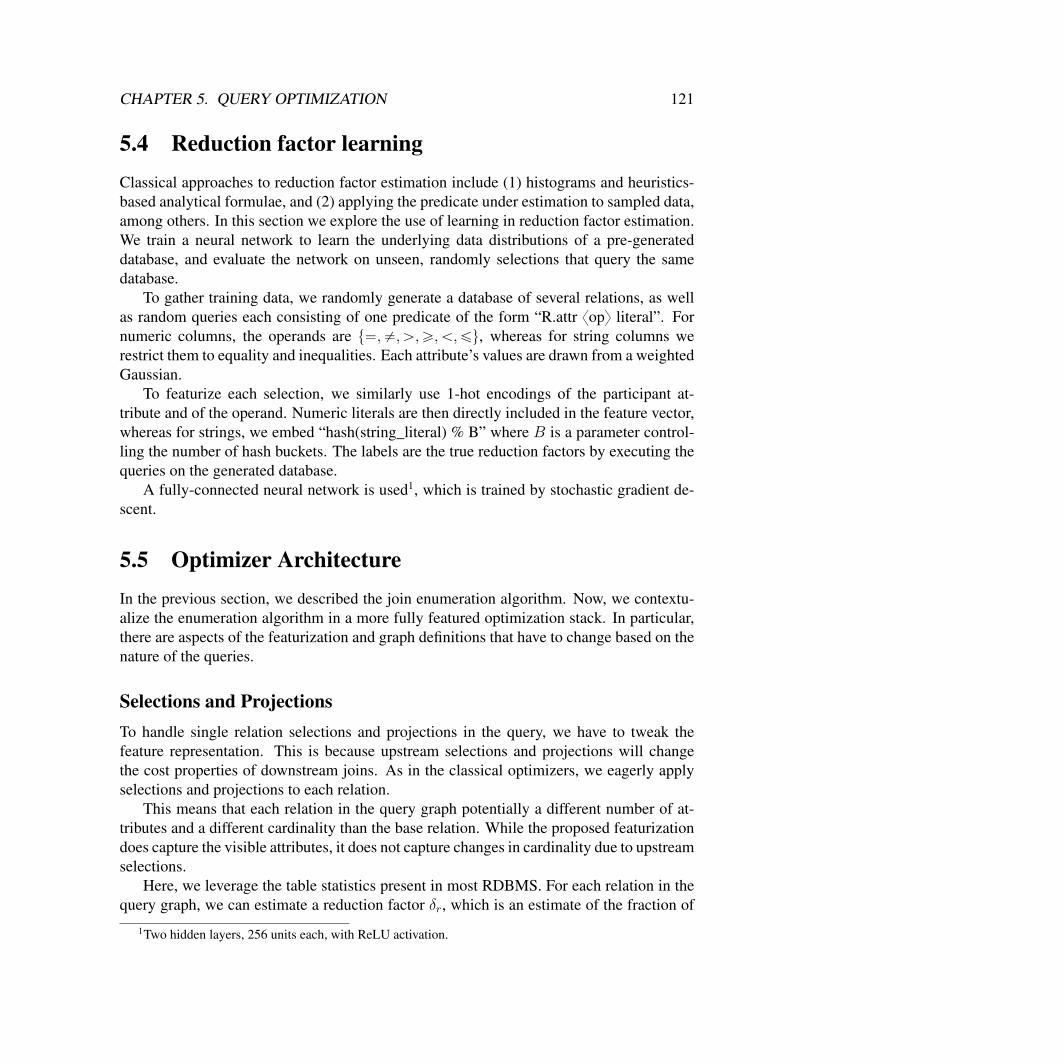
CHAPTER 5. QUERY OPTIMIZATION 121
5.4 Reduction factor learningClassical approaches to reduction factor estimation include (1) histograms and heuristics-based analytical formulae, and (2) applying the predicate under estimation to sampled data,among others. In this section we explore the use of learning in reduction factor estimation.We train a neural network to learn the underlying data distributions of a pre-generateddatabase, and evaluate the network on unseen, randomly selections that query the samedatabase.
To gather training data, we randomly generate a database of several relations, as wellas random queries each consisting of one predicate of the form “R.attr xopy literal”. Fornumeric columns, the operands are t“,‰,ą,ě,ă,ďu, whereas for string columns werestrict them to equality and inequalities. Each attribute’s values are drawn from a weightedGaussian.
To featurize each selection, we similarly use 1-hot encodings of the participant at-tribute and of the operand. Numeric literals are then directly included in the feature vector,whereas for strings, we embed “hash(string_literal) % B” where B is a parameter control-ling the number of hash buckets. The labels are the true reduction factors by executing thequeries on the generated database.
A fully-connected neural network is used1, which is trained by stochastic gradient de-scent.
5.5 Optimizer ArchitectureIn the previous section, we described the join enumeration algorithm. Now, we contextu-alize the enumeration algorithm in a more fully featured optimization stack. In particular,there are aspects of the featurization and graph definitions that have to change based on thenature of the queries.
Selections and ProjectionsTo handle single relation selections and projections in the query, we have to tweak thefeature representation. This is because upstream selections and projections will changethe cost properties of downstream joins. As in the classical optimizers, we eagerly applyselections and projections to each relation.
This means that each relation in the query graph potentially a different number of at-tributes and a different cardinality than the base relation. While the proposed featurizationdoes capture the visible attributes, it does not capture changes in cardinality due to upstreamselections.
Here, we leverage the table statistics present in most RDBMS. For each relation in thequery graph, we can estimate a reduction factor δr, which is an estimate of the fraction of
1Two hidden layers, 256 units each, with ReLU activation.
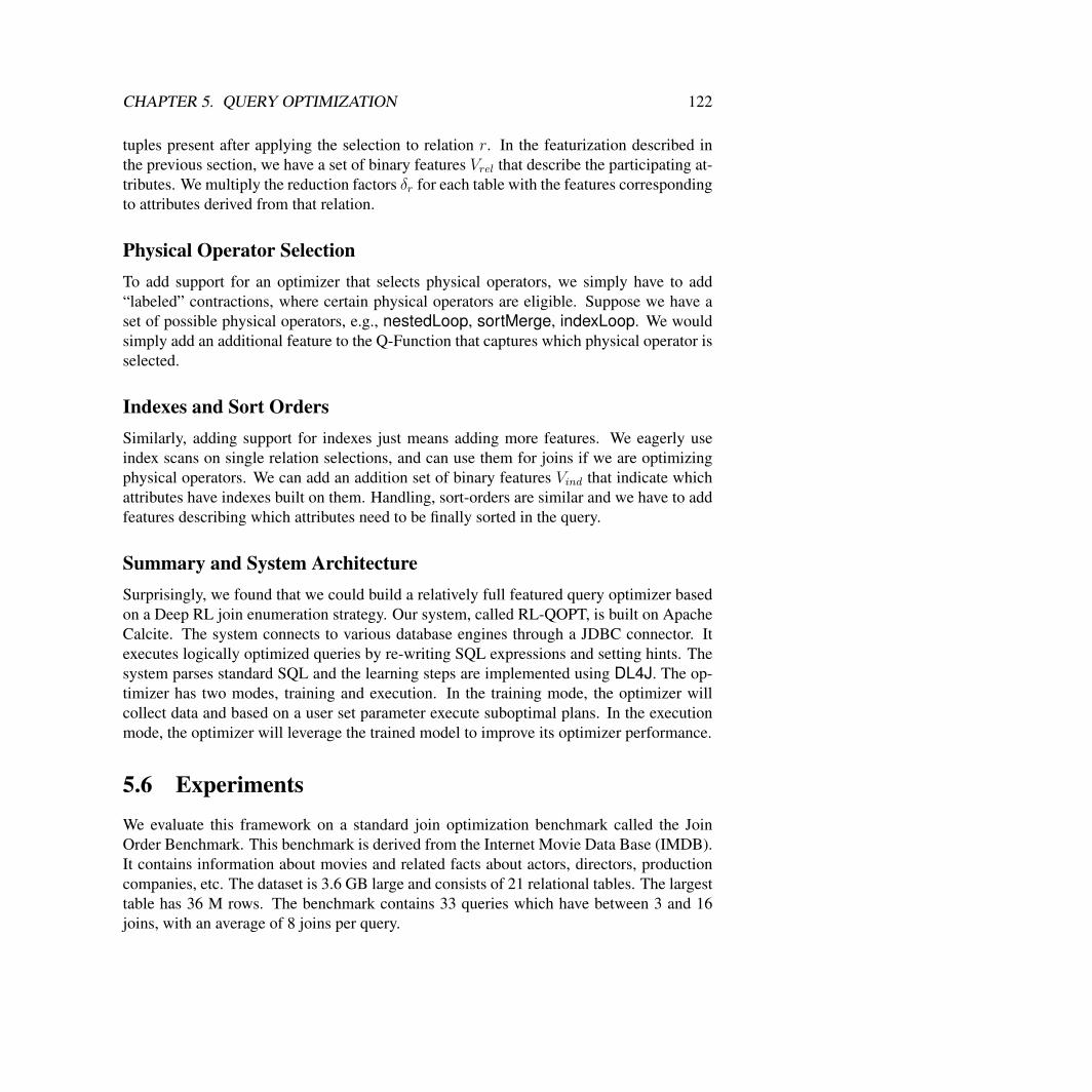
CHAPTER 5. QUERY OPTIMIZATION 122
tuples present after applying the selection to relation r. In the featurization described inthe previous section, we have a set of binary features Vrel that describe the participating at-tributes. We multiply the reduction factors δr for each table with the features correspondingto attributes derived from that relation.
Physical Operator SelectionTo add support for an optimizer that selects physical operators, we simply have to add“labeled” contractions, where certain physical operators are eligible. Suppose we have aset of possible physical operators, e.g., nestedLoop, sortMerge, indexLoop. We wouldsimply add an additional feature to the Q-Function that captures which physical operator isselected.
Indexes and Sort OrdersSimilarly, adding support for indexes just means adding more features. We eagerly useindex scans on single relation selections, and can use them for joins if we are optimizingphysical operators. We can add an addition set of binary features Vind that indicate whichattributes have indexes built on them. Handling, sort-orders are similar and we have to addfeatures describing which attributes need to be finally sorted in the query.
Summary and System ArchitectureSurprisingly, we found that we could build a relatively full featured query optimizer basedon a Deep RL join enumeration strategy. Our system, called RL-QOPT, is built on ApacheCalcite. The system connects to various database engines through a JDBC connector. Itexecutes logically optimized queries by re-writing SQL expressions and setting hints. Thesystem parses standard SQL and the learning steps are implemented using DL4J. The op-timizer has two modes, training and execution. In the training mode, the optimizer willcollect data and based on a user set parameter execute suboptimal plans. In the executionmode, the optimizer will leverage the trained model to improve its optimizer performance.
5.6 ExperimentsWe evaluate this framework on a standard join optimization benchmark called the JoinOrder Benchmark. This benchmark is derived from the Internet Movie Data Base (IMDB).It contains information about movies and related facts about actors, directors, productioncompanies, etc. The dataset is 3.6 GB large and consists of 21 relational tables. The largesttable has 36 M rows. The benchmark contains 33 queries which have between 3 and 16joins, with an average of 8 joins per query.
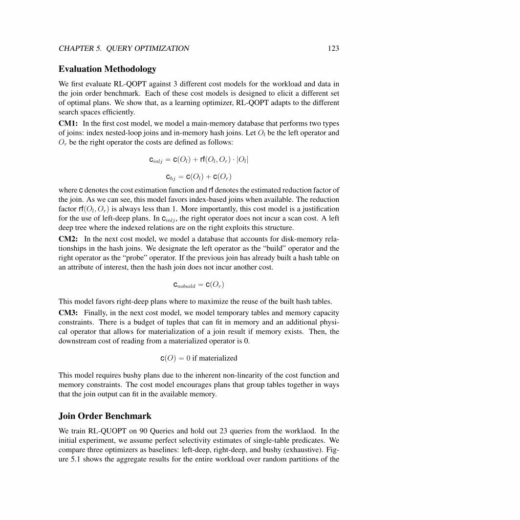
CHAPTER 5. QUERY OPTIMIZATION 123
Evaluation MethodologyWe first evaluate RL-QOPT against 3 different cost models for the workload and data inthe join order benchmark. Each of these cost models is designed to elicit a different setof optimal plans. We show that, as a learning optimizer, RL-QOPT adapts to the differentsearch spaces efficiently.CM1: In the first cost model, we model a main-memory database that performs two typesof joins: index nested-loop joins and in-memory hash joins. Let Ol be the left operator andOr be the right operator the costs are defined as follows:
cinlj “ cpOlq ` rfpOl, Orq ¨ |Ol|
chj “ cpOlq ` cpOrq
where c denotes the cost estimation function and rf denotes the estimated reduction factor ofthe join. As we can see, this model favors index-based joins when available. The reductionfactor rfpOl, Orq is always less than 1. More importantly, this cost model is a justificationfor the use of left-deep plans. In cinlj , the right operator does not incur a scan cost. A leftdeep tree where the indexed relations are on the right exploits this structure.CM2: In the next cost model, we model a database that accounts for disk-memory rela-tionships in the hash joins. We designate the left operator as the “build” operator and theright operator as the “probe” operator. If the previous join has already built a hash table onan attribute of interest, then the hash join does not incur another cost.
cnobuild “ cpOrq
This model favors right-deep plans where to maximize the reuse of the built hash tables.CM3: Finally, in the next cost model, we model temporary tables and memory capacityconstraints. There is a budget of tuples that can fit in memory and an additional physi-cal operator that allows for materialization of a join result if memory exists. Then, thedownstream cost of reading from a materialized operator is 0.
cpOq “ 0 if materialized
This model requires bushy plans due to the inherent non-linearity of the cost function andmemory constraints. The cost model encourages plans that group tables together in waysthat the join output can fit in the available memory.
Join Order BenchmarkWe train RL-QUOPT on 90 Queries and hold out 23 queries from the worklaod. In theinitial experiment, we assume perfect selectivity estimates of single-table predicates. Wecompare three optimizers as baselines: left-deep, right-deep, and bushy (exhaustive). Fig-ure 5.1 shows the aggregate results for the entire workload over random partitions of the
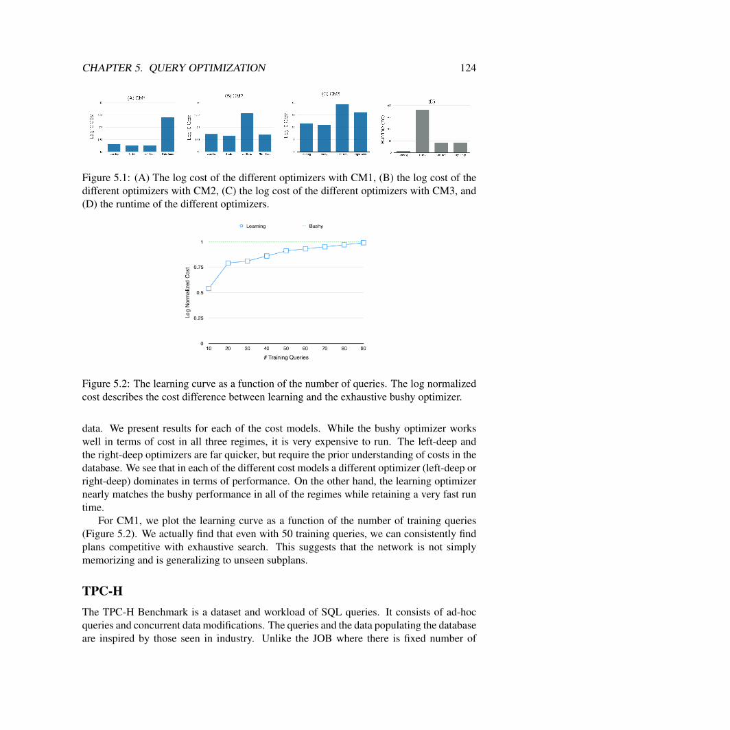
CHAPTER 5. QUERY OPTIMIZATION 124
Figure 5.1: (A) The log cost of the different optimizers with CM1, (B) the log cost of thedifferent optimizers with CM2, (C) the log cost of the different optimizers with CM3, and(D) the runtime of the different optimizers.
Figure 5.2: The learning curve as a function of the number of queries. The log normalizedcost describes the cost difference between learning and the exhaustive bushy optimizer.
data. We present results for each of the cost models. While the bushy optimizer workswell in terms of cost in all three regimes, it is very expensive to run. The left-deep andthe right-deep optimizers are far quicker, but require the prior understanding of costs in thedatabase. We see that in each of the different cost models a different optimizer (left-deep orright-deep) dominates in terms of performance. On the other hand, the learning optimizernearly matches the bushy performance in all of the regimes while retaining a very fast runtime.
For CM1, we plot the learning curve as a function of the number of training queries(Figure 5.2). We actually find that even with 50 training queries, we can consistently findplans competitive with exhaustive search. This suggests that the network is not simplymemorizing and is generalizing to unseen subplans.
TPC-HThe TPC-H Benchmark is a dataset and workload of SQL queries. It consists of ad-hocqueries and concurrent data modifications. The queries and the data populating the databaseare inspired by those seen in industry. Unlike the JOB where there is fixed number of
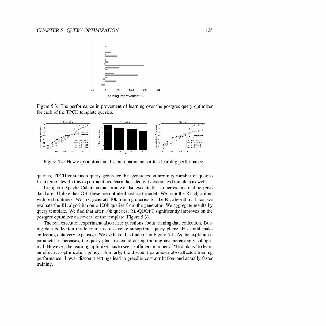
CHAPTER 5. QUERY OPTIMIZATION 125
Learning Improvement %-75 0 75 150 225 300
Figure 5.3: The performance improvement of learning over the postgres query optimizerfor each of the TPCH template queries.
Figure 5.4: How exploration and discount parameters affect learning performance.
queries, TPCH contains a query generator that generates an arbitrary number of queriesfrom templates. In this experiment, we learn the selectivity estimates from data as well.
Using our Apache Calcite connection, we also execute these queries on a real postgresdatabase. Unlike the JOB, these are not idealized cost model. We train the RL algorithmwith real runtimes. We first generate 10k training queries for the RL algorithm. Then, weevaluate the RL algorithm on a 100k queries from the generator. We aggregate results byquery template. We find that after 10k queries, RL-QUOPT significantly improves on thepostgres optimizer on several of the template (Figure 5.3).
The real execution experiment also raises questions about training data collection. Dur-ing data collection the learner has to execute suboptimal query plans; this could makecollecting data very expensive. We evaluate this tradeoff in Figure 5.4. As the explorationparameter ε increases, the query plans executed during training are increasingly subopti-mal. However, the learning optimizer has to see a sufficient number of “bad plans” to learnan effective optimization policy. Similarly, the discount parameter also affected trainingperformance. Lower discount settings lead to greedier cost attribution–and actually fastertraining.

CHAPTER 5. QUERY OPTIMIZATION 126
ConclusionReinforcement learning introduces a new approximate dynamic programming frameworkfor SQL query optimization. Classical query optimizers leverage dynamic programs foroptimally nesting join queries. This process creates a table that memoizes cost-to-go es-timates of intermediate subplans. By representing the memoization table with a neuralnetwork, the optimizer can estimate the cost-to-go of even previously unseen plans allow-ing for a vast expansion of the search space. I show that this process is a form of DeepQ-Learning where the state is a query graph and the actions are contractions on the querygraph. One key result is that the same optimization algorithm can adaptively learn searchstrategies for both in-memory databases (where the search space is often heuristically re-stricted based to maximize index accesses) and disk-based databases (where the searchspace is often heuristically restricted to maximize re-use of intermediate results).

Chapter 6
Reinforcement Learning forSurgical Tensioning
Robotic surgical assistants (RSAs), such as Intuitive Surgical’s da Vinci, facilitate preciseminimally invasive surgery [129]. These robots currently operate under pure tele-operationcontrol, but introducing assistive autonomy has potential to improve surgical training, as-sist surgeons, reduce fatigue, and facilitate tele-surgery. For example, when cutting thintissue with surgical scissors, a surgeon may use a second or even a third tool to pin downand fixture the tissue. This technique, called tensioning (also called traction), adds addi-tional constraints on the material to prevent deformations during the cutting from drasticallychanging the position of the desired cutting path. The optimal direction and magnitude ofthe tensioning force changes as the cutting progresses, and these forces must adapt to anydeformations that occur. However, practically, the surgeon’s tensioning policy is often sub-optimal because: (1) surgeon can automatically manipulate only two of the tools at onceleaving any third arm stationary, and (2) asymmetric multilateral tasks (arms doing differentprocedures) are known to be challenging without significant training with the tele-operativesystem.
Therefore, it would be beneficial to automatically synthesize tensioning policies to bestassist an open loop cutting trajectory. The first challenge is modeling the dynamics ofcutting and tensioning. One way to model deformable sheets is with a 3-dimensional mass-spring-damper network. A sheet is a planar graph of point masses connected by dampedsprings at edges. k of the point masses are constrained to be fixed at a particular 3Dlocation, i.e., they are tensioned, and the positions of the remaining masses is determinedby the dynamics induced these constraints. At each time step, the constraint can be movedto a new location. Cutting is modeled by removing a single edge in the graph at each time-step. For k assistive arms, the optimization objective is to plan sequence of k movableboundary value constraints to maximize cutting accuracy.
This problem constitutes a highly non-convex optimal control problem, whether cut-ting accuracy is a non-convex objective that measures the symmetric difference between a
127
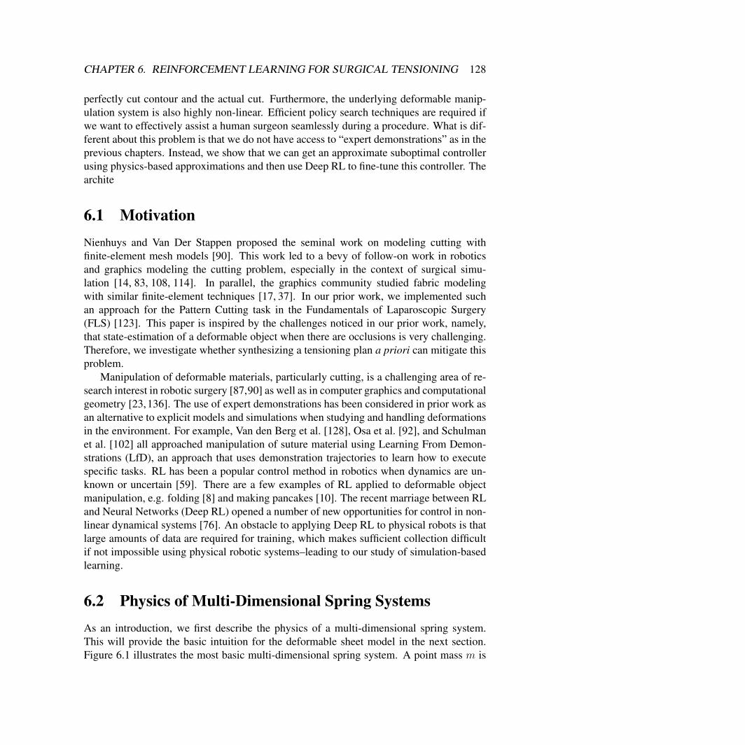
CHAPTER 6. REINFORCEMENT LEARNING FOR SURGICAL TENSIONING 128
perfectly cut contour and the actual cut. Furthermore, the underlying deformable manip-ulation system is also highly non-linear. Efficient policy search techniques are required ifwe want to effectively assist a human surgeon seamlessly during a procedure. What is dif-ferent about this problem is that we do not have access to “expert demonstrations” as in theprevious chapters. Instead, we show that we can get an approximate suboptimal controllerusing physics-based approximations and then use Deep RL to fine-tune this controller. Thearchite
6.1 MotivationNienhuys and Van Der Stappen proposed the seminal work on modeling cutting withfinite-element mesh models [90]. This work led to a bevy of follow-on work in roboticsand graphics modeling the cutting problem, especially in the context of surgical simu-lation [14, 83, 108, 114]. In parallel, the graphics community studied fabric modelingwith similar finite-element techniques [17, 37]. In our prior work, we implemented suchan approach for the Pattern Cutting task in the Fundamentals of Laparoscopic Surgery(FLS) [123]. This paper is inspired by the challenges noticed in our prior work, namely,that state-estimation of a deformable object when there are occlusions is very challenging.Therefore, we investigate whether synthesizing a tensioning plan a priori can mitigate thisproblem.
Manipulation of deformable materials, particularly cutting, is a challenging area of re-search interest in robotic surgery [87,90] as well as in computer graphics and computationalgeometry [23,136]. The use of expert demonstrations has been considered in prior work asan alternative to explicit models and simulations when studying and handling deformationsin the environment. For example, Van den Berg et al. [128], Osa et al. [92], and Schulmanet al. [102] all approached manipulation of suture material using Learning From Demon-strations (LfD), an approach that uses demonstration trajectories to learn how to executespecific tasks. RL has been a popular control method in robotics when dynamics are un-known or uncertain [59]. There are a few examples of RL applied to deformable objectmanipulation, e.g. folding [8] and making pancakes [10]. The recent marriage between RLand Neural Networks (Deep RL) opened a number of new opportunities for control in non-linear dynamical systems [76]. An obstacle to applying Deep RL to physical robots is thatlarge amounts of data are required for training, which makes sufficient collection difficultif not impossible using physical robotic systems–leading to our study of simulation-basedlearning.
6.2 Physics of Multi-Dimensional Spring SystemsAs an introduction, we first describe the physics of a multi-dimensional spring system.This will provide the basic intuition for the deformable sheet model in the next section.Figure 6.1 illustrates the most basic multi-dimensional spring system. A point mass m is

CHAPTER 6. REINFORCEMENT LEARNING FOR SURGICAL TENSIONING 129
Figure 6.1: This illustration describes a basic mass-spring-damper system with spring con-stant k and damping constant c.
connected by a spring and damper to a infinitely strong block T . The spring constant is k(let ` denote the resting length) and the damping constant is c. Let denote the accelerationvector a “ r:x :y :zsT of the point mass:
ma “ Fspring ` Fdamper.
Hooke’s law states that the magnitude of the force applied by a spring is proportional to itsdeviation D from the rest length:
|Fspring| “ kD.
Using unit vector notation, we can parametrize the force vector with spherical coordinates:
Fspring “ i kpD ´ `q sin θ cosψ ` j kpD ´ `q sin θ sinψ ` k kpD ´ `q cos θ
where D “a
px´ Txq2 ` py ´ Tyq2 ` pz ´ Tzq2, θ “ cos´1 pz´TzqD
, ψ “ tan´1 py´Tyq
px´Txq.
For the damper, let v “ r 9x 9y 9zsT denote the velocity vector:
Fdamper “ cv.
The resulting equations of motion are:
ma “ i pkpD ´ `q sin θ cosψ ` cvxq ` j pkpD ´ `q sin θ sinψ ` cvyq ` k pkpD ´ `q cos θ ` cvzq. (6)
Simulator
We can use this model to design a simulator for cutting deformable sheets. LetGx,y,z Ă R3
be a three-dimensional global coordinate frame. We denote the set of points on this sheet

CHAPTER 6. REINFORCEMENT LEARNING FOR SURGICAL TENSIONING 130
as Σ, and ΣpGq is the locations of these points in the global frame. The points are connectedby a graph of springs and dampers. To apply the above equation of motion, we can treateach neighboring vertex as a wall. For each p P Σ, the neighboring vertex q P Nppq appliesa force Fpq. Cutting is modeled as removing an edge from the graph. In this paper, weassume that all of the springs have the same constant, natural length, and all the dampingconstants are the same.
The simulator is initialized with some initial state ΣpGq0 P Gx,y,z. The state is then
iteratively updated based on the derived equations of motion above. For each p P Σ, theupdates have the following form:
m:p “ÿ
qPNppq
Fpq ` Fexternal (7)
To update the position p, we use the implicit Adams method with a standard python toolkit1. Tensioning is simulated as a position constraint for a chosen pinch point p1 P Σ:
p1 “ u
This means that regardless of the forces applied to this point it will remain at position u.
Manipulation ActionsWe are given a rectangular planar sheet and a simple algebraic desired cutting contour ofbounded curvature, which can be either closed or open.
Cutting
We assume that one arm of the robot is designated as the cutting arm and the other as thetensioning arm. A cutting contour is a sequence of points C on the surface of the sheet. Thecutting arm operates in an open-loop trajectory that attempts to cut alongC0, the position ofthe cutting contour in the global frame at time zero. Error is measured using the symmetricdifference between the desired contour on the sheet and the achieved contour cut. Thesewill be different due to deformation of the sheet during cutting. Let X be the set of pointsinside a closed intended trajectory and let Y be the set of points inside a closed simulatedtrajectory. The symmetric difference is then the exclusive-or A ‘ B of the two sets. Foropen contours, the contours are closed by forming boundaries with the edges of the sheet.
Tensioning
Since the cutting is open-loop it cannot account for deformation, and this is why we needtensioning to apply feedback based on the state of the sheet.
1https://docs.scipy.org/doc/scipy-0.14.0/reference/generated/scipy.integrate.ode.html
CHAPTER 6. REINFORCEMENT LEARNING FOR SURGICAL TENSIONING 131
Definition 7 (Tensioning) Let s P Σ be called a pinch point. Tensioning is defined asconstraining the position of this pinch point to a specific location u P Gx,y,z:
T “ xs, uy
For each of the k tensioning arms of the robot, we can have one tuple Ti. We considera single pinch point for each arm for an entire cutting trajectory. This allows us to define atensioning policy:
Definition 8 (Tensioning Policy) For arm i P t1, .., ku, let ΣpGqt be the locations of all of
the points on the sheet in the global coordinate frame at time t. For a fixed pinch point s, atensioning policy πs is a function where ∆u “ ut`1 ´ ut:
πi : ΣpGqptq ÞÑ ∆u
Problem. Tensioning Policy Search: For each arm i, find a tensioning policy that mini-mizes the symmetric difference of the desired vs. actual contour.
6.3 Reinforcement Learning For Policy SearchWe chose an RL algorithm since the symmetric difference reward function is non-convexand the system in non-linear. We model the tensioning problem as a Markov DecisionProcess (MDP):
xS,A, ξp¨, ¨q, Rp¨, ¨q, T y.
where the actions A are 1mm movements of the tensioning arm in the x and y directions,and the states S are described below. The action space is tuned so the policy can generatesufficient tension to manipulate the cloth significantly over a few timesteps. Reward ismeasured using the symmetric difference between the desired contour and the achievedcontour cut. The robot receives 0 reward at all time-steps prior to the last step, and at thelast time-step T ´ 1 receives the symmetric difference. We do not shape the reward, assymmetric difference is exactly the error metric used for evaluation as well.
To optimize θ, we leverage the TRPO implementation [103] in Rllab [32]. We use aneural network to parametrize the policy πθ, which maps an observation vector to a dis-crete action. A two 32x32 Hidden Layer Multi-Layer Perceptron is used to represent thismapping. Since neural networks are differentiable, we can optimize the quantity Rpθq.The state space is a tuple consisting of the time index of the trajectory t, the displacementvector from the original pinch point ut, and the location xi P R3 of fiducial points chosenrandomly on the surface of the sheet. In all experiments we use 12 fiducial points. This isa sample-based approximation of tracking Σ
pGqt .
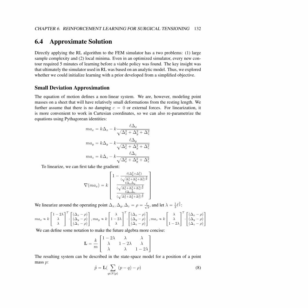
CHAPTER 6. REINFORCEMENT LEARNING FOR SURGICAL TENSIONING 132
6.4 Approximate SolutionDirectly applying the RL algorithm to the FEM simulator has a two problems: (1) largesample complexity and (2) local minima. Even in an optimized simulator, every new con-tour required 5 minutes of learning before a viable policy was found. The key insight wasthat ultimately the simulator used in RL was based on an analytic model. Thus, we exploredwhether we could initialize learning with a prior developed from a simplified objective.
Small Deviation ApproximationThe equation of motion defines a non-linear system. We are, however, modeling pointmasses on a sheet that will have relatively small deformations from the resting length. Wefurther assume that there is no damping c “ 0 or external forces. For linearization, itis more convenient to work in Cartesian coordinates, so we can also re-parametrize theequations using Pythagorean identities:
max “ k∆x ´ k`∆x
a
∆2x `∆2
y `∆2z
may “ k∆y ´ k`∆y
a
∆2x `∆2
y `∆2z
maz “ k∆z ´ k`∆z
a
∆2x `∆2
y `∆2z
To linearize, we can first take the gradient:
∇pmaxq “ k
»
—
—
—
—
–
1´`p∆2
y`∆2zq
p?
∆2x`∆2
y`∆2zq
32
`∆x∆y
p?
∆2x`∆2
y`∆2zq
32
`∆x∆z
p?
∆2x`∆2
y`∆2zq
32
fi
ffi
ffi
ffi
ffi
fl
We linearize around the operating point ∆x,∆y,∆z “ ρ “ ?3, and let λ “ 1
3`
32 :
max « k
»
–
1´ 2λλλ
fi
fl
T
¨
»
–
p∆x ´ ρqp∆y ´ ρqp∆z ´ ρq
fi
fl ,may « k
»
–
λ1´ 2λλ
fi
fl
T
¨
»
–
p∆x ´ ρqp∆y ´ ρqp∆z ´ ρq
fi
fl ,maz « k
»
–
λλ
1´ 2λ
fi
fl
T
¨
»
–
p∆x ´ ρqp∆y ´ ρqp∆z ´ ρq
fi
fl
We can define some notation to make the future algebra more concise:
L “k
m
»
–
1´ 2λ λ λλ 1´ 2λ λλ λ 1´ 2λ
fi
fl
The resulting system can be described in the state-space model for a position of a pointmass p:
:p “ Lpÿ
qPNppq
pp´ qq ´ ρq (8)
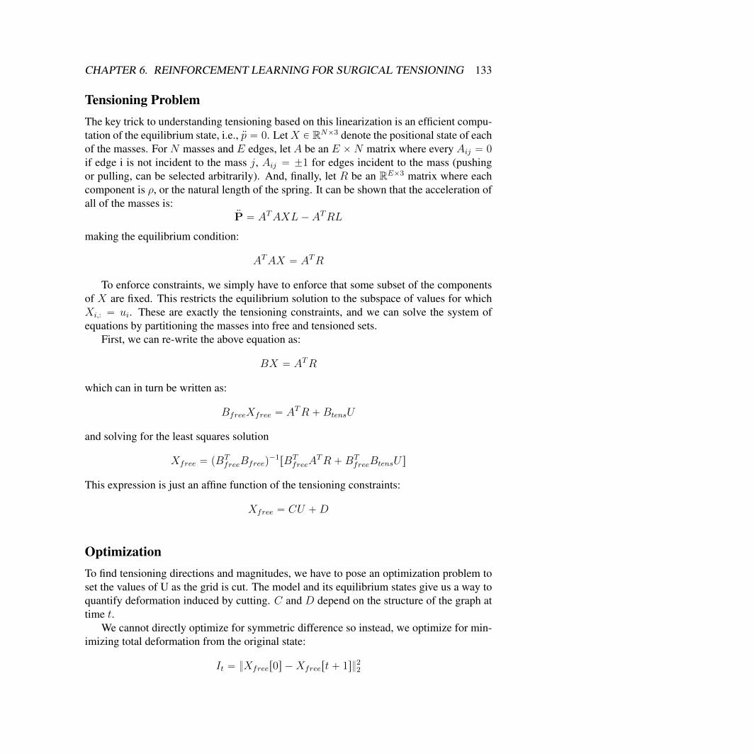
CHAPTER 6. REINFORCEMENT LEARNING FOR SURGICAL TENSIONING 133
Tensioning ProblemThe key trick to understanding tensioning based on this linearization is an efficient compu-tation of the equilibrium state, i.e., :p “ 0. LetX P RNˆ3 denote the positional state of eachof the masses. For N masses and E edges, let A be an E ˆN matrix where every Aij “ 0if edge i is not incident to the mass j, Aij “ ˘1 for edges incident to the mass (pushingor pulling, can be selected arbitrarily). And, finally, let R be an REˆ3 matrix where eachcomponent is ρ, or the natural length of the spring. It can be shown that the acceleration ofall of the masses is:
:P “ ATAXL´ ATRL
making the equilibrium condition:
ATAX “ ATR
To enforce constraints, we simply have to enforce that some subset of the componentsof X are fixed. This restricts the equilibrium solution to the subspace of values for whichXi,: “ ui. These are exactly the tensioning constraints, and we can solve the system ofequations by partitioning the masses into free and tensioned sets.
First, we can re-write the above equation as:
BX “ ATR
which can in turn be written as:
BfreeXfree “ ATR `BtensU
and solving for the least squares solution
Xfree “ pBTfreeBfreeq
´1rBT
freeATR `BT
freeBtensU s
This expression is just an affine function of the tensioning constraints:
Xfree “ CU `D
OptimizationTo find tensioning directions and magnitudes, we have to pose an optimization problem toset the values of U as the grid is cut. The model and its equilibrium states give us a way toquantify deformation induced by cutting. C and D depend on the structure of the graph attime t.
We cannot directly optimize for symmetric difference so instead, we optimize for min-imizing total deformation from the original state:
It “ }Xfreer0s ´Xfreert` 1s}22
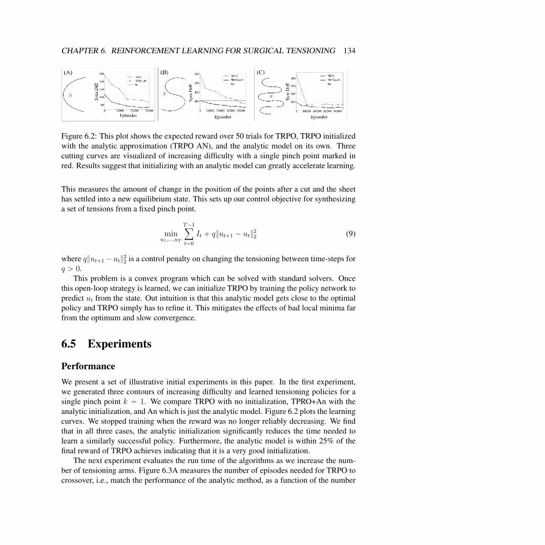
CHAPTER 6. REINFORCEMENT LEARNING FOR SURGICAL TENSIONING 134
Figure 6.2: This plot shows the expected reward over 50 trials for TRPO, TRPO initializedwith the analytic approximation (TRPO AN), and the analytic model on its own. Threecutting curves are visualized of increasing difficulty with a single pinch point marked inred. Results suggest that initializing with an analytic model can greatly accelerate learning.
This measures the amount of change in the position of the points after a cut and the sheethas settled into a new equilibrium state. This sets up our control objective for synthesizinga set of tensions from a fixed pinch point.
minu1,...,uT
T´1ÿ
t“0
It ` q}ut`1 ´ ut}22 (9)
where q}ut`1´ut}22 is a control penalty on changing the tensioning between time-steps for
q ą 0.This problem is a convex program which can be solved with standard solvers. Once
this open-loop strategy is learned, we can initialize TRPO by training the policy network topredict ut from the state. Out intuition is that this analytic model gets close to the optimalpolicy and TRPO simply has to refine it. This mitigates the effects of bad local minima farfrom the optimum and slow convergence.
6.5 Experiments
PerformanceWe present a set of illustrative initial experiments in this paper. In the first experiment,we generated three contours of increasing difficulty and learned tensioning policies for asingle pinch point k “ 1. We compare TRPO with no initialization, TPRO+An with theanalytic initialization, and An which is just the analytic model. Figure 6.2 plots the learningcurves. We stopped training when the reward was no longer reliably decreasing. We findthat in all three cases, the analytic initialization significantly reduces the time needed tolearn a similarly successful policy. Furthermore, the analytic model is within 25% of thefinal reward of TRPO achieves indicating that it is a very good initialization.
The next experiment evaluates the run time of the algorithms as we increase the num-ber of tensioning arms. Figure 6.3A measures the number of episodes needed for TRPO tocrossover, i.e., match the performance of the analytic method, as a function of the number
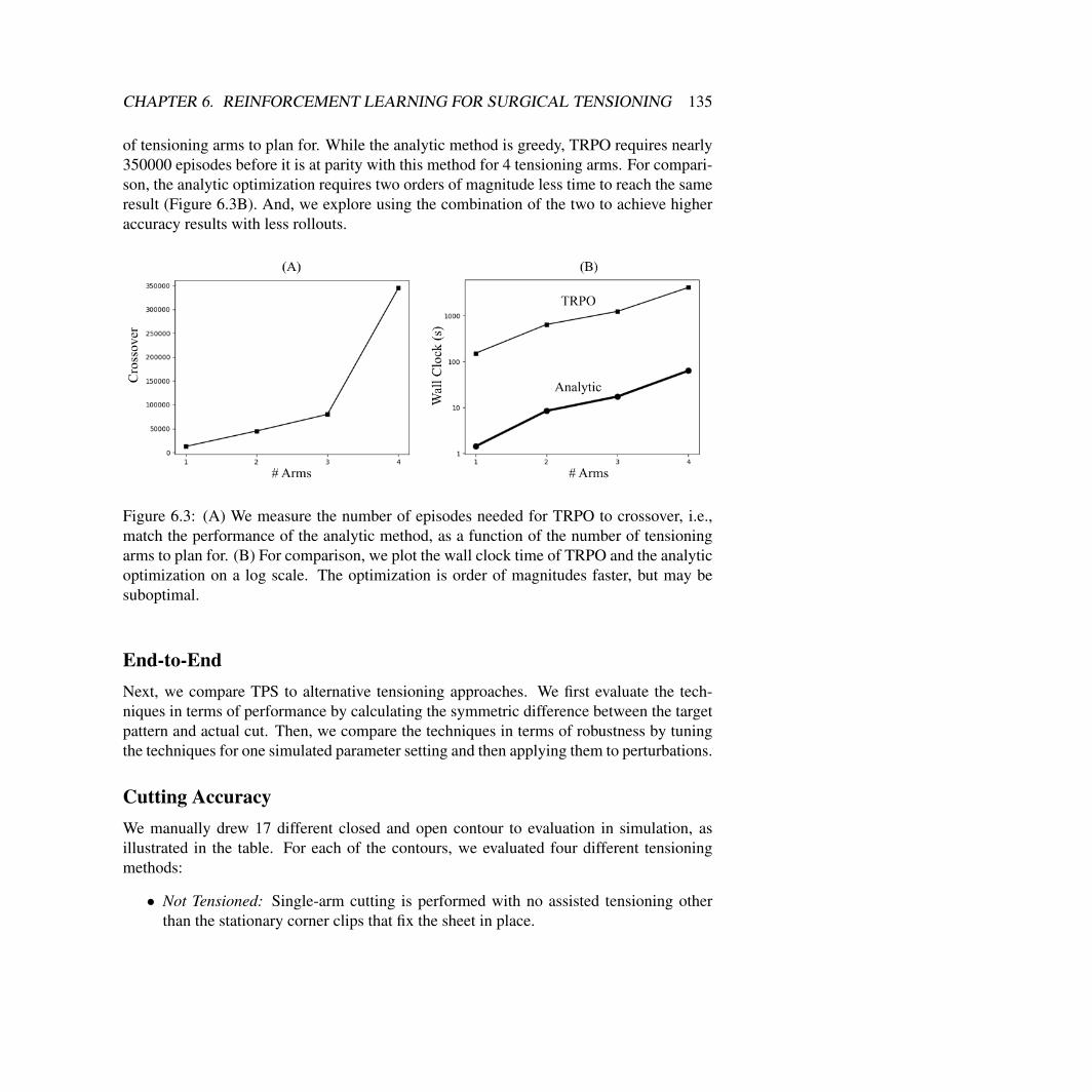
CHAPTER 6. REINFORCEMENT LEARNING FOR SURGICAL TENSIONING 135
of tensioning arms to plan for. While the analytic method is greedy, TRPO requires nearly350000 episodes before it is at parity with this method for 4 tensioning arms. For compari-son, the analytic optimization requires two orders of magnitude less time to reach the sameresult (Figure 6.3B). And, we explore using the combination of the two to achieve higheraccuracy results with less rollouts.
Figure 6.3: (A) We measure the number of episodes needed for TRPO to crossover, i.e.,match the performance of the analytic method, as a function of the number of tensioningarms to plan for. (B) For comparison, we plot the wall clock time of TRPO and the analyticoptimization on a log scale. The optimization is order of magnitudes faster, but may besuboptimal.
End-to-EndNext, we compare TPS to alternative tensioning approaches. We first evaluate the tech-niques in terms of performance by calculating the symmetric difference between the targetpattern and actual cut. Then, we compare the techniques in terms of robustness by tuningthe techniques for one simulated parameter setting and then applying them to perturbations.
Cutting AccuracyWe manually drew 17 different closed and open contour to evaluation in simulation, asillustrated in the table. For each of the contours, we evaluated four different tensioningmethods:
• Not Tensioned: Single-arm cutting is performed with no assisted tensioning otherthan the stationary corner clips that fix the sheet in place.

CHAPTER 6. REINFORCEMENT LEARNING FOR SURGICAL TENSIONING 136
• Fixed Tensioning: The material is pinched at a single point with the gripper arm(with corner points still fixed in place), but no directional tensioning is applied. Wesimulate area contact by pinching a circular disc.
• Centroid Tensioning: Tensioning is proportional to the direction and magnitude ofthe error in the 3D position of the cutting tool and the closest point on the desiredcontour. The gain was hand-tuned on randomly-chosen contours and is fixed to 0.01.
• TPS A separate policy is trained for each shape, this requires 20 iterations of TRPOin the simulator.
For the analytic tensioning model, the centroid of the contour is used as the pinch point.For the fixed policy, the point was chosen by random search over the feasible set of points.Performance is measured using the symmetric difference between the desired contour andthe actual cut.
The averaged symmetric difference scores for each instance and tensioning method arereported in table. The success of the different tensioning algorithms are presented as thepercentage of improvement in symmetric difference score over the non-tensioned baseline.The average of the scores over all 17 contours are also included in the table. For theselected set of contours, TPS achieves the best average relative improvement of 43.30%,the analytical method 9.70%, and the fixed approach 13.54%.
dVRK: Hardware and SoftwareWe use the Intuitive Surgical da Vinci Research Kit (dVRK) surgical robot assistant, asin [40, 87, 105]. We interface with the dVRK using open-source electronics and softwaredeveloped by [56]. The software system is integrated with ROS and allows direct robotpose control. We use the standard laparoscopic stereo camera for tracking fiducials on thesurgical gauze. We equip the right arm with the curved scissors tooltip for cutting and theleft arm with the needle driver tooltip for pinching and tensioning. The arms are located oneither side of the surgical gauze to maximize the workspace for each without collision.
Physical Evaluation of TPSWe show the physical results on 4 contours using Fixed Tensioning and Deep RL using thesymmetric difference as the evaluation metric in table. The tensioning policy for Deep RLwas derived from simulation experiments by registering the physical gauze to a sheet in thesimulator environment. In this set of experiments, we used fixed tensioning as the baseline.The no tensioning policy frequently failed in the physical experiment so we excluded thatfrom the results table for a fair baseline comparison. We were unable to evaluate the ana-lytic method in the physical experiments because the state-estimation needed for feedbackcontrol was not possible outside of the simulated environment.
CHAPTER 6. REINFORCEMENT LEARNING FOR SURGICAL TENSIONING 137
We do not attempt analytic tensioning since it requires real-time tracking of the patternto estimate local error. We observed that 3 out of 4 of the TPS experiments performed bet-ter than the fixed tensioning policy with respect to the symmetric difference of the cut andideal trajectories. This is the same objective the trained policy was designed to minimize insimulation. A weakness of the policy was failure to address discrete failure modes, includ-ing discrete failure modes induced by the policy itself. Failure as a result of the scissors’entanglement in the gauze occurred in both experimental groups. The active manipulationand tensioning of TPS also caused increased deformation of the cloth which occasionallydirectly resulted in entanglement as well. We did not optimize our policy to minimize thesediscrete failures, and our simulator does not model the robot with acceptable fidelity to doso. To address this, we would require very accurate models of the robot arms and tools.
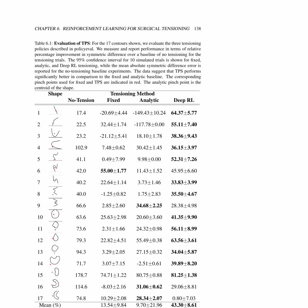
CHAPTER 6. REINFORCEMENT LEARNING FOR SURGICAL TENSIONING 138
Table 6.1: Evaluation of TPS: For the 17 contours shown, we evaluate the three tensioningpolicies described in policyeval. We measure and report performance in terms of relativepercentage improvement in symmetric difference over a baseline of no tensioning for thetensioning trials. The 95% confidence interval for 10 simulated trials is shown for fixed,analytic, and Deep RL tensioning, while the mean absolute symmetric difference error isreported for the no-tensioning baseline experiments. The data suggest that TPS performssignificantly better in comparison to the fixed and analytic baseline. The correspondingpinch points used for fixed and TPS are indicated in red. The analytic pinch point is thecentroid of the shape.
Shape Tensioning MethodNo-Tension Fixed Analytic Deep RL
1 17.4 -20.69˘4.44 -149.43˘10.24 64.37˘5.77
2 22.5 32.44˘1.74 -117.78˘0.00 55.11˘7.40
3 23.2 -21.12˘5.41 18.10˘1.78 38.36˘9.43
4 102.9 7.48˘0.62 30.42˘1.45 36.15˘3.97
5 41.1 0.49˘7.99 9.98˘0.00 52.31˘7.26
6 42.0 55.00˘1.77 11.43˘1.52 45.95˘6.60
7 40.2 22.64˘1.14 3.73˘1.46 33.83˘3.99
8 40.0 -1.25˘0.82 1.75˘2.83 35.50˘4.67
9 66.6 2.85˘2.60 34.68˘2.25 28.38˘4.98
10 63.6 25.63˘2.98 20.60˘3.60 41.35˘9.90
11 73.6 2.31˘1.66 24.32˘0.98 56.11˘8.99
12 79.3 22.82˘4.51 55.49˘0.38 63.56˘3.61
13 94.3 3.29˘2.05 27.15˘0.32 34.04˘5.87
14 71.7 3.07˘7.15 -2.51˘0.61 39.89˘8.20
15 178.7 74.71˘1.22 80.75˘0.88 81.25˘1.38
16 114.6 -8.03˘2.16 31.06˘0.62 29.06˘8.81
17 74.8 10.29˘2.08 28.34˘2.07 0.80˘7.03Mean (%) 13.54˘9.84 9.70˘21.96 43.30˘8.61
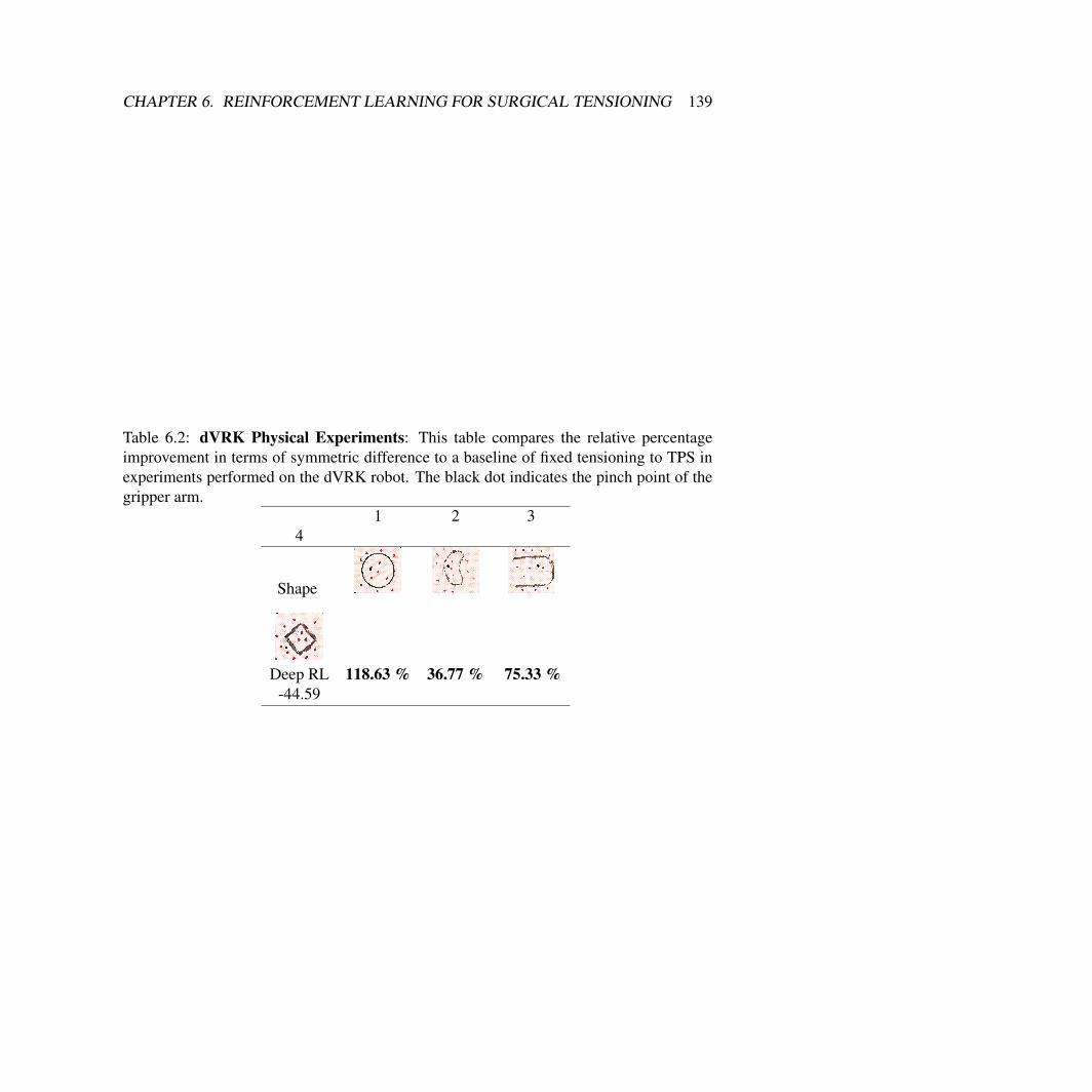
CHAPTER 6. REINFORCEMENT LEARNING FOR SURGICAL TENSIONING 139
Table 6.2: dVRK Physical Experiments: This table compares the relative percentageimprovement in terms of symmetric difference to a baseline of fixed tensioning to TPS inexperiments performed on the dVRK robot. The black dot indicates the pinch point of thegripper arm.
1 2 34
Shape
Deep RL 118.63 % 36.77 % 75.33 %-44.59
Chapter 7
Conclusion
This dissertation explores reinforcement learning, a family of algorithms for finding solu-tions to MDP that assume query access to the underlying dynamical system:
qt : st, at Ñ system() Ñ st`1, rt
High-dimensional and long-horizon search problems can require a prohibitive number ofsuch queries, and exploiting prior knowledge is crucial. In several domains of interest,a limited amount of expert knowledge is available and my dissertation presents an argu-ment learning such structure can significantly improve the sample-efficiency, stability, androbustness of RL methods. With this additional supervision, the search process can be re-stricted to those sequences that are similar to the supervision provided by the expert. Thedissertation explores several Deep RL systems for control of imprecise cable-driven sur-gical robots, automatically synthesizing data-cleaning programs to meet quality specifica-tions, and generating efficient execution plans for relational queries. I describe algorithmiccontributions, theoretical analysis about the implementations themselves, and the architec-ture of the RL systems.
7.1 Challenges and Open ProblemsThe promise of (deep) reinforcement learning is a general algorithm that applies to a largevariety of MDP settings. My dissertation focuses on the RL setting with the most minimalassumptions on the MDP. In general, there is a spectrum of assumptions one could makeand interesting sub-families of algorithms arise at different points on the spectrum.
A Vision For Reinforcement LearningI believe that role of Reinforcement Learning is analagous to the role of Stochastic Gra-dient Descent in supervised learning problems. While it is not practical to expect that RL
140
CHAPTER 7. CONCLUSION 141
will solve every MDP in the most efficient way, we would like it to be competitive to spe-cialized algorithms. This is similar to SGD in many supervised learning problems, whilespecial case alterative exist that are often more performant (e.g., SDCA for SVM problemsand Newton’s Method for Linear Regression), SGD is a reasonable general purpose frame-work that works decently well across a variety of problems. This unification has allowedthe community to build optimized frameworks around SGD, e.g., TensorFlow, and has ul-timately, greatly accelerated the rate of applications research using supervised learning. Ienvision a similar future for RL, one where a small number of RL algorithms are essentiallycompetitive with classical baselines. Better alternatives may exist in special cases but onecan expect RL to work across problem domains. This requires that RL exploit much of thesame problem structure that the classical algorithms exploit.
Reset AssumptionsOne assumption not discussed in this work is how the system can be reset to its initial stateafter querying it. In many problems, one has arbitrary control over the reset process, i.e.,the system can be initialized in any state. This is the principle of backtracking search inconstraint satisfaction and graph search. Designing RL algorithms that intelligently selectinitial states to begin their search is an interesting avenue of research. For example, onecould imagine a Deep Q-Learning learning algorithm which rather than sampling fromthe initial state distribution begins its rollouts from a random point in a trajectory in itsreplay buffer. This would simulate some level of backtracking behavior in the algorithm.Optimizing the initialization process over a collection of tasks would be very valuable.
Distance AssumptionsAnother crucial assumption exploited in many discrete search settings is a priori knowledgeof distance between states. For example, the A* search algorithm uses this to prioritize ex-pansion with an admissible heuristic that lower bounds the cost-to-go. This is functionallyequivalent to a lower bound on the Q-function in RL. An interesting problem is techniquesto learn such lower bounds and transfer them between problems. For example, are thereways to distill a Q network into a simpler model that simply provides a lower approxima-tion and share that with other search problem instances.
Demonstration AssumptionsState-action sequences are the most basic form of supervision from an expert. A moreadvanced expert may be able to provide much more information such as task segments,hierarchical information, and perhaps even hints to the learner. Thinking about how toformalize the notion of hints from the supervisor is another interesting research direction.What if the supervisor could give a partially written program to the describe the control
CHAPTER 7. CONCLUSION 142
policy and the search algorithm could fill in the gaps? There are interesting questions ofhow we represent partial or incomplete knowledge in a framework like RL.
TransferThe “holy grail” of Deep Reinforcement Learning is to demonstrate non-trivial transferof learned policies between MDPs or perturbations of the system. Ensuring safe policydeployments involves understanding the effects of applying a policy trained in simulationor in a training environment to the non-idealities of the real world. For example, in ourquery optimization project, to deploy the policies trained from a cost model, we had toperform significant fine-tuning in the real world.
The challenge is that real world observations often have very different properties thanthe data seen in training. When we execute an SQL query, we do not observe all of the in-termediate costs without significant instrumentation of the database. We may only observea final runtime (the simulator is a proxy for this). Executing subplans can be very expensive(queries can take several minutes to run). However, we can still leverage a final runtimeto adjust plans that optimize runtime, while still leveraging what we have learned from thecost-model. One can think about the fine-tuning process as first using the cost model tolearn relevant features about the structure of subplans (i.e., which ones are generally ben-eficial). After this is learned, those features are fed into a predictor to project the effect ofthat decision on final runtime. Generalizing such ideas is an interesting avenue of research.Can Deep RL in a simulator be used to learn features, which allow for rapid transfer to thereal world?

Bibliography
[1] Trifacta. https://www.trifacta.com/.
[2] Pieter Abbeel and Andrew Y Ng. Apprenticeship learning via inverse reinforcementlearning. In ICML, page 1. ACM, 2004.
[3] Pieter Abbeel and Andrew Y Ng. Inverse reinforcement learning. In Encyclopediaof machine learning, pages 554–558. Springer, 2011.
[4] Tamim Asfour, Pedram Azad, Florian Gyarfas, and Rüdiger Dillmann. Imita-tion learning of dual-arm manipulation tasks in humanoid robots. I. J. HumanoidRobotics, 5(2):183–202, 2008.
[5] Pierre-Luc Bacon, Jean Harb, and Doina Precup. The option-critic architecture.arXiv preprint arXiv:1609.05140, 2016.
[6] Pierre-Luc Bacon and Doina Precup. Learning with options: Just deliberate andrelax. In NIPS Bounded Optimality and Rational Metareasoning Workshop, 2015.
[7] Peter Bailis, Deepak Narayanan, and Samuel Madden. Macrobase: Analytic moni-toring for the internet of things. In arXiv, 2016.
[8] Benjamin Balaguer and Stefano Carpin. Combining imitation and reinforcementlearning to fold deformable planar objects. In 2011 IEEE/RSJ International Confer-ence on Intelligent Robots and Systems, pages 1405–1412. IEEE, 2011.
[9] Andrew G. Barto and Sridhar Mahadevan. Recent advances in hierarchical rein-forcement learning. Discrete Event Dynamic Systems, 13(1-2):41–77, 2003.
[10] Michael Beetz, Ulrich Klank, Ingo Kresse, Alexis Maldonado, Lorenz Mösenlech-ner, Dejan Pangercic, Thomas Rühr, and Moritz Tenorth. Robotic roommates mak-ing pancakes. In Humanoids, pages 529–536. IEEE, 2011.
[11] Richard Bellman. Dynamic programming. Princeton University Press, 1957.
[12] Michael Benedikt, George Konstantinidis, Giansalvatore Mecca, Boris Motik, PaoloPapotti, Donatello Santoro, and Efthymia Tsamoura. Benchmarking the chase. InPODS, 2017.
143
BIBLIOGRAPHY 144
[13] Dimitri P Bertsekas and John N Tsitsiklis. Neuro-dynamic programming: anoverview. In Decision and Control, 1995., Proceedings of the 34th IEEE Confer-ence on, volume 1, pages 560–564. IEEE, 1995.
[14] Daniel Bielser, Pascal Glardon, Matthias Teschner, and Markus Gross. A state ma-chine for real-time cutting of tetrahedral meshes. Graphical Models, 66(6):398–417,2004.
[15] Matthew M Botvinick. Hierarchical models of behavior and prefrontal function.Trends in cognitive sciences, 12(5):201–208, 2008.
[16] Matthew M Botvinick, Yael Niv, and Andrew C Barto. Hierarchically organized be-havior and its neural foundations: A reinforcement learning perspective. Cognition,113(3):262–280, 2009.
[17] Adam Brooks. A tearable cloth simulation using vertlet integration.https://github.com/Dissimulate/Tearable-Cloth, 2016.
[18] Rodney Brooks. A robust layered control system for a mobile robot. IEEE journalon robotics and automation, 2(1):14–23, 1986.
[19] Tim Brys, Anna Harutyunyan, Halit Bener Suay, Sonia Chernova, Matthew E Taylor,and Ann Nowé. Reinforcement learning from demonstration through shaping.
[20] Hung Hai Bui, Svetha Venkatesh, and Geoff West. Policy recognition in the abstracthidden Markov model. JAIR, 17:451–499, 2002.
[21] Sylvain Calinon and Aude Billard. Stochastic gesture production and recognitionmodel for a humanoid robot. In 2004 IEEE/RSJ International Conference on Intel-ligent Robots and Systems, Sendai, Japan, September 28 - October 2, 2004, pages2769–2774, 2004.
[22] Berk Çalli, Aaron Walsman, Arjun Singh, Siddhartha Srinivasa, Pieter Abbeel, andAaron M. Dollar. Benchmarking in manipulation research: The YCB object andmodel set and benchmarking protocols. CoRR, abs/1502.03143, 2015.
[23] Nuttapong Chentanez, Ron Alterovitz, Daniel Ritchie, Lita Cho, Kris Hauser, KenGoldberg, Jonathan R Shewchuk, and James F O’Brien. Interactive Simulation ofSurgical Needle Insertion and Steering. ACM Transactions on Graphics, 28(3),2009.
[24] Xu Chu, Ihab F. Ilyas, Sanjay Krishnan, and Jiannan Wang. Data cleaning: Overviewand emerging challenges. In SIGMOD, 2016.
[25] Andrew Crotty, Alex Galakatos, and Tim Kraska. Tupleware: Distributed machinelearning on small clusters. In IEEE Data Eng. Bull., 2014.
BIBLIOGRAPHY 145
[26] Michele Dallachiesa, Amr Ebaid, Ahmed Eldawy, Ahmed K. Elmagarmid, Ihab F.Ilyas, Mourad Ouzzani, and Nan Tang. Nadeef: a commodity data cleaning system.In SIGMOD, 2013.
[27] Christian Daniel, Gerhard Neumann, and Jan Peters. Hierarchical relative entropypolicy search. In AISTATS, pages 273–281, 2012.
[28] Peter Dayan and Geoffrey E. Hinton. Feudal reinforcement learning. In NIPS, pages271–278, 1992.
[29] Thomas G Dietterich. Hierarchical reinforcement learning with the MAXQ valuefunction decomposition. JAIR, 13:227–303, 2000.
[30] Xin Luna Dong. Data sets for data fusion experiments.http://lunadong.com/fusionDataSets.htm.
[31] Yan Duan, Marcin Andrychowicz, Bradly Stadie, OpenAI Jonathan Ho, JonasSchneider, Ilya Sutskever, Pieter Abbeel, and Wojciech Zaremba. One-shot imitationlearning. In Advances in neural information processing systems, pages 1087–1098,2017.
[32] Yan Duan, Xi Chen, Rein Houthooft, John Schulman, and Pieter Abbeel. Bench-marking deep reinforcement learning for continous control. In ICML, 2016.
[33] Wenfei Fan and Floris Geerts. Foundations of Data Quality Management. 2012.
[34] Carlos Florensa, Yan Duan, and Pieter Abbeel. Stochastic neural networks for hier-archical reinforcement learning. In ICLR, 2017.
[35] National Consortium for the Study of Terrorism and Responses to Terror-ism (START). Global terrorism database [data file]. https://www.start.umd.edu/gtd/,2016.
[36] Roy Fox, Michal Moshkovitz, and Naftali Tishby. Principled option learning inMarkov decision processes. arXiv preprint arXiv:1609.05524, 2016.
[37] Stuart Gale and Wanda J Lewis. Patterning of tensile fabric structures with a discreteelement model using dynamic relaxation. Computers & Structures, 2016.
[38] Helena Galhardas, Daniela Florescu, Dennis Shasha, Eric Simon, and Cristian-Augustin Saita. Declarative data cleaning: Language, model, and algorithms. InPVLDB, 2001.
[39] Yixin et al. Gao. The JHU-ISI gesture and skill assessment dataset (jigsaws): A sur-gical activity working set for human motion modeling. In Medical Image Computingand Computer-Assisted Intervention (MICCAI), 2014.
BIBLIOGRAPHY 146
[40] Animesh Garg, Siddarth Sen, Rishi Kapadia, Yiming Jen, Stephen McKinley, Lau-ren Miller, and Ken Goldberg. Tumor localization using automated palpation withgaussian process adaptive sampling. In CASE, 2016.
[41] Tim Genewein, Felix Leibfried, Jordi Grau-Moya, and Daniel Alexander Braun.Bounded rationality, abstraction, and hierarchical decision-making: An information-theoretic optimality principle. Frontiers in Robotics and AI, 2:27, 2015.
[42] Chaitanya Gokhale, Sanjib Das, AnHai Doan, Jeffrey F Naughton, NarasimhanRampalli, Jude Shavlik, and Xiaojin Zhu. Corleone: Hands-off crowdsourcing forentity matching. In SIGMOD, 2014.
[43] Philip J. Guo, Sean Kandel, Joseph M. Hellerstein, and Jeffrey Heer. Proactivewrangling: mixed-initiative end-user programming of data transformation scripts.In UIST, 2011.
[44] Mandana Hamidi, Prasad Tadepalli, Robby Goetschalckx, and Alan Fern. Activeimitation learning of hierarchical policies. In IJCAI, pages 3554–3560, 2015.
[45] Nicolas Heess, Greg Wayne, Yuval Tassa, Timothy Lillicrap, Martin Riedmiller,and David Silver. Learning and transfer of modulated locomotor controllers. arXivpreprint arXiv:1610.05182, 2016.
[46] Joseph M Hellerstein. Quantitative data cleaning for large databases. In UNECE,2008.
[47] Bernhard Hengst. Discovering hierarchy in reinforcement learning with HEXQ. InICML, volume 2, pages 243–250, 2002.
[48] Todd Hester, Matej Vecerik, Olivier Pietquin, Marc Lanctot, Tom Schaul, Bilal Piot,Dan Horgan, John Quan, Andrew Sendonaris, Gabriel Dulac-Arnold, et al. Deepq-learning from demonstrations. arXiv preprint arXiv:1704.03732, 2017.
[49] Ronald A Howard. Dynamic programming. Management Science, 12(5):317–348,1966.
[50] Manfred Huber and Roderic A. Grupen. A feedback control structure for on-linelearning tasks. Robotics and Autonomous Systems, 22(3-4):303–315, 1997.
[51] Stephen James, Andrew J Davison, and Edward Johns. Transferring end-to-end vi-suomotor control from simulation to real world for a multi-stage task. arXiv preprintarXiv:1707.02267, 2017.
[52] Anders Jonsson and Vicenç Gómez. Hierarchical linearly-solvable Markov decisionproblems. arXiv preprint arXiv:1603.03267, 2016.
BIBLIOGRAPHY 147
[53] Leslie Pack Kaelbling. Hierarchical learning in stochastic domains: Preliminaryresults. In ICML, pages 167–173, 1993.
[54] Sean Kandel, Andreas Paepcke, Joseph Hellerstein, and Jeffrey Heer. Wrangler:interactive visual specification of data transformation scripts. In CHI, 2011.
[55] Sertac Karaman. Incremental sampling-based algorithms for optimal motion plan-ning. Robotics Science and Systems VI, 104:2.
[56] P Kazanzides, Z Chen, A Deguet, G.S. Fischer, R.H. Taylor, and S.P. DiMaio. AnOpen-Source Research Kit for the da Vinci Surgical System. In Proc. IEEE Int.Conf. Robotics and Automation (ICRA), 2014.
[57] Peter Kazanzides, Zihan Chen, Anton Deguet, Gregory S Fischer, Russell H Taylor,and Simon P DiMaio. An open-source research kit for the da vinci R© surgical sys-tem. In Robotics and Automation (ICRA), 2014 IEEE International Conference on,pages 6434–6439. IEEE, 2014.
[58] Zuhair Khayyat, Ihab F Ilyas, Alekh Jindal, Samuel Madden, Mourad Ouzzani,Paolo Papotti, Jorge-Arnulfo Quiané-Ruiz, Nan Tang, and Si Yin. Bigdansing: Asystem for big data cleansing. In SIGMOD, 2015.
[59] Jens Kober, J Andrew Bagnell, and Jan Peters. Reinforcement learning in robotics: Asurvey. The International Journal of Robotics Research, page 0278364913495721,2013.
[60] J Zico Kolter, Pieter Abbeel, and Andrew Y Ng. Hierarchical apprenticeship learningwith application to quadruped locomotion. In NIPS, volume 20, 2007.
[61] George Konidaris and Andrew G Barto. Building portable options: Skill transfer inreinforcement learning. In IJCAI, volume 7, pages 895–900, 2007.
[62] George Konidaris and Andrew G Barto. Skill discovery in continuous reinforcementlearning domains using skill chaining. In NIPS, pages 1015–1023, 2009.
[63] George Konidaris, Scott Kuindersma, Roderic A. Grupen, and Andrew G. Barto.Robot learning from demonstration by constructing skill trees. IJRR, 31(3):360–375, 2012.
[64] Hanna Köpcke, Andreas Thor, and Erhard Rahm. Evaluation of entity resolutionapproaches on real-world match problems. In PVLDB, 2010.
[65] Sanjay Krishnan, Animesh Garg, Richard Liaw, Brijen Thananjeyan, Lauren Miller,Florian T Pokorny, and Ken Goldberg. SWIRL: A sequential windowed inversereinforcement learning algorithm for robot tasks with delayed rewards. In WAFR,2016.
BIBLIOGRAPHY 148
[66] Sanjay Krishnan, Animesh Garg, Sachin Patil, Colin Lea, Gregory Hager, PieterAbbeel, and Ken Goldberg. Transition state clustering: Unsupervised surgical tra-jectory segmentation for robot learning. In ISRR, 2015.
[67] Sanjay Krishnan*, Animesh Garg*, Sachin Patil, Colin Lea, Gregory Hager, PieterAbbeel, Ken Goldberg, and (*denotes equal contribution). Transition State Cluster-ing: Unsupervised Surgical Trajectory Segmentation For Robot Learning. In Inter-national Symposium of Robotics Research. Springer STAR, 2015.
[68] Sanjay Krishnan, Daniel Haas, Michael J. Franklin, and Eugene Wu. Towards re-liable interactive data cleaning: A user survey and recommendations. In HILDA,2016.
[69] Sanjay Krishnan, Jiannan Wang, Eugene Wu, Michael J. Franklin, and Ken Gold-berg. Activeclean: Interactive data cleaning for statistical modeling. In PVLDB,2016.
[70] Alex Krizhevsky, Ilya Sutskever, and Geoffrey E Hinton. Imagenet classificationwith deep convolutional neural networks. In NIPS, pages 1097–1105, 2012.
[71] Volker Kruger, Dennis Herzog, Sanmohan Baby, Ales Ude, and Danica Kragic.Learning actions from observations. Robotics & Automation Magazine, IEEE,17(2):30–43, 2010.
[72] Tejas D Kulkarni, Karthik Narasimhan, Ardavan Saeedi, and Josh Tenenbaum. Hier-archical deep reinforcement learning: Integrating temporal abstraction and intrinsicmotivation. In NIPS, pages 3675–3683, 2016.
[73] Aravind S Lakshminarayanan, Ramnandan Krishnamurthy, Peeyush Kumar, andBalaraman Ravindran. Option discovery in hierarchical reinforcement learning us-ing spatio-temporal clustering. arXiv preprint arXiv:1605.05359, 2016.
[74] Michael Laskey, Jonathan Lee, Wesley Hsieh, Richard Liaw, Jeffrey Mahler, RoyFox, and Ken Goldberg. Iterative noise injection for scalable imitation learning.Conference on Robot Learning (CoRL) 2017, 2017.
[75] Ian Lenz, Honglak Lee, and Ashutosh Saxena. Deep learning for detecting roboticgrasps. The International Journal of Robotics Research, 2015.
[76] Sergey Levine, Chelsea Finn, Trevor Darrell, and Pieter Abbeel. End-to-end trainingof deep visuomotor policies. arXiv preprint arXiv:1504.00702, 2015.
[77] Kfir Y Levy and Nahum Shimkin. Unified inter and intra options learning usingpolicy gradient methods. In European Workshop on Reinforcement Learning, pages153–164. Springer, 2011.

BIBLIOGRAPHY 149
[78] Richard Liaw, Sanjay Krishnan, Animesh Garg, Daniel Crankshaw, Joseph E Gon-zalez, and Ken Goldberg. Composing meta-policies for autonomous driving usinghierarchical deep reinforcement learning. 2017.
[79] Zelda Mariet, Rachael Harding, Sam Madden, et al. Outlier detection in heteroge-neous datasets using automatic tuple expansion. 2016.
[80] Amy McGovern and Andrew G. Barto. Automatic discovery of subgoals in rein-forcement learning using diverse density. In ICML, pages 361–368, 2001.
[81] Geoffrey McLachlan and Thriyambakam Krishnan. The EM algorithm and exten-sions, volume 382. John Wiley & Sons, 2007.
[82] Ishai Menache, Shie Mannor, and Nahum Shimkin. Q-cut—dynamic discovery ofsub-goals in reinforcement learning. In ECML, pages 295–306. Springer, 2002.
[83] Cesar Mendoza and Christian Laugier. Simulating soft tissue cutting using finiteelement models. In Robotics and Automation, 2003. Proceedings. ICRA’03. IEEEInternational Conference on, volume 1, pages 1109–1114. IEEE, 2003.
[84] Sebastian Mika, Bernhard Schölkopf, Alexander J. Smola, Klaus-Robert Müller,Matthias Scholz, and Gunnar Rätsch. Kernel PCA and de-noising in feature spaces.In NIPS, pages 536–542, 1998.
[85] Volodymyr Mnih, Koray Kavukcuoglu, David Silver, Andrei A Rusu, Joel Veness,Marc G Bellemare, Alex Graves, Martin Riedmiller, Andreas K Fidjeland, GeorgOstrovski, et al. Human-level control through deep reinforcement learning. Nature,518, 2015.
[86] Adithyavairavan Murali, Animesh Garg, Sanjay Krishnan, Florian T. Pokorny, PieterAbbeel, Trevor Darrell, and Ken Goldberg. Tsc-dl: Unsupervised trajectory segmen-tation of multi-modal surgical demonstrations with deep learning. In ICRA Confer-ence, 2016.
[87] Adithyavairavan Murali, Siddarth Sen, Ben Kehoe, Animesh Garg, Seth McFarland,Sachin Patil, W. Douglas Boyd, Susan Lim, Pieter Abbeel, and Kenneth Y. Goldberg.Learning by observation for surgical subtasks: Multilateral cutting of 3d viscoelasticand 2d orthotropic tissue phantoms. In IEEE International Conference on Roboticsand Automation, ICRA 2015, Seattle, WA, USA, 26-30 May, 2015, pages 1202–1209,2015.
[88] Andrew Y Ng, Stuart J Russell, et al. Algorithms for inverse reinforcement learning.In Icml, pages 663–670, 2000.
BIBLIOGRAPHY 150
[89] Scott Niekum, Sarah Osentoski, George Konidaris, and Andrew G. Barto. Learningand generalization of complex tasks from unstructured demonstrations. In 2012IEEE/RSJ International Conference on Intelligent Robots and Systems, IROS 2012,Vilamoura, Algarve, Portugal, October 7-12, 2012, pages 5239–5246, 2012.
[90] Han-Wen Nienhuys and A Frank van der Stappen. A Surgery Simulation supportingCuts and Finite Element Deformation. In Medical Image Computing and Computer-Assisted Intervention–MICCAI 2001, pages 145–152. Springer, 2001.
[91] Takayuki Osa, Joni Pajarinen, Gerhard Neumann, J Andrew Bagnell, Pieter Abbeel,Jan Peters, et al. An algorithmic perspective on imitation learning. Foundations andTrends in Robotics, 7(1-2):1–179, 2018.
[92] Takayuki Osa, Naohiko Sugita, and Mitsuishi Mamoru. Online Trajectory Planningin Dynamic Environments for Surgical Task Automation. In Robotics: Science andSystems (RSS), 2014.
[93] Shoumik Palkar, James J Thomas, Anil Shanbhag, Deepak Narayanan, Holger Pirk,Malte Schwarzkopf, Saman Amarasinghe, Matei Zaharia, and Stanford InfoLab.Weld: A common runtime for high performance data analytics. In CIDR, 2017.
[94] Ronald Parr and Stuart J. Russell. Reinforcement learning with hierarchies of ma-chines. In NIPS, pages 1043–1049, 1997.
[95] Ronald Edward Parr. Hierarchical control and learning for Markov decision pro-cesses. PhD thesis, UNIVERSITY of CALIFORNIA at BERKELEY, 1998.
[96] Bilal Piot, Matthieu Geist, and Olivier Pietquin. Boosted bellman residual mini-mization handling expert demonstrations. In Joint European Conference on MachineLearning and Knowledge Discovery in Databases, pages 549–564. Springer, 2014.
[97] Pravesh Ranchod, Benjamin Rosman, and George Konidaris. Nonparametricbayesian reward segmentation for skill discovery using inverse reinforcement learn-ing. In IEEE/RSJ Int. Conf. on Intelligent Robots and Systems (IROS). IEEE, 2015.
[98] Theodoros Rekatsinas, Xu Chu, Ihab F Ilyas, and Christopher Ré. Holoclean: Holis-tic data repairs with probabilistic inference. In arXiv, 2017.
[99] Stuart Russell, Peter Norvig, and Artificial Intelligence. A modern approach. In AI,Prentice-Hall, 1995.
[100] Ruslan Salakhutdinov, Sam Roweis, and Zoubin Ghahramani. Optimization withEM and expectation-conjugate-gradient. In ICML, pages 672–679, 2003.
[101] Tom Schaul, Daniel Horgan, Karol Gregor, and David Silver. Universal value func-tion approximators. In ICML, pages 1312–1320, 2015.
BIBLIOGRAPHY 151
[102] J. Schulman, A. Gupta, S. Venkatesan, M. Tayson-Frederick, and P. Abbeel. ACase Study of Trajectory Transfer through Non-Rigid Registration for a SimplifiedSuturing Scenario. In IEEE/RSJ Int. Conf. on Intelligent Robots and Systems (IROS),pages 4111–4117, 2013.
[103] John Schulman, Sergey Levine, Philipp Moritz, Michael I Jordan, and Pieter Abbeel.Trust region policy optimization. ICML, 2015.
[104] D Sculley, Gary Holt, Daniel Golovin, Eugene Davydov, Todd Phillips, DietmarEbner, Vinay Chaudhary, and Michael Young. Machine learning: The high interestcredit card of technical debt. 2014.
[105] S. Sen, A. Garg, D. V. Gealy, S. McKinley, Y. Jen, and K. Goldberg. AutomatingMultiple-Throw Multilateral Surgical Suturing with a Mechanical Needle Guide andSequential Convex Optimization. In ICRA, 2016.
[106] Pierre Sermanet, Kelvin Xu, and Sergey Levine. Unsupervised perceptual rewardsfor imitation learning. arXiv preprint arXiv:1612.06699, 2016.
[107] Sahil Sharma, Aravind S. Lakshminarayanan, and Balaraman Ravindran. Learningto repeat: Fine grained action repetition for deep reinforcement learning. In ICLR,2017.
[108] Eftychios Sifakis, Kevin G Der, and Ronald Fedkiw. Arbitrary cutting of deformabletetrahedralized objects. In Proceedings of the 2007 ACM SIGGRAPH/Eurographicssymposium on Computer animation, pages 73–80. Eurographics Association, 2007.
[109] David Silver, Aja Huang, Chris J Maddison, Arthur Guez, Laurent Sifre, GeorgeVan Den Driessche, Julian Schrittwieser, Ioannis Antonoglou, Veda Panneershel-vam, Marc Lanctot, et al. Mastering the game of go with deep neural networks andtree search. In Nature. Nature Research, 2016.
[110] David Silver, Julian Schrittwieser, Karen Simonyan, Ioannis Antonoglou, AjaHuang, Arthur Guez, Thomas Hubert, Lucas Baker, Matthew Lai, Adrian Bolton,et al. Mastering the game of go without human knowledge. Nature, 550(7676):354,2017.
[111] Karen Simonyan and Andrew Zisserman. Very deep convolutional networks forlarge-scale image recognition. arXiv:1409.1556, 2014.
[112] Özgür Simsek and Andrew G Barto. Using relative novelty to identify useful tem-poral abstractions in reinforcement learning. In ICML, page 95. ACM, 2004.
[113] Alec Solway, Carlos Diuk, Natalia Córdova, Debbie Yee, Andrew G Barto, YaelNiv, and Matthew M Botvinick. Optimal behavioral hierarchy. PLOS Comput Biol,10(8):e1003779, 2014.
BIBLIOGRAPHY 152
[114] Denis Steinemann, Matthias Harders, Markus Gross, and Gabor Szekely. Hybridcutting of deformable solids. In Virtual Reality Conference, 2006, pages 35–42.IEEE, 2006.
[115] Ion Stoica, Dawn Song, Raluca Ada Popa, David Patterson, Michael W Mahoney,Randy Katz, Anthony D Joseph, Michael Jordan, Joseph M Hellerstein, Joseph EGonzalez, et al. A berkeley view of systems challenges for ai. arXiv preprintarXiv:1712.05855, 2017.
[116] Martin Stolle. Automated discovery of options in reinforcement learning. PhD thesis,McGill University, 2004.
[117] Kaushik Subramanian, Charles L Isbell Jr, and Andrea L Thomaz. Exploration fromdemonstration for interactive reinforcement learning. In Proceedings of the 2016International Conference on Autonomous Agents & Multiagent Systems, pages 447–456. International Foundation for Autonomous Agents and Multiagent Systems,2016.
[118] Wen Sun, Arun Venkatraman, Geoffrey J Gordon, Byron Boots, and J Andrew Bag-nell. Deeply aggrevated: Differentiable imitation learning for sequential prediction.arXiv preprint arXiv:1703.01030, 2017.
[119] Niko Sünderhauf, Oliver Brock, Walter Scheirer, Raia Hadsell, Dieter Fox, JürgenLeitner, Ben Upcroft, Pieter Abbeel, Wolfram Burgard, Michael Milford, et al. Thelimits and potentials of deep learning for robotics. The International Journal ofRobotics Research, 37(4-5):405–420, 2018.
[120] Cynthia Sung, Dan Feldman, and Daniela Rus. Trajectory clustering for motionprediction. In Intelligent Robots and Systems (IROS), 2012 IEEE/RSJ InternationalConference on, pages 1547–1552. IEEE, 2012.
[121] Richard S Sutton and Andrew G Barto. Reinforcement learning: An introduction,volume 1. MIT press Cambridge, 1998.
[122] Richard S. Sutton, Doina Precup, and Satinder P. Singh. Between MDPs and semi-MDPs: A framework for temporal abstraction in reinforcement learning. AI, 112(1-2):181–211, 1999.
[123] Brijen Thananjeyan, Animesh Garg, Sanjay Krishnan, Carolyn Chen, Lauren Miller,and Ken Goldberg. Multilateral surgical pattern cutting in 2d orthotropic gauze withdeep reinforcement learning policies for tensioning.
[124] Sebastian Thrun and Anton Schwartz. Issues in using function approximation forreinforcement learning. In Proceedings of the 1993 Connectionist Models SummerSchool Hillsdale, NJ. Lawrence Erlbaum, 1993.
BIBLIOGRAPHY 153
[125] Sebastian Thrun and Anton Schwartz. Finding structure in reinforcement learning.In NIPS, pages 385–392, 1994.
[126] Aleš Ude, Bojan Nemec, Tadej Petric, and Jun Morimoto. Orientation in cartesianspace dynamic movement primitives. In Robotics and Automation (ICRA), 2014IEEE International Conference on, pages 2997–3004. IEEE, 2014.
[127] Aleksandar Vakanski, Iraj Mantegh, Andrew Irish, and Farrokh Janabi-Sharifi. Tra-jectory learning for robot programming by demonstration using hidden markovmodel and dynamic time warping. IEEE Trans. Systems, Man, and Cybernetics,Part B, 42(4):1039–1052, 2012.
[128] J. Van Den Berg, S. Miller, D. Duckworth, H. Hu, A. Wan, X. Fu, K. Goldberg, andP. Abbeel. Superhuman Performance of Surgical Tasks by Robots using IterativeLearning from Human-Guided Demonstrations. In Proc. IEEE Int. Conf. Roboticsand Automation (ICRA), pages 2074–2081, 2010.
[129] Ruben Veldkamp, Esther Kuhry, WC Hop, J Jeekel, G Kazemier, H Jaap Bonjer, EvaHaglind, L Pahlman, Miguel A Cuesta, Simon Msika, et al. Laparoscopic surgeryversus open surgery for colon cancer: short-term outcomes of a randomised trial.Lancet Oncol, 6(7):477–484, 2005.
[130] Mikhail Volkov, Guy Rosman, Dan Feldman, John W Fisher, and Daniela Rus. Core-sets for visual summarization with applications to loop closure. In Robotics and Au-tomation (ICRA), 2015 IEEE International Conference on, pages 3638–3645. IEEE,2015.
[131] Andrew Whiten, Emma Flynn, Katy Brown, and Tanya Lee. Imitation of hierarchicalaction structure by young children. Developmental science, 9(6):574–582, 2006.
[132] Chenxia Wu, Jiemi Zhang, Silvio Savarese, and Ashutosh Saxena. Watch-n-patch:Unsupervised understanding of actions and relations. In Proceedings of the IEEEConference on Computer Vision and Pattern Recognition, pages 4362–4370, 2015.
[133] Eugene Wu and Samuel Madden. Scorpion: Explaining away outliers in aggregatequeries. In VLDB, 2013.
[134] Eugene Wu, Samuel Madden, and Michael Stonebraker. A demonstration of db-wipes: clean as you query. In VLDB, 2012.
[135] Jeffrey M Zacks, Christopher A Kurby, Michelle L Eisenberg, and Nayiri Haroutu-nian. Prediction error associated with the perceptual segmentation of naturalisticevents. Journal of Cognitive Neuroscience, 23(12):4057–4066, 2011.
[136] Hui Zhang, Shahram Payandeh, and John Dill. On Cutting and Dissection of VirtualDeformable Objects. In Proc. IEEE Int. Conf. Robotics and Automation (ICRA),pages 3908–3913, 2004.

BIBLIOGRAPHY 154
[137] Brian D Ziebart, Andrew L Maas, J Andrew Bagnell, and Anind K Dey. Maxi-mum entropy inverse reinforcement learning. In AAAI, volume 8, pages 1433–1438.Chicago, IL, USA, 2008.