doi: 10.1098/rspb.2011.0750, 275-283 first published online 15 June 2011279 2012 Proc. R. Soc. B

 StensethM. Hidalgo, Y. Gusdal, G. E. Dingsør, D. Hjermann, G. Ottersen, L. C. Stige, A. Melsom and N. C. distributionsreveals non-stationary climate effects on fish larvae A combination of hydrodynamical and statistical modelling  

Supplementary data

tml http://rspb.royalsocietypublishing.org/content/suppl/2011/06/14/rspb.2011.0750.DC1.h

"Data Supplement"

Referenceshttp://rspb.royalsocietypublishing.org/content/279/1727/275.full.html#ref-list-1

This article cites 33 articles, 6 of which can be accessed free

Subject collections

(142 articles)environmental science   � (945 articles)ecology   �

 Articles on similar topics can be found in the following collections

Email alerting service hereright-hand corner of the article or click Receive free email alerts when new articles cite this article - sign up in the box at the top

http://rspb.royalsocietypublishing.org/subscriptions go to: Proc. R. Soc. BTo subscribe to

This journal is © 2012 The Royal Society

on December 23, 2011rspb.royalsocietypublishing.orgDownloaded from

Proc. R. Soc. B (2012) 279, 275–283

on December 23, 2011rspb.royalsocietypublishing.orgDownloaded from

*Author

Electron10.1098

doi:10.1098/rspb.2011.0750

Published online 15 June 2011

ReceivedAccepted

A combination of hydrodynamical andstatistical modelling reveals non-stationaryclimate effects on fish larvae distributions

M. Hidalgo1, Y. Gusdal2, G. E. Dingsør1,3, D. Hjermann1,

G. Ottersen1,4, L. C. Stige1, A. Melsom2 and N. C. Stenseth1,5,*1Centre for Ecological and Evolutionary Synthesis (CEES), Department of Biology, University of Oslo,

PO Box 1066 Blindern, 0316 Oslo, Norway2Norwegian Meteorological Institute, 0313 Oslo, Norway

3Institute of Marine Research, PO Box 1870 Nordnes, 5817 Bergen, Norway4Institute of Marine Research, Gaustadalleen 21, 0349 Oslo, Norway

5Institute of Marine Research, Flødevigen Marine Research Station, 4817 His, Norway

Biological processes and physical oceanography are often integrated in numerical modelling of marine fish

larvae, but rarely in statistical analyses of spatio-temporal observation data. Here, we examine the relative

contribution of inter-annual variability in spawner distribution, advection by ocean currents, hydrography

and climate in modifying observed distribution patterns of cod larvae in the Lofoten–Barents Sea.

By integrating predictions from a particle-tracking model into a spatially explicit statistical analysis, the

effects of advection and the timing and locations of spawning are accounted for. The analysis also

includes other environmental factors: temperature, salinity, a convergence index and a climate threshold

determined by the North Atlantic Oscillation (NAO). We found that the spatial pattern of larvae changed

over the two climate periods, being more upstream in low NAO years. We also demonstrate that spawning

distribution and ocean circulation are the main factors shaping this distribution, while temperature effects

are different between climate periods, probably due to a different spatial overlap of the fish larvae and

their prey, and the consequent effect on the spatial pattern of larval survival. Our new methodological

approach combines numerical and statistical modelling to draw robust inferences from observed distri-

butions and will be of general interest for studies of many marine fish species.

Keywords: ocean advection; particle-tracking models; spatially explicit analyses; fish larvae distribution;

spawning distribution; ecological climate effects

1. INTRODUCTIONSpatio-temporal variability in distributions of early life

stages (ELS; i.e. eggs and larvae) of marine fish is

shaped by complex interactions between the effects of

abundance, fecundity and behaviour of spawners, ocean

circulation patterns, and spatial and temporal patterns

of mortality (which are in turn dependent on availability

of food and predator aggregations). These interacting

processes operate across various scales to establish the

seemingly stochastic patterns observed [1]. Further,

changing climate regimes have the potential to disrupt

these interactions. Climate influences distributions, for

instance, by affecting larval dispersal pathways (through

speed and direction of currents) [2], through tempera-

ture-dependent processes (growth, food availability,

metabolic rates and energetic cost of larvae decisions)

[3], and by affecting spawner distribution and spawning

phenology [4].

Great progress has been made within the field of bio-

physical modelling of ELS of marine fish since its

humble beginnings some decades ago. The development

for correspondence (n.c.stenseth@bio.uio.no).

ic supplementary material is available at http://dx.doi.org//rspb.2011.0750 or via http://rspb.royalsocietypublishing.org.

10 April 201127 May 2011 275

of computational tools allows linking high-spatial-

resolution numerical (hydrodynamic) models with indi-

vidual-based models (IBMs). This coupled approach

allows for simulating oceanographic transport and ELS

dynamics (i.e. growth, mortality and behaviour) to investi-

gate the processes shaping fish distributions (see reviews in

[5–8]). Independently, recent studies have demonstrated

the importance of including spatial aspects in statistical

analyses of inter-annual dynamics of plankton [9], ELS

[10,11] and fish juveniles [12]. Particle-tracking/IBMs of

ELS often use observational data to calibrate the

biological parameters of the models in order to be able to

qualitatively reproduce the observed patterns (e.g.

[13–15]). In some cases, particle-tracking estimates have

been used to throw light on the causes of inter-annual

variability in recruitment [16]. However, despite the valu-

able advances made within particle-tracking/IBMs of ELS,

the output is rarely analysed in unison with observational

data to draw quantitative inferences by means of statistical

methods. Here, we apply spatial statistics to link modelled

distributions with measured observations, and evaluate

which factors influence spatial and inter-annual variation

in larvae abundance.

Northeast Arctic (NEA) cod (Gadus morhua) in the

Lofoten–Barents Sea (figure 1a) is out used as our study sys-

tem. NEA cod population dynamics and the spatio-temporal

This journal is q 2011 The Royal Society

70° N

0

1200

(a) (b)

10° E 20° E 30° E 40° E 50° E 60° E2488

10°

W60

° N

0° grid

loca

tion

y (k

m)

grid location x (km)

80° N850

SSB

(×

103 k

g) 1110987654

700550400250100

1.5

infl

ow to

Bar

ents

Se

a (s

v)

ln (

0-gr

oup

num

bers

)

NA

O in

dex

4.5

Bar

ents

Sea

te

mpe

ratu

re (

°C)

4.0

3.5

3.0

1.00.50.0

–0.5–1.0

420

–2–4

1980 1983 1986 1989 1992year

1995 1998 2001

Figure 1. The Barents Sea–Lofoten ecosystem. (a) The inner black rectangle is the oceanographic model domain used as a

geographical reference in the whole study. Black contours are the isobaths for the oceanographic model domain with an intervalof 500 m. The dotted blue line indicates the spawning area (Lofoten archipelago; figure 2) and the dotted red line refers to thelarval area modelled (figure 3). The Norwegian Atlantic Current is shown with a yellow arrow and the Norwegian CoastalCurrent with a green arrow. (b) Biological (SSB; spawning stock biomass and 0-group abundance index; upper panel), hydro-graphical (winter inflow to the Barents Sea from southwest and mean value of sea temperature; adapted from Ottersen et al.[17]; middle panel) and climatic (NAO, North Atlantic Oscillation; lower panel) time series indicating the consistency ofshort-term periods (1986–1988 and 1989–1991) in the study period. Red and blue areas represent periods with the NAOindex above or below the mean value for the last 30 years, respectively. The inner rectangle of dashed lines refers to ourstudy period from 1986 to 1991, which comprises contrasting biological, hydrographical and climatic conditions.

276 M. Hidalgo et al. Embracing physics and biology

on December 23, 2011rspb.royalsocietypublishing.orgDownloaded from

pattern of juvenile survival have been shown to change with

climate [18,19]. Biophysical modelling studies have also con-

firmed that NEA cod larvae drift routes and individual

growth can vary inter-annually with hydrographical regimes

[2,20,21]. NEA cod is thus a well-suited model organism

to test methods for determining the importance of biotic

factors and environmental conditions in modifying the spatial

distribution at the larval stage, and whether the effects differ

with climate.

We investigate the large-scale spatial patterns of larvae

advected from their spawning grounds by currents, and

how these patterns are affected by spawner distribution,

larval mortality and different environmental covariates of

the larval habitat. Our approach is to link the simulated dis-

tributions of virtual particles (hereafter named drifters) with

the observed distributions of larvae in July from 1986 to

1991. To do that, we incorporate drifter abundance for

each year and grid location as covariates in a statistical

spatial analysis, and include temperature, salinity and an

index of convergence/divergence (CD) activity as additional

covariates. Additionally, the study period comprises

contrasting conditions of the North Atlantic Oscillation

(NAO [22]). The NAO refers to inter-annual and inter-

decadal variability in atmospheric forcing, which affects

sea temperature, the strength of inflow to the Barents Sea

and the population dynamics of NEA cod [17,19,22]

(figure 1b). Consequently, the larvae experience both

spatially and inter-annually variable ocean climate. To inves-

tigate possible non-stationary effects of the investigated

predictor variables, we hypothesize that their functional

forms may change under different climate periods.

2. MATERIAL AND METHODS(a) Biological data

Abundance data for cod larvae were obtained from yearly

cruises carried out off northern Norway and in the western

Barents Sea during the months of June–July from 1977 to

Proc. R. Soc. B (2012)

1991 using a pelagic trawl, sampling a depth from 50 m to

the surface. The trawl net codend had a 4 m liner with

5 mm (stretched) hexagonal mesh [23]. Note that, for simpli-

city, we refer to all sampled young-of-the-year fish as larvae,

although an undetermined proportion of them had meta-

morphosed to a post-larval stage [24,25]. Their lengths

varied between 12 and 54 mm. Acoustic spawning aggre-

gation data were obtained during annual spring surveys

carried out from 1986 and onwards off the Lofoten archipe-

lago (in the centre of the blue box in figure 1a; figure 2a),

where spawning lasts from early March to mid-May (see

electronic supplementary material for details). The Lofoten

area was divided into three sub-areas (Vestfjorden, Yttersida

and Nord; figure 2a) based on Ellertsen et al. [24]. Centres of

gravity (CsG; abundance-weighted mean latitude and

longitude) of the spatial distribution of spawners were calcu-

lated for each sub-area and year. These CsG were used as

starting points for the release of drifters (i.e. eggs) in the

particle-tracking model (see details below).

(b) The ocean circulation model

Data on ocean currents, sea temperature and salinity were

obtained from a coupled model system consisting of an ocean

circulation model (MI-POM) and an ice model (MI-IM). MI-

POM is the Norwegian Meteorological Institutes version of

the Princeton Ocean Model [26]. The MI-IM model is

described by Røed & Debernard [27]. The coupled model

system has a nested set-up as illustrated by Melsom & Fossum

[28]. The coarse grid domain covers the Arctic Sea, Nordic

Seas and the North Atlantic Ocean, with a resolution of

20 km. The finer grid domain within this has a mesh size of

4 km, and covers the Barents Sea and most of the Norwegian

Sea (the inner black rectangle in figure 1a). Owing to storage

limitations, model results were interpolated to an 8 km grid.

Note that the 8 km grid is the geographical reference used in

this study and the basis for the statistical spatial analysis. More

information about the model initialization and data assimilation

is provided in the electronic supplementary material.

472

(a) (b)3.0

0.60 12.7

11.9

11.1

ln (

abun

danc

e)

10.3

9.5

0.55

0.50

0.45

0.40

0.35

0.30

%

0.25

0.20

0.15

0.10

0.05

1986 1987 1988year

1989 1990 1991

2.5

2.0

1.5

1.0

0.5

0

456 87 86

Nord

88 8789909186

8891

Yttersida

Vestfjorden

90

91878988 9086

89440

424

408

392

grid

loca

tion

y (k

m)

376

360

344

584 616 648 680 712 744 776 808

grid location x (km)

840 872 904 936 968 1008 1048

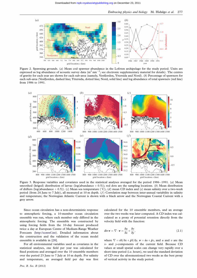
Figure 2. Spawning grounds. (a) Mean cod spawner abundance in the Lofoten archipelago for the study period. Units are

expressed as log abundance of acoustic survey data (m2 nm22; see electronic supplementary material for details). The centresof gravity for each year are shown for each sub-area (namely, Vestfjorden, Yttersida and Nord). (b) Percentage of spawners foreach sub-area (Vestfjorden, dashed line; Yttersida, dotted line; Nord, solid line) and log abundance of total spawners (red line)from 1986 to 1991.

800

(a) (b) (c)

(d) (e) ( f )

4

3

2

1

0.10 34.6

0.5

–0.5

0.0

34.4

34.2

34.0

33.8

33.6

33.4

33.2

0.08

0.06

0.04

0.02

1.5 10

9

8

7

5

5

4

1.0

0.5

–0.5

0

700

600

500

grid

loca

tion

y (k

m)

400

300

200

400 600 800 1000 1200 1400

800

700

600

500

grid

loca

tion

y (k

m)

grid location x (km)

400

300

200

800 900 1000 11001200 13001400 1500grid location x (km)

800 900 1000 11001200 13001400 1500grid location x (km)

800 900 1000 11001200 13001400 1500

800 900 1000 11001200 13001400 1500 800 900 1000 11001200 13001400 1500

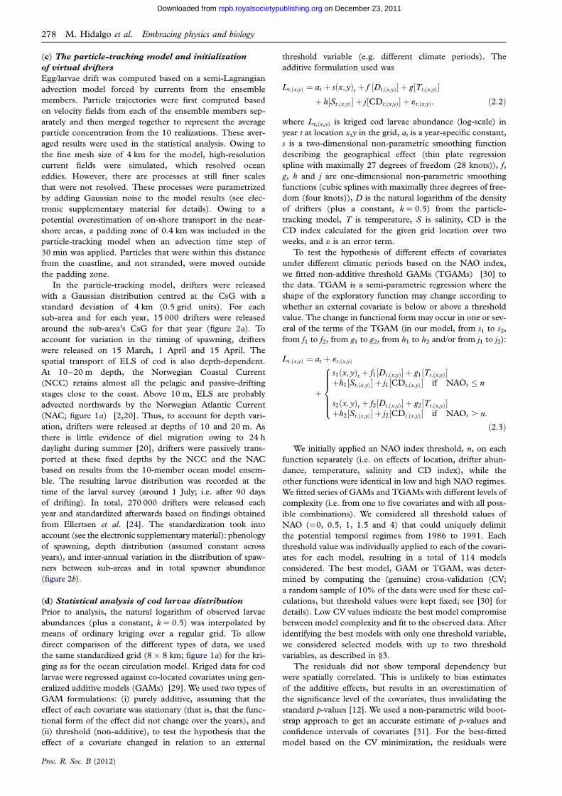
Figure 3. Response variables and covariates used in the statistical analyses averaged for the period 1986–1991. (a) Mean

smoothed (kriged) distribution of larvae (log(abundance þ 0.5)); red dots are the sampling locations. (b) Mean distributionof drifters (log(abundance þ 0.5)). (c) Mean sea temperature (8C), (d) mean CD index and (e) mean salinity over a two-weekperiod (from 24 June to 7 July), all measured at 10 m depth. ( f ) Correlation map between inter-annual variability in salinityand temperature; the Norwegian Atlantic Current is shown with a black arrow and the Norwegian Coastal Current with a

grey arrow.

Embracing physics and biology M. Hidalgo et al. 277

on December 23, 2011rspb.royalsocietypublishing.orgDownloaded from

Since ocean circulation has a non-deterministic response

to atmospheric forcing, a 10-member ocean circulation

ensemble was run, where each member only differed in the

atmospheric forcing. The ensemble was constructed by

using forcing fields from the 10-day forecast produced

twice a day at European Centre of Medium-Range Weather

Forecasts (http://ecmwf.int). Detailed information about

the construction and the validation of the ocean model

ensemble is available in [28].

For all environmental variables used as covariates in the

statistical analyses, one field per year was calculated for

fixed positions and averaged over the 10 ensemble members

over the period 23 June to 7 July at 10 m depth. For salinity

and temperature, an averaged field per day was first

Proc. R. Soc. B (2012)

calculated for the 10 ensemble members, and an average

over the two weeks was later computed. A CD index was cal-

culated as a proxy of potential retention directly from the

velocity field with the function:

divn ¼ r � n ¼ du

dxþ dv

dy; ð2:1Þ

where r ¼ id=dxþ jd=dy; n ¼ iuþ jv, and u and v are the

x- and y-components of the current field. Because CD

values at small spatial scales can change very rapidly over a

short time period (i.e. hours), we used the standard deviation

of CD over the aforementioned two weeks as the best proxy

of vertical activity in the study period.

278 M. Hidalgo et al. Embracing physics and biology

on December 23, 2011rspb.royalsocietypublishing.orgDownloaded from

(c) The particle-tracking model and initialization

of virtual drifters

Egg/larvae drift was computed based on a semi-Lagrangian

advection model forced by currents from the ensemble

members. Particle trajectories were first computed based

on velocity fields from each of the ensemble members sep-

arately and then merged together to represent the average

particle concentration from the 10 realizations. These aver-

aged results were used in the statistical analysis. Owing to

the fine mesh size of 4 km for the model, high-resolution

current fields were simulated, which resolved ocean

eddies. However, there are processes at still finer scales

that were not resolved. These processes were parametrized

by adding Gaussian noise to the model results (see elec-

tronic supplementary material for details). Owing to a

potential overestimation of on-shore transport in the near-

shore areas, a padding zone of 0.4 km was included in the

particle-tracking model when an advection time step of

30 min was applied. Particles that were within this distance

from the coastline, and not stranded, were moved outside

the padding zone.

In the particle-tracking model, drifters were released

with a Gaussian distribution centred at the CsG with a

standard deviation of 4 km (0.5 grid units). For each

sub-area and for each year, 15 000 drifters were released

around the sub-area’s CsG for that year (figure 2a). To

account for variation in the timing of spawning, drifters

were released on 15 March, 1 April and 15 April. The

spatial transport of ELS of cod is also depth-dependent.

At 10–20 m depth, the Norwegian Coastal Current

(NCC) retains almost all the pelagic and passive-drifting

stages close to the coast. Above 10 m, ELS are probably

advected northwards by the Norwegian Atlantic Current

(NAC; figure 1a) [2,20]. Thus, to account for depth vari-

ation, drifters were released at depths of 10 and 20 m. As

there is little evidence of diel migration owing to 24 h

daylight during summer [20], drifters were passively trans-

ported at these fixed depths by the NCC and the NAC

based on results from the 10-member ocean model ensem-

ble. The resulting larvae distribution was recorded at the

time of the larval survey (around 1 July; i.e. after 90 days

of drifting). In total, 270 000 drifters were released each

year and standardized afterwards based on findings obtained

from Ellertsen et al. [24]. The standardization took into

account (see the electronic supplementary material): phenology

of spawning, depth distribution (assumed constant across

years), and inter-annual variation in the distribution of spaw-

ners between sub-areas and in total spawner abundance

(figure 2b).

(d) Statistical analysis of cod larvae distribution

Prior to analysis, the natural logarithm of observed larvae

abundances (plus a constant, k ¼ 0.5) was interpolated by

means of ordinary kriging over a regular grid. To allow

direct comparison of the different types of data, we used

the same standardized grid (8 � 8 km; figure 1a) for the kri-

ging as for the ocean circulation model. Kriged data for cod

larvae were regressed against co-located covariates using gen-

eralized additive models (GAMs) [29]. We used two types of

GAM formulations: (i) purely additive, assuming that the

effect of each covariate was stationary (that is, that the func-

tional form of the effect did not change over the years), and

(ii) threshold (non-additive), to test the hypothesis that the

effect of a covariate changed in relation to an external

Proc. R. Soc. B (2012)

threshold variable (e.g. different climate periods). The

additive formulation used was

Lt;ðx;yÞ ¼ at þ sðx; yÞt þ f ½Dt;ðx;yÞ� þ g½Tt;ðx;yÞ�þ h½St;ðx;yÞ� þ j½CDt;ðx;yÞ� þ 1t;ðx;yÞ; ð2:2Þ

where Lt,(x,y) is kriged cod larvae abundance (log-scale) in

year t at location x,y in the grid, at is a year-specific constant,

s is a two-dimensional non-parametric smoothing function

describing the geographical effect (thin plate regression

spline with maximally 27 degrees of freedom (28 knots)), f,

g, h and j are one-dimensional non-parametric smoothing

functions (cubic splines with maximally three degrees of free-

dom (four knots)), D is the natural logarithm of the density

of drifters (plus a constant, k ¼ 0.5) from the particle-

tracking model, T is temperature, S is salinity, CD is the

CD index calculated for the given grid location over two

weeks, and 1 is an error term.

To test the hypothesis of different effects of covariates

under different climatic periods based on the NAO index,

we fitted non-additive threshold GAMs (TGAMs) [30] to

the data. TGAM is a semi-parametric regression where the

shape of the exploratory function may change according to

whether an external covariate is below or above a threshold

value. The change in functional form may occur in one or sev-

eral of the terms of the TGAM (in our model, from s1 to s2,

from f1 to f2, from g1 to g2, from h1 to h2 and/or from j1 to j2):

Lt;ðx;yÞ ¼ at þ 1t;ðx;yÞ

þ

s1ðx; yÞt þ f1½Dt;ðx;yÞ� þ g1½Tt;ðx;yÞ�þh1½St;ðx;yÞ� þ j1½CDt;ðx;yÞ� if NAOt � n

s2ðx; yÞt þ f2½Dt;ðx;yÞ� þ g2½Tt;ðx;yÞ�þh2½St;ðx;yÞ� þ j2½CDt;ðx;yÞ� if NAOt . n:

8>>>><>>>>:

ð2:3Þ

We initially applied an NAO index threshold, n, on each

function separately (i.e. on effects of location, drifter abun-

dance, temperature, salinity and CD index), while the

other functions were identical in low and high NAO regimes.

We fitted series of GAMs and TGAMs with different levels of

complexity (i.e. from one to five covariates and with all poss-

ible combinations). We considered all threshold values of

NAO (¼0, 0.5, 1, 1.5 and 4) that could uniquely delimit

the potential temporal regimes from 1986 to 1991. Each

threshold value was individually applied to each of the covari-

ates for each model, resulting in a total of 114 models

considered. The best model, GAM or TGAM, was deter-

mined by computing the (genuine) cross-validation (CV;

a random sample of 10% of the data were used for these cal-

culations, but threshold values were kept fixed; see [30] for

details). Low CV values indicate the best model compromise

between model complexity and fit to the observed data. After

identifying the best models with only one threshold variable,

we considered selected models with up to two threshold

variables, as described in §3.

The residuals did not show temporal dependency but

were spatially correlated. This is unlikely to bias estimates

of the additive effects, but results in an overestimation of

the significance level of the covariates, thus invalidating the

standard p-values [12]. We used a non-parametric wild boot-

strap approach to get an accurate estimate of p-values and

confidence intervals of covariates [31]. For the best-fitted

model based on the CV minimization, the residuals were

Embracing physics and biology M. Hidalgo et al. 279

on December 23, 2011rspb.royalsocietypublishing.orgDownloaded from

extracted, rescaled to the same variance as the estimated

scale parameter of the model and randomly replaced

among years (sampling with replacement), before being

used as response variable in the model (having the same set

of covariates as the original model; see details in [32]). As

an additional test of the significance of the threshold effects,

we used an alternative CV approach, in which we left out data

for whole years at a time (instead of a random 10% of the

data). We then confirmed that the final selected threshold

model (but without a year-specific intercept) had higher

predictive power for data cases (years) not used when fitting

the model compared with alternative formulations without

thresholds.

3. RESULTS(a) Spawning aggregations

Both the spatial distribution (CsG) and abundance within

sub-areas varied among years (figure 2a,b; see spawner

distribution and CsG for all the years in the electronic

supplementary material, figure S1). The CsG were gener-

ally more offshore from 1987 to 1989 compared with

1986, 1990 and 1991 in Yttersida and Nord. Addition-

ally, CsG were in the outer area of Vestfjorden from

1987 to 1989 and 1991. Pairwise correlations among

CsG showed inter-annual consistency in the spatial vari-

ation: x-axis positions (note spatial coordinates refer to

the oceanographic model domain; see figure 1a) were

highly and positively correlated between Vestfjorden and

Yttersida (Spearman, r ¼ 0.92, p , 0.05), while y-axis

positions were negatively correlated between Nord and

Vestfjorden (r ¼ 20.74, p , 0.05). With the exception

of 1987 and 1991, the relative contribution of each sub-

area to total annual cod abundance in Lofoten was quite

constant (figure 2b). In 1987, 51 per cent of the fish spawned

in the Nord sub-area, compared with 15 to 25 per cent for

most years. In 1991, the year with highest total spawner

abundance, only 6 per cent spawned in this sub-area.

(b) Particle-tracking model

Maps of simulated larvae distributions after 90 days of drift-

ing from the mean date of spawning (1 April) and from each

sub-area show only the predicted effects of inter-annual

variation in the current pattern (see electronic supplemen-

tary material, figure S2). By taking into account variation

in the relative contribution of each sub-area, the model pre-

dicted extensive spreading of drifters in the Barents Sea for

1987 (see electronic supplementary material, figure S3a).

After taking into account variation in total spawner abun-

dance, extensive spreading was also predicted for 1991

(electronic supplementary material, figure S3b). Higher

abundance of drifters in the near-shore areas is a general

pattern in the distributions obtained.

(c) Spatial analyses

We analysed the distribution of larvae estimated from

survey data (figure 3a; see all the years in the electronic

supplementary material, figure S4, and its inter-annual

variation in electronic supplementary material, figure S5)

using additive or non-additive models with one to five co-

variates. Besides drifter density estimates described above

(figure 3b; all years are shown in the electronic supplemen-

tary material, figure S3b), temperature, salinity and CD

index were used as covariates (figures 3c–e; all years are

Proc. R. Soc. B (2012)

shown in the electronic supplementary material, figure

S6). Results show that models with non-additive threshold

effects (TGAM) were more parsimonious (as given by CV

values) compared with purelyadditive models (see electronic

supplementary material, table S1). The most parsimonious

TGAMs generally identified a threshold of NAO ¼ 1, corre-

sponding to two short-term climatic periods: 1986–1988

(NAO , 1, ‘cold’ period) and 1989–1991 (NAO . 1,

‘warm’ period). The preliminary best models included all

five covariates and an NAO ¼ 1 threshold on either:

(i) spatial location, the best model (see electronic sup-

plementary material, table S1, model 80); (ii) temperature,

the second best model (see electronic supplementary

material, table S1, model 76); or (iii) drifter abundance,

the third best model (see electronic supplementary material,

table S1, model 78). These models were sequentially com-

bined, applying an NAO ¼ 1 threshold on two or three

covariates, and resulted in three models (models 81–83).

Two of these models included salinity, although salinity

was not significant (p ¼ 0.18) when applying a non-para-

metric bootstrap on model 81. Spatial heterogeneity in the

correlation between salinity and temperature as shown in

our study (figure 3f ) justifies the inclusion of both tempera-

ture and salinity in our models. The final model (see

electronic supplementary material, table S1, model 83;

figure 4) explained 84 per cent of the observed variance in

larvae abundance.

The final model is shown in figure 4. The partial effect of

year (p , 0.05; figure 4a) shows an increasing trend, partly

coinciding with the trend in spawner abundance (figure 1b).

The relationship between drifter abundance and observed

larval abundance is asymptotic (p , 0.05; figure 4b). Temp-

erature effects differed between the climatic periods (1986–

1988 and 1989–1991; the two effects p , 0.05; figure 4c).

Specifically, during the warm period, high abundances of

larvae were found in waters with temperatures around

9.58C, while in the cold period the effect of temperature

was stronger and the highest abundances were found in

temperatures above 108C. The effect of the geographical

location showed a clear and significant difference between

periods, suggesting positive anomalies in the southwestern

parts of the study area in the period 1986–1988 (p ,

0.05; figure 4d) and in the northeastern parts in the

period 1989–1991 (p , 0.05; figure 4e). Note that these

effects remain while accounting for local environmental co-

variates. Finally, there was some evidence for an effect of

CD activity (p¼ 0.073; figure 4f ). To assess the unique

contribution of each covariate, we calculated the difference

in percentage of variance explained between the full model

and a model with the given term removed. The spatial term

and the partial effect of year contributed the most (25 and

19 per cent, respectively), while temperature, drifter abun-

dance and CD activity explained 11.8, 7.2 and 1.8 per

cent, respectively.

4. DISCUSSIONOur study reveals how the abundance and distribution of

spawners, ocean circulation and hydrographical environ-

mental conditions in combination modify the spatial

distribution of ELS, and how the effects of these factors

differ between two periods with contrasting states of the

NAO. The best model obtained explains a major fraction

of the observed variance and includes drifter abundance

4(a)

(d) (e) ( f )

(b) (c)

3

2

1

4

3

2

1

0

–1

–2

–3

0

86

800

700

600

500

400

300

200800 900 1000 1100

grid location x (km)

grid

loca

tion

y (k

m)

800 2.0

1.5

1.0

0.5

–0.5

–1.0

0.0

700

600

500

400

300

200

grid

loca

tion

y (k

m)

1200 1300 14001500 800 900 1000 1100

grid location x (km)

1200 1300 1400 1500 0 0.02 0.04

convergence/divergence index

0.06 0.08 0.10

87

0.60.8

0.20.4

–0.4–0.2

–0.6

–0.2 0.20

0.2

–0.2

0.8 –0.8

–0.6

–0.2

0

1

0.6

–0.4

0.4

0.4

–0.4

–1

–0.8

–0.8

1

1

0

88 89year

90 91 –0.5 0 0.5 1.0drifters (ln [N/grid unit])

1.5 2.0 2.5

part

ial e

ffec

t of

fact

or

addi

tive

effe

ct

4

3

2

1

0

–1

–2

–3

5 6 7 8 9temperature (°C)

10 11 12

addi

tive

effe

ctad

ditiv

e ef

fect

–1

–2

Figure 4. Results of the best model using non-additive threshold effects: (a) partial effect of year factor, (b) drifter effect,(c) temperature effect for low and high NAO regimes (represented in blue and red, respectively), (d) partial spatial effectfor low NAO regime (less than 1, 1986–1988), (e) partial spatial effect for high NAO regime (greater than 1, 1989–1991)and ( f ) CD index effect. Whole and broken lines indicate fitted partial effects with two times standard deviation estimatedfrom bootstrapping, respectively. Confidence intervals for the spatial effects are shown in figure S7 in the electronic supplemen-

tary material. Points for (b), (c) and (f) represent the partial residuals for each smoothed term. Note that the scale of the y-axisfor CD index is different from (a–c).

280 M. Hidalgo et al. Embracing physics and biology

on December 23, 2011rspb.royalsocietypublishing.orgDownloaded from

(which integrates effects of spawner abundance and dis-

tribution, and larval advection) and the CD index as

additive covariates, and temperature and geographical

location as non-additive covariates—their effects changing

between a high and low NAO index. We show that by com-

bining ocean circulation models and statistical techniques,

we can reproduce the spatio-temporal dynamics of NEA

cod larvae, and reveal the environmental factors shaping

their distribution. Thus, this study provides a novel and

promising methodological framework for integrating quan-

titative information on spawner aggregations with ocean

circulation and hydrography in statistical spatial analyses

of pelagic ELS.

(a) Implications of spawner distribution for

advection and survival

The starting position of drifters fundamentally controls

the directions and distance of their drift paths. Therefore,

the spatio-temporal distribution of spawners (when,

where and how many) is crucial for proper initialization

of particle-tracking models [8]. Although cod spawning

phenology and geographical location is a fine-tuned evol-

utionary strategy developed through generations to

maximize survival [33], large-scale inter-decadal displace-

ments of spawning aggregations have been described and

attributed to both climate [34] and fishing effects on size

structure [35]. From the mid-1980s, a warm period

during which cod populations were demographically

eroded, the Lofoten grounds were the most important

area for the spawner aggregations. Our results add to

this picture by emphasizing the effects of small-scale vari-

ation within the Lofoten archipelago. The inter-annual

variation in the CsG was consistent among sub-areas,

Proc. R. Soc. B (2012)

indicating a certain spatial synchrony in spawning aggre-

gation patterns. However, we cannot establish whether

the temporal variation of the fine-scale structure in the

spawning areas was related to climate, mating behaviour

or changes in the population density over time.

Our results confirm that spatio-temporal variation in

spawner aggregations within and among sub-areas

around Lofoten combined with varying circulation pat-

terns impact the resultant spatial distribution of eggs

and larvae. In 1987, for example, the higher contribution

of spawners at Nord (the more offshore sub-area)

facilitated a more extensive spreading of ELS. Such

spreading may ensure that a sufficient number of eggs

and larvae encounter environmentally favourable con-

ditions ([36] and references therein), and thus may have

contributed to the higher larval survival found that year

(figure 4a). High survival in 1991, when high spawner

abundance caused extensive spreading of drifters into

the Barents Sea, is consistent with this explanation.

(b) Spatial distribution of early life stages of cod

The asymptotic relationship observed between drifter

abundance and observed larval abundance could be

related to lower survival of ELS very close to the coast,

which is where the highest concentrations of drifters

occurred. Stranding of eggs onto the coast, higher preda-

tion during the drifting process and higher mortality at

high larval densities (e.g. because of food limitation) are

all factors that may have contributed to low survival.

However, it is worth noting that the unresolved currents

in the coastal areas owing to the confluence of multiple

drivers interacting at fine to meso scales near shore

could potentially overestimate drifters along the coast

Embracing physics and biology M. Hidalgo et al. 281

on December 23, 2011rspb.royalsocietypublishing.orgDownloaded from

[6]. Although a padding zone was included in the

particle-tracking model to mitigate this problem, overesti-

mation of drifter density along the coast is certainly

possible. Nevertheless, the spatial pattern of our results

is consistent with other studies applying different ocean

models [2,20].

Having accounted for drifter abundance (i.e. the com-

bined effect of spawner distribution and larval advection),

the statistical model captures the potential effect of the

other covariates on larval distribution. The most novel

and striking result is the different contribution of

temperature and spatial location under two short-term

periods with contrasting climate conditions (1986–1988

and 1989–1991). Previous studies have shown that both

temperature and recruitment success of cod in the study

area are higher during NAO-positive years [36]. Our

analysis adds to this picture by showing that the generally

positive temperature–larval abundance relation was

weaker in years with high NAO values. During the gener-

ally warm (NAO-positive) 1989–1991 period, high

abundances of larvae were found in water masses with a

relatively wide range of temperatures. During the colder

1986–1988 period, high larval abundances were only

found in the warmest waters. The causal basis for this

difference is not clear, but we note that temperature is

positively associated with food availability and that there

is a better temporal match between the development of

cod larvae and their zooplankton prey in warm years

[24,37]. We speculate that in cold periods, zooplankton

of appropriate size is only available in sufficient quantity

in the warmest water masses, whereas in warm periods,

zooplankton conditions are favourable over larger areas

(and a wider temperature range). This is supported by

recent evidence showing that zooplankton biomass pre-

dicts survival of ELS of NEA cod [25], and how

prolonged temporal overlap between fish larvae and

their prey in warm years enhances cumulative growth

and survival [37].

Lastly, the partial effect of geographical location of

larvae shows a clear and significant difference between

the two periods. Based on earlier work, the southwestern

distribution of larvae could potentially be explained by

a reduction in transport during cold periods (NAO-nega-

tive years) [2,17]. However, as far as the drifters capture

the current transport, the spatial pattern summarizes

the variability left over by the selected environmental co-

variates, and therefore could indicate that the spatial

pattern in mortality differs between the two periods. Sev-

eral factors could cause such a shift in mortality, such as

changes in the distribution of predators or prey. Higher

zooplankton biomass in NAO-positive years has indeed

been shown for the ‘downstream’ [38] but not the

‘upstream’ (L. C. Stige 2011, unpublished data) part of

our study area, consistent with such a role of prey.

A potential role of predators is supported by the results

of Ciannelli et al. [18] suggesting that cannibalism may

modify the distribution pattern of 1-year-old cod in the

Barents Sea. On the other hand, the climatic influence

on the transport cannot be disregarded. For example,

during windy conditions (more frequent in NAO-positive

years) eggs are mixed deeper in the water column, where

NCC favours a more downstream distribution [20].

Further, our results also showed that CD activity could

affect the observed larval distribution. The highest CD

Proc. R. Soc. B (2012)

is found in the southern part of the shallow Barents

Sea, where the NAC is deflected northwards and the

NCC spreads out from the coast (figure 1a). This process

contributes to a front developing between the water

masses, creating a convergence zone with increased con-

centration of phytoplankton and zooplankton [39].

Finally, CD activity in this area could slow down the

northward transport of larvae and reinforce the southern

distribution observed in cold periods.

(c) Implications and future challenges for an

integrative approach

Disentangling the drivers of larval dispersal and the

consequences for the spatio-temporal patterns of ELS

distribution is an inherently biophysical problem. This

requires an interdisciplinary effort, integrating tools from

different scientific disciplines. This study provides a new

biophysical framework to link observational information

from spawner distributions to larval distributions, taking

into account variability in ocean circulation and the

hydrographical environmental conditions of the larval

habitat. Although we provide some methodological

advances, such as the use of a model ensemble to include

uncertainty into the numerically modelled larval

distributions and covariates, there is also room for

improvement. Key challenges for future studies include

improvement in the near-shore oceanographic modelling,

accounting for the size structure of the mature stock,

inclusion of larval behaviour linked to observations (e.g.

vertical migration linked to observations of food avail-

ability) and accounting for the lack of synopticity in the

ELS surveys.

5. CONCLUSIONSAlthough the circulation pattern is the main physical

factor shaping the spatial distribution of larvae, climate

indirectly modifies this distribution by affecting larval sur-

vival (e.g. [25,37]). It is worth noticing that inter-annual

variation in spatial distribution of spawners at scales of

less than 100 km can affect the spread of larvae into the

larval habitat. In essence, our study highlights that

larvae were distributed over a wider temperature range,

over a larger area and more downstream in warm periods

owing to a combination of (i) higher abundance of spaw-

ners, (ii) an increase of ocean transport, (iii) higher overall

survival (possibly because of better food availability and/

or escape from predation), and (iv) a likely change in

the spatial pattern in natural survival, hypothetically

caused by changes in spatial distribution of predators or

prey. ELS of many marine fish species experience differ-

ent environmental conditions throughout their

distribution ranges. The combination of hydrodynamical

and statistical modelling is a promising tool for integrat-

ing information about oceanographic processes, small-

scale ecological mechanisms and large-scale observations

to draw statistically robust inferences about the processes

shaping ELS distribution and survival. Our study shows

that such a tool is likely to provide novel knowledge,

even for highly well-studied species and systems.

M.H., Y.G., D.H., G.O. and L.C.S. received support fromthe Research Council of Norway (projects no. 173487 and178434). M.H. thanks M. Llope for the advice anddiscussions on an early version of this manuscript and for

282 M. Hidalgo et al. Embracing physics and biology

on December 23, 2011rspb.royalsocietypublishing.orgDownloaded from

help in the data analysis, Lee Hsiang Liow and JasonD. Whittington for reviewing an advanced version, and twoanonymous reviewers for their helpful comments.

REFERENCES1 Cowen, R. K. & Sponaugle, S. 2009 Larval dispersal

and marine population connectivity. Annu. Rev. Mar.Sci. 1, 443–466. (doi:10.1146/annurev.marine.010908.163757)

2 Vikebø, F., Jørgensen, C., Kristiansen, T. & Fiksen, Ø.2007 Drift, growth, and survival of larval NortheastArctic cod with simple rules of behaviour. Mar. Ecol.Prog. Ser. 347, 207–219. (doi:10.3354/meps06979)

3 O’Connor, M. I., Bruno, J. F., Gaines, S. D., Halpern, B.S., Lester, S. E., Kinlan, B. P. & Weiss, J. M. 2007 Temp-erature control of larval dispersal and the implication for

marine ecology, evolution and conservation. Proc. NatlAcad. Sci. USA 104, 1266–1271. (doi:10.1073/pnas.0603422104)

4 Rindorf, A. & Lewy, P. 2006 Warm, windy winters drivecod north and homing of spawners keeps them there.

J. Appl. Ecol. 43, 445–453. (doi:10.1111/j.1365-2664.2006.01161.x)

5 Lett, C., Rose, K. A. & Megrey, B. A. 2010 Biophysicalmodels. In Climate change and small pelagic fish (edsD. Checkley, J. Alheit, Y. Oozeki & C. Roy), pp.

88–111. Cambridge, UK: Cambridge University Press.6 Werner, F. E., Cowen, R. K. & Paris, C. B. 2007 Coupled

biological and physical models: present capabilities andnecessary developments for future studies of populationsconnectivity. Oceanography 20, 54–69.

7 Fiksen, Ø., Jørgensen, C., Kristiansen, T., Vikebø, F. &Huse, G. 2007 Linking behavioural ecology and ocean-ography: larval behaviour determines growth, mortalityand dispersal. Mar. Ecol. Prog. Ser. 347, 195–205.

(doi:10.3354/meps06978)8 Gallego, A. & North, E. W. 2009 Biological processes. In

Manual of recommended practices for modelling physical–biological interactions during the fish early life (eds E. W.North, A. Gallego & P. Peptigas), pp. 20–59. ICES

Cooperative Research Report no. 295. Copenhagen,Denmark: ICES.

9 Boyce, D. G., Lewis, M. R. & Worm, B. 2010 Globalphytoplankton decline over the past century. Nature466, 591–596. (doi:10.1038/nature09268)

10 Fox, C. J., O’Brien, C. M., Dickey-Collas, M. & Nash,R. D. M. 2000 Patterns in the spawning of cod (Gadusmorhua L.), sole (Solea solea L.) and plaice (Pleuronectesplatessa L.) in the Irish Sea as determined by generalisedadditive modelling. Fish Oceanogr. 9, 33–49. (doi:10.

1046/j.1365-2419.2000.00120.x)11 Bacheler, N. M., Ciannelli, L., Bailey, K. M. & Duffy-

Anderson, J. T. 2010 Spatial and temporal patterns ofwalleye pollock (Theragra chalcogramma) spawning inthe eastern Bering Sea inferred from egg and larval dis-

tributions. Fish. Oceanogr. 19, 107–120. (doi:10.1111/j.1365-2419.2009.00531.x)

12 Ciannelli, L., Fauchald, P., Chan, K. S., Agostini, V. N. &Dingsør, G. E. 2008 Spatial fisheries ecology: recent pro-

gress and future prospects. J. Mar. Syst. 71, 223–236.(doi:10.1016/j.jmarsys.2007.02.031)

13 North, E. W., Schlag, Z., Hood, R. R., Li, M., Zhong,L., Gross, T. & Kennedy, V. S. 2008 Vertical swimmingbehavior influences the dispersal of simulated oyster

larvae in a coupled article-tracking and hydrodynamicmodel of Chesapeake Bay. Mar. Ecol. Prog. Ser. 359,99–115. (doi:10.3354/meps07317)

14 Brickman, D., Marteinsdottir, G. & Taylor, L. 2007 For-mulation and application of an efficient optimized

Proc. R. Soc. B (2012)

biophysical model. Mar. Ecol. Prog. Ser. 347, 275–284.(doi:10.3354/meps06984)

15 Hinrichsen, H. H., Mollmann, C., Voss, R., Koster, F. W. &

Kornilovs, G. 2002 Biophysical modelling of larval Balticcod (Gadus morhua L.) growth and survival. Can. J. FishAquat. Sci. 59, 1858–1873. (doi:10.1139/f02-149)

16 Baumann, H., Hinrichsen, H. H., Mollmann, C., Koster,F. W., Malzahn, A. M. & Temming, A. 2006 Recruitment

variability in Baltic sprat, Sprattus sprattus, is tightlycoupled to temperature and transport patterns affectingthe larval and early juvenile stages. Can. J. Fish Aquat.Sci. 63, 2191–2201. (doi:10.1139/f06-112)

17 Ottersen, G., Helle, K. & Bogstad, B. 2002 Do abioticmechanisms determine interannual variability in length-at-age of juvenile Arcto-Norwegian cod? Can. J. FishAquat. Sci. 59, 57–65. (doi:10.1139/f01-197)

18 Ciannelli, L., Dingsør, G. E., Bogstad, B., Ottersen, G.,

Chan, K. S., Gjøsæter, H., Stiansen, J. E. & Stenseth,N. C. 2007 Spatial anatomy of species survival: effects ofpredation and climate-driven environmental variability.Ecology 88, 635–646. (doi:10.1890/05-2035)

19 Dingsør, G. E., Ciannelli, L., Chan, K. S., Ottersen, G. &

Stenseth, N. S. 2007 Density dependence and density inde-pendence during the early life stages of four marine fishstocks. Ecology 88, 625–634. (doi:10.1890/05-1782)

20 Vikebø, F., Sundby, S., Adlandsvik, B. & Fiksen, Ø. 2005The combined effect of transport and temperature on

distribution and growth of larvae and pelagic juvenilesof Arcto-Norwegian cod. ICES J. Mar. Sci. 62,1375–1386. (doi:10.1016/j.icesjms.2005.05.017)

21 Kristiansen, T., Vikebø, F., Sundby, S., Huse, G. &

Fiksen, Ø. 2009 Modeling growth of larval cod (Gadusmorhua) in large-scale seasonal and latitudinal environ-mental gradients. Deep-Sea Res. II 56, 2001–2011.(doi:10.1016/j.dsr2.2008.11.011)

22 Hurrell, J. W. 1995 Decadal trends in the North Atlantic

Oscillation: regional temperatures and precipitation. Science169, 676–679. (doi:10.1126/science.269.5224.676)

23 Helle, K. & Pennington, M. 1999 The relation of the spatialdistribution of early juvenile cod (Gadus morhua L.) in theBarents Sea to zooplankton density and water flux during

the period 1978–1984. ICES J. Mar. Sci. 56, 15–27.(doi:10.1006/jmsc.1998.0427)

24 Ellertsen, B., Fossum, P., Solemdal, P. & Sundby, S.1989 Relation between temperature and survival ofeggs and first feeding larvae of northeast Arctic cod

(Gadus morhua L.). Rapports et Proces-verbaux desReunions Conseil International pour l’Exploration de la Mer191, 209–219.

25 Stige, L. C., Ottersen, G., Dalpadado, P., Chan, K.-S.,

Hjermann, D. Ø., Lajus, D. L., Yaragina, N. A. &Stenseth, N. C. 2010 Direct and indirect climate forcingin a multi-species marine system. Proc. R. Soc. B 277,3411–3420. (doi:10.1098/rspb.2010.0602)

26 Engedahl, H., Lunde, A., Melsom, A. & Shi, X. B. 2001

New schemes for vertical mixing in MI-POM and MICOM.Research report no. 118. Oslo, Norway: NorwegianMeteorological Institute.

27 Røed, L. & Debernard, J. 2004 Description of an integratedflux and sea-ice model suitable for coupling to an ocean andatmosphere model. Met. no. report 4/2004. Oslo, Norway:Norwegian Meteorological Institute.

28 Melsom, A. & Fossum, I. 2009 Validation of an oceanmodel ensemble for the Barents Sea and the northeasternNordic Seas. Met. no. Report 2/2009. Oslo, Norway:

Norwegian Meteorological Institute.29 Hastie, T. J. & Tibshirani, R. J. 1990 Generalized additive

models. London, UK: Chapman and Hall.30 Ciannelli, L., Chan, K. S., Bailey, K. M. & Stenseth,

N. C. 2004 Nonadditive effects of the environment on

Embracing physics and biology M. Hidalgo et al. 283

on December 23, 2011rspb.royalsocietypublishing.orgDownloaded from

the survival of a large marine fish population. Ecology 85,3418–3427. (doi:10.1890/03-0755)

31 Mammen, E. 1993 Bootstrap and wild bootstrap for high

dimensional linear models in resampling. Ann. Stat. 21,255–285. (doi:10.1214/aos/1176349025)

32 Stige, L. C., Ottersen, G., Brander, K., Chan, K.-S. &Stenseth, N. C. 2006 Cod and climate: effect of theNorth Atlantic Oscillation on recruitment in the North

Atlantic. Mar. Ecol. Prog. Ser. 325, 227–241. (doi:10.3354/meps325227)

33 Jørgensen, C., Dunlop, E. S., Opdal, A. F. & Fiksen, Ø.2008 The evolution of spawning migrations: state depen-

dence and fishing-induced changes. Ecology 89, 3436–3448. (doi:10.1890/07-1469.1)

34 Sundby, S. & Nakken, O. 2008 Spatial shifts in spawninghabitats of Arcto-Norwegian cod related to multidecadalclimate oscillations and climate change. ICES J. Mar. Sci.65, 953–962. (doi:10.1093/icesjms/fsn085)

35 Opdal, A. F. 2010 Fisheries change spawning ground dis-tribution of northeast Arctic cod. Biol. Lett. 6, 261–264.(doi:10.1098/rsbl.2009.0789)

Proc. R. Soc. B (2012)

36 Ottersen, G., Hjermann, D. O. & Stenseth, N. C.2006 Changes in spawning stock structure strengthenthe link between climate and recruitment in a

heavily fished cod (Gadus morhua) stock. FishOceanogr. 15, 230–243. (doi:10.1111/j.1365-2419.2006.00404.x)

37 Kristiansen, T., Drinkwater, K. F., Lough, R. G. &Sundby, S. 2011 Recruitment variability in North

Atlantic cod and match-mismatch dynamics. PLoSONE 6, e17456. (doi:10.1371/journal.pone.0017456)

38 Stige, L. C., Lajus, D. L., Chan, K. S., Dalpadado, P.,Basedow, S. L., Berchenko, I. & Stenseth, N. C. 2009

Climatic forcing of zooplankton dynamics is strongerduring low densities of planktivorous fish. Limnol.Oceanogr. 54, 1025–1036. (doi:10.4319/lo.2009.54.4.1025)

39 Skarðhamar, J., Slagstad, D. & Edvardsen, A. 2007

Plankton distributions related to hydrography andcirculation dynamics on a narrow continental shelf offNorthern Norway. Estuarine Coastal Shelf Sci. 75,381–392. (doi:10.1016/j.ecss.2007.05.044)