Science of the Total Environment 444 (2013) 128–137

Contents lists available at SciVerse ScienceDirect

Science of the Total Environment

j ourna l homepage: www.e lsev ie r .com/ locate /sc i totenv

Heavy metals, trace elements and sediment geochemistry at four Mediterraneanfish farms

I. Kalantzi a, T.M. Shimmield b, S.A. Pergantis c, N. Papageorgiou a, K.D. Black b, I. Karakassis a,⁎a Biology Department, University of Crete, Voutes University Campus, 71003, Heraklion, Crete, Greeceb Scottish Association for Marine Science, Scottish Marine Institute, Oban PA34 1QA, Scotland, United Kingdomc Chemistry Department, University of Crete, Voutes University Campus, 71003, Heraklion, Crete, Greece

H I G H L I G H T S

► Trace elements levels in sediments were studied in 4 Mediterranean fish farms.► Sediment grain size, organic content and redox affect element behavior.► For all elements, impacted anoxic sediments had higher levels than reference sites.► Some elements in oxic sediments had lower levels at impacted than reference sites.► Cu, Zn, Fe can affect aquatic life in anoxic-fine sediments, As in all sediment types.

⁎ Corresponding author. Tel.: +30 2810 394061; fax:E-mail address: karakassis@biology.uoc.gr (I. Karaka

0048-9697/$ – see front matter © 2012 Elsevier B.V. Allhttp://dx.doi.org/10.1016/j.scitotenv.2012.11.082

a b s t r a c t

a r t i c l e i n f o

Article history:Received 14 June 2012Received in revised form 19 November 2012Accepted 24 November 2012Available online xxxx

Keywords:Fish farmSedimentGeochemistryTrace elementheavy metals

Trace element concentrations in sediment were investigated at four fish farms in the Eastern MediterraneanSea. Fish farms effects were negligible beyond 25–50 m from the edge of the cages. Based on elemental dis-tribution, sediments from the farms were separated into coarse oxidized and silty reduced ones. Fish feed isricher in P, Zn and Cd than reference and impacted stations. Comparison among impacted stations and therespective reference stations shows that, in anoxic sediments, all elements had higher concentrations atthe impacted stations than at reference stations while in oxic sediments, many elemental concentrationswere lower at impacted stations than at reference stations. The behavior of elements and therefore their dis-tribution is affected by changes in sediment grain size, organic content and redox regime. Elements in sedi-ments around fish farms can be clustered into five groups according to these environmental variables. In siltyand anoxic sediments, element concentrations were higher than in coarse and oxic ones. Several approacheswere used to assess potential sediment toxicity (enrichment factors, geoaccumulation indices, contaminationfactors) as well as to assess the potential danger to aquatic life (Sediment Quality Guidelines, SQG). Cu, Znand Fe can cause from threshold to extreme effects on aquatic life in anoxic, fine-grained sediments and Ascan cause threshold effects in all types of sediment around fish farms. Other elements (Cr, Pb, Mn) can alsocause unwanted effects when compounded with elevated background levels.

© 2012 Elsevier B.V. All rights reserved.

1. Introduction

The distribution and fate of elements in marine sediments re-ceived considerable attention in the 1970s following the Minamataincident and, as a result, comprehensive protection of public healthfrom the most toxic heavy metals and elements in seafood wasachieved (McIntyre, 1995). It is known that changes in the redoxregime, free sulphide and organic matter affect the behavior of vari-ous metals and element species (Belias et al., 2003; Sutherland etal., 2007; Brooks and Mahnken, 2003; Russell et al., 2011; Jaysankaret al., 2009; Sarkar et al., 2004; Smith et al., 2005; Chou et al., 2002;

+30 2810 394408.ssis).

rights reserved.

Peltola et al., 2011). Such changes are known to occur in the prolifer-ating dead zones where the seabed is anoxic (Diaz and Rosenberg,2008).

Sediments consist of inorganic and organic particles with complexphysical, chemical and biological characteristics (Sarkar et al., 2004).They can scavenge some elements, thus acting as an adsorptive sinkwith metal concentrations many times greater than in the watercolumn. Sediments are therefore an appropriate matrix in which tomonitor contamination (Sarkar et al., 2004; Giarratano and Amin,2010; Cukrov et al., 2011; Carbonell et al., 1998). However, sedimentsare not only a sink but also a possible delayed source of these contam-inants into the water column due to desorption, remobilizationprocesses, redox reactions and degradation of sorptive substances(Cukrov et al., 2011; Sarkar et al., 2004; Christophoridis et al.,2009). Therefore metal contamination of surficial sediments could

129I. Kalantzi et al. / Science of the Total Environment 444 (2013) 128–137

directly affect seawater quality (Mendiguchía et al., 2006) and consti-tute a long-term source of contamination to the food web (Burton,2002; Cukrov et al., 2011).

Three-quarters of wild fish stocks are fully fished, overfished ordepleted according to the Food and Agriculture Organization (FAO)(Giarratano and Amin, 2010). Aquaculture currently provides a con-siderable proportion of edible fish which is expected to increase in fu-ture decades in order to meet the needs of the growing humanpopulation (Duarte et al., 2009). Fish farm wastes (uneaten feed,faeces, metabolic excretion products and effluent chemical speciessuch as medicines) can accumulate on sediments below or near thefish cages. This organic material represents a potential risk of contam-ination to the wider environment, exhibiting a variety of biological,chemical and ecological effects (Schendel et al., 2004; Salazar andSaldana, 2007). Much of the environmental impact of fish farms islocal (Kalantzi and Karakassis, 2006), but fish farms can generatelong-lived, persistent contaminants that may have (far-field) longrange environmental effects. In this case metals and trace elementscan be used as tracers to estimate the (far-field) long range influenceof aquaculture (Smith et al., 2005). Even though the accumulation ofheavy metals and trace elements in sediments below aquaculturecages has been identified to have a significant impact on benthic com-munities (Salazar and Saldana, 2007) it has received relatively littleattention (Dean et al., 2007; Jaysankar et al., 2009).

TheMediterranean is one of themost oligotrophicmarinewater bod-ies in theworld. This is reflected in the low carbon/high redox conditionsprevailing in marine sediments (Karakassis and Eleftheriou, 1997). Fishfarming sites occasionally represent “hypoxic or anoxic islands” in thishighly oligotrophic continuum which are likely to induce changes inmetal and element behavior and their interactions with the local marineorganisms. In theMediterranean, there has been limited study on the ef-fects of heavy metals and trace element enrichment of sediments underfish cages, with research thus far focusedmainly on Cu, Zn, Pb, Cd and Fe(Belias et al., 2003; Basaran et al., 2010; Pergent et al., 1999).

The objective of this study was to use state-of-the-art analytical tech-niques to determine the concentration of a wide range of metals andtrace elements in a large number of samples originating from severalfish farms with different background conditions. Simultaneously the de-termination of relevant geochemical variables was carried out in order toinvestigate the factors that control elemental distributions in sediments.

2. Materials and methods

2.1. Study areas

Sediment samples were collected at four seabass (Dicentrarchuslabrax) and gilthead seabream (Sparus auratus) farms in Greece — twolocated in the Aegean Sea (AEG1 and AEG2) and two in the Ionian Sea(ION1 and ION2). The sampling areas were selected from a largergroup of fish farms in an effort tomaximize variance in terms of physical(water temperature, water content, depth, sediment particle size) andgeochemical characteristics (redox, sulphide, chl-a, organic matter) inthe data set (Table 1). Sampled farms are anonymous as a condition ofco-operationwith the farmers. AEG1 and ION1 are located in shallow ex-posed straits ca 200–300 m from the shore. AEG2 lies in a semi-exposedarea and ION2 is located in a shallow and semi-enclosed bay. The sedi-ment around the farms of AEG1, AEG2 and ION1 is coveredwith seagrassP. oceanica dominated habitat except for a bare zone extending 5–80 mfrom the edge of the cages where the seagrass meadows were degradedor absent. Sampling was performed during the periods of July 2006(AEG2), July 2007 (ION1 and ION2) and February 2007 (AEG1).

2.2. Field sampling

Three replicates of sediment core samples (4.5 cm internal diameter)were collected by scuba divers under the cages (0 m distance from the

cage) as well as at 5, 10, 25 and 50 m from the edge of the cages down-stream in the residual current direction. Reference stations with similardepth and substratum type but not affected by farm wastes wereestablished 400–1000 m fromeach farm. The sediment coreswere slicedat 1 cm resolution down to 6 cmdepth. For the analyses of this study,weused the surface layer of the sediments (0–2 cm). The sediment sampleswere transferred to labelled, zip-lock bags and stored at −20 °C untilanalysed. All sampleswere handled carefully in order to avoid cross con-tamination. A sub-sample of feed pellets was collected from feed bags atAEG2, ION1, ION2 farms and stored at−20 °C.

2.3. Environmental variables

Sea bottom depth, water temperature and salinity were measuredin situ. Sediment water content was calculated as the percentage dif-ference between wet and dry weight measurements. Samples for sed-iment granulometry (median grain size MD and silt-clay %) weretaken from each station and sediment grain size was determinedaccording to the method of Gray and Elliott (2009). Redox potential(Eh) was measured at the water–sediment interface and subsurface bymeans of a WTW electrode standardized with Zobell's solution (Zobell,1946) and corrected to standard hydrogen electrode potential. Sulphideconcentration in the top 5 cmof sedimentwas determined in each sam-ple using an Orion™ advanced portable ISE/pH/mV/ORP/temperaturemeter model 290A with a Model 9616 BNC Ionplus Silver/Sulphide elec-trode following the protocol from Brooks (2001) (Table 1).

All sediment samples were freeze-dried to constant weight, finelyground before sub-sampling and stored under a dry atmosphere. Or-ganic material (loss on ignition, LOI) was determined as the weightloss of the dried sample after combustion for 16 h at 250 °C for labileorganic matter (LOM) and then for 16 h at 500 °C for refractory or-ganic matter (ROM) (Loh, 2005). Sediment contents in chlorophyll a(Chl-a) and phaeopigments (phaeop) were determined according toYentsch and Menzel (1963) using a fluorometer (Turner model 112)following extraction with 90% acetone. Total organic carbon (TOC)and nitrogen (TON) in the sediment samples were determined bymeans of a CHN Elemental Analyzer (Perkin Elmer 2400) accordingto Tung and Tanner (2003). The separation of organic from inorganicforms of carbon (Table 1) followed the method reviewed in Verardoet al. (1990).

2.4. Sample analysis

Element concentrationswere determined using amodification of themethod described by USEPA Method 3052 (1996) for microwave-assisted acid digestion of siliceous and organically based matrices.Acid-cleaned Teflon vessels and a closed high pressure microwave sys-tem (Multiwave 3000, Anton Paar, Austria) were used for the digestion.For sediment samples, 2 ml of conc. H2O2, 6 ml of conc. HNO3 and 2 mlof conc. HF were added to 0.1±0.01 g of sediment sample. The vesselswere sealed and transferred to the microwave system where theyremained at >180 °C for more than 10 min. After digestion, sampleswere evaporated in a closed evaporation system in a sandbath at125 °C. At incipient dryness, samples were cooled and transferred with5% HNO3 into 50 ml volumetric flasks. For feed samples, 5 ml of conc.HNO3 were added to 0.275±0.025 g of feed sample. After pre-digestion for an hour in a sandbath, vessels were sealed and microwavedigested for 50 min. After digestion, samples were diluted withultrapure water into 50 ml volumetric flasks. Samples were stored inpolypropylene sample bottles at 4 °C until analysis.

For the measurement of element concentrations in the sample di-gests, an Inductively Coupled Plasma–Mass Spectrometer (ICP–MS,Thermo Fischer Scientific, Winsford, United Kingdom; Plasma labsoftware) was used according to USEPA Method 6020A (2007). Anoptimal sample dilution factor of ×2000 was chosen for sedimentsamples and of ×600 for feed samples. Each sample was measured

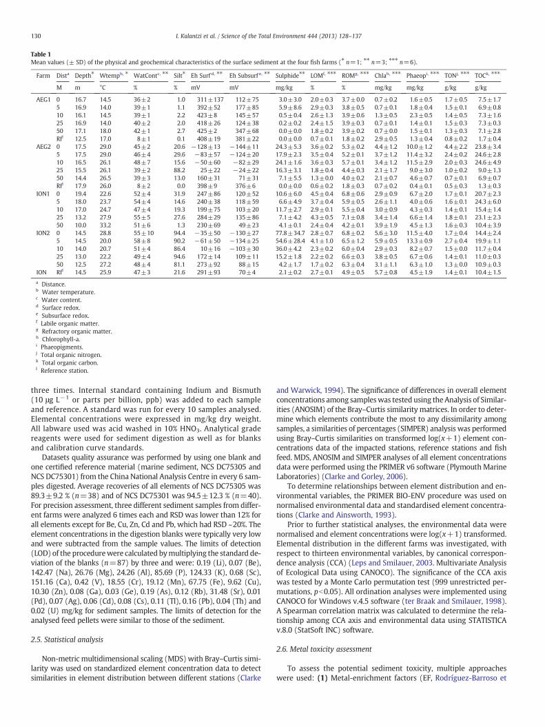
Table 1Mean values (± SD) of the physical and geochemical characteristics of the surface sediment at the four fish farms (⁎ n=1; ⁎⁎ n=3; ⁎⁎⁎ n=6).

Farm Dista Depth⁎ Wtempb, ⁎ WatContc, ⁎⁎ Silt⁎ Eh Surf d, ⁎⁎ Eh Subsurf e, ⁎⁎ Sulphide⁎⁎ LOMf, ⁎⁎⁎ ROMg, ⁎⁎⁎ Chlah, ⁎⁎⁎ Phaeopi, ⁎⁎⁎ TONj, ⁎⁎⁎ TOCk, ⁎⁎⁎

M m °C % % mV mV mg/kg % % mg/kg mg/kg g/kg g/kg

AEG1 0 16.7 14.5 36±2 1.0 311±137 112±75 3.0±3.0 2.0±0.3 3.7±0.0 0.7±0.2 1.6±0.5 1.7±0.5 7.5±1.75 16.9 14.0 39±1 1.1 392±52 177±85 5.9±8.6 2.9±0.3 3.8±0.5 0.7±0.1 1.8±0.4 1.5±0.1 6.9±0.810 16.1 14.5 39±1 2.2 423±8 145±57 0.5±0.4 2.6±1.3 3.9±0.6 1.3±0.5 2.3±0.5 1.4±0.5 7.3±1.625 16.9 14.0 40±2 2.0 418±26 124±38 0.2±0.2 2.4±1.5 3.9±0.3 0.7±0.1 1.4±0.1 1.5±0.3 7.3±0.350 17.1 18.0 42±1 2.7 425±2 347±68 0.0±0.0 1.8±0.2 3.9±0.2 0.7±0.0 1.5±0.1 1.3±0.3 7.1±2.8Rfl 12.5 17.0 8±1 0.1 408±19 381±22 0.0±0.0 0.7±0.1 1.8±0.2 2.9±0.5 1.3±0.4 0.8±0.2 1.7±0.4

AEG2 0 17.5 29.0 45±2 20.6 −128±13 −144±11 24.3±5.3 3.6±0.2 5.3±0.2 4.4±1.2 10.0±1.2 4.4±2.2 23.8±3.45 17.5 29.0 46±4 29.6 −83±57 −124±20 17.9±2.3 3.5±0.4 5.2±0.1 3.7±1.2 11.4±3.2 2.4±0.2 24.6±2.810 16.5 26.1 48±7 15.6 −50±60 −82±29 24.1±1.6 3.6±0.3 5.7±0.1 3.4±1.2 11.5±2.9 2.0±0.3 24.6±4.925 15.5 26.1 39±2 88.2 25±22 −24±22 16.3±3.1 1.8±0.4 4.4±0.3 2.1±1.7 9.0±3.0 1.0±0.2 9.0±1.350 14.4 26.5 39±3 13.0 160±31 71±31 7.1±5.5 1.3±0.0 4.0±0.2 2.1±0.7 4.6±0.7 0.7±0.1 6.9±0.7Rfl 17.9 26.0 8±2 0.0 398±9 376±6 0.0±0.0 0.6±0.2 1.8±0.3 0.7±0.2 0.4±0.1 0.5±0.3 1.3±0.3

ION1 0 19.4 22.6 52±4 31.9 247±86 120±52 10.6±6.0 4.5±0.4 6.8±0.6 2.9±0.9 6.7±2.0 1.7±0.1 20.7±2.35 18.0 23.7 54±4 14.6 240±38 118±59 6.6±4.9 3.7±0.4 5.9±0.5 2.6±1.1 4.0±0.6 1.6±0.1 24.3±6.010 17.0 24.7 47±4 19.3 199±75 103±20 11.7±2.7 2.9±0.1 5.5±0.4 3.0±0.9 4.3±0.3 1.4±0.1 15.4±1.425 13.2 27.9 55±5 27.6 284±29 135±86 7.1±4.2 4.3±0.5 7.1±0.8 3.4±1.4 6.6±1.4 1.8±0.1 23.1±2.350 10.0 33.2 51±6 1.3 230±69 49±23 4.1±0.1 2.4±0.4 4.2±0.1 3.9±1.9 4.5±1.3 1.6±0.3 10.4±3.9

ION2 0 14.5 28.8 55±10 94.4 −35±50 −130±27 77.8±34.7 2.8±0.7 6.8±0.2 5.6±3.0 11.5±4.0 1.7±0.4 14.4±2.45 14.5 20.0 58±8 90.2 −61±50 −134±25 54.6±28.4 4.1±1.0 6.5±1.2 5.9±0.5 13.3±0.9 2.7±0.4 19.9±1.110 14.0 20.7 51±4 86.4 10±16 −103±30 36.0±4.2 2.3±0.2 6.0±0.4 2.9±0.3 8.2±0.7 1.5±0.0 11.7±0.425 13.0 22.2 49±4 94.6 172±14 109±11 15.2±1.8 2.2±0.2 6.6±0.3 3.8±0.5 6.7±0.6 1.4±0.1 11.0±0.350 12.5 27.2 48±4 81.1 273±92 88±15 4.2±1.7 1.7±0.2 6.3±0.4 3.1±1.1 6.3±1.0 1.3±0.0 10.9±0.3

ION Rfl 14.5 25.9 47±3 21.6 291±93 70±4 2.1±0.2 2.7±0.1 4.9±0.5 5.7±0.8 4.5±1.9 1.4±0.1 10.4±1.5

a Distance.b Water temperature.c Water content.d Surface redox.e Subsurface redox.f Labile organic matter.g Refractory organic matter.h Chlorophyll-a.i Phaeopigments.j Total organic nitrogen.k Total organic carbon.l Reference station.

130 I. Kalantzi et al. / Science of the Total Environment 444 (2013) 128–137

three times. Internal standard containing Indium and Bismuth(10 μg L−1 or parts per billion, ppb) was added to each sampleand reference. A standard was run for every 10 samples analysed.Elemental concentrations were expressed in mg/kg dry weight.All labware used was acid washed in 10% HNO3. Analytical gradereagents were used for sediment digestion as well as for blanksand calibration curve standards.

Datasets quality assurance was performed by using one blank andone certified reference material (marine sediment, NCS DC75305 andNCS DC75301) from the China National Analysis Centre in every 6 sam-ples digested. Average recoveries of all elements of NCS DC75305 was89.3±9.2 % (n=38) and of NCS DC75301 was 94.5±12.3 % (n=40).For precision assessment, three different sediment samples from differ-ent farms were analyzed 6 times each and RSD was lower than 12% forall elements except for Be, Cu, Zn, Cd and Pb, which had RSD ~20%. Theelement concentrations in the digestion blanks were typically very lowand were subtracted from the sample values. The limits of detection(LOD) of the procedurewere calculated bymultiplying the standard de-viation of the blanks (n=87) by three and were: 0.19 (Li), 0.07 (Be),142.47 (Na), 26.76 (Mg), 24.26 (Al), 85.69 (P), 124.33 (K), 0.68 (Sc),151.16 (Ca), 0.42 (V), 18.55 (Cr), 19.12 (Mn), 67.75 (Fe), 9.62 (Cu),10.30 (Zn), 0.08 (Ga), 0.03 (Ge), 0.19 (As), 0.12 (Rb), 31.48 (Sr), 0.01(Pd), 0.07 (Ag), 0.06 (Cd), 0.08 (Cs), 0.11 (Tl), 0.16 (Pb), 0.04 (Th) and0.02 (U) mg/kg for sediment samples. The limits of detection for theanalysed feed pellets were similar to those of the sediment.

2.5. Statistical analysis

Non-metric multidimensional scaling (MDS) with Bray–Curtis simi-larity was used on standardized element concentration data to detectsimilarities in element distribution between different stations (Clarke

and Warwick, 1994). The significance of differences in overall elementconcentrations among sampleswas tested using the Analysis of Similar-ities (ANOSIM) of the Bray–Curtis similarity matrices. In order to deter-mine which elements contribute the most to any dissimilarity amongsamples, a similarities of percentages (SIMPER) analysis was performedusing Bray–Curtis similarities on transformed log(x+1) element con-centrations data of the impacted stations, reference stations and fishfeed. MDS, ANOSIM and SIMPER analyses of all element concentrationsdata were performed using the PRIMER v6 software (Plymouth MarineLaboratories) (Clarke and Gorley, 2006).

To determine relationships between element distribution and en-vironmental variables, the PRIMER BIO-ENV procedure was used onnormalised environmental data and standardised element concentra-tions (Clarke and Ainsworth, 1993).

Prior to further statistical analyses, the environmental data werenormalised and element concentrations were log(x+1) transformed.Elemental distribution in the different farms was investigated, withrespect to thirteen environmental variables, by canonical correspon-dence analysis (CCA) (Leps and Smilauer, 2003. Multivariate Analysisof Ecological Data using CANOCO). The significance of the CCA axiswas tested by a Monte Carlo permutation test (999 unrestricted per-mutations, pb0.05). All ordination analyses were implemented usingCANOCO for Windows v.4.5 software (ter Braak and Smilauer, 1998).A Spearman correlation matrix was calculated to determine the rela-tionship among CCA axis and environmental data using STATISTICAv.8.0 (StatSoft INC) software.

2.6. Metal toxicity assessment

To assess the potential sediment toxicity, multiple approacheswere used: (1) Metal-enrichment factors (EF, Rodríguez-Barroso et

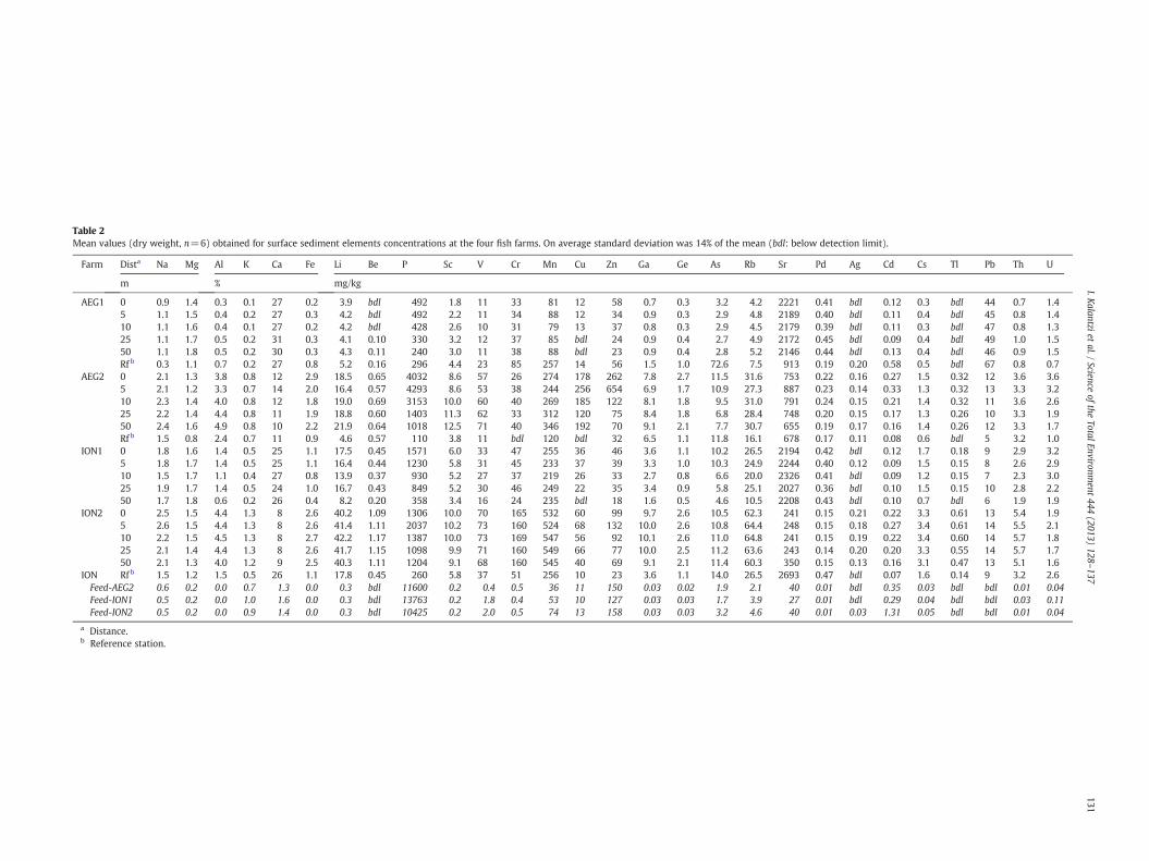
Table 2Mean values (dry weight, n=6) obtained for surface sediment elements concentrations at the four fish farms. On average standard deviation was 14% of the mean (bdl: below detection limit).

Farm Dista Na Mg Al K Ca Fe Li Be P Sc V Cr Mn Cu Zn Ga Ge As Rb Sr Pd Ag Cd Cs Tl Pb Th U

m % mg/kg

AEG1 0 0.9 1.4 0.3 0.1 27 0.2 3.9 bdl 492 1.8 11 33 81 12 58 0.7 0.3 3.2 4.2 2221 0.41 bdl 0.12 0.3 bdl 44 0.7 1.45 1.1 1.5 0.4 0.2 27 0.3 4.2 bdl 492 2.2 11 34 88 12 34 0.9 0.3 2.9 4.8 2189 0.40 bdl 0.11 0.4 bdl 45 0.8 1.410 1.1 1.6 0.4 0.1 27 0.2 4.2 bdl 428 2.6 10 31 79 13 37 0.8 0.3 2.9 4.5 2179 0.39 bdl 0.11 0.3 bdl 47 0.8 1.325 1.1 1.7 0.5 0.2 31 0.3 4.1 0.10 330 3.2 12 37 85 bdl 24 0.9 0.4 2.7 4.9 2172 0.45 bdl 0.09 0.4 bdl 49 1.0 1.550 1.1 1.8 0.5 0.2 30 0.3 4.3 0.11 240 3.0 11 38 88 bdl 23 0.9 0.4 2.8 5.2 2146 0.44 bdl 0.13 0.4 bdl 46 0.9 1.5Rf b 0.3 1.1 0.7 0.2 27 0.8 5.2 0.16 296 4.4 23 85 257 14 56 1.5 1.0 72.6 7.5 913 0.19 0.20 0.58 0.5 bdl 67 0.8 0.7

AEG2 0 2.1 1.3 3.8 0.8 12 2.9 18.5 0.65 4032 8.6 57 26 274 178 262 7.8 2.7 11.5 31.6 753 0.22 0.16 0.27 1.5 0.32 12 3.6 3.65 2.1 1.2 3.3 0.7 14 2.0 16.4 0.57 4293 8.6 53 38 244 256 654 6.9 1.7 10.9 27.3 887 0.23 0.14 0.33 1.3 0.32 13 3.3 3.210 2.3 1.4 4.0 0.8 12 1.8 19.0 0.69 3153 10.0 60 40 269 185 122 8.1 1.8 9.5 31.0 791 0.24 0.15 0.21 1.4 0.32 11 3.6 2.625 2.2 1.4 4.4 0.8 11 1.9 18.8 0.60 1403 11.3 62 33 312 120 75 8.4 1.8 6.8 28.4 748 0.20 0.15 0.17 1.3 0.26 10 3.3 1.950 2.4 1.6 4.9 0.8 10 2.2 21.9 0.64 1018 12.5 71 40 346 192 70 9.1 2.1 7.7 30.7 655 0.19 0.17 0.16 1.4 0.26 12 3.3 1.7Rf b 1.5 0.8 2.4 0.7 11 0.9 4.6 0.57 110 3.8 11 bdl 120 bdl 32 6.5 1.1 11.8 16.1 678 0.17 0.11 0.08 0.6 bdl 5 3.2 1.0

ION1 0 1.8 1.6 1.4 0.5 25 1.1 17.5 0.45 1571 6.0 33 47 255 36 46 3.6 1.1 10.2 26.5 2194 0.42 bdl 0.12 1.7 0.18 9 2.9 3.25 1.8 1.7 1.4 0.5 25 1.1 16.4 0.44 1230 5.8 31 45 233 37 39 3.3 1.0 10.3 24.9 2244 0.40 0.12 0.09 1.5 0.15 8 2.6 2.910 1.5 1.7 1.1 0.4 27 0.8 13.9 0.37 930 5.2 27 37 219 26 33 2.7 0.8 6.6 20.0 2326 0.41 bdl 0.09 1.2 0.15 7 2.3 3.025 1.9 1.7 1.4 0.5 24 1.0 16.7 0.43 849 5.2 30 46 249 22 35 3.4 0.9 5.8 25.1 2027 0.36 bdl 0.10 1.5 0.15 10 2.8 2.250 1.7 1.8 0.6 0.2 26 0.4 8.2 0.20 358 3.4 16 24 235 bdl 18 1.6 0.5 4.6 10.5 2208 0.43 bdl 0.10 0.7 bdl 6 1.9 1.9

ION2 0 2.5 1.5 4.4 1.3 8 2.6 40.2 1.09 1306 10.0 70 165 532 60 99 9.7 2.6 10.5 62.3 241 0.15 0.21 0.22 3.3 0.61 13 5.4 1.95 2.6 1.5 4.4 1.3 8 2.6 41.4 1.11 2037 10.2 73 160 524 68 132 10.0 2.6 10.8 64.4 248 0.15 0.18 0.27 3.4 0.61 14 5.5 2.110 2.2 1.5 4.5 1.3 8 2.7 42.2 1.17 1387 10.0 73 169 547 56 92 10.1 2.6 11.0 64.8 241 0.15 0.19 0.22 3.4 0.60 14 5.7 1.825 2.1 1.4 4.4 1.3 8 2.6 41.7 1.15 1098 9.9 71 160 549 66 77 10.0 2.5 11.2 63.6 243 0.14 0.20 0.20 3.3 0.55 14 5.7 1.750 2.1 1.3 4.0 1.2 9 2.5 40.3 1.11 1204 9.1 68 160 545 40 69 9.1 2.1 11.4 60.3 350 0.15 0.13 0.16 3.1 0.47 13 5.1 1.6

ION Rf b 1.5 1.2 1.5 0.5 26 1.1 17.8 0.45 260 5.8 37 51 256 10 23 3.6 1.1 14.0 26.5 2693 0.47 bdl 0.07 1.6 0.14 9 3.2 2.6Feed-AEG2 0.6 0.2 0.0 0.7 1.3 0.0 0.3 bdl 11600 0.2 0.4 0.5 36 11 150 0.03 0.02 1.9 2.1 40 0.01 bdl 0.35 0.03 bdl bdl 0.01 0.04Feed-ION1 0.5 0.2 0.0 1.0 1.6 0.0 0.3 bdl 13763 0.2 1.8 0.4 53 10 127 0.03 0.03 1.7 3.9 27 0.01 bdl 0.29 0.04 bdl bdl 0.03 0.11Feed-ION2 0.5 0.2 0.0 0.9 1.4 0.0 0.3 bdl 10425 0.2 2.0 0.5 74 13 158 0.03 0.03 3.2 4.6 40 0.01 0.03 1.31 0.05 bdl bdl 0.01 0.04

a Distance.b Reference station.

131I.K

alantzietal./

Scienceofthe

TotalEnvironment

444(2013)

128–137

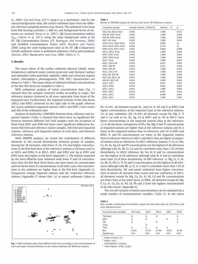
Table 3Results of ANOSIM analysis for the four fish farms (Rf: Reference station).

Compared groups Sample statistic (Global R) Statistic — R pb

AEG2-Rf, AEG2-Feed 0.956 1.000 0.012ION-Rf, ION1-Feed 0.956 1.000 0.002ION-Rf, ION2-Feed 0.956 1.000 0.002AEG1-Rf, Feed 0.956 1.000 0.001AEG2-Feed, ION2-Feed 0.956 0.000 nsAEG2-Feed, ION1-Feed 0.956 0.154 nsION2-Feed, ION1-Feed 0.956 0.400 0.009AEG2, AEG2-Feed 0.956 1.000 0.001ION1, ION1-Feed 0.956 1.000 0.001ION2, ION2-Feed 0.956 1.000 0.001AEG1, Feed 0.956 1.000 0.001AEG2, AEG2-Rf 0.954 0.925 0.001ION1, ION-Rf 0.954 0.241 0.039ION2, ION-Rf 0.954 1.000 0.001AEG1, AEG1-Rf 0.954 1.000 0.001AEG2-Rf, ION-Rf 0.954 1.000 0.002AEG2-Rf, AEG1-Rf 0.954 1.000 0.002ION-Rf, AEG1-Rf 0.954 1.000 0.002AEG2, ION1 0.954 0.901 0.001AEG2, ION2 0.954 0.845 0.001AEG2, AEG1 0.954 1.000 0.001ION2, ION1 0.954 0.997 0.001ION1, AEG1 0.954 0.948 0.001ION2, AEG1 0.954 1.000 0.001

132 I. Kalantzi et al. / Science of the Total Environment 444 (2013) 128–137

al., 2009; Yap and Pang, 2011) using Li as a normaliser; and for thenatural background value, the surface sediment layer from the differ-ent reference sampling stations was chosen. This sediment is far awayfrom fish farming activities (>400 m) and background levels of ele-ments are reached (Dean et al., 2007); (2) Geoaccumulation indices(Igeo, Cukrov et al., 2011) using the same background value as forEF; (3) Contamination factors (CF, Rodrigues and Formoso, 2006)and modified Contamination Factor (mCF, Abrahim and Parker,2008) using the same background value as for EF; (4) Comparisonsof bulk-sediment values to published sediment criteria and standards(Burton, 2002; Bjørgesæter and Gray, 2008; Tables 6, 7).

3. Results

The mean values of the surface sediment physical (depth, watertemperature, sedimentwater content, grain size) and chemical (surfaceand subsurface redox potential, sulphides, labile and refractory organicmatter, chlorophyll-a, phaeopigments, TON, TOC) characteristics areshown in Table 1. Themean values of sediment element concentrationsat the four fish farms are included in Table 2.

MDS ordination analysis of metal concentration data (Fig. 1)showed that the samples clustered visibly according to origin. Thereference stations clustered in all cases separately from those of theimpacted ones. Furthermore, the impacted stations of the silty farms(AEG2 and ION2) clustered on the right side of the graph, whereasthe coarse-sediment impacted stations (AEG1 and ION1) were centerand left of the ordination plot.

Analysis of similarities (ANOSIM) between feed, reference and im-pacted stations (Table 3) showed that there were no significant dif-ferences between different fish feed samples with the exception offeeds from ION1 and ION2 but there were significant differences be-tween fish feed and reference station samples, fish feed and impactedstations, reference and impacted stations at each farm, and betweenreference stations.

With SIMPER analysis, we tested the contribution of differentelements to the overall dissimilarity between groups of samples.Among the 28 elements, only three (P, Zn, Cd) had higher concentra-tions in the fish feed than at the reference stations at all farms and Cuat AEG2 and ION2, K at AEG1, ION1 and ION2 and Ag at ION1 andION2 were also higher in the feed (Appendix 1). The stations impactedby the farm effluents have sediment with lower P and Cd concentra-tions than the fish feed, three farms also have lower Zn concentrationand two farms lower K concentrations. In all other cases, the concentra-tions in the sediment are higher than in the fish feed (Appendix 2).Comparison among impacted stations and the respective referencestations (Appendix 3) shows that: (a) in anoxic sediments (taken as

AreasAEG1AEG2ION1ION2AEG1-RfAEG2-RfION-Rf

2D Stress: 0,06

Fig. 1. MDS ordination plot of the different fish farms according to the concentrations oftrace and major chemical elements in the surface sediment (Rf: Reference station).

Ehb0 mV), all elements except As, (and Ca, Sr, Pd and U at ION2) hadhigher concentrations at the impacted than at the reference stations;(b) in oxic sediments (Eh>0 mV) all elements except Na, Mg, P, Tland U (as well as Cu, Zn, Ag, Cd at ION1 and Sr, Pd at AEG1) havelower concentrations at the impacted stations than at the reference;(c) in all the farms (irrespective of Eh), Na, Mg, P and Tl concentrationsat impacted stations are higher than at the reference stations and As islower at the impacted stations than in references, and (d) in ION1 andION2, Sr and Pd concentrations are lower in the impacted stationsthan in referencewhereas in AEG1 and AEG2, they are higher at impact-ed stations than at references. In AEG1 reference stations, P, Ca, Cr, Mn,Cu, Zn, As, Ag, Cd and Pb concentrations are the highest of all referencesalthough only As, Pb, Cr, Cu and Zn contribute more than 1.5% of theirdissimilarity. In AEG2 reference, Be, Na, Al, K and Ga concentrationsare the highest of all references although only Al, K and Ga contributemore than 2% of their dissimilarity. In ION reference, Li, Mg, Sc, V, Fe,Ge, Rb, Sr, Pd, Cs, Tl, Th and U concentrations are the highest of all refer-ences although only Rb, Li, Sr, U, V and Cs contribute more than 1.5% oftheir dissimilarity. Silt and anoxic sediments have higher concentra-tions of almost all elements than coarse and oxic sediments. In AEG1,all elements except for Mg, Ca, Zn, Sr, Pd, Cd and Pb, concentrationsare lower than at the other farms. In ION2, all elements except for Mg,P, Ca, Sc, Cu, Zn, Sr, Pd, Cd, Pb and U have the highest concentrationsof all other farms (Appendix 4).

The overall variance of metal concentrations can be explained by asmall number of environmental variables (Table 4). In the entire

Table 4Best variable combination from BioEnv analysis for the entire date set (All Farms) andeach individual farm.

Environmental variables All Farms AEG1 AEG2 ION1 ION2

aWCont% X X X XSilt% X X X XbEh X X XcChla XdTOC X X X XRho 0.583 0.734 0.769 0.632 0.745Significance 0.01 0.01 0.01 0.01 0.01

a Water Content (%).b Redox (mV).c Chlorophyll-a (mg/kg).d Total organic carbon (g/kg).

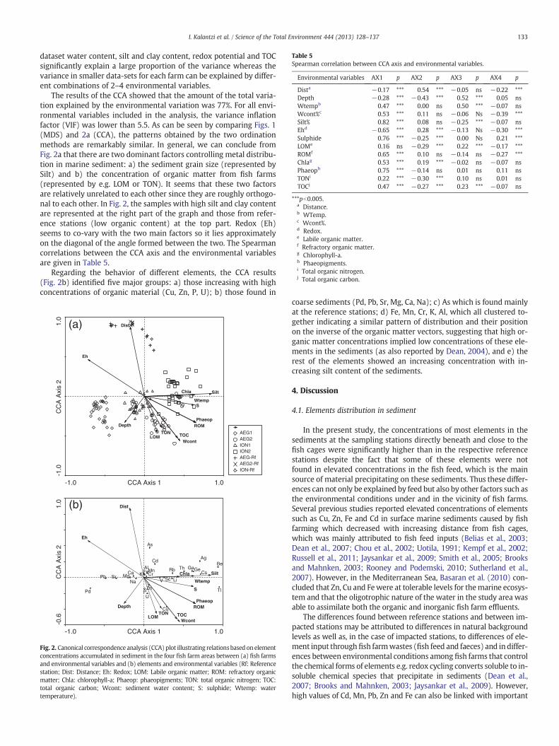
Table 5Spearman correlation between CCA axis and environmental variables.

Environmental variables AX1 p AX2 p AX3 p AX4 p

Dista −0.17 *** 0.54 *** −0.05 ns −0.22 ***Depth −0.28 *** −0.43 *** 0.52 *** 0.05 nsWtempb 0.47 *** 0.00 ns 0.50 *** −0.07 nsWcont%c 0.53 *** 0.11 ns −0.06 Ns −0.39 ***Silt% 0.82 *** 0.08 ns −0.25 *** −0.07 nsEhd −0.65 *** 0.28 *** −0.13 Ns −0.30 ***Sulphide 0.76 *** −0.25 *** 0.00 Ns 0.21 ***LOMe 0.16 ns −0.29 *** 0.22 *** −0.17 ***ROMf 0.65 *** 0.10 ns −0.14 ns −0.27 ***Chlag 0.53 *** 0.19 *** −0.02 ns −0.07 nsPhaeoph 0.75 *** −0.14 ns 0.01 ns 0.11 nsTONi 0.22 *** −0.30 *** 0.10 ns 0.01 nsTOCj 0.47 *** −0.27 *** 0.23 *** −0.07 ns

***pb0.005.a Distance.b WTemp.c Wcont%.d Redox.e Labile organic matter.f Refractory organic matter.g Chlorophyll-a.h Phaeopigments.i Total organic nitrogen.j Total organic carbon.

133I. Kalantzi et al. / Science of the Total Environment 444 (2013) 128–137

dataset water content, silt and clay content, redox potential and TOCsignificantly explain a large proportion of the variance whereas thevariance in smaller data-sets for each farm can be explained by differ-ent combinations of 2–4 environmental variables.

The results of the CCA showed that the amount of the total varia-tion explained by the environmental variation was 77%. For all envi-ronmental variables included in the analysis, the variance inflationfactor (VIF) was lower than 5.5. As can be seen by comparing Figs. 1(MDS) and 2a (CCA), the patterns obtained by the two ordinationmethods are remarkably similar. In general, we can conclude fromFig. 2a that there are two dominant factors controlling metal distribu-tion in marine sediment: a) the sediment grain size (represented bySilt) and b) the concentration of organic matter from fish farms(represented by e.g. LOM or TON). It seems that these two factorsare relatively unrelated to each other since they are roughly orthogo-nal to each other. In Fig. 2, the samples with high silt and clay contentare represented at the right part of the graph and those from refer-ence stations (low organic content) at the top part. Redox (Eh)seems to co-vary with the two main factors so it lies approximatelyon the diagonal of the angle formed between the two. The Spearmancorrelations between the CCA axis and the environmental variablesare given in Table 5.

Regarding the behavior of different elements, the CCA results(Fig. 2b) identified five major groups: a) those increasing with highconcentrations of organic material (Cu, Zn, P, U); b) those found in

-1.0 CCA Axis 1 1.0

Li

Be

NaMg

Al

P

KSc

Ca

VCrMnFe

Cu

Zn

GaGe

As

Rb

Sr

Pd

AgCd

Cs

Tl

Pb

Th

U

Dist

Depth

Wtemp

Wcont

Silt

Eh

S

LOM

ROM

Chla

Phaeop

TON TOC

-1.0 CCA Axis 1 1.0

Dist

Depth

Wtemp

Wcont

Silt

Eh

S

LOM

ROM

Chla

Phaeop

TON TOC AEG1AEG2ION1ION2AEG-RfAEG2-RfION-Rf

CC

A A

xis

2

(a)

(b)

CC

A A

xis

2-0

.61.

0-1

.0

1.0

Fig. 2. Canonical correspondence analysis (CCA) plot illustrating relationsbased on elementconcentrations accumulated in sediment in the four fish farm areas between (a) fish farmsand environmental variables and (b) elements and environmental variables (Rf: Referencestation; Dist: Distance; Eh: Redox; LOM: Labile organic matter; ROM: refractory organicmatter; Chla: chlorophyll-a; Phaeop: phaeopigments; TON: total organic nitrogen; TOC:total organic carbon; Wcont: sediment water content; S: sulphide; Wtemp: watertemperature).

coarse sediments (Pd, Pb, Sr, Mg, Ca, Na); c) As which is found mainlyat the reference stations; d) Fe, Mn, Cr, K, Al, which all clustered to-gether indicating a similar pattern of distribution and their positionon the inverse of the organic matter vectors, suggesting that high or-ganic matter concentrations implied low concentrations of these ele-ments in the sediments (as also reported by Dean, 2004), and e) therest of the elements showed an increasing concentration with in-creasing silt content of the sediments.

4. Discussion

4.1. Elements distribution in sediment

In the present study, the concentrations of most elements in thesediments at the sampling stations directly beneath and close to thefish cages were significantly higher than in the respective referencestations despite the fact that some of these elements were notfound in elevated concentrations in the fish feed, which is the mainsource of material precipitating on these sediments. Thus these differ-ences can not only be explained by feed but also by other factors such asthe environmental conditions under and in the vicinity of fish farms.Several previous studies reported elevated concentrations of elementssuch as Cu, Zn, Fe and Cd in surface marine sediments caused by fishfarming which decreased with increasing distance from fish cages,which was mainly attributed to fish feed inputs (Belias et al., 2003;Dean et al., 2007; Chou et al., 2002; Uotila, 1991; Kempf et al., 2002;Russell et al., 2011; Jaysankar et al., 2009; Smith et al., 2005; Brooksand Mahnken, 2003; Rooney and Podemski, 2010; Sutherland et al.,2007). However, in the Mediterranean Sea, Basaran et al. (2010) con-cluded that Zn, Cu and Fewere at tolerable levels for themarine ecosys-tem and that the oligotrophic nature of the water in the study area wasable to assimilate both the organic and inorganic fish farm effluents.

The differences found between reference stations and between im-pacted stations may be attributed to differences in natural backgroundlevels as well as, in the case of impacted stations, to differences of ele-ment input through fish farmwastes (fish feed and faeces) and in differ-ences between environmental conditions among fish farms that controlthe chemical forms of elements e.g. redox cycling converts soluble to in-soluble chemical species that precipitate in sediments (Dean et al.,2007; Brooks and Mahnken, 2003; Jaysankar et al., 2009). However,high values of Cd, Mn, Pb, Zn and Fe can also be linked with important

134 I. Kalantzi et al. / Science of the Total Environment 444 (2013) 128–137

anthropogenic input through atmospheric emission, fly ash, domesticand industrial effluent discharge and, extensive use of antifouling paintsby shipping activities (Sarkar et al., 2004).

Previous studies of geochemical variables with sediment profiles(Karakassis et al., 1998) or spatial changes with transects (Karakassis etal., 2000; Lampadariou et al., 2005; Papageorgiou et al., 2010) haveshown that the effects of fish farming on organic matter, redox potentialand sediment texture is negligible beyond 25–50 m from the edge of thecages. Russell et al. (2011) concluded that any impact from organic pol-lutants or trace elements is of a local nature. Results of the presentstudy agree with this conclusion as the effects of aquaculture on sedi-ment elements distribution was negligible 25–50 m away from the fishcages. Other studies reported that the effects of the accumulation of Zn,Cu, P and Ca in sediments are reduced at the 50–100 m (Chou et al.,2002; Smith et al., 2005; Brooks and Mahnken, 2003; Schendel et al.,2004) or 200 m (Smith et al., 2005) stations compared to stationsunder the cages.

4.2. Fish farms effluents and elements concentrations in sediment

Surface sediment composition under and in the vicinity of the cagesis continuously changing depending on the composition of the solidscontained in aquaculture effluents (Mendiguchía et al., 2006). The sea-bed near and around fish farms is covered by a sludgewhich is enrichedwith colloidal organic carbon and tracemetalswhich comemainly fromunused fish feed (Belias et al., 2003). Following biodegradation of thissludge, anoxic conditions are created followed by the formation of un-desirable gases, precipitation or remobilization of elements and the ex-tinction of most macrobenthic fauna (Belias et al., 2003).

In the present study, it was found that P, Cd, Zn and K had higherconcentrations in the fish feed than at the impacted and unimpactedstations. This indicates that the input of these four elements in the ma-rine environment is higher than background values and therefore sedi-ment enrichment of these elements is expected near and around fishcages through organic matter accumulation and redox cycling. This isin agreement with the hypothesis that the sedimentation of uneatenfeed and faeces is the main source of Zn, P and Cd whereas the majorityof Cu concentrations come from another source (e.g. antifoulants)which depends strongly on the frequency of net maintenance andhydrodynamism in each farm. This was also found by Dean et al.(2007), Uotila (1991), Chou et al. (2002), Belias et al. (2003), Basaranet al. (2010), Wu and Yang (2010). Perhaps this is less so in the caseof K which is abundant in sea water and rock although it has beenfound that organic matter enhances the rate of K adsorption in soils(Wang and Huang, 2001).

Elements are present in fish feed either as constituents of the mealfrom which the diet is manufactured or are added for nutritional pur-poses. The elements in feed include, among others, Cu, Zn, Fe, Mn, Co,As, Mg and Se (Burridge et al., 2010; Grigorakis and Rigos, 2011). Inparticular, Zn and Cu have been found in high concentrations in fishfeed samples (Chou et al., 2002; Pergent et al., 1999) whereas Pb(Mendiguchía et al., 2006), Fe, Mn and Al were found to be at verylow levels in comparison to background sediment levels (Jaysankaret al., 2009). The high P sedimentation reported is probably due toexcessive dietary P content and low P retention by aquatic animals(Wu and Yang, 2010; Schendel et al., 2004; Smith et al., 2005).

Most published information on metals in fish farm sediments alsoinvolves analysis of the fish feed supplied, the present paper is no ex-ception to that. However, it should be noted that there are some lim-itations regarding comparisons among these two types of matrix. Theconcentrations vary, but so do the quantities of sediments accumulat-ed beneath farms and the precipitating feed and faeces. In this con-text, the concentration of the fish feed provides an indication of theinput provided by the farming activity but this input is modified by se-lective assimilation of elements in the fish (for the eaten part of thefeed) and by chemical processes in thewater column and the sediment.

In otherwords, the feed and the sediment are not a closed systembut anopen systemwhere dissolvedmetals are scavenged by or released fromsediments depending on the geochemical conditions.

4.3. Environmental variables and elements distribution in sediment

In addition to the major input from uneaten feed and faeces, floccu-lents, naturally occurring organic debris andMn and Fe oxy-hydroxidesregulated by redox regime may also contribute to sediment elementconcentrations around the fish cages (Chou et al., 2002; Dean et al.,2007). Thus, separating naturally occurring concentrations of elementsfrom those influenced by anthropogenic activities is a very challengingtask given the natural variability of elements observed in backgroundcoastal sediments, influenced largely by granulometric, mineralogicaland organic factors (Sutherland et al., 2007).

The fish farms investigated in the present study showed charac-teristics typical of Mediterranean fish farms found in previous studies(Karakassis et al., 2000; Kalantzi and Karakassis, 2006) spanning fromcoarse oxidized sediments to silty reduced ones. According to thepresent study, elemental distribution may be explained by the signif-icant changes in sediment texture (silt %), organic content and redoxregime which drastically affect their behavior. This has also beenshown for some elements by other authors (Sutherland et al., 2007;Han et al., 1996; Peltola et al., 2011; Mayor and Solan, 2011; Chouet al., 2002). It was concluded that elements in sediments near andaround fish farms can be clustered into five groups according to or-ganic matter, sediment grain size and distance from the cages. Onegroup (Cu, Zn, P, U) is found in organic enriched, anoxic sedimentwith a high water content that occurs near the cages; a secondgroup (Pd, Pb, Sr, Mg, Ca, Na) is related to coarse, oxic sediments; athird group (As) is associated with sediments from the reference sta-tions; the fourth (Fe, Mn, Cr, K, Al) is associated with organic-poorsediment with low water content; and the fifth (Cd, V, Sc, Li, Rb, Th,Ga, Ge, Cs, Ag, Be, Tl) is found in fine grained, sulfur-rich sedimentswith high silt content. It can be concluded that grain size and organicmatter are the main factors that control element distribution. Ele-ment clustering can be attributed to aquaculture activities in termsof the released wastes and the induced environmental conditions.

Contaminants have different affinities for the various binding siteswithin the sediment. The majority of metal contaminants partition ontoparticulate matter such as clay minerals, Fe and Mn oxy-hydroxides(e.g. Pb, Cd, Cr), exchangeable cations/ carbonates (e.g. Cd), sulphides(e.g. Cu, Zn), organic substances such as humic acids (e.g. Cu, Cd) andbiological materials such as algae and bacteria (U) (Eggleton andThomas, 2004; Sutherland et al., 2007; Brooks and Mahnken, 2003;Prego and Cobelo-García, 2003; Smith et al., 2005; Siegel et al., 1994).

The role of sediment in chemical pollution is tied both to particle sizeand to the amount of particulate organic carbon associatedwith the sed-iment (Islam and Tanaka, 2004). The smaller the grain size (clay or silt)and thehigher the organic content and the percentages of iron andman-ganese, the more effectively the sediment is able to scavenge the ele-ments (Han et al., 1996; Brooks andMahnken, 2003; Sarkar et al., 2004).

Certainmetals have an associationwith organicmatter which can beexplained by thewell-known high affinity of thesemetals, especially Cu,Zn and Pb, to humic substances which are a fraction of natural organicmatter (Sekhar et al., 2003). Humic substances have a high content ofoxygen-donor ligand, such as carboxyls and phenolic OH groups(Astrom and Corin, 2000; Decho and Luoma, 1994) which form com-plexes with metal ions and thereby affect metal mobility in the aquaticenvironment. Incoming dissolved metals are scavenged by the organicligands and may then be precipitated as organo-metallic complexes(Dean, 2004). Many elements complex with organic matter andcoprecipitate with sulphide species in anoxic conditions (Sutherland etal., 2007; Siegel et al., 1994; Roach et al., 2008; Sarkar et al., 2004).

Sediments with high concentrations of Fe and Mn oxy-hydroxidescan scavenge elements (As, Cd, Cu, Mn and Zn, and to a lesser extent

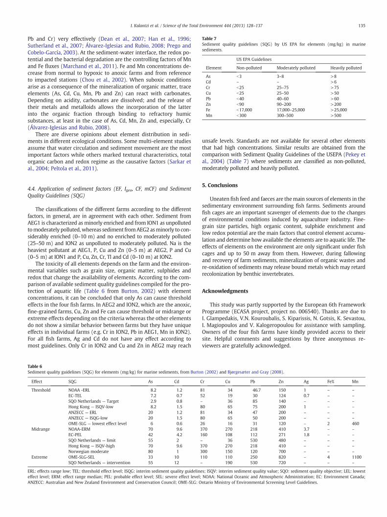
Table 7Sediment quality guidelines (SQG) by US EPA for elements (mg/kg) in marinesediments.

US EPA Guidelines

Element Non-polluted Moderately polluted Heavily polluted

As b3 3–8 >8Cd – – >6Cr b25 25–75 >75Cu b25 25–50 >50Pb b40 40–60 >60Zn b90 90–200 >200Fe b17,000 17,000–25,000 >25,000Mn b300 300–500 >500

135I. Kalantzi et al. / Science of the Total Environment 444 (2013) 128–137

Pb and Cr) very effectively (Dean et al., 2007; Han et al., 1996;Sutherland et al., 2007; Álvarez-Iglesias and Rubio, 2008; Prego andCobelo-García, 2003). At the sediment-water interface, the redox po-tential and the bacterial degradation are the controlling factors of Mnand Fe fluxes (Marchand et al., 2011). Fe and Mn concentrations de-crease from normal to hypoxic to anoxic farms and from referenceto impacted stations (Chou et al., 2002). When suboxic conditionsarise as a consequence of the mineralization of organic matter, traceelements (As, Cd, Cu, Mn, Pb and Zn) can react with carbonates.Depending on acidity, carbonates are dissolved; and the release oftheir metals and metalloids allows the incorporation of the latterinto the organic fraction through binding to refractory humicsubstances, at least in the case of As, Cd, Mn, Zn and, especially, Cr(Álvarez-Iglesias and Rubio, 2008).

There are diverse opinions about element distribution in sedi-ments in different ecological conditions. Some multi-element studiesassume that water circulation and sediment movement are the mostimportant factors while others marked textural characteristics, totalorganic carbon and redox regime as the causative factors (Sarkar etal., 2004; Peltola et al., 2011).

4.4. Application of sediment factors (EF, Igeo, CF, mCF) and SedimentQuality Guidelines (SQG)

The classifications of the different farms according to the differentfactors, in general, are in agreement with each other. Sediment fromAEG1 is characterized as minorly enriched and from ION1 as unpollutedtomoderately polluted,whereas sediment fromAEG2 asminorly to con-siderably enriched (0–10 m) and no enriched to moderately polluted(25–50 m) and ION2 as unpolluted to moderately polluted. Na is theheaviest pollutant at AEG1, P, Cu and Zn (0–5 m) at AEG2, P and Cu(0–5 m) at ION1 and P, Cu, Zn, Cr, Tl and Cd (0–10 m) at ION2.

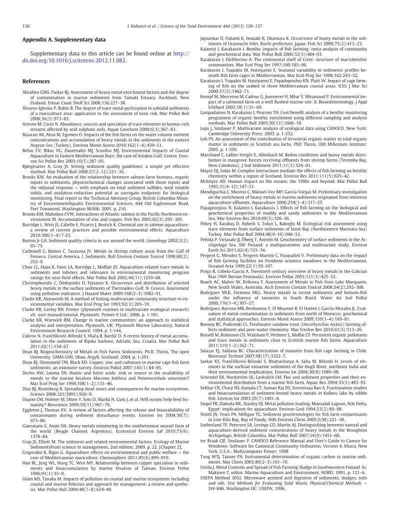
The toxicity of all elements depends on the farm and the environ-mental variables such as grain size, organic matter, sulphides andredox that change the availability of elements. According to the com-parison of available sediment quality guidelines compiled for the pro-tection of aquatic life (Table 6 from Burton, 2002) with elementconcentrations, it can be concluded that only As can cause thresholdeffects in the four fish farms. In AEG2 and ION2, which are the anoxic,fine-grained farms, Cu, Zn and Fe can cause threshold or midrange orextreme effects depending on the criteria whereas the other elementsdo not show a similar behavior between farms but they have uniqueeffects in individual farms (e.g. Cr in ION2, Pb in AEG1, Mn in ION2).For all fish farms, Ag and Cd do not have any effect according tomost guidelines. Only Cr in ION2 and Cu and Zn in AEG2 may reach

Table 6Sediment quality guidelines (SQG) for elements (mg/kg) for marine sediments, from Burto

Effect SQG As Cd C

Threshold NOAA -ERL 8.2 1.2 8EC-TEL 7.2 0.7 5SQO Netherlands — Target 2.9 0.8 –

Hong Kong — ISQV-low 8.2 1.5 8ANZECC — ERL 20 1.2 8ANZECC — ISQG-low 20 1.5 8OME-SLG — lowest effect level 6 0.6 2

Midrange NOAA-ERM 70 9.6 3EC-PEL 42 4.2 1SQO Netherlands — limit 55 2 –

Hong Kong — ISQV-high 70 9.6 3Norwegian moderate 80 1 3

Extreme OME-SLG-SEL 33 10 1SQO Netherlands — intervention 55 12 –

ERL: effects range low; TEL: threshold effect level; ISQG: interim sediment quality guidelineeffect level; ERM: effect range median; PEL: probable effect level; SEL: severe effect level;ANZECC: Australian and New Zealand Environment and Conservation Council; OME-SLG: O

unsafe levels. Standards are not available for several other elementsthat had high concentrations. Similar results are obtained from thecomparison with Sediment Quality Guidelines of the USEPA (Pekey etal., 2004) (Table 7) where sediments are classified as non-polluted,moderately polluted and heavily polluted.

5. Conclusions

Uneaten fish feed and faeces are themain sources of elements in thesedimentary environment surrounding fish farms. Sediments aroundfish cages are an important scavenger of elements due to the changesof environmental conditions induced by aquaculture industry. Fine-grain size particles, high organic content, sulphide enrichment andlow redox potential are the main factors that control element accumu-lation and determine how available the elements are to aquatic life. Theeffects of elements on the environment are only significant under fishcages and up to 50 m away from them. However, during fallowingand recovery of farm sediments, mineralization of organic wastes andre-oxidation of sediments may release bound metals which may retardrecolonization by benthic invertebrates.

Acknowledgments

This study was partly supported by the European 6th FrameworkProgramme (ECASA project, project no. 006540). Thanks are due toI. Glampedakis, V.N. Kouroubalis, S. Kiparissis, N. Gotsis, K. Sevastou,I. Magiopoulos and V. Kalogeropoulou for assistance with sampling.Owners of the four fish farms have kindly provided access to theirsite. Helpful comments and suggestions by three anonymous re-viewers are gratefully acknowledged.

n (2002) and Bjørgesæter and Gray (2008).

r Cu Pb Zn Ag Fe% Mn

1 34 46.7 150 1 – –

2 19 30 124 0.7 – –

36 85 140 – – –

0 65 75 200 1 – –

1 34 47 200 – – –

0 65 50 200 – – –

6 16 31 120 – 2 46070 270 218 410 3.7 – –

60 108 112 271 1.8 – –

36 530 480 – – –

70 270 218 410 – – –

00 150 120 700 – – –

10 110 250 820 – 4 1100190 530 720 – – –

s; ISQV: interim sediment quality value; SQO: sediment quality objective; LEL: lowestNOAA: National Oceanic and Atmospheric Administration; EC: Environment Canada;ntario Ministry of Environmental Screening Level Guidelines.

136 I. Kalantzi et al. / Science of the Total Environment 444 (2013) 128–137

Appendix A. Supplementary data

Supplementary data to this article can be found online at http://dx.doi.org/10.1016/j.scitotenv.2012.11.082.

References

Abrahim GMS, Parker RJ. Assessment of heavy metal enrichment factors and the degreeof contamination in marine sediments from Tamaki Estuary, Auckland, NewZealand. Estuar Coast Shelf Sci 2008;136:227–38.

Álvarez-Iglesias P, Rubio B. The degree of trace metal pyritization in subtidal sedimentsof a mariculture area: application to the assessment of toxic risk. Mar Pollut Bull2008;56(5):973–83.

AstromM, Corin N. Abundance, sources and speciation of trace elements in humus-richstreams affected by acid sulphate soils. Aquat Geochem 2000;6(3):367–83.

Basaran AK, Aksu M, Egemen O. Impacts of the fish farms on the water column nutrientconcentrations and accumulation of heavy metals in the sediments in the easternAegean Sea (Turkey). Environ Monit Assess 2010;162(1–4):439–51.

Belias CV, Bikas VG, Dassenakis MJ, Scoullos MJ. Environmental Impacts of CoastalAquaculture in Eastern Mediterranean Bays: the case of Astakos Gulf, Greece. Envi-ron Sci Pollut Res 2003;10(5):287–95.

Bjørgesæter A, Gray JS. Setting sediment quality guidelines: a simple yet effectivemethod. Mar Pollut Bull 2008;57(2–12):221–35.

Brooks KM. An evaluation of the relationship between salmon farm biomass, organicinputs to sediments, physicochemical changes associated with those inputs andthe infaunal response — with emphasis on total sediment sulfides, total volatilesolids, and oxidation-reduction potential as surrogate endpoints for biologicalmonitoring. Final report to the Technical Advisory Group, British Columbia Minis-try of EnvironmentAquatic Environmental Sciences, 644 Old Eaglemount Road,Port Townsend, Washington 98368; 2001. p. 210.

Brooks KM, Mahnken CVW. Interactions of Atlantic salmon in the Pacific Northwest en-vironment III. Accumulation of zinc and copper. Fish Res 2003;62(3):295–305.

Burridge L, Weis JS, Cabello F, Pizarro J, Bostick K. Chemical use in salmon aquaculture:a review of current practices and possible environmental effects. Aquaculture2010;306(1–4):7-23.

Burton Jr GA. Sediment quality criteria in use around the world. Limnology 2002;3(2):65–75.

Carbonell G, Ramos C, Tarazona JV. Metals in shrimp culture areas from the Gulf ofFonseca. Central America. I. Sediments. Bull Environ Contam Toxicol 1998;60(2):252–9.

Chou CL, Haya K, Paon LA, Burridge L, Moffatt JD. Aquaculture-related trace metals insediments and lobsters and relevance to environmental monitoring programratings for near-field effects. Mar Pollut Bull 2002;44(11):1259–68.

Christophoridis C, Dedepsidis D, Fytianos K. Occurrence and distribution of selectedheavy metals in the surface sediments of Thermaikos Gulf, N. Greece. Assessmentusing pollution indicators. J Hazard Mater 2009;168(2–3):1082–91.

Clarke KR, Ainsworth M. A method of linking multivariate community structure to en-vironmental variables. Mar Ecol Prog Ser 1993;92(3):205–19.

Clarke KR, Gorley RN. Primer (plymouth routines in multivariate ecological research)v6: user manual/tutorial. Plymouth: Primer-E Ltd.; 2006. p. 1-181.

Clarke KR, Warwick RM. Change in marine communities: an approach to statisticalanalysis and interpretation. Plymouth, UK: Plymouth Marine Laboratory, NaturalEnvironment Research Council; 1994. p. 1-144.

Cukrov N, Frančišković-Bilinski S, Hlača B, Barišić D. A recent history of metal accumu-lation in the sediments of Rijeka harbour, Adriatic Sea, Croatia. Mar Pollut Bull2011;62(1):154–67.

Dean RJ. Biogeochemistry of Metals in Fish Farms Sediments. Ph.D. Thesis, The openUniversity, SAMS-UHI, Oban, Argyll, Scotland; 2004. p. 1-291.

Dean RJ, Shimmield TM, Black KD. Copper, zinc and cadmium in marine cage fish farmsediments: an extensive survey. Environ Pollut 2007;145(1):84–95.

Decho AW, Luoma SN. Humic and fulvic acids: sink or source in the availability ofmetals to the marine bivalves Macoma balthica and Potamocorbula amurensis?Mar Ecol Prog Ser 1994;108(1–2):133–46.

Diaz RJ, Rosenberg R. Spreading dead zones and consequences for marine ecosystems.Science 2008;321(5891):926–9.

Duarte CM, Holmer M, Olsen Y, Soto D, Marbà N, Guiu J, et al. Will oceans help feed hu-manity? Bioscience 2009;59(11):967–76.

Eggleton J, Thomas KV. A review of factors affecting the release and bioavailability ofcontaminants during sediment disturbance events. Environ Int 2004;30(7):973–80.

Giarratano E, Amin OA. Heavy metals monitoring in the southernmost mussel farm ofthe world (Beagle Channel, Argentina). Ecotoxicol Environ Saf 2010;73(6):1378–84.

Gray JS, Elliott M. The sediment and related environmental factors. Ecology of MarineSedimentsFrom science to management, 2nd edition; 2009. p. 22. [Chapter 2].

Grigorakis K, Rigos G. Aquaculture effects on environmental and public welfare — thecase of Mediterranean mariculture. Chemosphere 2011;85(6):899–919.

Han BC, Jeng WL, Hung TC, Wen MY. Relationship between copper speciation in sedi-ments and bioaccumulation by marine bivalves of Taiwan. Environ Pollut1996;91(1):35–9.

Islam MS, Tanaka M. Impacts of pollution on coastal and marine ecosystems includingcoastal and marine fisheries and approach for management: a review and synthe-sis. Mar Pollut Bull 2004;48(7–8):624–49.

Jaysankar D, Fukami K, Iwasaki K, Okamura K. Occurrence of heavy metals in the sed-iments of Uranouchi Inlet, Kochi prefecture, Japan. Fish Sci 2009;75(2):413–23.

Kalantzi I, Karakassis I. Benthic impacts of fish farming: meta-analysis of communityand geochemical data. Mar Pollut Bull 2006;52(5):484–93.

Karakassis I, Eleftheriou A. The continental shelf of Crete: structure of macrobenthiccommunities. Mar Ecol Prog Ser 1997;160:185–96.

Karakassis I, Tsapakis M, Hatziyanni E. Seasonal variability in sediments profiles be-neath fish farm cages in Mediterranean. Mar Ecol Prog Ser 1998;162:243–52.

Karakassis I, Tsapakis M, Hatziyanni E, Papadopoulou KN, Plaiti W. Impact of cage farm-ing of fish on the seabed in three Mediterranean coastal areas. ICES J Mar Sci2000;57(5):1462–71.

Kempf M, Merceron M, Cadour G, Jeanneret H, Méar Y, Miramand P. Environmental im-pact of a salmonid farm on a well flushed marine site: II. Biosedimentology. J ApplIchthyol 2002;18(1):51–60.

Lampadariou N, Karakassis I, Pearson TH. Cost/benefit analysis of a benthic monitoringprogramme of organic benthic enrichment using different sampling and analysismethods. Mar Pollut Bull 2005;50(12):1606–18.

Leps J, Smilauer P. Multivariate analysis of ecological data using CANOCO. New York:Cambridge University Press; 2003. p. 1-252.

Loh PS. An assessment of the contribution of terrestrial organic matter to total organicmatter in sediments in Scottish sea lochs. PhD Thesis, UHI Millenium Institute;2005. p. 1-350.

Marchand C, Lallier-Vergès E, Allenbach M. Redox conditions and heavy metals distri-bution in mangrove forests receiving effluents from shrimp farms (Teremba Bay,New Caledonia). J Soil Sediment 2011;11(3):529–41.

Mayor DJ, Solan M. Complex interactions mediate the effects of fish farming on benthicchemistry within a region of Scotland. Environ Res 2011;111(5):635–42.

McIntyre AD. Human impact on the oceans: the 1990s and beyond. Mar Pollut Bull1995;31(4–12):147–51.

Mendiguchía C, Moreno C, Mánuel-Vez MP, García-Vargas M. Preliminary investigationon the enrichment of heavy metals in marine sediments originated from intensiveaquaculture effluents. Aquaculture 2006;254(1–4):317–25.

Papageorgiou N, Kalantzi I, Karakassis I. Effects of fish farming on the biological andgeochemical properties of muddy and sandy sediments in the MediterraneanSea. Mar Environ Res 2010;69(5):326–36.

Pekey H, Karakaş D, Ayberk S, Tolun L, Bakoglu M. Ecological risk assessment usingtrace elements from surface sediments of Izmit Bay (Northeastern Marmara Sea)Turkey. Mar Pollut Bull 2004;48(9–10):946–53.

Peltola P, Virtasalo JJ, Öberg T, Åström M. Geochemistry of surface sediments in the Ar-chipelago Sea, SW Finland: a multiparameter and multivariate study. EnvironEarth Sci 2011;62(4):725–34.

Pergent G, Mendez S, Pergent-Martini C, Pasqualini V. Preliminary data on the impactof fish farming facilities on Posidonia oceanica meadows in the Mediterranean.Oceanol Acta 1999;22(1):95-107.

Prego R, Cobelo-García A. Twentieth century overview of heavy metals in the GalicianRias (NW Iberian Peninsula). Environ Pollut 2003;121(3):425–52.

Roach AC, Maher W, Krikowa F. Assessment of Metals in Fish from Lake Macquarie,New South Wales, Australia. Arch Environ Contam Toxicol 2008;54(2):292–308.

Rodrigues MLK, Formoso MLL. Heavy metals in recent sediments and bottom-fishunder the influence of tanneries in South Brazil. Water Air Soil Pollut2006;176(1–4):307–27.

Rodríguez-Barroso MR, Benhamou Y, El Moumni B, El Hatimi I, García-Morales JL. Eval-uation of metal contamination in sediments from north of Morocco: geochemicaland statistical approaches. Environ Monit Assess 2009;159(1–4):169–81.

Rooney RC, Podemski CL. Freshwater rainbow trout (Oncorhynchus mykiss) farming af-fects sediment and pore-water chemistry. Mar Freshw Res 2010;61(5):513–26.

Russell M, Robinson CD, Walsham P, Webster L, Moffat CF. Persistent organic pollutantsand trace metals in sediments close to Scottish marine fish farms. Aquaculture2011;319(1–2):262–71.

Salazar FJ, Saldana RC. Characterization of manures from fish cage farming in Chile.Bioresour Technol 2007;98(17):3322–7.

Sarkar KS, Frančišković-Bilinski S, Bhattacharya A, Saha M, Bilinski H. Levels of ele-ments in the surficial estuarine sediments of the Hugli River, northeast India andtheir environmental implications. Environ Int 2004;30(8):1089–98.

Schendel EK, Nordström SE, Lavkulich LM. Floc and sediment properties and their en-vironmental distribution from a marine fish farm. Aquac Res 2004;35(5):483–93.

Sekhar CK, Chary NS, Kamala CT, Suman Raj DS, Sreenivasa Rao A. Fractionation studiesand bioaccumulation of sediment-bound heavy metals in Kolleru lake by ediblefish. Environ Int 2003;29(7):1001–8.

Siegel FR, Slaboda ML, Stanley DJ. Metal pollution loading, Manzalah Lagoon, Nile Delta,Egypt: implications for aquaculture. Environ Geol 1994;23(2):89–98.

Smith JN, Yeats PA, Milligan TG. Sediment geochronologies for fish farm contaminantsin Line Kiln Bay, Bay of Fundy. Hdb Environ Chem 2005;5(M):221–38.

Sutherland TF, Petersen SA, Levings CD, Martin AJ. Distinguishing between natural andaquaculture-derived sediment concentrations of heavy metals in the BroughtonArchipelago, British Columbia. Mar Pollut Bull 2007;54(9):1451–60.

ter Braak CJF, Smilauer P. CANOCO Reference Manual and User's Guide to Canoco forWindows: Software for Canonical Community Ordination, Version 4. Ithaca, NewYork, U.S.A.: Multicomputer Power; 1998

Tung WTJ, Tanner PA. Instrumental determination of organic carbon in marine sedi-ments. Mar Chem 2003;80(2–3):161–70.

Uotila J. Metal Contents and Spread of Fish Farming Sludge in Southwestern Finland. In:Makinen T, editor. Marine Aquaculture and Environment. NORD; 1991. p. 121–6.

USEPA Method 3052. Microwave assisted acid digestion of sediments, sludges, soilsand oils. Test Methods for Evaluating Solid Waste, Physical/Chemical Methods —

SW-846. Washington DC: USEPA; 1996.

137I. Kalantzi et al. / Science of the Total Environment 444 (2013) 128–137

USEPA Method 6020A. Inductively Coupled Plasma-Mass Spectrometry. Washington,DC: USEPA; 2007.

Verardo DJ, Froelich PN, McIntyre A. Determination of organic carbon and nitrogen inmarine sediments using the Carlo Erba NA-1500 Analyzer. Deep-Sea Res I1990;37(1):157–65.

Wang FL, Huang PM. Effects of organic matter on the rate of potassium adsorption bysoils. Can J Soil Sci 2001;81:325–30.

Wu XY, Yang YF. Accumulation of heavy metals and total phosphorus in intensiveaquatic farm sediments: comparison of tilapia Oreochromis niloticus×Oreochromisaureu, Asian seabass Lates calcarifer and white shrimp Litopenaeus vannameifarms. Aquac Res 2010;41(9):1377–86.

Yap CK, Pang BH. Assessment of Cu, Pb, and Zn contamination in sediments of northwestern Peninsular Malaysia by using sediment quality values and different geo-chemical indices. Environ Monit Assess 2011;183(1–4):23–39.

Yentsch CS, Menzel DW. Amethod for the determination of phytoplankton, chlorophylland phaeophytin by fluorescence. Deep-Sea Res II 1963;10(3):221–31.

Zobell CE. Studies on redox potential of marine sediments. Bull Am Assoc Petrol Geol1946;30:477–510.