�����������������

Citation: Altwieb, M.; Mishra, R.;

Aliyu, A.M.; Kubiak, K.J. Heat

Transfer Enhancement by Perforated

and Louvred Fin Heat Exchangers.

Energies 2022, 15, 400. https://

doi.org/10.3390/en15020400

Academic Editors: Alon Kuperman

and Alessandro Lampasi

Received: 7 December 2021

Accepted: 4 January 2022

Published: 6 January 2022

Publisher’s Note: MDPI stays neutral

with regard to jurisdictional claims in

published maps and institutional affil-

iations.

Copyright: © 2022 by the authors.

Licensee MDPI, Basel, Switzerland.

This article is an open access article

distributed under the terms and

conditions of the Creative Commons

Attribution (CC BY) license (https://

creativecommons.org/licenses/by/

4.0/).

energies

Article

Heat Transfer Enhancement by Perforated and Louvred FinHeat ExchangersMiftah Altwieb 1 , Rakesh Mishra 2, Aliyu M. Aliyu 2,* and Krzysztof J. Kubiak 3

1 Department of Mechanical and Industrial Engineering, University of Gharyan, Gharyan 010101, Libya;miftah.altwieb@hud.ac.uk

2 School of Computing and Engineering, University of Huddersfield, Huddersfield HD1 3DH, UK;r.mishra@hud.ac.uk

3 School of Mechanical Engineering, University of Leeds, Leeds LS2 9JT, UK; k.kubiak@leeds.ac.uk* Correspondence: a.m.aliyu@hud.ac.uk

Abstract: Multi-tube multi-fin heat exchangers are extensively used in various industries. In thecurrent work, detailed experimental investigations were carried out to establish the flow/heattransfer characteristics in three distinct heat exchanger geometries. A novel perforated plain findesign was developed, and its performance was evaluated against standard plain and louvred finsdesigns. Experimental setups were designed, and the tests were carefully carried out which enabledquantification of the heat transfer and pressure drop characteristics. In the experiments the averagevelocity of air was varied in the range of 0.7 m/s to 4 m/s corresponding to Reynolds numbers of600 to 2650. The water side flow rates in the tubes were kept at 0.12, 0.18, 0.24, 0.3, and 0.36 m3/hcorresponding to Reynolds numbers between 6000 and 30,000. It was found that the louvred finsproduced the highest heat transfer rate due to the availability of higher surface area, but it alsoproduced the highest pressure drops. Conversely, while the new perforated design produced aslightly higher pressure drop than the plain fin design, it gave a higher value of heat transfer rate thanthe plain fin especially at the lower liquid flow rates. Specifically, the louvred fin gave consistentlyhigh pressure drops, up to 3 to 4 times more than the plain and perforated models at 4 m/s air flow,however, the heat transfer enhancement was only about 11% and 13% over the perforated and plainfin models, respectively. The mean heat transfer rate and pressure drops were used to calculate theColburn and Fanning friction factors. Two novel semiempirical relationships were derived for theheat exchanger’s Fanning and Colburn factors as functions of the non-dimensional fin surface areaand the Reynolds number. It was demonstrated that the Colburn and Fanning factors were predictedby the new correlations to within ±15% of the experiments.

Keywords: heat exchanger; heat transfer; louvred fins; heat transfer effectiveness; Fanning frictionfactor; Colburn factor

1. Introduction

Heat exchanging devices are used to transfer thermal energy between two or moremediums, which could be fluid–fluid or fluid–gas systems. The heat transfer process iscarefully considered in the design of heat exchangers, which may involve various modes ofheat transfer. Heat exchangers are used widely in a wide range of industries where theremay be a need for controlled heating or cooling of flow streams, controlled evaporation, orcontrolled condensation, such as ventilation and air conditioning systems (HVAC), powergeneration industries, process industries, and manufacturing plants [1,2].

There are specific guidelines and procedures for designing and predicting performanceof the heat exchangers. Knowledge and adherence to these during a design process are ofgreat importance for maintaining proper and efficient operation. The performance of heatexchangers depends on geometric, flow, and fluid variables. Thus, appropriate selectionof these variables is very important for the optimum performance of the heat exchanger

Energies 2022, 15, 400. https://doi.org/10.3390/en15020400 https://www.mdpi.com/journal/energies

Energies 2022, 15, 400 2 of 16

unit for a given duty. The heat exchanger geometry (flow paths and fins geometry) isoften optimised to provide best heat transfer performance for minimum operational andcapital costs.

Heat exchanger analysis and design processes have seen considerable improvementover the years because of extensive research in this area and currently significant focusis directed towards optimising such systems. The main aim of these investigations isdirected towards improving the heat transfer rate and minimise pumping costs as well asreduce costs associated with size and weight of the heat exchanger. In general, optimisationapproaches can be classified under either active or passive categories. In the first category,an external force is used to drive heat transfer performance. Conversely, inserts and otheradditional geometrical protrusions are used to modify the flow in the second category. Inpractice however, a combination of the two may be used to optimise the performance of aheat exchanger [3,4].

Wilson [5] developed an experimental technique to measure the effectiveness ofvarious heat transfer processes. The process performance was quantified through thecalculated convection coefficients. The overall thermal resistance was divided into threemajor categories: two convections (internal and external) and tube wall. The method hasbeen extensively used and even adapted for use in modified systems i.e., for helical tubesand for pipe annuli. It assumes that the outside coefficient and the fouling resistance areconstant and that the coefficients CA, nA, and mA of the correlation devised are known:

NuA = CARenAA PrmA

A (1)

Wilson method was modified by different investigators such as Sieder-Tate [6], Col-burn [7] and Dittus-Boelter [8]. The nature of parametric intercedence relating the Nusselt,Reynolds and Prandtl numbers in Equation (1) was the subject of most modifications.

Wang et al. [9] experimentally studied 15 plate, fin and tube heat exchangers havinga 9.52 mm tube diameter with different geometries. The evaluated effects of parameterscorresponding to fins (thickness, spacing) and tube (number of rows) on the typical flowand heat transfer characteristics. They found that the fin thickness and spacing have limitedeffect on the flow and heat transfer characteristics. Wang et al. [9] also found that thenumber of tube rows has a negligible influence on a friction factor behaviour.

Abu Madi et al. [10] assessed the performance behaviour of finned plate and tube heatexchangers. They correlated geometry of flat and corrugated fins with Colburn and frictionfactors. They found that the fin type had an effect on heat transfer and friction factor.However, the number of tube rows was found to be of much less significance. Furthermore,they found that the effect of the number of tube rows was influenced by the fin and tubegeometries and the Reynolds number. It has been established by Webb et al. [11] andWang et al. [12], that the most effective methods of enhancing the heat transfer performanceis to extend the fin surface. Additionally, the plain fin is the most widely used due to itsease of manufacture, simplicity of assembly and has low pressure drop characteristics.

Wang et al. [13] analysed experimentally compact slit fins exchangers with plain andlouvred fins. Similar to previous studies, it was seen that the frictional performance hadbeen affected only minimally by the number of rows, whereas louvred fins had been foundto increase the heat transfer. Fernández-Seara et al. [14] designed an experimental setupto measure the heat transfer coefficients in the processes of vapour generation and itscondensation in heat exchanger tubes. They extended the use of underlying method toa number of convection heat transfer cases which they noted would be useful to designengineers handling thermal problems.

An experimental study was carried out by Wang et al. [15] and in this study the airsideperformance characteristics of plain, semi-dimpled vortex generator (VG) and louvredfin-and-tube heat exchangers were comparatively evaluated. They investigated the effectof the number of tube rows and the effect of different fins on the heat transfer coefficient.Their results showed that number of tubes in a row had a negligible effect on the heattransfer coefficients for the louvred and semi-dimpled VG fin geometry. Moreover, the heat

Energies 2022, 15, 400 3 of 16

transfer coefficients for the louvred fin geometry were found to be higher (in the range of2–15%) than in the case of the semi-dimpled VG geometry. It is however noted that thesefindings are valid for heat exchangers with number of tubes rows of between 2 and 4.

Liu et al. [16] conducted CFD investigations on the effect of perforation size, finspacing, and number of perforations, on the Colburn factor corresponding to the airside. The thermal characteristics of finned-tube heat exchangers were also studied. Thethermal performance of perforated heat exchanger was compared with that of the plainfin heat exchanger, and they found that the Colburn factor (air side) increased by morethan 3 and 8% for constant fin spacing, respectively when the Reynolds number (air side)increases from 750 to 2350. Conversely, it was found that the Colburn factor (air side) waslower for plain fin heat exchanger in comparison to perforated fins heat exchanger.

Kalantari et al. [17] carried out a parametric study to cover a wide range of designconfigurations, geometrical and operating parameters. They investigated Reynolds num-bers of up to 12,000 and found that longer fins, fin pitch and smaller tube diameter result inhigher heat transfer coefficients. A correlation for the conjugate heat transfer coefficientwas developed that applies to gas–liquid finned tube heat exchangers. In the correlation,the Nusselt number was expressed in terms of the Prandtl number and non-dimensionalgeometrical parameters.

Altwieb et al. [18] assessed the thermal performance of a multi-tube heat exchangerwith plain fins and having different geometrical modification using three-dimensionalCFD simulations. Three enhancements were analysed. These include fin spacing andlongitudinal as well as transverse pitch. This was done to determine their influence on theColburn and Fanning factors. Validation experiments were carried out and compared withthe CFD; and were in turn utilised to calculate the Fanning and Colburn factors; and thelocal fin efficiency for each of the geometrical modifications. Two empirical correlationswere developed for the Fanning and Colburn friction factors and the authors demonstratedpredictions within 10% the experimental data. Similarly, Altwieb & Mishra [19] reportedan experimental and numerical study on the thermal response of multi tube and fin heatexchanger with plain, louvred and semi-dimple vortex generator. The heat transfer andpressure drop characteristics were extensively investigated in this work. Two new designequations were developed for the heat transfer rate and the pressure drop behaviour.

The scope of the work summarised above is quite limited since most investigationsare focussed only on the simple arrangement of perforations in the plain fins and onlylimited information is available on complex perforations in plain fins. Also limited in-formation is available on louvered fins. Perforations are used to provide passive heattransfer enhancements in the heat exchanger. The effect of fin perforation on local andglobal performance indicators is a key and ongoing area of research that requires deeperunderstanding. Furthermore, the majority of design equations proposed have very limitedrange and do not include varied geometric parameters such as fin pitch, spacing and thepresence of perforations.

The aim of this paper is to experimentally investigate the steady state heat transfer andthermal performance of a wide range of fin configurations (plain, louvred and perforatedfin) heat exchanger. Using the experimental data, new mechanistic prediction models forthe Colburn factor (j) and the Fanning friction factor (f ) as a function of Reynolds numberand heat exchanger geometry were developed and their prediction error margins analysed.It is envisaged that these equations will contribute to improved design and operation ofsuch heat exchanger configurations.

2. Materials and Methods

An experimental setup was designed and developed to study the thermal behaviourof a multi-tube multi-fin heat exchanger. Details of the setup, equipment, instrumentationand uncertainties are given in the following sections.

Energies 2022, 15, 400 4 of 16

2.1. Experimental Rig

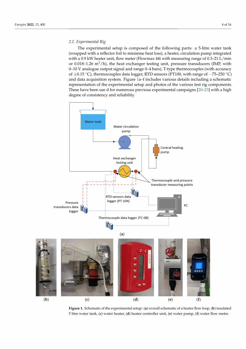
The experimental setup is composed of the following parts: a 5-litre water tank(wrapped with a reflector foil to minimise heat loss), a heater, circulation pump integratedwith a 0.9 kW heater unit, flow meter (Flowmax 44i with measuring range of 0.3–21 L/minor 0.018–1.26 m3/h), the heat exchanger testing unit, pressure transducers (IMP, with0–10 V analogue output signal and range 0–4 bars), T-type thermocouples (with accuracyof ±0.15 ◦C), thermocouples data logger, RTD sensors (PT100, with range of −75–250 ◦C)and data acquisition system. Figure 1a–f includes various details including a schematicrepresentation of the experimental setup and photos of the various test rig components.These have been use d for numerous previous experimental campaigns [20–23] with a highdegree of consistency and reliability.

Energies 2021, 14, x FOR PEER REVIEW 4 of 16

2. Materials and Methods An experimental setup was designed and developed to study the thermal behaviour

of a multi-tube multi-fin heat exchanger. Details of the setup, equipment, instrumentation and uncertainties are given in the following sections.

2.1. Experimental Rig The experimental setup is composed of the following parts: a 5-litre water tank

(wrapped with a reflector foil to minimise heat loss), a heater, circulation pump integrated with a 0.9 kW heater unit, flow meter (Flowmax 44i with measuring range of 0.3–21 L/min or 0.018–1.26 m3/h), the heat exchanger testing unit, pressure transducers (IMP, with 0–10 V analogue output signal and range 0–4 bars), T-type thermocouples (with accuracy of ±0.15 °C), thermocouples data logger, RTD sensors (PT100, with range of −75–250 °C) and data acquisition system. Figure 1a–f includes various details including a schematic repre-sentation of the experimental setup and photos of the various test rig components. These have been use d for numerous previous experimental campaigns [20–23] with a high de-gree of consistency and reliability.

(a)

Energies 2021, 14, x FOR PEER REVIEW 5 of 16

(b) (c) (d) (e) (f)

Figure 1. Schematic of the experimental setup: (a) overall schematic of a heater flow loop, (b) insu-lated 5 litre water tank, (c) water heater, (d) heater controller unit, (e) water pump, (f) water flow meter.

2.1.1. Heat Exchanger Testing Unit Figure 2a illustrates a schematic diagram of the heat exchanger testing unit. The test-

ing unit was made from a 2-mm thick galvanised steel sheet. The dimensions of the unit include a length of 0.650 m; and corresponding width of 0.165 m and a height of 0.175 m. Airflow is supplied to the testing unit using a single-sided centrifugal fan which has an incorporated electric motor. The fan has a power rating of 119 W and is able to deliver a maximum of 610 m3/h airflow rate. The speed of the fan’s electric motor was controlled using a potentiometer.

The incoming flow was conditioned by using a honeycomb structure and various velocity components associated with incoming flow were measure by TFI cobra probe [24] at the entry to the test section. A typical cobra probe has four pressure sensing ports, and these pressure values are used to find the three flow velocity components. At the inlet the flow velocity was measured at 25 points to obtain the average velocity using the ASHRAE standard 41.2 [15,25].

The upstream and downstream air temperatures within the test section were meas-ured at two specific locations. At each of the specific locations seven T-type thermocouples were used. The thermocouples have exposed welded copper/constantan tips to minimise it thermal inertia [15]. There are benefits of using multiple thermocouples at each location. Due to this the accuracy is improved since more samples are available for averaging and automatic averaging can be carried out simultaneously. The arrangement of these ther-mocouples at each specific location is shown in Figure 2c. During the experimentation, the thermocouples repeatability was ensured by taking multiple measurements and individ-ual thermocouples were calibrated using a laboratory grade thermometer. All tempera-tures measured were recorded using a data acquisition system [Pico Technology (Pico-Tech)]. The data from the thermocouples were logged were then averaged.

The inlet and outlet water temperatures in the tubes were measured by PicoTech temperature probes (RTD-PT100). The accuracy of these probes is ±0.03 °C during the test-ing and the repeatability in the measurements was ensured by having multiple measure-ments. Also, the probes were calibrated using a standard thermometer. The water flow rate was measured by using the Flowmax 44i water flowmeter which is an ultrasonic-based volumetric flow meter with a ±2% maximum error of measurement and its repeat-ability is within ±0.5%.

Figure 1. Schematic of the experimental setup: (a) overall schematic of a heater flow loop, (b) insulated5 litre water tank, (c) water heater, (d) heater controller unit, (e) water pump, (f) water flow meter.

Energies 2022, 15, 400 5 of 16

2.1.1. Heat Exchanger Testing Unit

Figure 2a illustrates a schematic diagram of the heat exchanger testing unit. Thetesting unit was made from a 2-mm thick galvanised steel sheet. The dimensions of the unitinclude a length of 0.650 m; and corresponding width of 0.165 m and a height of 0.175 m.Airflow is supplied to the testing unit using a single-sided centrifugal fan which has anincorporated electric motor. The fan has a power rating of 119 W and is able to deliver amaximum of 610 m3/h airflow rate. The speed of the fan’s electric motor was controlledusing a potentiometer.

Energies 2021, 14, x FOR PEER REVIEW 6 of 16

(a)

(b)

(c)

Figure 2. (a) Schematic representation of the heat exchanger testing unit (b) dimensions of the plain fin heat exchanger (c) Arrangement of thermocouples at the specific measurement location.

The heat exchanger’s airside pressure drop was measured using a DPM TT550 micro-manometer. It has the ability of measuring the static pressure within the range: 0.4–5000 Pa. The heat exchanger’s water side pressure drop was measured using two pressure transducers. They were respectively placed at the water inlet and outlet tubes and were

Figure 2. (a) Schematic representation of the heat exchanger testing unit (b) dimensions of the plainfin heat exchanger (c) Arrangement of thermocouples at the specific measurement location.

Energies 2022, 15, 400 6 of 16

The incoming flow was conditioned by using a honeycomb structure and variousvelocity components associated with incoming flow were measure by TFI cobra probe [24]at the entry to the test section. A typical cobra probe has four pressure sensing ports, andthese pressure values are used to find the three flow velocity components. At the inlet theflow velocity was measured at 25 points to obtain the average velocity using the ASHRAEstandard 41.2 [15,25].

The upstream and downstream air temperatures within the test section were measuredat two specific locations. At each of the specific locations seven T-type thermocouples wereused. The thermocouples have exposed welded copper/constantan tips to minimise itthermal inertia [15]. There are benefits of using multiple thermocouples at each location.Due to this the accuracy is improved since more samples are available for averaging andautomatic averaging can be carried out simultaneously. The arrangement of these thermo-couples at each specific location is shown in Figure 2c. During the experimentation, thethermocouples repeatability was ensured by taking multiple measurements and individualthermocouples were calibrated using a laboratory grade thermometer. All temperaturesmeasured were recorded using a data acquisition system [Pico Technology (PicoTech)]. Thedata from the thermocouples were logged were then averaged.

The inlet and outlet water temperatures in the tubes were measured by PicoTechtemperature probes (RTD-PT100). The accuracy of these probes is ±0.03 ◦C during thetesting and the repeatability in the measurements was ensured by having multiple mea-surements. Also, the probes were calibrated using a standard thermometer. The water flowrate was measured by using the Flowmax 44i water flowmeter which is an ultrasonic-basedvolumetric flow meter with a ±2% maximum error of measurement and its repeatability iswithin ±0.5%.

The heat exchanger’s airside pressure drop was measured using a DPM TT550 micro-manometer. It has the ability of measuring the static pressure within the range: 0.4–5000 Pa.The heat exchanger’s water side pressure drop was measured using two pressure trans-ducers. They were respectively placed at the water inlet and outlet tubes and were inturn connected to a PC via a USB-1616HS Series Data Acquisition interface. The voltagereadings were then recorded. Using the calibration equations these voltage values wereconverted to corresponding pressure values.

2.1.2. Fin Geometries

Three main fin geometries were used to carry out this study. They are:

a. Plain finb. Perforated plain finc. Louvred fin

The plain fin heat exchanger used in the present investigation is a multi-tube multi-fintype. There are two tube rows provided, and each tube has a diameter of 9.52 mm. Eachof the rows included five 0.26-mm thick copper tubes and the overall length of each tubeis 0.130 m. The bend of each tube has a diameter of 16 mm. The heat exchanger has21 staggered 0.12 mm aluminium plain fins which have a width of 43.3 mm and a height125.3 mm. Along the heat exchanger, the fins are placed at a distance of 4.23 mm from eachother. The dimensions of the heat exchangers are shown in Figure 2b.

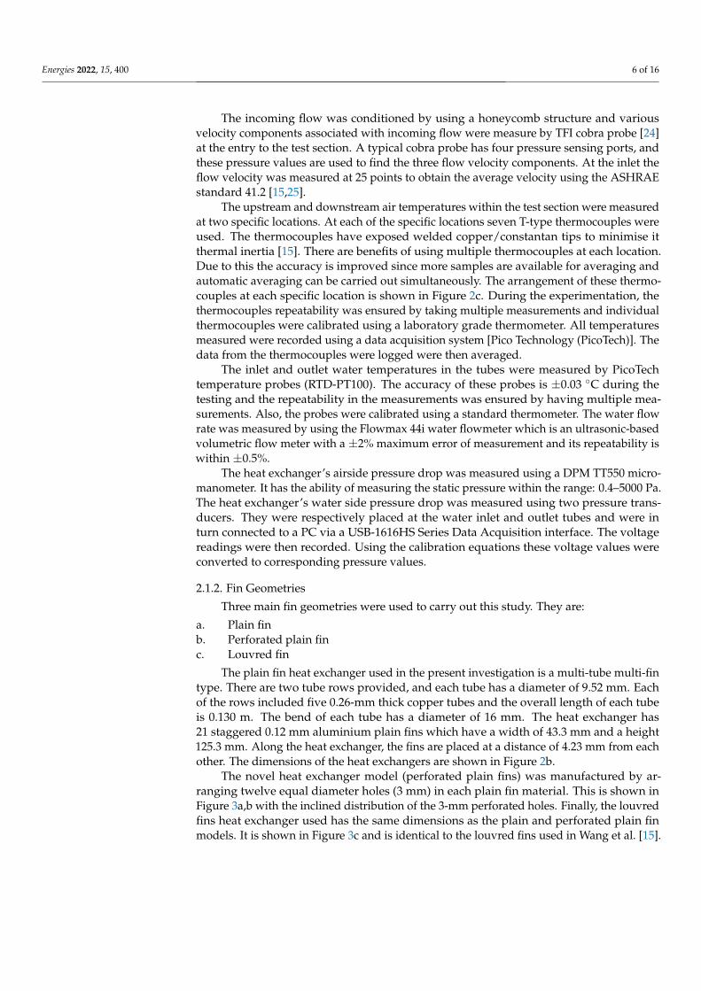
The novel heat exchanger model (perforated plain fins) was manufactured by ar-ranging twelve equal diameter holes (3 mm) in each plain fin material. This is shown inFigure 3a,b with the inclined distribution of the 3-mm perforated holes. Finally, the louvredfins heat exchanger used has the same dimensions as the plain and perforated plain finmodels. It is shown in Figure 3c and is identical to the louvred fins used in Wang et al. [15].

Energies 2022, 15, 400 7 of 16

Energies 2021, 14, x FOR PEER REVIEW 7 of 16

in turn connected to a PC via a USB-1616HS Series Data Acquisition interface. The voltage readings were then recorded. Using the calibration equations these voltage values were converted to corresponding pressure values.

2.1.2. Fin Geometries Three main fin geometries were used to carry out this study. They are:

a. Plain fin b. Perforated plain fin c. Louvred fin

The plain fin heat exchanger used in the present investigation is a multi-tube multi-fin type. There are two tube rows provided, and each tube has a diameter of 9.52 mm. Each of the rows included five 0.26-mm thick copper tubes and the overall length of each tube is 0.130 m. The bend of each tube has a diameter of 16 mm. The heat exchanger has 21 staggered 0.12 mm aluminium plain fins which have a width of 43.3 mm and a height 125.3 mm. Along the heat exchanger, the fins are placed at a distance of 4.23 mm from each other. The dimensions of the heat exchangers are shown in Figure 2b.

The novel heat exchanger model (perforated plain fins) was manufactured by arrang-ing twelve equal diameter holes (3 mm) in each plain fin material. This is shown in Figure 3a,b with the inclined distribution of the 3-mm perforated holes. Finally, the louvred fins heat exchanger used has the same dimensions as the plain and perforated plain fin mod-els. It is shown in Figure 3c and is identical to the louvred fins used in Wang et al. [15].

(a) (b) (c) (d)

Figure 3. (a) Picture of perforated plain fin type heat exchanger, (b) perforated holes’ arrangement, (c) louvred fins heat exchanger, (d) louvred fin shape.

2.1.3. Experimental Procedure Steady-state tests provide thermal performances of the heat exchanger that are time

independent. The test process involved drawing an airflow within the heat exchanger on the fin-side and allowing hot water to circulate through the tubes within the heat ex-changer. Both the average air velocity (from 0.7 m/s to 4 m/s) and water flow rates (0.12 to

Figure 3. (a) Picture of perforated plain fin type heat exchanger, (b) perforated holes’ arrangement,(c) louvred fins heat exchanger, (d) louvred fin shape.

2.1.3. Experimental Procedure

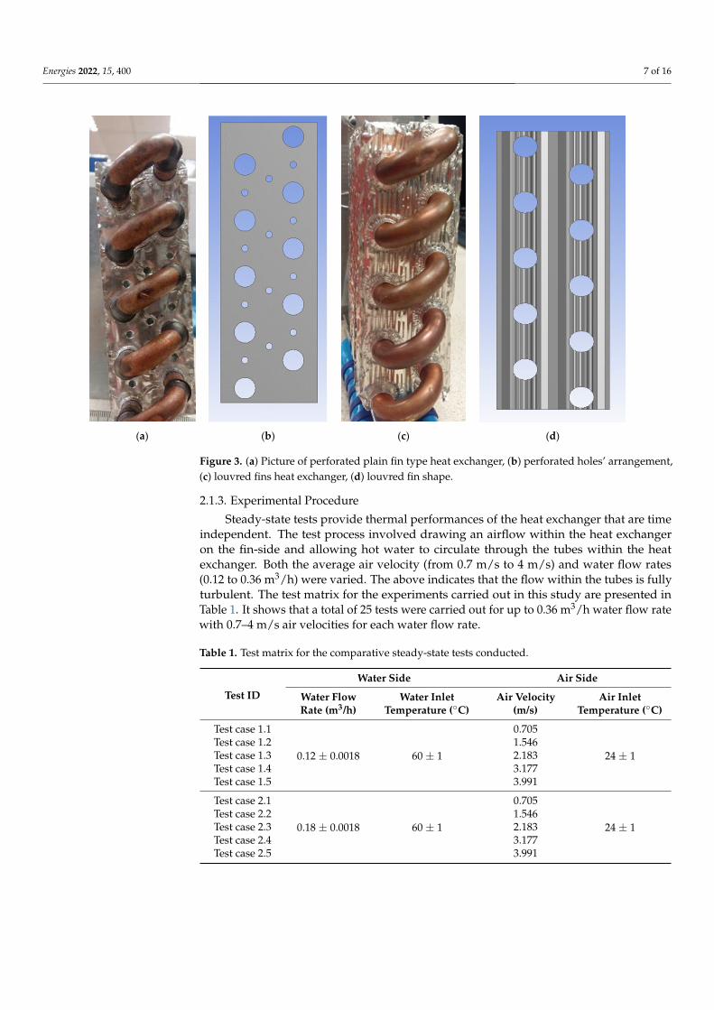
Steady-state tests provide thermal performances of the heat exchanger that are timeindependent. The test process involved drawing an airflow within the heat exchangeron the fin-side and allowing hot water to circulate through the tubes within the heatexchanger. Both the average air velocity (from 0.7 m/s to 4 m/s) and water flow rates(0.12 to 0.36 m3/h) were varied. The above indicates that the flow within the tubes is fullyturbulent. The test matrix for the experiments carried out in this study are presented inTable 1. It shows that a total of 25 tests were carried out for up to 0.36 m3/h water flow ratewith 0.7–4 m/s air velocities for each water flow rate.

Table 1. Test matrix for the comparative steady-state tests conducted.

Test ID

Water Side Air Side

Water FlowRate (m3/h)

Water InletTemperature (◦C)

Air Velocity(m/s)

Air InletTemperature (◦C)

Test case 1.1

0.12 ± 0.0018 60 ± 1

0.705

24 ± 1Test case 1.2 1.546Test case 1.3 2.183Test case 1.4 3.177Test case 1.5 3.991

Test case 2.1

0.18 ± 0.0018 60 ± 1

0.705

24 ± 1Test case 2.2 1.546Test case 2.3 2.183Test case 2.4 3.177Test case 2.5 3.991

Energies 2022, 15, 400 8 of 16

Table 1. Cont.

Test ID

Water Side Air Side

Water FlowRate (m3/h)

Water InletTemperature (◦C)

Air Velocity(m/s)

Air InletTemperature (◦C)

Test case 3.1

0.24 ± 0.0018 60 ± 1

0.705

24 ± 1Test case 3.2 1.546Test case 3.3 2.183Test case 3.4 3.177Test case 3.5 3.991

Test case 4.1

0.3 ± 0.0018 60 ± 1

0.705

24 ± 1Test case 4.2 1.546Test case 4.3 2.183Test case 4.4 3.177Test case 4.5 3.991

Test case 5.1

0.36 ± 0.0018 60 ± 1

0.705

24 ± 1Test case 5.2 1.546Test case 5.3 2.183Test case 5.4 3.177Test case 5.5 3.991

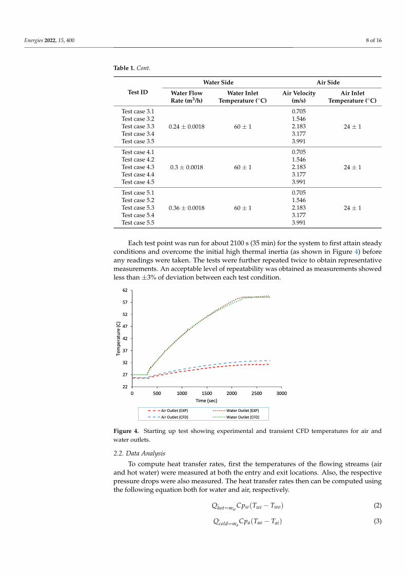
Each test point was run for about 2100 s (35 min) for the system to first attain steadyconditions and overcome the initial high thermal inertia (as shown in Figure 4) beforeany readings were taken. The tests were further repeated twice to obtain representativemeasurements. An acceptable level of repeatability was obtained as measurements showedless than ±3% of deviation between each test condition.

Energies 2021, 14, x FOR PEER REVIEW 8 of 16

0.36 m3/h) were varied. The above indicates that the flow within the tubes is fully turbu-lent. The test matrix for the experiments carried out in this study are presented in Table 1. It shows that a total of 25 tests were carried out for up to 0.36 m3/h water flow rate with 0.7–4 m/s air velocities for each water flow rate.

Each test point was run for about 2100 s (35 min) for the system to first attain steady conditions and overcome the initial high thermal inertia (as shown in Figure 4) before any readings were taken. The tests were further repeated twice to obtain representative meas-urements. An acceptable level of repeatability was obtained as measurements showed less than ±3% of deviation between each test condition.

Figure 4. Starting up test showing experimental and transient CFD temperatures for air and water outlets.

Table 1. Test matrix for the comparative steady-state tests conducted.

Test ID Water Side Air Side

Water Flow Rate (m3/h)

Water Inlet Tem-perature (°C)

Air Velocity (m/s)

Air Inlet Temper-ature (°C)

Test case 1.1

0.12 ± 0.0018 60 ± 1

0.705

24 ± 1 Test case 1.2 1.546 Test case 1.3 2.183 Test case 1.4 3.177 Test case 1.5 3.991 Test case 2.1

0.18 ± 0.0018 60 ± 1

0.705

24 ± 1 Test case 2.2 1.546 Test case 2.3 2.183 Test case 2.4 3.177 Test case 2.5 3.991 Test case 3.1

0.24 ± 0.0018 60 ± 1

0.705

24 ± 1 Test case 3.2 1.546 Test case 3.3 2.183 Test case 3.4 3.177 Test case 3.5 3.991 Test case 4.1

0.3 ± 0.0018 60 ± 1

0.705

24 ± 1 Test case 4.2 1.546 Test case 4.3 2.183 Test case 4.4 3.177

Figure 4. Starting up test showing experimental and transient CFD temperatures for air andwater outlets.

2.2. Data Analysis

To compute heat transfer rates, first the temperatures of the flowing streams (airand hot water) were measured at both the entry and exit locations. Also, the respectivepressure drops were also measured. The heat transfer rates then can be computed usingthe following equation both for water and air, respectively.

Q.hot=m.

wCpw(Twi − Two) (2)

Q.cold=m.

aCpa(Tao − Tai) (3)

Energies 2022, 15, 400 9 of 16

where the subscripts a and w indicate air and water; i and o indicate inlet and outlet,respectively. The average value of the heat transfer rate (

.Qavg) can be computed as follows:

Q.avg =

Q.hot + Q.

cold2

(4)

Furthermore, in order to carry out an assessment of heat transfer and pressure dropcharacteristics, the Colburn factor (j) and Fanning friction factor (f ) were calculated andused for this purpose. The f -factor symbolises the pressure drop characteristics while thej-factor symbolises the heat transfer process and the j/f ratio is termed as the efficiencyindex. The Colburn factor j and the friction factor f are respectively calculated using:

j = StPr2/3 (5)

f =Ac

Ao

ρm

ρ1

[2ρ1∆P

G2c

−(

Kc + 1 − σ2)− 2

(ρ1

ρ2− 1

)+

(1 − σ2 − Ke

)ρ1

ρ2

](6)

where Ac is the minimum free flow area of the air side; Ao is the total surface area ofthe air side; the variables Kc and Ke are the entrance and exit pressure loss coefficients.Equation (6) was developed by Kays and London [21] using the data from Figures 14–26 inMcQuiston et al. [2]. Additionally, the Stanton and the Prandtl numbers used to define theColburn j-factor in Equation (5) are, respectively, given as:

St =ho

ρaVa(max)cpa(7)

Pr =µcpa

λ(8)

where ho is the heat transfer coefficient calculated using the total surface area of the airside; ρa is the density of air, Va(max) is the maximum air velocity; cpa is the specific heatcapacity of air; µ is the air dynamic viscosity and λ is its thermal conductivity. Since thef - and j-factors are most commonly used by researchers to assess the performance of heatexchanger fin strips, they will be used here for assessing the performance of the threegeometries used in this study.

3. Results

In this section, the trend of the measured pressure drops, and heat transfer rates arestudied and discussed in detail. These values were used to calculate the j- and f-factors,and the efficiency index for characterising the performance of the three fin and tube heatexchanger models.

3.1. Performance Comparison of Fin Geometry

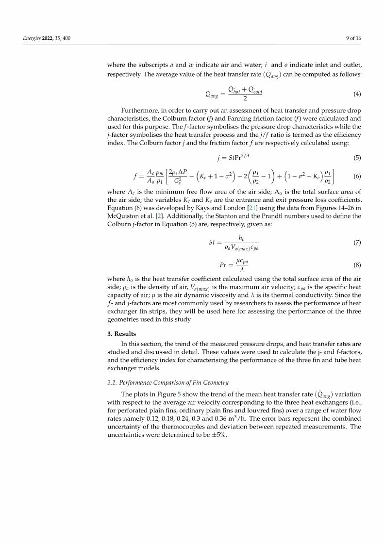
The plots in Figure 5 show the trend of the mean heat transfer rate (.

Qavg) variationwith respect to the average air velocity corresponding to the three heat exchangers (i.e.,for perforated plain fins, ordinary plain fins and louvred fins) over a range of water flowrates namely 0.12, 0.18, 0.24, 0.3 and 0.36 m3/h. The error bars represent the combineduncertainty of the thermocouples and deviation between repeated measurements. Theuncertainties were determined to be ±5%.

Energies 2022, 15, 400 10 of 16

Energies 2021, 14, x FOR PEER REVIEW 10 of 16

3.1. Performance Comparison of Fin Geometry The plots in Figure 5 show the trend of the mean heat transfer rate ( ) variation

with respect to the average air velocity corresponding to the three heat exchangers (i.e., for perforated plain fins, ordinary plain fins and louvred fins) over a range of water flow rates namely 0.12, 0.18, 0.24, 0.3 and 0.36 m3/h. The error bars represent the combined uncertainty of the thermocouples and deviation between repeated measurements. The un-certainties were determined to be ±5%.

(a) (b) (c)

(d) (e)

Figure 5. Variation of ( [W]) against Va for various heat exchangers; (a) for water flow rate 0.12 m3/h, (b) for water flow rate 0.18 m3/h, (c) for water flow rate 0.24 m3/h, (d) for water flow rate 0.3 m3/h and (e) for water flow rate 0.36 m3/h.

Figure 5a shows the variation of average heat transfer rate against the average air velocity for water flow rate of 0.12 m3/h for different heat exchanger geometries. It can be seen from the figure that the louvred fins heat exchanger exhibited a higher mean heat transfer rate when compared with the perforated plain, and plain fin heat exchangers. For all cases, the average heat transfer rate increases as the water flow rate increases, first at a faster rate at lower air velocities and the rate of increase starts to decrease, more noticeably beyond 3 m/s. Figure 5b shows a similar trend but the rate of heat transfer increase beyond 3 m/s is now higher than the previous case and this is maintained for water flow rates of 0.24, 0.3 and 0.36 m3/h as shown in Figure 5c–e, respectively. The louvred fin geometry produced correspondingly higher increase in the average heat transfer rates especially at 0.3 and 0.36 m3/h water flow rates than at the lower water flow rates.

Figure 6a shows the variation of pressure gradient on air side with average air veloc-ity at a given water flow rate. It can be seen that for louvered fins heat exchanger pressured drop increases almost linearly with air velocity. The louvred fin geometry exhibits much higher pressure drops than the other geometries. It is seen from the figure that the lou-vered fin produces up to 380% more pressure drop than the plain fin geometry at = 4

0 1 2 3 4 5Va [m/s]

0

100

200

300

400

500

600

700

Plain finLouvred finPerforated plain fin

0 1 2 3 4 5Va [m/s]

0

100

200

300

400

500

600

700

Plain finLouvred finPerforated plain fin

0 1 2 3 4 5Va [m/s]

0

100

200

300

400

500

600

700

Plain finLouvred finPerforated plain fin

0 1 2 3 4 5Va [m/s]

0

100

200

300

400

500

600

700

Plain finLouvred finPerforated plain fin

0 1 2 3 4 5Va [m/s]

0

100

200

300

400

500

600

700

Plain finLouvred finPerforated plain fin

Figure 5. Variation of (.

Qavg [W]) against Va for various heat exchangers; (a) for water flow rate0.12 m3/h, (b) for water flow rate 0.18 m3/h, (c) for water flow rate 0.24 m3/h, (d) for water flow rate0.3 m3/h and (e) for water flow rate 0.36 m3/h.

Figure 5a shows the variation of average heat transfer rate against the average airvelocity for water flow rate of 0.12 m3/h for different heat exchanger geometries. It canbe seen from the figure that the louvred fins heat exchanger exhibited a higher mean heattransfer rate when compared with the perforated plain, and plain fin heat exchangers. Forall cases, the average heat transfer rate increases as the water flow rate increases, first at afaster rate at lower air velocities and the rate of increase starts to decrease, more noticeablybeyond 3 m/s. Figure 5b shows a similar trend but the rate of heat transfer increase beyond3 m/s is now higher than the previous case and this is maintained for water flow rates of0.24, 0.3 and 0.36 m3/h as shown in Figure 5c–e, respectively. The louvred fin geometryproduced correspondingly higher increase in the average heat transfer rates especially at0.3 and 0.36 m3/h water flow rates than at the lower water flow rates.

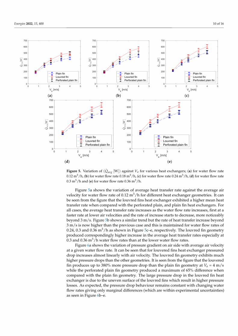
Figure 6a shows the variation of pressure gradient on air side with average air velocityat a given water flow rate. It can be seen that for louvered fins heat exchanger pressureddrop increases almost linearly with air velocity. The louvred fin geometry exhibits muchhigher pressure drops than the other geometries. It is seen from the figure that the louveredfin produces up to 380% more pressure drop than the plain fin geometry at Va = 4 m/swhile the perforated plain fin geometry produced a maximum of 65% difference whencompared with the plain fin geometry. The large pressure drop in the louvred fin heatexchanger is due to the uneven surface of the louvred fins which result in higher pressurelosses. As expected, the pressure drop behaviour remains constant with changing waterflow rates giving only marginal differences (which are within experimental uncertainties)as seen in Figure 6b–e.

Energies 2022, 15, 400 11 of 16

Energies 2021, 14, x FOR PEER REVIEW 11 of 16

m/s while the perforated plain fin geometry produced a maximum of 65% difference when compared with the plain fin geometry. The large pressure drop in the louvred fin heat exchanger is due to the uneven surface of the louvred fins which result in higher pressure losses. As expected, the pressure drop behaviour remains constant with changing water flow rates giving only marginal differences (which are within experimental uncertainties) as seen in Figure 6b–e.

(a) (b) (c)

(d) (e)

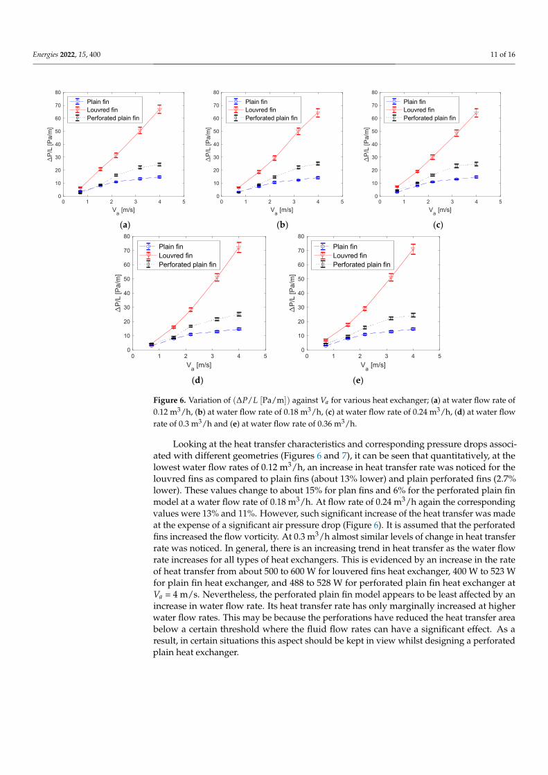
Figure 6. Variation of (∆ / [Pa/m]) against for various heat exchanger; (a) at water flow rate of 0.12 m3/h, (b) at water flow rate of 0.18 m3/h, (c) at water flow rate of 0.24 m3/h, (d) at water flow rate of 0.3 m3/h and (e) at water flow rate of 0.36 m3/h.

Looking at the heat transfer characteristics and corresponding pressure drops asso-ciated with different geometries (Figures 6 and 7), it can be seen that quantitatively, at the lowest water flow rates of 0.12 m3/h, an increase in heat transfer rate was noticed for the louvred fins as compared to plain fins (about 13% lower) and plain perforated fins (2.7% lower). These values change to about 15% for plan fins and 6% for the perforated plain fin model at a water flow rate of 0.18 m3/h. At flow rate of 0.24 m3/h again the corresponding values were 13% and 11%. However, such significant increase of the heat transfer was made at the expense of a significant air pressure drop (Figure 6). It is assumed that the perforated fins increased the flow vorticity. At 0.3 m3/h almost similar levels of change in heat transfer rate was noticed. In general, there is an increasing trend in heat transfer as the water flow rate increases for all types of heat exchangers. This is evidenced by an increase in the rate of heat transfer from about 500 to 600 W for louvered fins heat ex-changer, 400 W to 523 W for plain fin heat exchanger, and 488 to 528 W for perforated plain fin heat exchanger at = 4 m/s. Nevertheless, the perforated plain fin model ap-pears to be least affected by an increase in water flow rate. Its heat transfer rate has only marginally increased at higher water flow rates. This may be because the perforations have reduced the heat transfer area below a certain threshold where the fluid flow rates

0 1 2 3 4 5Va [m/s]

0

10

20

30

40

50

60

70

80

P/L

[Pa/

m]

Plain finLouvred finPerforated plain fin

0 1 2 3 4 5Va [m/s]

0

10

20

30

40

50

60

70

80

P/L

[Pa/

m]

Plain finLouvred finPerforated plain fin

0 1 2 3 4 5Va [m/s]

0

10

20

30

40

50

60

70

80

P/L

[Pa/

m]

Plain finLouvred finPerforated plain fin

0 1 2 3 4 5Va [m/s]

0

10

20

30

40

50

60

70

80

P/L

[Pa/

m]

Plain finLouvred finPerforated plain fin

0 1 2 3 4 5Va [m/s]

0

10

20

30

40

50

60

70

80

P/L

[Pa/

m]

Plain finLouvred finPerforated plain fin

Figure 6. Variation of (∆P/L [Pa/m]) against Va for various heat exchanger; (a) at water flow rate of0.12 m3/h, (b) at water flow rate of 0.18 m3/h, (c) at water flow rate of 0.24 m3/h, (d) at water flowrate of 0.3 m3/h and (e) at water flow rate of 0.36 m3/h.

Looking at the heat transfer characteristics and corresponding pressure drops associ-ated with different geometries (Figures 6 and 7), it can be seen that quantitatively, at thelowest water flow rates of 0.12 m3/h, an increase in heat transfer rate was noticed for thelouvred fins as compared to plain fins (about 13% lower) and plain perforated fins (2.7%lower). These values change to about 15% for plan fins and 6% for the perforated plain finmodel at a water flow rate of 0.18 m3/h. At flow rate of 0.24 m3/h again the correspondingvalues were 13% and 11%. However, such significant increase of the heat transfer was madeat the expense of a significant air pressure drop (Figure 6). It is assumed that the perforatedfins increased the flow vorticity. At 0.3 m3/h almost similar levels of change in heat transferrate was noticed. In general, there is an increasing trend in heat transfer as the water flowrate increases for all types of heat exchangers. This is evidenced by an increase in the rateof heat transfer from about 500 to 600 W for louvered fins heat exchanger, 400 W to 523 Wfor plain fin heat exchanger, and 488 to 528 W for perforated plain fin heat exchanger atVa = 4 m/s. Nevertheless, the perforated plain fin model appears to be least affected by anincrease in water flow rate. Its heat transfer rate has only marginally increased at higherwater flow rates. This may be because the perforations have reduced the heat transfer areabelow a certain threshold where the fluid flow rates can have a significant effect. As aresult, in certain situations this aspect should be kept in view whilst designing a perforatedplain heat exchanger.

Energies 2022, 15, 400 12 of 16

Energies 2021, 14, x FOR PEER REVIEW 12 of 16

can have a significant effect. As a result, in certain situations this aspect should be kept in view whilst designing a perforated plain heat exchanger.

Figure 7a shows the variation of friction factor (f) for the heat exchangers as a func-tion of Reynolds number. It shows that the friction factor decreases with increasing Reyn-olds number and is consistent with previous observations including those in the Moody chart for pipe flows. For each of heat exchanger, there is a steep decreasing slope in the curve between Re = 11,000 and 17,000 before slope of the curve becomes flatter. As is seen in the plots, power law curves were fitted to the three sets of data (louvred, plain and perforated fins). This was done to develop a prediction model for f as a function of . It can be seen that all the heat exchangers show slightly different slopes (power of Reynolds number are −0.129, −0.162 and −0.201). For the j-factor the corresponding values of indices are −0.300, −0.407 and −0.424 for the louvred, plain and perforated plain fin geometries, respectively.

(a) (b)

(c)

Figure 7. Variations of (a) friction f-factor (b) Colburn j-factor and (c) efficiency index j/f for different fin arrangements as a function of Reynolds number.

Figure 7b shows the variation of the Colburn j-factor of the three heat exchangers as a function of Reynolds number. It shows that the Colburn j-factor decreases with increas-ing Reynolds number indicating a higher heat transfer rate at lower Reynolds numbers. The louvred fin heat exchanger gave the highest j values within the range 0.011–0.02 com-pared to 0.005–0.011 and 0.004–0.010 for the perforated and plain fin heat exchangers re-spectively. The fitted power law curves to the three sets of data give prediction models for j as a function of . Similar to the f-factor, for the j-factor, there is a slight decrease in

Figure 7. Variations of (a) friction f-factor (b) Colburn j-factor and (c) efficiency index j/f for differentfin arrangements as a function of Reynolds number.

Figure 7a shows the variation of friction factor (f) for the heat exchangers as a functionof Reynolds number. It shows that the friction factor decreases with increasing Reynoldsnumber and is consistent with previous observations including those in the Moody chartfor pipe flows. For each of heat exchanger, there is a steep decreasing slope in the curvebetween Re = 11,000 and 17,000 before slope of the curve becomes flatter. As is seen in theplots, power law curves were fitted to the three sets of data (louvred, plain and perforatedfins). This was done to develop a prediction model for f as a function of Re. It can be seenthat all the heat exchangers show slightly different slopes (power of Reynolds number are−0.129, −0.162 and −0.201). For the j-factor the corresponding values of indices are −0.300,−0.407 and −0.424 for the louvred, plain and perforated plain fin geometries, respectively.

Figure 7b shows the variation of the Colburn j-factor of the three heat exchangers as afunction of Reynolds number. It shows that the Colburn j-factor decreases with increasingReynolds number indicating a higher heat transfer rate at lower Reynolds numbers. Thelouvred fin heat exchanger gave the highest j values within the range 0.011–0.02 comparedto 0.005–0.011 and 0.004–0.010 for the perforated and plain fin heat exchangers respectively.The fitted power law curves to the three sets of data give prediction models for j as a functionof Re. Similar to the f-factor, for the j-factor, there is a slight decrease in slope from plain toperforated fin to louvred with the coefficients and indices of the equations being 0.2446,0.3946, 0.4119 and −0.3, −0.407 and −0.424, respectively. Figure 7c depicts efficiency index(j/f ) variations corresponding to three different heat exchangers as a function of Reynolds

Energies 2022, 15, 400 13 of 16

number with an inverse relationship existing between the efficiency index and Re. Theplain and perforated models exhibited similar behaviour in j/f magnitudes of 0.022–0.036across the entire Re range studied. However, the louvred fin gave much larger values ofthe efficiency index of between 0.37 and 0.49. While the louvred fin exhibits a far moresuperior efficiency than the other two geometries, the plain and perforated plain fin modelsgave near identical behaviour throughout the experimental range of Re investigated–withboth geometries exhibiting a similar efficiency index across the experimental range. Thenature of the curves in Figure 7a–c clearly establish that the friction, Colburn factors andthe efficiency index asymptotically decrease with the Reynolds number for all the threedifferent heat exchanger models. It can be seen that the Colburn and friction factor valuesare significantly higher for the louvred fins heat exchanger as compared to the plain andperforated plain fin geometries. This observation can be explained based on the highersurface area available for the louvred fin heat exchanger as compared to the plain andperforated plain fin heat exchangers. Due to this the heat transfer coefficient for louveredheat exchanger is higher which in turn leads to high Colburn j-factor values.

Based on the heat transfer measurements it can be shown that there is an improvementin the average heat transfer rate (

.Qavg) of nearly 10% and 20% for the perforated plain fin

and louvred fin heat exchangers, respectively, when compared to the plain fin geometry.However, this improvement was accompanied by large increases in the correspondingpressure drop on the airside respectively as earlier highlighted. The data collected duringthe current experiments and after processing were used for the development of the twonew design correlations for predicting the Fanning f- and Colburn j-factors as functions ofthe flow velocity and area available. To represent these in non-dimensional form, Reynoldsnumber and an area ratio term (the ratio of the heat exchanger’s fin surface area divided bythe total surface area) have been used in the correlations.

3.2. Development of New Empirical Relations for Fanning f and Colburn j-Factor

For the complex geometries used in the present investigation, the experimental dataobtained in the present investigation were used for developing a set of novel designequations for the prediction of Fanning f- and the Colburn j-factors. As previously stated,the f - and j-factors quantify the pressure drop and heat transfer characteristics of the heatexchanger units. Therefore, it is imperative to develop correlations that relate them with theflow, fluid, and geometrical parameters. The correlation was developed using multivariateregression analysis using the curve fitting tools in Microsoft Excel’s Solver® which arebased on the least squares’ method. The dimensionless parameters used to develop thepredictive correlation are, as mentioned earlier, the Reynolds number, ReD and the ratiobetween total fin surface area to the total heat transfer surface area

(A f /At

)of the heat

exchanger which is a design parameter used by Palmer et al. [26] that can be used forestimating heat transfer areas needed for a given amount of heat to be transmitted. Otherauthors have used similar dimensionless groupings to correlate the heat transfer propertiesof fin and tube heat exchangers [13,17,18]. The newly derived equations are as follows:

j = 104.595( A f

At

)29.918

ReD−0.374 (9)

f = 101.203( A f

At

)12.811

ReD−0.139 (10)

where ReD is the Reynolds number calculated using the hydraulic diameter of the heatexchanger face’s cross-section; Dc is the outside diameter of the fin’s collar (m): A f is thetotal surface area of the fins (m2); At is the heat exchanger’s overall heat transfer surfacearea (m2). The Equations (9) and (10) show that the Colburn and Fanning factors areinversely proportional to the Reynolds numbers which are consistent with experimentalobservations (in Figure 7a,b). Additionally, the relatively large indices (29.218 and 12.811)

Energies 2022, 15, 400 14 of 16

for the(

A f /At

)parameter reflects the small magnitude of the

(A f /At

)ratio. It is advised

that the equations are valid within the Reynolds number range: 6 × 103 ≤ ReD ≤ 30 × 103

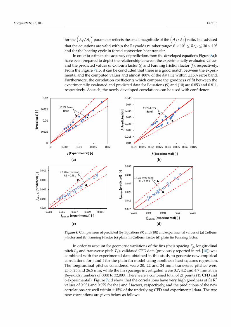
and for the heating cycle in forced convection heat transfer.In order to estimate the accuracy of predictions from the developed equations Figure 8a,b

have been prepared to depict the relationship between the experimentally evaluated valuesand the predicted values of Colburn factor (j) and Fanning friction factor (f ), respectively.From the Figure 7a,b, it can be concluded that there is a good match between the experi-mental and the computed values and almost 100% of the data lie within ±15% error band.Furthermore, the correlation coefficients which compare the goodness of fit between theexperimentally evaluated and predicted data for Equations (9) and (10) are 0.853 and 0.811,respectively. As such, the newly developed correlations can be used with confidence.

Energies 2021, 14, x FOR PEER REVIEW 14 of 16

area (m2). The Equations (9) and (10) show that the Colburn and Fanning factors are in-versely proportional to the Reynolds numbers which are consistent with experimental ob-servations (in Figure 7a,b). Additionally, the relatively large indices (29.218 and 12.811) for the / parameter reflects the small magnitude of the / ratio. It is advised that the equations are valid within the Reynolds number range: 6 1030 10 and for the heating cycle in forced convection heat transfer.

In order to estimate the accuracy of predictions from the developed equations Figure 8a,b have been prepared to depict the relationship between the experimentally evaluated values and the predicted values of Colburn factor (j) and Fanning friction factor (f), re-spectively. From the Figure 7a,b, it can be concluded that there is a good match between the experimental and the computed values and almost 100% of the data lie within ±15% error band. Furthermore, the correlation coefficients which compare the goodness of fit between the experimentally evaluated and predicted data for Equations (9) and (10) are 0.853 and 0.811, respectively. As such, the newly developed correlations can be used with confidence.

(a) (b)

(c) (d)

Figure 8. Comparisons of predicted (by Equations (9) and (10)) and experimental values of (a) Col-burn j-factor and (b) Fanning f-factor (c) plain fin Colburn factor (d) plain fin Fanning factor.

In order to account for geometric variations of the fins (their spacing , longitudinal pitch and transverse pitch ), validated CFD data (previously reported in ref. [18]) was combined with the experimental data obtained in this study to generate new empiri-cal correlations for j and f for the plain fin model using nonlinear least squares regression. The longitudinal pitches considered were 20, 22 and 24 mm; transverse pitches were 23.5, 25 and 26.5 mm; while the fin spacings investigated were 3.7, 4.2 and 4.7 mm at air Reyn-olds numbers of 6000 to 32000. There were a combined total of 21 points (15 CFD and 6 experimental). Figure 7c,d show that the correlations have very high goodness of fit R2

0.003

0.005

0.007

0.009

0.011

0.003 0.005 0.007 0.009 0.011

j plai

n fin

(pre

dict

ed) [

-]

jplain fin (experimental) [-]

± 15% error band; R2 = 0.981

0.015

0.019

0.023

0.027

0.031

0.035

0.015 0.02 0.025 0.03 0.035

f plai

n fin

(pre

dict

ed)

[-]

fplain fin (experimental) [-]

± 15% error band; R2 = 0.979

Figure 8. Comparisons of predicted (by Equations (9) and (10)) and experimental values of (a) Colburnj-factor and (b) Fanning f-factor (c) plain fin Colburn factor (d) plain fin Fanning factor.

In order to account for geometric variations of the fins (their spacing Fp, longitudinalpitch Lp and transverse pitch Tp), validated CFD data (previously reported in ref. [18]) wascombined with the experimental data obtained in this study to generate new empiricalcorrelations for j and f for the plain fin model using nonlinear least squares regression.The longitudinal pitches considered were 20, 22 and 24 mm; transverse pitches were23.5, 25 and 26.5 mm; while the fin spacings investigated were 3.7, 4.2 and 4.7 mm at airReynolds numbers of 6000 to 32,000. There were a combined total of 21 points (15 CFD and6 experimental). Figure 7c,d show that the correlations have very high goodness of fit R2

values of 0.931 and 0.979 for the j and f factors, respectively, and the predictions of the newcorrelations are well within ±15% of the underlying CFD and experimental data. The twonew correlations are given below as follows:

Energies 2022, 15, 400 15 of 16

j = 0.173 ReD−0.388

(Fp

Dc

)−0.199( Lp

Fw

)−0.297( Tp

FH

)−0.089(11)

f = 0.084 ReD−0.213

(Fp

Dc

)−0.334( Lp

Fw

)−0.151( Tp

FH

)−0.262(12)

To summarise, it can be concluded that the developed equations are very much capableof predicting the Fanning f- and Colburn j-factors of these heat exchangers having the statedfin geometries with sufficient accuracy. Consequently, the equations can be used during thedesign and evaluation of existing multi-tube multi-fin heat exchanger with plain, perforatedor louvred fins.

4. Conclusions

This study has presented novel geometric configurations for multi-tube multi-fin heatexchanger. The configurations were designed in order to conduct a robust experimentalinvestigation with three heat exchanger geometries namely plain, perforated plain andlouvred fin heat exchangers. Some important observations were made during the experi-ments and analysis of the pressure drop and heat transfer data. It was found that for allinlet air and water flow rates and hence velocities, the louvred fins produced the highestheat transfer rate. This was attributed to increased surface area available for heat transfer.Conversely, it also produced the highest pressure losses when compared to the other twodesigns. Also, while the new perforated design produced a slightly higher pressure dropthan the plain fin design, due to the vortices generated by the perforations, an enhance-ment in its heat transfer characteristics was observed when comparing with the plain andlouvred fin models. This enhancement is relatively high at a small water flow rate. Theexperimental results were subsequently used to generate a set of novel empirical equationsfor design optimisation which can be used to predict the heat transfer and pressure dropcharacteristics of the heat exchangers represented by the Colburn and Fanning factors.The empirical equations were developed as functions of the heat exchangers’ geometricalparameters, and we have shown that the performance of the equations are well withinacceptable ±15% error margins in relation to the experimental data.

Author Contributions: M.A.: Experimentation, Data curation, formal analysis, Investigation, method-ology, validation, visualization, writing—original draft; R.M.: Conceptualisation, supervision,writing—review and editing; A.M.A.: Writing—review & editing, formal analysis; K.J.K.: supervision,formal analysis, writing—review and editing. All authors have read and agreed to the publishedversion of the manuscript.

Funding: This research did not receive any external funding.

Data Availability Statement: Data is available upon reasonable request.

Conflicts of Interest: The authors declare no conflict of interest.

References1. Shah, R.K.; Sekulic, D.P. Fundamentals of Heat Exchanger Design; John Wiley & Sons: Hoboken, NJ, USA, 2003.2. Mcquiston, F.C.; Parker, J.D.; Spilter, J.K. Heating, Ventilating, and Air Conditioning: Analysis and Design; Wiley: Hoboken, NJ,

USA, 2004.3. Naphon, P.; Wongwises, S. A review of flow and heat transfer characteristics in curved tubes. Renew. Sustain. Energy Rev. 2006, 10,

463–490. [CrossRef]4. Thulukkanam, K. Heat Exchanger Design Handbook, 2nd ed.; Taylor & Francis: Abingdon, UK, 2013.5. Wilson, E.E. A basis for rational design of heat transfer apparatus. J. Am. Soc. Mech. Eng. 1915, 37, 546–551.6. Sieder, E.N.; Corporation, G.E.T.A.T.E.F.W.; York, N. Heat Transfer and Pressure Drop of Liquids in Tubes O Oil A, Heating Oil B,

Heating Oil A, Cooling Oil C, Cooling; American Chemical Society: New York, NY, USA, 2021.7. Colburn, A.P. A method of correlating forced convection heat-transfer data and a comparison with fluid friction. Int. J. Heat Mass

Transf. 1964, 7, 1359–1384. [CrossRef]8. Dittus, F.W.; Boelter, L.M.K. Heat transfer in automobile radiators of the tubular type. Int. Commun. Heat Mass Transf. 1985, 12,

3–22. [CrossRef]

Energies 2022, 15, 400 16 of 16

9. Wang, C.-C.; Chang, Y.-J.; Hsieh, Y.-C.; Lin, Y.-T. Sensible heat and friction characteristics of plate fin-and-tube heat exchangershaving plane fins. Int. J. Refrig. 1996, 19, 223–230. [CrossRef]

10. Abu Madi, M.; Johns, R.; Heikal, M. Performance characteristics correlation for round tube and plate finned heat exchangers. Int.J. Refrig. 1998, 21, 507–517. [CrossRef]

11. Webb, R.; Kim, N.-H. Advances in Air-Cooled Heat Exchanger Technology. J. Enhanc. Heat Transf. 2007, 14, 1–26. [CrossRef]12. Wang, C.-C. A survey of recent patents of fin-and-tube heat exchangers from 2001 to 2009. Int. J. Air-Cond. Refrig. 2010, 18, 1–13.

[CrossRef]13. Wang, C.-C.; Lee, W.-S.; Sheu, W.-J. A comparative study of compact enhanced fin-and-tube heat exchangers. Int. J. Heat Mass

Transf. 2001, 44, 3565–3573. [CrossRef]14. Fernández-Seara, J.; Uhía, F.J.; Sieres, J.; Campo, A. A general review of the Wilson plot method and its modifications to determine

convection coefficients in heat exchange devices. Appl. Therm. Eng. 2007, 27, 2745–2757. [CrossRef]15. Wang, C.-C.; Chen, K.-Y.; Liaw, J.-S.; Tseng, C.-Y. An experimental study of the air-side performance of fin-and-tube heat

exchangers having plain, louver, and semi-dimple vortex generator configuration. Int. J. Heat Mass Transf. 2015, 80, 281–287.[CrossRef]

16. Liu, X.; Yu, J.; Yan, G. A numerical study on the air-side heat transfer of perforated finned-tube heat exchangers with large finpitches. Int. J. Heat Mass Transf. 2016, 100, 199–207. [CrossRef]

17. Kalantari, H.; Ghoreishi-Madiseh, S.A.; Kurnia, J.C.; Sasmito, A.P. An analytical correlation for conjugate heat transfer in fin andtube heat exchangers. Int. J. Therm. Sci. 2021, 164, 106915. [CrossRef]

18. Altwieb, M.; Kubiak, K.J.; Aliyu, A.M.; Mishra, R. A new three-dimensional CFD model for efficiency optimisation of fluid-to-airmulti-fin heat exchanger. Therm. Sci. Eng. Prog. 2020, 19, 100658. [CrossRef]

19. Altwieb, M.O.; Mishra, R. Experimental and Numerical Investigations on the Response of a Multi Tubes and Fins Heat Exchangerunder Steady State Operating Conditions. In Proceedings of the 6th International and 43rd National Conference on FluidMechanics and Fluid Power, Allahabad, India, 15–17 December 2016; pp. 1–3.

20. Singh, D.; Aliyu, A.; Charlton, M.; Mishra, R.; Asim, T.; Oliveira, A. Local multiphase flow characteristics of a severe-servicecontrol valve. J. Pet. Sci. Eng. 2020, 195, 107557. [CrossRef]

21. Singh, D.; Charlton, M.; Asim, T.; Mishra, R.; Townsend, A.; Blunt, L. Quantification of additive manufacturing induced variationsin the global and local performance characteristics of a complex multi-stage control valve trim. J. Pet. Sci. Eng. 2020, 190, 107053.[CrossRef]

22. Asim, T.; Mishra, R.; Oliveira, A.; Charlton, M. Effects of the geometrical features of flow paths on the flow capacity of a controlvalve trim. J. Pet. Sci. Eng. 2019, 172, 124–138. [CrossRef]

23. Asim, T.; Charlton, M.; Mishra, R. CFD based investigations for the design of severe service control valves used in energy systems.Energy Convers. Manag. 2017, 153, 288–303. [CrossRef]

24. TFI. Cobra Probe. 2021. Available online: https://www.turbulentflow.com.au/Products/CobraProbe/CobraProbe.php (accessedon 6 December 2021).

25. ASHRAE. HVAC Design Manual for Hospitals and Clinics; ASHRAE: Atlanta, GA, USA, 2013.26. Palmer, E.; Mishra, R.; Fieldhouse, J. An optimization study of a multiple-row pin-vented brake disc to promote brake cooling

using computational fluid dynamics. Proc. Inst. Mech. Eng. Part D J. Automob. Eng. 2009, 223, 865–875. [CrossRef]