1366 IEEE TRANSACTIONS ON BIOMEDICAL ENGINEERING, VOL. 57, NO. 6, JUNE 2010

Heart Rate Variability on 7-Day Holter MonitoringUsing a Bootstrap Rhythmometric Procedure

Rebeca Goya-Esteban, Inmaculada Mora-Jimenez, Jose Luis Rojo-Alvarez∗, Member, IEEE, Oscar Barquero-Perez,Francisco J. Pastor-Perez, Sergio Manzano-Fernandez, Domingo A. Pascual-Figal, and Arcadi Garcıa-Alberola

Abstract—Heart rate variability (HRV) markers have beenwidely used to characterize the autonomous regulation state ofthe heart from 24-h Holter monitoring, but long-term evolutionof HRV indexes is mostly unknown. A dataset of 7-day Holterrecordings of 22 patients with congestive heart failure was stud-ied. A rhythmometric procedure was designed to characterize theinfradian, circadian, and ultradian components for each patient,as well as circadian and ultradian fluctuations. Furthermore, abootstrap test yielded automatically the rhythmometric model foreach patient. We analyzed the temporal evolution of relevant time-domain (AVNN, SDNN, and NN50), frequency-domain (LF, HF,HFn, and LF/HF), and nonlinear (α1 and SampEn) HRV indexes.Circadian components were the most significant for all HRV in-dexes, but the infradian ones were also strongly present in NN50,HFn, LF/HF, α1 , and SampEn indexes. Among ultradian com-ponents that one corresponding to 12 h, was the most relevant.Long-term monitoring of HRV conveys new potentially relevantrhythmometric information, which can be analyzed by using theproposed automatic procedure.

Index Terms—Bootstrap test, circadian, heart rate variabil-ity (HRV), infradian, long-term monitoring, seven-day Holter,ultradian.

I. INTRODUCTION

LONG-TERM monitoring for cardiac signals is receivingspecial attention. Several studies have shown that home

monitoring can reduce significantly the number of hospital read-missions in congestive heart failure (CHF) patients [1], [2]. Fur-thermore, long-term monitoring systems allow a better treatmentand management of CHF patients [3]. Benefits of long-termmonitoring are being studied also in clinical applications, suchas detection of recurrences after ablation for atrial fibrillation(AF) or analysis of atrial recordings in patients with pacemakerincorporating Holter functionality [4], [5]. Seven-day ambula-

Manuscript received August 1, 2009; revised November 13, 2009 and January7, 2010; accepted January 7, 2010. Date of publication February 17, 2010; date ofcurrent version May 14, 2010. This work was supported in part by the ResearchProject from Medtronic Iberica SA, and in part by the Spanish Governmentunder the Research Projects URJC-CM-2008-CET-3732 and TEC2007-68096-C02TCM. Asterisk indicates corresponding author.

R. Goya-Esteban, I. Mora-Jimenez, and O. Barquero-Perez are with the De-partment of Signal Theory and Communications, University Rey Juan Carlos,Fuenlabrada-28943, Madrid, Spain (e-mail: rebeca.goyaesteban@urjc.es;inmaculada.mora@urjc.es; oscar.barquero@urjc.es).

∗J. L. Rojo-Alvarez is with the Department of Signal Theory and Communica-tions, University Rey Juan Carlos, Fuenlabrada-28943, Madrid, Spain (e-mail:joseluis.rojo@urjc.es).

F. J. Pastor-Perez, S. Manzano-Fernandez, D. A. Pascual-Figal, andA. Garcıa-Alberola are with the Arrhythmia Unit, Hospital Virgen de laArrixaca of Murcia, 30120 Murcia, Spain (e-mail: franpastor79@hotmail.com;sergiosmf13@hotmail.com; dapascual@servicam.com).

Color versions of one or more of the figures in this paper are available onlineat http://ieeexplore.ieee.org.

Digital Object Identifier 10.1109/TBME.2010.2040899

tory ECG monitoring, following acute stroke or transient is-chemic attack, has identified patients with AF, which were notdetected with 24-h ECG recordings [6]. Therefore, the clinicalusefulness and meaning of well-known clinical cardiac indexesis likely to be reanalyzed in the long-term monitoring settingduring the next years.

Heart rate variability (HRV) is a relevant marker of the auto-nomic nervous system (ANS) control on the heart. This markerhas been proposed for risk stratification of lethal arrhythmiasafter acute myocardial infarction, as well as for prognosis ofsudden death events [7]–[9]. Though a number of studies havetried to prove the clinical utility of HRV as a marker of theautonomic activity, there are few studies about the clinical in-formation provided by HRV markers in long-term recordings(longer than 24 h). Regarding rhythmometric patterns of HRVindexes, the circadian rhythm has been well characterized inhealthy and pathological subjects [10], [11]. The HRV ultra-dian rhythms (components at frequencies higher than that cor-responding to a period of about 24 h) have also been studied to alesser extent [12]. However, to our best knowledge, there are fewstudies on infradian cycles of HRV (components at frequencieslower than that corresponding to 24-h period), and they are notpopulational studies [13], [14].

We propose a new rhythmometric tool for analyzing long-term recordings, characterizing not only the circadian patternsof HRV markers, but also infradian and ultradian components,as well as potential narrow-band fluctuations. Our method leanson a bootstrap hypothesis test to construct a rhythmometricmodel by automatically selecting the most relevant spectralcomponents. This approach is applied to analyze some of themost relevant HRV markers of different nature (time-domain,frequency-domain, and nonlinear indexes) [8] in a long-termscenario beyond 24 h. In particular, we collected and analyzed adatabase of CHF patients 7-day Holters due to the special clin-ical relevance that long-term monitoring has on CHF patients.

The structure of the paper is as follows. Section II brieflysummarizes the precedents on HRV and rhythmometric analy-sis. In Section III, the proposed automatic rhythmometric anal-ysis method is introduced. In Section IV, the CHF databaseis analyzed with our procedure, and the rhythmometric modelcorresponding to each HRV index is studied, both in time andfrequency domains. Finally, Section V contains the discussionand conclusions of our work.

II. BACKGROUND

Traditionally, the occurrence of cardiac arrhythmia, suddencardiac death, and other cardiac events, were thought to be

0018-9294/$26.00 © 2010 IEEE

GOYA-ESTEBAN et al.: HEART RATE VARIABILITY ON 7-DAY HOLTER MONITORING USING BOOTSTRAP 1367

independent of the time of the day. However, in the last decades,the application of rhythmometric analysis procedures to a num-ber of cardiac measurements has shown that many cardiovas-cular events exhibit a pronounced circadian rhythm, indicatingthat the mechanisms for cardiovascular events involve both en-dogenous and exogenous factors [15]. The physiological circa-dian patterns have been shown to be present in blood pressurevariability [16], [17], cardiac arrhythmias [18], drug deliveryand chronotherapeutics [19], and HRV [10], [20], [21], amongothers.

In this paper, we focus on HRV, which reflects variationsin the heart rhythm. The signal used to study HRV is the NNinterval series, defined as the distance between R-waves of con-secutive beats, excluding the ectopic beats. Since HRV yieldsinformation about the ANS, it allows noninvasive assessment ofits state [8]. To study HRV, a number of indexes have been pro-posed in the literature, which can be roughly divided into threefamilies, namely time domain, spectral domain, and nonlinearmethods.

Chronologically, the first methods applied to the HRV analy-sis were the time-domain methods [22]. They generally involvethe calculation of the standard deviation of either the NN in-tervals series, or its first difference. Some of the main temporalindexes are the average of NN intervals (AVNN), the standarddeviation of NN intervals (SDNN), the standard deviation ofthe averages of NN intervals in all 5-min segments of the entirerecording (SDANN), the root mean square of the differencesbetween adjacent NN intervals (RMSSD), and the number ofpairs of adjacent NN intervals differing by more than 50 ms(NN50) [8].

Spectral methods indicate how the power of the signal is dis-tributed as a function of the frequency f . Four spectral bandsare mainly distinguished in the power spectral density of the NNseries, namely high frequency (HF) band with f ∈ [0.15, 0.4]Hz, low frequency (LF) band with f ∈ [0.04, 0.15] Hz, verylow frequency (VLF) band with f ∈ [0.003, 0.04] Hz, and ultralow frequency (ULF) band with f < 0.003 Hz [23]. The corre-sponding spectral indexes (HF, LF, VLF, and ULF) are com-puted according to the power in each band. Normalized spec-tral indexes are also often used, yielding LFn = LF/(LF + HF)for the LF band, HFn = HF/(LF + HF) for the HF band, andLF/HF for the ratio between LF and HF spectral indexes [8].Many studies propose that in normal subjects, an increase inparasympathetic activity is related to a power increase in theHF band. Some authors consider the power in the LF band asa marker of the sympathetic modulation, while for others itincludes both sympathetic and vagal influences [8], [24]. How-ever, in CHF patients, an increase in parasympathetic activitydoes not entail an increase in HF power. Also, some studiesshow that the LF component is virtually abolished in severeheart failure [25]. Regarding the VLF band, it has been shownthat contributions from parasympathetic activity dominate thiscomponent [26]. The physiological meaning of the ULF bandhas not been completely established yet [8].

Nonlinear methods rely on the idea that fluctuations in theNN series may reveal characteristics from complex dynamic sys-tems. Under this assumption, healthy states would correspond to

more complex patterns than pathological states [27]–[29]. Cir-cadian patterns of HRV have been mainly conducted on the ba-sis of time- and frequency-domain methods, however, nonlinearindexes have not been analyzed in this setting. Circadian varia-tions in HRV reflect the changing sympathetic–parasympatheticbalance in the ANS control of the cardiac cycle [15]. Ultradianrhythms have also been found in cardiac autonomic modula-tion [12] and infradian rhythms, such as circaseptan (about sevendays) or circasemiseptan (about 3.5 days) rhythms have beenfound for blood pressure and myocardial infarction [30], [31].

In recent years, long-term monitoring using 7-day Holter hasbeen available, allowing the study of HRV infradian rhythmsand a more consistent estimation of the circadian character-istics. Hence, for analyzing the HRV long-term behavior, weselected representative subsets of indexes from each family ac-cording to their widespread use in the literature. AVNN, SDNN,and NN50, were chosen as time-domain indexes. We used LF,HF, HFn, and LF/HF as representative spectral indexes. Fi-nally, two nonlinear indexes were selected: first, the scalingexponent α1 from detrended fluctuations analysis [32], whichassess the short-term fractal correlation properties (between 3and 16 beats) of the NN series; and second, the sample entropy(SampEn) [33], which quantifies the irregularity of a time seriesfrom information theory principles.

III. BOOTSTRAP RHYTHMOMETRIC METHOD

In this section, we present the rhythmometric model to be usedin the analysis of 7-day recordings, giving a rationale for the in-clusion of each kind of spectral component. We also propose anautomatic method to select the relevant components, based onthe estimation of the error distribution between a rhythmometricmodel and the real signal through a paired bootstrap hypothe-sis test. We illustrate the rhythmometric procedure using somesimple synthetic examples.

A. Rhythmometric Model

A number of works (see [34] and references therein) havestudied the circadian variation of a biological parameter ythrough a temporal regression model, named cosinor model andgiven by

y = M + A0 cos(2πf0t + φ0) + e (1)

where the model parameters are: M is the rhythm-adjusted meanor mesor, A0 is the fitted cosine amplitude, f0 is the fundamentalfrequency, which is set by the analyst on the basis of empiricalphysiological information and usually considered as 24 h, andφ0 is the acrophase, which is the lag from a defined referencetimepoint to the crest time in the cosine curve fitted to the data.Term e is a random variable named residual, corresponding tothe difference between actual value y and the value providedby the regression model. In our context, random variable ycorresponds to the HRV index to be analyzed. To determine theregression parameters, we apply the least squares (LS) approachto a physiological time series given by a set S of N pairs ofvalues S = {ti , yi}N

i=1 .

1368 IEEE TRANSACTIONS ON BIOMEDICAL ENGINEERING, VOL. 57, NO. 6, JUNE 2010

In this paper, we extend the regression model in (1) to beable to model both ultradian and infradian rhythms, as well asmoderate fluctuations around the main rhythms. For the sakeof simplicity, we have just considered narrow-band fluctuationscorresponding to the maximum spectral resolution. Regardinginfradian rhythms, which are characterized by a frequency lowerthan that corresponding to the circadian rhythm (f0), we takethem into account by considering additional sinusoidal terms inthe form ij = Aj cos(2πfi

j t + φij ). Assuming that fs is the sam-

pling frequency of the N real data in S, and defining the max-imum spectral resolution available as ∆f = fs/N , infradianfrequencies fi

j are obtained as fij = j∆f , for j = 1, . . . , jmax .

To distinguish moderate fluctuations of fundamental frequencyf0 from the maximum infradian frequency, we limit the last oneto the highest integer multiple of ∆f , which is lower or equalthan f0 − 2∆f , and therefore, jmax = [f0/∆f ] − 2. Collectingall the potential infradian components, we define the term

I =jm a x∑j=1

ij =jm a x∑j=1

Aj cos(2πj∆ft + φij ). (2)

Ultradian rhythms are those whose regular recurrence is incycles of less than 24 h, i.e., they are characterized by a fre-quency higher than f0 . To take them into account, we con-sider again additional sinusoidal terms in (1), now in the formuk = Ak cos(2πfu

k t + φk ), where fuk is a harmonic of the fun-

damental frequency f0 . Thus, fuk can be expressed as fu

k = kf0 ,with k being a natural number from k = 2 (12 h) to k = kmax ,and the ultradian rhythms can be collected in the following term:

U =km a x∑k=2

uk =km a x∑k=2

Ak cos(2πkf0t + φk ). (3)

In particular, for the experimental work in this paper, we consid-ered up to five harmonic components, i.e., kmax = 6, the highestfrequency component corresponding to 4 h cycle.

Finally, we complete the rhythmometric regression model bytaking into account potential narrow-band fluctuations of thecircadian and ultradian rhythms. For this purpose, we includetwo fluctuation terms, denoted as F−

k and F+k , corresponding to

sinusoidal waveforms deviating from the frequency associatedwith the corresponding rhythm, a value given by the maximumspectral resolution, i.e.,

F−k = A−

k cos(2π(fuk − ∆f)t + φ−

k ) (4)

F+k = A+

k cos(2π(fuk + ∆f)t + φ+

k ) (5)

for k = 1 (circadian rhythm) and k = 2, 3, . . . , kmax (ultradianrhythms). Note that fluctuations are not considered for infradiancomponents. Since in this study, we were specially interestedin infradian components, we studied all the possible infradianspectral components multiple of ∆f , hence, (2) comprises all thepossible spectral components from the frequency correspondingto seven days to approximately f0 − 2∆f in steps of ∆f , whichis the maximum spectral resolution.

Taking into account the infradian, circadian, and ultradianrhythms, as well as the narrow-band fluctuations, the proposed

rhythmometric model results in the following expression:

y = M + A0 cos(2πf0t + φ0) + I + U

+km a x∑k=1

(F−

k + F+k

)+ e. (6)

B. Paired Bootstrap Test

The LS method is used to find the regression parameters in(6). To deal with the potential uncertainty in the time series,the spectral components of (6) with little statistical significanceshould be removed. For this purpose, we propose to construct thefinal rhythmometric model from a very simple regression model,just composed of the mesor component (given by parameterM ), and applying an iterative constructive method. This methoditeratively adds to the previous regression model, the sinusoidalcomponent of (6) with the highest mean power, this is at everyiteration, we compare two regression models, so called modelA and model B, where model B is constructed by adding tomodel A, the sinusoidal component of (6) with the highest meanpower.

This model comparison is performed using a paired boot-strap hypothesis test [35]. Specifically, the mean square error(MSE) between the signal provided by model A and the origi-nal signal (EA ) is computed, and also the MSE correspondingto model B (EB ). To test the relevance of the addition of everysinusoidal component, a number of B random resamplings withreplacement of the differences between EA and EB are con-ducted, obtaining ∆E∗(b) = E∗

A (b) − E∗B (b) for each resam-

pling b = 1, . . . , B, where ∗ denotes quantities obtained fromresampling, as usual in bootstrap literature. We fixed B = 2500in all of our experiments.

A suitable statistical hypothesis test is to contrast the nullhypothesis that models A and B have the same unexplainedvariance (H0 ) against the alternative hypothesis that both modelshave different unexplained variance (H1), which can be statedas follows: {

H0 : ∆E = 0H1 : ∆E �= 0.

(7)

In order to approximate the probability density function ofEA and EB , and subsequently of ∆E, we used a paired boot-strap resampling method, considering exactly the same resam-pling sets E∗

A (b) and E∗B (b), for computing the quality indicator

∆E∗(b). An estimation of the confidence interval for ∆E canbe easily obtained from bootstrap resamples ∆E∗(b). We statethat H0 is fulfilled if the confidence interval contains the zeropoint, otherwise H1 is accepted and we can state that one modeloutperforms the other in terms of MSE. Note that if we use thesame resampling for estimating E from the residuals of bothmodels, we are controlling the resampling variability of ∆Eestimate, and the variance of the estimator will be due only tothe differences between both models. This approach is calleda paired bootstrap test, and a detailed discussion on bootstrapresampling for statistical hypothesis test can be found in [35].

The paired bootstrap hypothesis test determines that the addi-tion of a new sinusoidal component (model B) is relevant when

GOYA-ESTEBAN et al.: HEART RATE VARIABILITY ON 7-DAY HOLTER MONITORING USING BOOTSTRAP 1369

TABLE IACCURACY PERCENTAGE OF RHYTHMOMETRIC PROCEDURE FOR TWO

PERIODIC SIGNALS AT DIFFERENT SNR VALUES

at least 97% of the B values of ∆E, are on the right-hand sideof the zero value. The addition of sinusoidal components stopswhen the hypothesis test finds that model B does not provide anystatistical improvement in relation to model A, i.e., where H0 isfulfilled. As shown in the next section, the proposed procedureallows us to automatically find the best regression model withthe minimum number of spectral components.

C. Simulations With Synthetic Data

The proposed rhythmometric method was first tested by usingsignals constructed as the addition of synthetic sinusoidal wave-forms. To check the robustness of the procedure, we reducedthe quality of the synthetic signal by adding white Gaussiannoise, considering four different values for the SNR, namelySNR = [100, 20, 10, 5] dB. These values were chosen in orderto comprise a range of high, medium, low, and very low SNRvalues. For each SNR value, we generated 200 signals, each onewith a random number of frequency components among thoseconsidered by our model.

To increase the complexity of the signal to be modeled, wealso tested our method with periodic square signals, character-ized because the corresponding Fourier series yield sinusoidalcomponents with decreasing amplitudes. In our experiment, wejust considered the fundamental frequency (f0) and the two firstnonzero harmonics (3f0 and 5f0). White Gaussian noise wasalso added considering the same SNR values as in the previ-ous test. We also obtained 200 signals, now selecting a randomnumber of near-periodic fluctuations and infradian componentsamong those considered by our model.

Table I shows the percentage of the signals in which ourmethod selected the correct model. Note that the accuracy ratewas very high for all the SNR values and for both kind of signals.It is important to remark here that this accuracy is extremely highbecause all the spectral components in the synthetic signals areconsidered in our model (6).

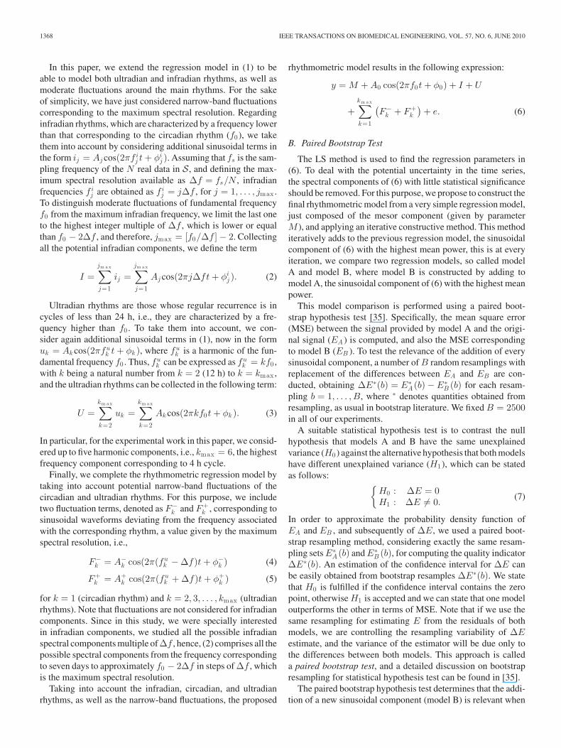
For all the simulations in this section, the original time seriesin S were composed of N = 672 points, obtained by samplingthe original signals with fs = 1/900 Hz (one sample every 15min). To graphically illustrate the effectiveness of the proposedapproach, Fig. 1 shows an example of the original syntheticsignal (periodic square signal) with SNR = 5 dB and the modelestimated by our method, both in time and frequency domains.Specifically, the synthetic signal was obtained as the sum of acontinuous value (M = 0) and six sinusoidal components: Thecircadian component f0 (24 h), two components correspondingto fluctuations of f0 , namely f0 + fs/N and f0 − fs/N Hz,one infradian component corresponding to 2∆f Hz, and twoultradian components 3f0 and 5f0 Hz. Fig. 1(a) shows in thetime domain, the superposition of the original signal (dash line)

Fig. 1. Synthetic example. (a) (Dash) original noisy square signal and (solid)estimated model. (b) (Top) FFT magnitude for the original signal and (bottom)for the estimated signal.

and the estimated model (solid line). Fig. 1(b) corresponds tothe spectral representations in terms of the magnitude of the fastFourier transform (FFT). Note that the model obtained with ourmethod keeps the six spectral components of the original signalwhile discards the noise.

IV. EXPERIMENTS AND RESULTS

We applied the method presented in the previous section tostudy a database of 7-day Holter recordings from patients withCHF, collected in the Arrhythmia Unit of Hospital UniversitarioVirgen de la Arrixaca (Spain). Specifically, the proposed rhyth-mometric procedure was used to analyze some of the most rele-vant HRV markers in the 7-day monitoring database, includingtemporal (AVNN, SDNN, and NN50), spectral (LF, HF, HFn,and LF/HF), and nonlinear (α1 and SampEn) indexes. All theindexes were obtained in time windows of 15 min, yielding alocal description of their time evolution.

The procedure followed for data preprocessing is first pre-sented, and the descriptive statistics of the rhythmometric

1370 IEEE TRANSACTIONS ON BIOMEDICAL ENGINEERING, VOL. 57, NO. 6, JUNE 2010

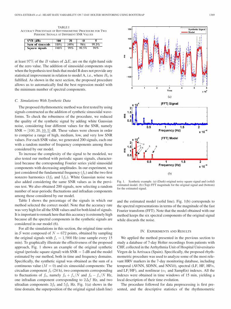
TABLE IIPOPULATION MEAN VALUE ± STANDARD DEVIATION OF RHYTHMOMETRIC MODELS FOR NUMBER OF INFRADIAN AND ULTRADIAN COMPONENTS

(Ni AND Nu ), NUMBER OF FLUCTUATION COMPONENTS (Nf ), PARAMETER %P wt (RELATIVE TO MESOR), AND PARAMETERS

%P wi , %P wu , %P wf , AND %P wf0 (ALL OF THEM RELATIVE TO P wt )

models for each HRV index are reported. Then, the populationaverage spectral profiles of the indexes are presented as wellas the population average time evolution of the indexes duringseven days. In order to characterize the intrinsic daily time fluc-tuations in the patients, the population average time evolutionsof the indexes averaged in 24 h are finally presented. For thesake of clarity in the graphical representations of the populationaverage results, the mean value of the signals and the mesor pa-rameter of the regression models have been removed, and onlypulsatile waveforms are depicted in time plots.

A. Data Preprocessing

Our database consisted of 31 long-term (7-day) Holter record-ings. To analyze the long-term evolution of the HRV markers,the rhythmometric analysis was performed on the NN intervalseries. All data were preprocessed to exclude artifacts and ec-topic beats. Furthermore, the RR intervals lower than 200 msand greater than 2000 ms were excluded, as well as those whichdiffered more than 20% from the previous and the subsequentRR intervals [7].

In order to obtain statistically reliable results, the quality of thedata was examined and low quality recordings were discarded.Specifically, three criteria were established. First, recordingswith less than 80% of sinus beats were discarded (seven record-ings ruled out). Second, the HRV markers were computed at 15min intervals for each patient, by requiring each 15-min segmentto have itself more than 80% of valid sinus beats to compute themarkers. Finally, the third criterion limited to 80% the minimumpercentage of usable 15-min segments to consider the recordingsuitable for the analysis (two recordings ruled out). The use ofthese criteria resulted in a final population of 22 patients.

B. Computing HRV Indexes

We computed the HRV indexes in 15-min windows by delet-ing the nonsinus beats in the case of temporal and nonlinearindexes, and from evenly resampled NN intervals using linearinterpolation in the case of the spectral indexes. Hence, spectralindexes were preserved with respect to their time reference.

C. Descriptive Statistics for Rhythmometric Models

Table II shows the population statistics (mean and standarddeviation) of the number of sinusoidal components provided

by the rhythmometric method. In particular, the number of in-fradian components (Ni), the number of ultradian components(Nu ), and the number of fluctuations (Nf ) are presented for allthe indexes. To determine the performance of the rhythmomet-ric method, parameter Pwt was obtained for representing thepercentage of increase in the total explained variance when theregression model just considering the mesor component (initialmodel) was replaced by the final rhythmometric model. To eval-uate the contribution of every kind of spectral component to thefinal regression model, we considered the corresponding valueof Pwt as the base reference for all the indexes, and we de-termined the percentage of Pwt corresponding to the infradiancomponents (%Pwi), to the ultradian components (%Pwu ),to the fluctuations (%Pwf ), and to the circadian component(%Pwf 0).

The results show that populationally and for all the indexes,the component with the highest contribution to the increase inthe explained variance was circadian component f0 , followedin importance by infradian, ultradian, and fluctuation compo-nents. For infradian components, they contributed in 66% ofthe indexes to an increase of more than 25% of the explainedpower. Fluctuations also represent a significant, though less no-ticeable percentage of Pwt for most indexes. AVNN, NN50,SampEn, and HF indexes were modeled with higher numberof spectral components, and also presented higher Pwt , whichindicates that these indexes are better described by a rhythmo-metric model than the others. It is remarkable that in this lastgroup of indexes, we have at least one index of each HRV familyof indexes (temporal, spectral, and nonlinear).

D. Population Average Spectra of HRV Indexes in Seven Days

Fig. 2 details the spectral profiles of the original HRV indexesand those provided by our rhythmometric models. Note that therhythmometric models retain the main spectral components ofthe original signals while canceling most of the noise. Popula-tionally, the circadian component was the main one for all the in-dexes, as seen in Table II. Infradian components were markedlypresent in all the indexes, but predominantly in NN50, HF,HFn, LF/HF, α1 , and SampEn, showing evidence of rhythmsthat affect the state of the ANS additionally to circadian andultradian rhythms. The most significant infradian component isemphasized through an arrow in Fig. 2, however, note that alsoother infradian components can be significant. All the indexes

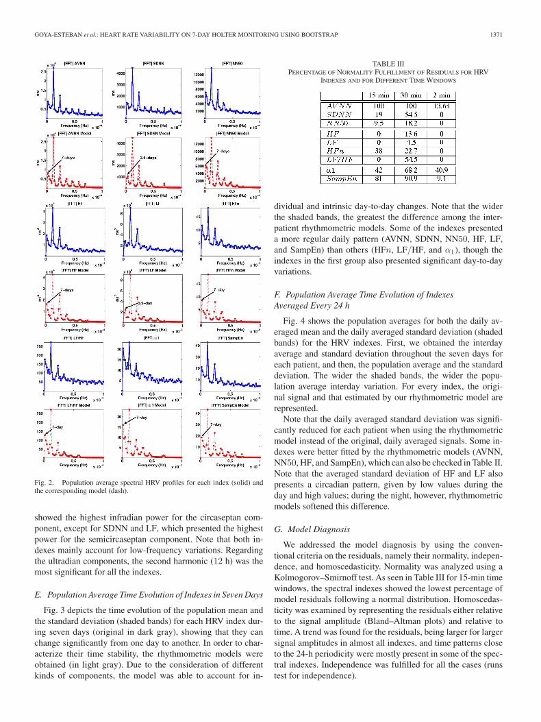
GOYA-ESTEBAN et al.: HEART RATE VARIABILITY ON 7-DAY HOLTER MONITORING USING BOOTSTRAP 1371

Fig. 2. Population average spectral HRV profiles for each index (solid) andthe corresponding model (dash).

showed the highest infradian power for the circaseptan com-ponent, except for SDNN and LF, which presented the highestpower for the semicircaseptan component. Note that both in-dexes mainly account for low-frequency variations. Regardingthe ultradian components, the second harmonic (12 h) was themost significant for all the indexes.

E. Population Average Time Evolution of Indexes in Seven Days

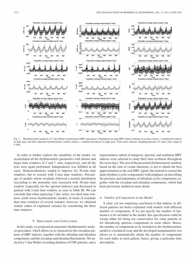
Fig. 3 depicts the time evolution of the population mean andthe standard deviation (shaded bands) for each HRV index dur-ing seven days (original in dark gray), showing that they canchange significantly from one day to another. In order to char-acterize their time stability, the rhythmometric models wereobtained (in light gray). Due to the consideration of differentkinds of components, the model was able to account for in-

TABLE IIIPERCENTAGE OF NORMALITY FULFILLMENT OF RESIDUALS FOR HRV

INDEXES AND FOR DIFFERENT TIME WINDOWS

dividual and intrinsic day-to-day changes. Note that the widerthe shaded bands, the greatest the difference among the inter-patient rhythmometric models. Some of the indexes presenteda more regular daily pattern (AVNN, SDNN, NN50, HF, LF,and SampEn) than others (HFn, LF/HF, and α1), though theindexes in the first group also presented significant day-to-dayvariations.

F. Population Average Time Evolution of IndexesAveraged Every 24 h

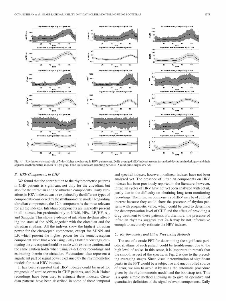
Fig. 4 shows the population averages for both the daily av-eraged mean and the daily averaged standard deviation (shadedbands) for the HRV indexes. First, we obtained the interdayaverage and standard deviation throughout the seven days foreach patient, and then, the population average and the standarddeviation. The wider the shaded bands, the wider the popu-lation average interday variation. For every index, the origi-nal signal and that estimated by our rhythmometric model arerepresented.

Note that the daily averaged standard deviation was signifi-cantly reduced for each patient when using the rhythmometricmodel instead of the original, daily averaged signals. Some in-dexes were better fitted by the rhythmometric models (AVNN,NN50, HF, and SampEn), which can also be checked in Table II.Note that the averaged standard deviation of HF and LF alsopresents a circadian pattern, given by low values during theday and high values; during the night, however, rhythmometricmodels softened this difference.

G. Model Diagnosis

We addressed the model diagnosis by using the conven-tional criteria on the residuals, namely their normality, indepen-dence, and homoscedasticity. Normality was analyzed using aKolmogorov–Smirnoff test. As seen in Table III for 15-min timewindows, the spectral indexes showed the lowest percentage ofmodel residuals following a normal distribution. Homoscedas-ticity was examined by representing the residuals either relativeto the signal amplitude (Bland–Altman plots) and relative totime. A trend was found for the residuals, being larger for largersignal amplitudes in almost all indexes, and time patterns closeto the 24-h periodicity were mostly present in some of the spec-tral indexes. Independence was fulfilled for all the cases (runstest for independence).

1372 IEEE TRANSACTIONS ON BIOMEDICAL ENGINEERING, VOL. 57, NO. 6, JUNE 2010

Fig. 3. Rhythmometric analysis of 7-day Holter monitoring in HRV parameters. Population average HRV indexes during seven days (mean ± standard deviation)in dark gray and their adjusted rhythmometric models (mean ± standard deviation) in light gray. Time units indicate sampling periods (15 min), time origin at9 AM.

In order to further explore the suitability of the model, werecalculated all the rhythmometric parameters with shorter andlarger time windows of 2 and 3 -min, respectively, and all thetests were again performed. Independence was fulfilled in allcases. Homoscedasticity tended to improve for 30-min timewindows, but to worsen with 2-min time windows. Percent-age of models whose residuals followed a normal distribution(according to the normality test) increased with 30-min timewindow (especially for the spectral indexes) and decreased ingeneral with 2-min time window, as seen in Table III. We canconclude that when analyzing 7-day series, too short time win-dows yield worse rhythmometric models, in terms of residualsthan time windows of several minutes, however, we obtainedsimilar values of explained variance by considering the threetime windows.

V. DISCUSSION AND CONCLUSION

In this study, we proposed an automatic rhythmometric analy-sis procedure, which allows us to characterize the circadian pat-terns of HRV indexes, together with the infradian and ultradiancomponents, and the circadian and ultradian fluctuations. We an-alyzed a 7-day Holter recording database of CHF patients, and a

representative subset of temporal, spectral, and nonlinear HRVindexes were selected to study their time evolution throughoutthe seven days. The aim of the presented rhythmometric method,based on the sum of cosine functions, is not to obtain the bestapproximation to the real HRV signal, but instead to extract themain rhythms (cyclic components) with emphasis on describingthe presence and importance of infradian cyclic components, to-gether with the circadian and ultradian components, which hadbeen previously studied in more detail.

A. Number of Components in the Model

A clear, yet not surprising conclusion is that indexes in dif-ferent patients are better explained with models with differentnumber of components. If we per-specify the number of har-monics to be included in the model, this specification could bewrong either for being too conservative for some patients orfor introducing spurious components in some others. Hence,the number of components to be included in the rhythmometricmodel is a technical issue and the developed nonparametric testallows us to automatically obtain the number of componentsfor each index in each patient, hence, giving a particular timedescription.

GOYA-ESTEBAN et al.: HEART RATE VARIABILITY ON 7-DAY HOLTER MONITORING USING BOOTSTRAP 1373

Fig. 4. Rhythmometric analysis of 7-day Holter monitoring in HRV parameters. Daily averaged HRV indexes (mean ± standard deviation) in dark gray and theiradjusted rhythmometric models in light gray. Time units indicate sampling periods (15 min), time origin at 9 AM.

B. HRV Components in CHF

We found that the contribution to the rhythmometric patternsin CHF patients is significant not only for the circadian, butalso for the infradian and the ultradian components. Daily vari-ations in HRV indexes can be explained by the different types ofcomponents considered by the rhythmometric model. Regardingultradian components, the 12 h component is the most relevantfor all the indexes. Infradian components are markedly presentin all indexes, but predominantly in NN50, HFn, LF/HF, α1 ,and SampEn. This shows evidence of infradian rhythms affect-ing the state of the ANS, together with the circadian and theultradian rhythms. All the indexes show the highest ultradianpower for the circaseptan component, except for SDNN andLF, which present the highest power for the semicircaseptancomponent. Note that when using 7-day Holter recordings, esti-mating the circaseptanshould be made with extreme caution, andthe same caution holds when using 24-h Holter recordings andestimating therein the circadian. Fluctuations also represent asignificant part of signal power explained by the rhythmometricmodels for most HRV indexes.

It has been suggested that HRV indexes could be used forprognosis of cardiac events in CHF patients, and 24-h Holterrecordings have been used to estimate these indexes. Circa-dian patterns have been described in some of these temporal

and spectral indexes, however, nonlinear indexes have not beenanalyzed yet. The presence of ultradian components on HRVindexes has been previously reported in the literature, however,infradian cycles of HRV have not yet been analyzed with detail,partly due to the difficulty on obtaining long-term monitoringrecordings. The infradian components of HRV may be of clinicalinterest because they could show the presence of rhythm pat-terns with prognostic value, which could be used to determinethe decompensation level of CHF and the effect of providing adrug treatment to these patients. Furthermore, the presence ofinfradian rhythms suggests that 24 h may be not informativeenough to accurately estimate the HRV indexes.

C. Rhythmometry and Other Processing Methods

The use of a crude FFT for determining the significant peri-odic rhythms of each patient could be troublesome, due to thehigh level of noise. In this sense, it is important to remark thatthe smooth aspect of the spectra in Fig. 2 is due to the preced-ing averaging stages. Since visual determination of significantpeaks in the FFT would be a subjective and uncontrolled sourceof error, we aim to avoid it by using the automatic proceduregiven by the rhythmometric model and the bootstrap test. Thisis a quite simple method allowing us to give an operative andquantitative definition of the signal relevant components. Daily

1374 IEEE TRANSACTIONS ON BIOMEDICAL ENGINEERING, VOL. 57, NO. 6, JUNE 2010

summaries might also be used for giving a useful descriptionof the temporal changes in a given index, however, unless verycarefully chosen, these summaries could be discarding somerelevant information, specially, the presence of infradian com-ponents or near-periodic fluctuations of ultradian components.To our understanding, the proposed method is a principled ap-proach for characterizing the rhythmometric components.

Though the proposed rhythmometric model may not be thebest regression model in terms of the lowest prediction error, italways provides clear information about the presence of ultra-dian and infradian rhythms. Day-by-day changes are present inthe model in two forms, namely the narrow-band fluctuations inthe circadian and ultradian components, and the infradian com-ponents. Previous rhythmometric models mostly used a singlecosine model (cosinor) or at most, a set of cosine functionsfor the harmonics, to study the circadian variation of differentphysiological data, aiming to study the presence of daily cyclicvariations [11], [17]. These previous rhythmometric models didnot consider these described fluctuations. Note that the use of arhythmometric model while simple, does not exclude the possi-ble use of other methods, such as autoregressive models [8].

Finally, there exist other processing methods, such as per-forming long-term continuous monitoring of HRV indexes fromimplanted devices. This method has proved to be a useful toolproviding prognostic information about patient mortality, infor-mation that may be helpful for risk stratification [36].

D. Effect of Signal Length

Comparisons among different studies with the proposedmodel should take into account the signal duration and the timewindow duration for computing HRV indexes. However, notethat if we call sampling frequency fs to the inverse of the av-eraging time window for obtaining the HRV indexes from theNN interval series, and denoting as D the total duration (in sec-onds) of NN interval series, hence, the length in samples N ofeach HRV index signal depends on fs . Note that assuming thatNyquist holds for the same D, the use of different time windowswill give the same spectral resolution ∆f = 1/D. Hence, thefluctuation components can be considered to be independentof the sampling frequency whenever the length of every NNrecording is the same. Though more adjacent frequencies couldbe included in the model for the narrow-band fluctuations (forinstance, up to 2∆f or 3∆f ), we used only up to ∆f becausepopulation spectral peaks were mostly about this width.

E. Limitations of the Study

The proposed rhythmometric model gives a set of parameterscharacterizing the long-term rhythmometric evolution for sevendays time series. For these parameters being useful in risk strat-ification, a specific study and followup should be addressed,which is beyond the scope of this descriptive study. Though inthis paper, we only report the results for the analysis with 15-minsegments, we increased the number of harmonics considered byour approach and performed an additional study based on 2-min segments. A comparison between both studies revealedthat inspite of the analysis with shorter segments provided more

significant ultradian components, these new ultradian compo-nents had relatively small amplitude and the population totalexplained variance remained nearly the same in both studies.The temporary presence of sleep cycles, previously reportedin [12], was not detected by our method, likely due to those ul-tradian cycles are only present in some sleeping periods. Thus,for the proposed method being capable of detecting those cy-cles, the temporal series should be constrained to some nightperiods that we have not considered because in this paper, wewanted to focus on a stationary description throughout severalconsecutive complete days.

In relation to the day of week when the recordings were starteddue to clinical reasons, not all recordings were started the sameday of week. This fact could cause a smoothing on the infradiantrends in the representation of Fig. 3 (because population aver-ages are computed). Nevertheless, since a rhythmometric modelwas obtained separately for each recording, it was possible todetect the infradian components in the signals as can be seen inthe extracted statistics (see Table II) and in the spectral profilesof the models (see Fig. 2).

Finally, a database of CHF patients has been used for therhythmometric analysis in this paper. However, we considerthat further studies with long-term databases, including controlgroups will be highly informative.

F. Conclusion

The long-term analysis of cardiac series is probably becomingin the near future an active research area, either from long-termHolter or from implantable devices, or from other sources. Themain contribution of this paper has been the proposal of an auto-matic procedure for giving a rhythmometric model able to dealwith this kind of long-term series, which gives the cyclostation-ary nature of cardiac indexes, is expected to be useful for thiskind of analysis.

REFERENCES

[1] E. Seto, “Cost comparison between telemonitoring and usual care of heartfailure: A systematic review,” Telemed. J. E. Health, vol. 14, no. 7,pp. 679–686, 2008.

[2] A. Martınez, E. Everss, J. L. Rojo-Alvarez, D. P. Figal, and A. Garcıa-Alberola, “A systematic review of the literature on home monitoring forpatients with heart failure,” J. Telemed Telecare, vol. 12, no. 5, pp. 234–241, 2006.

[3] N. Maglaveras, I. Lekka, I. Chouvarda, D. Adamidis, H. Karvounis,G. Louridas, B. Zeevi, and E. A. Balas, “Congestive heart failure man-agement in a home-care system through the chs contact center,” Comput.Cardiol., vol. 30, pp. 189–192, 2003.

[4] D. Steven, T. Rostock, B. Lutomsky, H. Klemm, H. Servatius, I. Drewitz,K. Friedrichs, R. Ventura, T. Meinertz, and S. Willems, “What is the realatrial fibrillation burden after catheter ablation of atrial fibrillation? Aprospective rhythm analysis in pacemaker patients with continuous atrialmonitoring,” Eur. Heart J., vol. 29, no. 8, pp. 1037–1042, 2008.

[5] N. Dagres, H. Kottkamp, C. Piorkowski, S. Weis, A. Arya, P. Sommer,K. Bode, J.-H. Gerds Li, D. T. Kremastinos, and G. Hindricks, “Influenceof the duration of holter monitoring on the detection of arrhythmia recur-rences after catheter ablation of atrial fibrillation: Implications for patientfollow-up,” Int. J. Cardiol., DOI: 10.1016/j.ijcard.2008.10.004.

[6] D. Jabaudon, J. Sztajzel, K. Sievert, T. Landis, and R. Sztajzel, “Usefulnessof ambulatory 7-day ECG monitoring for the detection of atrial fibrillationand flutter after acute stroke and transient ischemic attack,” Stroke, vol. 35,no. 7, pp. 1647–1651, 2004.

GOYA-ESTEBAN et al.: HEART RATE VARIABILITY ON 7-DAY HOLTER MONITORING USING BOOTSTRAP 1375

[7] M. Malik, T. Cripps, T. Farrell, and A. Camm, “Prognostic value of heartrate variability after myocardial infarction. A comparison of differentdata-processing methods,” MBEC, vol. 27, no. 6, pp. 603–611, 1989.

[8] M. Malik, J. Bigger, A. Camm, R. Kleiger, A. Malliani, A. Moss, andP. Schwartz, “Heart rate variability standards of measurement, physio-logical interpretation, and clinical use,” Eur. Heart J., vol. 17, no. 3,pp. 354–381, 1996.

[9] H. V. Huikuri, J. O. Valkama, K. E. Airaksinen, T. Seppanen, K.M. Kessler, J. T. Takkunen, and R. J. Myerburg, “Frequency domainmeasures of heart rate variability before the onset of nonsustained andsustained ventricular tachycardia in patients with coronary artery disease,”Circulation, vol. 87, no. 4, pp. 1220–1228, 1993.

[10] H. V. Huikuri, M. J. Niemela, S. Ojala, A. Rantala, M. J. Ikaheimo, andK. E. Airaksinen, “Circadian rhythms of frequency domain measures ofheart rate variability in healthy subjects and patients with coronary arterydisease, effects of arousal and upright posture,” Circulation, vol. 90, no. 1,pp. 121–126, 1994.

[11] M. M. Massin, K. Maeyns, N. Withofs, F. Ravet, and P. Gerard, “Circadianrhythm of heart rate and heart rate variability,” Br. Med. J., vol. 83, no. 2,pp. 179–182, 2000.

[12] P. K. Stein, E. J. Lundequam, D. Clauw, K. E. Freedland, R. M. Carney, andP. P. Domitrovich, “Circadian and ultradian rhythms in cardiac autonomicmodulation,” IEEE Eng. Med. Biol. Mag., vol. 26, no. 6, pp. 14–18,Nov./Dec. 2007.

[13] A. Delyukov, Y. Gorgo, G. Cornelissen, K. Otsuka, and F. Halberg, “Nat-ural environmental associations in a 50-day human electrocardiogram,”Int. J. Biometeorol., vol. 45, no. 2, pp. 90–99, 2001.

[14] A. Delyukov, Y. Gorgo, G. Cornelissen, K. Otsuka, and F. Halberg, “Infra-dian, notably circaseptan testable feedsidewards among chronomes of theECG and air temperature and pressure,” Biomed. Pharmacother., vol. 55,pp. 84s–92s, 2001.

[15] Y. F. Guo and P. K. Stein, “Circadian rhythm in the cardiovascular sys-tem: Chronocardiology,” Amer. Heart J., vol. 145, no. 5, pp. 779–786,2003.

[16] R. Singh, G. Cornelissen, A. Weydahl, O. Schwartzkopff, G. Katinas,K. Otsuka, Y. Watanabe, S. Yano, H. Mori, Y. Ichimaru et al., “Circadianheart rate and blood pressure variability considered for research and patientcare,” Int. J. Cardiol., vol. 87, no. 1, pp. 9–28, 2003.

[17] R. C. Hermida, D. E. Ayala, and F. Portaluppi, “Circadian variation ofblood pressure: The basis for the chronotherapy of hypertension,” Adv.Drug Del. Rev., vol. 59, no. 9–10, pp. 904–922, 2007.

[18] F. Portaluppi and R. C. Hermida, “Circadian rhythms in cardiac arrhyth-mias and opportunities for their chronotherapy,” Adv. Drug Del. Rev.,vol. 59, no. 9–10, pp. 940–951, 2007.

[19] M. Smolensky and N. Peppas, “Chronobiology, drug delivery, andchronotherapeutics,” Adv. Drug Del. Rev., vol. 59, no. 9–10, pp. 828–851, 2007.

[20] A. Bilan, A. Witczak, R. Palusinski, W. Myslinski, and J. Hanzlik, “Circa-dian rhythm of spectral indices of heart rate variability in healthy subjects,”J. Electrocardiol., vol. 38, no. 3, pp. 239–243, 2005.

[21] G. Q. Wu, L. L. Shen, D. K. Tang, D. A. Zheng, and C. S. Poon, “Circadianrhythms of spectral components of heart rate variability,” in Proc. Conf.Proc. IEEE Eng. Med. Biol. Soc., 2006, vol. 1, pp. 3557–3560.

[22] J. E. Mietus, C.-K. Peng, I. Henry, R. L. Goldsmith, and A. L. Goldberger,“The pNNx files: Re-examining a widely used heart rate variability mea-sure,” Heart, vol. 88, no. 4, pp. 378–380, 2002.

[23] S. Akselrod, D. Gordon, F. A. Ubel, D. C. Shannon, A. C. Berger, andR. J. Cohen, “Power spectrum analysis of heart rate fluctuation: A quan-titative probe of beat-to-beat cardiovascular control,” Science, vol. 213,no. 4504, pp. 220–222, 1981.

[24] S. Cerutti, A. M. Bianchi, and L. T. Mainardi, “Spectral analysis of theheart rate variability,” in Heart Rate Variability, M. Malik and A. J. Camm,Eds. New York: Futura Publishing Company, 1995.

[25] C. F. Notarius and J. S. Floras, “Limitations of the use of spectral analysisof heart rate variability for the estimation of cardiac sympathetic activityin heart failure,” Europace, vol. 3, no. 1, pp. 29–38, 2001.

[26] J. A. Taylor, D. L. Carr, C. W. Myers, and D. L. Eckberg, “Mechanismsunderlying very-low-frequency RR-interval oscillations in humans,” Cir-culation, vol. 98, no. 6, pp. 547–555, 1998.

[27] A. L. Goldberger, “Is the normal heartbeat chaotic or homeostatic?,” NewsPhysiol. Sci., vol. 6, pp. 87–91, 1991.

[28] H. V. Huikuri, T. Makikallio, C. Peng, A. L. Goldberger, U. Hintze, andM. Moller, “Fractal correlation properties of RR interval dynamics andmortality in patients with depressed left ventricular function after an acutemyocardial infarction,” Circulation, vol. 101, pp. 47–53, 2000.

[29] S. M. Pincus, “Approximate entropy as a measure of system complexity,”Proc. Nat. Acad. Sci., vol. 88, pp. 2297–2301, 1991.

[30] R. Singh, G. Cornelissen, J. Siegelova, P. Homolka, and F. Halberg, “Abouthalf-weekly (circasemiseptan) pattern in blood pressure and heart rate inmen and women of india,” Scripta Medica, vol. 75, no. 3, pp. 125–128,2002.

[31] G. Cornelissen, T. Breus, C. Bingham, R. Zaslavskaya, M. Varshitsky,B. Mirsky, M. Teilbloom, B. Tarquini, E. Bakken, and F. Halberg, “Be-yond circadian chronorisk: Worldwise circaseptan-circasemiseptan pat-terns of myocardial infarctions, other vascular events, and emergencies,”Chronobiologia, vol. 20, pp. 87–115, 1993.

[32] C. Peng, S. Havlin, H. Stanley, and A. Goldberger, “Quantification ofscaling exponents and crossover phenomena in nonstationary heartbeattime series,” Chaos, vol. 5, no. 1, pp. 82–87, 1995.

[33] J. Richman and J. Moorman, “Physiological time-series analysis usingapproximate entropy and sample entropy,” Amer. J. Physiol.-Heart Circ.Physiol., vol. 278, no. 6, pp. 2039–2049, 2000.

[34] A. Mojon, J. R. Fernandez, and R. C. Hermida, “Chronolab: An interactivesoftware package for chronobiologic time series analysis written for themacintosh computer,” Chronobiol. Int., vol. 9, no. 6, pp. 403–412, 1992.

[35] B. Efron and R. Tibshirani, An Introduction to the Bootstrap. London,U.K.: Chapman & Hall, 1993.

[36] F. R. Gilliam, J. P. Singh, C. M. Mullin, M. McGuire, and K. J. Chase,“Prognostic value of heart rate variability footprint and standard devia-tion of average 5-minute intrinsic RR intervals for mortality in cardiacresynchronization therapy patients,” J. Electrocardiol., vol. 40, no. 4,pp. 336–342, 2007.

Rebeca Goya-Esteban received the Tech. Telecom.Eng. degree in technical telecommunication engi-neering from Universidad Carlos III de Madrid,Madrid, Spain, in 2006, and the M.Sc. degree inbiomedical engineering from Universidade do Porto,Porto, Portugal, in 2008.

She is currently in the Department of SignalTheory and Communications, Universidad Rey JuanCarlos, Madrid. Her research interests include lin-ear and nonlinear time-series analysis and long termmonitoring analysis of cardiac electric signals.

Inmaculada Mora-Jimenez received the Telecom.Eng. degree in telecommunication engineering fromUniversidad Politecnica de Valencia, Valencia, Spain,in 1998, and the Ph.D. degree from UniversidadCarlos III de Madrid, Madrid, Spain, in 2004.

She is currently an Associate Professor in theDepartment of Signal Theory and Communications,Universidad Rey Juan Carlos, Madrid. Her researchinterests include statistical learning theory, neuralnetworks and their applications to image processing,bioengineering and communications.

Jose Luis Rojo-Alvarez (M’01) received the Telecom. Eng. degree in telecom-munication engineering from Universidad de Vigo, Galicia, Spain, in 1996, andthe Ph.D. degree in telecommunication from Universidad Politecnica de Madrid,Madrid, Spain, in 2000.

Since 2006, he has been an Associate Professor in the Department of SignalTheory and Communications, Universidad Rey Juan Carlos, Madrid. He hasauthored or coauthored more than 120 papers and communications. His cur-rent research interests include statistical learning theory and complex systemmodeling with applications to communications and cardiac signal, and imageprocessing.

1376 IEEE TRANSACTIONS ON BIOMEDICAL ENGINEERING, VOL. 57, NO. 6, JUNE 2010

Oscar Barquero-Perez received the Tech. Telecom. Eng. degree in technicaltelecommunication engineering from Universidad Carlos III de Madrid, Madrid,Spain, in 2005, and the M.Sc. degree in biomedical engineering from Universi-dade do Porto, Porto, Portugal, in 2008.

Since 2007, he has been with the Department of Signal Theory and Com-munications, Universidad Rey Juan Carlos, Madrid. His current research in-terests include linear and nonlinear time-series analysis, and biomedical signalprocessing.

Francisco J. Pastor-Perez received the M.D. degree from Universidad deMurcia, Murcia, Spain, in 2002.

He specialized in cardiology in 2009 and is currently engaged with HospitalUniversitario Virgen de la Arrixaca, Murcia. His research interests include heartfailure and new mechanism of risk stratification using cardiac signals analysis.

Sergio Manzano-Fernandez received the M.D. degree from Universidad deMurcia, Murcia, Spain, in 2005.

Since 2005, he has been a Cardiologist at Hospital Universitario Virgende la Arrixaca, Murcia. His current research interests include anticoagulationtherapy and major bleeding complications in patients with atrial fibrillation, andprognostic value of biomarkers in heart failure.

Domingo A. Pascual-Figal received the M.D. degreefrom Universidad de Salamanca, Salamanca, Spain,in 1993, and the Ph.D. degree from Universidad deMurcia, Murcia, Spain, in 1999.

He is currently with the Hospital UniversitarioVirgen de la Arrixaca, Murcia, and also an AssociateProfessor at the Universidad de Murcia, Murcia. Hehas authored or coauthored more than 70 original sci-entific articles. His research interests include clinicalcardiology, focused on heart failure, biomarkers, andcardiac monitorization.

Arcadi Garcıa-Alberola received the M.D. and Ph.D. degrees from Universidadde Valencia, Valencia, Spain, in 1982 and 1991, respectively.

Since 1993, he has been a Cardiologist and a Professor of Medicine atHospital Universitario Virgen de la Arrixaca and Universidad de Murcia, Spain,respectively. He has authored or coauthored more than 120 scientific papers incardiac electrophysiology. His current research interests include repolarizationanalysis, arrhythmia mechanisms, and cardiac signal processing.