Active Manipulation for Perception

Anna Petrovskaya∗and Kaijen Hsiao†∗Stanford University, USA, †Bosch Research and Technology Center, Palo Alto, USA

September 1, 2016

Abstract

This chapter covers perceptual methods in which ma-nipulation is an integral part of perception. Thesemethods face special challenges due to data spar-sity and high costs of sensing actions. However, theycan also succeed where other perceptual methods fail,e.g., in poor-visibility conditions or for learning thephysical properties of a scene.

The chapter focuses on specialized methods thathave been developed for object localization, inference,planning, recognition, and modeling in active manip-ulation approaches. We conclude with a discussionof real-life applications and directions for future re-search.

1

Contents

42 Active Manipulation for Perception 442.1 Object Localization . . . . . . . . . . . 5

42.1.1 Problem Evolution . . . . . . . 542.1.2 Bayesian Framework . . . . . . 642.1.3 Inference . . . . . . . . . . . . 942.1.4 Advanced Inference Methods . 1142.1.5 Planning . . . . . . . . . . . . 13

42.2 Learning About An Object . . . . . . 1942.2.1 Shape of Rigid Objects . . . . 1942.2.2 Articulated Objects . . . . . . 2142.2.3 Deformable Objects . . . . . . 2342.2.4 Contact Estimation . . . . . . 2342.2.5 Physical Properties . . . . . . . 25

42.3 Recognition . . . . . . . . . . . . . . . 2542.3.1 Object shape matching . . . . 2642.3.2 Statistical pattern recognition . 2642.3.3 Recognition by material prop-

erties . . . . . . . . . . . . . . 2742.3.4 Combining visual and tactile

sensing . . . . . . . . . . . . . 2742.4 Conclusions . . . . . . . . . . . . . . . 28

42.4.1 Real-Life Applications . . . . . 2842.4.2 Future Directions of Research . 2942.4.3 Further Reading . . . . . . . . 29

References . . . . . . . . . . . . . . . . . . . 30Index . . . . . . . . . . . . . . . . . . . . . 36

2

List of Figures

42.1 Objects and their models . . . . . . . 742.2 Bayesian Networks . . . . . . . . . . . 742.3 Sampled measurement models . . . . . 842.4 Peak width and annealing . . . . . . . 1242.5 Planning Bayesian Netowrk . . . . . . 1442.6 Action selection . . . . . . . . . . . . . 1642.7 Multi-step planning . . . . . . . . . . 1742.8 Robot grasping a powerdrill . . . . . . 1842.9 Underwater mapping . . . . . . . . . . 2042.10Object represented by splines . . . . . 2142.11Occupancy grid representation . . . . 2242.12 Articulated object examples . . . . . 2242.13 Exploring articulated objects . . . . . 2242.14 A 2D deformable object . . . . . . . . 2342.15 A 3D deformable object . . . . . . . . 2342.16 Contact estimation . . . . . . . . . . 2442.17 Tactile images of objects . . . . . . . 2742.18 Vocabulary of tactile images . . . . . 27

3

Chapter 42

Active Manipulation for Perception

In this chapter, we focus on perceptual methodsthat rely on manipulation. As we shall see, sensing-via-manipulation is a complex and highly intertwinedprocess, in which the results of perception are used formanipulation and manipulation is used to gather ad-ditional data. Despite this complexity, there are threemain reasons to use manipulation either together orinstead of the more commonly used vision sensors.

First, manipulation can be used to sense in poor-visibility conditions: for example, sensing in muddywater or working with transparent objects. In fact,due to its high accuracy and ability to sense anyhard surface regardless of its optical properties, con-tact sensing is widely used for accurate localizationof parts in manufacturing. Second, manipulation isuseful for determining properties that require physi-cal interaction, such as stiffness, mass, or the physicalrelationship of parts. Third, if the actual goal is tomanipulate the object, we may as well use data gath-ered from manipulation attempts to improve bothperception and subsequent attempts at manipulation.

Sensing-via-manipulation also faces significantchallenges. Unlike vision sensors, which provide awhole-scene view in a single snapshot, contact sen-sors are inherently local, providing information onlyabout a very small area of the sensed surface at anygiven time. In order to gather additional data, themanipulator has to be moved into a different posi-tion, which is a time-consuming task. Hence, unlikevision-based perception, contact-based methods haveto cope with very sparse data and very low data ac-quisition rates. Moreover, contact sensing disturbs

the scene. While in some situations this can be de-sirable, it also means that each sensing action can in-crease uncertainty. In fact, one can easily end up ina situation where the information gained via sensingis less than the information lost due to scene distur-bance.

Due to these challenges, specialized perceptualmethods had to be developed for perception-via-manipulation. Inference methods have been devel-oped to extract the most information from the scarcedata and to cope with cases in which the data areinsufficient to fully solve the problem (i.e., under-constrained scenarios). Planning methods have beendeveloped to make the most efficient sensing decisionsbased on the little data available and taking into ac-count time, energy, and uncertainty costs of sensingactions. Modeling methods have been developed tobuild the most accurate models from small amountsof data.

In our discussion, the material is organized by per-ceptual goal: localizing an object — Sect. 42.1, learn-ing about an object — Sect. 42.2, and recognizing anobject — Sect. 42.3. Since the chapter topic is broad,to keep it concise, we provide a tutorial-level discus-sion of object localization methods, but give a birds-eye view of the methods for the other two perceptualgoals. However, as we point out along the way, manyobject localization methods can be re-used for theother two perceptual goals.

4

42.1 Object Localization

Tactile object localization is the problem of estimat-ing the object’s pose — including position and orien-tation — based on a set of data obtained by touchingthe object. A prior geometric model of the object isassumed to be known and the sensing is performedusing some type of contact sensor (wrist force/torquesensor, tactile array, fingertip force sensor, etc). Theproblem is typically restricted to rigid objects, whichcan be stationary or moving.

Tactile object localization involves several compo-nents, including manipulator control methods, mod-eling, inference, and planning. During data collec-tion, some form of sensorimotor control is used foreach sensing motion of the manipulator. For informa-tion on manipulator control, the reader is encouragedto reference Chapters 8(1) and 9(2). With few excep-tions, the sensing motions tend to be poking motionsrather than following the surface. This is due to thefact that robots are usually unable to sense with allparts of the manipulator, and, hence, the poking mo-tions are chosen to minimize the possibility of acci-dental non-sensed contact.

Due to the properties of sensing-via-contact, spe-cial methods for modeling, inference, and planninghad to be developed for tactile localization. Model-ing choices include not only how to model the objectitself, but also models of the sensing process and mod-els of possible object motion. We discuss models ofsensing and motion in Sect. 42.1.2, but leave an in-depth discussion of object modeling techniques untilSect. 42.2. We also cover specialized inference andplanning methods in Sects. 42.1.3 and 42.1.5 respec-tively.

42.1.1 Problem Evolution

Attempts to solve the tactile object localization dateback to early 80s. Over the years, the scope of theproblem as well as methods used to solve it haveevolved as we detail below.

(1)Chap 8 “Motion Control”(2)Chap 9 “Force Control”

Early Methods

Early methods for tactile object localization generallyignore the sensing process uncertainties and focus onfinding a single hypothesis that best fits the mea-surements. For example, Gaston and Lozano-Perezused interpretation trees to efficiently find the bestmatch for 3DOF object localization [1]. Grimson andLozano-Perez extended the approach to 6DOF [2].Faugeras and Hebert used least squares to performgeometrical matching between primitive surfaces [3].Shekhar et al. solved systems of weighted linear equa-tions to localize an object held in a robotic hand [4].Several methods use geometric constraints togetherwith kinematic and dynamic equations to estimate orconstrain the pose of known planar objects in planeby pushing them with a finger [5] or parallel-jaw grip-per [6], or by tilting them in a tray [7].

Workpiece Localization

Single hypothesis methods are also widely used tosolve the workpiece localization problem in manu-facturing applications for dimensional inspection [8],machining [9], and robotic assembly [10]. In theseapplications, the measurements are taken by a coor-dinate measurement machine (CMM ) [11] or by on-machine sensors [12]. Workpiece localization makesa number of restrictive assumptions that make itinapplicable to autonomous robot operation in un-structured environments. One important restrictionis that there is a known correspondence between eachmeasured data point and a point or patch on the ob-ject surface (called home point or home surface re-spectively) [13]. In semi-automated settings, the cor-respondence assumption is satisfied by having a hu-man direct the robot to specific locations on the ob-ject. In fully-automated settings, the object is placedon the measurement table with low uncertainty tomake sure each data point lands near the correspond-ing home point.

Further restrictions include assumptions that thedata are sufficient to fully constrain the object, theobject does not move, and there are no unmodeledeffects (e.g., vibration, deformation, or temperaturevariation). All of these parameters are carefully con-

5

trolled for in structured manufacturing environments.

The workpiece localization problem is usuallysolved in least squares form using iterative optimiza-tion methods, including the Hong-Tan method [14],the Variational method [15], and the Menq method[16]. Since these methods are prone to gettingtrapped in local minima, low initial uncertainty isusually assumed to make sure the optimization algo-rithm is initialized near the solution. Some attemptshave been made to solve the global localization prob-lem by re-running the optimization algorithm multi-ple times from pre-specified and random initial points[17]. Recent work has focused on careful selectionof the home points to improve localization results[18, 19, 20] and on improving localization efficiencyfor complex home surfaces [21, 22].

Bayesian Methods

In the last decade, there has been increased interestin Bayesian state estimation for the tactile object lo-calization problem [23, 24, 25, 26, 27]. These methodsestimate the probability distribution over all possiblestates (the belief), which captures the uncertaintyresulting from noisy sensors, inaccurate object mod-els, and other effects present during the sensing pro-cess. Thus, estimation of the belief enables planningalgorithms that are resilient to the uncertainties ofthe real world. Unlike workpiece localization, thesemethods do not assume known correspondences. Incontrast to single hypothesis or set-based methods,belief estimation methods allow us to better describeand track the relative likelihoods of hypotheses in theunder-constrained scenario, in which the data are in-sufficient to fully localize the object. These methodscan also work with moving objects and answer impor-tant questions such as:“have we localized the objectcompletely?” and “where is the best place to sensenext?”.

42.1.2 Bayesian Framework

All Bayesian methods share a similar framework. Westart with a general definition of a Bayesian problem(not necessarily tactile object localization), and then,

explain how this formulation can be applied to tactilelocalization.

General Bayesian Problem

For a general Bayesian problem, the goal is to in-fer the state X of a system based on a set of sensormeasurements D := {Dk}. Due to uncertainty, thisinformation is best captured as a probability distri-bution

bel(X) := p(X|D) (42.1)

called the posterior distribution or the Bayesian be-lief . Fig. 42.2a shows a Bayesian network represent-ing all the random variables involved and all the re-lationships between them.

In a dynamic Bayesian system, the state changesover time, which is assumed to be discretized intosmall time intervals (see Fig. 42.2b). The system isassumed to evolve as a Markov process with unob-served states. The goal is to estimate the belief attime t,

belt(Xt) := p(Xt|D1, . . . ,Dt). (42.2)

The behavior of the system is described via two prob-abilistic laws: (i) the measurement model p(D|X)captures how the sensor measurements are obtainedand (ii) the dynamics model p(Xt|Xt−1) captureshow the system evolves between time steps.

For brevity, it is convenient to drop the argumentsin bel(X) and belt(Xt), and simply write bel and belt,but these two beliefs should always be understood asfunctions of X and Xt respectively.

Tactile Localization in Bayesian Form

Tactile object localization can be formulated as aninstance of the general Bayesian problem. Here, therobot needs to determine the pose X of a known ob-ject O based on a set of tactile measurements D.The state is the 6DOF pose of the object — includ-ing position and orientation — in the manipulatorcoordinate frame. A number of state parameteriza-tions are possible, including matrix representations,quaternions, Euler angles, and Rodrigues angles, toname a few. For our discussion here, assume that

6

Figure 42.1: Examples of objects (top row) and their polygonal mesh models (bottom row). Five objects are shown:cash register, toy guitar, toaster, box, and door handle. The first three models were constructed by collecting surfacepoints with the robot’s end effector. The last two were constructed from hand measurements made with a ruler.The door handle model is 2D. Model complexity ranges from 6 faces (for the box) to over 100 faces (for the toaster).Images are from [28].

(a) static case (b) dynamic case

Figure 42.2: Bayesian network representation of the relationships between the random variables involved in ageneral Bayesian problem. The directional arrows are read as “causes”. (a) In the static case, a single unknown stateX causes a collection of measurements {Dk}. (b) In the dynamic case, the state Xt changes over time and at eachtime step causes a set of measurements Dt.

7

the state X := (x, y, z, α, β, γ), where (x, y, z) is theposition and (α, β, γ) are orientation angles in Eulerrepresentation.

The measurements D := {Dk} are obtained bytouching the object with the robot’s end effector.The end effector can be a single probe, a gripper,or a hand. Thus, it may be able to sense multiplecontacts Dk simultaneously, e.g., in a single graspingattempt. We shall assume that for each touch Dk,the robot is able to measure the contact point andalso possibly sense the normal of the surface (per-haps as the direction of reaction force). Under theseassumptions, each measurement Dk := (Dpos

k , Dnork )

consists of the measured cartesian position of the con-tact point Dpos

k and the measured surface normalDnork . If measurements of surface normals are not

available, then Dk := Dposk .

Measurement Model

In order to interpret tactile measurements, one needsto define a model of the object and a model of thesensing process. For now, assume that the object ismodeled as a polygonal mesh, which could be derivedfrom a CAD model or a 3D scan of the object, orbuilt using contact sensors. Examples of objects andtheir polygonal mesh representations are shown inFig. 42.1. Other types of object models can also beused. We provide an in-depth look at object modelingtechniques in Sect. 42.2.

Typically, the individual measurements Dk in adata set D are considered independent of each othergiven the state X. Then, the measurement modelfactors over the measurements:

p(D|X) =∏k

p(Dk|X). (42.3)

Sampled Models Early Bayesian tactile localiza-tion work used sampled measurement models. For ex-ample, Gadeyne et al. used numerical integration tocompute the measurement model for a box and storedit in a look-up table for fast access [23]. Chhatpar andBranicky sampled the object surface by repeatedlytouching it with the robot’s end-effector to computethe measurement probabilities (see Fig. 42.3) [24].

(a) (b)

Figure 42.3: Sampled measurement model for a keylock. (a) The robot exploring the object with a key. (b)The resulting lock-key contact C-space. Images are from[24].

Proximity Model One common model for the in-terpretation of tactile measurements is the proximitymeasurement model [29]. In this model, the measure-ments are considered to be independent of each other,with both position and normal components corruptedby Gaussian noise. For each measurement, the prob-ability depends on the distance between the measure-ment and the object surface (hence the name “prox-imity”).

Since the measurements contain both contact co-ordinates and surface normals, this distance is takenin the 6D space of coordinates and normals (i.e., inthe measurement space). Let O be a representationof the object in this 6D space. Let o := (opos, onor)be a point on the object surface, and D be a mea-surement. Define dM(o, D) to be the Mahalonobisdistance between o and D:

dM(o, D) :=

√||opos −Dpos||2

σ2pos

+||onor −Dnor||2

σ2nor

,

(42.4)where σ2

pos and σ2nor are Gaussian noise variances of

position and normal measurement components, re-spectively. In the case of a sensor that only measuresposition (and not surface normal), only the first sum-mand is used inside the square root. The distancebetween a measurement D and the entire object Ois obtained by minimizing the Mahalonobis distance

8

over all object points o

dM(O, D) := mino∈O

dM(o, D). (42.5)

Let OX denote the object in state X. Then, themeasurement model is computed as

p(D|X) = η exp

(−1

2

∑k

d2M(OX , Dk)

). (42.6)

In the above equation and throughout the chapter,η denotes the normalization constant, whose value issuch that the expression integrates to 1.

Integrated Proximity Model A variation of theproximity model is called the integrated proximitymodel . Instead of assuming that the closest point onthe object caused the measurement, it considers thecontribution from all surface points to the probabilityof the measurement [25]. This is a much more com-plex model that in general can not be computed effi-ciently. Moreover, for an unbiased application of thismodel, one needs to compute a prior over all surfacepoints, i.e., how likely each surface point is to cause ameasurement. This prior is usually non-uniform andhighly dependent on the object shape, the manipula-tor shape, and the probing motions. Nevertheless, insome cases this model can be beneficial as it is moreexpressive than the proximity model.

Negative Information The models we have de-scribed so far do not take into account negative in-formation, i.e., information about the absence ratherthan presence of measurements. This includes in-formation that the robot was able to move throughsome parts of space without making contact with theobject. Negative information is very useful for ac-tive exploration strategies and has been taken intoaccount by [26] and [25]. Although adding negativeinformation makes the belief more complex (e.g., dis-continuous), in most cases, it can be superimposedon top of the belief computed using one of the abovemeasurement models.

Dynamics Model

Free-standing objects can move during probing, andhence, a dynamics model is needed to describe thisprocess. In most situations, little is known aboutpossible object motions, and thus, a simple Gaussianmodel is assumed. Hence, p(Xt|Xt−1) is a Gaussianwith mean at Xt−1 and variances σ2

met and σ2ang along

metric and angular axes respectively. If additionalproperties of object motion are known, then a moreinformative dynamics model can be used. For exam-ple, if we know the robot shape and the magnitudeand direction of the contact force, we can use Newto-nian dynamics to describe object motion. This mo-tion may be further restricted, if it is known that theobject is sliding on a specific surface.

42.1.3 Inference

Once the models are defined and the sensor data areobtained, the next step is to estimate the resultingprobabilistic belief. This process is called inferenceand can be viewed as numerical estimation of a real-valued function over a multi-dimensional space. Wecan distinguish two cases: a static case where theobject is rigidly fixed and a dynamic case where theobject can move. The dynamic case is solved recur-sively at each time step using a Bayesian filter . Thestatic case can be solved either recursively or in asingle step by combining all the data into a singlebatch.

The other important differentiator is the amountof initial uncertainty. In low uncertainty problems,the pose of the object is approximately known andonly needs to be updated based on the latest data.This type of problem usually arises during trackingof a moving object, in which case it is known as posetracking . In global uncertainty problems, the objectcan be anywhere within a large volume of space andcan have arbitrary orientation. This case is often re-ferred to as global localization. Global localizationproblems arise for static objects, when the pose ofthe object is unknown, or as the initial step in posetracking of a dynamic object. It is also the fallbackwhenever the pose tracking method fails and uncer-tainty about the object pose becomes large.

9

The belief tends to be a highly complex functionwith many local extrema. For this reason, parametricmethods (such as Kalman filters) do not do well forthis problem. Instead, the problem is usually solvedusing non-parametric methods. The complexity ofthe belief is caused directly by properties of the world,the sensors, and models thereof. For more insight intocauses of belief complexity and appropriate estima-tion methods, see the discussion of belief roughnessin Chap. 1 of (author?) [28].

We start by describing basic non-parametric meth-ods, which are efficient enough to solve problems withup to three degrees of freedom (DOFs). Then, inSect. 42.1.4, we describe several advanced methodsthat have been developed to solve the full 6 DOFproblem in real-time.

Basic Non-Parametric Methods

Non-parametric methods typically approximate thebelief by points. There are two types of non-parametric methods: deterministic and Monte Carlo(i.e., non-deterministic). The most common de-terministic methods are grids and histogram filters(HF ). For these methods, the points are arranged ina grid pattern with each point representing a gridcell. The most common Monte Carlo methods areimportance sampling (IS ) and particle filters (PF ).For Monte Carlo methods, the points are sampledrandomly from the state space and called samples orparticles.

Static Case

Via Bayes rule, the belief bel(X) can be shown to beproportional to p(D|X)p(X). The first factor is themeasurement model. The second factor, bel(X) :=p(X), is called the Bayesian prior , which representsour belief about X before obtaining measurements D.Hence, with this notation, we can write

bel = η p(D|X) bel. (42.7)

In the most common case, where it is only known thatthe object is located within some bounded region ofspace, a uniform prior is most appropriate. In this

case, the belief bel is proportional to the measurementmodel and the equation (42.7) simplifies to

bel = η p(D|X). (42.8)

On the other hand, if an approximate object pose isknown ahead of time (e.g., an estimate produced froma vision sensor), then it is common to use a Gaus-sian prior of some covariance around the approximatepose.

Grid methods compute the unnormalized beliefp(D|X) bel at the center of each grid cell and thennormalize over all the grid cells to obtain an estimateof the belief bel.

Monte Carlo methods use importance sampling.For uniform priors, the particles are sampled uni-formly from the state space. For more complex pri-ors, the particles have to be sampled from the priordistribution bel. The importance weight for each par-ticle is set to the measurement model p(D|X) and theentire set of importance weights is normalized so thatthe weights add up to 1.

Dynamic Case

Given the measurement model p(D|X), the dynamicsmodel p(Xt|Xt−1), and measurements {D1, . . . ,Dt}up to time t, the belief can be computed recursivelyusing a Bayesian filter algorithm, which relies on theBayesian recursion equation

belt = η p(Dt|Xt) belt. (42.9)

To compute (42.9), the Bayesian filter alternates twosteps: (a) the dynamics update, which computes theprior

belt = η

∫p (Xt|Xt−1) belt−1 dXt−1, (42.10)

and (b) the measurement update, which computesthe measurement model p(Dt|Xt).

A grid-based implementation of the Bayesian filteris called a histogram filter. Histogram filters com-pute (42.9) for each grid cell separately. At the startof time step t, the grid cell stores its estimate of thebelief belt−1 from the previous time step. During thedynamics update, the value of the prior belt at this

10

grid cell is computed using (42.10), where the integralis replaced by a summation over all grid cells. Duringthe measurement update, the measurement model iscomputed at the center of the grid cell and multipliedby the value of the grid cell (i.e., the prior). Then,values of all grid cells are normalized so they add upto 1. Since during dynamics update, a summationover all grid cells has to be carried out for each gridcell, the computational complexity of histogram fil-ters is quadratic in the number of grid cells.

A Monte Carlo implementation of the Bayesian fil-ter is called a particle filter. The particle set repre-senting the prior belt is produced during the dynam-ics update as follows. The particles are re-sampled(see [30] for a tutorial on re-sampling) from the be-lief at the previous time step, belt−1, and then movedaccording to the dynamics model with the additionof some motion noise. This produces a set of par-ticles representing the prior belt. The measurementupdate is performed using importance sampling asin the static case above. Note that unlike for thehistogram filters, there is no per-particle summationduring the dynamics update, and thus, the compu-tational complexity of particle filters is linear in thenumber of particles.

42.1.4 Advanced Inference Methods

Although suitable for the some problems, basic non-parametric methods have a number of shortcomings.There are two main issues:

1. While a rigid body positioned in space has 6DOFs, the basic methods can only be used forlocalization with up to 3 DOFs. Beyond 3DOFs, these methods become computationallyprohibitive due to exponential growth in thenumber of particles (or grid cells) required. Thereason for the exponential blow-up is as follows.In order to localize the object, one needs to findits most likely poses, i.e., the peaks of belt. Thesepeaks (also called modes) are very narrow, and,hence, the space needs to be densely populatedwith particles in order to locate them. The num-ber of particles required to achieve the samedensity per unit volume goes up exponentially

with the number of DOFs. Hence, the com-putational complexity of non-parametric meth-ods also grows exponentially with the number ofDOFs. This is known as the curse of dimension-ality .

2. Another important issue is that the performanceof basic non-parametric methods actually de-grades with increase in sensor accuracy. Thisproblem is especially pronounced in particle fil-ters. Although it may seem very unintuitive atfirst, the reason is simple. The more accuratethe sensor the narrower the peaks of the belief.Thus, more and more particles are required tofind these peaks. We can call this problem curseof accurate sensor .

Several more advanced methods have been devel-oped to combat the shortcomings of basic methods.Below, we detail one such method, called Scaling Se-ries, and briefly discuss a few others.

Scaling Series

Scaling Series is an inference algorithm designed toscale better to higher-dimensional problems than thebasic methods [28, Chap. 2]. In particular, it is ca-pable of solving the full 6 DOF localization problem.Moreover, unlike for basic methods, the accuracy ofScaling Series improves with increase in sensor accu-racy. For this reason, this algorithm may be prefer-able to basic methods even in low-dimensional prob-lems.

Scaling Series represents the belief by broad parti-cles. Each particle is thought of as a representativefor an entire δ-neighborhood , i.e., the volume of spaceof radius δ surrounding the sample point. Instead offixing the total number of particles (as in the ba-sic methods), Scaling Series adjusts this number asneeded to obtain good coverage of main peaks.

Peak width can be controlled using annealing ,which means that for a given temperature τ , the mea-surement model is raised to the power of 1/τ . Hence,for τ = 1 the original measurement model is obtained,whereas for τ > 1 the measurement model is “heated-up”. Annealing broadens the peaks of belt, making

11

Figure 42.4: True (left) and annealed (right) belief forlocalization of the cash register [28]. The cash registermodel is shown as a wire frame. The small colored squaresrepresent high likelihood particles. Note that annealingmakes the problem much more ambiguous.

them easier to find. However, it also increases am-biguity and decreases accuracy (see Fig. 42.4). Tomake sure that accuracy is not compromised, ScalingSeries combines annealing with iterative refinementsas we detail below.

The Static Case Algorithm Let us first considerthe case, where the prior bel is uniform. Scaling Seriesstarts by uniformly populating the space with verybroad particles (i.e., with large δ). It evaluates theannealed measurement model for each particle andprunes out low probability regions of space. Then, itrefines the estimate with slightly narrower particles,and repeats again and again until a sufficiently accu-rate estimate is obtained. Peak width is controlledduring iterations using annealing, to make sure thateach particle is able to represent its δ-neighborhoodwell. As the value of δ decreases during iterations, thedensity of particles per volume of δ-neighborhood iskept constant to maintain good particle density nearpeaks. We can think of δ as peak width, which de-creases (due to annealing) with iterations. At eachiteration, the δ-neighborhood of each peak will havethe same fixed number of particles.

The formal algorithm listing is given in Alg. 1,where Sδ denotes a δ-neighborhood and dimX is thedimensionality of the state space. The algorithmrelies on three subroutines. Even Density Cover

samples a fixed number of particles from eachδ-neighborhood of a volume of space. It canbe easily implemented using rejection sampling.

Importance Weights computes normalized impor-tance weights using the annealed measurement modelp(D|X)1/τ . The Prune subroutine prunes out lowprobability regions. This step can be done eitherby weighted resampling or by thresholding on theweights.

The algorithm returns an approximation of the be-lief represented by a weighted particle set X , wherethe weights W are set according to the measurementmodel, which in the case of uniform prior is propor-tional to the belief (42.8). Extension to the case ofnon-uniform prior can be done by simply multiplyingthe resulting weights by the prior. Sampling from theprior at the start of Scaling Series may also be useful.

Alg. 1 Scaling Series algorithm for belief estimation.

Input: V0 - initial uncertainty region, D - data set,M - number of particles per δ-neighborhood, δ∗- terminal value of δ.

1: δ0 ← Radius(V0)2: zoom← 2−1/dimX

3: N ← blog2(V olume(Sδ0)/V olume(Sδ∗))c4: for n = 1 to N do5: δn ← zoom · δn−16: τn ← (δn/δ∗)

2

7: Xn ← Even Density Cover(Vn−1,M)8: Wn ← Importance Weights(Xn, τn,D)9: Xn ← Prune(Xn,Wn)

10: Vn ← Union Delta Neighborhoods(Xn, δn)11: end for12: X ← Even Density Cover(VN ,M)13: W ← Importance Weights(X , 1,D)Output: (X ,W) - a weighted particle set approxi-

mating the belief.

Dynamic Case Scaling Series can be extended tothe dynamic case using the same technique as in thehistogram filter. During the measurement update,the measurement model is estimated using ScalingSeries with a uniform prior. This produces a set ofweighted particles Xt. During the dynamics update,the importance weights are adjusted to capture themotion model via the Bayesian recursion equation(42.9). To do this, for each particle Xt in Xt, the

12

importance weight is multiplied by the prior belt(Xt).Like in the histogram filter, the prior at a point Xt iscomputed by replacing the integral in (42.10) with asummation, except now the summation is done overall particles in Xt−1. For other versions of dynamicScaling Series, refer to [28, Chap. 2].

Other Advanced Inference Methods

Other advanced methods have been used to solve thetactile object localization problem, including the An-nealed Particle Filter (APF) [25], the GRAB algo-rithm [31], and the Manifold Particle Filter (MPF)[32].

The APF algorithm is similar to Scaling Series as italso uses particles and iterative annealing. This algo-rithm was originally developed for articulated objecttracking based on vision data [33, 34]. Unlike ScalingSeries, APF keeps the number of particles constantat each iteration and the annealing schedule is de-rived from the particle set itself based on survivalrate. Due to these properties, APF handles poorlyin multi-modal scenarios [35], which are prevalent intactile object localization.

The GRAB algorithm is based on grids and mea-surement model bounds. It performs iterative grid re-finements and prunes low-probability grid cells basedon measurement model bounds. Unlike the major-ity of inference methods, GRAB is able to provideguaranteed results as long as the measurement modelbounds are sound. It is well-suited for problems withmany discontinuities, e.g., whenever negative infor-mation is used in the measurement model. However,for smooth measurement models (such as the prox-imity model), GRAB has been shown to be slowerthan Scaling Series [28].

Similarly to the dynamic version of Scaling Series,the MPF algorithm samples particles from the mea-surement model and weighs them by the dynamicsmodel. However, to sample from the measurementmodel, MPF draws a set of particles from the con-tact manifold , defined as the set of object states thatcontact a sensor without penetrating. Then, MPFweights these new particles by propagating prior par-ticles forward using the dynamics model and applyingkernel density estimation. Since the contact manifold

is a lower-dimensional manifold than the full statespace of object poses, the MPF requires fewer parti-cles than a traditional PF. It is not yet known if theimprovement is sufficient to handle the full 6 DOFproblem. However, it has been shown that MPFis capable of handling accurate sensors [32]. WhileMPF provides a method for sampling from the con-tact manifold for a single contact, it is unclear howto extend this approach to the case of multiple simul-taneous contacts.

42.1.5 Planning

In order to localize an object, we need a strategy forgathering the data. Since each touch action can takesignificant time to execute, it is particularly impor-tant to accomplish the task with as few touches aspossible. In this section, we will cover how to gener-ate candidate actions and how to select which actionto execute, with the goal of either localizing the ob-ject or grasping it with a high probability of tasksuccess.

Candidate Action Generation

The first step in selecting actions for tactile localiza-tion is to generate a set of candidate motions. Whilethe object’s pose is uncertain, we would like to avoidknocking over the object or damaging the robot. Forthis reason, actions are generally guarded motions,where the robot stops moving upon detecting con-tact. For multi-fingered robots, it may be advanta-geous to close the fingers upon detecting contact, inorder to generate more than one contact point peraction.

Candidate motions can be automatically generatedin a similar manner to randomized or heuristic graspplanning methods (such as [36] or [37]). This ap-proach is particularly useful if the goal is to generatemultiple fingertip contacts, because any motion thatis likely to grasp the object is also likely to result ininformative contacts.

One option is to generate a small pool of goodcandidate motions based on the object shape, andto execute them relative to the current most-likelystate of the object, as in [38]. Another option is

13

Figure 42.5: Bayesian network representation of theplnanning problem. Note how it differs from Fig. 42.2b.Measurements Dt now depend on both the state Xt andthe action chosen At. The state Xt evolves based on boththe prior state Xt−1 and the chosen action At.

to generate a larger pool of motions that are fixedwith respect to the world, as in [39]. Finally, one cangenerate paths that specifically target disambiguat-ing features. For example, Schneiter and Sheridan[40] show how to select paths that are guaranteedto disambiguate among remaining object shape andpose hypotheses, or if none such are possible, how toselect paths that at least guarantee that somethingwill be learned.

Bayesian Formulation of Planning

Once a pool of candidate actions has been cre-ated, the problem of selecting an optimal action totake next can be formulated as a Partially Observ-able Markov Decision Process (POMDP). Details onPOMDPs can be found in Chapter 14(3). Briefly,a POMDP consists of a set of states X := {Xi},a set of actions A := {Aj}, a set of observationsD := {Dk}. Both measurement model and dynam-ics model from Sect. 42.1.2 are now conditioned onthe action A taken. This change is clearly visible inthe dynamic Bayesian network representation of theproblem: compare Fig. 42.5 to Fig. 42.2b. Hence,the dynamics model is now p(Xt|Xt−1, At), which isoften called the transition model in the context ofPOMDPs. It represents the probability distributionof state Xt, given that we were in state Xt−1 and ex-

(3)Chap 14 “AI Reasoning Methods for Robotics”

ecuted action At. Similarly, the measurement modelis now p(D|X,A). For problems where the state Xis continuous, the state space is typically discretizedusing either a grid or a set of particles.

For the tactile object localization, the states arethe actual object poses, the actions are our candi-date robot motions (which may or may not touchthe object), and the observations can include tactileand/or proprioceptive information gained while ex-ecuting actions. We do not actually know the trueunderlying object pose, but at any given time t, wecan estimate the uncertain belief belt about the ob-ject pose using methods described in Sect. 42.1.3. Inthe context of POMDPs, the belief is often referredto as the belief state.

A POMDP policy specifies an action A, for everypossible belief. Intuitively, there is an optimal pol-icy that would get the robot to the goal state mostefficiently for any possible starting state. This opti-mal policy can be found using value or policy itera-tion algorithms. However, for the problem of tactilelocalization, these algorithms are typically computa-tionally prohibitive for any practical discretization ofthe state space. Hence, this problem is usually solvedusing methods that approximate the optimal policyfor a subset of states. For instance, online re-planningusing one-step or multi-step lookahead is non-optimalbut usually provides good results.

For a subset of tactile localization problems, one-step lookahead has been shown to be nearly-optimal[41]. Problems in this class satisfy two assumptions:(1) the object is stationary and does not move whentouched (e.g., a heavy appliance), and (2) the ac-tions being considered are a fixed set of motions re-gardless of the current belief. With these assump-tions, tactile localization can be formulated as anadaptive submodular information-gathering problem.Adaptive submodularity is a property of information-gathering problems where actions have diminishingreturns, and taking additional actions never resultsin loss of information.

One-Step Lookahead

One way to select the next action is to consider theexpected effect of each action on the belief about the

14

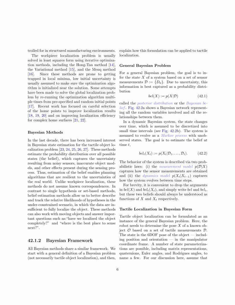
object pose. Fig. 42.6 shows examples of the effect ofdifferent actions on different beliefs.

Based on the possible object poses according to thecurrent belief belt, we need to consider the possibleoutcomes of each action A. However, the same actioncan result in different outcomes depending on the ac-tual object pose, which is not known to us exactly.

Simulation Experiments Since we can not deter-mine the effect of action A exactly, we approximateit by performing a series of simulation experiments.Let Xt be the current set of state hypotheses. Forhistogram filters, this can be the entire set X . Forparticle filters, it is the current set of particles. Foreach particular object pose X ∈ Xt, we can use a ge-ometric simulation to determine where the hand willstop along a guarded motion A, and what observa-tion D we are likely to see. Then, we can performa Bayesian update of belt to obtain simulated belief

belA,D that would result if we chosen action A andobserved D. Let DA denote the set of all simulatedobservations we obtained for an action A using theseexperiments.

To completely account for all possible outcomes,we need to simulate all possible noisy executions ofaction A and all possible resulting noisy observationsD. However, restricting our consideration to the setof noise-free simulations works well in practice.

Each action A may also have an associated costC(A,D), which represents how expensive or risky itis to execute A. Note, that the action cost may de-pend on the observation D. For example, if the costis the amount of time it takes to execute A, thendepending on where the contact is sensed, the sameguarded motion will stop at a different time along thetrajectory.

Utility Function In order to decide which actionto take, we need a utility function U(A) that allowsus to compare different possible actions. The utilityfunction should take into account both the usefulnessof the action as well as its cost.

To localize the object, we want to reduce the un-certainty about its pose. Hence, we can measure ac-tion usefulness in terms of uncertainty of the result-

ing belief. Intuitively, the lower the uncertainty, thehigher the usefulness of an action. The amount of un-certainty in a belief can be measured using entropy ,which for a probability distribution q(X) is definedas

H(q) := −∫q(X) log q(X) dX. (42.11)

For each simulated belief belA,D, we define its util-ity to be a linear combination of its usefulness (i.e.,certainty) and cost

U(belA,D) := −H(belA,D)− β C(A,D), (42.12)

where β is a weight that trades off cost and usefulness[39]. Since we do not know what observation we willget after executing action A, we define its utility tobe the expected utility of the resulting belief basedon all possible observations

U(A) := ED[U(belA,D)

]. (42.13)

Based on the simulation experiments, this expecta-tion can be estimated as a weighted sum over all theexperiments

U(A) ≈∑D∈DA

wD U(belA,D), (42.14)

where the weight wD is the probability of the state Xthat was used to generate the observation D. Morespecifically, for a grid representation of state space,each D ∈ DA was generated using some X ∈ Xt, andthus, wD is the belief estimated for the grid pointX. If Xt is represented by a set of weighted particles,then wD is the weight of particle X ∈ Xt used togenerate the observation D.

With this utility function in mind, the best actionto execute is the one with the highest utility

Abest := argmaxA

[U(A)

]. (42.15)

Since the utility function depends on negative en-tropy, methods that maximize this utility functionare often called entropy minimization methods.

15

Figure 42.6: Selecting an action using a KLD-basedutility function on examples of localizing a door handle.For each example, the starting belief belt is shown on theleft. The action chosen A := abest and the resulting beliefbelt+1 after executing the action are shown on the right.Color shows the probability of the state, ranging fromhigh (red) to low (blue) [39].

Alternative Utility Measures Other measures ofusefulness are also possible, such as reduction in av-erage variance of the belief or Kullback-Leibler diver-gence (KLD) of the simulated belief from the currentbelief. However, KLD is only applicable for problemswhere the object is stationary as this metric does notsupport a changing state. An example of action se-lection using KLD metric is shown in Fig. 42.6.

If the goal is to successfully grasp the object, notjust to localize it, then it makes more sense to se-lect actions that maximize probability of grasp suc-cess rather than simply minimizing entropy. Successcriteria for grasping can, for instance, be expressedgeometrically as ranges in particular dimensions ofobject pose uncertainty that are required for a task tosucceed. For a given belief, we can add up the proba-bilities corresponding to the object poses (states) forwhich executing a desired, task-directed grasp wouldsucceed open-loop, and maximize that value ratherthan minimizing entropy. Action selection can stillbe done using one-step-lookahead. Using this met-ric instead of the one in (42.12) simply allows one toconcentrate on reducing uncertainty along importantdimensions, while paying less attention to unimpor-tant dimensions [42]. For example, the axial rotation

of a nearly-cylindrical object is unimportant if it onlyneeds to be grasped successfully.

Multi-step planning in belief space

While in some situations one-step-lookahead meth-ods give good results, in other situations it may beadvantageous to look more than one step ahead. Thisis especially true if actions take a long time to exe-cute, and/or if the plan can be stored and re-used formultiple manipulation attempts.

Multi-step lookahead can be performed by con-structing a finite-depth search tree (see Fig. 42.7 forillustration). Starting with the current belief belt,we consider possible first-step actions A1, . . . , A3 andsimulate observations D11, . . . , D32. For each simu-lated observation, we perform a belief update to ob-tain the simulated beliefs B11, . . . , B32. For each ofthese simulated beliefs, we consider possible second-step actions (of which only A4, . . . , A6 are shown).For each of the second-step actions, we again simulateobservations and compute simulated beliefs. Thisprocess is repeated for third-step actions, fourth-stepactions, and so on, until the desired number of stepsis reached. The example in Fig. 42.7 shows the searchtree for two-step lookahead.

After the tree is constructed from the top down tothe desired depth, scoring is performed from the bot-tom up. Leaf beliefs are evaluated using the chosenutility metric. In the example in Fig. 42.7, the leafsshown are B41, . . . , B62. For each leaf, we show theentropy H and cost βC. The utility of each corre-sponding action A4, . . . , A6 is then computed by tak-ing expectation over all observations that were sim-ulated for that action. Note that we have to takeexpectations at this level because we have no controlover which of the simulated observations we will actu-ally observe. However, at the next level, we do havecontrol over which action to execute, and we selectthe action with the maximum utility [42]. We com-pute the utility of beliefs B11, . . . , B32 by subtractingtheir cost from the utility of the best action amongtheir children. For example,

U(B22) = U(A6)− βC(A2, D22). (42.16)

In this manner, expectation and maximization can be

16

Figure 42.7: Part of a depth-2 search tree through belief space, for three actions at each level and two canonicalobservations for each action. belt is the current belief. A1, . . . , A6 are actions. D11, . . . , D62 are simulated obser-vations. And B11, . . . , B62 are simulated beliefs. We can compute the entropy H and action cost β C at the leafs,and thus compute the utility metric U for each leaf. Then, working upwards from the bottom, we can compute theexpected utility U of actions A4, . . . , A6 by taking a weighted sum of their children. We then select the action withmaximum utility (A6 in this example) and use its utility U(A6) to compute the utility at node B22 using equation(42.16). The same operation is repeated for the upper levels, and at the top level we finally select the action withthe highest utility as the best action to be performed (A2 in this example) [42].

17

carried out for multiple levels of the tree until the topis reached. Maximization at the very top level selectsthe most optimum action to execute next. Bold linesin Fig. 42.7 show the possible action sequences thisalgorithm would consider optimal depending on thepossible observations made.

When searching to a depth greater than 1, branch-ing on every possible observation is likely to be pro-hibitive. Instead, we can cluster observations basedon how similar they are into a small number of canon-ical observations and only branch on these canonicalobservations.

Performing a multi-step search allows us to includeany desired final grasps as actions. These actions canresult in early termination if the success criterion ismet, but can also function as possible information-gathering actions if the criterion is not met. It alsoallows us to reason about actions that may be re-quired to make desired grasps possible, such as reori-enting the object to bring it within reach. As shownin [42], a two-step lookahead search is usually suffi-cient. Searching to a depth of 3 generally yields littleadditional benefit. One full sequence of information-gathering, grasping, and object reorientation using amulti-step search with a depth of 2 for grasping apower drill is shown in Fig. 42.8.

Other Planning Methods

There are many other possible methods for selectingactions while performing Bayesian state estimationfor tactile object localization and grasping. As longas we continue to track the belief with one of the infer-ence methods described above, even random actionscan make progress towards successfully localizing theobject. In this section, we will describe a few sig-nificantly different approaches to action selection forBayesian object localization.

The planning methods we have described so farused either guarded motions or move-until-contact,to avoid disturbing or knocking over the object. How-ever, one can instead use the dynamics of objectpushing to both localize and constrain the object’spose in the process of push-grasping, as in Dogar etal. [43].

Also, instead of using entire trajectories as actions,

Figure 42.8: An example sequence of grasping a power-drill based on a depth-2 search through belief space. Theright side of each pair of images shows the grasp just ex-ecuted, while the left side shows the resulting belief. Thedark blue flat rectangle and the red point-outline of thepowerdrill show the most likely state, while the light bluerectangles show states that are 1 standard deviation awayfrom the mean in each dimension (x, y, θ). Panels a-c ande-g show information-gathering grasps being used to lo-calize the drill, panel d shows the robot reorienting thedrill to bring the desired grasp within reach, and panelsh and i show the robot using the desired final grasp onthe drill, lifting, and pulling the trigger successfully. [42].

18

we could consider smaller motions as actions out ofwhich larger trajectories could be built. In this case,one- or two-step lookahead will be insufficient to getgood results. Instead, we would need to constructplans consisting of many steps. In other words, wewould need a much longer planning horizon. Thechallenge is that searching through belief space asdescribed above is exponential in the planning hori-zon. In Platt et al. [44], the authors get around thisproblem by assuming the current most likely state istrue and searching for longer-horizon plans that willboth reach the goal and also differentiate the currentmost likely hypothesis from other sampled, compet-ing states. If we monitor the belief during executionand re-plan whenever it diverges by more than a setthreshold, the goal will eventually be reached becauseeach hypothesis will be either confirmed (and thus thegoal reached) or disproved.

Finally, while the above methods can be used forplanning for what we termed global localization (i.e.,object localization under high uncertainty), if the ob-ject needs to be localized in an even broader context,as when trying to locate an object somewhere in akitchen, then one may have to plan to gather infor-mation with higher-level actions (e.g., opening cab-inets). Such actions could be reasoned about usingsymbolic task planning, as in Kaelbling and Lozano-Perez [45].

42.2 Learning About An Ob-ject

While the previous section focused on localization ofknown objects, in this section, we discuss methodsfor learning about a previously unknown object orenvironment. The goal is to build a representationof the object that can later be useful for localiza-tion, grasp planning, or manipulation of the object.A number of properties may need to be estimated,including shape, inertia, friction, contact state, andothers.

42.2.1 Shape of Rigid Objects

In this set of problems, the goal is to construct a 2D or3D model of the object’s geometric shape by touchingthe object. Due to low data acquisition rate, touch-based shape reconstruction faces special challengesas compared to methods based on dense 3D camerasor scanners. These challenges dictate the choice ofobject representation and exploration strategy.

While most of the work on shape reconstruction fo-cuses on poking motions with the end-effector, somemethods rely on techniques such as rolling the objectin between planar palms equipped with tactile sen-sors. In these methods, shape of the object can bereconstructed from the contact curves traced out bythe object on the palms. These methods were firstdeveloped for planar 2D objects [46], and later ex-tended to 3D [47].

Representation

The shape reconstruction process is heavily depen-dent on the chosen representation. Since the dataare sparse, a simpler shape representation can signif-icantly speed up the shape acquisition process.

Shape Primitives The simplest representation isa primitive shape: plane, sphere, cylinder, torus,tetrahedra, or cube. In this case, only a few pa-rameters need to be estimated based on the gathereddata. For example, Slaets et al. estimate the size of acube by performing compliant motions with the cubepressed against a table [49].

Patchwork of Primitives If one primitive doesnot describe the whole object well, a “patchwork” ofseveral primitives may be used. Parts of the objectare represented with sub-surfaces of different primi-tives, which are fused together [48] (see Fig. 42.9). Inthis case, a strategy for refining the fusion boundariesbetween primitives is needed and additional data maybe gathered for this specific purpose.

Super-quadrics A slightly more complex primi-tive shape is a super-quadric surface, which gives

19

Figure 42.9: A combination of primitive shapes and polygonal mesh is used for modeling objects during an under-water mapping experiment [48].

more flexibility than a simple primitive. Super-quadric surfaces are surfaces described in sphericalcoordinates by

S(ω1, ω2) :=

cx cosε1 (ω1) cosε2 (ω2)cy cosε1 (ω1) sinε2 (ω2)

cz sinε1 (ω1)

. (42.17)

The parameters cx, cy, and cz describe the extent ofthe super-quadric along the axes x, y, and z respec-tively. By adjusting the exponents ε1 and ε2, one canvary the resulting shape anywhere from an ellipse toa box. For example, setting ε1, ε2 ≈ 0 results in boxshapes; ε1 = 1, ε2 ≈ 0 results in cylindrical shapes;ε1, ε2 = 1 results in ellipses. Hence, by estimatingcx, cy, cz, ε1, and ε2, one can model a rich variety ofshapes [50].

Polygonal Mesh When none of the paramet-ric representations capture the object’s shape wellenough, a polygonal mesh can be used. A polygonalmesh (or poly-mesh) can represent arbitrary shapesas it consists of polygons (typically, triangles) linkedtogether to form a surface (Fig. 42.1). The simplestmethod is to link up collected data points to create

faces (i.e., the polygons) of the mesh. However, thismethod tends to under-estimate the overall size ofthe object because data points at object corners arerarely gathered. This effect is present even for dense3D sensors, but especially noticeable here due to spar-sity of the data. A more accurate representation canbe obtained by collecting several data points for eachpolygonal face and, then, intersecting the polygonalfaces to obtain the corners of the mesh. However, thistends to be a more involved, manual process [28].

Point Cloud Objects can also be represented asclouds of gathered data points. In this case, theaccuracy of the representation directly depends onthe density of the gathered data and, hence, thesemethods typically spend a lot of time collecting data[51, 52].

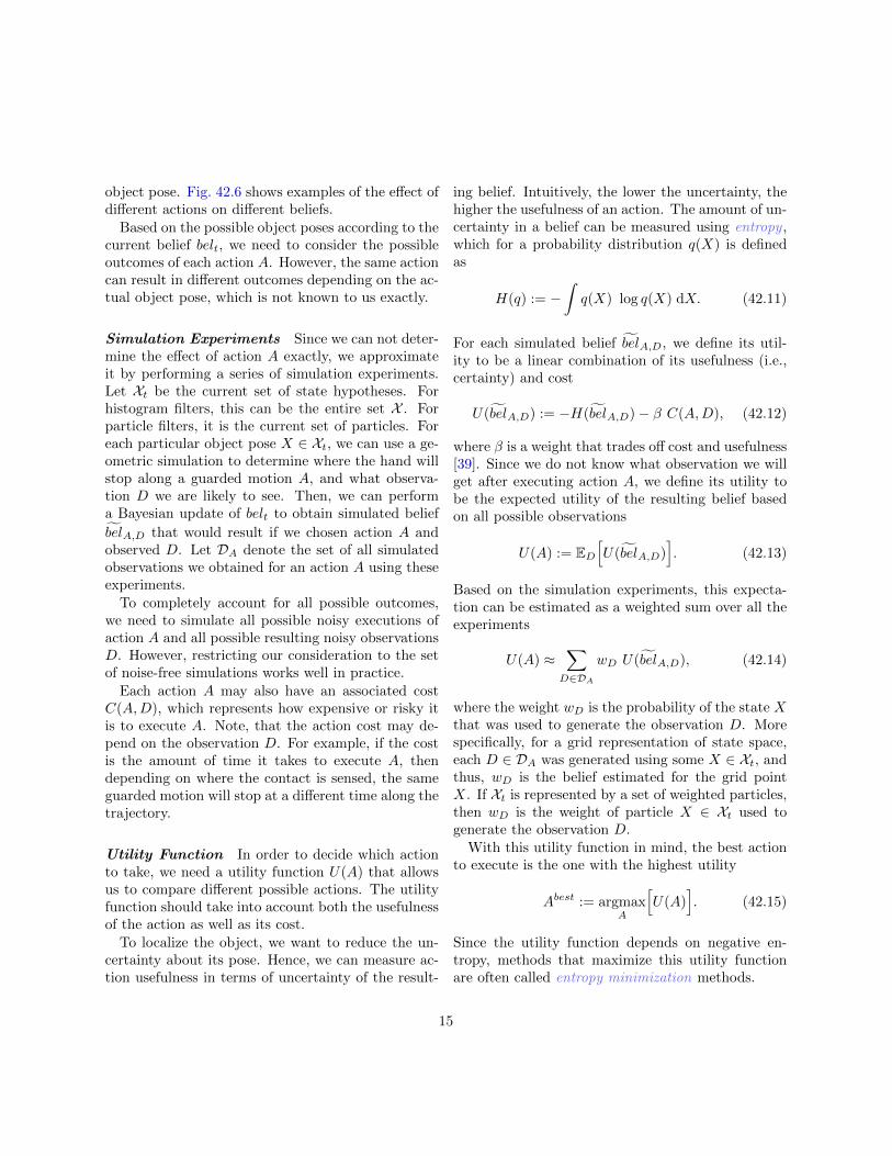
Splines 2D objects can be represented by splines.For example, Walker and Salisbury used proximitysensors and a planar robot to map smooth shapesplaced on a flat surface [53] (Fig. 42.10).

20

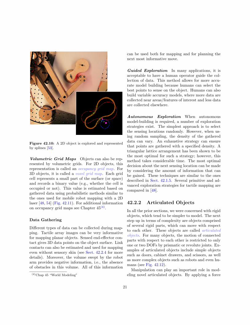
Figure 42.10: A 2D object is explored and representedby splines [53].

Volumetric Grid Maps Objects can also be rep-resented by volumetric grids. For 2D objects, thisrepresentation is called an occupancy grid map. For3D objects, it is called a voxel grid map. Each gridcell represents a small part of the surface (or space)and records a binary value (e.g., whether the cell isoccupied or not). This value is estimated based ongathered data using probabilistic methods similar tothe ones used for mobile robot mapping with a 2Dlaser [48, 54] (Fig. 42.11). For additional informationon occupancy grid maps see Chapter 45(4).

Data Gathering

Different types of data can be collected during map-ping. Tactile array images can be very informativefor mapping planar objects. Sensed end-effector con-tact gives 3D data points on the object surface. Linkcontacts can also be estimated and used for mappingeven without sensory skin (see Sect. 42.2.4 for moredetails). Moreover, the volume swept by the robotarm provides negative information, i.e., the absenceof obstacles in this volume. All of this information

(4)Chap 45 “World Modeling”

can be used both for mapping and for planning thenext most informative move.

Guided Exploration In many applications, it isacceptable to have a human operator guide the col-lection of data. This method allows for more accu-rate model building because humans can select thebest points to sense on the object. Humans can alsobuild variable accuracy models, where more data arecollected near areas/features of interest and less dataare collected elsewhere.

Autonomous Exploration When autonomousmodel-building is required, a number of explorationstrategies exist. The simplest approach is to selectthe sensing locations randomly. However, when us-ing random sampling, the density of the gathereddata can vary. An exhaustive strategy can ensurethat points are gathered with a specified density. Atriangular lattice arrangement has been shown to bethe most optimal for such a strategy; however, thismethod takes considerable time. The most optimaldecision about the next sensing location can be madeby considering the amount of information that canbe gained. These techniques are similar to the onesdescribed in Sect. 42.1.5. Several primitive and ad-vanced exploration strategies for tactile mapping arecompared in [48].

42.2.2 Articulated Objects

In all the prior sections, we were concerned with rigidobjects, which tend to be simpler to model. The nextstep up in terms of complexity are objects comprisedof several rigid parts, which can move with respectto each other. These objects are called articulatedobjects. For many objects, the motion of connectedparts with respect to each other is restricted to onlyone or two DOFs by prismatic or revolute joints. Ex-amples of articulated objects include simple objectssuch as doors, cabinet drawers, and scissors, as wellas more complex objects such as robots and even hu-mans (see Fig. 42.12).

Manipulation can play an important role in mod-eling novel articulated objects. By applying a force

21

Figure 42.11: Reconstruction of letters from tactile images. Pixels are colored by probability of occupancy inlog-odds form. This probability can be seen to be high on the letters themselves, to be low in the surrounding areawhere measurements were taken, and to decay to the prior probability in the surrounding un-sensed area [54].

Figure 42.12: Robot manipulating a variety of common articulated objects (from left to right): a cabinet door thatopens to the right, a cabinet door that opens to the left, a dishwasher, a drawer, and a sliding cabinet door [55].

Figure 42.13: Robot exploring an articulated object[57].

to one part of an articulated object, one can observehow the other parts move and thus infer relation-ships between parts. Observation can be performedvia the sense of touch or via some other sense, e.g.,vision. For example, if a robot arm pulls/pushes adoor compliantly, its trajectory allows the robot todetermine the width of the door [56]. Alternatively,if a robot arm pushes one handle of a pair of scis-sors, the location of the scissors joint can be inferredby tracking visual features with an overhead camera(see Fig. 42.13).

A kinematic structure consisting of several revo-

lute and prismatic joints can be represented as a re-lational model , which describes relationships betweenobject parts. In order to build a relational model ofa multi-joint object, a robot needs an efficient explo-ration strategy for gathering the data. The explo-ration task can be described using a Markov decisionprocess, similar to the ones discussed in Sect. 42.1.5.Since the goal is to learn relational models, theseMDPs are called relational Markov decision processes(RMDPs). With the aid of RMDPs, robots can learnefficient strategies for exploring previously unknownarticulated objects, learning their kinematic struc-ture, and later manipulating them to achieve the goalstate [57].

Some kinematic structures do not consist entirelyof revolute and prismatic joints. A common exam-ple is garage doors, which slide in and out along acurved trajectory. General kinematic models can berepresented by Gaussian processes, which can cap-ture revolute, prismatic and other types of connec-tions between parts [55].

22

Figure 42.14: Robot exploring a 2D deformable object[59].

Figure 42.15: Model of a 3D deformable object. Theobject at rest (left). The object under influence of anexternal force (center and right). Images are from [60].

42.2.3 Deformable Objects

Even more complex than articulated objects are de-formable objects, which can be moved to form ar-bitrary shapes. The simplest of these are 1-D de-formable objects, such as ropes, strings, and ca-bles. These objects are typically modeled as line ob-jects with arbitrary deformation capability (exceptfor stretching). A number of approaches can be foundin [58].

A more complex type of deformable objects are pla-nar deformable objects, such as fabric or deformableplastic sheets. While these objects can be repre-sented as networks of nodes, modeling interactionbetween these nodes can get expensive and is not al-ways necessary. For example, Platt et al. developed

an approach to mapping planar deformable objectsby swiping them between the robot’s fingers [59] (seeFig. 42.14). These maps can later be used for local-ization during subsequent swipes, in a manner similarto indoor robot localization on a map.

The most complex deformable objects are 3D de-formable objects. This category includes a great vari-ety of objects in our everyday environments: sponges,sofas, and bread are just a few examples. Moreover,in medical robotics, tissues typically have to be mod-eled as 3D deformable objects. Since the stiffness andcomposition of these objects can vary, they need to bemodeled as networks of nodes, where different inter-action can take place between distinct nodes. Suchmodels typically require a lot of parameters to de-scribe even reasonably small objects. Although, someefficiency improvements can be obtained by assumingthat subregions of the object have similar properties.Despite the challenges, 3D deformable object model-ing has many useful applications, e.g., a surgery sim-ulator or 3D graphics. Burion et al. modeled 3D ob-jects as a mass-spring system (see Fig. 42.15), wheremass nodes are inter-connected by springs [60]. Byapplying forces to the object, one can observe the de-formation and infer stiffness parameters of the springs(i.e., elongation, flexion, and torsion).

42.2.4 Contact Estimation

Up until now, we have assumed that the contact lo-cation during data gathering was somehow known.However, determining the contact point is not asstraightforward for robots as it is for humans, be-cause robots are not fully covered in sensory skin.Thus, during interaction between a robot and its en-vironment, non-sensing parts of the robot can comein contact with the environment. If such contact goesundetected, the robot and/or the environment maybe damaged. For this reason, touch sensing is typi-cally performed by placing sensors at the end-effectorand ensuring that the sensing trajectories never bringnon-sensing parts of the robot in contact with the en-vironment.

Clearly, end-effector-only sensing is a significantconstraint, which is difficult to satisfy in real-worldconditions. Work on whole-body sensory skin is ongo-

23

ing [61], yet for now only small portions of the robot’ssurface tend to be covered with sensory skin.

In lieu of sensory skin, contact can be estimatedfrom geometry of the robot and the environment viaactive sensing with compliant motions. Once a con-tact between the robot and the environment is de-tected (e.g., via deviation in joint torques or angles),the robot switches to the active sensing procedure.During this procedure, the robot performs compliantmotions (either in hardware or software), by applyinga small force towards the environment and movingback and forth. Intuitively, the robot’s body carvesout free space as it moves, and thus, via geometricalreasoning, the shape of the environment and contactpoints can be deduced. However, from a mathemat-ical perspective, this can be done in several differentways.

One of the earliest approaches was developedby Kaneko et al., who formulated the Self-PostureChangability (SPC) method [63]. In SPC, the inter-section of finger surfaces during the compliant mo-tions is taken to be the point of contact. This methodworks well in areas of high curvature of the environ-ment (e.g., corners), but can give noisy results in ar-eas of shallow curvature. In contrast to SPC, theSpace Sweeping algorithm by Jentoft et al. marksall points on finger surfaces as possible contact, andthen gradually rules out the possibilities [62] (seeFig. 42.16). The Space Sweeping algorithm providesless noisy estimates in areas of shallow curvature, butcan be more susceptible to even the smallest distur-bances of the environment’s surface.

Mathematically, contact estimation can also be for-mulated as a Bayesian estimation problem. If therobot moves using compliant motions as describedabove, the sensor data are the joint angles of therobot. The state is the shape and position of the en-vironment, represented using one of the rigid objectmodels described in Sect. 42.2.1. Then, each pos-sible state can be scored using a probabilistic mea-surement model, e.g., the proximity model describedin Sect. 42.1.2, and the problem can be solved usingBayesian inference methods [64].

(a)

(b)

Figure 42.16: (a) A two-link compliant finger used forcontact sensing. (b) The resulting model built by theSpace Sweeping algorithm. Images are from [62].

24

42.2.5 Physical Properties

Up until now, we have focused on figuring out theshape and articulation of objects. While there aresome advantages to doing so with tactile data as op-posed to visual data, visual data can also be used togenerate shape and articulation models. However,there are many properties of objects that are noteasily detectable with vision alone, such as surfacetexture and friction, inertial properties, stiffness, orthermal conductivity.

Friction and Surface Texture

Surface friction, texture, and roughness can be esti-mated by dragging a fingertip over the object. Theforces required to drag a fingertip over a surface atdifferent velocities can be used to estimate surfacefriction parameters [65, 66, 67]. Accelerometer orpressure data is useful for estimating surface rough-ness (by the amplitude and frequency of vibrationwhile sliding) [67, 68], or more directly identifyingsurface textures using classification techniques suchas SVMs or k-NN [69]. The position of the fingertipbeing dragged across the surface is also useful for esti-mating surface roughness and for mapping out smallsurface features [65]. Static friction is also often esti-mated as a by-product of trying to avoid object slipduring a grasp, based on the normal force being ap-plied at the moment when slip happens [70, 71]. Fi-nally, the support friction distribution for an objectsliding on a surface can be estimated by pushing theobject at different locations and seeing how it moves[53, 72].

Inertia

Atkeson et al. [73] estimate the mass, center of mass,and moments of inertia of a grasped object, usingmeasurements from a wrist force-torque sensor. Ob-jects that are not grasped but that are sitting on atable can be pushed; if the pushing forces at the fin-gertips are known, the object’s mass as well as theCOM and inertial parameters in the plane can beestimated. Yu et al. [74] do so by pushing objectsusing two fingertips equipped with force/torque sen-sors and recording the fingertip forces, velocities, and

accelerations. Tanaka et al. [75] estimate the object’smass by pushing the object with known contact forceand watching the resulting motion with a camera.

Stiffness

Identifying the stiffness (or the inverse, compliance)of an object is useful in terms of modeling the ma-terial properties of an object, but more directly, itis also useful for preventing the robot from crushingor damaging delicate objects. Gently squeezing anobject and measuring the deflection seen for a givencontact normal force is one method often used to es-timate stiffness [76, 77, 68]. Omata et al. [78] usea piezoelectric transducer and a pressure sensor ele-ment in a feedback circuit that changes its resonantfrequency upon touching an object, to estimate theobject’s acoustic impedance (which varies with bothobject stiffness and mass). Burion et al. [60] use par-ticle filters to estimate the stiffness parameters of amass-spring model for deformable objects, based onthe displacements seen when applying forces to dif-ferent locations on the object.

Thermal Conductivity

Thermal sensors are useful for identifying the ma-terial composition of objects based on their thermalconductivity. Fingertips with internal temperaturesensors [79, 68] can estimate the thermal conductiv-ity of the object by heating a robot fingertip to aboveroom temperature, touching the fingertip to the ob-ject, and measuring the rate of heat loss.

42.3 Recognition

Another common goal of touch-based perception isto recognize objects. As with more typical, vision-based object recognition, the goal is to identify theobject from a set of possible objects. Some methodsassume known object shapes and try to figure outwhich object geometry matches the sensor data best.Other methods use feature-based pattern recognitionto identify the object, often with a bag-of-featuresmodel that does not rely on geometric comparisons tooverall object shape. Finally, there are methods that

25

use object properties such as elasticity or texture toidentify objects.

42.3.1 Object shape matching

Any of the methods for shape-based localization canalso be used for recognition, by performing localiza-tion on all potential objects. In terms of the equa-tions used in Sect. 42.1, if we are considering a limitednumber of potential objects with known mesh mod-els, we can simply expand our state space to includehypotheses over object identity and pose, instead ofjust pose. If we add an object ID to each state in thestate vector X, and use the appropriate mesh modelfor that object ID for the measurement model foreach state, all of the equations used in the previoussections still hold. The object ID for the combinedobject shape and pose that best matches the collectedsensor data is then our top object hypothesis.

Non-probabilistic methods for localization and ob-ject recognition often involve geometrically pruningobjects from a set of possible object shapes/posesthat do not match sensed data. For instance, Gastonet al. [80] and Grimson et al. [81] recognize and lo-calize polyhedral objects by using the positions andnormals of sensed contact points in a generate-and-test framework: generate feasible hypotheses aboutpairings between sensed contact points and objectsurfaces, and test them for consistency based on con-straints over pairs of sensed points and their hypoth-esized face locations and normals. Russell et al [82]classify tactile array images as point, line, or areacontacts, and use the time-sequence of contacts seenwhen rolling the object over the array to prune in-consistent object shapes.

Other methods recognize objects by forming amodel of the object, then matching the new modelwith database objects. For instance, Allen andRoberts [83] build superquadric models of the objectfrom contact data, then match the superquadric pa-rameters against a database of object models. Caselliet al. [84] build polyhedral representations of objects(one based on contact points and normals that rep-resents the space that the true object must fit inside,and one based on just contact points that the trueobject must envelop), and use the resulting represen-

tations to prune incompatible objects in a databaseof polyhedral objects.

42.3.2 Statistical pattern recognition

Many methods for tactile object recognition use tech-niques from statistical pattern recognition, summa-rizing sensed data with features and classifying theresulting feature vectors to determine the identity ofthe object. For instance, Schopfer et al. [85] roll atactile array over objects along a straight line, com-pute features such as image blob centroids and secondor third moments over the resulting time series of tac-tile images, and use a decision tree to classify objectsbased on the resulting features. Bhattacharjee et al.[86] use k-nearest-neighbors on a set of features basedon time series images from a forearm tactile array toidentify whether an object is fixed or movable, andrigid or soft, in addition to recognizing the specificobject.

Tactile array data is very similar to small imagepatches in visual data, and so techniques for objectrecognition using tactile arrays can look much likeobject recognition techniques that use visual data.For instance, Pezzementi et al. [88] and Schneideret al. [87] both use a Bag-of-Features model on fin-gertip tactile array data to recognize objects. Theprocess for tactile data is almost the same as for vi-sual images: for each training object (image), a set oftactile array images (2D image patches) is obtained(for an example, see Fig. 42.17), features (which arevectors of descriptive statistics) based on each tactileimage are computed, and the features for all objectsin the training set are clustered to form a vocabularyof canonical features (see Fig. 42.18). Each object isrepresented as a histogram of how often each featureoccurs. When looking at a new, unknown object, thefeatures computed from the tactile array images aresimilarly used to compute a histogram, and then thenew histogram is compared against those of the ob-jects in the database to find the best match. Theone notable difference in the two domains is that tac-tile data is much more time-consuming and difficultto obtain than appropriate image patches: in 2D vi-sual object recognition, an interest point detectionalgorithm can quickly produce hundreds of salient

26

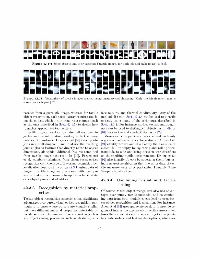
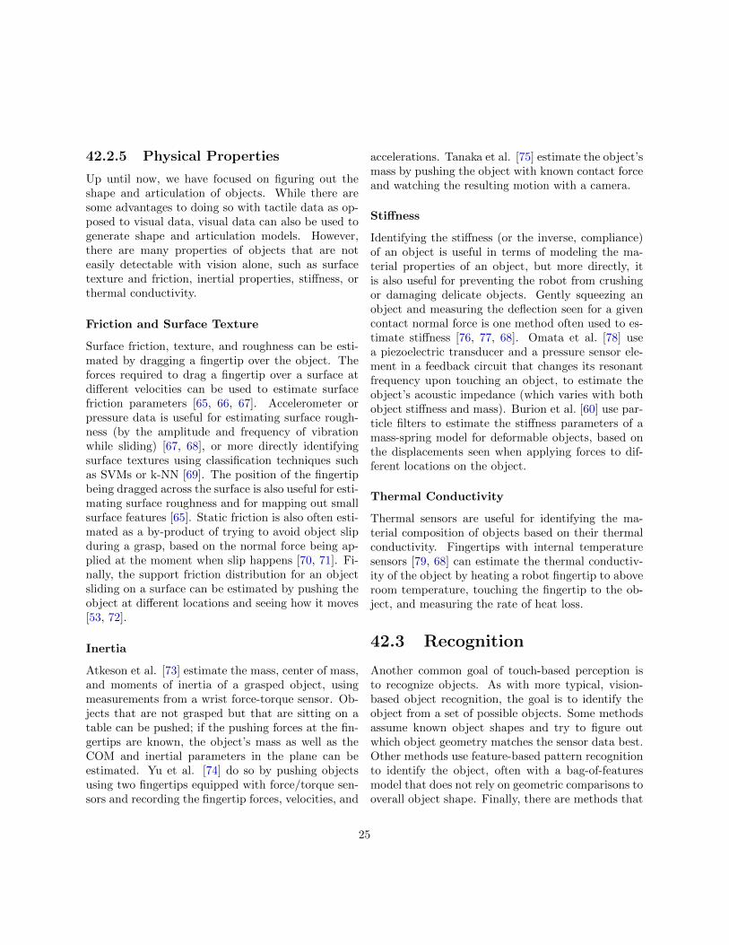
Figure 42.17: Some objects and their associated tactile images for both left and right fingertips [87].

Figure 42.18: Vocabulary of tactile images created using unsupervised clustering. Only the left finger’s image isshown for each pair [87].

patches from a given 2D image, whereas for tactileobject recognition, each tactile array requires touch-ing the object, which in turn requires a planner (suchas the ones described in Sect. 42.1.5) to decide howto gather appropriate tactile data.

Tactile object exploration also allows one togather and use information besides just tactile imagepatches: for instance, Gorges et al [89] envelop ob-jects in a multi-fingered hand, and use the resultingjoint angles as features that directly relate to objectdimensions, alongside additional features computedfrom tactile image patterns. In [90], Pezzementiet al. combine techniques from vision-based objectrecognition with the type of Bayesian recognition-by-localization described in section 42.3.1, using pairs offingertip tactile image features along with their po-sitions and surface normals to update a belief stateover object poses and identities.

42.3.3 Recognition by material prop-erties

Tactile object recognition sometimes has significantadvantages over purely visual object recognition, par-ticularly in cases where objects are visually similarbut have different material properties detectable bytactile sensors. A number of recent methods clas-sify objects using properties such as elasticity, sur-

face texture, and thermal conductivity. Any of themethods listed in Sect. 42.2.5 can be used to identifyobjects, using many of the techniques described inSect. 42.3.2. For instance, surface texture and rough-ness can be used to distinguish objects, as in [69] or[67], as can thermal conductivity, as in [79].

More specific properties can also be used to classifyobjects of particular types: for instance, Chitta et al.[91] identify bottles and also classify them as open orclosed, full or empty by squeezing and rolling themfrom side to side and using decision tree classifierson the resulting tactile measurements. Drimus et al.[92] also identify objects by squeezing them, but us-ing k-nearest neighbor on the time series data of tac-tile measurements after performing Dynamic TimeWarping to align them.

42.3.4 Combining visual and tactilesensing

Of course, visual object recognition also has advan-tages over purely tactile methods, and so combin-ing data from both modalities can lead to even bet-ter object recognition and localization. For instance,Allen et al [93] uses sparse stereo data to provide re-gions of interest to explore with tactile sensors, thenfuses the stereo data with the resulting tactile pointsto create surface and feature descriptions, which are

27

then matched against objects in the database; ob-ject hypotheses are further verified with tactile explo-ration. Boshra and Zhang [94] recognize polyhedralobjects by using tactile features and visual verticesand edges to formulate constraints in a constraint-satisfaction problem. Nakamura et al. [95] graspobjects and learn object categories based on visualdata (in the form of SIFT descriptors), audio infor-mation obtained while shaking (using a codebookof audio features based on Mel-frequency cepstralcoefficients), and haptic information obtained whilesqueezing (using hardness estimates based on fingerpressure sensor readings); the learning and inferenceare done using probabilistic Latent Semantic Analy-sis (pLSA).

Segmenting an object from a visual scene (whichmakes further efforts at recognition much easier) isalso made easier by combining visual and tactilesensing; by pushing on an object and seeing whichparts of the visual scene move together, objects canbe segmented both from the background and fromeach other. For instance, Gupta and Sukhatme [96]use RGB-D data along with manipulation primitivessuch as spreading motions to segment and sort Duplobricks, and Hausman et al. [97] segment texturelessobjects in RGB-D data by performing visual segmen-tation and then resolving ambiguities using pushingmotions.

Work on categorizing objects by their affordancesor functions often also uses both visual and tactiledata. For instance, Sutton [98] uses both shape-basedreasoning (using shape derived from range images) aswell as interaction-based reasoning (using data fromthe robot physically interacting with the object) topredict and confirm object affordances such as grasp-ing, containing, and sitting (being suitable for hu-mans to sit upon). Bekiroglu [99] performs inferenceon a Bayesian Network using visual, proprioceptive,and tactile data to assess whether an object/graspcombination will be both stable and also good for atask such as pouring, hand-over, or dishwashing.

42.4 Conclusions

This chapter described perceptual methods that relyon manipulation. Although these methods are gener-ally more complex than vision-based perception, theyare useful in low-visibility conditions, in determiningproperties that require manipulation, and in situa-tions where perception is needed for subsequent ma-nipulation tasks. Perception-via-manipulation facesspecial challenges due to the low data acquisition rateand the fact that each sensing action disturbs thescene. To address these challenges, special inferencemethods have been developed to cope with situationswhere data are insufficient to fully constrain the prob-lem (Sect. 42.1.3). Special planning methods had tobe applied to minimize the number of sensing actionsand reduce the possibility of significant scene distur-bance or non-sensed contacts (Sect. 42.1.5). Thesechallenges also dictate the choice of object models(Sect. 42.2), and play a role in object recognitionmethods (Sect. 42.3).

42.4.1 Real-Life Applications

Perception-via-manipulation is already used in anumber of real-world applications and an even greaternumber of applications will likely benefit from it inthe near future. In manufacturing, touch-based lo-calization of parts for machining or assembly is oftenpreferred to optical methods because it is not affectedby optical properties of objects (e.g., transparency orreflectivity). At present, low uncertainty in part po-sitioning is required prior to touch-based localization,which leads to high instrumentation and reconfigura-tion costs. However, the new localization methodspresented in this chapter can cope with high uncer-tainty and thus enable flexible manufacturing linescapable of producing a variety of parts without recon-figuration. In the future, fully-automated in-homemanufacturing may even become possible.

Medical robotics is another mature real-world ap-plication, in which robotic contact with the environ-ment (i.e., the patient) is not only unavoidable, it isin fact required for many of the procedures. Visibil-ity is often poor, and sensing with devices that emitsound, light, or other waves can be harmful to the

28

patient. Under these conditions, sensing-via-contactcan sometimes be the most viable option. The envi-ronment is inherently deformable, and thus, medicalrobotics has been a strong driver for research on ma-nipulation and perception of deformable objects.

Another area in which robots are indispensable isunderwater robotics. It is not always safe or con-venient for humans to be performing tasks deep un-derwater, and hence, remotely-operated robots (orROV s) are a natural choice. ROVs even made inter-national news during recovery operations from theBP oil spill disaster in the Spring of 2010. Sincevisibility underwater is often poor, perception-via-contact plays an even more important role.

Beyond the more established robotic applications,as the fields of service robotics and disaster recoverydevelop, the necessity of sensing-via-contact becomesmore and more obvious. In these applications, robotsoften have to work in clutter and in close proximityto humans. Under these conditions, visibility can bepoor, yet at the same time, unsensed contact can bedisastrous.

42.4.2 Future Directions of Research

Inspired by the many existing and potential appli-cations, the field of perception-by-manipulation isevolving and receiving more attention. Despite thechallenges, there are bountiful opportunities for fur-ther fruitful research.

• The vast majority of touch-based perceptionwork deals with rigid objects, whereas many ob-jects in our environments are articulated and/ordeformable. These types of objects need to bestudied in more detail.

• For rigid objects, touch-based perception of mov-ing objects, object piles, and objects in clutterhas been under-explored.

• Whole-body contact estimation needs further at-tention, with or without sensory skin. The chal-lenges here are significant, but good solutionswould increase the safety of robots in service ap-plications and other unstructured environments.

• Last but not least, while Bayesian methods havefound wide acceptance in other areas of robotics,touch-based perception has yet to fully bene-fit from these methods. Thus, application ofBayesian methods to any of the above listed ar-eas is particularly promising.

42.4.3 Further Reading

For a broader view, a lot of related material can befound in other chapters throughout this handbook.Most sensing-via-manipulation is done using contactor near-contact (i.e., close-range) sensors. These sen-sors are described in Chapter 28(5). A few approachesuse classical vision sensors in conjunction with ma-nipulation (as in Sect. 42.2.2, for example). Visionsensors and methods are covered in Chapters 32(6)

and 34(7). Manipulator design and control are cov-ered in Chapters 4(8), 8(9), and 9(10). Other rele-vant chapters include 7(11), 14(12) and 47(13) for plan-ning methods, 37(14), 45(15), and 46(16) for modeling,33(17) for recognition, 5(18) and 35(19) for inference.

(5)Chap 28 “Force and Tactile Sensing”(6)Chap 32 “3D Vision”(7)Chap 34 “Visual Servoing and Visual Tracking”(8)Chap 4 “Mechanisms and Actuation”(9)Chap 8 “Motion Control”

(10)Chap 9 “Force Control”(11)Chap 7 “Motion Planning”(12)Chap 14 “AI Reasoning Methods for Robotics”(13)Chap 47 “Motion Planning and Obstacle Avoidance”(14)Chap 37 “Contact Modeling and Manipulation”(15)Chap 45 “World Modeling”(16)Chap 46 “SLAM”(17)Chap 33 “Object Recognition”(18)Chap 5 “Sensing and Estimation”(19)Chap 35 “Multisensor Data Fusion”

29

Bibliography

[1] P. C. Gaston and T. Lozano-Perez, “Tactilerecognition and localization using object mod-els,” tech. rep., MIT, AIM-705, 1983.

[2] W. E. L. Grimson and T. Lozano-Perez, “Model-based recognition and localization from sparserange or tactile data,” Journal of Robotics Re-search, 1983.

[3] O. Faugeras and M. Hebert, “A 3-d recogni-tion and positioning algorithm using geometricalmatching between primitive surfaces.,” in EighthIntl. Joint Conf. on Artificial Intelligence, LosAltos, CA, pp. 996–1002, 1983.

[4] S. Shekhar, O. Khatib, and M. Shimojo, “Sen-sor fusion and object localization,” in Proc. ofICRA, 1986.

[5] Y.-B. Jia and M. Erdmann, “Pose from push-ing,” in Proceedings of IEEE International Con-ference on Robotics and Automation, vol. 1,pp. 165–171, IEEE, 1996.

[6] K. Y. Goldberg, “Orienting polygonal partswithout sensors,” Algorithmica, vol. 10, no. 2-4, pp. 201–225, 1993.

[7] M. A. Erdmann and M. T. Mason, “An ex-ploration of sensorless manipulation,” Roboticsand Automation, IEEE Journal of, vol. 4, no. 4,pp. 369–379, 1988.

[8] H. Yau and C. Menq, “An automated di-mensional inspection environment for manufac-tured parts using coordinate measuring ma-chines,” International journal of production re-search, vol. 30, no. 7, pp. 1517–1536, 1992.

[9] K. Gunnarsson and F. Prinz, “CAD model-based localization of parts in manufacturing,”Computer;(United States), vol. 20, no. 8, 1987.

[10] K. Gunnarsson, Optimal part localization bydata base matching with sparse and dense data.PhD thesis, Dept. of Mechanical Engineering,Carnegie Mellon Univ., May 1987.

[11] H. Pahk and W. Ahn, “Precision inspection sys-tem for aircraft parts having very thin featuresbased on CAD/CAI integration,” The Interna-tional Journal of Advanced Manufacturing Tech-nology, vol. 12, no. 6, pp. 442–449, 1996.

[12] M. Cho and T. Seo, “Inspection planning strat-egy for the on-machine measurement processbased on CAD/CAM/CAI integration,” The In-ternational Journal of Advanced ManufacturingTechnology, vol. 19, no. 8, pp. 607–617, 2002.

[13] Z. Xiong, Workpiece Localization and ComputerAided Setup System. PhD thesis, The HongKong University of Science and Technology,2002.

[14] J. Hong and X. Tan, “Method and apparatus fordetermining position and orientation of mechan-ical objects,” May 4 1993. US Patent 5,208,763.

[15] B. Horn, “Closed-form solution of absolute ori-entation using unit quaternions,” JOSA A,vol. 4, no. 4, pp. 629–642, 1987.

[16] C. Menq, H. Yau, and G. Lai, “Automated pre-cision measurement of surface profile in CAD-directed inspection,” Robotics and Automation,IEEE Transactions on, vol. 8, no. 2, pp. 268–278, 1992.

30

[17] Y. Chu, Workpiece localization: Theory, algo-rithms and implementation. PhD thesis, TheHong Kong University of Science and Technol-ogy, 1999.

[18] Z. Xiong, M. Wang, and Z. Li, “A near-optimalprobing strategy for workpiece localization,”Robotics, IEEE Transactions on, vol. 20, no. 4,pp. 668–676, 2004.

[19] Y. Huang and X. Qian, “An Efficient Sensing Lo-calization Algorithm for Free-Form Surface Dig-itization,” Journal of Computing and Informa-tion Science in Engineering, vol. 8, p. 021008,2008.

[20] L. Zhu, H. Luo, and H. Ding, “Optimal Design ofMeasurement Point Layout for Workpiece Local-ization,” Journal of Manufacturing Science andEngineering, vol. 131, p. 011006, 2009.

[21] L. Zhu, Z. Xiong, H. Ding, and Y. Xiong, “Adistance function based approach for localizationand profile error evaluation of complex surface,”Journal of manufacturing Science and Engineer-ing, vol. 126, p. 542, 2004.

[22] Y. Sun, J. Xu, D. Guo, and Z. Jia, “A unified lo-calization approach for machining allowance op-timization of complex curved surfaces,” Preci-sion Engineering, vol. 33, no. 4, pp. 516–523,2009.

[23] K. Gadeyne and H. Bruyninckx, “Markovtechniques for object localization with force-controlled robots,” in ICAR, 2001.

[24] S. Chhatpar and M. Branicky, “Particle filteringfor localization in robotic assemblies with posi-tion uncertainty,” in IROS, 2005.

[25] C. Corcoran and R. Platt, “A measurementmodel for tracking handobject state during dex-terous manipulation,” in ICRA, 2010.

[26] K. Hsiao, L. Kaelbling, and T. Lozano-Perez,“Task-driven tactile exploration,” in Proceedingsof Robotics: Science and Systems, (Zaragoza,Spain), June 2010.

[27] A. Petrovskaya and O. Khatib, “Global localiza-tion of objects via touch,” IEEE Transactions onRobotics, vol. 27, no. 3, pp. 569–585, 2011.

[28] A. Petrovskaya, Towards Dependable RoboticPerception. PhD thesis, Stanford University,Stanford, CA, June 2011.

[29] A. Petrovskaya, O. Khatib, S. Thrun, and A. Y.Ng, “Bayesian estimation for autonomous ob-ject manipulation based on tactile sensors,” inIEEE International Conference on Robotics andAutomation (ICRA), (Orlando, Florida, USA),pp. 707–714, May 2006.

[30] S. Arulampalam, S. Maskell, N. Gordon, andT. Clapp, “A tutorial on particle filters for on-line non-linear/non-gaussian bayesian tracking,”IEEE Transactions on Signal Processing, 2002.

[31] A. Petrovskaya, S. Thrun, D. Koller, andO. Khatib, “Guaranteed Inference for GlobalState Estimation in Human Environments,” inRobotics: Science and Systems (RSS), MobileManipulation Workshop, (Zargoza, Spain), June2010.

[32] M. C. Koval, M. R. Dogar, N. S. Pollard,and S. S. Srinivasa, “Pose estimation for con-tact manipulation with manifold particle fil-ters,” in Intelligent Robots and Systems (IROS),2013 IEEE/RSJ International Conference on,pp. 4541–4548, IEEE, 2013.

[33] J. Deutscher, A. Blake, and I. Reid, “Articu-lated body motion capture by annealed particlefiltering,” in CVPR, 2000.

[34] J. Deutscher and I. Reid, “Articulated body mo-tion capture by stochastic search,” InternationalJournal of Computer Vision, vol. 61, no. 2,pp. 185–205, 2005.

[35] A. Balan, L. Sigal, and M. Black, “A quantita-tive evaluation of video-based 3D person track-ing,” in ICCCN, vol. 5, pp. 349–356, 2005.

[36] K. Huebner, “BADGrA toolbox for box-basedapproximation, decomposition and grasping,”

31

Robotics and Autonomous Systems, vol. 60,no. 3, pp. 367–376, 2012.

[37] A. Miller and P. Allen, “Graspit! a versatilesimulator for robotic grasping,” Robotics & Au-tomation Magazine, IEEE.

[38] K. Hsiao, T. Lozano-Perez, and L. Kaelbling,“Robust belief-based execution of manipulationprograms,” Eighth Intl. Workshop on the Algo-rithmic Foundations of Robotics (WAFR), 2008.

[39] P. Hebert, T. Howard, N. Hudson, J. Ma, andJ. Burdick, “The next best touch for model-based localization,” ICRA, pp. 99–106, 2013.

[40] J. L. Schneiter and T. B. Sheridan, “An auto-mated tactile sensing strategy for planar objectrecognition and localization,” Pattern Analysisand Machine Intelligence, IEEE Transactionson, vol. 12, no. 8, pp. 775–786, 1990.

[41] S. Javdani, M. Klingensmith, J. A. Bagnell,N. S. Pollard, and S. S. Srinivasa, “EfficientTouch Based Localization through Submodular-ity,” ICRA, pp. 1828–1835, 2013.

[42] K. Hsiao, L. Kaelbling, and T. Lozano-Perez,“Robust grasping under object pose uncer-tainty,” Autonomous Robots, vol. 31, no. 2-3,pp. 253–268, 2011.

[43] M. Dogar and S. Srinivasa, “A framework forpush-grasping in clutter,” Robotics: Science andSystems VII, 2011.

[44] R. Platt, L. Kaelbling, T. Lozano-Perez, andR. Tedrake, “Efficient planning in non-gaussianbelief spaces and its application to robot grasp-ing,” in International Symposium on RoboticsResearch, 2011.

[45] L. P. Kaelbling and T. Lozano-Perez, “Inte-grated task and motion planning in belief space,”The International Journal of Robotics Research,vol. 32, no. 9-10, pp. 1194–1227, 2013.

[46] M. Erdmann, “Shape recovery from passive lo-cally dense tactile data,” in Robotics: the al-gorithmic perspective: the Third Workshop on

the Algorithmic Foundations of Robotics, vol. 3,p. 119, AK Peters, Ltd., 1998.

[47] M. Moll and M. Erdmann, “Reconstructing theshape and motion of unknown objects with ac-tive tactile sensors,” Algorithmic Foundations ofRobotics V, pp. 293–310, 2003.

[48] F. Mazzini et al., Tactile mapping of harsh, con-strained environments, with an application to oilwells. PhD thesis, Massachusetts Institute ofTechnology, 2011.

[49] P. Slaets, J. Rutgeerts, K. Gadeyne, T. Lefebvre,H. Bruyninckx, and J. De Schutter, “Construc-tion of a geometric 3-D model from sensor mea-surements collected during compliant motion,”in Proc. of ISER, 2004.

[50] A. Bierbaum, K. Welke, D. Burger, T. Asfour,and R. Dillmann, “Haptic exploration for 3dshape reconstruction using five-finger hands,” inHumanoid Robots, 2007 7th IEEE-RAS Interna-tional Conference on, pp. 616–621, IEEE, 2007.

[51] S. Chhatpar and M. Branicky, “Localization forrobotic assemblies using probing and particlefiltering,” in IEEE/ASME International Con-ference on Advanced Intelligent Mechatronics,pp. 1379–1384, Citeseer, 2005.

[52] M. Meier, M. Schopfer, R. Haschke, and H. Rit-ter, “A probabilistic approach to tactile shapereconstruction,” Robotics, IEEE Transactionson, vol. 27, no. 3, pp. 630–635, 2011.

[53] S. Walker and J. Salisbury, “Pushing usinglearned manipulation maps,” in Robotics andAutomation, 2008. ICRA 2008. IEEE Interna-tional Conference on, pp. 3808 –3813, may 2008.

[54] Z. Pezzementi, C. Reyda, and G. D. Hager, “Ob-ject mapping, recognition, and localization fromtactile geometry,” in Robotics and Automation(ICRA), 2011 IEEE International Conferenceon, pp. 5942–5948, IEEE, 2011.

[55] J. Sturm, A. Jain, C. Stachniss, C. C. Kemp,and W. Burgard, “Operating articulated objects

32

based on experience,” in Intelligent Robots andSystems (IROS), 2010 IEEE/RSJ InternationalConference on, pp. 2739–2744, IEEE, 2010.

[56] C. Rhee, W. Chung, M. Kim, Y. Shim, andH. Lee, “Door opening control using the multi-fingered robotic hand for the indoor servicerobot,” in Proc. of ICRA, 2004.

[57] D. Katz, Y. Pyuro, and O. Brock, “Learning tomanipulate articulated objects in unstructuredenvironments using a grounded relational repre-sentation,” in In Robotics: Science and Systems,Citeseer, 2008.

[58] D. Henrich and H. Worn, Robot manipulation ofdeformable objects. Springer Berlin, 2000.

[59] R. Platt, F. Permenter, and J. Pfeiffer, “Usingbayesian filtering to localize flexible materialsduring manipulation,” Robotics, IEEE Transac-tions on, vol. 27, no. 3, pp. 586–598, 2011.

[60] S. Burion, F. Conti, A. Petrovskaya, C. Baur,and O. Khatib, “Identifying physical propertiesof deformable objects by using particle filters,”in Robotics and Automation, 2008. ICRA 2008.IEEE International Conference on, pp. 1112–1117, 2008.

[61] A. Jain, M. D. Killpack, A. Edsinger, andC. Kemp, “Reaching in clutter with whole-armtactile sensing,” The International Journal ofRobotics Research, 2013.

[62] L. P. Jentoft and R. D. Howe, “Determining ob-ject geometry with compliance and simple sen-sors,” in Intelligent Robots and Systems (IROS),2011 IEEE/RSJ International Conference on,pp. 3468–3473, IEEE, 2011.

[63] M. Kaneko and K. Tanie, “Contact point de-tection for grasping an unknown object usingself-posture changeability,” IEEE Transactionson Robotics and Automation, vol. 10, no. 3, 1994.

[64] A. Petrovskaya, J. Park, and O. Khatib, “Prob-abilistic estimation of whole body contacts for

multi-contact robot control,” in IEEE Interna-tional Conference on Robotics and Automation(ICRA), (Rome, Italy), pp. 568–573, April 2007.

[65] A. M. Okamura, M. A. Costa, M. L. Turner,C. Richard, and M. R. Cutkosky, “Haptic sur-face exploration,” in Experimental Robotics VI,pp. 423–432, Springer, 2000.

[66] A. Bicchi, J. K. Salisbury, and D. L. Brock, “Ex-perimental evaluation of friction characteristicswith an articulated robotic hand,” in Experi-mental Robotics II, pp. 153–167, Springer, 1993.

[67] J. Fishel and G. Loeb, “Bayesian exploration forintelligent identification of textures,” Frontiersin Neurorobotics, vol. 6, 2012.

[68] P. Dario, P. Ferrante, G. Giacalone, L. Livaldi,B. Allotta, G. Buttazzo, and A. Sabatini, “Plan-ning and executing tactile exploratory proce-dures,” in IROS, vol. 3, pp. 1896–1903, IEEE,1992.

[69] J. Sinapov and V. Sukhoy, “Vibrotactile recog-nition and categorization of surfaces by a hu-manoid robot,” IEEE Transactions on Robotics,vol. 27, no. 3, pp. 488–497, 2011.

[70] M. R. Tremblay and M. R. Cutkosky, “Estimat-ing friction using incipient slip sensing duringa manipulation task,” in ICRA, pp. 429–434,IEEE, 1993.

[71] R. Bayrleithner and K. Komoriya, “Static fric-tion coefficient determination by force sensingand its application,” in IROS, vol. 3, pp. 1639–1646, IEEE, 1994.

[72] K. M. Lynch, “Estimating the friction parame-ters of pushed objects,” in IROS, vol. 1, pp. 186–193, IEEE, 1993.

[73] C. G. Atkeson, C. H. An, and J. M. Hollerbach,“Estimation of inertial parameters of manipula-tor loads and links,” The International Journalof Robotics Research, vol. 5, no. 3, pp. 101–119,1986.

33

[74] Y. Yu, T. Arima, and S. Tsujio, “Estimation ofobject inertia parameters on robot pushing op-eration,” in ICRA, pp. 1657–1662, IEEE, 2005.

[75] H. T. Tanaka and K. Kushihama, “Hapticvision-vision-based haptic exploration,” in Pat-tern Recognition, 16th International Conferenceon, vol. 2, pp. 852–855, IEEE, 2002.

[76] H. Yussof, M. Ohka, J. Takata, Y. Nasu, andM. Yamano, “Low force control scheme for ob-ject hardness distinction in robot manipulationbased on tactile sensing,” in ICRA, pp. 3443–3448, IEEE, 2008.

[77] J. Romano, K. Hsiao, G. Niemeyer, S. Chitta,and K. J. Kuchenbecker, “Human-inspiredrobotic grasp control with tactile sensing,” IEEETransactions on Robotics, vol. 27, pp. 1067–1079, 2011.

[78] S. Omata, Y. Murayama, and C. E. Constanti-nou, “Real time robotic tactile sensor system forthe determination of the physical properties ofbiomaterials,” Sensors and Actuators A: Physi-cal, vol. 112, no. 2, pp. 278–285, 2004.

[79] C. Lin and T. Erickson, “Signal processingand fabrication of a biomimetic tactile sensorarray with thermal, force and microvibrationmodalities,” Robotics and Biomimetics (RO-BIO), pp. 129–134, 2009.

[80] P. Gaston and T. Lozano-Perez, “Tactile recog-nition and localization using object models: Thecase of polyhedra on a plane,” Pattern Analysisand Machine Intelligence, no. 3, pp. 257–266,1984.

[81] W. Grimson and T. Lozano-Perez, “Model-based recognition and localization from sparserange or tactile data,” The International Jour-nal of Robotics Research, vol. 3, no. 3, pp. 3–35,1984.

[82] R. Russell, “Object recognition by a ’smart’ tac-tile sensor,” Proceedings of the Australian Con-ference on Robotics and Automation, pp. 93–98,2000.

[83] P. K. Allen and K. S. Roberts, “Haptic ob-ject recognition using a multi-fingered dextroushand,” in Proceedings of the IEEE Confer-ence on Robotics and Automation, pp. 342–347,IEEE, 1989.

[84] S. Caselli and C. Magnanini, “Efficient explo-ration and recognition of convex objects basedon haptic perception,” ICRA, vol. 4, pp. 3508–3513, 1996.

[85] M. Schopfer and M. Pardowitz, “Identifying Rel-evant Tactile Features for Object Identification,”Towards Service Robots for Everyday Environ-ments, pp. 417–430, 2012.

[86] T. Bhattacharjee, J. Rehg, and C. Kemp, “Hap-tic classification and recognition of objects usinga tactile sensing forearm,” in IROS, pp. 4090–4097, 2012.

[87] A. Schneider and J. Sturm, “Object identifica-tion with tactile sensors using bag-of-features,”IROS, pp. 243–248, 2009.

[88] Z. Pezzementi, E. Plaku, C. Reyda, andG. Hager, “Tactile-Object Recognition FromAppearance Information,” Robotics, IEEETransactions on, vol. 27, no. 3, pp. 473–487,2011.

[89] N. Gorges and S. Navarro, “Haptic object recog-nition using passive joints and haptic key fea-tures,” ICRA, pp. 2349–2355, 2010.

[90] Z. Pezzementi and G. Hager, “Tactile ObjectRecognition and Localization Using Spatially-Varying Appearance,” in International Sympo-sium on Robotics Research (ISRR), 2011.

[91] S. Chitta, J. Sturm, M. Piccoli, and W. Bur-gard, “Tactile Sensing for Mobile Manipula-tion,” IEEE Transactions on Robotics, vol. 27,pp. 558–568, June 2011.

[92] A. Drimus, G. Kootstra, A. Bilberg, andD. Kragic, “Design of a flexible tactile sen-sor for classification of rigid and deformableobjects,” Robotics and Autonomous Systems,vol. 62, no. 1, pp. 3–15, 2012.

34

[93] P. Allen, “Integrating vision and touch for objectrecognition tasks,” The International Journal ofRobotics Research, vol. 7, no. 6, pp. 15–33, 1988.

[94] M. Boshra and H. Zhang, “A constraint-satisfaction approach for 3d vision/touch-basedobject recognition,” IROS, vol. 2, pp. 368–373,1995.

[95] T. Nakamura, “Multimodal object categoriza-tion by a robot,” IROS, pp. 2415–2420, 2007.

[96] M. Gupta and G. Sukhatme, “Using manipula-tion primitives for brick sorting in clutter,” inRobotics and Automation (ICRA), 2012 IEEEInternational Conference on, pp. 3883–3889,IEEE, 2012.

[97] K. Hausman, F. Balint-Benczedi, D. Pangercic,Z.-C. Marton, R. Ueda, K. Okada, and M. Beetz,“Tracking-based interactive segmentation of tex-tureless objects,” in Robotics and Automation(ICRA), 2013 IEEE International Conferenceon, pp. 1122–1129, IEEE, 2013.

[98] M. Sutton, L. Stark, and K. Bowyer, “Functionfrom visual analysis and physical interaction: amethodology for recognition of generic classes ofobjects,” Image and Vision Computing, vol. 16,no. 11, pp. 745–763, 1998.

[99] Y. Bekiroglu, Learning to Assess Grasp Stabilityfrom Vision, Touch and Proprioception. PhDthesis, KTH Royal Institute of Technology, 2012.

35

Index

δ-neighborhood, 11

adaptive sub modularity, 14Annealed Particle Filter, 13annealing, 11articulated objects, 21

Bayesian belief, 6Bayesian filter, 9, 10Bayesian prior, 10Bayesian recursion, 10belief roughness, 10belief state, 14broad particles, 11

CMM, 5contact manifold, 13coordinate measurement machine, 5curse of accurate sensor, 11curse of dimensionality, 11

deformable objects, 23degrees of freedom, 10deterministic, 10DOFs, 10dynamics model, 6

entropy, 15entropy minimization, 15

Gaussian processes, 22global localization, 9global uncertainty, 9GRAB, 13

HF, 10histogram filters, 10home point, 5

home surface, 5

importance sampling, 10inference, 9integrated proximity model, 9IS, 10

Kalman filters, 10kernel density estimation, 13Kullback-Leibler divergence (KLD), 16

low uncertainty, 9

Manifold Particle Filter, 13Markov process, 6mass-spring system, 23measurement model, 6modes, 11Monte Carlo, 10

negative information, 9non-deterministic, 10non-parametric methods, 10

occupancy grid map, 21

parametric methods, 10Partially Observable Markov Decision Process

(POMDP), 14particle filters, 10particles, 10PF, 10planning horizon, 19policy, 14policy iteration, 14poly-mesh, 20polygonal mesh, 20pose tracking, 9

36

posterior distribution, 6proximity measurement model, 8

relational Markov decision processes, 22relational model, 22ROV, 29

sampled measurement models, 8samples, 10Scaling Series, 11Self-Posture Changability, 24sensorimotor control, 5Space Sweeping, 24super-quadric surface, 19

transition model, 14

under-constrained scenarios, 4

value iteration, 14voxel grid map, 21

workpiece localization, 5

37