RICE UNIVERSITY

Hamiltonian Theory and Stochastic Simulation Methods for Radiation Belt Dynamics

by

XinTao

A THESIS SUBMITTED IN PARTIAL FULFILLMENT OF THE REQUIREMENTS FOR THE DEGREE

Doctor of Philosophy

APPROVED, THESIS COMMITTEE

C £ u t — thony A. Ch&d, I Anthony A. Chan, Professor, Chair

Physics and Astronomy

F-!ZfflJ& Frank Toffoletto, Associate Professor PhysiGS and Astronomy

Gerald R. Dickens, Professor Earth Science

HOUSTON, TEXAS

MAY 2009

UMI Number: 3362419

INFORMATION TO USERS

The quality of this reproduction is dependent upon the quality of the copy

submitted. Broken or indistinct print, colored or poor quality illustrations

and photographs, print bleed-through, substandard margins, and improper

alignment can adversely affect reproduction.

In the unlikely event that the author did not send a complete manuscript

and there are missing pages, these will be noted. Also, if unauthorized

copyright material had to be removed, a note will indicate the deletion.

®

UMI UMI Microform 3362419

Copyright 2009 by ProQuest LLC All rights reserved. This microform edition is protected against

unauthorized copying under Title 17, United States Code.

ProQuest LLC 789 East Eisenhower Parkway

P.O. Box 1346 Ann Arbor, Ml 48106-1346

ABSTRACT

Hamiltonian Theory and Stochastic Simulation Methods

for Radiation Belt Dynamics

by

Xin Tao

This thesis describes theoretical studies of adiabatic motion of relativistic charged parti­

cles in the radiation belts and numerical modeling of multi-dimensional diffusion due to

interactions between electrons and plasma waves.

A general Hamiltonian theory for the adiabatic motion of relativistic charged parti­

cles confined by slowly-varying background electromagnetic fields is presented based on a

unified Lie-transform perturbation analysis in extended phase space (which includes en­

ergy and time as independent coordinates) for all three adiabatic invariants. First, the

guiding-center equations of motion for a relativistic particle are derived from the parti­

cle Lagrangian. Covariant aspects of the resulting relativistic guiding-center equations of

motion are discussed and contrasted with previous works. Next, the second and third in­

variants for the bounce motion and drift motion, respectively, are obtained by successively

removing the bounce phase and the drift phase from the guiding-center Lagrangian. First-

order corrections to the second and third adiabatic invariants for a relativistic particle are

derived. These results simplify and generalize previous works to all three adiabatic motions

of relativistic magnetically-trapped particles.

iii

Interactions with small amplitude plasma waves are described using quasi-linear diffu­

sion theory, and we note that in previous work numerical problems arise when solving the

resulting multi-dimensional diffusion equations using standard finite difference methods.

In this thesis we introduce two new methods based on stochastic differential equation the­

ory to solve multi-dimensional radiation belt diffusion equations. We use our new codes

to assess the importance of cross diffusion, which is often ignored in previous work, and

effects of ignoring oblique waves, which are omitted in the parallel-propagation approxi­

mation of calculating diffusion coefficients. Using established wave models we show that

ignoring cross diffusion or oblique waves may produce large errors at high energies. Re­

sults of this work are useful for understanding radiation belt dynamics, which is crucial for

predictability of radiation in space.

Acknowledgements

First and foremost, I would like to thank my thesis advisor Professor Anthony Chan for

his guidance and inspiration on work leading to this thesis. I am indebted to him for his

essential contributions from physical ideas to research methods. I have also benefited a lot

from his patience and the freedom he gave me when choosing research subjects that were

of interest to me.

I thank Dr. Alain Brizard for his help with the Hamiltonian theory of adiabatic motions.

He has impressed me with his excellent mathematical skill. I greatly enjoyed collaborations

with Dr. Jay Albert on the modeling of radiation belt dynamics, his great contribution to

the project by providing many helpful discussions, comments and suggestions on both nu­

merical techniques and theoretical analysis, and, finally, his frankness and sense of humor.

I am grateful to Professor Frank Toffoletto and Professor Gerald Dickens for their serving

as my thesis committee members.

My appreciation goes out to the space physics scientists in ISR-1 division in Los

Alamos National Laboratory. Specifically, I would like to thank Dr. Josef Koller for offer­

ing me the opportunity to work there and for teaching me data assimilation methods. I also

V

thank Dr. Yue Chen for helpful discussions on data processing and magnetic field models.

I enjoyed talks with Dr. Reiner Friedel, who gave lots of helpful advice from running to

choosing a career, and for his encouraging me to talk with some great people that I have

benefited from.

I feel fortunate to have met lots of great faculty members and fellow students in the

space physics program and many friends during my five years at Rice. I cannot name all of

them here due to the limits of this section, but still I would like to express my gratitude to

Robert Spiro and Stanislav Sazykin for their support to my organization of the presentation

practice group. I would like to thank Asher Pembroke for polishing this acknowledgment

(and for his organization of great game nights) and Daniel Stark for being my first teacher

on scientific writing when he was my English tutor.

Finally, I am grateful to my family for their long term support, encouragement and

always being there for me.

XinTao

Feb 4, 2009

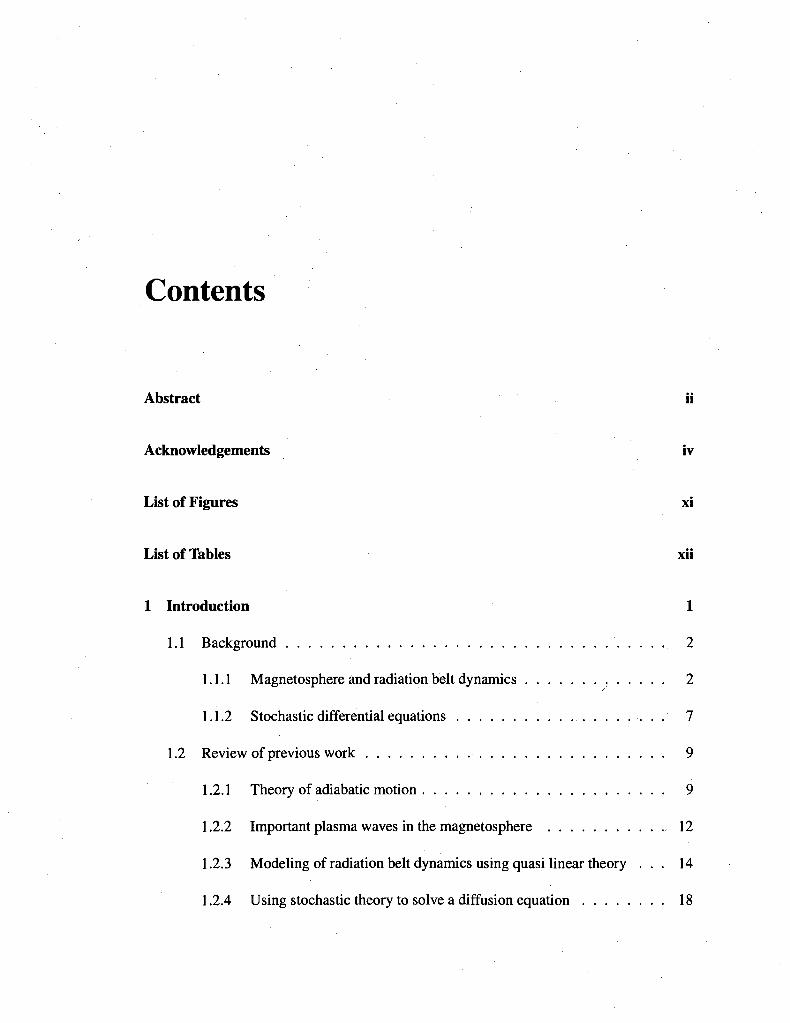
Contents

Abstract ii

Acknowledgements iv

List of Figures xi

List of Tables xii

1 Introduction 1

1.1 Background 2

1.1.1 Magnetosphere and radiation belt dynamics 2

1.1.2 Stochastic differential equations 7

1.2 Review of previous work 9

1.2.1 Theory of adiabatic motion 9

1.2.2 Important plasma waves in the magnetosphere 12

1.2.3 Modeling of radiation belt dynamics using quasi linear theory . . . 14

1.2.4 Using stochastic theory to solve a diffusion equation 18

vii

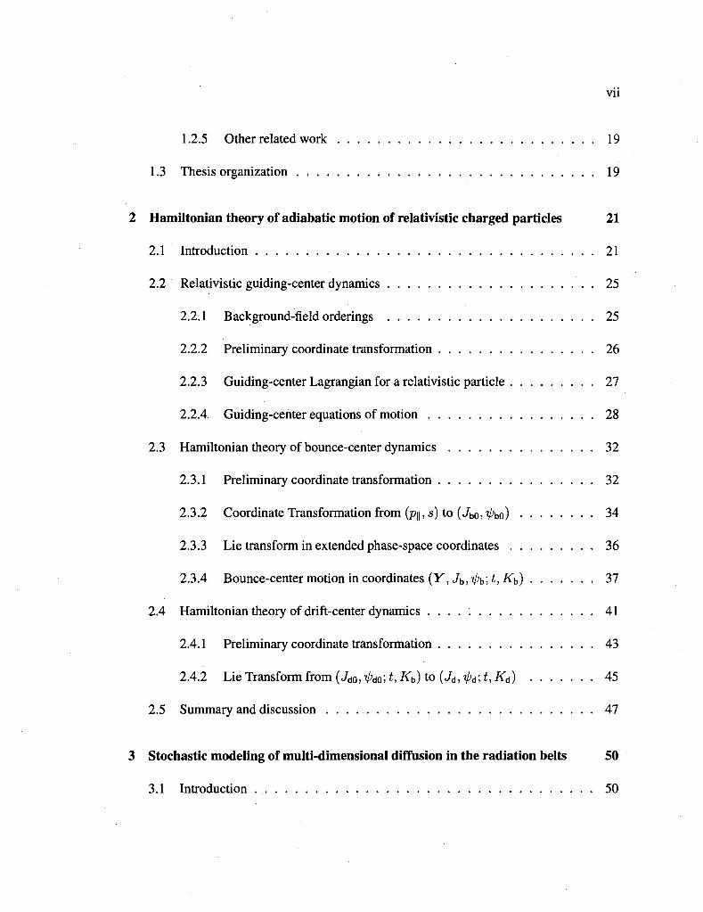
1.2.5 Other related work 19

1.3 Thesis organization 19

2 Hamiltonian theory of adiabatic motion of relativistic charged particles 21

2.1 Introduction 21

2.2 Relativistic guiding-center dynamics 25

2.2.1 Background-field orderings 25

2.2.2 Preliminary coordinate transformation 26

2.2.3 Guiding-center Lagrangian for a relativistic particle 27

2.2.4 Guiding-center equations of motion 28

2.3 Hamiltonian theory of bounce-center dynamics 32

2.3.1 Preliminary coordinate transformation 32

2.3.2 Coordinate Transformation from (p||, 5) to (JbO)V'bo) 34

2.3.3 Lie transform in extended phase-space coordinates 36

2.3.4 Bounce-center motion in coordinates {Y ,Jb,il)^\t,Kb) 37

2.4 Hamiltonian theory of drift-center dynamics 41

2.4.1 Preliminary coordinate transformation 43

2.4.2 Lie Transform from (JdOjV'do;*, Kb) to (Jd,ipd',t, Kd) 45

2.5 Summary and discussion 47

3 Stochastic modeling of multi-dimensional diffusion in the radiation belts 50

3.1 Introduction 50

viii

3.2 The SDE method 53

3.2.1 Ito stochastic differential equations . . . . 53

3.2.2 Probabilistic representation of solutions of diffusion equations . . . 54

3.3 Application 57

3.3.1 Application to pitch-angle and energy diffusion equations 58

3.3.2 Comparisons with Albert and Young [2005] results 61

3.3.3 Effects of parallel propagation approximation 65

3.4 Summary and discussion . 71

4 Modeling of multi-dimensional diffusion in radiation belts using layer methods 75

4.1 Introduction . 75

4.2 The Milstein layer methods 77

4.2.1 One-step representation of solutions using the SDE method . . . . . 77

4.2.2 A simple layer method algorithm 78

4.3 Application 80

4.3.1 Comparison with Albert and Young [2005] results . . 82

4.3.2 Effects of ignoring cross diffusion in Li et al. [2007] chorus wave

model 83

4.3.3 Evolution of electron fluxes using a model of fast magnetosonic

waves and hiss 90

4.4 Summary . . . 92

ix

5 Summary and future work 96

5.1 Summary 96

5.2 Discussion and future work 98

A Time-forward SDE method 102

B One-step error of the layer method 105

C Relationship between finite difference methods and layer methods 107

List of Figures

1.1 Earth's magnetosphere 3

1.2 The Van Allen radiation belts 4

1.3 Three adiabatic motions 5

1.4 Change of electron fluxes during a storm . . 8

1.5 Sample trajectories of two stochastic differential equations (SDEs) 10

1.6 A MLT distribution of plasma waves in the magnetosphere 15

3.1 Diffusion coefficients (D) repeated from Albert and Young [2005] 62

3.2 Comparisons between the SDE method results and previous results 64

3.3 Effects of cross diffusion using the Home et al. [2005] chorus wave model . 66

3.4 D of the Home et al. [2005] wave model with parallel propagation 67

3.5 Comparisons between fluxes obtained from D\ and D,i 69

3.6 Comparisons between fluxes obtained from D\ and D 70

3.7 Comparisons between fluxes obtained from D" and D 72

4.1 Convergence of solutions of layer methods with Nao and Ny 84

xi

4.2 Comparisons between the layer method results and previous results 85

4.3 D of the Li et al. [2007] chorus wave model with oblique waves . . . . . . 87

4.4 Flux evolution using the Li et al. [2007] chorus wave model 88

4.5 Effects of cross diffusion using the Li et al. [2007] chorus wave model . . . 89

4.6 D of the combined magnetosonic wave and hiss (MH) wave model 92

4.7 Flux evolution using the MH wave model 93

4.8 Effects of cross diffusion using the MH wave model 95

A.l Local effects of ignoring off-diagonal terms . 104

List of Tables

3.1 Parameters of the Home et al. [2005] wave model 63

4.1 Parameters of the Home et al. [2005] and Li et al. [2007] wave models . . . 82

Chapter 1

Introduction

This dissertation describes theoretical research on adiabatic relativistic charged particle

motion and numerical modeling of relativistic electron dynamics in the Earth's radiation

belts. The overall purpose is to improve understanding of physical processes responsible

for changes of electron fluxes in the radiation belts. Specifically, the purpose of this thesis

is to strengthen the foundation of theory and to develop numerical codes to model changes

of electron fluxes due to interactions with plasma waves. The increase of energetic electron

fluxes are potentially hazardous to satellites and astronauts in space [see Baker etal.,l994],

and the precipitation of electrons into the atmosphere can cause changes of chemistry of

the atmosphere and ozone destruction [e.g. Thome, 1977].

The main part of the thesis is divided into three chapters. In Chapter 2, we show a

Hamiltonian theory of three relativistic adiabatic motions in slowly varying electromag­

netic fields. The theory of adiabatic motion is the foundation of understanding radiation

1

2

belt dynamics. In Chapter 3 we show the stochastic differential equation (SDE) method

and Chapter 4 the layer method of modeling radiation belt dynamics using multidimen­

sional diffusion theory. While each method has its own advantages and disadvantages, both

methods can be used to solve multi-dimensional diffusion equations with cross diffusion

terms. The cross diffusion terms complicate the numerical problem and were ignored by

most of the previous work, thus in both chapters we explored their importance in radiation

belt modeling using different plasma wave models.

1.1 Background

In this section, we will first briefly describe the dynamics of Earth's magnetosphere and

radiation belts. Then we will introduce stochastic differential equations, which are basis of

the two numerical codes that we will develop later in the thesis.

1.1.1 Magnetosphere and radiation belt dynamics

The Earth's magnetosphere is the region of space that is dominated by the Earth's magnetic

field, whose main component can be described as a dipole field [Kivelson and Russell,

1995]. Because of the interaction with the solar wind, which is a magnetized plasma that

flows supersonically from the Sun, the magnetosphere is compressed in the dayside and

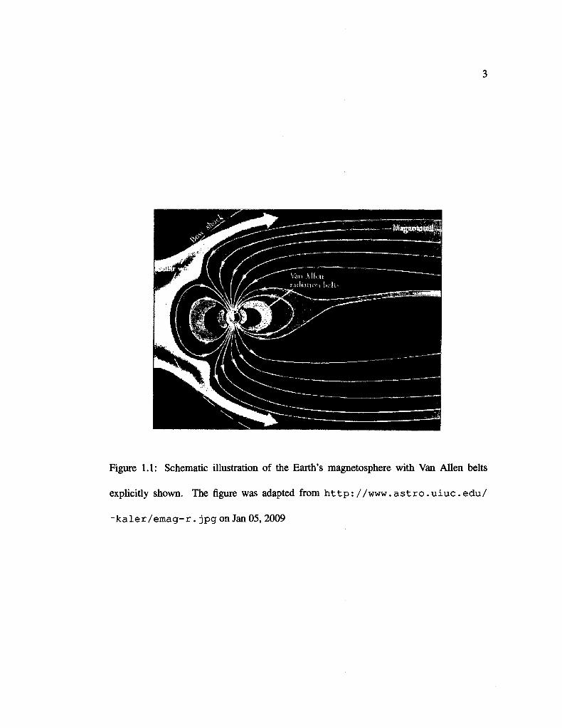
stretched in the tail side, as sketched in Figure 1.1. The magnetosphere can be very dy­

namic due to changes in solar wind conditions. A characteristic dynamic process is the

geomagnetic storm, which is a temporary large scale disturbance of the magnetosphere.

3

Figure 1.1: Schematic illustration of the Earth's magnetosphere with Van Allen belts

explicitly shown. The figure was adapted from h t t p : / / w w w . a s t r o . u i u c . e d u /

- k a l e r / e m a g - r . jpgonJan05, 2009

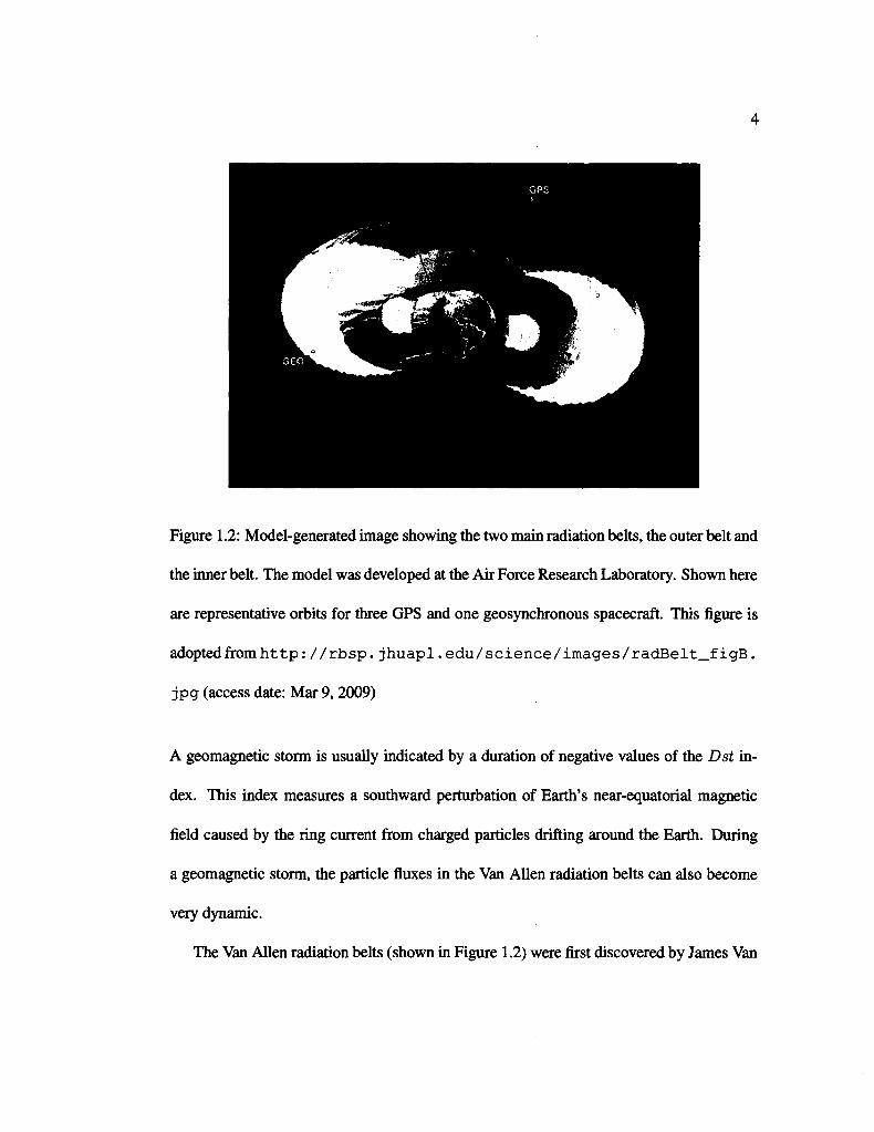
Figure 1.2: Model-generated image showing the two main radiation belts, the outer belt and

the inner belt. The model was developed at the Air Force Research Laboratory. Shown here

are representative orbits for three GPS and one geosynchronous spacecraft. This figure is

adopted from h t t p : / / r b s p . j h u a p l . e d u / s c i e n c e / i m a g e s / r a d B e l t _ f i g B .

jpg (access date: Mar 9,2009)

A geomagnetic storm is usually indicated by a duration of negative values of the Dst in­

dex. This index measures a southward perturbation of Earth's near-equatorial magnetic

field caused by the ring current from charged particles drifting around the Earth. During

a geomagnetic storm, the particle fluxes in the Van Allen radiation belts can also become

very dynamic.

The Van Allen radiation belts (shown in Figure 1.2) were first discovered by James Van

5

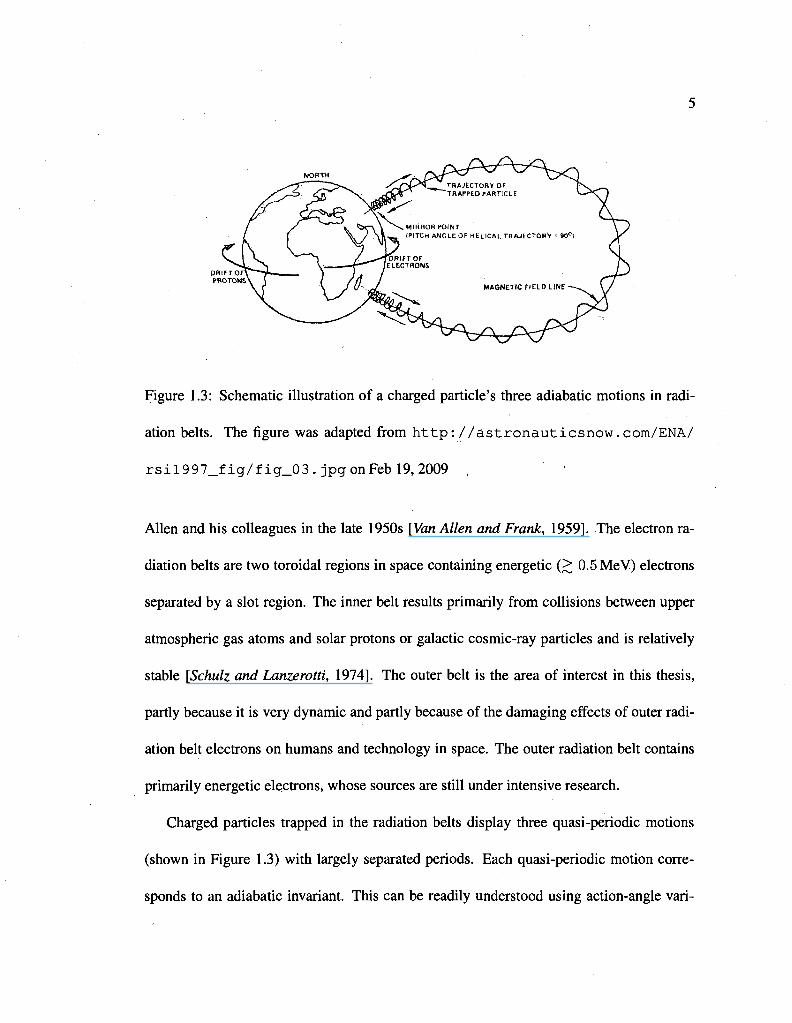
Figure 1.3: Schematic illustration of a charged particle's three adiabatic motions in radi­

ation belts. The figure was adapted from h t t p : / / a s t ronau t i c snow.com/ENA/

r s i l 9 9 7 _ f i g / f ig_03 . jpg on Feb 19, 2009

Allen and his colleagues in the late 1950s [Van Allen and Frank, 1959]. The electron ra­

diation belts are two toroidal regions in space containing energetic (> 0.5 MeV) electrons

separated by a slot region. The inner belt results primarily from collisions between upper

atmospheric gas atoms and solar protons or galactic cosmic-ray particles and is relatively

stable [Schulz and Lanzerotti, 1974]. The outer belt is the area of interest in this thesis,

partly because it is very dynamic and partly because of the damaging effects of outer radi­

ation belt electrons on humans and technology in space. The outer radiation belt contains

primarily energetic electrons, whose sources are still under intensive research.

Charged particles trapped in the radiation belts display three quasi-periodic motions

(shown in Figure 1.3) with largely separated periods. Each quasi-periodic motion corre­

sponds to an adiabatic invariant. This can be readily understood using action-angle vari-

6

ables in Hamiltonian dynamics [Schulz and Lanzerotti, 1974]. The fastest motion is a

gyromotion around a single magnetic field line, and the corresponding adiabatic invariant

is defined as // = p±2/2mB. Here p± is the momentum perpendicular to the local magnetic

field B, and m is the particle mass. The second adiabatic motion is the north-south bounce

motion between two mirror points, where the particle changes its direction of motion along

the field line. The second adiabatic invariant is J = §p\\ds, where p\\ is the momentum

parallel to B and the integral is along the bounce trajectory. The third adiabatic invariant is

due to the drift motion around the Earth, and is represented by the magnetic flux enclosed

by a particle's drift path $ = j>s B • dS. Another useful quantity related to the drift motion

is the Roederer L-shell: L = —27rk0/<bRE, where k0 is the magnetic dipole moment and

RE the radius of the Earth [Roederer, 1970]. Thus if $ is an adiabatic invariant, so is L. In

a dipole magnetic field, L = r/Rs, where r is a particle's radial distance to the center of

the Earth.

Electromagnetic fields that vary on a time scale comparable to one of the three periods

can violate the corresponding adiabatic invariant. A possible result of this is stochastic

changes of adiabatic invariants and thus the diffusion of electrons in phase space. It is

customary to discuss diffusion using pitch angle, which is the angle between the particle's

momentum and magnetic field, its energy, and L. Stochastic changes of particle's pitch

angle could cause losses of particles into the atmosphere, thus pitch angle diffusion is

generally considered as a loss mechanism [Schulz and Lanzerotti, 1974]. Because phase

space density usually has a negative gradient in energy, energy diffusion, on the other

7

hand, is considered as an important acceleration mechanism. Violating the third adiabatic

invariant causes changes of a particle's L. If the first and second invariants are conserved,

the particle's energy increases if it moves inward to the Earth [see Schulz and Lanzerotti,

1974, Chapter III.l].

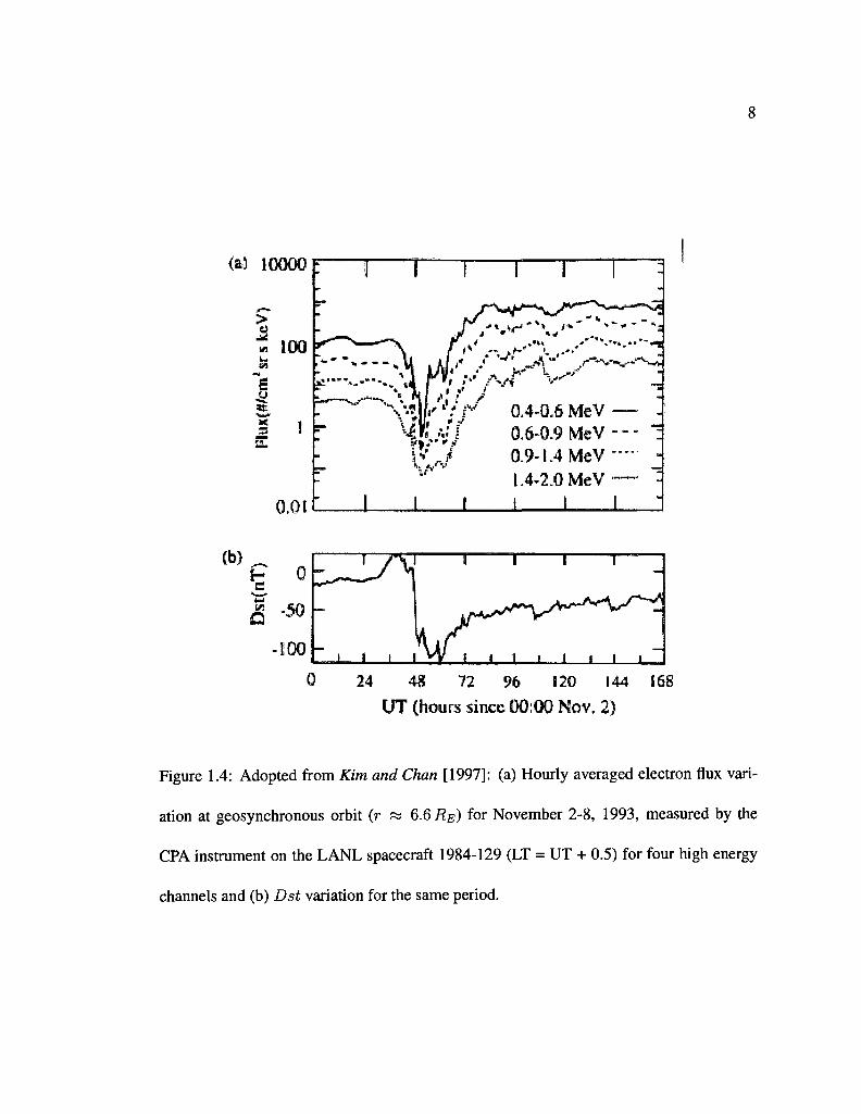
The quiet time radiation belt structure, including the slot region between the two belts,

has been explained by Lyons and Thome [1973] as an equilibrium between loss by pitch

angle scattering and inward radial diffusion. Changes of electron fluxes during a magnetic

storm are shown in the upper panel of Figure 1.4. We see that radiation belt electron fluxes

varied by several orders of magnitude during this storm. However, physical mechanisms for

acceleration and loss of energetic electrons are not well understood and are under research.

Reeves et al. [2003] analyzed 276 magnetic storms from 1989 through 2000, and concluded

that the dynamics of radiation belts are a complicated balance between electron loss and

acceleration. Possible mechanisms for loss and acceleration of electrons in the radiation

belts have been reviewed in Li and Temerin [2001]; Friedel et al. [2002]; Shprits et al.

[2008a] and Shprits et al. [2008b].

1.1.2 Stochastic differential equations

A stochastic differential equation (SDE) is used to describe a stochastic process, which is

utilized in this thesis to solve diffusion equations. In contrast to ordinary differential equa­

tions (ODEs), which are used to describe deterministic processes, SDEs contain stochastic

8

<*> IOOOO

>

42

-

0.0!

24 4g 72 96 120 144 168

UT (hours since 00:00 Nov, 2)

Figure 1.4: Adopted from Kim and Chan [1997]: (a) Hourly averaged electron flux vari­

ation at geosynchronous orbit (r « 6.6 RE) for November 2-8, 1993, measured by the

CPA instrument on the LANL spacecraft 1984-129 (LT = UT + 0.5) for four high energy

channels and (b) Dst variation for the same period.

9

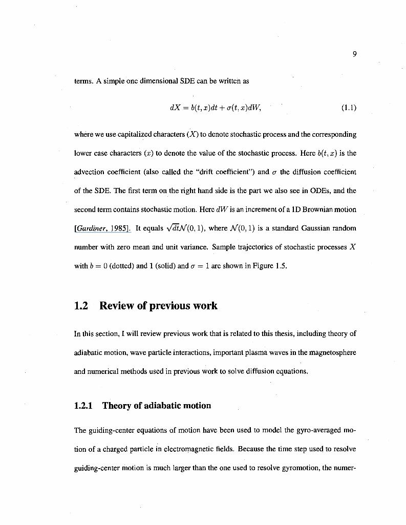
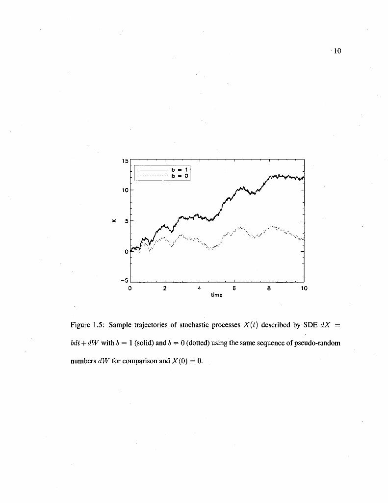
terms. A simple one dimensional SDE can be written as

dX = b{t,x)dt + a(t,x)dW, (1.1)

where we use capitalized characters (X) to denote stochastic process and the corresponding

lower case characters (x) to denote the value of the stochastic process. Here b(t, x) is the

advection coefficient (also called the "drift coefficient") and o the diffusion coefficient

of the SDE. The first term on the right hand side is the part we also see in ODEs, and the

second term contains stochastic motion. Here dW is an increment of a ID Brownian motion

[Gardiner, 1985]. It equals \/dij\f(0,1), where A/"(0,1) is a standard Gaussian random

number with zero mean and unit variance. Sample trajectories of stochastic processes X

with b = 0 (dotted) and 1 (solid) and a = 1 are shown in Figure 1.5.

1.2 Review of previous work

In this section, I will review previous work that is related to this thesis, including theory of

adiabatic motion, wave particle interactions, important plasma waves in the magnetosphere

and numerical methods used in previous work to solve diffusion equations.

1.2.1 Theory of adiabatic motion

The guiding-center equations of motion have been used to model the gyro-averaged mo­

tion of a charged particle in electromagnetic fields. Because the time step used to resolve

guiding-center motion is much larger than the one used to resolve gyromotion, the numer-

10

x 5h

Figure 1.5: Sample trajectories of stochastic processes X(t) described by SDE dX =

bdt + dW with b = 1 (solid) and 6 = 0 (dotted) using the same sequence of pseudo-random

numbers dW for comparison and X(0) = 0.

11

ical efficiency is increased usually by orders of magnitude. Northrop [1963] developed the

guiding-center equations of motion using a non-Hamiltonian method. A small parameter

e = p/l was used to order Northrop's guiding-center equations. Here p is the particle's gyro

radius, and I is the scale length of background magnetic fields. While this method is easy

to understand and straightforward, the resulting equations of motion do not conserve total

energy in static fields because higher order terms in e are ignored. Littlejohn [1981, 1983]

developed a new theory of guiding-center motion using a non-canonical Hamiltonian for­

mulation using Lie transform perturbation analysis [Cary and Littlejohn, 1983] for non-

relativistic particles. The resulting guiding-center equations conserve total energy in static

fields, and also conserve the extended Hamiltonian and phase-space volume in time-varying

fields. These conservation properties are useful for checking numerical accuracy. Another

advantage of the method is that the Lie transform analysis is systematic and can (in princi­

ple) be carried to arbitrary order. Brizard and Chan [2001] extended the work of Littlejohn

[1981] on guiding-center motion to relativistic particles in static fields. Further averaging

the guiding-center equation over the bounce-center phase angle will give us bounce-center

motion. Littlejohn [1982] derived the Hamiltonian theory of bounce-center motion (or

called by Littlejohn [1982] the guiding center bounce motion) for non-relativistic particles.

In this thesis, we will develop relativistic guiding-center and bounce-center Hamiltonian

theory and extend that to include the drift center motion in time-varying electromagnetic

fields.

12

1.2.2 Important plasma waves in the magnetosphere

Violations of adiabatic invariants can give rise to a variety of dynamical effects on the

radiation belts. Understanding the different processes responsible for electron acceleration

and loss is the main objective of radiation belt research.

One important process is radial diffusion, especially when enhanced by ULF (Ultra Low

Frequency, wave frequency / < 3 Hz) waves through drift resonance. The drift resonance

condition in a symmetric magnetic field is u — mu>d = 0, where u is the wave angular

frequency, u>d the particle drift frequency and m a positive integer. Radial diffusion has

been proposed as an acceleration mechanism of radiation belt electrons during storm times

[e.g., Schulz and Lanzerotti, 1974; Elkington et ah, 1999; Hilmer et ah, 2000]. However,

observations also show that during storm times, phase space densities of electrons can peak

around L ~ 5, and this cannot be explained by radial diffusion alone [Brautigam and

Albert, 2000; Green and Kivelson, 2004; Chen et al., 2007].

Resonant interactions with ELF (Extremely Low Frequency, 3 < / < 3000 Hz) and

VLF (Very Low Frequency, 3 < / < 30 kHz) waves have been invoked as an important

mechanism for electron local acceleration and precipitation via cyclotron resonances in

the radiation belts. Home and Thorne [1998] explored possible wave modes for electron

acceleration and loss via resonant wave-particle interactions using the resonance condition

LJ — k\\v\\ = nQ.e. (1.2)

Here LJ is the wave frequency, Qe is the electron relativistic gyrofrequency, and k\\ and

V|| are wave number and velocity parallel to B, respectively. Harmonic number n =

13

0, ±1, ±2, • • • with n = 0 the Landau resonance and n ^ 0 cyclotron resonance. By

calculating the minimum resonant energy needed for interacting with waves under storm-

time conditions, Home and Thome [1998] concluded that whistler mode waves and highly

oblique magnetosonic waves are possible candidates for accelerating electrons to the MeV

energy range, while electromagnetic ion cyclotron (EMIC) waves may only resonate with

highly relativistic electrons and contribute to loss via pitch-angle scattering. Other wave

modes possible for accelerating electrons include LO, RX and Z mode waves [see also,

Xiao et ah, 2006, 2007], but both more theoretical work and observations are needed to

determine their roles in radiation belt electron dynamics.

Plasmaspheric hiss waves and EMIC waves are under intensive research for their impor­

tant roles in loss of electrons in the radiation belts. Plasmaspheric hiss waves are whistler

mode, highly turbulent waves [Thome et ah, 1973]. These extremely low frequency (ELF)

hiss waves can cause electron loss into the atmosphere by pitch-angle scattering, which has

been included in several models [Abel and Thome, 1998a, b; Li et ah, 2007; Beutier and

Boscher, 1995; Bourdarie et ah, 1996; Meredith et ah, 2007]. EMIC waves can also reso­

nant with relativistic electrons and cause strong pitch-angle scattering [Albert, 2003; Sum­

mers and Thome, 2003; Li et ah, 2007; Albert, 2004; Khazanov and Gamayunov, 2007].

The main difference between hiss and EMIC waves shown by Li et ah [2007] is that EMIC

waves tend to cause electrons to diffuse into the loss cone while hiss waves tend to scatter

electrons from higher pitch angles to lower pitch angles but not necessarily into the loss

cone.

14

Chorus waves are whistler mode waves. Different from hiss and EMIC waves, they

have been associated with both loss and energization of radiation belt electrons through

pitch-angle diffusion and energy diffusion. Specifically, chorus waves have been related to

microburst precipitation of electrons [Lorentzen et ah, 2001; O'Brien et ah, 2003, 2004;

Thome et ah, 2005], but they are also possible candidates for energizing electrons during

storms [Home and Thome, 1998; Summers et ai, 1998; Meredith et ai, 2003a, b; Albert

and Young, 2005; Shprits et ai, 2006b]. A magnetic local time (MLT) distribution of the

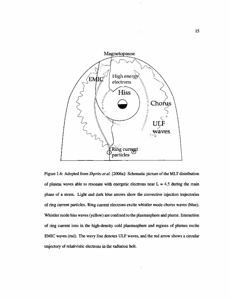
above plasma waves in the magnetosphere is shown schematically in Figure 1.6.

Recent observations show that fast magnetosonic waves (also known as equatorial

noise) might be related to electron acceleration in the radiation belts [Home et ah, 2007].

These waves propagate almost perpendicularly to background magnetic fields and thus in­

teract with electrons mainly through Landau resonance (n = 0) [Home et ah, 2007; Albert,

2008].

1.2.3 Modeling of radiation belt dynamics using quasi linear theory

Quasi linear diffusion theory is often used to model interactions between electrons and

waves. The term "quasi linear" is used because the time rate of change of the lowest order

distribution function is calculated nonlinearly from first order quantities, which are calcu­

lated using a linear theory. Kennel and Engelmann [1966] derived the quasi linear diffusion

equations for non-relativistic particles interacting via cyclotron resonances with small am­

plitude broad band oblique waves. Lyons [1974a] converted the diffusion coefficients of

15

Figure 1.6: Adopted from Shprits et al. [2006a]: Schematic picture of the MLT distribution

of plasma waves able to resonate with energetic electrons near L = 4.5 during the main

phase of a storm. Light and dark blue arrows show the convective injection trajectories

of ring current particles. Ring current electrons excite whistler mode chorus waves (blue).

Whistler mode hiss waves (yellow) are confined to the plasmasphere and plume. Interaction

of ring current ions in the high-density cold plasmasphere and regions of plumes excite

EMIC waves (red). The wavy line denotes ULF waves, and the red arrow shows a circular

trajectory of relativistic electrons in the radiation belt.

16

Kennel and Engelmann [1966] written in v\\ (velocity parallel to background magnetic field

B) and v± (velocity perpendicular to B) to pitch angle (a) and velocity (v) diffusion coef­

ficients. This work became the basis of later work of modeling of radiation belt dynamics

using quasi linear diffusion theory [Shprits et al, 2006b; Lam et al, 2007; Li et ah, 2007;

Home et al., 2007]. Typically, quasilinear diffusion in 3D is described by a Fokker-Planck

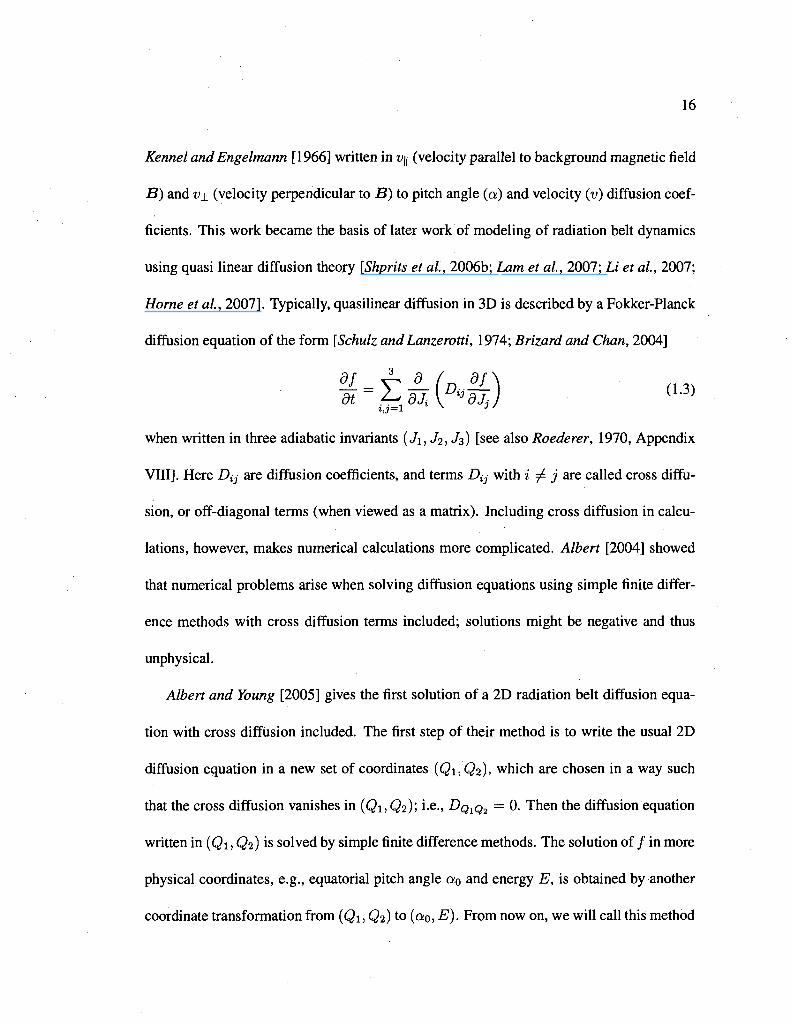
diffusion equation of the form [Schulz and Lanzewtti, 1974; Brizard and Chan, 2004]

1,3=1 J

when written in three adiabatic invariants (Ji, J2, J3) [see also Roederer, 1970, Appendix

VIII]. Here £>jj are diffusion coefficients, and terms Dij with i ^ j are called cross diffu­

sion, or off-diagonal terms (when viewed as a matrix). Including cross diffusion in calcu­

lations, however, makes numerical calculations more complicated. Albert [2004] showed

that numerical problems arise when solving diffusion equations using simple finite differ­

ence methods with cross diffusion terms included; solutions might be negative and thus

unphysical.

Albert and Young [2005] gives the first solution of a 2D radiation belt diffusion equa­

tion with cross diffusion included. The first step of their method is to write the usual 2D

diffusion equation in a new set of coordinates (Qi, Q%), which are chosen in a way such

that the cross diffusion vanishes in (Qi, Q2)\ i-e., DQ1Q2 = 0. Then the diffusion equation

written in (Qi, Q2) is solved by simple finite difference methods. The solution of / in more

physical coordinates, e.g., equatorial pitch angle ao and energy E, is obtained by another

coordinate transformation from (Q1( Q2) to (a0, E). From now on, we will call this method

17

the transformation method for simplicity.

Using the transformation method, Albert and Young [2005] solved a 2D diffusion equa­

tion using a ehorus wave model from Home et al. [2005] to show acceleration of electrons

by chorus waves. Their results show that chorus waves can accelerate electrons to MeV

energy on time scales of one day. To evaluate effects of cross diffusion, Albert and Young

[2005] then compared fluxes calculated with and without off-diagonal terms. They con­

cluded that for the Home et al. [2005] chorus wave model, ignoring cross diffusion does

not change flux profiles qualitatively, but quantitatively leads to an overestimate of energy

diffusion.

The transformation method is a nice method to solve 2D radiation belt diffusion equa­

tions; however, it does not generalize very well to 3D with all nine diffusion coefficients

in equation (1.3) included [personal communication, Jay M. Albert, 2007]. Also Albert

and Young [2005] only considers interactions between chorus waves and electrons, mainly

because only a chorus wave model was available at the time. More wave models [Li et al,

2007; Home et al, 2007] have been proposed since then, and they should be used to cal­

culate effects of cross diffusion with different wave models. Furthermore, we want to

verify the results of Albert and Young [2005] with an independent approach and a method

is needed to solve general 3D radiation belt diffusion equations. All the above reasons

motivate the second and third parts of this thesis; i.e., to solve multidimensional diffusion

equations using stochastic differential equations.

18

1.2.4 Using stochastic theory to solve a diffusion equation

A diffusion equation describes the evolution in time of a particle density function when the

underlying motion of the particle is stochastic. Accordingly, one can derive the Fokker-

Planck diffusion equation from stochastic differential equations that describe the particle

motion [Gardiner, 1985]. Also, from the Fokker-Planck equation we can obtain the corre­

sponding stochastic process, which can then be used to obtain a solution of the diffusion

equation.

There have been at least two methods to solve diffusion equations using SDEs. The first

method is to convert the diffusion equation to corresponding SDEs, which show stochastic

changes of phase space coordinates of particles. Using test particle simulations with these

SDEs, we can solve the corresponding diffusion equation [e.g., Alanko-Huotari et al, 2007;

Albright et al., 2003; Yamada et al, 1998]. Because this method describes particles mov­

ing forward in time, we will call this method the "time forward" SDE method. Secondly,

mathematical theory shows that the solution of a diffusion equation can be written as the

expectation value of a stochastic process evaluated under specific conditions [e.g., Freidlin,

1985; Costantini et al, 1998; Bossy et al, 2004; Zhang, 1999]. This method is a gener­

alized method of characteristics, which is used to solve advection equations. Because the

method samples trajectories of a stochastic process backward in time in the same sense as

the method of characteristics, we call this method the "time backward" SDE method. Since

we will use the "time backward" SDE method as the main numerical method in this thesis,

we will just use the term "SDE method" to refer to the "time backward" SDE method.

19

Based on the SDE method, Milstein [2002]; Milstein andTretyakov [2001] and Milstein

and Tretyakov [2002] developed layer methods, which are deterministic and more efficient

when solutions on a large number of grid points are needed. This is the third numerical

method that we will use in this thesis.

1.2.5 Other related work

The diffusion equation approach mentioned above is not the only method to model radi­

ation belt dynamics. Test particle simulation approaches, which solve the guiding-center

equations of motion or the full particle equation of motion, have also been widely used

[Elkington et al, 1999; Kress et al, 2007; Albert, 2002]. On the other hand, recent ob­

servations of large amplitude chorus waves [Cully et al, 2008; Cattell et al, 2008] have

raised questions about whether the quasi linear diffusion approach is suitable to describe

interactions between electrons and these large amplitude chorus waves. Nonlinear inter­

actions, like phase trapping, have been explored and applied to wave-particle interactions

in Earth's magnetosphere by several authors [e.g., Bell, 1984; Albert, 1993, 2000; Bortnik

et al, 2008]. However, in this thesis, we will assume that interactions between electrons

and chorus waves are described by the quasi linear diffusion theory.

1.3 Thesis organization

This remainder of this thesis is organized as follows. In Chapter 2, we show development

of a Hamiltonian theory of three adiabatic motions using the Lie-transform perturbation

20

method and the guiding-center equations of motion for a relativistic particle in slowly-

varying electromagnetic fields. The stochastic differential equation (SDE) method of solv­

ing multi-dimensional diffusion equations is described in Chapter 3, with a 2D stochastic

code developed to solve a bounce-averaged pitch-angle and energy diffusion equation. In

Chapter 4, we show the layer method, which is based on the SDE method but is determin­

istic, to solve multi-dimensional diffusion equations. Also, as an application of the layer

code, we show effects of including cross diffusion on evolution of electron fluxes using a

chorus wave model and a combined magnetosonic and hiss wave model. We summarize

our results and discuss possible future work in Chapter 5.

Chapter 2

Hamiltonian theory of adiabatic motion

of relativistic charged particles

This chapter has been published in Physics of Plasmas [Tao et ah, 2007].

2.1 Introduction

The concept of the adiabatic motion of a charged particle in magnetic fields is impor­

tant to research in space plasma physics and fusion physics [Northrop, 1963; Brizard

and Hahm, 2007]. Depending on the confining magnetic geometry, a particle may dis­

play three quasi-periodic or periodic motions. The fastest of these three motions is the

gyromotion about a magnetic field line (with frequency o>g). The second motion exists

when a particle bounces along a magnetic field line between two mirror points (with fre­

quency uib), because of nonuniformity along magnetic field lines. The slowest motion is

21

22

the drift motion across magnetic field lines (with frequency o;d) caused by perpendicu­

lar magnetic gradient-curvature drifts. In space physics (and especially in radiation-belt

physics [Schulz and Lanzerotti, 1974]), these frequencies are widely separated such that

UJS : Ub : u>d ~ e_1 : 1 : e, where e <C 1 is a small dimensionless ordering parameter to be

defined below. Associated with each periodic orbital motion, there exists a corresponding

adiabatic invariant. We use //, Jb and Jd for the three invariants constructed in this work;

to be consistent, we may also use Jg = (mc/q)fi, where m is the particle's rest mass and q

its charge.

The theory of the adiabatic motion of charged particles in electromagnetic fields has

been well developed by Northrop [1963]. However, the non-Hamiltonian method used

by Northrop resulted in dynamical equations that do not possess important conservation

properties like energy conservation in static fields, because of the absence of higher-order

terms from Northrop's equations. In later work, Littlejohn [1983] used a noncanoni-

cal phase-space transformation method, based on Lie-transform perturbation analysis, to

obtain the Hamiltonian formulation of guiding-center dynamics for nonrelativistic parti­

cles. By asymptotically removing the dependence on the gyrophase, the first invariant

Jg = (mc/q) /j, is obtained from the guiding-center Lagrangian by Noether's theorem.

The resulting Hamiltonian guiding-center equations of motion conserve total energy for

motion in static fields. In the present work, we use the Lie-transform perturbation anal­

ysis to develop a systematic Hamiltonian theory for relativistic guiding-center motion in

weakly time-dependent electromagnetic fields. Our relativistic guiding-center equations of

23

motion are expressed in semi-covariant form [Boghosian, 1987], which simplifies the previ­

ous work by Grebogi and Littlejohn [1984] (who extended their relativistic guiding-center

equations to include ponderomotive effects associated with the presence of high-frequency

electromagnetic waves) and generalizes earlier work by Brizard and Chan [1999] (who

considered guiding-center motion of a relativistic particle in static magnetic fields).

Phase-space Lagrangians are used in our perturbation analysis. Compared with the

usual configuration space Lagrangian of N independent variables, the corresponding phase

space Lagrangian contains 2N independent variables. Physical equations of motion can

be obtained by applying the variational principle to a phase space Lagrangian. The use of

phase-space Lagrangians is important to the Lie perturbation analysis due to their linearity

in the time derivatives [Littlejohn, 1983].

The derivation of relativistic guiding-center dynamics begins with the removal of the

gyrophase dependence from the particle phase-space Lagrangian. Since the condition for

these periodic motions to exist is that the time variations of the forces a particle experiences

should be slow compared to the particle's motion, we assume first that the electromagnetic

fields vary on the drift timescale. Thus we shall construct the first and second adiabatic

invariants from the particle's motion. While this ordering is not the most general case, it is

the most common one in practice [Littlejohn, 1983]. This procedure gives us the reduced

six-dimensional guiding-center Lagrangian and the first invariant Jg. Based on the guiding-

center Lagrangian, we further remove the bounce phase and obtain the bounce-averaged

guiding-center (or bounce-center) motion. The bounce-center Lagrangian for nonrelativis-

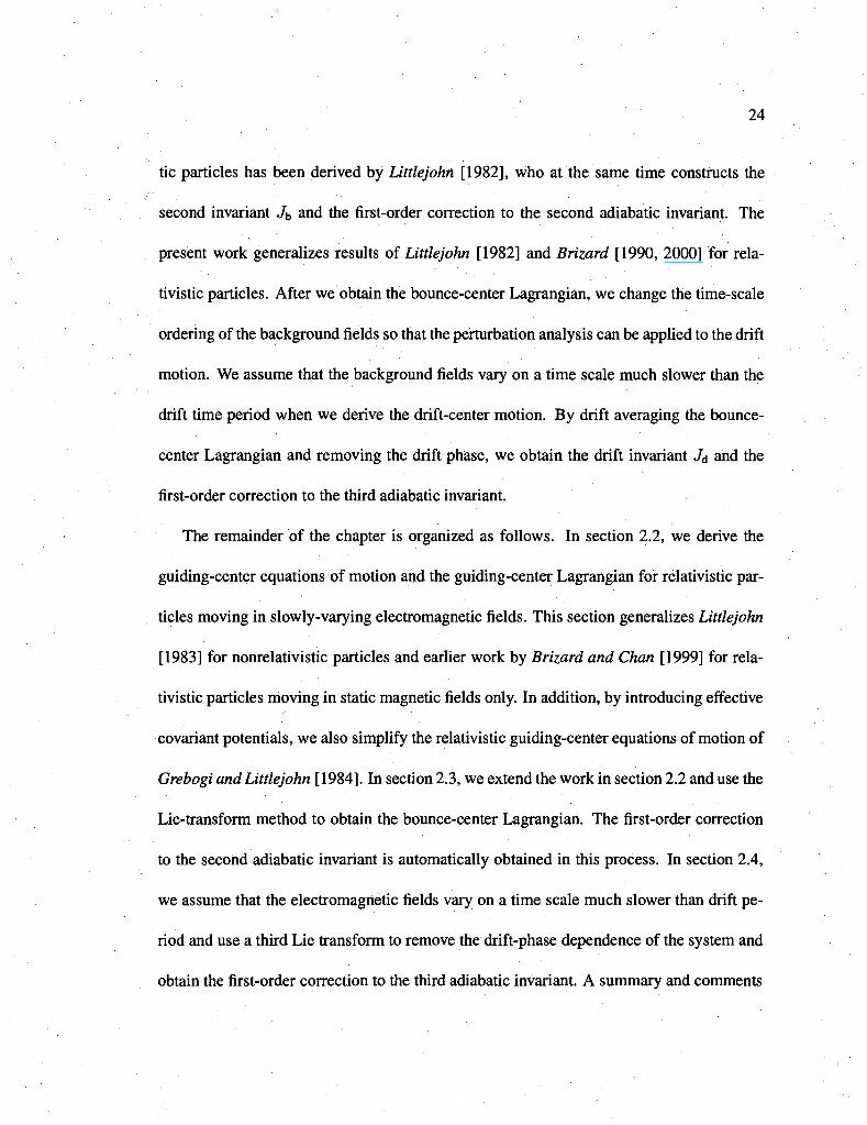
24

tic particles has been derived by Littlejohn [1982], who at the same time constructs the

second invariant J^ and the first-order correction to the second adiabatic invariant. The

present work generalizes results of Littlejohn [1982] and Brizard [1990, 2000] for rela-

tivistic particles. After we obtain the bounce-center Lagrangian, we change the time-scale

ordering of the background fields so that the perturbation analysis can be applied to the drift

motion. We assume that the background fields vary on a time scale much slower than the

drift time period when we derive the drift-center motion. By drift averaging the bounce-

center Lagrangian and removing the drift phase, we obtain the drift invariant J<j and the

first-order correction to the third adiabatic invariant.

The remainder of the chapter is organized as follows. In section 2.2, we derive the

guiding-center equations of motion and the guiding-center Lagrangian for relativistic par­

ticles moving in slowly-varying electromagnetic fields. This section generalizes Littlejohn

[1983] for nonrelativistic particles and earlier work by Brizard and Chan [1999] for rela­

tivistic particles moving in static magnetic fields only. In addition, by introducing effective

covariant potentials, we also simplify the relativistic guiding-center equations of motion of

Grebogi and Littlejohn [1984]. In section 2.3, we extend the work in section 2.2 and use the

Lie-transform method to obtain the bounce-center Lagrangian. The first-order correction

to the second adiabatic invariant is automatically obtained in this process. In section 2.4,

we assume that the electromagnetic fields vary on a time scale much slower than drift pe­

riod and use a third Lie transform to remove the drift-phase dependence of the system and

obtain the first-order correction to the third adiabatic invariant. A summary and comments

25

on further work are given in section 2.5.

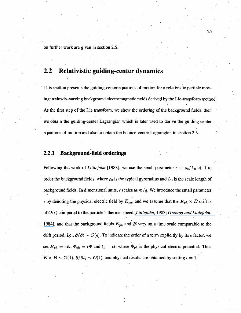
2.2 Relativistic guiding-center dynamics

This section presents the guiding-center equations of motion for a relativistic particle mov­

ing in slowly-varying background electromagnetic fields derived by the Lie-transform method.

As the first step of the Lie transform, we show the ordering of the background fields, then

we obtain the guiding-center Lagrangian which is later used to derive the guiding-center

equations of motion and also to obtain the bounce-center Lagrangian in section 2.3.

2.2.1 Background-field orderings

Following the work of Littlejohn [1983], we use the small parameter e = po/L0 «C 1 to

order the background fields, where p0 is the typical gyroradius and L0 is the scale length of

background fields. In dimensional units, e scales as m/q. We introduce the small parameter

e by denoting the physical electric field by Eph, and we assume that the Eph x B drift is

of 0(e) compared to the particle's thermal speed [Littlejohn, 1983; Grebogi and Littlejohn,

1984], and that the background fields Eph and B vary on a time scale comparable to the

drift period; i.e., d/dt ~ 0(e). To indicate the order of a term explicitly by its e factor, we

set Eph = eE, $p/i = e$ and t\ — et, where $p/, is the physical electric potential. Thus

E x B ~ 0(1), d/dti ~ 0(1), and physical results are obtained by setting e = 1.

26

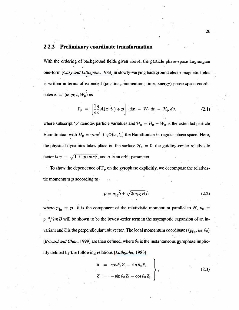
2.2.2 Preliminary coordinate transformation

With the ordering of background fields given above, the particle phase-space Lagrangian

one-form [Cary and Littlejohn, 1983] in slowly-varying background electromagnetic fields

is written in terms of extended (position, momentum; time, energy) phase-space coordi­

nates z = (x,p; t, Wp) as

TP 1 Q A , X --A(x,h) + p e c

dx - Wpdt - Hpda, (2.1)

where subscript 'p' denotes particle variables and Hp = Hp — Wp is the extended particle

Hamiltonian, with Hp = ^TTK? + q$>{x,t\) the Hamiltonian in regular phase space. Here,

the physical dynamics takes place on the surface Hp = 0, the guiding-center relativistic

factor is 7 = >/l + \p/mc\2, and a is an orbit parameter.

To show the dependence of Tp on the gyrophase explicitly, we decompose the relativis­

tic momentum p according to

p = phb+y/2mn0Bc, (2.2)

where p||0 = p • b is the component of the relativistic momentum parallel to B, /x0 =.

Px2/2mB will be shown to be the lowest-order term in the asymptotic expansion of an in­

variant and c is the perpendicular unit vector. The local momentum coordinates (p||0, /io, #o)

[Brizard and Chan, 1999] are then defined, where 6Q is the instantaneous gyrophase implic­

itly defined by the following relations [Littlejohn, 1983]

o = cos #o ei — sin 60 e~2 ) , (2.3)

c = — sin 80 e"i — cos 90 e~2

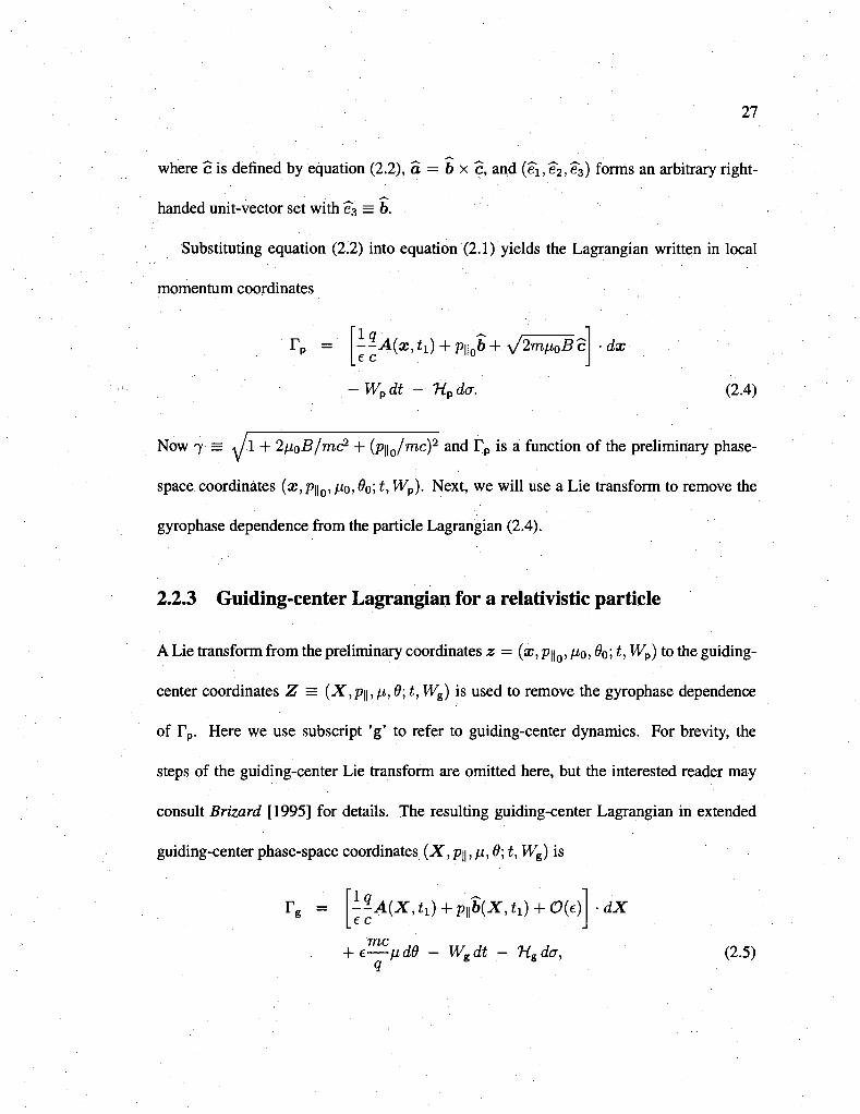
27

where c is defined by equation (2.2), a = b x c, and (ei,-e2, S3) forms an arbitrary right-

handed unit-vector set with e"3 = 6.

Substituting equation (2.2) into equation (2.1) yields the Lagrangian written in local

momentum coordinates

TP —A(x, ti) + pu.b +. \/2mnoB c • dx e c

-Wpdt — Hpda. (2.4)

Now 7 = J I + 2fi0B/mc2 + (p||0/mc)2 and r p is a function of the preliminary phase-

space coordinates (x,p\\Q, /i0, ^o! t, Wp). Next, we will use a Lie transform to remove the

gyrophase dependence from the particle Lagrangian (2.4).

2.2.3 Guiding-center Lagrangian for a relativistic particle

A Lie transform from the preliminary coordinates z — (x, p\\Q, fi0,90; t, Wp) to the guiding-

center coordinates Z = (X,p\\,ij,,9;t, Wg) is used to remove the gyrophase dependence

of Tp. Here we use subscript 'g' to refer to guiding-center dynamics. For brevity, the

steps of the guiding-center Lie transform are omitted here, but the interested reader may

consult Brizard [1995] for details. The resulting guiding-center Lagrangian in extended

guiding-center phase-space coordinates (X,p\\, fj,, 0; t, Wg) is

rg = l-^A{XM) + P\p{XM) + 0{e) dX

7TIC

+ e—/id6 - Wgdt - Heda, (2.5)

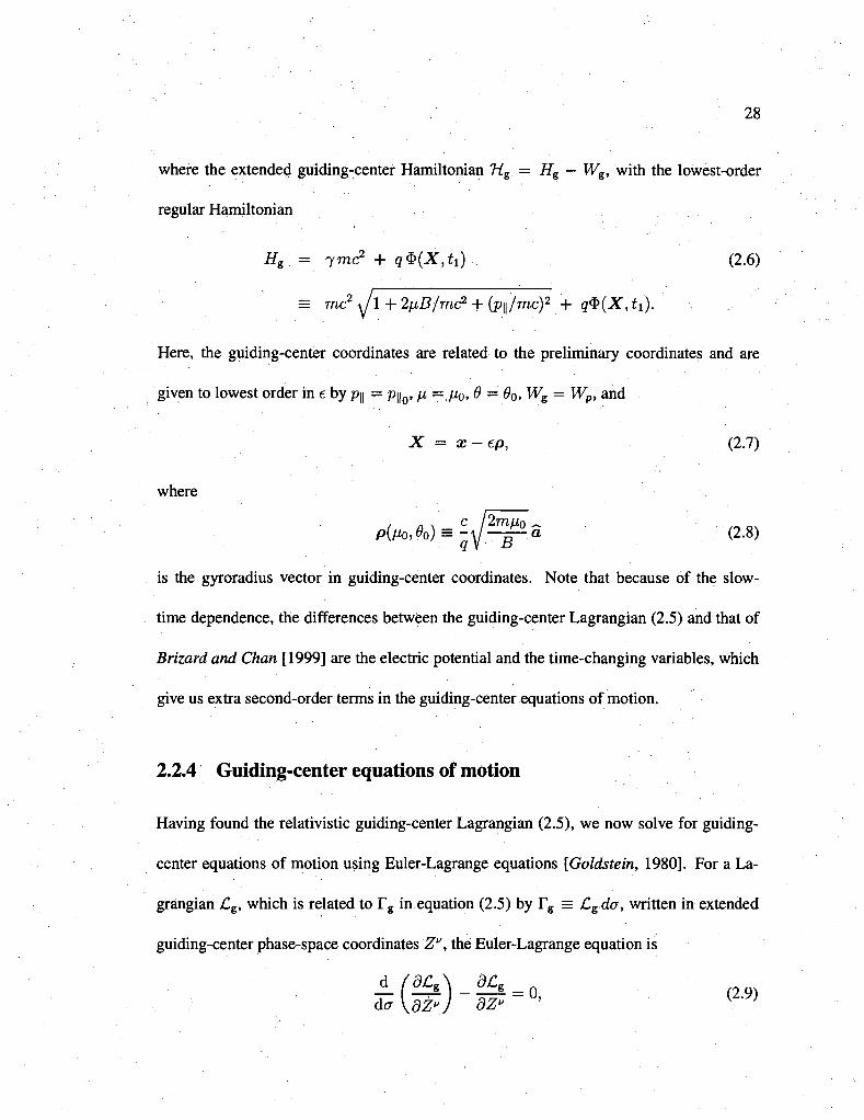
28

where the extended guiding-center Hamiltonian H.g = He — Ws, with the lowest-order

regular Hamiltonian

Hs = 7mc2.+ g$(X,ti)..-. (2.6)

= •• mc2 J\ + 2/j,B/mc2 + (p\\/mc)2 + q$(X,ti).

Here, the guiding-center coordinates are related to the preliminary coordinates and are

given to lowest order in e by p\\ = p\\Q, fi = ji0, 0 = 9o, Ws = Wp, and

X = x-ep, (2.7)

where

p{fl0,e0)^y2-^pa (2.8) is the gyroradius vector in guiding-center coordinates. Note that because of the slow-

time dependence, the differences between the guiding-center Lagrangian (2.5) and that of

Brizard and Chan [1999] are the electric potential and the time-changing variables, which

give us extra second-order terms in the guiding-center equations of motion.

2.2.4 Guiding-center equations of motion

Having found the relativistic guiding-center Lagrangian (2.5), we now solve for guiding-

center equations of motion using Euler-Lagrange equations [Goldstein, 1980]. For a La­

grangian £g, which is related to Tg in equation (2.5) by Tg = Cgda, written in extended

guiding-center phase-space coordinates Zu, the Euler-Lagrange equation is

-* ' = 0, (2.9) da \dZv dZv

29

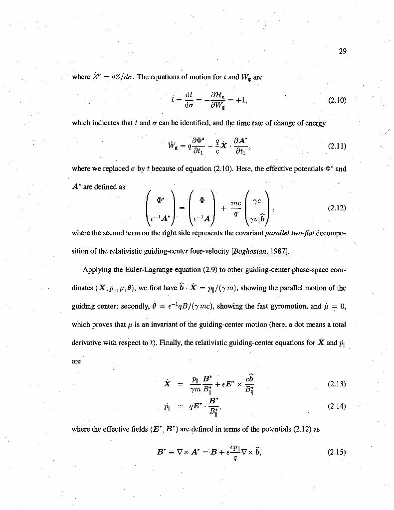
where Zv = dZ/da. The equations of motion for t and Wg are

'-§ dWe = +1, (2.10)

which indicates that t and cr can be identified, and the time rate of change of energy

Oti C Oti

where we replaced a by t because of equation (2.10). Here, the effective potentials $* and

A* are defined as

f v \

Y'IA"I V~1AI

I \ +

mc 7c

\nrvl{bj

(2.12)

where the second term on the right side represents the covariantpara//e/ two-flat decompo­

sition of the relativistic guiding-center four-velocity [Boghosian, 1987].

Applying the Euler-Lagrange equation (2.9) to other guiding-center phase-space coor­

dinates (X,p\\,/j,,0), we first have b • X = p\\/{"im), showing the parallel motion of the

guiding center; secondly, 0 = e~lqB/(^mc), showing the fast gyromotion, and (i = 0,

which proves that n is an invariant of the guiding-center motion (here, a dot means a total

derivative with respect to t). Finally, the relativistic guiding-center equations for X and p||

are

X =

P\\ =

irn B\ B\ ry*

qE'-—, q BV •

(2.13)

(2.14)

where the effective fields (E*,B*) are defined in terms of the potentials (2.12) as

.°Ph B* = Vx A* = B + e - ^ V x b, (2.15)

30

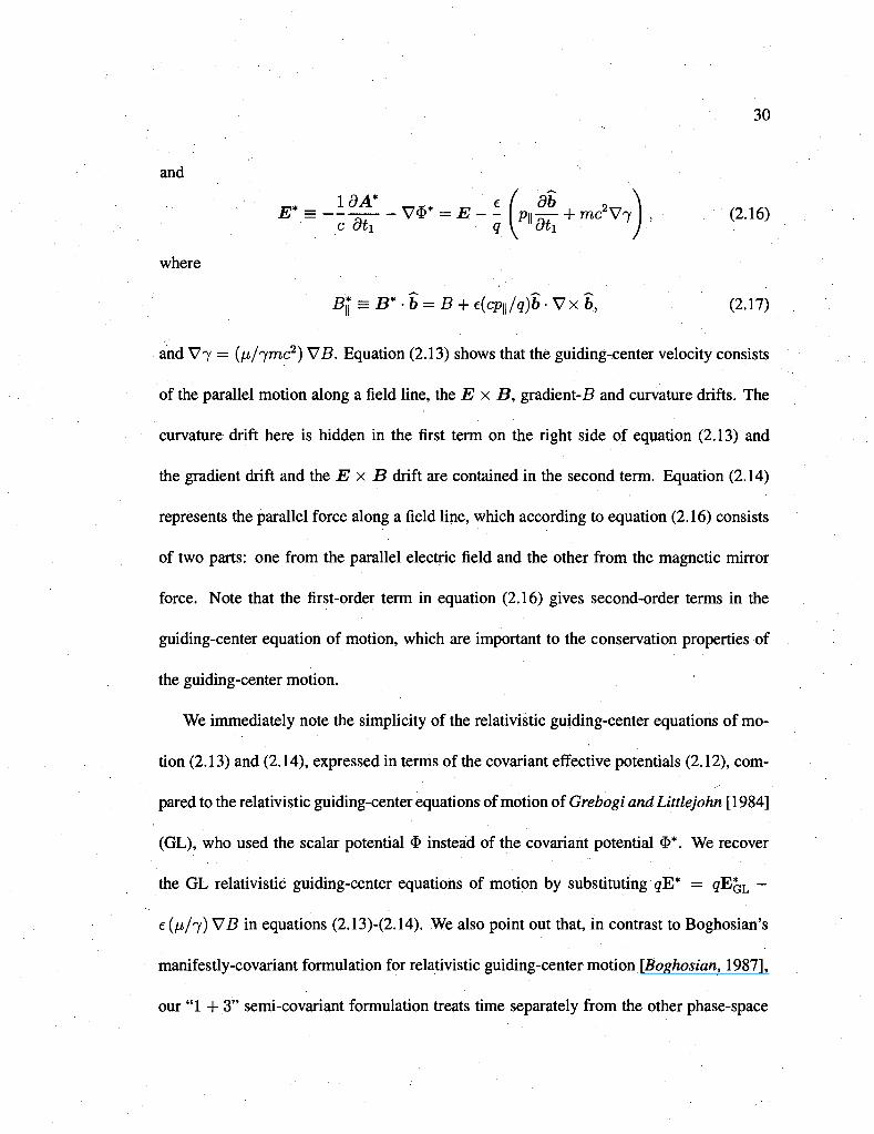
and

p s -T£ -v** -E - \ (*£+mc2V7) • (216)

where

Bl = B*-b = B + e(cPll/q)b-Vxb, (2.17)

and V7 = (fi/jmc2) VB. Equation (2.13) shows that the guiding-center velocity consists

of the parallel motion along a field line, the E x B, gradient-5 and curvature drifts. The

curvature drift here is hidden in the first term on the right side of equation (2.13) and

the gradient drift and the E x B drift are contained in the second term. Equation (2.14)

represents the parallel force along a field line, which according to equation (2.16) consists

of two parts: one from the parallel electric field and the other from the magnetic mirror

force. Note that the first-order term in equation (2.16) gives second-order terms in the

guiding-center equation of motion, which are important to the conservation properties of

the guiding-center motion.

We immediately note the simplicity of the relativistic guiding-center equations of mo­

tion (2.13) and (2.14), expressed in terms of the covariant effective potentials (2.12), com­

pared to the relativistic guiding-center equations of motion of Grebogi and Littlejohn [1984]

(GL), who used the scalar potential $ instead of the covariant potential $*. We recover

the GL relativistic guiding-center equations of motion by substituting qW = #EQL —

e (/VT) VB m equations (2.13)-(2.14). We also point out that, in contrast to Boghosian's

manifestly-covariant formulation for relativistic guiding-center motion [Boghosian, 1987],

our "1 + 3" semi-covariant formulation treats time separately from the other phase-space

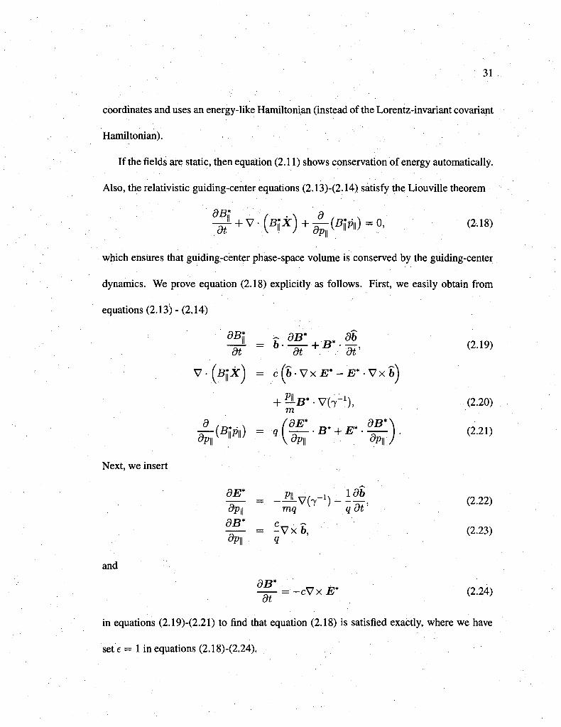
31

coordinates and uses an energy-like Hamiltonian (instead of the Lorentz-invariant covariant

Hamiltonian).

If the fields are static, then equation (2.11) shows conservation of energy automatically.

Also, the relativistic guiding-center equations (2.13)-(2.14) satisfy the Liouville theorem

BB* Ft

^r+v-(B"*) + ^ ( B W = 0' (2-18)

which ensures that guiding-center phase-space volume is conserved by the guiding-center

dynamics. We prove equation (2.18) explicitly as follows. First, we easily obtain from

equations (2.13)-(2.14)

dB* ^ dB* '3b

ST " b-Hf + Bm- (219)

V - ( s p f ) = c(b-VxE*-E*-Vxb^j

+ 21B* • V(7-1) , (2.20) m

Next, we insert

. .. ^ - - ^ V ( 7 - ) - i | , (2.22, op\\ mq q at

^ - = - V x S , (2.23) dp\\ q

and

BB* —— = -cVxE* (2.24)

at

in equations (2.19)-(2.21) to find that equation (2.18) is satisfied exactly, where we have

set e = 1 in equations (2.18)-(2.24).

32

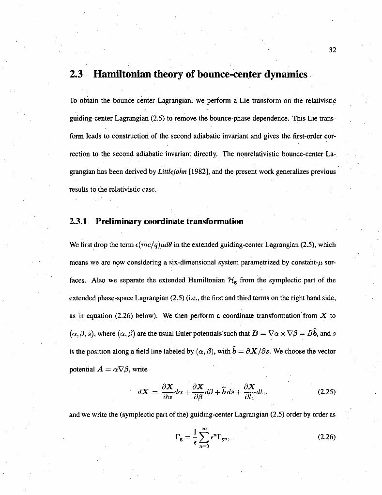
2.3 Hamiltonian theory of bounce-center dynamics

To obtain the bounce-center Lagrangian, we perform a Lie transform on the relativistic

guiding-center Lagrangian (2.5) to remove the bounce-phase dependence. This Lie trans­

form leads to construction of the second adiabatic invariant and gives the first-order cor­

rection to the second adiabatic invariant directly. The nonrelativistic bounce-center La­

grangian has been derived by Littlejohn [1982], and the present work generalizes previous

results to the relativistic case.

2.3.1 Preliminary coordinate transformation

We first drop the term e{mc/q)nd6 in the extended guiding-center Lagrangian (2.5), which

means we are now considering a six-dimensional system parametrized by constant-/^ sur­

faces. Also we separate the extended Hamiltonian 7ig from the symplectic part of the

extended phase-space Lagrangian (2.5) (i.e., the first and third terms on the right hand side,

as in equation (2.26) below). We then perform a coordinate transformation from X to

(a, f3, s), where (a, f3) are the usual Euler potentials such that B = Va x V/3 = Bb, and s

is the position along a field line labeled by (a, (3), with b = dX/ds. We choose the vector

potential A = a V/3, write

dX = —da + —df3 + bds + —dt1, (2.25) da d/3 ah

and we write the (symplectic part of the) guiding-center Lagrangian (2.5) order by order as

1 °° r g = - ^ 6 n r g n i (2.26)

n=0

33

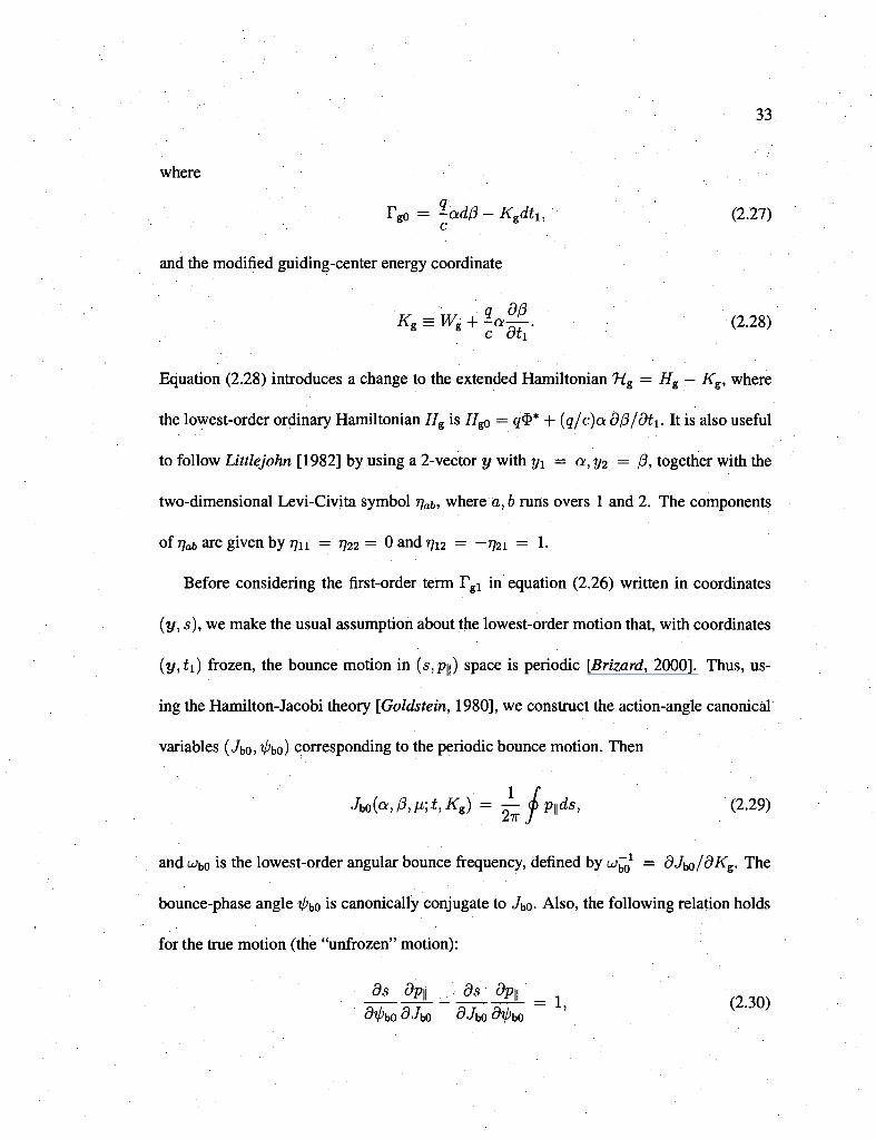
where

rg0 = -ad(3-Ksdti, (2.27)

and the modified guiding-center energy coordinate

Equation (2.28) introduces a change to the extended Hamiltonian Hg = Hg — Ks, where

the lowest-order ordinary Hamiltonian Hg is ifg0 = q$* + (q/c)a d/3/dti. It is also useful

to follow Littlejohn [1982] by using a 2-vector y with y1 = a,y2 = (3, together with the

two-dimensional Levi-Civita symbol 77 , where a, b runs overs 1 and 2. The components

of 7/a6 are given by ?7ii = 7722= 0 and r]12 = -r}2\ = 1.

Before considering the first-order term Tgl in equation (2.26) written in coordinates

(y, s), we make the usual assumption about the lowest-order motion that, with coordinates

(y,ti) frozen, the bounce motion in (s,P||) space is periodic [Brizard, 2000]. Thus, us­

ing the Hamilton-Jacobi theory [Goldstein, 1980], we construct the action-angle canonical

variables (Jbo, V'bo) corresponding to the periodic bounce motion. Then

JbQ(a,(3,n;t,Kg) = — (bp\\ds, (2.29)

and Wbo is the lowest-order angular bounce frequency, defined by w^1 = dJ^/dKg. The

bounce-phase angle >bo is canonically conjugate to Jbo- Also, the following relation holds

for the true motion (the "unfrozen" motion):

ds dp\\ ds dp\\

dipbo dJw dJw dipw = 1, (2.30)

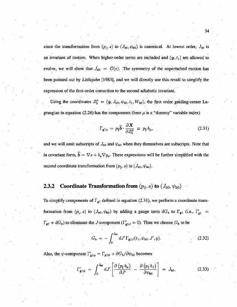
34

since the transformation from (p\\,s) to (Jbo,^bo) is canonical. At lowest order, Jb0 is

an invariant of motion. When higher-order terms are included and (y,ti) are allowed to

evolve, we will show that Jb0 = 0(e). The symmetry of the unperturbed motion has

been pointed out by Littlejohn [1983], and we will directly use this result to simplify the

expression of the first-order correction to the second adiabatic invariant.

Using the coordinates Z£ = (y, Jb0, V'bo, h, Wbo)> the first order guiding-center La-

grangian in equation (2.26) has the components (here // is a "dummy" variable index)

r g l p = p|tS • - ^ = -pn ^ , (2.31)

and we will omit subscripts of Jb0 and ^>b0 when they themselves are subscripts. Note that

in covariant form, b = Vs•+ baVya. These expressions will be further simplified with the

second coordinate transformation from (p\\,s) to (Jb0, V>bo)-

2.3.2 Coordinate Transformation from (p\\,s) to (Jbo, V'bo)

To simplify components of r g i defined in equation (2.31), we perform a coordinate trans­

formation from (p\\,s) to (Jt.cV'bo) by adding a gauge term dGb to Tgi (i.e., P g l =

Tgi + dGb) to eliminate the ./-component ( r g U = 0). Thus we choose Gb to be

fJbO

Gb=- dJTguOt^bo .Av)- (2.32) Jo

Also, the ^-component rgll/) = T^ + dGb/dipb0 becomes

d (pn fey,) d (pn 6j)

J O

JbO

dJ' dJ' dip{ bo

Jbo, (2.33)

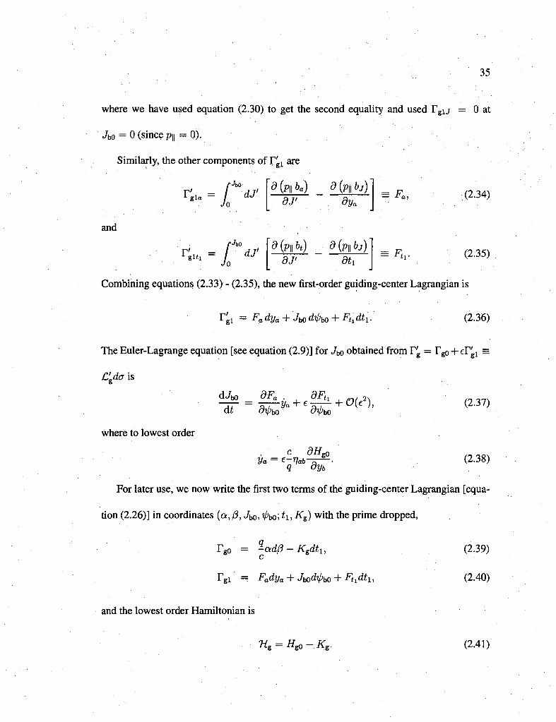
35

where we have used equation (2.30) to get the second equality and used TelJ = 0 at

Jb0 = 0(sincep|| =0) .

Similarly, the other components of T'gl are

^gla = / dJ' JO

and

r: gl i l / dJ' JO

d{p\\ba) dJ'

d (p|| bt)

dJ'

d(p\\ h) dya

d(pl{bj)

= Fa,

= Fty

(2.34)

(2.35)

Combining equations (2.33) - (2.35), the new first-order guiding-center Lagrangian is

Tgl = Fa dya '+ Jb0 dtpbo + Ftldti. (2.36)

The Euler-Lagrange equation [see equation (2.9)] for Jbo obtained from Tg = rg0 + eVgl =

C'da is 6

where to lowest order

dJi bO

dt &ip\

dFa . dFtl , 2.

bO di/>\ bO

c dHgn Va = e-Vab-^--

q oyb

(2.37)

(2.38)

For later use, we now write the first two terms of the guiding-center Lagrangian [equa­

tion (2.26)] in coordinates (a,/3, Jbo, V'bo! h, Kg) with the prime dropped,

1 Tgo = —ad/3 — Kgdti,

rg i = Fadya + Jbo#bO + Fhdti,

(2.39)

(2.40)

and the lowest order Hamiltonian is

^ g — ^go ~ Kg- (2.41)

36

With these coordinate transformations and Lagrangian, we do a Lie transform to remove

the bounce-phase dependence from Tg and obtain the bounce-center Lagrangian Tb.

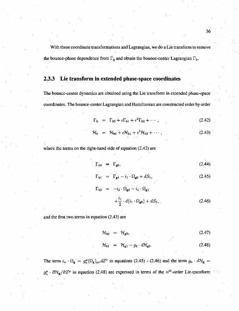
2.3.3 Lie transform in extended phase-space coordinates

The bounce-center dynamics are obtained using the Lie transform in extended phase-space

coordinates. The bounce-center Lagrangian and Hamiltonian are constructed order by order

r b = rb0 + e r b l + e2rb2 + • • •, (2.42)

Hb = Hb0 + eHbl + e2Hb2 + • • • , (2.43)

where the terms on the right-hand side of equation (2.42) are

rb0 = rg0, (2.44)

Tbi = ' r g i - * i - f i g 0 + dS1) (2.45)

r b 2 = — %2 • ^gO — H • " g l

+ Zj-d{i1-ngp) + dS2, (2.46)

and the first two terms in equation (2.43) are

'Wbo = Wgo, (2-47)

Hbi = Wgi-0i-dWgo. (2.48)

The term in • Qg = g^l^)iiVdZv in equations (2.45) - (2.46) and the term gn • dHe —

g£ • dHjdZ11 in equation (2.48) are expressed in terms of the nt/l-order Lie-transform

37

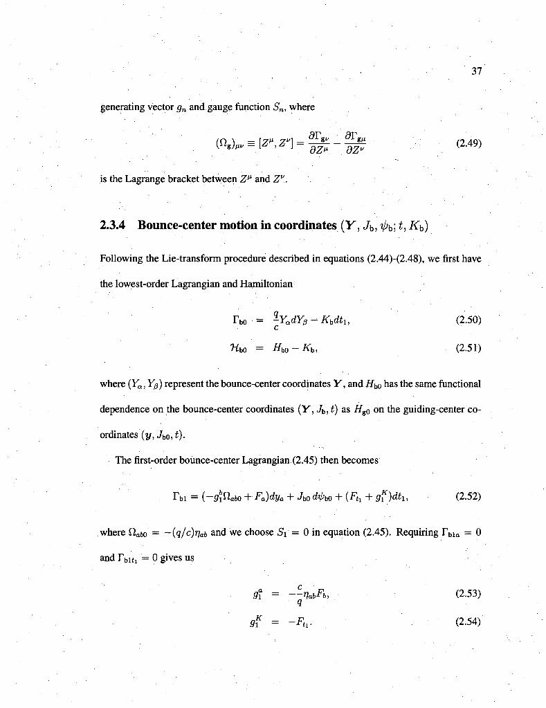
generating vector gn and gauge function Sn, where

( n . W ^ ^ Z l - ' ^ - ^ - . (2.49)

is the Lagrange bracket between Z^ and Zv.

2.3.4 Bounce-center motion in coordinates (Y,Jb,ipb;t,Kb)

Following the Lie-transform procedure described in equations (2.44)-(2.48), we first have

the lowest-order Lagrangian and Hamiltonian

rbo = -YadY,3 - Kbdtu (2.50)

Wbo = ^bo — Kb, (2.51)

where (Ya, Yp) represent the bounce-center coordinates Y, and ifbo has the same functional

dependence on the bounce-center coordinates (Y, Jb, t) as ifg0 on the guiding-center co­

ordinates (y,Jbo,t).

The first-order bounce-center Lagrangian (2.45) then becomes

Tbi = (-9b1Ctabo+Fa)dya + Jbodipbo + (Ftl+g^)dtu (2.52)

where f2ato = —(l/c)Vab and we choose Si = 0 in equation (2.45). Requiring r b i a = 0

and Tbitj = 0 gives us

Sli = --VabFb, (2.53)

9i = -Ft,- (2.54)

38

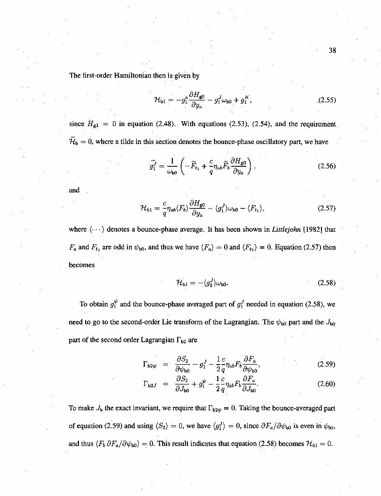
The first-order Hamiltonian then is given by

Hbl = -ga1-^-gJ

1ub0 + gK, (2.55)

since Hgi = 0 in equation (2.48). With equations (2.53), (2.54), and the requirement

Hb = 0, where a tilde in this section denotes the bounce-phase oscillatory part, we have

9{ = — (-Ftl + -VabFb^), (2.56) Wbo V q oya J

and

Hbl = -Vah(Fb)^-(gJ1)ujb0-(Ftl), (2.57)

where (• • •) denotes a bounce-phase average. It has been shown in Littlejohn [1982] that

Fa and Ftl are odd in ^bOvand thus we have (Fa) = 0 and (Ftl) = 0. Equation (2.57) then

becomes

Hbl = -{g{)uto. (2-58)

To obtain gf and the bounce-phase averaged part of g{ needed in equation (2.58), we

need to go to the second-order Lie transform of the Lagrangian. The V>bo part and the Jbo

part of the second order Lagrangian 1 2 are

r dS* J l c rdF" nia-x rb2V = Q-; 9i ~ n-VabFb^—, (2.59)

8S2 ^ Ic dFa

Tb2J = 5 7 - + gt - o-VabFbjr—. (2.60)

To make Jb the exact invariant, we require that Fb2^ = 0. Taking the bounce-averaged part

of equation (2.59) and using (S^) = 0, we have (g{) = 0, since dFa/dil)bQ is even in ^M,

and thus (Fb dFa/dtpw) = 0. This result indicates that equation (2.58) becomes Hb\ = 0.

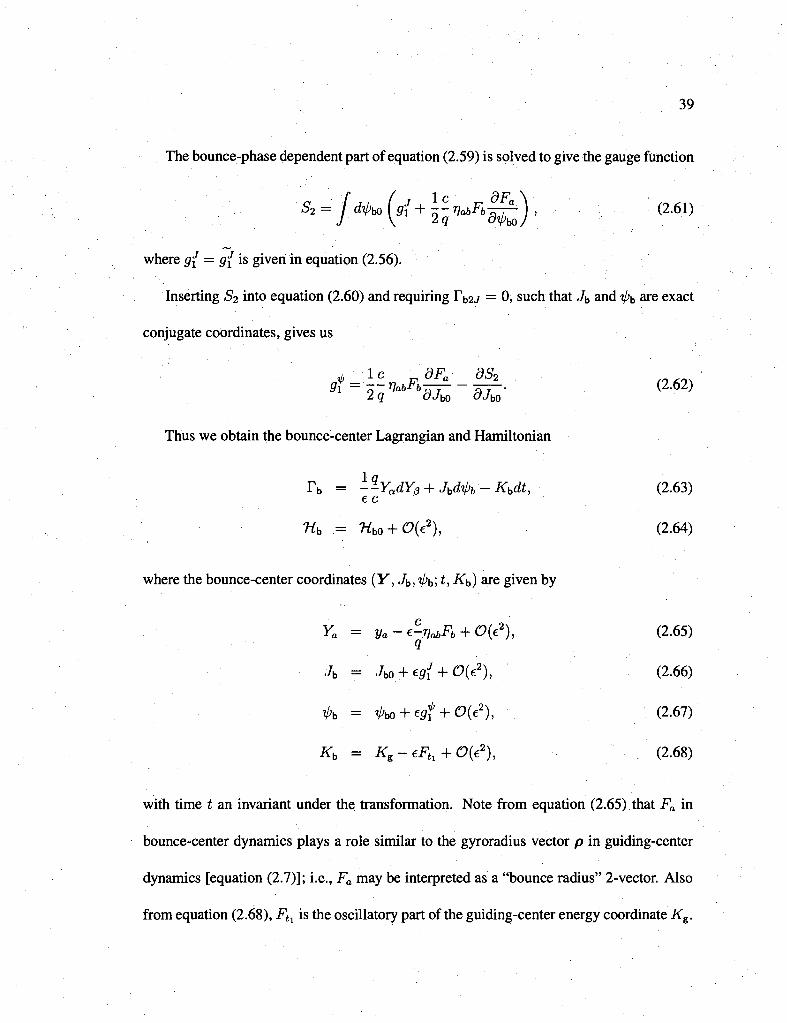
39

The bounce-phase dependent part of equation (2.59) is solved to give the gauge function

where g( = g{ is given in equation (2.56).

Inserting S2 into equation (2.60) and requiring Tb2j = 0, such that Jb and ipb are exact

conjugate coordinates, gives us

gt = rq^Fia^-a^- (2-62)

Thus we obtain the bounce-center Lagrangian and Hamiltonian

Tb = -t-YadYp + Jbd4>b-Kbdt, (2.63) e c

Hb = Hbo + Oie2), (2.64)

where the bounce-center coordinates (Y, Jb, V'b! *> ^t>) are given by

Ya = ya-e-VabFb + Oie2),. (2.65)

Jb = Jbo + c ^ + OCc2), (2.66)

A = rpw + egt + 0(e2), (2.67)

tfb = Ke-eFtl + 0{e2), (2.68)

with time £ an invariant under the transformation. Note from equation (2.65) that Fa in

bounce-center dynamics plays a role similar to the gyroradius vector p in guiding-center

dynamics [equation (2.7)]; i.e., Fa may be interpreted as a "bounce radius" 2-vector. Also

from equation (2.68), Ftl is the oscillatory part of the guiding-center energy coordinate K%.

Ya

tpb

X

K,

—

—

=

c e-Vab

Q

dJb '

o, &Hb

dYb'

40

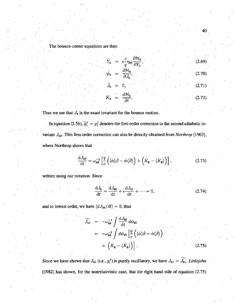
The bounce-center equations are then

AT-/.

(2.69)

(2.70)

(2.71)

. . . m . (2.72)

Thus we see that Jb is the exact invariant for the bounce motion.

In equation (2.56), gf = g( denotes the first-order correction to the second adiabatic in­

variant Jbo- This first-order correction can also be directly obtained from Northrop [1963],

where Northrop shows that

^ = otf-Ji ((a)/?- d</?>) + (*, - (Ke))] , (2.73)

written using our notation. Since

. t = ^ + - ^ and to lowest order, we have (dJbo/dt) = 0, thus

7- -if dJbo , , <4i = ~^bo / -^fdipbo

=-^y^bo^^-d^))

+ (tfg-<tf6))]. (2.75)

Since we have shown that Jbi (i.e., g{) is purely oscillatory, we have Jb\ = Jbi- Littlejohn

[1982] has shown, for the nonrelativistic case, that the right hand side of equation (2.75)

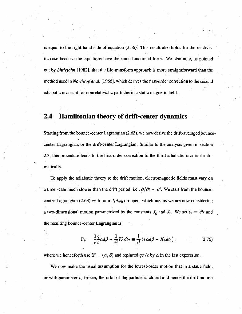
41

is equal to the right hand side of equation (2.56). This result also holds for the relativis-

tic case because the equations have the same functional form. We also note, as pointed

out by Littlejohn [1982], that the Lie-transform approach is more straightforward than the

method used in Northrop et al. [1966], which derives the first-order correction to the second

adiabatic invariant for nonrelativistic particles in a static magnetic field.

2.4 Hamiltonian theory of drift-center dynamics

Starting from the bounce-center Lagrangian (2.63), we now derive the drift-averaged bounce-

center Lagrangian, or the drift-center Lagrangian. Similar to the analysis given in section

2.3, this procedure leads to the first-order correction to the third adiabatic invariant auto­

matically.

To apply the adiabatic theory to the drift motion, electromagnetic fields must vary on

a time scale much slower than the drift period; i.e., d/dt ~ e2. We start from the bounce-

center Lagrangian (2.63) with term J^dip^ dropped, which means we are now considering

a two-dimensional motion parametrized by the constants Jg and Jb. We set t2 = e2t and

the resulting bounce-center Lagrangian is

Tb = -?-ad(3 - -^Kbdt2 = - (ead/3 - Kbdt2), (2.76)

where we henceforth use Y = (a, (3) and replaced qa/c by a in the last expression.

We now make the usual assumption for the lowest-order motion that in a static field,

or with parameter t2 frozen, the orbit of the particle is closed and hence the drift motion

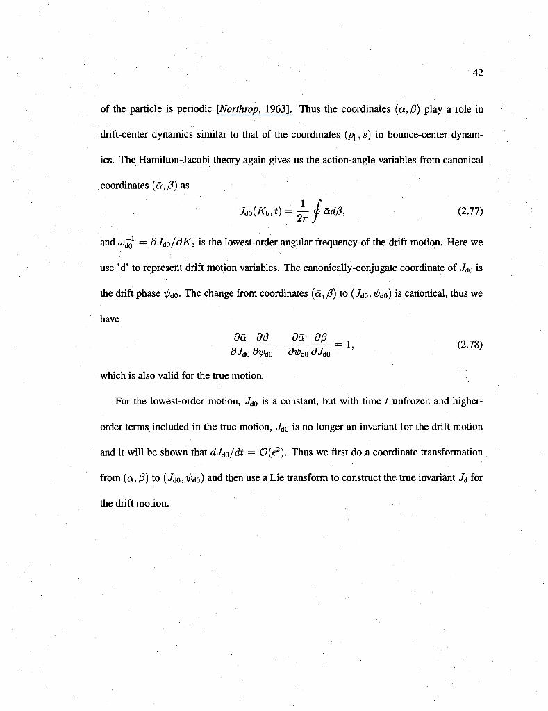
• 4 2

of the particle is periodic [Northrop, 1963]. Thus the coordinates (a,/3) play a role in

drift-center dynamics similar to that of the coordinates (p\\, s) in bounce-center dynam­

ics. The Hamilton-Jacobi theory again gives us the action-angle variables from canonical

coordinates (a, 0) as

MKb,t) = -^jadp, (2.77)

and UJ^Q = dJdo/dKb is the lowest-order angular frequency of the drift motion. Here we

use 'd' to represent drift motion variables. The canonically-conjugate coordinate of Jdo is

the drift phase tpdo- The change from coordinates (a, /?) to (Jd0, ipao) is canonical, thus we

have

da__dft__^oL^_ = 1' ( 2 7 g ) dJdodipao dipdodJdo

which is also valid for the true motion.

For the lowest-order motion, Jdo is a constant, but with time t unfrozen and higher-

order terms included in the true motion, Jdo is no longer an invariant for the drift motion

and it will be shown that dJd0/dt = 0(e2). Thus we first do a coordinate transformation

from (a, f3) to (Jd0, V'do) and then use a Lie transform to construct the true invariant Jd for

the drift motion.

' • ' 4 3

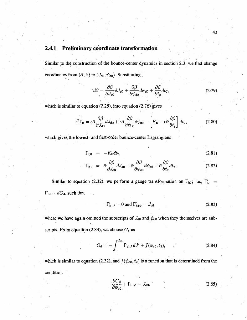
2.4.1 Preliminary coordinate transformation

Similar to the construction of the bounce-center dynamics in section 2.3, we first change

coordinates from (a,/?) to (JdcV'do)-Substituting

AR 9f3 AT UL QP A, ±WA*

dJdQ oipM. dt2

which is similar to equation (2.25), into equation (2.76) gives

2„ _ d/3 , T . • _ dp , , ezrb = ea-—rdJM + ea——#do -

' -d/3 Kb - ecu—

ot2

dt2,

which gives the lowest- and first-order bounce-center Lagrangians

(2.79)

(2.80)

Tbo = —Kbdt2,

_ dp , T .dp ,, _dp' Ibi = a-^—a^do + a-^— "V'do + a- —a<2-

dJd0 a-0do ot2

(2.81)

(2.82)

Similar to equation (2.32), we perform a gauge transformation on Tbl; i.e., r'bl =

Tbi + dGd, such that

r'bU = 0 and 1*,^ = Jd0, (2.83)

where we have again omitted the subscripts of Jdo and f/'do when they themselves are sub­

scripts. From equation (2.83), we choose Gd as

fJ<S0 /"JdO

Gd = - rblJdJ' + f(xl;d0,t2), Jo

(2.84)

which is similar to equation (2.32), and f(ipdo, h) is a function that is determined from the

condition

8Gd

'do + Tbi . = J( d0- (2.85)

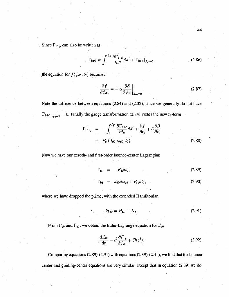
44

Since Pbi^ can also be written as

rJbo

biv> = / b 0 ^ ? ^ ' + r b i 4 , b o = o . (2.86)

the equation for /(V'ao, h) becomes

df _ d(3 = — a-

(2.87) 4,0=0 dipdo dipd0\

Note the difference between equations (2.84) and (2.32), since we generally do not have

Tbiv-I j =o = 0- Finally the gauge transformation (2.84) yields the new £2-term

* - - / blt2 - /

JO

Jd0 dTblJ df d(3 dJ + 7; r Oi—— dt<i dt2 dt2

= F t 2(Jd o ,Vdo,i2) . (2.88)

Now we have our zeroth- and first-order bounce-center Lagrangian

r b 0 = -Kbdt2, (2.89)

• Tbl =.JMdipM + Ft2dt2,: ,. (2.90)

where we have dropped the prime, with the extended Hamiltonian

nb0 = Hb0-Kb. (2.91)

From Tbo and rb i , we obtain the Euler-Lagrange equation for Jd0

^ = e 2 | ^ + 0(e3). (2.92) dt dipdo

Comparing equations (2.89)-(2.91) with equations (2.39)-(2.41), we find that the bounce-

center and guiding-center equations are very similar, except that in equation (2.89) we do

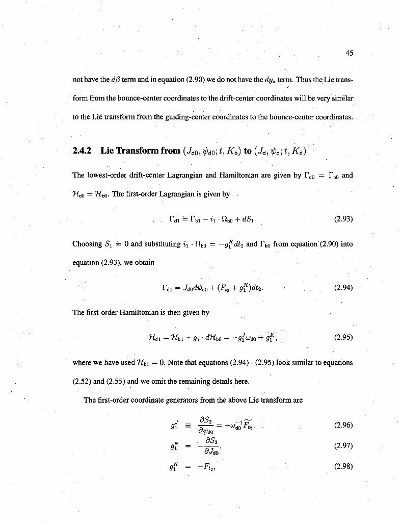
45

not have the df3 term and in equation (2.90) we do not have the dya term. Thus the Lie trans­

form from the bounce-center coordinates to the drift-center coordinates will be very similar

to the Lie transform from the guiding-center coordinates to the bounce-center coordinates.

2.4.2 Lie Transform from (Jd0, ipdo; t, Kb) to (Jj, ^ ; £, ifj) •

The lowest-order drift-center Lagrangian and Hamiltonian are given by rd0 = rb0 and

'Hdo = 7"4o- The first-order Lagrangian is given by

rdi = r b i - t i . -nbo + d5i. (2.93)

Choosing Si = 0 and substituting ij • f2b0 = —g^dt2 and r b l from equation (2.90) into

equation (2.93), we obtain

r d l = JMdi>M + (Ft2+g?)dt2. (2.94)

The first-order Hamiltonian is then given by

Wdi = Wbi " 9x • dHb0 = -g(u}M + g?, (2.95)

where we have used Hbi = 0. Note that equations (2.94) - (2.95) look similar to equations

(2.52) and (2.55) and we omit the remaining details here.

The first-order coordinate generators from the above Lie transform are

a o . 9( = ^£- = -^0

lFt2, (2.96)

rf = - # > (2.97). CJdo

9?- = ~Ft2, (2.98)

46

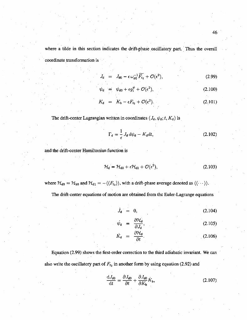
where a tilde in this section indicates the drift-phase oscillatory part. Thus the overall

coordinate transformation is

Jd = Jdo-euj^F\2 + 0{e2), (2.99)

V>d = ^o + egt + 0{e2), (2.100)

Kd = Kb-eFt2 + 0(e2). (2.101)

The drift-center Lagrangian written in coordinates (Jd, tpd; t, Kd) is

Td = -Jdd^d-Kddt, (2.102) • ' e

and the drift-center Hamiltonian function is

Hd = Hd0 + eHdl + O{e2), (2.103)

where Hdo = H^ and Hdi = —({Ft2)), with a drift-phase average denoted as ((• • •)).

The drift-center equations of motion are obtained from the Euler-Lagrange equations

. . • . j d " = 0, (2.104)

d = ? T ' (2-105> OJd

Kd = *£. (2.106)

Equation (2.99) shows the first-order correction to the third adiabatic invariant. We can

also write the oscillatory part of Ft2 in another form by using equation (2.92) and

dJd0 dJdQ dJd0 y

~TT ~*T + ~^TFK^ (2.107) dt at oKb

47

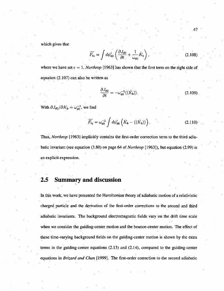
which gives that

=•*-/«% $r+£*>). <2>°« where we have set e = 1. Northrop [1963] has shown that the first term on the right side of

equation (2.107) can also be written as

dJdo _ _i dt

= -uj^{(Kb)). (2.109)

With dJdo/dKb = udQ, we find

X="M jWM(kh-{(kb))).- '•• (2.110)

Thus, Northrop [1963] implicitly contains the first-order correction term to the third adia-

batic invariant (see equation (3.80) on page 64 of Northrop [1963]), but equation (2.99) is

an explicit expression.

2.5 Summary and discussion

In this work, we have presented the Hamiltonian theory of adiabatic motion of a relativistic

charged particle and the derivation of the first-order corrections to the second and third

adiabatic invariants. The background electromagnetic fields vary on the drift time scale

when we consider the guiding-center motion and the bounce-center motion. The effect of

these time-varying background fields on the guiding-center motion is shown by the extra

terms in the guiding-center equations (2.13) and (2.14), compared to the guiding-center

equations in Brizard and Chan [1999]. The first-order correction to the second adiabatic

48

invariant of a relativistic particle is then shown in equation (2.66). To apply the adiabatic

analysis to the drift motion, we assume that the background fields vary on a time scale

much smaller than the drift period. The first-order correction to the third adiabatic invariant

is shown in equation (2.99).

This work simplifies previous work on relativistic guiding-center motion, generalizes

previous work on bounce-center motion for a relativistic particle in time-varying fields,

and extends previous work on drift-center motion using Lie-transform perturbation meth­

ods in extended phase space. These results are especially useful in space plasma physics,

where adiabatic theory is the foundation for modeling and understanding the dynamics of

magnetically-trapped energetic particles.

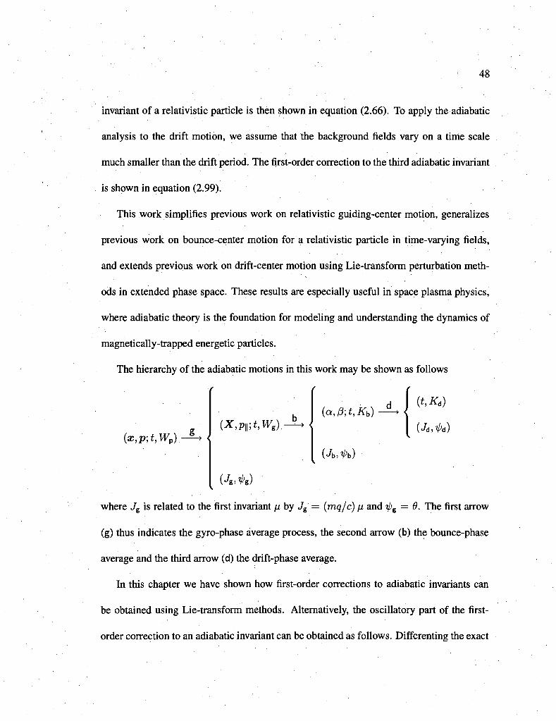
The hierarchy of the adiabatic motions in this work may be shown as follows

(x,p;t,Wp) -+ <

(X,pr,t,Wg) - <

(t,Kd)

where J% is related to the first invariant // by Jg = {mq/c) /J, and ipg = 6. The first arrow

(g) thus indicates the gyro-phase average process, the second arrow (b) the bounce-phase

average and the third arrow (d) the drift-phase average.

In this chapter we have shown how first-order corrections to adiabatic invariants can

be obtained using Lie-transform methods. Alternatively, the oscillatory part of the first-

order correction to an adiabatic invariant can be obtained as follows. Differenting the exact

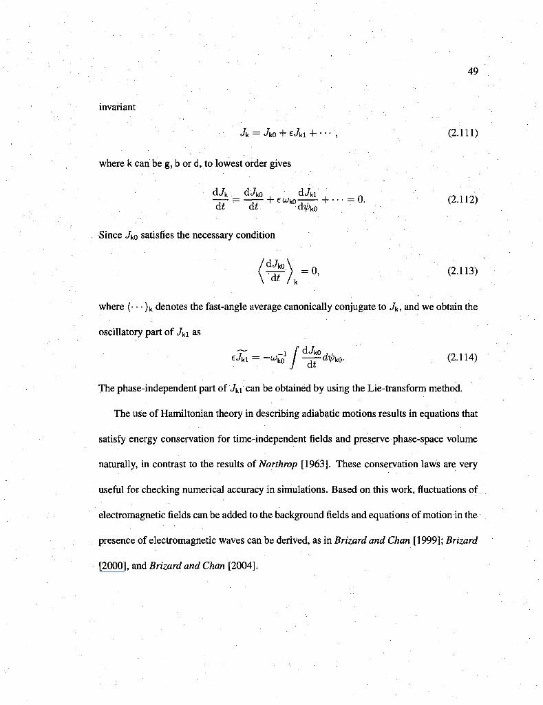
49

invariant

A =Vko + eJki .+ ••••, (2.111)

where k can be g, b or d, to lowest order gives

dJk dJk0 dJkl

-77---rr-l-ewko-T-—+ --- = 0. (2.112) dr dr d^o

Since Jko satisfies the necessary condition

'dJk0

dt , k = 0, (2.113)

where (•'• • )k denotes the fast-angle average canonically conjugate to Jk, and we obtain the

oscillatory part of Jki as

eJkl = —0/y,1 / ^^<# k o- (2.114) dJko dt

The phase-independent part of Jki can be obtained by using the Lie-transform method.

The use of Hamiltonian theory in describing adiabatic motions results in equations that

satisfy energy conservation for time-independent fields and preserve phase-space volume

naturally, in contrast to the results of Northrop [1963]. These conservation laws are very

useful for checking numerical accuracy in simulations. Based on this work, fluctuations of

electromagnetic fields can be added to the background fields and equations of motion in the

presence of electromagnetic waves can be derived, as in Brizard and Chan [1999]; Brizard

[2000], and Brizard and Chan [2004].

Chapter 3

Stochastic modeling of

multi-dimensional diffusion in the

radiation belts

This chapter has been published in Journal of Geophysical Research [Tao et ah, 2008].

3.1 Introduction

The Earth's outer radiation belt is very dynamic, and electron fluxes can vary by several

orders of magnitude during storm times, which makes it very hazardous to spacecrafts and

astronauts [e.g., Baker et ah, 1997]. Quasilinear diffusion theory has been used to evaluate

dynamic changes of particle fluxes in the radiation belts [Albert, 2004; Albert and Young,

2005; Home and Thome, 2003; Home et ah, 2003]. Using the quasilinear diffusion theory

50

51

to model radiation belt dynamics requires at least two kinds of computations: numerical

solution of a diffusion equation, which is a one-dimensional or multi-dimensional Fokker-

Planck equation, depending on diffusion processes we are interested in, and calculation of

diffusion coefficients.

Albert [2004] has shown that numerical problems arise when applying standard finite

difference methods to pitch-angle and energy diffusion equations, because of rapidly vary­

ing off-diagonal diffusion coefficients. Albert and Young [2005] developed a method for

solving the 2D diffusion equation which diagonalizes the diffusion tensor by transforming

to a new set of coordinates and solves the transformed equation by simple finite difference

methods. In this work we introduce another method, which uses probabilistic representa­

tions of solutions of Fokker-Planck equations [Freidlin, 1985; Costantini et al, 1998] via

stochastic differential equations (SDEs) and we develop a 2D code for solving pitch-angle

and energy diffusion equations. Compared with finite difference methods, the SDE method

has three main advantages. First, the SDE method is very efficient when solutions on only

a small number of points are desired, particularly when applied to high-dimensional prob­

lems, and it is easy to code and parallelize, with parallelization efficiency close to one.

Second, with the SDE method we are able to handle complicated boundary geometry, other

than constant-coordinate boundaries (see section 3.2.2). Third, generalization of the SDE

method to higher dimensions is straightforward and we expect the method to be applicable

to general 3D radiation belt diffusion equations. For more applications of similar meth­

ods using relations between Fokker-Planck equations and SDEs, see, e.g., Zhang [1999];

52

Albright et al. [2003]; Alanko-Huotari et ah [2007]; Qin et al. [2005] and Yamada etui.

[1998].

Besides solving diffusion equations, correctly calculating quasilinear diffusion coef­

ficients is also important for numerical modeling of the radiation belt dynamics using

quasilinear theory. Albert [2005] and Glauert and Home [2005] have shown full calcu­

lations of diffusion coefficients for cyclotron resonant wave-particle interactions, where

up to n = ±5 resonances are included. However, the full calculation of diffusion coef­

ficients is very time consuming. Summers [2005] derived simplified formulae for coeffi­

cients with a parallel-propagation approximation (and hence only the n = —1 resonance is

included), and the computation becomes much faster. Shprits et al. [2006c] calculated

bounce-averaged pitch-angle and energy diffusion coefficients Daoao and Dw with the

parallel-propagation approximation for E < 1 MeV particles, and compared them with

fully calculated coefficients from the PADIE code of Glauert and Home [2005]. They

concluded that coefficients for field-aligned waves are close to coefficients for waves with

mildly oblique wave normal angle distribution from the PADIE code. However, using the

wave model from Home et al. [2005], we compute particle fluxes and we show that for

E = 2 MeV electrons, Daoao and Dm calculated with the parallel-propagation approx­

imation produce flux differences of about one order of magnitude at some pitch angles,

compared to using fully calculated coefficients. Furthermore, we show that by including

off-diagonal terms in the calculation, the parallel propagation approximation also produces

large errors in fluxes for both E = 0.5 MeV and 2 MeV electrons at small pitch angles.

' 53

The remainder of this chapter is organized as follows. The SDE method and its nu­

merical implementation are introduced in section 3.2. In section 3.3 we present the ap­

plication of the SDE method to a bounce-averaged radiation belt pitch-angle and energy

diffusion equation. After describing the implementation of the SDE method for the pitch-

angle-energy equation (section 3.3.1), we show comparisons between results from the SDE

method and the Albert and Young [2005] transformation method (section 3.3.2). Then

fluxes calculated from diffusion coefficients with the parallel-propagation approximation

[Summers, 2005] are compared with fluxes computed with coefficients from full quasilin-

ear theory [Albert, 2005] (section 3.3.3). We summarize our work and discuss future work

in section 3.4.

3.2 The SDE method

Our SDE code is based on mathematical results which show that solutions of diffusion

equations can be obtained using an equivalent stochastic process. Thus we first give a de­

scription of a stochastic process using Ito stochastic differential equations in section 3.2.1.

Then we show how these lead to probabilistic representations of solutions of diffusion

equations in section 3.2.2.

3.2.1 ltd stochastic differential equations

Stochastic differential equations (SDEs) are used to describe stochastic processes. They

differ from ordinary differential equations by having terms involving random variables

54

[Gardiner, 1985; Freidlin, 1985]. A general m-dimensional SDE with a n-dimensional

Wiener process is written as

dX(t)=b(X,t)dt + (r(X,t)dW{t), (3.1)

where the m-vector X represents an m-dimensional stochastic process (Xi, X2, • • • , Xm).

Throughout this work, stochastic processes are indicated by uppercase characters, and their

values at a given time are represented by corresponding lower case characters. The n-vector

W is a n-dimensional Wiener process (Wi, W2, ••• , Wn) and dW(t) = W(t+dt) -W(t)

[Gardiner, 1985]; an increment of a one-dimensional Wiener process is proportional to

a Gaussian random number. The m-vector b and the m x n matrix cr are coefficients

that determine the values of X(i), they will be directly related to the coefficients of a

corresponding diffusion equation in section 3.2.2. Stepping equation (3.1) in time generates

a random walk trajectory through X space.

Note that SDEs may be formulated using two main mathematical methods, the Ito

method and the Stratonovich method [Gardiner, 1985]. In this work we use Ito SDEs,

because they are directly related to diffusion equations of interest for the radiation belts,

and they are mathematically more convenient [Oksendal, 1992; Freidlin, 1985; Costantini

etal, 1998].

3.2.2 Probabilistic representation of solutions of diffusion equations

To solve a diffusion equation using SDEs, we can first write the diffusion equation in

Fokker-Planck form, and then obtain equivalent "time-forward" SDEs from the diffusion

55

equation. These time-forward SDEs can then be used to simulate particle trajectories us­

ing a Monte Carlo technique, and the distribution of particles at any given time can be

obtained by binning particles in phase space. This time-forward SDE method is presented

in Appendix A to show local effects of off-diagonal terms on the distribution of particles.

Alternatively, in this section we present a "time-backward" SDE method, where solutions

of diffusion equations are represented by the mean value of a functional of trajectories

of a stochastic process [Freidlin, 1985]. This is the method used in our current SDE code.

Compared with the time-forward method, the time-backward method is more efficient when

solutions on fewer points are of interest, and it is better for handling a variety of boundary

conditions.

To introduce the time-backward SDE method, let us first consider a d-dimensional dif­

fusion equation written as

+ f*bi(t,y)^(t,*) + c(tix.)f{t,x), (3.2) tt dxi

with initial and Dirichlet boundary conditions

/(0,x) = 2o(x), xe£>, (3.3)

/( i ,x) = <?i(i,x), x e d £ > . (3.4)

Here D is the domain of the problem with boundary dD, and <7i(0,x) = go(x) on dD.

Note that dD is not restricted to constant-coordinate surfaces in the SDE method [Frei­

dlin, 1985].The solution /(x, t) of equation (3.2) is related to the following d-dimensional

56

stochastic process

dX(s) = b(t-s,X)ds + (r(t-s,X)dW(s), 0<s<t, (3.5)

where X(s = 0) = x, and W(s) is a d-dimensional Wiener process. Here the d x d matrix

<T is defined by acrT = a. Note that a is not uniquely determined by this equation, but

according to Levy's theorem [Zhang, 1999; Freidlin, 1985] different choices of a generate

equivalent stochastic processes that yield the same solution of the diffusion equation (3.2).

Also note that equation (3.5) is a time-backward SDE: at s = 0, we evaluate b and CT at time

t, while at s = t, we evaluate b and a at time 0. The solution / (x, t) is then represented

by the stochastic process defined in equation (3.5) as

; / ( x , t ) = E(FX), (3.6)

where E denotes the expectation value, and Fx is defined by

I 9b(X|a=t) exp(y|s=t), r>t\

(3.7)

£i(£-T,X|s=T)exp(Y|s=T), • r<t, where r has the value of s when the stochastic process X(s) exits from the boundary 3D for the first time, and Y(s) is defined by

Y{s) = f c(t - r,X(r))dr. (3.8)

Jo

Numerical calculation of / can be constructed easily from equations (3.6)-(3.8): To

obtain / (x , i ) , we sample a number of trajectories of the stochastic process defined by

equation (3.5) starting from x and s = 0, using a Monte-Carlo technique. The simulation of

57

a trajectory will stop either by reaching the initial condition at s = t (where time = 0) or by

reaching the boundary of the domain D at s = r, whichever comes first, and returns a value

defined by equation (3.7). Then we use the average of values returned by all trajectories to

approximate / (x, t). This process is repeated if we want to calculate / at other points.

Now let us also consider a particular type of Neumann boundary condition that is com­

monly encountered in radiation belt diffusion equations:

V / - n = 0, xediD, (3.9)

where V / = (df/dx1, df/dx2, • • • , df/dxd), the boundary d\D is the part of 3D with

the Neumann condition, and n is the inward unit normal vector on d\D. General methods

for implementing Neumann boundary conditions in SDE solutions can be found in Frei-

dlin [1985] and Costantini et al. [1998]; here we simply note that condition (3.9) can be

enforced in our numerical calculation of /(x, t) as follows: Every time a trajectory reaches

the Neumann boundary d\D, we immediately reflect it about the normal vector n [Bossy

et al., 2004]. This trajectory will later be stopped by either reaching the initial condition or

a Dirichlet boundary and at that time the trajectory returns a value defined by equation (3.7).

3.3 Application

In this section, we apply the above SDE method to a bounce-averaged pitch-angle and

energy diffusion equation [Albert, 2004]. In section 3.3.1 we derive the stochastic process

used to solve the diffusion equation. In section 3.3.2 fluxes calculated using the SDE code

58

are compared with results from Albert and Young [2005] to show that the SDE code is

capable of solving the diffusion equation with off-diagonal diffusion coefficients. To show

the effect of diffusion coefficients with the parallel-propagation approximation [Summers,

2005] on particle fluxes, we solve the diffusion equation using these diffusion coefficients

and in section 3.3.3 we compare with results obtained using fully calculated coefficients.

3.3.1 Application to pitch-angle and energy diffusion equations

We apply the above SDE method to the bounce-averaged pitch-angle and energy diffusion

equation written in equatorial pitch angle and momentum (a0, p)

21 A-JLr(n \2L n 21 dt ~ Gpdao \ aoaopda0

+ aoPdp

LJLrfn -^L n 21 GdpG{ aoPpda0

+Dppdp + ^—G(DaoP-^- + Dpp-^-), (3.10)

where Daoao, DaoP and Dpp are bounce-averaged pitch-angle, mixed and momentum diffu­

sion coefficients [Albert, 2004]. Here G is a Jacobian factor, G = p2T(a0) sin(a0) cos(a0).

and T(a0) « 1.30 — 0.56sin(ao) is the normalized bounce period. Initial and boundary

conditions are chosen to be the same as in Albert and Young [2005]. Thus the initial flux is

j(t = 0) = exp[—(E — 0.2)/0.1][sin(a0) — sin(a0z,)], where the loss cone angle a0L = 5°

59

and flux j is related to phase-space density / by j = f/p2. Boundary conditions are

/L=*o, = .0. -(3:11)

df_ da0

= 0, (3.12) Q0=90°

/ I M ™ = °> 0.13)

where i?min = 0.2 MeV and .E^a* = 5 MeV, and pmin is the momentum corresponding to

Emin [Albert and Young, 2005].

To solve the equation using the time-backward SDE method, we first write equation

(3.10) in the form of (3.2); i.e.,

df _ Daoaod*f ( 2Daop d2f d'f dt p2 dal p da0dp ndp2

with

w'.*.rt = ^ ( r i r H I O ^ ) ' (3i« 1 d {GDaoao\ Id (GDaoP

p ) + C I d , , 18

bp(t,a0,p) = — — {GDaop) + --^{GDvp). (3.17)

Thus the two-dimensional stochastic process defined in equation (3.5) becomes

dA0(s) = bao(t—s,A0,P)ds + audWi + <Ti2dW2,- (3.18)

dP(s) = \(t-s,Ao,P)ds + a2idWi +<T*2dW2, (3.19)

with Ao(s = 0) = ao and P(s = 0) = p. Then, because of the Neumann boundary

condition at a0 = 90°, we numerically reflect A0 with respect to a0 = 90° if it is larger

60

than 90°. Here components of the matrix a are defined by

/

V O21 <T22

e n cr2i

/ V C 1 2 (J22 /

\ 2Daoao/p

2 2Daop/p

^ 2Daop/P ^Dpp J

(3.20)

In this work, we choose au — 0 for simplicity and then the other components are

On

022

y/2Dao<xo/P >

V2Daop/^D, aoao ;

-V ^•L^rvn PP U 2 1 »

(3.21)

(3.22)

(3.23)

where we have used the fact that Dao0lQ is never zero in equation (3.22).

We have developed a 2D SDE code to solve the diffusion equation (3.10), where SDEs

(3.18) and (3.19) are integrated using the Euler-Maruyama method [Kloeden and Platen,

1992]. That is,

A0(sn+i) = A0(sn) + bao[t-sn,A0(sn),P(sn)] As

+ an{sn) AW! + ) AW2,

P(sn+1) = P{sn) + bp[t-sn,A0(sn),P(sn)}As

&22\Sn )AW2.

(3.24)

(3.25)

Here AW = -\/sn+i — snN(0,1), where N(0,1) is a standard Gaussian random number

with zero mean and unit variance, generated using the Box-Muller algorithm [Press et ah,

2002]. Because the original time-backward SDE method requires fresh samples of trajec­

tories for every different (ato,p) and traces trajectories back to the initial condition or to a

61

boundary every time, the current SDE code is less efficient when solutions on many grid

points for long times are needed. Improving the efficiency of the SDE code is one of tasks

in our future work. In this work, we mainly want to show that the method can be used

to solve multi-dimensional diffusion equationsi Results from the SDE code are compared

with Albert and Young [2005] in the next section.

3.3.2 Comparisons with Albert and Young [2005] results

Albert and Young [2005] solve the diffusion equation (3.10) by first transforming to new

coordinates which diagonalize the diffusion tensor, and then applying standard finite dif­

ference methods to the transformed diffusion equation. The bounce-averaged diffusion

coefficients Daoao,Daop,Dm for storm-time chorus waves were calculated at L = 4.5,

with computational methods of Albert [2005]. The wave model used to calculate diffusion

coefficients is described in Home et al. [2005] and Albert and Young [2005]; the wave mag­

netic field is given by J5^ = B2(u;)<k,(tan 6), where the wave power spectral density B2(u>)

and the wave normal angle (tan#) distribution function ^(tanfl) are truncated Gaussian

functions defined between lower and upper frequency cutoffs (UJLC < w < <^uc) and wave

normal angle cutoffs (QLC < 0 < Que)- The latitudinal distribution of the waves and the

ratio of electron plasma frequency (/pe) to electron cyclotron frequency (/ce) are the same

as those used by Home et al. [2005] and Albert and Young [2005] and are shown in Table

3.1. Similar models were used by Li et al. [2007]. Up to n = ±5 resonance harmonics were

included in the calculation. The calculated diffusion coefficients Daoao are proportional to

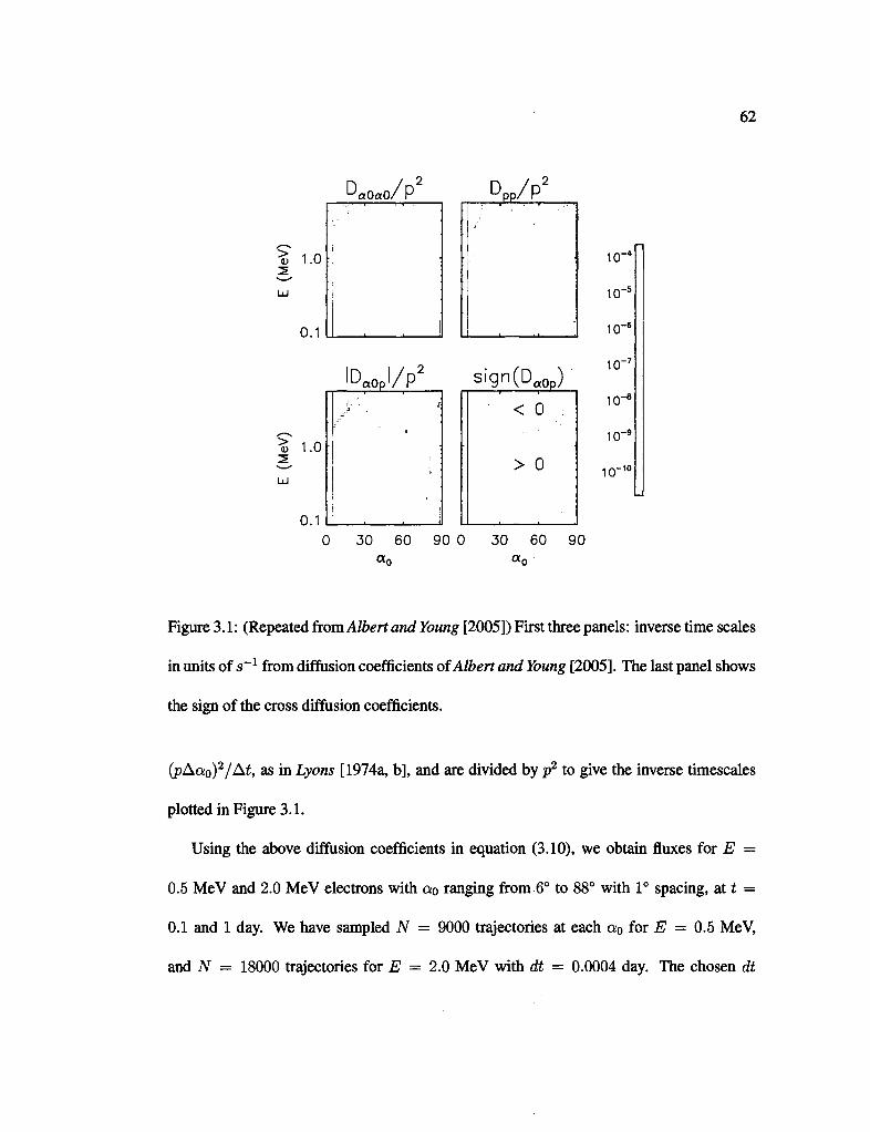
62

D«o«o/p2 Dpp/P2

• ^ - T T — ^ - i — - — i i i " " ! 1 " r r ^ ' — ~ n

10-4

! 1CT5

• • I l l , . J 1 0 - 6

10~7

lD«opl/p2 sign(Dgop) \

10-8

10"9

0 30 60 90 0 30 60 90

Figure 3.1: (Repeated from Albert and Young [2005]) First three panels: inverse time scales

in units of s - 1 from diffusion coefficients of Albert and Young [2005]. The last panel shows

the sign of the cross diffusion coefficients.

(pAa0)2/At, as in Lyons [1974a, b], and are divided by p2 to give the inverse timescales

plotted in Figure 3.1.

Using the above diffusion coefficients in equation (3.10), we obtain fluxes for E —

0.5 MeV and 2.0 MeV electrons with ao ranging from 6° to 88° with 1° spacing, at t —

0.1 and 1 day. We have sampled N = 9000 trajectories at each a0 for E = 0.5 MeV,

and N = 18000 trajectories for E = 2.0 MeV with dt = 0.0004 day. The chosen dt

^ 1.0

0.1

$ 1.0

0.1

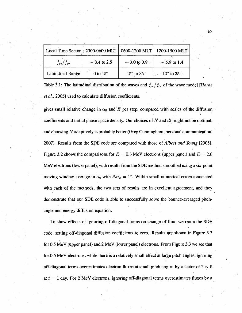
63

Local Time Sector

J pelJce

Latitudinal Range

2300-0600 MLT

~ 3.4 to 2.5

0tol5°

0600-1200 MLT

~ 3.0 to 0.9

15° to 35°

1200-1500 MLT

~ 5.9 to 1.4

10° to 35°

Table 3.1: The latitudinal distribution of the waves and fpe/fce of the wave model [Home

et ah, 2005] used to calculate diffusion coefficients.

gives small relative change in a0 and E per step, compared with scales of the diffusion

coefficients and initial phase-space density. Our choices of N and dt might not be optimal,

and choosing N adaptively is probably better (Greg Cunningham, personal communication,

2007). Results from the SDE code are compared with those of Albert and Young [2005].

Figure 3.2 shows the comparisons for E = 0.5 MeV electrons (upper panel) and E = 2.0

MeV electrons (lower panel), with results from the SDE method smoothed using a six-point

moving window average in a0 with Aa0 = 1°. Within small numerical errors associated

with each of the methods, the two sets of results are in excellent agreement, and they

demonstrate that our SDE code is able to successfully solve the bounce-averaged pitch-

angle and energy diffusion equation.

To show effects of ignoring off-diagonal terms on change of flux, we rerun the SDE

code, setting off-diagonal diffusion coefficients to zero. Results are shown in Figure 3.3

for 0.5 MeV (upper panel) and 2 MeV (lower panel) electrons. From Figure 3.3 we see that

for 0.5 MeV electrons, while there is a relatively small effect at large pitch angles, ignoring

off-diagonal terms overestimates electron fluxes at small pitch angles by a factor of 2 ~ 5

at t = 1 day. For 2 MeV electrons, ignoring off-diagonal terms overestimates fluxes by a

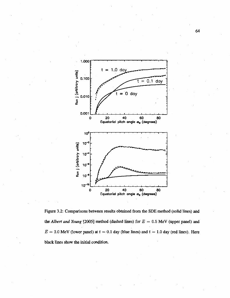
64

0.001 20 40 60 80

Equatorial pitch angle a0 (degrees)

.tr E 3

e* >

:i :s j j .

X

= C

10"

10"2

10-4

10"6

io-8

10-10

if

y^0^^

—i 1 1 1 1 1 1 1 1 1 r

^ ^ ^ ^ ^ s

1 '

-

B-W"—NC

.-

-

, 0 20 40 60 80

Equatorial pitch angle a0 (degrees)

Figure 3.2: Comparisons between results obtained from the SDE method (solid lines) and

the Albert and Young [2005] method (dashed lines) for E = 0.5 MeV (upper panel) and

E = 2.0 MeV (lower panel) at t = 0.1 day (blue lines) and t .= 1.0 day (red lines). Here

black lines show the initial condition.

65

factor of 5 ~ Watt = 1 day, with larger errors at smaller pitch angles. Thus off-diagonal

terms are more important for 2 MeV electrons We emphasize that these results are for the

Home et al. [2005] wave model, and we note that the peak in flux of 2 MeV electrons near

30° may be related to the cutoff in wave power at 35° latitude in the Home et al. [2005]

model (see discussion in section 3.4).

3.3.3 Effects of parallel propagation approximation

Summers [2005] and Summers et al. [2007a, b] have derived cyclotron-resonance diffu­

sion coefficients for field-aligned waves, where only the n = — 1 resonance is included

(henceforth denoted by D^). This assumption of parallel propagation greatly improves

the computation efficiency. Bounce-averaged D" are given and compared with diffusion

coefficients obtained from the PADIE code [Glauert and Home, 2005] in Shprits et al.

[2006c]. In the present work, we also calculate D'l using the methods of Albert [2005],

with wave parameters the same as the wave model described in Section 3.3.2, except that

0LC = 0UC = 0. The resulting diffusion coefficients are the same as those obtained from

the PADIE code, and are half of those given by Summers et al. [2007a] (this factor of two

difference is discussed in [Albert, 2007]).

Figure 3.4 shows inverse timescales from diffusion coefficients with the parallel wave

approximation. Compared with Figure 3.1, we see that the general behavior of D" is quite

good, with larger differences for E > 1 MeV electrons. The off-diagonal terms of D" are

worse approximations than the diagonal terms, with details discussed in Albert [2007].

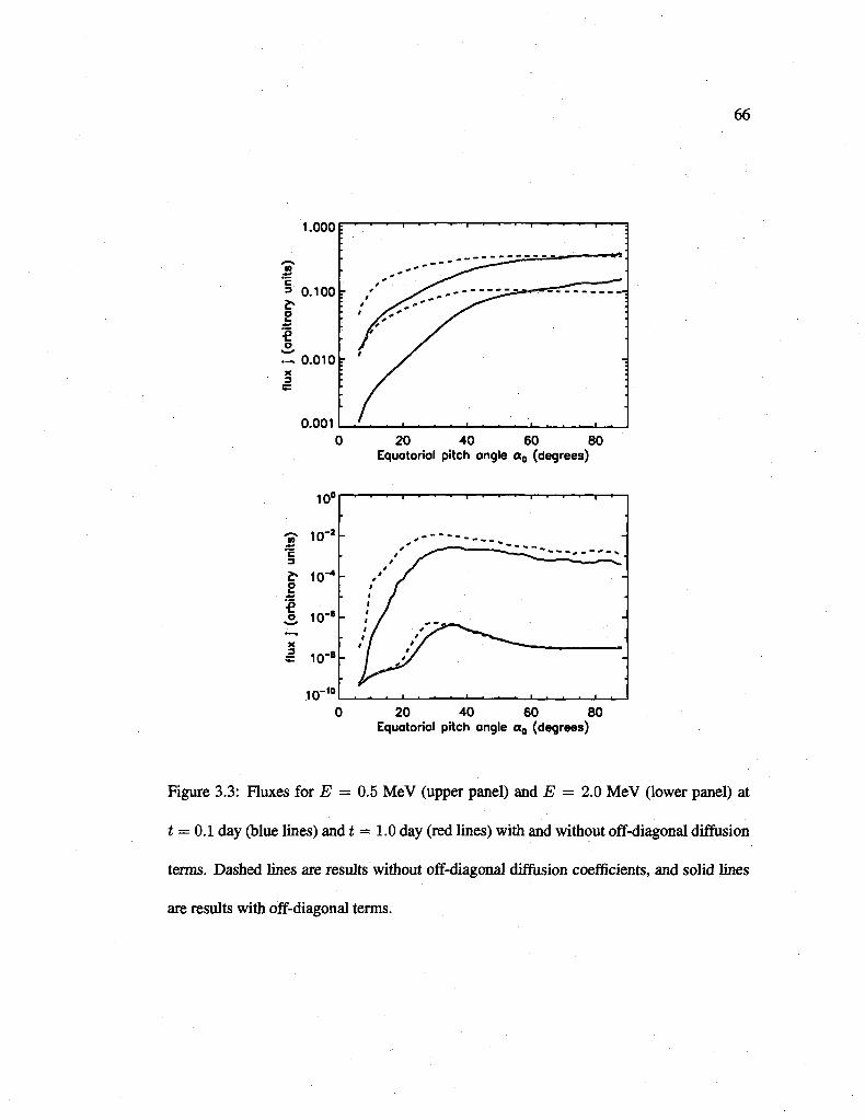
66

1.000 f

0.001 20 40 60 80

Equatorial pitch angle a0 (degrees)

0 20 40 60 80 Equatorial pitch angle a0 (degrees)

Figure 3.3: Fluxes for E = 0.5 MeV (upper panel) and E = 2.0 MeV (lower panel) at

t = 0.1 day (blue lines) and t = 1.0 day (red lines) with and without off-diagonal diffusion

terms. Dashed lines are results without off-diagonal diffusion coefficients, and solid lines

are results with off-diagonal terms.

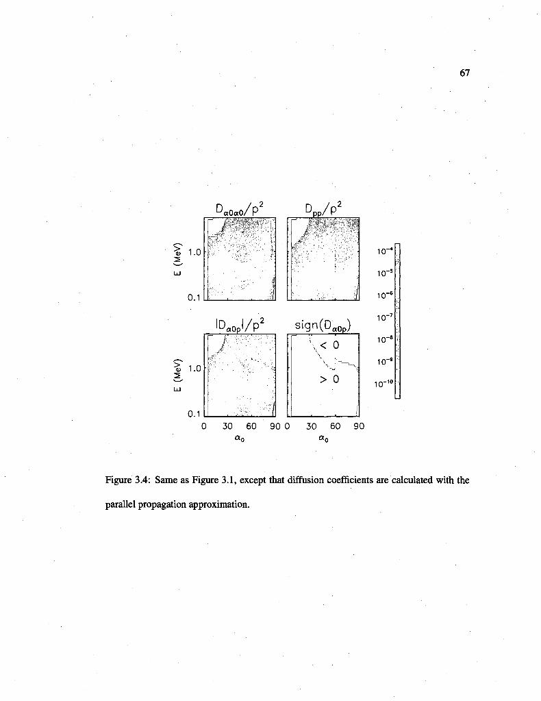
67

D«o«o/P

•' 'J I ' . I ."" .'

sign(Da0p)

r \ < o

> 0

. . 1

10"4

10"5

10"e

icr7

10"8

10"9

io-10

0 30 60 90 0 30 60 90

a„ a„

Figure 3.4: Same as Figure 3.1, except that diffusion coefficients are calculated with the

parallel propagation approximation.

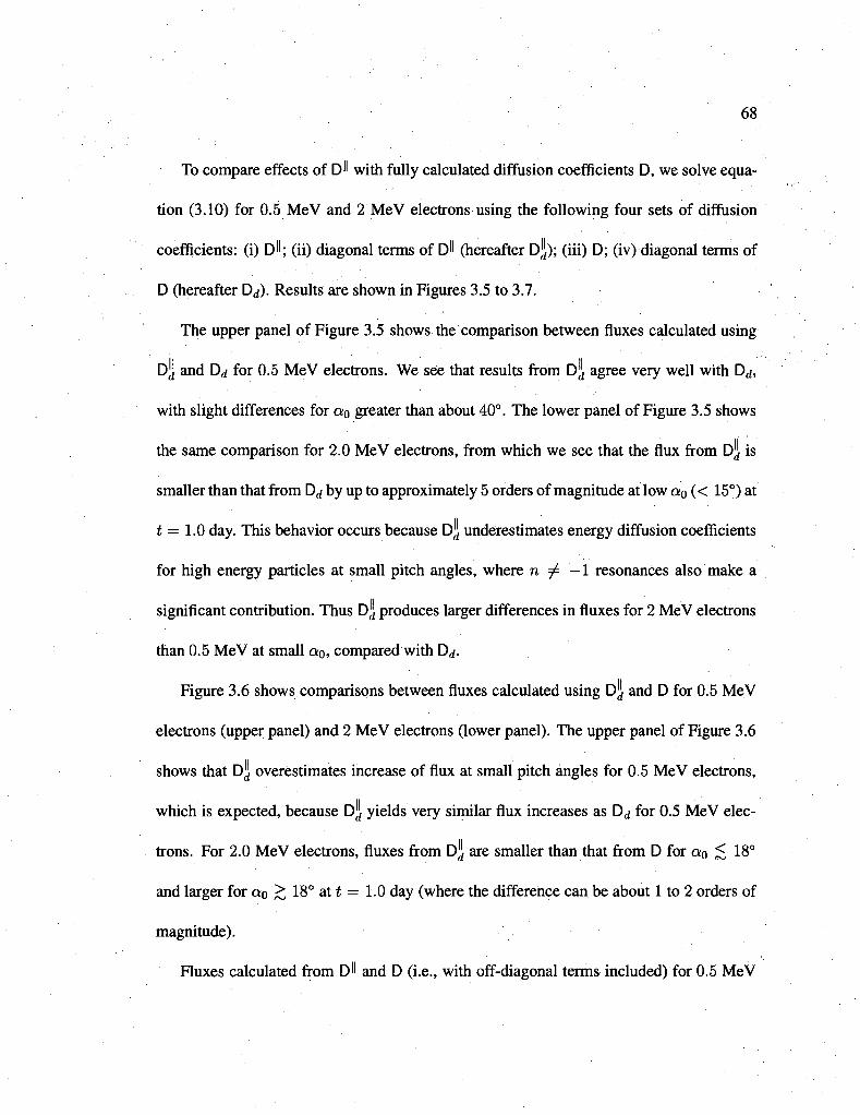
68

To compare effects of D" with fully calculated diffusion coefficients D, we solve equa­

tion (3.10) for 0.5 MeV and 2 MeV electrons using the following four sets of diffusion

coefficients: (i) D"; (ii) diagonal terms of D" (hereafter DJj); (iii) D; (iv) diagonal terms of

D (hereafter D^). Results are shown in Figures 3.5 to 3.7.

The upper panel of Figure 3.5 shows the comparison between fluxes calculated using

DJJ and D^ for 0.5 MeV electrons. We see that results from D\ agree very well with D ,

with slight differences for a0 greater than about 40°. The lower panel of Figure 3.5 shows

the same comparison for 2.0 MeV electrons, from which we see that the flux from DJj is

smaller than that from D^ by up to approximately 5 orders of magnitude at low a0 (< 15°) at

t = 1.0 day. This behavior occurs because DJj underestimates energy diffusion coefficients

for high energy particles at small pitch angles, where n ^ — 1 resonances also make a

significant contribution. Thus DJj produces larger differences in fluxes for 2 MeV electrons

than 0.5 MeV at small a0, compared with D<*.

Figure 3.6 shows comparisons between fluxes calculated using DJj and D for 0.5 MeV

electrons (upper panel) and 2 MeV electrons (lower panel). The upper panel of Figure 3.6

shows that DJj overestimates increase of flux at small pitch angles for 0.5 MeV electrons,

which is expected, because Dj| yields very similar flux increases as D^ for 0.5 MeV elec­

trons. For 2.0 MeV electrons, fluxes from DJ| are smaller than that from D for a0 < 18°

and larger for a0 > 18° at t = 1.0 day (where the difference can be about 1 to 2 orders of

magnitude).

Fluxes calculated from D" and D (i.e., with off-diagonal terms included) for 0.5 MeV

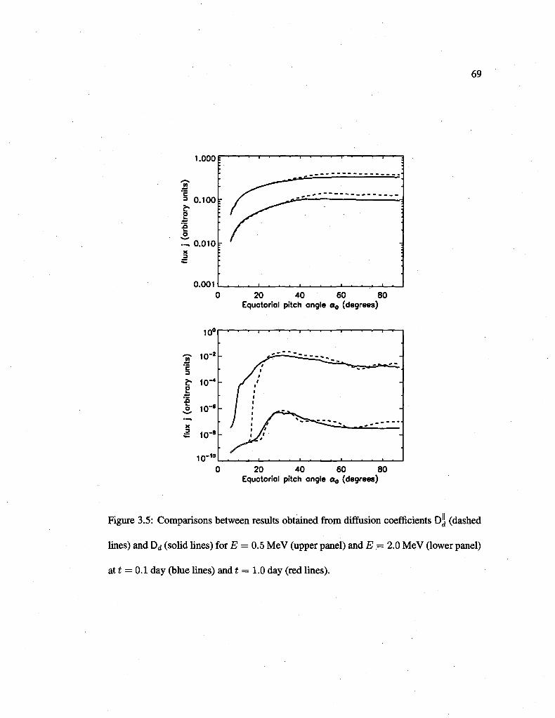
69

1.000

0.001 0 20 40 60 80

Equatorial pitch angle a0 (degrees)

20 40 60 80 Equatorial pitch angle a0 (degrees)

Figure 3.5: Comparisons between results obtained from diffusion coefficients Dj[ (dashed

lines) and Dd (solid lines) for E = 0.5 MeV (upper panel) and E — 2.0 MeV (lower panel)

at t — 0.1 day (blue lines) and t — 1.0 day (red lines).

70

1.000b • ' '

0.001

• • • • • • i l l

0 20 40 60 80 Equatorial pitch angle a0 (degrees)

0 20 40 60 80 Equatorial pitch angle a0 (degrees)

Figure 3.6: Comparisons between results obtained from diffusion coefficients D\ (dashed

lines) and D (solid lines) for E = 0.5 MeV (upper panel) and E = 2.0 MeV (lower panel)

at t = 0.1 day (blue lines) and t = 1.0 day (red lines).

71

(upper panel) and 2 MeV (lower panel) electrons are shown in Figure 3.7. Reasonable

agreement between D" and D fluxes is obtained for a0 > 50°, but significant differences

occur at smaller pitch angles. For 0.5 MeV electrons, D" underestimates increases of flux

at t — 1.0 day by approximately an order of magnitude for a0 < 20°. For 2.0 MeV

electrons, behavior of D is worse at t == 1.0 day. We see from the lower panel of Figure

3.7 that D'l underestimates increases of flux by approximately 1 ~ 4 orders of magnitude

for 10° < a0 < 35°. Thus the approximation of parallel propagation produces larger

differences at small pitch angles for higher energy particles, especially when off-diagonal

terms are included.

3.4 Summary and discussion

In this work a new code, based on the mathematical theory of expressing solutions of

diffusion equations in terms of related stochastic processes, has been developed for solving

multi-dimensional radiation belt diffusion equations. Two examples are used to show its

applications.

First, we apply the SDE code to a bounce-averaged pitch-angle and energy diffusion

equation and obtain excellent agreement with a previously developed method [Albert and

Young, 2005]. We also confirm that ignoring off-diagonal terms in the diffusion equation

overestimates increase of flux, especially at small pitch angles, at t = 1 day (by a factor of

2 ~ 5 for 0.5 MeV, and 5 ~ 10 for 2 MeV electrons) using the Albert and Young [2005]

diffusion coefficients.

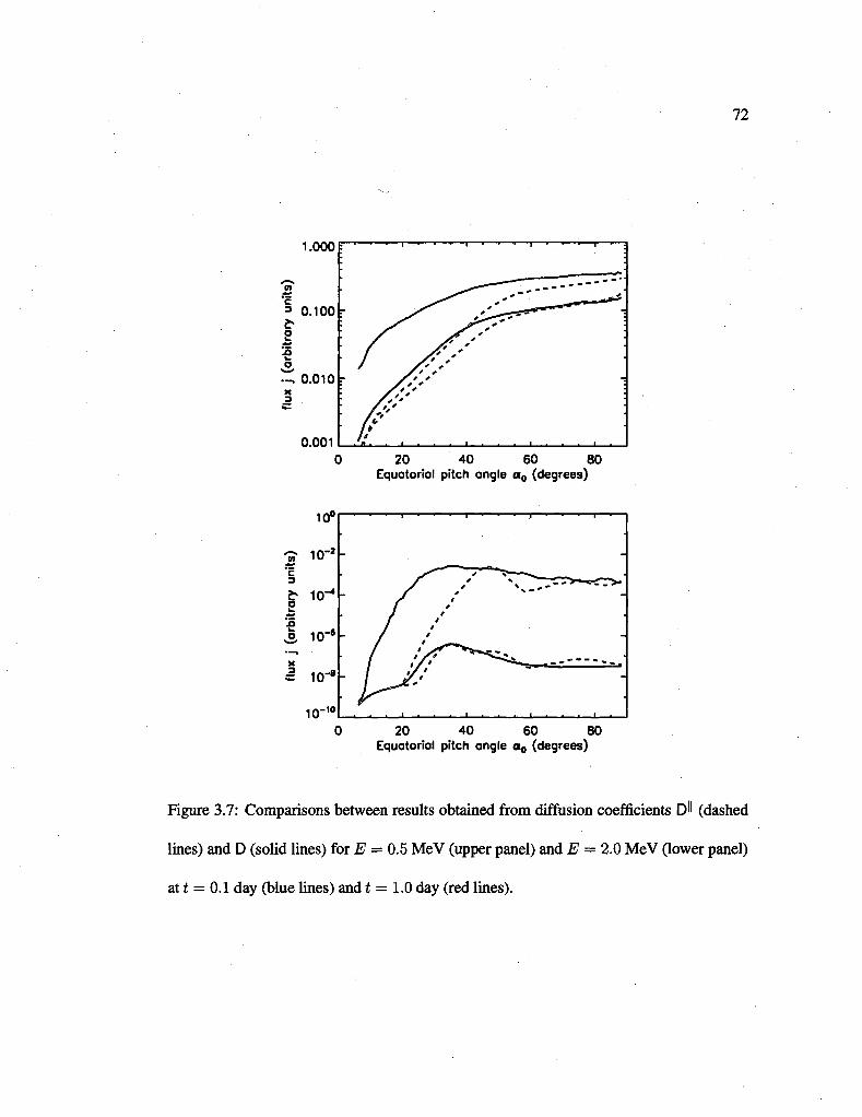
72

1.000

0.001 0 20 40 60 80

Equatorial pitch angle a0 (degrees)

10"

(arb

itrar

y un

its)

o

o

o

X

i io-8

io-10

1.

1.

1 — i i 1 1 • |

/ / y / / / / / / /

• i j • y • | •

^ ^ ^ j » ^ a> «• — v _

-

i i - . . . i •— * > _ i .

0 20 40 60 80 Equatorial pitch angle a0 (degrees)

Figure 3.7: Comparisons between results obtained from diffusion coefficients D" (dashed

lines) and D (solid lines) for E = 0.5 MeV (upper panel) and E = 2.0 MeV (lower panel)

at t = 0.1 day (blue lines) and t = 1.0 day (red lines).

Second, by solving the bounce-averaged pitch-angle and energy diffusion equation us­

ing fully-calculated diffusion coefficients D [Albert and Young, 2005] and coefficients with

the parallel propagation approximation D" [Summers, 2005; Summers et ah, 2007a, b],

both calculated using the chorus wave model of Home etal. [2005], we show that diagonal

diffusion coefficients of D" agree well with that of D only for low energy particles (e.g.,

E = 0.5 MeV). For high energy electrons, the difference between the diagonal terms of D"

and D produces large differences in fluxes at some pitch angles (difference of up to 5 orders

of magnitude for 2 MeV electrons at a0 ^ 15°, at t = 1.0 day). By including off-diagonal

diffusion coefficients in our calculation, we show that the off-diagonal terms of D" can pro­

duce difference in fluxes of 4 orders of magnitude for 2 MeV electrons at t = 1.0 day. A

discussion of the details of different diffusion coefficients and another approximation for a

full calculation of diffusion coefficients are presented in Albert [2007].

Note that the above conclusions on the magnitude and location of differences that occur

by omitting off-diagonal terms and assuming parallel propagating waves are very likely to

be dependent on the wave model used. For example, a different latitudinal distribution of

wave power may result in different diffusion coefficients and thus different conclusions.

The sensitivity of our results to wave models needs further study. However, before such

work is done, it is safer to include both off-diagonal terms and oblique waves in calculations

of electron flux.

The SDE method is less efficient when solutions on many grid points are desired. How­

ever, when parallel computers are available, computation time can be greatly reduced be-

74

cause of high parallelization efficiency. Generalization to 3D is straightforward, and our

next step is to build a 3D model including pitch-angle, energy and radial diffusion using

this method. The SDE method is very promising for providing new insights into the rel­

ative roles of local acceleration and radial diffusion as acceleration mechanisms, and the

importance of pitch-angle diffusion as a loss process.

Chapter 4

Modeling of multi-dimensional diffusion

in radiation belts using layer methods

This chapter has been published in Journal of Geophysical Research [Tao et ah, 2009].

4.1 Introduction

In Chapter 3, we developed a stochastic differential equation (SDE) code to solve 2D

bounce-averaged pitch angle and energy diffusion equations. The SDE code is very ef­

ficient when solutions on a small number of points are needed. However, if solutions are

needed on a large computational domain for long times, the SDE code becomes less effi­

cient, for reasons explained in Chapter 3. Milstein [2002], Milstein and Tretyakov [2002]

and Milstein and Tretyakov [2001] have used properties of numerical integration of SDEs

to develop so-called layer methods, which are deterministic, to solve parabolic equations

75

76

successively in time. In this chapter we develop a code using layer methods and show that

it is able to solve 2D radiation belt diffusion equations with cross diffusion and it is gen-

eralizable to 3D. Although the layer code does not have the high parallelization efficiency

compared with the SDE code in Chapter 3, it is more efficient when solving the diffusion

equation over a large computational domain for long times. Also our layer code can handle

boundary conditions with complicated geometry rather than constant-coordinate bound­

aries that are typically used in finite difference codes.

Using this layer code, we then explore effects of ignoring off-diagonal terms using two

wave models: the chorus wave model from Li et al. [2007], and the combined magnetosonic

wave [Home et al, 2007] and hiss wave [Li et al, 2007] (MH) model. In Chapter 3, we

show that ignoring off-diagonal terms causes errors of an order of magnitude for 2 MeV

electrons at small pitch angles using the Home et al. [2005] chorus wave model. Using the

Liet al. [2007] chorus wave model and the MH wave model is helpful in understanding the

sensitivity of the main conclusions of Chapter 3 to different wave models.

The remainder of this chapter is organized as follows. We introduce the layer methods

by using a simple initial-value problem in section 4.2. Details of our 2D layer code to solve

a bounce-averaged pitch angle and energy diffusion equation are given in section 4.3. We

first show its agreement with Albert and Young [2005] results in section 4.3.1. Then we

solve the diffusion equation with diffusion coefficients calculated using the Li et al. [2007]

chorus wave model (section 4.3.2) and the MH wave model (section 4.3.3) to show effects

of ignoring off-diagonal terms and energization of electrons. Our results are then discussed

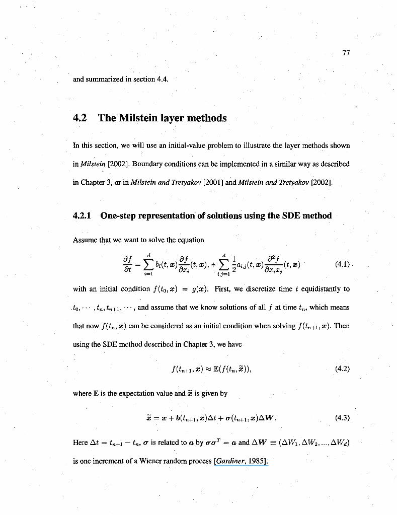
and summarized in section 4.4.

77

4.2 The Milstein layer methods

In this section, we will use an initial-value problem to illustrate the layer methods shown

in Milstein [2002]. Boundary conditions can be implemented in a similar way as described

in Chapter 3, or in Milstein and Tretyakov [2001] and Milstein and Tretyakov [2002].

4.2.1 One-step representation of solutions using the SDE method

Assume that we want to solve the equation

t=l * i,j=l l 3

with an initial condition f(t0,x) = g(x). First, we discretize time t equidistantly to

t0, • • • ,tn, tn+i, • • •, and assume that we know solutions of all / at time tn, which means

that now f(tn, x) can be considered as an initial condition when solving / (£n+i, x). Then

using the SDE method described in Chapter 3, we have

f{tn+1,x)^E(f(tn,x)), (4.2)

where E is the expectation value and x is given by

x = x + b(tn+1,x)At + cr(tn+1,x)AW. (4.3)

Here At = tn+1 - tn, cr is related to a by <rcrr = a and AW = (AWi,AW2,..., AWd)

is one increment of a Wiener random process [Gardiner, 1985].

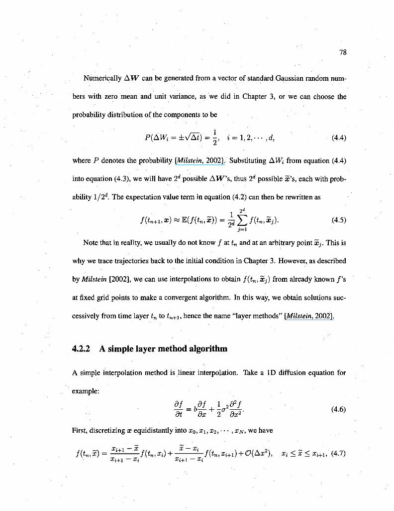
78

Numerically A W can be generated from a vector of standard Gaussian random num­

bers with zero mean and unit variance, as we did in Chapter 3, or we can choose the

probability distribution of the components to be

P{AWi = ±VKt) = \, 2 = 1,2, 2 , - -,-, ,d, (4.4)

where P denotes the probability [Milstein, 2002]. Substituting AWi from equation (4.4)

into equation (4.3), we will have 2d possible A W s , thus 2d possible x's, each with prob­

ability l/2d. The expectation value term in equation (4.2) can then be rewritten as

f(tn+ux) » E(/(in,x)) =^52/(<„,Xj). (4.5)

Note that in reality, we usually do not know / at tn and at an arbitrary point Xj. This is

why we trace trajectories back to the initial condition in Chapter 3. However, as described

by Milstein [2002], we can use interpolations to obtain f(tn, Xj) from already known / ' s

at fixed grid points to make a convergent algorithm. In this way, we obtain solutions suc­

cessively from time layer tn to tn+i, hence the name "layer methods" [Milstein, 2002].

4.2.2 A simple layer method algorithm

A simple interpolation method is linear interpolation. Take a ID diffusion equation for

example:

df _hdf , 1 2 5 2 / . -dt-bdx + 2adxf (4>6)

First, discretizing x equidistantly into xo, xi, £2, • • • , %N, we have

f(tn,x).= :Ci+iyf{tn,xi)+ X~^ f(tn,xi+1) + 0(Ax2)y Xi<x<xi+1,(^)

•^i-f-1 ^s i **si+l **si

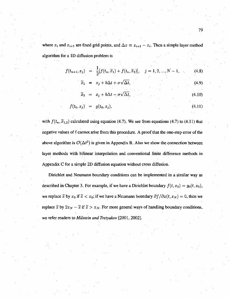
79

where x; and xi+\ are fixed grid points, and Ax = xi+i — x*. Then a simple layer method

algorithm for a ID diffusion problem is

f(tn+uXj)•=. | [ / ( t„ ,xi) + /(t„>x2)]> i = l ,2 , . . . ,7V-l , (4.8)

'•xi = Xj + 6Ai + aVAl, (4.9)

x2 = x j + bAt - aVAt, (4.10)

f(to,Xj)'. = g{t0,Xj), (4.11)

with f(tn, Xi<2) calculated using equation (4.7). We see from equations (4.7) to (4.11) that

negative values of f cannot arise from this procedure. A proof that the one-step error of the

above algorithm is 0(At2) is given in Appendix B. Also we show the connection between

layer methods with bilinear interpolation and conventional finite difference methods in

Appendix C for a simple 2D diffusion equation without cross diffusion.

Dirichlet and Neumann boundary conditions can be implemented in a similar way as

described in Chapter 3. For example, if we have a Dirichlet boundary f(t, x0) = go(t, x0),

we replace x by x0 if x < x0; if we have a Neumann boundary df/dx(t, x^) = 0, then we

replace x by 2XN — xifx> XN. For more general ways of handling boundary conditions,

we refer readers to Milstein and Tretyakov [2001, 2002].

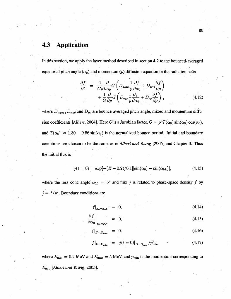
80

4.3 Application

In this section, we apply the layer method described in section 4.2 to the bounced-averaged

equatorial pitch angle (a0) and momentum (p) diffusion equation in the radiation belts

df 1 d ( ldj^ dj_

dt Gpda0 V ° °pda0 "op dp

Gdp { aoPpdaQ ^dp + T;—G [Daop-^- + Dn-£ ) , (4.12)

where Daoao, DaoP and Dpp are bounce-averaged pitch-angle, mixed and momentum diffu­

sion coefficients [Albert, 2004]. Here G is a Jacobian factor, G = p2T(a0) sin(a0) cos(o;o),

and T(a0) ~ 1.30 — 0.56sin(a0) is the normalized bounce period. Initial and boundary

conditions are chosen to be the same as in Albert and Young [2005] and Chapter 3. Thus

the initial flux is

j(t = 0) = exp[-(E - 0.2)/0.1][sin(a0) - sin(a0L)], (4.13)

where the loss cone angle a0L = 5° and flux j is related to phase-space density / by

j = f/p2. Boundary conditions are

/L=*o, = 0, (4.14)

df = 0, (4.15)

a 0 =90° da0

S\E=E^ = J(* = 0 ) | ^ m i > L n (4.17)

where Emin = 0.2 MeV and Emax = 5 MeV, andpmin is the momentum corresponding to

Em\n [Albert and Young, 2005].

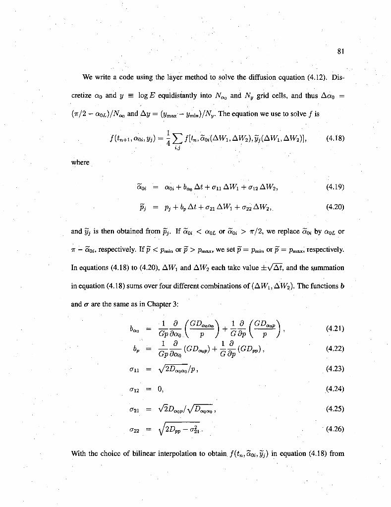
81

We write a code using the layer method to solve the diffusion equation (4.12). Dis-

cretize a0 and y = log 2? equidistantly into Nao and Ny grid cells, and thus Aa0 =

(71-/2 - aoL)/Nao and Ay = (ymax- y^/Ny. The equation we use to solve / i s

f(tn+1,aQi, Vj) = \Y, ft**' 5oi(AWi, AW2), &(AWi, AW2)], (4.18) 4

hi

where

aoi = a0i + baoAt + (7nAW1+a12AW2, (4.19)

Pj = Pj + bpAt + 0-21 AWX + a22 AW2, (4.20)

and yj is then obtained from pj. If a0i < (*OL or aQi > IT/2, we replace a0i by a0L or

7T - a0i, respectively. If p < pmin orp> praax, we set p = pmin orp = pmax, respectively.

Inequations (4.18) to (4.20), AWi and AW2 each take value ±\/A7, and the summation

in equation (4.18) sums over four different combinations of (AWi, AW2). The functions b

and a are the same as in Chapter 3:

on = ^2Daoao/p, (4.23)

an = 0, (4.24)

021 = (4.25)

22 = sJ2Dn-ulx. (4.26)

With the choice of bilinear interpolation to obtain f{tn,a0i,yj) in equation (4.18) from

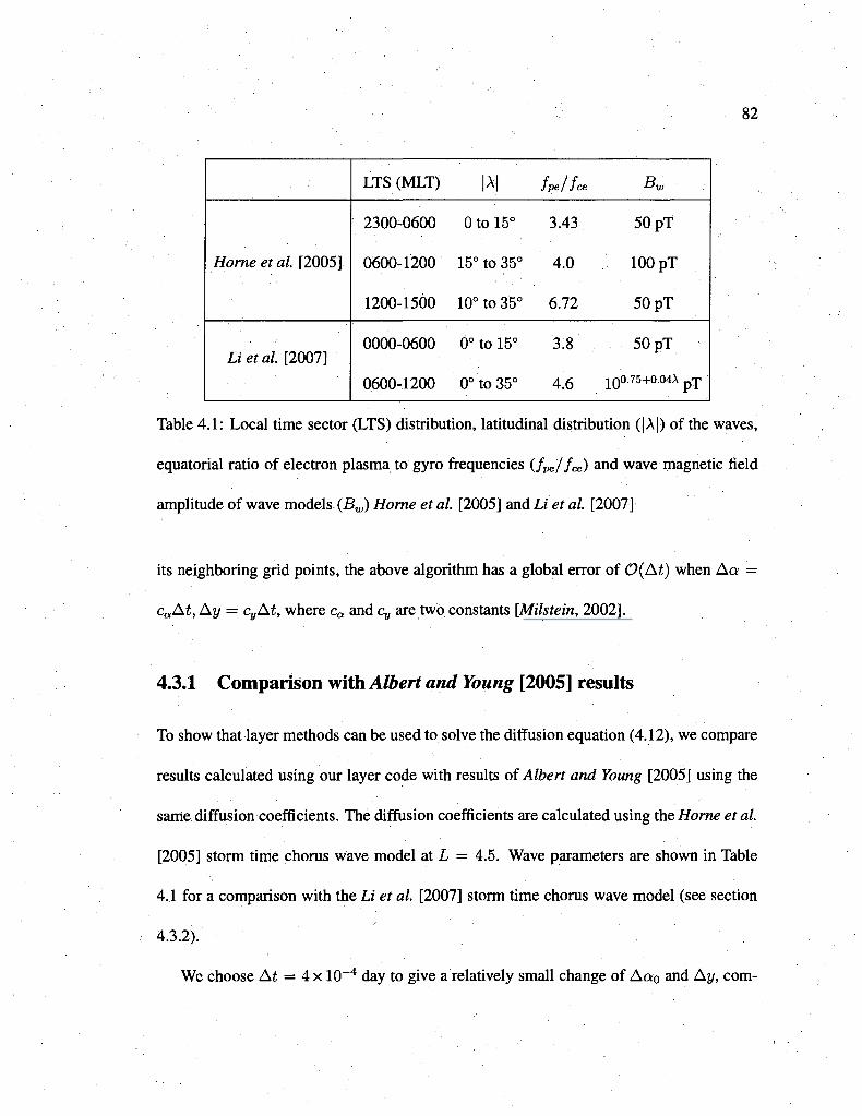
82

Home et al. [2005]

Li et al. [2007]

LTS(MLT) |AJ /pe/Zee Bw

2300-0600 0tol5° 3.43 50 pT

0600-1200 15° to 35° 4.0 100 pT

1200-1500 10° to 35° 6.72 50 pT

0000-0600 0°tol5° 3.8 50 pT

0600-1200 0°to35° 4.6 10°•75+004A pT

Table 4.1: Local time sector (LTS) distribution, latitudinal distribution (|A|) of the waves,

equatorial ratio of electron plasma to gyro frequencies (/pe//ce) and wave magnetic field

amplitude of wave models (Bw) Home etal. [2005] and Li et al. [2007]

its neighboring grid points, the above algorithm has a global error of O(At) when Aa =

caAt, Ay = cyAt, where ca and Cy are two constants [Milstein, 2002].

4.3.1 Comparison with Albert and Young [2005] results

To show that layer methods can be used to solve the diffusion equation (4.12), we compare

results calculated using our layer code with results of Albert and Young [2005] using the

same diffusion coefficients. The diffusion coefficients are calculated using the Home et al.

[2005] storm time chorus wave model at L = 4.5. Wave parameters are shown in Table

4.1 for a comparison with the Li et al. [2007] storm time chorus wave model (see section

4.3.2).

We choose At = 4 x 10-4 day to give a relatively small change of AO:Q and Ay, com-

83

pared with the computational domain. We plot fluxes of 0.5 MeV and 2 MeV at t = 2 d in

Figure 4.1 to show the convergence of solutions with respect to Nao and Ny, and this leads

to our choice of Nao — 1400 and Ny = 1500. Comparisons with results from Albert and

Young [2005] are shown in Figure 4.2 for E = 0.5 MeV (top) and E = 2 MeV (bottom)

electrons. Considering the small errors associated with each method, we conclude that the

two sets of results agree very well with each other and our layer code is capable of solving

the bounce-averaged pitch-angle and momentum diffusion equation (4.12) with cross dif­

fusion. In the next section, we apply our layer code to the diffusion equation with diffusion

coefficients calculated using the Li et al. [2007] chorus wave model.

4.3.2 Effects of ignoring cross diffusion in Li et al. [2007] chorus wave

model

Li et al. [2007] used a new chorus wave model and calculated changes of electron fluxes due

to cyclotron resonances with chorus waves by solving a 2D bounce-averaged pitch angle

and energy diffusion equation. However, cross diffusion is not included in their calculation

[Li et al, 2007]. In this work, we calculate diffusion coefficients including cross diffusion

using the Li et al. [2007] main phase storm time chorus wave model. We also use a wave

normal angle distribution from Home et al. [2005], in contrast to Li et al. [2007], who

use a parallel propagation approximation. The resulting diffusion coefficients are shown in

Figure 4.3. By solving the diffusion equation with off-diagonal terms using our layer code,

we show in this section effects of ignoring off-diagonal terms on electron fluxes using the

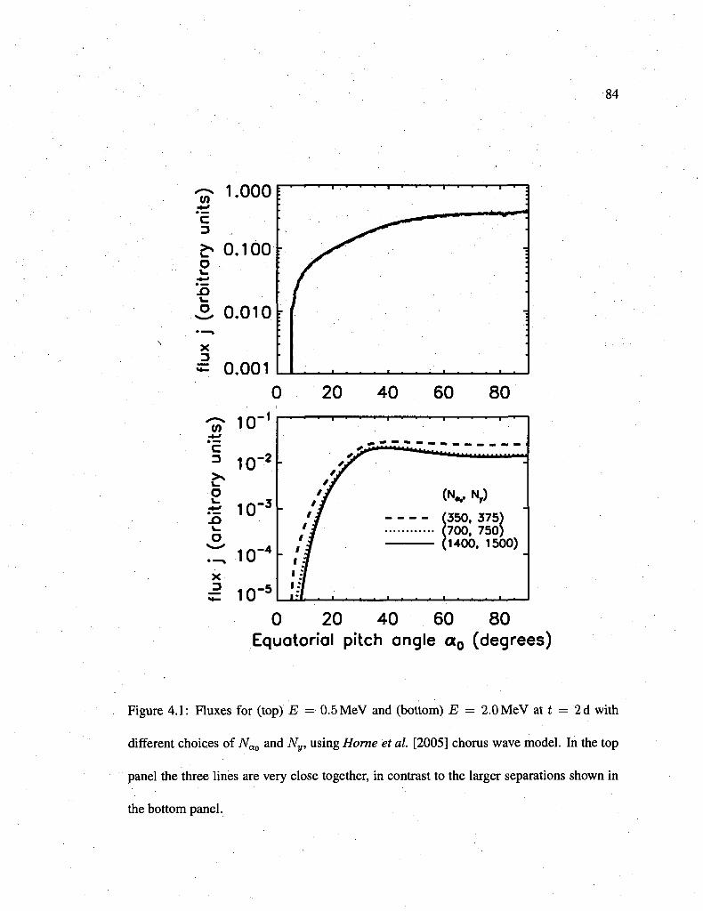
84

c 1.000

>-o.iooj o

2, 0.010

X

= 0.001

^ ^ ^ ^ • • • I ^ ^ ^ ^ ^

5 10"5

^ ^ ^ ^ ^ ^ ^ ^ ^ ^ ^ ^ ^ ^ ^ ^ ^ ^ ^ ^ ^ ^ ^ ^ _ ^

20 40 60 80

(350, 375) 700, 750) 1400, 1500)

i L i l — I — L ^ v r f M B ^ H i — J - V i — < — L - h v ^ -

0 20 40 60 80 Equatorial pitch angle a0 (degrees)

Figure 4.1: Fluxes for (top) £ = 0.5MeV and (bottom) E = 2.0MeV at t = '2d with

different choices of JVQo and JV„, using Home et al. [2005] chorus wave model. In the top

panel the three lines are very close together, in contrast to the larger separations shown in

the bottom panel.

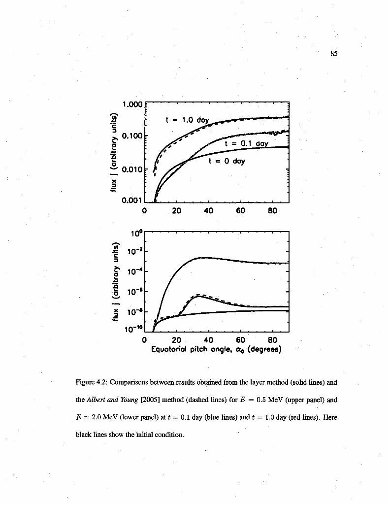
85

1 o

1.000

0.100

w 0.010 fc-

X 3

0.001

' * • ! ' I '

t - 1.0 doy f P « M ^ M l M M

20 40 60 80

10°

0 20 40 60 80 Equotoriol pitch ongle, a0 (degrees)

Figure 4.2: Comparisons between results obtained from the layer method (solid lines) and

the Albert and Young [2005] method (dashed lines) for E = 0.5 MeV (upper panel) and

E = 2.0 MeV (lower panel) at t = 0.1 day (blue lines) and t = 1.0 day (red lines). Here

black lines show the initial condition.

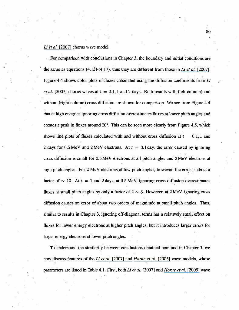
86

Li et al. [2007] chorus wave model.

For comparison with conclusions in Chapter 3, the boundary and initial conditions are

the same as equations (4.13)-(4.17), thus they are different from those in Li et al. [2007].

Figure 4.4 shows color plots of fluxes calculated using the diffusion coefficients from Li

et al. [2007] chorus waves at t = 0.1,1 and 2 days. Both results with (left column) and

without (right column) cross diffusion are shown for comparison. We see from Figure 4.4

that at high energies ignoring cross diffusion overestimates fluxes at lower pitch angles and

creates a peak in fluxes around 20°. This can be seen more clearly from Figure 4.5, which

shows line plots of fluxes calculated with and without cross diffusion at t = 0.1,1 and

2 days for 0.5 MeV and 2MeV electrons. At t = 0.1 day, the error caused by ignoring

cross diffusion is small for 0.5 MeV electrons at all pitch angles and 2 MeV electrons at

high pitch angles. For 2 MeV electrons at low pitch angles, however, the error is about a

factor of ~ 10. At t = 1 and 2 days, at 0.5 MeV, ignoring cross diffusion overestimates

fluxes at small pitch angles by only a factor of 2 ~ 3. However, at 2 MeV, ignoring cross

diffusion causes an error of about two orders of magnitude at small pitch angles. Thus,

similar to results in Chapter 3, ignoring off-diagonal terms has a relatively small effect on

fluxes for lower energy electrons at higher pitch angles, but it introduces larger errors for

larger energy electrons at lower pitch angles.

To understand the similarity between conclusions obtained here and in Chapter 3, we

now discuss features of the Li et al. [2007] and Home et al. [2005] wave models, whose

parameters are listed in Table 4.1. First, both Li et al. [2007] and Home et al. [2005] wave

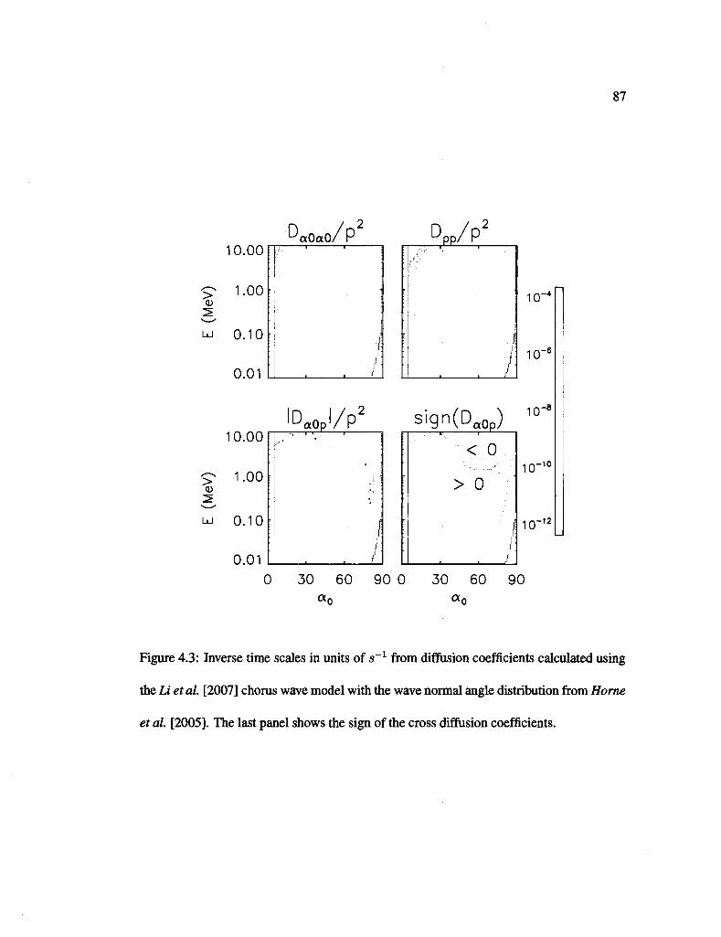
87

10.00 DaOaO/P

(MeV

)

UJ

10.00

1.00

0.10

0.01

ID

i

?.°p l/p2

:

! t '

I

. /

D£E./P2

s'gn(Dgop)

10'

10"

10"

n

•10

- 1 2

0 30 60 90 0 30 60 90

a r Oir

Figure 4.3: Inverse time scales in units of s_1 from diffusion coefficients calculated using

the Li et al. [2007] chorus wave model with the wave normal angle distribution from Home

et al. [2005]. The last panel shows the sign of the cross diffusion coefficients.

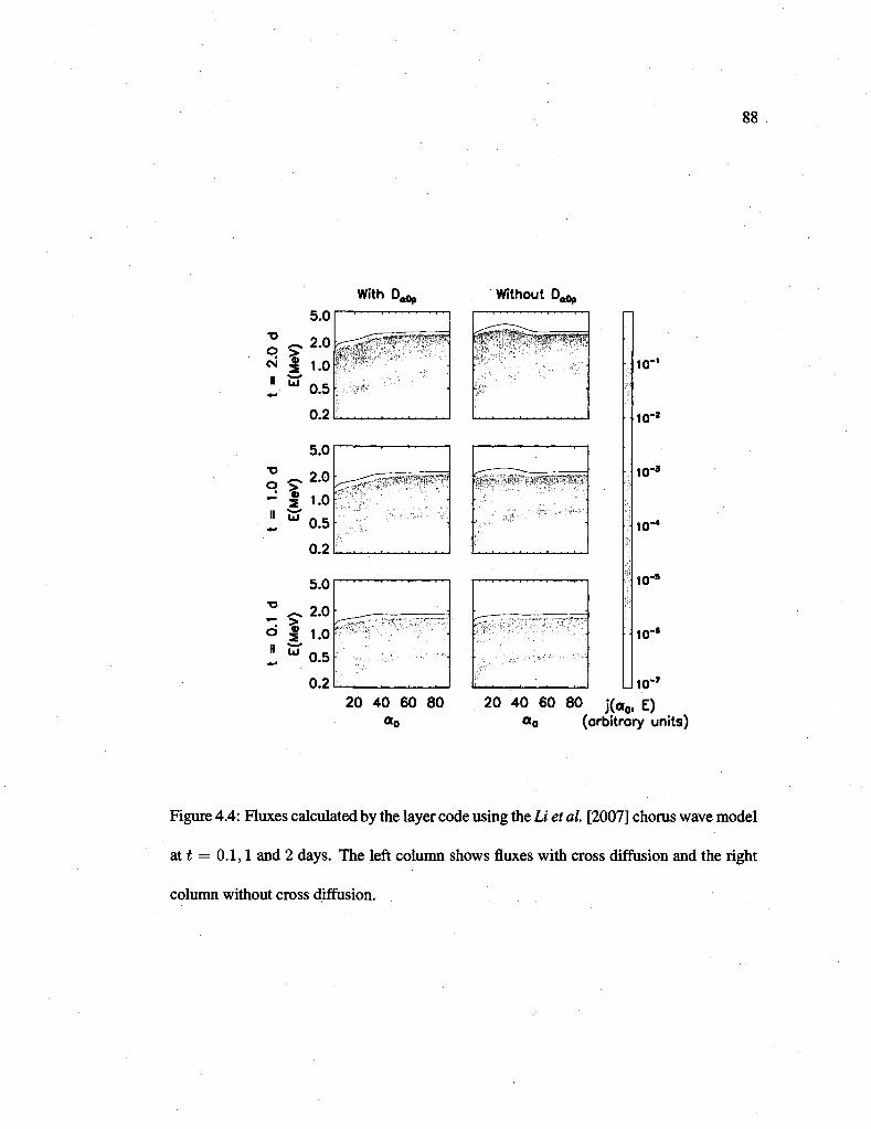
88

5.0

« - 2 . 0

II LU _ _

_ 0.5

0.2

« i in v^ Without 0,

0 | 1.0

1 " 0 . 5

10"

10"

io-

10"

10"

10"

10"

20 40 60 80 «o

20 40 60 80 j(0 o , E) «o (orbitrory units)

Figure 4.4: Fluxes calculated by the layer code using the Li et al. [2007] chorus wave model

at t = 0.1,1 and 2 days. The left column shows fluxes with cross diffusion and the right

column without cross diffusion.

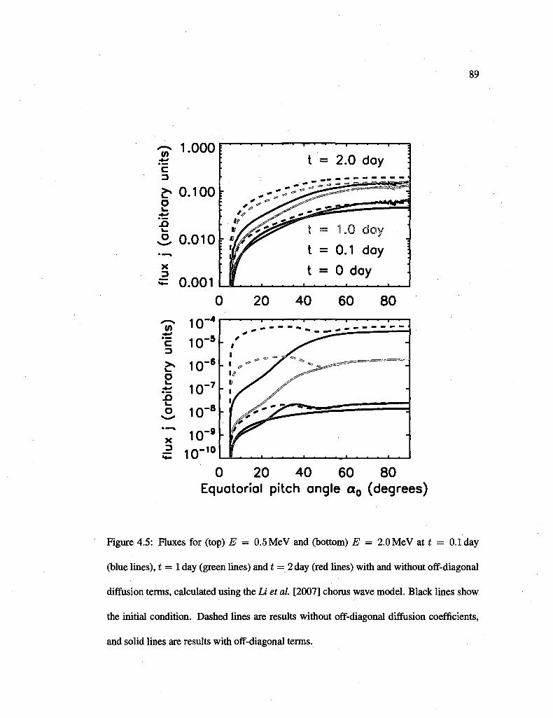
89

1.0001 r (0 +->

c ^ 0.100: o l_

•*•>

A

i l 0.010

t = 2.0 day

20 40 60 80

(0

c

^

o k.

to o

X 3 5 10

- 1 0

0 20 40 60 80 Equatorial pitch angle a 0 (degrees)

Figure 4.5: Fluxes for (top) E = 0.5 MeV and (bottom) E = 2.0 MeV at t = 0.1 day

(blue lines), t = 1 day (green lines) and t = 2 day (red lines) with and without off-diagonal

diffusion terms, calculated using the Li et al. [2007] chorus wave model. Black lines show

the initial condition. Dashed lines are results without off-diagonal diffusion coefficients,

and solid lines are results with off-diagonal terms.

90

models have similar latitudinal cutoffs of chorus wave power. For Liet al. [2007]: |A| < 35°

on the dayside, and |A| < 15° on the nightside, for Home et al. [2005]: 15° < |A| < 35° in

the prenoon sector, 10° < |A| < 35° for the afternoon sector, and |A| < 15° onthe nightside.

We see larger errors at smaller pitch angles with both models. Second, even though the Li

et al. [2007] chorus wave model has a dayside wave power increasing with latitude, which

gives a more abrupt cutoff at the maximum latitude than the Home et al. [2005] wave

model, the actual values of the wave amplitude are not very different. At A = 0°, the drift-

averaged wave amplitude for the Li et al. [2007] wave model is 6/24 x 5.6 pT + 6/24 x

50 pT = 13.9 pT, while the Home et al. [2005] model gives 7/24 x 50 pT = 14.6 pT.

At A = 35°, the drift-averaged wave amplitude for the Li et al. [2007] model in main

phase is 6/24 x 141.25 pT + 6/24 x 50 pT = 47.8 pT, while the Home et al. [2005] model

gives 6/24 x 100 pT + 3/24 x 50 pT = 31.25 pT. Thus we see that both models assume

zero amplitude above 35° latitude and have comparable wave power levels, so it is not too

surprising to see similar conclusions on ignoring cross diffusion from the two wave models.

4.3.3 Evolution of electron fluxes using a model of fast magnetosonic

waves and hiss

Interactions with fast magnetosonic waves have been recently suggested by Home et al.

[2007] to be a possible important acceleration mechanism. Because these interactions typ­

ically only involve the Landau resonance (n = 0), coupling of diffusion in a0 and p is

expected to be especially important for them. For the wave model given by Home et al.

91

[2007], the quasi-linear diffusion coefficients of the magnetosonic waves are non-zero only

over a limited range of pitch angle and energy [see Figure 9, Albert, 2008]. Thus we com­

bine the magnetosonic wave model of Home et al. [2007] outside the plasmasphere with

the main phase hiss wave model in plumes from Li et al. [2007].

The MLT averaged diffusion coefficients from magnetosonic waves (60%) and hiss

waves (15%) are shown in Figure 4.6. A similar numerical experiment as Figure 4.1 is used

to determine that Nao = 1400 and Ny = 1500 is necessary to obtain accurate solutions.

The resulting evolution of electron fluxes are plotted in Figure 4.7 at t = 0.1,1 and 2 day.

We see from the left column (results with DaoP) that the magnetosonic waves can accelerate

electrons to MeV on timescales of a day, and the fluxes show a peak around 55°, producing

a butterfly distribution, at high energies. Comparing the left column with the right column

(results without DaoP), we see that ignoring cross diffusion overestimates fluxes at larger

energies and larger pitch angles (> 55°), which is different from the effects using the

Home et al. [2005] and Li et al. [2007] chorus wave models. The effects of ignoring cross

diffusion can be seen more clearly in Figure 4.8, which shows fluxes versus equatorial pitch

angle at t = 0.1,1 and 2 days for 0.5 and 2 MeV. We see that for 0.5 MeV electrons, effects

of ignoring cross diffusion are small at all pitch angles. However, for 2 MeV electrons,

ignoring cross diffusion overestimates fluxes at large pitch angles (> 55°) by a factor of

5 ~ 10 at all three times, and by a factor of ~ 5 at small pitch angles at t = 1 and 2 days.

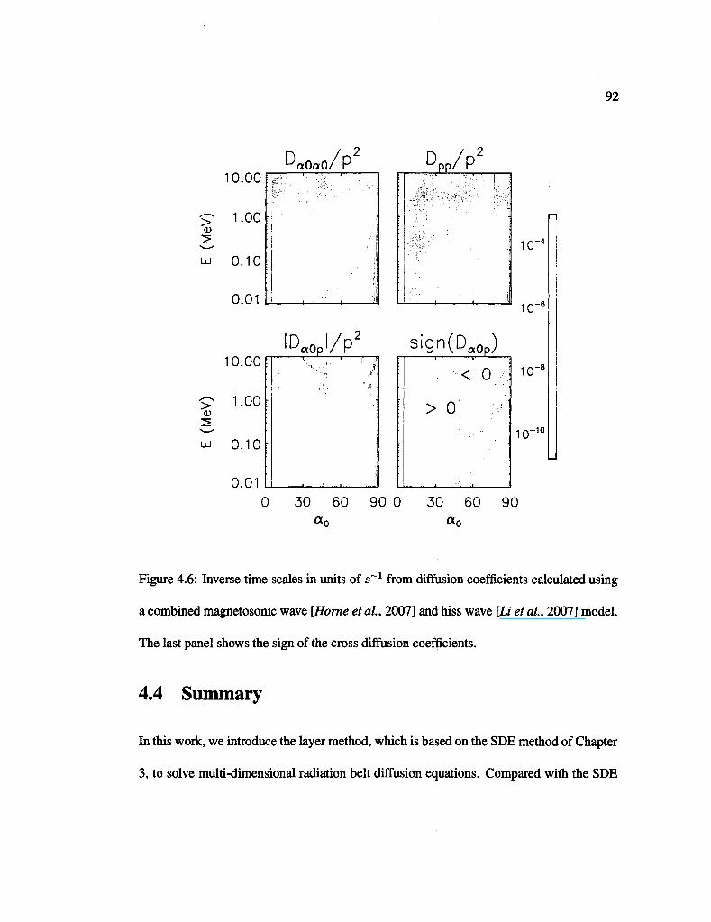
92

>

10.00

1.00

UJ 0.10

0.01

>

UJ 0.10

Da0«0/P : y p 2

10 - 4

10 - 6

iDcxOp'/p2 sign(Da0p)

0 30 60 90 0 30 60 90 Oir CLr

Figure 4.6: Inverse time scales in units of s - 1 from diffusion coefficients calculated using

a combined magnetosonic wave [Home et al, 2007] and hiss wave [Li et al, 2007] model.

The last panel shows the sign of the cross diffusion coefficients.

4.4 Summary

In this work, we introduce the layer method, which is based on the SDE method of Chapter

3, to solve multi-dimensional radiation belt diffusion equations. Compared with the SDE

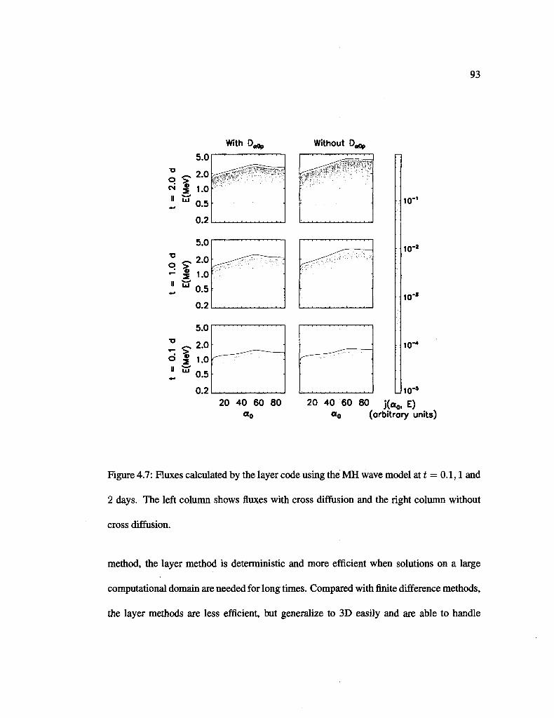
93

20 40 60 80 20 40 60 80 j(o0, E) «o «o (arbitrary units)

Figure 4.7: Fluxes calculated by the layer code using the MH wave model at t — 0.1,1 and

2 days. The left column shows fluxes with cross diffusion and the right column without

cross diffusion.

method, the layer method is deterministic and more efficient when solutions on a large

computational domain are needed for long times. Compared with finite difference methods,

the layer methods are less efficient, but generalize to 3D easily and are able to handle

94

complicated boundary geometries. We apply the layer method to a bounce-averaged pitch-

angle and energy diffusion equation and obtain excellent agreement with a previous method

[Albert and Young, 2005] using the Home et al. [2005] chorus wave model. We show that

our layer code is able to solve multi-dimensional diffusion equations with cross terms.

We then use the layer code to evaluate effects of ignoring cross diffusion using the Li

et al. [2007] chorus wave model, as a comparison with the Home et al. [2005] chorus wave

model used in Chapter 3. The main conclusion is similar to Chapter 3; i.e., ignoring off-

diagonal terms produces larger errors at smaller pitch angles and higher energies. We show

in section 4.3.2 that this similarity might be due to the fact that both wave models have a

latitudinal cutoff at 35° and comparable wave power levels.

In section 4.3.3, we show evolution of electron fluxes using a combined magnetosonic

wave [Home et al, 2005] and hiss wave model [Li et al, 2007]. We show that, despite pitch

angle scattering by hiss waves, electrons are energized to MeV in 2 days of simulation.

Ignoring cross diffusion overestimates fluxes at larger pitch angles and higher energies, in

contrast to the effects of ignoring cross diffusion using the Home et al. [2005] and Li etal

[2007] chorus wave models. Overall, we conclude that cross diffusion terms are important

and should be included when modeling diffusion of electrons in the outer radiation belt.

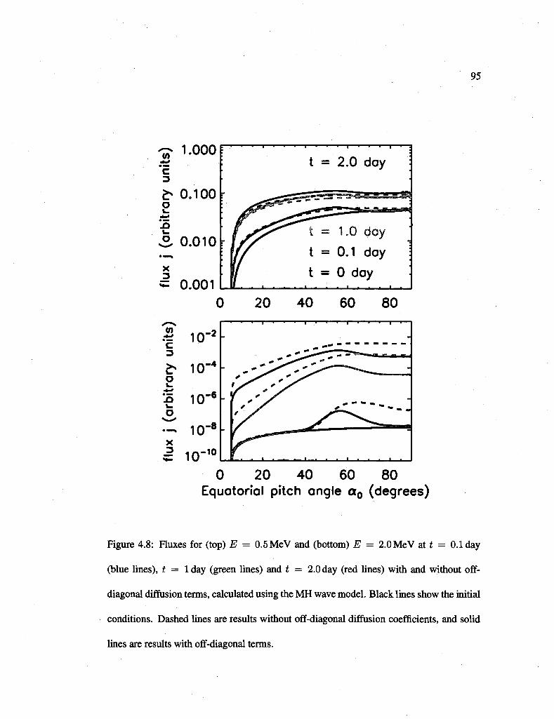
95

~ 1.000 -fr~f

c 3

>* 0.100 o

. ^ .O

sS 0.010 fe-

X

= 0.001 20 40 60 80

^ 10"10

0 20 40 60 80 Equatorial pitch angle a0 (degrees)

Figure 4.8: Fluxes for (top) E = 0.5 MeV and (bottom) E = 2.0 MeV at t = 0.1 day

(blue lines), t = lday (green lines) and t = 2.0 day (red lines) with and without off-

diagonal diffusion terms, calculated using the MH wave model. Black lines show the initial

conditions. Dashed lines are results without off-diagonal diffusion coefficients, and solid

lines are results with off-diagonal terms.

Chapter 5

Summary and future work

5.1 Summary

This thesis presents research work on a basic theory and numerical methods of modeling

of radiation belt dynamics. With the background information and review of previous work

given in Chapter 1, the main results of the thesis can be summarized as follows.

In Chapter 2 we developed a non-canonical Hamiltonian theory of relativistic charged

particles moving in slowly-varying electromagnetic fields using Lie transform analysis.

The guiding-center Lagrangian was obtained from the full Lagrangian using a Lie trans­

form, and the guiding-center equations of motion were then derived. A second Lie trans­

form was used to remove the bounce-phase dependence from the guiding-center Lagrangian

to obtain the bounce-center motion and the first-order correction to the second adiabatic in­

variant. The drift-center equations of motion and the first-order correction to the third

96

97

invariant was obtained by a third Lie transform from the bounce-center Lagrangian. Be­

cause of the use of Hamiltonian theory, the resulting equations of motion have conservation

properties which are useful for checking numerical accuracy. This work represents the first

fully Hamiltonian and relativistic theory of all three adiabatic invariants and it provides a

basis for developing theory of interactions between charged particles and waves.

Stochastic modeling of radiation belt dynamics, which results from violation of one

or more of the three adiabatic invariants, was studied in Chapter 3. We showed the SDE

method to solve diffusion equations and obtained excellent agreement between our 2D

SDE code and Albert and Young [2005] results. We then used the SDE code to explore

effects of ignoring cross diffusion and oblique waves using the Home et ah [2005] chorus

wave model. We showed that both simplifications lead to large errors of fluxes for 2 MeV

electrons at small pitch angles.

In Chapter 4, we presented the layer method, which is based on the SDE method, to

solve multi-dimensional diffusion equations. The layer method is deterministic and more

efficient than the SDE method when solutions on large number of grid points are needed for

long times. Using the layer method, we further explored effects of ignoring cross diffusion

using a Li et ah [2007] chorus wave model and a combined magnetosonic [Home et ah,

2007] and hiss [Li et ah, 2007] wave model. We showed that for the chorus wave model,

cross diffusion is more important at smaller pitch angles and higher energies, while for the

MH wave model, the cross diffusion is more important at higher pitch angles and higher

energies. We concluded from both Chapter 3 and 4 that cross diffusion can be important

and should be included to increase model accuracy.

98

5.2 Discussion and future work

This thesis has focused on time-dependent 2D modeling of quasi-linear diffusion in radi­

ation belts. The first extension would be to go from 2D to 3D, with cross diffusion terms

included. Varotsou et al. [2005] and Varotsou et al. [2008] have presented results from 3D

modeling where radial diffusion is added to a bounce-averaged pitch angle and momentum

(or energy) diffusion equation and the resulting 3D diffusion equation is solved without any

cross diffusion. We have shown in this thesis that the off-diagonal term DaoP is important

in 2D; we expect it to be also important in 3D.

To incorporate off-diagonal terms in 3D modeling, the first question is which numerical

method to use. Compared with finite difference methods, common advantages of the SDE

and layer methods are that they do not generate negative phase space densities, they can

handle different boundary geometry, and they are easy to code and generalize to 3D. The

SDE method is very efficient when solutions on a small number of grid points are needed,

especially in high dimensions. This property makes the SDE method very efficient to

calculate phase space densities along trajectories of spacecraft. Also the SDE method has

a parallelization efficiency close to 1. The layer method, on the other hand, is deterministic

and much faster than the SDE method when solutions on many phase space points are

needed. However, the layer method is still less efficient compared with finite difference

methods due to the use of large number of grid points needed to reduce numerical error.

99

The main disadvantage of standard finite difference methods, shown by Albert [2009],

is that they might produce negative phase space densities. However, it might still be helpful

to revisit finite difference methods to examine the region of negative phase space densities.

Specifically, if the region of negative phase space densities is limited to areas where phase

space densities are close to zero, and it is expected that solutions at other areas are accu­

rate because the methods are probably convergent (meaning they are stable and result in

numerical solutions that approach the analytic solution in limit At —> 0), then using finite

difference methods might be useful.

Implementation of a numerical method requires a choice of phase space coordinates.

Current 3D modeling is done in (ao, E, L) coordinates by superposing radial diffusion to a

bounce averaged pitch angle and energy diffusion equation [Shprits et ah, 2008b]. The 3D

diffusion equation is solved by an operator splitting method in three steps because the radial

diffusion part assumes constant (//, J) instead of constant (a0, E): First, the 2D bounce-

averaged pitch-angle and energy diffusion equation is stepped in time in the (a0, E) coor­

dinates. Secondly, the new (a0, E) coordinates are transformed to (//, J) space. Thirdly,

the L coordinate is stepped in time at constant (n, J), which are then transformed back

to (ao, E) space. This approach is complicated because of the coordinate transformation

and because the interpolations used during the transformation introduce more numerical

errors. Also it has been suggested recently that in an asymmetric magnetic field, a0 might

be dependent on local time itself and thus is not a suitable coordinate [Jay Albert, personal

communication, 2009].

100

Another approach to 3D modeling is to start from first principles and derive the three-

dimensional diffusion in three adiabatic invariants (/i, J, L). This approach has been taken

by Brizardand Chan [2004] using (/j,E,L) coordinates for symmetric fields. Extension

from Brizard and Chan [2004] to asymmetric fields might give us expressions of D^L and

DJL. In an asymmetric magnetic field, violation of ji or J adiabatic invariant could cause

change of particle's L value, because of drift-shell splitting [Schulz and Lanzerotti, 1974].

Thus, including D^L and DJL in the calculation might be important to reduce radiation

belt modeling error. Although there are advantages to use (//, J, L) coordinates, there are

also some difficulties. There are no codes available to evaluate diffusion coefficients of the

sort derived by Brizard and Chan [2004]. Also, boundary conditions are usually specified

on straight lines in (a0,E) space, and a straight line in (a0,E) space would become a

curve in (/j, J) space. Thus it might be harder to handle boundary conditions if using

(jj,., J, L) coordinates. Further research is needed to better understand the advantages and

disadvantages of different choices of phase-space coordinates.

To increase our model's accuracy, better wave models and initial and boundary con­

ditions are needed. For example, our calculations of diffusion coefficients D depend on

the wave models we specified; comparing Figures 4.4 and 4.7, it is easy to see that er­

rors could be large if inaccurate wave models are used. Further work should be done with

improved wave models as they become available. Also, effects of different initial condi­

tions and boundary conditions, such as relativistic kappa-type functions [Xiao et ah, 2008],

should be considered. Using available ring current codes (e.g., the Rice Convection Model

101

[Toffoletto et al, 2003]) to provide dynamic low energy boundary conditions would make

radiation belt diffusion codes more realistic.

The quasi-linear theory was developed to describe interactions between electrons and

small-amplitude broadband waves. Specifying the parameter range (e.g., wave amplitude

and/or frequency spectrum) for validity of quasi-linear theory is important. Nonlinear in­

teractions between electrons and large amplitude or narrow band waves are under intense

research, e.g., Bell [1984]; Albert [1993, 2000, 2002]; Bortnik et al. [2008] and Fumy a

et al. [2008]. Assessing the importance of nonlinear interactions and possibly including

them in radiation belt modeling are important future work.

The relativistic Hamiltonian adiabatic theory developed in this thesis is helpful to un­

derstanding the theoretical basis of radiation belt modeling. The SDE and layer methods

presented are promising in building 3D global radiation belt diffusion models. With more

advanced plasma wave models, improved initial and boundary conditions and a 3D dif­

fusion code, it is possible to build a 3D global radiation belt model whose output can be

compared with observations from upcoming spacecraft missions. The next several years

are likely to be continue to be an exciting and active period in radiation belt research.

Appendix A

Time-forward SDE method

Gardiner [1985] shows that the Fokker-Planck diffusion equation

i=l »J=1 J

corresponds to a system of stochastic differential equations

dX = b(t,x)dt + ardW(t), (A.2)

where <T<TT = a. The SDEs describe changes of x with time, and they can be used to

solve the Fokker-Planck diffusion equation (A.l) as described in Chapter 3; we call the

method "the time-forward" SDE method. To use the time-forward SDE method to solve

the bounce-averaged pitch-angle and energy diffusion equation (3.10), we first set F = Gf

and write the diffusion equation in the following form

dF d* (Daoao\+2 a2 (Daop

dt BOQ \ p2 J da0dp \ p

+ &D-F>-£i<KF)-§i»f), (A3). 102

103

where bao and bp are defined in equations (3.16) and (3.17). Thus the time-forward stochas­

tic differential equations corresponding to equation (A-3) are [Alanko-Huotari etal, 2007;

Yamada et al, 1998; Qin et al, 2005]

dA0(t) = bao(t,Ao,P)dt + andW1 + a12dW2, (A.4)

dP(t) = bp(t,A0,P)dt + a21dW1 + a22dW2, (A.5)

Where the components of the matrix er are also defined by equations (3.21) to (3.23).

Equations (A.4) and (A.5) are solved to give changes of particle coordinates (a0,p)

using the Euler-Maruyarria method [Kloeden and Platen, 1992]; i.e.,

Ao(tn+i) = A0(tn) + bao[tn,A0(tn),P{tn)]At

+ a11{tn)AW1 + ou{tn)AW2\ (A.6)

P(tn+1) = P{tn) + bp[tn,A0(tn),P(tn)}At

+ a21(tn)AW1 + a22(tn)AW2. (A.7)

After a given time period, the distribution of electrons can be obtained.

In Figure A.l, to illustrate the local effects of off-diagonal diffusion coefficients on

distributions of particles, we released 9000 particles from a0 = 30°, E = 1 MeV, where

DaoP is positive, and a0 = 50°, E = 3 MeV, where DaoP is negative (see Figure 3.1). We

chose time periods short enough to ignore boundary effects. The distribution of particles

shown in Figure A.l was obtained after t = 0.06 day for E = 3 MeV and t = 0.01 day

for E — 1 MeV. We also turned off-diagonal diffusion coefficients on and off to show local

effects of ignoring off-diagonal terms. The left panel has DaoP ^ 0, and the right panel has

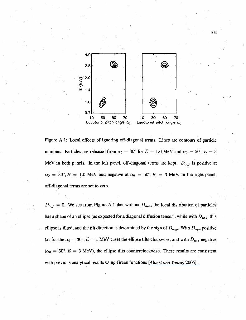
104

4.0

2.8

5* 2.0 u

w 1.4

1.0

0.7 10 30 50 70 10 30 50 70

Equatorial pitch angle a0 Equatorial pitch angle a0

Figure A.l: Local effects of ignoring off-diagonal terms. Lines are contours of particle

numbers. Particles are released from a0 = 30° for E = 1.0 MeV and a0 = 50°, E = 3

MeV in both panels. In the left panel, off-diagonal terms are kept. DaoP is positive at

a0 = 30°, E = 1.0 MeV and negative at a0 = 50°, E = 3 MeV. In the right panel,

off-diagonal terms are set to zero.

DaoP = 0. We see from Figure A.l that without Daop, the local distribution of particles

has a shape of an ellipse (as expected for a diagonal diffusion tensor), while with Daop, this

ellipse is tilted, and the tilt direction is determined by the sign of DaoP. With DaoP positive

(as for the a0 = 30°, E = 1 MeV case) the ellipse tilts clockwise, and with Daop negative

(a0 = 50°, E = 3 MeV), the ellipse tilts counterclockwise. These results are consistent

with previous analytical results using Green functions [Albert and Young, 2005].

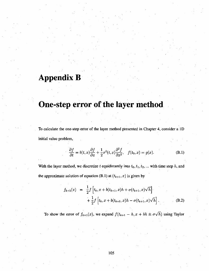
Appendix B

One-step error of the layer method

To calculate the one-step error of the layer method presented in Chapter 4, consider a ID

initial value problem,

%=6(i' x)iL+r2(i' x)% f{t°>x)=g{x)- (B.l)

With the layer method, we discretize t equidistantly into to, h, t2,... with time step h, and

the approximate solution of equation (B.l) at (ifc+i, %) is given by

fk+i(x) = « / tk,x + b(tk+i,x)h + a(tk+i,x)y/h

+ 2 / tk,x + b(tk+1,x)h-a(tk+i,x)Vh (B.2)

To show the error of fk+i(x), we expand /(ijt+i — h,x + bh ± a\fh) using Taylor

105

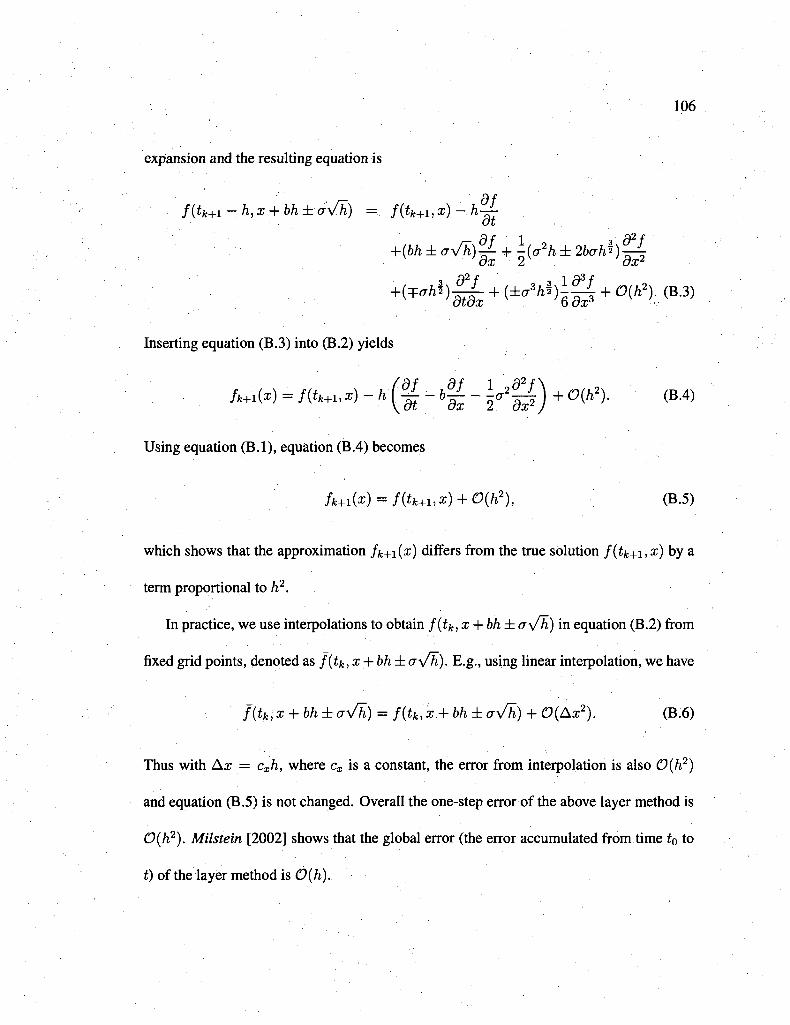
106

expansion and the resulting equation is

f(tk+i-h,x + bh±ay/h) =.. f(tk+i,x)-h—

Hbh±a^)^\{a2h±2bahi)^l

Inserting equation (B.3) into (B.2) yields

fM(x) = f(tk+1,x)-h(^L _ 6 g _ ^ 2 0 ^ + ^ 2 ) (B4)

Using equation (B.l), equation (B.4) becomes

fk+1(x) = f(tk+1,x) + 0(h2), (B.5)

which shows that the approximation fk+\{x) differs from the true solution f(tk+i,x) by a

term proportional to h2.

In practice, we use interpolations to obtain f(tk,x + bh± ay/h) in equation (B.2) from

fixed grid points, denoted as f(tk, x + bh± ay/h). E.g., using linear interpolation, we have

f(tk,x + bh±a\/h) = f(tk,x + bh±a\/h) + 0(Ax2). (B.6)

Thus with Ax = cxh, where cx is a constant, the error from interpolation is also 0(h2)

and equation (B.5) is not changed. Overall the one-step error of the above layer method is

0(h2). Milstein [2002] shows that the global error (the error accumulated from time t0 to

t) of the layer method is 0(h).

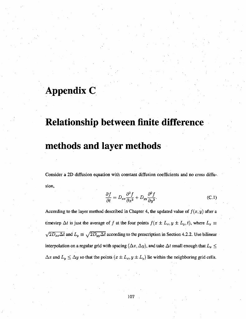
Appendix C

Relationship between finite difference

methods and layer methods

Consider a 2D diffusion equation with constant diffusion coefficients and no cross diffu­

sion,

-L = n L 4. n L (r 1 dt "dx2 wdy2' { \

According to the layer method described in Chapter 4, the updated value of f(x,y) after a

timestep At is just the average of / at the four points f(x ± Lx,y ± Ly,t), where Lx =

y/2Dxx£d and Ly = y/2Dy~y~Kt according to the prescription in Section 4.2.2. Use bilinear

interpolation on a regular grid with spacing (Ax, Ay), and take At small enough that Lx <

Ax and Ly < Ay so that the points (x ± Lx, y ± Ly) lie within the neighboring grid cells.

107

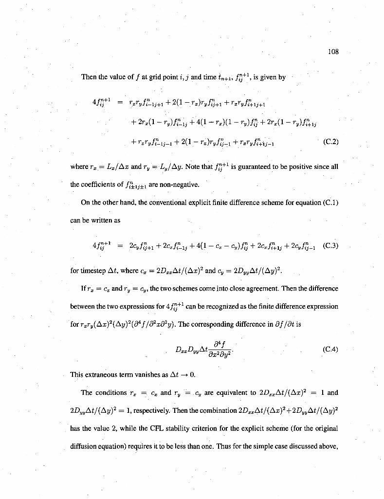
108

Then the value of / at grid point i, j and time tn+1, f%+1, is given by

4/ij = rxrvfi-lj+l + 2(1 — 7"i)r2//ij+l + rxfyfi+lj+\

+ 2rx(l-ry)f^lj + A(l-rx)(l-ry)fi; + 2rx(l-ry)f^lj

+ rxryfllj_l + 2{l-rx)ry^_l + rxrvf^lj_l (C.2)

where rx = Lx/Ax and r^ = Ly/Ay. Note that /j""1"1 is guaranteed to be positive since all

the coefficients of/^.lj±1 are non-negative.

On the other hand, the conventional explicit finite difference scheme for equation (C. 1)

can be written as

4/£+1 = 2cy/3+1 + 2pB/jB_y + 4( l -p B -c l , ) /5 + 2QB/^y + 2ci,/5_1 (C.3)

for timestep At, where cx = 2DxxAt/(Ax)2 and cy = 2DyyAt/(Ay)2.

If rx = cx and ry = Cy, the two schemes come into close agreement. Then the difference

between the two expressions for 4/,"+1 can be recognized as the finite difference expression

for rxry(Ax)2(Ay)2(d4f/d2xd2y). The corresponding difference in df/dt is

D~D»AtM?- (C4)

This extraneous term vanishes as At —> 0.

The conditions rx = cx and ry — Cy are equivalent to 2DxxAt/(Ax)2 = 1 and

2DyyAt/(Ay)2 = 1, respectively. Then the combination 2DxxAt/(Ax)2 + 2DyyAt/(Ay)2

has the value 2, while the CFL stability criterion for the explicit scheme (for the original

diffusion equation) requires it to be less than one. Thus for the simple case discussed above,

109

the layer method may be interpreted as an explicit scheme run at an unstably large timestep,

but stabilized by the small extra term ofO(At), which is the same order as the error of both

methods. This is analogous to grid diffusivity terms added to finite difference schemes in

the Lax method.

Bibliography

Abel, B., and R. M. Thome, Electron scattering loss in earth's inner magnetosphere 1.

Dominant physical processes, J. Geophys. Res., 103(A2), 2385-2396, 1998a.

Abel, B., and R. M. Thorne, Electron scattering loss in earth's inner magnetosphere 2.

Sensitivity to model parameters, J. Geophys. Res.,103(A2), 2397-2407, 1998b.

Alanko-Huotari, K., I. G. Usoskin, K. Mursula, and G. A. Kovaltsov, Stochastic simulation

of cosmic ray modulation including a wavy heliospheric current sheet, J. Geophys. Res.,

112, A08101, doi: 10.1029/2007JA012280, 2007.

Albert, J. M., Cyclotron resonance in an inhomogeneous magnetic field, Phys. Fluids B, 5,

2744, doi:10.1063/1.860715,1993.

Albert, J. M., Gyroresonant interactions of radiation belt particles with a monochromatic

electromagnetic wave, J. Geophys. Res., 105(A9), 21,191-21,209, 2000.

Albeit, J. M., Nonlinear interaction of outer zone electrons with VLF waves, Geophys. Res.

Lett., 29(8), 1275, doi:10.1029/2001GL013941, 2002.

110

I l l

Albert, J. M., Evaluation of quasi-linear diffusion coefficients for EMIC waves in a multi-

species plasma, J. Geophys. Res., 108(A6), doi:10.1029/2002JA009792, 2003.

Albert, J. M., Using quasi-linear diffusion to model acceleration and loss from wave-

particle interactions, Space Weather, 2, S09S03, doi:10.1029/2004SW000069, 2004.

Albert, J. M., Evaluation of quasi-linear diffusion coefficients for whistler mode waves

in a plasma with arbitrary density ratio, J. Geophys. Res., 110, A03218, doi:10.1029/

2004JA010844, 2005.

Albert, J. M., Simple approximations of quasi-linear diffusion coefficients, /. Geophys.

Res., 112, A12202, doi:10.1029/2007JA012551, 2007.

Albert, J. M., Efficient approximations of quasi-linear diffusion coefficients in the radiation

belts,/ Geophys. Res., 113, A06208, doi:10.1029/2007JA012936, 2008.

Albert, J. M., The coupling of quasi-linear pitch angle and energy diffusion, /. Atmos. Solar

Terres. Phys., inpress, doi:doi: 10.1016/j.jastp.2008.11.014, 2009.

Albert, J. M., and S. L. Young, Multidimensional quasi-linear diffusion of radiation belt

electrons, Geophys. Res. Lett., 32, L14110, doi:10.1029/2005GL023191, 2005.

Albright, B. J., D. Winske, D. S. Lemons, W. Daughton, and M. E. Jones, Quiet direct

simulation of coulomb collisions, IEEE Transactions on Plasma Science, 3/(1), 2003.

Baker, D. N., S. Kanekal, J. B. Blake, B. Klecker, and G. Rostoker, Satellite anomalies

linked to electron increase in the magnetosphere, Eos Trans. AGU, 75(34), 401, 1994.

112

Baker, D. N., et al., Recurrent geomagnetic storms and relatiyistic electron enhancements in

the outer magnetosphere: ISTP coordinated measurements, J. Geophys. Res., 102(A1),

14,141 - 14,148, 1997.

Bell, T. R, The nonlinear gyroresonance interaction between energetic electrons and co­

herent VLF waves propagating at an arbitrary angle with respect to the Earth's magnetic

field, J. Geophys. Res., 89(A2), 905-918, 1984.

Beutier, TV, and D. Boscher, A three-dimensional analysis of the electron radiation belt by

the Salammbo code, J. Geophys. Res., 700(A8), 14,853-14,861, 1995.

Boghosian, B. M., Covariant lagrangian methods of relativistic plasma theory, Ph.D. thesis,

University of California, Davis, 1987.

Bortnik, J., R. M. Thome, and U. S. Inan, Nonlinear interaction of energetic electrons with

large amplitude chorus, Geophys. Res. Lett., 35, L21102, doi:10.1029/2008GL035500,

2008.

Bossy, M., E. Gobet, and D. Talay, Symmetrized Euler scheme for an efficient approxima­

tion of reflected diffusions, Journal of Applied Probability, 41(3), 877 - 889, 2004.

Bourdarie, S., D. Bosher, T. Beutier, J. A. Sauvaud, M. Blanc, and R. H. W. Friedel, A

physics based model of the radiation belt flux at the day timescale, in Symposium on

Environment Modelling for Space Based Applications, SP-392, pp. 159-163, ESA Pub­

lications Division, 1996.

113

Brautigam, D. H., and J. M. Albert, Radial diffusion analysis of outer radiation belt elec­

trons during the October 9, 1990, magnetic storm, /. Geophys.Res., 105(A\), 291-309, • • (

2000.

Brizard, A. J., Nonlinear gyrokinetic tokamak physics, Ph.D. thesis, Princeton University,

1990.

Brizard, A. J., Nonlinear gyrokinetic Vlasov equation for toroidally rotating axisymmetric

tokamaks, Phys. Plasmas, 2(2), 459^71, 1995.

Brizard, A. J., Nonlinear bounce-gyrocenter Hamiltonian dynamics in general magnetic

field geometry, Phys. Plasmas, 7(8), 3238-3246, 2000.

Brizard, A. J., and A. A. Chan* Nonlinear relativistic gyrokinetic Vlasov-Maxwell equa­

tions, Phys. Plasmas, 6(12), 4548^1558, 1999.

Brizard, A. J., and A. A. Chan, Relativistic bounce-averaged quasilinear diffusion equation

for low-frequency electromagnetic fluctuations, Phys. Plasmas, S( 11), 4762-4771,2001.

Brizard, A. J., and A. A. Chan, Relativistic quasilinear diffusion in axisymmetric magnetic

geometry for arbitrary-frequency electromagnetic fluctuations, Phys. Plasmas, 11(9),

4220-4229,2004.

Brizard, A. J., and T. S. Hahm, Foundations of nonlinear gyrokinetic theory, Rev. Mod.

Phys., 79, 421-468, 2007.

114

Cary, J. R., and R. G. Littlejohn, Noncanonical Hamiltonian mechanics and its application

to magnetic field line flow, Ann. Phys., 151, 1-34, 1983.

Cattell, C, et al., Discovery of very large amplitude whistler-mode waves in Earth's radia­

tion belts, Geophys. Res. Lett., 35, L01105, doi:10.1029/2007GL032009, 2008.

Chen, Y., G. D. Reeves, and R. H. W. Friedel, The energization of relativistic electrons in

the outer Van Allen radiation belt, Nature Physics, doi:doi:10.1038/nphys655, 2007.

Costantini, C., B. Pacchiarotti, and F. Sartoretto, Numerical approximation for functionals

of reflecting diffusion processes, SIAM J. Appl. Math., 58(1), 73-102,1998.

Cully, C. M., J. W. Bonnell, and R. E. Ergun, THEMIS observations of long-lived regions

of large-amplitude whistler waves in the inner magnetosphere, Geophys. Res. Lett., 35,

L17S16, doi:10.1029/2008GL033643, 2008.

Elkington, S. R.,M. K. Hudson, and A. A. Chan, Acceleration of relativistic electrons via

drift-resonant interaction with toroidal-mode Pc-5 ULF oscillations, Geophys. Res. Lett.,

26(21), 3273-3276, 1999.

Freidlin, M., Functional integration and partial differential equations,Vrinceton University

Press, 1985.

Friedel, R. H. W., G. D. Reeves, and T. Obara, Relativistic electron dynamics in the inner

magnetosphere: a review, J. Atmos. Solar Terres. Phys., 64, 265-282, 2002.

115

Furuya, N., Y. Omura, and D. Summers, Relativistic turning acceleration of radiation

belt electrons by whistler mode chorus, J. Geophys. Res., 113, A04224, doi:i0.1029/

2007JA012478, 2008.

Gardiner, C. W., Handbook of Stochastic Methods for Physics, Chemistry and the Natural

Sciences, Springer-Verlag, 1985.

Glauert, S. A., and R. B. Home, Calculation of pitch angle and energy diffusion coefficients

with the PADIE code, J. Geophys. Res., 110, A04206, doi:10.1029/2004JA010851,

2005.

Goldstein, H., Classical Mechanics, 2nd ed., Addison-Wesley, Reading, Mass., 1980.

Grebogi, C, and R. G. Littlejohn, Relativistic ponderomotive hamiltonian, Phys. Fluids,

27(8), 1996-2004, 1984.

Green, J. C, and M. G. Kivelson, Relativistic electrons in the outer radiation belt: Dif­

ferentiating between acceleration mechanisms, J. Geophys. Res., 109, A03213, doi:

10.1029/2003JA010153, 2004.

Hilmer, R. V., G. R Ginet, and T. E. Cay ton, Enhancement of equatorial energetic elec­

tron fluxes near L = 4.2 as a result of high speed solar wind streams, J. Geophys. Res.,

705(A1O), 23,311-23,322, 2000.

Home, R. B., and R. M. Thome, Potential waves for relativistic electron scattering and

116

stochastic acceleration during magnetic storms, Geophys. Res. Lett., 25(15), 3011-3014,

1998.

Home, R. B., and R. M. Thorne, Relativistic electron acceleration and precipitation during

resonant interactions with whistler-mode chorus, Geophys. Res. Lett., 30(10), 1527, doi:

10.1029/2003GL016973, 2003.

Home, R. B., S. A. Glauert, and R. M. Thome, Resonant diffusion of radiation belt

electrons by whistler-mode chorus, Geophys. Res. Lett., 30(9), 1493, doi:10.1029/

2003GL016963, 2003.

Home, R. B., R. M. Thome, S. A. Glauert, J. M. Albert, N. P. Meredith, and R. R. Ander­

son, Timescale for radiation belt electron acceleration by whistler mode chorus waves,

J. Geophys. Res., 110, A03225,doi:10.1029/2004JA010811, 2005.

Home, R. B., R. M. Thome, S. A. Glauert, N. P. Meredith, D. Pokhotelov, and O. San-

tolfk, Electron acceleration in the Van Allen radiation belts by fast magnetosonic waves,

Geophys. Res. Lett., 34, L17107, doi:10.1029/2007GL030267, 2007.

Kennel, C. F., and F. Engelmann, Velocity space diffusion from weak plasma turbulence in

a magnetic field, Phys. Fluids, 9(12), 1966.

Khazanov, G. V, and K. V. Gamayunov, Effect of oblique electromagnetic ion cy­

clotron waves on relativistic electron scattering: Combined Release and Radiation Ef-

117

fects Satellite (CRESS)-based calculation, J. Geophys. Res., 112, A07220, doi:10.1029/

2007JA012300, 2007.

Kim, H.-J., and A. A. Chan, Fully adiabatic changes in storm time relativistic electron

fluxes, J. Geophys.Res., 102(A10), 22,107-22,116, 1997.

Kivelson, M. G., and C. T. Russell (Eds.), Introduction to Space Physics, Cambridge Uni­

versity Press, 1995.

Kloeden, P. E., and E. Platen, Numerical Solution of Stochastic Differential Equations,

Springer-Verlag, 1992.

Kress, B. T., M. K. Hudson, M. D. Looper, J. M. Albert, J. G. Lyon, and C. C. Goodrich,

Global MHD test particle simulations of > 10 MeV radiation belt electrons during storm

sudden commencement, J. Geophys. Res., 112, A09215, doi:10.1029/2006JA012218,

2007.

Lam, M. M., R. B. Home, N. P. Meredith, and S. A. Glauert, Modeling the effects of radial

diffusion and plasmaspheric hiss on outer radiation belt electrons, Geophys. Res. Lett.,

34, L20112, doi:10.1029/2007GL031598, 2007.

Li, W., Y. Y. Shprits, and R. M. Thorne, Dynamic evolution of energetic outer zone elec­

trons due to wave-particle interactions during storms, J: Geophys. Res., 112, A10220,

doi:10.1029/2007JA012368, 2007.

Li, X., and M. A. Temerin, The electron radiation belt, Space Set Rev., 95, 569-580, 2001.

118

Littlejohn, R. G., Hamiltonian formulation of guiding center motion, Phys. Fluids, 24,

1730-1749,1981.

Littlejohn, R. G., Hamiltonian theory of guiding center bounce motion, Phys. Scr., T2/1,

119-125,1982.

Littlejohn, R. G., Variational principles of guiding centre motion, J. Plasma Phys., 29,

111-125,1983.

Lorentzen, K. R., J. B. Blake, U. S. Inan, and J. Bortnik, Observations of relativistic elec­

tron microbursts in association with vlf chorus, /. Geophys. Res., 106(A4), 6017-6027,

2001.

Lyons, L. R., General relations for resonant particle diffusion in pitch angle and energy,

J. Plasma Phys,, 72(45), 1974a.

Lyons, L. R., Pitch angle and energy diffusion coefficients from resonant interactions with

ion-cyclotron and whistler waves, J. Plasma Phys., 72(417), 1974b.

Lyons, L. R., and R. M. Thorne, Equilibrium structure of radiation belt electrons, J. Geo­

phys. Res., 78(13), 2142-2149,1973.

Meredith, N. P., M. Cain, R. B. Home, R. M. Thorne, D. Summers, and R. R. Ander­

son, Evidence for chorus-driven electron acceleration to relativistic energies from a

survey of geomagnetically disturbed periods, J. Geophys. Res., 108(A6), doi:10.1029/

2002JA009764, 2003a.

119

Meredith, N. P., R. B. Home, R. M. Thorne, and R. R. Anderson, Favored regions for

chorus-driven electron acceleration to relativistic energies in the Earth's outer radiation

belt, Geophys. Res. Lett, 30(16,1871), doi:10.1029/2003GL017698, 2003b.

Meredith, N. P., R. B. Home, S. A. Glauert, and R. R. Anderson, Slot region electron loss

timescales due to plasmaspheric hiss and lightning-generated whistlers, J. Geophys. Res.,

112, A08214, doi:10.1029/2007JA012413, 2007.

Milstein, G. N., The probability approach to numerical solution of nonlinear parabolic

equations, Numerical Methods for Partial Differential Equations, 18, 490-522, doi:10.

1002/num. 10020, 2002.

Milstein, G. N., and M. V. Tretyakov, Numerical solution of the Dirichlet problem for

nonlinear parabolic equations by a probabilistic approach, IMA Journal of Numerical

Analysis, 21, 887-917, 2001.

Milstein, G. N., and M. V. Tretyakov, A probabilistic approach to the solution of the neu-

mann problem for nonlinear parabolic equations, IMA Journal of Numerical Analysis,

22,599-622,2002.

Northrop, T. G., The Adiabatic Motion of Charged Particles, Wiley-Interscience Publishers,

New York, 1963.

Northrop, T. G., C. S. Liu, and M. D. Kruskal, First correction to the second adiabatic

invariant of charged-particle motion, Phys. Fluids, 9(8), 1503 - 1513,1966.

120

O'Brien, T. P., K. R. Lorentzen, I. R. Mann, N. P. Meredith, J. B. Blake, J. F. Fennell,

M. D. Looper, D. K. Milling, and R. R. Anderson, Energization of relativistic electrons

in the presence of ULF power and MeV microbursts: Evidence for dual ULF and VLF

acceleration, J. Geophys. Res., /0S(A8,1329), doi: 10.1029/2002JA009784, 2003.

O'Brien, T. P., M. D. Looper, and J. B. Blake, Quantification of relativistic electron

microburst losses during the GEM storms, Geophys. Res. Lett, 31, L04802, doi:

10.1029/2003GL018621, 2004.

Oksendal, B., Stochastic Differential Equations: An Introduction with Applications, third

ed., Springer-Verlag, 1992.

Press, W. H., S. A. Teukolsky, W. T. Vetterling, and B. P. Flannery, Numerical Recipes in

C++: The Art of Scientific Computing, second edition ed., Cambridge University Press,

2002.

Qin, G., M. Zhang, J. R. Dwyer, H. K. Rassoul, and G. M. Mason, The model dependence

of solar energetic particle mean free paths under weak scattering, Astrophys. J., 627(1),

562-566, 2005.

Reeves, G. D., K. L. McAdams, R. H. W. Friedel, and T. P. O'Brien, Acceleration and loss

of relativistic electrons during geomagnetic storms, Geophys. Res. Lett., 30(10,1529),

doi:10.1029/2002GL016513, 2003.

, " • 1 2 1

Roederer, J. G., Dynamics of Geomagnetically Trapped Radiation, Physics and Chemistry

in Space, vol. 2, Springer, Berlin, Germany; New York, U. S. A. , 1970.

Schulz, M., and L. J. Lanzerotti, Particle Diffusion in the Radiation Belts, Physics and

Chemistry in Space, vol. 7, Springer-Verlag, 1974.

Shprits, Y. Y, W. Li, and R. M. Thorne, Controlling effect of the pitch angle scattering

rates near the edge of the loss cone on electron lifetimes, J. Geophys. Res., Ill, A12206,

doi: 10.1029/2006JA011758, 2006a.

Shprits, Y. Y, R. M. Thorne, R. B. Home, S. A. Glauert, M. Cartwright, C. T. Russell,

D. N. Baker, and S. G. Kanekal, Acceleration mechanism responsible for the formation

of the new radiation belt during the 2003 Halloween solar storm, Geophys. Res. Lett,

33, L05104, doi:10.1029/2005GL024256, 2006b.

Shprits, Y Y, R. M. Thorne, R. B. Home, and D. Summers, Bounce-averaged diffusion

coefficients for field-aligned chorus waves, J. Geophys. Res., Ill, A10225, doi: 10.1029/

2006JA011725, 2006c.

Shprits, Y Y, S. R. Elkington, N. R Meredith, and D. A. Subbotin, Review of modeling

of losses and sources of relativistic electrons in the outer radiation belt I: Radial trans­

port, J. Atmos. Solar Terres.Phys., 70, 1679-1693, doi:doi:10.1016/j.jastp.2008.06.008,

2008a.

Shprits, Y Y, D. A. Subbotin, N. R Meredith, and S. R. Elkington, Review of modeling of

122

losses and sources of relativistic electrons in the outer radiation belt II: Local acceleration

and loss, /. Atmos. Solar Terres.Phys., 70,1694-1713, doi:10.1016/j.jastp.2008.06.014,

2008b.

Summers, D., Quasi-linear diffusion coefficients for field-aligned electromagnetic waves

with applications to the magnetosphere, J. Geophys. Res., 110, A08213, doi:10.1029/

2005JA011159, 2005.

Summers, D., and R. M. Thorne, Relativistic electron pitch-angle scattering by electro­

magnetic ion cyclotron waves during geomagnetic storms, /. Geophys. Res., 108(A4),

doi:10.1029/2002JA009489, 2003.

Summers, D., R. M. Thorne, and F. Xiao, Relativistic theory of wave particle resonant

diffusion with application to electron acceleration in the magnetosphere, J. Geophys.

Res., 703,20,487, 1998.

Summers, D., B. Ni, and N. P. Meredith, Timescales for radiation belt electron acceleration

and loss due to resonant wave-particle interactions: 1. Theory, J. Geophys. Res., 112,

A04206, doi:10.1029/2006JA011801, 2007a.

Summers, D., B. Ni, and N. R Meredith, Timescales for radiation belt electron acceleration

and loss due to resonant wave-particle interactions: 2. Evaluation for VLF chorus, ELF

hiss, and electromagnetic ion cyclotron waves, J. Geophys. Res., 112, A04207, doi:10.

1029/2006JA011993, 2007b.

123

Tao, X., A. A. Chan, and A. J. Brizard, Hamiltonian theory of adiabatic motion of relativis-

tic charged particles, Phys. Plasmas, 74(092107), doi: 10.1063/1.2773702, 2007.

Tao, X., A. A. Chan, J. M. Albert, and J. A. Miller, Stochastic modeling of mul­

tidimensional diffusion in the radiation belts, J. Geophys. Res., 113, A07212, doi:

10.1029/2007JA012985, 2008.

Tao, X., J. M. Albert, and A. A. Chan, Numerical modeling of multidimensional diffusion

in the radiation belts using layer methods, J. Geophys. Res., 114, A02215, doi:10.1029/

2008JA013826, 2009.

Thorne, R. M., Energetic radiation belt electron precipitation: A natural depletion mecha­

nism for stratospheric ozone, Science, 795(4275), 287 - 289, doi:10.1126/science.l95.

4275.287, 1977.

Thorne, R. M., E. J. Smith, R. K. Burton, and R. E. Holzer, Plasmaspheric hiss, J. Geophys.

Res., 78(10), 1581-1596, 1973.

Thorne, R. M, T. P. O'Brien, Y..Y. Shprits, D. Summers, and R. B. Home, Timescale

for MeV electron microburst loss during geomagnetic storms, J. Geophys. Res., 110,

A09202, doi:10.1029/2004JA010882, 2005.

Toffoletto, F...S. Sazykin, R. Spiro, and R. Wolf, Inner magnetospheric modeling with the

rice convection model, Space Sci. Rev., 107, 175-196, 2003.

124

Van Allen, J. A., and L. A. Frank, Radiation around the Earth to a radial distance of 107,400

km, Nature, 183, 430-434, doi:10.1038/183430a0, 1959.

Varotsou, A., D. Boscher, S. Bourdarie, R. B. Home, S. A. Glauert, and N. P. Meredith,

Simulation of the outer radiation belt electrons near geosynchronous orbit including both

radial diffusion and resonant interaction with whistler-mode chorus waves, Geophys.

Res. Lett., 32, L19106, doi:10.1029/2005GL023282, 2005.

Varotsou, A., D. Boscher, S. Bourdarie, R. B. Home, N. P. Meredith, S. A. Glauert, and

R. H. Friedel, Three-dimensional test simulations of the outer radiation belt electron dy­

namics including electron-chorus resonant interactions, J. Geophys. Res., 113, A12212,

doi:10.1029/2007JA012862, 2008.

Xiao, R, H. He, Q. Zhou, H. Zheng, and S. Wang, Relativistic diffusion coefficients for

superluminous (auroral kilometric radiation) wave modes in space plasmas, J. Geophys.

Res., Ill, A11201,doi:10.1029/2006JA011865, 2006.

Xiao, F., L. Chen, H. Zheng, and S. Wang, A parametric ray tracing study of superluminous

auroral kilometric radiation wave modes, J. Geophys. Res., 112, A10214, doi:10.1029/

2006JA012178, 2007.

Xiao, F., C. Shen, Y. Wang, H. Zheng, and S. Wang, Energetic electron distributions fitted

with a relativistic kappa-type function at geosynchronous orbit, J. Geophys. Res., 113,

A05203, doi:10.1029/2007JA012903, 2008.

125

Yamada, Y., S. Yanagita, and T. Yoshida, A stochastic view of the solar modulation phe­

nomena of cosmic rays, Geophys. Res. Lett., 25(13), 2353-2356, 1998.

Zhang, M., A Markov stochastic process theory of cosmic-ray modulation, Astrophys. J.,

573,409^20,1999.