h-Blossoming: A new approach to algorithms and identities for h-Bernstein bases and h-Bézier curves

Computer Aided Geometric Design 28 (2011) 549–565

Contents lists available at SciVerse ScienceDirect

Computer Aided Geometric Design

www.elsevier.com/locate/cagd

h-Blossoming: A new approach to algorithms and identities forh-Bernstein bases and h-Bézier curves ✩

Plamen Simeonov a, Vasilis Zafiris a, Ron Goldman b,∗a Department of Computer and Mathematical Sciences, University of Houston-Downtown, Houston, TX 77002, United Statesb Department of Computer Science, Rice University, Houston, TX 77251, United States

a r t i c l e i n f o a b s t r a c t

Article history:Received 31 December 2010Received in revised form 23 June 2011Accepted 21 September 2011Available online 29 September 2011

Keywords:h-Blossomh-Bernstein basish-Bézier curveMarsden’s identitySubdivision

A new variant of the blossom, the h-blossom, is introduced by altering the diagonalproperty of the standard blossom. The significance of the h-blossom is that the h-blossomsatisfies a dual functional property for h-Bézier curves over arbitrary intervals. Using theh-blossom, several new identities involving the h-Bernstein bases are developed includingan h-variant of Marsden’s identity. In addition, for each h-Bézier curve of degree n,a collection of n! new, affine invariant, recursive evaluation algorithms are derived. Usingtwo of these recursive evaluation algorithms, a recursive subdivision procedure for h-Béziercurves is constructed. Starting from the original control polygon of an h-Bézier curve, thissubdivision procedure generates a sequence of control polygons that converges rapidly tothe original h-Bézier curve.

© 2011 Elsevier B.V. All rights reserved.

1. Introduction

Blossoming is a powerful technique for analyzing the properties of Bézier and B-spline curves and surfaces. Algorithmsfor recursive evaluation, subdivision, differentiation, degree elevation, and knot insertion for Bézier and B-spline curves andsurfaces are all readily derived using blossoming (Ramshaw, 1987, 1988, 1989). The purpose of this paper is to investigatealgorithms and identities for the h-Bernstein bases and h-Bézier curves by introducing a new form of the blossom, theh-blossom, specifically adapted to analyzing h-Bernstein bases and h-Bézier curves.

The h-Bernstein basis functions

Bnk(t;h) =

(n

k

)∏k−1i=0 (t + ih)

∏n−k−1i=0 (1 − t + ih)∏n−1

i=0 (1 + ih), (1.1)

k = 0, . . . ,n, have been studied both in Approximation Theory and in Computer Aided Geometric Design. In ApproximationTheory, Stancu (1968, 1984) introduced these functions and showed that for h > 0 the operator

Bn[ f ;h](t) =n∑

k=0

f (k/n)Bnk(t;h)

shares many properties with standard Bernstein approximation (the case h = 0). Many years later, these same basis functionswere rediscovered by Goldman (1985) and Goldman and Barry (1991), who called them Pólya polynomials because they

✩ This paper has been recommended for acceptance by J. Peters.

* Corresponding author.E-mail addresses: [email protected] (P. Simeonov), [email protected] (V. Zafiris), [email protected] (R. Goldman).

0167-8396/$ – see front matter © 2011 Elsevier B.V. All rights reserved.doi:10.1016/j.cagd.2011.09.003

http://dx.doi.org/10.1016/j.cagd.2011.09.003

http://www.ScienceDirect.com/

http://www.elsevier.com/locate/cagd

mailto:[email protected]



http://dx.doi.org/10.1016/j.cagd.2011.09.003

550 P. Simeonov et al. / Computer Aided Geometric Design 28 (2011) 549–565

represent the discrete probability distribution generated by Pólya’s urn model. Soon after the work of Goldman and Barry,Neamtu (1991) and Sablonniere (1992) studied what they called discrete Bernstein polynomials, which are closely relatedto the h-Bernstein polynomials in Eq. (1.1). Neamtu was particularly interested in the relationship between these discreteBernstein polynomials and discrete simplex splines; therefore he restricted his attention to the cases where the parametert takes on only discrete values. Sablonniere studied the continuous case of polynomials P (t) over intervals [0, N], whereN � deg(P ). He reproduced many of the formulas of Goldman and Barry, and he also derived some new results on finitedifferences and subdivision for these discrete Bernstein polynomials.

Goldman and Barry showed that for h > 0 the h-Bézier curves

P (t) =n∑

k=0

Bnk(t;h)Pk, 0 � t � 1 (1.2)

(which they called Pólya curves) share many properties with standard Bézier curves (the case h = 0). They are affine in-variant, lie in the convex hull of their control points, satisfy the variation diminishing property, are non-degenerate, andreproduce linear functions. In addition, these curves possess analogous algorithms for recursive evaluation and degree ele-vation. Missing, however, from their analysis are simple algorithms for blossoming, subdivision, and differentiation. One ofthe main goals of this paper is to develop blossoming and subdivision procedures for h-Bézier curves. Differentiation algo-rithms for h-Bézier curves over arbitrary intervals along with extensions of h-Bézier curves to the h-analogues of B-splinecurves will be treated in a separate paper using the homogeneous variant of the h-blossom.

This paper makes four principal contributions:

Blossoming: We introduce a new variant of the blossom, the h-blossom, especially adapted for proving new identities forh-Bernstein bases and deriving novel algorithms for h-Bézier curves.

Identities: Using the h-blossom, we derive new identities for the h-Bernstein bases including an h-variant of Marsden’sidentity.

Recursive Evaluation Algorithms: Again invoking the h-blossom, we construct for each h-Bézier curve of degree n, a collectionof n! new, affine invariant, recursive evaluation algorithms.

Subdivision: Using two of these new recursive evaluation algorithms, we present for the first time a subdivision procedurefor h-Bézier curves over arbitrary intervals.

Thus this paper is a companion to Simeonov et al. (2010), where we introduce the q-blossom in order to derive analogousalgorithms and identities for q-Bernstein bases and q-Bézier curves (Lewanowicz and Wozny, 2004; Phillips, 1997a, 1997b,2010).

The h-Bézier curves of degree n over a fixed interval [a,b] are a 1-parameter family of curves. The parameter h is a shapeparameter: increasing h from zero moves the curve closer and closer to the straight line joining the first and the last controlpoints; decreasing h past zero pushes the curve further and further away from this line, until a series of singularities areencountered at h = −(b − a)/k, k = (n − 1), . . . ,1, after which the curve again approaches the straight line joining the firstand the last control points – see Fig. 1 and Goldman (1985). But beyond this modest effect as a simple shape parameter,we expect that these h-Bernstein bases and h-Bézier curves will be of use in CAGD for several additional reasons.

First, both Lagrange interpolation (h = −(b − a)/n) and Bézier approximation (h = 0) are special cases of h-Bézier curvesover arbitrary intervals. Thus the value of h provides a natural transition between interpolation and approximation forpolynomial curves and surfaces. Moreover, for each value of h all the standard algebraic machinery of CAGD – recursiveevaluation, subdivision, degree elevation, blossoming – is readily available, and many fundamental geometric properties –affine invariance, linear precision, interpolation of end points, non-degeneracy – are also preserved.

Second, even though Bernstein polynomials are used in CAGD as an exact representation for curves and surfaces, inpractice it is not possible to manufacture these curves and surfaces exactly as specified; manufacturing always has toleranceson what can actually be fabricated. Using h-Bernstein polynomials, we can build in such tolerances for Bézier curves andsurfaces during design by taking values of h near zero – that is, by putting a tolerance on the value of h. Once again allthe algebraic machinery of CAGD (recursive evaluation, subdivision, degree elevation, blossoming) is readily available forall values of h, and many important geometric properties (affine invariance, linear precision, interpolation at end points,non-degeneracy as well as the convex hull and variation diminishing properties when h � 0) are also preserved.

Third, h-Bézier curves play a fundamental role in the analysis of discrete B-splines, piecewise polynomials whose forwarddifferences rather than their derivatives agree at the knots. These discrete B-splines were first introduced by Mangasarianand Schumaker (1971) to study certain minimization problems involving differences. Such discrete B-splines have also beeninvestigated in Dikshit and Powar (1982), Dikshit and Rana (1987), Lyche (1975, 1976), Mangasarian and Schumaker (1971,1973), Rana (1988), Schumaker (1981). We plan to take up the study of these discrete B-splines shortly. We will show thatusing knot insertion to convert from discrete B-spline to piecewise h-Bézier form plays a central role in the analysis of thesediscrete splines.

Finally, Neamtu (1991) showed that there is a close relationship between h-Bernstein basis functions and discrete simplexsplines. Thus h-Bernstein polynomials appear in many guises both in Approximation Theory and in CAGD.

P. Simeonov et al. / Computer Aided Geometric Design 28 (2011) 549–565 551

Fig. 1. The effect of changing the h-parameter (left) and scaling the length, �, of the domain interval (right) of a cubic h-Bézier curve.

This paper is organized in the following fashion. In Section 2 we introduce the basic definitions, fundamental formulas,and explicit notation for h-Bernstein bases and h-Bézier curves over arbitrary intervals. The h-blossom is defined in Sec-tion 3, where the existence and the uniqueness of the h-blossom are also established. In Section 4 we invoke the h-blossomto develop novel recursive evaluation algorithms for h-Bézier curves, and in Section 5 we use the h-blossom to derivenew identities involving the h-Bernstein basis functions. We then apply these identities to establish several of the standardgeometric properties of h-Bézier curves. A subdivision algorithm for h-Bézier curves is developed in Section 6, where therapid convergence of the control polygons generated by repeated application of this algorithm is also demonstrated. Weclose in Section 7 with a short summary of our work, along with a brief discussion of two promising problems for futureresearch.

2. h-Bézier curves

For many applications and in particular for subdivision, we need h-Bernstein bases over arbitrary intervals. The h-Bernstein basis functions over the interval [a,b] are defined by

Bnk

(t; [a,b];h

) =(

n

k

)∏k−1i=0 (t − a + ih)

∏n−k−1i=0 (b − t + ih)∏n−1

i=0 (b − a + ih), (2.1)

k = 0, . . . ,n. To avoid zeroes in the denominator on the right-hand side of Eqs. (2.1), values of h for which b = a − jh forsome 0 � j � n − 1 are excluded.

Notice that we have the following important special cases:

1. When a = 0 and b = 1, Eq. (2.1) reduces to Eq. (1.1) for the standard h-Bernstein basis functions over the interval [0,1]studied first by Stancu and later by Goldman and Barry.

2. When h = 0, Eq. (2.1) reduces to the equation for the standard Bernstein basis functions over the interval [a,b].3. When b = a − nh, Eq. (2.1) reduces to the equation for the Lagrange basis functions of degree n for the nodes a,

a − h, . . . ,a − nh (see Section 5, Proposition 5.10 and Goldman, 2003, Section 2.5).

Notice too that these Bernstein basis functions have the following invariance properties:

Translation invariance

Bnk

(t + c; [a + c,b + c];h

) = Bnk

(t; [a,b];h

)for all c. (2.2)

Scale invariance

Bnk

(ct; [ca, cb]; ch

) = Bnk

(t; [a,b];h

)for all c �= 0. (2.3)

Translating by −a and then scaling by 1/(b − a), we find that


Fig. 2. The h-de Casteljau algorithm for a cubic h-Bézier curve on the interval [a,b].

Bnk

(t; [a,b];h

) = Bnk

(t − a

b − a; [0,1]; h

b − a

)= Bn

k

(t − a

b − a; h

b − a

). (2.4)

The h-Bernstein basis functions in Eq. (2.1) form a partition of unity (see Proposition 5.2), provide a basis for all poly-nomials of degree at most n (see Corollary 4.4), are non-negative for all h � 0 and a � t � b, and satisfy the followingrecurrence:

B00

(t; [a,b];h

) = 1,

Bnk

(t; [a,b];h

) = t − a + (k − 1)h

b − a + (n − 1)hBn−1

k−1

(t; [a,b];h

) + b − t + (n − k − 1)h

b − a + (n − 1)hBn−1

k

(t; [a,b];h

). (2.5)

The h-Bézier curve of degree n over the interval [a,b] with control points P0, . . . , Pn is the polynomial curve defined by

P (t) =n∑

i=0

Pi Bni

(t; [a,b];h

), t ∈ [a,b]. (2.6)

Warning: Scaling the length � = b − a of the parameter interval [a,b] by a constant c, but failing to also scale the parame-ter h will lead to a different h-Bézier curve – see Eqs. (2.3) and (2.6). This effect is illustrated in Fig. 1, right.

The standard geometric properties of h-Bézier curves – affine invariance, convex hull, variation diminishing – can bederived from the comparable algebraic properties – partition of unity, non-negativity, Descartes Law of Signs – of theh-Bernstein basis functions – see Section 5. The following h-de Casteljau evaluation algorithm is a direct consequence of therecurrence Eq. (2.5) for the h-Bernstein basis functions.

The h-de Casteljau evaluation algorithm For k = 0, . . . ,n, set P 0k (t) = Pk . For r = 1, . . . ,n and k = 0, . . . ,n − r set:

P rk(t) = b − t + (n − r − k)h

b − a + (n − r)hP r−1

k (t) + t − a + kh

b − a + (n − r)hP r−1

k+1(t). (2.7)

Then P (t) = Pn0(t) is the point on the h-Bézier curve with parameter value t ∈ [a,b].

Notice that this recursive evaluation algorithm reduces to the standard de Casteljau evaluation algorithm for Béziercurves when h = 0, and reduces to Neville’s evaluation algorithm for Lagrange interpolation when b = a − nh (Goldman,2003).

The h-de Casteljau algorithm for cubic h-Bézier curves is illustrated schematically in Fig. 2. In this figure and in subse-quent figures in this paper, each node in the graph is an affine combination of the two points directly below it to the leftand the right with coefficients along the corresponding arrows.

3. h-Blossoming

Blossoming is a powerful technique for deriving identities and developing algorithms for standard Bernstein bases andBézier curves (Ramshaw, 1987, 1988, 1989). Here we are going to introduce a variant of the blossom specifically adapted toanalyzing the properties of h-Bernstein bases and h-Bézier curves.


The h-blossom or h-polar form of a polynomial P (t) of degree n is the unique symmetric multiaffine polynomialp(u1, . . . , un;h) that reduces to P (t) along the h-diagonal. That is, p(u1, . . . , un;h) is the unique multivariate polynomialsatisfying the following three axioms:

h-Blossoming axioms

1. Symmetry:

p(u1, . . . , un;h) = p(uσ (1), . . . , uσ (n);h)

for every permutation σ of the set {1, . . . ,n}.2. Multiaffine:

p(u1, . . . , (1 − α)uk + αvk, . . . , un;h

) = (1 − α)p(u1, . . . , uk, . . . , un;h) + αp(u1, . . . , vk, . . . , un;h).

3. h-Diagonal:

p(t, t − h, . . . , t − (n − 1)h;h

) = P (t).

Note that the multiaffine property is equivalent to the fact that each variable u1, . . . , un appears to at most the firstpower – that is, p(u1, . . . , un;h) is a polynomial of degree at most one in each variable.

We are interested in h-blossoming because of the following key property, which we shall derive in Section 4, relatingthe h-blossom of a polynomial curve to its h-Bézier control points.

Dual functional property Let P (t) be an h-Bézier curve of degree n over the interval [a,b] with control points P0, . . . , Pn

and let p(u1, . . . , un;h) be the h-blossom of P (t). Then

Pk = p(

a − kh, . . . ,a − (n − 1)h︸︷︷︸n−k

,b, . . . ,b − (k − 1)h︸︷︷︸k

;h), k = 0, . . . ,n. (3.1)

Before we proceed to establish the existence and uniqueness of the h-blossom, let us get a better feel for the h-blossomby computing the h-blossom for some simple examples.

h-Blossom of cubic polynomials Consider the monomials ti , for i = 0, . . . ,3, as cubic polynomials. In each case it is easy toverify that the associated polynomial p(u1, u2, u3;h) is symmetric, multiaffine, and reduces to the required monomial alongthe h-diagonal:

P (t) = 1 ⇒ p(u1, u2, u3;h) = 1,

P (t) = t ⇒ p(u1, u2, u3;h) = u1 + u2 + u3

3+ h,

P (t) = t2 ⇒ p(u1, u2, u3;h) = u1u2 + u1u3 + u2u3

3+ 2

3(u1 + u2 + u3)h + 4

3h2,

P (t) = t3 ⇒ p(u1, u2, u3;h) = u1u2u3 + (u1u2 + u1u3 + u2u3)h + 4

3(u1 + u2 + u3)h

2 + 2h3.

Thus, for example, if P (t) = 4t3 − 5t2 + 6t − 2, then, by the linearity of the h-blossom, the h-blossom of P is

p(u1, u2, u3;h) = 4u1u2u3 − (5/3 − 4h)(u1u2 + u1u3 + u2u3) + ((16/3)h2 − (10/3)h + 2

)(u1 + u2 + u3)

+ (8h3 − (20/3)h2 + 6h − 2

).

It is not so easy to compute explicit formulas for the h-blossom of monomials of arbitrary degree. Therefore we take analternative approach to establishing the existence and uniqueness of the h-blossom by introducing a different polynomialbasis.

Consider the polynomial

Φn(t;h) =n∏

i=1

(t − (i − 1)h

). (3.2)

Then

Φ(k)n (t;h)/k! =

∑1�i <···<i �n

n−k∏l=1

(t − (il − 1)h

), k = 0, . . . ,n. (3.3)

1 n−k


Let

Φn,k(t;h) = Φ(n−k)n (t;h)/(n − k)!, k = 0, . . . ,n. (3.4)

Then for each k, Φn,k(t;h) is a polynomial of exact degree k. Therefore the polynomials {Φn,k(t;h)}nk=0 form a basis for all

polynomials of degree at most n.Let

φn,k(u1, . . . , un) =∑

1�i1<···<ik�n

ui1 · · · uik . (3.5)

Then the right-hand side is a symmetric, multiaffine function that reduces to Φn,k(t;h) along the h-diagonal. Notice thatthe expression on the right-hand side of (3.5) is simply the k-th elementary symmetric function in n variables.

Theorem 3.1 (Existence and uniqueness of the h-blossom). For every degree n polynomial P (t), there exists a unique symmetricmultiaffine function p(u1, . . . , un;h) that reduces to P (t) on the h-diagonal. That is, there exists a unique h-blossom p(u1, . . . , un;h)

for every polynomial P (t).

Proof. Let P (t) be a polynomial of degree n. Then P (t) can be written in the form P (t) = ∑nk=0 ckΦn,k(t;h), and the function

p(u1, . . . , un;h) =n∑

k=0

ckφn,k(u1, . . . , un)

is an h-blossom of P (t) since p is symmetric, multiaffine, and reduces to P (t) on the h-diagonal.To prove the uniqueness of the h-blossom, suppose that a polynomial P (t) of degree n has two h-blossoms,

p(u1, . . . , un;h) and r(u1, . . . , un;h). Since every symmetric multiaffine polynomial of degree n has a unique representa-tion in terms of the n + 1 elementary symmetric functions in n variables, there are constants a0, . . . ,an and b0, . . . ,bn suchthat

p(u1, . . . , un;h) =n∑

k=0

akφn,k(u1, . . . , un)

and

r(u1, . . . , un;h) =n∑

k=0

bkφn,k(u1, . . . , un).

Evaluating on the h-diagonal ui = t − (i − 1)h, i = 1, . . . ,n yields

P (t) =n∑

k=0

akΦn,k(t;h) =n∑

k=0

bkΦn,k(t;h).

Thus we must have ak = bk for all k = 0, . . . ,n, and it follows that p(u1, . . . , un;h) = r(u1, . . . , un;h). Thus the h-blossom ofP (t) is unique. �4. Recursive evaluation algorithms and the dual functional property

In this section we shall prove the dual functional property which we stated in Section 3. We begin with an algorithmfor computing arbitrary h-blossom values from the special h-blossom values that appear in the dual functional property.

Theorem 4.1. Let P (t) be a polynomial with h-blossom p(u1, . . . , un;h). Set

Q 0i = p

(a − ih, . . . ,a − (n − 1)h,b,b − h, . . . ,b − (i − 1)h;h

), (4.1)

i = 0, . . . ,n and define recursively the set of multiaffine functions

Q k+1i (u1, . . . , uk+1;h) = (1 − βk,i)Q k

i (u1, . . . , uk;h) + βk,i Q ki+1(u1, . . . , uk;h) (4.2)

for i = 0, . . . ,n − k − 1 and k = 0, . . . ,n − 1, where

βk,i = uk+1 − a + (i + k)h

b − a + kh. (4.3)

Then


Fig. 3. Computing p(u1, . . . , un;h) from the initial h -blossom values p(a − kh, . . . ,a − (n − 1)h,b,b − h, . . . ,b − (k − 1)h;h), k = 0, . . . ,n. Here we illustratethe cubic case and we use the notation uv w to represent the blossom value p(u, v, w;h).

Q ki (u1, . . . , uk;h) = p

(a − (k + i)h, . . . ,a − (n − 1)h,b,b − h, . . . ,b − (i − 1)h, u1, . . . , uk;h

), (4.4)

i = 0, . . . ,n − k, k = 0, . . . ,n. In particular,

Q n0 (u1, . . . , un;h) = p(u1, . . . , un;h).

Proof. This result follows easily by induction on k from the symmetry and multiaffinity of the h-blossom. The cubic case isillustrated in Fig. 3. �Theorem 4.2. Let P (t) be a polynomial and let p(u1, . . . , un;h) be the h-blossom of P (t). There are n! affine invariant recursiveevaluation algorithms for P (t) defined as follows: Let σ be a permutation of {1, . . . ,n}. Set

P 0i = p

(a − ih, . . . ,a − (n − 1)h,b,b − h, . . . ,b − (i − 1)h;h

), i = 0, . . . ,n

and define recursively

Pk+1i (t) = (1 − αk,i)Pk

i (t) + αk,i Pki+1(t), i = 0, . . . ,n − k − 1 (4.5)

for k = 0, . . . ,n − 1, where

αk,i = αk,i(t) = αk,i(t;σ ;h) = t − a − (σ (k + 1) − 1 − i − k)h

b − a + kh. (4.6)

Then

Pki (t) = p

(a − (k + i)h, . . . ,a − (n − 1)h,b,b − h, . . . ,

b − (i − 1)h, t − (σ(1) − 1

)h, . . . , t − (

σ(k) − 1)h;h

), (4.7)

i = 0, . . . ,n − k, k = 0, . . . ,n. In particular,

Pn0(t) = p

(t − (

σ(1) − 1)h, . . . , t − (

σ(n) − 1)h;h

) = P (t). (4.8)

Proof. Theorem 4.2 follows from Theorem 4.1 by substituting the specific values for the h-blossom parameters: ui = t −(σ (i) − 1)h, i = 1, . . . ,n. �

The recursive evaluation algorithms for σ(k) = k and for σ(k) = n + 1 − k are illustrated for cubic h-Bézier curves inSection 6, Figs. 4 and 5.

Notice that for h �= 0 none of blossoming recurrences in (4.5) is equivalent to the de Casteljau recurrence in (2.7). Weshall see in Section 6 that unlike standard Bézier curves, the de Casteljau recurrence in (2.7) for h-Bézier curves (h �= 0)does not lead to a subdivision procedure for h-Bézier curves. Rather we shall see that we need two recursive evaluationalgorithms – one for the identity permutation σ(k) = k and one for the permutation σ(k) = n + 1 − k – to generate acomparable subdivision algorithm for h-Bézier curves.


Theorem 4.3 (Every polynomial curve is an h-Bézier curve over any interval). Let P (t) be a degree n polynomial with h-blossomp(u1, . . . , un;h). Then

P (t) =n∑

i=0

p(a − ih, . . . ,a − (n − 1)h,b,b − h, . . . ,b − (i − 1)h;h

)Bn

i

(t; [a,b];h

). (4.9)

Proof. We use induction in n. Eq. (4.9) is clearly true for n = 0 since B00(t; [a,b];h) = 1. Now assume that (4.9) is true for

all polynomials of degree at most n − 1 for some n � 1 and let P (t) be a polynomial of degree n. By Theorem 4.2 and inparticular by (4.5) with σ(k) = k for all k, we have

P (t) = Pn0(t) = (

1 − αn−1,0(t))

Pn−10 (t) + αn−1,0(t)Pn−1

1 (t)

where by (4.7)

Pn−10 (t) = p

(a − (n − 1)h, t, t − h, . . . , t − (n − 2)h;h

),

Pn−11 (t) = p

(b, t, t − h, . . . , t − (n − 2)h;h

).

Moreover the h-blossoms of Pn−10 (t) and Pn−1

1 (t) are

p0(u1, . . . , un−1;h) = p(a − (n − 1)h, u1, . . . , un−1;h

),

p1(u1, . . . , un−1;h) = p(b, u1, . . . , un−1;h)

since the right-hand sides are symmetric, multiaffine, and reduce to the correct polynomials along the h-diagonal. By theinduction hypothesis (applied to Pn−1

0 (t) over [a,b] and to Pn−11 (t) over [a − h,b − h]) it follows that

Pn−10 (t) =

n−1∑j=0

p(a − (n − 1)h,a − jh, . . . ,a − (n − 2)h,b,b − h, . . . ,b − ( j − 1)h;h

)Bn−1

j

(t; [a,b];h

)

=n−1∑j=0

P 0j Bn−1

j

(t; [a,b];h

)and by (2.2)

Pn−11 (t) =

n−1∑j=0

p(b,a − ( j + 1)h, . . . ,a − (n − 1)h,b − h, . . . ,b − jh;h

)Bn−1

j

(t; [a − h,b − h];h

)

=n−1∑j=0

P 0j+1 Bn−1

j

(t; [a − h,b − h];h

) =n−1∑j=0

P 0j+1 Bn−1

j

(t + h; [a,b];h

).

Therefore by (4.5)

P (t) = (1 − αn−1,0(t)

) n−1∑j=0

P 0j Bn−1

j

(t; [a,b];h

) + αn−1,0(t)n−1∑j=0

P 0j+1 Bn−1

j

(t + h; [a,b];h

)= (

1 − αn−1,0(t))

Bn−10

(t; [a,b];h

)P 0

0

+n−1∑j=1

[(1 − αn−1,0(t)

)Bn−1

j

(t; [a,b];h

) + αn−1,0(t)Bn−1j−1

(t + h; [a,b];h

)]P 0

j

+ αn−1,0(t)Bn−1n−1

(t + h; [a,b];h

)P 0

n =n∑

j=0

Bnj

(t; [a,b];h

)P 0

j

since by (4.6) and (2.1),

(1 − αn−1,0(t)

)Bn−1

0

(t; [a,b];h

) = b − t + (n − 1)h

b − a + (n − 1)hBn−1

0

(t; [a,b];h

) = Bn0

(t; [a,b];h

),

αn−1,0(t)Bn−1n−1

(t + h; [a,b];h

) = t − aBn−1

n−1

(t + h; [a,b];h

) = Bnn

(t; [a,b];h

),

b − a + (n − 1)h


and (1 − αn−1,0(t)

)Bn−1

j

(t; [a,b];h

) + αn−1,0(t)Bn−1j−1

(t + h; [a,b];h

)= b − t + (n − 1)h

b − a + (n − 1)h

(n − 1

j

)∏ j−1l=0 (t − a + lh) · ∏n− j−2

l=0 (b − t + lh)∏n−2l=0 (b − a + lh)

+ t − a

b − a + (n − 1)h

(n − 1

j − 1

)∏ j−2l=0 (t − a + (l + 1)h) · ∏n− j−1

l=0 (b − t + (l − 1)h)∏n−2l=0 (b − a + lh)

=(

n

j

)∏ j−1l=0 (t − a + lh) · ∏n− j−2

l=0 (b − t + lh)∏n−1l=0 (b − a + lh)

[(n − j

n

)(b − t + (n − 1)h

) +(

j

n

)(b − t − h)

]= Bn

j

(t; [a,b];h

)because the expression inside the brackets on the previous line is equal to b − t + (n − j − 1)h. �Corollary 4.4. The h-Bernstein basis functions of degree n over the interval [a,b] form a basis for the polynomials of degree n.

Corollary 4.5. The h-Bézier control points of an h-Bézier curve over the interval [a,b] are unique.

Theorem 4.6 (Dual functional property of the h-Blossom). Let P (t) be an h-Bézier curve over the interval [a,b], and letp(u1, . . . , un;h) be the h-blossom of P (t). Then the h-Bézier control points of P (t) are given by

Pi = p(a − ih, . . . ,a − (n − 1)h,b,b − h, . . . ,b − (i − 1)h;h

), i = 0, . . . ,n. (4.10)

Proof. This result follows from Theorem 4.3 and the uniqueness of the h-Bézier control points. �Remark 4.7. The dual functional property shows that Theorems 4.1 and 4.2 actually start with the h-Bézier control points, sowe do indeed have n! affine invariant, recursive evaluation algorithms all starting with the original h-Bézier control pointsover the interval [a,b].

We end this section by deriving explicit formulas for every node in the h-evaluation algorithm for the identity permuta-tion.

Theorem 4.8. Let P (t) be an h-Bézier curve of degree n over the interval [a,b] with control points P i , i = 0, . . . ,n. Let Pki (t), k =

0, . . . ,n, i = 0, . . . ,n − k be the nodes in the h-evaluation algorithm for P (t) for the identity permutation. Then

Pki (t) =

k∑j=0

Pi+ j Bkj

(t + ih; [a,b];h

). (4.11)

Proof. By Theorems 4.1 and 4.2, the h-blossom of P ki (t) is Q k

i (u1, . . . , uk;h). By the dual functional property

Pki (t) =

k∑j=0

Q ki

(c − jh, . . . , c − (k − 1)h,d,d − h, . . . ,d − ( j − 1)h;h

)Bk

j

(t; [c,d];h

). (4.12)

Select [c,d] = [a − ih,b − ih]. Then formula (4.11) follows immediately from (4.12), (4.4), (4.10), and (2.2). �5. h-Identities for the h-Bernstein basis functions over arbitrary intervals

In this section we use the dual functional property of the h-blossom (Eq. (4.10)) to derive several identities for theh-Bernstein basis functions. In several cases we also derive the geometric consequences of these identities for h-Béziercurves.

Proposition 5.1 (Marsden’s identity on the interval [a,b]).∏n−1i=0 (x − t + ih)∏n−1i=0 (b − a + ih)

=n∑

j=0

(−1) jBn

n− j(x; [a − (n − 1)h,b];−h)(nj

) Bnj

(t; [a,b];h

). (5.1)


Proof. From the dual functional property (Theorem 4.6) and the fact that the h-blossom of the polynomial in the numeratoron the left-hand side of (5.1) with respect to the variable t is

∏nl=1(x − ul) it follows that the coefficient of Bn

j (t; [a,b];h)

on the right-hand side of (5.1) must be

P j =n−1∏l= j

(x − a + lh)

j−1∏l=0

(x − b + lh)/

n−1∏i=0

(b − a + ih), j = 0, . . . ,n

which is easily seen to be equivalent to the actual expression for the coefficient of Bnj (t; [a,b];h) on the right-hand side

of (5.1). �Proposition 5.2 (Partition of unity and representation of linear functions).

1 ≡n∑

i=0

Bni

(t; [a,b];h

), (5.2)

t ≡n∑

i=0

(n − i

na + i

nb

)Bn

i

(t; [a,b];h

). (5.3)

Proof. Both results follow readily from the dual functional property (Eq. (4.9)) of the blossom. To show (5.2), let F (t) = 1.Then f (u1, . . . , un;h) = 1, so

f(a − ih, . . . ,a − (n − 1)h,b, . . . ,b − (i − 1)h;h

) = 1, i = 0, . . . ,n.

Therefore (5.2) (partition of unity) follows immediately from the dual functional property. To show (5.3), let G(t) = t . Then

g(u1, . . . , un;h) = (u1 + · · · + un)/n + (n − 1)nh/2,

since the right-hand side is symmetric, multiaffine and reduces to G(t) along the h-diagonal. Hence

g(a − ih, . . . ,a − (n − 1)h,b, . . . ,b − (i − 1)h;h

) = n − i

na + i

nb, i = 0, . . . ,n.

Therefore (5.3) also follows from the dual functional property. �Corollary 5.3 (Affine invariance). h-Bézier curves are affine invariant.

Proof. Consider an h-Bézier curve

P (t) =n∑

i=0

Bni

(t; [a,b];h

)Pi .

To establish affine invariance, it is enough to show that if we translate each control point Pi , i = 0, . . . ,n, by the samevector v , then we translate the entire curve P (t) by the vector v . But by (5.2)

n∑i=0

Bni

(t; [a,b];h

)(Pi + v) =

n∑i=0

Bni

(t; [a,b];h

)Pi +

n∑i=0

Bni

(t; [a,b];h

)v = P (t) + v. �

Corollary 5.4 (Convex hull property). h-Bézier curves lie in the convex hull of their control points for all h � 0.

Proof. To establish the convex hull property for h-Bézier curves, it is enough to show that the h-Bernstein basis functionsare non-negative over the domain and form a partition of unity. But it follows easily from the definition of the h-Bernsteinbasis functions in (2.1) that the h-Bernstein basis functions over the interval [a,b] are non-negative for all h � 0 and alla � t � b. Moreover, by Corollary 5.2 the h-Bernstein basis functions form a partition of unity. Therefore h-Bézier curves liein the convex hull of their control points for all h � 0. �Corollary 5.5. h-Bézier curves exactly reproduce straight lines with a linear parametrization when the control points are evenly spacedalong a straight line.


Proof. Consider the straight line

L(t) = b − t

b − aQ 0 + t − a

b − aQ 1.

To select evenly spaced points along the line L(t), let

ti = n − i

na + i

nb and Pi = L(ti), i = 0, . . . ,n.

Then by (5.2) and (5.3)

n∑i=0

Bni

(t; [a,b];h

)Pi =

n∑i=0

Bni

(t; [a,b];h

)bQ 0 − aQ 1

b − a+

n∑i=0

ti Bni

(t; [a,b];h

) Q 1 − Q 0

b − a

= bQ 0 − aQ 1

b − a+ t(Q 1 − Q 0)

b − a= L(t). �

Proposition 5.6 (Descartes law of signs).

number of zeros[a,b]

(n∑

k=0

ck Bnk

(t; [a,b];h

))� number of sign alternations(c0, . . . , cn) for all h � 0.

Proof. This result is proved in Goldman (1985) for the interval [a,b] = [0,1]. The result follows for arbitrary intervalsby (2.4). �Corollary 5.7 (Variation diminishing property). Any line intersects an h-Bézier curve no more often than the line intersects the corre-sponding h-Bézier control polygon, provided that h � 0.

Proof. This result follows directly from Proposition 5.6 – see Goldman (2003), Corollary 5.4. �Notice that on the right-hand sides of (5.2) and (5.3) in Proposition 5.2, the coefficients of the h-Bernstein basis functions

are independent of h. This independence is not true for higher powers of t . For these monomials we have the followingresult.

Proposition 5.8 (Monomial representation). Let

�Mn(t) = [1 t . . . tn]T

,

�Bn(t; [a,b];h

) = [Bn

0

(t; [a,b];h

). . . Bn

n

(t; [a,b];h

)]T,

�φn(u1, . . . , un) = [φn,0(u1, . . . , un) . . . φn,n(u1, . . . , un)

]T.

Define Tn+1(h) = [tr,s(h)]n+1r,s=1 to be the lower triangular matrix with entries

tr,s ={(n+s−r

s−1

)φn,r−s(0,−h, . . . ,−(n − 1)h), s � r

0, s > r.

Then

�Mn(t) = T −1n+1(h) · [ �φn

(a,a − h, . . . ,a − (n − 1)h

) · · · �φn(b,b − h, . . . ,b − (n − 1)h

)]�Bn(t; [a,b];h

). (5.4)

Proof. Let

�Φn(t;h) = [Φn,0(t;h) Φn,1(t;h) . . . Φn,n(t;h)

]T.

By the definition of the polynomial Φn(t;h) (see (3.2)), it follows that

Φn(t;h) =n∑

i=0

φn,n−i(0,−h, . . . ,−(n − 1)h

)ti .

Therefore for each k = 0, . . . ,n, we have


Φn,k(t;h) = Φ(n−k)n (t;h)

(n − k)! =n∑

i=n−k

(i

n − k

)φn,n−i

(0,−h, . . . ,−(n − 1)h

)ti−n+k

=k∑

j=0

(n − k + j

n − k

)φn,k− j

(0,−h, . . . ,−(n − 1)h

)t j.

Thus

�Φn(t;h) = Tn+1(h) �Mn(t) and �Mn(t) = Tn+1(h)−1 �Φn(t;h). (5.5)

But the h-blossom of �Φn(t;h) is �φn(u1, . . . , un). Therefore, by the second equation in (5.5), the h-blossom of �Mn(t) is

�mn(u1, . . . , un;h) = T −1n+1(h) �φn(u1, . . . , un). (5.6)

Finally, by the dual functional property (Theorem 4.6)

�Mn(t) =n∑

i=0

�mn(a − ih, . . . ,a − (n − 1)h,b,b − h, . . . ,b − (i − 1)h;h

)Bn

i

(t; [a,b];h

)which together with (5.6) yields (5.4). �Proposition 5.9. The basis functions Φn,k(t;h) have the following representation in terms of the h-Bernstein basis functions:

Φn,k(t;h) =n∑

i=0

φn,k(a − ih, . . . ,a − (n − 1)h,b,b − h, . . . ,b − (i − 1)h;h

)Bn

i

(t; [a,b];h

), (5.7)

k = 0, . . . ,n.

Proof. This result follows immediately from the dual functional property (Theorem 4.6) and the fact that the h-blossom ofΦn,k(t;h) is φn,k(u1, . . . , un). �Proposition 5.10 (Lagrange basis functions). Let P (t) be a polynomial of degree n and let h < 0. Then

P (t) =n∑

i=0

Bni

(t; [a,a − nh];h

)P (a − ih).

Thus the h-Bernstein basis functions Bni (t; [a,a − nh];h) are the Lagrange basis functions for the nodes a,a − h, . . . ,a − nh.

Proof. By the dual functional property, the h-Bernstein coefficients of P (t) are

Pi = p(a − ih, . . . ,a − (n − 1)h,a − nh, . . . ,a − (n + i − 1)h;h

) = P (a − ih), i = 0, . . . ,n. �6. A subdivision algorithm for h-Bézier curves

The de Casteljau subdivision algorithm is an important tool in Computer-Aided Geometric Design for rendering andintersecting Bézier curves. Here we are going to extend the de Casteljau subdivision algorithm to h-Bézier curves.

In the standard de Casteljau subdivision procedure the control points for the left and right segments of the subdividedBézier curve are formed by the points from the left and right lateral edges of the diagram for the de Casteljau evaluationalgorithm (see Fig. 2 with h = 0).

We shall now present an analogue of the de Casteljau subdivision algorithm for h-Bézier curves. The control polygonsfor the left and right segments of the subdivided h-Bézier curve are generated by the points on the left and right lateraledges of two evaluation diagrams that correspond to two different recursive evaluation procedures. Figs. 4 and 5 show therecursive evaluation algorithms used to generate the control polygons for the left and right segments of a subdivided cubich-Bézier curve.

Since each segment of an h-Bézier curve is a polynomial curve, a segment of an h-Bézier curve can also be representedas an h-Bézier curve relative to a new set of control points and a new set of h-Bernstein basis functions. Moreover, by thedual functional property for h-Bézier curves over arbitrary intervals, we know how to express the control points for the leftand right segments of an h-Bézier curve using the h-blossom.


Fig. 4. Left subdivision algorithm on the interval [a,b] for cubic h-Bézier curves. The original control points are placed at the base of the triangle and thecontrol points for the left segment emerge on the left lateral edge of the diagram when we insert the values x, x − h, . . . , x − (n − 1)h in that order in theh-blossom evaluation algorithm. Here we use the notation uv w to represent the blossom value p(u, v, w;h).

Theorem 6.1 (Left h-subdivision). Let P j , j = 0, . . . ,n be the control points for an h-Bézier curve P (t) of degree n over the interval[a,b] and fix x ∈ [a,b]. Then the control points for the curve P (t) over the interval [a, x] are given by

Lk = p(a − kh, . . . ,a − (n − 1)h, x, x − h, . . . , x − (k − 1)h;h

), k = 0, . . . ,n. (6.1)

Moreover let σ(k) = k in the evaluation algorithm presented in Theorem 4.2. Then in the notation of Theorem 4.2

Lk = Pk0(x), k = 0, . . . ,n. (6.2)

Thus the points Lk = Pk0(x), k = 0, . . . ,n, appear on the left lateral edge of the diagram for the corresponding evaluation algorithm (see

Fig. 4). Explicitly

Lk =k∑

j=0

P j Bkj

(x; [a,b];h

), k = 0, . . . ,n. (6.3)

Proof. Eq. (6.1) follows from the dual functional property over the interval [a, x], and Eq. (6.2) follows from Eqs. (6.1)and (4.7) with i = 0. Finally Eq. (6.3) follows immediately from Eqs. (6.2) and (4.11) with i = 0. Fig. 4 provides a simpleillustration for the cubic case. �

A similar result holds for the control points of the right segment of an h-Bézier curve.

Theorem 6.2 (Right h-subdivision). Let P j , j = 0, . . . ,n be the control points for an h-Bézier curve P (t) of degree n over the interval[a,b] and fix x ∈ [a,b]. Then the control points for the curve P (t) over the interval [x,b] are given by

Rk = p(b,b − h, . . . ,b − (k − 1)h, x − kh, . . . , x − (n − 1)h;h

), k = 0, . . . ,n. (6.4)

Moreover let σ(k) = n + 1 − k in the evaluation algorithm presented in Theorem 4.2. Then in the notation of Theorem 4.2

Rk = Pn−kk (x), k = 0, . . . ,n. (6.5)

Thus the points Rk = Pn−kk (x) appear on the right lateral edge of the diagram for the corresponding evaluation algorithm (see Fig. 5).

Explicitly

Rk =n∑

j=k

P j Bn−kj−k

(x; [a,b];h

), k = 0, . . . ,n. (6.6)

Proof. Eq. (6.4) follows from the dual functional property over the interval [x,b], and Eq. (6.5) follows from Eqs. (6.4)and (4.7).


Fig. 5. Right subdivision algorithm on the interval [a,b] for cubic h-Bézier curves. The original control points are placed at the base of the triangle and thecontrol points for the right segment emerge on the right lateral edge of the diagram when we insert the values x, x − h, . . . , x − (n − 1)h in reverse orderin the h-blossom evaluation algorithm. Here again we use the notation uv w to represent the blossom value p(u, v, w;h).

We only need to verify (6.6). Let P ki denote the points Pk

i in (4.7) for the identity permutation σ(k) = k and let P ki

denote the points Pki in (4.7) for the permutation σ(k) = n + 1 − k. Then by (4.7) and (4.11)

P n−kk (t) = p

(b,b − h, . . . ,b − (k − 1)h, t, t − h, . . . , t − (n − k − 1)h;h

)=

n−k∑j=0

Pk+ j Bn−kj

(t + kh; [a,b];h

), k = 0, . . . ,n. (6.7)

Therefore, by (4.7) and (6.7) we get

Rk = P n−kk (x) = p

(b,b − h, . . . ,b − (k − 1)h, x − kh, . . . , x − (n − 1)h;h

)= P n−k

k (x − kh) =n−k∑j=0

Pk+ j Bn−kj

(x; [a,b];h

), k = 0, . . . ,n,

which is equivalent to (6.6). Fig. 5 provides a simple illustration for the cubic case. �6.1. Recursive subdivision

We shall now investigate recursive subdivision algorithms for h-Bézier curves P (t) defined over arbitrary intervals [a,b].We will begin with a general discussion of recursive subdivision for h-Bézier curves, and then dwell on the convergenceand rate of convergence of recursive midpoint subdivision.

We consider the following iterated subdivision algorithm: For the first iteration we select x ∈ (a,b) and then we subdivideP (t) into two segments, the left segment of P (t) over the interval [a, x] and the right segment of P (t) over the interval[x,b]. We use the recursive evaluation algorithm from Theorem 4.2 to compute the control points for the left and rightsegments given in Theorems 6.1 and 6.2. Then for every N > 1, at the N-th iteration we subdivide each of the curvesgenerated at the (N − 1)-st iteration into a left and right segment in the same manner as in the first iteration.

Now we consider the first iteration of subdivision procedure. From Theorems 6.1 and 6.2 we know that the points Lkdefined by (6.1) are the control points of the left segment of the curve P (t) over the interval [a, x] and the points Rk ,k = 0, . . . ,n defined by (6.4) are the control points of the right segment of the curve P (t) over the interval [x,b].

Next we estimate the lengths of the corresponding control polygons using the dual functional property. Suppose

P (t) =n∑

μ=0

AμΦn,μ(t;h),

and set

M = max |Aμ|(max{|a|, |b|} + (n − 1)|h|)μ−1

.
1�μ�n


The h-blossom of P (t) is

p(u1, . . . , un;h) =n∑

μ=0

Aμφn,μ(u1, . . . , un). (6.8)

Therefore by Theorem 6.1 and Eq. (6.8)

Lk+1 − Lk = p(a − (k + 1)h, . . . ,a − (n − 1)h, x, x − h, . . . , x − kh;h

)− p

(a − kh, . . . ,a − (n − 1)h, x, x − h, . . . , x − (k − 1)h;h

)=

n∑μ=1

Aμ(x − a)φn−1,μ−1(a − (k + 1)h, . . . ,a − (n − 1)h, x, x − h, . . . , x − (k − 1)h;h

)so

|Lk+1 − Lk| � |x − a|n∑

μ=1

|Aμ|(max{|a|, |b|} + (n − 1)|h|)μ−1

(n − 1

μ − 1

)� M2n−1|x − a|. (6.9)

Therefore the length of the left subdivision polygon is bounded by

n−1∑k=0

|Lk+1 − Lk| � Mn2n−1|x − a|. (6.10)

Similarly we can show that the length of the right subdivision polygon is bounded by

n−1∑k=0

|Rk+1 − Rk| � Mn2n−1|b − x|. (6.11)

Therefore each time we subdivide a segment of the h-Bézier curve, we generate two new control polygons that meet at apoint on the curve and whose lengths are bounded by constant multiples of the lengths of the corresponding subintervalsof the original interval [a,b].

In particular, if we subdivide each time at the midpoint of the interval, then the length of the control polygon of eachsegment of the h-Bézier curve generated at the N-th iteration of this subdivision algorithm is bounded by a constanttimes 2−N , and this bound is valid for every N .

Now let P be a segment of the original curve P constructed after N iterations and let L(t) denote the correspondingcontrol polygon. Then P is the restriction of P over a subinterval [t0, t1] ⊂ [a,b] of length (b − a)/2N and P and L coincideat the endpoints t0 and t1. Therefore for any t ∈ [t0, t1],∣∣ P (t) − L(t)

∣∣ = ∣∣P (t) − L(t)∣∣ �

∣∣P (t) − P (t0)∣∣ + ∣∣L(t0) − L(t)

∣∣� |t − t0| max

τ∈[t0,t1]∣∣P ′(τ )

∣∣ + Mn2n−1|t1 − t0| � M1(b − a)

2N, (6.12)

where M1 = maxτ∈[a,b] |P ′(τ )| + Mn2n−1. Hence the control polygons generated by this recursive midpoint subdivisionalgorithm converge uniformly and exponentially fast to the h-Bézier curve on the interval [a,b].

In summary, we have proved the following result concerning the rate of approximation by h-Bézier midpoint subdivision.

Theorem 6.3. Let P (t) be an h-Bézier curve defined on the interval [a,b]. Then the control polygons generated by h-Bézier midpointsubdivision converge to the h-Bézier curve P (t) uniformly on the interval [a,b] at the rate of 2−N , where N is the number of iterations.

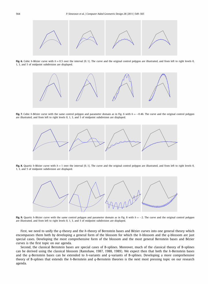
We illustrate this subdivision algorithm for h-Bézier curves in Figs. 6–9.

7. Conclusions and future work

The main focus of this paper is on developing algorithms and identities for h-Bernstein bases and h-Bézier curves usinga powerful new tool, the h-blossom. We derived an h-variant of Marsden’s identity as well as several novel change of basisformulas using h-blossoming. We also constructed new recursive evaluation algorithms for h-Bézier curves which we usedto build a recursive subdivision procedure for h-Bézier curves. In Simeonov et al. (2010) we develop similar results forq-Bernstein bases and q-Bézier curves, using another powerful variant of the classical blossom, the q-blossom.

There are many new research directions we could pursue using these new variants of blossoming. Here we mention justthe two most pressing issues.


Fig. 6. Cubic h-Bézier curve with h = 0.5 over the interval [0,1]. The curve and the original control polygon are illustrated, and from left to right levels 0,1, 3, and 5 of midpoint subdivision are displayed.

Fig. 7. Cubic h-Bézier curve with the same control polygon and parameter domain as in Fig. 6 with h = −0.46. The curve and the original control polygonare illustrated, and from left to right levels 0, 1, 3, and 5 of midpoint subdivision are displayed.

Fig. 8. Quartic h-Bézier curve with h = 1 over the interval [0,1]. The curve and the original control polygon are illustrated, and from left to right levels 0,1, 3, and 5 of midpoint subdivision are displayed.

Fig. 9. Quartic h-Bézier curve with the same control polygon and parameter domain as in Fig. 8 with h = −2. The curve and the original control polygonare illustrated, and from left to right levels 0, 1, 3, and 5 of midpoint subdivision are displayed.

First, we need to unify the q-theory and the h-theory of Bernstein bases and Bézier curves into one general theory whichencompasses them both by developing a general form of the blossom for which the h-blossom and the q-blossom are justspecial cases. Developing the most comprehensive form of the blossom and the most general Bernstein bases and Béziercurves is the first topic on our agenda.

Second, the classical Bernstein bases are special cases of B-splines. Moreover, much of the classical theory of B-splinescan be derived using the classical blossom (Ramshaw, 1987, 1988, 1989). We expect then that both the h-Bernstein basesand the q-Bernstein bases can be extended to h-variants and q-variants of B-splines. Developing a more comprehensivetheory of B-splines that extends the h-Bernstein and q-Bernstein theories is the next most pressing topic on our researchagenda.


References

Dikshit, H., Powar, P., 1982. Discrete cubic spline interpolation. Numer. Math. 40, 71–78.Dikshit, H., Rana, S., 1987. Discrete cubic spline interpolation over a nonuniform mesh. Rocky Mountain J. Math. 17, 709–718.Goldman, R., 1985. Pólya’s urn model and computer aided geometric design. SIAM J. Alg. Disc. Meth. 6, 1–28.Goldman, R., 2003. Pyramid Algorithms: A Dynamic Programming Approach to Curves and Surfaces for Geometric Modeling, The Morgan Kaufmann Series

in Computer Graphics and Geometric Modeling. Elsevier Science.Goldman, R., Barry, P., 1991. Shape parameter deletion for Pólya curves. Numer. Algorithms 1, 121–137.Lewanowicz, S., Wozny, P., 2004. Generalized Bernstein polynomials. BIT 44, 63–78.Lyche, T., 1975. Discrete polynomial spline approximation methods. Ph.D. Thesis, Department of Mathematics, University of Texas.Lyche, T., 1976. Discrete cubic spline interpolation. BIT 16, 281–290.Mangasarian, O., Schumaker, L., 1971. Discrete splines via mathematical programming. SIAM J. of Control 9, 174–183.Mangasarian, O., Schumaker, L., 1973. Best summation formula and discrete splines. SIAM J. Numer. Analysis 10, 448–459.Neamtu, M., 1991. A Contribution to the theory and practice of multivariate splines. Ph.D. Thesis, Department of Mathematics, University of Twente.Phillips, G.M., 1997a. A de Casteljau algorithm for generalized Bernstein polynomials. BIT 37, 232–236.Phillips, G.M., 1997b. Bernstein polynomials based on the q-integers. Ann. Numer. Math. 4, 511–518.Phillips, G.M., 2010. A survey of results on the q-Bernstein polynomials. IMA J. Numer. Analysis 30, 277–288.Ramshaw, L., 1987. Blossoming: A connect-the-dots approach to splines. Digital Equipment Corp., Systems Research Center, Technical Report no. 19.Ramshaw, L., 1988. Bézier and B-splines as multiaffine maps. In: Earnshaw, R.A. (Ed.), Theoretical Foundations of Computer Graphics, CAD. In: NATO ASI

Series F, vol. 40. Springer-Verlag, New York, pp. 757–776.Ramshaw, L., 1989. Blossoms are polar forms. Comput. Aided Geom. Design 6, 323–358.Rana, S., 1988. Convergence of a class of deficient interpolatory splines. Rocky Mountain J. Math. 14, 825–831.Sablonniere, P., 1992. Discrete Bézier curves and surfaces. In: Lyche, T., Schumaker, L. (Eds.), Mathematical Methods in Computer Aided Geometric Design II.

Academic Press, pp. 497–515.Schumaker, L., 1981. Spline Functions: Basic Theory. John Wiley and Sons.Simeonov, P., Zafiris, V., Goldman, R., 2010. q-Blossoming: A new approach to algorithms and identities for q-Bernstein bases and q-Bézier curves. J. Approx.

Theory, in press, doi:10.1016/j.jat.2011.09.006.Stancu, D., 1968. Approximation of functions by a new class of linear polynomial operators. Rev. Roumaine Math. Pures Appl. 13, 1173–1194.Stancu, D., 1984. Generalized Bernstein approximating operators. In: Itinerant Seminar on Functional Equations, Approximation and Convexity. Cluj-Napoca,

1984. Univ. “Babes-Bolyai”, Cluj-Napoca, pp. 185–192. Preprint 84-6.

http://dx.doi.org/10.1016/j.jat.2011.09.006

h-Blossoming: A new approach to algorithms and identities for h-Bernstein bases and h-Bézier curves

Documents

Transcript of h-Blossoming: A new approach to algorithms and identities for h-Bernstein bases and h-Bézier curves