Wireless Pers CommunDOI 10.1007/s11277-009-9865-2

GUIDE-gradient: A Guiding Algorithm for Mobile Nodesin WLAN and Ad-hoc Networks

Marco A. Gonzalez · Javier Gomez ·Miguel Lopez-Guerrero · Victor Rangel ·Martha M. Montes de Oca

© Springer Science+Business Media, LLC. 2009

Abstract Whereas there is a lot of work related to finding the location of users in WLANand ad-hoc networks, guiding users in these networks remains mostly an unexplored areaof research. In this paper we present the concept of node-to-node guidance and introduce amethod that can be used to implement it. This method relies on the computation of a localgradient in the neighborhood of the moving node. We named this protocol GUIDE-gradi-ent, which is a GPS-free and infrastructure-free node-to-node guiding system. In this paperwe also discuss how the guiding algorithm can be generalized to node-to-node guidance inmultihop ad-hoc networks.

Keywords Ad-hoc · Gradient · Guidance · RSSI · Signal quality ·WLAN

1 Introduction

The WLAN IEEE 802.11 (WiFi) standard is one of the great technology success stories of thepast decade. Used in research labs a decade ago, WiFi technology is now in a position whereit has become as popular as cellular telephony. WiFi has even become the preferred last-mile

M. A. Gonzalez (B) · J. Gomez · V. Rangel ·M. M. M. de OcaDepartment of Telecommunications Engineering,National Autonomous University of Mexico, Mexico City, Mexicoe-mail: magsunam@gmail.com

J. Gomeze-mail: javierg@fi-b.unam.mx

V. Rangele-mail: victor@fi-b.unam.mx

M. M. M. de Ocae-mail: montesdeocacaliz@gmail.com

M. Lopez-GuerreroDepartment of Electrical Engineering, Metropolitan Autonomous University,UAM-Iztapalapa, Mexico City, Mexicoe-mail: milo@xanum.uam.mx

123

M. A. Gonzalez et al.

technology of the Internet. Off-the-shelf laptops, PDAs and high-end cellular phones are nowusually equipped with WiFi radios. At the same time, metropolitan coverage with WLANnetworks is beginning to be deployed, letting WiFi users to roam freely across large areas.

In this paper we consider that the wide availability of WiFi devices enables other possibleapplications beyond data transmission. We introduce the concept of node-to-node guidancefor WiFi equipped devices. Guidance would allow WiFi equipped nodes or users to obtainguiding directions in order to get closer to other WiFi equipped devices. As it will be describedbelow, this concept can be applied to both, WLAN and ad-hoc scenarios.

Guidance, in general, and node-to-node guidance, in particular, remain mostly unexploredareas of research in WLAN and ad hoc networks. Nevertheless, we believe that there are sev-eral potentially useful node-to-node guiding applications not available to WiFi users today.For instance, we can consider a user that is currently connected to an access point (AP) at2 Mbps. Such a user can use a guiding system in order to move closer to the AP and achievea connection at a higher data rate. In another example, a user printing a document over theair to a WLAN-equipped printer can use a guiding system to get closer to the printer to pickup the print out. Rescue personnel can use a guiding system in order to get closer to a personneeding assistance, if that person is carrying a WiFi device. Applications may be as simpleas a situation where a WiFi user may just want to get closer to another user.

While in many of these situations the human eye could provide better and simpler guidingmeans, there are various scenarios where there is a need for an automatic guiding system.For instance, the presence of some obstacles may not allow a user to establish visual contactwith another user. In case the target node is not a human but a machine (e.g., APs, robots andprinters), the use of an automatic guiding system becomes mandatory. A guiding scenariothat requires special attention is the one corresponding to a situation when users are locatedfar away from each other. In this case a large distance may not allow visual contact evenwhen no obstacles are present.

We believe that one reason why there has not been much attention from the researchcommunity toward developing guiding systems for WLAN and ad-hoc networks is becausedeveloping such systems, from a pure research perspective, appears trivial once a good local-ization method is available. We argue, however, that most localization systems availabletoday are based on specialized or dedicated infrastructure (e.g., GPS or various APs). Thisdependency has, in fact, significantly reduced their availability to the larger public since notall mobile devices are currently equipped with global positioning systems, or there mightnot be enough APs in the area. Furthermore, as it will be detailed below, not all localizationsystems reported in the literature are suitable to be used as the core of a guiding system.

Before getting into the details of the proposed guiding methods, we now list what webelieve should be the desired characteristics of a guiding system in order to make it availableto the larger public for both, WLAN and ad hoc networks.

– It should operate with off-the-shelf hardware. In order to avoid extra costs we need asystem that does not need extra hardware. In contrast, WiFi is already incorporated in alllaptops, most PDAs and many high-end cellular phones.

– It should work everywhere in a distributed fashion. The use of a centralized system cannotbe considered because this would limit its availability, fault tolerance and scalability.

– It should minimize the effort needed to reach the target node. By this we mean that thespent time and traveled distance, while closing the distance to the target node, should bethe minimum. Ideally, we would like the system to guide users on a rectilinear trajectorypointing directly to the target node.

123

GUIDE-gradient: A Guiding Algorithm for Mobile Nodes

– It should work with as few as two nodes. We want the guiding system to work even if themoving and target nodes are the only nodes in the network.

– It should require a minimum intervention of the target node. It is desirable that the targetnode/user remains as passive as possible during the guiding process. Also, there shouldnot be a need to run any extra piece of software in the target node.

GUIDE is a GPS-free and infrastructure-free node-to-node guiding system for WLANand ad-hoc networks that is built around the desired characteristics described before. Oppo-site to other potential guiding systems that could be built on top of a localization system,in GUIDE wireless nodes may not know or need to know their absolute location. GUIDEis based on real-time measurements of parameters related to the state of the wireless link.Such readings come from a standard wireless card and are used in order to provide users withreal-time instructions about the required changes in direction that need to be applied in orderto get closer to the target node. Although various algorithms can be used to obtain guidingdirections from link-state measurements, in this paper we focus on a gradient-based methodthat consistently provided good results. We call this approach GUIDE-gradient.

The rest of the paper is organized as follows. Section 2 presents an overview of differentlocalization systems that could be used in the development of guiding systems. In Sect. 3we describe the different parameters that can be obtained from a standard wireless card andwe also discuss how they can be used in guiding systems. In Sect. 4 we describe GUIDE-gradient and in Sect. 5 we describe its implementation in a Linux box. In Sect. 6 we describethe experiments that were conducted and the obtained results. In Sect. 7 we describe somepractical considerations. In Sect. 8 we describe how this work can be generalized to themultihop ad hoc network case. Finally, in Sect. 9, we present our conclusions and ideas forfuture research.

2 Related Work

Beyond GPS-based guidance, which is discussed later in this section, there are not manyexamples of guiding systems for WLAN and ad-hoc networks in the literature. However,there are various localization systems that could be used as the core of a guiding system. Wenow review some of these systems.

Angle of Arrival (AoA) is a technique in which a special receiver can measure the angleon which the signal is picked up from a specific transmitter. These measurements typicallytake place at the base station where arrays of directional antennas can determine the angle ofarrival [1].

Time of arrival (ToA) [2] and Time Difference of Arrival (TDoA) [3] estimate distances bymeasuring the propagation time of a radio wave traveling from the transmitter to the receiver.ToA and TDoA techniques need tight clock synchronization for accurate distance estima-tion. The fact that propagation times in WLAN are in the order of hundreds of nanosecondsmakes it hard to accurately estimate distances using off-the-shelf WLAN hardware (e.g., aone-microsecond discrepancy represents an error of about 300 m).

Localization systems based on distance estimation are based on measurements of receivedsignal strength (RSSI) [4,5]. RSSI measurements are used, in combination with knowledgeabout transmitted power and a propagation model to estimate the distance between a trans-mitter and a receiver. Similar to ToA and TDoA techniques, measurements of signal strengthfrom various receivers and triangulation techniques can be used to reduce the uncertainty ofthe node’s location. Generally, the accuracy of these techniques is as good as the propagation

123

M. A. Gonzalez et al.

model being used. A drawback of distance-based systems is that the transmitted signal isaffected by several factors which are difficult to incorporate in a propagation model. Suchfactors can be, for instance, diverse obstructions, moving objects, the height and orientationof the antennas, etc. For this reason some proposals for localization systems that are basedon received signal strength are based on experimental propagation maps that are obtainedbeforehand.

The global positioning system (GPS) [6] may appear as the most appealing candidate toimplement guiding systems. The GPS system is based on TDoA techniques using varioussatellites in order to estimate the location of a GPS ground device. Although GPS may beused to implement a highly accurate localization system, it has several drawbacks. First,we need both, the target and moving nodes be equipped with GPS hardware plus a radiolink to communicate their coordinates to each other (i.e., cellular or WLAN radios). Thisfact alone disqualifies GPS for our purposes. Second, GPS receivers substantially increasepower consumption in a mobile device. Although it varies according to the manufacturer, aGPS device may continuously drain 50–200 mW from the battery. Finally, GPS remains anadd-on device that needs to be bought separately, thus reducing deployment possibilities andincreasing costs.

One work worth mentioning is the one recently presented in [7]. In this proposal a mobilenode combines both, GPS location data as well as RSSI information in order to estimate thelocation of an access point. The position estimation is similar to GUIDE-gradient, but itsobjective and methods are quite different to the system herein described. Furthermore, theuse of a GPS device puts this work in a different category compared to GUIDE, which is aGPS-free system.

We observe that guiding solutions based on GPS are not a practical alternative in the con-text of the node-to-node guiding system that we envision because of various factors. Othertechniques based on AoA or experimental propagation maps could provide good and cheaplocalization, but they require either special hardware or dedicated infrastructure to workproperly. Similarly, ToA and TDoA techniques cannot be considered for guiding purposesgiven the time scale of propagation times in WLAN networks. We conclude that in order tomake a guiding system available to the larger public, it is necessary to use off-the-shelf WiFiradios which are already available in many commonly used mobile devices.

3 Standard 802.11 PHY Layer Information

3.1 Channel Status Information

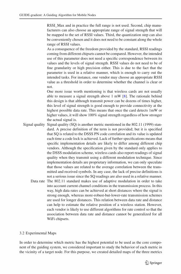
In this section we describe different parameters related to the status of the wireless channeland discuss their potential use in the implementation of a node-to-node guiding system. Sincewe are only interested in using standard WiFi hardware, we review the parameters whosemeasurements can be obtained from a standard 802.11 wireless card.

Signal strength. The energy level observed during the last protocol data unit (PDU) recep-tion is reported by means of a parameter known as received signal strengthindicator (RSSI). In the 802.11 standard the only restriction on the RSSIvalues is that there must be a minimum number of levels ranging from 0to RSSI_Max. This laxity has a number of implications. First, althoughRSSI is usually a one-byte long parameter (i.e., its value could be some-where between 0 and 255), chip vendors can choose a convenient value for

123

GUIDE-gradient: A Guiding Algorithm for Mobile Nodes

RSSI_Max and in practice the full range is not used. Second, chip manu-facturers can also choose an appropriate range of signal strength that willbe mapped to the set of RSSI values. Third, the quantization step can alsobe conveniently chosen and it does not need to be constant along the wholerange of RSSI values.As a consequence of the freedom provided by the standard, RSSI readingscoming from different chipsets cannot be compared. However, the intendeduse of this parameter does not need a specific correspondence between itsvalues and the levels of signal strength. RSSI values do not need to be offine granularity or high precision either. This is due to the fact that theparameter is used in a relative manner, which is enough to carry out theintended tasks. For instance, one vendor may choose an appropriate RSSIvalue as a threshold in order to determine whether the channel is clear ornot.One more issue worth mentioning is that wireless cards are not usuallyable to measure a signal strength above 1 mW [8]. The rationale behindthis design is that although transmit power can be dozens of times higher,this level of signal strength is good enough to provide connectivity at thehighest possible data rate. This means that once the card detects 1mW orhigher values, it will show 100% signal strength regardless of how strongerthe actual signal is.

Signal quality Signal quality (SQ) is another metric mentioned in the 802.11 (1999) stan-dard. A precise definition of the term is not provided; but it is specifiedthat SQ is related to the DSSS PN code correlation and its value is updatedeach time a code lock is achieved. Lack of further specifications means thatspecific implementation details are likely to differ among different chipvendors. Although the specification given by the standard only applies tothe DSSS modulation scheme, wireless cards also report readings of signalquality when they transmit using a different modulation technique. Sinceimplementation details are proprietary information, we can only speculatethat those values are related to the average correlation between the trans-mitted and received symbols. In any case, the lack of precise definitions isnot a serious issue since the SQ readings are also used in a relative manner.

Data rate The 802.11 standard makes use of adaptive modulation in order to takeinto account current channel conditions in the transmission process. In thisway, high data rates can be achieved at short distances where the signal isstrong enough, whereas more-robust-but-lower-rate transmission schemesare used for longer distances. This relation between data rate and distancecan help to estimate the relative position of a wireless station. However,each vendor is likely to use different algorithms for rate control so that theassociation between data rate and distance cannot be generalized for allWiFi chipsets.

3.2 Experimental Maps

In order to determine which metric has the highest potential to be used as the core compo-nent of the guiding system, we considered important to study the behavior of each metric inthe vicinity of a target node. For this purpose, we created detailed maps of the three metrics

123

M. A. Gonzalez et al.

50 m50 m

50 m

50 m

100 m

100 m

100 m

100 m

targetnode

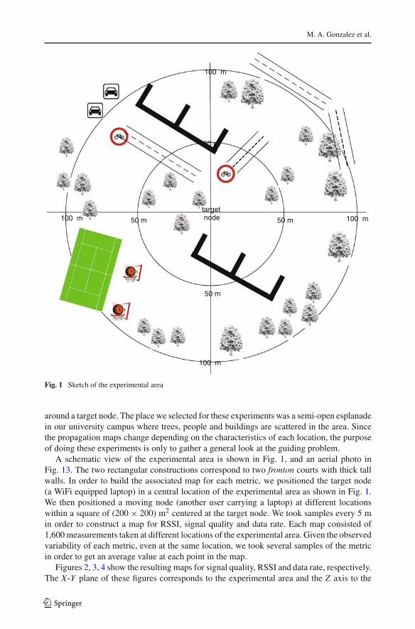
Fig. 1 Sketch of the experimental area

around a target node. The place we selected for these experiments was a semi-open esplanadein our university campus where trees, people and buildings are scattered in the area. Sincethe propagation maps change depending on the characteristics of each location, the purposeof doing these experiments is only to gather a general look at the guiding problem.

A schematic view of the experimental area is shown in Fig. 1, and an aerial photo inFig. 13. The two rectangular constructions correspond to two fronton courts with thick tallwalls. In order to build the associated map for each metric, we positioned the target node(a WiFi equipped laptop) in a central location of the experimental area as shown in Fig. 1.We then positioned a moving node (another user carrying a laptop) at different locationswithin a square of (200 × 200) m2 centered at the target node. We took samples every 5 min order to construct a map for RSSI, signal quality and data rate. Each map consisted of1,600 measurements taken at different locations of the experimental area. Given the observedvariability of each metric, even at the same location, we took several samples of the metricin order to get an average value at each point in the map.

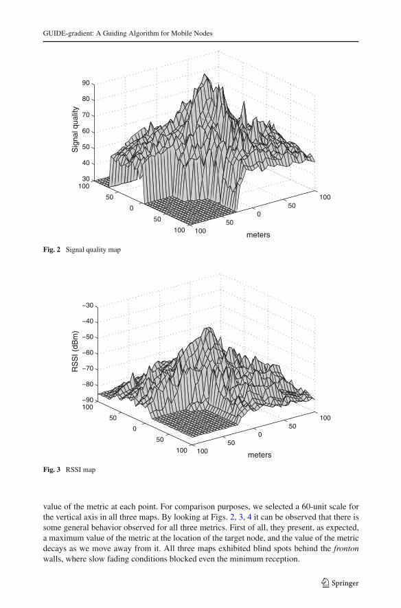
Figures 2, 3, 4 show the resulting maps for signal quality, RSSI and data rate, respectively.The X-Y plane of these figures corresponds to the experimental area and the Z axis to the

123

GUIDE-gradient: A Guiding Algorithm for Mobile Nodes

10050

050

100

100

50

0

50

10030

40

50

60

70

80

90

meters

Sig

nal q

ualit

y

Fig. 2 Signal quality map

10050

050

100

100

50

0

50

100−90

−80

−70

−60

−50

−40

−30

meters

RS

SI (

dBm

)

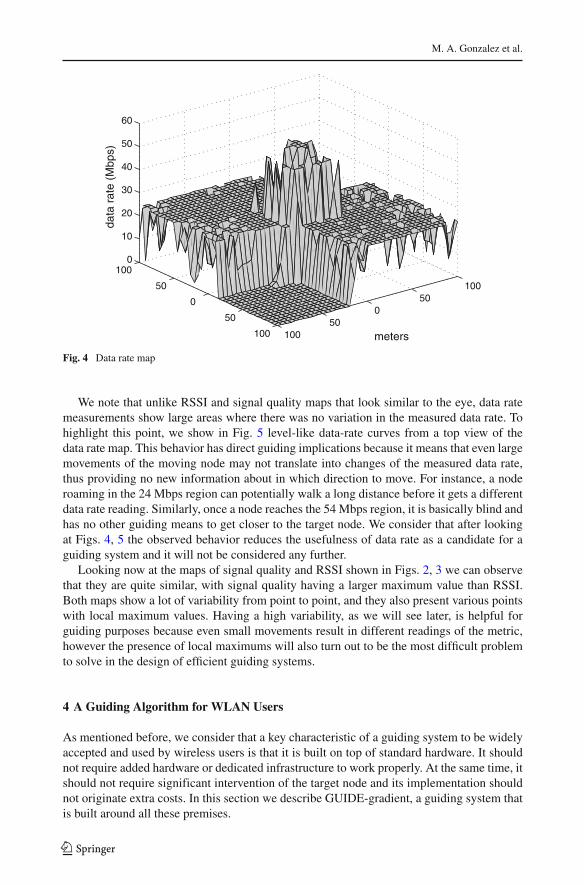
Fig. 3 RSSI map

value of the metric at each point. For comparison purposes, we selected a 60-unit scale forthe vertical axis in all three maps. By looking at Figs. 2, 3, 4 it can be observed that there issome general behavior observed for all three metrics. First of all, they present, as expected,a maximum value of the metric at the location of the target node, and the value of the metricdecays as we move away from it. All three maps exhibited blind spots behind the frontonwalls, where slow fading conditions blocked even the minimum reception.

123

M. A. Gonzalez et al.

10050

050

100

100

50

0

50

1000

10

20

30

40

50

60

meters

data

rat

e (M

bps)

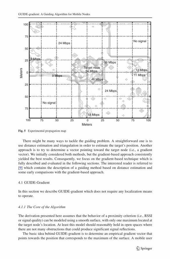
Fig. 4 Data rate map

We note that unlike RSSI and signal quality maps that look similar to the eye, data ratemeasurements show large areas where there was no variation in the measured data rate. Tohighlight this point, we show in Fig. 5 level-like data-rate curves from a top view of thedata rate map. This behavior has direct guiding implications because it means that even largemovements of the moving node may not translate into changes of the measured data rate,thus providing no new information about in which direction to move. For instance, a noderoaming in the 24 Mbps region can potentially walk a long distance before it gets a differentdata rate reading. Similarly, once a node reaches the 54 Mbps region, it is basically blind andhas no other guiding means to get closer to the target node. We consider that after lookingat Figs. 4, 5 the observed behavior reduces the usefulness of data rate as a candidate for aguiding system and it will not be considered any further.

Looking now at the maps of signal quality and RSSI shown in Figs. 2, 3 we can observethat they are quite similar, with signal quality having a larger maximum value than RSSI.Both maps show a lot of variability from point to point, and they also present various pointswith local maximum values. Having a high variability, as we will see later, is helpful forguiding purposes because even small movements result in different readings of the metric,however the presence of local maximums will also turn out to be the most difficult problemto solve in the design of efficient guiding systems.

4 A Guiding Algorithm for WLAN Users

As mentioned before, we consider that a key characteristic of a guiding system to be widelyaccepted and used by wireless users is that it is built on top of standard hardware. It shouldnot require added hardware or dedicated infrastructure to work properly. At the same time, itshould not require significant intervention of the target node and its implementation shouldnot originate extra costs. In this section we describe GUIDE-gradient, a guiding system thatis built around all these premises.

123

GUIDE-gradient: A Guiding Algorithm for Mobile Nodes

75 50 25 0 25 50 75 100

75

50

25

0

25

50

75

100

100

Target node54 Mbps

48 Mbps

12 Mbps

11 Mbps

24 Mbps

24 Mbps

18 Mbps

2 Mbps

9 Mbps

36 Mbps

No signal

No signal

Met

ers

Meters

Fig. 5 Experimental propagation map

There might be many ways to tackle the guiding problem. A straightforward one is touse distance estimation and triangulation in order to estimate the target’s position. Anotherapproach is to try to determine a vector pointing toward the target node (i.e., a gradientvector). We initially considered both methods, but the gradient-based approach consistentlyyielded the best results. Consequently, we focus on the gradient-based technique which isfully described and evaluated in the following sections. The interested reader is referred to[9] which contains the description of a guiding method based on distance estimation andsome early comparisons with the gradient-based approach.

4.1 GUIDE-Gradient

In this section we describe GUIDE-gradient which does not require any localization meansto operate.

4.1.1 The Core of the Algorithm

The derivation presented here assumes that the behavior of a proximity criterion (i.e., RSSIor signal quality) can be modeled using a smooth surface, with only one maximum located atthe target node’s location. At least this model should reasonably hold in open spaces wherethere are not many obstructions that could produce significant signal reflections.

The basic idea behind GUIDE-gradient is to determine an empirical gradient vector thatpoints towards the position that corresponds to the maximum of the surface. A mobile user

123

M. A. Gonzalez et al.

A(x,y)

C(x,y)

B(x,y)x

y

Z MA A=

Z MC C=Z MB B=

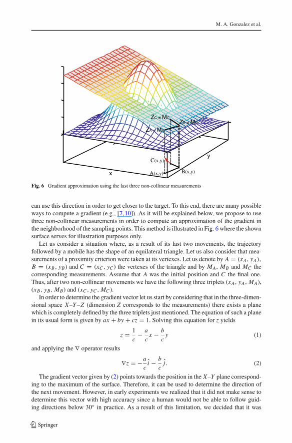
Fig. 6 Gradient approximation using the last three non-collinear measurements

can use this direction in order to get closer to the target. To this end, there are many possibleways to compute a gradient (e.g., [7,10]). As it will be explained below, we propose to usethree non-collinear measurements in order to compute an approximation of the gradient inthe neighborhood of the sampling points. This method is illustrated in Fig. 6 where the shownsurface serves for illustration purposes only.

Let us consider a situation where, as a result of its last two movements, the trajectoryfollowed by a mobile has the shape of an equilateral triangle. Let us also consider that mea-surements of a proximity criterion were taken at its vertexes. Let us denote by A = (xA, yA),

B = (xB , yB) and C = (xC , yC ) the vertexes of the triangle and by MA, MB and MC thecorresponding measurements. Assume that A was the initial position and C the final one.Thus, after two non-collinear movements we have the following three triplets (xA, yA, MA),(xB , yB , MB ) and (xC , yC , MC ).

In order to determine the gradient vector let us start by considering that in the three-dimen-sional space X–Y –Z (dimension Z corresponds to the measurements) there exists a planewhich is completely defined by the three triplets just mentioned. The equation of such a planein its usual form is given by ax + by + cz = 1. Solving this equation for z yields

z = 1

c− a

cx − b

cy (1)

and applying the ∇ operator results

∇z = −a

ci − b

cj . (2)

The gradient vector given by (2) points towards the position in the X–Y plane correspond-ing to the maximum of the surface. Therefore, it can be used to determine the direction ofthe next movement. However, in early experiments we realized that it did not make sense todetermine this vector with high accuracy since a human would not be able to follow guid-ing directions below 30◦ in practice. As a result of this limitation, we decided that it was

123

GUIDE-gradient: A Guiding Algorithm for Mobile Nodes

not necessary to compute the gradient with such a fine granularity, and we performed thequantization procedure described below.

Let us denote by−→AB,−→BC and

−→AC the displacement vectors considering the movements

from A to B, B to C and A to C , respectively. Let us consider the dot product between thegradient and each one of these displacement vectors, but let us take into consideration onlywhether the result was positive or negative. As an example, let us review which conditionssatisfy the following inequalities,

∇z · −→AB < 0, (3)

∇z · −→BC > 0 and (4)

∇z · −→AC < 0. (5)

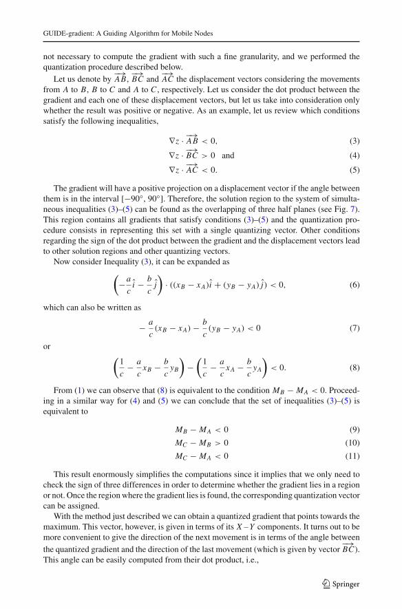
The gradient will have a positive projection on a displacement vector if the angle betweenthem is in the interval [−90◦, 90◦]. Therefore, the solution region to the system of simulta-neous inequalities (3)–(5) can be found as the overlapping of three half planes (see Fig. 7).This region contains all gradients that satisfy conditions (3)–(5) and the quantization pro-cedure consists in representing this set with a single quantizing vector. Other conditionsregarding the sign of the dot product between the gradient and the displacement vectors leadto other solution regions and other quantizing vectors.

Now consider Inequality (3), it can be expanded as(−a

ci − b

cj

)· ((xB − xA)i + (yB − yA) j) < 0, (6)

which can also be written as

− a

c(xB − xA)− b

c(yB − yA) < 0 (7)

or (1

c− a

cxB − b

cyB

)−

(1

c− a

cxA − b

cyA

)< 0. (8)

From (1) we can observe that (8) is equivalent to the condition MB − MA < 0. Proceed-ing in a similar way for (4) and (5) we can conclude that the set of inequalities (3)–(5) isequivalent to

MB − MA < 0 (9)

MC − MB > 0 (10)

MC − MA < 0 (11)

This result enormously simplifies the computations since it implies that we only need tocheck the sign of three differences in order to determine whether the gradient lies in a regionor not. Once the region where the gradient lies is found, the corresponding quantization vectorcan be assigned.

With the method just described we can obtain a quantized gradient that points towards themaximum. This vector, however, is given in terms of its X – Y components. It turns out to bemore convenient to give the direction of the next movement is in terms of the angle between

the quantized gradient and the direction of the last movement (which is given by vector−→BC).

This angle can be easily computed from their dot product, i.e.,

123

M. A. Gonzalez et al.

B

A

C

A

B

B C

A

C

BC

ACAB

θ

Gradient

(e)(d)

(a)

(b)

(c)

Fig. 7 a Displacement vectors, b region ∇z · −→AC < 0, c region ∇z · −→AB < 0, d region ∇z · −→BC > 0 ande the solution region and the corresponding quantizing vector

cos θ = �z · −→BC

| �z || −→BC |. (12)

4.1.2 The Guiding Algorithm

We introduce GUIDE-gradient, a guiding algorithm based on the following three basic move-ments: (a) if after a movement the proximity criterion improved, then the mobile can continueahead without trajectory changes, (b) if the criterion remained the same, then the mobile iscommanded to randomly turn 60◦ clockwise (CW) or counterclockwise (CCW) and, (c) if

123

GUIDE-gradient: A Guiding Algorithm for Mobile Nodes

60°60°

120°120°

M previous

M now

M previous

M now M now

M previous

M previousM now > M previousM now = M previousMnow <

Continue in thesame direction

Change thedirection 60°clockwise or

counterclockwise

Change thedirection 120°clockwise or

counterclockwise

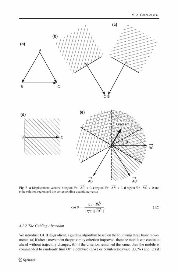
Fig. 8 Trajectory decisions in GUIDE-gradient. The variables Mnow and Mprevious stand for the current andthe previous measurements, respectively

the criterion worsened, then the mobile is commanded to turn 120◦ and move again in orderto create an equilateral triangle (in fact, as depicted in Fig. 10, two triangles can be created)and use the result described in the previous section in order to find the direction of the nextmovement. Figure 8 illustrates the three situations.

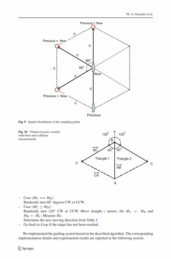
It is worth mentioning that we selected to move 60◦ when the value of the metric wasthe same in the current and previous locations, and move 120◦ when the value of the metricwas higher at the current location compared with the previous location. These decisions willcreate evenly distributed sampling points as illustrated in Fig. 9.

In what follows we describe how all these elements are put into practice in the guidingalgorithm.

GUIDE-Gradient Algorithm

Inicialization.

– Measure MA.– Move straight c meters in a randomly chosen direction. Measure MB .– Randomly turn 120◦ CW or CCW. Move straight c meters. Measure MC .– Use the turning direction selected in the previous step and {MA, MB , MC } in order to find

the the direction of the next movement by looking up the corresponding entry in Table 1.

Loop:

– Move straight c meters. Do MA ← MB and MB ← MC . Measure MC .– Compare MC and MB . The following cases are possible:– Case (MC ≥ MB)

There is no change of trajectory.

123

M. A. Gonzalez et al.

60°

60°

Previous

Now

c

c

c

c

c

c

c

Previous < Now

Previous = Now

Previous > Now

Fig. 9 Spatial distribution of the sampling points

Fig. 10 Virtual triangles createdwith three non-collinearmeasurements

Triangle 1 Triangle 2

A

B

CC

120o

120o

60 60oo

AB

BC

CA

– Case (MC == MB)

Randomly turn 60◦ degrees CW or CCW.– Case (MC ≤ MB):

Randomly turn 120◦ CW or CCW. Move straight c meters. Do MA ← MB andMB ← MC . Measure MC .Determine the new moving direction from Table 1.

– Go back to Loop if the target has not been reached.

We implemented the guiding system based on the described algorithm. The correspondingimplementation details and experimental results are reported in the following section.

123

GUIDE-gradient: A Guiding Algorithm for Mobile Nodes

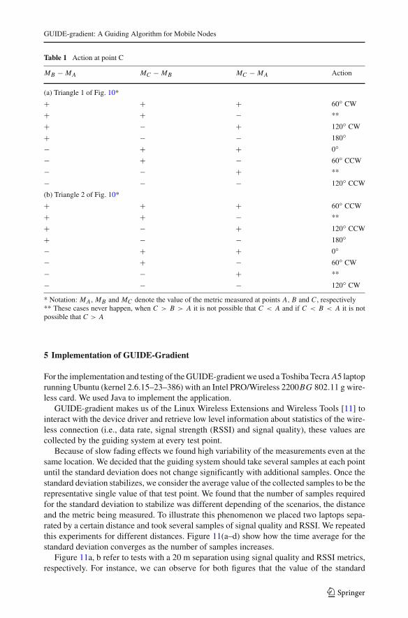
Table 1 Action at point C

MB − MA MC − MB MC − MA Action

(a) Triangle 1 of Fig. 10*

+ + + 60◦ CW

+ + − **

+ − + 120◦ CW

+ − − 180◦− + + 0◦− + − 60◦ CCW

− − + **

− − − 120◦ CCW

(b) Triangle 2 of Fig. 10*

+ + + 60◦ CCW

+ + − **

+ − + 120◦ CCW

+ − − 180◦− + + 0◦− + − 60◦ CW

− − + **

− − − 120◦ CW

* Notation: MA , MB and MC denote the value of the metric measured at points A, B and C , respectively** These cases never happen, when C > B > A it is not possible that C < A and if C < B < A it is notpossible that C > A

5 Implementation of GUIDE-Gradient

For the implementation and testing of the GUIDE-gradient we used a Toshiba Tecra A5 laptoprunning Ubuntu (kernel 2.6.15–23–386) with an Intel PRO/Wireless 2200BG 802.11 g wire-less card. We used Java to implement the application.

GUIDE-gradient makes us of the Linux Wireless Extensions and Wireless Tools [11] tointeract with the device driver and retrieve low level information about statistics of the wire-less connection (i.e., data rate, signal strength (RSSI) and signal quality), these values arecollected by the guiding system at every test point.

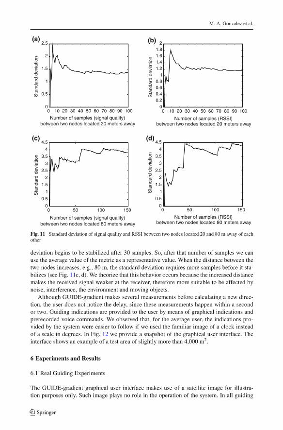
Because of slow fading effects we found high variability of the measurements even at thesame location. We decided that the guiding system should take several samples at each pointuntil the standard deviation does not change significantly with additional samples. Once thestandard deviation stabilizes, we consider the average value of the collected samples to be therepresentative single value of that test point. We found that the number of samples requiredfor the standard deviation to stabilize was different depending of the scenarios, the distanceand the metric being measured. To illustrate this phenomenon we placed two laptops sepa-rated by a certain distance and took several samples of signal quality and RSSI. We repeatedthis experiments for different distances. Figure 11(a–d) show how the time average for thestandard deviation converges as the number of samples increases.

Figure 11a, b refer to tests with a 20 m separation using signal quality and RSSI metrics,respectively. For instance, we can observe for both figures that the value of the standard

123

M. A. Gonzalez et al.

S

tand

ard

devi

atio

n

Number of samples (signal quality)between two nodes located 20 meters away

Number of samples (RSSI)between two nodes located 80 meters away

Number of samples (signal quality)between two nodes located 80 meters away

Number of samples (RSSI)between two nodes located 20 meters away

0 10 20 30 40 50 60 70 80 90 1000

0.20.40.60.8

11.21.41.61.8

2

0

0.5

1

1.5

2

2.5

0 50 100 1500

0.5

1

1.5

2

2.5

3

3.5

4

4.5(d)

(a) (b)

0 50 100 150

Sta

ndar

d de

viat

ion

0

0.5

1

1.5

2

2.5

3

3.5

4

4.5

0 10 20 30 40 50 60 70 80 90 100

Sta

ndar

d de

viat

ion

Sta

ndar

d de

viat

ion

(c)

Fig. 11 Standard deviation of signal quality and RSSI between two nodes located 20 and 80 m away of eachother

deviation begins to be stabilized after 30 samples. So, after that number of samples we canuse the average value of the metric as a representative value. When the distance between thetwo nodes increases, e.g., 80 m, the standard deviation requires more samples before it sta-bilizes (see Fig. 11c, d). We theorize that this behavior occurs because the increased distancemakes the received signal weaker at the receiver, therefore more suitable to be affected bynoise, interference, the environment and moving objects.

Although GUIDE-gradient makes several measurements before calculating a new direc-tion, the user does not notice the delay, since these measurements happen within a secondor two. Guiding indications are provided to the user by means of graphical indications andprerecorded voice commands. We observed that, for the average user, the indications pro-vided by the system were easier to follow if we used the familiar image of a clock insteadof a scale in degrees. In Fig. 12 we provide a snapshot of the graphical user interface. Theinterface shows an example of a test area of slightly more than 4,000 m2.

6 Experiments and Results

6.1 Real Guiding Experiments

The GUIDE-gradient graphical user interface makes use of a satellite image for illustra-tion purposes only. Such image plays no role in the operation of the system. In all guiding

123

GUIDE-gradient: A Guiding Algorithm for Mobile Nodes

Guiding algorithm: Distance Based (RSSI)

Moving speed:

Metric: -60

1.0

Start Reset Stop ContinueStart

Targetnode

Gradient Based (SQ)

m/s

dBm

Fig. 12 GUIDE-gradient graphical user interface

experiments the moving node was initially located at the center of the experimental areaand the target node was placed a hundred meters away in an arbitrary position. These pointsappear in the figures at positions labeled as “Start” and “Target Node” respectively. Thedistance that the moving node travels between stop points was set to 20 m.

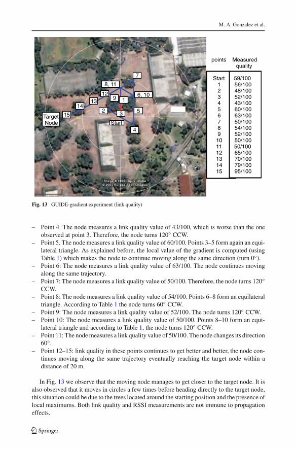
In Fig. 13 we provide an example of the full guiding path while using GUIDE-gradient.In this figure we show the full path followed by the moving node along with the value of themetric measured at each point. In this experiment the user stopped moving when he or shereached a distance of less than 20 m with respect to target node, to mark this stop-point weshow a circle around the target node with a 20-m radius. When the program starts, the usermust indicate his or her approximate walking speed so that the program can approximatelydetermine the time it takes to move the intended distance.

6.1.1 Experiments with GUIDE-Gradient

Figure 13 shows a guiding experiment using the GUIDE-gradient algorithm with signal qual-ity as the metric. It can be observed that even though there are several guiding impairments,after a few movements the guiding system was able to find the target node. For illustrativepurposes we detail the trajectory decisions taken by GUIDE-gradient.

– Start. The node measures a link quality value of 59/100 and (randomly) moves to adirection that corresponds to the top of Fig. 13.

– Point 1. The node measures a link quality value of 56/100 which is worse than theone observed at point 0. Therefore, the node turns 120◦ counterclockwise (CCW) in thiscase.

– Point 2. The node measures a link quality value of 48/100. Points 0–2 form an equilateraltriangle. According to the rules shown in Table 1, the node turns 120◦ CCW.

– Point 3. The node measures a link quality value of 52/100, which is better than the oneobserved at point 2, therefore, the node continues moving along the same trajectory.

123

M. A. Gonzalez et al.

Start

points Measuredquality

Start 59/1001 56/1002 48/1003 52/1004 43/1005 60/1006 63/1007 50/1008 54/1009 52/10010 50/10011 50/10012 65/10013 70/10014 79/10015 95/100

TargetNode

12

2 3

4

5

6, 10

7

8, 11

913

14

15

1

Fig. 13 GUIDE-gradient experiment (link quality)

– Point 4. The node measures a link quality value of 43/100, which is worse than the oneobserved at point 3. Therefore, the node turns 120◦ CCW.

– Point 5. The node measures a link quality value of 60/100. Points 3–5 form again an equi-lateral triangle. As explained before, the local value of the gradient is computed (usingTable 1) which makes the node to continue moving along the same direction (turn 0◦).

– Point 6: The node measures a link quality value of 63/100. The node continues movingalong the same trajectory.

– Point 7: The node measures a link quality value of 50/100. Therefore, the node turns 120◦CCW.

– Point 8: The node measures a link quality value of 54/100. Points 6–8 form an equilateraltriangle. According to Table 1 the node turns 60◦ CCW.

– Point 9: The node measures a link quality value of 52/100. The node turns 120◦ CCW.– Point 10: The node measures a link quality value of 50/100. Points 8–10 form an equi-

lateral triangle and according to Table 1, the node turns 120◦ CCW.– Point 11: The node measures a link quality value of 50/100. The node changes its direction

60◦.– Point 12–15: link quality in these points continues to get better and better, the node con-

tinues moving along the same trajectory eventually reaching the target node within adistance of 20 m.

In Fig. 13 we observe that the moving node manages to get closer to the target node. It isalso observed that it moves in circles a few times before heading directly to the target node,this situation could be due to the trees located around the starting position and the presence oflocal maximums. Both link quality and RSSI measurements are not immune to propagationeffects.

123

GUIDE-gradient: A Guiding Algorithm for Mobile Nodes

0 500 1000 15000

0.1

0.2

0.3

0.4

0.5

0.6

0.7

0.8

0.9

1

distance traveled (m)

%

CDF

Ideal caseGradient−RSSI−10Gradient−RSSI−20Gradient−RSSI−30Gradient−SQ−10Gradient−SQ−20Gradient−SQ−30

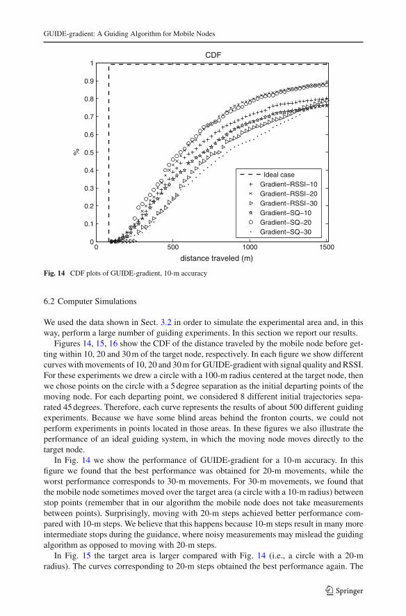
Fig. 14 CDF plots of GUIDE-gradient, 10-m accuracy

6.2 Computer Simulations

We used the data shown in Sect. 3.2 in order to simulate the experimental area and, in thisway, perform a large number of guiding experiments. In this section we report our results.

Figures 14, 15, 16 show the CDF of the distance traveled by the mobile node before get-ting within 10, 20 and 30 m of the target node, respectively. In each figure we show differentcurves with movements of 10, 20 and 30 m for GUIDE-gradient with signal quality and RSSI.For these experiments we drew a circle with a 100-m radius centered at the target node, thenwe chose points on the circle with a 5 degree separation as the initial departing points of themoving node. For each departing point, we considered 8 different initial trajectories sepa-rated 45 degrees. Therefore, each curve represents the results of about 500 different guidingexperiments. Because we have some blind areas behind the fronton courts, we could notperform experiments in points located in those areas. In these figures we also illustrate theperformance of an ideal guiding system, in which the moving node moves directly to thetarget node.

In Fig. 14 we show the performance of GUIDE-gradient for a 10-m accuracy. In thisfigure we found that the best performance was obtained for 20-m movements, while theworst performance corresponds to 30-m movements. For 30-m movements, we found thatthe mobile node sometimes moved over the target area (a circle with a 10-m radius) betweenstop points (remember that in our algorithm the mobile node does not take measurementsbetween points). Surprisingly, moving with 20-m steps achieved better performance com-pared with 10-m steps. We believe that this happens because 10-m steps result in many moreintermediate stops during the guidance, where noisy measurements may mislead the guidingalgorithm as opposed to moving with 20-m steps.

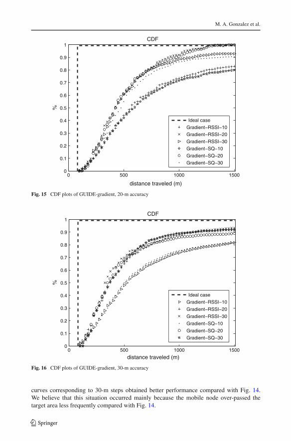
In Fig. 15 the target area is larger compared with Fig. 14 (i.e., a circle with a 20-mradius). The curves corresponding to 20-m steps obtained the best performance again. The

123

M. A. Gonzalez et al.

0 500 1000 15000

0.1

0.2

0.3

0.4

0.5

0.6

0.7

0.8

0.9

1

distance traveled (m)

%

CDF

Ideal case

Gradient−RSSI−10

Gradient−RSSI−20

Gradient−RSSI−30

Gradient−SQ−10

Gradient−SQ−20

Gradient−SQ−30

Fig. 15 CDF plots of GUIDE-gradient, 20-m accuracy

0 500 1000 15000

0.1

0.2

0.3

0.4

0.5

0.6

0.7

0.8

0.9

1

distance traveled (m)

%

CDF

Ideal case

Gradient−RSSI−10

Gradient−RSSI−20

Gradient−RSSI−30

Gradient−SQ−10

Gradient−SQ−20

Gradient−SQ−30

Fig. 16 CDF plots of GUIDE-gradient, 30-m accuracy

curves corresponding to 30-m steps obtained better performance compared with Fig. 14.We believe that this situation occurred mainly because the mobile node over-passed thetarget area less frequently compared with Fig. 14.

123

GUIDE-gradient: A Guiding Algorithm for Mobile Nodes

In Fig. 16 we increased the target area to a circle with a 30-m radius. In this figure thecurves with steps of 20 and 30 m obtained the best performance, while the curves with 10-msteps obtained lower performance.

Looking at Figs. 14, 15, 16 we conclude that using 10-m steps for GUIDE-gradient withsignal quality and RSSI may not be a good design choice. This happens because from pointto point, there may not be enough variability of the metric being measured. This, in turn, willcreate more triangles in the guidance where the mobile node wastes time. Similarly, perfor-mance of guiding using large steps improves as the target area becomes similar or larger insize than the step size.

7 GUIDE-Gradient Considerations

There are a number of considerations that are taken into account for a correct operation ofGUIDE-gradient in some practical situations. In particular, the following two situations areconsidered in our system.

As explained in the operation of GUIDE-gradient, mobile nodes always move along rec-tilinear trajectories according to the directions given by the system. In open areas, this maynot be a difficult task to fulfill, however, in semi-open or indoor areas, obstacles may notallow a user to move along the desired trajectory. For instance, it may happen that a mobilenode finds a wall and it is forced to move to one side. Moving along a different trajectoryfrom the one specified by the system clearly misleads the guiding system, since the locationestimated by the system and the real location of the user will be different. In such cases it isnecessary that the user has a way of telling the system which trajectory is actually using.

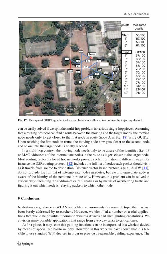
In GUIDE-gradient this is done by using the graphical user interface shown in Fig. 12.When an obstacle blocks the user’s intended trajectory, the user should come to a stop, clickon the Reset option and visually select a new clear trajectory. The Reset option has the effectof restarting the guiding process, keeping no memory of previous movements. In Fig. 17 weshow an example of this situation when after reaching point 3, a large building does not allowa user to continue moving forward as indicated by the algorithm. At that point the user stops,resets the algorithm and then starts moving along the chosen trajectory. In Fig. 17 points 1’ to3’ and points 1” to 12” correspond to two separate and independent attempts to reach thetarget node.

The second situation is related to what happens if during the guiding process a mobileuser losses its link to the target node by moving out of range. This situation will be a commoncase when the mobile user is located at the edge of the target node’s range. In this case wetook a simple solution where the mobile user returns to its previous point in case it losses thelink with the target node.

8 On Node-to-node Guidance in Ad hoc Networks

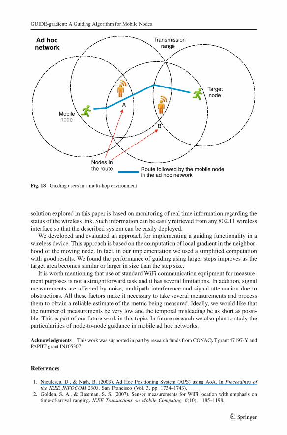
In this section we comment on how the guiding system can be generalized to multi-hop ad hoc systems. Similar to WLAN technology, so far there has not been significantresearch related to guiding users in ad hoc networks. In ad hoc networks there may be sev-eral intermediate nodes, working as relays in the communication path between the movingand the target node. Figure 18 illustrates an example of a multi-hop route involving twointermediate nodes. While the guiding problem in multi-hop ad hoc networks may appear farmore complex than the simpler WLAN (single-hop) problem that we have been addressing, it

123

M. A. Gonzalez et al.

Targetnode

Start

1'

2'

4''

3''

2''

1''

3'

5''

9''

7''

8''

6'' 10''

11''

12''

points Measuredquality

Start 55/1001' 57/1002' 59/1003' 61/100

60/1001'' 57/1002'' 63/1003'' 67/1004'' 65/1005'' 70/1006'' 70/1007'' 68/1008'' 72/1009'' 77/10010'' 84/10011'' 82/10012'' 91/100

ResetReset

Fig. 17 Example of GUIDE-gradient where an obstacle not allowed to continue the trajectory desired

can be easily solved if we split the multi-hop problem in various single-hop pieces. Assumingthat a routing protocol can find a route between the moving and the target nodes, the movingnode needs only to get closer to the first node in route (node A in Fig. 18) using GUIDE.Upon reaching the first node in route, the moving node now gets closer to the second nodeand so on until the target node is finally reached.

In a multi-hop context, the moving node needs only to be aware of the identities (i.e., IPor MAC addresses) of the intermediate nodes in the route as it gets closer to the target node.Most routing protocols for ad hoc networks provide such information in different ways. Forinstance the DSR routing protocol [12] includes the full list of nodes each packet should visitas it travels from source to destination. Distance vector based protocols (e.g., AODV [13])do not provide the full list of intermediate nodes in routes, but each intermediate node isaware of the identity of the next one in route only. However, this problem can be solved invarious ways including the addition of extra signaling or by means of overhearing traffic andfiguring it out which node is relaying packets to which other node.

9 Conclusions

Node-to-node guidance in WLAN and ad-hoc environments is a research topic that has justbeen barely addressed by researchers. However, we identified a number of useful applica-tions that would be possible if common wireless devices had such guiding capabilities. Weenvision many possible applications that range from everyday tasks to critical ones.

At first glance it may seem that guiding functions can be incorporated in a wireless deviceby means of specialized hardware only. However, in this work we have shown that it is fea-sible to use standard WiFi devices in order to provide a reasonable guiding experience. The

123

GUIDE-gradient: A Guiding Algorithm for Mobile Nodes

Transmissionrange

Mobilenode

Nodes inthe route

A

B

Route followed by the mobile nodein the ad hoc network

Targetnode

Ad hocnetwork

Fig. 18 Guiding users in a multi-hop environment

solution explored in this paper is based on monitoring of real time information regarding thestatus of the wireless link. Such information can be easily retrieved from any 802.11 wirelessinterface so that the described system can be easily deployed.

We developed and evaluated an approach for implementing a guiding functionality in awireless device. This approach is based on the computation of local gradient in the neighbor-hood of the moving node. In fact, in our implementation we used a simplified computationwith good results. We found the performance of guiding using larger steps improves as thetarget area becomes similar or larger in size than the step size.

It is worth mentioning that use of standard WiFi communication equipment for measure-ment purposes is not a straightforward task and it has several limitations. In addition, signalmeasurements are affected by noise, multipath interference and signal attenuation due toobstructions. All these factors make it necessary to take several measurements and processthem to obtain a reliable estimate of the metric being measured. Ideally, we would like thatthe number of measurements be very low and the temporal misleading be as short as possi-ble. This is part of our future work in this topic. In future research we also plan to study theparticularities of node-to-node guidance in mobile ad hoc networks.

Acknowledgments This work was supported in part by research funds from CONACyT grant 47197-Y andPAPIIT grant IN105307.

References

1. Niculescu, D., & Nath, B. (2003). Ad Hoc Positioning System (APS) using AoA. In Proceedings ofthe IEEE INFOCOM 2003, San Francisco (Vol. 3, pp. 1734–1743).

2. Golden, S. A., & Bateman, S. S. (2007). Sensor measurements for WiFi location with emphasis ontime-of-arrival ranging. IEEE Transactions on Mobile Computing, 6(10), 1185–1198.

123

M. A. Gonzalez et al.

3. Yamasaki, R., Ogino, A., Tamaki, T., Uta, T., Matsuzawa, N., & Kato, T. (2005). TDOA location systemfor IEEE 802.11b WLAN. In Proceedings of the IEEE Wireless Communications and NetworkingConference (WCNC05) (Vol. 4, pp. 2338–2343).

4. Bahl, P., & Padmanabhan, V. N. (2002). Radar: An in-building RF-based user location and trackingsystem. In Proceedings of IEEE INFOCOM 2002 (pp. 7–9). Tel Aviv, Israel.

5. Kitasuka, T., Hisazumi, K., Nakanishi, T., & Fukuda, A. (2005). Positioning techniques of wirelessLAN terminals using RSSI between terminals. In Proceedings of the 2005 International Conferenceon Pervasive Systems and Computing (PSC-05) (pp. 47–53). Las Vegas, Nevada, USA.

6. Parkinson, B. W., & Spilker, J. J. Jr. (1996). Global positioning system: Theory and application.American Institute of Astronautics and Aeronautics.

7. Han, D., Andersen, D. G., Kaminsky, M., Papagiannaki, K., & Seshan, S. (2009). Access point local-ization using local signal strength gradient. In S. Moon & R. Teixeira (Eds.), Network measurement,LNCS 5448 (pp. 91–100). Berlin, Heidelberg: Springer.

8. Bardwell, J. (2004). You believe you understand what you think I said...—the truth about 802.11signal and noise metrics. Connect 802 Corporation, white paper.

9. Gonzalez, M., Gomez, J., Lopez-Guerrero, M., Rangel, V., & Torres-Fernandez, J. E. (2008). GUIDE:Guiding users in distributed environments for WLAN and Ad hoc networks. In Networking andElectronic Commerce Research Conference 2008, ISBN: 978-0-9820958-0-5. Riva del Garda, Italia.

10. Henderson, T. C., & Grant, E. (2004). Gradient calculation in sensor networks. In Proceedings of2004 IEEERSI lnternatlonal Conference on Intelligent Robots and Systems (pp. 1792–1793). Sendai,Japan.

11. Tourrilhes, J. (2008). Wireless tools for Linux, Hewlett Packard, date of last update:January 16, 2008,date of consultation:July 14, 2008, from http://hpl.hp.com/personal/Jean-Tourrilhes/Linux/Tools.html.

12. Johnson, D. B., Maltz, D. A., & Broch, J. (2001). DSR: The dynamic source routing protocol formulti-hop wireless ad hoc networks. In C. E. Perkins (Ed.), Ad Hoc networking (Chap. 5, pp. 139–172).Boston, MA: Addison-Wesley.

13. Perkins, C. E., & Royer, E. M. (1999). Ad hoc on-demand distance vector routing. Proceedings ofthe 2nd IEEE Workshop on Mobile Computing Systems and Applications (pp. 90–100). New Orleans,LA.

Author Biographies

Marco A. Gonzalez received the B.Sc. in Computer Engineering andthe M.Sc. in Computer Engineering from the National AutonomousUniversity of Mexico (UNAM). He has worked as project coordina-tor in the design and implementation of cross connection solutionsfor LAN, ISDN, Frame Relay, ATM and xDSL technologies. He iscurrently a Ph.D. student at UNAM.

Javier Gomez received the B.Sc. degree with honors in ElectricalEngineering in 1993 from the National Autonomous University ofMexico (UNAM) and the M.S. and Ph.D. degrees in Electrical Engi-neering in 1996 and 2002, respectively, from Columbia Universityand its COMET Group. During his Ph.D. studies at Columbia Uni-versity, he collaborated and worked on several occasions at the IBMT.J. Watson Research Center, Hawthorne, New York. His researchinterests cover routing, QoS, and MAC design for wireless ad hoc, sen-sor, and mesh networks. Since 2002, he has been an Assistant Professorwith the National Autonomous University of Mexico. Javier Gomez ismember of the SNI (level I) since 2004.

123

GUIDE-gradient: A Guiding Algorithm for Mobile Nodes

Miguel Lopez-Guerrero received his B.Sc. with honors in Mechan-ical—Electrical Engineering in 1995 and the M.Sc. with honors inElectrical Engineering in 1998, both from the National AutonomousUniversity of Mexico. He received his Ph.D. in Electrical Engineer-ing from the University of Ottawa in 2004. Currently, he is an Asso-ciate Professor with the Metropolitan Autonomous University (MexicoCity). His areas of interest are medium access control, traffic control,and traffic modeling.

Victor Rangel obtained his Bachelor Degree in Computer Engineer-ing from the National Autonomous University of Mexico (UNAM).He obtained his Master Degree in Data Communication Systems andhis doctoral degree in Telecommunications Engineering from the Cen-tre for Mobile Communications Research, The University of Sheffield(England). His Ph.D. thesis focused on the modeling and analysis ofCable TV networks supporting broadband Internet traffic. Dr. Rangel iscurrently a professor at the Department of TelecommunicationsEngineering, School of Engineering (UNAM).

Martha M. Montes de Oca received her B.Sc. with honors in Infor-matics and the M.Sc. in Computer Engineering from the NationalAutonomous University of Mexico (UNAM). She has worked as Serv-ers and Network Manager and Programmer Senior. He is currently aPh.D. student at UNAM.

123